precision measurement of neutrino oscillation parameters at

Precision measurement ofneutrino oscillation parameters

at INO ICAL

By

Lakshmi S Mohan

Enrolment Number : PHYS01200904008

Bhabha Atomic Reseaarch Centre

Mumbai - 400 085

A thesis submitted to

The Board of Studies in Physical Sciences

In partial fulfillment of requirements

For the Degree of

DOCTOR OF PHILOSOPHY

of

HOMI BHABHA NATIONAL INSTITUTE

October, 2015

Homi Bhabha National InstituteRecommendations of the Viva Voce Board

As members of the Viva Voce Board, we certify that we have read the dissertation prepared by Lak-

shmi S Mohan (PHYS01200904008) entitled “Precision measurement of neutrino oscillation parameters at

INO ICAL” and recommend that it may be accepted as fulfilling the dissertation requirement for the Degree

of Doctor of philosophy.

Date:

Chairman -

Date:

Guide / Convener -

Date:

Member 1 -

Date:

Member 2 -

Date:

Member 3 -

Date:

External Examiner -

Final approval and acceptance of this dissertation is contingent upon the candidate’s submission

of the final copies of the dissertation to HBNI.

I hereby certify that I have read this dissertation prepared under my direction and recommend

that it may be accepted as fulfilling the dissertation requirement.

Date:

Place: Guide

3

STATEMENT BY AUTHOR

This dissertation has been submitted in partial fulfillment of requirements for an advanced degree at Homi

Bhabha National Institute (HBNI) and is deposited in the Library to be made available to borrowers under

rules of the HBNI.

Brief quotations from this dissertation are allowable without special permission, provided that accu-

rate acknowledgement of source is made. Requests for permission for extended quotation from or repro-

duction of this manuscript in whole or in part may be granted by the Competent Authority of HBNI when

in his or her judgement the proposed use of the material is in the interests of scholarship. In all other

instances, however, permission must be obtained from the author.

Lakshmi S Mohan

(Enrolment Number : PHYS01200904008)

Date:

Place:

5

Declaration

I hereby declare that the investigation presented in the thesis has been carried out

by me. The work is original and has not been submitted earlier as a whole or in part for a

degree/diploma at this or any other Institution/University.

Lakshmi S Mohan


Date:

Place:

7

Dedicated to

My Parents

ACKNOWLEDGEMENTS

Dreams and aspirations

I honestly don’t know where to start this acknowledgement. I am wordless right now to

express the depth of my gratitude to all the people who have guided, supported, pushed,

pulled and cared for an ordinary girl who just wanted to do Physics all her life. And the

girl was lucky enough to have joined the most ambitious basic science projects in India

and be part of a huge academic family aka the INO collaboration. :)

Nowords will be sufficient enough to express how lucky I feel to have been guided by

Prof. D. Indumathi, IMSc, one of the most brilliant Physicists I have ever known. Without

the excellent guidance Ma’am gave and the support both academic and personal and her

loving care, I would never have reached this point. Ma’am’s wisdom and knowledge are

unparalleled and farsighted nature and prudence, something to learn from. I express,

from the bottom of my heart, my many thanks and gratitude to Indu Ma’am, for being

kind, patient and loving to an ordinary student like me and for the immense support and

motivation all throughout this PhD period. Thank you Ma’am for being my guide and

light all these years.

I thank Prof. M.V.N.Murthy, IMSc, for all the guidance given to us young students.

As the co-ordinator of the hadron group of the INO ICAL collaboration he gave us the

opportunity to work under his guidance. Again the guidance and care Prof. Murthy

gave cannot be expressed in words. The neutrino physics lectures he used to give us

on Saturdays were really memorable. I express my heartfelt gratitude and thanks to

Prof.M.V.N.Murthy for the great guidance and support he gave to a budding student.

Again words will not be enough to express my gratitude.

I thank Prof.Nita Sinha, IMSc for the care and support she has given me as a student.

I also express my heartfelt thanks to Prof. G. Rajasekharan, IMSc and CMI, for being

an inspiration to a young student like me. I was lucky enough to be part of the INO

collaboration and work in the Institute of Mathematical Sciences and interact with these

great scientists and teachers.

I thank my doctoral committee members, Prof.James Libby, IITM and Prof. Prafulla

Behera IITM, for the timely advises and comments and support. Being in a collaboration

is a great experience. INO is special in that it gave me an opportunity to go to several

institutes and work there. That also means that I had the opportunity to be taught by

11

12

many amazing scientists. In the Tata Institute of Fundamental Reseaarch (TIFR) Mumbai,

where I did my PhD course work, I was taught by some of the most amazing scientists. I

thank Prof. Naba K Mondal, INO project director for all the guidance and support he has

offered not only as the director of such a mega science project but also as an enthusiastic

teacher who used to spend time discussing detector physics with us in the first year of

PhD. Prof. Mondal’s great dedication to science is inspirational and the ease with which

he sees the whole picture of an analysis and makes the right comments can only come

with experience and passion to science. Thank you Sir for being so energetic and caring.

I express my heartfelt gratitude to Prof. Amol Dighe, who not only taught us neutrino

physics during course work, but also happened to be my collaborator’s guide and one

of the coordinators of the ICAL physics group. His classes were really enjoyable. Being

a member of the hadron group, I got the opportunity to discuss with him even though

a little. Thank you Sir, for all the kind suggestions both in the discussions and in the

physics meetings and careful readings of all the drafts.

I express my heartfelt gratitude to Prof. Gobinda Majumder, who taught us during

our course work and is the author of the ICAL simulation code which we students have

been using for all the PhD works. I thank Prof. Majumder for all the prompt help and

clarifications he has given regarding detector simulations during the PhD time. I thank

Prof.Kajari Mazumdar, Prof. Vandana Nanal, Prof. R.G.K Pillai, Prof. Sudeshna Banerjee,

TIFR, and Prof. L.M.Pant, BARC, who taught us and enlightened us on various fields

during our course work in the first year of PhD and cared for us. I express my heartfelt

thanks to Dr. Satyanarayana Bheesette, for being our mentor and for all the care and

support bestowed on students.

I express my gratitude to Prof. Md. Naimuddin, Delhi university and Prof. Prafulla

Behera, IITM, for co-ordinating all the detector simulation meetings and all the sugges-

tions and discussions regarding detector simulations. I express my heartfelt thanks to

Prof.Amol Dighe, TIFR and Prof.Srubabati Goswami, PRL, for co-ordinating the physics

simulation meetings and the wise suggestions and comments. I also thank Prof. Sandhya

Choubey, earlier coordinator of physics group along with Prof.D. Indumathi, and a mem-

ber of the hadron simulations group, for the suggestions and comments and support. I

thank Prof.Y. P. Viyogi, VECC; Prof. Vivek Datar, BARC and Prof. Brajesh Choudhary,

Delhi University for the careful reading, suggestions and comments on the hadron simu-

lation reports. I also express my thanks to Prof. Uma Shankar, IITB; Prof. Satyajit Saha,

13

SINP and Prof. Sanjib Kumar Agarwalla, IOP. I express my heartfelt thanks to Ms.Asmita

Redij, for the development of the ICAL simulation code and the clarifications she would

offer.

I express my thanks to the scientific staff in TIFR involved with the R&D of RPCs,

Mr. S. Kalmani, Mr. L. V Reddy, Mr.Ravindra R Shinde, Mr. Mandar Saraf, Mr. Manas

Bhuyan, Mr. S. Chavan,Mr. G. Ghodke andMr. P. Nagraj, Ms. N. Srivastava andMr. V. Pa-

van Kumar for all the computer related helps in TIFR. I have to express my heartfelt

gratitude towards the system administrators of the Institute of Mathematical Sciences,

Sri.G. Subramoniam and Sri. Raveendra Reddy B, for the amazing computing facilities,

enabling fast and efficient computing. I express my gratitude to Sri.Mangala Pandi,

project system administrators, IMSc for all the prompt help regarding the cluster ma-

chines in IMSc were I used to run all the simulations required for my work. I express my

heartfelt thanks to Mr. Srinivasan and Mr. Jahir Hussain, technical assistants, computer

section for all the help they have given regarding all kinds of computers and comput-

ing. Without the excellent clusters of IMSc my PhD would not have been a reality! Bravo

Satpura6!

At this point I express my gratitude to all members of the INO collaboration who have

been lending their direct and indirect support and care all throughout. INO collaboration

meetings were all memorable and it was a great experience being part of the collabora-

tion being able to interact with so many people and learn from them. I also express my

heartfelt thanks to the administrative staff of both TIFR and IMSc for taking care of all

our official matters, be it salary or accommodation or anything else and giving all the

support so that we could do our research work without bothering about anything else. I

thank the Department of Atomic Energy (DAE), India and the Department of Science and

Technology (DST), India for jointly funding this research.

I thank with great respect all the teachers who have taught me in school, college

and university. Without their guidance and support I would not have made it to the

beginning of the PhD. I express my heartfelt thanks to Prof.K. Indulekha, Prof. C. Venu-

gopal and Prof. N.V.Unnikrishnan, Mahatma Gandhi University, for the care and sup-

port given to me as a student. I humbly bow my head in the memories of Late. Prof.

G.V.Vijayagovindan M.G.University and Late. Prof. Rahul Basu, IMSc, who guided me

to high energy physics and whom I will always remember with great respect.

I expressmy special thanks tomy student collaborators MoonMoonDevi, Dr. Anushree

14

Ghosh, and Daljeet Kaur. It was pleasure working with you all. Moon Moon thank you

for being my friend apart from being a great collaborator and for being there to push,

pull, scold, support, love and care in times of need and for that nudge you would give for

making me confident enough to be independent. I express my heartfelt thanks to Kan-

ishka Rawat, for being a steadfast friend and for all the love and care she has given me

again in times of need. Again, thanks to my two great pillars of support Moon Moon and

Kanishka for being those strong friends who not only gave me the gift of friendship, but

to whom I could give the gift of friendship and care as well.

Friends are those who keep life colourful. I thank my INO student friends Meghna,

Mathimalar, Neha, Animesh, Sumanta, Vivek, Nitali, Anushree, Sudeshna, Chandan,

Amina, Raveendra, Rajesh Ganai, Varchaswi, Ali, Abhik and Deepak for being part of

this INO student family. A very special thanks to Dr.Saveetha and Senthil, IMSc, for be-

ing friends and members of the IMSc group. Also special thanks to the students in the

Chennai group Meghna, Divya, Aleena, Rebin and Saddique. Special thanks to Dr. Sus-

nata Seth, Post Doc at TIFR. I also thank Dr.Shreedevi K Masuti, Dr.Pradeesha Ashok and

Sruthi Murali who were my flat mates in IMSc. The times I spent with you as flatmates

are memorable and will be missed. Thank you deeply for the love and care you all kindly

bestowed on me. I also thank Sriluckshmy P V, my flatmate and research scholar in IMSc.

I cannot end the list of friends I want to acknowledge without mentioning Dr.Meenadevi,

Debasmita Mukherjee, Ria Sain, Jilmy, Minati, Tanmay Mitra and Dr.Jaya Maji and baby

Arama, who have been kind enough to be my friends in IMSc. I also thank Abhrajit

Laskar and Rajesh Singh, my office mates for being studious and hard working, looking

at whom I could come back on track if ever I felt like slacking off.

This comes last, nevertheless very important, for family is what keeps you firm and

extends all love and care always. I thank my family for the biggest support anybody

could ever give. Words won’t be sufficient to express how deeply I am indebted to my

parents Sri.R. Mohanachandran and Smt.N. S. Sandhyakumari. All my urge to study has

come from them only. As a kid I used to make them tell me about their younger days and

unknowingly picked up the lesson that they came up in life because of their education.

My parents took all the best efforts to give me the best possible education. I am lucky to

have been born as the daughter of such loving parents. Hopefully someday I will make

them proud. I also thank my relatives, especially my grandmother and grandaunts who

actually supported and gave courage to my parents when they were afraid of sending me

15

to a distant place for PhD. I thank all my near and distant family members for all the care

and support they have given me. Thank you all for being that great support all the time.

An eight year old girl read about the Solar System in a children’s magazine special edition.

It was so impressive to know that we live on a planet which is part of something bigger. Then in

school she learned that the solar system is part of a galaxy and the galaxy is part of the universe

and so on. The girl used to dream about roaming in the skies on the clouds or travelling the whole

universe touching stars and going inside them and travelling forever enjoying the myriad wonders

out there. I am thankful that, that girl has not changed, even though she has grown up and her

outer world and life in general have changed. Thankfully she never gave up on her dream and

somehow managed to battle obstacles and get past them, difficult they might have been. And she

still dreams that someday she will traverse those places in the visible night sky she admires and

those invisible places out there.

Thank you Nature, for being so mysteriously beautiful, holding never ending surprises.

LIST OF PUBLICATIONS

• Published in refereed journals

1. M.M. Devi, A. Ghosh, D. Kaur, S.M. Lakshmi, et al., “Hadron energy response of

the Iron Calorimeter detector at the India-based Neutrino Observatory”, JINST

8, P11003, 2013 [arXiv:1304.5115 [physics.ins-det]].

2. S.M. Lakshmi, A. Ghosh, M.M. Devi, D. Kaur, et al., “Simulation studies of

hadron energy resolution as a function of iron plate thickness at INO-ICAL”,

JINST 9, T09003, 2014 [arXiv:1401.2779 [physics.ins-det]].

• Manuscript in preparation

1. M.M. Devi, S.M. Lakshmi, A. Dighe and D. Indumathi, “The physics reach of

ICAL using hadron direction resolution”, 2015.

2. S.M. Lakshmi, D. Indumathi, N. Sinha, “Probing sensitivities to atmospheric

neutrino oscillation parameters by the addition of higher energies in muons and

constraining the neutrino-antineutrino flux ratio”, 2015.

• Other publications

1. Lakshmi S Mohan : “Hadron energy response as a function of plate thickness

and angular resolution of hadrons at the ICAL detector in INO”, abstract, XX

DAE-BRNS,High Energy Physics Symposium, January 13-18, 2013, Visva-Bharati,

Santiniketan, India.

2. Lakshmi S Mohan, For the INO collaboration, “Hadron energy resolution as a

function of plate thickness and theta resolution of hadrons at the Iron Calorime-

ter Detector in India based Neutrino Observatory”, Proceedings of NUFACT

2013, IHEP, Beijing, China.

3. GonzaloMartınez-Lema, Lakshmi S. Mohan, Maddalena Antonello and Izabela

Kochanek, “Hands on ICARUS: reconstruction of νµ charged-current events”,

Proceedings of Gran Sasso Summer Institute 2014 Hands-On Experimental Un-

derground Physics at LNGS, accepted to be published in Proceedings of Science.

17

18

4. S. Ahmed et al., The ICAL collaboration, “Physics Potential of the ICAL detector

at the India-based Neutrino Observatory (INO)”, arXiv:1505.07380 [physics.ins-

det], 2015.

Lakshmi S Mohan


Date:

Place:

Synopsis iii

0.1 Introduction v

0.2 Energy and direction resolutions of hadrons in ICAL vi

0.2.1 Neutrino interaction processes vi

0.2.2 Hadron energy resolution vii

0.2.3 Direction resolution of hadron shower in ICAL xi

0.3 Physics simulation studies: An improved analysis xii

0.3.1 A brief description of the analysis xii

0.3.2 Precision measurement of θ23 and |∆m2

eff | xiv

0.3.3 Sensitivity to mass hierarchy xv

0.4 Summary and future scope xv

0.4.1 Summary xv

0.4.2 Future scope xvii

1 Introduction 3

1.1 The invisibles - yet detectable 3

1.2 Neutrinos - some basics 3

1.2.1 Classification of neutrinos based on sources 4

1.3 Neutrino oscillation physics 6

1.4 Three flavour neutrino oscillations 7

1.4.1 Matter effects 9

1.5 Some important neutrino oscillation experiments 13

1.6 Current best values of various neutrino oscillation parameters 17

1.7 Scope of INO among all the neutrino experiments in the world 17

1.8 Scope of this thesis 18

2 ICAL @ INO 21

2.1 Why a detector with iron and resistive plate chambers? 21

2.2 ICAL detector geometry 23

2.2.1 ICAL magnetic field 24

2.3 Resistive plate chambers 25

2.4 The different neutrino interactions in ICAL 27

2.5 Atmospheric neutrino fluxes in ICAL 30

2.5.1 Atmospheric neutrino production mechanism 30

i

ii

2.5.2 Atmospheric neutrino flux calculation 32

2.6 Neutrino oscillations relevant to ICAL 35

2.7 Summary 36

3 Simulation studies of hadron energy response of the ICAL 39

3.1 Overview 39

3.2 Hadrons in ICAL 39

3.3 General information about hadrons in ICAL 40

3.4 Energy resolution of hadrons 41

3.4.1 Energy response from hit pattern 44

3.5 Energy resolutions of pions in ICAL 44

3.6 Hadron energy resolution as a function of iron plate thickness 52

3.6.1 Thickness dependence of energy resolution of fixed energy single

pions 53

3.6.2 Parametrisation of plate thickness dependence 58

3.7 Dependence of energy resolution on direction and thickness dependence 61

3.8 Study of thickness dependence of hadron energy resolution for multiple

hadrons produced in neutrino interactions 65

3.9 Effect of different hadron models on hadron energy resolution 65

3.10 Comparison of the simulation studies using ICAL with other experiments 65

3.11 eh ratio in ICAL 67

3.11.1 eh ratio and energy resolution of hadrons from neutrino interactions 70

3.12 Chapter summary 71

4 Simulation studies of direction resolution of hadrons in ICAL 73

4.1 Overview 73

4.2 Direction resolution of hadrons using hit and timing information of the hits

(the raw hit method) 73

4.2.1 Raw hit method (RHM) 74

4.2.2 Direction resolution of fixed energy single pions 77

4.2.3 Direction resolution of hadrons generated in neutrino interactions 84

4.3 Reconstruction of the angle between the muon and the hadrons produced

in a neutrino interaction using the raw hit method. 88

4.4 Chapter Summary 94

5 Brief review of muon response in ICAL 97

5.1 Overview 97

5.2 Muons and tracks 97

5.2.1 Track finding 98

5.2.2 Track fitting 98

5.3 Muon resolutions and efficiencies 99

iii

5.3.1 Momentum resolution 100

5.3.2 Zenith angle (θ) resolution 101

5.3.3 Reconstruction efficiency 102

5.3.4 Relative charge identification (CID) efficiency 103

5.4 Separation of charged current muon neutrino events in ICAL 104

5.4.1 Separation using strip and layer multiplicity 105

5.5 Selection criteria based on strip and layer multiplicity 106


6 Precision measurements of θ23 and |∆m232| and mass hierarchy sensitivity of

ICAL in the context of adding higher muon energy bins and constraining the

neutrino-antineutrino flux ratio 112

6.1 Overview 112

6.2 Neutrino events generation 113

6.3 Oscillation probabilities 114

6.4 The oscillation analysis 115

6.4.1 Total number of neutrino events for a given exposure time 116

6.5 Inclusion of detector responses and efficiencies 117

6.5.1 Smearing of energies and direction: inclusion of detector resolutions 117

6.5.2 Applying neutrino oscillations 120

6.5.3 Binning in observed energies and direction 121

6.5.4 Detection efficiencies and number of events 123

6.6 χ2 analysis 124

6.7 Results : precision measurement of sin2 θ23 and∆m2

eff 128

6.7.1 Precision measurement of sin2 θ23 128

6.7.2 Precision on |∆m2

eff | (or |∆m232|) 131

6.7.3 Simultaneous precision on sin2 θ23 and ∆m2

eff 134

6.8 Results: sensitivity to neutrino mass hierarchy 135

6.9 Impact of the 11th pull on determination of θ23 136

6.10 The effect of fluctuations 138


7 Summary and Future Scope 144

7.1 Summary 144

7.2 Future scope 148

7.3 Summary 150

A The Vavilov distribution function 152

A.0.1 The Vavilov distribution function 152

Bibliography 154

Synopsis

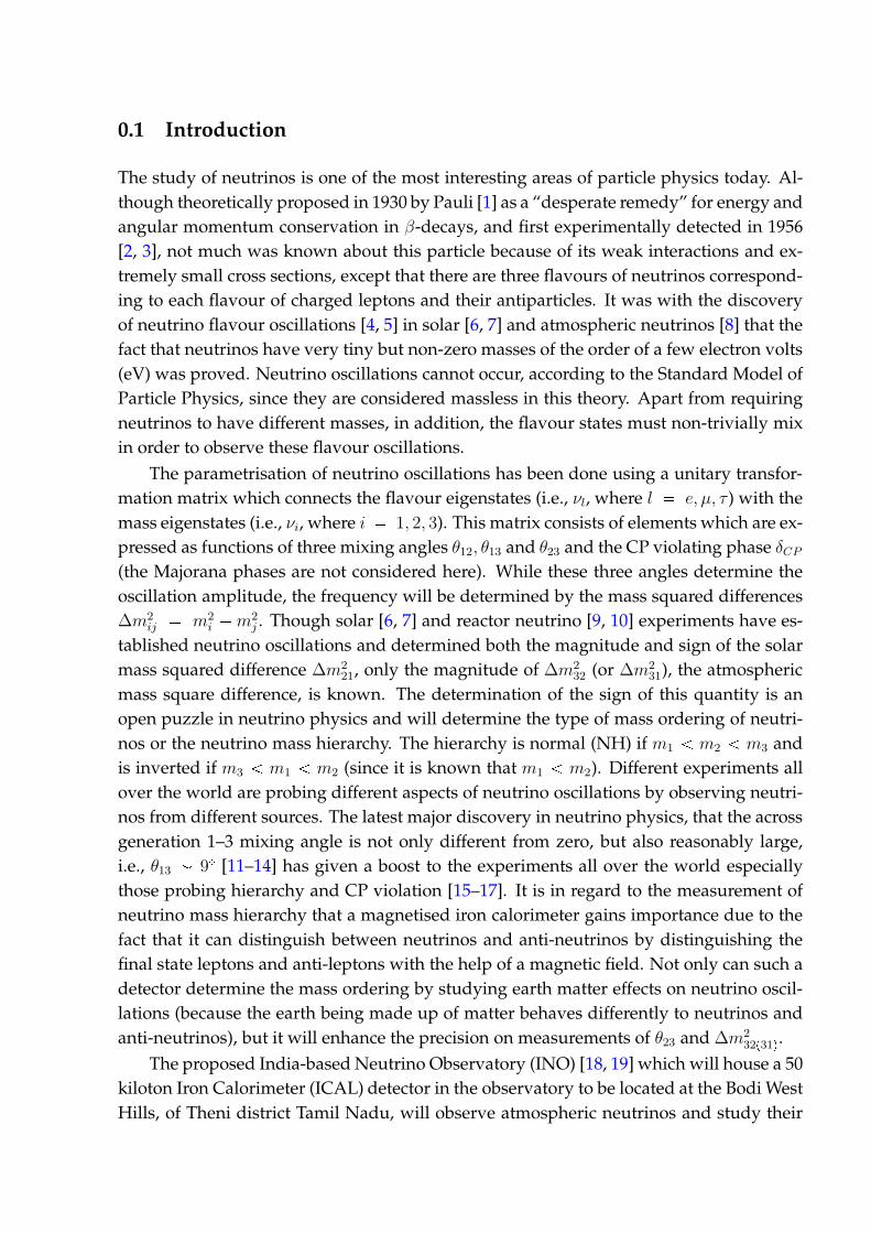
0.1 Introduction

The study of neutrinos is one of the most interesting areas of particle physics today. Al-

though theoretically proposed in 1930 by Pauli [1] as a “desperate remedy” for energy and

angular momentum conservation in β-decays, and first experimentally detected in 1956

[2, 3], not much was known about this particle because of its weak interactions and ex-

tremely small cross sections, except that there are three flavours of neutrinos correspond-

ing to each flavour of charged leptons and their antiparticles. It was with the discovery

of neutrino flavour oscillations [4, 5] in solar [6, 7] and atmospheric neutrinos [8] that the

fact that neutrinos have very tiny but non-zero masses of the order of a few electron volts

(eV) was proved. Neutrino oscillations cannot occur, according to the Standard Model of

Particle Physics, since they are considered massless in this theory. Apart from requiring

neutrinos to have different masses, in addition, the flavour states must non-trivially mix

in order to observe these flavour oscillations.

The parametrisation of neutrino oscillations has been done using a unitary transfor-

mation matrix which connects the flavour eigenstates (i.e., νl, where l e, µ, τ ) with the

mass eigenstates (i.e., νi, where i 1, 2, 3). This matrix consists of elements which are ex-

pressed as functions of three mixing angles θ12, θ13 and θ23 and the CP violating phase δCP(the Majorana phases are not considered here). While these three angles determine the

oscillation amplitude, the frequency will be determined by the mass squared differences

∆m2ij m2

i m2j . Though solar [6, 7] and reactor neutrino [9, 10] experiments have es-

tablished neutrino oscillations and determined both the magnitude and sign of the solar

mass squared difference ∆m221, only the magnitude of ∆m2

32(or ∆m2

31), the atmospheric

mass square difference, is known. The determination of the sign of this quantity is an

open puzzle in neutrino physics and will determine the type of mass ordering of neutri-

nos or the neutrino mass hierarchy. The hierarchy is normal (NH) if m1 m2 m3 and

is inverted if m3 m1 m2 (since it is known that m1 m2). Different experiments all

over the world are probing different aspects of neutrino oscillations by observing neutri-

nos from different sources. The latest major discovery in neutrino physics, that the across

generation 1–3 mixing angle is not only different from zero, but also reasonably large,

i.e., θ13 9 [11–14] has given a boost to the experiments all over the world especially

those probing hierarchy and CP violation [15–17]. It is in regard to the measurement of

neutrino mass hierarchy that a magnetised iron calorimeter gains importance due to the

fact that it can distinguish between neutrinos and anti-neutrinos by distinguishing the

final state leptons and anti-leptons with the help of a magnetic field. Not only can such a

detector determine the mass ordering by studying earth matter effects on neutrino oscil-

lations (because the earth being made up of matter behaves differently to neutrinos and

anti-neutrinos), but it will enhance the precision on measurements of θ23 and ∆m2

32p31q.

The proposed India-based Neutrino Observatory (INO) [18, 19] which will house a 50

kiloton Iron Calorimeter (ICAL) detector in the observatory to be located at the Bodi West

Hills, of Theni district Tamil Nadu, will observe atmospheric neutrinos and study their

vi

oscillations. These atmospheric neutrinos produced in the atmosphere by the decay of

secondary cosmic rays in the upper atmosphere are in the few GeV energy range (from

0.1 GeV to 500 GeV; with flux falling rapidly as the energy increases). The ICAL detector

will consist of three modules of dimension 16 m 16 m 14.45m; each module will have

magnetic coils to produce a central field of about 1.5 Tesla. There will be 151 horizontal

layers of iron plates of thickness 5.6 cm, stacked one above the other with a separation of

4 cm, interspersed with glass resistive plate chambers (RPCs) in the gaps. The iron plates

will both act as the passive detector with which the neutrinos (anti-neutrinos) interact

and also serve to make the detector an electromagnet. RPCs which are the active detec-

tor elements will detect the charged particles produced in the neutrinos (anti-neutrinos)

interactions with iron. The charged current interactions of νµ and νµ are of main interest

in ICAL and the detector is optimised for the detection of µ and µ, distinguished from

each other by means of the magnetic field. In addition to the charged leptons, hadrons

are also produced in the interactions which can be used as observables in the neutrino os-

cillation studies, thus adding to the sensitivity to oscillation parameters. The ICAL may

also probe new physics such as CPT violation, help in the search for sterile neutrinos and

magnetic monopoles. It opens a possibility of probing dark matter too.

This synopsis gives a brief account of the simulation studies conducted on the re-

sponse of the ICAL to hadrons; in particular, the sensitivity of ICAL to determine the

energy [20, 21] and direction of hadrons propagating through it. These sensitivities, as

well as the response of ICAL to muons (which have been studied independently [22])

have been used to conduct a detailed physics simulation on the reach of ICAL with re-

spect to some of the neutrino oscillation parameters including mass hierarchy, ∆m232 and

θ23.

0.2 Energy and direction resolutions of hadrons in ICAL

This section describes the GEANT-4 [23] based simulation studies to calibrate the hadron

response of ICAL. There can be more than one hadron in a single interaction. Since there

is no information on the energy deposition in the RPC, individual hadrons cannot be

separated and reconstructed calorimetrically. The only observable that can be used is the

number of hits in the hadron shower. The origin of these hadrons is briefly described first.

0.2.1 Neutrino interaction processes

The three broad categories through which νµ and νµ interact with iron are, quasi-elastic

(QE), resonance (RES) and deep inelastic scattering (DIS). There can be charged current

(CC) as well as neutral current (NC) interactions, but the main interest is on charged

current interactions of νµ and νµ which will produce µ and hadrons in the final state.

Quasi elastic processes are dominant in the sub-GeV energy range. They do not have any

hadrons in the final state in addition to the recoil nucleons. With increase in energy, RES

0.2. ENERGY AND DIRECTION RESOLUTIONS OF HADRONS IN ICAL vii

andDIS become dominant; at a fewGeV, DIS becomes themost dominant one. Resonance

events mostly contain a single pion in the final state (though a very small fraction may

contain multiple pions), whereas DIS events produce multiple hadrons. Neutrino CC and

NC events have been generated for these studies using the NUANCE neutrino generator

[24]. To reconstruct the energy and direction of a neutrino the energies and directions

of the final state particles have to be reconstructed. Unlike muons (which are minimum

ionising particles) which leave a clean track in the detector, hadrons in ICAL only shower.

The only way to reconstruct hadrons in ICAL is to make use of the shower hit informa-

tion, the number of hits coding for net energy and the hit position for net direction of all

hadrons in the shower.

0.2.2 Hadron energy resolution

The study of the energy resolution of single pions propagated in the ICAL detector sim-

ulated in GEANT-4 was first done. Since ICAL consists of two sets of strips in the X and

Y directions arranged perpendicular to each other, the px, y, zq positions of the hits along

with the number of hits in both X direction and Y direction separately can be obtained.

To avoid false double counting of hits (ghost hits), the maximum of the hits out of those

produced inX and Y layers are taken for each event. The simulation studies are confined

to single pions only, since pions constitute the majority of hadrons ( 80%) in the shower

and it has been observed through simulations of π, π0, K, K0 and protons of fixed en-

ergies propagated through ICAL, that the detector cannot distinguish between different

hadrons. The number of hits can be calibrated to the energy of the pion which gives the

distribution. The mean number of hits increases with energy and is related to the pion

energy by the relation :

npEq n0 r1 exp pEE0qs , (1)

where n0 and E0 are constants. In the 1–15 GeV energy range, the fits yield n0 53 and

E0 24.25 GeV. In the limit E ! E0, the relation becomes linear; the hadron energy

resolution can then be defined as :

σE ∆EE ∆npEqnpEq, (2)

since energy is calibrated to the number of hits. The energy resolution is obtained by

fitting σE according to :

σ

E

a2

E b2 , (3)

where a and b are constants.

To determine the energy resolution, both the arithmetic mean and sigma of the actual

distribution or the mean and sigma obtained from a functional fit to the hit distribution

can be used. It has been observed that the hit distributions are not symmetric at low en-

ergies especially below 6 GeV. Hence a Gaussian function cannot fit below this energy.

viii

E (GeV)2 4 6 8 10 12 14

vav

/Mea

nva

vσ

0.4

0.5

0.6

0.7

0.8

0.9

/ ndf 2χ 165.7 / 55

a 0.004552± 0.863

b 0.001707± 0.2801

/ ndf 2χ 165.7 / 55

a 0.005± 0.863

b 0.002± 0.280

vav/Meanvavσ

2+bE2a

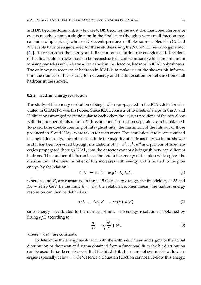
Figure 1: Energy resolution of fixed energy single pions deterined through fits to a Vavilov distribution asa function of incident pion energy in GeV, fitted with Eq. 3.

On the other hand, Vavilov distribution function [25, 26], which estimates the energy loss

of particles propagating in moderately thick absorbers like iron fits well to the hadron

hit distribution in ICAL which is asymmetric at lower energies. With the increase in en-

ergy these become Gaussian in shape. The Vavilov distribution is characterised by two

parameters κ and β and approximates to a Landau distribution when κ ¤ 0.05 and to a

Gaussian for κ ¥ 10. The mean and sigma,Meanvav and σvav are then used in the estima-

tion of single pion energy resolution using Eq. 3. The energy resolution as a function of

the pion energy is shown in Fig. 1. The energy resolution varies from 91.7% at 1 GeV to

35.5% at 15 GeV. This work is reported in detail in Ref. [20].

Energy resolution of hadrons as a function of iron plate thickness

The default plate thickness in ICAL is 5.6 cm and the results discussed in Section 3.5

above were obtained with this default geometry. However it is interesting to study the

effect of changing plate thickness on hadron energy resolution since the hadron energy

plays a crucial role in enhancing the sensitivity of ICAL to oscillation parameters [27] and

any improvement in the hadron energy resolution will further improve ICAL’s physics

potential. GEANT-4 based simulation studies [21] of fixed energy single pions propa-

gating from vertices randomised in the central region of ICAL were conducted in this

regard, using eleven different plate thicknesses including the default value 5.6 cm. The

plate thicknesses used were 1.5 cm to 5 cm in steps of 0.5 cm, 5.6 cm, 6 cm and 8 cm re-

spectively, in the hadron energy range 2–15 GeV. It is seen that the mean number of hits

increases with increase in energy and decrease in thickness; thus the largest number of

hits are for 1.5 cm plate at a given energy. The width of the distribution also follows the

same trend, with the histograms becoming more and more symmetric (Gaussian) with

smaller thickness and increasing energy. Since the study is confined to the effect of vary-

0.2. ENERGY AND DIRECTION RESOLUTIONS OF HADRONS IN ICAL ix

ing thickness on energy resolution, the arithmetic mean and RMS, Meanarith and σarith

have been used to estimate the responses. The square of Eq. 3 has been used for this

analysis, since it is linear in 1E; i.e.,

σ

E

2

a2

E b2, (4)

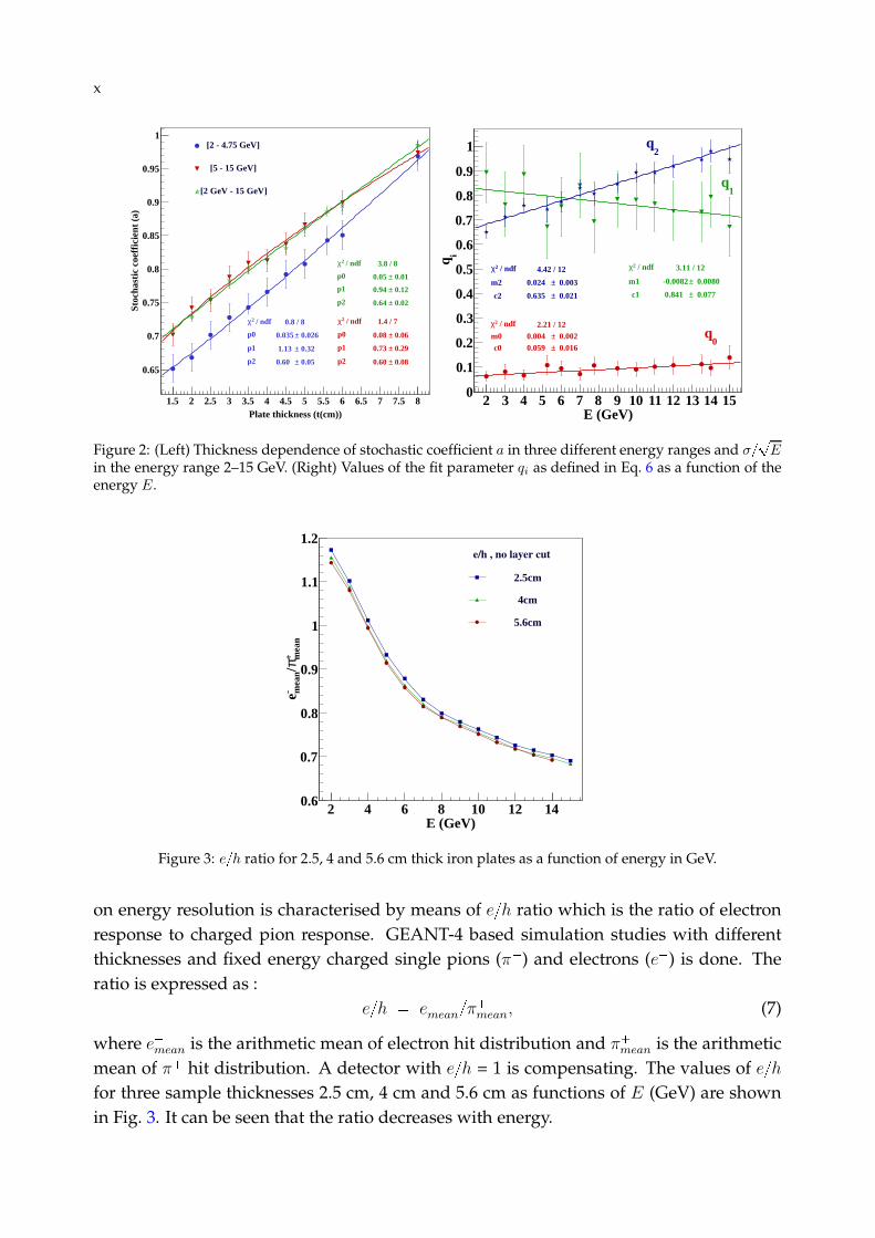
where a is the stochastic coefficient and b is a constant. The plots of pσarithMeanarithq2

vs 1E fitted with Eq. 4, give the values of a and b for various thicknesses. In the energy

range 2–15 GeV, a varies from 0.71 to 0.99 and b from 0.23 to 0.29 respectively.

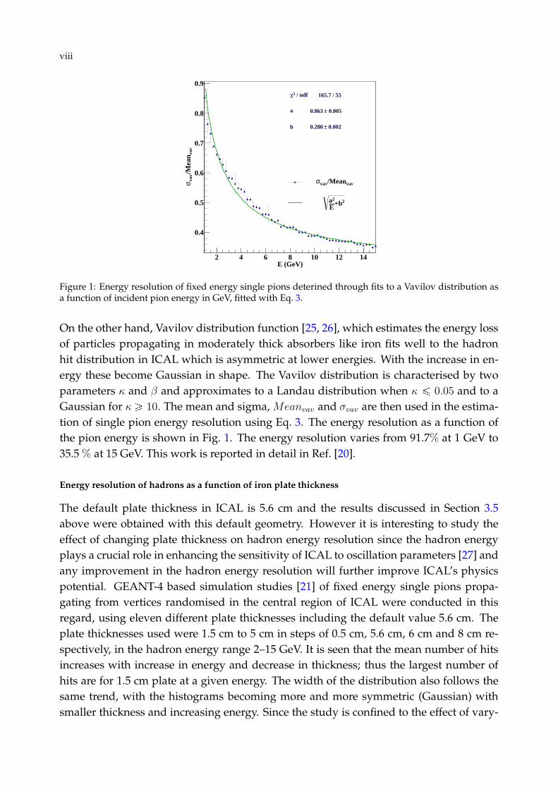
Thickness dependence can be parametrised in two ways, one in which the thickness

dependence is attributed to stochastic coefficient a only and the other in which the de-

pendence of the entire width is studied. The first takes the standard form :

aptq p0tp1 p2, (5)

where p2 is the limiting resolution of hadrons for finite energy in the very small thickness

limit. In the 2–15 GeV range, the values of pi, i 0, 1, 2, are 0.05, 0.94 and 0.64 respec-

tively. This implies that there is always a residual resolution of hadrons due to the nature

of strong interactions, detector geometry and other systematic effects even if the plate

thickness is made infinitesimally small. It can be seen that the dependence is not a?

t

one as shown by the value of p1. The coefficient p0 is small and p2 being fairly large again

emphasises the effect of residual resolution on the energy response. Stochastic coefficient

a vs plate thickness t (cm), in three different energy range 2–4.75 GeV (low energy), 5–15

GeV (high energy) and 2–15 GeV is shown in Fig. 2. In the alternative approach, the a fit

to σ?

E is done with the equation:

σ?

E q0tq1 q2. (6)

In the 2–15 GeV energy range, fit parameter q1, the exponent of plate thickness decreases

from 0.9 to 0.66, whereas q0 increases from 0.06 to 0.14 with energy. The constant q2increases from 0.65 to 0.98 with energy and this behaviour is similar to that of the the

previous approach.

Direction dependence of energy resolution and its thickness dependence has also

been studied. As expected the resolution is worse in the horizontal direction and gets

better as the direction becomes more vertical, but worse in the most vertical direction

contrary to expectation, due to the presence of support structures in this direction and

detector specific geometry.

e/h ratio in ICAL

Neutral pions can also be produced in these interactions and they behave differently from

charged pions since the former decay electromagnetically. The effect of neutral hadrons

x

Plate thickness (t(cm))1.5 2 2.5 3 3.5 4 4.5 5 5.5 6 6.5 7 7.5 8

Sto

chas

tic c

oeffi

cien

t (a)

0.65

0.7

0.75

0.8

0.85

0.9

0.95

1

/ ndf 2χ 0.789 / 8

p0 0.02607± 0.03473

p1 0.3169± 1.13

p2 0.04741± 0.5987

/ ndf 2χ 0.8 / 8

p0 0.026± 0.035

p1 0.32± 1.13

p2 0.05± 0.60

/ ndf 2χ 1.401 / 7

p0 0.06436± 0.08097

p1 0.2866± 0.7337

p2 0.08471± 0.5993

/ ndf 2χ 1.4 / 7

p0 0.06± 0.08

p1 0.29± 0.73

p2 0.08± 0.60

/ ndf 2χ 3.8 / 8

p0 0.01± 0.05

p1 0.12± 0.94

p2 0.02± 0.6389

/ ndf 2χ 3.8 / 8

p0 0.01± 0.05

p1 0.12± 0.94

p2 0.02± 0.64

[2 - 4.75 GeV]

[5 - 15 GeV]

[2 GeV - 15 GeV]

E (GeV)2 3 4 5 6 7 8 9 10 11 12 13 14 15

iq

0

0.1

0.2

0.3

0.4

0.5

0.6

0.7

0.8

0.9

1

/ ndf 2χ 2.21 / 12m1 0.002± 0.004 c1 0.016± 0.059

/ ndf 2χ 2.21 / 12m0 0.002± 0.004 c0 0.016± 0.059

/ ndf 2χ 3.11 / 12

m2 0.0080± -0.0082

c2 0.077± 0.841

/ ndf 2χ 3.11 / 12

m1 0.0080± -0.0082

c1 0.077± 0.841

/ ndf 2χ 4.42 / 12

m3 0.003± 0.024

c3 0.021± 0.635

/ ndf 2χ 4.42 / 12

m2 0.003± 0.024

c2 0.021± 0.635

0q

1q

2q

Figure 2: (Left) Thickness dependence of stochastic coefficient a in three different energy ranges and σ?

E

in the energy range 2–15 GeV. (Right) Values of the fit parameter qi as defined in Eq. 6 as a function of theenergy E.

E (GeV)2 4 6 8 10 12 14

mea

n+ π/

mea

n- e

0.6

0.7

0.8

0.9

1

1.1

1.2 e/h , no layer cut

2.5cm

4cm

5.6cm

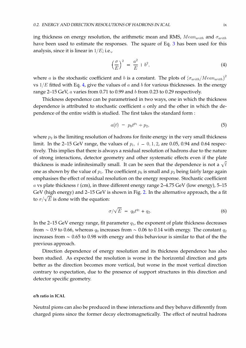
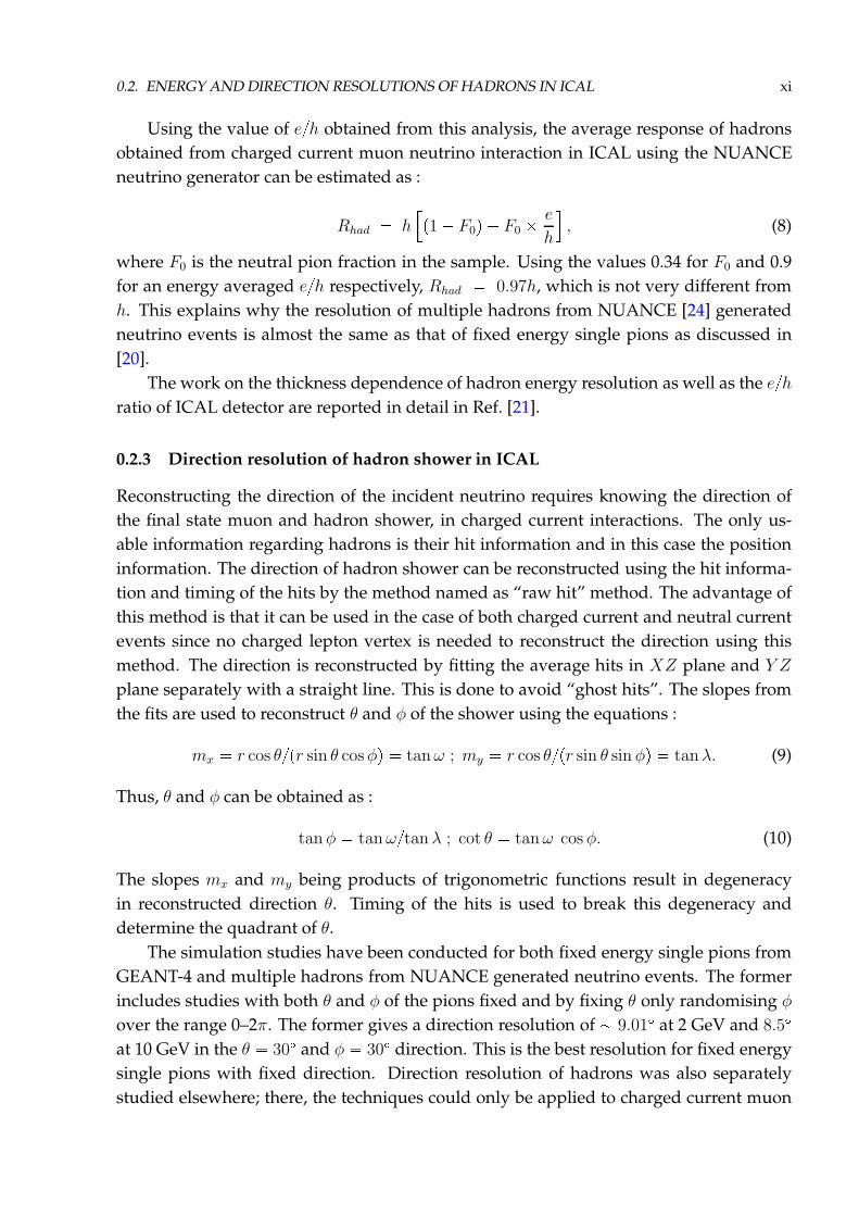
Figure 3: eh ratio for 2.5, 4 and 5.6 cm thick iron plates as a function of energy in GeV.

on energy resolution is characterised by means of eh ratio which is the ratio of electron

response to charged pion response. GEANT-4 based simulation studies with different

thicknesses and fixed energy charged single pions (π) and electrons (e) is done. The

ratio is expressed as :

eh emeanπ

mean, (7)

where emean is the arithmetic mean of electron hit distribution and πmean is the arithmetic

mean of π hit distribution. A detector with eh = 1 is compensating. The values of eh

for three sample thicknesses 2.5 cm, 4 cm and 5.6 cm as functions of E (GeV) are shown

in Fig. 3. It can be seen that the ratio decreases with energy.

0.2. ENERGY AND DIRECTION RESOLUTIONS OF HADRONS IN ICAL xi

Using the value of eh obtained from this analysis, the average response of hadrons

obtained from charged current muon neutrino interaction in ICAL using the NUANCE

neutrino generator can be estimated as :

Rhad h

p1 F0q F0

e

h

, (8)

where F0 is the neutral pion fraction in the sample. Using the values 0.34 for F0 and 0.9

for an energy averaged eh respectively, Rhad 0.97h, which is not very different from

h. This explains why the resolution of multiple hadrons from NUANCE [24] generated

neutrino events is almost the same as that of fixed energy single pions as discussed in

[20].

The work on the thickness dependence of hadron energy resolution as well as the eh

ratio of ICAL detector are reported in detail in Ref. [21].

0.2.3 Direction resolution of hadron shower in ICAL

Reconstructing the direction of the incident neutrino requires knowing the direction of

the final state muon and hadron shower, in charged current interactions. The only us-

able information regarding hadrons is their hit information and in this case the position

information. The direction of hadron shower can be reconstructed using the hit informa-

tion and timing of the hits by the method named as “raw hit” method. The advantage of

this method is that it can be used in the case of both charged current and neutral current

events since no charged lepton vertex is needed to reconstruct the direction using this

method. The direction is reconstructed by fitting the average hits in XZ plane and Y Z

plane separately with a straight line. This is done to avoid “ghost hits”. The slopes from

the fits are used to reconstruct θ and φ of the shower using the equations :

mx r cos θpr sin θ cosφq tanω ; my r cos θpr sin θ sin φq tanλ. (9)

Thus, θ and φ can be obtained as :

tanφ tanωtanλ ; cot θ tanω cos φ. (10)

The slopes mx and my being products of trigonometric functions result in degeneracy

in reconstructed direction θ. Timing of the hits is used to break this degeneracy and

determine the quadrant of θ.

The simulation studies have been conducted for both fixed energy single pions from

GEANT-4 and multiple hadrons from NUANCE generated neutrino events. The former

includes studies with both θ and φ of the pions fixed and by fixing θ only randomising φ

over the range 0–2π. The former gives a direction resolution of 9.01 at 2 GeV and 8.5

at 10 GeV in the θ 30 and φ 30 direction. This is the best resolution for fixed energy

single pions with fixed direction. Direction resolution of hadrons was also separately

studied elsewhere; there, the techniques could only be applied to charged current muon

xii

events since it was crucial to know the vertex of interaction (obtained from the muon

track). The work on hadron direction resoltion will be reported in Ref. [28].

0.3 Physics simulation studies: An improved analysis

Earlier oscillation analyses of ICAL physics, both with observed muon energy and direc-

tion pEµ, cos θµq [29, 30] and with muon momentum and hadron energy pEµ, cos θµ, E1

hadq

[27] have been conducted only in the observed muon energy range of 1–11 GeV (0.8–10.8

GeV in [29, 30]) and including 10 systematic errors (pulls). These have been named as

‘2D’ and ‘3D’ methods. It is interesting to see the effect of adding higher energy bins in

the observed muon energy since ICAL is looking at atmospheric neutrinos. Even though

the fluxes are small at these energies, it has been seen in the study discussed here that the

higher energy events contribute significantly to the enhancement of sensitivity to oscilla-

tion parameters. The analysis is briefly discussed here.

0.3.1 A brief description of the analysis

Since real data is not available, “data” has been simulated and used for analysis. Unoscil-

lated events for 1000 years are generated using NUANCE neutrino generator and scaled

down to the required number of years to reduce the effect of fluctuations in theory. The

analysis procedure is described briefly here.

1. Generation of events : The events of interest, viz., charged current muon neutrino

(anti-neutrino) (CC νµ and CC νµ) events are generated using NUANCE neutrino

generator version 3.5 [24]. Unoscillated events are generated according to the atmo-

spheric neutrino flux at Super Kamiokande (SK) site as calculated in Honda 3D flux

table. A very large set of data sample is generated, here for 1000 years, to reduce

statistical fluctuations, and then this sample is scaled down to the required number

of years for which the analysis has to be carried out.

2. Inclusion of detector responses, efficiencies and oscillations : The detector responses

for muon momentum and direction and hadron energy in the central region of the

detector, given according to the look-up table prepared by INO collaboration [20, 22]

for these quantities have been used for the analysis. The efficiency of detecting each

event has been taken as the efficiency with which a muon is reconstructed and this

is the same for both 2D and 3D analysis. Charge identification (CID) efficiency has

been incorporated to analyse neutrino and anti-neutrino events separately. Events

are smeared according to the detector response and are binned into the observed

bins. Oscillations are applied to each event, using a 3-flavour oscillation code that

accounts in detail for the Earth Matter (PREM) profile [31]. It should be noted that

the oscillations are applied on an event-by-event basis.

0.3. PHYSICS SIMULATION STUDIES: AN IMPROVED ANALYSIS xiii

3. Binning scheme : There are two different analyses, one in which the events are

binned in observed muon energy and direction only pEµ, cos θµq which is called the

2D analysis and the other in which the bins are in observed Eµ, cos θµ, E1

had which is

the 3D analysis. The observed muon energy has 15 bins from 0.5–25 GeV as com-

pared to the old 1–11 GeV analyses. The observed muon direction cos θµ ranges from

1 to 1 in 21 bins and there are 4 hadron energy bins from 0–15 GeV. All bins are

non-uniform and are separate for each polarity of muon.

4. χ2 analysis and addition of extra pull : The χ2 analysis is done by determining the

χ2 corresponding to each observed bin mentioned above. Since neutrino detection

experiments are low counting experiments, Poissonian χ2 is used to take into account

the small number of events per bin. Five systematic errors have been used for each

polarity of muon in the analysis using method of pulls [32]: 20% flux normalisation

error, 10% cross section error, 5% tilt error, 5% zenith angle error and 5% overall

systematics. An extra pull is added in the current analysis as a constraint on the

νµ-νµ flux ratio which is also found to enhance the physics potential of ICAL.

In the case with just 10 pulls, the Poissonian χ2 is a sum of the individual χ2s for µ

and µ events:

χ2

minξl

NEobsµ¸

i1

Ncos θobsµ¸

j1

NE1obshad¸

k1

2

T

ijpkqD

ijpkq

D

ijpkqln

T

ijpkq

D

ijpkq

5¸

l1

ξ2l,

(11)

where T

ijpkq T 0

ijpkq

1°

5

l1πl

ijpkqξl

is the number of theory (expected) events

in each bin with systematic errors, T 0

ijpkqis the number of theory (expected) events in

each bin without systematic errors, D

ijpkqis the number of “data” (observed) events

in each bin, i, j, k are the observed bin indices, ξl are the pulls, πl are the systematic

uncertainties with l 1, . . . , 5.

For the case when the additional (ξ6) pull is included, the χ2 is no longer a sum

because of the constraint between µ and µ events:

χ2 minξ

l,ξ6

NEobsµ¸

i1

Ncos θobsµ¸

j1

NE1obshad¸

k1

2

T

ijpkqD

ijpkq

D

ijpkqln

T

ijpkq

D

ijpkq

2

T

ijpkqD

ijpkq

D

ijpkqln

T

ijpkq

D

ijpkq

5

l1

ξ2l

5

l1

ξ2l ξ26, (12)

where ‘D’s represent the simulated “data” events as before and theory predicts the

xiv

observed (T ) events as

T

ijpkq T 0

ijpkq

1

5¸

l1

πl

ijpkqξl π6ξ6

,

T

ijpkq T 0

ijpkq

1

5¸

l1

πl

ijpkqξl π6ξ6

.

Here ξ6 is the 11th pull and constraints the µ : µ ratio with π6 = 2.5%. Since the new

pull acts as a constraint to the ΦνµΦνµ ratio, the expressions for χ2 from neutrino and

anti-neutrino events cannot be written separately.

An 8% prior (at 1σ) on sin2 2θ13 is also added to obtain the total χ2. Hence the total

chisq is given as :

χ2

ICAL χ2

χ2

χ2

prior, (13)

when there are 10 pulls only and

χ2

ICAL χ2 χ2

prior, (14)

when there are 11 pulls. A marginalisation over all the pull variables and over the

allowed 3σ regions of the oscillation parameters relevant for atmospheric neutrinos

has been carried out to obtain the results.

0.3.2 Precision measurement of θ23 and |∆m2

eff |

The relative precision achieved on a parameter λ (here λ being sin2 θ23 or ∆m2

eff ) at 1σ is

expressed as :

ppλq λmax2σ λmin2σ

4λtrue, (15)

where λmax2σ and λmin2σ are the maximum and minimum allowed values of λ at 2σ;

λtrue is the true choice. Here the effective mass squared difference observed in atmo-

spheric neutrino experiments is defined as :

∆m2

eff ∆m231∆m2

21pcos2 θ12 cos δCP sin θ13 sin 2θ12 tan θ23q.

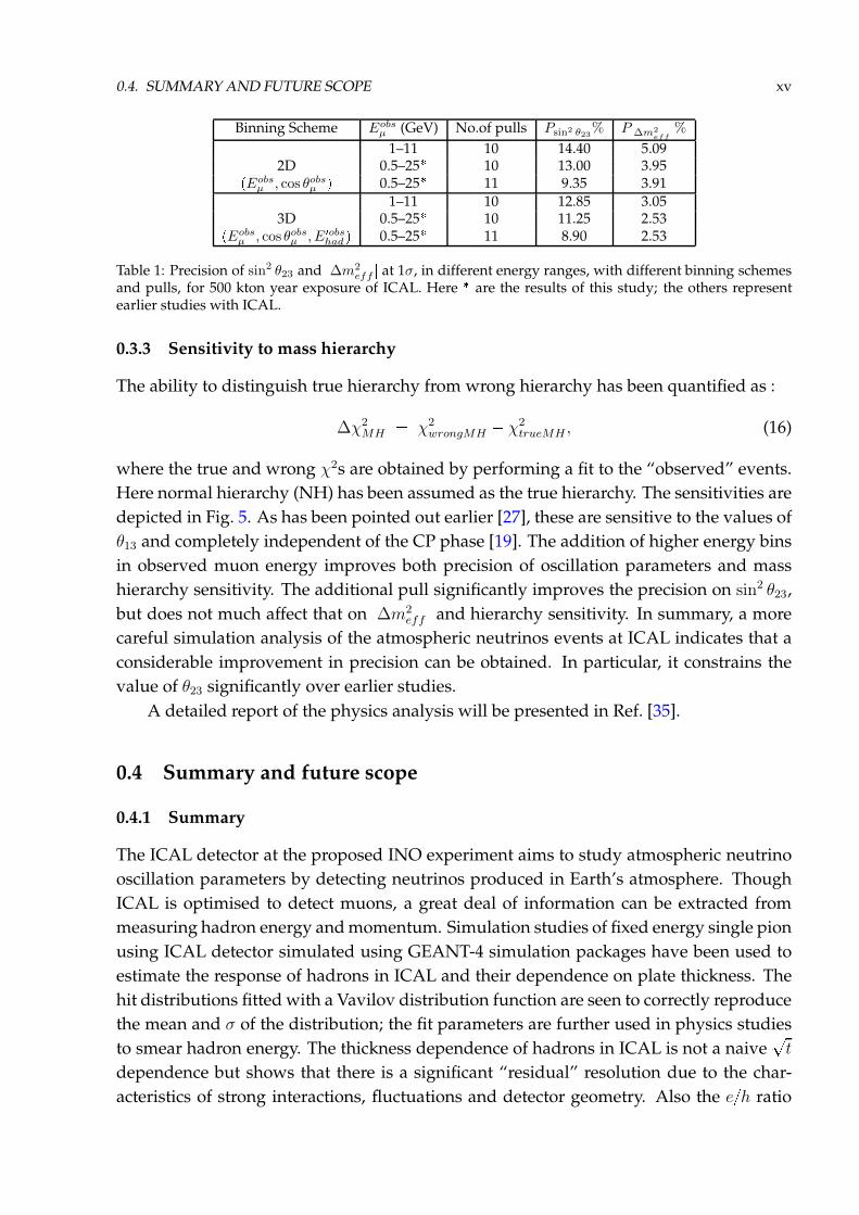
The precisions achievable by ICAL with 500 kton year exposure (10 years of run) in dif-

ferent scenarios are listed in Table 1. The main observation is that the precision measure-

ments improve with the current analysis and is significant in the case of sin2 θ23 as can

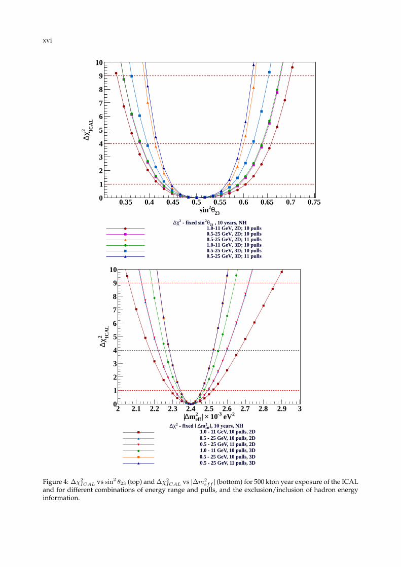
be seen from Table 1. The plots for ∆χ2ICAL vs sin2 θ23 and |∆m2

eff | are shown in Fig. 4

for different analyses. The improvement in the precision for ICAL can be seen. Other

currently running main experiments measuring the precision of atmospheric neutrino

oscillation parameters are MINOS [33] and T2K [34]. This improvement in the precision

will contribute to the global analysis of this parameter and related quantities.

0.4. SUMMARY AND FUTURE SCOPE xv

Binning Scheme Eobsµ (GeV) No.of pulls Psin2 θ23% P

|∆m2

eff|

%

1–11 10 14.40 5.092D 0.5–25 10 13.00 3.95

pEobsµ , cos θobsµ q 0.5–25 11 9.35 3.91

1–11 10 12.85 3.053D 0.5–25 10 11.25 2.53

pEobsµ , cos θobsµ , E1obs

had q 0.5–25 11 8.90 2.53

Table 1: Precision of sin2 θ23 and |∆m2

eff | at 1σ, in different energy ranges, with different binning schemesand pulls, for 500 kton year exposure of ICAL. Here are the results of this study; the others representearlier studies with ICAL.

0.3.3 Sensitivity to mass hierarchy

The ability to distinguish true hierarchy from wrong hierarchy has been quantified as :

∆χ2

MH χ2

wrongMH χ2

trueMH , (16)

where the true and wrong χ2s are obtained by performing a fit to the “observed” events.

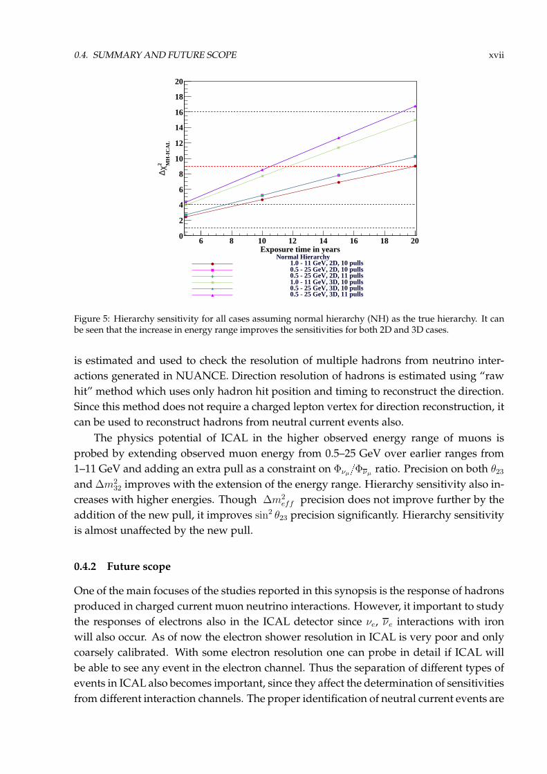
Here normal hierarchy (NH) has been assumed as the true hierarchy. The sensitivities are

depicted in Fig. 5. As has been pointed out earlier [27], these are sensitive to the values of

θ13 and completely independent of the CP phase [19]. The addition of higher energy bins

in observed muon energy improves both precision of oscillation parameters and mass

hierarchy sensitivity. The additional pull significantly improves the precision on sin2 θ23,

but does not much affect that on |∆m2

eff | and hierarchy sensitivity. In summary, a more

careful simulation analysis of the atmospheric neutrinos events at ICAL indicates that a

considerable improvement in precision can be obtained. In particular, it constrains the

value of θ23 significantly over earlier studies.

A detailed report of the physics analysis will be presented in Ref. [35].

0.4 Summary and future scope

0.4.1 Summary

The ICAL detector at the proposed INO experiment aims to study atmospheric neutrino

oscillation parameters by detecting neutrinos produced in Earth’s atmosphere. Though

ICAL is optimised to detect muons, a great deal of information can be extracted from

measuring hadron energy andmomentum. Simulation studies of fixed energy single pion

using ICAL detector simulated using GEANT-4 simulation packages have been used to

estimate the response of hadrons in ICAL and their dependence on plate thickness. The

hit distributions fitted with a Vavilov distribution function are seen to correctly reproduce

the mean and σ of the distribution; the fit parameters are further used in physics studies

to smear hadron energy. The thickness dependence of hadrons in ICAL is not a naive?

t

dependence but shows that there is a significant “residual” resolution due to the char-

acteristics of strong interactions, fluctuations and detector geometry. Also the eh ratio

xvi

23θ2sin0.35 0.4 0.45 0.5 0.55 0.6 0.65 0.7 0.75

ICA

L

2 χ∆

0

1

2

3

4

5

6

7

8

9

10

, 10 years, NH23θ2 - fixed sin2χ∆1.0-11 GeV, 2D; 10 pulls0.5-25 GeV, 2D; 10 pulls0.5-25 GeV, 2D; 11 pulls1.0-11 GeV, 3D; 10 pulls0.5-25 GeV, 3D; 10 pulls0.5-25 GeV, 3D; 11 pulls

2 eV-3 10×| eff2m∆|

2 2.1 2.2 2.3 2.4 2.5 2.6 2.7 2.8 2.9 3

ICA

L2 χ

∆

0

1

2

3

4

5

6

7

8

9

10

|, 10 years, NH2eff

m∆ fixed |2χ∆1.0 - 11 GeV, 10 pulls, 2D0.5 - 25 GeV, 10 pulls, 2D0.5 - 25 GeV, 11 pulls, 2D1.0 - 11 GeV, 10 pulls, 3D0.5 - 25 GeV, 10 pulls, 3D0.5 - 25 GeV, 11 pulls, 3D

Figure 4: ∆χ2ICAL vs sin2 θ23 (top) and∆χ2

ICAL vs |∆m2eff | (bottom) for 500 kton year exposure of the ICAL

and for different combinations of energy range and pulls, and the exclusion/inclusion of hadron energyinformation.

0.4. SUMMARY AND FUTURE SCOPE xvii

Exposure time in years6 8 10 12 14 16 18 20

MH

-IC

AL

2 χ∆

0

2

4

6

8

10

12

14

16

18

20

Normal Hierarchy1.0 - 11 GeV, 2D, 10 pulls0.5 - 25 GeV, 2D, 10 pulls0.5 - 25 GeV, 2D, 11 pulls1.0 - 11 GeV, 3D, 10 pulls0.5 - 25 GeV, 3D, 10 pulls0.5 - 25 GeV, 3D, 11 pulls

Figure 5: Hierarchy sensitivity for all cases assuming normal hierarchy (NH) as the true hierarchy. It canbe seen that the increase in energy range improves the sensitivities for both 2D and 3D cases.

is estimated and used to check the resolution of multiple hadrons from neutrino inter-

actions generated in NUANCE. Direction resolution of hadrons is estimated using “raw

hit” method which uses only hadron hit position and timing to reconstruct the direction.

Since this method does not require a charged lepton vertex for direction reconstruction, it

can be used to reconstruct hadrons from neutral current events also.

The physics potential of ICAL in the higher observed energy range of muons is

probed by extending observed muon energy from 0.5–25 GeV over earlier ranges from

1–11 GeV and adding an extra pull as a constraint on ΦνµΦνµ ratio. Precision on both θ23and∆m2

32 improves with the extension of the energy range. Hierarchy sensitivity also in-

creases with higher energies. Though |∆m2

eff | precision does not improve further by the

addition of the new pull, it improves sin2 θ23 precision significantly. Hierarchy sensitivity

is almost unaffected by the new pull.

0.4.2 Future scope

One of the main focuses of the studies reported in this synopsis is the response of hadrons

produced in charged current muon neutrino interactions. However, it important to study

the responses of electrons also in the ICAL detector since νe, νe interactions with iron

will also occur. As of now the electron shower resolution in ICAL is very poor and only

coarsely calibrated. With some electron resolution one can probe in detail if ICAL will

be able to see any event in the electron channel. Thus the separation of different types of

events in ICAL also becomes important, since they affect the determination of sensitivities

from different interaction channels. The proper identification of neutral current events are

xviii

also important since they can impact sterile neutrino searches. It is also important to have

studies on newer algorithms to determine hadron shower direction in the detector. The

effect of reducing strip width on the azimuthal angle (φ) determination of hadrons and

its effect on the shower direction measurement has to be probed.

The sensitivity studies of ICAL reported here makes use of the atmospheric neutrino

flux at Super Kamiokande site. The analysis with the neutrino flux at Theni where the

observatory will be located is crucial. These flux tables are just being made available.

Also studies on how the improved precisions and hierarchy sensitivities of ICAL can

impact the global measurement of neutrino oscillation parameters have to be studied in

detail. Sensitivity studies using hadron direction as the fourth observable in the binning

scheme can also be probed. Finally, the significant improvement in θ23 obtained in this

study will surely impact determination of the as-yet unknown octant of this mixing angle.

List of Figures

1 Energy resolution of fixed energy single pions deterined through fits to a

Vavilov distribution as a function of incident pion energy in GeV, fitted

with Eq. 3. viii

2 (Left) Thickness dependence of stochastic coefficient a in three different

energy ranges and σ?

E in the energy range 2–15 GeV. (Right) Values of

the fit parameter qi as defined in Eq. 6 as a function of the energy E. x

3 eh ratio for 2.5, 4 and 5.6 cm thick iron plates as a function of energy in GeV. x

4 ∆χ2ICAL vs sin2 θ23 (top) and ∆χ2

ICAL vs |∆m2

eff | (bottom) for 500 kton year

exposure of the ICAL and for different combinations of energy range and

pulls, and the exclusion/inclusion of hadron energy information. xvi

5 Hierarchy sensitivity for all cases assuming normal hierarchy (NH) as the

true hierarchy. It can be seen that the increase in energy range improves

the sensitivities for both 2D and 3D cases. xvii

1.1 Neutrino mass ordering. Absolute zero of the mass scale is also unknown.

Picture taken from [69]. 8

1.2 Survival probabilities Pµµ and Pµµ (left) and oscillation probabilities Peµand Peµ (right) at Eν = 0.5, 5 and 30 GeV as functions of logpLνEνq, where

Lν is the distance traveled by the neutrino in km and Eν is the neutrino

energy in GeV, for normal hierarchy. It can be seen that matter resonance

occurs at 5 GeV for neutrinos for normal hierarchy. Matter resonance will

occur for anti-neutrinos in inverted hierarchy. One important feature to be

noted is that the range of logpLνEνq spanned varies with neutrino energy.

Hence the low energy 0.5 GeV neutrinos will span an LνEν region from

1.5–4.4 and the highest energy shown in the figure viz, 30 GeV will span a

region -0.3 to 2.6 (with the cos θ ranging from 0–1). 12

1.3 The current global best fit values of neutrino oscillation parameters as given

in [106, 107]. 17

xix

xx LIST OF FIGURES

2.1 Schematic of the ICAL detector. (Left) Three modules of ICAL with coil

slots. The longest axis is the X axis, the axis in the front portion of the

figure is the Y axis and the one which points vertically upwards is the Z

axis. (Right) Zoom of a portion of the detector with 5.6 cm thick iron plates;

support structures are also visible. 23

2.2 Magnetic field map in a single iron plate at z 0 of the ICAL detector. The

length and direction of the flux lines indicate the magnitude and direction

of the field. In the central region, the field is uniform and has a strength of

1.5 T which provides the best reconstruction of muons in this region. 24

2.3 Total cross section per nucleon per unit energy for charged current neu-

trino interaction (left) and anti-neutrino interaction (right) as a function of

energy for an isoscalar target [111]. Both data and theory predictions are

shown. Figures are sourced from [111]. 29

2.4 Schematic of atmospheric neutrino production [112]. 31

2.5 Direction integrated atmospheric neutrino fluxes in different models (left).

Ratios of fluxes of different types of neutrinos as functions of energy (right)

[113–116]. 32

2.6 Atmospheric neutrino flux distributions averaged over azimuthal angles

at three different neutrino energies namely 0.32 GeV, 1 GeV and 3.2 GeV,

as a function of zenith angle at the Super Kamiokande site [117]. The flux

scales are different for different energies. Here cos θ 1 denotes the

up-direction. 34

3.1 A charged current muon netrino interaction in ICAL. The incoming muon

neutrino interacts with the iron in the detector to prodce a final state muon

which gives a long track and hadrons which shower in the detector. The

energy of the hadrons can be expressed as E 1

had Eν Eµ, where Eν is the

energy of the incoming neutrino and Eµ is the final state muon energy. 41

3.2 Distributions of Xhits, Yhits and orighits for a 5 GeV π. 43

3.3 Hit distributions of at different energies (angle averaged) for charged (π)

and neutral pions (π0), kaons (K) and protons propagated from vertices

in the central 2 m 2 m 2 m volume. 43

3.4 Hit distributions of single pions of energy 2.5 GeV (left) and 9 GeV (right)

propagated from vertices randomised in the volume 2 m 2 m 2 m

in the centre of the detector. It can be seen that the distributions are not

symmetric but have long tails. 44

3.5 Arithmetic mean (top left) and sigma (top right) of hit distributions for

π and π at different energies, in 5.6 cm iron. It can be seen that the

quantities are similar for both π and π. The arithmetic means fitted with

both Eq. 3.3 and linear fit are shown in the bottom panels, for π (bottom

left) and π (bottom right) respectively. 45

LIST OF FIGURES xxi

3.6 Hit distributions of 2.5 GeV and 9 GeV π, fitted with Gaussian function.

The distribution being asymmetric at 2.5 GeV is not well approximated

with a Gaussian, whereas at 9 GeV , it is. This can be attributed to the fact

that there are lesser number of hits at lower energy whereas the number of

hits increases as the energy increases. 46

3.7 Resolutions of both π and π in the energy range [1 – 15 GeV] obtained

by fitting (left) σgausMeangaus with Eq. 3.6 and (right) σarithMeanarith with

Eq. 3.6 respectively. It can be seen that Gaussian parameters give worse res-

olution than the arithmetic ones, since the Gaussian doesn’t approximate

the hit distribution well at low energies. It is evident from the left panel

also that Gaussian mean and sigma result in worse energy resolution. 47

3.8 Fit parameters P0, P1, P2, P3 and P4 of the Vavilov fit to the single pion

hit distributions at different energies. From the value of P0 at different

energies, it can be seen that till about 6 GeV the hit distributions are Vavilov

and approximate to Gaussian distribution after that. The fifth parameter P4

is the normalisation factor. 48

3.9 Comparison of Vavilov, arithmetic and Gaussian mean no.of hits (left) and

sigmas (right) of pion hit distributions. The top panel depicts the values in

the energy range [1 – 15 GeV] whereas the middle and bottom panels show

those in the [1 – 5.75 GeV] (lower) and [6 – 15 GeV] (higher) energy ranges

separately. 50

3.10 Energy resolution obtained by fitting σvavMeanvav with Eq. 3.6, in the [1–

15 GeV] energy range. It can be seen that the resolution obtained using

Vavilov mean and sigma is similar to that obtained using the correspond-

ing arithmetic quantities as shown in Fig. 3.7. The full energy range [1 – 15

GeV] can be split up into a lower and higher energy range to consider dif-

ferent processes. Bottom left and right panels show the energy resolutions

in two separate energy ranges namely [1 – 4.75 GeV] which is the lower

energy range and [5 – 15 GeV], the higher energy range respectively. 51

3.11 Hit distributions of 5 GeV single pions (π) in eleven different iron plate

thicknesses. 54

3.12 Left panels (a), (c) and (e) show the mean no.of hits (Meanarith) in the en-

ergy ranges [2 – 15 GeV], [2 – 4.75 GeV] and [5 – 15 GeV] respectively,

whereas the right panels (b), (d) and (f) show σarith in [2 – 15 GeV], [2 – 4.75

GeV] and [5 – 15 GeV] respectively; as functions of pion energy in GeV for

different thicknesses. The Y-axes on the left panel are different. 55

3.13 Plots of pσarithMeanarithq2 vs 1EpGeV q, where E is the pion energy in

GeV, in the low energy range [2 – 4.75 GeV], for all thicknesses. 56


GeV, in the high energy range [5 – 15 GeV], for all thicknesses. 57

xxii LIST OF FIGURES


GeV, in the high energy range [2 – 15 GeV], for all thicknesses. 58

3.16 Stochastic coefficient a obtained from analysis in energy range [2 – 4.75

GeV], [5 – 15 GeV], [2 – 15 GeV] versus plate thickness t in cm, fitted with

Eq. 3.8. 60

3.17 Variation of the parameters qi obtained by fitting σ?

E to Eq. (3.10) in the

energy range 2–15 GeV. The linear fits through the points indicate the E

dependence for each parameter qi, i 0, 1, 2. 61

3.18 Mean hits and widths of the hit distributions for the default 5.6 cm thick

iron plate in different cos θ bins. 62

3.19 Energy response of a 5 GeV pion in different incident cos θ bins of the pion

as a function of iron plate thicknesses (t in cm). 63

3.20 Left panels (a), (c) and (e) show the energy resolution (pσarithMeanarithq2)

as a function of 1EpGeV q in various cos θ bins for the default iron thickness

of 5.6 cm, in the three different energy ranges [2 – 4.75 GeV], [5 – 15 GeV]

and [2 – 15 GeV] energy range respectively. Right panels (b), (d), and (f)

show the plots of stochastic coefficient a as a function of iron plate thickness

t (cm) in different cos θ bins, for all thicknesses in the three different energy

ranges. 64

3.21 Energy response of ICAL detector with 5 cm iron plates with fixed energy

single pions in the energy range 2–10 GeV, propagated from the vertex

fixed at p100, 100, 0q cm in the vertical direction, compared with the data

from MONOLITH test beam run [129, 130]. 66

3.22 Hit distributions of electrons, gammas and π0s of 5 GeV energy. 68

3.23 Hit distributions of 2, 5, 10 and 14 GeV electrons in ICALwith 2.5, 4 and 5.6

cm thick iron plates. Left panels show the distributions without any layer

cut whereas the right ones show those with a layer cut of l ¡ 2, where l is

the minimum number of layers to be traversed. It should be noted that the

layer cut does not alter the peak, but only the width of the distributions. 69

3.24 Comparison of eh ratio as a function of incident energy for three different

plate thicknesses namely 2.5, 4 and 5.6 cm, with no layer cut. The ratio de-

creases with increasing energy for all thicknesses. The layer cut marginally

changes the results at lower energies and larger plate thicknesses. 70

4.1 Angle ω (λ) in the X Z (Y Z) plane. 75

4.2 Zenith angle resolution σ∆θ in degrees for fixed energy single pions propa-

gated in eight different directions with θ 30 (left) and θ 150 (right)

and φ 30 , 120 , 220 and 340 plotted as a function of pion energy in

GeV. 78

LIST OF FIGURES xxiii

4.3 Fraction of total events reconstructed out of 10000 events propagated in

different fixed directions through GEANT4. More number of events are

reconstructed as the energy increases. 79

4.4 Wrongly identified and correctly identified fraction of events among the

10000 fixed θ fixed φ single pion events propagated through GEANT4. 79

4.5 Distributions of θrec in degrees at three different pion energies, 1 GeV, 5

GeV and 10 GeV, in the directions, cos θ 0.5 0.1, 0.7 0.1, 0.9 0.1 , for

fixed energy single pions with azimuthal angle φ smeared from 0–2π. The

second peak which is small is due to the events reconstructed in the wrong

quadrant. The first peak is fitted with a Gaussian pdf and the σ of this fit

is taken to be the direction resolution. The last four fit parameters listed in

each histogram correspond to the Gaussian fit. 81

4.6 Direction resolution σarithθrec , the rms of the distribution of reconstructed θ

in degrees (left) and σθrec obtained from a Gaussian fit to the distribution

of reconstructed θ (right) for fixed energy single pions in fixed cos θ direc-

tions with a φ smearing in the range 0-2π. The minimum number of layers

required to reconstruct direction is two. 82

4.7 Mean values of the reconstructed direction θrec for fixed energy single pions

in fixed cos θ directions with φ smeared fro 0–2π. The arithmetic mean

is shown in the left panel, whereas the mean obtained from a Gaussian

fit is shown in the right panel. A layer cut of lmin ¥ 2 is imposed for

reconstructing the direction. 83

4.8 Fraction of total events reconstructed out of 10000 events as a function of

hadron energy E (GeV) for different cos θ values with lmin¥2, where lmin

is the minimum number of layers required to reconstruct direction. 83

4.9 Fraction of events reconstructed in the wrong quadrant (left) and in the

right quadrant (right) out of 10000 events as a function of hadron energy E

(GeV) for different cos θ values with lmin¥2, where lmin is the minimum

number of layers required to reconstruct direction. It should be noted that

the y-axes in the two graphs are different. 84

4.10 Distributions of∆θh1 in degrees in three different hadron energy bins namely

2–3 GeV, 4–5 GeV and 9–10 GeV in the directions cos θth1 0.5 0.1, 0.7

0.1, 0.9 0.1, for hadrons from charged current muon neutrino interac-

tions generated using NUANCE. The distributions are fitted with a Gaus-

sian PDF to and the σ of the fit is taken as the direction resolution. The

second peak which is small is due to the events reconstructed in the wrong

quadrant. It should be noted that the axes scales are not the same in all the

plots. 85

xxiv LIST OF FIGURES

4.11 Direction resolution σ∆θ (deg) of multiple hadrons produced in (anti-)neutrino

interactions generated using NUANCE neutrino generator as a function of

hadron energy E 1

had (GeV), where E 1

had Eν Eµ. At least 2 layers are

required to be in the event to reconstruct the direction. 86

4.12 Fraction of charged current muon neutrino events generated using NU-

ANCE neutrino generator, in which the hadron shower direction was re-

constructed in the correct quadrant (left) and in the wrong quadrant (right)

as a function of hadron shower energy E 1

had (GeV) for different values of

cos θh1 . A minimum of two layers or more should be present in an event

to reconstruct the direction. It should be noted that the y-scales in the two

graphs are different. 87

4.13 The distribution of neutrino energy Eν in the energy range 0 ¤ Eν 20

GeV in a 100 year unoscillated sample of charged current muon neutrino

events (left). The distribution of βtµh1 for the same sample in the same neu-

trino energy range (right). 88

4.14 The distribution of cos θth1 of the hadron shower in the energy range 2 ¤

E 1

had 15 GeV in a 100 year sample of charged current muon neutrino

events (left). The distribution of βtµh1 for the same sample in the same

hadron shower energy range (right). 89

4.15 Distributions of ∆βµh1 in the 2–15 GeV range of E 1

had, in the vertical bin

cos θth1 0.9 0.1 (left) when βtµh1 is between 0 and 45 and (right) when

βtµh1 is between 45 and 90. 90

4.16 Resolution of βµh1 as a function of the input hadron shower direction. This

is an energy averaged result. 91

4.17 (Left) The resolution of∆βµh1 as a function of neutrino energy Eν in GeV in

different bins of input neutrino direction, for all βtµh1 . (Right)The resolution

of ∆βµh1 as a function of hadron energy E 1

had in GeV in different bins of

input hadron direction, for βtµh1 . 91

4.18 Distributions of∆θh1 in degrees in three different hadron energy bins namely

2–3 GeV, 4–5 GeV and 9–10 GeV in the directions cos θth1 0.5 0.1, 0.7

0.1, 0.9 0.1, for hadrons from neutral current muon neutrino interactions

generated using NUANCE. The distributions are fitted with a Gaussian

PDF to and the σ of the fit is taken as the θ resolution of the hadron shower.

The second peak which is small is due to the events reconstructed in the

wrong quadrant. It should be noted that the axes scales are not the same in

the plots. 93

4.19 The resolution σ∆θ in degrees as a function ofE 1

had (GeV) for different cos θh1

bins, for hadrons from neutral current muon neutrino interactions gener-

ated using NUANCE neutrino generator. 94

LIST OF FIGURES xxv

5.1 Distributions of reconstructed momenta of fixed energy single µ and µ

with ppin, cos θq p5 GeV/c, 0.65q, propagating from vertices randomised

in the central region of the detector. Figure taken from Ref. [22]. 100

5.2 Momentum resolution σpin as a function of the inputmomentum pin (GeV/c)

for different vlaues of cos θ (left) and cos θ (right). The figures were gen-

erated uusing the resolutions as given by the analysis presented in Ref. [22]. 101

5.3 (Left) Reconstructed muon θ distribution at ppin, cos θq p5 GeV/c, 0.65q

fittedwith aGaussian pdf; the fitted σ gives the direction resolution. (Right)

Zenith angle resolution in degrees as a function of muonmomentum pin for

various cos θ values. Figures taken from Ref. [22]. 101

5.4 Momentum reconstruction efficiency ǫrec as a function of pin (GeV/c) at

different zenith angles for cos θ (left) and cos θ (right). Figure gener-

ated according to the muon resolution table obtained from the analysis

presented in Ref. [22]. 102

5.5 Relative charge identification efficiency ǫcid as a function of pin (GeV/c) at

different zenith angles for cos θ (left) and cos θ (right). The figures were

generated from the look up table obtained using the analysis in Ref. [22]. 103

5.6 Total number of hits s vs the total number of layers in an event, for different

types of events in 5.6 cm thick iron. It can be seen that the charged current

muon neutrino (ccmu) events have the largest number of hits as well as the

largest number of layers. It should also be noted that the ccmu graph has

different scales from others both in x and y axes. 107

5.7 (Left) Number of events having hits a given number of layers, for ccmu,

cce, ncmu and nce events. Only ccmu events have hits even beyond 10

layers. (Right) Strip multiplicity per layer sl vs number of layers l for all

different types of events in ICAL with 5.6 cm thick iron plates. It is readily

visible that ccmu events have the largest l and the smallest sl among all

the events. 108

6.1 (Left) Earth matter density profile as a function of the radius r (km) from

the center of the Earth, in PREM model, assuming that the Earth is spher-

ically symmetric. The largest zenith angle equivalent to this distance r,

just grazing a shell, is also shown [31]. (Right) An empirical depiction of

the shell structure of the Earth along with the zenith and nadir angle (θ)

for neutrinos traveling in the down and up direction respectively. The up-

coming neutrinos travel more distance and hence encounter more matter

density than the down-going neutrinos. This is the reason why the matter

effects as well as oscillations are seen in the up-coming neutrinos in the

case of atmospheric neutrinos whose energies are in the few GeV range. 115

xxvi LIST OF FIGURES

6.2 Number of νµ events (left) and νµ events (right) in each logpLobsµ Eobsµ q bin

after applying oscillation probabilities and detector efficiencies, with the

observed muon energy in the 1–11 GeV and 0.5–25 GeV ranges, for 500

kton year exposure of ICAL. The extension of the observed muon energy

range increases the number of events as well as the range of logpLobsµ Eobsµ q

spanned. This leads to an improvement in the sensitivities to oscillation

parameters. 122

6.3 The values of ∆χ2ICAL at different values of sin2 θ23 with true sin2 θ23 0.5

and with normal hierarchy as the true hierarchy. The top panel shows the

results for muon only (2D) analyses and the bottom panel shows those for

the analyses with hadrons also (3D). The results for all possible combina-

tions of energy ranges, pulls and binning schemes are shown. It can be

seen that the addition of higher energy observed muon bins improve the

results, both in the 2D and 3D cases as compared to the cases with muon

energy in 1 – 11 GeV only. The addition of an extra pull as a constraint on

the neutrino anti-neutrino flux ratio further improves the results. 129

6.4 The precision on sin2 θ23 obtained from 2D and 3D analyses in the energy

range Eobsµ = 0.5 – 25 GeV and with 11 pulls. It can be seen that the analysis

with 3D binning and 11 pulls in this energy range yields the best precision

on sin2 θ23. 130

6.5 The values of ∆χ2 at different values of ∆m2

eff with true ∆m2eff 2.4

103eV 2 with normal hierarchy as the true hierarchy. Top panel shows the

results for the 2D analyses and the bottom one shows those for the 3D

analyses. The results for all possible combinations of energy ranges, pulls

and binning schemes are shown. It can be seen that the addition of higher

energy observed muon bins improve the results, both in the 2D and 3D

cases as compared to the cases with muon energy in 1 – 11 GeV only. The

addition of the 11th pull doesn’t make any difference in the precision of

|∆m2

eff |. The X axes are not the same in the top and bottom panels. 132

6.6 Comparison of ∆χ2ICAL obtained from 2D and 3D analyses in the energy

range Eobsµ = 0.5–25 GeV and with 11 pulls. The best result is for the 3D

analysis. It should be noted that these are same as the results obtained in

the same energy with 10 pulls only, since the addition of the extra pull does

not affect the precision on |∆m2

eff |. 133

LIST OF FIGURES xxvii

6.7 The∆χ2

ICAL contours at 90% and 99% confidence levels (CL) in the sin2 θ23

|∆m2

eff | plane for 500 kton yrs exposure of ICAL and the 3D analysis with

Eobsµ = 0.5–25 GeV and the inclusion of the 11th pull. The 90% confidence

contours from MINOS [33] and T2K [34] are also shown for comparison.

The red dot shows the true choice of parameters for the ICAL analysis,

psin2 θ23, |∆m2

eff |q p0.5, 2.4 103eV2q. It can be seen that the addition

of the 11th pull gives a significant improvement in the precision of sin2 θ23

obtainable by ICAL. For 500 kton yrs of exposure, this projected precision

is similar to the current precision on this parameter by T2K. 134

6.8 ∆χ2MHICAL as a function of exposure time in years. It can be seen that the

sensitivity to mass hierarchy increases linearly with exposure time. The

extension of observed muon energy range to 0.5 – 25 GeV increases the

sensitivities in the case of both 2D and 3D. The extra pull doesn’t improve

hierarchy sensitivity. 136

6.9 The rates from CC νµ and νµ events over 10 years in ICAL are shown as a

function of log10pLpkmqEpGeVqqwhere L and E are the “path length” and

energy of the final state muon. The red (thick solid) lines correspond to the

“data” set with θ23 45 and the black (thin solid) one to the “theory” with

θ23 40 (and other parameters held fixed). The discrepancy between the

theory and data (and hence whether θ23 40 yields an acceptable fit) can

be improved by changing the overall normalisation. The green (dashed)

lines show the fit with normalisation independently reduced by 4% and

3% on neutrino and anti-neutrino fits. The blue (dot-dashed) lines show

the fit with normalisation reduced (increased) by 2.5% correspondingly,

thus mimicing the effect of the 11th pull. It is seen that the fits are worse in

this latter case. 137

6.10 The value of∆χ2ICAL vs the number of years of data to be scaled to 10 years

for θ23 39 (left) and |∆m2eff | 2.5 103ev2 (right). It can be seen that

the scaling of only 100 years of data gives too high a χ2 which is even more

prominent in the case of ∆m2eff . As the number of years of data sample

to be scaled increases, the value of χ2 also comes down as well as saturates

for large enough data samples. 139

xxviii LIST OF FIGURES

List of Tables

1 Precision of sin2 θ23 and |∆m2

eff | at 1σ, in different energy ranges, with dif-

ferent binning schemes and pulls, for 500 kton year exposure of ICAL. Here are the results of this study; the others represent earlier studies with ICAL. xv

2.1 Here νl represents the neutrino flavour, l is the charged lepton associated

with νl; l e, µ, τ ; N is the nucleon with which the neutrino interacts and

X represents the final state hadrons. 28

2.2 Interaction of a neutrino with a nucleon through charged current and neu-

tral current channels, producing final state particles through various pro-

cesses; νl is the neutrino flavour, l is the charged lepton associated with it,

N is the nucleon and X is the final state hadron depending on the process. 28

3.1 The neutrino interaction processes. 40

3.2 Fit parameters a and b obtained by fitting pσarithMeanarithq2 with Eq. 3.7,

in the energy range [2 – 4.75 GeV]. 57


in the high energy range [5 – 15 GeV]. 58


in the full energy range [2 – 15 GeV]. 59

4.1 Possible signs ofmx andmy for pθ, φq in different quadrants. 76

5.1 Number and fraction of events with only a layer cut (l ¥ 5) and with both

(l ¥5 & sl ¤ 2) for 5.6cm Fe plate. 107

6.1 Bins of the three observables muon energy and direction and hadron en-

ergy in detail. 122

6.2 Main oscillation parameters used in the current analysis. In the second

column are the true values of these parameters used to simulate the ”ob-

served“ data set. True value is the value at which the data is simulated.

More details are given in the main text. For precision measurement of each

parameter, all others are varied except that parameter in the analysis. Nor-

mal hierarchy is taken as the true hierarchy. 128

xxix

xxx LIST OF TABLES

6.3 Precision of sin2 θ23 at 1σ, obtained using Eq. 6.25, from different analyses.

The maximum and minimum values of sin2 θ23 at 2σ in each case are also

shown. The true value of sin2 θ23 is taken to be 0.5 with normal hierarchy

as the true hierarchy. 130

6.4 Precision of |∆m2

eff | at 1σ, obtained using Eq. 6.25, from different analyses.

The maximum and minimum values of ∆m2

eff at 2σ in each case are also

shown. The true value of ∆m2

eff is taken to be 2.4 103eV 2 with normal

hierarchy as the true hierarchy. 131

.

xxxi

Abbreviation Notation and Nomenclature

INO India-based Neutrino ObservatoryICAL Iron CalorimeterRPC Resistive Plate Chamberl Lepton flavour (general) e, µ, τe Electronµ Muonτ tauνl Neutrino of flavour lν1, ν2, ν3 Neutrino mass eigenstatesνl Anti-neutrino of flavour le Electrone Positronµ Muonµ Anti-muonp Protonn Neutronπ Positively charged pionπ Negatively charged pionπ0 Neutral pioneV Electron VoltMeV Mega electron voltGeV Giga electron voltθ12, θ13, θ23 Neutrino mixing angles∆m2

ij Neutrino mass squared differences∆m2

eff Effective mass squared differencesCP Charge conjugation and Parity (symmetry)CPT Charge conjugation, Parity and Time reversal (symmetry)NH Normal hierarchyIH Inverted hierarchyL Distance travelled by the neutrinoE Energy of the neutrinoCC Charged-Current (interaction)NC Neutral-Current (interaction)ccmu Charged current muon neutrino or anti-neutrino interactioncce Charged current electron neutrino or anti-neutrino interactionncmu Neutral current muon neutrino or anti-neutrino interactionnce Neutral current electron neutrino or anti-neutrino interactionQE Quasi-elasticRES ResonanceDIS Deep inelastic scatteringRH Raw hitRHM Raw hit methodmo muon only (analysis)wh with hadron (analysis)

xxxii

Part I

Neutrinos and the ICAL detector

1 Introduction

1.1 The invisibles - yet detectable

The story of neutrino dates back to 1930, when Wolfgang Pauli proposed its existence

as a ”desperate remedy“ [1] to save the law of conservation of energy, to correctly inter-

pret the beta decay spectrum [36]. But neutrinos eluded detection till 1956 when they

were detected in the experiment conducted by Reines and Cowan [2, 3]. There were still

more mysteries to be unraveled in the coming decades of 20th century. The findings

about this tiny particle were so astonishing that the urge to know more about it became

greater by the day. Several experiments were established all over the world to probe dif-

ferent aspects of neutrinos. The India-based Neutrino Observatory (INO) is a proposed

experiment in Bodi West Hills in southern India, which aims to study the properties of

atmospheric neutrinos. Prior to understanding the neutrino physics potential of INO, it

is necessary to understand some basics of neutrino physics. Let us have a look at it.

1.2 Neutrinos - some basics

The StandardModel of Particle Physics [37–43] has two types of particles in it, quarks and

leptons. Each of them are divided into three doublets. The lepton doublets are as follows

:

e

νe

µ

νµ

τ

ντ

Electron and its heavier versions have charge whereas neutrinos are charge neutral

and in the Standard Model they are considered to be massless. But the fact that neutri-

nos exhibit flavour oscillations proves that they have mass and the ordering of the three

neutrino masses is one of the main focus of neutrino oscillation physics now.

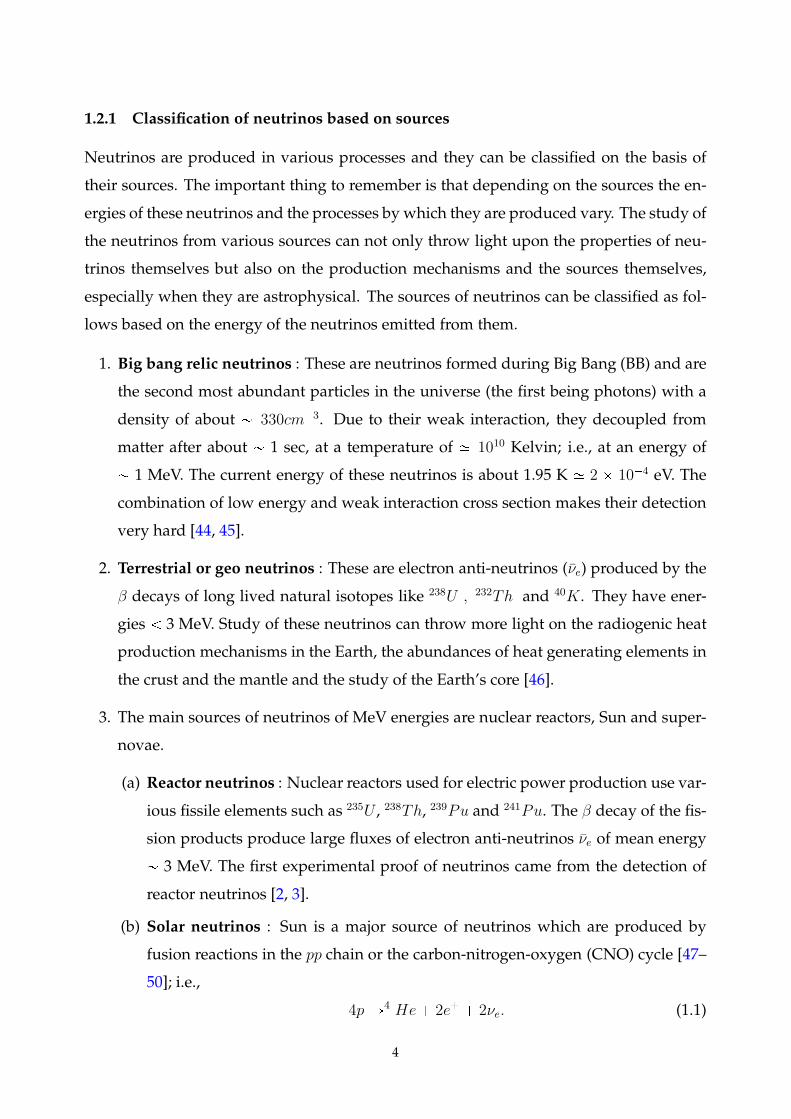
1.2.1 Classification of neutrinos based on sources

Neutrinos are produced in various processes and they can be classified on the basis of

their sources. The important thing to remember is that depending on the sources the en-

ergies of these neutrinos and the processes by which they are produced vary. The study of

the neutrinos from various sources can not only throw light upon the properties of neu-

trinos themselves but also on the production mechanisms and the sources themselves,

especially when they are astrophysical. The sources of neutrinos can be classified as fol-

lows based on the energy of the neutrinos emitted from them.

1. Big bang relic neutrinos : These are neutrinos formed during Big Bang (BB) and are

the second most abundant particles in the universe (the first being photons) with a

density of about 330cm3. Due to their weak interaction, they decoupled from

matter after about 1 sec, at a temperature of 1010 Kelvin; i.e., at an energy of

1 MeV. The current energy of these neutrinos is about 1.95 K 2 104 eV. The

combination of low energy and weak interaction cross section makes their detection

very hard [44, 45].

2. Terrestrial or geo neutrinos : These are electron anti-neutrinos (νe) produced by the

β decays of long lived natural isotopes like 238U , 232Th and 40K. They have ener-

gies 3 MeV. Study of these neutrinos can throw more light on the radiogenic heat

production mechanisms in the Earth, the abundances of heat generating elements in

the crust and the mantle and the study of the Earth’s core [46].

3. The main sources of neutrinos of MeV energies are nuclear reactors, Sun and super-

novae.

(a) Reactor neutrinos : Nuclear reactors used for electric power production use var-

ious fissile elements such as 235U , 238Th, 239Pu and 241Pu. The β decay of the fis-

sion products produce large fluxes of electron anti-neutrinos νe of mean energy

3 MeV. The first experimental proof of neutrinos came from the detection of

reactor neutrinos [2, 3].

(b) Solar neutrinos : Sun is a major source of neutrinos which are produced by

fusion reactions in the pp chain or the carbon-nitrogen-oxygen (CNO) cycle [47–

50]; i.e.,

4pÑ4 He 2e 2νe. (1.1)

4

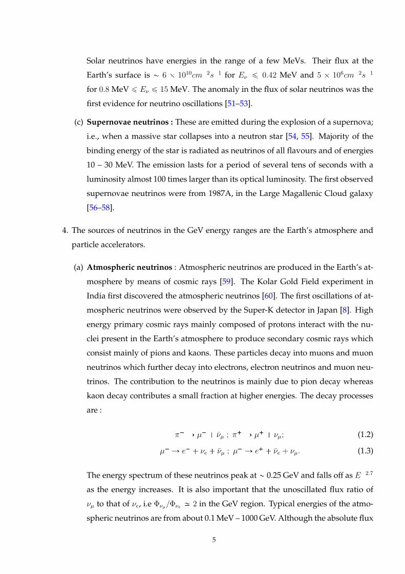
Solar neutrinos have energies in the range of a few MeVs. Their flux at the

Earth’s surface is 6 1010cm2s1 for Eν ¤ 0.42 MeV and 5 106cm2s1

for 0.8 MeV ¤ Eν ¤ 15 MeV. The anomaly in the flux of solar neutrinos was the

first evidence for neutrino oscillations [51–53].

(c) Supernovae neutrinos : These are emitted during the explosion of a supernova;

i.e., when a massive star collapses into a neutron star [54, 55]. Majority of the

binding energy of the star is radiated as neutrinos of all flavours and of energies

10 – 30 MeV. The emission lasts for a period of several tens of seconds with a

luminosity almost 100 times larger than its optical luminosity. The first observed

supernovae neutrinos were from 1987A, in the Large Magallenic Cloud galaxy

[56–58].

4. The sources of neutrinos in the GeV energy ranges are the Earth’s atmosphere and

particle accelerators.

(a) Atmospheric neutrinos : Atmospheric neutrinos are produced in the Earth’s at-

mosphere by means of cosmic rays [59]. The Kolar Gold Field experiment in

India first discovered the atmospheric neutrinos [60]. The first oscillations of at-

mospheric neutrinos were observed by the Super-K detector in Japan [8]. High

energy primary cosmic rays mainly composed of protons interact with the nu-

clei present in the Earth’s atmosphere to produce secondary cosmic rays which

consist mainly of pions and kaons. These particles decay into muons and muon

neutrinos which further decay into electrons, electron neutrinos and muon neu-

trinos. The contribution to the neutrinos is mainly due to pion decay whereas

kaon decay contributes a small fraction at higher energies. The decay processes

are :

π Ñ µ νµ ; π Ñ µ νµ; (1.2)

µ Ñ e νe νµ ; µ Ñ e νe νµ. (1.3)

The energy spectrum of these neutrinos peak at 0.25 GeV and falls off as E2.7

as the energy increases. It is also important that the unoscillated flux ratio of

νµ to that of νe, i.e ΦνµΦνe 2 in the GeV region. Typical energies of the atmo-

spheric neutrinos are from about 0.1MeV – 1000 GeV. Although the absolute flux

5

of atmospheric neutrinos is about 1 cm2s1 and the interaction cross sections

only 1038 cm2, it is worthwhile studying them, because of the wide range of

energies and distances offered by them over which neutrino oscillations can be

probed.

(b) Accelerator neutrinos : These are νµ or νµ of GeV ranges produced in particle

accelerators where protons are accelerated, hit on a target which produces pions

and kaons, which decay in flight inside a magnetic horn to give neutrinos. These

magnetic horns help to focus the parent pion or kaon, thus indirectly causing

the neutrinos to be emitted in a specific direction as a “beam” and also to selec-

tively produce neutrino or anti-neutrino beams by choosing the parent particle

accordingly. The advantage of using accelerator neutrinos is that a large flux

of neutrinos can be obtained as compared to the atmospheric neutrinos, even

though the oscillation parameters probed in both types of experiments are the

same. It should be noted that even though accelerators give a large flux of neu-

trinos, probes over a wide range of energies and distances are not possible with

them, thus making it necessary to tune the detectors precisely.

5. Galactic and extra galactic neutrinos : These are neutrinos which are produced as

secondary products in the interactions of charged cosmic rays accelerated in shock

processes inside the sources such as active galactic nuclei or gamma ray bursts. The

decay of the charged pions produced in these hadronic interactions give rise to these

ultra high energy neutrinos which travel without getting bent in the galactic mag-

netic field and hence carry information about the sources. The energy range of these

neutrinos are of the order of TeVs and PeVs [61–63].

1.3 Neutrino oscillation physics

According to the Standard Model (SM) of Particle Physics, there are three flavours of neu-

trinos, namely νe, νµ, ντ (and their anti-particles νe, νµ, ντ ) associated with each charged

lepton in the lepton doublet. They are neutral particles, owing to which they experience

only weak interactions [64]. In the Standard Model they are assumed to be massless. The

detection of neutrinos from several sources like the Sun and the atmosphere showed that

the flavour fluxes of neutrinos were not the same as predicted by theory. The only expla-

6

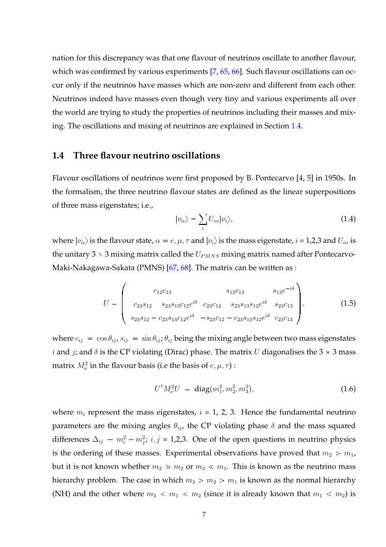
nation for this discrepancy was that one flavour of neutrinos oscillate to another flavour,

which was confirmed by various experiments [7, 65, 66]. Such flavour oscillations can oc-

cur only if the neutrinos have masses which are non-zero and different from each other.

Neutrinos indeed have masses even though very tiny and various experiments all over

the world are trying to study the properties of neutrinos including their masses and mix-

ing. The oscillations and mixing of neutrinos are explained in Section 1.4.

1.4 Three flavour neutrino oscillations

Flavour oscillations of neutrinos were first proposed by B. Pontecarvo [4, 5] in 1950s. In

the formalism, the three neutrino flavour states are defined as the linear superpositions

of three mass eigenstates; i.e.,

|ναy ¸

i

Uαi|νiy, (1.4)

where |ναy is the flavour state, α e, µ, τ and |νiy is the mass eigenstate, i = 1,2,3 and Uαi is

the unitary 3 3 mixing matrix called the UPMNS mixing matrix named after Pontecarvo-

Maki-Nakagawa-Sakata (PMNS) [67, 68]. The matrix can be written as :

U

c12c13 s12c13 s13eiδ

c23s12 s23s13c12eiδ c23c12 s23s13s12e

iδ s23c13

s23s12 c23s13c12eiδ

s23c12 c23s13s12eiδ c23c13

Æ

Æ

Æ

, (1.5)

where cij cos θij , sij sin θij ; θij being the mixing angle between twomass eigenstates

i and j; and δ is the CP violating (Dirac) phase. The matrix U diagonalises the 3 3 mass

matrixM2ν in the flavour basis (i.e the basis of e, µ, τ ) :

U :M2

νU diagpm2

1, m2

2, m2

3q, (1.6)

where mi represent the mass eigenstates, i = 1, 2, 3. Hence the fundamental neutrino

parameters are the mixing angles θij , the CP violating phase δ and the mass squared

differences ∆ij m2i m2

j ; i, j = 1,2,3. One of the open questions in neutrino physics

is the ordering of these masses. Experimental observations have proved that m2 ¡ m1,

but it is not known whether m3 " m2 or m3 ! m1. This is known as the neutrino mass

hierarchy problem. The case in which m3 ¡ m2 ¡ m1 is known as the normal hierarchy

(NH) and the other where m3 m1 m2 (since it is already known that m1 m2) is

7

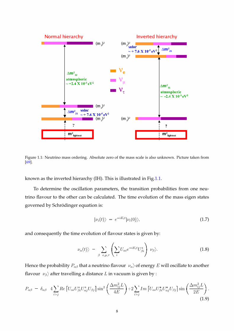
Figure 1.1: Neutrino mass ordering. Absolute zero of the mass scale is also unknown. Picture taken from[69].

known as the inverted hierarchy (IH). This is illustrated in Fig.1.1.

To determine the oscillation parameters, the transition probabilities from one neu-

trino flavour to the other can be calculated. The time evolution of the mass eigen states

governed by Schrodinger equation is:

|νiptqy eiEit|νip0qy, (1.7)

and consequently the time evolution of flavour states is given by:

|ναptqy ¸

βe,µ,τ

¸

i

UαieiEitU

βi

|νβy. (1.8)

Hence the probability Pαβ that a neutrino flavour |ναy of energy E will oscillate to another

flavour |νβy after travelling a distance L in vacuum is given by :

Pαβ δαβ4¸

i¡j

Re

UαiU

βiU

αjUβj

sin2

∆m2ijL

4E

2¸

i¡j

Im

UαiU

βiU

αjUβj

sin

∆m2ijL

2E

.

(1.9)

8

Similarly the probability Pαβ of an anti-neutrino flavour |ναy oscillating to a flavour |νβy

in vacuum is :

Pαβ δαβ4¸

i¡j

Re

UαiU

βiU

αjUβj

sin2

∆m2ijL

4E

2¸

i¡j

Im

UαiU

βiU

αjUβj

sin

∆m2ijL

2E

.

(1.10)

The probability is called “transition probability” when α β and “survival probability”

when α β. The oscillation length Loscij is defined such that the phase generated by ∆m2ij

becomes 2π; i.e.,

Loscij

4πE

∆m2ij

2.47ErMeV s

∆m2ijreV

2s

m 2.47ErGeV s

∆m2ijreV

2s

km. (1.11)

This quantity is used to design a neutrino experiment such that it is maximally sensitive

to the parameter to be probed. Thus the energy and distance of the neutrinos required to

obtain a certain level of sensitivity can be found out from Eq. 1.11.

1.4.1 Matter effects

Matter effects can alter the transition probabilities when neutrinos propagate through

matter. Probing matter effects can help in determining the ordering of the neutrino mass

eigenstates (whether it is NH or IH). The transition probabilities get modified when the

neutrinos (anti-neutrinos) propagate through matter. The time evolution of neutrinos in

the presence of matter is given by the expression :

id

dtrναs

1

2E

UM2U :

A

rναs, (1.12)

where rναs is the flavour eigenstate vector and

rναs

|νey

|νµy

|ντy

Æ

Æ

Æ

, M2

0 0 0

0 ∆m221

0

0 0 ∆m231

Æ

Æ

Æ

, A

ACC 0 0

0 0 0

0 0 0

Æ

Æ

Æ

.

The matter term (ignoring the diagonal neutral current contribution) is given by

ACC 2?

2GFneE 7.63 105eV2 ρ(gm/cc) E(GeV), (1.13)

where, GF is the Fermi constant and ne is the electron number density in matter and ρ

is the matter density. For anti-neutrinos the sign of ACC and the phase δ in Eq. 1.12 get

9

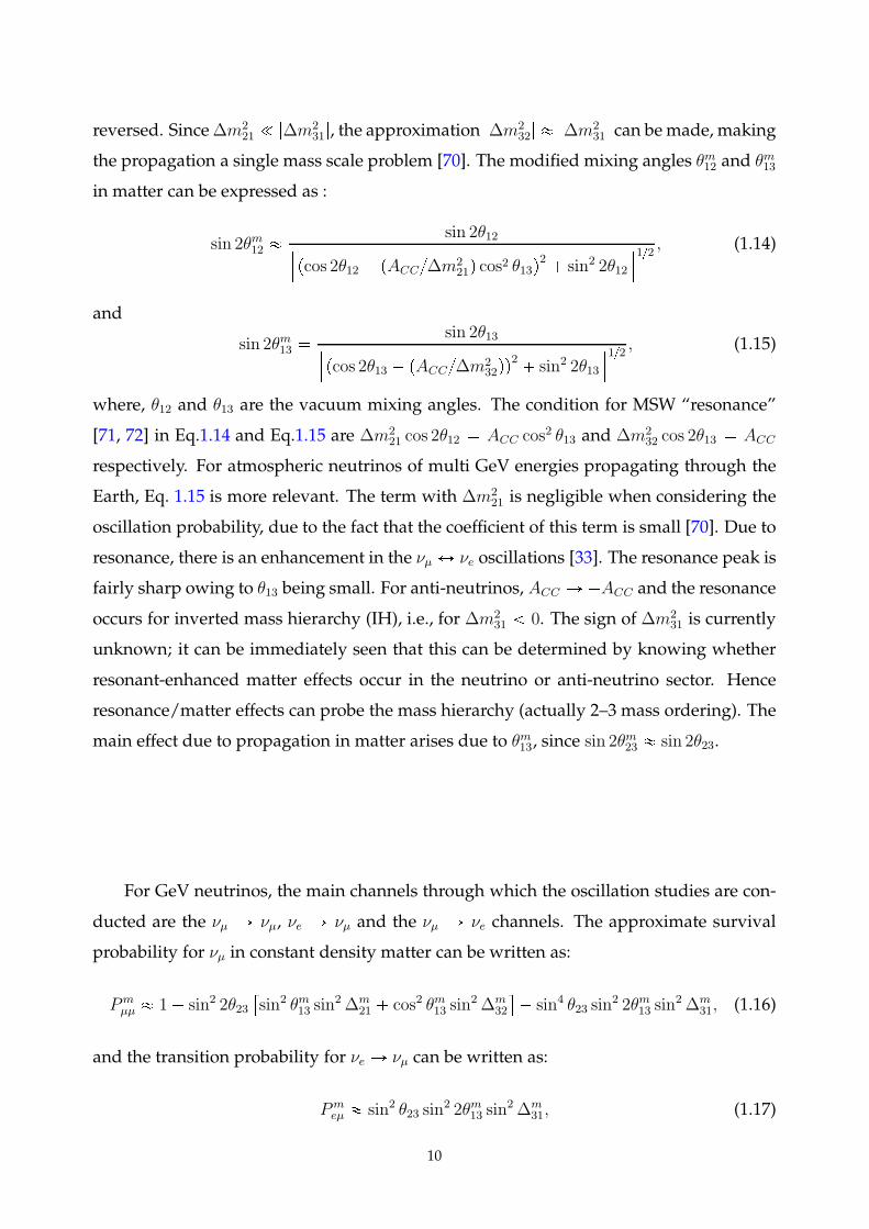
reversed. Since∆m221 ! |∆m2

31|, the approximation |∆m232| |∆m2

31| can bemade, making

the propagation a single mass scale problem [70]. The modified mixing angles θm12 and θm13

in matter can be expressed as :

sin 2θm12

sin 2θ12

pcos 2θ12 pACC∆m221q cos2 θ13q

2 sin2 2θ12

12, (1.14)

and

sin 2θm13 sin 2θ13

pcos 2θ13 pACC∆m232qq

2 sin2 2θ13

12, (1.15)

where, θ12 and θ13 are the vacuum mixing angles. The condition for MSW “resonance”

[71, 72] in Eq.1.14 and Eq.1.15 are ∆m221 cos 2θ12 ACC cos2 θ13 and ∆m2

32 cos 2θ13 ACC

respectively. For atmospheric neutrinos of multi GeV energies propagating through the

Earth, Eq. 1.15 is more relevant. The term with ∆m221

is negligible when considering the

oscillation probability, due to the fact that the coefficient of this term is small [70]. Due to

resonance, there is an enhancement in the νµ Ø νe oscillations [33]. The resonance peak is

fairly sharp owing to θ13 being small. For anti-neutrinos, ACC Ñ ACC and the resonance

occurs for inverted mass hierarchy (IH), i.e., for ∆m231 0. The sign of ∆m2

31 is currently

unknown; it can be immediately seen that this can be determined by knowing whether

resonant-enhanced matter effects occur in the neutrino or anti-neutrino sector. Hence

resonance/matter effects can probe the mass hierarchy (actually 2–3 mass ordering). The

main effect due to propagation in matter arises due to θm13, since sin 2θm

23 sin 2θ23.

For GeV neutrinos, the main channels through which the oscillation studies are con-

ducted are the νµ Ñ νµ, νe Ñ νµ and the νµ Ñ νe channels. The approximate survival

probability for νµ in constant density matter can be written as:

Pmµµ 1 sin2 2θ23

sin2 θm13sin2∆m

21 cos2 θm

13sin2∆m

32

sin4 θ23 sin2 2θm

13sin2∆m

31, (1.16)

and the transition probability for νe Ñ νµ can be written as:

Pmeµ sin2 θ23 sin

2 2θm13 sin2∆m

31, (1.17)

10

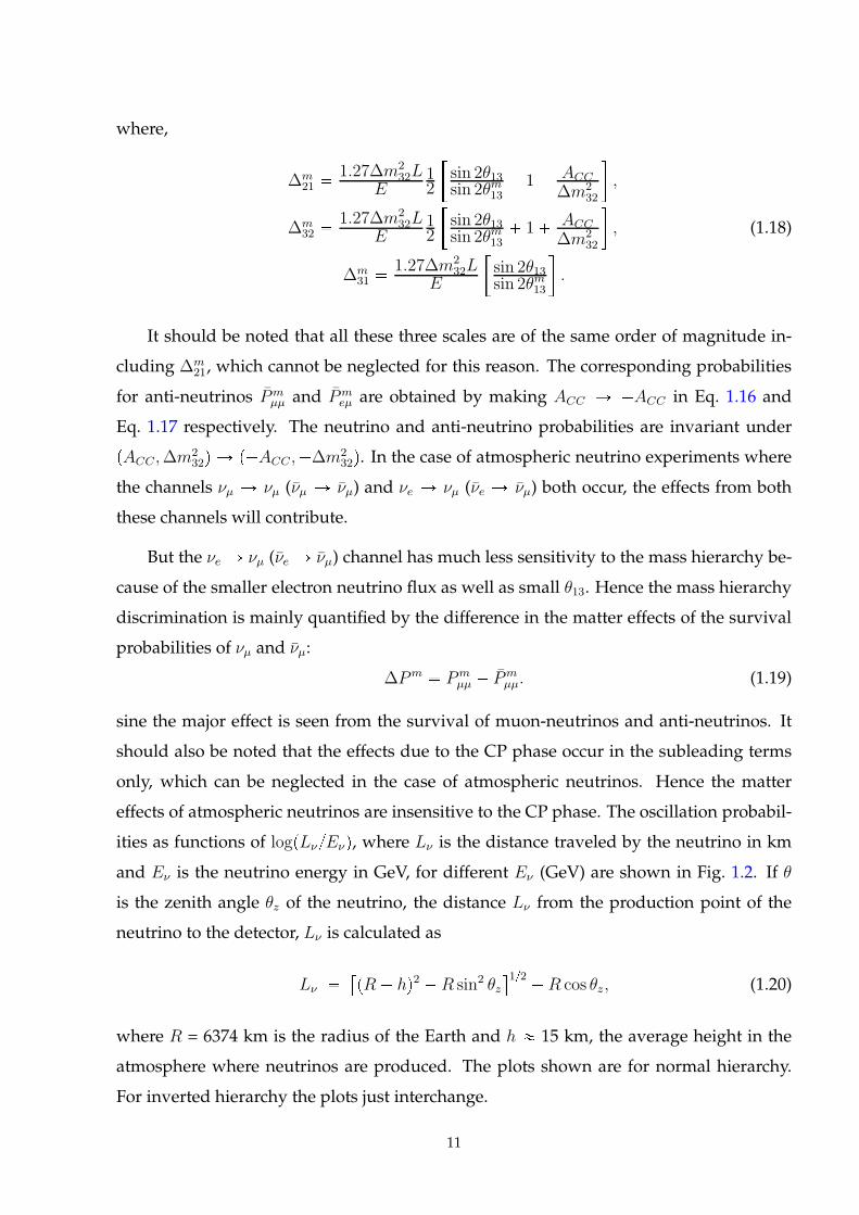
where,

∆m21

1.27∆m2

32L

E12

sin 2θ13sin 2θm

13

1 ACC∆m2

32

,

∆m32

1.27∆m2

32L

E12

sin 2θ13sin 2θm13

1 ACC∆m2

32

, (1.18)

∆m31

1.27∆m2

32LE

sin 2θ13sin 2θm13

.

It should be noted that all these three scales are of the same order of magnitude in-

cluding ∆m21, which cannot be neglected for this reason. The corresponding probabilities

for anti-neutrinos Pmµµ and Pm

eµ are obtained by making ACC Ñ ACC in Eq. 1.16 and

Eq. 1.17 respectively. The neutrino and anti-neutrino probabilities are invariant under

pACC ,∆m232q Ñ pACC ,∆m

232q. In the case of atmospheric neutrino experiments where

the channels νµ Ñ νµ (νµ Ñ νµ) and νe Ñ νµ (νe Ñ νµ) both occur, the effects from both

these channels will contribute.

But the νe Ñ νµ (νe Ñ νµ) channel has much less sensitivity to the mass hierarchy be-

cause of the smaller electron neutrino flux as well as small θ13. Hence the mass hierarchy

discrimination is mainly quantified by the difference in the matter effects of the survival

probabilities of νµ and νµ:

∆Pm Pm

µµ Pmµµ. (1.19)

sine the major effect is seen from the survival of muon-neutrinos and anti-neutrinos. It

should also be noted that the effects due to the CP phase occur in the subleading terms

only, which can be neglected in the case of atmospheric neutrinos. Hence the matter

effects of atmospheric neutrinos are insensitive to the CP phase. The oscillation probabil-

ities as functions of logpLνEνq, where Lν is the distance traveled by the neutrino in km

and Eν is the neutrino energy in GeV, for different Eν (GeV) are shown in Fig. 1.2. If θ

is the zenith angle θz of the neutrino, the distance Lν from the production point of the

neutrino to the detector, Lν is calculated as

Lν

pR hq2 R sin2 θz12

R cos θz, (1.20)

where R = 6374 km is the radius of the Earth and h 15 km, the average height in the

atmosphere where neutrinos are produced. The plots shown are for normal hierarchy.

For inverted hierarchy the plots just interchange.

11

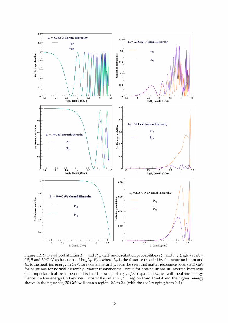
(GeV))ν (km)/Eν

log(L1.5 2 2.5 3 3.5 4 4.5

Osc

illa

tion

pro

ba

bili

ties

0

0.2

0.4

0.6

0.8

1

1.2

1.4

= 0.5 GeV; Normal HierarchyνE

µµP

µµP

(GeV))ν (km)/Eν

log(L1.5 2 2.5 3 3.5 4 4.5

Osc

illa

tion

pro

ba

bili

ties

0

0.05

0.1

0.15

0.2

0.25 = 0.5 GeV; Normal HierarchyνE

µeP

µeP

(GeV))ν (km)/Eν

log(L0.5 1 1.5 2 2.5 3 3.5

Osc

illa

tion

pro

ba

bili

ties

0

0.2

0.4

0.6

0.8

1


µµP

µµP

(GeV))ν (km)/Eν

log(L0.5 1 1.5 2 2.5 3 3.5

Osc

illa

tion

pro

ba

bili

ties

0

0.1

0.2

0.3

0.4

0.5


µeP

µeP

(GeV)ν (km)/EνL0 0.5 1 1.5 2 2.5

Osc

illa

tion

pro

ba

bili

ties

0.2

0.4

0.6

0.8

1


µµP

µµP

(GeV)ν (km)/EνL0 0.5 1 1.5 2 2.5

Osc

illa

tion

pro

ba

bili

ties

0

0.002

0.004

0.006

0.008


µeP

µeP

Figure 1.2: Survival probabilities Pµµ and Pµµ (left) and oscillation probabilities Peµ and Peµ (right) at Eν =0.5, 5 and 30 GeV as functions of logpLνEνq, where Lν is the distance traveled by the neutrino in km andEν is the neutrino energy in GeV, for normal hierarchy. It can be seen that matter resonance occurs at 5 GeVfor neutrinos for normal hierarchy. Matter resonance will occur for anti-neutrinos in inverted hierarchy.One important feature to be noted is that the range of logpLνEνq spanned varies with neutrino energy.Hence the low energy 0.5 GeV neutrinos will span an LνEν region from 1.5–4.4 and the highest energyshown in the figure viz, 30 GeV will span a region -0.3 to 2.6 (with the cos θ ranging from 0–1).

12

The matter effects are more prominent for neutrinos in normal hierarchy and for anti-

neutrinos with inverted hierarchy. Resonance occurs for neutrinos in normal hierarchy

and for anti-neutrinos in inverted hierarchy. This is because the matter effects are en-

hanced when both ACC and ∆m232 have the same sign and are depleted when they have

opposite signs as can be seen from Eqs. 1.16,1.17 and 1.19. This enables neutrino mass

hierarchy distinction by studying the Earth matter effects.

Thus it can be seen that in the 3-flavour oscillation scenario the transition proba-

bilities, both of neutrinos and anti-neutrinos, depend on all the oscillation parameters

namely θ12, θ13, θ23, ∆m221, ∆m

232 and the CP phase δ. Hence the precise measurement of

the magnitude of all these quantities and determining the sign of the mass squared differ-

ences are very important. Several neutrino detectors, spanning over different baselines

and energies are running and many more are being planned all over the world, including

the INO, for this purpose. The next section lists some of the most important neutrino

oscillation experiments. The list contains experiments which have finished taking data as

well as currently running ones.

1.5 Some important neutrino oscillation experiments

Neutrino physics is an experiment driven field. Starting from the first detection of neu-

trinos which proved Pauli’s theory to be right [2, 3] through the solar neutrino puzzle

and its resolution, [73] to the recent measurement of θ13 [11], experiments have played a

major role in formulating and improving our understanding of neutrinos. Some of the

important neutrino oscillation experiments are listed in this section. The design of each

experiment is optimally done specific to the sensitivity to the parameter to be measured.

1. Homestake experiment [51, 73–75]: This was a radiochemical experiment designed

to detect and measure the electron neutrino (νe) flux from the sun. Only one third

of the predicted flux [47] was detected in the experiment. This discrepancy with the

theory led to the famous “solar neutrino problem” which was the first indication of

flavour oscillations among neutrinos as well as non-zero neutrino masses.

2. Sudbury Neutrino Observatory (SNO)[7, 76, 77] : This was the solar neutrino ex-

periment which used 2 ktons of heavy water to confirm solar neutrino oscillations

by detecting solar neutrinos through both charged current and neutral current inter-

13

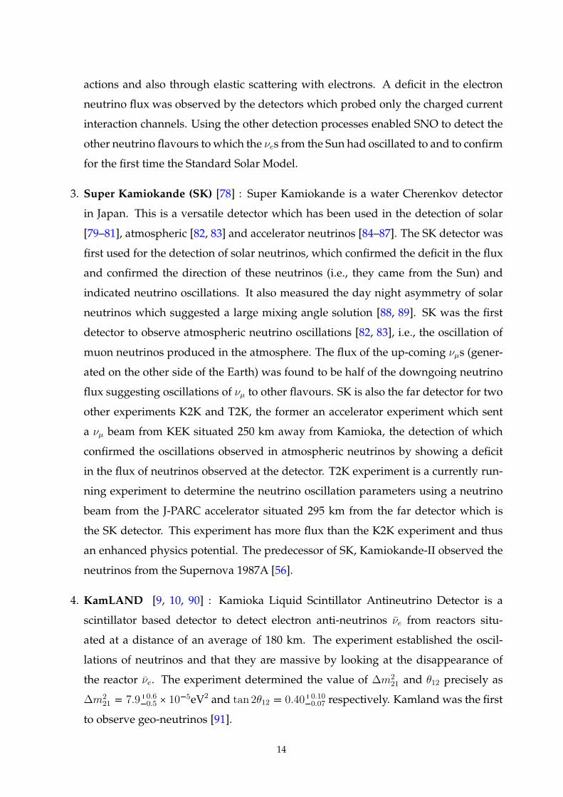
actions and also through elastic scattering with electrons. A deficit in the electron

neutrino flux was observed by the detectors which probed only the charged current

interaction channels. Using the other detection processes enabled SNO to detect the

other neutrino flavours to which the νes from the Sun had oscillated to and to confirm

for the first time the Standard Solar Model.

3. Super Kamiokande (SK) [78] : Super Kamiokande is a water Cherenkov detector

in Japan. This is a versatile detector which has been used in the detection of solar

[79–81], atmospheric [82, 83] and accelerator neutrinos [84–87]. The SK detector was

first used for the detection of solar neutrinos, which confirmed the deficit in the flux

and confirmed the direction of these neutrinos (i.e., they came from the Sun) and

indicated neutrino oscillations. It also measured the day night asymmetry of solar

neutrinos which suggested a large mixing angle solution [88, 89]. SK was the first

detector to observe atmospheric neutrino oscillations [82, 83], i.e., the oscillation of

muon neutrinos produced in the atmosphere. The flux of the up-coming νµs (gener-

ated on the other side of the Earth) was found to be half of the downgoing neutrino

flux suggesting oscillations of νµ to other flavours. SK is also the far detector for two

other experiments K2K and T2K, the former an accelerator experiment which sent

a νµ beam from KEK situated 250 km away from Kamioka, the detection of which

confirmed the oscillations observed in atmospheric neutrinos by showing a deficit

in the flux of neutrinos observed at the detector. T2K experiment is a currently run-

ning experiment to determine the neutrino oscillation parameters using a neutrino

beam from the J-PARC accelerator situated 295 km from the far detector which is

the SK detector. This experiment has more flux than the K2K experiment and thus

an enhanced physics potential. The predecessor of SK, Kamiokande-II observed the

neutrinos from the Supernova 1987A [56].

4. KamLAND [9, 10, 90] : Kamioka Liquid Scintillator Antineutrino Detector is a

scintillator based detector to detect electron anti-neutrinos νe from reactors situ-

ated at a distance of an average of 180 km. The experiment established the oscil-

lations of neutrinos and that they are massive by looking at the disappearance of

the reactor νe. The experiment determined the value of ∆m221

and θ12 precisely as

∆m221 7.90.6

0.5105eV2 and tan 2θ12 0.400.100.07 respectively. Kamland was the first

to observe geo-neutrinos [91].

14

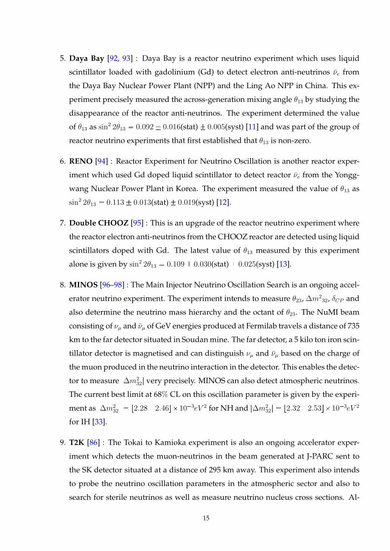
5. Daya Bay [92, 93] : Daya Bay is a reactor neutrino experiment which uses liquid

scintillator loaded with gadolinium (Gd) to detect electron anti-neutrinos νe from

the Daya Bay Nuclear Power Plant (NPP) and the Ling Ao NPP in China. This ex-

periment precisely measured the across-generation mixing angle θ13 by studying the

disappearance of the reactor anti-neutrinos. The experiment determined the value

of θ13 as sin2 2θ13 0.092 0.016(stat) 0.005(syst) [11] and was part of the group of

reactor neutrino experiments that first established that θ13 is non-zero.

6. RENO [94] : Reactor Experiment for Neutrino Oscillation is another reactor exper-

iment which used Gd doped liquid scintillator to detect reactor νe from the Yongg-

wang Nuclear Power Plant in Korea. The experiment measured the value of θ13 as

sin2 2θ13 0.113 0.013(stat) 0.019(syst) [12].

7. Double CHOOZ [95] : This is an upgrade of the reactor neutrino experiment where

the reactor electron anti-neutrinos from the CHOOZ reactor are detected using liquid

scintillators doped with Gd. The latest value of θ13 measured by this experiment

alone is given by sin2 2θ13 0.109 0.030(stat) 0.025(syst) [13].

8. MINOS [96–98] : The Main Injector Neutrino Oscillation Search is an ongoing accel-

erator neutrino experiment. The experiment intends to measure θ23, ∆m232, δCP and

also determine the neutrino mass hierarchy and the octant of θ23. The NuMI beam

consisting of νµ and νµ of GeV energies produced at Fermilab travels a distance of 735

km to the far detector situated in Soudanmine. The far detector, a 5 kilo ton iron scin-

tillator detector is magnetised and can distinguish νµ and νµ based on the charge of

themuon produced in the neutrino interaction in the detector. This enables the detec-

tor to measure |∆m232| very precisely. MINOS can also detect atmospheric neutrinos.

The current best limit at 68% CL on this oscillation parameter is given by the experi-

ment as |∆m232| r2.282.46s103eV 2 for NH and |∆m2

32| r2.322.53s103eV 2

for IH [33].

9. T2K [86] : The Tokai to Kamioka experiment is also an ongoing accelerator exper-

iment which detects the muon-neutrinos in the beam generated at J-PARC sent to

the SK detector situated at a distance of 295 km away. This experiment also intends

to probe the neutrino oscillation parameters in the atmospheric sector and also to

search for sterile neutrinos as well as measure neutrino nucleus cross sections. Al-

15

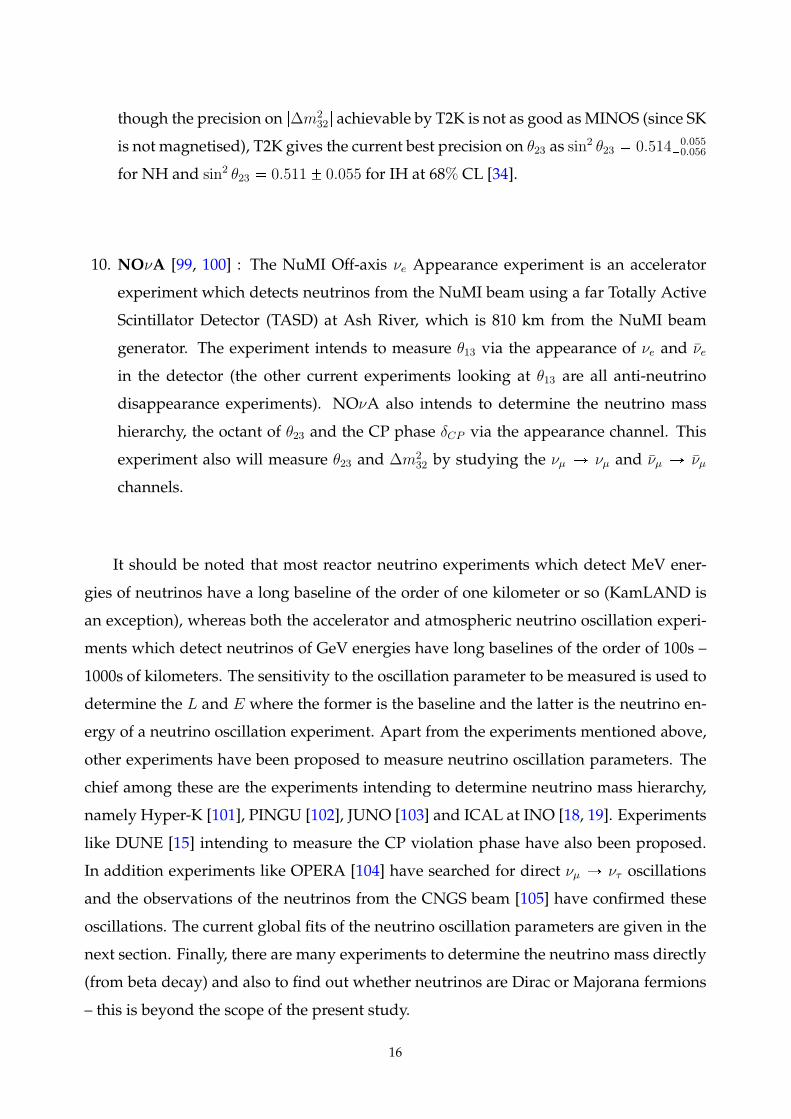
though the precision on |∆m232| achievable by T2K is not as good asMINOS (since SK

is not magnetised), T2K gives the current best precision on θ23 as sin2 θ23 0.5140.055

0.056

for NH and sin2 θ23 0.511 0.055 for IH at 68% CL [34].

10. NOνA [99, 100] : The NuMI Off-axis νe Appearance experiment is an accelerator

experiment which detects neutrinos from the NuMI beam using a far Totally Active

Scintillator Detector (TASD) at Ash River, which is 810 km from the NuMI beam

generator. The experiment intends to measure θ13 via the appearance of νe and νe

in the detector (the other current experiments looking at θ13 are all anti-neutrino

disappearance experiments). NOνA also intends to determine the neutrino mass

hierarchy, the octant of θ23 and the CP phase δCP via the appearance channel. This

experiment also will measure θ23 and ∆m232

by studying the νµ Ñ νµ and νµ Ñ νµ

channels.

It should be noted that most reactor neutrino experiments which detect MeV ener-

gies of neutrinos have a long baseline of the order of one kilometer or so (KamLAND is

an exception), whereas both the accelerator and atmospheric neutrino oscillation experi-

ments which detect neutrinos of GeV energies have long baselines of the order of 100s –

1000s of kilometers. The sensitivity to the oscillation parameter to be measured is used to

determine the L and E where the former is the baseline and the latter is the neutrino en-

ergy of a neutrino oscillation experiment. Apart from the experiments mentioned above,

other experiments have been proposed to measure neutrino oscillation parameters. The

chief among these are the experiments intending to determine neutrino mass hierarchy,

namely Hyper-K [101], PINGU [102], JUNO [103] and ICAL at INO [18, 19]. Experiments

like DUNE [15] intending to measure the CP violation phase have also been proposed.

In addition experiments like OPERA [104] have searched for direct νµ Ñ ντ oscillations

and the observations of the neutrinos from the CNGS beam [105] have confirmed these

oscillations. The current global fits of the neutrino oscillation parameters are given in the

next section. Finally, there are many experiments to determine the neutrino mass directly

(from beta decay) and also to find out whether neutrinos are Dirac or Majorana fermions

– this is beyond the scope of the present study.

16

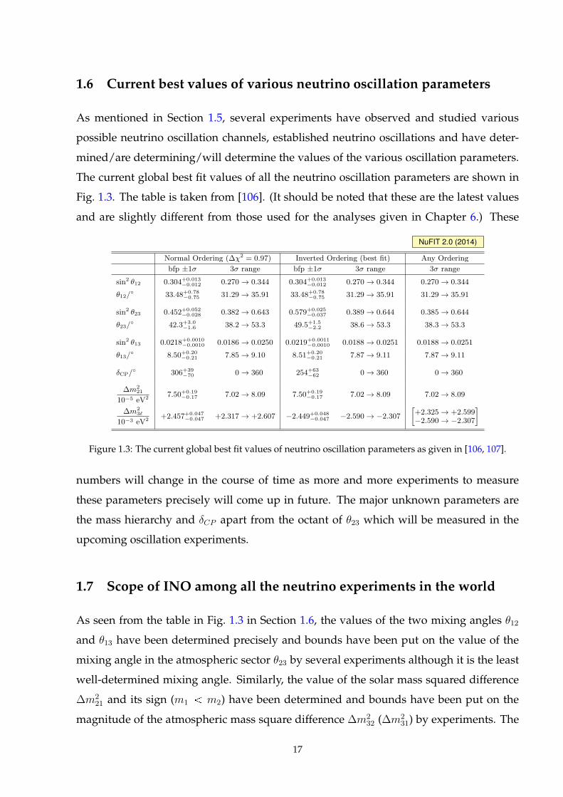
1.6 Current best values of various neutrino oscillation parameters

As mentioned in Section 1.5, several experiments have observed and studied various

possible neutrino oscillation channels, established neutrino oscillations and have deter-

mined/are determining/will determine the values of the various oscillation parameters.

The current global best fit values of all the neutrino oscillation parameters are shown in

Fig. 1.3. The table is taken from [106]. (It should be noted that these are the latest values

and are slightly different from those used for the analyses given in Chapter 6.) These

NuFIT 2.0 (2014)

Normal Ordering (∆χ2 = 0.97) Inverted Ordering (best fit) Any Ordering

bfp ±1σ 3σ range bfp ±1σ 3σ range 3σ range

sin2 θ12 0.304+0.013−0.012 0.270 → 0.344 0.304+0.013

−0.012 0.270 → 0.344 0.270 → 0.344

θ12/ 33.48+0.78

−0.75 31.29 → 35.91 33.48+0.78−0.75 31.29 → 35.91 31.29 → 35.91

sin2 θ23 0.452+0.052−0.028 0.382 → 0.643 0.579+0.025

−0.037 0.389 → 0.644 0.385 → 0.644

θ23/ 42.3+3.0

−1.6 38.2 → 53.3 49.5+1.5−2.2 38.6 → 53.3 38.3 → 53.3

sin2 θ13 0.0218+0.0010−0.0010 0.0186 → 0.0250 0.0219+0.0011

−0.0010 0.0188 → 0.0251 0.0188 → 0.0251

θ13/ 8.50+0.20

−0.21 7.85 → 9.10 8.51+0.20−0.21 7.87 → 9.11 7.87 → 9.11

δCP/ 306+39

−70 0 → 360 254+63−62 0 → 360 0 → 360

∆m221

10−5 eV27.50+0.19

−0.17 7.02 → 8.09 7.50+0.19−0.17 7.02 → 8.09 7.02 → 8.09

∆m23ℓ

10−3 eV2+2.457+0.047

−0.047 +2.317 → +2.607 −2.449+0.048−0.047 −2.590 → −2.307

[

+2.325 → +2.599−2.590 → −2.307

]

Figure 1.3: The current global best fit values of neutrino oscillation parameters as given in [106, 107].

numbers will change in the course of time as more and more experiments to measure

these parameters precisely will come up in future. The major unknown parameters are

the mass hierarchy and δCP apart from the octant of θ23 which will be measured in the

upcoming oscillation experiments.

1.7 Scope of INO among all the neutrino experiments in the world

As seen from the table in Fig. 1.3 in Section 1.6, the values of the two mixing angles θ12

and θ13 have been determined precisely and bounds have been put on the value of the

mixing angle in the atmospheric sector θ23 by several experiments although it is the least

well-determined mixing angle. Similarly, the value of the solar mass squared difference

∆m221

and its sign (m1 m2) have been determined and bounds have been put on the

magnitude of the atmospheric mass square difference ∆m232 (∆m

231) by experiments. The

17

most important open question in neutrino physics as of today is the sign of∆m232 (∆m

231),

which will determine whether the neutrino masses are ordered in the normal fashion

(m1 m2 m3) or the inverted fashion (m3 m1 m2). Other important questions

are about the octant of θ23 and CP violation which are also being probed by many exper-

iments. Since several experiments are sensitive to different channels and the property of

the detector actually determines to what extent the experiment can be sensitive to neu-

trino oscillation parameters, it is important to design detectors which can answer specific

questions. It is in such a context that the Iron Calorimeter (ICAL) detector at the proposed

India-based Neutrino Observatory becomes important.

The proposed ICAL detector is a 50 kilo ton magnetisable detector which will be

mainly sensitive to atmospheric muon neutrinos and anti-neutrinos. This detector, ow-

ing to its magnetisability, can distinguish between µ and µ produced in the final state

of a charged-current neutrino interaction with iron. Thus by looking at the charge of the

muon, it can precisely tag an event as a neutrino or anti-neutrino event, which an unmag-

netisable water Cherenkov detector cannot do. This inturn makes it ideal for the detection

of neutrino and anti-neutrino events, separately, and thus determine the mass hierarchy

of neutrinos by studying the Earth matter effects discussed in Section 1.4.1. The source

of neutrinos in ICAL being atmospheric neutrinos opens up a new prospect of probing a

wide range of distancesL and energiesE overwhich the oscillations can be studied. ICAL

will be a huge detector, hence with reasonable exposure, there will be enough number of

events with which the studies can be done. Not only can ICAL determine the neutrino

mass hierarchy, but it can perform precision measurements of θ23 and ∆m232, which will

further contribute to the global fits to these parameters. As of now ICAL is one of the ex-

periments, despite being simple in design and working, that can do amazing physics and

will definitely have an impact on the neutrino parameter values. It is also noteworthy

that the ICAL can not only do neutrino oscillation studies, but also dark matter studies,

searches for magnetic monopoles and even sterile neutrino searches [19].

1.8 Scope of this thesis

This thesis reports the detailed simulation studies of the ICAL detector and its physics

potential, with emphasis on the hadrons produced in the neutrino interactions in the de-

tector. Although ICAL detector is optimised for the detection andmeasurement of muons

18

and their momenta, the hadrons produced in the charged current interactions which pro-

duce these muons also carry much information which will enhance the sensitivity of the

ICAL to oscillation parameters. Thus it is necessary to characterise the response of the

detector to hadrons, their energy and direction have to be determined as precisely as pos-

sible. The description of the ICAL detector geometry and its various components along

with the different interactions which can be detected are given in Chapter 2. A detailed

report of the simulation studies of the energy resolution of hadrons in ICAL is presented

in Chapter 3. The simulation studies on the reconstruction of hadron shower direction

in ICAL are discussed in Chapter 4. The muon momentum resolution and charge identi-

fication capability of the ICAL have been studied elsewhere and are briefly presented in

Chapter 5 for completeness. Since the charged-current interactions of muon neutrinos are

of main interest in ICAL, the techniques to identify these events from other events such

as the charged current electron neutrino events and neutral current events are also dis-

cussed in Chapter 5. The muonmomentum and hadron energy resolutions obtained from

the simulation studies are compiled as look-up tables and used in the oscillation analysis

described in Chapter 6. A detailed simulation study on the sensitivity of ICAL to neutrino

oscillation parameters in the extended energy range of 0.5–25 GeV of the observed muon

is presented in Chapter 6. This study is a refinement over the earlier work presented in

[27, 29, 30]. Two types of analyses, one which uses muon energy and direction informa-

tion only and the other which makes use of muon energy,direction and hadron energy,

are illustrated. Along with these, the effect of constraining the flux ratio of νµ and νµ is

also studied. The conclusions and outlook derived from the analyses performed in these

chapters along with the future scope are elucidated in Chapter 7.

19

2 ICAL @ INO

As mentioned in Chapter 1, one of the open questions in neutrino physics as of today is

the mass ordering of neutrinos. To resolve this puzzle, several experiments [18, 19, 99–

103] have been proposed and some are being built, all over the world. The experiment

proposed in India, namely the India-based Neutrino Observatory (INO) [18, 19] will

house a 50 kton magnetisable Iron Calorimeter detector (called ICAL) to detect atmo-

spheric neutrinos and study neutrino oscillation parameters by probing the Earth matter

effects of neutrinos as they propagate through various layers of the Earth. The detector

will be located in Bodi West Hills in Theni District of Tamil Nadu, India, in a cavern built

in the mountain such that there is a minimum rock cover of 1 km on all sides to re-

duce the cosmic ray background. The main physics goals of the ICAL detector involve

precision measurement of the oscillation parameters sin2 θ23 and |∆m232| where θ23 is the

mixing angle and the latter is the mass squared difference in the atmospheric sector. As

mentioned above, ICAL also can determine the sign of ∆m232, i.e., the neutrino mass hier-

archy. A brief description of the ICAL detector, to familiarise with the detector structure,

is given in the following sections. The major components of the detector are iron plates

which act as the passive detector with which the neutrinos interact and the active resis-

tive plate chambers (RPCs) which detect the charged particles produced in these neutrino

interactions.

2.1 Why a detector with iron and resistive plate chambers?

It is interesting to know why the combination of iron and RPCs has been chosen to build

the detector. Two of the major deciding factors in the design of any detector will be

the physics goals of the experiment and cost effectiveness. The iron-RPC combination is

optimal for the kind of physics ICAL intends to study. The main reasons why ICAL will

be built with iron are the following:

• The total number of unoscillated neutrino events in the detector can be expressed as

:

N Φ σ nd t, (2.1)

where Φ is the unoscillated flux of neutrinos, σ is the interaction cross section, nd

is the number of targets in the detector, t is the exposure time. In the case of at-

mospheric neutrinos, the fluxes cannot be controlled. Oscillations will further de-

crease the neutrino flux. Interaction cross section also cannot be controlled since it

is an intrinsic property of the particle. So with these constraints, to obtain a reason-

able number of events so as to do oscillation studies, either the number of targets

or the exposure time must be increased. To increase the number of targets, a large

mass/volume, say a megaton/km3 of a low density material like water (as in the

case of Ice Cube detector), can be used, or a smaller mass/volume say of the order

of kilo ton/m3 of a high density material like iron (high Z material) can be used.

The proposed ICAL detector consists of 50 kilo tons of iron as the target material;

iron being a high Z material makes the detector a compact one which can detect a

reasonable number of events in 5 or 10 years of exposure.

• The main physics studies in ICAL are the measurement of the neutrino oscillation

parameters, i.e., the precision measurement of the neutrino mixing angle θ23 and the

mass squared difference ∆m232. The sign of ∆m2

32i.e., neutrino mass hierarchy, can

be determined by probing the earth matter effect as the neutrinos pass through the

Earth. All these studies will mainly be done by the detection of charged current

muon neutrino events, in which a νµ or νµ interacts with the iron nucleus and pro-

duces a µ or µ accordingly. The iron in the detector now acts not only as the target

material, but also as a magnet which can be used to distinguish these µ and µ by

using the direction of bending of these particles in the magnetic field. Thus it enables

the identification of a particular type of charge which enhances the sensitivities of the

ICAL to oscillation parameters as opposed to detectors which cannot be magnetised

at all.

Determining the direction of the incoming neutrino is crucial in oscillation studies. To

determine if a neutrino is upcoming or down-going, time information is important and

the detector should have excellent timing resolution of the order of 1 ns. The resistive

plate chamber detectors (RPCs), which are gaseous detectors, have such a timing resolu-

22

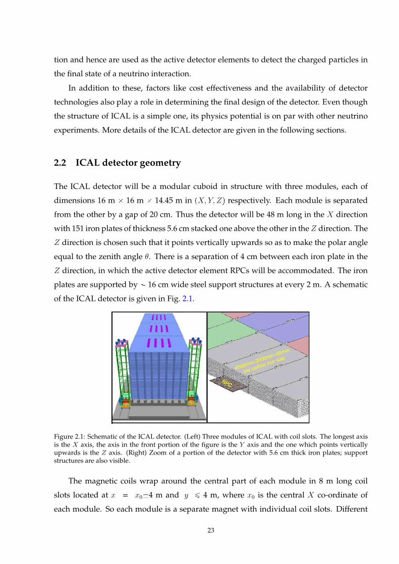
tion and hence are used as the active detector elements to detect the charged particles in

the final state of a neutrino interaction.

In addition to these, factors like cost effectiveness and the availability of detector

technologies also play a role in determining the final design of the detector. Even though

the structure of ICAL is a simple one, its physics potential is on par with other neutrino

experiments. More details of the ICAL detector are given in the following sections.

2.2 ICAL detector geometry

The ICAL detector will be a modular cuboid in structure with three modules, each of

dimensions 16 m 16 m 14.45 m in pX, Y, Zq respectively. Each module is separated

from the other by a gap of 20 cm. Thus the detector will be 48 m long in the X direction

with 151 iron plates of thickness 5.6 cm stacked one above the other in the Z direction. The

Z direction is chosen such that it points vertically upwards so as to make the polar angle

equal to the zenith angle θ. There is a separation of 4 cm between each iron plate in the

Z direction, in which the active detector element RPCs will be accommodated. The iron

plates are supported by 16 cm wide steel support structures at every 2 m. A schematic

of the ICAL detector is given in Fig. 2.1.

Figure 2.1: Schematic of the ICAL detector. (Left) Three modules of ICAL with coil slots. The longest axisis the X axis, the axis in the front portion of the figure is the Y axis and the one which points verticallyupwards is the Z axis. (Right) Zoom of a portion of the detector with 5.6 cm thick iron plates; supportstructures are also visible.

The magnetic coils wrap around the central part of each module in 8 m long coil

slots located at x x04 m and |y| ¤ 4 m, where x0 is the central X co-ordinate of

each module. So each module is a separate magnet with individual coil slots. Different

23

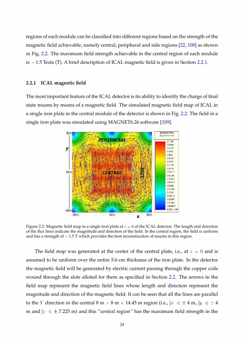
regions of each module can be classified into different regions based on the strength of the

magnetic field achievable, namely central, peripheral and side regions [22, 108] as shown

in Fig. 2.2. The maximum field strength achievable in the central region of each module

is 1.5 Tesla (T). A brief description of ICAL magnetic field is given in Section 2.2.1.

2.2.1 ICAL magnetic field

The most important feature of the ICAL detector is its ability to identify the charge of final

state muons by means of a magnetic field. The simulated magnetic field map of ICAL in

a single iron plate in the central module of the detector is shown in Fig. 2.2. The field in a

single iron plate was simulated using MAGNET6.26 software [109].

Figure 2.2: Magnetic field map in a single iron plate at z 0 of the ICAL detector. The length and directionof the flux lines indicate the magnitude and direction of the field. In the central region, the field is uniformand has a strength of 1.5 T which provides the best reconstruction of muons in this region.

The field map was generated at the center of the central plate, i.e., at z 0 and is

assumed to be uniform over the entire 5.6 cm thickness of the iron plate. In the detector

the magnetic field will be generated by electric current passing through the copper coils

wound through the slots alloted for them as specified in Section 2.2. The arrows in the

field map represent the magnetic field lines whose length and direction represent the

magnitude and direction of the magnetic field. It can be seen that all the lines are parallel

to the Y direction in the central 8 m 8 m 14.45 m region (i.e., |x| ¤ 4 m, |y| ¤ 4

m and |z| ¤ 7.225 m) and this “central region” has the maximum field strength in the

24

whole module. It should be noted that both the magnitude and direction of the magnetic

field are uniform in this region.

In the Y direction outside the central region, where |y| ¥ 4 m, both the magnitude

and direction of the magnetic field change maximally; the field strength falls to zero at

the corners of the module. This region is called the “peripheral region” of the detector.

Outside the coil slots in theX direction, where |x| ¥ |x0|4m, there are two small regions,

where the magnetic field strength is about 15% smaller than in the central region. These

are called “side regions” where the direction of magnetic field is opposite to that of the

central region. The reconstruction properties of the side regions in the central module are

expected to be similar to that of the central region since they are contiguous with the side

regions of the adjacent modules. Edge effects will affect the reconstruction of particles

in the right side region of the right-most module and the left side region of the left-most

module.

The reconstruction of muon energy and direction is very important for oscillation

studies using ICAL. Studies on muon reconstruction in both the “central”, “peripheral”

and “side” regions have been carried out extensively. Details of these can be found in

[22, 108] and is briefly discussed in Chapter 5. It should also be noted that in ICAL due

to the spatial resolution which will be discussed in Section 2.3, the effect of magnetic field

can be seen only for muons and not for hadrons and electrons even if the magnetic field

is 1.5 T .

2.3 Resistive plate chambers

In any neutrino detector, neutrinos cannot be detected directly since they are neutral par-

ticles. The only way to detect neutrinos is to make them interact with a target material,

iron in the case of ICAL, and then detect the charged particles in the final state. The de-

tector elements which detect the charged particles are called active detectors. In the ICAL

detector, glass resistive plate chambers (RPCs) [110] are the active detectors which detect

the muons, electrons and hadrons in the final state. The structure and working of the

RPCs are described briefly here.

A glass RPC is made using two 3 mm thick glass plates by sealing them together

leaving a uniform gap of 2 mm in between them. To ensure that the uniform gap is

maintained all throughout the area of the glass plates, plastic button spacers are placed

25

and glued inside the gap. The edges of the glass plates are glued with edge spacers and

whole chamber is sealed, evacuated and leak tested before it is filled with the gas mixture

to detect the passage of charged particles. The gas mixture consists of R134A ( 95%),

isobutane and trace amounts of SF6, for ionisation production and quenching to reduce

the excess number of electrons respectively. The gas mixture is flown continuously in the

chamber at normal pressure, with a high DC voltage across (so that the electric field is

about some 4 – 5 kV/mm) across them.

The resistive plate chamberworks on the principle of the ionisation of the gasmedium

when a charged particle passes through it. When electrons are liberated by the passage of

charged particles through the gas layer, there will be a sudden electric discharge which is

quenched by the following mechanisms:

1. The electrode used in the RPC is glass which has a volume resistivity of 1012Ωcm;

this causes the prompt switching off of the field around the discharge point.

2. The quencher prevents secondary discharges from photo ionisation of gases.

3. The outer electrons of the discharge are captured using a gas with high electron affin-

ity, thus reducing the size and transverse dimensions of the discharge.

These keep the signal localised and gives the location information of the charged particle

passing through the detector. Thus the main purpose of the RPC detector in the ICAL

is to provide the spatial co-ordinates of the locus of a particle as it passes through the

detector. The glass electrodes coated with graphite having a surface resistivity 200-

300kΩcm2, are transparent to the electrical pulse produced in the gas. This allows a

capacitive readout of the signal through external pick up electrodes which are placed on

either side of the RPC with a mylar sheet separating them from the graphite coating for

insulation. The pick up strips are made of 150 µm thick copper strips of width 1.96 cm

each, and are placed on both sides of the RPC, orthogonal to each other in the X Y

plane. Thus the signal from one side gives the position information in the X plane and

that from the other gives the information from the Y plane. Thus the px, yq co-ordinate

of the particle can be obtained using an RPC. In addition to this, the layer of the RPC in

which the signal is recorded gives the z co-ordinate of the particle. Timing resolution of

the order of ns can be obtained using an RPC. In simulations, this is assumed to be about

1 ns and the RPC is considered to be 95 % efficient from the RPC R & D done for the

ICAL detector.

26

The signal from one strip is called a hit and gives the px, y, z, tq information of par-

ticles. This enables the tracking of muons in the detector, which then enables the recon-

struction of muon momentum and direction by observing its curvature. Also the bending

of the track in the magnetic field gives information about the charge of the muon. In the

case of hadrons, the individual particle tracks cannot be seen as in the case of muons since

the spatial resolution of ICAL is coarse (but enough to study minimum ionising particles

like muons) and because hadrons shower in the detector unlike muons. The information

about the charge deposited in the detector by these particles is also not available. For

muons it does not matter since their reconstruction is only through curvature method

in ICAL. But for hadrons, the energy cannot be determined calorimetrically due to the

lack of the information on energy deposited. Hence it is crucial in the case of hadrons to

make use of the hit information to calibrate the energy and determine their direction. The

first part of this thesis will present the GEANT4 [23] simulation studies of how the hit

information of hadrons is used to determine their energy and direction responses. This

will be combined with information on the muon response of ICAL (studied elsewhere)

to perform simulation studies of the physics potential of ICAL. The ICAL geometry and

magnetic field map have been implemented in a GEANT-4 based simulation code by the

ICAL collaboration [19]. This code has been used in the current analysis. In addition, the

NUANCE [24] neutrino generator was used to generate atmospheric neutrino events for

the physics analysis in the second part of this thesis.

2.4 The different neutrino interactions in ICAL

The ICAL detector aims to study the neutrino oscillation parameters by detecting atmo-

spheric neutrinos in the GeV energy range. The detector is optimised to detect muons

of GeV energies. Various types of interactions can occur in the detector. Since the atmo-

spheric neutrinos contain νµ and νe (and their anti-particles) in the approximate ratio 2:1,

both these flavours can interact with the iron in the detector. The two channels through

which they interact are the charged current channel and the neutral current channel.

The interactions in the charged current channel produce charged leptons along with

hadrons in the final state both of which are detected by the RPCs. In the neutral current

channel a neutrino of the same flavour and hadrons are present in the final state. Thus

in the detector, only hadrons will be detected. The interactions of relevance in ICAL

27

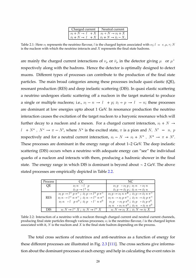
Charged current Neutral currentνl N Ñ l X νl N Ñ νl X

νl N Ñ l X νl N Ñ νl X ,

Table 2.1: Here νl represents the neutrino flavour, l is the charged lepton associated with νl; l e, µ, τ ; Nis the nucleon with which the neutrino interacts andX represents the final state hadrons.

are mainly the charged current interactions of νµ or νµ in the detector giving µ or µ

respectively along with the hadrons. Hence the detector is optimally designed to detect

muons. Different types of processes can contribute to the production of the final state

particles. The main broad categories among these processes include quasi elastic (QE),

resonant production (RES) and deep inelastic scattering (DIS). In quasi elastic scattering

a neutrino undergoes elastic scattering off a nucleon in the target material to produce

a single or multiple nucleons; i.e., νl n Ñ l p; νl p Ñ l n; these processes

are dominant at low energies upto about 1 GeV. In resonance production the neutrino

interaction causes the excitation of the target nucleon to a baryonic resonance which will

further decay to a nucleon and a meson. For a charged current interaction, νl N Ñ

l N , N

Ñ π N 1, where N is the excited state, π is a pion and N, N 1

n, p

respectively and for a neutral current interaction, νl N Ñ νl N , N

Ñ π N 1.

These processes are dominant in the energy range of about 1–2 GeV. The deep inelastic

scattering (DIS) occurs when a neutrino with adequate energy can “see” the individual

quarks of a nucleon and interacts with them, producing a hadronic shower in the final

state. The energy range in which DIS is dominant is beyond about 2 GeV. The above

stated processes are empirically depicted in Table 2.2.

Process CC NCQE νl nÑ l p νl pÑ νl p ; νl nÑ νl n

νl pÑ l n νl pÑ νl p ; νl nÑ νl n

νl pÑ l p π ; νl pÑ l p π νl pÑ νl n π ; νl pÑ νl n π

RES νl nÑ l n π ; νl nÑ l n π νl nÑ νl p π ; νl nÑ νl p π

νl nÑ l p π0 ; νl pÑ l n π0 νl pÑ νl p π0 ; νl pÑ νl p π0

νl nÑ νl n π0 ; νl nÑ νl n π0

DIS νl N Ñ l X ; νl N Ñ l X νl N Ñ νl X ; νl N Ñ νl X

Table 2.2: Interaction of a neutrino with a nucleon through charged current and neutral current channels,producing final state particles through various processes; νl is the neutrino flavour, l is the charged leptonassociated with it, N is the nucleon andX is the final state hadron depending on the process.

The total cross sections of neutrinos and anti-neutrinos as a function of energy for

these different processes are illustrated in Fig. 2.3 [111]. The cross sections give informa-

tion about the dominant processes at each energy and help in calculating the event rates in

28

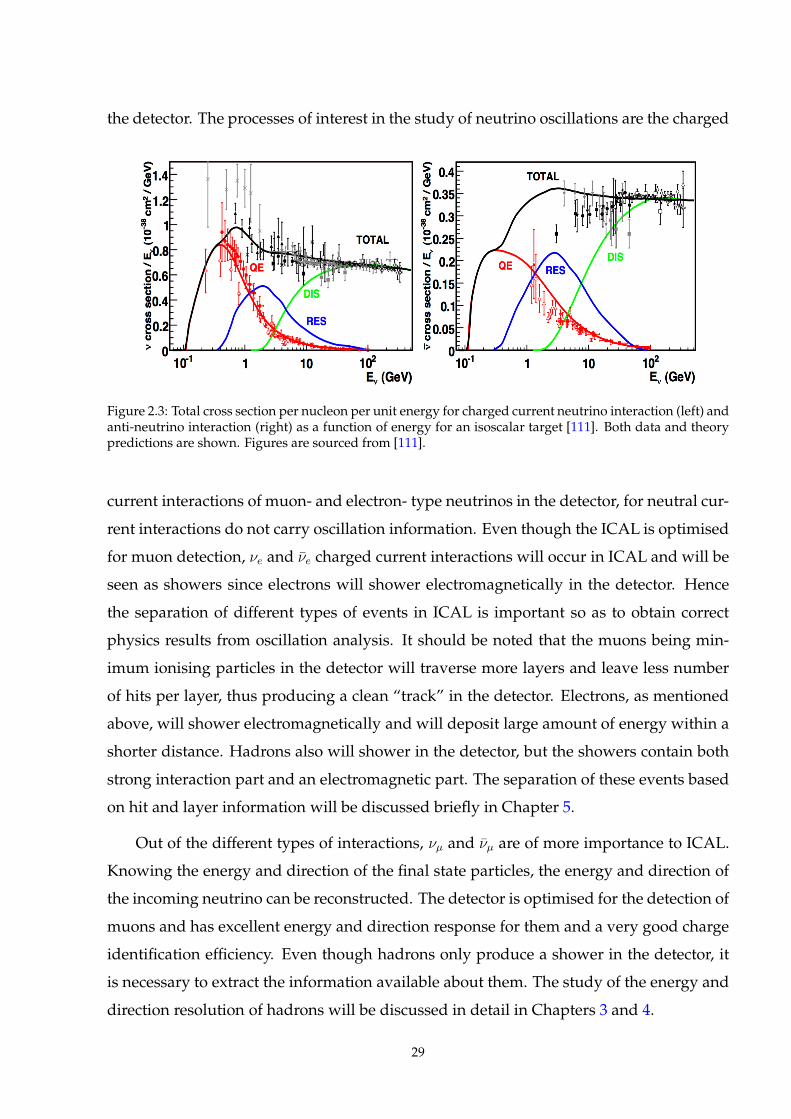
the detector. The processes of interest in the study of neutrino oscillations are the charged

Figure 2.3: Total cross section per nucleon per unit energy for charged current neutrino interaction (left) andanti-neutrino interaction (right) as a function of energy for an isoscalar target [111]. Both data and theorypredictions are shown. Figures are sourced from [111].

current interactions of muon- and electron- type neutrinos in the detector, for neutral cur-

rent interactions do not carry oscillation information. Even though the ICAL is optimised

for muon detection, νe and νe charged current interactions will occur in ICAL and will be

seen as showers since electrons will shower electromagnetically in the detector. Hence

the separation of different types of events in ICAL is important so as to obtain correct

physics results from oscillation analysis. It should be noted that the muons being min-

imum ionising particles in the detector will traverse more layers and leave less number

of hits per layer, thus producing a clean “track” in the detector. Electrons, as mentioned

above, will shower electromagnetically and will deposit large amount of energy within a

shorter distance. Hadrons also will shower in the detector, but the showers contain both

strong interaction part and an electromagnetic part. The separation of these events based

on hit and layer information will be discussed briefly in Chapter 5.

Out of the different types of interactions, νµ and νµ are of more importance to ICAL.

Knowing the energy and direction of the final state particles, the energy and direction of

the incoming neutrino can be reconstructed. The detector is optimised for the detection of

muons and has excellent energy and direction response for them and a very good charge

identification efficiency. Even though hadrons only produce a shower in the detector, it

is necessary to extract the information available about them. The study of the energy and

direction resolution of hadrons will be discussed in detail in Chapters 3 and 4.

29

2.5 Atmospheric neutrino fluxes in ICAL

The source of neutrinos in ICAL is the Earth’s atmosphere. Hence it is important to know

about the flux of these neutrinos since it will eventually determine themass of the detector

and the exposure time required to collect enough number of events to perform neutrino

oscillation studies. These neutrinos are produced by the decay of the secondary cosmic

rays produced in the Earth’s atmosphere when primary cosmic rays, mainly protons from

galactic and extra-galactic sources, impinge on the Earth. Thus the flux of the atmospheric

neutrinos depend upon the flux of these primary cosmic rays and their energies. The

details of neutrino production are described in Section 2.5.1.

2.5.1 Atmospheric neutrino production mechanism

The production of atmospheric neutrinos was explained briefly in Section 1.2.1. The

mechanism is explained again but in detailed in this section. The primary cosmic rays

consist of high energy particles produced in both galactic and extra-galactic sources. Their

energy spectrum extends to very high energies, even beyond 1010 GeV, but falls very

rapidly with the increase in energy. In the GeV energy range, the primary cosmic rays

comprises mainly protons, 9% helium nuclei and a small fraction of heavy nuclei. These

primary cosmic rays interact with the nuclei of the air molecules to produce secondary

cosmic rays (mesons) mainly consisting of pions and a small fraction of kaons. These par-

ticles decay mainly into muons and associated neutrinos according to the decay chain:

π Ñ µ νµpνµq; (2.2)

µ Ñ e νµpνµq νepνeq, (2.3)

where, π represent the charged pions, µ anti-muon and muon, e represent positron

and electron and ν and ν represent neutrino and anti-neutrino respectively.

Similarly, kaons also decay producing the two neutrino flavours νµ and νe, but their

contribution to the atmospheric neutrino flux in the few GeV energy range is small com-

pared to pions. It should be noted that only νµ and νe and their anti-neutrinos are pro-

duced in the atmosphere. The production of ντ requires mesons with heavy quarks to be

produced which results in a negligible flux of ντ in atmospheric neutrinos. Hence, for at-

mospheric neutrino oscillation studies, the relevant neutrino fluxes are those of νµ, νe, νµ

30

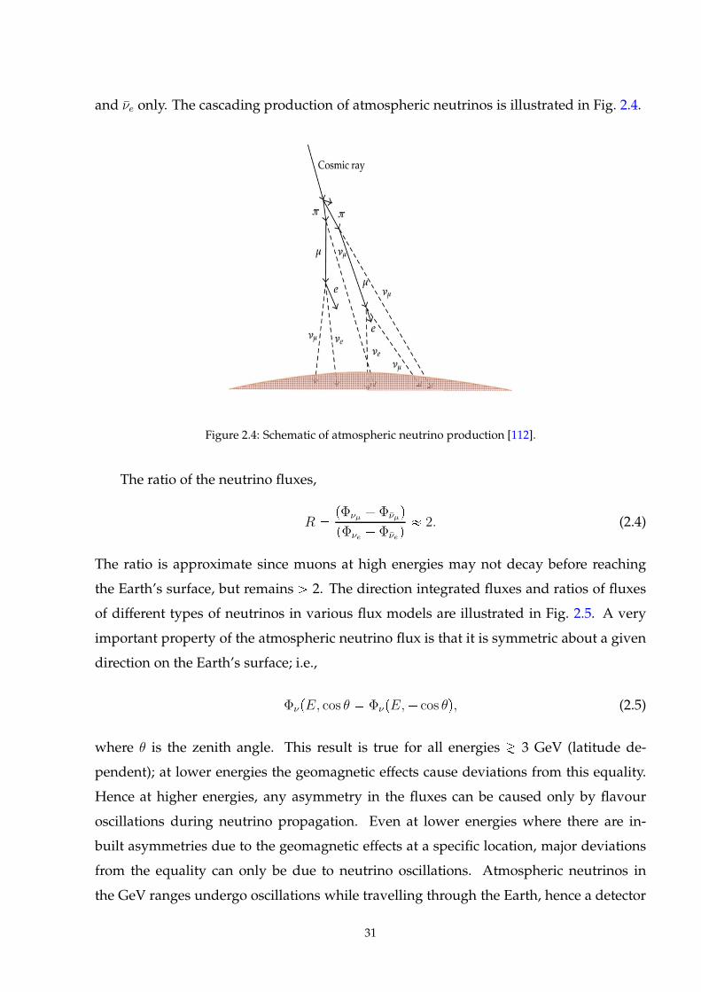
and νe only. The cascading production of atmospheric neutrinos is illustrated in Fig. 2.4.

Figure 2.4: Schematic of atmospheric neutrino production [112].

The ratio of the neutrino fluxes,

R

pΦνµ Φνµq

pΦνe Φνeq 2. (2.4)

The ratio is approximate since muons at high energies may not decay before reaching

the Earth’s surface, but remains ¡ 2. The direction integrated fluxes and ratios of fluxes

of different types of neutrinos in various flux models are illustrated in Fig. 2.5. A very

important property of the atmospheric neutrino flux is that it is symmetric about a given

direction on the Earth’s surface; i.e.,

ΦνpE, cos θ ΦνpE, cos θq, (2.5)

where θ is the zenith angle. This result is true for all energies Á 3 GeV (latitude de-

pendent); at lower energies the geomagnetic effects cause deviations from this equality.

Hence at higher energies, any asymmetry in the fluxes can be caused only by flavour

oscillations during neutrino propagation. Even at lower energies where there are in-

built asymmetries due to the geomagnetic effects at a specific location, major deviations

from the equality can only be due to neutrino oscillations. Atmospheric neutrinos in

the GeV ranges undergo oscillations while travelling through the Earth, hence a detector

31

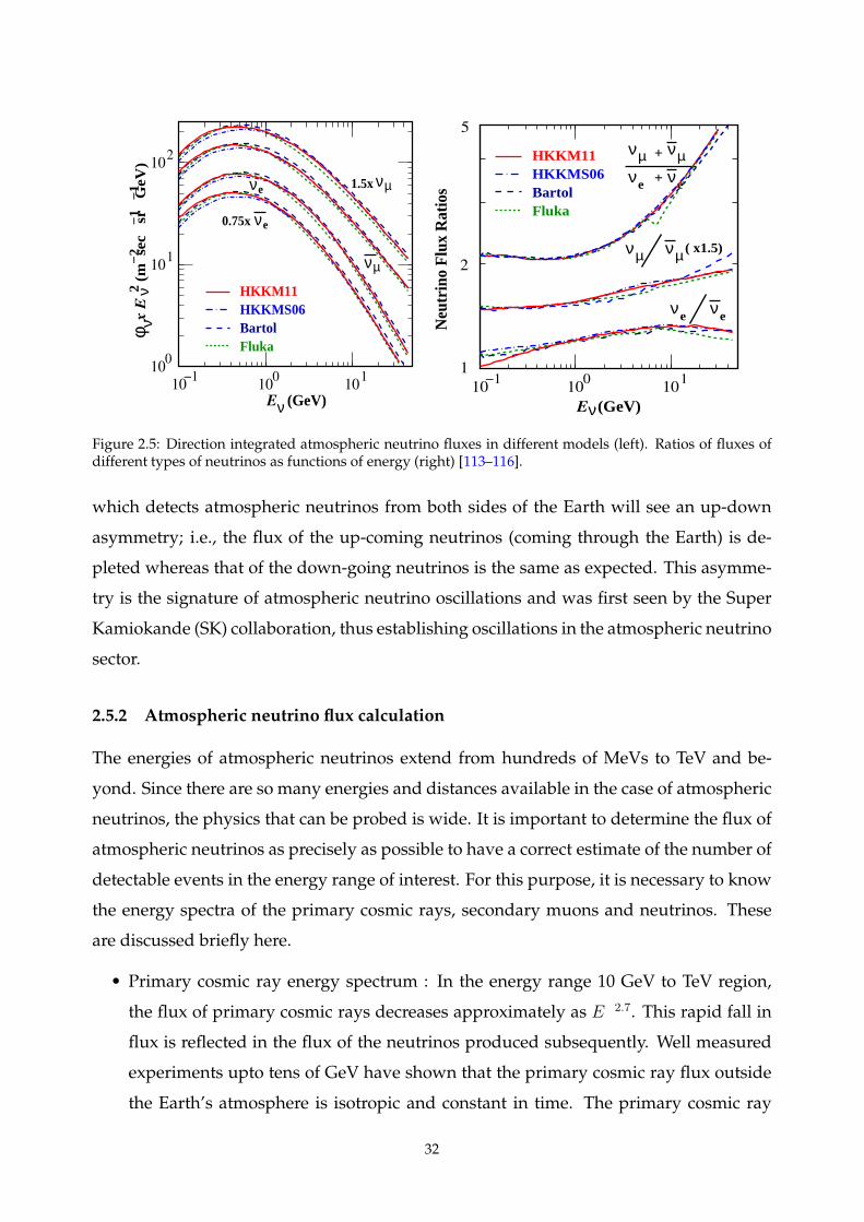
φ ν−

2−

1−

1x E

2 ν(m

se

c

sr

Ge

V)

(GeV)νE

HKKM11HKKMS06BartolFluka

νe0.75x

νe

νµ

µν1.5x

10 −1

100

10 1

100

10 1

10 2 +

+

µνµν

νe νe

νE (GeV)

νeνe

µν µν

Neu

trin

o F

lux

Rat

ios

HKKMS06BartolFluka

HKKM11

( x1.5)

1

10 −1

100

10 1

2

5

Figure 2.5: Direction integrated atmospheric neutrino fluxes in different models (left). Ratios of fluxes ofdifferent types of neutrinos as functions of energy (right) [113–116].

which detects atmospheric neutrinos from both sides of the Earth will see an up-down

asymmetry; i.e., the flux of the up-coming neutrinos (coming through the Earth) is de-

pleted whereas that of the down-going neutrinos is the same as expected. This asymme-

try is the signature of atmospheric neutrino oscillations and was first seen by the Super

Kamiokande (SK) collaboration, thus establishing oscillations in the atmospheric neutrino

sector.

2.5.2 Atmospheric neutrino flux calculation

The energies of atmospheric neutrinos extend from hundreds of MeVs to TeV and be-

yond. Since there are so many energies and distances available in the case of atmospheric

neutrinos, the physics that can be probed is wide. It is important to determine the flux of

atmospheric neutrinos as precisely as possible to have a correct estimate of the number of

detectable events in the energy range of interest. For this purpose, it is necessary to know

the energy spectra of the primary cosmic rays, secondary muons and neutrinos. These

are discussed briefly here.

• Primary cosmic ray energy spectrum : In the energy range 10 GeV to TeV region,

the flux of primary cosmic rays decreases approximately as E2.7. This rapid fall in

flux is reflected in the flux of the neutrinos produced subsequently. Well measured

experiments upto tens of GeV have shown that the primary cosmic ray flux outside

the Earth’s atmosphere is isotropic and constant in time. The primary cosmic ray

32

proton spectrum can be fitter to a form

ΦpEq K

E b exp

c?

Eα

, (2.6)

where, α 2.74,K 14900, b 2.15 and c 0.21 [117].

• Secondary muon spectrum : The primary cosmic rays interacting with the air nuclei

produce pions and kaons which decay to muons. The main input to the calculation

of their fluxes are the hadronic cross sections. These cross sections have been mea-

sured well in the lower energy region upto hundred GeV by accelerator experiments.

Those beyond the energies of accelerators are model dependent. Thus the composi-

tion of the secondary cosmic rays and their energy spectrum is well known upto TeV

energies. This gives a good insight into the energy spectrum of the secondary muons

produced by the decay of these mesons.

• Energy spectrum of atmospheric neutrinos: The atmospheric neutrinos which are

produced during the decay of the secondary muons, in turn will depend on the

properties of all the parent particles and their fluxes. To calculate the energy spec-

trum of these neutrinos, modelling of the interactions in the atmosphere according

to altitude, impact of geomagnetic effects on cosmic ray and secondary fluxes and

dependence of extensive air showers on longitude have to be done.

The precision with which the atmospheric neutrino flux on the Earth’s surface can be

determined is limited by the uncertainties in each of the above steps. As a result, an

uncertainty of the order of 15–20% is introduced in the overall normalization.

It is interesting to see the zenith angle distributions of unoscillated atmospheric neu-

trinos at different energies. The fluxes averaged over azimuthal angles for three neutrino

energies, calculated for Kamioka where the Super Kamiokande (SK) detector is situated,

are shown in Fig. 2.6. From the figure it is evident that the flux is typically maximum

in the cos θ 0 direction, which is the horizontal direction. The muons have maximum

proper time to decay in this direction leading to an increased number of neutrinos as

compared to the other directions. It can also be seen that the ratio of the muon to electron

neutrino flux also increases with the increase in energy and where the direction is more

vertical (for up-coming or down-going neutrinos). This is because the muons have less

proper time to decay thus making the second process in Eq. 2.3 less efficient. Another

33

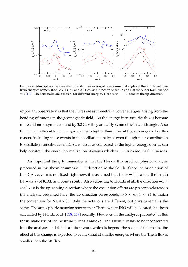
νe

cos θ

φ ν−1

−1−2

(m s

sr

GeV

)−1

νµ

νµ

4x

4x

0.32 GeV

νe

−1.0 −0.50 0 0.50 1.0

10 3

10 3

10 3

10 2

cos θ

φ ν−1

−1−2

(m s

sr

GeV

)−1

νe

νe

νµ

νµ

3x

3x

1.0 GeV

−1.0 −0.50 0 0.50 1.0

10 2

10 2

10 2

10 1

cos θ

φ ν−1

−1−2

(m s

sr

GeV

)−1

νe

νe5x

2x

νµ

νµ

3.2 GeV

10 1

10 0

010

−1.0 −0.50 0 0.50 1.0

10 1

Figure 2.6: Atmospheric neutrino flux distributions averaged over azimuthal angles at three different neu-trino energies namely 0.32 GeV, 1 GeV and 3.2 GeV, as a function of zenith angle at the Super Kamiokandesite [117]. The flux scales are different for different energies. Here cos θ 1 denotes the up-direction.

important observation is that the fluxes are asymmetric at lower energies arising from the

bending of muons in the geomagnetic field. As the energy increases the fluxes become

more and more symmetric and by 3.2 GeV they are fairly symmetric in zenith angle. Also

the neutrino flux at lower energies is much higher than those at higher energies. For this

reason, including these events in the oscillation analyses even though their contribution

to oscillation sensitivities in ICAL is lesser as compared to the higher energy events, can

help constrain the overall normalization of events which will in turn reduce fluctuations.

An important thing to remember is that the Honda flux used for physics analysis

presented in this thesis assumes φ 0 direction as the South. Since the orientation of

the ICAL cavern is not fixed right now, it is assumed that the φ 0 is along the length

(X axis) of ICAL and points south. Also according to Honda et al., the direction 1 ¤

cos θ ¤ 0 is the up-coming direction where the oscillation effects are present, whereas in

the analysis, presented here, the up direction corresponds to 0 ¤ cos θ ¤ 1 to match

the convention for NUANCE. Only the notations are different, but physics remains the

same. The atmospheric neutrino spectrum at Theni, where INO will be located, has been

calculated by Honda et al. [118, 119] recently. However all the analyses presented in this

thesis make use of the neutrino flux at Kamioka. The Theni flux has to be incorporated

into the analyses and this is a future work which is beyond the scope of this thesis. the

effect of this change is expected to be maximal at smaller energies where the Theni flux is

smaller than the SK flux.

34

2.6 Neutrino oscillations relevant to ICAL

The main aim of ICAL detector is to determine the mass hierarchy of neutrinos by study-

ing Earth matter effects during the passage of atmospheric neutrinos through the Earth.

It also aims to study the precision measurement of the oscillation parameters θ23 and

|∆m232|. The physics probed by the ICAL will be discussed in this section.

The main aim of ICAL detector is to determine the neutrino mass hierarchy by prob-

ing the Earth matter effects. Due to matter effects all the oscillation parameters will be

modified in matter as shown in Chapter 1. Since atmospheric neutrinos contain both νµ

and νe in the ratio 2:1, there are many channels of oscillation available for study. Thus

the probabilities Pµµ, Peµ, Pµe and Pµτ and the corresponding anti-neutrino probabilities

are relevant in atmospheric neutrino oscillations. These probabilities and matter effects

at fixed neutrino energies for normal hierarchy have been illustrated in Fig. 1.2. Depend-

ing on the detector resolutions, events from different channels can be detected with high

efficiencies. In the case of ICAL, the detector is optimised for muon detection. Hence

ICAL is most sensitive to νµ Ñ νµ and νe Ñ νµ and the νµ Ñ νµ and νe Ñ νµ channels

in which the final state of oscillation is a νµ or νµ. These νµ and νµ will interact with the

iron in the detector through charged current interactions to give muons and hadrons in

the final state. Since muons are minimum ionising particles at these energies, even with

the detector configuration of 5.6 cm thick iron plates, they travel long distances in the

detector and give a long track bent by the magnetic field according to the charge of the

muon. The momentum and direction of these muons can be reconstructed using Kalman

filter technique.

Hence it can be said that the ICAL is mainly sensitive to Pµµ, Peµ, Pµµ and Peµ. The

interactions of νe and νe with iron can happen thus giving electrons, but currently the

responses of electrons in ICAL have not been characterised and hence this channel is not

considered in the analysis discussed in this thesis. The νµ Ñ ντ oscillations can also occur

but they are also not considered in the analysis discussed here. The analyses are done

with charged current muon neutrino and muon anti-neutrino events only.

35

2.7 Summary

The ICALdetector has been designed in such away that it is optimised for the detection of

muons. As seen in Section 2.4, hadrons are also produced in these neutrino interactions.

The most important point to remember about the muons and hadrons in ICAL is that

muons leave clean tracks in the detector whereas hadrons leave only a shower in the

detector in which the individual hadrons cannot be seen separately. Hence the effect of

the magnetic field on these hadrons cannot also be observed in ICAL; any such effect will

be washed out by the fact that the shower itself is wide and the hadron responses [20, 21]

are worse compared to muon responses [22, 108] in ICAL. Even then the use of hadron

energy information as an observable in the oscillation analysis improves the sensitivities

tremendously [27]. Hence it is necessary to obtain the energy and direction responses of

hadrons in ICAL. Detailed simulations of the hadron energy and direction responses in

ICAL are presented in Chapters 3 and 4.

Even if the inclusion of hadron energy as a new observable increases the sensitivities

of ICAL to oscillation parameters, these studies have earlier been done in the restricted

energy range of 1–11 GeV of the observed muons. But it is very important to use the

detector to its full potential. Hence a study on the oscillation parameters by extending and

optimising the observed muon energy range is interesting. The detailed discussion about

the effect of extending the energy range of observed muons on oscillation sensitivities of

ICAL is presented in Chapter 6. In addition to extending the energy range, the effect of

constraining the νµ-νµ flux ratio on oscillation sensitivities is also reported. It is seen that

these further improve the precisions obtainable with the ICAL detector. It is worthwhile

noting that despite having a simple geometry and the resolutions as will be discussed in

the upcoming chapters, the physics potential of ICAL is simply awesome because of it

being such a massive detector and most importantly magnetisable. This feature makes

ICAL the best detector which can precisely determine mass hierarchy by making use of a

very simple technique without having to worry about any other complications.

36

Part II

Simulation studies of the ICAL detector in a GEANT-4based framework

3Simulation studies of hadron energy

response of the ICAL

3.1 Overview

Hadrons are produced in the final state during both the charged current and neutral cur-

rent interactions of neutrinos and anti-neutrinos with the iron target in ICAL. To recon-

struct the energy and direction of the incoming νµ and νµ it is essential to reconstruct the

energies and directions of the muons and hadrons. Even though the ICAL detector is

optimised for the detection of muons which leave clean tracks in the detector [22], the

hadrons also leave their information as showers in the detector. Although ICAL cannot

distinguish individual hadrons from one another, it is very important to study the energy

and direction responses of these hadrons since they will provide additional information

which will enhance the sensitivity of the ICAL detector to oscillation parameters [27].

Hadrons play a very crucial role in oscillation studies and it is necessary to extract as

much information from them as possible.

This chapter mainly focuses on the simulation studies of hadron energy response of

the ICAL detector. Detailed discussions on how to use the total number of hits in the

hadron shower to calibrate hadron energy and an appropriate functional form which de-

scribes the hadron hit distributions at various energies are presented. It is also important

to improve the hadron energy resolutions to further improve the sensitivity of the detec-

tor. The study of the effect of varying iron plate thickness on the hadron energy response

is also discussed in detail. A study of the eh ratio of the detector is also performed and

reported in this chapter.

3.2 Hadrons in ICAL

When a neutrino interacts with the target nuclei inside the detector, it produces hadrons

along with the final state lepton in the detector. There are both charged current and neu-

tral current interactions of (anti-)neutrinos mainly via three different processes namely

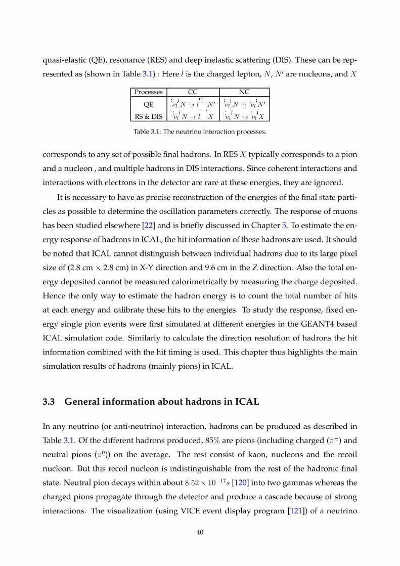
quasi-elastic (QE), resonance (RES) and deep inelastic scattering (DIS). These can be rep-

resented as (shown in Table 3.1) : Here l is the charged lepton, N , N 1 are nucleons, andX

Processes CC NC

QEpq

νl N Ñ lpq

N 1

pq

νl N Ñ

pq

νl N1

RS & DISpq

νl N Ñ lpq

Xpq

νl N Ñ

pq

νl X

Table 3.1: The neutrino interaction processes.

corresponds to any set of possible final hadrons. In RESX typically corresponds to a pion

and a nucleon , and multiple hadrons in DIS interactions. Since coherent interactions and

interactions with electrons in the detector are rare at these energies, they are ignored.

It is necessary to have as precise reconstruction of the energies of the final state parti-

cles as possible to determine the oscillation parameters correctly. The response of muons

has been studied elsewhere [22] and is briefly discussed in Chapter 5. To estimate the en-

ergy response of hadrons in ICAL, the hit information of these hadrons are used. It should

be noted that ICAL cannot distinguish between individual hadrons due to its large pixel

size of (2.8 cm 2.8 cm) in X-Y direction and 9.6 cm in the Z direction. Also the total en-

ergy deposited cannot be measured calorimetrically by measuring the charge deposited.

Hence the only way to estimate the hadron energy is to count the total number of hits

at each energy and calibrate these hits to the energies. To study the response, fixed en-

ergy single pion events were first simulated at different energies in the GEANT4 based

ICAL simulation code. Similarly to calculate the direction resolution of hadrons the hit

information combined with the hit timing is used. This chapter thus highlights the main

simulation results of hadrons (mainly pions) in ICAL.

3.3 General information about hadrons in ICAL

In any neutrino (or anti-neutrino) interaction, hadrons can be produced as described in

Table 3.1. Of the different hadrons produced, 85% are pions (including charged (π) and

neutral pions (π0)) on the average. The rest consist of kaon, nucleons and the recoil

nucleon. But this recoil nucleon is indistinguishable from the rest of the hadronic final

state. Neutral pion decays within about 8.52 1017s [120] into two gammas whereas the

charged pions propagate through the detector and produce a cascade because of strong

interactions. The visualization (using VICE event display program [121]) of a neutrino

40

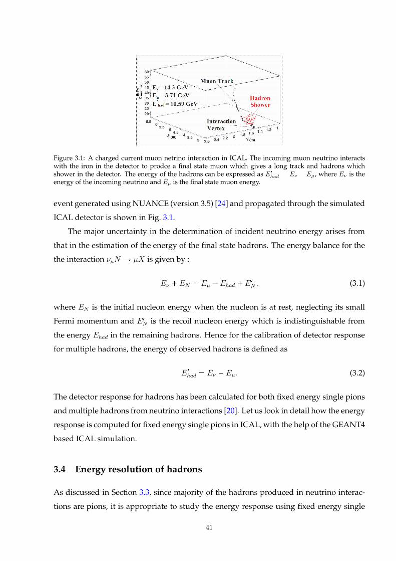
Figure 3.1: A charged current muon netrino interaction in ICAL. The incoming muon neutrino interactswith the iron in the detector to prodce a final state muon which gives a long track and hadrons whichshower in the detector. The energy of the hadrons can be expressed as E1

had Eν Eµ, where Eν is theenergy of the incoming neutrino and Eµ is the final state muon energy.

event generated using NUANCE (version 3.5) [24] and propagated through the simulated

ICAL detector is shown in Fig. 3.1.

The major uncertainty in the determination of incident neutrino energy arises from

that in the estimation of the energy of the final state hadrons. The energy balance for the

the interaction νµN Ñ µX is given by :

Eν EN Eµ Ehad E 1

N , (3.1)

where EN is the initial nucleon energy when the nucleon is at rest, neglecting its small

Fermi momentum and E 1

N is the recoil nucleon energy which is indistinguishable from

the energy Ehad in the remaining hadrons. Hence for the calibration of detector response

for multiple hadrons, the energy of observed hadrons is defined as

E 1

had Eν Eµ. (3.2)

The detector response for hadrons has been calculated for both fixed energy single pions

andmultiple hadrons from neutrino interactions [20]. Let us look in detail how the energy

response is computed for fixed energy single pions in ICAL,with the help of the GEANT4

based ICAL simulation.

3.4 Energy resolution of hadrons

As discussed in Section 3.3, since majority of the hadrons produced in neutrino interac-

tions are pions, it is appropriate to study the energy response using fixed energy single

41

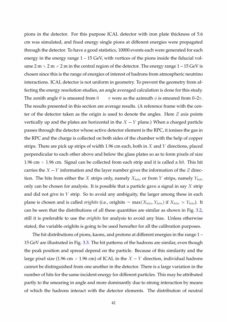
pions in the detector. For this purpose ICAL detector with iron plate thickness of 5.6

cm was simulated, and fixed energy single pions at different energies were propagated

through the detector. To have a good statistics, 10000 events each were generated for each

energy in the energy range 1 – 15 GeV, with vertices of the pions inside the fiducial vol-

ume 2 m 2 m 2 m in the central region of the detector. The energy range 1 – 15 GeV is

chosen since this is the range of energies of interest of hadrons from atmospheric neutrino

interactions. ICAL detector is not uniform in geometry. To prevent the geometry from af-

fecting the energy resolution studies, an angle averaged calculation is done for this study.

The zenith angle θ is smeared from 0 π were as the azimuth φ is smeared from 0–2π.

The results presented in this section are average results. (A reference frame with the cen-

ter of the detector taken as the origin is used to denote the angles. Here Z axis points

vertically up and the plates are horizontal in the X Y plane.) When a charged particle

passes through the detector whose active detector element is the RPC, it ionises the gas in

the RPC and the charge is collected on both sides of the chamber with the help of copper

strips. There are pick up strips of width 1.96 cm each, both in X and Y directions, placed

perpendicular to each other above and below the glass plates so as to form pixels of size

1.96 cm 1.96 cm. Signal can be collected from each strip and it is called a hit. This hit

carries the X Y information and the layer number gives the information of the Z direc-

tion. The hits from either the X strips only, namely Xhits or from Y strips, namely Yhits

only can be chosen for analysis. It is possible that a particle gave a signal in say X strip

and did not give in Y strip. So to avoid any ambiguity, the larger among these in each

plane is chosen and is called orighits (i.e., orighits maxpXhits, Yhitsq if Xhits ¡ Yhits). It

can be seen that the distributions of all these quantities are similar as shown in Fig. 3.2,

still it is preferable to use the orighits for analysis to avoid any bias. Unless otherwise

stated, the variable orighits is going to be used hereafter for all the calibration purposes.

The hit distributions of pions, kaons, and protons at different energies in the range 1 –

15 GeV are illustrated in Fig. 3.3. The hit patterns of the hadrons are similar, even though

the peak position and spread depend on the particle. Because of this similarity and the

large pixel size (1.96 cm 1.96 cm) of ICAL in the X Y direction, individual hadrons

cannot be distinguished from one another in the detector. There is a large variation in the

number of hits for the same incident energy for different particles. This may be attributed

partly to the smearing in angle and more dominantly due to strong interaction by means

of which the hadrons interact with the detector elements. The distribution of neutral

42

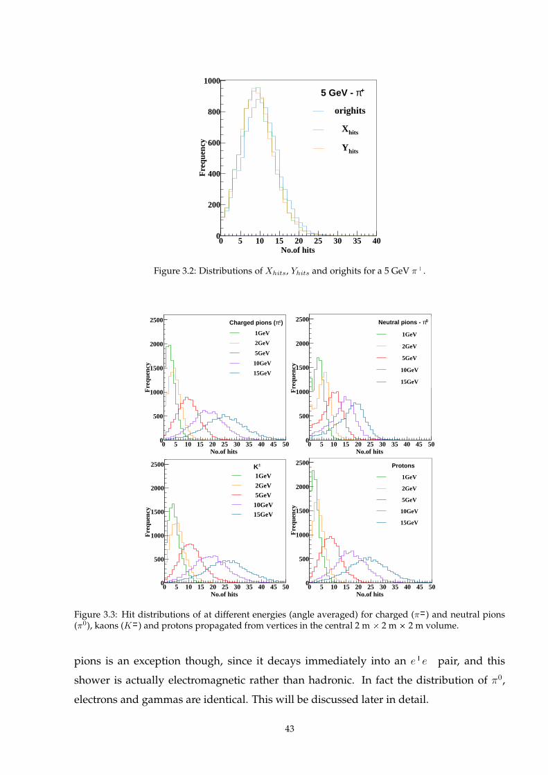
No.of hits 0 5 10 15 20 25 30 35 40

Fre

quen

cy

0

200

400

600

800

1000+π5 GeV -

orighits

hitsX

hitsY

Figure 3.2: Distributions ofXhits, Yhits and orighits for a 5 GeV π.

No.of hits 0 5 10 15 20 25 30 35 40 45 50

Fre

quen

cy

0

500

1000

1500

2000

2500 )±πCharged pions (

1GeV

2GeV

5GeV

10GeV

15GeV

No.of hits 0 5 10 15 20 25 30 35 40 45 50

Fre

quen

cy

0

500

1000

1500

2000

2500 0πNeutral pions -

1GeV

2GeV

5GeV

10GeV

15GeV

No.of hits 0 5 10 15 20 25 30 35 40 45 50

Fre

quen

cy

0

500

1000

1500

2000

2500 ±K1GeV

2GeV

5GeV

10GeV

15GeV

No.of hits 0 5 10 15 20 25 30 35 40 45 50

Fre

quen

cy

0

500

1000

1500

2000

2500 Protons

1GeV

2GeV

5GeV

10GeV

15GeV

Figure 3.3: Hit distributions of at different energies (angle averaged) for charged (π) and neutral pions(π0), kaons (K) and protons propagated from vertices in the central 2 m 2 m 2 m volume.

pions is an exception though, since it decays immediately into an ee pair, and this

shower is actually electromagnetic rather than hadronic. In fact the distribution of π0,

electrons and gammas are identical. This will be discussed later in detail.

43

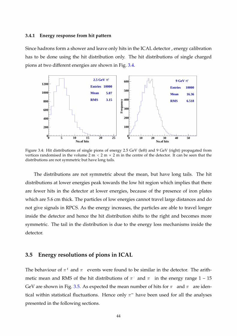
3.4.1 Energy response from hit pattern

Since hadrons form a shower and leave only hits in the ICAL detector , energy calibration

has to be done using the hit distribution only. The hit distributions of single charged

pions at two different energies are shown in Fig. 3.4.

+π2.5 GeV

Entries 10000

Mean 5.07

RMS 3.15

No.of hits0 5 10 15 20 25

0

200

400

600

800

1000

1200

+π2.5 GeV

Entries 10000

Mean 5.07

RMS 3.15

+π9 GeV

Entries 10000

Mean 16.36

RMS 6.518

No.of hits 0 10 20 30 40 50

Fre

quen

cy

0

100

200

300

400

500

600 +π9 GeV

Entries 10000

Mean 16.36

RMS 6.518

Figure 3.4: Hit distributions of single pions of energy 2.5 GeV (left) and 9 GeV (right) propagated fromvertices randomised in the volume 2 m 2 m 2 m in the centre of the detector. It can be seen that thedistributions are not symmetric but have long tails.

The distributions are not symmetric about the mean, but have long tails. The hit

distributions at lower energies peak towards the low hit region which implies that there

are fewer hits in the detector at lower energies, because of the presence of iron plates

which are 5.6 cm thick. The particles of low energies cannot travel large distances and do

not give signals in RPCS. As the energy increases, the particles are able to travel longer

inside the detector and hence the hit distribution shifts to the right and becomes more

symmetric. The tail in the distribution is due to the energy loss mechanisms inside the

detector.

3.5 Energy resolutions of pions in ICAL

The behaviour of π and π events were found to be similar in the detector. The arith-

metic mean and RMS of the hit distributions of π and π in the energy range 1 – 15

GeV are shown in Fig. 3.5. As expected the mean number of hits for π and π are iden-

tical within statistical fluctuations. Hence only π have been used for all the analyses

presented in the following sections.

44

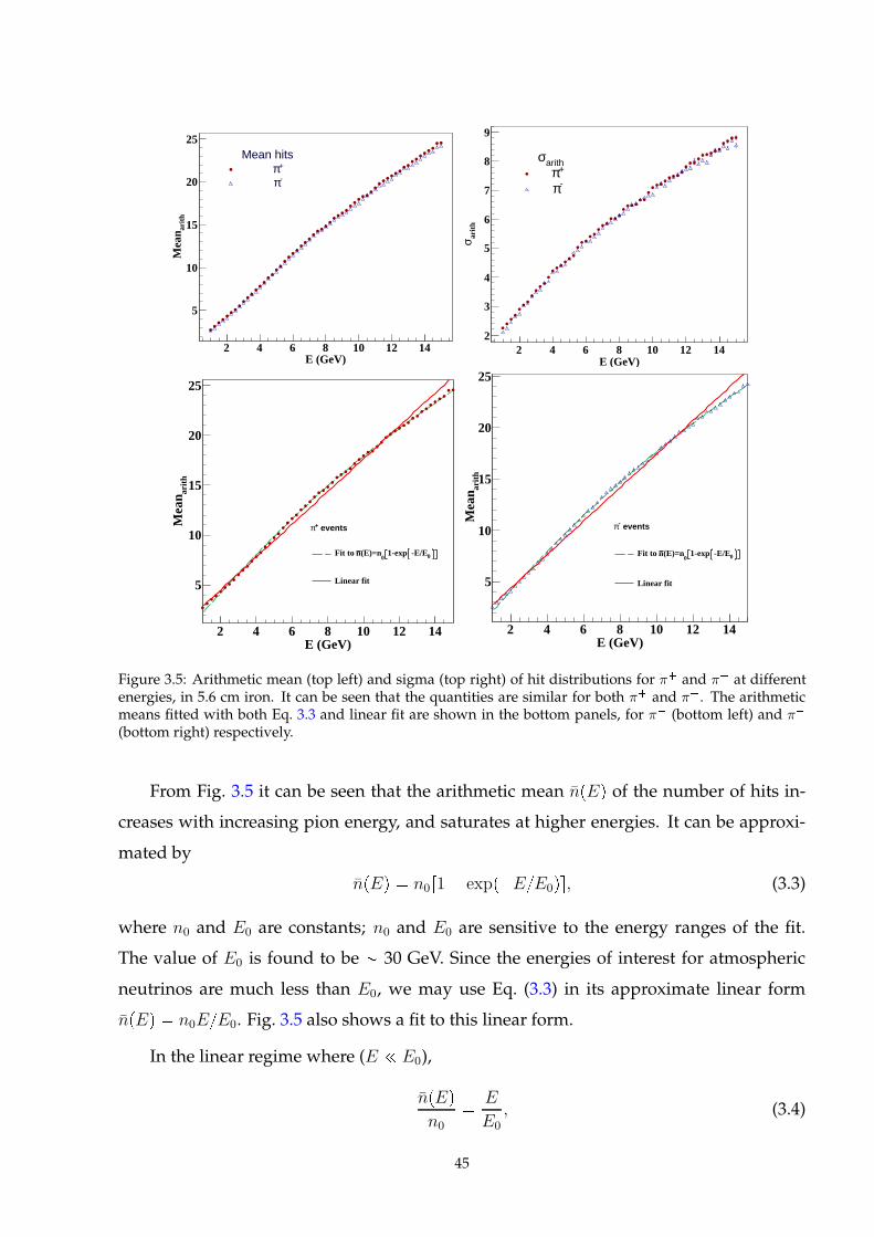
E (GeV)2 4 6 8 10 12 14

arith

Mea

n

5

10

15

20

25Mean hits

+π-π

E (GeV)2 4 6 8 10 12 14

arith

σ

2

3

4

5

6

7

8

9

arithσ+π-π

E (GeV)2 4 6 8 10 12 14

arith

Mea

n

5

10

15

20

25

events+π

0-E/E1-exp0

(E)=nnFit to

Linear fit

E (GeV)2 4 6 8 10 12 14

arith

Mea

n

5

10

15

20

25

events-π

0-E/E1-exp0

(E)=nnFit to

Linear fit

Figure 3.5: Arithmetic mean (top left) and sigma (top right) of hit distributions for π and π at differentenergies, in 5.6 cm iron. It can be seen that the quantities are similar for both π and π. The arithmeticmeans fitted with both Eq. 3.3 and linear fit are shown in the bottom panels, for π (bottom left) and π

(bottom right) respectively.

From Fig. 3.5 it can be seen that the arithmetic mean npEq of the number of hits in-

creases with increasing pion energy, and saturates at higher energies. It can be approxi-

mated by

npEq n0r1 exppEE0qs, (3.3)

where n0 and E0 are constants; n0 and E0 are sensitive to the energy ranges of the fit.

The value of E0 is found to be 30 GeV. Since the energies of interest for atmospheric

neutrinos are much less than E0, we may use Eq. (3.3) in its approximate linear form

npEq n0EE0. Fig. 3.5 also shows a fit to this linear form.

In the linear regime where (E ! E0),

npEq

n0

E

E0

, (3.4)

45

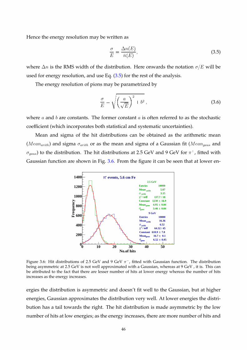
Hence the energy resolution may be written as

σ

E

∆npEq

npEq, (3.5)

where ∆n is the RMS width of the distribution. Here onwards the notation σE will be

used for energy resolution, and use Eq. (3.5) for the rest of the analysis.

The energy resolution of pions may be parametrized by

σ

E

d

a?

E

2

b2 , (3.6)

where a and b are constants. The former constant a is often referred to as the stochastic

coefficient (which incorporates both statistical and systematic uncertainties).

Mean and sigma of the hit distributions can be obtained as the arithmetic mean

(Meanarith) and sigma σarith or as the mean and sigma of a Gaussian fit (Meangaus and

σgaus) to the distribution. The hit distributions at 2.5 GeV and 9 GeV for π, fitted with

Gaussian function are shown in Fig. 3.6. From the figure it can be seen that at lower en-

9 GeVEntries 10000Mean 16.36RMS 6.518

/ ndf 2χ 64.32 / 45Constant 7.8± 610.9 Mean 0.1± 16.7 σ 0.053± 6.522

No.of hits 0 10 20 30 40 50

Fre

quen

cy

0

200

400

600

800

1000

1200

1400

9 GeVEntries 10000Mean arith 16.36σ arith 6.52

/ ndf 2χ 64.32 / 45Constant 7.8± 610.9 Mean gaus 0.1± 16.7 σ gaus 0.05± 6.52

events, 5.6 cm Fe+π2.5 GeV

Entries 10000Mean 5.07RMS 3.15

/ ndf 2χ 137.7 / 18Constant 16.9± 1230 Mean 0.044± 4.948 Sigma 0.044± 3.457

2.5 GeV Entries 10000Mean arith 5.07σ arith 3.15

/ ndf 2χ 137.7 / 18Constant 16.9± 1230 Mean gaus 0.04± 4.95 σ gaus 0.04± 3.46

Figure 3.6: Hit distributions of 2.5 GeV and 9 GeV π, fitted with Gaussian function. The distributionbeing asymmetric at 2.5 GeV is not well approximated with a Gaussian, whereas at 9 GeV , it is. This canbe attributed to the fact that there are lesser number of hits at lower energy whereas the number of hitsincreases as the energy increases.

ergies the distribution is asymmetric and doesn’t fit well to the Gaussian, but at higher

energies, Gaussian approximates the distribution very well. At lower energies the distri-

bution has a tail towards the right. The hit distribution is made asymmetric by the low

number of hits at low energies; as the energy increases, there are more number of hits and

46

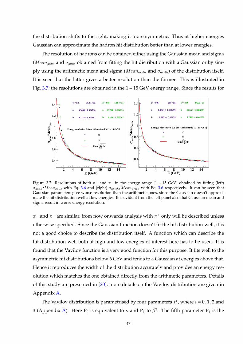
the distribution shifts to the right, making it more symmetric. Thus at higher energies

Gaussian can approximate the hadron hit distribution better than at lower energies.

The resolution of hadrons can be obtained either using the Gaussian mean and sigma

(Meangaus and σgaus obtained from fitting the hit distribution with a Gaussian or by sim-

ply using the arithmetic mean and sigma (Meanarith and σarith) of the distribution itself.

It is seen that the latter gives a better resolution than the former. This is illustrated in

Fig. 3.7; the resolutions are obtained in the 1 – 15 GeV energy range. Since the results for

E (GeV)2 4 6 8 10 12 14

gaus

/Mea

nga

usσ

0.4

0.6

0.8

1

1.2

1.4 / ndf 2χ 360.1 / 55

a 0.004718± 0.9685

b 0.002197± 0.2277

/ ndf 2χ 360.1 / 55

a 0.004718± 0.9685

b 0.002197± 0.2277

/ ndf 2χ 523.4 / 55

a 0.004736± 0.9789

b 0.002267± 0.223

/ ndf 2χ 523.4 / 55

a 0.004736± 0.9789

b 0.002267± 0.223

Energy resolution 5.6 cm - Gaussian Fit [1 - 15 GeV]

+π

-π

2+bE2aFit to

E (GeV)2 4 6 8 10 12 14

arith

/Mea

nar

ithσ

0.4

0.6

0.8

1

1.2

1.4 / ndf 2χ 298 / 55

a 0.003279± 0.8543

b 0.00129± 0.2853

/ ndf 2χ 298 / 55

a 0.003279± 0.8543

b 0.00129± 0.2853

/ ndf 2χ 343.5 / 55

a 0.003289± 0.8558

b 0.001292± 0.2863

/ ndf 2χ 343.5 / 55

a 0.003289± 0.8558

b 0.001292± 0.2863

Energy res o lution 5.6 cm - Arithmetic [1 - 15 GeV]

+π-π

2+bE2aFit to

Figure 3.7: Resolutions of both π and π in the energy range [1 – 15 GeV] obtained by fitting (left)σgausMeangaus with Eq. 3.6 and (right) σarithMeanarith with Eq. 3.6 respectively. It can be seen thatGaussian parameters give worse resolution than the arithmetic ones, since the Gaussian doesn’t approxi-mate the hit distribution well at low energies. It is evident from the left panel also that Gaussian mean andsigma result in worse energy resolution.

π and π are similar, from now onwards analysis with π only will be described unless

otherwise specified. Since the Gaussian function doesn’t fit the hit distribution well, it is

not a good choice to describe the distribution itself. A function which can describe the

hit distribution well both at high and low energies of interest here has to be used. It is

found that the Vavilov function is a very good function for this purpose. It fits well to the

asymmetric hit distributions below 6 GeV and tends to a Gaussian at energies above that.

Hence it reproduces the width of the distribution accurately and provides an energy res-

olution which matches the one obtained directly from the arithmetic parameters. Details

of this study are presented in [20]; more details on the Vavilov distribution are given in

Appendix A.

The Vavilov distribution is parametrised by four parameters Pi, where i = 0, 1, 2 and

3 (Appendix A). Here P0 is equivalent to κ and P1 to β2. The fifth parameter P4 is the

47

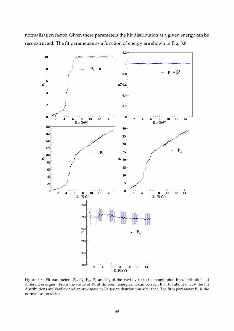
normalisation factor. Given these parameters the hit distribution at a given energy can be

reconstructed. The fit parameters as a function of energy are shown in Fig. 3.8.

(GeV)πE2 4 6 8 10 12 14

0P

0

2

4

6

8

10

κ = 0P

(GeV)πE2 4 6 8 10 12 14

1P

0

0.2

0.4

0.6

0.8

1

1.2

2β = 1P

(GeV)πE2 4 6 8 10 12 14

2P

0

20

40

60

80

100

120

140

160

180

2P

(GeV)πE2 4 6 8 10 12 14

3P

0

5

10

15

20

25

30

35

40

3P

(GeV)πE2 4 6 8 10 12 14

4P

8000

8500

9000

9500

10000

10500

4P

Figure 3.8: Fit parameters P0, P1, P2, P3 and P4 of the Vavilov fit to the single pion hit distributions atdifferent energies. From the value of P0 at different energies, it can be seen that till about 6 GeV the hitdistributions are Vavilov and approximate to Gaussian distribution after that. The fifth parameter P4 is thenormalisation factor.

48

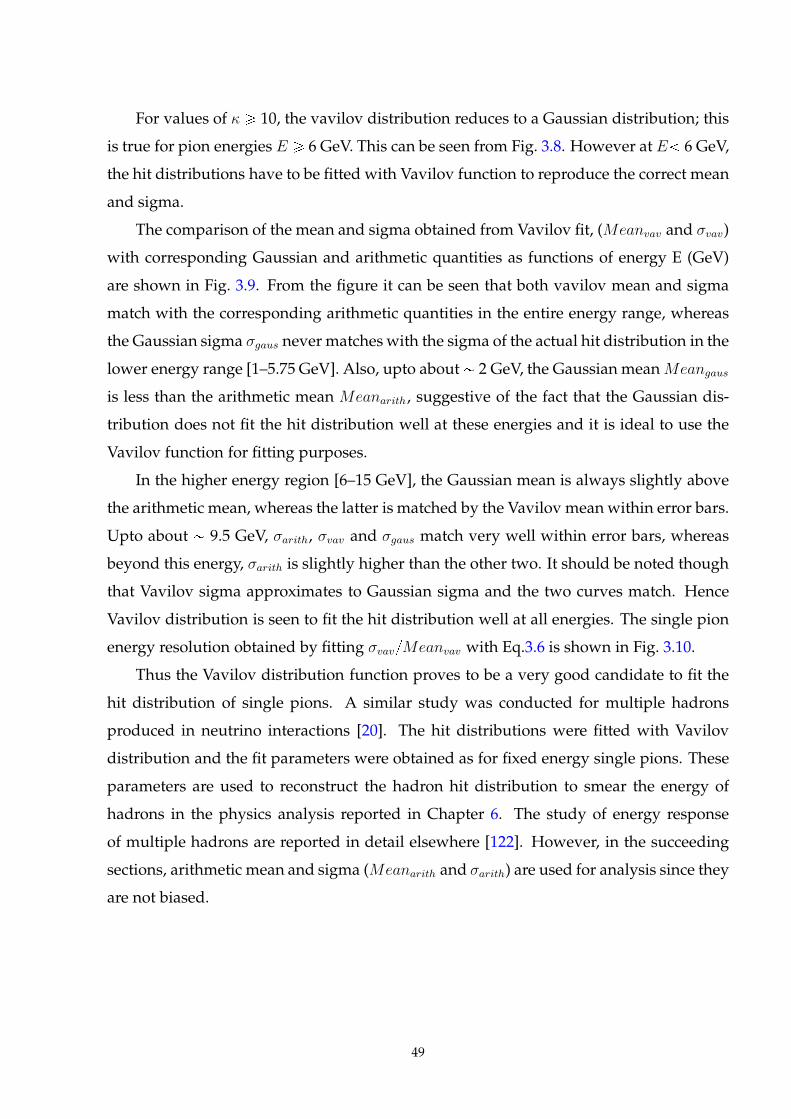
For values of κ ¥ 10, the vavilov distribution reduces to a Gaussian distribution; this

is true for pion energies E ¥ 6 GeV. This can be seen from Fig. 3.8. However at E 6 GeV,

the hit distributions have to be fitted with Vavilov function to reproduce the correct mean

and sigma.

The comparison of the mean and sigma obtained from Vavilov fit, (Meanvav and σvav)

with corresponding Gaussian and arithmetic quantities as functions of energy E (GeV)

are shown in Fig. 3.9. From the figure it can be seen that both vavilov mean and sigma

match with the corresponding arithmetic quantities in the entire energy range, whereas

the Gaussian sigma σgaus never matches with the sigma of the actual hit distribution in the

lower energy range [1–5.75 GeV]. Also, upto about 2 GeV, the Gaussian meanMeangaus

is less than the arithmetic mean Meanarith, suggestive of the fact that the Gaussian dis-

tribution does not fit the hit distribution well at these energies and it is ideal to use the

Vavilov function for fitting purposes.

In the higher energy region [6–15 GeV], the Gaussian mean is always slightly above

the arithmetic mean, whereas the latter is matched by the Vavilov mean within error bars.

Upto about 9.5 GeV, σarith, σvav and σgaus match very well within error bars, whereas

beyond this energy, σarith is slightly higher than the other two. It should be noted though

that Vavilov sigma approximates to Gaussian sigma and the two curves match. Hence

Vavilov distribution is seen to fit the hit distribution well at all energies. The single pion

energy resolution obtained by fitting σvavMeanvav with Eq.3.6 is shown in Fig. 3.10.

Thus the Vavilov distribution function proves to be a very good candidate to fit the

hit distribution of single pions. A similar study was conducted for multiple hadrons

produced in neutrino interactions [20]. The hit distributions were fitted with Vavilov

distribution and the fit parameters were obtained as for fixed energy single pions. These

parameters are used to reconstruct the hadron hit distribution to smear the energy of

hadrons in the physics analysis reported in Chapter 6. The study of energy response

of multiple hadrons are reported in detail elsewhere [122]. However, in the succeeding

sections, arithmetic mean and sigma (Meanarith and σarith) are used for analysis since they

are not biased.

49

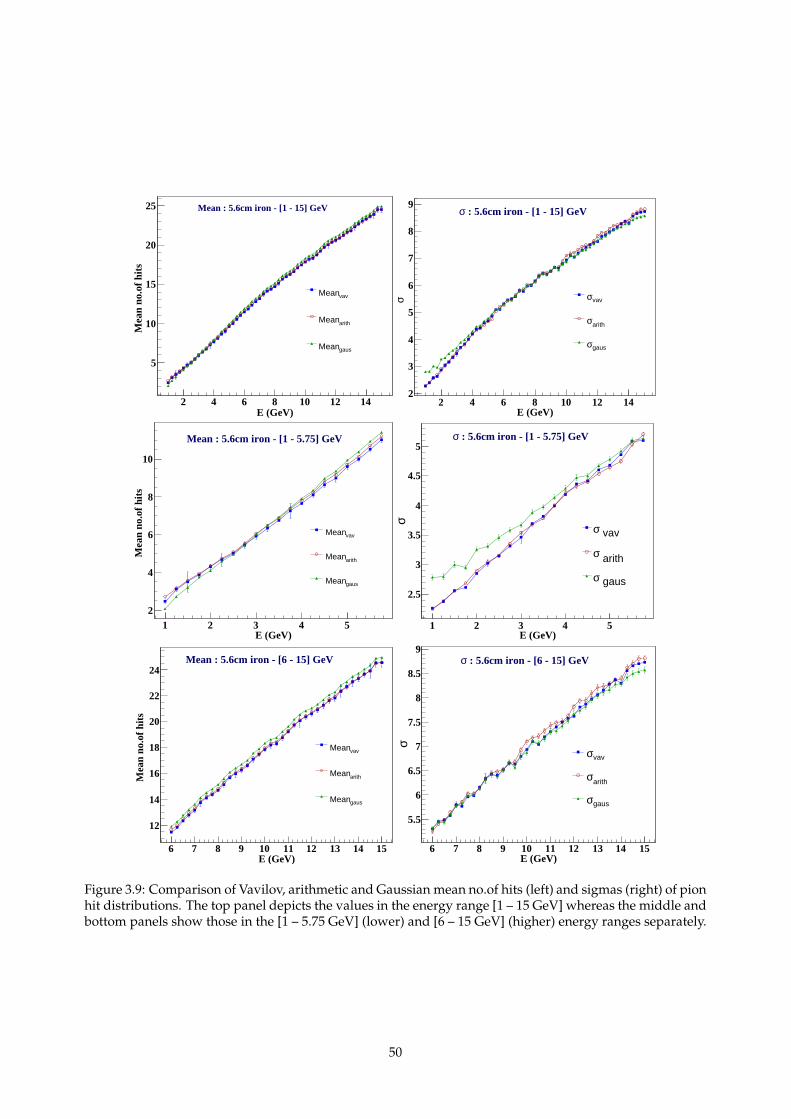
E (GeV)2 4 6 8 10 12 14

Mea

n no

.of h

its

5

10

15

20

25

vavMean

arithMean

gausMean

Mean : 5.6cm iron - [1 - 15] GeV

E (GeV)2 4 6 8 10 12 14

σ2

3

4

5

6

7

8

9

vavσ

arithσ

gausσ

: 5.6cm iron - [1 - 15] GeVσ

E (GeV)1 2 3 4 5

Mea

n no

.of h

its

2

4

6

8

10

vavMean

arithMean

gausMean

Mean : 5.6cm iron - [1 - 5.75] GeV

E (GeV)1 2 3 4 5

σ

2.5

3

3.5

4

4.5

5

vavσ

arithσ

gausσ

: 5.6cm iron - [1 - 5.75] GeVσ

E (GeV)6 7 8 9 10 11 12 13 14 15

Mea

n no

.of h

its

12

14

16

18

20

22

24

vavMean

arithMean

gausMean

Mean : 5.6cm iron - [6 - 15] GeV

E (GeV)6 7 8 9 10 11 12 13 14 15

σ

5.5

6

6.5

7

7.5

8

8.5

9

vavσ

arithσ

gausσ

: 5.6cm iron - [6 - 15] GeVσ

Figure 3.9: Comparison of Vavilov, arithmetic and Gaussian mean no.of hits (left) and sigmas (right) of pionhit distributions. The top panel depicts the values in the energy range [1 – 15 GeV] whereas the middle andbottom panels show those in the [1 – 5.75 GeV] (lower) and [6 – 15 GeV] (higher) energy ranges separately.

50

E (GeV)2 4 6 8 10 12 14

vav

/Mea

nva

vσ

0.4

0.5

0.6

0.7

0.8

0.9

/ ndf 2χ 165.7 / 55

a 0.004552± 0.863

b 0.001707± 0.2801

/ ndf 2χ 165.7 / 55

a 0.005± 0.863

b 0.002± 0.280

vav/Meanvavσ

2+bE2a

E (GeV)1 1.5 2 2.5 3 3.5 4 4.5

vav

/Mea

nva

vσ

0.55

0.6

0.65

0.7

0.75

0.8

0.85 / ndf 2χ 7.202 / 14

a 0.01162± 0.7576

b 0.00926± 0.3866

/ ndf 2χ 7.2 / 14

a 0.012± 0.758

b 0.009± 0.387

[1 - 4.75 GeV]

vav/Meanvavσ

2+bE2a

E (GeV)5 6 7 8 9 10 11 12 13 14 15

vav

vav/

Mea

nσ

0.36

0.38

0.4

0.42

0.44

0.46

0.48 / ndf 2χ 35.78 / 38

a 0.01009± 0.9084

b 0.003401± 0.2656

/ ndf 2χ 35.8 / 38

a 0.01± 0.91

b 0.003± 0.266

[5 - 15 GeV]

vav/Meanvavσ

2+bE2a

Figure 3.10: Energy resolution obtained by fitting σvavMeanvav with Eq. 3.6, in the [1–15 GeV] energyrange. It can be seen that the resolution obtained using Vavilov mean and sigma is similar to that obtainedusing the corresponding arithmetic quantities as shown in Fig. 3.7. The full energy range [1 – 15 GeV] canbe split up into a lower and higher energy range to consider different processes. Bottom left and rightpanels show the energy resolutions in two separate energy ranges namely [1 – 4.75 GeV] which is the lowerenergy range and [5 – 15 GeV], the higher energy range respectively.

51

3.6 Hadron energy resolution as a function of iron plate thickness

This section will deal with the study of dependence of energy resolution on the thickness

of the absorber, which is iron in ICAL, used in the detector. This study is relevant in terms

of improvement of the resolution of hadrons, and thus the information it provides. The

physics reach of INO ICAL is significantly improved by the addition of hadron energy

information, as can be seen in Ref. [27]. Thus hadron energy resolution plays a crucial

role in the study of oscillation parameters with ICAL. Hence it is important to investi-

gate about and implement any possible detector configuration which can add information

thus improving the reach of ICAL. The study of thickness dependence of hadron energy

resolution is one such study in this direction. Even when improving the resolution of the

detector is of interest to the physics to be probed by the ICAL, it is important that it be

cost effective and hence the size, geometry and structural stability of the detector be op-

timised. It is also important that these studies be done specifically for the ICAL detector,

which primarily is an atmospheric neutrino detector, in which the hadrons produced in

the final state have energies of the order of a few GeVs as compared to those detected

by dedicated hadron calorimeters in collider experiments [123–126]. There the hadrons

have energies ranging from tens of GeVs to hundreds of GeVs and these studies indicate

a square root dependence on the thickness t of the hadron energy resolution on the ab-

sorber thickness. The work on the thickness dependence of hadron energy resolution of

the ICAL detector presented here intended to study the effect of plate thickness on the

energy response of hadrons in the few GeV energy range and is of interest to neutrino

experiments, which is otherwise not widely discussed in literature.

The current default geometry of ICAL has 5.6 cm thick iron plates stacked in 151 lay-

ers in the vertical (Z) direction. The total height of ICAL is 14.45 m. For the study of

thickness dependence of hadron energy resolution, 11 thicknesses namely 1.5 cm, 2 cm,

2.5 cm, 3 cm, 3.5 cm, 4 cm, 4.5 cm, 5 cm, 5.6 cm, 6 cm and 8 cm have been considered.

The plate thickness is changed in the GEANT4 simulation code keeping the height of the

detector same. This means that the number of layers will vary accordingly. The simula-

tions study has been conducted using both single pions generated using GEANT4 particle

gun and also hadrons from NUANCE neutrino events. The detailed study presented is

however using single pions. Since arithmetic mean (Meanarith) and sigma (σarith) provide

unbiased results, energy resolutions have been calculated using these quantities using

52

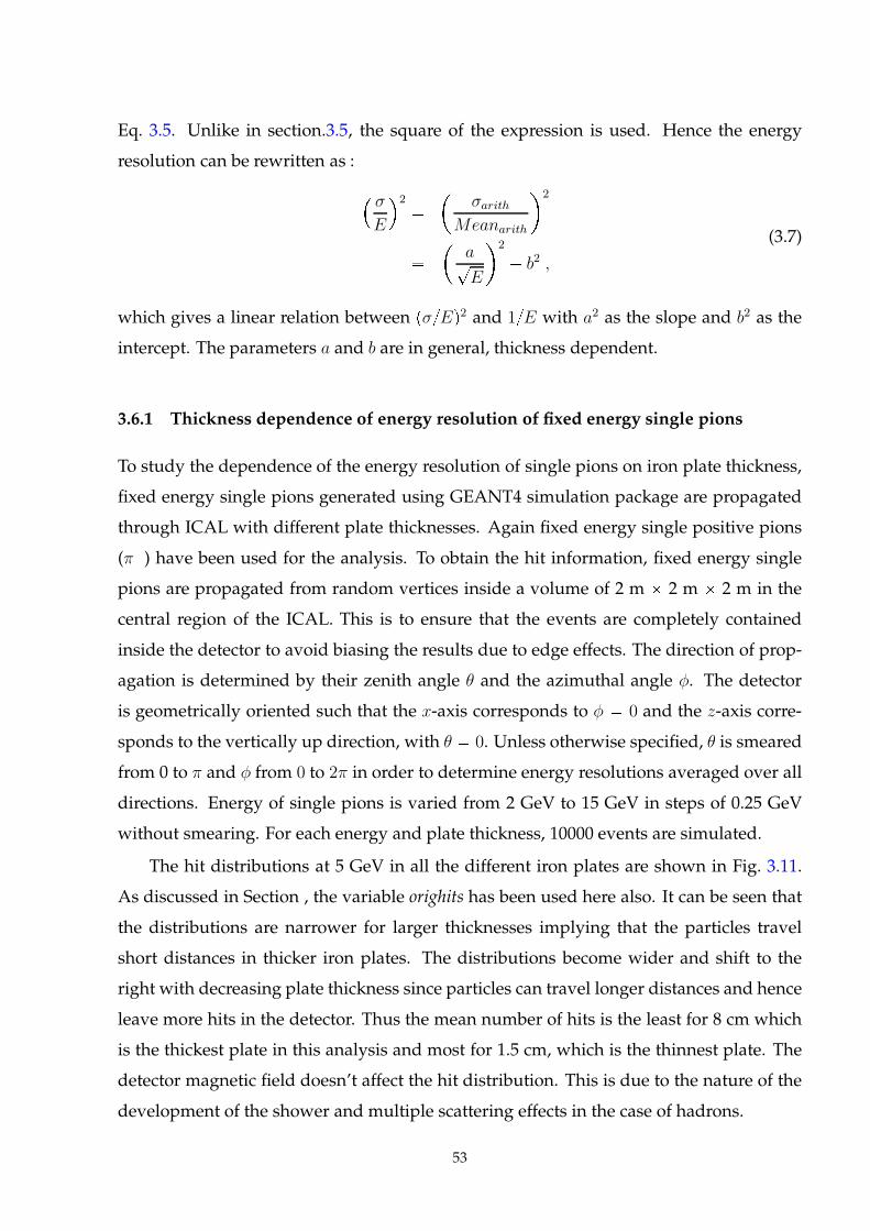
Eq. 3.5. Unlike in section.3.5, the square of the expression is used. Hence the energy

resolution can be rewritten as :

σ

E

2

σarith

Meanarith

2

a?

E

2

b2 ,

(3.7)

which gives a linear relation between pσEq2 and 1E with a2 as the slope and b2 as the

intercept. The parameters a and b are in general, thickness dependent.

3.6.1 Thickness dependence of energy resolution of fixed energy single pions

To study the dependence of the energy resolution of single pions on iron plate thickness,

fixed energy single pions generated using GEANT4 simulation package are propagated

through ICAL with different plate thicknesses. Again fixed energy single positive pions

(π) have been used for the analysis. To obtain the hit information, fixed energy single

pions are propagated from random vertices inside a volume of 2 m 2 m 2 m in the

central region of the ICAL. This is to ensure that the events are completely contained

inside the detector to avoid biasing the results due to edge effects. The direction of prop-

agation is determined by their zenith angle θ and the azimuthal angle φ. The detector

is geometrically oriented such that the x-axis corresponds to φ 0 and the z-axis corre-

sponds to the vertically up direction, with θ 0. Unless otherwise specified, θ is smeared

from 0 to π and φ from 0 to 2π in order to determine energy resolutions averaged over all

directions. Energy of single pions is varied from 2 GeV to 15 GeV in steps of 0.25 GeV

without smearing. For each energy and plate thickness, 10000 events are simulated.

The hit distributions at 5 GeV in all the different iron plates are shown in Fig. 3.11.

As discussed in Section , the variable orighits has been used here also. It can be seen that

the distributions are narrower for larger thicknesses implying that the particles travel

short distances in thicker iron plates. The distributions become wider and shift to the

right with decreasing plate thickness since particles can travel longer distances and hence

leave more hits in the detector. Thus the mean number of hits is the least for 8 cm which

is the thickest plate in this analysis and most for 1.5 cm, which is the thinnest plate. The

detector magnetic field doesn’t affect the hit distribution. This is due to the nature of the

development of the shower and multiple scattering effects in the case of hadrons.

53

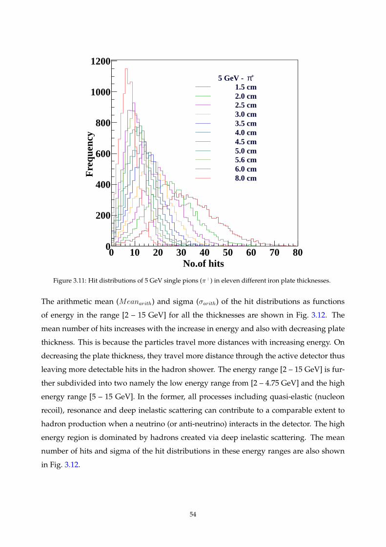
No.of hits 0 10 20 30 40 50 60 70 80

Fre

quen

cy

0

200

400

600

800

1000

1200+π5 GeV -

1.5 cm2.0 cm2.5 cm3.0 cm3.5 cm4.0 cm4.5 cm5.0 cm5.6 cm6.0 cm8.0 cm

Figure 3.11: Hit distributions of 5 GeV single pions (π) in eleven different iron plate thicknesses.

The arithmetic mean (Meanarith) and sigma (σarith) of the hit distributions as functions

of energy in the range [2 – 15 GeV] for all the thicknesses are shown in Fig. 3.12. The

mean number of hits increases with the increase in energy and also with decreasing plate

thickness. This is because the particles travel more distances with increasing energy. On

decreasing the plate thickness, they travel more distance through the active detector thus

leaving more detectable hits in the hadron shower. The energy range [2 – 15 GeV] is fur-

ther subdivided into two namely the low energy range from [2 – 4.75 GeV] and the high

energy range [5 – 15 GeV]. In the former, all processes including quasi-elastic (nucleon

recoil), resonance and deep inelastic scattering can contribute to a comparable extent to

hadron production when a neutrino (or anti-neutrino) interacts in the detector. The high

energy region is dominated by hadrons created via deep inelastic scattering. The mean

number of hits and sigma of the hit distributions in these energy ranges are also shown

in Fig. 3.12.

54

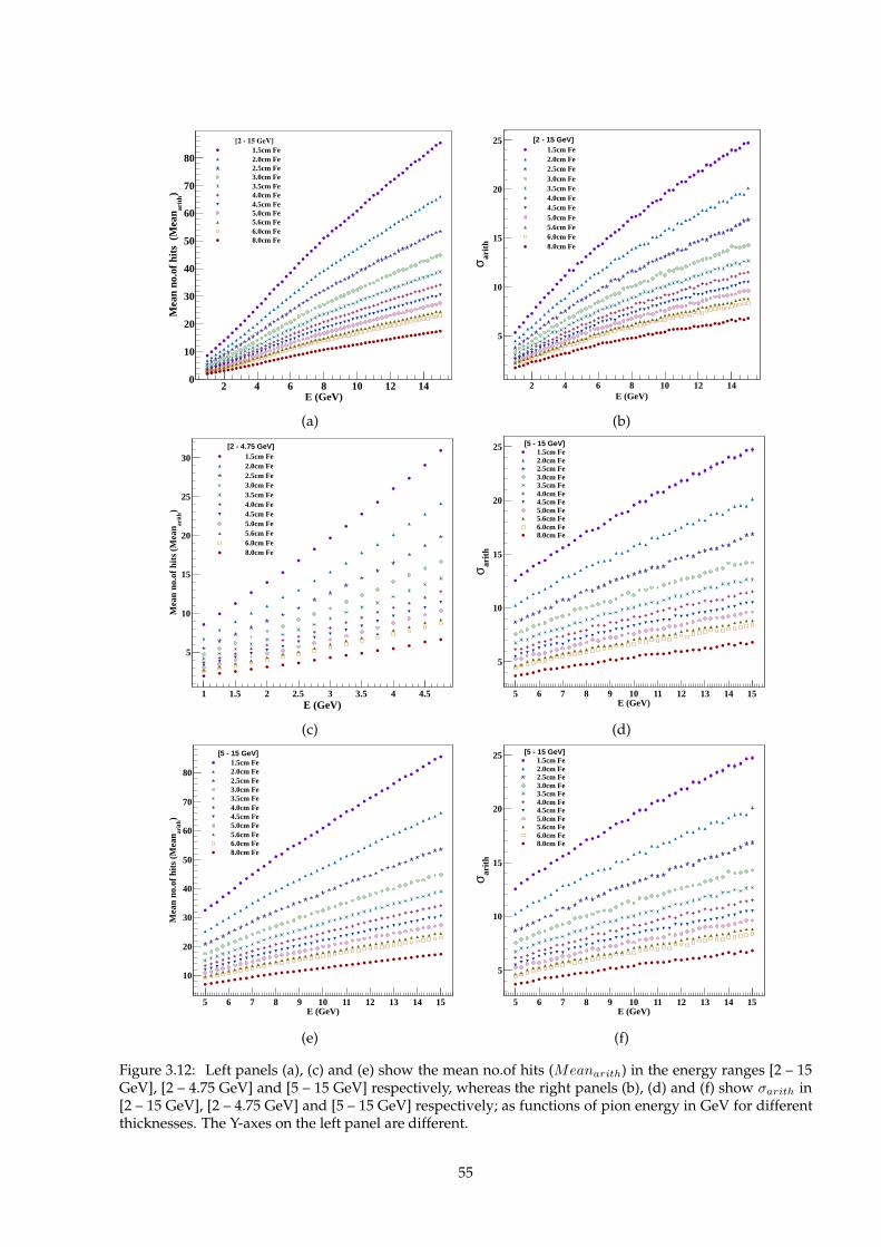
E (GeV)2 4 6 8 10 12 14

)ar

ithM

ean

no.o

f hits

(M

ean

0

10

20

30

40

50

60

70

80

[2 15 GeV]

1.5cm Fe2.0cm Fe2.5cm Fe3.0cm Fe3.5cm Fe4.0cm Fe4.5cm Fe5.0cm Fe5.6cm Fe6.0cm Fe8.0cm Fe

E (GeV)2 4 6 8 10 12 14

arith

σ

5

10

15

20

25 [2 - 15 GeV]1.5cm Fe2.0cm Fe2.5cm Fe3.0cm Fe3.5cm Fe4.0cm Fe4.5cm Fe5.0cm Fe5.6cm Fe6.0cm Fe8.0cm Fe

(a) (b)

E (GeV)1 1.5 2 2.5 3 3.5 4 4.5

)ar

ithM

ean

no.o

f hits

(M

ean

5

10

15

20

25

30[2 - 4.75 GeV]

1.5cm Fe2.0cm Fe2.5cm Fe3.0cm Fe3.5cm Fe4.0cm Fe4.5cm Fe5.0cm Fe5.6cm Fe6.0cm Fe8.0cm Fe

E (GeV)5 6 7 8 9 10 11 12 13 14 15

arith

σ

5

10

15

20


(c) (d)

E (GeV)5 6 7 8 9 10 11 12 13 14 15

)ar

ithM

ean

no.o

f hits

(M

ean

10

20

30

40

50

60

70

80

[5 - 15 GeV]1.5cm Fe2.0cm Fe2.5cm Fe3.0cm Fe3.5cm Fe4.0cm Fe4.5cm Fe5.0cm Fe5.6cm Fe6.0cm Fe8.0cm Fe

E (GeV)5 6 7 8 9 10 11 12 13 14 15

arith

σ

5

10

15

20


(e) (f)

Figure 3.12: Left panels (a), (c) and (e) show the mean no.of hits (Meanarith) in the energy ranges [2 – 15GeV], [2 – 4.75 GeV] and [5 – 15 GeV] respectively, whereas the right panels (b), (d) and (f) show σarith in[2 – 15 GeV], [2 – 4.75 GeV] and [5 – 15 GeV] respectively; as functions of pion energy in GeV for differentthicknesses. The Y-axes on the left panel are different.

55

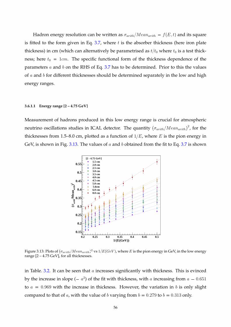
Hadron energy resolution can be written as σarithMeanarith fpE, tq and its square

is fitted to the form given in Eq. 3.7, where t is the absorber thickness (here iron plate

thickness) in cm (which can alternatively be parametrised as tt0 where t0 is a test thick-

ness; here t0 1cm. The specific functional form of the thickness dependence of the

parameters a and b on the RHS of Eq. 3.7 has to be determined. Prior to this the values

of a and b for different thicknesses should be determined separately in the low and high

energy ranges.

3.6.1.1 Energy range [2 – 4.75 GeV]

Measurement of hadrons produced in this low energy range is crucial for atmospheric

neutrino oscillations studies in ICAL detector. The quantity pσarithMeanarithq2, for the

thicknesses from 1.5–8.0 cm, plotted as a function of 1E, where E is the pion energy in

GeV, is shown in Fig. 3.13. The values of a and b obtained from the fit to Eq. 3.7 is shown

1/(E(GeV))0.2 0.25 0.3 0.35 0.4 0.45 0.5

2 )ar

ith/M

ean

arith

σ(

0.15

0.2

0.25

0.3

0.35

0.4

0.45

0.5

0.55

[2 - 4.75 GeV]1.5 cm2.0 cm2.5 cm3.0 cm3.5 cm4.0 cm4.5 cm5.0 cm5.6cm6.0 cm8.0 cm

Figure 3.13: Plots of pσarithMeanarithq2 vs 1EpGeV q, whereE is the pion energy in GeV, in the low energy

range [2 – 4.75 GeV], for all thicknesses.

in Table. 3.2. It can be seen that a increases significantly with thickness. This is evinced

by the increase in slope ( a2) of the fit with thickness, with a increasing from a 0.651

to a 0.969 with the increase in thickness. However, the variation in b is only slight

compared to that of a, with the value of b varying from b 0.279 to b 0.313 only.

56

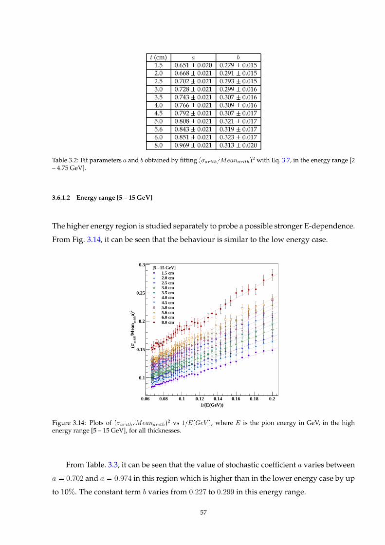
t (cm) a b

1.5 0.651 0.020 0.279 0.0152.0 0.668 0.021 0.291 0.0152.5 0.702 0.021 0.293 0.0153.0 0.728 0.021 0.299 0.0163.5 0.743 0.021 0.307 0.0164.0 0.766 0.021 0.309 0.0164.5 0.792 0.021 0.307 0.0175.0 0.808 0.021 0.321 0.0175.6 0.843 0.021 0.319 0.0176.0 0.851 0.021 0.323 0.0178.0 0.969 0.021 0.313 0.020

Table 3.2: Fit parameters a and b obtained by fitting pσarithMeanarithq2 with Eq. 3.7, in the energy range [2

– 4.75 GeV].

3.6.1.2 Energy range [5 – 15 GeV]

The higher energy region is studied separately to probe a possible stronger E-dependence.

From Fig. 3.14, it can be seen that the behaviour is similar to the low energy case.

1/(E(GeV))0.06 0.08 0.1 0.12 0.14 0.16 0.18 0.2

2a)

arith

/Mea

nar

ithσ(

0.1

0.15

0.2

0.25

0.3[5 - 15 GeV]


Figure 3.14: Plots of pσarithMeanarithq2 vs 1EpGeV q, where E is the pion energy in GeV, in the high

energy range [5 – 15 GeV], for all thicknesses.

From Table. 3.3, it can be seen that the value of stochastic coefficient a varies between

a 0.702 and a 0.974 in this region which is higher than in the lower energy case by up

to 10%. The constant term b varies from 0.227 to 0.299 in this energy range.

57

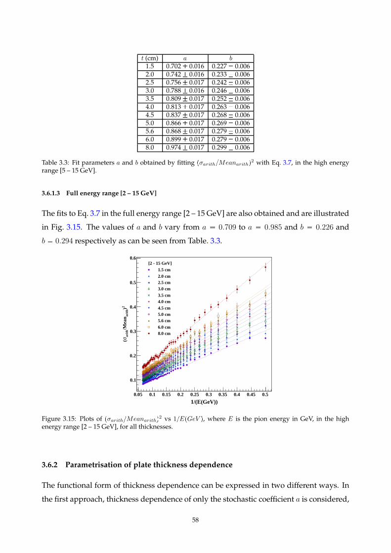
t (cm) a b

1.5 0.702 0.016 0.227 0.0062.0 0.742 0.016 0.233 0.0062.5 0.756 0.017 0.242 0.0063.0 0.788 0.016 0.246 0.0063.5 0.809 0.017 0.252 0.0064.0 0.813 0.017 0.263 0.0064.5 0.837 0.017 0.268 0.0065.0 0.866 0.017 0.269 0.0065.6 0.868 0.017 0.279 0.0066.0 0.899 0.017 0.279 0.0068.0 0.974 0.017 0.299 0.006

Table 3.3: Fit parameters a and b obtained by fitting pσarithMeanarithq2 with Eq. 3.7, in the high energy

range [5 – 15 GeV].

3.6.1.3 Full energy range [2 – 15 GeV]

The fits to Eq. 3.7 in the full energy range [2 – 15 GeV] are also obtained and are illustrated

in Fig. 3.15. The values of a and b vary from a 0.709 to a 0.985 and b 0.226 and

b 0.294 respectively as can be seen from Table. 3.3.

1/(E(GeV))0.05 0.1 0.15 0.2 0.25 0.3 0.35 0.4 0.45 0.5

2 )ar

ith/M

ean

arith

σ(

0.1

0.2

0.3

0.4

0.5

0.6[2 - 15 GeV]


Figure 3.15: Plots of pσarithMeanarithq2 vs 1EpGeV q, where E is the pion energy in GeV, in the high

energy range [2 – 15 GeV], for all thicknesses.

3.6.2 Parametrisation of plate thickness dependence

The functional form of thickness dependence can be expressed in two different ways. In

the first approach, thickness dependence of only the stochastic coefficient a is considered,

58

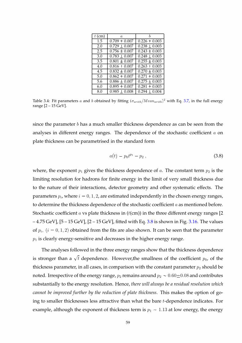
t (cm) a b

1.5 0.709 0.007 0.226 0.0032.0 0.729 0.007 0.238 0.0032.5 0.756 0.007 0.243 0.0033.0 0.783 0.007 0.248 0.0033.5 0.801 0.007 0.255 0.0034.0 0.816 0.007 0.263 0.0034.5 0.832 0.007 0.270 0.0035.0 0.862 0.007 0.271 0.0035.6 0.886 0.007 0.275 0.0036.0 0.895 0.007 0.281 0.0038.0 0.985 0.008 0.294 0.004

Table 3.4: Fit parameters a and b obtained by fitting pσarithMeanarithq2 with Eq. 3.7, in the full energy

range [2 – 15 GeV].

since the parameter b has a much smaller thickness dependence as can be seen from the

analyses in different energy ranges. The dependence of the stochastic coefficient a on

plate thickness can be parametrised in the standard form

aptq p0tp1 p2 , (3.8)

where, the exponent p1 gives the thickness dependence of a. The constant term p2 is the

limiting resolution for hadrons for finite energy in the limit of very small thickness due

to the nature of their interactions, detector geometry and other systematic effects. The

parameters pi, where i 0, 1, 2, are estimated independently in the chosen energy ranges,

to determine the thickness dependence of the stochastic coefficient a as mentioned before.

Stochastic coefficient a vs plate thickness in (t(cm)) in the three different energy ranges [2

– 4.75 GeV], [5 – 15 GeV], [2 – 15 GeV], fitted with Eq. 3.8 is shown in Fig. 3.16. The values

of pi, pi 0, 1, 2q obtained from the fits are also shown. It can be seen that the parameter

p1 is clearly energy-sensitive and decreases in the higher energy range.

The analyses followed in the three energy ranges show that the thickness dependence

is stronger than a?

t dependence. However,the smallness of the coefficient p0, of the

thickness parameter, in all cases, in comparison with the constant parameter p2 should be

noted. Irrespective of the energy range, p2 remains around p2 0.600.08 and contributes

substantially to the energy resolution. Hence, there will always be a residual resolution which

cannot be improved further by the reduction of plate thickness. This makes the option of go-

ing to smaller thicknesses less attractive than what the bare t-dependence indicates. For

example, although the exponent of thickness term is p1 1.13 at low energy, the energy

59

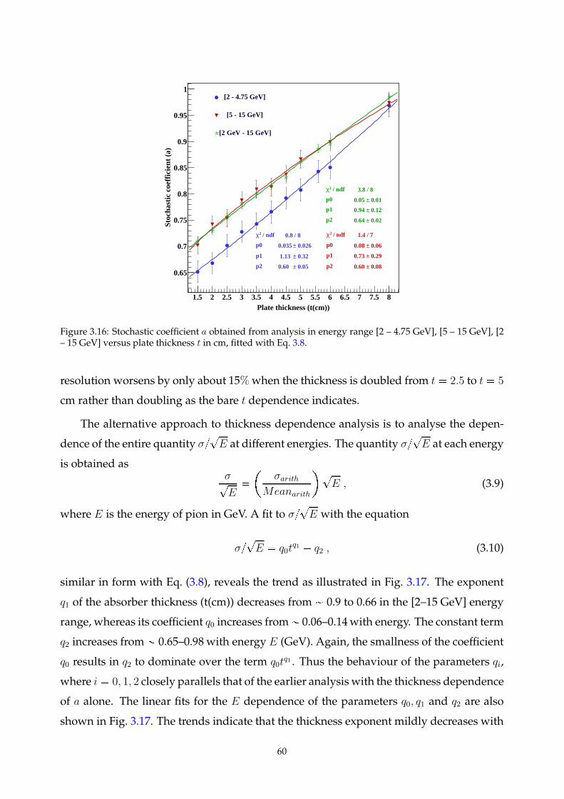
Plate thickness (t(cm))1.5 2 2.5 3 3.5 4 4.5 5 5.5 6 6.5 7 7.5 8

Sto

chas

tic c

oeffi

cien

t (a)

0.65

0.7

0.75

0.8

0.85

0.9

0.95

1

/ ndf 2χ 0.789 / 8

p0 0.02607± 0.03473

p1 0.3169± 1.13

p2 0.04741± 0.5987

/ ndf 2χ 0.8 / 8

p0 0.026± 0.035

p1 0.32± 1.13

p2 0.05± 0.60

/ ndf 2χ 1.401 / 7

p0 0.06436± 0.08097

p1 0.2866± 0.7337

p2 0.08471± 0.5993

/ ndf 2χ 1.4 / 7

p0 0.06± 0.08

p1 0.29± 0.73

p2 0.08± 0.60

/ ndf 2χ 3.8 / 8

p0 0.01± 0.05

p1 0.12± 0.94

p2 0.02± 0.6389

/ ndf 2χ 3.8 / 8

p0 0.01± 0.05

p1 0.12± 0.94

p2 0.02± 0.64

[2 - 4.75 GeV]

[5 - 15 GeV]

[2 GeV - 15 GeV]

Figure 3.16: Stochastic coefficient a obtained from analysis in energy range [2 – 4.75 GeV], [5 – 15 GeV], [2– 15 GeV] versus plate thickness t in cm, fitted with Eq. 3.8.

resolution worsens by only about 15%when the thickness is doubled from t 2.5 to t 5

cm rather than doubling as the bare t dependence indicates.

The alternative approach to thickness dependence analysis is to analyse the depen-

dence of the entire quantity σ?

E at different energies. The quantity σ?

E at each energy

is obtained asσ?

E

σarith

Meanarith

?

E , (3.9)

where E is the energy of pion in GeV. A fit to σ?

E with the equation

σ?

E q0tq1 q2 , (3.10)

similar in form with Eq. (3.8), reveals the trend as illustrated in Fig. 3.17. The exponent

q1 of the absorber thickness (t(cm)) decreases from 0.9 to 0.66 in the [2–15 GeV] energy

range, whereas its coefficient q0 increases from 0.06–0.14with energy. The constant term

q2 increases from 0.65–0.98 with energy E (GeV). Again, the smallness of the coefficient

q0 results in q2 to dominate over the term q0tq1 . Thus the behaviour of the parameters qi,

where i 0, 1, 2 closely parallels that of the earlier analysis with the thickness dependence

of a alone. The linear fits for the E dependence of the parameters q0, q1 and q2 are also

shown in Fig. 3.17. The trends indicate that the thickness exponent mildly decreases with

60

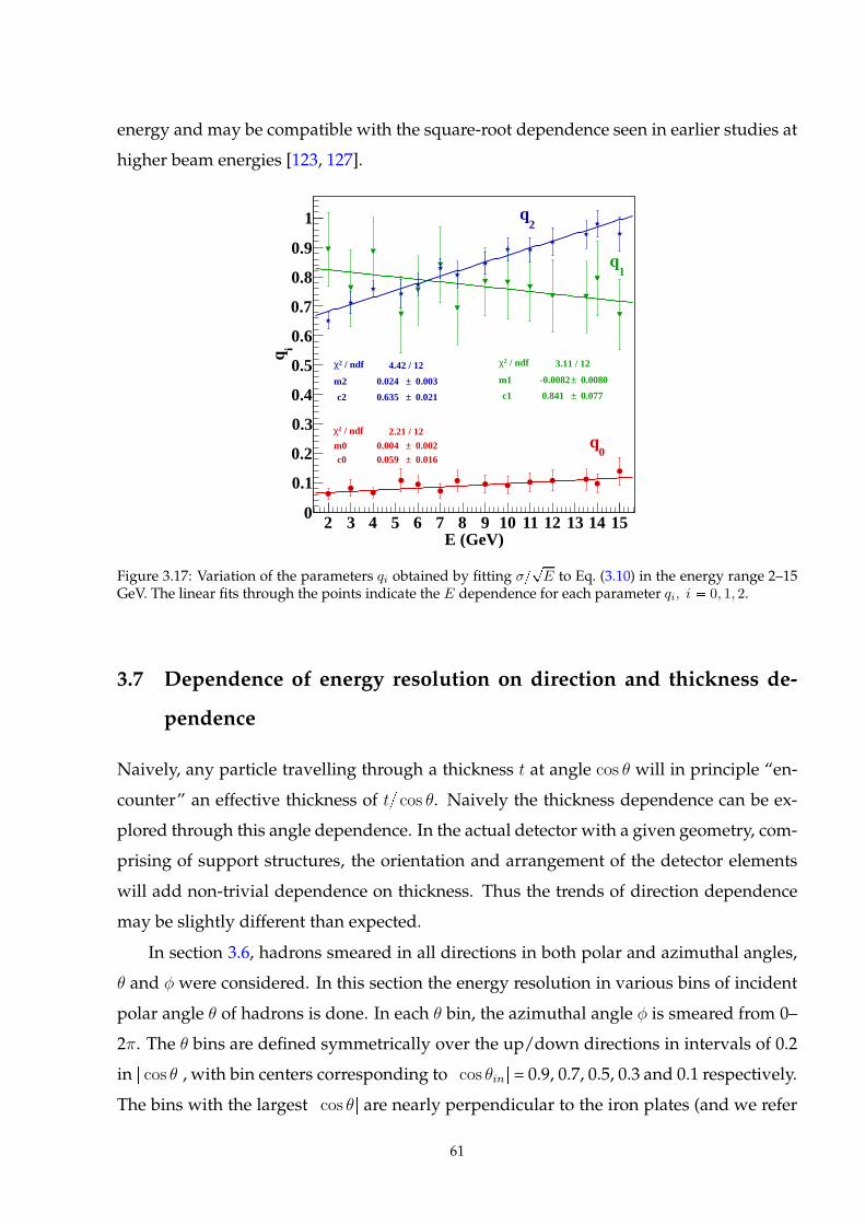
energy and may be compatible with the square-root dependence seen in earlier studies at

higher beam energies [123, 127].

E (GeV)2 3 4 5 6 7 8 9 10 11 12 13 14 15

iq

0

0.1

0.2

0.3

0.4

0.5

0.6

0.7

0.8

0.9

1

/ ndf 2χ 2.21 / 12m1 0.002± 0.004 c1 0.016± 0.059

/ ndf 2χ 2.21 / 12m0 0.002± 0.004 c0 0.016± 0.059

/ ndf 2χ 3.11 / 12

m2 0.0080± -0.0082

c2 0.077± 0.841

/ ndf 2χ 3.11 / 12

m1 0.0080± -0.0082

c1 0.077± 0.841

/ ndf 2χ 4.42 / 12

m3 0.003± 0.024

c3 0.021± 0.635

/ ndf 2χ 4.42 / 12

m2 0.003± 0.024

c2 0.021± 0.635

0q

1q

2q

Figure 3.17: Variation of the parameters qi obtained by fitting σ?

E to Eq. (3.10) in the energy range 2–15GeV. The linear fits through the points indicate the E dependence for each parameter qi, i 0, 1, 2.

3.7 Dependence of energy resolution on direction and thickness de-

pendence

Naively, any particle travelling through a thickness t at angle cos θ will in principle “en-

counter” an effective thickness of t cos θ. Naively the thickness dependence can be ex-

plored through this angle dependence. In the actual detector with a given geometry, com-

prising of support structures, the orientation and arrangement of the detector elements

will add non-trivial dependence on thickness. Thus the trends of direction dependence

may be slightly different than expected.

In section 3.6, hadrons smeared in all directions in both polar and azimuthal angles,

θ and φ were considered. In this section the energy resolution in various bins of incident

polar angle θ of hadrons is done. In each θ bin, the azimuthal angle φ is smeared from 0–

2π. The θ bins are defined symmetrically over the up/down directions in intervals of 0.2

in | cos θ|, with bin centers corresponding to | cos θin| = 0.9, 0.7, 0.5, 0.3 and 0.1 respectively.

The bins with the largest | cos θ| are nearly perpendicular to the iron plates (and we refer

61

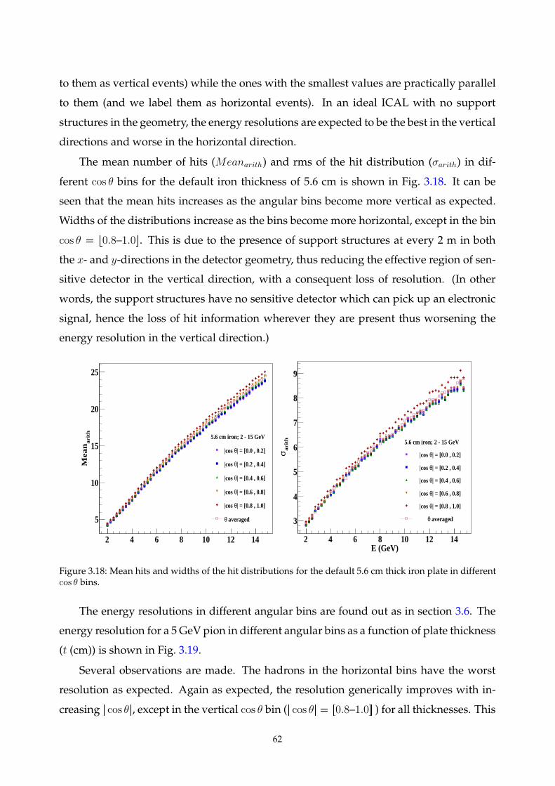
to them as vertical events) while the ones with the smallest values are practically parallel

to them (and we label them as horizontal events). In an ideal ICAL with no support

structures in the geometry, the energy resolutions are expected to be the best in the vertical

directions and worse in the horizontal direction.

The mean number of hits (Meanarith) and rms of the hit distribution (σarith) in dif-

ferent cos θ bins for the default iron thickness of 5.6 cm is shown in Fig. 3.18. It can be

seen that the mean hits increases as the angular bins become more vertical as expected.

Widths of the distributions increase as the bins become more horizontal, except in the bin

cos θ r0.8–1.0s. This is due to the presence of support structures at every 2 m in both

the x- and y-directions in the detector geometry, thus reducing the effective region of sen-

sitive detector in the vertical direction, with a consequent loss of resolution. (In other

words, the support structures have no sensitive detector which can pick up an electronic

signal, hence the loss of hit information wherever they are present thus worsening the

energy resolution in the vertical direction.)

2 4 6 8 10 12 14

arith

Me

an

5

10

15

20

25

5.6 cm iron; 2 - 15 GeV

| = [0.0 , 0.2]θ|cos

| = [0.2 , 0.4]θ|cos

| = [0.4 , 0.6]θ|cos

| = [0.6 , 0.8]θ|cos

| = [0.8 , 1.0]θ|cos

averagedθ

E (GeV)2 4 6 8 10 12 14

arith

σ

3

4

5

6

7

8

9

5.6 cm iron; 2 - 15 GeV

| = [0.0 , 0.2]θ|cos

| = [0.2 , 0.4]θ|cos

| = [0.4 , 0.6]θ|cos

| = [0.6 , 0.8]θ|cos

| = [0.8 , 1.0]θ|cos

averagedθ

Figure 3.18: Mean hits and widths of the hit distributions for the default 5.6 cm thick iron plate in differentcos θ bins.

The energy resolutions in different angular bins are found out as in section 3.6. The

energy resolution for a 5 GeV pion in different angular bins as a function of plate thickness

(t (cm)) is shown in Fig. 3.19.

Several observations are made. The hadrons in the horizontal bins have the worst

resolution as expected. Again as expected, the resolution generically improves with in-

creasing | cos θ|, except in the vertical cos θ bin (| cos θ| r0.8–1.0s ) for all thicknesses. This

62

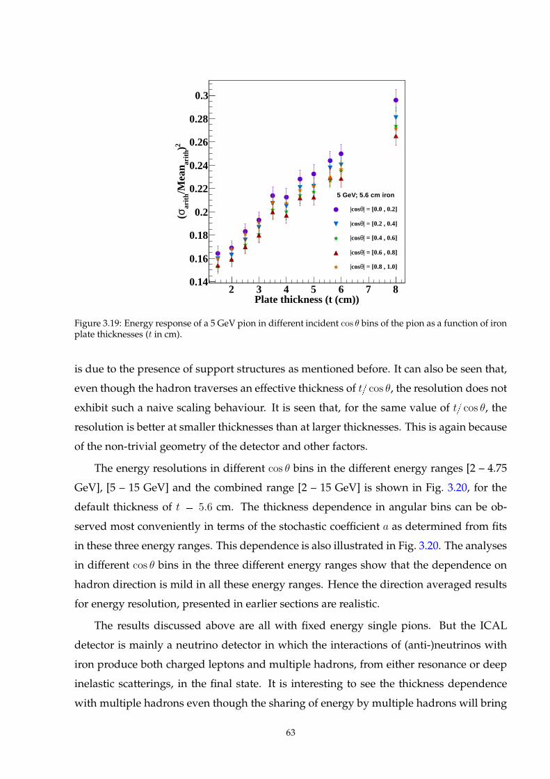
Plate thickness (t (cm))2 3 4 5 6 7 8

2 )ar

ith/M

ean

arith

σ(

0.14

0.16

0.18

0.2

0.22

0.24

0.26

0.28

0.3

5 GeV; 5.6 cm iron

| = [0.0 , 0.2]θ|cos

| = [0.2 , 0.4]θ|cos

| = [0.4 , 0.6]θ|cos

| = [0.6 , 0.8]θ|cos

| = [0.8 , 1.0]θ|cos

Figure 3.19: Energy response of a 5 GeV pion in different incident cos θ bins of the pion as a function of ironplate thicknesses (t in cm).

is due to the presence of support structures as mentioned before. It can also be seen that,

even though the hadron traverses an effective thickness of t cos θ, the resolution does not

exhibit such a naive scaling behaviour. It is seen that, for the same value of t cos θ, the

resolution is better at smaller thicknesses than at larger thicknesses. This is again because

of the non-trivial geometry of the detector and other factors.

The energy resolutions in different cos θ bins in the different energy ranges [2 – 4.75

GeV], [5 – 15 GeV] and the combined range [2 – 15 GeV] is shown in Fig. 3.20, for the

default thickness of t 5.6 cm. The thickness dependence in angular bins can be ob-

served most conveniently in terms of the stochastic coefficient a as determined from fits

in these three energy ranges. This dependence is also illustrated in Fig. 3.20. The analyses

in different cos θ bins in the three different energy ranges show that the dependence on

hadron direction is mild in all these energy ranges. Hence the direction averaged results

for energy resolution, presented in earlier sections are realistic.

The results discussed above are all with fixed energy single pions. But the ICAL

detector is mainly a neutrino detector in which the interactions of (anti-)neutrinos with

iron produce both charged leptons and multiple hadrons, from either resonance or deep

inelastic scatterings, in the final state. It is interesting to see the thickness dependence

with multiple hadrons even though the sharing of energy by multiple hadrons will bring

63

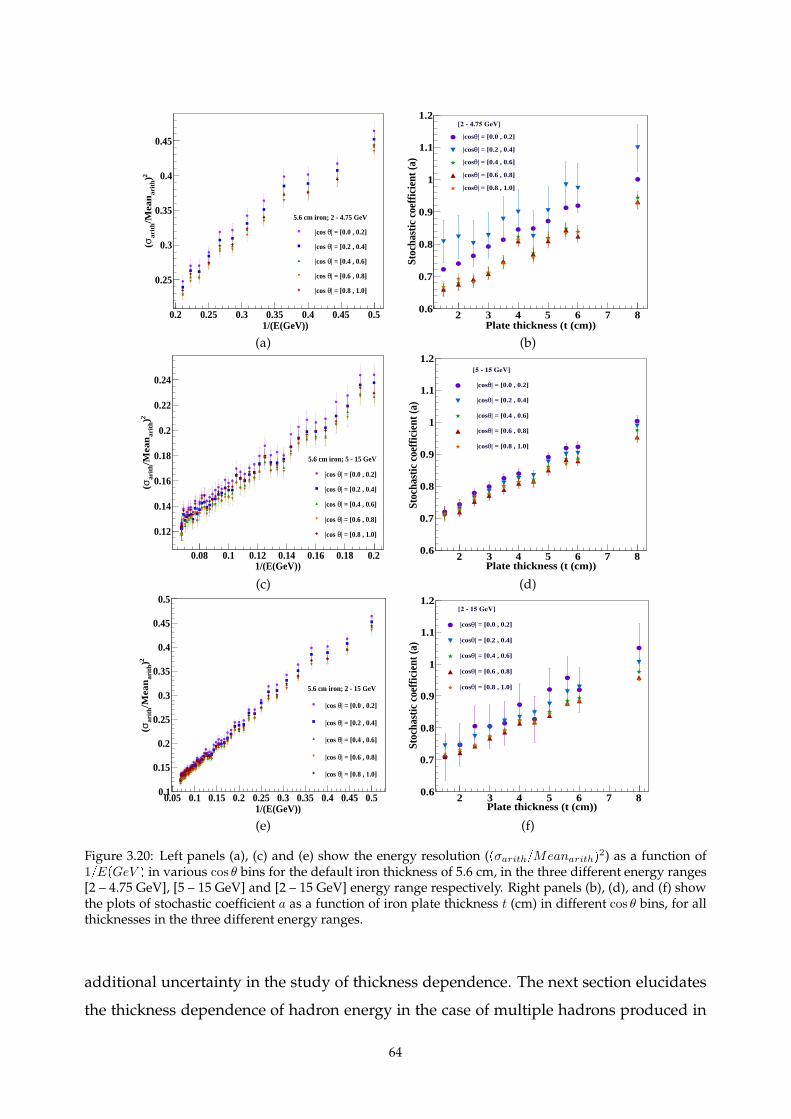
1/(E(GeV))0.2 0.25 0.3 0.35 0.4 0.45 0.5

2 )a

rith

/Me

an

arith

σ(

0.25

0.3

0.35

0.4

0.45

5.6 cm iron; 2 - 4.75 GeV

| = [0.0 , 0.2]θ|cos

| = [0.2 , 0.4]θ|cos

| = [0.4 , 0.6]θ|cos

| = [0.6 , 0.8]θ|cos

| = [0.8 , 1.0]θ|cos


Sto

chas

tic c

oeffi

cien

t (a)

0.6

0.7

0.8

0.9

1

1.1

1.2[2 4.75 GeV]

| = [0.0 , 0.2]θ|cos

| = [0.2 , 0.4]θ|cos

| = [0.4 , 0.6]θ|cos

| = [0.6 , 0.8]θ|cos

| = [0.8 , 1.0]θ|cos

(a) (b)

1/(E(GeV))0.08 0.1 0.12 0.14 0.16 0.18 0.2

2 )a

rith

/Me

an

arith

σ(

0.12

0.14

0.16

0.18

0.2

0.22

0.24

5.6 cm iron; 5 - 15 GeV

| = [0.0 , 0.2]θ|cos

| = [0.2 , 0.4]θ|cos

| = [0.4 , 0.6]θ|cos

| = [0.6 , 0.8]θ|cos

| = [0.8 , 1.0]θ|cos


Sto

chas

tic c

oeffi

cien

t (a)

0.6

0.7

0.8

0.9

1

1.1

1.2[5 15 GeV]

| = [0.0 , 0.2]θ|cos

| = [0.2 , 0.4]θ|cos

| = [0.4 , 0.6]θ|cos

| = [0.6 , 0.8]θ|cos

| = [0.8 , 1.0]θ|cos

(c) (d)

1/(E(GeV))0.05 0.1 0.15 0.2 0.25 0.3 0.35 0.4 0.45 0.5

2 )a

rith

/Me

an

arith

σ(

0.1

0.15

0.2

0.25

0.3

0.35

0.4

0.45

0.5

5.6 cm iron; 2 - 15 GeV

| = [0.0 , 0.2]θ|cos

| = [0.2 , 0.4]θ|cos

| = [0.4 , 0.6]θ|cos

| = [0.6 , 0.8]θ|cos

| = [0.8 , 1.0]θ|cos


Sto

chas

tic c

oeffi

cien

t (a)

0.6

0.7

0.8

0.9

1

1.1

1.2[2 15 GeV]

| = [0.0 , 0.2]θ|cos

| = [0.2 , 0.4]θ|cos

| = [0.4 , 0.6]θ|cos

| = [0.6 , 0.8]θ|cos

| = [0.8 , 1.0]θ|cos

(e) (f)

Figure 3.20: Left panels (a), (c) and (e) show the energy resolution (pσarithMeanarithq2) as a function of

1EpGeV q in various cos θ bins for the default iron thickness of 5.6 cm, in the three different energy ranges[2 – 4.75 GeV], [5 – 15 GeV] and [2 – 15 GeV] energy range respectively. Right panels (b), (d), and (f) showthe plots of stochastic coefficient a as a function of iron plate thickness t (cm) in different cos θ bins, for allthicknesses in the three different energy ranges.

additional uncertainty in the study of thickness dependence. The next section elucidates

the thickness dependence of hadron energy in the case of multiple hadrons produced in

64

neutrino interactions.

3.8 Study of thickness dependence of hadron energy resolution formul-

tiple hadrons produced in neutrino interactions

In the earlier study [20] for the fixed absorber thickness of t 5.6 cm, a comparison

of single pion resolutions with those of multiple hadrons generated in neutrino events

generated by NUANCE neutrino event generator was carried out [20]. This study is pre-

sented elsewhere. In the case of multiple hadrons there is a non-trivial partition of energy

between different hadronic final states. In this section, the thickness dependence of mul-

tiple hadrons for the direction averaged case is discussed. The trends in the thickness

dependence of the resolution quantified by pσEq2 and stochastic coefficient a are found

to be similar in both cases.

3.9 Effect of different hadron models on hadron energy resolution

The effect of different hadronisation models was investigated for the default iron thick-

ness of 5.6 cm. In this regard, the LHEP model used in GEANT4 was replaced [23]

with QGSP (for hadrons with energy ¡ 12 GeV) and QGSP BERT (for the lower energy

hadrons). The energy resolution was found to be reasonably model independent, with a

variation in the mean (rms) of less than 4% (5%) among different models in the energy

range from 2–15 GeV for t 5.6 cm.

3.10 Comparison of the simulation studies using ICAL with other ex-

periments

To validate the analysis presented above, the hadron resolutions from ICAL simulation

studies have been compared with simulations of both MONOLITH and MINOS collab-

orations and also to their test beam data. In the current simulation study ICAL with 8

cm iron plate has a resolution of 98.5%?

E ` 29.4%. This is roughly comparable to the

angle-averaged result of 90%?

E` 30% obtained from the simulation studies of MONO-

LITH [128] with the same iron plate thickness. For the convenience in comparing, the

convention a?

E ` b a

a2E b2 has been used.

65

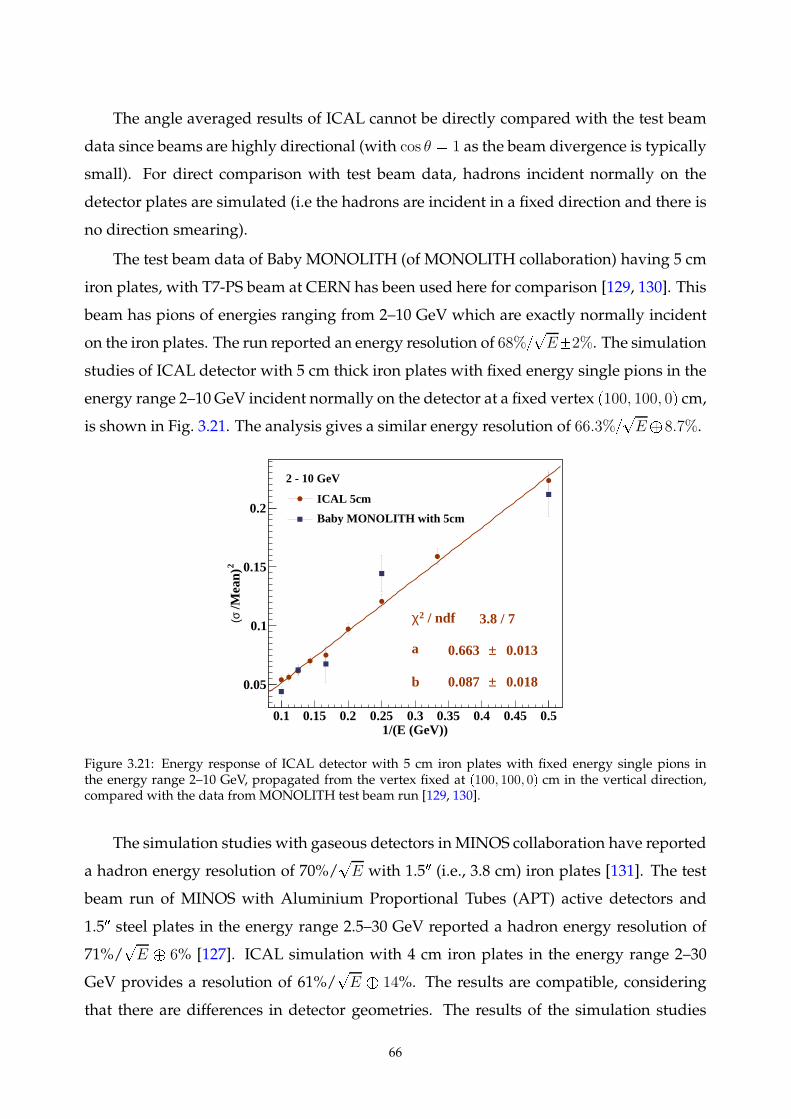
The angle averaged results of ICAL cannot be directly compared with the test beam

data since beams are highly directional (with cos θ 1 as the beam divergence is typically

small). For direct comparison with test beam data, hadrons incident normally on the

detector plates are simulated (i.e the hadrons are incident in a fixed direction and there is

no direction smearing).

The test beam data of Baby MONOLITH (of MONOLITH collaboration) having 5 cm

iron plates, with T7-PS beam at CERN has been used here for comparison [129, 130]. This

beam has pions of energies ranging from 2–10 GeV which are exactly normally incident

on the iron plates. The run reported an energy resolution of 68%?

E2%. The simulation

studies of ICAL detector with 5 cm thick iron plates with fixed energy single pions in the

energy range 2–10 GeV incident normally on the detector at a fixed vertex p100, 100, 0q cm,

is shown in Fig. 3.21. The analysis gives a similar energy resolution of 66.3%?

E` 8.7%.

1/(E (GeV))0.1 0.15 0.2 0.25 0.3 0.35 0.4 0.45 0.5

2/M

ean)

(σ

0.05

0.1

0.15

0.2

/ ndf 2χ 3.824 / 7

a 0.013± 0.663

b 0.02± 0.09

/ ndf 2χ 3.8 / 7

a 0.013± 0.663

b 0.018± 0.087

2 - 10 GeV

ICAL 5cm

Baby MONOLITH with 5cm

Figure 3.21: Energy response of ICAL detector with 5 cm iron plates with fixed energy single pions inthe energy range 2–10 GeV, propagated from the vertex fixed at p100, 100, 0q cm in the vertical direction,compared with the data fromMONOLITH test beam run [129, 130].

The simulation studies with gaseous detectors inMINOS collaboration have reported

a hadron energy resolution of 70%/?

E with 1.52 (i.e., 3.8 cm) iron plates [131]. The test

beam run of MINOS with Aluminium Proportional Tubes (APT) active detectors and

1.52 steel plates in the energy range 2.5–30 GeV reported a hadron energy resolution of

71%/?

E ` 6% [127]. ICAL simulation with 4 cm iron plates in the energy range 2–30

GeV provides a resolution of 61%/?

E ` 14%. The results are compatible, considering

that there are differences in detector geometries. The results of the simulation studies

66

with ICAL detector thus agree with those of MINOS and MONOLITH simulations and

test beam results within statistical errors. The slight differences in the resolutions can

be attributed to differences in the details of the detector configuration. it should be noted

that fixed vertex data tend to give smaller values of b than the smeared vertex case. This is

because the hadrons see more inhomogeneities in the detector geometry owing to the fact

that the vertices are spread over a region and hence the effects due to detector geometry

also come in. This is reflected in the larger residual resolution.

The study of hadron energy resolution is important owing to the fact that the in-

clusion of hadron energy information in the atmospheric neutrino oscillation analysis

enables the improvement in the precision measurements of θ23 and ∆m232 as well as af-

fecting the hierarchy determination. This will be discussed in detail in Chapter6. It is

equally important to determine the direction resolution of hadrons also, since this is the

determining piece in the reconstruction of neutrino direction. The following section elu-

cidates the determination of direction resolution of hadrons using hit information and

timing of those hits. However, this information has not been included in the physics

analysis in Chapter 6.

3.11 eh ratio in ICAL

Since the atmospheric neutrinos contain νµ and νe in the 2:1 ratio, there are charged cur-

rent electron neutrino interactions also in ICAL, which produce electrons in the final state

according to Table 3.1 to in Section 3.2. These electrons produce showers and hence can-

not be distinguished directly from hadrons in ICAL. The hadronic shower in ICAL also

contains an electromagnetic component since the neutral pions (π0) decay in two gam-

mas (γ) which then produce electromagnetic showers by pair production. Studying the

ratio of electron response to charged pion response, i.e, eh ratio helps the characterisa-

tion of the effect of neutral hadrons on hadron energy resolution. The hit distributions of

electrons, gammas and neutral pions are similar in ICAL. This is illustrated in Fig. 3.22,

where the hit distributions from electrons, gammas, and neutral pions at 5 GeV energy

are shown.

The simulation studies of eh ratio in ICAL have been conducted using fixed energy

single electrons and charged pions (π), 1,00,000 single particles, for each energy, gener-

ated in the energy range 2–15 GeV, with vertices randomised over a fiducial volume of 2

67

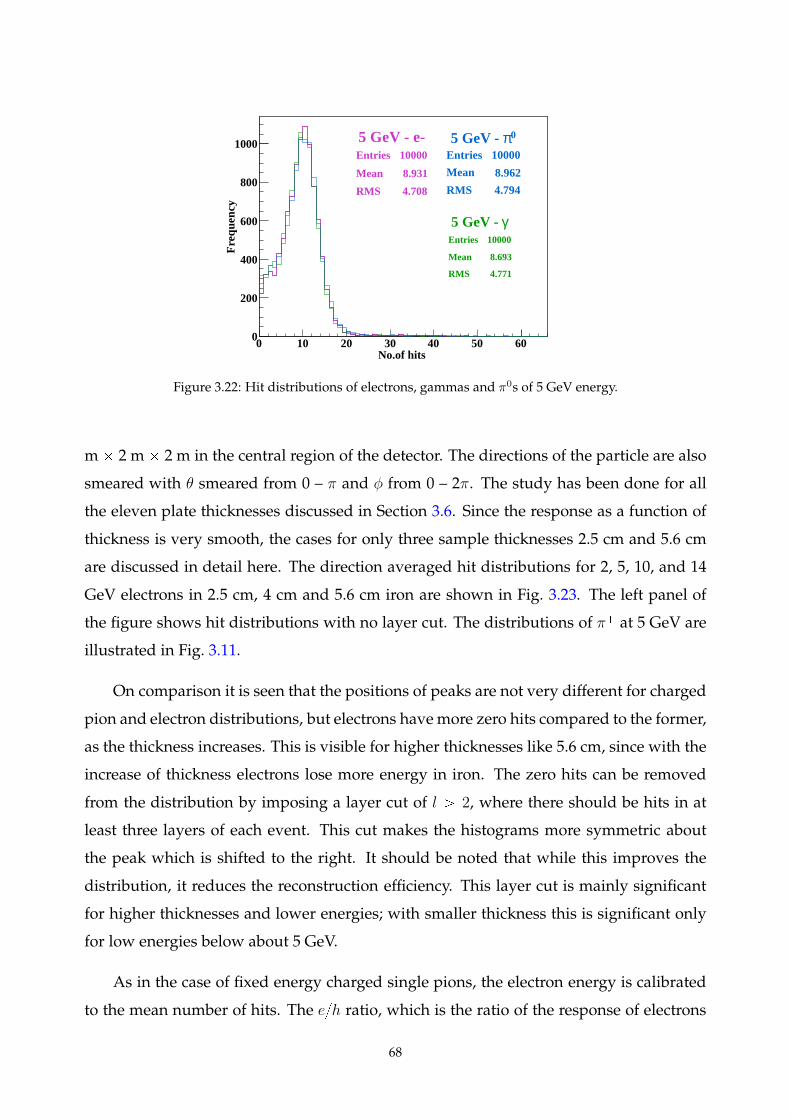
5 GeV - e-Entries 10000

Mean 8.931

RMS 4.708

No.of hits 0 10 20 30 40 50 60

Fre

quen

cy

0

200

400

600

800

1000 5 GeV - e-Entries 10000

Mean 8.931

RMS 4.708

htempEntries 10000Mean 8.931RMS 4.708

htempEntries 10000Mean 8.931RMS 4.708

0π5 GeV - Entries 10000

Mean 8.962

RMS 4.794

0π5 GeV - Entries 10000

Mean 8.962

RMS 4.794

γ5 GeV - Entries 10000

Mean 8.693

RMS 4.771

γ5 GeV - Entries 10000

Mean 8.693

RMS 4.771

Figure 3.22: Hit distributions of electrons, gammas and π0s of 5 GeV energy.

m 2 m 2 m in the central region of the detector. The directions of the particle are also

smeared with θ smeared from 0 – π and φ from 0 – 2π. The study has been done for all

the eleven plate thicknesses discussed in Section 3.6. Since the response as a function of

thickness is very smooth, the cases for only three sample thicknesses 2.5 cm and 5.6 cm

are discussed in detail here. The direction averaged hit distributions for 2, 5, 10, and 14

GeV electrons in 2.5 cm, 4 cm and 5.6 cm iron are shown in Fig. 3.23. The left panel of

the figure shows hit distributions with no layer cut. The distributions of π at 5 GeV are

illustrated in Fig. 3.11.

On comparison it is seen that the positions of peaks are not very different for charged

pion and electron distributions, but electrons havemore zero hits compared to the former,

as the thickness increases. This is visible for higher thicknesses like 5.6 cm, since with the

increase of thickness electrons lose more energy in iron. The zero hits can be removed

from the distribution by imposing a layer cut of l ¡ 2, where there should be hits in at

least three layers of each event. This cut makes the histograms more symmetric about

the peak which is shifted to the right. It should be noted that while this improves the

distribution, it reduces the reconstruction efficiency. This layer cut is mainly significant

for higher thicknesses and lower energies; with smaller thickness this is significant only

for low energies below about 5 GeV.

As in the case of fixed energy charged single pions, the electron energy is calibrated

to the mean number of hits. The eh ratio, which is the ratio of the response of electrons

68

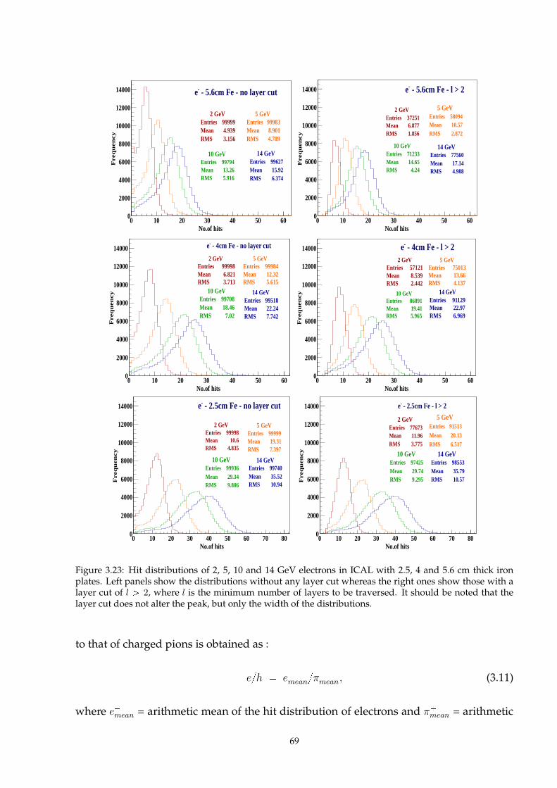
14 GeV Entries 99627Mean 15.92RMS 6.374

No.of hits 0 10 20 30 40 50 60

Fre

qu

en

cy

0

2000

4000

6000

8000

10000

12000

14000


- 5.6cm Fe - no layer cut-e








No.of hits 0 10 20 30 40 50 60

Fre

qu

en

cy

0

2000

4000

6000

8000

10000

12000

14000


- 5.6cm Fe - l > 2 -e








No.of hits 0 10 20 30 40 50 60

Fre

qu

en

cy

0

2000

4000

6000

8000

10000

12000

14000


- 4cm Fe - no layer cut-e








No.of hits0 10 20 30 40 50 60

Fre

qu

en

cy

0

2000

4000

6000

8000

10000

12000

14000


- 4cm Fe - l > 2 -e








No.of hits0 10 20 30 40 50 60 70 80

Fre

qu

en

cy

0

2000

4000

6000

8000

10000

12000

14000


- 2.5cm Fe - no layer cut-e








No.of hits 0 10 20 30 40 50 60 70 80

Fre

qu

en

cy

0

2000

4000

6000

8000

10000

12000

14000


- 2.5cm Fe - l > 2 -e







Figure 3.23: Hit distributions of 2, 5, 10 and 14 GeV electrons in ICAL with 2.5, 4 and 5.6 cm thick ironplates. Left panels show the distributions without any layer cut whereas the right ones show those with alayer cut of l ¡ 2, where l is the minimum number of layers to be traversed. It should be noted that thelayer cut does not alter the peak, but only the width of the distributions.

to that of charged pions is obtained as :

eh emeanπ

mean, (3.11)

where emean = arithmetic mean of the hit distribution of electrons and πmean = arithmetic

69

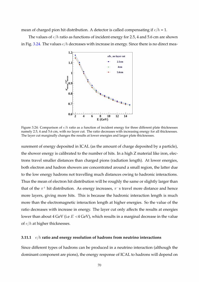
mean of charged pion hit distribution. A detector is called compensating if eh = 1.

The values of eh ratio as functions of incident energy for 2.5, 4 and 5.6 cm are shown

in Fig. 3.24. The values eh decreases with increase in energy. Since there is no direct mea-

E (GeV)2 4 6 8 10 12 14

mea

n+ π/

mea

n- e

0.6

0.7

0.8

0.9

1

1.1

1.2 e/h , no layer cut

2.5cm

4cm

5.6cm

Figure 3.24: Comparison of eh ratio as a function of incident energy for three different plate thicknessesnamely 2.5, 4 and 5.6 cm, with no layer cut. The ratio decreases with increasing energy for all thicknesses.The layer cut marginally changes the results at lower energies and larger plate thicknesses.

surement of energy deposited in ICAL (as the amount of charge deposited by a particle),

the shower energy is calibrated to the number of hits. In a high Z material like iron, elec-

trons travel smaller distances than charged pions (radiation length). At lower energies,

both electron and hadron showers are concentrated around a small region, the latter due

to the low energy hadrons not travelling much distances owing to hadronic interactions.

Thus the mean of electron hit distribution will be roughly the same or slightly larger than

that of the π hit distribution. As energy increases, πs travel more distance and hence

more layers, giving more hits. This is because the hadronic interaction length is much

more than the electromagnetic interaction length at higher energies. So the value of the

ratio decreases with increase in energy. The layer cut only affects the results at energies

lower than about 4 GeV (i.e E 4 GeV), which results in a marginal decrease in the value

of eh at higher thicknesses.

3.11.1 eh ratio and energy resolution of hadrons from neutrino interactions

Since different types of hadrons can be produced in a neutrino interaction (although the

dominant component are pions), the energy response of ICAL to hadrons will depend on

70

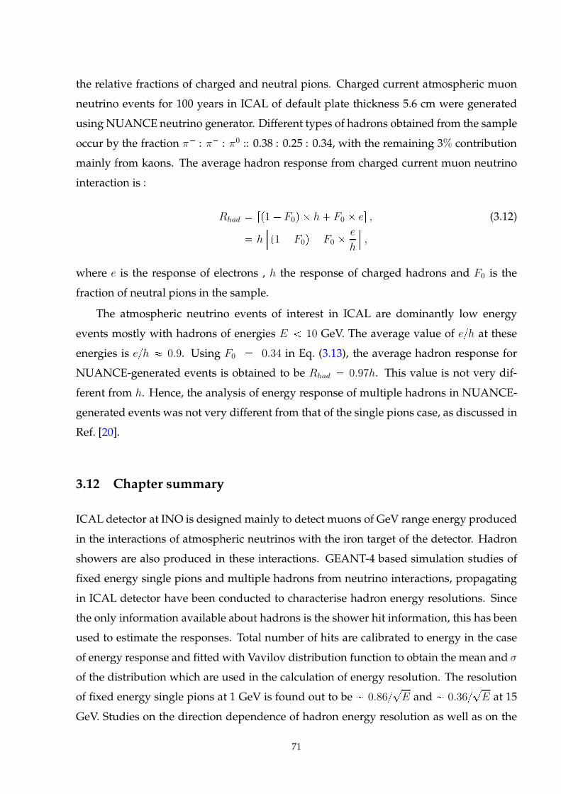
the relative fractions of charged and neutral pions. Charged current atmospheric muon

neutrino events for 100 years in ICAL of default plate thickness 5.6 cm were generated

using NUANCE neutrino generator. Different types of hadrons obtained from the sample

occur by the fraction π : π : π0 :: 0.38 : 0.25 : 0.34, with the remaining 3% contribution

mainly from kaons. The average hadron response from charged current muon neutrino

interaction is :

Rhad rp1 F0q h F0 es , (3.12)

h

p1 F0q F0

e

h

,

where e is the response of electrons , h the response of charged hadrons and F0 is the

fraction of neutral pions in the sample.

The atmospheric neutrino events of interest in ICAL are dominantly low energy

events mostly with hadrons of energies E 10 GeV. The average value of eh at these

energies is eh 0.9. Using F0 0.34 in Eq. (3.13), the average hadron response for

NUANCE-generated events is obtained to be Rhad 0.97h. This value is not very dif-

ferent from h. Hence, the analysis of energy response of multiple hadrons in NUANCE-

generated events was not very different from that of the single pions case, as discussed in

Ref. [20].

3.12 Chapter summary

ICAL detector at INO is designed mainly to detect muons of GeV range energy produced

in the interactions of atmospheric neutrinos with the iron target of the detector. Hadron

showers are also produced in these interactions. GEANT-4 based simulation studies of

fixed energy single pions and multiple hadrons from neutrino interactions, propagating

in ICAL detector have been conducted to characterise hadron energy resolutions. Since

the only information available about hadrons is the shower hit information, this has been

used to estimate the responses. Total number of hits are calibrated to energy in the case

of energy response and fitted with Vavilov distribution function to obtain the mean and σ

of the distribution which are used in the calculation of energy resolution. The resolution

of fixed energy single pions at 1 GeV is found out to be 0.86?

E and 0.36?

E at 15

GeV. Studies on the direction dependence of hadron energy resolution as well as on the

71

thickness of iron plate have also been conducted.

This study is relevant in the context of physics potential of ICAL, since the inclusion

of hadron energy as an observable in the oscillation analysis improves ICAL sensitivities

[27]. Thus the effect of plate thickness is crucial for both hadron and muon energies

since any improvement in their resolutions will further better ICAL results. The study

shows that the dependence on thickness is not a trivial?

t one but is mostly driven by

a ”residual resolution“ which is due to the intrinsic uncertainties of strong interactions,

fluctuations and detector geometry, which means that there will be a finite uncertainty

in the measurement of hadron energy even if the thickness is reduced to infinitesimally

small values. The study also shows that due to the presence of support structures in

the vertical direction corresponding to the cos θ 0.9 0.1 bin, the resolution in this

direction is not the best one as expected. The comparison of ICAL simulations with the

simulations of MONOLITH andMINOS and their test beam runs are found tomatch. The

ratio of electron response to pion response, i.e., the eh ratio has been calculated and used

to cross check the resolutions of multiple hadrons produced in neutrino interactions.

72

4Simulation studies of direction reso-

lution of hadrons in ICAL

4.1 Overview

As mentioned in Chapter 3, the energy and direction of the hadrons in the final state of

a neutrino interaction have to be reconstructed in order to reconsrtuct the energy and di-

rection of the interacting neutrino. Since the only information available about hadrons

in ICAL is the shower hit information, it has to be utilised to determine the energy and

direction resolutions of hadrons in ICAL. The detailed description of how to use the num-

ber of hits in the shower to determine the energy resolution of hadrons was presented in

Chapter 3. This chapter describes the simulation studies on how to use the position and

timing information of the hadron hits to reconstruct the shower direction. A method

called “raw hit” method which makes use of only the position and timing of hadron hits

is used to reconstruct the direction of hadrons. The studies on the resolution of the open-

ing angle between the muon and hadron shower in charged current muon neutrino and

anti-neutrino interactions are also discussed in detail. The work reported in this chapter

forms a part of Ref.[28].

4.2 Direction resolution of hadrons using hit and timing information

of the hits (the raw hit method)

As discussed in previous sections, hadrons only leave showers in the detector. Since the

only information available on hadrons are their hit positions and timings, in ICAL, these

have to be made use of in the reconstruction of the hadron shower direction. Again as

in the case of energy resolution, the hit information is used, but with the difference that

they are not counted, but their actual positions and timing are used to reconstruct the

hadron shower. This method is called the Raw Hit Method (RHM). This method has

the advantage that it can be used in the reconstruction of direction of hadrons produced

in both charged current and neutral current interactions, since it doesn’t require a vertex

with respect to which the direction can be reconstructed. The simulation studieswith both

fixed energy single pions and multiple hadrons from atmospheric neutrino interactions

generated using NUANCE neutrino generator have been conducted for the default iron

plate thickness of 5.6 cm. (Hadron direction resolution studies have been conducted only

using 5.6 cm.) The reconstruction of hadron direction is discussed in detail below.

4.2.1 Raw hit method (RHM)

The real advantage of this method is that it can be used in the reconstruction of the direc-

tion of hadrons produced in both charged current and neutral current interactions. There

is no need for a vertex (especially a charged lepton vertex) with respect to which the di-

rection can be reconstructed. Only the hit information in the X Z and Y Z planes

and the timings of the hits are required for direction reconstruction. Analysing the hits

separately in two different planes eliminates the problem of ghost hits by double counting

of hits taken in 3-D. This problem arises because of the large multiplicity of hits per layer

with hadrons in contrast to the minimum ionising muon. The problem is exacerbated

with multiple hadrons as obtained in a realisitic neutrino interaction. Since X and Y

hit information are obtained from different (upper and lower) strips in a layer (Z), it is

not obvious which X and Y are to be paired to give px, y, zq information. Allowing

for all possible combinations gives rise to spurious hits in that layer, these are ghost hits.

Timing information is crucial in telling if the hadron is traveling UP or DOWN.

To avoid the ghost-hits problem, the analysis was done separately in both X-Z and

Y-Z planes. The true hits are separated out first. While doing this, only hits within a time

window of ¤ 51 ns in a layer are selected. This is done to avoid taking into account hits

which are far away in time hits separated by upto 2.2µs (the muon life time may be seen

in a layer) and make sure that the hits are actually due to a single interaction.

The x - positions in a single layer are averaged to get the mean x - position in that

layer. i.e.,

xrisaverage xr1s xr2s ...xrnhitss

nhitsris, (4.1)

where xrisaverage is the average x position in the ith layer of an event (position in cm ;

obtained from the hit output from ICAL code). Similarly

yrisaverage yr1s yr2s ...yrnhitss

nhitsris, (4.2)

74

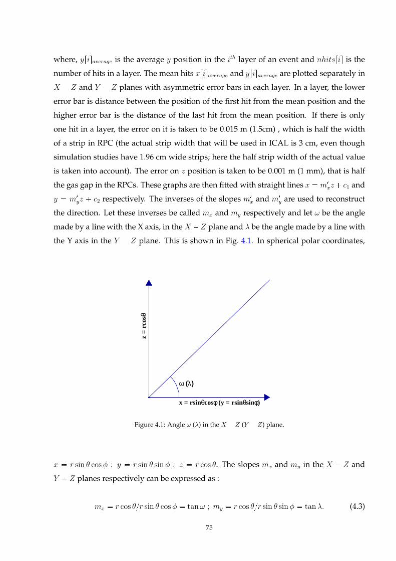
where, yrisaverage is the average y position in the ith layer of an event and nhitsris is the

number of hits in a layer. The mean hits xrisaverage and yrisaverage are plotted separately in

X Z and Y Z planes with asymmetric error bars in each layer. In a layer, the lower

error bar is distance between the position of the first hit from the mean position and the

higher error bar is the distance of the last hit from the mean position. If there is only

one hit in a layer, the error on it is taken to be 0.015 m (1.5cm) , which is half the width

of a strip in RPC (the actual strip width that will be used in ICAL is 3 cm, even though

simulation studies have 1.96 cm wide strips; here the half strip width of the actual value

is taken into account). The error on z position is taken to be 0.001 m (1 mm), that is half

the gas gap in the RPCs. These graphs are then fitted with straight lines x m1

xz c1 and

y m1

yz c2 respectively. The inverses of the slopes m1

x and m1

y are used to reconstruct

the direction. Let these inverses be called mx and my respectively and let ω be the angle

made by a line with the X axis, in theX Z plane and λ be the angle made by a line with

the Y axis in the Y Z plane. This is shown in Fig. 4.1. In spherical polar coordinates,

)φsinθ (y = rsinφcosθx = rsin

θz

= r

cos

)λ (ω

Figure 4.1: Angle ω (λ) in the X Z (Y Z) plane.

x r sin θ cosφ ; y r sin θ sinφ ; z r cos θ. The slopes mx and my in the X Z and

Y Z planes respectively can be expressed as :

mx r cos θr sin θ cosφ tanω ; my r cos θr sin θ sin φ tanλ. (4.3)

75

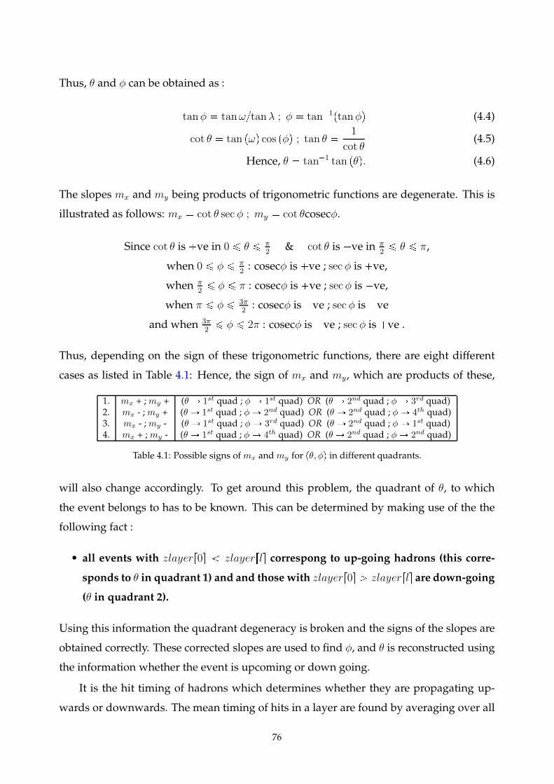
Thus, θ and φ can be obtained as :

tanφ tanωtanλ ; φ tan1ptanφq (4.4)

cot θ tan pωq cos pφq ; tan θ 1

cot θ(4.5)

Hence, θ tan1 tan pθq. (4.6)

The slopes mx and my being products of trigonometric functions are degenerate. This is

illustrated as follows: mx cot θ sec φ ; my cot θcosecφ.

Since cot θ is ve in 0 ¤ θ ¤ π2

& cot θ is ve in π2¤ θ ¤ π,

when 0 ¤ φ ¤ π2: cosecφ is ve ; sec φ is ve,

when π2¤ φ ¤ π : cosecφ is ve ; secφ is ve,

when π ¤ φ ¤ 3π2: cosecφ is ve ; secφ is ve

and when 3π2¤ φ ¤ 2π : cosecφ is ve ; sec φ is ve .

Thus, depending on the sign of these trigonometric functions, there are eight different

cases as listed in Table 4.1: Hence, the sign of mx and my, which are products of these,

1. mx + ;my + (θ Ñ 1st quad ; φÑ 1st quad) OR (θ Ñ 2nd quad ; φÑ 3rd quad)2. mx - ; my + (θ Ñ 1st quad ; φÑ 2nd quad) OR (θ Ñ 2nd quad ; φÑ 4th quad)3. mx - ;my - (θ Ñ 1st quad ; φÑ 3rd quad) OR (θ Ñ 2nd quad ; φÑ 1st quad)4. mx + ; my - (θ Ñ 1st quad ; φÑ 4th quad) OR (θ Ñ 2nd quad ; φÑ 2nd quad)

Table 4.1: Possible signs ofmx andmy for pθ, φq in different quadrants.

will also change accordingly. To get around this problem, the quadrant of θ, to which

the event belongs to has to be known. This can be determined by making use of the the

following fact :

• all events with zlayerr0s zlayerrls correspong to up-going hadrons (this corre-

sponds to θ in quadrant 1) and and those with zlayerr0s ¡ zlayerrls are down-going

(θ in quadrant 2).

Using this information the quadrant degeneracy is broken and the signs of the slopes are

obtained correctly. These corrected slopes are used to find φ, and θ is reconstructed using

the information whether the event is upcoming or down going.

It is the hit timing of hadrons which determines whether they are propagating up-

wards or downwards. The mean timing of hits in a layer are found by averaging over all

76

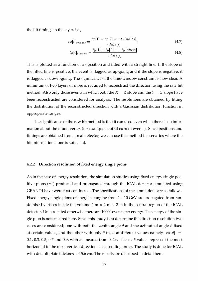
the hit timings in the layer. i.e.,

txrisaverage txr1s txr2s ...txrnhitss

nhitsris; (4.7)

tyrisaverage tyr1s tyr2s ...tyrnhitss

nhitsris. (4.8)

This is plotted as a function of z - position and fitted with a straight line. If the slope of

the fitted line is positive, the event is flagged as up-going and if the slope is negative, it

is flagged as down-going. The significance of the time-window constraint is now clear. A

minimum of two layers or more is required to reconstruct the direction using the raw hit

method. Also only those events in which both the X Z slope and the Y Z slope have

been reconstructed are considered for analysis. The resolutions are obtained by fitting

the distribution of the reconstructed direction with a Gaussian distribution function in

appropriate ranges.

The significance of the raw hit method is that it can used even when there is no infor-

mation about the muon vertex (for example neutral current events). Since positions and

timings are obtained from a real detector, we can use this method in scenarios where the

hit information alone is sufficient.

4.2.2 Direction resolution of fixed energy single pions

As in the case of energy resolution, the simulation studies using fixed energy single pos-

itive pions (π) produced and propagated through the ICAL detector simulated using

GEANT4 have were first conducted. The specifications of the simulations are as follows.

Fixed energy single pions of energies ranging from 1 – 10 GeV are propagated from ran-

domised vertices inside the volume 2 m 2 m 2 m in the central region of the ICAL

detector. Unless stated otherwise there are 10000 events per energy. The energy of the sin-

gle pion is not smeared here. Since this study is to determine the direction resolution two

cases are considered; one with both the zenith angle θ and the azimuthal angle φ fixed

at certain values, and the other with only θ fixed at different values namely | cos θ|

0.1, 0.3, 0.5, 0.7 and 0.9, with φ smeared from 0–2π. The cos θ values represent the most

horizontal to the most vertical directions in ascending order. The study is done for ICAL

with default plate thickness of 5.6 cm. The results are discussed in detail here.

77

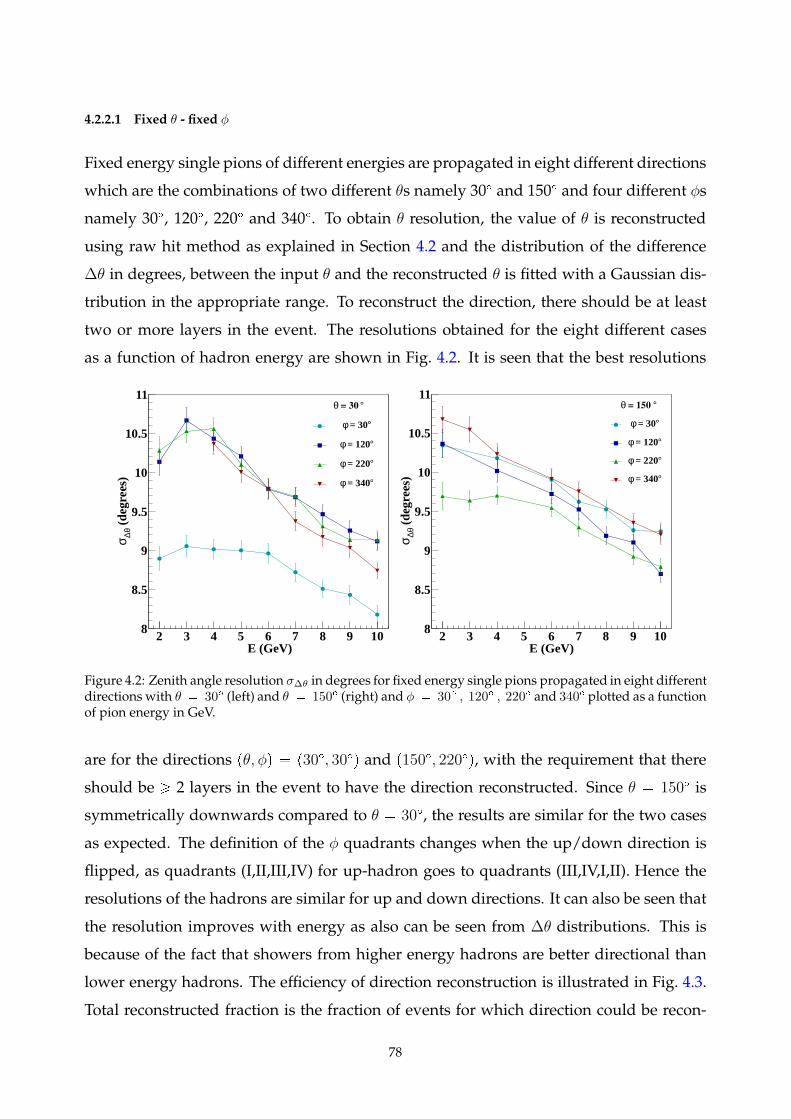
4.2.2.1 Fixed θ - fixed φ

Fixed energy single pions of different energies are propagated in eight different directions

which are the combinations of two different θs namely 30 and 150 and four different φs

namely 30, 120, 220 and 340. To obtain θ resolution, the value of θ is reconstructed

using raw hit method as explained in Section 4.2 and the distribution of the difference

∆θ in degrees, between the input θ and the reconstructed θ is fitted with a Gaussian dis-

tribution in the appropriate range. To reconstruct the direction, there should be at least

two or more layers in the event. The resolutions obtained for the eight different cases

as a function of hadron energy are shown in Fig. 4.2. It is seen that the best resolutions

E (GeV)2 3 4 5 6 7 8 9 10

(de

gree

s)θ∆σ

8

8.5

9

9.5

10

10.5

11° = 30θ

° = 30φ

° = 120φ

° = 220φ

° = 340φ

E (GeV)2 3 4 5 6 7 8 9 10

(de

gree

s)θ∆σ

8

8.5

9

9.5

10

10.5

11° = 150θ

° = 30φ

° = 120φ

° = 220φ

° = 340φ

Figure 4.2: Zenith angle resolution σ∆θ in degrees for fixed energy single pions propagated in eight differentdirections with θ 30 (left) and θ 150 (right) and φ 30 , 120 , 220 and 340 plotted as a functionof pion energy in GeV.

are for the directions pθ, φq p30, 30q and p150, 220q, with the requirement that there

should be ¥ 2 layers in the event to have the direction reconstructed. Since θ 150 is

symmetrically downwards compared to θ 30, the results are similar for the two cases

as expected. The definition of the φ quadrants changes when the up/down direction is

flipped, as quadrants (I,II,III,IV) for up-hadron goes to quadrants (III,IV,I,II). Hence the

resolutions of the hadrons are similar for up and down directions. It can also be seen that

the resolution improves with energy as also can be seen from ∆θ distributions. This is

because of the fact that showers from higher energy hadrons are better directional than

lower energy hadrons. The efficiency of direction reconstruction is illustrated in Fig. 4.3.

Total reconstructed fraction is the fraction of events for which direction could be recon-

78

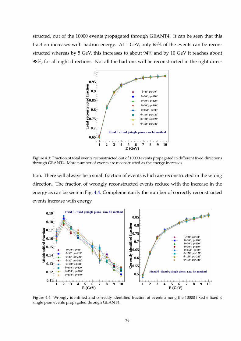
structed, out of the 10000 events propagated through GEANT4. It can be seen that this

fraction increases with hadron energy. At 1 GeV, only 65% of the events can be recon-

structed whereas by 5 GeV, this increases to about 94% and by 10 GeV it reaches about

98%, for all eight directions. Not all the hadrons will be reconstructed in the right direc-

E (GeV)1 2 3 4 5 6 7 8 9 10

Tota

l rec

onst

ruct

ed fr

actio

n

0.65

0.7

0.75

0.8

0.85

0.9

0.95

1

°=30φ ; °=30θ

°=120φ ; °=30θ

°=220φ ; °=30θ

°=340φ ; °=30θ

°=30φ ; °=150θ

°=120φ ; °=150θ

°=220φ ; °=150θ

°=340φ ; °=150θ

single pions, raw hit method φ - fixed θFixed

Figure 4.3: Fraction of total events reconstructed out of 10000 events propagated in different fixed directionsthrough GEANT4. More number of events are reconstructed as the energy increases.

tion. There will always be a small fraction of events which are reconstructed in the wrong

direction. The fraction of wrongly reconstructed events reduce with the increase in the

energy as can be seen in Fig. 4.4. Complementarily the number of correctly reconstructed

events increase with energy.

E (GeV)1 2 3 4 5 6 7 8 9 10

Mis

iden

tifie

d fr

actio

n

0.11

0.12

0.13

0.14

0.15

0.16

0.17

0.18

0.19

°=30φ ; °=30θ°=120φ ; °=30θ°=220φ ; °=30θ°=340φ ; °=30θ°=30φ ; °=150θ°=120φ ; °=150θ°=220φ ; °=150θ°=340φ ; °=150θ

single pions , raw hit method φ - fixed θFixed

E (GeV)1 2 3 4 5 6 7 8 9 10

Cor

rect

ly id

entif

ied

frac

tion

0.5

0.55

0.6

0.65

0.7

0.75

0.8

0.85

°=30φ ; °=30θ°=120φ ; °=30θ°=220φ ; °=30θ°=340φ ; °=30θ°=30φ ; °=150θ°=120φ ; °=150θ°=220φ ; °=150θ°=340φ ; °=150θ

single pions, raw hit method φ - fixed θFixed

Figure 4.4: Wrongly identified and correctly identified fraction of events among the 10000 fixed θ fixed φ

single pion events propagated through GEANT4.

79

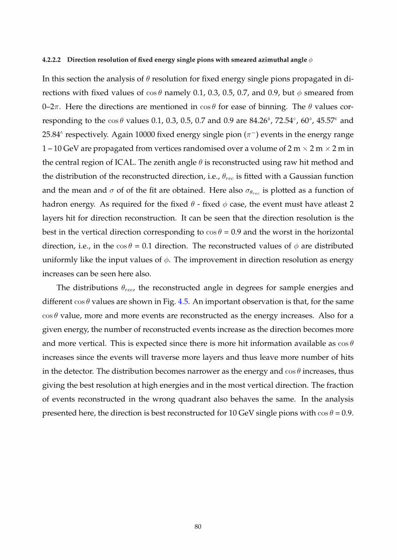
4.2.2.2 Direction resolution of fixed energy single pions with smeared azimuthal angle φ

In this section the analysis of θ resolution for fixed energy single pions propagated in di-

rections with fixed values of cos θ namely 0.1, 0.3, 0.5, 0.7, and 0.9, but φ smeared from

0–2π. Here the directions are mentioned in cos θ for ease of binning. The θ values cor-

responding to the cos θ values 0.1, 0.3, 0.5, 0.7 and 0.9 are 84.26, 72.54, 60, 45.57 and

25.84 respectively. Again 10000 fixed energy single pion (π) events in the energy range

1 – 10 GeV are propagated from vertices randomised over a volume of 2 m 2 m 2 m in

the central region of ICAL. The zenith angle θ is reconstructed using raw hit method and

the distribution of the reconstructed direction, i.e., θrec is fitted with a Gaussian function

and the mean and σ of of the fit are obtained. Here also σθrec is plotted as a function of

hadron energy. As required for the fixed θ - fixed φ case, the event must have atleast 2

layers hit for direction reconstruction. It can be seen that the direction resolution is the

best in the vertical direction corresponding to cos θ = 0.9 and the worst in the horizontal

direction, i.e., in the cos θ = 0.1 direction. The reconstructed values of φ are distributed

uniformly like the input values of φ. The improvement in direction resolution as energy

increases can be seen here also.

The distributions θrec, the reconstructed angle in degrees for sample energies and

different cos θ values are shown in Fig. 4.5. An important observation is that, for the same

cos θ value, more and more events are reconstructed as the energy increases. Also for a

given energy, the number of reconstructed events increase as the direction becomes more

and more vertical. This is expected since there is more hit information available as cos θ

increases since the events will traverse more layers and thus leave more number of hits

in the detector. The distribution becomes narrower as the energy and cos θ increases, thus

giving the best resolution at high energies and in the most vertical direction. The fraction

of events reconstructed in the wrong quadrant also behaves the same. In the analysis

presented here, the direction is best reconstructed for 10 GeV single pions with cos θ = 0.9.

80

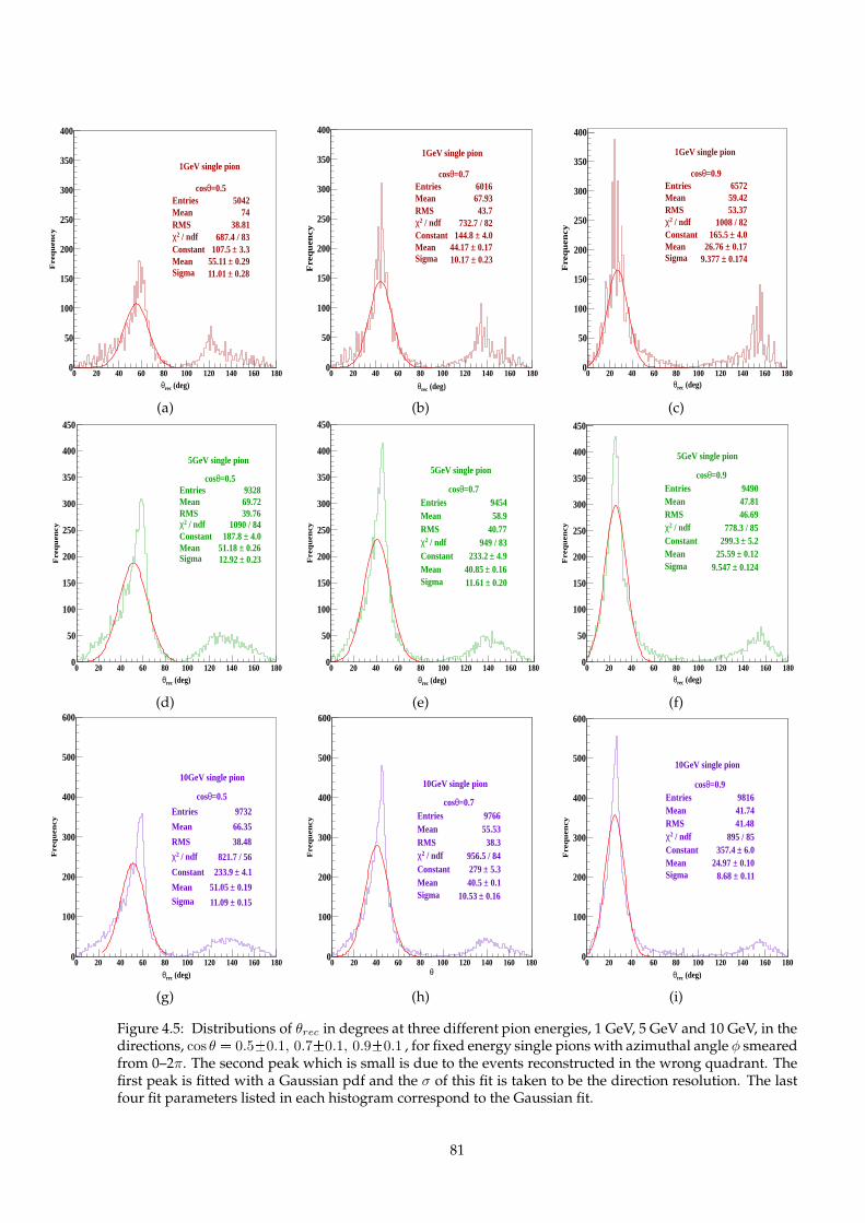
=0.5θcosEntries 5042Mean 74RMS 38.81

/ ndf 2χ 687.4 / 83Constant 3.3± 107.5 Mean 0.29± 55.11 Sigma 0.28± 11.01

(deg)recθ0 20 40 60 80 100 120 140 160 180

Fre

qu

en

cy

0

50

100

150

200

250

300

350

400

=0.5θcosEntries 5042Mean 74RMS 38.81


1GeV single pion=0.7θcos



(deg)recθ0 20 40 60 80 100 120 140 160 180

Fre

qu

en

cy

0

50

100

150

200

250

300

350

400

=0.7θcosEntries 6016Mean 67.93RMS 43.7


1GeV single pion


/ ndf 2χ 1008 / 82Constant 4.0± 165.5 Mean 0.17± 26.76 Sigma 0.174± 9.377

(deg)recθ0 20 40 60 80 100 120 140 160 180

Fre

qu

en

cy

0

50

100

150

200

250

300

350

400



1GeV single pion

(a) (b) (c)



(deg)recθ0 20 40 60 80 100 120 140 160 180

Fre

qu

en

cy

0

50

100

150

200

250

300

350

400

450



5GeV single pion



(deg)recθ0 20 40 60 80 100 120 140 160 180

Fre

qu

en

cy

0

50

100

150

200

250

300

350

400

450



5GeV single pion =0.9θcosEntries 9490Mean 47.81RMS 46.69


(deg)recθ0 20 40 60 80 100 120 140 160 180

Fre

qu

en

cy

0

50

100

150

200

250

300

350

400

450



5GeV single pion

(d) (e) (f)

=0.5θcos

Entries 9732

Mean 66.35

RMS 38.48

/ ndf 2χ 821.7 / 56

Constant 4.1± 233.9

Mean 0.19± 51.05 Sigma 0.15± 11.09

(deg)recθ0 20 40 60 80 100 120 140 160 180

Fre

qu

en

cy

0

100

200

300

400

500

600

=0.5θcos

Entries 9732

Mean 66.35

RMS 38.48

/ ndf 2χ 821.7 / 56


Mean 0.19± 51.05 Sigma 0.15± 11.09

10GeV single pion



θ0 20 40 60 80 100 120 140 160 180

Fre

qu

en

cy

0

100

200

300

400

500

600



10GeV single pion =0.9θcosEntries 9816Mean 41.74RMS 41.48


(deg)recθ0 20 40 60 80 100 120 140 160 180

Fre

qu

en

cy

0

100

200

300

400

500

600



10GeV single pion

(g) (h) (i)

Figure 4.5: Distributions of θrec in degrees at three different pion energies, 1 GeV, 5 GeV and 10 GeV, in thedirections, cos θ 0.50.1, 0.70.1, 0.90.1 , for fixed energy single pions with azimuthal angle φ smearedfrom 0–2π. The second peak which is small is due to the events reconstructed in the wrong quadrant. Thefirst peak is fitted with a Gaussian pdf and the σ of this fit is taken to be the direction resolution. The lastfour fit parameters listed in each histogram correspond to the Gaussian fit.

81

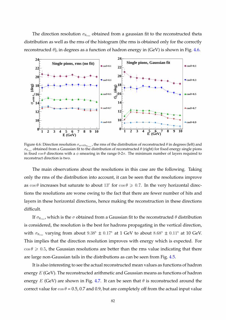
The direction resolution σθrec obtained from a gaussian fit to the reconstructed theta

distribution as well as the rms of the histogram (the rms is obtained only for the correctly

reconstructed θ), in degrees as a function of hadron energy in (GeV) is shown in Fig. 4.6.

E (GeV)1 2 3 4 5 6 7 8 9 10

(de

g)re

cθ

arith

σ

8

10

12

14

16

18

20

22

24

=0.1θcos

=0.3θcos

=0.5θcos

=0.7θcos

=0.9θcos

Single pions, rms (no fit)

(GeV)E1 2 3 4 5 6 7 8 9 10

(de

g)re

cθσ

8

10

12

14

16

18

20

22

24

=0.1θcos

=0.3θcos

=0.5θcos

=0.7θcos

=0.9θcos

Single pions, Gaussian fit

Figure 4.6: Direction resolution σarithθrec, the rms of the distribution of reconstructed θ in degrees (left) and

σθrec obtained from a Gaussian fit to the distribution of reconstructed θ (right) for fixed energy single pionsin fixed cos θ directions with a φ smearing in the range 0-2π. The minimum number of layers required toreconstruct direction is two.

The main observations about the resolutions in this case are the following. Taking

only the rms of the distribution into account, it can be seen that the resolutions improve

as cos θ increases but saturate to about 13 for cos θ ¥ 0.7. In the very horizontal direc-

tions the resolutions are worse owing to the fact that there are fewer number of hits and

layers in these horizontal directions, hence making the reconstruction in these directions

difficult.

If σθrec , which is the σ obtained from a Gaussian fit to the reconstructed θ distribution

is considered, the resolution is the best for hadrons propagating in the vertical direction,

with σθrec varying from about 9.38 0.17 at 1 GeV to about 8.68 0.11 at 10 GeV.

This implies that the direction resolution improves with energy which is expected. For

cos θ ¥ 0.5, the Gaussian resolutions are better than the rms value indicating that there

are large non-Gaussian tails in the distributions as can be seen from Fig. 4.5.

It is also interesting to see the actual reconstructed mean values as functions of hadron

energyE (GeV). The reconstructed arithmetic and Gaussian means as functions of hadron

energy E (GeV) are shown in Fig. 4.7. It can be seen that θ is reconstructed around the

correct value for cos θ = 0.5, 0.7 and 0.9, but are completely off from the actual input value

82

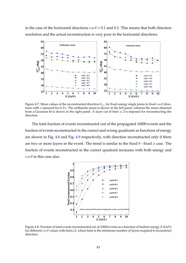
in the case of the horizontal directions cos θ = 0.1 and 0.3. This means that both direction

resolution and the actual reconstruction is very poor in the horizontal directions.

E (GeV)1 2 3 4 5 6 7 8 9 10

(de

g)ar

ithre

cθ

25

30

35

40

45

50

55

60

65

= 0.1θcos = 0.3θcos = 0.5θcos = 0.7θcos = 0.9θcos

Arithmetic mean

E (GeV)1 2 3 4 5 6 7 8 9 10

(de

g)ga

usre

cθ

25

30

35

40

45

50

55

60

65

= 0.1θcos = 0.3θcos

= 0.5θcos

= 0.7θcos = 0.9θcos

Gaussian mean

Figure 4.7: Mean values of the reconstructed direction θrec for fixed energy single pions in fixed cos θ direc-tions with φ smeared fro 0–2π. The arithmetic mean is shown in the left panel, whereas the mean obtainedfrom a Gaussian fit is shown in the right panel. A layer cut of lmin ¥ 2 is imposed for reconstructing thedirection.

The total fraction of events reconstructed out of the propagated 10000 events and the

fraction of events reconstructed in the correct andwrong quadrants as functions of energy

are shown in Fig. 4.8 and Fig. 4.9 respectively, with direction reconstructed only if there

are two or more layers in the event. The trend is similar to the fixed θ - fixed φ case. The

fraction of events reconstructed in the correct quadrant increases with both energy and

cos θ in this case also.

E (GeV)1 2 3 4 5 6 7 8 9 10

Tota

l rec

onst

ruct

ed fr

actio

n

0.3

0.4

0.5

0.6

0.7

0.8

0.9

1

=0.1θcos

=0.3θcos

=0.5θcos

=0.7θcos

=0.9θcos

Total reconstructed fraction of single pion events, raw hit method

Figure 4.8: Fraction of total events reconstructed out of 10000 events as a function of hadron energyE (GeV)for different cos θ values with lmin¥2, where lmin is the minimum number of layers required to reconstructdirection.

83

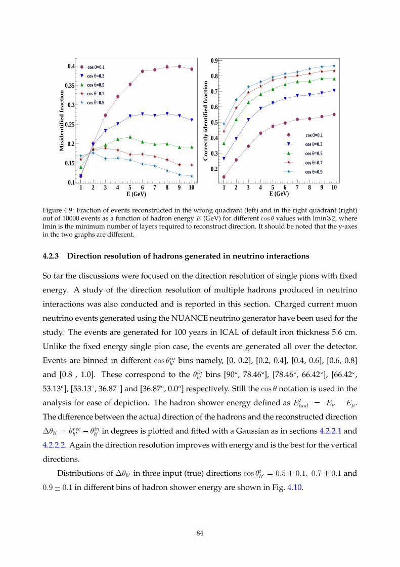
E (GeV)1 2 3 4 5 6 7 8 9 10

Mis

ide

ntifie

d fra

ctio

n

0.1

0.15

0.2

0.25

0.3

0.35

0.4 =0.1θcos

=0.3θcos

=0.5θcos

=0.7θcos

=0.9θcos

E (GeV)1 2 3 4 5 6 7 8 9 10

Co

rre

ctly id

en

tifie

d f

ractio

n

0.2

0.3

0.4

0.5

0.6

0.7

0.8

0.9

=0.1θcos

=0.3θcos

=0.5θcos

=0.7θcos

=0.9θcos

Figure 4.9: Fraction of events reconstructed in the wrong quadrant (left) and in the right quadrant (right)out of 10000 events as a function of hadron energy E (GeV) for different cos θ values with lmin¥2, wherelmin is the minimum number of layers required to reconstruct direction. It should be noted that the y-axesin the two graphs are different.

4.2.3 Direction resolution of hadrons generated in neutrino interactions

So far the discussions were focused on the direction resolution of single pions with fixed

energy. A study of the direction resolution of multiple hadrons produced in neutrino

interactions was also conducted and is reported in this section. Charged current muon

neutrino events generated using the NUANCE neutrino generator have been used for the

study. The events are generated for 100 years in ICAL of default iron thickness 5.6 cm.

Unlike the fixed energy single pion case, the events are generated all over the detector.

Events are binned in different cos θinh1 bins namely, [0, 0.2], [0.2, 0.4], [0.4, 0.6], [0.6, 0.8]

and [0.8 , 1.0]. These correspond to the θinh1 bins [90, 78.46], [78.46, 66.42], [66.42,

53.13], [53.13, 36.87] and [36.87, 0.0] respectively. Still the cos θ notation is used in the

analysis for ease of depiction. The hadron shower energy defined as E 1

had Eν Eµ.

The difference between the actual direction of the hadrons and the reconstructed direction

∆θh1 θrech1 θinh1 in degrees is plotted and fitted with a Gaussian as in sections 4.2.2.1 and

4.2.2.2. Again the direction resolution improves with energy and is the best for the vertical

directions.

Distributions of ∆θh1 in three input (true) directions cos θth1 0.5 0.1, 0.7 0.1 and

0.9 0.1 in different bins of hadron shower energy are shown in Fig. 4.10.

84

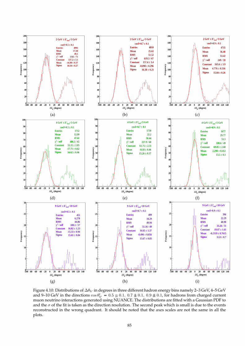
0.1±=0.5 θcosEntries 4993Mean 17.44RMS 49.1

/ ndf 2χ 1361 / 71Constant 3.1± 137.2 Mean 0.37± -16.98 Sigma 0.27± 18.18

(degree)h’θ∆-100 -80 -60 -40 -20 0 20 40 60 80 100 120 140

Fre

qu

en

cy

0

20

40

60

80

100

120

140

160

180

200


/ ndf 2χ 1361 / 71Constant 3.1± 137.2 Mean 0.37± -16.98 Sigma 0.27± 18.18

<3 GeVhad E’≤2 GeV


/ ndf 2χ 619.3 / 67Constant 3.4± 157.4 Mean 0.296± -8.098 Sigma 0.21± 16.38

(degree)h’θ∆-100 -80 -60 -40 -20 0 20 40 60 80 100 120 140

Fre

qu

en

cy

0

20

40

60

80

100

120

140

160

180

200




0.1±=0.9 θcos

Entries 4735

Mean 36.48

RMS 53.42

/ ndf 2χ 249 / 59


Mean 0.316± 4.776 Sigma 0.26± 15.84

(degree)h’θ∆-100 -80 -60 -40 -20 0 20 40 60 80 100 120 140

Fre

qu

en

cy

0

20

40

60

80

100

120

140

160

180

200

0.1±=0.9 θcos

Entries 4735

Mean 36.48

RMS 53.42

/ ndf 2χ 249 / 59


Mean 0.316± 4.776 Sigma 0.26± 15.84


(a) (b) (c)



(degree)h’θ∆-100 -80 -60 -40 -20 0 20 40 60 80 100 120 140

Fre

qu

en

cy

0

10

20

30

40

50

60

70

80

90

100






(degree)h’θ∆-100 -80 -60 -40 -20 0 20 40 60 80 100 120 140

Fre

qu

en

cy

0

10

20

30

40

50

60

70

80

90

100






(degree)h’θ∆-100 -80 -60 -40 -20 0 20 40 60 80 100 120 140

Fre

qu

en

cy

0

10

20

30

40

50

60

70

80

90

100




(d) (e) (f)



(degree)h’θ∆-100 -80 -60 -40 -20 0 20 40 60 80 100 120 140

Fre

qu

en

cy

0

5

10

15

20

25

30






(degree)h’θ∆-100 -80 -60 -40 -20 0 20 40 60 80 100 120 140

Fre

qu

en

cy

0

5

10

15

20

25

30






(degree)h’θ∆-100 -80 -60 -40 -20 0 20 40 60 80 100 120 140

Fre

qu

en

cy

0

5

10

15

20

25

30




(g) (h) (i)

Figure 4.10: Distributions of∆θh1 in degrees in three different hadron energy bins namely 2–3 GeV, 4–5 GeVand 9–10 GeV in the directions cos θth1 0.5 0.1, 0.7 0.1, 0.9 0.1, for hadrons from charged currentmuon neutrino interactions generated using NUANCE. The distributions are fitted with a Gaussian PDF toand the σ of the fit is taken as the direction resolution. The second peak which is small is due to the eventsreconstructed in the wrong quadrant. It should be noted that the axes scales are not the same in all theplots.

85

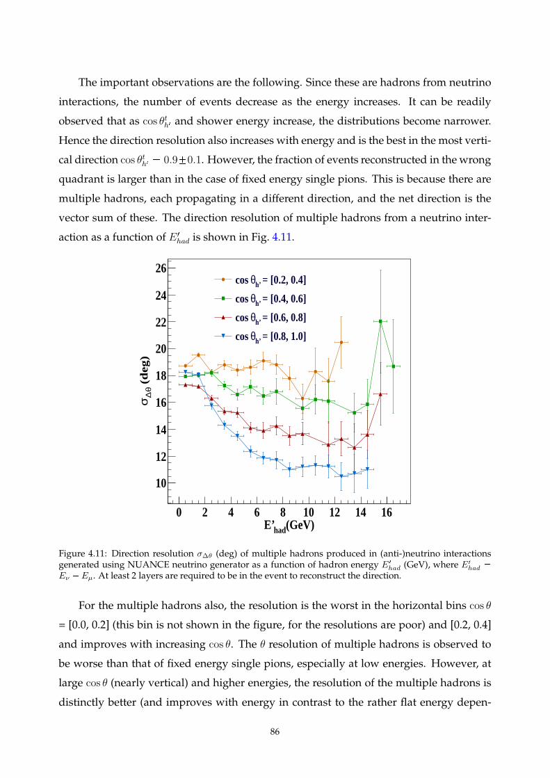
The important observations are the following. Since these are hadrons from neutrino

interactions, the number of events decrease as the energy increases. It can be readily

observed that as cos θth1 and shower energy increase, the distributions become narrower.

Hence the direction resolution also increases with energy and is the best in the most verti-

cal direction cos θth1 0.90.1. However, the fraction of events reconstructed in the wrong

quadrant is larger than in the case of fixed energy single pions. This is because there are

multiple hadrons, each propagating in a different direction, and the net direction is the

vector sum of these. The direction resolution of multiple hadrons from a neutrino inter-

action as a function of E 1

had is shown in Fig. 4.11.

(GeV)hadE’0 2 4 6 8 10 12 14 16

(d

eg

)θ

∆σ

10

12

14

16

18

20

22

24

26 = [0.2, 0.4]h’θcos

= [0.4, 0.6]h’θcos

= [0.6, 0.8]h’θcos

= [0.8, 1.0]h’θcos

Figure 4.11: Direction resolution σ∆θ (deg) of multiple hadrons produced in (anti-)neutrino interactionsgenerated using NUANCE neutrino generator as a function of hadron energy E1

had (GeV), where E1

had

Eν Eµ. At least 2 layers are required to be in the event to reconstruct the direction.

For the multiple hadrons also, the resolution is the worst in the horizontal bins cos θ

= [0.0, 0.2] (this bin is not shown in the figure, for the resolutions are poor) and [0.2, 0.4]

and improves with increasing cos θ. The θ resolution of multiple hadrons is observed to

be worse than that of fixed energy single pions, especially at low energies. However, at

large cos θ (nearly vertical) and higher energies, the resolution of the multiple hadrons is

distinctly better (and improves with energy in contrast to the rather flat energy depen-

86

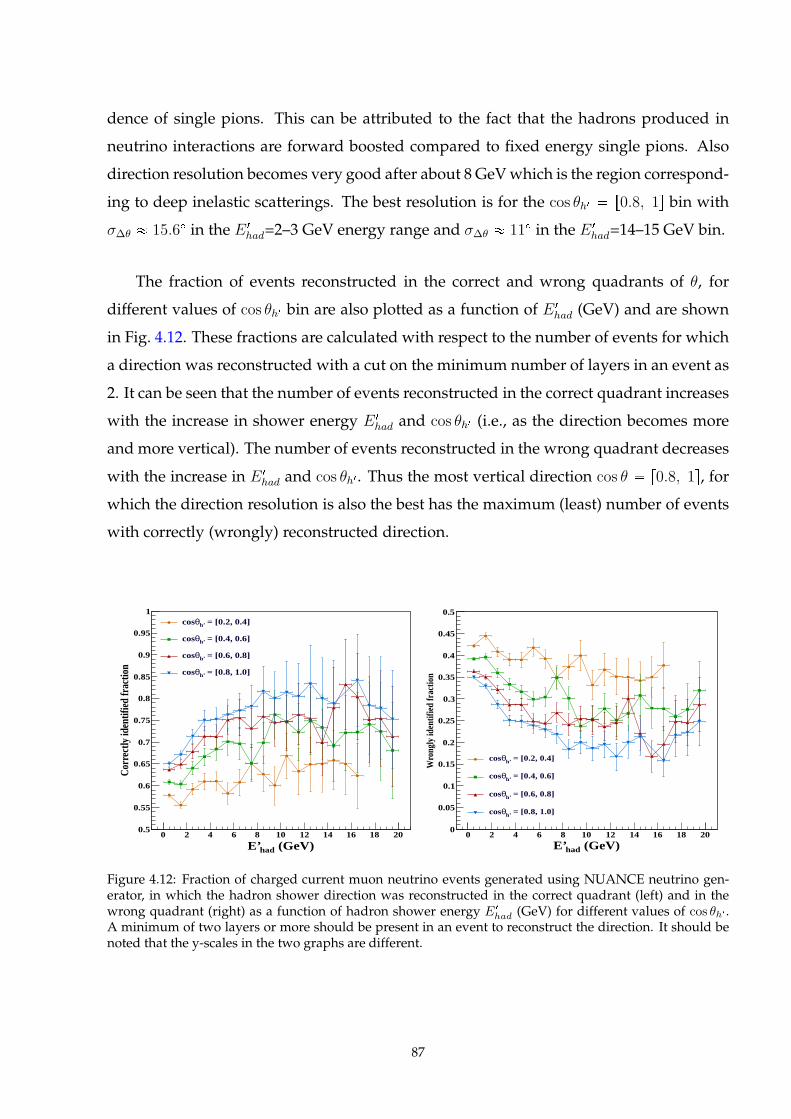
dence of single pions. This can be attributed to the fact that the hadrons produced in

neutrino interactions are forward boosted compared to fixed energy single pions. Also

direction resolution becomes very good after about 8 GeVwhich is the region correspond-

ing to deep inelastic scatterings. The best resolution is for the cos θh1 r0.8, 1s bin with

σ∆θ 15.6 in the E 1

had=2–3 GeV energy range and σ∆θ 11 in the E 1

had=14–15 GeV bin.

The fraction of events reconstructed in the correct and wrong quadrants of θ, for

different values of cos θh1 bin are also plotted as a function of E 1

had (GeV) and are shown

in Fig. 4.12. These fractions are calculated with respect to the number of events for which

a direction was reconstructed with a cut on the minimum number of layers in an event as

2. It can be seen that the number of events reconstructed in the correct quadrant increases

with the increase in shower energy E 1

had and cos θh1 (i.e., as the direction becomes more

and more vertical). The number of events reconstructed in the wrong quadrant decreases

with the increase in E 1

had and cos θh1 . Thus the most vertical direction cos θ r0.8, 1s, for

which the direction resolution is also the best has the maximum (least) number of events

with correctly (wrongly) reconstructed direction.

(GeV)hadE’0 2 4 6 8 10 12 14 16 18 20

Cor

rect

ly id

entif

ied

fract

ion

0.5

0.55

0.6

0.65

0.7

0.75

0.8

0.85

0.9

0.95

1 = [0.2, 0.4]h’θcos

= [0.4, 0.6]h’θcos

= [0.6, 0.8]h’θcos

= [0.8, 1.0]h’θcos

(GeV)hadE’0 2 4 6 8 10 12 14 16 18 20

Wro

ngly

iden

tifie

d fra

ctio

n

0

0.05

0.1

0.15

0.2

0.25

0.3

0.35

0.4

0.45

0.5

= [0.2, 0.4]h’θcos

= [0.4, 0.6]h’θcos

= [0.6, 0.8]h’θcos

= [0.8, 1.0]h’θcos

Figure 4.12: Fraction of charged current muon neutrino events generated using NUANCE neutrino gen-erator, in which the hadron shower direction was reconstructed in the correct quadrant (left) and in thewrong quadrant (right) as a function of hadron shower energy E1

had (GeV) for different values of cos θh1 .A minimum of two layers or more should be present in an event to reconstruct the direction. It should benoted that the y-scales in the two graphs are different.

87

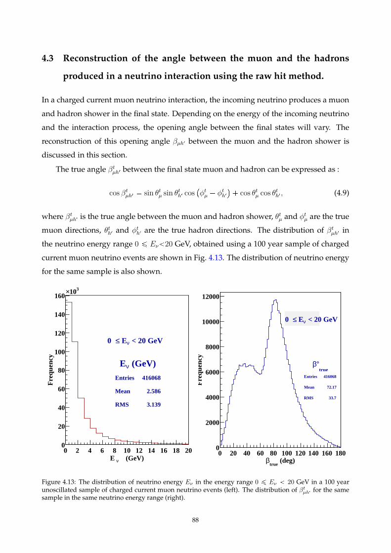
4.3 Reconstruction of the angle between the muon and the hadrons

produced in a neutrino interaction using the raw hit method.

In a charged current muon neutrino interaction, the incoming neutrino produces a muon

and hadron shower in the final state. Depending on the energy of the incoming neutrino

and the interaction process, the opening angle between the final states will vary. The

reconstruction of this opening angle βµh1 between the muon and the hadron shower is

discussed in this section.

The true angle βtµh1 between the final state muon and hadron can be expressed as :

cos βtµh1 sin θtµ sin θth1 cos

φtµ φth1

cos θtµ cos θth1, (4.9)

where βtµh1 is the true angle between the muon and hadron shower, θtµ and φtµ are the true

muon directions, θth1 and φth1 are the true hadron directions. The distribution of βtµh1 in

the neutrino energy range 0 ¤ Eν 20 GeV, obtained using a 100 year sample of charged

current muon neutrino events are shown in Fig. 4.13. The distribution of neutrino energy

for the same sample is also shown.

(GeV)νE

Entries 416068

Mean 2.586

RMS 3.139

(GeV)νE0 2 4 6 8 10 12 14 16 18 20

Fre

quen

cy

0

20

40

60

80

100

120

140

160310×

(GeV)νE

Entries 416068

Mean 2.586

RMS 3.139

< 20 GeVν E≤0

true°β

Entries 416068

Mean 72.17

RMS 33.7

(deg)true

β0 20 40 60 80 100 120 140 160 180

Fre

quen

cy

0

2000

4000

6000

8000

10000

12000

true°β

Entries 416068

Mean 72.17

RMS 33.7

< 20 GeV ν E≤0

Figure 4.13: The distribution of neutrino energy Eν in the energy range 0 ¤ Eν 20 GeV in a 100 yearunoscillated sample of charged current muon neutrino events (left). The distribution of βt

µh1 for the samesample in the same neutrino energy range (right).

88

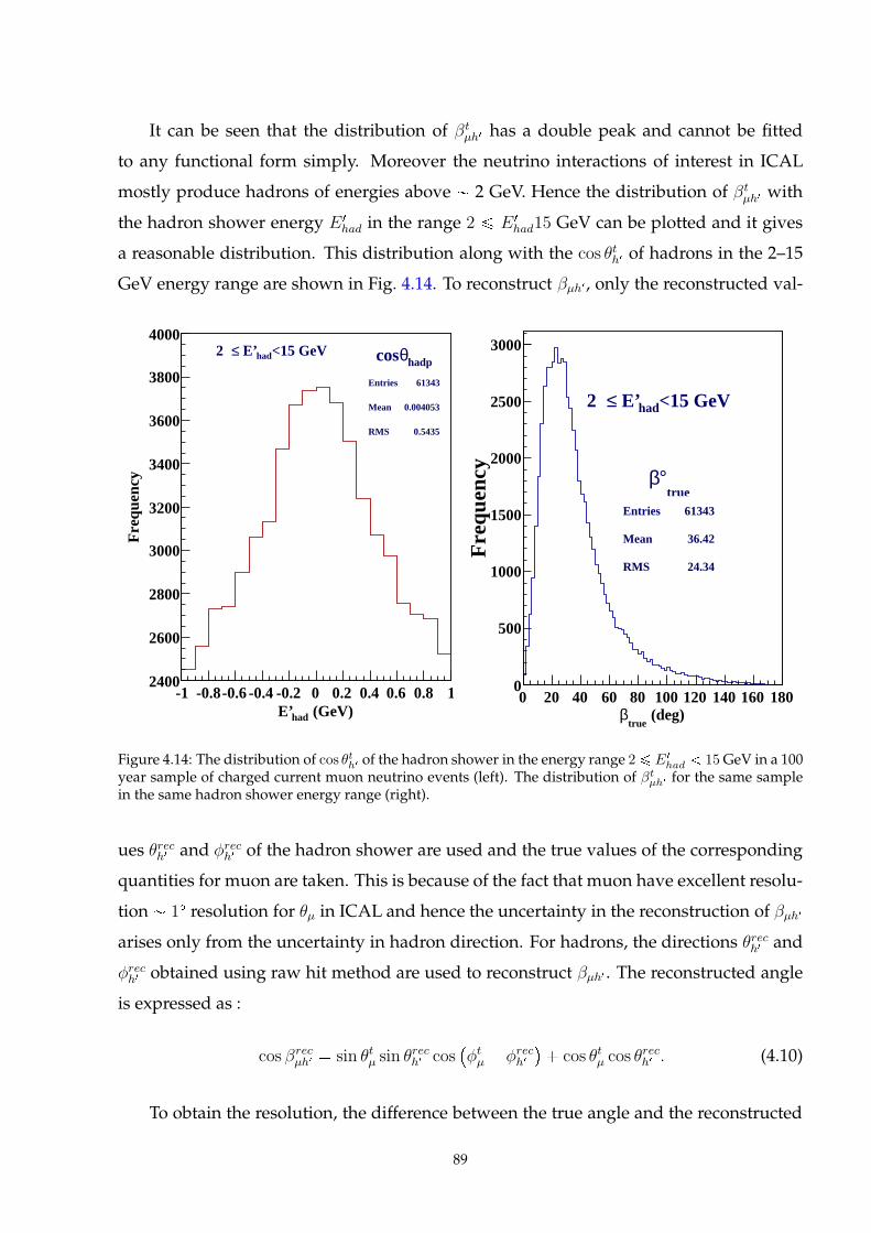
It can be seen that the distribution of βtµh1 has a double peak and cannot be fitted

to any functional form simply. Moreover the neutrino interactions of interest in ICAL

mostly produce hadrons of energies above 2 GeV. Hence the distribution of βtµh1 with

the hadron shower energy E 1

had in the range 2 ¤ E 1

had15 GeV can be plotted and it gives

a reasonable distribution. This distribution along with the cos θth1 of hadrons in the 2–15

GeV energy range are shown in Fig. 4.14. To reconstruct βµh1 , only the reconstructed val-

hadpθcos

Entries 61343

Mean 0.004053

RMS 0.5435

(GeV)hadE’-1 -0.8-0.6 -0.4 -0.2 0 0.2 0.4 0.6 0.8 1

Fre

quen

cy

2400

2600

2800

3000

3200

3400

3600

3800

4000

hadpθcos

Entries 61343

Mean 0.004053

RMS 0.5435

<15 GeVhad E’≤2

true°β

Entries 61343

Mean 36.42

RMS 24.34

(deg)true

β0 20 40 60 80 100 120 140 160 180

Fre

quen

cy

0

500

1000

1500

2000

2500

3000

true°β

Entries 61343

Mean 36.42

RMS 24.34

<15 GeVhad E’≤2

Figure 4.14: The distribution of cos θth1 of the hadron shower in the energy range 2 ¤ E1

had 15GeV in a 100year sample of charged current muon neutrino events (left). The distribution of βt

µh1 for the same samplein the same hadron shower energy range (right).

ues θrech1 and φrech1 of the hadron shower are used and the true values of the corresponding

quantities for muon are taken. This is because of the fact that muon have excellent resolu-

tion 1 resolution for θµ in ICAL and hence the uncertainty in the reconstruction of βµh1

arises only from the uncertainty in hadron direction. For hadrons, the directions θrech1 and

φrech1 obtained using raw hit method are used to reconstruct βµh1 . The reconstructed angle

is expressed as :

cos βrecµh1 sin θtµ sin θrech1 cos

φtµ φrech1

cos θtµ cos θrech1 . (4.10)

To obtain the resolution, the difference between the true angle and the reconstructed

89

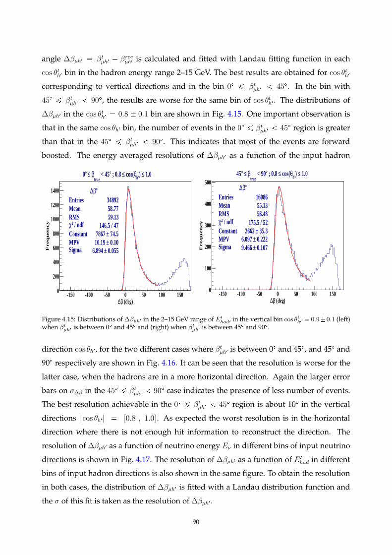
angle ∆βµh1 βtµh1 βrecµh1 is calculated and fitted with Landau fitting function in each

cos θth1 bin in the hadron energy range 2–15 GeV. The best results are obtained for cos θth1

corresponding to vertical directions and in the bin 0 ¤ βtµh1 45. In the bin with

45 ¤ βtµh1 90, the results are worse for the same bin of cos θth1 . The distributions of

∆βµh1 in the cos θth1 0.8 0.1 bin are shown in Fig. 4.15. One important observation is

that in the same cos θh1 bin, the number of events in the 0 ¤ βtµh1 45 region is greater

than that in the 45 ¤ βtµh1 90. This indicates that most of the events are forward

boosted. The energy averaged resolutions of ∆βµh1 as a function of the input hadron

°β∆Entries 34892Mean 58.77RMS 59.13

/ ndf 2χ 146.5 / 47Constant 74.5± 7867 MPV 0.10± 10.19 Sigma 0.055± 6.894

(deg)β∆-150 -100 -50 0 50 100 150

Fre

qu

en

cy

0

200

400

600

800

1000

1200

1400 °β∆Entries 34892Mean 58.77RMS 59.13


1.0≤) h’θ cos(≤ ; 0.8 ° < 45true

β ≤ °0

°β∆Entries 16086Mean 55.13RMS 56.48


(deg)β∆-150 -100 -50 0 50 100 150

Fre

qu

en

cy

0

100

200

300

400

500°β∆



1.0≤) h’θ cos(≤ ; 0.8 ° < 90true

β ≤ °45

Figure 4.15: Distributions of∆βµh1 in the 2–15 GeV range of E1

had, in the vertical bin cos θth1 0.90.1 (left)when βt

µh1 is between 0 and 45 and (right) when βtµh1 is between 45 and 90.

direction cos θh1 , for the two different cases where βtµh1 is between 0 and 45, and 45 and

90 respectively are shown in Fig. 4.16. It can be seen that the resolution is worse for the

latter case, when the hadrons are in a more horizontal direction. Again the larger error

bars on σ∆β in the 45 ¤ βtµh1 90 case indicates the presence of less number of events.

The best resolution achievable in the 0 ¤ βtµh1 45 region is about 10 in the vertical

directions | cos θh1| r0.8 , 1.0s. As expected the worst resolution is in the horizontal

direction where there is not enough hit information to reconstruct the direction. The

resolution of ∆βµh1 as a function of neutrino energy Eν in different bins of input neutrino

directions is shown in Fig. 4.17. The resolution of ∆βµh1 as a function of E 1

had in different

bins of input hadron directions is also shown in the same figure. To obtain the resolution

in both cases, the distribution of ∆βµh1 is fitted with a Landau distribution function and

the σ of this fit is taken as the resolution of ∆βµh1 .

90

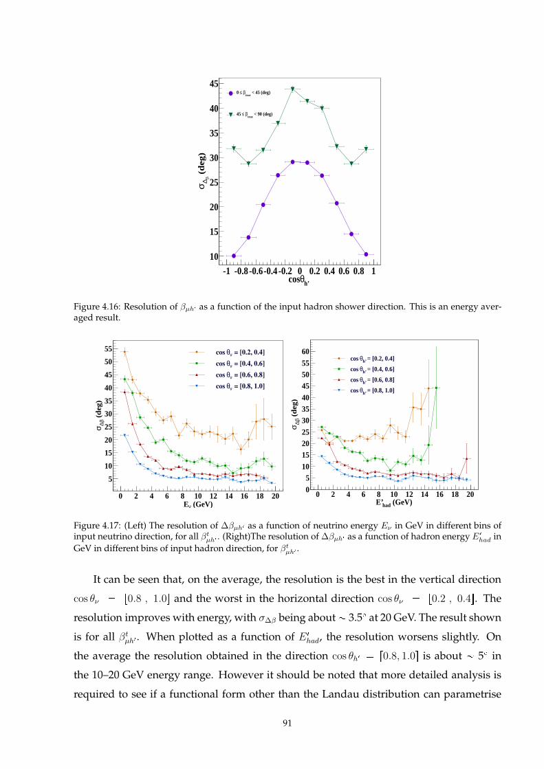
h’θcos-1 -0.8-0.6-0.4-0.2 0 0.2 0.4 0.6 0.8 1

(d

eg

)β

∆σ

10

15

20

25

30

35

40

45 < 45 (deg)

trueβ ≤0

< 90 (deg)true

β ≤45

Figure 4.16: Resolution of βµh1 as a function of the input hadron shower direction. This is an energy aver-aged result.

(GeV)νE0 2 4 6 8 10 12 14 16 18 20

(d

eg

)β∆

σ

5

10

15

20

25

30

35

40

45

50

55 = [0.2, 0.4]νθcos

= [0.4, 0.6]νθcos

= [0.6, 0.8]νθcos

= [0.8, 1.0]νθcos

(GeV)hadE’0 2 4 6 8 10 12 14 16 18 20

(d

eg

)β∆

σ

0

510

152025

303540

455055

60 = [0.2, 0.4]h’θcos

= [0.4, 0.6]h’θcos

= [0.6, 0.8]h’θcos

= [0.8, 1.0]h’θcos

Figure 4.17: (Left) The resolution of ∆βµh1 as a function of neutrino energy Eν in GeV in different bins ofinput neutrino direction, for all βt

µh1 . (Right)The resolution of∆βµh1 as a function of hadron energy E1

had in

GeV in different bins of input hadron direction, for βtµh1 .

It can be seen that, on the average, the resolution is the best in the vertical direction

cos θν r0.8 , 1.0s and the worst in the horizontal direction cos θν r0.2 , 0.4s. The

resolution improves with energy, with σ∆β being about 3.5 at 20 GeV. The result shown

is for all βtµh1 . When plotted as a function of E 1

had, the resolution worsens slightly. On

the average the resolution obtained in the direction cos θh1 r0.8, 1.0s is about 5 in

the 10–20 GeV energy range. However it should be noted that more detailed analysis is

required to see if a functional form other than the Landau distribution can parametrise

91

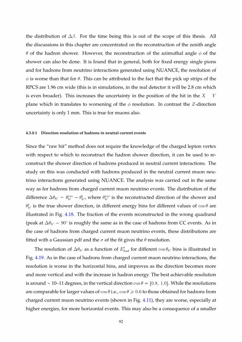
the distribution of ∆β. For the time being this is out of the scope of this thesis. All

the discussions in this chapter are concentrated on the reconstruction of the zenith angle

θ of the hadron shower. However, the reconstruction of the azimuthal angle φ of the

shower can also be done. It is found that in general, both for fixed energy single pions

and for hadrons from neutrino interactions generated using NUANCE, the resolution of

φ is worse than that for θ. This can be attributed to the fact that the pick up strips of the

RPCS are 1.96 cm wide (this is in simulations, in the real detector it will be 2.8 cm which

is even broader). This increases the uncertainty in the position of the hit in the X Y

plane which in translates to worsening of the φ resolution. In contrast the Z-direction

uncertainty is only 1 mm. This is true for muons also.

4.3.0.1 Direction resolution of hadrons in neutral current events

Since the “raw hit” method does not require the knowledge of the charged lepton vertex

with respect to which to reconstruct the hadron shower direction, it can be used to re-

construct the shower direction of hadrons produced in neutral current interactions. The

study on this was conducted with hadrons produced in the neutral current muon neu-

trino interactions generated using NUANCE. The analysis was carried out in the same

way as for hadrons from charged current muon neutrino events. The distribution of the

difference ∆θh1 θrech1 θth1 , where θrech1 is the reconstructed direction of the shower and

θth1 is the true shower direction, in different energy bins for different values of cos θ are

illustrated in Fig. 4.18. The fraction of the events reconstructed in the wrong quadrand

(peak at ∆θh1 90 is roughly the same as in the case of hadrons from CC events. As in

the case of hadrons from charged current muon neutrino events, these distributions are

fitted with a Gaussian pdf and the σ of the fit gives the θ resolution.

The resolution of ∆θh1 as a function of E 1

had for different cos θh1 bins is illustrated in

Fig. 4.19. As in the case of hadrons from charged current muon neutrino interactions, the

resolution is worse in the horizontal bins, and improves as the direction becomes more

and more vertical and with the increase in hadron energy. The best achievable resolution

is around 10–11 degrees, in the vertical direction cos θ r0.8, 1.0s. While the resolutions

are comparable for larger values of cos θ i.e., cos θ ¥ 0.6 to those obtained for hadrons from

charged current muon neutrino events (shown in Fig. 4.11), they are worse, especially at

higher energies, for more horizontal events. This may also be a consequence of a smaller

92

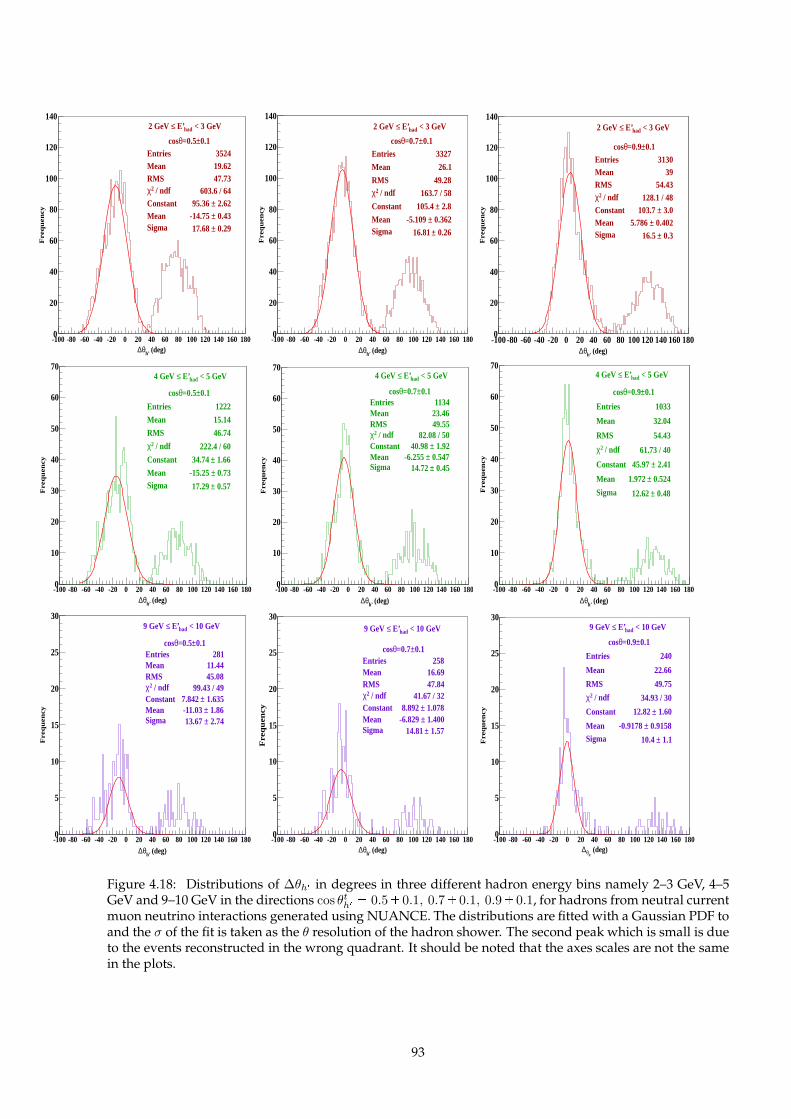
0.1±=0.5θcosEntries 3524Mean 19.62RMS 47.73


(deg)h’θ∆-100 -80 -60 -40 -20 0 20 40 60 80 100 120 140 160 180

Fre

qu

en

cy

0

20

40

60

80

100

120

140



< 3 GeVhad E’≤2 GeV

0.1±=0.7θcosEntries 3327

Mean 26.1

RMS 49.28 / ndf 2χ 163.7 / 58


Mean 0.362± -5.109 Sigma 0.26± 16.81

(deg)h’θ∆-100 -80 -60 -40 -20 0 20 40 60 80 100 120 140 160 180

Fre

qu

en

cy

0

20

40

60

80

100

120

140

0.1±=0.7θcosEntries 3327

Mean 26.1

RMS 49.28 / ndf 2χ 163.7 / 58


Mean 0.362± -5.109 Sigma 0.26± 16.81


0.1±=0.9θcosEntries 3130Mean 39RMS 54.43


(deg)h’θ∆-100 -80 -60 -40 -20 0 20 40 60 80 100 120 140 160 180

Fre

qu

en

cy

0

20

40

60

80

100

120

140

0.1±=0.9θcosEntries 3130Mean 39RMS 54.43



0.1±=0.5θcos

Entries 1222

Mean 15.14

RMS 46.74

/ ndf 2χ 222.4 / 60


Mean 0.73± -15.25 Sigma 0.57± 17.29

(deg)h’θ∆-100 -80 -60 -40 -20 0 20 40 60 80 100 120 140 160 180

Fre

qu

en

cy

0

10

20

30

40

50

60

70

0.1±=0.5θcos

Entries 1222

Mean 15.14

RMS 46.74

/ ndf 2χ 222.4 / 60


Mean 0.73± -15.25 Sigma 0.57± 17.29




(deg)h’θ∆-100 -80 -60 -40 -20 0 20 40 60 80 100 120 140 160 180

Fre

qu

en

cy

0

10

20

30

40

50

60

70




0.1±=0.9θcos

Entries 1033

Mean 32.04

RMS 54.43

/ ndf 2χ 61.73 / 40


Mean 0.524± 1.972

Sigma 0.48± 12.62

(deg)h’θ∆-100 -80 -60 -40 -20 0 20 40 60 80 100 120 140 160 180

Fre

qu

en

cy

0

10

20

30

40

50

60

70

0.1±=0.9θcos

Entries 1033

Mean 32.04

RMS 54.43

/ ndf 2χ 61.73 / 40


Mean 0.524± 1.972

Sigma 0.48± 12.62




(deg)h’θ∆-100 -80 -60 -40 -20 0 20 40 60 80 100 120 140 160 180

Fre

qu

en

cy

0

5

10

15

20

25

30






(deg)h’θ∆-100 -80 -60 -40 -20 0 20 40 60 80 100 120 140 160 180

Fre

qu

en

cy

0

5

10

15

20

25

30




0.1±=0.9θcos

Entries 240

Mean 22.66

RMS 49.75

/ ndf 2χ 34.93 / 30


Mean 0.9158± -0.9178 Sigma 1.1± 10.4

(deg)h’θ∆

-100 -80 -60 -40 -20 0 20 40 60 80 100 120 140 160 180

Fre

qu

en

cy

0

5

10

15

20

25

30

0.1±=0.9θcos

Entries 240

Mean 22.66

RMS 49.75

/ ndf 2χ 34.93 / 30


Mean 0.9158± -0.9178 Sigma 1.1± 10.4


Figure 4.18: Distributions of ∆θh1 in degrees in three different hadron energy bins namely 2–3 GeV, 4–5GeV and 9–10 GeV in the directions cos θth1 0.50.1, 0.70.1, 0.90.1, for hadrons from neutral currentmuon neutrino interactions generated using NUANCE. The distributions are fitted with a Gaussian PDF toand the σ of the fit is taken as the θ resolution of the hadron shower. The second peak which is small is dueto the events reconstructed in the wrong quadrant. It should be noted that the axes scales are not the samein the plots.

93

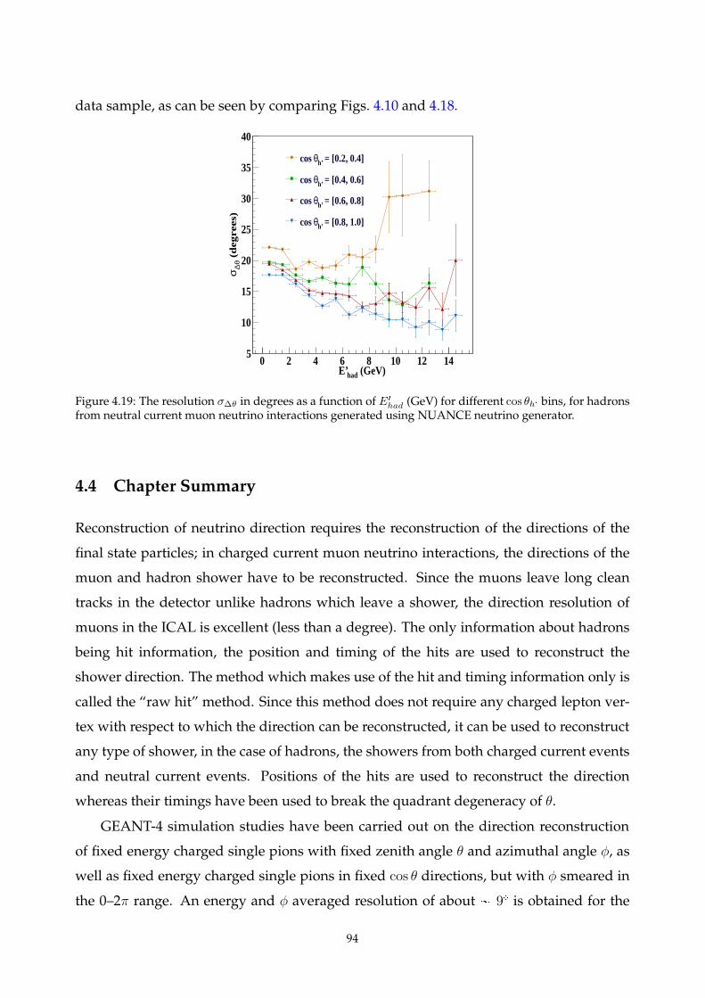
data sample, as can be seen by comparing Figs. 4.10 and 4.18.

(GeV)hadE’0 2 4 6 8 10 12 14

(d

eg

ree

s)

θ∆

σ

5

10

15

20

25

30

35

40

= [0.2, 0.4]h’θcos

= [0.4, 0.6]h’θcos

= [0.6, 0.8]h’θcos

= [0.8, 1.0]h’θcos

Figure 4.19: The resolution σ∆θ in degrees as a function of E1

had (GeV) for different cos θh1 bins, for hadronsfrom neutral current muon neutrino interactions generated using NUANCE neutrino generator.

4.4 Chapter Summary

Reconstruction of neutrino direction requires the reconstruction of the directions of the

final state particles; in charged current muon neutrino interactions, the directions of the

muon and hadron shower have to be reconstructed. Since the muons leave long clean

tracks in the detector unlike hadrons which leave a shower, the direction resolution of

muons in the ICAL is excellent (less than a degree). The only information about hadrons

being hit information, the position and timing of the hits are used to reconstruct the

shower direction. The method which makes use of the hit and timing information only is

called the “raw hit” method. Since this method does not require any charged lepton ver-

tex with respect to which the direction can be reconstructed, it can be used to reconstruct

any type of shower, in the case of hadrons, the showers from both charged current events

and neutral current events. Positions of the hits are used to reconstruct the direction

whereas their timings have been used to break the quadrant degeneracy of θ.

GEANT-4 simulation studies have been carried out on the direction reconstruction

of fixed energy charged single pions with fixed zenith angle θ and azimuthal angle φ, as

well as fixed energy charged single pions in fixed cos θ directions, but with φ smeared in

the 0–2π range. An energy and φ averaged resolution of about 9 is obtained for the

94

θ 30 case and 9.8 in the θ 150 case, in the 1–10 GeV energy range. In the case

where different cos θ directions are considered the best θ resolution is obtained for the

cos θ value 0.9. At 1 GeV the resolution is about 9.38 0.17 and 8.68 0.11 at 10 GeV,

at this cos θ.

Simulation studies of direction reconstruction of hadron showers from neutrino events

generated using NUANCE neutrino generator were also done. Both charged current

muon neutrino and neutral current muon neutrino events have been used for this study.

The resolutions are again found to be the best in the vertical direction cos θ r0.8, 1s

with σ∆θ 15.6 in the E 1

had 2.5 0.5 GeV bin and 11 in the E 1

had 14.5 0.5 GeV

bin. It decreases as cos θh1 decreases and is worse for the hadrons in the most horizontal

direction, i.e., in the cos θh1 r0, 0.2s bin. It should be noted that these resolutions corre-

spond to the actual polar angle, and not the angle with respect to the neutrino or charged

lepton. The resolution is therefore worse (both for hadrons and muons) in the horizontal

direction, due to the geometry of ICAL, with its horizontal layers and X Y magnetic

field. Hence the events in which either the muon or the final state hadrons (or both) are

mostly in the horizontal direction will be poorly reconstructed.

For hadrons from neutral current muon neutrino events also the trend of θ resolution

is the same, with the resolution being the best in the cos θh1 r0.8, 1s direction. A resolu-

tion of 16.5 is obtained in the 2–3 GeV E 1

had bin and 10 is obtained in the 12–15 GeV

energy range.

The resolution of the opening angle βµh1 between the muon and the hadrons in the

final state of a charged current muon neutrino interaction is also obtained using the raw

hit method. For this purpose the reconstructed values of only the hadron θ and φ are used;

the true values of the muon direction are taken for the analysis. The resolution σ∆β is the

best in the | cos θh1| r0.8, 1s bin, 10; the 0 ¤ βtrue 45 region is better compared to

the 45 ¤ βtrue 90 region. The energy dependence of the resolution of βµh1 is such that

a fit to the ∆βµh1 histogram with a Landau distribution in the Eν 2.5 0.5 GeV region

yields a resolution of 10 and 3.3 in the Eν 2.5 0.5 in the cos θν r0.8, 1s bin.

Thus it can be seen that the simulation studies can give a good insight into the di-

rection reconstruction of hadrons which in turn will help in the reconstruction of the

direction of the incoming neutrino. It can be seen that the uncertainty in the reconstruc-

tion of the neutrino direction is driven by that in the reconstruction of hadron direction.

Hence, any change in geometry, like varying the strip width or any new algorithm to

95

improve the shower reconstruction and the direction resolution has to be probed. Even

then the results of this study give a good idea of what the hadron direction will be like

in the ICAL detector. Currently only the muon energy, direction and the hadron energy

are being used as the observables to bin the events in the oscillation physics studies using

the ICAL. The effect of adding hadron direction as a fourth observable is worth studying

since the addition of hadron energy has proved to significantly improve the sensitivity of

the ICAL to oscillation parameters. Also the binning of events in the LE of the neutrino

is always of interest and for this, the reconstruction of both hadron energy and direction

are necessary inputs in order to reconstruct fully the L and E of the neutrino from the

corresponding charged current lepton and hadron informations.

96

5Brief review of muon response in

ICAL

5.1 Overview

The main interaction processes of interest in the ICAL detector being the charged current

interactions of muon neutrinos and anti-neutrinos (i.e., CC interactions of νµ and νµ), it

is necessary to reconstruct the momentum and direction of the final state muon to recon-

struct the incoming neutrino parameters. Also the charge of the muon has to be deter-

mined by the direction of its curvature in the magnetic field, since this is the crucial infor-

mation which determines whether the interaction was that of a neutrino or anti-neutrino

and hence forms the basic technique for mass hierarchy distinction. GEANT4 based sim-

ulation studies to characterise the muon responses and reconstruction and charge identi-

fication efficiencies of the ICAL detector have been performed and have been reported in

Refs. [22, 108]. The responses and efficiencies of muons in the central region of the ICAL

detector have been tabulated into a look up table and are used in the ICAL oscillation

sensitivity analyses. These values as can be seen in the following sections are the best

values of muon responses and yield the best oscillation sensitivities because of the uni-

form magnetic field of 1.5 T. The main highlights of the muon responses in the central of

the ICAL detector discussed in [22] are presented in this Chapter for completeness, since

they are used in the analysis presented in Chapter 6. In addition, a brief discussion on

separating charged current muon neutrino (ccmu) events from charged current electron

and neutral current events (cce and nc) is also presented in this Chapter.

5.2 Muons and tracks

The most important quality of muons propagating in ICAL is that they leave clean tracks

in the detector unlike the showers by hadrons. This is because of these particles being

minimum ionising at the energies of interest to ICAL. As mentioned in Chapter 3, a

charged particle leaves a “hit” in the detector, which carries both position and timing

informations; the px, yq co-ordinates obtained from the pick up strips, z from the layer,

and timing with respect to a trigger. Muons in ICAL leave one hit per layer on the av-

erage hence avoiding the ghost hit problem seen with hadrons; in addition, they leave a

long track in the detector. The reconstruction of muons in the ICAL are done in different

steps which include finding the tracks from hits and fitting the tracks.

5.2.1 Track finding

The possible pairing of all adjacent x and y hits in a layer give clusters.; a tracklet com-

prises clusters in a few successive layers. Using a simple curve fitting algorithm, tracklets

are found by searching for clusters in three adjacent layers. Nearby tracklets are joined

together to form a track and the longest possible track in an event is obtained by the it-

eration of this process [132]. The direction of the track is determined by averaging the x

and y timings in a plane. To reduce the misidentification of a hadron shower or noise as

a muon track the event is required to satisfy the criterion that it should contain at least 5

layers in the muon-like track. For such events, the clusters in each plane are averaged to

a single hit per plane and the position and timing information of this average hit point

are passed to the track fitter.

5.2.2 Track fitting

Track fitting in ICAL is done using a Kalman filter [133] based algorithm to take into

account the bending of tracks in the presence of magnetic field and the effects due to

energy losses during propagation. Since the tracks are bent a simple linear fit cannot

be applied to fit the tracks and obtain the direction of the muon from it. The Kalman

filter algorithm [133–135] treats a track as a state vector paramatrised by hit position,

track direction and the particle momentum at a particular position. The starting state

vector is defined as X0 px, y, dxdz, dydz, qpq, where px, y, zq is the position of the

first hit recorded by the finder. The charge weighted inverse momentum qp is taken to

be zero at this stage. The initial track direction is calculated using the first two layers

of the event assuming that it is straight in this section. This initial state vector X0 is

then extrapolated into the next layer using a 5 5 propagator matrix F , whose elements

contain information about themagnetic field according to the magnetic fieldmap of ICAL

98

discussed in Chapter 2 and energy loss of the particle in iron according to Bethe-Bloch

equation [120].

The estimated value of the state vector after k planes is given by Xk Fk1Xk1

uk1. Here u represents the process noise which gives information about multiple scat-

tering and energy loss by the muon. The propagator matrix is calculated for every pair

of detector planes. The state covariance matrix C contains the expected error in the state

vector. Iterative comparisons of the actual hit location and the extrapolated point are

done till they are close enough to call the fit to the track a good one. Further extrapola-

tion of the track backwards is done to half the thickness of the iron layer to determine

the interaction vertex (assumed to be at the centre of the iron plate). The best fit value

of the muon momentum at the vertex is obtained as the reconstructed momentum (both

magnitude and direction). The quantity qp determines the magnitude of the momentum

at the vertex and gives the charge of the muon, whereas dxdz and dydz give cos θ and φ

of the muon. To obtain best reconstructed values a loose cut of χ2ndf 10 is imposed; a

tighter constraint does not alter the results significantly.

5.3 Muon resolutions and efficiencies

As in the case of hadrons, GEANT4 based simulation studies have been conducted to es-

timate the muon resolutions and efficiencies in the ICAL detector, especially in the central

region of eachmodule. Fixed energy single muons propagating from vertices randomised

over a region of -4 m ¤ x ¤ 4 m, -4 m ¤ y ¤ 4 m and -4 m ¤ z ¤ 4 m with the origin in

the center of the central module are used for this analysis. The muons being minimum

ionising particles will travel long distances in the detector that some of the tracks may

even go out of the detector volume depending on the energy (mostly around pin ¥ 6

GeV/c), direction and the vertex of the muons. Both fully and partially contained events

are analysed together here.

Both µ and µ are propagated in the detector at fixed momenta pin in fixed cos θ

bins with φ smeared from 0–2π. The reconstructed muon momentum distribution for

ppin, cos θq p5 GeV/c, 0.65q is shown in Fig. 5.1. Since the distributions are similar for

both µ and µ, only µ have been used further to determine momentum and direction

resolutions. The results of this analysis was tabulated as a look-up table and this table is

used in the physics simulation studies discussed in Chapter 6. The detailed analysis of

99

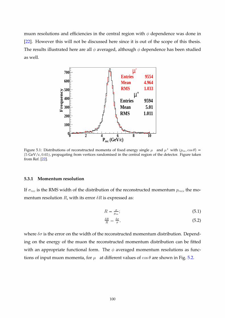
muon resolutions and efficiencies in the central region with φ dependence was done in

[22]. However this will not be discussed here since it is out of the scope of this thesis.

The results illustrated here are all φ averaged, although φ dependence has been studied

as well.


(GeV/c)recP0 2 4 6 8 10

Fre

qu

en

cy

0

100

200

300

400

500

600

700Entries 9554Mean 4.964RMS 1.033

-µ



+µ

Figure 5.1: Distributions of reconstructed momenta of fixed energy single µ and µ with ppin, cos θq p5 GeV/c, 0.65q, propagating from vertices randomised in the central region of the detector. Figure takenfrom Ref. [22].

5.3.1 Momentum resolution

If σrec is the RMS width of the distribution of the reconstructed momentum prec, the mo-

mentum resolution R, with its error δR is expressed as:

R

σpin

; (5.1)

δRR

δσσ, (5.2)

where δσ is the error on the width of the reconstructed momentum distribution. Depend-

ing on the energy of the muon the reconstructed momentum distribution can be fitted

with an appropriate functional form. The φ averaged momentum resolutions as func-

tions of input muon momenta, for µ at different values of cos θ are shown in Fig. 5.2.

100

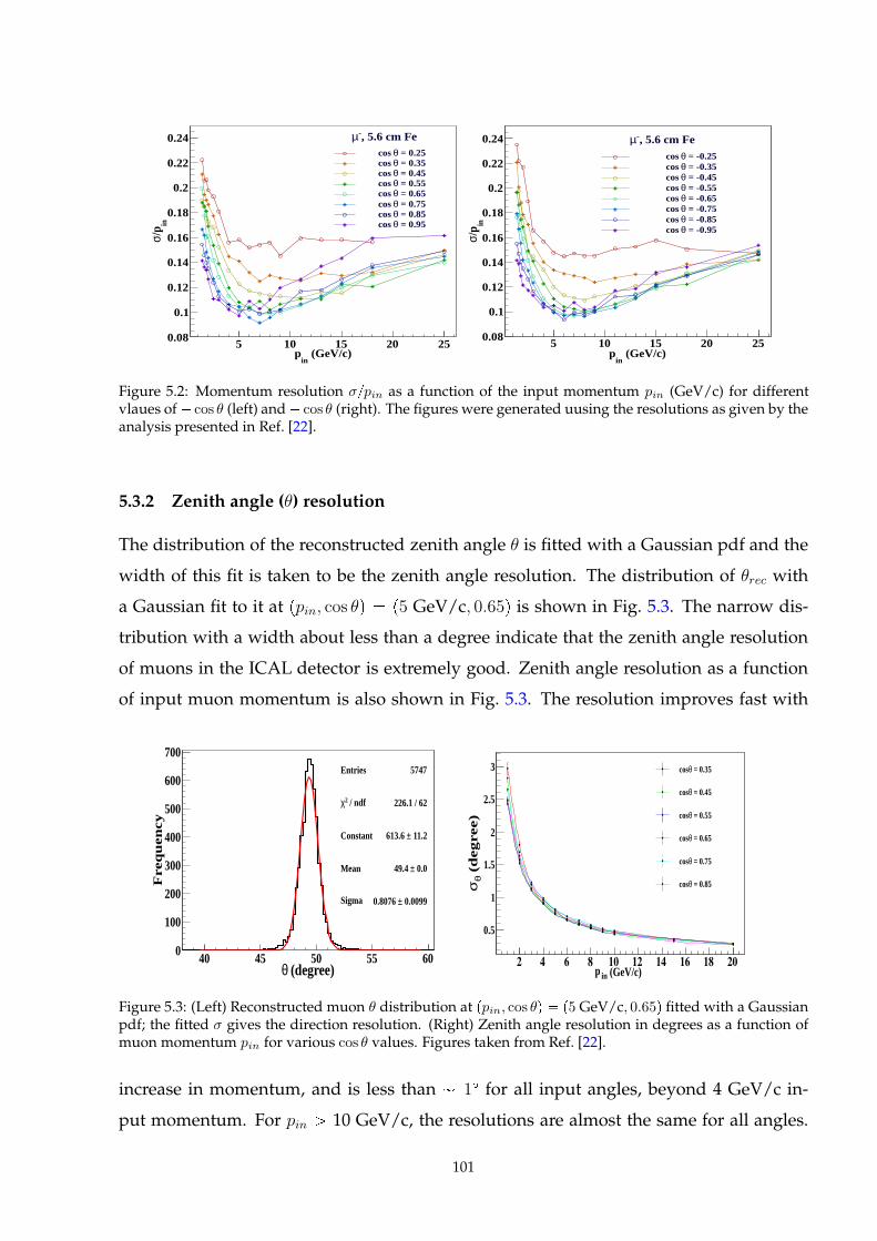
(GeV/c)in

p5 10 15 20 25

in/pσ

0.08

0.1

0.12

0.14

0.16

0.18

0.2

0.22

0.24 = 0.25θcos = 0.35θcos = 0.45θcos = 0.55θcos = 0.65θcos = 0.75θcos = 0.85θcos = 0.95θcos

, 5.6 cm Fe-µ

(GeV/c)in

p5 10 15 20 25

in/pσ

0.08

0.1

0.12

0.14

0.16

0.18

0.2

0.22

0.24

= -0.25θcos = -0.35θcos = -0.45θcos = -0.55θcos = -0.65θcos = -0.75θcos = -0.85θcos = -0.95θcos

, 5.6 cm Fe-µ

Figure 5.2: Momentum resolution σpin as a function of the input momentum pin (GeV/c) for differentvlaues of cos θ (left) and cos θ (right). The figures were generated uusing the resolutions as given by theanalysis presented in Ref. [22].

5.3.2 Zenith angle (θ) resolution

The distribution of the reconstructed zenith angle θ is fitted with a Gaussian pdf and the

width of this fit is taken to be the zenith angle resolution. The distribution of θrec with

a Gaussian fit to it at ppin, cos θq p5 GeV/c, 0.65q is shown in Fig. 5.3. The narrow dis-

tribution with a width about less than a degree indicate that the zenith angle resolution

of muons in the ICAL detector is extremely good. Zenith angle resolution as a function

of input muon momentum is also shown in Fig. 5.3. The resolution improves fast with

Entries 5747

/ ndf 2χ 226.1 / 62


Mean 0.0± 49.4

Sigma 0.0099± 0.8076

(degree)θ40 45 50 55 60

Fre

que

ncy

0

100

200

300

400

500

600

700Entries 5747

/ ndf 2χ 226.1 / 62


Mean 0.0± 49.4

Sigma 0.0099± 0.8076

(GeV/c)inp2 4 6 8 10 12 14 16 18 20

(de

gre

e)

θσ

0.5

1

1.5

2

2.5

3 = 0.35θ cos

= 0.45θ cos

= 0.55θ cos

= 0.65θ cos

= 0.75θ cos

= 0.85θ cos

Figure 5.3: (Left) Reconstructed muon θ distribution at ppin, cos θq p5 GeV/c, 0.65q fitted with a Gaussianpdf; the fitted σ gives the direction resolution. (Right) Zenith angle resolution in degrees as a function ofmuon momentum pin for various cos θ values. Figures taken from Ref. [22].

increase in momentum, and is less than 1 for all input angles, beyond 4 GeV/c in-

put momentum. For pin ¡ 10 GeV/c, the resolutions are almost the same for all angles.

101

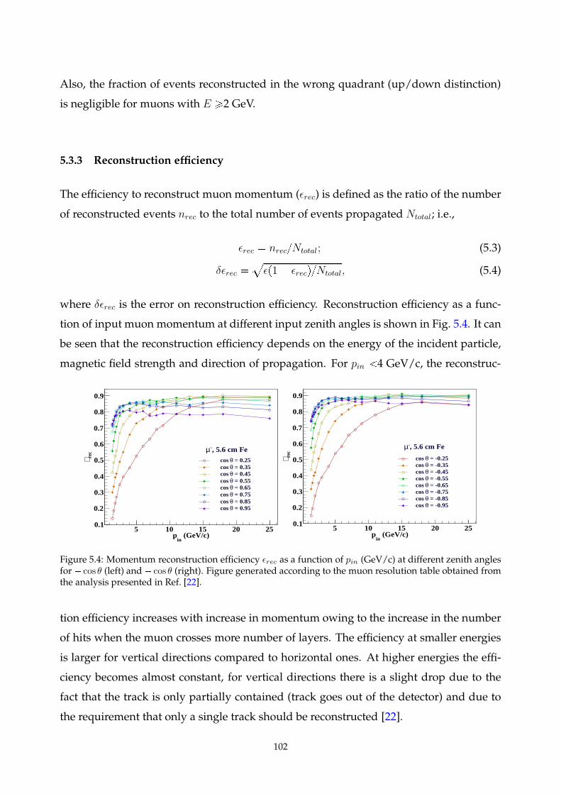
Also, the fraction of events reconstructed in the wrong quadrant (up/down distinction)

is negligible for muons with E ¥2 GeV.

5.3.3 Reconstruction efficiency

The efficiency to reconstruct muon momentum (ǫrec) is defined as the ratio of the number

of reconstructed events nrec to the total number of events propagated Ntotal; i.e.,

ǫrec nrecNtotal; (5.3)

δǫrec a

ǫp1 ǫrecqNtotal, (5.4)

where δǫrec is the error on reconstruction efficiency. Reconstruction efficiency as a func-

tion of input muon momentum at different input zenith angles is shown in Fig. 5.4. It can

be seen that the reconstruction efficiency depends on the energy of the incident particle,

magnetic field strength and direction of propagation. For pin 4 GeV/c, the reconstruc-

(GeV/c)in

p5 10 15 20 25

rec

∈

0.1

0.2

0.3

0.4

0.5

0.6

0.7

0.8

0.9

= 0.25θcos = 0.35θcos = 0.45θcos = 0.55θcos = 0.65θcos = 0.75θcos = 0.85θcos = 0.95θcos

, 5.6 cm Fe-µ

(GeV/c)in

p5 10 15 20 25

rec

∈

0.1

0.2

0.3

0.4

0.5

0.6

0.7

0.8

0.9

= -0.25θcos = -0.35θcos = -0.45θcos = -0.55θcos = -0.65θcos = -0.75θcos = -0.85θcos = -0.95θcos

, 5.6 cm Fe-µ

Figure 5.4: Momentum reconstruction efficiency ǫrec as a function of pin (GeV/c) at different zenith anglesfor cos θ (left) and cos θ (right). Figure generated according to the muon resolution table obtained fromthe analysis presented in Ref. [22].

tion efficiency increases with increase in momentum owing to the increase in the number

of hits when the muon crosses more number of layers. The efficiency at smaller energies

is larger for vertical directions compared to horizontal ones. At higher energies the effi-

ciency becomes almost constant, for vertical directions there is a slight drop due to the

fact that the track is only partially contained (track goes out of the detector) and due to

the requirement that only a single track should be reconstructed [22].

102

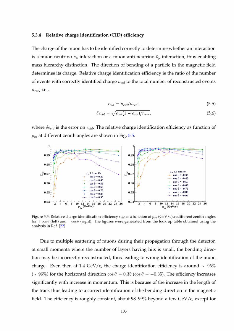
5.3.4 Relative charge identification (CID) efficiency

The charge of the muon has to be identified correctly to determine whether an interaction

is a muon neutrino νµ interaction or a muon anti-neutrino νµ interaction, thus enabling

mass hierarchy distinction. The direction of bending of a particle in the magnetic field

determines its charge. Relative charge identification efficiency is the ratio of the number

of events with correctly identified charge ncid to the total number of reconstructed events

nrec; i.e.,

ǫcid ncidnrec; (5.5)

δǫcid a

ǫcidp1 ǫcidqnrec, (5.6)

where δǫcid is the error on ǫcid. The relative charge identification efficiency as function of

pin at different zenith angles are shown in Fig. 5.5.

(GeV/c)in

p2 4 6 8 10 12 14 16 18 20 22 24 26

cid

∈

0.94

0.95

0.96

0.97

0.98

0.99

1

, 5.6 cm Fe-µ = 0.35θcos = 0.45θcos = 0.55θcos = 0.65θcos = 0.75θcos = 0.85θcos = 0.95θcos

(GeV/c)in

p2 4 6 8 10 12 14 16 18 20 22 24 26

cid

∈

0.94

0.95

0.96

0.97

0.98

0.99

1

, 5.6 cm Fe-µ = -0.35θcos = -0.45θcos = -0.55θcos = -0.65θcos = -0.75θcos = -0.85θcos = -0.95θcos

Figure 5.5: Relative charge identification efficiency ǫcid as a function of pin (GeV/c) at different zenith anglesfor cos θ (left) and cos θ (right). The figures were generated from the look up table obtained using theanalysis in Ref. [22].

Due to multiple scattering of muons during their propagation through the detector,

at small momenta where the number of layers having hits is small, the bending direc-

tion may be incorrectly reconstructed, thus leading to wrong identification of the muon

charge. Even then at 1.4 GeV/c, the charge identification efficiency is around 95%

( 96%) for the horizontal direction cos θ 0.35 (cos θ 0.35). The efficiency increases

significantly with increase in momentum. This is because of the increase in the length of

the track thus leading to a correct identification of the bending direction in the magnetic

field. The efficiency is roughly constant, about 98–99% beyond a few GeV/c, except for

103

the very vertical directions | cos θ| 0.85, 0.95. Even when there is a slight decrease in

ǫcid for these directions, it is does not decrease below 95% in the central region and in

the energy range of interest. Subsequently, a complete analysis of the muon response

over the entire ICAL detector was also performed [108]. The resolutions and results were

marginally worse than those in the central region. While the reconstruction efficiency

was substantially lower, the direction and charge identification efficiencies were similar

to the results in the central region. Thus ICAL has excellent muon charge identification

capability which in turn contributes to the detector’s high sensitivity to neutrino mass

hierarchy.

The values of resolutions and efficiencies were also found out for lower momenta

(pin 1 (GeV/c)) also. These are worse compared to their respective values in the momen-

tum range 1.4 GeV/c and beyond, but it is important to calculate them since the physics

simulation studies consider muon energies down to 0.5 GeV also.

5.4 Separation of charged current muon neutrino events in ICAL

The main interactions of interest in ICAL are the charged current interactions of νµ and

νµ. In addition neutral current interactions of νµ and νµ will also occur in the detector.

Since the atmospheric neutrino flux contains νe and νe also the charged current and neu-

tral current interactions of these neutrinos with the target iron will also take place. Tau

neutrino interactions can also occur in the detector in addition to these but the probabil-

ity of their being a background for charged current muon neutrino events is small. Thus

it becomes important to separate out the channel of interest to study the sensitivity to

neutrino oscillations. Each type of event has its own characteristic signatures which can

be used to identify and tag it. This section describes the preliminary studies on how to

separate different types of events especially charge current muon neutrino events among

the others.

Simulation studies using neutrino events generated using the NUANCE [24] neutrino

generator are conducted in the ICAL detector with default iron plate thickness of 5.6 cm.

The events of interest considered in this study are the charged current and neutral current

interactions of νµ, νµ, νe and νe; ν and ν are taken together and are not distinguished from

each other in this study. The events are named as follows for convenience :

104

1. ccmu : charged current muon neutrino and anti-neutrino events νµ N Ñ µ X ,

νµ N Ñ µ X

2. cce : charged current electron neutrino and anti-neutrino events νe N Ñ e X ,

νe N Ñ e X

3. ncmu : neutral current muon neutrino and anti-neutrino events νµ N Ñ νµ X ,

νµ N Ñ νµ X

4. nce : neutral current electron neutrino and anti-neutrino events νe N Ñ νe X ,

νe N Ñ νe X

Since oscillations have not been turned on, these use no ντ events and the sum of nce and

ncmu will always accurately represent the total neutral current (NC) events.

5.4.1 Separation using strip and layer multiplicity

The primary information available from the RPCs about an event is the hit information.

Since there is no information about the charge deposited by the particles in the detector,

this hit information is used in the separation of different types of events in the ICAL.

The total number of hits in an event along with the number of layers hit in that event

have been used to separate different types of events. This is primarily motivated by the

fact that muons being minimum ionising particles leave long tracks in the detector which

translates to a large number of layers hit in the event. Compared to ccmu events, the other

three events do not traverse so many layers, meaning that long tracks will be absent, but

the hits will be spread widely within a layer. The focus of this section is to make use of

the strip and layer multiplicities of different types of events to identify and tag them.

All the four different types of events were generated in NUANCE neutrino generator

and propagated through the GEANT-4 based ICAL detector. The analysis was done using

unoscillated events. The hit and layer multiplicities of each event was obtained and used

to find out an optimum criterion to identify different types of event. The study was done

using the default plate thickness of 5.6 cm.

105

5.5 Selection criteria based on strip and layer multiplicity

Hit information is the main information available from an event in ICAL. As for the cal-

ibration of hadron energy in Chapter 3, the maximum of the hits in the X plane and Y

plane, the maximum strip multiplicity of the event (s), along with the number of layers

hit in the event (l) are used for this analysis. The 2-dimensional distribution of s and l for

ccmu, cce, ncmu and nce events are shown in Fig. 5.6. It can be seen that the charged cur-

rent muon neutrino (ccmu) events have the maximum number of strips as well as layers

hit. For the other three types of events, the number of strips and layers hit are lesser than

in ccmu events. Hence it is evident from the figure that ccmu events can be separated by

using the number of layers in the event. The number of events having hits in a particular

number of layers in all the different types of events are shown in Fig. 5.7. The number

of layers is large only in the case of ccmu events, and for all the other events, the hits are

confined mostly in less than 10 layers. Only ccmu events have significant amount of

events having hits even in 20 layers. Even though the number of hits is a good criterion

to separate ccmu events, using only this is not tight enough. Hence the idea of using

both l and sl as selection criteria is probed. To set the optimum values for the selection

criteria are set by plotting sl vs l for a fixed l, where s is the total strip multiplicity and

l is the layer multiplicity. This is also illustrated in Fig. 5.7. Several observations can be

made from Fig. 5.7. Only ccmu events have l events beyond 10 layers. The small error

bars for ccmu events indicate the fact that there are significant number of events also. If

an event has more than 4 layers and multiplicity per layer sl ¤ 2, it is a ccmu event

with high probability. Various combination of l and sl were applied to obtain the corre-

sponding recognition efficiencies and sample purities. All events with l 1 and s 1 are

rejected since they cannot be distinguished from noise. Since the events of interest are the

charged current muon neutrino events (ccmu) the selection criteria for those events only

are discussed here. The criteria for identifying other types of events were also studied

but the results were inconclusive and suggestive of the fact that detailed and dedicated

analyses are required to separate those events. This will be discussed elsewhere and is

currently out of the scope of this thesis. The number and fraction of different classes of

events obtained using the criteria l ¥ 5 and sl ¤ 2 are shown in Table 5.1.

About 29% of the ccmu events satisfy the l ¥ 5 criterion, while only less than 4%

of the other three types of events, i.e., cce, ncmu and nce satisfy this criterion. This means

106

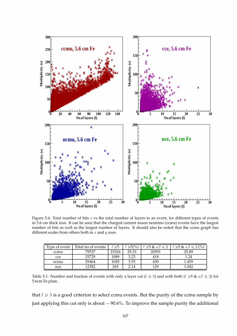
No.of layers (l)0 20 40 60 80 100 120 140

Mu

ltip

licity (

s)

0

50

100

150

200

250

300

ccmuEntries 70609Mean x 6.448Mean y 10.25RMS x 11.99RMS y 16.58

ccmuEntries 70609Mean x 6.448Mean y 10.25RMS x 11.99RMS y 16.58

ccmu, 5.6 cm Fe

No.of layers (l)0 5 10 15 20 25 30

Mu

ltip

licity (

s)

0

50

100

150

200cce

Entries 29794Mean x 2.003Mean y 6.217RMS x 1.237RMS y 7.361

cceEntries 29794Mean x 2.003Mean y 6.217RMS x 1.237RMS y 7.361

cce, 5.6 cm Fe

No.of layers (l)0 5 10 15 20 25 30

Mu

ltip

licity (

s)

0

50

100

150

200

ncmuEntries 21473Mean x 1.902Mean y 4.613RMS x 1.489RMS y 7.155

ncmuEntries 21473Mean x 1.902Mean y 4.613RMS x 1.489RMS y 7.155

ncmu, 5.6 cm Fe

No.of layers (l)0 5 10 15 20 25 30

Mu

ltip

licity (

s)

0

50

100

150

200

nceEntries 8882Mean x 1.765Mean y 3.997RMS x 1.165RMS y 5.135

nceEntries 8882Mean x 1.765Mean y 3.997RMS x 1.165RMS y 5.135

nce, 5.6 cm Fe

Figure 5.6: Total number of hits s vs the total number of layers in an event, for different types of eventsin 5.6 cm thick iron. It can be seen that the charged current muon neutrino (ccmu) events have the largestnumber of hits as well as the largest number of layers. It should also be noted that the ccmu graph hasdifferent scales from others both in x and y axes.

Type of event Total no.of events l ¥5 l ¥5(%) l ¥5 & sl ¤ 2 l ¥5 & sl ¤ 2 (%)ccmu 79537 23326 29.33 20591 25.89cce 33729 1089 3.23 418 1.24

ncmu 29464 1045 3.55 430 1.459nce 12382 265 2.14 129 1.042

Table 5.1: Number and fraction of events with only a layer cut (l ¥ 5) and with both (l ¥5 & sl ¤ 2) for5.6cm Fe plate.

that l ¥ 5 is a good criterion to select ccmu events. But the purity of the ccmu sample by

just applying this cut only is about 90.6%. To improve the sample purity the additional

107

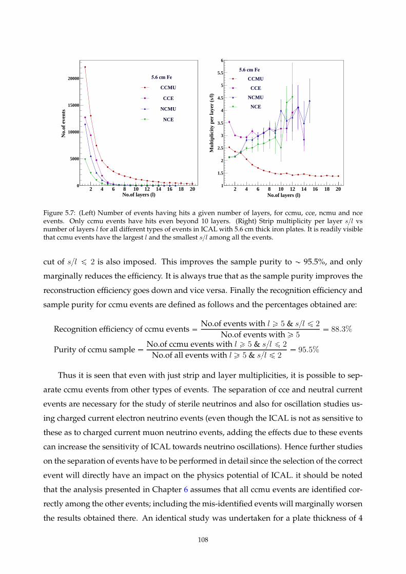
No.of layers (l)2 4 6 8 10 12 14 16 18 20

No.

of e

vent

s

0

5000

10000

15000

20000 5.6 cm Fe

CCMU

CCE

NCMU

NCE

No.of layers (l)2 4 6 8 10 12 14 16 18 20

Mul

tiplic

ity p

er la

yer

(s/l)

1

1.5

2

2.5

3

3.5

4

4.5

5

5.5

6

5.6 cm Fe

CCMU

CCE

NCMU

NCE

Figure 5.7: (Left) Number of events having hits a given number of layers, for ccmu, cce, ncmu and nceevents. Only ccmu events have hits even beyond 10 layers. (Right) Strip multiplicity per layer sl vsnumber of layers l for all different types of events in ICAL with 5.6 cm thick iron plates. It is readily visiblethat ccmu events have the largest l and the smallest sl among all the events.

cut of sl ¤ 2 is also imposed. This improves the sample purity to 95.5%, and only

marginally reduces the efficiency. It is always true that as the sample purity improves the

reconstruction efficiency goes down and vice versa. Finally the recognition efficiency and

sample purity for ccmu events are defined as follows and the percentages obtained are:

Recognition efficiency of ccmu events No.of events with l ¥ 5 & sl ¤ 2

No.of events with ¥ 5 88.3%

Purity of ccmu sample No.of ccmu events with l ¥ 5 & sl ¤ 2

No.of all events with l ¥ 5 & sl ¤ 2 95.5%

Thus it is seen that even with just strip and layer multiplicities, it is possible to sep-

arate ccmu events from other types of events. The separation of cce and neutral current

events are necessary for the study of sterile neutrinos and also for oscillation studies us-

ing charged current electron neutrino events (even though the ICAL is not as sensitive to

these as to charged current muon neutrino events, adding the effects due to these events

can increase the sensitivity of ICAL towards neutrino oscillations). Hence further studies

on the separation of events have to be performed in detail since the selection of the correct

event will directly have an impact on the physics potential of ICAL. it should be noted

that the analysis presented in Chapter 6 assumes that all ccmu events are identified cor-

rectly among the other events; including the mis-identified events will marginally worsen

the results obtained there. An identical study was undertaken for a plate thickness of 4

108

cm; a similar behaviour was observed.

5.6 Chapter Summary

The main interactions of interest in the ICAL are the charged current interaction of νµ and

νµ with the iron target. The muons produced in the final state of these interactions, being

minimum ionising particles, leave long clean tracks in the detector unlike the hadrons

which shower. These tracks are bent in the magnetic field of the detector and the direc-

tion of the bending makes it possible to identify the charge of the muon. The momentum

and direction of the muon can be reconstructed using a Kalman filter algorithm. The

momentum and direction resolution, and the reconstruction efficiencies and charge iden-

tification efficiencies for muons in the central region of each module where the magnetic

field is uniform have been estimated elsewhere [22] using a GEANT-4 based simulation

studies. The results of this study have been collated for use in Chapter 6. It is seen that

the muons have excellent momentum and direction resolution in the ICAL as compared

to the hadrons. The charge identification efficiency for muons is always more than 95%

indicating that ICAL is very well optimised for muon detection.

The separation of different types of events in ICAL is also very important. Muons

are easily identifiable with their long tracks and lower strip multiplicity whereas the sep-

aration of neutral current events from charged current electron events is rather difficult

due to the presence of showers in these events. This is studied using simulations by

propagating the particles produced from each type of events, generated using NUANCE.

Selection criteria based on strip and layer multiplicities of an event are implemented to

separate the different types of events from one another. It is seen that most of the charged

current muon neutrino events can be identified easily with the large number of layers and

lesser strip multiplicity per layer owing to the presence of the minimum ionising muon

in the event. However further studies on the separation of the other three types of events

namely cce, ncmu and nce have to be done in detail to extract as much information from

these events as possible. Both the separation of various types of particles (events) in the

ICAL and quantifying their energy and direction resolutions is necessary to be used as

inputs to the oscillation physics analysis with ICAL. Any improvement in the efficiencies

and resolutions is crucial with respect to the physics potential of ICAL and simulations

will throw light on these.

109

Part III

Simulation studies of the sensitivities of the ICAL detectorto neutrino oscillation parameters

6

Precision measurements of θ23 and

|∆m232| and mass hierarchy sensitiv-

ity of ICAL in the context of adding

higher muon energy bins and con-

straining the neutrino-antineutrino

flux ratio6.1 Overview

The iron calorimeter detector (ICAL) at INOwill be a magnetised iron calorimeter mainly

sensitive to the interaction of atmospheric neutrinos with the iron target in the detector.

The main physics goals of ICAL include probing the earth matter effect on the propaga-

tion of atmospheric neutrinos and hence resolve the mass hierarchy puzzle, i.e., the sign

of ∆m232 where ∆m2

32 m23 m2

2,m2, m3 being the mass eigenstates of neutrinos.

ICALwill actually probe the mass ordering in the 2–3 sector, i.e., it will determine the

sign of∆m232. The determination of the mass hierarchy also requires knowledge of the ab-

solute scale of neutrino masses. These can only be probed in direct detection experiments

such as tritium beta decay [136–139] or in neutrinoless double beta decay [140–144]. It is

noted that if the lowest mass eigenstate is relatively heavy, all the mass eigenstates are

degenerate and roughly of the order of 0.1 eV, i.e., about one third of the limit on the sum

of the neutrino masses arising from cosmological observations [145, 146]. On the other

hand, if the lightest neutrino is nearly massless, the observed neutrino mass ordering will

also determine the hierarchy. In this Chapter, mass ordering and hierarchy are referred to

interchangeably.

ICAL will not only determine the 2–3 neutrino mass ordering, but will also perform

precision measurements of the atmospheric mixing angle θ23 and mass squared differ-

ence ∆m232. This precision measurement will in turn contribute to improving the current

precision limits set by MINOS [33] and T2K [147]. MINOS is also a magnetised detector,

but it is only 5400 tons whereas ICAL will be 50 ktons in mass which will impact ICAL’s

physics reach. Magnetisation will help ICAL in distinguishing neutrino events from anti-

neutrino events, by means of having an excellent charge identification efficiency. This

distinction improves the sensitivities of ICAL to oscillation parameters. Thus unlike wa-

ter cherenkov detectors like Super-K [78], ICALwill be able to do precision measurements

very well and also determine the neutrino mass ordering efficiently.

The source of neutrinos in ICAL are naturally occuring neutrinos produced over

a range of few GeVs to a few 100 GeVs (sub GeV to multi GeV) in the upper atmo-

sphere when primary cosmic ray particles (mainly protons) interact with the nuclei there

[113, 117]. These neutrinos while passing through the Earth undergo oscillations and the

neutrinos which interact with the iron target carry the signatures of oscillations. Since real

data is not available, simulation studies have been carried out to study the sensitivities

of ICAL detector to atmospheric oscillation paratmeters. The main steps involved in this

are neutrino event generation, inclusion of detector responses and efficiencies, inclusion

of oscillations, binning in observables and χ2 analysis. The analysis is discussed in detail

in the following sections. This work will also be reported in Ref. [35].

6.2 Neutrino events generation

NUANCE neutrino event generator (version 3.5) [24] is used to generate the required

interactions of atmospheric neutrinos in ICAL. Atmospheric neutrino flux at the Super

Kamiokande site, as provided by Honda et al. [117] is used to generate the events. The

energy range of the generated neutrinos is 0.4 – 500 GeV. The composition of ICAL de-

tector (mainly RPC glass and iron) is fed into NUANCE as input. NUANCE generates

all possible interactions for all neutrino flavours in different materials which constitute

the detector, by knowing the the differential cross sections for different types of inter-

actions. Both charged current (CC) and neutral current (NC) interactions are generated,

and the different classes in each channel include quasi-elastic (QE), resonance (RES), deep

inelastic (DIS), coherent scattering (CO) and diffractive scattering (DF). The event rates

for all scattering processes with the target nuclei are calculated by multiplying neutrino

fluxes read from Honda flux tables with the interaction cross sections. The kinematics of

each event is generated depending upon the flux and differential cross section. The out-

put of NUANCE consists of particle id number (pid), interaction process id, information

whether a particle belongs to the initial, intermediate and final state, four-momentum

113

(pµ) of the initial and final state particles, interaction vertex and time of interaction of the

particles. For the purpose of physics analysis (and as input to GEANT-4 simulation code

for ICAL), only the information about particle id, interaction vertex, four momentum and

time are retained. Particle ids of the initial and final state particles are important to deter-

mine whether the interaction is charged current or neutral current. Also pid is important

to determine whether the interaction is that of a neutrino or anti-neutrino ; this along with

the four-momentum information of the neutrino is used to call the appropriate oscillation

probabilities while applying oscillations on each events. Four-momentum information is

required to determine the true energy and direction of the final state particles which will

further be used to determine the bins to which these events belong to and to smear these

values accordingly. Even though the analyses are done for a smaller number of years (say

5, 10, 15, 20), NUANCE data sample for exactly these years are not generated. Instead

a huge data sample for a very large number of years (here 1000 years) is generated and

scaled down to the required number of years during the analysis. This is mainly done

to reduce the effect of statistical (Monte Carlo) fluctuations on sensitivity studies, which

may alter the results. A detailed discussion about the effect of fluctuations on oscillation

sensitivity studies will be discussed in section 6.10.

6.3 Oscillation probabilities

The oscillation probabilities calculated by considering full three flavour oscillations in the

presence of matter effects, as discussed in Section 1.4.1 are used for the analysis. The Pre-

liminary Reference Earth Model (PREM) profile [148] has been used to model the varying

Earth matter density encountered by the neutrinos during their travel through the Earth.

For the precise measurement of the oscillation parameters, the neutrino oscillation proba-

bilities in matter can be calculated to a high degree of accuracy using numerical methods.

The Runge-Kutta solver method is used to calculate the oscillation probabilities for var-

ious energies E and distances L/or equivalently cos θ (θ being the zenith angle). The

results obtained in the analyses presented in the following sections make use of the evo-

lution of flavour eigenstates through Earth’s varying matter density as described by the

PREM profile. The PREM profile as a function of the radius r from the center of the Earth

is shown in Fig. 6.1. The discontinuity at the inner-outer core as well as the core-mantle

transitions can also be seen. An up-going neutrino which is of interest in atmospheric

114

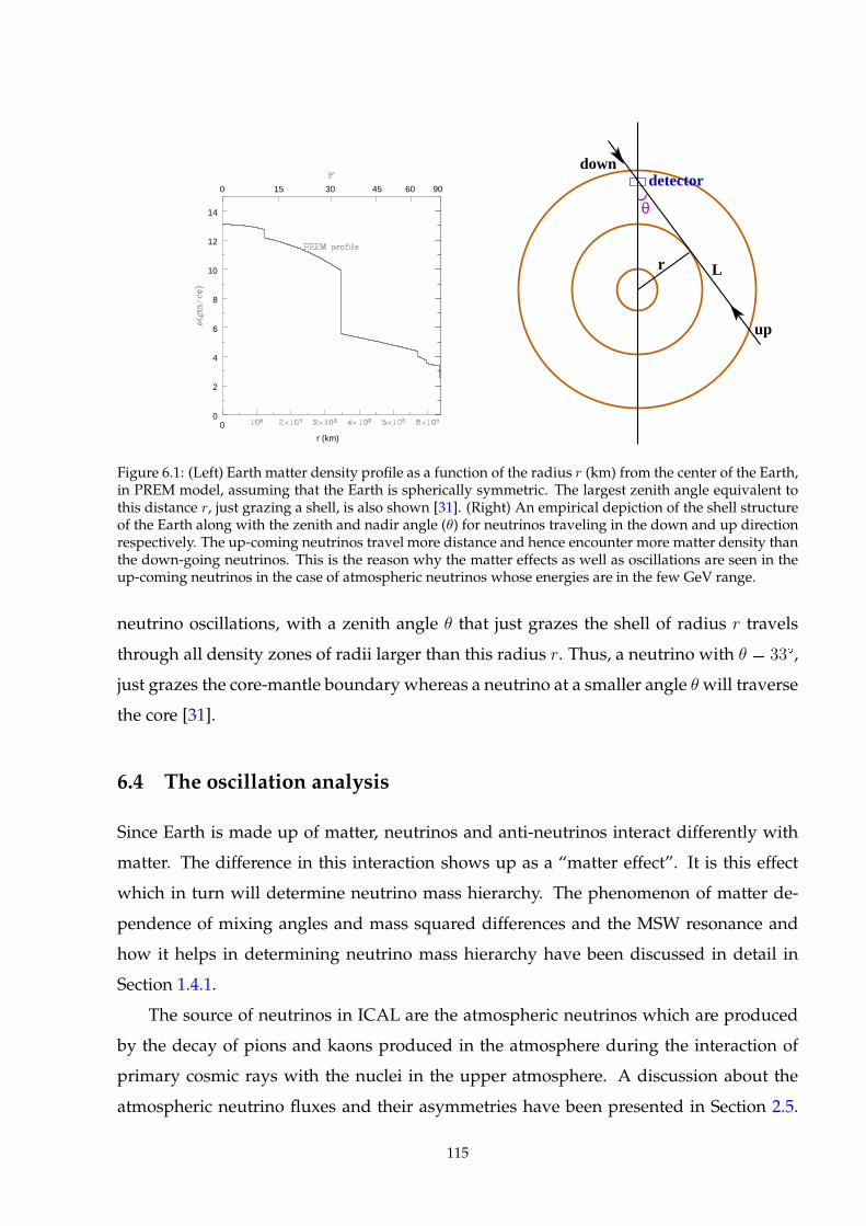
00

2

4

6

8

10

12

14

r (km)

0 15 30 45 60 90

θ

r L

up

downdetector

Figure 6.1: (Left) Earth matter density profile as a function of the radius r (km) from the center of the Earth,in PREM model, assuming that the Earth is spherically symmetric. The largest zenith angle equivalent tothis distance r, just grazing a shell, is also shown [31]. (Right) An empirical depiction of the shell structureof the Earth along with the zenith and nadir angle (θ) for neutrinos traveling in the down and up directionrespectively. The up-coming neutrinos travel more distance and hence encounter more matter density thanthe down-going neutrinos. This is the reason why the matter effects as well as oscillations are seen in theup-coming neutrinos in the case of atmospheric neutrinos whose energies are in the few GeV range.

neutrino oscillations, with a zenith angle θ that just grazes the shell of radius r travels

through all density zones of radii larger than this radius r. Thus, a neutrino with θ 33,

just grazes the core-mantle boundary whereas a neutrino at a smaller angle θwill traverse

the core [31].

6.4 The oscillation analysis

Since Earth is made up of matter, neutrinos and anti-neutrinos interact differently with

matter. The difference in this interaction shows up as a “matter effect”. It is this effect

which in turn will determine neutrino mass hierarchy. The phenomenon of matter de-

pendence of mixing angles and mass squared differences and the MSW resonance and

how it helps in determining neutrino mass hierarchy have been discussed in detail in

Section 1.4.1.

The source of neutrinos in ICAL are the atmospheric neutrinos which are produced

by the decay of pions and kaons produced in the atmosphere during the interaction of

primary cosmic rays with the nuclei in the upper atmosphere. A discussion about the

atmospheric neutrino fluxes and their asymmetries have been presented in Section 2.5.

115

The atmospheric neutrino flux used for the analyses presented here are the Honda-3D

fluxes at the Kamioka site. The fluxes at Theni where INO will be located are marginally

different, especially they are smaller at lower energies. These fluxes are just being made

available and hence is beyond the scope of this thesis.

6.4.1 Total number of neutrino events for a given exposure time

The interactions of interest in ICAL are the charged current interactions of νµ and νµ with

the iron target in ICAL. These νµ (νµ) in ICAL come from both νµ and νe atmospheric

fluxes via νµ Ñ νµ and νe Ñ νµ oscillations. The first channel gives the number of νµ

events which have survived and the second one gives the number from oscillations of νe

to νµ. The number of events ICAL sees will be a sum of these events. Thus,

d2N

dEµ d cos θµν

t nd

»

dEν d cos θν dφν

Pµµd3Φνµ

dEν d cos θν dφν Peµ

d3ΦνedEν d cos θν dφν

dσνµpEνq

dEµ d cos θµν,

(6.1)

where, t is the exposure time, nd is the number of targets in the detector, σνµ is the differ-

ential neutrino interaction cross section in terms of the energy and opening angle of the

CC lepton, Φνµ andΦνe = νe are the νµ and νe fluxes and Pαβ is the oscillation probability of

να Ñ νβ. The number of events in a bin of (Eµ, cos θµν) is obtained by integrating over the

bin, Before doing this, the final state variables are transformed to (Eµ, cos θµ) so that the

events are binned in the observable polar angle of the muon rather than the unobservable

θµν , the opening angle of the muon with respect to the neutrino. These transformations

are performed within NUANCE and the output of NUANCE lists events as discussed

earlier. These are taken and binned accordingly.

The expression in Eq. 6.1 is for the ideal case when the detector has perfect resolu-

tions and 100% efficiencies. To get the actual number of events, realistic resolutions and

efficiencies obtained from GEANT-4 based simulation studies of ICAL have to be incor-

porated as discussed in the following sections.

116

6.5 Inclusion of detector responses and efficiencies

Every detector has its own resolution with which it can distinguish different energies and

directions. The efficiencies with which the final state particles can be detected are also

important and affect the calculation of no.of oscillated events. The energy and direction

resolutions of muons, to the detection of which the detector is optimised is excellent [22].

Hadrons which are also produced in the charged current interactions have worse energy

and direction resolutions [20]. Even then the inclusion of hadron information has proved

to enhance ICAL sensitivities [27]. These resolutions and efficiencies have been tabulated

and these tables are used to smear the true energies of the final state particles (muons and

summed hadrons) to the values that will be seen in the detector and used in the analy-

sis. It should be noted that muon resolutions and efficiencies vary in different regions

of the detector according to the strength and direction of magnetic field [22, 108]. This

analysis uses the responses and efficiencies of muons in the central region of the detector,

discussed in Chapter 5. These are the best of all possible muon responses in the ICAL

detector. While the energy and direction resolutions of muons as well as their charge

identification efficiency is similar in the peripheral regions, the reconstruction efficiency

is smaller because of edge effects including smaller magnetic field. Hence including the

entire volume of ICAL will marginally reduce the total number of events for a given ex-

posure time – the consequences of this reduction have not been discussed in this thesis.

In addition to muon momentum and direction, the energy of the multiple hadrons pro-

duced in ICAL are used as observables in the analysis. Since hadrons traverse relatively

few layers, the results on hadron energy resolutions obtained in Chapter 3 in the cen-

tral region of ICAL apply over entire ICAL without much impact due to edge effects etc.

Hence the energy resolutions of multiple hadrons propagating in the central part of the

detector, which were estimated using GEANT-4 based simulation studies[20] are used.

These realistic values obtained from simulating the propagation of muons and hadrons

in ICAL simulated using GEANT-4 have been used in the analysis presented here.

6.5.1 Smearing of energies and direction: inclusion of detector resolutions

At the time this calculation was begun, the responses of both muons and hadrons in the

peripheral parts of ICAL was not completely understood. Hence, instead of propagating

the NUANCE events through the simulated ICAL detector in GEANT and obtaining a

117

more realistic set of “observed” values of the energy and momentum of the final state

particles, the true values of these variables were smeared according to the resolutions

obtained in the earlier studies using random number generators. Subsequently, the pe-

ripheral regions of ICAL have also been well understood. However, the extension of the

study to perform a full GEANT4-based analysis is beyond the scope of this work.

In the analysis, the energy and direction of muons and energy of hadrons in the final

state of interaction have been used as observables. The reconstructed values of these

observables will depend on detector resolutions. The better the detector resolution, the

closer will be the observed value to the true value. To take into account the fact that the

detector has a certain resolution, the true values are smeared using the look up tables

prepared from ICAL GEANT4 simulations.

6.5.1.1 Smearing of muon momentum and direction

The muon look up table lists the mean and σ of the reconstructed distribution obtained

from simulations of fixed energy muons for fixed true values of pEiµ, cos θ

jµq as well as the

reconstruction and CID efficiencies in those bins. For each NUANCE event, a uniform

random number generator is used to generate the smeared/observed value of each of

Eµ, cos θµ with a probability consistent with the distribution in the table whose pEiµ, cos θ

jµq

corresponds closest to the true pEµ, cos θµq of that event. While the smeared values of Eµ

and cos θµ are henceforth used in place of the original values, the information on recon-

struction and CID efficiencies (again taken from the look-up table) is retained for each

event for later use.

In the case of muon energy and direction, the smearing is done consistent with the

Gaussian distribution function using the true particle energyEµ obtained from NUANCE

as the mean and σ of the nearest Eiµ from the look-up table as the width. Only positive

values of smeared energy Eobsµ are allowed; if the smeared energy happens to be negative,

the random number is called repeatedly till a positive value is obtained. A smeared cos θµ

value is obtained in a similar fashion. Since the allowed range of cos θ is from r1,1s

only, for cases when the smeared value of cos θobsµ 1 and cos θobsµ ¡ 1, the conditions

cos θobsµ 1 and cos θobsµ 1 are imposed so as to confine the smeared values of

cos θobsµ also in the allowed range r1,1s. This is preferred to wrapping the cos θ ¡ 1

values back into the correct range since the distributions are very narrow in cos θ (σ 1).

118

In the case of hadrons, the smearing is not done directly. Momentum of muons can be

measured directly in ICAL by using curvature method (using Kalman filter technique).

But in the case of hadrons, energy is calibrated to the number of hits in the hadron shower.

Hence the smearing of hadron cannot be done directly, but only by smearing the number

of hits and recalibrating them to energy. A brief description of hadron energy smearing

is given here.

6.5.1.2 Hadron energy smearing

First the true energy of the hadrons produced in a charged current muon neutrino in-

teraction is determined as E 1truehad Etrue

ν Etrueµ , where Etrue

ν is the true energy of the

incident neutrino and Etrueµ is the true energy of the final state muon. This true hadron

energy is binned into a true hadron energy bin. If E 1truehad 1 GeV, then the energy is taken

to be Eobshad 0 GeV. If E 1true

had ¥ 1 GeV, the hadron look up table is used and the Vav-

ilov parameters corresponding to the true energy bins are read and used to implement

smearing via Vavilov distribution function. The smearing is indirect since the number of

hits corresponding to the true bin is generated from these parameters and the energy is

then calibrated to the number of hits. To generate such a hit distribution, the following

procedure is adopted. Let the mean number of hits calculated from Vavilov parameters

for a given E 1truehad which is the central bin value (from hadron look-up table) be:

meanvav pγ 1 lnP0 P1qP3 P2 xN P2, (6.2)

where γ 0.57721 (Euler’s constant) and Pi, with i 0, 1, 2, 3 are Vavilov parameters as

described in Section. A.0.1. This equation generates the mean number of hits in the given

true hadron energy bin. However, the hadron energy of the actual event may not be the

same as the bin centre. Hence to generate the mean number of hits corresponding to a

given true hadron energy, a linear approximation of the number of hits to the true hadron

energy is used :

nt n0

h E 1truehad n1h, (6.3)

where, n0

h = 1.6 is the slope and n1h = 5.7, the intercept of the linear fit. Thus, for the

true hadron energy E 1truehad , the mean number of hits corresponding to this particular en-

ergy is given by nt and the Vavilov distribution is thus rescaled to have this mean value.

That is the shifted Vavilov distribution has P 1

2 nt xN , where P 1

2 is the modified P2,

119

xN pγ 1 lnP0 P1qP3. This P1

2 is used to generate hits distributed according to a

Vavilov distribution, distributed about the shifted mean :

vdis pvinv P3q P 1

2, (6.4)

where vinv is a Vavilov random number with P0 and P1 as κ and β2 respectively. Now

the smeared hits are calibrated back to energy using the expression :

E 1obshad

vdis n1hn0

h

. (6.5)

. If the smeared value of energy happens to be negative, i.e., if E 1obshad 0, a new random

number is generated and the whole process is repeated as in the case of muon energy

smearing until a positive value is obtained.

6.5.2 Applying neutrino oscillations

A sample of 1000 years of unoscillated data was generated using NUANCE. Two data

sets were generated :

1. CC muon events using the Φµ flux and

2. CC muon events using the swapped Φe Ñ Φµ flux.

This generates the so-called muon- and swapped-muon events that corresponds to the

two terms in Eq. 6.1. Oscillations were then applied in two different ways. In the first

study, the Pµµ (or Pµµ) was calculated given the pEν , cos θνq of the event. A random num-

ber r was generated. If Pµµ ¡ r, then the event was retained; else it was dropped. A

similar procedure was carried out for the swapped events with respect to Peµ (and for

anti-neutrinos as well). The surviving events were then binned in the appropriate ob-

served bins for analysis.

In the second approach which was finally used in the analysis, the generated event

was simply multiplied by Pµµ (or Peµ) and then binned. This procedure gave similar

results to the first one for the thousand year data with a 10 year data set, however the first

approach gave rise to random fluctuations (as expected) which gave appreciably different

data sets on each iteration. As discussed in [27], using the first approach generates the

statistical mean distribution with respect to which an unbiased analysis can be performed.

120

The oscillation is applied event by event (for both muon and swapped muon events)

and it is a time consuming process since the actual sample contains 1000 years of data.

6.5.3 Binning in observed energies and direction

It is always in terms of observables that the analysis is done. It is because of this that

the energies and direction of the final state particles had to be smeared according to de-

tector resolutions. The observables used in the analysis discussed here are muon energy

Eobsµ , muon direction cos θobsµ and hadron energy E 1obs

had . There are two different binning

schemes, one inwhich only themuon energy and direction are used, i.e., the pEobsµ , cos θobsµ q

called the 2D (mu only) binning scheme and the other in which all the three observ-

ables pEobsµ , cos θobsµ , E 1obs

had q are used, which is also known as the 3D (with hadron) binning

scheme. Previous analyses of ICAL physics [27, 29, 30], were done in the observed muon

energy range of Eobsµ = 0.8 – 10.8 GeV and 1 – 11 GeV (both being approximately same).

The analysis discussed here takes into consideration, the extended energy region of the

observed muon energy Eobsµ = 0.5 – 25 GeV. Even though this includes the lower energy

region which contains larger neutrino flux, it will be seen that it is the inclusion of the

higher energy bins beyond 11 GeV, which contributes to the improved results discussed

in Section. 6.6. The motivation to use the extended energy range of the observed muon

energy can be justified from Fig. 6.2 where the number of νµ and νµ events in various

logpLobsµ Eobsµ q bins, where Lobsµ is the observed muon path length and Eobs

µ is the observed

muon energy are shown. The events are calculated after applying oscillation probabilities

(using the central values of oscillation parameters) and detector efficiencies in each bin.

The comparison of the number of events in different logpLobsµ Eobsµ q bins when Eobs

µ is 1–11

GeV only and with Eobsµ extended to 0.5–25 GeV, for νµ and νµ are shown in the figure.

[Roughly speaking, the left peak corresponds to down-going events and the right one to

up-coming events.] It can be seen that the with the extension of the energy range, a larger

range of logpLobsµ Eobsµ q is spanned, which increases the sensitivities to oscillation param-

eters. The number of events also increases with the extension of the energy range, again

giving a better sensitivity to oscillation parameters. It should be noted that the binning in

logpLobsµ Eobsµ q is used for representational purposes only. For the actual analysis separate

bins of Eobsµ and cos θobsµ along with E 1obs

had are used as described below.

The binning scheme is discussed now. As mentioned earlier, there are two binning

121

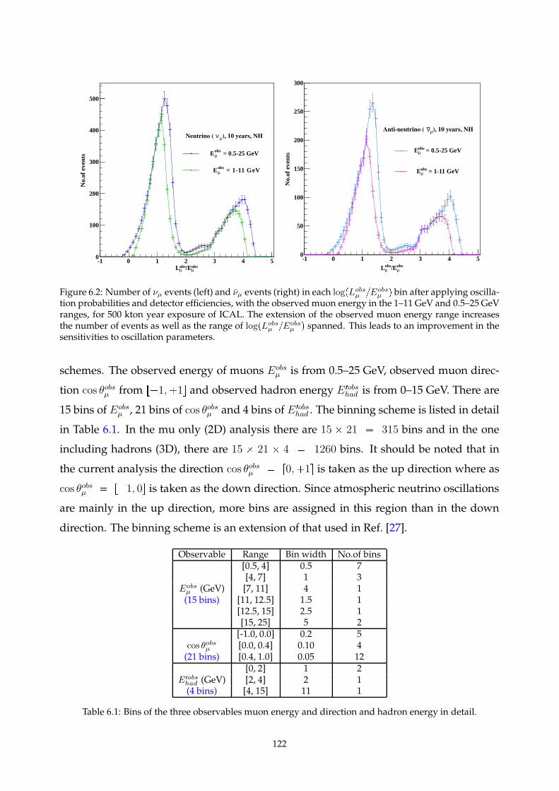
µobs/Eµ

obsL-1 0 1 2 3 4 5

No.

of e

vent

s

0

100

200

300

400

500

), 10 years, NHµνNeutrino (

= 0.5-25 GeVµobsE

= 1-11 GeVµobsE

µobs/Eµ

obsL-1 0 1 2 3 4 5

No.

of e

vent

s

0

50

100

150

200

250

300

), 10 years, NHµνAntineutrino (

= 0.5-25 GeVµobsE

= 1-11 GeVµobsE

Figure 6.2: Number of νµ events (left) and νµ events (right) in each logpLobsµ Eobs

µ q bin after applying oscilla-tion probabilities and detector efficiencies, with the observedmuon energy in the 1–11 GeV and 0.5–25 GeVranges, for 500 kton year exposure of ICAL. The extension of the observed muon energy range increasesthe number of events as well as the range of logpLobs

µ Eobsµ q spanned. This leads to an improvement in the

sensitivities to oscillation parameters.

schemes. The observed energy of muons Eobsµ is from 0.5–25 GeV, observed muon direc-

tion cos θobsµ from r1,1s and observed hadron energy E 1obshad is from 0–15 GeV. There are

15 bins of Eobsµ , 21 bins of cos θobsµ and 4 bins of E 1obs

had . The binning scheme is listed in detail

in Table 6.1. In the mu only (2D) analysis there are 15 21 315 bins and in the one

including hadrons (3D), there are 15 21 4 1260 bins. It should be noted that in

the current analysis the direction cos θobsµ r0,1s is taken as the up direction where as

cos θobsµ r1, 0s is taken as the down direction. Since atmospheric neutrino oscillations

are mainly in the up direction, more bins are assigned in this region than in the down

direction. The binning scheme is an extension of that used in Ref. [27].

Observable Range Bin width No.of bins[0.5, 4] 0.5 7[4, 7] 1 3

Eobsµ (GeV) [7, 11] 4 1(15 bins) [11, 12.5] 1.5 1

[12.5, 15] 2.5 1[15, 25] 5 2[-1.0, 0.0] 0.2 5

cos θobsµ [0.0, 0.4] 0.10 4(21 bins) [0.4, 1.0] 0.05 12

[0, 2] 1 2E1obs

had (GeV) [2, 4] 2 1(4 bins) [4, 15] 11 1

Table 6.1: Bins of the three observables muon energy and direction and hadron energy in detail.

122

6.5.4 Detection efficiencies and number of events

Every detector has a certain value of detection efficiency for each particle with a given

energy and traveling in a given direction. Thus out of a given sample only a certain

fraction will be reconstructed at a given energy and in a given direction. This is called

reconstruction efficiency ǫr. The values of ǫr for each true energy and cos θ bins for muons

are read from the look up table and used in the analysis. Here, reconstruction efficiency of

an event is taken to be the ability to see a muon, that is to be able to reconstruct it. Hence

when hadron energy is added as the third observable, the efficiency in detecting an event

remains the same.

The main characteristic of ICALwhich makes it a special detector and suited for mass

hierarchy determination is its ability to distinguish between neutrino and anti-neutrino

events by separating muons from anti-muons by means of a magnetic field. Thus it iden-

tifies the charge of the final state muons using a magnetic field. The ability of the detector

to identify events of a particular charge is known as charge identification ǫcid efficiency. This

is incorporated to calculate the number of νµ and νµ events separately. First the number

of events in the 2D binning scheme can be found out. The total number of νµ events in

each bin will be a sum of νµ events correctly identified as νµ events and νµ events wrongly

identified as νµ events. Thus charge identification efficiency comes into play in determin-

ing the number of events per bin. Similarly, the number of νµ events in each bin is the

sum of correctly identified νµ events and νµ events wrongly identified as νµ events. The

number of events per bin depends on the reconstruction efficiency in each bin. This is

also taken into account while determining the number of events per bin. Thus,

N totµpE

obsµ , cos θobsµ q Nµǫrecǫcid Nµǫrecp1 ǫcidq, (6.6)

N totµpE

obsµ , cos θobsµ q Nµǫrecǫcid Nµǫrecp1 ǫcidq, (6.7)

(6.8)

where, N totµ

(N totµ

) is the total number of νµ (νµ) CC muon events in the bin pEobsµ , cos θobsµ q,

Nµ and Nµ are the number of events in this bin for an ideal detector with 100% recon-

struction and CID efficiencies. The quantity ǫrec is the reconstruction efficiency of muons

with a given energy and direction and ǫcid is the charge identification efficiency of the

same. The reconstruction and charge identification efficiencies for µ and µ have been

123

taken to be the same. It is straightforward to include unequal values fro them, but the

studies show that they are only marginally different in a few energy-cos θ bins. Finally,

the events in a bin are considered non-zero if there is at least one event in that bin. This

procedure is used both N are the data events D and theory events T .

The number of oscillated events in the bin observed bin pEobsµ , cos θobsµ q is given by:

Noscµ Nµ Pαβ, (6.9)

Noscµ Nµ Pαβ, (6.10)

where Pαβ is the probability of oscillation from a neutrino flavour να to a neutrino flavour

νβ and Pαβ is the probability of oscillation from an anti-neutrino flavour να to a flavour

νβ; α, β are µ, µ and e, µ.

These events are used for the physics analysis. Now this 1000 year data sample is

scaled to the same number of years as the data, for comparison and calculation of χ2. The

current precision analysis is done for 10 years of exposure of 50 kton ICAL (500 kton year).

For the χ2 analysis, the oscillation parameters are changed and the aforementioned pro-

cesses are repeated. This new data is called ”theory“ and different theories are generated

by changing the oscillation parameters.

6.6 χ2 analysis

The χ2 analysis is done in the observed bins discussed in Section 6.5.3. Since neutrino

experiments are low counting events, Poissonian χ2 is used in the analysis. There are two

χ2 analyses here; one with 10 systematic pulls and the other with 11 pulls. In the former,

χ2s from neutrino events and anti- neutrino events are uncorrelated and can be defined

separately and summed. In the case of the latter, a 11th pull is added as a constraint on

the neutrino anti-neutrino flux ratio, hence there are no separate χ2s for these events.

Analyses are done for both 2D and 3D binning schemes, but the expressions are similar

except for the bins. The expression for χ2 for the 10 pulls case is :

124

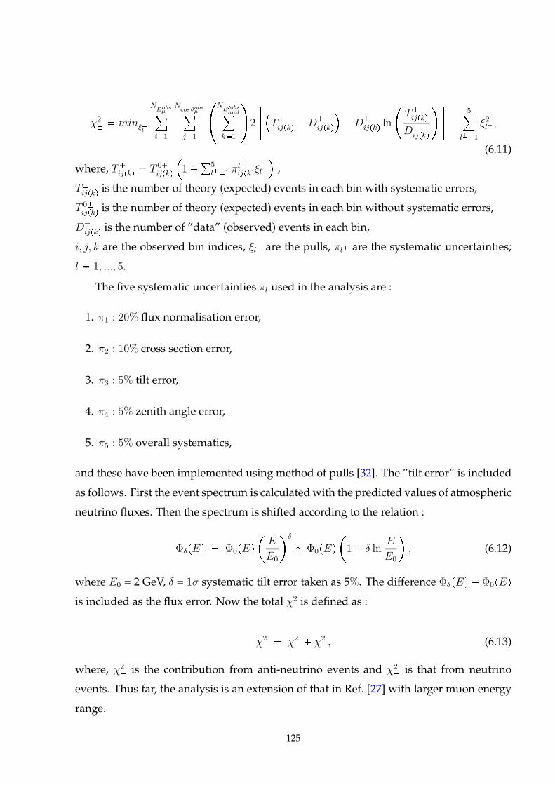
χ2

minξl

NEobsµ¸

i1

Ncos θobsµ¸

j1

NE1obshad¸

k1

2

T

ijpkqD

ijpkq

D

ijpkqln

T

ijpkq

D

ijpkq

5¸

l1

ξ2l,

(6.11)

where, T

ijpkq T 0

ijpkq

1°

5

l1πl

ijpkqξl

,

T

ijpkqis the number of theory (expected) events in each bin with systematic errors,

T 0

ijpkqis the number of theory (expected) events in each bin without systematic errors,

D

ijpkqis the number of ”data” (observed) events in each bin,

i, j, k are the observed bin indices, ξl are the pulls, πl are the systematic uncertainties;

l 1, ..., 5.

The five systematic uncertainties πl used in the analysis are :

1. π1 : 20% flux normalisation error,

2. π2 : 10% cross section error,

3. π3 : 5% tilt error,

4. π4 : 5% zenith angle error,

5. π5 : 5% overall systematics,

and these have been implemented using method of pulls [32]. The ”tilt error“ is included

as follows. First the event spectrum is calculatedwith the predicted values of atmospheric

neutrino fluxes. Then the spectrum is shifted according to the relation :

ΦδpEq Φ0pEq

E

E0

δ

Φ0pEq

1 δ lnE

E0

, (6.12)

where E0 = 2 GeV, δ = 1σ systematic tilt error taken as 5%. The difference ΦδpEq Φ0pEq

is included as the flux error. Now the total χ2 is defined as :

χ2 χ2

χ2

, (6.13)

where, χ2

is the contribution from anti-neutrino events and χ2

is that from neutrino

events. Thus far, the analysis is an extension of that in Ref. [27] with larger muon energy

range.

125

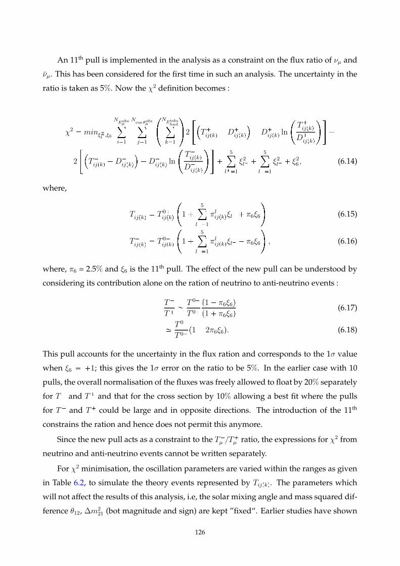
An 11th pull is implemented in the analysis as a constraint on the flux ratio of νµ and

νµ. This has been considered for the first time in such an analysis. The uncertainty in the

ratio is taken as 5%. Now the χ2 definition becomes :

χ2 minξ

l,ξ6

NEobsµ¸

i1

Ncos θobsµ¸

j1

NE1obshad¸

k1

2

T

ijpkqD

ijpkq

D

ijpkqln

T

ijpkq

D

ijpkq

2

T

ijpkqD

ijpkq

D

ijpkqln

T

ijpkq

D

ijpkq

5¸

l1

ξ2l

5¸

l1

ξ2l ξ26, (6.14)

where,

T

ijpkq T 0

ijpkq

1

5

l1

πl

ijpkqξl π6ξ6

(6.15)

T

ijpkq T 0

ijpkq

1

5¸

l1

πl

ijpkqξl π6ξ6

, (6.16)

where, π6 = 2.5% and ξ6 is the 11th pull. The effect of the new pull can be understood by

considering its contribution alone on the ration of neutrino to anti-neutrino events :

T

T

T 0

T 0

p1 π6ξ6q

p1 π6ξ6q(6.17)

T 0

T 0p1 2π6ξ6q. (6.18)

This pull accounts for the uncertainty in the flux ration and corresponds to the 1σ value

when ξ6 1; this gives the 1σ error on the ratio to be 5%. In the earlier case with 10

pulls, the overall normalisation of the fluxes was freely allowed to float by 20% separately

for T and T and that for the cross section by 10% allowing a best fit where the pulls

for T and T could be large and in opposite directions. The introduction of the 11th

constrains the ration and hence does not permit this anymore.

Since the new pull acts as a constraint to the T

µ T

µ ratio, the expressions for χ2 from

neutrino and anti-neutrino events cannot be written separately.

For χ2 minimisation, the oscillation parameters are varied within the ranges as given

in Table 6.2, to simulate the theory events represented by Tijpkq. The parameters which

will not affect the results of this analysis, i.e, the solar mixing angle and mass squared dif-

ference θ12, ∆m221 (bot magnitude and sign) are kept ”fixed“. Earlier studies have shown

126

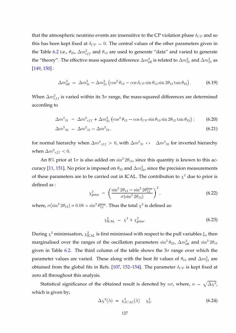
that the atmospheric neutrino events are insensitive to the CP violation phase δCP and so

this has been kept fixed at δCP 0. The central values of the other parameters given in

the Table 6.2 i.e., θ23, ∆m2

eff and θ13 are used to generate “data” and varied to generate

the “theory”. The effective mass squared difference ∆m2

eff is related to ∆m231 and∆m2

21 as

[149, 150] :

∆m2

eff ∆m2

31 ∆m2

21

cos2 θ12 cos δCP sin θ13 sin 2θ12 tan θ23

. (6.19)

When ∆m2

eff is varied within its 3σ range, the mass-squared differences are determined

according to

∆m231 ∆m2

eff ∆m2

21

cos2 θ12 cos δCP sin θ13 sin 2θ12 tan θ23

; (6.20)

∆m232 ∆m2

31 ∆m221, (6.21)

for normal hierarchy when ∆m2eff ¡ 0, with ∆m2

31 Ø ∆m232 for inverted hierarchy

when ∆m2eff 0.

An 8% prior at 1σ is also added on sin2 2θ13, since this quantity is known to this ac-

curacy [11, 151]. No prior is imposed on θ23 and∆m232, since the precision measurements

of these parameters are to be carried out in ICAL. The contribution to χ2 due to prior is

defined as :

χ2

prior

sin2 2θ13 sin2 2θtrue13

σpsin2 2θ13q

2

, (6.22)

where, σpsin2 2θ13q = 0.08 sin2 θtrue13 . Thus the total χ2 is defined as:

χ2

ICAL χ2 χ2

prior. (6.23)

During χ2 minimisation, χ2

ICAL is first minimised with respect to the pull variables ξl, then

marginalised over the ranges of the oscillation parameters sin2 θ23, ∆m2

eff and sin2 2θ13

given in Table 6.2. The third column of the table shows the 3σ range over which the

parameter values are varied. These along with the best fit values of θ12 and ∆m221 are

obtained from the global fits in Refs. [107, 152–154]. The parameter δCP is kept fixed at

zero all throughout this analysis.

Statistical significance of the obtained result is denoted by nσ, where, n

a

∆χ2,

which is given by;

∆χ2pλq χ2

ICALpλq χ2

0, (6.24)

127

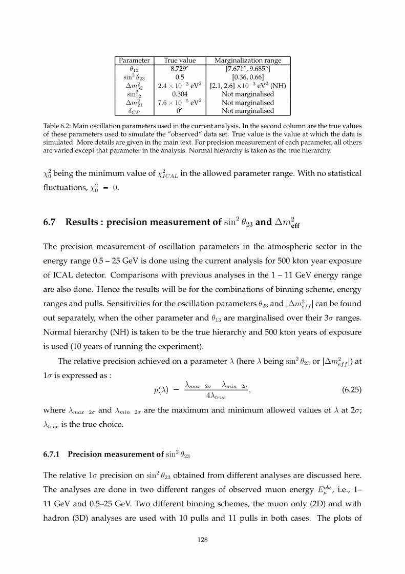
Parameter True value Marginalization rangeθ13 8.729 [7.671, 9.685]

sin2 θ23 0.5 [0.36, 0.66]

∆m232 2.4 103 eV2 [2.1, 2.6]103 eV2 (NH)

sin212 0.304 Not marginalised

∆m221 7.6 105 eV2 Not marginalised

δCP 0 Not marginalised

Table 6.2: Main oscillation parameters used in the current analysis. In the second column are the true valuesof these parameters used to simulate the ”observed“ data set. True value is the value at which the data issimulated. More details are given in the main text. For precision measurement of each parameter, all othersare varied except that parameter in the analysis. Normal hierarchy is taken as the true hierarchy.

χ20being the minimum value of χ2

ICAL in the allowed parameter range. With no statistical

fluctuations, χ20 0.

6.7 Results : precision measurement of sin2 θ23 and ∆m2eff

The precision measurement of oscillation parameters in the atmospheric sector in the

energy range 0.5 – 25 GeV is done using the current analysis for 500 kton year exposure

of ICAL detector. Comparisons with previous analyses in the 1 – 11 GeV energy range

are also done. Hence the results will be for the combinations of binning scheme, energy

ranges and pulls. Sensitivities for the oscillation parameters θ23 and |∆m2

eff | can be found

out separately, when the other parameter and θ13 are marginalised over their 3σ ranges.

Normal hierarchy (NH) is taken to be the true hierarchy and 500 kton years of exposure

is used (10 years of running the experiment).

The relative precision achieved on a parameter λ (here λ being sin2 θ23 or |∆m2

eff |) at

1σ is expressed as :

ppλq λmax2σ λmin2σ

4λtrue, (6.25)

where λmax2σ and λmin2σ are the maximum and minimum allowed values of λ at 2σ;

λtrue is the true choice.

6.7.1 Precision measurement of sin2 θ23

The relative 1σ precision on sin2 θ23 obtained from different analyses are discussed here.

The analyses are done in two different ranges of observed muon energy Eobsµ , i.e., 1–

11 GeV and 0.5–25 GeV. Two different binning schemes, the muon only (2D) and with

hadron (3D) analyses are used with 10 pulls and 11 pulls in both cases. The plots of

128

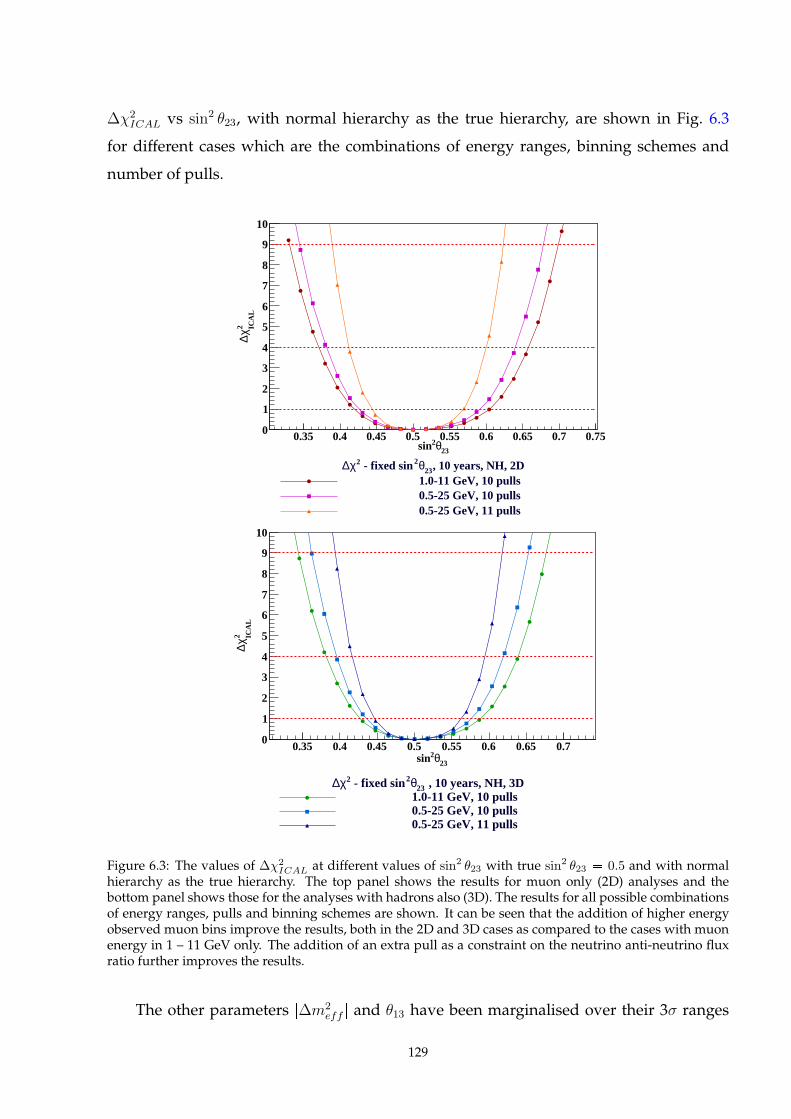
∆χ2

ICAL vs sin2 θ23, with normal hierarchy as the true hierarchy, are shown in Fig. 6.3

for different cases which are the combinations of energy ranges, binning schemes and

number of pulls.

23θ2sin0.35 0.4 0.45 0.5 0.55 0.6 0.65 0.7 0.75

ICA

L

2 χ∆

0

1

2

3

4

5

6

7

8

9

10

, 10 years, NH, 2D23θ2 - fixed sin2χ∆1.0-11 GeV, 10 pulls0.5-25 GeV, 10 pulls0.5-25 GeV, 11 pulls

23θ2sin0.35 0.4 0.45 0.5 0.55 0.6 0.65 0.7

ICA

L

2 χ∆

0

1

2

3

4

5

6

7

8

9

10

, 10 years, NH, 3D23θ2 - fixed sin2χ∆1.0-11 GeV, 10 pulls0.5-25 GeV, 10 pulls0.5-25 GeV, 11 pulls

Figure 6.3: The values of ∆χ2ICAL at different values of sin2 θ23 with true sin2 θ23 0.5 and with normal

hierarchy as the true hierarchy. The top panel shows the results for muon only (2D) analyses and thebottom panel shows those for the analyses with hadrons also (3D). The results for all possible combinationsof energy ranges, pulls and binning schemes are shown. It can be seen that the addition of higher energyobserved muon bins improve the results, both in the 2D and 3D cases as compared to the cases with muonenergy in 1 – 11 GeV only. The addition of an extra pull as a constraint on the neutrino anti-neutrino fluxratio further improves the results.

The other parameters |∆m2

eff | and θ13 have been marginalised over their 3σ ranges

129

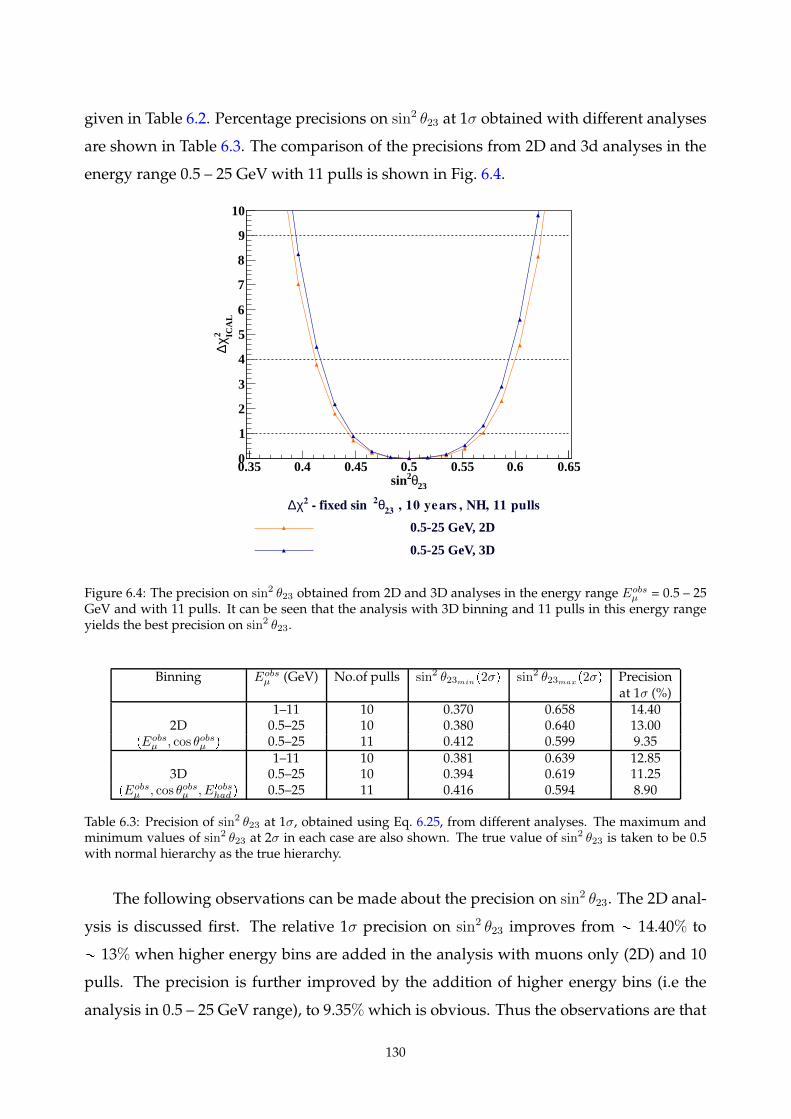
given in Table 6.2. Percentage precisions on sin2 θ23 at 1σ obtained with different analyses

are shown in Table 6.3. The comparison of the precisions from 2D and 3d analyses in the

energy range 0.5 – 25 GeV with 11 pulls is shown in Fig. 6.4.

23θ2sin0.35 0.4 0.45 0.5 0.55 0.6 0.65

ICA

L2 χ

∆

0

1

2

3

4

5

6

7

8

9

10

, 10 years , NH, 11 pulls23

θ2 fixed sin2χ∆

0.5-25 GeV, 2D

0.5-25 GeV, 3D

Figure 6.4: The precision on sin2 θ23 obtained from 2D and 3D analyses in the energy range Eobsµ = 0.5 – 25

GeV and with 11 pulls. It can be seen that the analysis with 3D binning and 11 pulls in this energy rangeyields the best precision on sin2 θ23.

Binning Eobsµ (GeV) No.of pulls sin2 θ23min

p2σq sin2 θ23maxp2σq Precision

at 1σ (%)1–11 10 0.370 0.658 14.40

2D 0.5–25 10 0.380 0.640 13.00pEobs

µ , cos θobsµ q 0.5–25 11 0.412 0.599 9.35

1–11 10 0.381 0.639 12.853D 0.5–25 10 0.394 0.619 11.25


had q 0.5–25 11 0.416 0.594 8.90

Table 6.3: Precision of sin2 θ23 at 1σ, obtained using Eq. 6.25, from different analyses. The maximum andminimum values of sin2 θ23 at 2σ in each case are also shown. The true value of sin2 θ23 is taken to be 0.5with normal hierarchy as the true hierarchy.

The following observations can be made about the precision on sin2 θ23. The 2D anal-

ysis is discussed first. The relative 1σ precision on sin2 θ23 improves from 14.40% to

13% when higher energy bins are added in the analysis with muons only (2D) and 10

pulls. The precision is further improved by the addition of higher energy bins (i.e the

analysis in 0.5 – 25 GeV range), to 9.35%which is obvious. Thus the observations are that

130

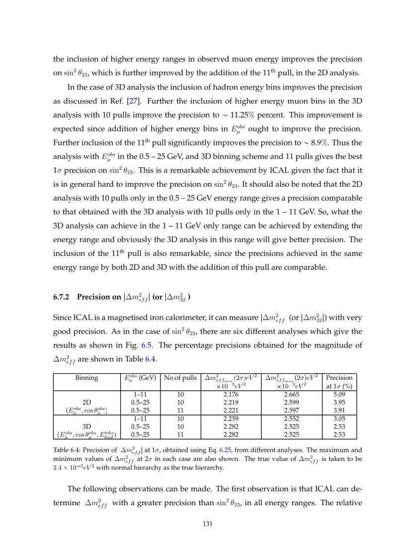
the inclusion of higher energy ranges in observed muon energy improves the precision

on sin2 θ23, which is further improved by the addition of the 11th pull, in the 2D analysis.

In the case of 3D analysis the inclusion of hadron energy bins improves the precision

as discussed in Ref. [27]. Further the inclusion of higher energy muon bins in the 3D

analysis with 10 pulls improve the precision to 11.25% percent. This improvement is

expected since addition of higher energy bins in Eobsµ ought to improve the precision.

Further inclusion of the 11th pull significantly improves the precision to 8.9%. Thus the

analysis with Eobsµ in the 0.5 – 25 GeV, and 3D binning scheme and 11 pulls gives the best

1σ precision on sin2 θ23. This is a remarkable achievement by ICAL given the fact that it

is in general hard to improve the precision on sin2 θ23. It should also be noted that the 2D

analysis with 10 pulls only in the 0.5 – 25 GeV energy range gives a precision comparable

to that obtained with the 3D analysis with 10 pulls only in the 1 – 11 GeV. So, what the

3D analysis can achieve in the 1 – 11 GeV only range can be achieved by extending the

energy range and obviously the 3D analysis in this range will give better precision. The

inclusion of the 11th pull is also remarkable, since the precisions achieved in the same

energy range by both 2D and 3D with the addition of this pull are comparable.

6.7.2 Precision on |∆m2

eff | (or |∆m232|)

Since ICAL is a magnetised iron calorimeter, it can measure |∆m2

eff | (or |∆m232|) with very

good precision. As in the case of sin2 θ23, there are six different analyses which give the

results as shown in Fig. 6.5. The percentage precisions obtained for the magnitude of

∆m2

eff are shown in Table 6.4.

Binning Eobsµ (GeV) No.of pulls ∆m2

effminp2σqeV 2 ∆m2

effmaxp2σqeV 2 Precision

103eV 2103eV 2 at 1σ (%)

1–11 10 2.176 2.665 5.092D 0.5–25 10 2.219 2.599 3.95

pEobsµ , cos θobsµ q 0.5–25 11 2.221 2.597 3.91

1–11 10 2.259 2.552 3.053D 0.5–25 10 2.282 2.525 2.53


had q 0.5–25 11 2.282 2.525 2.53

Table 6.4: Precision of |∆m2

eff | at 1σ, obtained using Eq. 6.25, from different analyses. The maximum and

minimum values of ∆m2

eff at 2σ in each case are also shown. The true value of ∆m2

eff is taken to be

2.4 103eV 2 with normal hierarchy as the true hierarchy.

The following observations can be made. The first observation is that ICAL can de-

termine |∆m2

eff | with a greater precision than sin2 θ23, in all energy ranges. The relative

131

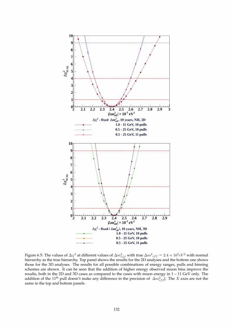
2 eV-3 10×| eff2m∆|

2 2.1 2.2 2.3 2.4 2.5 2.6 2.7 2.8 2.9 3

ICA

L2 χ

∆

0

1

2

3

4

5

6

7

8

9

10

, 10 years, NH, 2D2eff

m∆ fixed 2χ∆1.0 - 11 GeV, 10 pulls0.5 - 25 GeV, 10 pulls0.5 - 25 GeV, 11 pulls

2 eV-3 10×| eff2m∆|

2 2.1 2.2 2.3 2.4 2.5 2.6 2.7 2.8 2.9

ICA

L2 χ

∆

0

1

2

3

4

5

6

7

8

9

10

|, 10 years, NH, 3D2eff

m∆ fixed |2χ∆1.0 - 11 GeV, 10 pulls0.5 - 25 GeV, 10 pulls0.5 - 25 GeV, 11 pulls

Figure 6.5: The values of ∆χ2 at different values of ∆m2eff with true ∆m2

eff 2.4 103eV 2 with normalhierarchy as the true hierarchy. Top panel shows the results for the 2D analyses and the bottom one showsthose for the 3D analyses. The results for all possible combinations of energy ranges, pulls and binningschemes are shown. It can be seen that the addition of higher energy observed muon bins improve theresults, both in the 2D and 3D cases as compared to the cases with muon energy in 1 – 11 GeV only. Theaddition of the 11th pull doesn’t make any difference in the precision of |∆m2

eff |. The X axes are not thesame in the top and bottom panels.

132

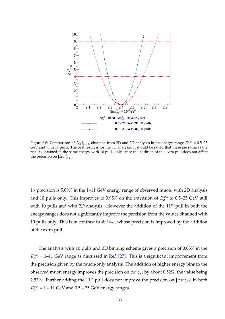
2 eV-3 10×| eff2m∆|

2 2.1 2.2 2.3 2.4 2.5 2.6 2.7 2.8

ICA

L2 χ

∆

0

1

2

3

4

5

6

7

8

9

10

, 10 years, NH2eff

m∆ fixed 2χ∆0.5 - 25 GeV, 2D; 11 pulls

0.5 - 25 GeV, 3D; 11 pulls

Figure 6.6: Comparison of ∆χ2ICAL obtained from 2D and 3D analyses in the energy range Eobs

µ = 0.5–25GeV and with 11 pulls. The best result is for the 3D analysis. It should be noted that these are same as theresults obtained in the same energy with 10 pulls only, since the addition of the extra pull does not affectthe precision on |∆m2

eff |.

1σ precision is 5.09% in the 1–11 GeV energy range of observed muon, with 2D analysis

and 10 pulls only. This improves to 3.95% on the extension of Eobsµ to 0.5–25 GeV, still

with 10 pulls and with 2D analysis. However the addition of the 11th pull in both the

energy ranges does not significantly improve the precision from the values obtained with

10 pulls only. This is in contrast to sin2 θ23, whose precision is improved by the addition

of the extra pull.

The analysis with 10 pulls and 3D binning scheme gives a precision of 3.05% in the

Eobsµ = 1–11 GeV range as discussed in Ref. [27]. This is a significant improvement from

the precision given by the muon-only analysis. The addition of higher energy bins in the

observed muon energy improves the precision on∆m2

eff by about 0.52%, the value being

2.53%. Further adding the 11th pull does not improve the precision on |∆m2

eff | in both

Eobsµ = 1 – 11 GeV and 0.5 – 25 GeV energy ranges.

133

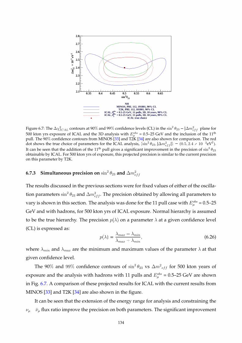
23θ2sin0.35 0.4 0.45 0.5 0.55 0.6 0.65

2 e

V-3

10

× 322

m∆

2.1

2.2

2.3

2.4

2.5

2.6

2.7

2.8

NHMINOS, PRL 112, 191801, 90% CL

T2K, PRL 112, 181801, 90% CL = 0.5-25 GeV, 11 pulls, 3D, 10 years, 90% CLµ

obsICAL, E = 0.5-25 GeV, 11 pulls, 3D, 10 years, 99% CLµ

obsICAL, EICAL true choice

Figure 6.7: The∆χ2ICAL contours at 90% and 99% confidence levels (CL) in the sin2 θ23 |∆m2

eff | plane for

500 kton yrs exposure of ICAL and the 3D analysis with Eobsµ = 0.5–25 GeV and the inclusion of the 11th

pull. The 90% confidence contours from MINOS [33] and T2K [34] are also shown for comparison. The reddot shows the true choice of parameters for the ICAL analysis, psin2 θ23, |∆m2

eff |q p0.5, 2.4 103eV2q.

It can be seen that the addition of the 11th pull gives a significant improvement in the precision of sin2 θ23obtainable by ICAL. For 500 kton yrs of exposure, this projected precision is similar to the current precisionon this parameter by T2K.

6.7.3 Simultaneous precision on sin2 θ23 and ∆m2

eff

The results discussed in the previous sections were for fixed values of either of the oscilla-

tion parameters sin2 θ23 and ∆m2

eff . The precision obtained by allowing all parameters to

vary is shown in this section. The analysis was done for the 11 pull case withEobsµ = 0.5–25

GeV and with hadrons, for 500 kton yrs of ICAL exposure. Normal hierarchy is assumed

to be the true hierarchy. The precision ppλq on a parameter λ at a given confidence level

(CL) is expressed as:

ppλq λmax λmin

λmax λmin, (6.26)

where λmin and λmax are the minimum and maximum values of the parameter λ at that

given confidence level.

The 90% and 99% confidence contours of sin2 θ23 vs ∆m2eff for 500 kton years of

exposure and the analysis with hadrons with 11 pulls and Eobsµ = 0.5–25 GeV are shown

in Fig. 6.7. A comparison of these projected results for ICAL with the current results from

MINOS [33] and T2K [34] are also shown in the figure.

It can be seen that the extension of the energy range for analysis and constraining the

νµ νµ flux ratio improve the precision on both parameters. The significant improvement

134

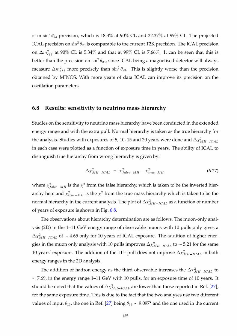
is in sin2 θ23 precision, which is 18.3% at 90% CL and 22.37% at 99% CL. The projected

ICAL precision on sin2 θ23 is comparable to the current T2K precision. The ICAL precision

on ∆m2

eff at 90% CL is 5.34% and that at 99% CL is 7.66%. It can be seen that this is

better than the precision on sin2 θ23, since ICAL being a magnetised detector will always

measure ∆m2

eff more precisely than sin2 θ23. This is slightly worse than the precision

obtained by MINOS. With more years of data ICAL can improve its precision on the

oscillation parameters.

6.8 Results: sensitivity to neutrino mass hierarchy

Studies on the sensitivity to neutrinomass hierarchy have been conducted in the extended

energy range and with the extra pull. Normal hierarchy is taken as the true hierarchy for

the analysis. Studies with exposures of 5, 10, 15 and 20 years were done and ∆χ2

MHICAL

in each case were plotted as a function of exposure time in years. The ability of ICAL to

distinguish true hierarchy from wrong hierarchy is given by:

∆χ2

MHICAL χ2

falseMH χ2

trueMH , (6.27)

where χ2

falseMH is the χ2 from the false hierarchy, which is taken to be the inverted hier-

archy here and χ2trueMH is the χ2 from the true mass hierarchy which is taken to be the

normal hierarchy in the current analysis. The plot of∆χ2

MHICAL as a function of number

of years of exposure is shown in Fig. 6.8.

The observations about hierarchy determination are as follows. The muon-only anal-

ysis (2D) in the 1–11 GeV energy range of observable muons with 10 pulls only gives a

∆χ2

MHICAL of 4.65 only for 10 years of ICAL exposure. The addition of higher ener-

gies in the muon only analysis with 10 pulls improves ∆χ2MHICAL to 5.21 for the same

10 years’ exposure. The addition of the 11th pull does not improve ∆χ2MHICAL in both

energy ranges in the 2D analysis.

The addition of hadron energy as the third observable increases the ∆χ2

MHICAL to

7.69, in the energy range 1–11 GeV with 10 pulls, for an exposure time of 10 years. It

should be noted that the values of ∆χ2MHICAL are lower than those reported in Ref. [27],

for the same exposure time. This is due to the fact that the two analyses use two different

values of input θ13, the one in Ref. [27] being θ13 9.097 and the one used in the current

135

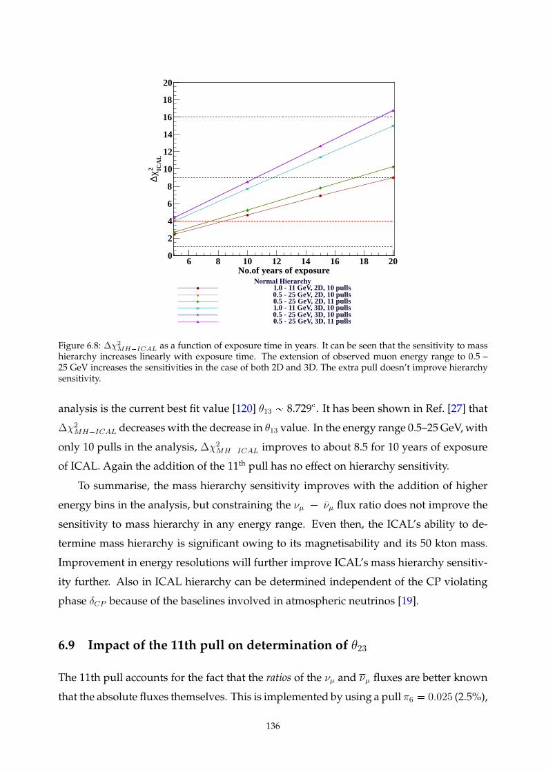
No.of years of exposure6 8 10 12 14 16 18 20

ICA

L2 χ

∆

0

2

4

6

8

10

12

14

16

18

20

Normal Hierarchy1.0 - 11 GeV, 2D, 10 pulls0.5 - 25 GeV, 2D, 10 pulls0.5 - 25 GeV, 2D, 11 pulls1.0 - 11 GeV, 3D, 10 pulls0.5 - 25 GeV, 3D, 10 pulls0.5 - 25 GeV, 3D, 11 pulls

Figure 6.8: ∆χ2MHICAL as a function of exposure time in years. It can be seen that the sensitivity to mass

hierarchy increases linearly with exposure time. The extension of observed muon energy range to 0.5 –25 GeV increases the sensitivities in the case of both 2D and 3D. The extra pull doesn’t improve hierarchysensitivity.

analysis is the current best fit value [120] θ13 8.729. It has been shown in Ref. [27] that

∆χ2MHICAL decreases with the decrease in θ13 value. In the energy range 0.5–25 GeV,with

only 10 pulls in the analysis, ∆χ2MHICAL improves to about 8.5 for 10 years of exposure

of ICAL. Again the addition of the 11th pull has no effect on hierarchy sensitivity.

To summarise, the mass hierarchy sensitivity improves with the addition of higher

energy bins in the analysis, but constraining the νµ νµ flux ratio does not improve the

sensitivity to mass hierarchy in any energy range. Even then, the ICAL’s ability to de-

termine mass hierarchy is significant owing to its magnetisability and its 50 kton mass.

Improvement in energy resolutions will further improve ICAL’s mass hierarchy sensitiv-

ity further. Also in ICAL hierarchy can be determined independent of the CP violating

phase δCP because of the baselines involved in atmospheric neutrinos [19].

6.9 Impact of the 11th pull on determination of θ23

The 11th pull accounts for the fact that the ratios of the νµ and νµ fluxes are better known

that the absolute fluxes themselves. This is implemented by using a pull π6 0.025 (2.5%),

136

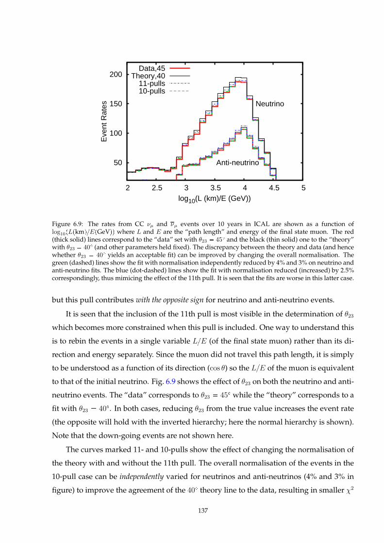
50

100

150

200

2 2.5 3 3.5 4 4.5 5

Eve

nt R

ates

log10(L (km)/E (GeV))

Neutrino

Anti-neutrino

Data,45

11-pullsTheory,40

10-pulls

Figure 6.9: The rates from CC νµ and νµ events over 10 years in ICAL are shown as a function oflog10pLpkmqEpGeVqq where L and E are the “path length” and energy of the final state muon. The red(thick solid) lines correspond to the “data” set with θ23 45 and the black (thin solid) one to the “theory”with θ23 40 (and other parameters held fixed). The discrepancy between the theory and data (and hencewhether θ23 40 yields an acceptable fit) can be improved by changing the overall normalisation. Thegreen (dashed) lines show the fit with normalisation independently reduced by 4% and 3% on neutrino andanti-neutrino fits. The blue (dot-dashed) lines show the fit with normalisation reduced (increased) by 2.5%correspondingly, thus mimicing the effect of the 11th pull. It is seen that the fits are worse in this latter case.

but this pull contributes with the opposite sign for neutrino and anti-neutrino events.

It is seen that the inclusion of the 11th pull is most visible in the determination of θ23

which becomes more constrained when this pull is included. One way to understand this

is to rebin the events in a single variable LE (of the final state muon) rather than its di-

rection and energy separately. Since the muon did not travel this path length, it is simply

to be understood as a function of its direction (cos θ) so the LE of the muon is equivalent

to that of the initial neutrino. Fig. 6.9 shows the effect of θ23 on both the neutrino and anti-

neutrino events. The “data” corresponds to θ23 45 while the “theory” corresponds to a

fit with θ23 40. In both cases, reducing θ23 from the true value increases the event rate

(the opposite will hold with the inverted hierarchy; here the normal hierarchy is shown).

Note that the down-going events are not shown here.

The curves marked 11- and 10-pulls show the effect of changing the normalisation of

the theory with and without the 11th pull. The overall normalisation of the events in the

10-pull case can be independently varied for neutrinos and anti-neutrinos (4% and 3% in

figure) to improve the agreement of the 40 theory line to the data, resulting in smaller χ2

137

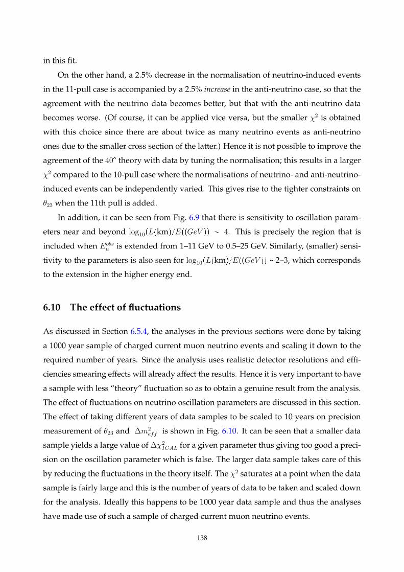
in this fit.

On the other hand, a 2.5% decrease in the normalisation of neutrino-induced events

in the 11-pull case is accompanied by a 2.5% increase in the anti-neutrino case, so that the

agreement with the neutrino data becomes better, but that with the anti-neutrino data

becomes worse. (Of course, it can be applied vice versa, but the smaller χ2 is obtained

with this choice since there are about twice as many neutrino events as anti-neutrino

ones due to the smaller cross section of the latter.) Hence it is not possible to improve the

agreement of the 40 theory with data by tuning the normalisation; this results in a larger

χ2 compared to the 10-pull case where the normalisations of neutrino- and anti-neutrino-

induced events can be independently varied. This gives rise to the tighter constraints on

θ23 when the 11th pull is added.

In addition, it can be seen from Fig. 6.9 that there is sensitivity to oscillation param-

eters near and beyond log10pLpkmqEp(GeV qq 4. This is precisely the region that is

included when Eobsµ is extended from 1–11 GeV to 0.5–25 GeV. Similarly, (smaller) sensi-

tivity to the parameters is also seen for log10pLpkmqEp(GeV qq 2–3, which corresponds

to the extension in the higher energy end.

6.10 The effect of fluctuations

As discussed in Section 6.5.4, the analyses in the previous sections were done by taking

a 1000 year sample of charged current muon neutrino events and scaling it down to the

required number of years. Since the analysis uses realistic detector resolutions and effi-

ciencies smearing effects will already affect the results. Hence it is very important to have

a sample with less “theory” fluctuation so as to obtain a genuine result from the analysis.

The effect of fluctuations on neutrino oscillation parameters are discussed in this section.

The effect of taking different years of data samples to be scaled to 10 years on precision

measurement of θ23 and |∆m2

eff | is shown in Fig. 6.10. It can be seen that a smaller data

sample yields a large value of∆χ2ICAL for a given parameter thus giving too good a preci-

sion on the oscillation parameter which is false. The larger data sample takes care of this

by reducing the fluctuations in the theory itself. The χ2 saturates at a point when the data

sample is fairly large and this is the number of years of data to be taken and scaled down

for the analysis. Ideally this happens to be 1000 year data sample and thus the analyses

have made use of such a sample of charged current muon neutrino events.

138

No.of years of data to be sampled 100 200 300 400 500 600 700 800 900 1000

ICA

L2 χ∆

0

1

2

3

4

5

6

7

8

9

10

vs Actual data sample which is scaled2χ∆

° = 3923θ0.5 - 25 GeV, 3D, 10 pulls,

No.of years of years of data to be sampled100 200 300 400 500 600 700 800 900 1000

ICA

L2 χ

∆

0

1

2

3

4

5

6

7

8

9

10

vs Actual data sample which is scaled2χ∆

2 eV-3 10×| = 2.50 eff2m∆0.5 - 25 GeV, 3D, 10 pulls, |

Figure 6.10: The value of∆χ2ICAL vs the number of years of data to be scaled to 10 years for θ23 39 (left)

and |∆m2eff | 2.5 103ev2 (right). It can be seen that the scaling of only 100 years of data gives too

high a χ2 which is even more prominent in the case of ∆m2eff . As the number of years of data sample to

be scaled increases, the value of χ2 also comes down as well as saturates for large enough data samples.

6.11 Chapter Summary

The proposedmagnetised Iron Calorimeter detector (ICAL) at INO aims to probe the neu-

trino oscillation parameters by observing atmospheric neutrino oscillations and studying

their Earth matter effects as they propagate through the Earth. This will be done by de-

tecting (mainly) the charged current interactions of νµ and νµ in the detector by means of

the final state muons. The detector, which is optimised for the detection of muons in the

GeV energy range will have a magnetic field which will enable the distinction of νµ and

νµ events by identifying the charge of the muon in the final state, thus making ICAL an

excellent detector to determine neutrino mass hierarchy. Not only this, the magnetic field

helps to improve the precision measurement of themixing angle θ23 and |∆m2

eff | (|∆m232|).

Muons are not the only final state particles in the charged current interactions. Hadrons

which produce a shower unlike the clean tracks of muons, are also present. Thus to study

the sensitivities of the ICAL to neutrino oscillation parameters two different types of anal-

yses can be used, one with muon energy and direction only as the observables used to bin

events (2D binning scheme); and the other in which hadron energy, along with muon en-

ergy and direction (3D binning scheme) is used as an observable to bin the events. It has

been shown elsewhere that the use of hadron energy improves the sensitivities of ICAL

significantly [27]. But these studies have been conducted in the restricted energy range

of 1 – 11 GeV and with 10 systematic pulls only. It should be noted that instead of re-

139

constructing the neutrino energy and direction and then binning in neutrino energy the

analyses have been done by taking all the observables separately. This is because of the

poor energy and direction resolution of neutrinos in ICAL detector owing to the fact that

they are driven by the responses of ICAL detector to hadrons, which are worse compared

to those of muons. Still the addition of the extra information regarding hadrons improves

the sensitivity of ICAL to oscillation parameters.

Knowing that hadron energy information can improve the sensitivities it is interest-

ing to probe new possibilities of improving the detector’s sensitivities since any improve-

ment in the sensitivities is going to impact the global values of these parameters and it is

important that we extract as much information as possible from different analyses. Thus

the study of the effect of extending the observed muon energy Eobsµ range to 0.5 – 25 GeV

along with the addition of a pull in the form of a constraint on the ratio of atmospheric νµ

- νµ fluxes becomes significant. Both 2D and 3D binning scheme are used for the analyses

and the results for Eobsµ = 1 – 11 GeV and 0.5 – 25 GeV are compared with one another.

The 2D binning scheme with pEobsµ , cos θobsµ q , where cos θobsµ represents the observed muon

direction, has 15 non-uniform bins in Eobsµ and 21 uniform bins in cos θobsµ . In the 3D bin-

ning scheme with pEobsµ , cos θobsµ , Eobs

hadq, the same muon bins along with 4 bins in observed

hadron energy are used.

The relative 1σ precision on sin2 θ23 and |∆m2

eff | (|∆m232|) improves with the exten-

sion of energy range, the major effect coming from the addition of higher energy bins

beyond 11 GeV. Though the precision on |∆m2

eff | (|∆m232|) is very good, it is the precision

on sin2 θ23 which improves significantly, which is also the main highlight of this analy-

sis. The effect on precisions attainable with 500 kton year exposure (10 years of run) are

mentioned here. In the 2D case with 10 pulls only, the 1σ precision on sin2 θ23 which was

14.40% in the 1 – 11 GeV range, improves to 13.00% on extending the energy range

to 0.5 – 25 GeV. Similarly in the 3D case with 10 pulls only, the same precision improves

from 12.85% to 11.25% on increasing the energy range. The addition of the extra pull

improves the precision further in all energy ranges. The best best precision on sin2 θ23

achievable with 500 kton years of ICAL 8.90% with the 3D binning scheme, in the 0.5 –

25 GeV energy and with 11 systematic pulls. This is a significant improvement over all

the previous analyses of ICAL physics and will contribute to the global fits of neutrino

oscillation parameters.

The relative precision of |∆m2

eff | (|∆m232|) in the 1 – 11 GeV range with 10 pulls only, is

140

5.09%with 2D binning scheme. The extension of energy range to 0.5 – 25 GeV improves

this precision to 3.95%. The 3D binning scheme with 10 pulls only yields a precision

of 3.05% in the 1 – 11 GeV energy range, the precision slightly improves to 2.53% in

the 0.5 – 25 GeV. Addition of the 11th pulls does not improve the precisions on |∆m2

eff |

(|∆m232|) from their values obtained with 10 pulls only. Thus unlike sin2 θ23, the constraint

on the flux ratio of νµ and νµ has no effect on |∆m2

eff | (|∆m232|).

The neutrino mass hierarchy sensitivity of ICAL was also shown to improve signifi-

cantly with the 3D binning scheme in the energy range 1 – 11 GeV [27]. The extension of

Eobsµ to 0.5 – 25 GeVs improves the hierarchy sensitivity in both 2D and 3D analyses with

10 pulls. The best value of ∆χ2

ICAL achievable with 500 kton years of exposure is 8.523

obtained from 3D analysis in the 0.5 – 25 GeV range of observed muon energy. Addition

of the 11th pulls does not affect mass hierarchy determination.

The studies presented here assume that there is perfection separation between differ-

ent types of events. The event identification efficiency will also affect the results of the

analysis since they will determine the number of events in each bin. Also the resolutions

for hadrons and muons used in this analysis were obtained from simulations of the INO

ICAL detector using GEANT-4. Improvements in the reconstruction efficiencies and res-

olutions will definitely give better results. It is also worthwhile thinking about alterations

in detector geometry if needed and plausible to make the detector more efficient and one

with better resolutions. Also the current studies are all done with the atmospheric neu-

trino flux at the Super Kamiokande site. The fluxes at Theni where ICAL will be built

have to be used for next level of analysis. Also the effect of adding hadron direction as a

fourth observable in the analysis still have to be studied, it remains to be checked if this

information will give better or worse results than the existing ones. The physics results of

ICAL have the capability to impact global fits to neutrino data and thus any new analysis

will open a window to understanding the neutrino oscillation parameters better on the

whole.

141

Part IV

Summary and future scope

7 Summary and Future Scope

Many neutrino oscillation experiments all over the world are probing neutrinos from

various sources, over different regions of LE to get more insight into the intrinsic prop-

erties of neutrinos such as their masses, mixing angles and mass ordering and also to

probe CP violation through the leptonic sector via studying neutrinos. The proposed

Iron-CALorimater (ICAL) experiment at the upcoming India-based Neutrino Observa-

tory (INO) is a large scale Neutrino Physics experiment which aims to determine neutrino

mass hierarchy and perform precision measurements of neutrino oscillation parameters

|∆m232| and θ23, by observing atmospheric neutrinos coming from the other side of the

Earth. The 50 kilo ton magnetisable, detector, to be situated under the 1595 m peak of

Bodi West Hills in Theni District of Tamil Nadu has tremendous physics potential. The

simulation studies on the physics of hadrons in the ICAL detector and the physics reach

of ICAL to neutrino oscillations have been discussed in this thesis. A summary of these

discussions is given in the first part of this chapter. Since ICAL is such a huge detector, it

is interesting to explore what other physics it can do other than neutrino oscillations. The

future scopes are discussed in the second part of this thesis.

7.1 Summary

As mentioned above, the ICAL detector at INO will be a 50 kton magnetisable detector

which will detect atmospheric neutrinos and probe Earth matter effects on their propa-

gation to determine neutrino mass hierarchy and conduct precision measurements of the

mixing angle θ23 and |∆m232|. Due to its magnetisability, ICAL can distinguish between

µ and µ produced in the final state of the charged current interactions of νµ and νµ with

the iron in the detector. This imparts to ICAL the capability to determine neutrino mass

hierarchy.

Not only muons but hadrons are also produced in the final state of these charged

current interactions. Even though the ICAL detector is optimised for muon detection

and has excellent muon momentum and direction resolutions, it is necessary to extract

as much information from the hadrons as possible. Simulation studies of single pions

propagated through the ICAL detector simulated using a GEANT-4 based simulation

frames work was done. From the studies it was seen that the energy resolution of fixed

energy single pions is 0.86?

E at 1 GeV and 0.36?

E at 15 GeV for the default iron plate

thickness of 5.6 cm.

Studies on the dependence of hadron energy resolution on iron plate thickness were

done. The studies showed that the dependence is not a naive square root dependence

as seen in the case of hadrons of very high energies. The dependence of the stochastic

coefficient a from the relation pσEq2 a2E b2, was studied and it was found to have

the following properties. For the direction averaged case, in the low energy range of 2–

4.75 GeV, the value of a increases from a 0.651 for 1.5 cm thick iron to a 0.969 for 8

cm iron. In the higher energy range 5–15 GeV, the value of a varies between 0.702 and

0.974. In the full energy range 2–15 GeV, the variation is between a 0.709 to a 0.985.

The parametrisation of the thickness dependence of this stochastic coefficient a using the

relation aptq p0tp1 p2 shows that the dependence is not a

?

t (where t is the iron plate

thickness) as in the case of very high energies. Rather it is energy dependent and the

thickness dependent term has an exponent p1 which is 1.13 in the 2–4.75 GeV energy

range and 0.73 in the 5–15 GeV energy range. The smallness of the coefficient p0 makes

the contribution of this term less significant than that of the constant term p2 which is

always around 0.6. The term p2 attributes to the residual resolution which is due to the

intrinsic uncertainties of strong interactions, fluctuations and detector geometry, indicat-

ing that there will always be a finite uncertainty the estimation of hadron energy even if

the plate thickness is reduced to infinitesimally small values. An alternate parametrisa-

tion of the plate thickness dependence of σ?

E as, σ?

E q0tq1 q2 also showed that

the effect of the presence of the residual resolution on hadron energy response.

The direction dependence of the thickness dependence was also studied. For a given

thickness it was found that the energy response is the worst for the most horizontal di-

rections as expected, improves with the increase in cos θ values, but the resolution for

the cos θ bin [0.8, 1.0] was found to be worse than that in the bin cos θ = [0.6, 0.8]. This

is because of the non-trivial geometry of the detector, with vertical support structures at

regular intervals which causes the lose of signal and thus hits, thus affecting the hadron

energy calibration. The studies on the eh ratio of the ICAL detector were also con-

145

ducted since this shows the effect of neutral pions on the energy resolution of multiple

hadrons produced in neutrino interactions with iron. The ratio of the electron response to

charged pion response of ICAL was found to be energy dependent. On the average, tak-

ing eh ratio to be 0.9 and using this value to calculate the energy response of multiple

hadrons produced in the charged current interactions of muon neutrinos yielded a value

of 0.97h, where h is the response of single pions in ICAL, consistent with the values

obtained in [20].

Simulation studies of fixed energy single pions propagated along a fixed direction

with nominal smearing, was done for different iron plate thicknesses. These were com-

pared with the test beam runs of other experiments, and were found to be comparable.

The effect of different hadronisation models in GEANT-4 on the hadron energy response

was also studied. Different hadron models were found to have no significant effect on

the energy response of hadrons in the energy range 2–15 GeV in the ICAL detector. These

results have all been discussed in detail in Chapter 3.

GEANT-4 based simulation studies of fixed energy single pions and also multiple

hadrons produced in neutrino interactions generated using NUANCEwere conducted to

reconstruct the direction of hadrons in the ICAL detector. A method called the “raw hit

method”, which uses both the position and timing information of the hadron shower hits

was used for the purpose of direction reconstruction. Since this method does not require

a vertex with respect to which the direction has to be reconstructed, it can be used in the

case of charged current neutrino interactions as well as neutral current interactions. Stud-

ies show that the direction resolution is the best in the most vertical direction with | cos θ|

= [0.8, 1.0] and gradually decreases as the direction becomes more and more horizontal.

A θ resolution of 9.380.17 at 1 GeV and 8.680.11 at 10 GeV, were obtained for fixed

energy single pions in the direction cos θ 0.9 with the azimuthal angle φ smeared from

0–2π.

In the case of hadrons from charged and neutral current muon neutrino interactions,

the best resolutions were obtained for the vertical direction cos θ r0.8, 1s with σ∆θ

15.6 in the E 1

had 2.5 0.5 GeV bin and 11 in the E 1

had 14.5 0.5 GeV bin. In the

case of hadrons from neutral current interactions also the best θ resolution was obtained

for the cos θ r0.8, 1s bin with 16.5 in the 2–3 GeV E 1

had bin and 10 is obtained in

the 12–15 GeV energy range. In addition to the θ resolutions, the resolution of the opening

angle β between the muon and hadrons in a charged current muon neutrino interaction

146

was determined. These works have been discussed in detail in Chapter 4.

The resolutions of muon momentum and direction along with the reconstruction effi-

ciency and charge identification efficiency of muonswere determined elsewhere and have

been reviewed briefly in Chapter 5 for completeness since they are used in the physics

analysis in Chapter 6. The momentum and direction resolutions of muons in ICAL are

found out to be excellent, with about 10%momentum resolution and less than 1 direc-

tion resolution. The charge identification efficiency of ICAL with respect to the charge of

muons is also extremely good, in the range 95–99%, indicating that the detector is highly

optimised for muon detection.

A method to separate charged current muon neutrino events based on the number

of strips and layers hit in an event was also discussed in detail. It was found that the

application of a criterion which takes into account both the strip and layer multiplicity

effectively separates charged current muon neutrino events from other types of events in

the detector.

The oscillation sensitivities of the ICAL detector have been discussed in detail in

Chapter 6. Unlike the previous analyses of ICAL to oscillation sensitivities which were

done only in the 1–11 GeV energy range of the observed muon, the analysis discussed

in this thesis has taken into account the extended energy range of 0.5–25 GeV of the ob-

served muon and the effect of constraining the νµ-νµ flux ratio. As a consequence, a larger

kinematic region with sensitivity to the neutrino oscillation parameters gets included in

the analysis. Two types of analyses with muon momentum and direction only as the ob-

servables, along with another in which muon momentum, direction and hadron energy

have been used as observables have been discussed. Studies on the precision measure-

ment of θ23 and |∆m232|, as well as sensitivity to neutrino mass hierarchy were also con-

ducted. The relative 1σ precision obtained for 500 kton year exposure of ICAL are as

follows. For θ23, in the 0.5–25 GeV muon energy range, a precision of 13.0% is obtained

for the muon only analysis without the constraint on the νµ-νµ flux ratio (10 pulls only)

and 9.35% when the constraint on the flux ratio is applied. For the analysis with hadrons,

the relative precision on θ23 is 11.25% for the 10 pull analysis whereas the precision im-

proves to 8.90% when the flux ratio is constrained. Similarly, the precision on |∆m2eff |

improves on extending the muon energy bins, but are roughly the same for the 10 pull

and 11 pull analyses. For the muon only analysis, the precisions are 3.95% and 3.91% for

the 10 pull and 11 pull analyses respectively, whereas the precisions are 2.53% and 2.53%

147

respectively for the 10 pull and 11 pull analyses with hadrons also. It can be seen that that

addition of the extra pull has no effect on the precision of |∆m2eff | whereas it improves

the precision on θ23 considerably.

Mass hierarchy sensitivity of ICAL also improves with the extension of the observed

muon energy range. The best sensitivity to hierarchy is obtained for the with hadron

analysis with the muon energy range extended to 0.5–25 GeV. A ∆χ2

MHICAL of 8.5 is

obtained for 10 years for the best case. The 11th pull is found not to have any major effect

on the hierarchy sensitivity. The most important finding of the analysis presented in this

chapter is the improvement in the precision measurement of θ23, the precision on which

is very hard to determine.

The summary of the works discussed in all the previous chapters has been presented

in this section. These studies are mainly about the physics potential of the ICAL detector

with respect to determining the neutrino oscillation parameters. The analysis discussed

in Chapter 6 is mainly through the muon detection channel. However, charged current

muon neutrino interactions are not the only interactions which will occur in ICAL. Hence

it is important to think about the scope of the things that can be done in future. A discus-

sion on the future scopes are presented in the next section.

7.2 Future scope

The ICAL detector is mainly optimised for the detection of muons. However in reality

there will be charged current interactions of both muon and electron neutrinos in the

detector, since there are electron neutrinos in the atmospheric neutrino flux. Hence it

is important to extract as much information about oscillation parameters as possible by

probing the charged current interactions of electron neutrinos in the ICAL detector. It is

a hard task given the fact that electrons produced in the final state of these interactions

will produce showers like the final state hadrons. But these are electromagnetic showers

whose characteristics differ from those of the hadron shower. Still given the coarse po-

sition resolution of the ICAL detector, it is hard, but not impossible to separate electrons

and hadrons in the detector. Detailed studies to separate the events without muons, or

rather the charged current electron events from neutral current events have to be done in

detail and the input of these studies have to be fed into the oscillation analysis to study

the sensitivity of ICAL to Pµe (Pµe) oscillations. This is a future scope and will be an

148

interesting one.

It was seen that the addition of the hadron energy as the third observable enhanced

the sensitivities of ICAL to the oscillation parameters. It will be interesting to study the ef-

fect of adding the hadron direction as the fourth observable in the oscillation analysis. Till

now all the oscillation sensitivity studies with ICAL have been conducted with the muon

momentum, direction and hadron energy as separate observables. Reconstructing the ini-

tial neutrino energy and momenta from the final state muon and hadron information and

conducting the oscillation sensitivity studies in the LνEν bins will be interesting. Even

though the uncertainties in the reconstruction of neutrino energy and direction are driven

by those in the hadron energy and direction, this analysis is interesting. This also opens

up a prospect of improving the hadron responses of the detector. In addition to providing

a better neutrino reconstruction, improving the hadron responses by themselves will im-

prove the sensitivities even when used as separate observables along with the final state

muon momentum and direction. This also means that the sensitivity to electrons will also

improve and thus the overall sensitivity of the ICAL to neutrino oscillation parameters

will improve.

As of now there is no direct measurement of the charge deposited by the particles

in the detector due to the mode in which it is operated. Hence due to the absence of

any direct measurement of the energy deposited during the propagation of a charged

particle, the energy of hadrons are calibrated to the number of hits only. By making small

but optimal changes in the detector geometry like using scintillators as active detectors

instead of RPCs, the energy of the hadrons can be measured in a better manner. It is

not necessary that the entire detector geometry and structure be changed to implement

this, but this can be implemented in a small portion of the detector and checked. In fact

simulation studies with such a geometry can be done and the effect of these changes can

be studied and it will help deciding if such changes will make a major difference in the

oscillation sensitivities or not.

Another possibility is to reduce the width of the copper pick up strips used in the

RPCs. Currently all ICAL simulation studies use 1.96 cm wide strips and the real proto-

type of ICAL has RPCs with 3 cm wide pick up strips. The major uncertainty in the re-

construction of the azimuthal angle φ of the final state particles, both muons and hadron

shower is due to the large width of the pick up strips. The studies on the effect of varying

the pick up strip width on both the energy and direction resolution of particles can be

149

done. Again simulation studies can be done in this regard to decide whether to keep the

current width or whether it can be changed if varying the strip width will improve the

resolutions. This is another future scope.

The studies presented in this thesis show that the sensitivities of the ICAL to oscil-

lation parameters improve with the extension of the observed muon energy range from

1-11 GeV to 0.5–25 GeV. The effect of these improved values on the global values of these

parameters has to be studied. It is sure that these improved values will have an impact

on the global values of these parameters obtained from other neutrino oscillation exper-

iments as well. ICAL can also be used to study sterile neutrinos and dark matter. Since

ICAL will be a huge detector, the prospects of dark matter and magnetic monopole de-

tection using the ICAL are interesting. Some of these studies are going on and are out of

the scope of this thesis.

7.3 Summary

Neutrino physics all over the world has reached an interesting stage, where the absolute

unknowns among the neutrino oscillation parameters are the mass hierarchy of neutri-

nos and the δCP , which is the CP violating phase. The precision measurements of θ23 and

|∆m232| by various experiments all over the world are putting tighter and tighter bounds

on their values each day. The proposed India-based Neutrino Observatory (INO) to be

located in the Theni district of Tamil Nadu district in India will also make its mark in

the history of neutrino physics by determining the neutrino mass hierarchy with its gi-

ant magnetisable 50 kton Iron CALorimater (ICAL) detector by probing the Earth matter

effects on the propagation of atmospheric neutrinos through the Earth. The physics of

potential of the ICAL detector is tremendous and the impact it will have on the global

neutrino oscillation parameters is high. The detector with its simple yet powerful tech-

nique of magnetisation is very well suited for the easy determination of neutrino mass

hierarchy. The physics is again interesting because of the myriad energies and baselines

offered by atmospheric neutrinos.

The optimisation of the detector to the interaction channels of interest is necessary.

The simulation studies of various particles propagated through the detector is required

to estimate the performance of the detector and thus understand its full physics poten-

tial. Both studies, the simulations studies of the detector itself along with the simulation

150

studies of the neutrino oscillation physics to be probed by the ICAL were discussed in

detail in the different chapters of this thesis. Simulations throw light upon the unknown,

predict what all can happen in the detector, and how sensitive the detector will be, but the

real fun starts with real data. Let us wait for and watch what all stories the ICAL detector

will tell us about the tiny neutrinos.

151

A The Vavilov distribution function

A.0.1 The Vavilov distribution function

Vavilov distribution function is used to explain the energy loss of particles in thick ab-

sorbers [25, 26]. The standard Vavilov probability density function is defined as :

P px; κ, β2q

1

2πi

» ci8

ci8

φpsqexsds, (A.1)

where

φpsq eCeψpsq, C κp1 β2γq (A.2)

and

ψpsq s ln κ ps β2κq

1»

0

1 estκ

tdt γ

κ esκ (A.3)

where γ 0.5772156649 . . . is the Euler’s constant. The mean and variance (σ2) of the

distribution in Eq. (A.1) are given by

mean γ 1 ln κ β2; σ2

2 β2

2κ. (A.4)

For κ ¤ 0.05, Vavilov approximates to Landau distribution and for κ ¥ 10, it tends to a

Gaussian.

To fit to the hit distribution, Vavilov parameters have been redefined as follows: The

original Vavilov pdf, Ppx; κ, β2q is modified into pP4P3q Ppx P2P3; P0, P1q. These

account for normalization (P4) and the shift of mean to a non-zero value. Hence, the

modified mean and variance are :

Mean pγ 1 lnP0 P1q P3 P2; σ2 p2 P1q

P2

3

2P0

. (A.5)

The errors on mean and σ therefore arise from highly correlated parameters Pi. These

have been determined using standard analytical formulae [155].

To calculate the mean and sigma, the hit distribution is fitted with the Vavilov density

function inMINUITmodified to generate a function with mean at a non-zero value. After

obtaining all the parameters, mean and sigma are calculated using Eq. A.5.

153

Bibliography

[1] W. Pauli, “Letter to the participants of workshop at Tuninfen, Germany,” (1930).

[2] F. Reines and C. L. Cowan Jr., The Neutrino, Nature 178, 446 (1956).

[3] C. L. Cowan Jr. et al., “Detection of the Free Neutrino: a Confirmation”, Science 20,

103-104 (1956).

[4] B. Pontecorvo, “Mesonium and antimesonium”, J.Exptl. Theoret. Phys. 33 549

(1957) [Sov. Phys. JETP 6 429 (1958)].

[5] B. Pontecorvo, “Inverse beta processes and nonconservation of lepton charge”,

J.Exptl. Theoret. Phys. 34 247 (1958) [Sov. Phys. JETP 7 172 (1958)].

[6] J. N. Bahcall and R. Davis Jr., “Solar Neutrinos: A Scientific Puzzle”, Science 191,

264-267 (1976).

[7] Q. R. Ahmad et al., “Direct Evidence for Neutrino Flavor Transformation

from Neutral-Current Interactions in the Sudbury Neutrino Observatory”,

Phys. Rev. Lett. 89, 011301 (2002).

[8] Y. Fukuda et al., “Evidence for Oscillation of Atmospheric Neutrinos”,

Phys. Rev. Lett. 81, 1562 (1998).

[9] K. Eguchi et al., “First Results from KamLAND: Evidence for Reactor Antineutrino

Disappearance”, Phys. Rev. Lett. 90, 021802 (2003).

[10] T. Araki et al.,“Measurement of Neutrino Oscillation with KamLAND: Evidence of

Spectral Distortion”, Phys. Rev. Lett. 94, 081801 (2005).

[11] F. P. An et al., “Observation of Electron-Antineutrino Disappearance at Daya Bay”,

Phys. Rev. Lett. 108, 171803 (2012).

[12] J. K. Ahn et al., “Observation of Reactor Electron Antineutrinos Disappearance in

the RENO Experiment”, Phys. Rev. Lett. 108, 191802 (2012).

[13] Y. Abe et al., “Indication of Reactor νe Disappearance in the Double Chooz Experi-

ment”, Phys. Rev. Lett. 108, 131801 (2012).

[14] Y. Abe et al., “Reactor νe disappearance in the Double Chooz experiment”,

Phys. Rev. D 86, 052008 (2012).

154

[15] Matthew Bass, Daniel Cherdack, Robert J. Wilson, “Future Neutrino Oscillation

Sensitivities for LBNE”, DPF2013-256, arXiv:1310.6812 [hep-ex].

[16] S. K. Agarwalla et al. LAGUNA-LBNOCollaboration, “Optimised sensitivity to lep-

tonic CP violation from spectral information: the LBNO case at 2300 km baseline”,

[arXiv:1412.0593] (2014).

[17] K. Abe et al., “Neutrino oscillation physics potential of the T2K experiment”,

Prog. Theor. Exp. Phys. 4, 043C01 (2015).

[18] M. S. Athar et al., “India-based Neutrino Observatory: Project Report. Volume I.”,

INO-2006-01 (2006).

[19] S Ahmed et al., “Physics Potential of the ICAL detector at the India-based

Neutrino Observatory (INO)”, INO/ICAL/PHY/NOTE/2015-01, arXiv:1505.07380

[physics.ins-det] (2015).

[20] M. M. Devi et al., “Hadron energy response of the Iron Calorimeter detector at the

India-based Neutrino Observatory”, JINST 8, P11003 (2013).

[21] S. M. Lakshmi et al., “Simulation studies of hadron energy resolution as a function

of iron plate thickness at INO-ICAL”, JINST 9 T09003 (2014).

[22] A. Chatterjee et al., “A simulations study of themuon response of the Iron Calorime-

ter detector at the India-based Neutrino Observatory”, JINST 9, P07001 (2014).

[23] S. Agostinelli et al., “GEANT4: A Simulation toolkit”, Nucl. Instrum. Meth. A 506,

250 (2003).

[24] D. Casper, “The Nuance neutrino physics simulation and the future”,

Nucl. Phys. Proc. Suppl. 112, 161 (2002). [hep-ph/0208030]

[25] B. Schorr, “Programs for the Landau and the Vavilov distributions and the corre-

sponding random numbers”, Comp. Phys. Commm. 7, 215 (1974);

[26] A. Rotondi, P. Montagna, “Fast calculation of Vavilov distribution”, Nucl. Instr. &

Meth. B 47, 215 (1990).

[27] M. M. Devi et al., ”Enhancing sensitivity to neutrino parameters at INO combining

muon and hadron information”, Journal of High Energy Physics 10, 189 (2014).

[28] M. M. Devi, S. M. Lakshmi, A. Dighe, D. Indumathi, “The physics reach of ICAL

using hadron direction resolution”, Paper under preparation.

[29] Anushree Ghosh, Tarak Thakore, Sandhya Choubey, “Determining the neutrino

mass hierarchy with INO, T2K, NOvA and reactor experiments”, Journal of High

Energy Physics 4, 009 (2013).

155

[30] Tarak Thakore, Anushree Ghosh, Sandhya Choubey and Amol Dighe, “The Reach

of INO for Atmospheric Neutrino Oscillation Parameters”, Journal of High Energy

Physics 5, 058 (2013).

[31] D. Indumathi, M. V. N. Murthy, G. Rajasekaran, and Nita Sinha, “Neutrino oscilla-

tion probabilities: Sensitivity to parameters”, Phys. Rev. D 74, 053004 (2006).

[32] M. C. Gonzalez-Garcia and Michele Maltoni, “Atmospheric neutrino oscillations

and new physics”, Phys. Rev. D 70, 033010 (2004).

[33] P. Adamson et al., “Combined Analysis of νµ Disappearance and νµ Ñ νe Appear-

ance in MINOS Using Accelerator and Atmospheric Neutrinos”, Phys. Rev. Lett.

112, 191801 (2014).

[34] K. Abe et al., “Precise Measurement of the Neutrino Mixing Parameter θ23 from

Muon Neutrino Disappearance in an Off-Axis Beam”, Phys. Rev. Lett. 112, 181801

(2014).

[35] S. M. Lakshmi, D. Indumathi, N. Sinha, “Probing sensitivities to atmospheric neu-

trino oscillation parameters by the addition of higher energies in muons and con-

straining the neutrino-antineutrino flux ratio”, Paper under preparation.

[36] L. Meitner and W. Orthmann, “Uber eine absolute Bestimmung der Energie der

primren β - Strahlen von Radium E, Z. Phys. 60, 143 (1930).

[37] Sheldon L. Glashow, “Partial-symmetries of weak interactions”, Nuclear Physics

22, 579 (1961).

[38] F. Englert and R. Brout, “Broken symmetry and the mass of gauge vector mesons”,

Phys. Rev. Lett. 13, 321 (1964).

[39] Peter W. Higgs, “Broken symmetries and the masses of gauge bosons”,

Phys. Rev. Lett. 13, 508 (1964).

[40] G. S. Guralnik, C. R. Hagen, and T. W. B. Kibble, ”Global Conservation Laws and

Massless Particles”, Phys. Rev. Lett. 13, 585 (1964).

[41] Steven Weinberg, “A Model of Leptons”, Phys. Rev. Lett. 19, 1264 (1967).

[42] M. Gell-Mann, “A schematic model of baryons and mesons”, Physics Letters 8, 214

(1964).

[43] G. Zweig, “An SU(3) model for strong interaction symmetry and its breaking”, De-

velopments in the Quark Theory of Hadrons 1, 22-101 (1964).

[44] Dvaid N. Schramm and Gary Steigman, “Relic neutrinos and the density of the

universe”, The Astrophysical Journal 243, 1-7 (1981).

156

[45] Amand Faessler et al., “Beta Decay and the Cosmic Neutrino Background”, EPJWeb

of Conferences 71, 00044 (2014).

[46] Gianni Fiorentini et al., “Geo-neutrinos and earth’s interior”, Physics Reports 453,

117172 (2007).

[47] J. N. Bahcall et al., “Solar Neutrino Flux”, ApJ 137, No. 1, pp. 344-346 (1963 January)

[48] J. N. Bahcall, “Solar Neutrinos. I. Theoretical”, Phys. Rev. Lett. 12, 300-302 (1964).

[49] J. N. Bahcall, “Solar Neutrinos”, Phys. Rev. Lett. 17, 398-401 (1966).

[50] H. A. Bethe, “Energy Production in Stars”, Phys. Rev. 55, 434-456 (1939).

[51] Raymond Davis, Don S. Harmer, Kenneth C. Hoffman, “Search for neutrinos from

the sun”, Phys. Rev. Lett. 20, 1205-1209 (1968).

[52] P. Anselmann et al., “Solar neutrinos observed by GALLEX at Gran Sasso”, Physics

Letters B 285, 376-389 (1992).

[53] P. Anselmann et al., “GALLEX solar neutrino observations. The results from

GALLEX I and early results from GALLEX II”, Physics Letters B 314, 445-45 (1993).

[54] Marc Herant et.al., “Neutrinos and Supernovae”, Los Alamos Science 25, 64-78

(1997).

[55] H. A. Bethe, “Supernova mechanisms”, Rev. Mod. Phys. 62, 801 (1990).

[56] K. Hirata et al., “Observation of a neutrino burst from the supernova SN1987A”,

Phys. Rev. Lett. 58, 1490-1493 (1987).

[57] R. M. Bionta et al., “Observation of a neutrino burst in coincidence with supernova

1987A in the Large Magellanic Cloud”, Phys. Rev. Lett. 58, 1494-1496 (1987).

[58] E. N. Alekseev et al., “Possible Detection of a Neutrino Signal on 23 February 1987

at the Baksan Underground Scintillation Telescope of the Institute of Nuclear Re-

search”, JETP Lett. 45 589-592 (1987).

[59] Thomas K. Gaisser, “Atmospheric Neutrinos”, AIP Conf. Proc. 944, 140 (2007).

[60] C.V. Achar et al., “Detection of muons produced by cosmic ray neutrinos deep un-

derground”, Physics Letters 18, 196-199 (1965).

[61] M. G. Aartsen et al., “First observation of PeV-energy neutrinos with IceCube”,

Phys. Rev. Lett. 111, 021103 (2013).

[62] M. G. Aartsen et al., “Evidence for High-Energy Extraterrestrial Neutrinos at the

IceCube Detector”, Science 342, 1242856 (2013).

[63] M. G. Aartsen et al., “Observation of High-Energy Astrophysical Neutrinos in Three

Years of IceCube Data”, Phys. Rev. Lett. 113, 101101 (2014).

157

[64] E. Fermi, “Fermi’s Theory of Beta Decay”, American Journal of Physics 36 1150-

1160 (1968). [Translation of Enrico Fermi’s paper “Versuch einer Theorie der beta-

Strahlen (in German), Z. Phys. 88, 161 (1934), by Fred L. Wilson.]

[65] Y. Fukuda et al., “Study of the atmospheric neutrino flux in the multi-GeV energy

range”, Physics Letters B 436, 33-41 (1998).

[66] Y. Fukuda, et al., “Evidence for Oscillation of Atmospheric Neutrinos”,

Phys. Rev. Lett. 81, 1562 (1998).

[67] Ziro Maki, Masami Nakagawa and Shoichi Sakata, “Remarks on the Unified Model

of Elementary Particles”, Prog. Theor. Phys. 28 870-880 (1962).

[68] B. Pontecorvo, “Neutrino Experiments and the Problem of Conservation of Lep-

tonic Charge”, Soviet Physics JETP 26, 984 (1968).

[69] http://antares.in2p3.fr/users/pradier/orca.html

[70] D. Indumathi and M. V. N. Murthy, “Question of hierarchy: Matter effects with

atmospheric neutrinos and antineutrinos”, Phys. Rev. D 71, 013001 (2005).

[71] L. Wolfenstein, “Neutrino oscillations in matter”, Phys. Rev. D 17, 2369-2374 (1978).

[72] S. P. Mikheyev, A. Yu. Smirnov, “3ν oscillations in matter and solar neutrino data”,

Physics Letters B 200, 560564 (1988).

[73] Bruce T. Cleveland et al., “Measurement of the Solar Electron Neutrino Flux with

the Homestake Chlorine Detector”, ApJ 496, 505-526 (1998).

[74] R. Davis, “Solar neutrinos. II: Experimental”, Phys. Rev. Lett. 12, 303-305 (1964).

[75] R. Davis, “A review of the Homestake solar neutrino experiment”,

Prog. Part. Nucl. Phys. 32, 1332 (1994).

[76] Q. R. Ahmad et al., “Measurement of the Rate of νe d Ñ p p e Inter-

actions Produced by 8B Solar Neutrinos at the Sudbury Neutrino Observatory”,

Phys. Rev. Lett. 87, 071301 (2001).

[77] S. N. Ahmed et al., “Measurement of the Total Active 8B Solar Neutrino Flux at

the Sudbury Neutrino Observatory with Enhanced Neutral Current Sensitivity”,

Phys. Rev. Lett. 92, 181301 (2004).

[78] S. Fukuda et al., “The Super-Kamiokande detector”, Nuclear Instruments andMeth-

ods in Physics Research Section A 501, Pages 418462 (2003).

[79] Y. Fukuda et al., “Measurements of the Solar Neutrino Flux from Super-

Kamiokande’s First 300 Days”, Phys. Rev. Lett. 81, 1158-1162 (1998). [Erratum :

Phys. Rev. Lett. 81, 4279 (1998).]

158

http://antares.in2p3.fr/users/pradier/orca.html

[80] Y. Fukuda et al., “Measurement of the Solar Neutrino Energy Spectrum Using

Neutrino-Electron Scattering”, Phys. Rev. Lett. 82, 2430 (1999).

[81] Y. Fukuda et al., “Constraints onNeutrino Oscillation Parameters from theMeasure-

ment of Day-Night Solar Neutrino Fluxes at Super-Kamiokande”, Phys. Rev. Lett.

82, 1810 (1999).

[82] Y. Fukuda et al., “Study of the atmospheric neutrino flux in the multi-GeV energy

range”, Physics Letters B 436, 3341 (1998).

[83] Y. Fukuda et al., “Evidence for Oscillation of Atmospheric Neutrinos”,

Phys. Rev. Lett. 81, 1562 (1998).

[84] S. H Ahn et al., “Detection of accelerator-produced neutrinos at a distance of 250

km”, Physics Letters B 511, 178184 (2001).

[85] M. H. Ahn et al., “Measurement of neutrino oscillation by the K2K experiment”,

Phys. Rev. D 74, 072003 (2006).

[86] K. Abe et al., “The T2K experiment”, Nuclear Instruments and Methods in Physics

Research Section A 659, 106135 (2011).

[87] K. Abe et al., “Neutrino oscillation physics potential of the T2K experiment”,

Prog. Theor. Exp. Phys. 4, 043C01 (2015).

[88] S. Fukuda et al., “Determination of solar neutrino oscillation parameters using 1496

days of Super-Kamiokande-I data”, Physics Letters B 539, 179187 (2002).

[89] M. B. Smy et al., “Precise measurement of the solar neutrino day-night and seasonal

variation in Super-Kamiokande-I”, Phys. Rev. D 69, 011104 (2004).

[90] S. Abe et al., “PrecisionMeasurement of Neutrino Oscillation Parameters with Kam-

LAND”, Phys. Rev. Lett. 100, 221803 (2008).

[91] T. Araki et al., “Experimental investigation of geologically produced antineutrinos

with KamLAND”, Nature 436, 499-503 (2005).

[92] Daya Bay Collaboration, “A Precision Measurement of the Neutrino Mixing Angle

θ13 using Reactor Antineutrinos at Daya Bay”, BNL-77369-2006-IR, LBNL-62137,

TUHEP-EX-06-003, arXiv:hep-ex/0701029

[93] F. P. An et al., “A side-by-side comparison of Daya Bay antineutrino detectors”,

Nuclear Instruments and Methods in Physics Research Section A 685, 7897 (2012).

[94] J. K. Ahn et al., “RENO: An Experiment for Neutrino Oscillation Parameter theta13Using Reactor Neutrinos at Yonggwang”, arXiv:1003.1391 (2010).

[95] F. Ardellier et al., “Double Chooz, A Search for the Neutrino Mixing Angle θ13”,

arXiv:hep-ex/0606025 (2006).

159

[96] D. G. Michael et al., “The magnetized steel and scintillator calorimeters of the MI-

NOS experiment”, Nuclear Instruments and Methods in Physics Research Section

A 596, 190228 (2008).

[97] Sacha E. Kopp, “The NuMI Neutrino Beam at Fermilab”, arXiv:physics/0508001

(2005).

[98] P. Adamson et al., “Measurement of Neutrino Oscillations with the MINOS Detec-

tors in the NuMI Beam”, Phys. Rev. Lett. 101, 131802 (2008).

[99] D. Ayres et al., “NOvA Proposal to Build a 30 Kiloton Off-Axis Detector to Study

Neutrino Oscillations in the Fermilab NuMI Beamline”, arXiv:hep-ex/0503053.

[100] Ryan B. Patterson, “First Oscillation Results from NOvA’, Fermilab JETP Seminar

(2015).

[101] K. Abe et al., “Physics potential of a long-baseline neutrino oscillation experiment

using a J-PARC neutrino beam and Hyper-Kamiokande”, Prog. Theor. Exp. Phys.,

053C02 (2015).

[102] The IceCube-Pingu collaboration, “Letter of Intent: The Precision IceCube Next

Generation Upgrade (PINGU)”, arXiv:1401.2046 (2014).

[103] Yu-Feng Li, Jun Cao, Yifang Wang, and Liang Zhan, “Unambiguous determination

of the neutrino mass hierarchy using reactor neutrinos”, Phys. Rev. D 88, 013008

(2013).

[104] N. Agafonova et al., “Evidence for appearance in the CNGS neutrino beam with

the OPERA experiment”, Phys. Rev. D 89, 051102 (2014).

[105] R. Bailey et al., “The CERN Neutrino beam to Gran Sasso (NGS)”, CERN-SL/99-

034(DI), INFN/AE-99/05.

[106] M. C. Gonzalez-Garcia, Michele Maltoni, Thomas Schwetz, “Updated fit to three

neutrino mixing: status of leptonic CP violation”, Journal of High Energy Physics

52, 2014.

[107] http://www.nu-fit.org/

[108] R. Kanishka et al., “Simulations study of muon response in the peripheral regions

of the Iron Calorimeter detector at the India-based Neutrino Observatory”, JINST

10, P03011 (2015).

[109] Infolytica Corp., Electromagnetic field simulation software,

http://www.infolytica.com/en/products/magnet/

[110] V. M. Datar et al., “Development of glass resistive plate chambers for INO experi-

ment”, Nucl. Instrum. Meth. A 602 744 (2009).

160

http://www.nu-fit.org/

http://www.infolytica.com/en/products/magnet/

[111] J. A. Formaggio and G. P. Zeller, “From eV to EeV: Neutrino cross sections across

energy scales”, Rev. Mod. Phys. 84, 1307 (2012).

[112] Takaaki Kajita, “Atmospheric Neutrinos”, Advances in High Energy Physics 2012

504715, (2012).

[113] M. Honda, T. Kajita, K. Kasahara, and S. Midorikawa, “Improvement of low energy

atmospheric neutrino flux calculation using the JAM nuclear interaction model”,

Phys. Rev. D 83, 123001 (2011).

[114] M. Honda, T. Kajita, K. Kasahara, S. Midorikawa, and T. Sanuki, “Calculation of

atmospheric neutrino flux using the interaction model calibrated with atmospheric

muon data”, Phys. Rev. D 75, 043006 (2007).

[115] G. Barr et al., “A Three - dimensional calculation of atmospheric neutrinos”,

Phys. Rev. D 70 023006 (2004).

[116] G. Battistoni, A. Ferrari, T. Montaruli, and P. Sala, “The FLUKA atmospheric neu-

trino flux calculation”, Astropart. Phys. 19, 269290 (2003).

[117] T. K. Gaisser and M. Honda, “Flux of atmospheric neutrinos”, Annual Review of

Nuclear and Particle Science 52, 153-199 (2002).

[118] M. Sajjad Athar, M. Honda, T. Kajita, K. Kasahara, and S. Midorikawa, “At-

mospheric neutrino flux at INO, South Pole and Pyhasalmi”, Phys. Lett. B 718,

13751380 (2013).

[119] M. Honda, M. Sajjad Athar, T. Kajita, K. Kasahara, and S. Midorikawa, “Atmo-

spheric neutrino flux calculation using the NRLMSISE-00 atmospheric model”,

Phys. Rev. D 92, 023004 (2015).

[120] K. A. Olive et al., “The Review of Particle Physics”, Chin. Phys. C 38, 090001 (2014).

[121] http://www.hecr.tifr.res.in/samuel/html/vice.html

[122] Moon Moon Devi, “Enhancing ICAL Potential with hadrons, and development of

multigap RPC”, Ph.D. Thesis, Homi Bhabha National Institute (HBNI) (2015).

[123] D. Green, “Physics of Particle Detectors”, Cambridge Monographs on Particle

Physics, Nuclear Physics and Cosmology, (Cambridge University Press, 2000).

[124] D. Green, “Hadron calorimeter performance with a

PbWO4 EM compartment”, FERMILAB-TM-1958 (1996),

http://lss.fnal.gov/archive/test-tm/1000/fermilab-tm-1958.pdf.

[125] C. W. Fabjan, “Calorimetry in high energy physics”, CERN-EP/85-54 (1985).

[126] K. Kleinknecht, “Particle detectors”, Phys. Rept. 84, 85 (1982).

161

http://www.hecr.tifr.res.in/∼ samuel/html/vice.html

http://lss.fnal.gov/archive/test-tm/1000/fermilab-tm-1958.pdf

[127] P. Schoessow et.al., Results from an iron-proportional tube calorimeter prototype, NUMI-

Note , MINOS Document 335-v1

[128] N. Y. Agafonova et al., “MONOLITH: a massive magnetised iron detector for neu-

trino oscillation studies”, Monolith Proposal, LNGS P26/2000, CERN/SPSC 2000-

031, SPSC/M657 (2000).

[129] M. Ambrosio et al., “The MONOLITH prototype”, Nucl. Instrum. Meth. A 456, 67

(2000).

[130] G. Bari et al., “Analysis of the performance of theMONOLITH prototype”, Nucl. In-

strum. Meth. A 508, 170 (2003).

[131] D. A. Petyt, “A study of parameter measurement in a long-

baseline neutrino oscillation experiment”, Ph.D. Thesis, Uni-

versity of Oxford, Preprint FERMILAB-THESIS-1998-66 (1998),

http://www.physics.ox.ac.uk/neutrino/Petyt/Petyt.htm.

[132] J. S. Marshall, “A study of muon neutrino disappearance with the MINOS detectors

and the NuMI neutrino beam”, Ph.D. Thesis, University of Cambridge (2008).

[133] R. E. Kalman, “A new approach to linear filtering and prediction problems”, J. Ba-

sic Eng. 82, 35 (1960).

[134] E. J. Wolin and L. L. Ho, “Covariance matrices for track fitting with the Kalman

filter”, Nucl. Instrum. Meth. A 329, 493 (1993).

[135] Kolahal Bhattacharya, Arnab K Pal, Gobinda Majumder and Naba K Mondal, “Er-

ror propagation of the track model and track fitting strategy for the iron calorimeter

detector in India-based neutrino observatory”, Computer Physics Communications

185, 3259-3268 (2014).

[136] E W Otten and C Weinheimer, “Neutrino mass limit from tritium β decay”,

Rep. Prog. Phys. 71 086201 (2008).

[137] C. Weinheimer and K. Zuber, “Neutrino masses” Ann. Phys. 525565575 (2013).

[138] A. Osipowicz et al., “KATRIN: a next generation tritium beta decay experiment

with sub-eV sensitivity for the electron neutrino mass (Letter of Intent)”, arXiv:hep-

ex/0109033 (2001).

[139] J. Angrik et al., “KATRIN Design Report 2004”, FZKA 7090 (2005).

[140] K. Alfonso et al., “Search for Neutrinoless Double-Beta Decay of 130Tewith CUORE-

0”, Phys. Rev. Lett. 115, 102502 (2015).

[141] K. -H. Ackermann et al., “The GERDA experiment for the search of 0νββ decay in76Ge”, Eur. Phys. J. C 73, 2330 (2013).

162

http://www.physics.ox.ac.uk/neutrino/Petyt/Petyt.htm

[142] M. Agostini et al., “Results on Neutrinoless Double-β Decay of 76Ge from Phase I of

the GERDA Experiment”, Phys. Rev. Lett. 111, 122503 (2013).

[143] A. Gando et al., “Measurement of the double-β decay half-life of 136Xe with the

KamLAND-Zen experiment”, Phys. Rev. C 85, 045504 (2012).

[144] Vandana Nanal, “Search for neutrinoless double beta decay in 124Sn”, EPJ Web of

Conferences 66, 08005 (2014).

[145] Julien Lesgourgues and Sergio Pastor, “Massive neutrinos and cosmology”, Physics

Reports 429, 307379 (2006).

[146] Julien Lesgourgues and Sergio Pastor, “Neutrino cosmology and Planck”, New

Journal of Physics 16, 065002 (2014).

[147] K. Abe et al., “Measurements of neutrino oscillation in appearance and disappear-

ance channels by the T2K experiment with 6.61020 protons on target”, Phys. Rev. D

91, 072010 (2015).

[148] A. M. Dziewonski and D. L. Anderson, “Preliminary reference Earth model

(PREM)”, Phys. Earth Plan. Int. 25, 297 (1981).

[149] A. de Gouvea, J. Jenkins and B. Kayser, “Neutrino mass hierarchy, vacuum oscilla-

tions and vanishing |Ue3|”, Phys. Rev. D 71, 113009 (2005).

[150] H. Nunokawa, S. J. Parke and R. Zukanovich Funchal, “Another possible way to

determine the neutrino mass hierarchy”, Phys. Rev. D 72, 013009 (2005).

[151] F. P. An et al., “Spectral Measurement of Electron Antineutrino Oscillation Ampli-

tude and Frequency at Daya Bay”, Phys. Rev. Lett. 112, 061801 (2014).

[152] D. V. Forero, M. Tortola, and J. W. F. Valle, “Neutrino oscillations refitted”,

Phys. Rev. D 90, 093006 (2014).

[153] M. C. Gonzalez-Garcia, Michele Maltoni, Jordi Salvado and Thomas Schwetz,

“Global fit to three neutrino mixing: critical look at present precision”, Journal of

High Energy Physics 12, 123 (2012).

[154] F. Capozzi, G. L. Fogli, E. Lisi, A. Marrone, D. Montanino, and A. Palazzo, “Status

of three-neutrino oscillation parameters, circa 2013”, Phys. Rev. D 89, 093018 (2014).

[155] R. J. Barlow, “Statistics: A Guide to the Use of Statistical Methods in the Physical

Sciences”, Wiley publications.

163

precision measurement of neutrino oscillation parameters at

Documents