arX

iv:0

711.

1687

v2 [

hep-

ph]

4 A

pr 2

008

TTP07-33, SFB/CPP-07-79

Naturalness and the Neutrino Matrix

J. Sayre1 and S. Wiesenfeldt1,2

1 Department of Physics, University of Illinois at Urbana-Champaign,

1110 West Green Street, Urbana, IL 61801, USA2 Institut fur Theoretische Teilchenphysik, Universitat Karlsruhe,

76128 Karlsruhe, Germany

Abstract

The observed pattern of neutrino mass splittings and mixing angles indicates that their

family structure is significantly different from that of the charged fermions. We investigate

the implications of these data for the fermion mass matrices in grand unified theories with

a type-I seesaw mechanism. We show that, with simple assumptions, naturalness leads to a

strongly hierarchical Majorana mass matrix for heavy right-handed neutrinos and a partially

cascade form for the Dirac neutrino matrix. We consider various model building scenarios

which could alter this conclusion, and discuss their consequences for the construction of a

natural model. We find that including partially lopsided matrices can aid us in generating

a satisfying model.

1 Introduction

The measurement of neutrino mass splittings and mixing angles [1, 2] has provided a new window

into physics beyond the Standard Model. The fact that the hierarchy between at least one pair

of the neutrinos is weak and that two leptonic mixing angles are large, in contrast to the strongly

hierarchical masses of quarks and charged leptons and small CKM mixing, was initially surprising.

It leads us to surmise that neutrino masses arise through a somewhat different mechanism than

the quark and charged lepton masses. Thus, the relation between the charged fermion and

neutrino observables is not necessarily obvious. In fact, we have such a mechanism in the form

of the type-I seesaw [3], which can naturally yield neutrino masses in the range indicated by

experiment. Moreover, the physical light neutrino mass matrix is a product of more fundamental

matrices. This fact can potentially explain the differences between the mixing angles and mass

hierarchies of the charged fermion and neutrino sectors.

The seesaw mechanism arises naturally within a grand-unified theory (GUT) such as SO(10)

[4], where each generation of standard model fermions is unified into the 16-dimensional spinor

1

representation, together with the right-handed neutrinos. The breaking of B − L (where B and

L denote baryon and lepton number, respectively), which is a subgroup of SO(10), automatically

gives rise to Majorana masses for the singlet neutrinos, and thence to the seesaw mechanism.

Indeed, the neutrino data have encouraged GUT model building [5, 6].

Although GUTs provide a natural framework for massive neutrinos and, combined with family

symmetries or textures, have allowed for a number of successful models of quark masses and

mixing, it has proven difficult to incorporate neutrinos in a completely satisfactory manner. In

this paper, we reconsider neutrino masses and mixings under the guidance of naturalness. That is,

rather than focusing on a particular theoretical structure and modifying it as necessary to obtain

the best fit to the data, we will try to minimize the dependence on specific model assumptions

and work up from the experimental data to see where it naturally leads us. In particular, we will

show that the construction of a natural, unified picture of all standard model fermion masses

and mixing angles imposes non-trivial constraints on the structure of both sectors.

In this framework, we are interested only in the orders of magnitude of various parameters

and, in pursuing natural solutions, we seek to avoid unnatural cancellations, i.e., that terms

of a given order must cancel to produce a term of lower order. It may be possible to arrange

such cancellations in a technically natural way via a judicious choice of symmetries, but this is

by no means trivial. Furthermore, an exact symmetry is a strong assumption to make, given

the current uncertainty in the neutrino data. We will instead adopt naturalness as described

above, seeking to constrain the approximate structure of our theory without ad hoc symmetries.

Ideally, this structure can serve as a guide for developing well-motivated symmetries upon which

an ultimately satisfying theory can be built.

Of course, one must make some assumptions based on previous successes to make progress

and, in this capacity, we will focus on the SO(10) models with small representations [7, 8]. This

scenario will serve as a concrete example; however, much of the analysis could be adapted to

SO(10) models with large representations and/or type-II seesaw mechanisms, as well as to other

unifying groups.

This paper is organized as follows: We start by introducing our theoretical framework in

Section 2 and reviewing the experimental data in Section 3. In Section 4 we derive natural

constraints on the neutrino mass matrices. Since the fermion mass matrices are related by the

GUT symmetry, we study the implications of quark mixing in Section 5. In Section 6 we show

how mass matrices consistent with our constraints can be generated via family symmetries,

and we investigate how well they can fit the charged fermion masses. In SO(10) models with

small representations, the neutrino Dirac mass matrix can receive additional contributions via

couplings to a second up-type Higgs doublet, present in the B − L breaking Higgs field. We

consider this possibility in Section 7, supplemented by an Appendix. The remaining sections

are devoted to two cases which generalize beyond our initial assumptions. These involve models

wherein otherwise negligible leptonic rotations play an important role in neutrino mixing, either

due to a lopsided structure in some mass matrices (Section 8), or to a particular form for the

effective neutrino matrix (Section 9). We conclude in Section 10.

2

2 General Structure of Theory

The standard model fermions are found in three copies of the spinor representation 16i.1 We will

make use of the small representations 10H , 45H , 16H , 16′H , 16H , and potentially 16

′H to break

the GUT symmetry and to generate fermion masses. Several authors have used this framework

to build interesting models [7, 8].

The SO(10) symmetry is broken to the Standard Model by GUT scale vacuum expectation

values (vevs), one in the SU(5) singlet direction of 16H and 16H , denoted v, and 〈45H〉 along the

B −L direction. The electroweak symmetry is broken when weak doublets in 10H acquire vevs.

It is also possible that the doublets in 16′H and 16

′H acquire weak scale vevs, in which case the

light Higgs doublets are a mixture of weak doublets from the vector and spinor representations

[9]. We will assume for now that 16′H does not acquire a weak vev.

Charged fermion masses are generated via several operators: the renormalizable operator

16i16j10H , which contributes to all Dirac mass matrices for the standard model fermions; the

higher-dimensional operator 16i16j10H45H , which differentiates the quark mass matrices from

the lepton matrices due to their differing charges under B − L; and 16i16j16H16′H , which

contributes only to down quark and charged lepton mass matrices. The operator 16i16j10H is

symmetric in generation space while 16i16j10H45H is antisymmetric (16i and 16j are contracted

as a 120, for 〈45〉 ∝ B − L this is the only contraction that contributes to the mass matrices).

The operator 16i16j16H16′H may be symmetric or asymmetric, depending on how the fields are

contracted.

With this set of operators, the Dirac neutrino matrix MD receives contributions from the

operators 16i16j10H and 16i16j10H45H , and we expect it to be somewhat similar to the up

quark matrix, i.e., to have a similarly strong hierarchy of mass eigenstates from the first to the

third generation. For the up quarks this is approximately five orders of magnitude. Although the

neutrino hierarchy can be somewhat weaker due to factors of 3 coming from the B −L direction

vev of the 45H , one would still expect roughly a 10−4 ratio between the lightest and heaviest

Dirac matrix eigenvalues.

We define the orientation of MD as νiM ijDN j , where N is the Standard Model singlet. Then

we can parameterize the Dirac matrix as

MD ≡ LDDDR†D . (1)

Here and throughout the paper the matrices M are dimensionless and the largest eigenvalue

is normalized to 1. Since we are primarily concerned with interfamily relations this causes no

problems, but one should bear in mind that there is an overall scale associated with all mass

matrices. In the above case, the dimensionful Dirac mass operator is u νMDN , where u is the

mass of the largest eigenvalue. Similarly, throughout the paper L and R will signify unitary

1The subscripts i, j will be used to indicate generations while Higgs fields will be denoted with a subscript H .

3

matrices defined by the diagonalization equations

L†MM †L = R†M †MR = D2 ≡ diag(

η2, ǫ2, 1)

, (2)

where η, ǫ, 1 are the normalized eigenvalues of M .

In general, LD and RD are arbitrary unitary matrices and DD is a diagonal matrix of the

eigenvalues of MD; however, we expect the eigenvalues to be strongly hierarchical. This hierarchy

will be naturally generated if we posit the forms

DD ≡ diag (η, ǫ, 1) , LD ∼

1 µ′√ηǫ

ν ′√η

µ′√ηǫ

1 ρ′√ǫ

ν ′√η ρ′√ǫ 1

, RD ∼

1 µ√

ηǫ

ν√

η

µ√

ηǫ

1 ρ√

ǫ

ν√

η ρ√

ǫ 1

. (3)

We expect η ≪ ǫ ≪ 1. Based on the quark hierarchy we may estimate their approximate size as

η ∼ 10−4 and ǫ ∼ 10−2, but most of the analysis does not depend on this assumption.

LD and RD are unitary matrices and the parameterizations above should be read as giving

the orders of magnitude only of the various entries. The parameters µ, ν, ρ and their primed

counterparts are generally expected to be less than or equal to order one. If they were significantly

larger, various entries would need to cancel to preserve the smaller eigenvalues. Thus µ, ν, ρ ∼ 1

is the minimal requirement for naturalness in the absence of an exact symmetry relating the

Yukawa couplings. This is known as a geometrical hierarchy pattern [10]. It corresponds to the

following form for MD:

MD ∼

≤ η√

ηǫ√

η√ηǫ ≤ ǫ

√ǫ√

η√

ǫ 1

. (4)

The central feature of such a matrix is that the off-diagonal entries play a dominant or codominant

role in determining the two smaller eigenvalues. A geometric hierarchy can be easily obtained

with a U(1) symmetry via the Froggatt-Nielsen mechanism [11].

On the other hand, µ, ν, and ρ may be arbitrarily smaller without endangering the eigenvalue

hierarchy. In this case the diagonal entries in MD become dominant and must be correspondingly

close to the eigenvalues. We will refer to this possibility as a sub-geometric hierarchy. With three

generations it is, of course, possible to have a mixed case which is partially geometric and partially

sub-geometric.

There is one exception to these naturalness considerations, which occurs if MD is highly

asymmetric, i.e., if (MD)ji and (MD)ij are of different orders for some i and j. However, if it

arises only from 16i16j10H and 16i16j10H45H , we would not expect this; these operators give

symmetric and antisymmetric contributions, respectively, which would have to be arranged to

cancel in a seemingly unnatural way. Thus we generally expect LD and RD to have similar values

for their parameters, i.e., µ ∼ µ′, ν ∼ ν ′ and ρ ∼ ρ′.

To implement the Type-I seesaw, we need a matrix for the heavy neutrinos: N iM ijR N j . Such

a coupling may arise from 1

m(MR)ij 16i16j16H16H when 16H acquires its GUT scale vev v. This

4

non-renormalizable operator is suppressed by some mass m, which is by default the Planck scale

but which in practice may be somewhat less, depending on the origin of the effective operator.

The seesaw formula then gives

Mν ≃ −MDM−1

R (MD)T . (5)

As discussed above, MD, Mν and MR are dimensionless. The massive parameter which sets the

scale for the neutrinos is u2m/v2. For u ∼ 100 GeV, v ∼ 1016 GeV, and m ∼ mPl ∼ 1018 GeV,

this comes out to be 0.1 eV, consistent with the range indicated by experiment.

We stress that the discussion above depends very little on the assumption of small represen-

tations or the vevs used to do symmetry breaking. One may for example use 〈45H〉 proportional

to the hypercharge generator or use a 54H in place of the 45H to accomplish the breaking from

SU(5) to the standard model [12]. Alternatively, we could have used the large representation

approach with 10H , 120H , and 126H , which many authors have used for model building [13].

In any case, we still expect a hierarchy in the quark and charged lepton mass matrices. Due to

SO(10) relations, this hierarchy should manifest itself in the Dirac neutrino matrix as well and

the same naturalness considerations apply.

3 Experimental Constraints

The detection of neutrino oscillation is successfully explained by massive neutrinos with non-

trivial mixing. We know two mass squared splittings among the neutrinos and two mixing angles

of the leptonic mixing matrix, with a limit on the third for the physical light neutrinos [2],

tan2 θ12 = 0.45 ± 0.05 ; ∆m2

sol = (8.0 ± 0.3) × 10−5 eV2 ;

sin2 2θ23 = 1.02 ± 0.04 ; ∆m2

atm= (2.5 ± 0.2) × 10−3 eV2 ;

sin2 2θ13 = 0 ± 0.05 . (6)

Additionally, cosmological considerations place a limit on the total mass of the neutrinos [14],

along with limits from tritium beta decay and neutrinoless double beta decay on the electron

neutrino [1, 2, 15]. These experimental results constrain the total mass of the light neutrinos to

be less than or of the order of 1 eV. Our discussion does not depend on the exact number since

the masses are degenerate in this limit. The bound will only become important to our analysis

if it approaches the atmospheric mass splitting.

The mixing is characterized by the PMNS matrix, a unitary matrix parameterized by three

angles and three phases,

VPMNS ≡ L†eLν (7)

=

c12c13 s12c13 s13e−iδ

−s12c23 − c12s23s13eiδ c12c23 − s12s23s13e

iδ s23c13

s12s23 − c12c23s13eiδ −c12s23 − s12c23s13e

iδ c23c13

× diag(

eiα1/2, eiα2/2, 1)

.

5

For concreteness, we will assume the tribimaximal solution which sets the mixing angles

θ12 = arcsin(

1/√

3)

≃ 35◦, θ13 = 0◦, θ23 = 45◦ [16],

VPMNS =

√

2

3

√

1

30

−√

1

6

√

1

3

√

1

2√

1

6−

√

1

3

√

1

2

, (8)

neglecting phases. This is in some sense an extreme solution consistent with the data. Given

the several seemingly disparate factors which influence the angles, it seems highly unlikely that

any model will predict exactly zero for θ13, or exactly maximal atmospheric mixing, unless

carefully designed to do so [6]. Therefore it may well be that experiments eventually favor a less

striking set of angles. Furthermore, in a detailed model one would also need to carefully consider

renormalization, which can have a significant effect on the mixing angles and mass splittings [17].2

We do not address these effects in further detail in this paper because they make little difference

in our analysis. We are only looking at relative orders of magnitude of masses and mixing angles.

Due to its simple structure, we will use the tribimaximal solution as an experimental input. The

critical facts we need are the existence of two large neutrino mixing angles and a relatively weak

neutrino mass hierarchy, both of which will remain true despite renormalization effects.

We will assume for now that the tribimaximal structure is generated essentially in the neutrino

sector; given the charged lepton hierarchy, we usually expect relatively small rotations in Le

compared to the large PMNS entries. Since we are only concerned with orders of magnitude, we

will (for now) neglect the charged lepton component. As with the geometric hierarchy discussed

in Section 2, there is one exception to this rule associated with a highly asymmetric structure,

this time in the charged lepton matrix. Such a lopsided matrix can introduce large rotations, as

shown in the Albright-Barr model [7]. This case will be discussed further in Section 8.

The neutrino mass matrix will be diagonalized by the tribimaximal rotations if it has the

form

Mν = VPMNSDνVTPMNS

∝

(

m1 + 1

2m2

)

−1

2(m1 − m2)

1

2(m1 − m2)

−1

2(m1 − m2)

1

2

(

1

2m1 + m2 + 3

2m3

)

−1

2

(

1

2m1 + m2 − 3

2m3

)

1

2(m1 − m2) −1

2

(

1

2m1 + m2 − 3

2m3

)

1

2

(

1

2m1 + m2 + 3

2m3

)

,

(9)

i.e., Lν = Rν = VPMNS. The m’s are the physical neutrino masses with an arbitrary phase for

m1 and m2. Since we know the two mass squared differences, we may rewrite these in terms of

a single mass,

m1 = eiφ1 |m1| , m2 = eiφ2

√

|m1|2 + ∆2

sol, m3 =

√

|m1|2 + ∆2

sol± ∆2

atm , (10)

2For example, a bimaximal mixing scenario (θ12, θ23 = 45◦, θ13 = 0) at the GUT scale can produce weak scale

mixing angles consistent with the data quoted above [17].

6

where we have introduced the notation ∆ ≡√

∆m2. The ± in the definition of m3 represents the

choice of normal (+) or inverted (−) hierarchy. We take the phase factors eiφ1,2 to be ±1 so that

there are just a few choices of relative positive or negative to make. Since we are only concerned

with orders of magnitude and this will give the extrema, this should not limit the analysis. Then

it is simple to scan through the allowed range of m1. By doing this, one can observe the patterns

of relative order in the neutrino entries which are consistent with experiment. The potentially

interesting possibilities are

1. Mν ∼(

λ λ λλ 1 1λ 1 1

)

, corresponding to m1 ≪ m2 ≃ ∆sol, normal hierarchy.

2. Mν ∼(

0 λ λλ 1 1λ 1 1

)

, corresponding to 2m1 ≃ m2 ≃ 2√3∆sol, φ2 − φ1 = π, normal hierarchy.

3. Mν ∼(

1 0 00 1 10 1 1

)

, corresponding to ∆sol(∆atm) . m1 ≃ m2 . ∆atm(√

2∆atm), φ2 − φ1 = 0,

normal (inverted) hierarchy.

4. Mν ∼(

1 0 00 1 00 0 1

)

, corresponding to degenerate masses, φ2 = 0, φ1 = 0.

5. Mν ∼(

1 0 00 0 10 1 0

)

, corresponding to degenerate masses, φ2 = π, φ1 = π.

6. Mν ∼(

1 1 11 1 11 1 1

)

, corresponding to degenerate masses, φ2 − φ1 = π.

Here λ ≡ ∆sol

∆atm≃ 0.2 and 0 should be read as at least a few orders of magnitude smaller than 1.

Any other possibilities should be roughly an interpolation between those listed and we do not

expect them to lead to significant deviations from the results following.

The cases with non-degenerate masses, namely the first through third above, violate the

geometrical hierarchy naturalness limit discussed in Section 2. In each case the democratic 2-3

block generically leads to two large eigenvalues of order 1 and one large mixing angle. Then the

couplings of the first generation give a naive estimate for the third eigenvalue of λ, λ2, and 1 for

the first, second, and third cases, respectively. This is not compatible with the eigenvalue ranges

listed above, so some unexpected cancellations would have to take place. Moreover, these cases

are more compatible with a small θ12 due to the smallness of all off-diagonal first generation

entries. The fourth and fifth cases naturally lead to degenerate eigenvalues as listed but imply

unnatural precision to account for the large mixing angles.

In short, hierarchical neutrino masses are unexpected in conjunction with large mixing angles,

and large mixing angles naturally proceed from large off-diagonal entries in the effective mass

matrix. Thus, case 6 above is the most natural simple assumption to account for the experimental

data; it is known as a democratic mass matrix [18].

We can also consider evidence from neutrinoless double beta decay experiments. A positive

signal would confirm the Majorana nature of neutrinos and lend credence to seesaw models. The

experimental status is controversial: After the Heidelberg-Moscow collaboration set the limit

7

|mee| = |(Mν)11| < 0.35 h eV, where h denotes the uncertainty of the nuclear matrix element

[2, 15], a subset of the collaboration claimed evidence for a signal [19]. Depending on the value of

h, this signal points at quasi-degenerate neutrino masses in the range 0.1−0.9 eV [2]. This result

clearly requires confirmation from current and future experiments. If confirmed, the hierarchical

scenarios would be ruled out, consistent with our conclusions from naturalness. However, since

this claim is still controversial [20], we will not rule out the hierarchical scenarios in our analysis.

We note that for an inverted hierarchy with m2 ≃ 3

2√

2∆atm, we could have

Mν ∼

1 1 1

1 0 1

1 1 0

,

1 1 1

1 1 0

1 0 1

, (11)

depending on the phases φ1,2. These should be thought of as special subcases of case 6. As will

be shown in the next section, these possibilities will only add additional modeling constraints

compared to case 6 without additional explanatory power, so they are not particularly interesting

in this context. Bearing these caveats in mind we shall, however, consider some cases besides 6

because they may relax other naturalness constraints.

4 Modeling

Now we will do a little rearranging of the seesaw formula in terms of the eigenvalues and unitary

matrix decomposition of MD:

R†DM−1

R R∗D = D−1

D L†DMνL

∗DD−1

D . (12)

Applying this to the sixth and henceforth canonical case above, we get

R†DM−1

R R∗D ∼

1

η2

1

ηǫ1

η1

ηǫ1

ǫ21

ǫ1

η1

ǫ1

, (13)

where we have kept only the leading terms. The salient point is that, with the assumption

µ′, ν ′, ρ′ ≤ 1, the LD rotations (and similarly the charged lepton rotations) cannot change the

orders of the entries. From this we see the apparent double hierarchy for MR: its eigenvalues

naturally scale as η2, ǫ2, 1 compared to η, ǫ, 1 for MD.

Most of the other cases are similar and retain at least a 1

η2 ratio between the first and third

eigenvalues. For the cases where Mν has entries less than order one, the unitary rotations can

contribute significantly, in particular they can “fill in” the zero entries, but they cannot make

any entries larger than order unity in L†DMνL

∗D.

8

There are two cases which may differ importantly from the others. Case 1 in Section 3 is

interesting since it yields

R†DM−1

R R∗D ∼

λη2

1

ηǫ

(

λ + µ′ ηǫ

)

1

η

(

λ + µ′ ηǫ

)

1

ηǫ

(

λ + µ′ ηǫ

)

1

ǫ21

ǫ1

η

(

λ + µ′ ηǫ

)

1

ǫ1

. (14)

Similarly, for the second case we get

R†DM−1

R R∗D ∼

1

η3/2

(

λ + µ′ ηǫ

)

(

µ′

√ǫ+ ν ′

)

1

ηǫ

(

λ + µ′ ηǫ

)

1

η

(

λ + µ′ ηǫ

)

1

ηǫ

(

λ + µ′ ηǫ

)

1

ǫ21

ǫ1

η

(

λ + µ′ ηǫ

)

1

ǫ1

. (15)

In these cases we see that we have mitigated the largest ratio of entries from 1

η2 to a smaller

value, although said ratio remains significantly larger than 1

η.

Let us now consider the effects of the matrix RD on the canonical case. We will show that,

under the current assumptions, one can put additional constraints on µ, ν and ρ. To begin, we

parameterize the inverse heavy neutrino matrix

M−1

R ≡

A B C

B D E

C E F

(16)

and evaluate both Eq. (12) and

M−1

R = RDD−1

D L†DMνL

∗DD−1

D RTD , (17)

which is just another rearrangement of the seesaw formula. Keeping only potentially leading

terms, we find

A ≃ 1

η2,

B ≃ µ

η3/2ǫ1/2+

1

ηǫ,

C ≃ ν

η3/2+

ρ

ηǫ1/2+

µν

ǫ3/2+

1

η,

D ≃ µ2

ηǫ+

2µ

η1/2ǫ3/2+

2ρµ

η1/2+

1

ǫ2,

E ≃ µν

ηǫ1/2+

ν + ρµ

η1/2ǫ+

µ

η1/2ǫ1/2+

ρνǫ1/2

η1/2+

ρ

ǫ3/2+

1

ǫ,

F ≃ ν2

η+

2ρν

η1/2ǫ1/2+

2ν

η1/2+

ρ2

ǫ+

ρ

ǫ1/2+ 1 . (18)

9

Now, with a little consideration, one can see that each entry should only be as big as the rightmost

term. This is because Eq. (12) must still be satisfied looking only at the order of the terms. For

example, we can look at the equation for the (12) entry of Eq. (13) in terms of A through F and

µ, ν, and ρ via Eqs. (3) and (16). This comes out to be

A µ

√

η

ǫ+ B + C

(

ρ√

ǫ + µνη√ǫ

)

+ D µ

√

η

ǫ+ E (µρ + ν)

√η + Fρν

√ηǫ ∼ 1

ηǫ. (19)

B appears in this equation with a coefficient of order 1, thus any solution to the set of conditions

in Eqs. (18) with B > 1

ηǫwill apparently not satisfy Eq. (19).3 This is a naturalness condition.

One can, of course, numerically satisfy both equations but it requires a cancellation between two

terms to at least an order of magnitude. If we want to avoid the need for a symmetry precisely

relating various parameters, the only natural solution is to set B ∼ 1

ηǫ.4

Applying the same analysis to the rest of Eqs. (18), we come to the conclusion that

M−1

R ∼ D−1

D L†DMνL

∗DD−1

D , (20)

or that the hierarchy of M−1

R could be even stronger, regardless of RD. Then we must impose

constraints on the mixing parameters in Eqs. (18) so that the parameters B − F do not become

too large:

µ .

√

η

ǫ, ν .

√η, ρ .

√ǫ. (21)

For η ∼ 10−4 and ǫ ∼ 10−2, this corresponds to µ, ρ . 10−1 and ν . 10−2.

If we take the minimum required suppression and apply it to µ′, ν ′, and ρ′ as well, we get the

cascade hierarchy pattern [10, 21] for the Dirac matrix,

MD ∼

η η η

η ǫ ǫ

η ǫ 1

. (22)

For any hierarchical texture of R†DM−1

R R∗D we will find that M−1

R generally retains the same

hierarchy. Intuitively, this is because RD will tend to smear out any hierarchy in M−1

R ; the

larger entries will be rotated into the smaller. The hierarchy would only be sharpened if there

were a very precise relation between RD and M−1

R , which we have no reason to expect. So in

general, if R†DM−1

R R∗D has a hierarchy of entries, M−1

R should have at least as strong a hierarchy.

Conversely, to maintain a strong hierarchy in R†DM−1

R R∗D, the unitary rotations cannot be too

far from diagonal, a fact reflected in the constraints on µ, ν and ρ.

3Here the important number is actually the ratio B/F ∼ 1/(ηǫ). Using the conventions above we find F ∼ 1,

but there is an overall numerical factor which we omit because it can be absorbed into the dimensionful vevs.4Technically, it could be smaller since Eq. (12) depends on experimental numbers. Thus in Eq. (19), it

may cancel the theoretical parameter term µ/(η3/2√

ǫ) without fine tuning as long as it is consistent with the

experimentally allowed range. At any rate, it would only make the hierarchy stronger since A ∼ 1

η2 regardless.

10

For the other possible textures of Mν with one or two suppressed entries, we mostly find equal

or stronger constraints on the µ, ν, and ρ. For example, if the (23) and (32) entries of Mν are

small so that the corresponding entries in D−1

D L†DMνL

∗DD−1

D are much less than 1

ǫ, then we also

require E ≪ 1

ǫ. This in turn imposes stronger constraints on the mixing parameters. This is the

situation for cases 3-5 as well as the special sub-cases of 6 mentioned in Section 3.

It is interesting that the constraints on µ, ν, and ρ remain valid even if we take the first case

of the list,

Mν ∼

λ λ λ

λ 1 1

λ 1 1

, R†DM−1

R R∗D ∼

λη2

ληǫ

λη

ληǫ

1

ǫ21

ǫλη

1

ǫ1

(23)

This is because we retain the strong hierarchy along the first column and row, as well as in the

(23)-block, whose entries remain less than or equal in order to the first generation entries.

The one exceptional case is the other form noted before, case 2. This leads one to the

conclusion

M−1

R ∼

1

η3/2

(

λ + µ′ ηǫ

)

(

µ′

√ǫ+ ν ′

)

1

ηǫ

(

λ + µ′√ηǫ

)

1

η

(

λ + µ′√ηǫ

)

1

ηǫ

(

λ + µ′√ηǫ

)

1

ǫ21

ǫ1

η

(

λ + µ′√ηǫ

)

1

ǫ1

, (24)

and the naturalness conditions

µ .

√η√ǫ λ

∼ 1, ν .

√η

λ∼ 0.1, ρ ≤

√ǫ ∼ 0.1 . (25)

So in this case we are not as constrained as the cascade pattern but still more constrained than

the geometric pattern; only the constraint on ρ remains the same. This makes sense since, in this

case, we have a relatively weak hierarchy in the first row and column compared to the canonical

case. Therefore, we find weaker constraints on the rotation parameters for the first generation.

In general then, we are led to both a double (or at least enhanced) hierarchy for MR and a

cascade (or sub-geometrical) pattern for MD in a simple type-I scenario. Other authors have come

to similar conclusions following from the assumption of hierarchical Yukawa matrices [22, 23].

5 CKM Constraints

The Dirac mass matrices of quarks and leptons are related by SO(10) and possibly family sym-

metries. Thus, we should also consider the size of the unitary rotations in the up and down quark

mass matrices, which are measurable through the CKM matrix, VCKM ≡ L†uLd. The experimental

CKM values are [1]

VCKM =

1 0.226 ± 0.002 [4.3 ± 0.3] × 10−3

0.23 ± 0.01 1 [4.2 ± 0.06] × 10−2

[7.4 ± 0.8] × 10−3 3.5 × 10−2 1

. (26)

11

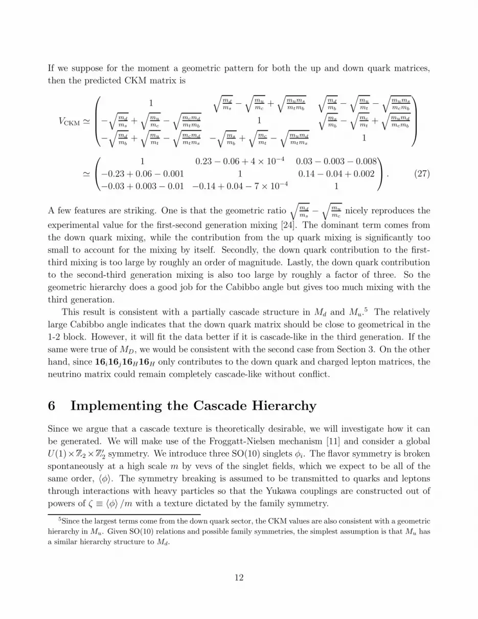
If we suppose for the moment a geometric pattern for both the up and down quark matrices,

then the predicted CKM matrix is

VCKM ≃

1√

md

ms−

√

mu

mc+

√

mums

mtmb

√

md

mb−

√

mu

mt−

√

mums

mcmb

−√

md

ms+

√

mu

mc−

√

mcmd

mtmb1

√

ms

mb−

√

mc

mt+

√

mumd

mcmb

−√

md

mb+

√

mu

mt−

√

mcmd

mtms−

√

ms

mb+

√

mc

mt−

√

mumd

mtms1

≃

1 0.23 − 0.06 + 4 × 10−4 0.03 − 0.003 − 0.008

−0.23 + 0.06 − 0.001 1 0.14 − 0.04 + 0.002

−0.03 + 0.003 − 0.01 −0.14 + 0.04 − 7 × 10−4 1

. (27)

A few features are striking. One is that the geometric ratio√

md

ms−

√

mu

mcnicely reproduces the

experimental value for the first-second generation mixing [24]. The dominant term comes from

the down quark mixing, while the contribution from the up quark mixing is significantly too

small to account for the mixing by itself. Secondly, the down quark contribution to the first-

third mixing is too large by roughly an order of magnitude. Lastly, the down quark contribution

to the second-third generation mixing is also too large by roughly a factor of three. So the

geometric hierarchy does a good job for the Cabibbo angle but gives too much mixing with the

third generation.

This result is consistent with a partially cascade structure in Md and Mu.5 The relatively

large Cabibbo angle indicates that the down quark matrix should be close to geometrical in the

1-2 block. However, it will fit the data better if it is cascade-like in the third generation. If the

same were true of MD, we would be consistent with the second case from Section 3. On the other

hand, since 16i16j16H16H only contributes to the down quark and charged lepton matrices, the

neutrino matrix could remain completely cascade-like without conflict.

6 Implementing the Cascade Hierarchy

Since we argue that a cascade texture is theoretically desirable, we will investigate how it can

be generated. We will make use of the Froggatt-Nielsen mechanism [11] and consider a global

U(1)×Z2×Z′2

symmetry. We introduce three SO(10) singlets φi. The flavor symmetry is broken

spontaneously at a high scale m by vevs of the singlet fields, which we expect to be all of the

same order, 〈φ〉. The symmetry breaking is assumed to be transmitted to quarks and leptons

through interactions with heavy particles so that the Yukawa couplings are constructed out of

powers of ζ ≡ 〈φ〉 /m with a texture dictated by the family symmetry.

5Since the largest terms come from the down quark sector, the CKM values are also consistent with a geometric

hierarchy in Mu. Given SO(10) relations and possible family symmetries, the simplest assumption is that Mu has

a similar hierarchy structure to Md.

12

We assign the following charges:

Field 161 162 163 10H φ1 φ2 φ3

U(1) 2 1 0 0 −1 0 0

Z2 − − + + + − +

Z

′2 − + + + + + −

Then the operator M ij1016i16j10H originates from Φij16i16j10H , where Φ represents the higher-

dimensional couplings,

Φ =

1

m4 (φ1)4 1

m4 (φ1)3 φ3

1

m4 (φ1)2 φ2 φ3

1

m4 (φ1)3 φ3

1

m2 (φ1)2 1

m2 φ1 φ2

1

m4 (φ1)2 φ2 φ3

1

m2 φ1 φ2 1

, (28)

so that

M10 ∼

ζ4 ζ4 ζ4

ζ4 ζ2 ζ2

ζ4 ζ2 1

. (29)

This is the cascade form of Eq. (22) with η = ζ4 and ǫ = ζ2. The same pattern can easily be

reproduced in the other operators which contribute to fermion masses. Note that in the absence

of the Z2 symmetries we would have generated a geometric hierarchy.

We must also consider whether a cascade hierarchy can naturally accommodate the fermion

masses in a unified theory. Restricting ourselves to two generations, the operators discussed in

Section 2 contribute to the (normalized) mass matrices as follows:

Mu =

(

α′ α + β

α − β 1

)

, MD =

(

α′ α − 3β

α + 3β 1

)

,

Md =

(

α′ + γ′ α + β + γ

α − β + γ 1

)

, Me =

(

α′ + γ′ α − 3β + γ

α + 3β + γ 1

)

. (30)

Here, the terms α and α′ parameterize the operator 16i16j10H . The parameter β derives from

16i16j10H45H , while γ and γ′ characterize 16i16j16H16′H . Looking at the determinants, we

calculate the mass ratios:

mc

mt

≃∣

∣α′ − α2 + β2∣

∣ , ǫ ≃∣

∣α′ − α2 + 9β2∣

∣ ,

ms

mb≃

∣

∣α′ + γ′ + β2 − (α + γ)2∣

∣ ,mµ

mτ≃

∣

∣α′ + γ′ + 9β2 − (α + γ)2∣

∣ . (31)

As expected, β accounts for the difference of down quark and charged fermion masses,

8β2 =mµ

mτ∓ ms

mb≃

{

4 × 10−2 −8 × 10−2 +

(32)

13

where we used (mµ/mτ )GUT≃ 0.06 and (ms/mb)GUT

≃ 0.02. Since we wish to minimize off-

diagonal terms in a cascade-like matrix, we will use the smaller value for β,6

β ≃ 7 × 10−2 . (33)

Then we obtain

ǫ =mc

mt

+ 8β2 ≃ 7 × 10−2 , (34)

with (mc/mt)GUT≃ 0.03.

In order to have a cascade form for MD, we require α′ ∼ α ± 3β ∼ ǫ. Since 3β ≃ 0.2, this

implies α′ ∼ 0.1, independent of α. This value of α′ can be consistent with the value of ǫ in

Eq. (34), but it needs to cancel significantly with α2 to ensure a suitably small value for mc/mt.

Conversely, mc/mt implies α′ . 10−2, which leads to a geometric hierarchy in MD. Since we

have been trying to avoid requiring the cancellation of theoretical parameters, this simple cascade

ansatz is problematic.

One particularly attractive way out of this dilemma is to consider the possibility that MD,

but not Mu, receives additional contributions, e.g., via particular higher-dimensional operators.

If such an operator gave a contribution to the (22)-element of MD of order ǫ ∼ 0.1, α′ could be

made sufficiently small. We consider such a scenario in the following section.

7 New Contributions to MD

In Section 4 we saw that the observed pattern of neutrino masses and mixings leads us to an

enhanced hierarchy for MR, compared to MD. One should note, however, that while MD is related

to the observed quark and charged lepton hierarchies by SO(10) and any family symmetries, it

is not directly observed. In particular, one may include another operator, 16i16j16H16′H . As

noted above, the weak doublet in 16′H can acquire a weak scale vev u′ such that this operator

potentially contributes to the up quark and neutrino masses. However, it can be constructed to

contribute only to the Dirac neutrino matrix. In this case we expect u′ < u, since u is required

to generate a large top quark mass and the sum of the squares of weak scale vevs must equal

(246 GeV)2.

A simple possibility for generating this operator is to integrate out SO(10) singlets, S, at

some scale above the relevant GUT scale vevs. For this purpose we can propose the operators

M ij16i16HSj + M′ij16i16

′HSj + ms (MS)ij SiSj . (35)

We assume at least three singlets to guarantee that all three righthanded neutrinos become heavy.

As usual, we define ms to have units of mass so that MS is dimensionless with entries of order

1 or smaller, and similarly we normalize M and M′in Eq. (38). In the following analysis we

6The larger value, β ≃ 0.1, leads to ǫ ≃ 0.1.

14

assume that all the S singlets are integrated out to generate an effective Majorana mass for the

N ’s. To compute this via a straightforward seesaw mechanism, we will work in the basis where

MS is diagonal and impose the conditions

(MS)ii >v

ms(36)

for all i.

The mass matrix for the electrically neutral particles reads7

(

ν N S)

0 1

2uMD

1

2u′M

′

1

2uMT

D 0 1

2vM

1

2u′M

′T 1

2vM

TmsMS

ν

N

S

. (37)

As derived in Appendix A, the light neutrino mass matrix is then given by

Mν ≃ MD

(

M−1

)T

MSM−1

MTD − x

2

[

M′M

−1

MTD + MD

(

M′M

−1)T

]

, x ≡ u′v

u ms≪ 1 . (38)

The mass of the heaviest neutrino is of order u2ms/v2. It is crucial that, in the final formula,

MD appears in all terms, i.e., terms quadratic in M′M

−1

have not appeared.

Let us study the effect of the new contributions. We parameterize the various matrices as

follows:

M−1

R =(

M−1

)T

MSM−1 ≡

A B C

B D E

C E F

, M′M

−1

=

a b c

b′ d e

c′ e′ f

, (39)

(note that the matrix M′M

−1

is generally not symmetric), and

M−1

D Mν

(

M−1

D

)T= M−1

R − x

2

[

M−1

D M′M

−1

+(

M′M

−1)T

(

M−1

D

)T]

=

A′ B′ C ′

B′ D′ E ′

C ′ E ′ F ′

(40)

The last matrix, with primed capital letters, is the total effective matrix which takes the place of

M−1

R in Section 4. The unprimed capital letters parameterize the familiar heavy neutrino matrix

and the lower case letters parameterize the new terms. Before proceeding to consider the effects

of these new terms, we note that MR can easily acquire a double hierarchy if it is generated by

integrating out heavy singlets, as described above. If M has a hierarchy comparable to MD and

MS is roughly democratic, a double hierarchy occurs naturally.

We can write the total effective parameters in terms of these old and new components and

perform the same analysis on the total effective matrix (A′ − F ′) as we did on the simple type-I

parameters (A − F ) in Section 4. Then we obtain the following set of equations:

A′ ≃ A +

[

a

η+ b′

µ′√

ηǫ+ c′

ν ′√

η

]

x

7Barr calls this scenario a type-III seesaw mechanism [25]; however, it can also be understood as a product of

two type-I mechanisms.

15

B′ ≃ B +1

2

[

aµ√ηǫ

+b

η+

b′

ǫ+ c′

ρ′√

ǫ+ d

µ′√

ηǫ+ e′

ν ′√

η

]

x

C ′ ≃ C +1

2

[

aν√η

+ b′ρ√ǫ

+ c′ +c

η+ e

µ′√

ηǫ+ f

ν ′√

η

]

x

D′ ≃ D +

[

bµ√ηǫ

+d

ǫ+ e′

ρ′√

ǫ

]

x

E ′ ≃ E +1

2

[

bν√η

+ cµ√ηǫ

+ dρ√ǫ

+e

ǫ+ e′ + f

ρ′√

ǫ

]

x

F ′ ≃ F +

[

cν√η

+ eρ√ǫ

+ f

]

x (41)

In these equations we have kept only the leading terms. In doing so, we make use of the

important fact that the constraints on µ, ν, and ρ still apply. They follow from consideration of

the experimental data and the geometric constraints on MD only.8

Although these equations still appear somewhat complicated, the requirement that we fit the

same hierarchy of orders as imposed in Eqs. (18) can only be satisfied in a few ways. In general,

the new terms give us new parameters which could play a role in a precision fit to the data, but

they will not affect the conclusions of this paper unless they dominate over the old terms. Let

us consider the canonical case, which implies

A′ B′ C ′

B′ D′ E ′

C ′ E ′ F ′

∝

1

η2

1

ηǫ1

η1

ηǫ1

ǫ21

ǫ1

η1

ǫ1

. (42)

Examining Eq. (41), this puts some initial constraints on our new parameters. For example,

bx

η≤ B′ ∼ F ′

ηǫ. (43)

These constraints may be summarized in matrix form:

a b c

b′ d e

c′ e′ f

.

1

η1

ǫ1

1

η1

ǫ1

1

η1

ǫ1

F ′

x. (44)

Taking these restrictions into account, we conclude that to satisfy A′

F ′∼ 1

η2 we must have

A ∼ F ′ 1

η2or a ∼ F ′ 1

ηx. (45)

The latter case is initially appealing because one can apparently trade the strong double hierarchy

constraint on MR for a weaker standard hierarchy in M′M

−1if the term involving a dominates.

8This would not be the case if there were new terms in the effective total matrix which did not involve MD.

16

This turns out not to be feasible. Recall that M and M′have all entries of order 1 or less.

Thus, if a = F ′ 1

ηx, there exists some i and some n ≥ 1 for which

M′1i =

1

nand M

−1

i1 =nF ′

ηx(46)

(cf. Eq. (39)). Then the assumption that the a term dominates over A gives us the inequality

1

η2∼ ax

ηF ′ ≥A

F ′ =1

F ′

[

(

M−1

)T

MSM−1

]

11

≥(

n

ηx

)2

(MS)iiF′ , (47)

from which we obtain (MS)iiF′ ≤ x2

n2 . Applying the seesaw constraint on MS and inserting the

definition of x gives us

v

msF ′ ≤ (MS)iiF

′ ≤ u′2v2

n2u2m2s

. (48)

This requires F ′ to be too small, that is,

1 .

[

(

M−1

)T

MSM−1

]

33

= F ≤ F ′ ≤ u′2v

n2u2ms. (49)

Since v ≪ ms and u′ . u, this condition cannot be satisfied. Thus the additional contributions

cannot dominate over the type-I contributions or change the need for a double hierarchy.

One can instead look at case 1 from Section 3. If the new terms dominate in the largest ratio,

which is still A′/F ′, this implies M−1

i1 = λnF ′

ηx. Proceeding as in the canonical case above, one

finds λ(MS)iiF′ ≤ x2

n2 . Since we require F ′ ≥ 1 this is only possible if

x2 ≥ (MS)iiλn2 ≥ v

msλn2 , (50)

or equivalently,

λ ≤ u′2v

n2u2ms≪ 1. (51)

This is a very marginal case since we are relying on v ≪ ms to use the seesaw formula as a valid

approximation and λ ∼ 0.2.

If we proceed nonetheless, then we impose the conditions on B′:

λ

ηǫ∼ B′

F ′ ≥B

F ′ ∼1

F ′

∑

k

M−1

k1M

−1

k2, (52)

which implies the constraint M−1

i2 ≤ x/ [nǫ(MS)ii]. Now we turn to D′ ∼ 1

ǫ2. By similar reasoning

as in the canonical case it can be shown that D must dominate to satisfy D′ of the appropriate

magnitude, due to the suppression of the new terms by x. Then

1

ǫ2∼ D′

F ′ ≥D

F ′ ∼(MS)jj

F ′

(

M−1

j2

)2

, (53)

17

for some j 6= i, which gives us the condition

M−1

j2 ∼ 1

ǫ

√

F ′

(MS)jj

. (54)

This in turn implies

M−1

j1 ≤ λ

η

√

F ′

(MS)jj, (55)

so as not to violate the bound on b. We find then that the new contributions can technically

dominate in the (11) entry but the type-I terms remain comparable and dominate in other entries,

still exhibiting a strong hierarchy compared to MD.

The related case 2, with (Mν)11 ≪ λ, is, not surprisingly, similar. One finds that the new

term a can dominate if λ√

ηǫ≤ u′2v

n2u2ms, which provides somewhat more room for consistency with

the seesaw approximation. The constraints on the matrices are

M−1

i1 ≃ λnF ′

x√

ηǫ, M

−1

i2 ≤ x

n√

ηǫ (MS)ii

, M−1

j2 ≃ 1

ǫ

√

F ′

(MS)jj, M

−1

j1 ≤ λ

η

√

F ′

(MS)jj. (56)

In both cases the new terms can dominate in some entries, but the type-I terms remain

important and retain a strong, albeit not quite double, hierarchy. We note that this is due largely

to the structure of the theory: if MR is a dimension-five operator generated by integrating out

singlets, then a hierarchy in M similar to that in MD naturally leads to a doubled hierarchy in

MR. Due to the suppression of the new terms by v/ms, MR will always play an important role.

It is interesting that even with the 16i16j16H16′H operator only contributing to the neutrino

sector, we still derive the cascade constraints. Although this operator only contributes to the

Dirac neutrino matrix, the constraints apply to the operators which generate the up quark matrix.

This follows from the precise relations between the higher dimensional operators induced by their

common origin. These relations result in MD appearing in all terms of the formula for Mν . As

a consequence of the persistent cascade constraints, we cannot use the new terms to solve the

mass splitting problems discussed in Section 6.

If one treats 16i16j16H16′H and 16i16j16H16H as independent, it is possible to relax said

constraints. That is, in the discussion above both operators depend on the coupling M ij16i16HSj

and are therefore related. If we allow them to vary arbitrarily, then the modified seesaw formula

in Eq. (38) would have additional terms which did not involve MD. In effect, we would be adding

new terms to the Dirac neutrino matrix which could strongly alter its hierarchy compared to the

quarks and charged leptons. If this resulted in a relatively weak Dirac neutrino hierarchy, MR

would have a correspondingly weakened hierarchy and the mixing parameter constraints would

also weaken. However, as shown above, this is not necessarily the case when one begins with a

more complete theory.

18

In general, if one can weaken the Dirac neutrino hierarchy without upsetting the charged

fermion hierarchies, the requirement of a double hierarchy in MR and a cascade hierarchy in

MD becomes less restrictive, since they are specified relative to the eigenvalue hierarchy of MD.

One possibility for doing so may be to introduce a vector-like fourth generation of down quarks

and leptons at the GUT scale. This can relate MD to the down quark hierarchy such that the

hierarchy of MR is similar to that of the up quarks [26].

8 Lopsided Models

Thus far, we have not allowed for any cancellations between terms in our equations, in keeping

with our aim to eliminate unnatural models. There are, however, two scenarios where one must

be more careful. These are cases where unitary rotations play a very significant role either due

to large rotations or small entries in the neutrino matrix.

In this section we will consider the first type of these cases, lopsided models, wherein the

operator 16i16j16H16′H is constructed so as to contribute in a highly asymmetrical way to the

down quark and charged lepton mass matrices [7].9 These lopsided matrices can yield a natural

hierarchy while violating the geometric pattern limit discussed above. Lopsidedness results in

large off-diagonal terms in the unitary rotations on one side of the matrix but not both.

To illustrate these features we will restrict ourselves to two generations first. The follow-

ing table summarizes the three natural cases we have discussed for a generic matrix M with

eigenvalues ǫ and 1, which is diagonalized by the unitary rotation matrices L and R.

Hierarchy M L R

Geometric(

ǫ√

ǫ√ǫ 1

) (

1√

ǫ√ǫ 1

) (

1√

ǫ√ǫ 1

)

Cascade ( ǫ ǫǫ 1 ) ( 1 ǫ

ǫ 1) ( 1 ǫ

ǫ 1)

Lopsided ( ǫ ǫ1 1 ) ( 1 ǫ

ǫ 1) ( 1 1

1 1)

For both the geometric and cascade cases L and R are similar to each other. As expected, the

off-diagonal entries of L and R for the cascade case are smaller than in the geometric case.

The lopsided case, being highly asymmetric, leads to very different rotation matrices on the

left and right. We see that to generate large mixing on one side, i.e., R with all entries of the

same order, we are led to L being closer to diagonal than in the geometric case. Rather, it is

similar to the cascade rotation matrices. So in this simple case, to preserve naturalness, there is

a tradeoff between the left and right sides. If one side’s unitary rotation violates the geometric

naturalness bound, the other’s is concomitantly constrained to be closer to unity.

To take potentially large mixing in the charged lepton sector into account, we have to reeval-

uate our seesaw formula. In Eq. (12), we neglected the rotations from the charged lepton sector,

9We will not discuss the origin of these lopsided matrices, which, e.g., can be due to family symmetries [7].

19

parameterized by Le (cf. Eq. (7)). To include them we rewrite the formula as

R†DM−1

R R∗D = D−1

D V0M′νV

T0

D−1

D , (57)

where

M ′ν ≡ VPMNSDνV

TPMNS = L†

eMνL∗e, V0 ≡ L†

DLe . (58)

M ′ν is the light neutrino mass matrix in the basis where the charged leptons are diagonal. It can

have the same forms as discussed in Section 3 for Mν . With the substitutions Mν → M ′ν and

LD → V0, the equations used above are unaltered.

The crucial difference is that the assumed form of LD in Eq. (3) does not necessarily apply

to V0 in the lopsided case. Since V0 contains off-diagonal entries of order one, we may arrange

for terms of equal order to cancel each other in V0M′νV

T0 . This is not fine tuning because

we are, in effect, canceling an experimental term with a theoretical one, rather than canceling

two theoretical parameters against each other. To put it another way, we are simply using a

theoretical term to generate an experimental parameter of the same order. The result is that

we may be able to have a form for R†DM−1

R R∗D which does not have such a strong hierarchy, and

which in turn may not imply the restrictive cascade form for MD. In such a scenario, some or

all of the large mixing in VPMNS comes from charged lepton unitary rotations.

To examine the lopsided case further we must see what can be said about the matrix V0.

Again, we can look at the CKM matrix for possible constraints. It can tell us about the potential

lopsidedness in the down quark and charged lepton mass matrices. The operator we are using to

generate lopsidedness contributes to Me as the transpose of its contribution to Md, as is familiar

from SU(5) models.10 Hence, large rotations in Le would coincide with large rotations in Rd and

vice versa. We now see that the experimental values are consistent with either a cascade structure

or a lopsided structure for the down quark mass matrix in the third generation couplings.

One might hope that the relatively large 1-2 mixing, which is consistent with a geometric

hierarchy in the down quark matrix (cf. Section 5), would constrain the 1-2 mixing in Rd. This,

however, turns out not to be the case. We can construct a matrix with all the desired features

and generically large righthanded mixing, e.g.,

Md ∼

md

mb

√mdms

mb

md

mb√

mdms

mb

ms

mb

ms

mb

1 1 1

, Ld ∼

1√

md

ms

√mdms

mb√

md

ms1 ms

mb√

mdms

mb

ms

mb1

, Rd ∼

1 1 1

1 1 1

1 1 1

. (59)

Thus, although the CKM matrix is highly suggestive of either a partially cascade or lopsided form

for the down quark mass matrix, it is difficult to constrain the form of Rd and its counterpart

Le in the latter case.

10This is simply due to the fact that 16H breaks SO(10) to SU(5), so 16i16j16H16′

H is basically an SU(5)

Yukawa operator for down quarks and charged fermions, suppressed by v/M .

20

On the other hand, we note that since VPMNS has a small value for the (13) entry, naturalness

requires that at least one entry in the column Li1e be correspondingly small. This suggests that

we can rule out the extreme lopsided case shown above.

Lopsidedness also modifies the eigenvalue fitting we did in Section 6. Let us consider the case

where 16i16j16H16′H is lopsided and assume that it contributes to only one off-diagonal entry

in Md and Me in a significant way. Then the mass matrices in Eq. (30) are modified to

Md =

(

α′ + γ′ α + β

α − β + γ 1

)

, Me =

(

α′ + γ′ α − 3β + γ

α + 3β 1

)

, (60)

with the corresponding eigenvalues

ms

mb=

∣

∣

∣

∣

α′ + γ′ + β2 − α2 − γ (α + β)

1 + γ2

∣

∣

∣

∣

,mµ

mτ=

∣

∣

∣

∣

α′ + γ′ + 9β2 − α2 − γ (α + 3β)

1 + γ2

∣

∣

∣

∣

. (61)

This yields

mµ

mτ

− ms

mb

=2β (4β − γ)

1 + γ2

γ∼1−−→ β ∼ 4 × 10−2 , (62)

which is only a slight improvement over the symmetric case, a cascade structure in MD is still

inconsistent with the charged fermion hierarchies. Thus, in the absence of additional contribu-

tions to the mass matrices, it seems we must rely on large, lopsided mixing between the second

and third generations to alleviate the need for a cascade structure in the 2-3 block of MD.

9 Small Entries and Mixing

Aside from lopsided matrices, there is another scenario in which V0 can play an important role.

We saw in Section 4 that the entries of the first row and column of R†DM−1

R R∗D are smaller in

the cases 1 and 2. If we allow cancellations between these entries of order λ and the mixing

parameter µ′√ηǫ, we might expect some qualitatively different results. In this more general case,

we use µ′, ν ′ and ρ′ to parameterize V0 rather than LD. Including the effects of Le, we no longer

have the symmetry constraints (µ, ν, ρ) ∼ (µ′, ν ′, ρ′).

We consider case 1:

R†DM−1

R R∗D ∼

λη2

1

ηǫ

(

λ + µ′√ηǫ

)

1

η

(

λ + µ′√ηǫ

)

1

ηǫ

(

λ + µ′√ηǫ

)

1

ǫ21

ǫ1

η

(

λ + µ′√ηǫ

)

1

ǫ1

.

Here, although the unitary rotations remain relatively close to unity, the rotation parameter

µ′√ηǫ

may be large enough to cancel the experimental term λ. Such cancellation is only possible

if µ′ ∼ 1.11 Under geometrical constraints, the (11) entry will be λη2 , while the (12) entry could be

11Since µ′ includes contributions from Le, its coefficient√

η/ǫ should be√

me/mµ if the charged lepton ratio

is larger. However, since√

me/mµ ∼ 0.1 ∼√

η/ǫ under our assumptions, we keep our familiar notation.

21

much smaller than ληǫ

. One can proceed to analyze the mixing parameters in RD as in Section 4.

Due to the relatively large (11) entry, one finds that the constraints

µ .

√

η

ǫ

(

1 +µ′

λ

√

η

ǫ

)

, ν .√

ν

(

1 +µ′

λ

√

η

ǫ

)

, ρ .√

ǫ, (63)

are required to preserve the small (12) and (13) entries. Since this requires µ ≪ µ′ ∼ 1, the

charged lepton rotations would have to be significantly larger than those from the Dirac neutrino

matrix, at least for the 1-2 mixing. This would suggest an approximately geometric structure in

the charged lepton matrix and a Dirac neutrino matrix with very small first generation mixing.

Thus, the Dirac neutrino matrix would have a more restricted form than the cascade hierarchy

derived for the simpler case without cancellations. Unless some additional information prompts

us to favor these textures for Mν , MD and Me, there is no compelling reason to further pursue

this route.

In the second case, where (Mν)11 ∼ 0, we find that the constraints are the same as those

listed in Eq. (25), i.e., the same as we found for this case without allowing for cancellations.

These results hold because, regardless of how small λ + µ′√ηǫ

may be, we retain the same

relative hierarchy between the first generation entries and the same hierarchy in the 2-3 block,

cf. Eq. (15).

We conclude that these potential cancellations have little effect on our previous considerations.

10 Outlook

Barring cancellations or additional flavor symmetries, the observed pattern of neutrino mass

splittings and mixing angles leads us to two related propositions for simple model building in

the general context of a grand-unified theory with type-I seesaw mechanism. The first is a

double hierarchy, with respect to the hierarchy of the Dirac matrix, MD, in the effective heavy

neutrino matrix MR. The second, contingent upon the first, is a cascade structure in MD, or a

texture which is even closer to diagonal. These conclusions follow only from the structure of the

type-I seesaw formula, together with the observation that the experimental neutrino data most

naturally arise from an approximately democratic effective light neutrino matrix. If the neutrino

masses obey a normal hierarchy, i.e., m1 . m2 ∼√

∆m2

sol≪ m3 ∼

√

∆m2atm, it is possible to

relax these constraints, but it remains true that MR should have an enhanced hierarchy and MD

should have a sub-geometrical structure. Moreover, in this case some approximate symmetry

must exist to generate a second large mixing angle and a hierarchy consistent with experiment.

These conclusions are rather general and not restricted to the specific model with small

representations outlined in Section 2. They hold for hierarchical, symmetric matrices, up to

factors of order one. In light of the quark and charged lepton mass hierarchies, it is natural for

MD to be hierarchical. In particular, this matrix is closely related to the up quark matrix in

many GUT models. Family symmetries will also tend to engender such relations. In Section 7

22

we showed that even adding an operator which ostensibly only contributes to the Dirac neutrino

matrix does not necessarily relax our conclusions.

Can we implement these textures in a complete model? We discussed a scenario with a

U(1) ×Z2 ×Z2 flavor symmetry, where we generated a cascade structure for the Dirac matrices

through the Froggatt-Nielsen mechanism. A double hierarchy in MR is natural if it is an effective

operator generated by integrating out singlets coupled to 16i16H , where this coupling has an

eigenvalue hierarchy similar to that in MD (cf. Ref. [22]). However, this structure led to problems

in the quark sector. We have seen that the relatively large Cabibbo angle implies that the down

quark matrix is not purely cascade-like, although a cascade structure in the third generation is

supported. This does not necessarily conflict with a fully cascade pattern in MD, but it requires

a somewhat more complicated picture than the simple model described above. Furthermore,

in our specific model, we rely on the antisymmetric operator 16i16j10H45H to differentiate the

down quark and charged lepton matrices. This implies that its contributions cannot be too small.

Since it also contributes to the up-quark and neutrino matrices, it becomes difficult to reconcile

a cascade structure in these matrices with the strong up-quark hierarchy in a natural way.

Lopsided models may provide us a way out of these potential difficulties. Compared with

a cascade pattern, they are equally compatible with the CKM matrix. For the purposes of

mass fitting, lopsidedness slightly relaxes the need for large off-diagonal contributions from

16i16j10H45H . More importantly, a lopsided charged lepton matrix introduces large rotations

which contribute to the PMNS matrix. If these are primarily responsible for one or both of the

large mixing angles, it is possible to reduce the pull towards a double hierarchy in MR. This in

turn can relax the constraints that lead us to a cascade structure for MD and so for Mu. Exactly

how much lopsidedness can obviate the need for a double hierarchy remains an open question.

The atmospheric mass splitting remains small compared to the quark mass splittings, irrespec-

tive of the origin of the large mixing angles. This will tend to require an enhanced hierarchy in

at least part of MR. Additionally, while it is technically possible that most or all of the PMNS

structure comes from charged lepton rotations, we must ask how much can be done in a natural

way. For example, as discussed at the end of Section 8, a small value for θ13 precludes generically

large mixing from lopsidedness in all generations.

This brings us to the nature and origin of θ13 in general, which we have not addressed in detail

in this paper. We chose to leave this an open question in light of the current uncertainty in the

size of θ13: only an upper bound is known. While it is clear that the solar and atmospheric mixing

angles are large compared with those in the quark sector, θ13 may or may not be comparatively

small. Actually, the experimental upper limit, approximately 10◦, is of the same order as the

Cabibbo angle. This is large enough that its smallness compared to the other neutrino angles

may be explained by normal fluctuations of order one parameters without violating our sense of

naturalness [6]. However, if θ13 is significantly closer to zero we should seek some more robust

explanation. For the forms of Mν listed in Section 3, this would require a symmetry closely

relating various matrix elements. Another possibility arises for partially lopsided matrices: if

one large mixing angle arises from the charged lepton sector and the other from Mν then it is

23

natural to preserve a small third angle. Clearly, it is important to determine the order of θ13.

In summary, a combination of partially lopsided and partially cascade matrices, in conjunction

with an enhanced hierarchy in MR, seems to be the most natural route to explain the generic

features of the quark and lepton data in a grand-unified model. The details of a complete model

remain to be worked out, but our conclusions follow from a fairly general framework. It will be

interesting to see if a workable model can be obtained with relatively simple family symmetries

and what consequences there might be for experimental predictions.

We would like to thank S. Willenbrock for useful comments on the manuscript. This work was

supported in part by the U. S. Department of Energy under contract No. DE-FG02-91ER40677,

as well as the Sonderforschungsbereich Transregio 9 Computergestutzte Theoretische Teilchen-

physik of the Deutsche Forschungsmeinschaft.

A Derivation of Expanded Seesaw Formula

In this appendix, we derive the extended seesaw formula, given in Eq. (38). As mentioned in

Section 7, it is crucial that terms quadratic in M′M

−1

do not appear. The formula was originally

derived in Ref. [25] through a slightly different calculation.

As displayed in Eq. (35), we propose the operators

WS = M ij16i16HSj + M′ij16i16

′HSj + ms (MS)ij SiSj .

We integrate out the singlet fields, S, by taking a partial derivative and setting it equal to zero,

∂WS

∂Sj≡ 0 : Si = − 1

2 ms

[

M ij16i16H + M′ij16i16

′H

]

(

M−1

S

)

jk. (64)

Plugging this into our initial equation yields

W eff

S = − 1

4ms

16i

[

(

MM−1

S MT)

ij16H16H +

(

M′M−1

S M′T

)

ij16

′H16

′H

+ 2(

M′M−1

S MT)

ij16H16

′H

]

16j . (65)

Now we let the Higgs fields acquire their GUT and weak scale vevs and we include the Dirac

term νMDN , where ν and N are the left and right-handed neutrinos, respectively. Suppressing

the generation indices, we obtain

WN = − 1

4ms

[

v2 N(

MM−1

S MT)

N + u′2 ν(

M′M−1

S M′T

)

ν + 2 u′v ν(

M′M−1

S MT)

N]

+ u ν MD N , (66)

We extremize with respect to N and find

∂WN

∂N≡ 0 : N =

[

u ms

v2MD

(

M−1

)T

MSM−1 − u′

vM

′M

−1

]

ν . (67)

24

Inserting this into the last equation and performing a little algebra gives the amended seesaw

formula

W eff

ν ≃{

MD

(

M−1

)T

MSM−1

MTD − 1

2

u′v

ums

[

M′M

−1MT

D + MD

(

M′M

−1)T

]}

u2ms

v2. (68)

References

[1] W. M. Yao et al. [Particle Data Group], J. Phys. G 33, 1 (2006).

[2] A. Strumia and F. Vissani, arXiv:hep-ph/0606054.

[3] P. Minkowski, Phys. Lett. B 67, 421 (1977).

[4] H. Georgi, in: Particles and fields (ed. C. Carlson), AIP Conf. Proc. 23, 575 (1975);

H. Fritzsch and P. Minkowski, Annals Phys. 93 (1975) 193.

[5] R. N. Mohapatra and A. Y. Smirnov, Ann. Rev. Nucl. Part. Sci. 56, 569 (2006);

G. Altarelli, arXiv:0705.0860 [hep-ph].

[6] G. Altarelli and F. Feruglio, New J. Phys. 6, 106 (2004).

[7] C. H. Albright and S. M. Barr, Phys. Rev. D 62, 093008 (2000); Phys. Rev. D 64, 073010

(2001).

[8] see e.g., K. S. Babu, J. C. Pati and F. Wilczek, Nucl. Phys. B 566, 33 (2000);

R. Dermisek and S. Raby, Phys. Rev. D 62, 015007 (2000);

T. Blazek, S. Raby and K. Tobe, Phys. Rev. D 62, 055001 (2000);

J. Sayre and S. Wiesenfeldt, Phys. Lett. B 637, 295 (2006).

[9] K. S. Babu and R. N. Mohapatra, Phys. Rev. Lett. 74, 2418 (1995).

[10] I. Dorsner and S. M. Barr, Nucl. Phys. B 617, 493 (2001).

[11] C. D. Froggatt and H. B. Nielsen, Nucl. Phys. B 147, 277 (1979).

[12] G. Anderson, S. Raby, S. Dimopoulos, L. J. Hall and G. D. Starkman, Phys. Rev. D 49,

3660 (1994);

S. Wiesenfeldt and S. Willenbrock, Phys. Lett. B 661, 268 (2008).

[13] For a recent brief review, see A. Melfo, AIP Conf. Proc. 917, 252 (2007).

[14] J. Lesgourgues and S. Pastor, Phys. Rept. 429, 307 (2006);

S. Hannestad and G. G. Raffelt, JCAP 0611, 016 (2006).

[15] L. Baudis et al., Phys. Rev. Lett. 83, 41 (1999);

H. V. Klapdor-Kleingrothaus et al., Eur. Phys. J. A 12, 147 (2001).

[16] P. F. Harrison, D. H. Perkins and W. G. Scott, Phys. Lett. B 530, 167 (2002).

[17] S. Antusch, J. Kersten, M. Lindner, M. Ratz and M. A. Schmidt, JHEP 0503, 024 (2005).

25

[18] H. Harari, H. Haut and J. Weyers, Phys. Lett. B 78, 459 (1978);

L. Lavoura, Phys. Lett. B 228, 245 (1989);

H. Fritzsch and J. Plankl, Phys. Lett. B 237, 451 (1990).

[19] H. V. Klapdor-Kleingrothaus and I. V. Krivosheina, Mod. Phys. Lett. A 21, 1547 (2006).

[20] See also C. Arnaboldi et al., arXiv:0802.3439 [hep-ex].

[21] G. Altarelli, F. Feruglio and I. Masina, Phys. Lett. B 472, 382 (2000).

[22] R. Dermisek, Phys. Rev. D 70, 073016 (2004).

[23] J. A. Casas, A. Ibarra and F. Jimenez-Alburquerque, JHEP 0704, 064 (2007).

[24] H. Fritzsch, Phys. Lett. B 70, 436 (1977).

[25] S. M. Barr, Phys. Rev. Lett. 92, 101601 (2004).

[26] Y. Nomura and T. Yanagida, Phys. Rev. D 59, 017303 (1999);

T. Asaka, Phys. Lett. B 562, 291 (2003);

W. Buchmuller, L. Covi, D. Emmanuel-Costa and S. Wiesenfeldt, JHEP 0712, 030 (2007).

26