JHEP06(2013)097

Published for SISSA by Springer

Received: March 8, 2013

Revised: May 27, 2013

Accepted: May 29, 2013

Published: June 25, 2013

Neutrino mass matrix textures: a data-driven

approach

E. Bertuzzo,a P.A.N. Machadoa,b,c and R. Zukanovich Funchala,b

aInstitut de Physique Theorique,

CEA-Saclay, 91191 Gif-sur-Yvette, FrancebInstituto de Fısica, Universidade de Sao Paulo,

C. P. 66.318, 05315-970 Sao Paulo, BrazilcTH Division, Physics Department, CERN,

CH-1211 Geneva 23, Switzerland

E-mail: enrico.bertuzzo@cea.fr, accioly@fma.if.usp.br,

zukanov@if.usp.br

Abstract: We analyze the neutrino mass matrix entries and their correlations in a

probabilistic fashion, constructing probability distribution functions using the latest results

from neutrino oscillation fits. Two cases are considered: the standard three neutrino

scenario as well as the inclusion of a new sterile neutrino that potentially explains the

reactor and gallium anomalies. We discuss the current limits and future perspectives on

the mass matrix elements that can be useful for model building.

Keywords: Beyond Standard Model, Neutrino Physics, Standard Model

ArXiv ePrint: 1302.0653

Open Access doi:10.1007/JHEP06(2013)097

JHEP06(2013)097

Contents

1 Introduction 1

2 Reconstructing the neutrino mass matrix from experimental data 2

3 The standard scenario 3

3.1 Correlations among matrix elements 4

3.1.1 Hierarchical case 4

3.1.2 Quasi-degenerate case 7

3.1.3 Future perspectives 8

4 The 3+1 scenario 12

5 Final discussion and conclusion 15

A Matrix elements squared 17

B Complete set of correlation plots for the matrix elements 21

1 Introduction

The year 2012 represents a milestone in neutrino physics. Thanks to the measurement

of the last mixing angle of the standard neutrino oscillation scenario, θ13, by the reactor

experiments Double-CHOOZ [1], Daya-Bay [2] and RENO [3] (after the first positive ev-

idence from accelerators [4, 5]), the mixing in the leptonic sector is starting to shape up.

The impact of a rather unexpectedly large mixing angle θ13 is twofold: it promotes the

discovery of CP violation in the neutrino sector to a yet daunting but conceivable task, and

at the same time it proves that the description of neutrino oscillation data must involve all

three Standard Model neutrino flavors.

Hints of the sensitivity to CP phases are already showing their first signs when we

combine accelerator νµ → νe with reactor νe → νe data [8], or when we perform global

fits [9–11]. Furthermore, the combined fit of neutrino oscillation data shows for the first

time a very precise and almost complete determination of the parameters that enter the

standard neutrino oscillation scheme. In fact, in spite of the unknowns (neutrino mass

hierarchy, absolute neutrino mass scale, CP phases and the correct octant for θ23) all

measured parameters, with the exception of sin2 θ23, are now so well determined that it is

enough to quote them by giving the best fit value with the 1 σ uncertainty.

However, not all neutrino data can be explained by this standard scenario of three

flavor neutrinos. In fact, along the years a number of so-called anomalies have crept

into the picture. First, the excess of νe events in the νµ → νe mode observed by the short

– 1 –

JHEP06(2013)097

baseline LSND [12, 13] experiment, now also supported by MiniBOONE data [14], gave rise

to the long-standing LSND anomaly. Second, the deficit of νe compared to expectations

observed by the source calibration experiments performed in the gallium radiochemical

solar neutrino detectors GALLEX [15–17] and SAGE [18–20]. This is the so-called gallium

anomaly. Third, and more recently, a re-evaluation of the reactor νe flux [21, 22] resulted

in an increase of the total flux by 3.5%. While this increase has essentially no impact on

the results of long baseline experiments, it induces a deficit of about 5.7% in the observed

event rates for short baseline (< 100 m) reactor neutrino experiments. This problem has

been referred to as the reactor antineutrino anomaly [23].

There are attempts in the literature that try to explain some or all of these anomalies

by extending the standard picture to include one or more sterile neutrinos [24–26]. These

extensions, as a rule, cannot make appearance and disappearance experiments compati-

ble. However, if one disregards the anomaly connected with the appearance experiments

LSND/MiniBOONE (for instance, assuming it is not due to oscillations), it is possible to

construct a coherent picture of all solar, atmospheric, reactor and accelerator neutrino os-

cillation data adding one extra sterile neutrino to the standard framework. This constitutes

what has been known as the 3+1 scenario.

Given the current status of the mixing parameters measurements, and in view of

the progress expected in the near future, we think it is timely to analyze the possible

structures and correlations among the neutrino mass matrix elements that are compatible

with data. In this sense, we update refs. [27, 28] using the most recent available data (see

also refs. [29, 30] for related analyses). However, our analysis will be probabilistic, since

we will construct probability distribution functions for each element of the neutrino mass

matrix. We also discuss how this might change with better determination of the presently

known oscillation parameters, as well as, the Dirac CP-phase δ. We hope this can be

helpful to understand better the patterns statistically preferred by data, and serve as a

guide for model builders.

We organize our paper as follows. In section 2 we describe how we will proceed for

the construction of probability density functions (PDF) for each element of the neutrino

mass matrix and what are the assumptions in each case. In section 3 we analyze the

possible textures of the mass matrix in the standard scenario, discussing the correlations

among matrix elements in the hierarchical and almost degenerate cases. We also discuss

the future prospects for better determining these matrix elements with neutrino oscillation

and non-oscillation data, and the possible impact on the theory. In section 4 we extend

our analysis to include the possibility of a sterile neutrino with mass and mixings allowed

by the reactor and gallium anomalies. We discuss what is the mass matrix pattern in this

scenario and how different it will be from the standard case. Finally, in section 5, we make

our last comments and draw our conclusions.

2 Reconstructing the neutrino mass matrix from experimental data

To access the impact of the progress on the determination of the neutrino oscillation pa-

rameters in the last year on the knowledge of the low energy effective neutrino mass matrix,

– 2 –

JHEP06(2013)097

in a probabilistic way, we will construct a PDF for each element of the mass matrix in the

gauge basis,

mαβ =∑i

mi e−iλi U∗

αiU∗βi (2.1)

with α, β = e, µ, τ , Uαi the elements of the mixing matrix, mi the neutrino masses and λithe Majorana-type CP phases. We will use the most recent available information from the

combination of neutrino oscillation data. Without loss of generality we will take λ2 = 0 in

our parametrization.

With the exception of sin2 θ23, we will use the following best fit points for the standard

mixing parameters [10]

∆m221 = (7.50± 0.185)× 10−5 eV2

sin2 θ12 = 0.30± 0.013

∆m231 = (+2.47± 0.07)× 10−3 eV2 (normal ordering)

∆m232 = (−2.43± 0.06)× 10−3 eV2 (inverted ordering)

sin2 θ13 = 0.023± 0.0023 (2.2)

and assume these parameters to follow a normal distribution with mean at the best fit point

and standard deviation equal to the 1 σ uncertainty. We will take the unknown Dirac-type

and Majorana-type CP phases to be flat distributed between 0 and 2π. Concerning sin2 θ23,

since the distribution cannot be assumed to be normal, we will use the exact distribution

extracted from [10].

For the 3+1 scenario we will fix the squared mass difference between the sterile and

the lightest state to two different experimentally allowed values, ∆m241 = 1.71 eV2 and

∆m241 = 0.95 eV2, allowing the corresponding mixing to vary with a flat distribution inside

the ranges |Ue4|2 = 8× 10−3 − 4× 10−2 and |Ue4|2 = 8× 10−3 − 2.5× 10−2, respectively.

To construct the PDF of each mαβ we use a Monte Carlo method. For all the mixing

parameters, we generate random numbers according to their assumed distribution, and

compute all the elements of mαβ in each case. In this manner their distribution will be

naturally correlated.

Since we do not know the neutrino mass hierarchy, the correct octant for θ23 and the

absolute neutrino mass scale, we will have to analyze each case separately.

3 The standard scenario

In the standard scenario we use the standard parametrization for the mixing matrix,

U =

c12 c13 s12 c13 s13e−iδ

−s12 c23 − c12s13s23 eiδ c12 c23 − s12s13s23 eiδ c13 s23s12 s23 − c12s13c23 eiδ −c12 s23 − s12s13c23 eiδ c13 c23

, (3.1)

with sij = sin θij , cij = cos θij and δ the Dirac-type CP phase. The two additional

Majorana-type CP phases are denoted by λ1 and λ3, and the three neutrino mass eigen-

states are ordered either as m1 < m2 < m3 (normal ordering) or as m3 < m1 < m2

(inverted ordering).

– 3 –

JHEP06(2013)097

Figure 1. PDF for |mee| when m1 → 0. The “before” (“after”) distribution corresponds to the

situation before (after) the determination of sin2 θ13 by the reactor experiments.

We will study the following different cases: hierarchical with m1 → 0; hierarchical

with m3 → 0; quasi-degenerate with m1 ∼ m2 ∼ m3 ∼ 0.1 eV. There are two possible

ordering also in the quasi-degenerate case; however, we have checked that the results are

very similar. In all cases, we will show the results for the complete s223 distribution, as well

as what is obtained cutting sharply the distribution to force θ23 to lie in the first or second

octant.

In figure 1 we illustrate, for the case m1 → 0, the impact of the determination of

sin2 θ13 on the PDF of |mee|. The distribution labeled “before” (magenta) is obtained

assuming sin2 θ13 to be flat distributed between 0 and 0.04 (CHOOZ limit [31]), while

the one labeled “after” (blue) shows the current situation. The two peaks in the “after”

distribution are due to the interference between the real U2e2m2 term and the complex

U2e3m3 term (see appendix A for detailed expressions), which depends on the cosine of the

randomly distributed CP-phases. This term depends on θ13, which gives now a sizable

contribution, not being anymore compatible with zero. The distance between the peaks

depends on m3: a larger m3 would place the peaks further apart.

In figure 2 we illustrate, again for the case m1 → 0, the effect of the determination

of sin2 θ23 (with maximal mixing now disfavored), as opposed to the maximal angle case

with MINOS uncertainty (sin2 θ23 = 0.5 ± 0.1 [32]). In the two panels we show the case

of Normal (left) and Inverted (right) Hierarchy. The asymmetric two peaks structure is

due to the fact that θ12 is not maximal. A larger m3 would shift the right endpoint of the

distribution to higher values of |mµµ|, while a larger m2 would separate the two peaks.

3.1 Correlations among matrix elements

3.1.1 Hierarchical case

In the case of Normal Hierarchy with m1 → 0, m3 ≈ 0.05 eV � m2 ≈ 0.009 eV and only

two CP-phases, δ and λ3, are relevant. Due to the µ → τ symmetry, accomplished by

s23 → c23 and c23 → −s23, the PDFs for the solution in the first θ23 octant are basically

the same as for the solution in the second octant as long as we replace: |meτ | ↔ |meµ|,|mττ | ↔ |mµµ|.

– 4 –

JHEP06(2013)097

Figure 2. PDF for |mµµ| for Normal (left panel) and Inverted (right panel) Hierarchy. The

distributions are obtained using the χ2 function extracted from [10]. For comparison, in both cases

we show the corresponding distribution using MINOS uncertainty [32].

In figure 3 we show the correlations among the absolute values of some of the matrix

elements mαβ for m1 → 0. For sin2 θ23, the complete χ2 distribution of [10] is used for

the colored regions (with blue, green and red referring to the allowed region at 68.27%,

95.45% and 99.73% CL, respectively), while the dashed (dotted) lines refer to the 99.73%

allowed region obtained cutting the distribution to force θ23 to lie in the first (second)

octant. In appendix B we present a complete set of those plots, obtained constructing a

two-dimensional PDF for each pair of elements. In all cases, on the top and to the right of

each two-dimensional distribution the projected PDFs are shown. The range of the values

allowed at 95.45% CL are given in table 1.

From figures 3 and 13 we observe that |mee| is not very correlated to any other element.

However, due to θ23 the pairs |meµ| × |meτ |, |meτ | × |mµµ|, |mµµ| × |mµτ |, |mµτ | × |mττ |,|mµµ| × |mττ | and |meµ| × |mττ | are very correlated. So, for instance, if a model predicts

|meµ| ≈ 6 meV, |meτ | must be in the range 5-8 meV, while without taking into account

this correlation the allowed range would be 2.7-9.3 meV at 95.45% CL.

From the expressions for the matrix elements given in appendix A it is easy to show

that in this case:

|meµ|2 + |meτ |2 ∼ m23y

2 +m22x

2,

|mµµ| ∼ m3z2,

|mττ |2 ∼ m23(1− 2z2) + |mµµ|2,

and

|mµτ |2 + |mττ |2 ∼ m23(1− z2),

where x = sin θ12, y = sin θ13 and z = sin θ23.

Due to the prevalence of the m3 mass, the determination of sin2 θ13 with the present

uncertainty of 10% by the reactor experiments not only affected the range of |meα|, α =

e, µ, τ , but also their PDFs.

In the case of Inverted Hierarchy with m3 → 0, m1 ≈ m2 ≈ 0.05 eV and only two

CP-phases, δ and λ1, are important. In figure 4 we show two-dimensional PDFs for some

– 5 –

JHEP06(2013)097

Figure 3. PDFs for the distribution of the absolute value of several pairs of matrix elements

for Normal Ordering and m1 → 0. Top panels: |mee| × |mµτ | (left), |meµ| × |meτ | (center) and

|mµµ|× |meτ | (right). Bottom panels: |mee|× |meµ| (left), |mµµ|× |mττ | (center) and |mµτ |× |mττ |(right). At the top and right of each two dimensional PDF we show the PDF of the absolute value

of the corresponding matrix element. The colored regions refer to the allowed regions at 68.27%

(blue), 95.45% (green) and 99.73% CL (red), as obtained using the complete χ2 distribution for

sin2 θ23. The dashed (dotted) lines refer instead to the 95.45% allowed region obtained for θ23 in

the first (second) octant (see text).

in meV

Element m1 → 0 m3 → 0

|mee| 1.3 – 4.1 19 – 52

|meµ| 1.9 – 8.4 4.4 – 37

|meτ | 3.0 – 8.9 4.7 – 37

|mµµ| 15 – 29 6.2 – 31

|mµτ | 21 – 28 9.9 – 26

|mττ | 22 – 34 7.1 – 32

Table 1. Range of allowed values of |mαβ | at 95.45 % CL for the very hierarchical cases.

pairs of elements of the matrix mαβ in this case. The complete set of plots can be found

in appendix B, while in table 1 we present the 95.45% CL allowed ranges.

Generally, the dominant terms comprise m1 or m2, which have similar sizes, and their

contributions involve θ12 and θ23, which are not maximal, without being suppressed by θ13.

There are at least three consequences of such a fact. First, the determination of sin2 θ13by the reactor experiments basically did not affect the range of the matrix elements but

changed the shape of some of their PDFs. Second, the determination of sin2 θ23 with an

– 6 –

JHEP06(2013)097

Figure 4. Same as figure 3 but for Inverted Ordering with m3 → 0.

uncertainty of 9% changes the range |meµ|, |meτ |, |mµµ| and |mττ |, while the shape of the

PDFs remain basically the same except in the case |mµµ| and |mττ |. Last, the mass matrix

entries are very correlated.

We observe the strong correlations between all pairs of elements in figures 4 and 14. As

a consequence, in this case it is even more important to take into account these correlations

in model building. For instance, we can easily see, from the expressions in appendix A,

that in this case

|mµτ | ∼√z2(1− z2) |mee|,

|mee|2 ∼ m22 − (1− z2)−1|meµ|2,

and

|meµ| ∼√

(1− z2)z2

|meτ |.

This behavior is confirmed by figure 4.

3.1.2 Quasi-degenerate case

In the quasi-degenerate case, m1 ∼ m2 ∼ m3 and the effect of the ordering is very small.

In this case, all masses and CP phases play a role.

As an example, we take m1 = 0.1 eV. In figure 5 we show the correlations among

the absolute values of some of the matrix elements mαβ for the normal mass ordering. In

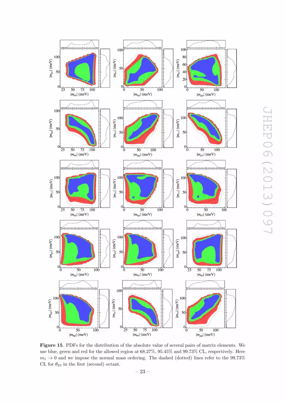
appendix B one can find the complete set of plots for this case (figure 15). We use the

same color coding as in previous figures. The range of the values allowed at 95.45% CL

are given in table 2.

– 7 –

JHEP06(2013)097

in meV

Element m1 = 0.1 eV

|mee| 39 – 108

|meµ| 11 – 88

|meτ | 11 – 78

|mµµ| 17 – 113

|mµτ | 21 – 111

|mττ | 31 – 113

Table 2. Range of allowed values of |mαβ | at 95.45 % CL for the quasi-degenerate case with

m1 = 0.1 eV.

Figure 5. Same as figure 3 but for m1 = 0.1 eV.

The correlations here are either similar to the very hierarchical case in normal ordering

or in the inverted ordering. For example, the PDFs for |mee|×|meµ|, |mµµ|×|mττ |, |mµµ|×|meτ | and |meµ| × |meτ |, are correlated like in the inverted ordering, while |mµτ | × |mττ |and |mee| × |mµτ | are more like the normal ordering.

3.1.3 Future perspectives

To evaluate the effect of a future determination of the mixing parameters on our knowl-

edge of the mass matrix we have studied the effect of reducing the uncertainty of each

parameter at a time while keeping the other parameters at their current uncertainties.

We assume that the following uncertainties will be achieved by the present or next gen-

eration experiments, at 68% CL. Accelerators experiments like for example T2K will be

able to measure δ(sin2 2θ23) ≈ 0.01 [6]. Possible medium baseline reactor experiments

– 8 –

JHEP06(2013)097

could, in principle, determine δ(∆m231) ≈ 7 × 10−6 eV2, δ(∆m2

21) ≈ 3 × 10−7 eV2, and

δ(sin2 θ12) ≈ 0.004 [7]. Within the current systematic uncertainties, the Daya Bay experi-

ment can probe δ(sin2 θ13) ≈ 0.0013 [2].

In figure 6 we illustrate the effect of a better determination of sin2 θ13 (top left panel),

∆m231 (top right panel), sin2 θ21 (bottom left panel) and sin2 θ23 (bottom right panel).

We observe that the effect of a better determination of any of these parameters is very

small. We have verified that this is true for both mass hierarchies and θ23 octants. The

biggest effect comes from a better determination of sin2 θ23, as one could have guessed, but

still this only reduces significantly the 3 σ region. We do not show the effect of a better

determination of ∆m221 because it is even smaller than for the other parameters.

On the other hand, a measurement of δ with an uncertainty of 10◦, that can be

envisaged according to ref. [38] for long baseline neutrino oscillation experiments, could be

significant. To illustrate this we show in figures 7–8 the effect of a determination of δ with

an uncertainty of 10◦ for some of the correlations between pairs of mass matrix elements.

On the top (bottom) panels of figure 7 we can see this for |mee| × |meµ| (|mµµ| × |meτ |)in the normal ordering for δ = 0◦ (left), 180◦ (center) and 270◦ (right), while on the top

(bottom) panels of figure 8 we show |mµτ | × |mττ | (|mµµ| × |meτ |) in the inverted ordering

for δ = 0◦ (left), 90◦ (center) and 180◦ (right), These cases for normal (inverted) ordering

and δ = 90◦ (δ = 270◦) are not shown because they are very similar to δ = 270◦ (δ = 90◦).

For the normal ordering, with m1 → 0, the determination of δ will play an important

role in the correlation of |mee| with all other mass matrix elements, but will be more

significant for |meµ| or |meτ |. This is due to the fact that for these mass matrix elements

the leading phase term is the one that accompanies cos [2(δ + λ3)], just as for |mee|. This

will also affect the correlations involving |mµµ| and |mττ |, since for them the leading phase

terms are, in order of importance, the ones that go with cos(2λ3) and cos(δ+2λ3). However,

the correlations with |mµτ | will only slightly change because the leading phase term for

this element does not depend on δ.

For the inverted ordering, with m3 → 0, the determination of δ will play a bigger role

in the PDFs of |mττ | and |mµµ|. This is because, as we can see from their expressions in

appendix A, the leading coefficients of cos(2λ1), cos(δ ± 2λ1) and cos δ are all of the same

order. The PDFs of |meµ| and |meτ | will also be affected because the terms that depend on

δ are not negligible in comparison to the leading term that depends on cos(2λ1), however

their relative importance will depend on the θ23 octant. The PDFs for |mee| and |mµτ | are

basically independent of δ, the first because m3 → 0, the second because these terms are

suppressed by sin2 θ13 or factors of this order.

We also have checked that the effect of the determination of δ for the quasi-degenerate

case with m1 = 0.1 eV is smaller than for the hierarchical cases because there are more

phases involved.

In the future we also expect to have information from three different sources: neutri-

noless double beta decay experiments, beta decay experiments and cosmology. In figure 9

we show the current allowed region for |mee| as a function of the effective electron neutrino

– 9 –

JHEP06(2013)097

mass, mβ and of the sum of the neutrino masses,1∑mi at 99% CL. The region allowed

by the normal (inverted) mass ordering is in blue (red) and the recent limit on |mee| given

by KamLAND-Zen [39], |mee| < (120 − 250) meV, is shown in gray. Cosmology excludes

the magenta region∑mi > (0.2− 0.6) eV [41]. Notice that the allowed regions were built

from the pdfs constructed from data (except for the CP phases, which we assumed to be

flat distributed). This is why the mee → 0 region is absent, as it is very unlikely to have

the necessary degree of cancellations.

The forecast sensitivity on |mee| of the most ambitious neutrinoless double beta decay

experiments, after 5 years of exposure, is 29-73 meV (GERDA phase-3) and 18-39 meV

(CUORE) [40].

The KArlsruhe TRitium Neutrino mass experiment (KATRIN) will have a sensitivity

on the electron neutrino effective mass, mβ =√∑

i |Uei|2m2i , of 0.2 eV at 95% CL [42].

Cosmological limits today still allow for quasi-degenerate neutrino masses; however,

this possibility will soon be confirmed or ruled out. According to ref. [41], many cosmo-

logical probes, with different systematics, will reach a sensitivity on∑mi of 0.1 eV or

lower. Lyman α forest can reach 0.1 eV, lensing of Cosmic Microwave Background 0.2-

0.05 eV, lensing of galaxies 0.07 eV, observations of the redshifted 21 cm neutral hydrogen

line 0.1-0.006 eV, galaxy clusters and galaxy distribution surveys 0.1 eV.

If cosmology will point to a quasi-degenerate neutrino spectrum:

1. the determination of δ by future experiments will not modify much the current cor-

relation among mass matrix elements;

2. |mee| should be in the reach of most proposed neutrinoless double beta decay exper-

iments, if neutrinos are of Majorana nature, ergo the non-observability of the 0νββ

would point to Dirac neutrinos;

3. mβ may be in the reach of KATRIN;

4. the ordering of neutrino masses can be settled by future neutrino oscillation experi-

ments but will not have great impact on the neutrino mass matrix;

5. if |mee| is measured we will also be able to constrain much more |meµ| and |meτ |.However, it will be very difficult to say something about the Majorana-CP phases.

On the other hand, cosmology can also place a limit on∑mi, such that we will know

if we have normal ordering with m1 → 0. In this case:

1. |mee| will be out of the reach of the proposed 0νββ experiments;

2. mβ will be out of the reach of KATRIN;

3. the experimental determination of δ will increase the correlation among mass matrix

elements and help to determine the structure of the neutrino mass matrix;

1There is no one-to-one correspondence between mee and mβ or∑imi. Hence, in order to plot figure 9,

for each value of m0 we extracted the allowed interval of mee and plotted it against mβ and∑imi calculated

at the best fit values of the oscillation parameters (as the Majorana phases do not play a role in these last

two quantities).

– 10 –

JHEP06(2013)097

4. the ordering of neutrino masses should be confirmed by future neutrino oscillation

experiments.

It may be the case that cosmology will rule out a quasi-degenerate spectrum, but not

the inverted ordering. If this happens:

1. |mee| may be in the reach of the proposed 0νββ experiments;

2. mβ will be out of the reach of KATRIN;

3. the ordering of neutrino masses should be determined by future neutrino oscillation

experiments;

4. the experimental determination of δ will increase the correlation among mass matrix

elements and help to determine the structure of the neutrino mass matrix, specially

if the mass ordering is known;

5. we may be able to say something about one of the Majorana CP phases, if |mee| is

measured.

These future advances may thus provide new clues for the understanding of the flavor

problem in the lepton sector. Some models of neutrino mixing based on discrete flavor

groups have predictions that can be tested in the future. For instance, the Lin model [33],

where the A4 symmetry is broken by additional Zn parities, predicts

sin2 θ23 =1

2+

1√2

sin θ13 cos δ.

Another example is the SUSY model based on the flavor symmetry group S4×Z4×U(1)

discussed in [34] where the relation

sin2 θ12 =1

2+ sin θ13 cos δ +O(sin2 θ13)

appears. Both relations can, in principle, be experimentally tested and, if true, they will

impose new correlations among the neutrino mass matrix elements.

Other models, such as the one presented in ref. [35], are even more predictive. This

model, which is based on a type-I seesaw framework with an underlying A4 flavor symmetry,

can, given a set of vacuum expectation value alignments for the flavon fields which break

the A4 symmetry, predict neutrino masses, the mass hierarchy, θ23 and δ.

There are also model-independent approaches to the flavor problem in the neutrino

sector. In ref. [36, 37], relations among the mixing parameters were obtained, in the

context of discrete flavor symmetries, under general assumptions that the flavor symmetry

group is of the von Dyck type. Again these relations can, in principle, be experimentally

tested, and if ratified by experiment induce more correlations among the mixing matrix

entries.

– 11 –

JHEP06(2013)097

Figure 6. PDFs for the distribution of: |mee| × |meτ | for the the normal hierarchy with sin2 θ13uncertainty reduced (top left panel); |mµµ| × |mττ | for the the normal hierarchy with ∆m2

31 un-

certainty reduced (top right panel); |mee| × |mµµ| for the the quasi-degenerate case with sin2 θ12uncertainty reduced (bottom left panel) and |meµ|×|mµµ| for the the inverted hierarchy with sin2 θ23uncertainty reduced (bottom right panel). The colored areas are for the present uncertainties of

the oscillation parameters, whereas the back lines are for the assumed future reduced uncertainty

of one of the parameters (see text for details).

4 The 3+1 scenario

Whether or not one deems this to be a plausible scenario, we still believe it is important

to examine what are its consequences to the possible textures of the neutrino mass matrix.

In this case the mixing matrix can be parametrized as

U =

c12 c13 c14 s12 c13 c14 s13 c14e

−iδ s14−s12 c23 − c12s13s23 eiδ c12 c23 − s12s13s23 eiδ c13 s23 0

s12 s23 − c12s13c23 eiδ −c12 s23 − s12s13c23 eiδ c13 c23 0

−c12 c13 s14 −s12 c13 s14 −s13 s14e−iδ c14

, (4.1)

where we use the same notation as in eq. (3.1). This expression can be readily derived

from [44] once we identify θs ≡ θ14 and we assume ~n = (1, 0, 0), i.e. the sterile state mixes

only with the electron neutrino. With this assumptions, there are no extra Dirac CP

– 12 –

JHEP06(2013)097

Figure 7. PDFs for the distribution of: |mee| × |meµ| (top panels) and |mµµ| × |meτ | (bottom

panels) for the normal ordering. From left to right δ = 0◦, 180◦ and 270◦, assumed to be determined

within 10◦.

Figure 8. PDFs for the distribution of: |mµτ | × |mττ | (top panels) and |mµµ| × |meτ | (bottom

panels) for the inverted ordering. From left to right δ = 0◦, 90◦ and 180◦, assumed to be determined

within 10◦.

phases. Nevertheless, there is one extra Majorana phase, λ4. The expression of all the

squared matrix elements, in the limit c13 ∼ c14 → 1, can be found in appendix A.

– 13 –

JHEP06(2013)097

Figure 9. We show the current allowed regions for |mee| at 99% CL as a function of the effective

electron neutrino mass, mβ , on the left panel and as a function of the sum of the neutrino masses,∑mi, on the right panel. The region allowed by the normal (inverted) mass ordering is in blue

(red), the recent limit on |mee| given by KamLAND-Zen [39] in gray and the region excluded

by cosmology [41] in magenta. We also show the reach expected for the beta decay experiment

Katrin [42], as well as the ultimate reach aimed by the neutrinoless double beta decay experiments

GERDA and CUORE according to ref. [40].

For simplicity, we examine here two cases: (a) ∆m241 = 1.71 eV2 and sin2 θ14 = (0.8−

4.2)× 10−2, (b) ∆m241 = 0.95 eV2 and sin2 θ14 = (0.8− 2.5)× 10−2, which are two possible

solutions to the reactor and gallium anomalies [23]. These solutions seem at first glance

to be at odds with cosmology, but we will ignore this fact at this point. Since sin2 θ14 is

small, we do not expect big changes in the PDFs of |mαβ|, α, β = e, µ, τ , except for the

case |mee|. We have explicitly checked that this is the case.

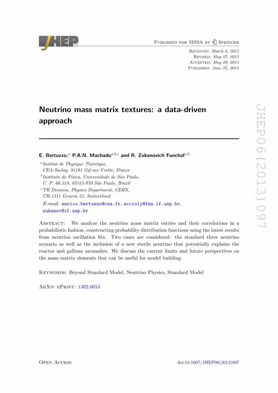
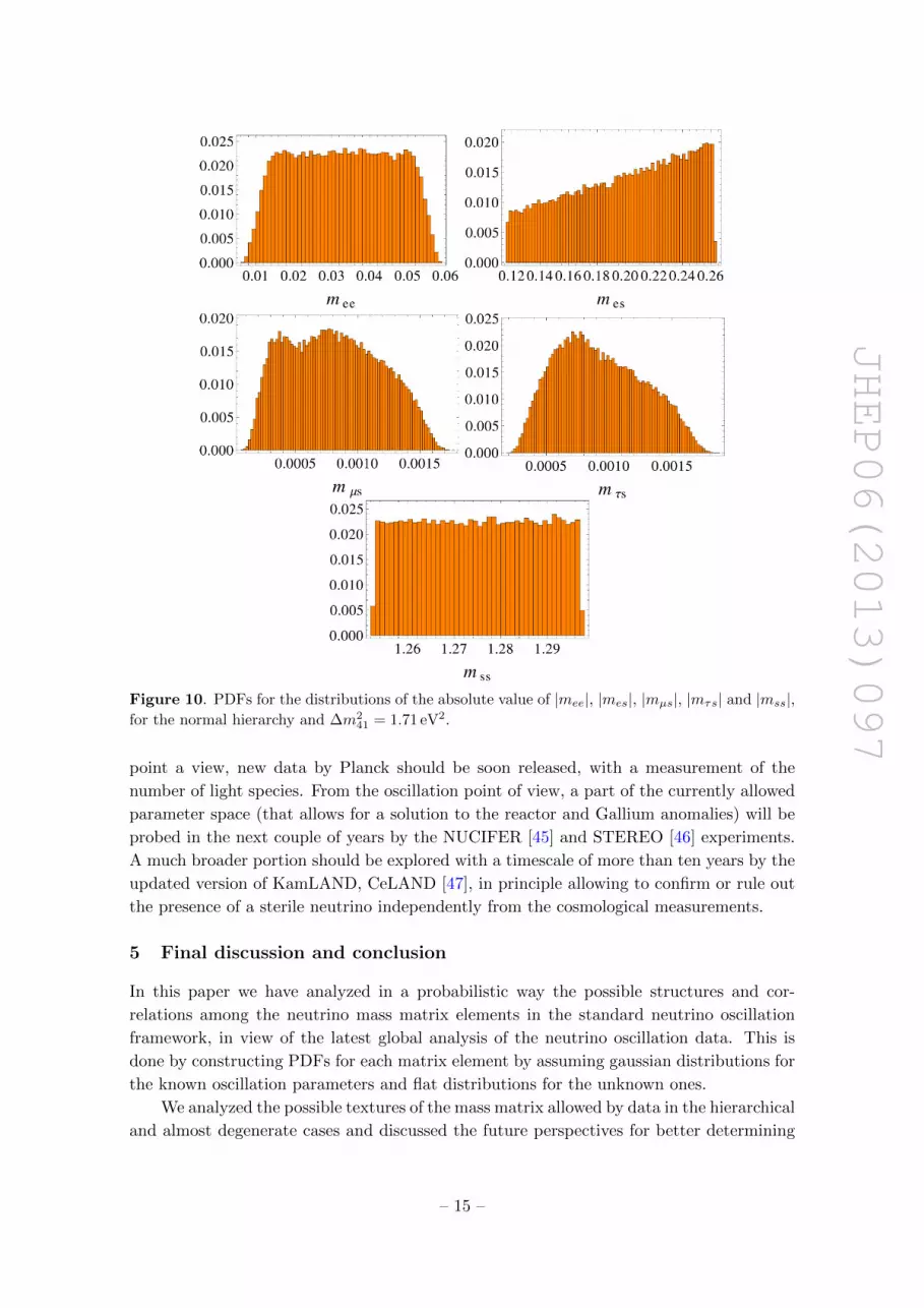
In figure 10 we show |mee| and the new entries |mαs|, α = e, µ, τ for the normal

hierarchy and ∆m241 = 1.71 eV2. For the case ∆m2

41 = 0.95 eV2, the plots would be similar

in shape, however with different scale. For |mee| the largest value goes down from 0.06 eV

to 0.045 eV. For |mes| the range changes from ∼(0.12 – 0.26) eV to ∼(0.09 – 0.20) eV. For

|mµs|, |mτs| there is basically no difference and for |mss| there is again a shift in the range

from ∼(1.25 – 1.30) eV to ∼(0.935 – 0.97) eV.

In figure 11 we show the correlations among the PDF’s of |mee| and |mes|, |mµs|, |mτs|,|mss|, for the normal hierarchy and ∆m2

41 = 1.71 eV2. Since the difference between the

case ∆m241 = 1.71 eV2 and ∆m2

41 = 0.95 eV2 is basically the scale, as commented above,

we do not show the correlations in this case either.

We observe that |mee| is very correlated with |mes|. This is easy to understand from

the formulae in appendix A, as |mee| goes as s214 while |mes| goes like s14 producing a

squared root behavior. The thickness is driven by the CP phases. The linear behavior

between |mee| and |mss| can be explained by noting that |mss| ≈ m4−|mee|. Again due to

the approximate µ-τ symmetry we get similar ranges and behaviors for |mee| × |mµs| and

|mee| × |mτs|.Also in this case it is interesting to consider future perspectives, in particular consid-

ering the interplay between oscillation experiments and cosmology. From the cosmology

– 14 –

JHEP06(2013)097

Figure 10. PDFs for the distributions of the absolute value of |mee|, |mes|, |mµs|, |mτs| and |mss|,for the normal hierarchy and ∆m2

41 = 1.71 eV2.

point a view, new data by Planck should be soon released, with a measurement of the

number of light species. From the oscillation point of view, a part of the currently allowed

parameter space (that allows for a solution to the reactor and Gallium anomalies) will be

probed in the next couple of years by the NUCIFER [45] and STEREO [46] experiments.

A much broader portion should be explored with a timescale of more than ten years by the

updated version of KamLAND, CeLAND [47], in principle allowing to confirm or rule out

the presence of a sterile neutrino independently from the cosmological measurements.

5 Final discussion and conclusion

In this paper we have analyzed in a probabilistic way the possible structures and cor-

relations among the neutrino mass matrix elements in the standard neutrino oscillation

framework, in view of the latest global analysis of the neutrino oscillation data. This is

done by constructing PDFs for each matrix element by assuming gaussian distributions for

the known oscillation parameters and flat distributions for the unknown ones.

We analyzed the possible textures of the mass matrix allowed by data in the hierarchical

and almost degenerate cases and discussed the future perspectives for better determining

– 15 –

JHEP06(2013)097

Figure 11. PDFs for the distributions of the absolute values |mee| × |mes|, |mee| × |mµs|, |mee| ×|mτs| and |mee| × |mss|, for the normal hierarchy and ∆m2

41 = 1.71 eV2.

these matrix elements by future neutrino oscillation and non-oscillation data. The conclu-

sion is that a better determination of the currently measured oscillation parameters will,

in general, have a small effect on the matrix elements. The biggest effect will come from a

better determination of sin2 θ23 solving the octant degeneracy, as one could have guessed.

A determination of δ would be significant, particularly for the normal hierarchy. In the

inverted ordering, it would play a bigger role in the determination of |mµτ | and |mττ |. For

the quasi-degenerate case, the impact of the determination of δ is rather small due to the

presence of more relevant CP phases. Future inputs from beta and neutrinoless double

beta decay experiments, as well as cosmology, seem to be the most promising in providing

new clues to understand the flavor structure. A specially encouraging scenario would be

to have mβ in the reach of KATRIN experiment, the neutrino mass hierarchy settled by

near future oscillation experiments, and also a possible cosmological measurement of the

sum of neutrino masses.

Models of neutrino mixing based on discrete flavor symmetries, as discussed at the

end of in section 3, anticipate relations among mixing angles and the δ phase that can be

tested in the future. If these relations turn out to be true, they will impose correlations

among the mass matrix elements beyond the ones considered here.

– 16 –

JHEP06(2013)097

Figure 12. We show the current allowed regions for |mee| at 99% CL as a function of the effective

electron neutrino mass, mβ , on the left panels and as a function of the sum of the neutrino masses,∑mi, on the right panels for the 3+1 scenario. Here ∆m2

41 = 1.71 eV2. The region allowed by the

normal (inverted) mass ordering is in blue (red), and the recent limit on |mee| given by KamLAND-

Zen [39] in gray. We also show the reach expected for the beta decay experiment Katrin [42], as

well as the ultimate reach aimed by the neutrinoless double beta decay experiments GERDA and

CUORE according to ref. [40].

We extend our analysis to include the possibility of a sterile neutrino with mass and

mixings allowed by the reactor and gallium anomalies (disregarding current cosmological

bounds). We discuss what are the modifications to the mass matrix pattern in this scenario,

finding only relevant modifications for mee as expected. Despite the presence of more

parameters than in the standard scenario, the larger sterile neutrino mass would make

easier to measure both |mee| and mβ. This may also have a big impact in cosmological

models, as well as in the future strategies for oscillation experiments.

Acknowledgments

This work was supported by Fundacao de Amparo a Pesquisa do Estado de Sao Paulo

(FAPESP), Conselho Nacional de Desenvolvimento Cientıfico e Tecnologico (CNPq), by

the European Commission under the contract PITN-GA-2009-237920 and by the Agence

National de la Recherche under contract ANR 2010 BLANC 0413 01. R.Z.F. acknowledges

partial support from the European Union FP7 ITN INVISIBLES (Marie Curie Actions,

PITN- GA-2011- 289442).

A Matrix elements squared

Here we give some approximate expressions for the matrix elements |mαβ|2. We use the

following notation: x2 = sin2 θ12, y2 = sin2 θ13, z

2 = sin2 θ23 and w2 = sin2 θ14. Here we

set√

1− y2 → 1 and√

1− w2 → 1. The standard case is recovered by taking w → 0.

|mee|2 ≈ m24w

4 +m22x

4 +m21

(1− x2

)2+m2

3y4

+2m1m4

(1− x2

)w2 cos [2 (λ1 − λ4)]

– 17 –

JHEP06(2013)097

+2m1m2 x2(1− x2

)cos (2λ1)

+2m1m3 y2(1− x2

)cos [2 (δ − λ1 + λ3)]

+2m2m4 x2w2 cos (2λ4)

+2m2m3 x2y2 cos [2 (δ + λ3)]

+2m3m4 y2w2 cos [2 (δ + λ3 − λ4)] (A.1)

|meµ|2 ≈(1− x2

)x2(1− z2)(m2

1 +m22) +

[m2

1

(1− x2

)2y2 +m2

2 x4y2 +m2

3 y2]z2

+[2m1m2 x

2y2z2(1− x2

)− 2m1m2 x

2(1− z2

) (1− x2

)]cos (2λ1)

−2m1m3 y2z2(1− x2) cos [2 (δ − λ1 + λ3)]

+[2m2

1 xyz(1− x2

)3/2√1− z2 − 2m2

2 x3yz√

1− x2√

1− z2]

cos δ

−2m1m2 xyz(1− x2

)3/2√1− z2 cos (δ − 2λ1)

−2m2m3 x2y2z2 cos [2 (δ + λ3)]

+2m2m3 xyz√

1− x2√

1− z2 cos (δ + 2λ3)

−2m1m3 xyz√

1− x2√

1− z2 cos (δ − 2λ1 + 2λ3)

+2m1m2 x3yz√

1− x2√

1− z2 cos (δ + 2λ1) (A.2)

|meτ |2 ≈(1− x2

)x2z2(m2

1 +m22) +

[m2

1

(1− x2

)2y2 +m2

2 x4y2 +m2

3 y2]

(1− z2)

+[2m1m2 x

2y2(1− z2)(1− x2

)− 2m1m2 x

2z2(1− x2

)]cos (2λ1)

−2m1m3 y2(1− z2)(1− x2) cos [2 (δ − λ1 + λ3)]

−[2m2

1 xyz(1− x2

)3/2√1− z2 − 2m2

2 x3yz√

1− x2√

1− z2]

cos δ

+2m1m2 xyz(1− x2

)3/2√1− z2 cos (δ − 2λ1)

−2m2m3 x2y2(1− z2) cos [2 (δ + λ3)]

−2m2m3 xyz√

1− x2√

1− z2 cos (δ + 2λ3)

+2m1m3 xyz√

1− x2√

1− z2 cos (δ − 2λ1 + 2λ3)

−2m1m2 x3yz√

1− x2√

1− z2 cos (δ + 2λ1) (A.3)

|mµµ|2 ≈ 4(1− z2

)x2y2z2(1− x2)(m2

1 +m22) + (1− z2)2

[m2

1x4 +m2

2(1− x2)2]

+[m2

1

(1− x2

)2y4 +m2

2 x4y4 +m2

3

]z4

+2m1m2 x2(1− x2

) [(1− z2)2 − 4 y2z2

(1− z2

)+ y4z4

]cos (2λ1)

+2m1m2 (1− z2)x4y2z2 cos [2 (δ + λ1)]

+2m1m2 (1− z2)(1− x)2(1 + x)2y2z2 cos [2 (δ − λ1)]+2m2m3 (1− z2)(1− x2)z2 cos (2λ3)

+2 (m21 +m2

2) (1− z2)(1− x2)x2y2z2 cos (2δ)

+4m1m3

√1− z2

√1− x2xyz3 cos (δ − 2λ1 + 2λ3)

−4m2m3

√1− z2

√1− x2xyz3 cos (δ + 2λ3)

+4m1m2 x3yz√

1− z2√

1− x2[y2z2 − (1− z2)

]cos (δ + 2λ1)

−4xyz√

1− x2√

1− z2[m2

1

(x2((y2 + 1

)z2 − 1

)− y2z2

)

– 18 –

JHEP06(2013)097

+ m22

(x2((y2 + 1

)z2 − 1

)− z2 + 1

)]cos (δ)

+4m1m2 xyz√

1− z2√

1− x2 (1− x2)[1− (1 + y2)z2

]cos (δ − 2λ1)

+2m2m3 x2y2z4 cos [2 (δ + λ3)]

+2m1m3 (1− x2)y2z4 cos [2 (δ − λ1 + λ3)]

+2m1m3 (1− z2)x2z2 cos [2 (λ1 − λ3)] (A.4)

|mµτ |2 ≈ (1− z2)z2[m2

3 + (1− x2)2(m21 y

4 +m22) + x4(m2

1 +m22 y

4)]

+(1− x2)x2y2 (m21 +m2

2)[(1− z2)2 + z4

]+2m1m2 x

2[z2(1− z2)((1 + y2)2 − x2)− y2(1− x2)(z4 + (1− z2)2)

]cos (2λ1)

+2xyz(1− 2z2)√

1− z2√

1− x2[(1− x2)(m2

2 +m21y

2)− x2(m21 +m2

2y2)]

cos δ

−2m1m2 xyz(1− 2z2)√

1− z2(1− x2)3/2(1 + y2) cos (δ − 2λ1)

+2m1m3 xyz(1− 2z2)√

1− z2√

1− x2 cos (δ − 2λ1 + 2λ3)

−2m2m3 xyz(1− 2z2)√

1− z2√

1− x2 cos (δ + 2λ3)

−2 (m21 +m2

2) (1− z2)(1− x2)x2y2z2 cos (2δ)

−2m2m3 (1− z2)(1− x2)z2 cos (2λ3)

+2m1m2 x3yz(1− 2z2)

√1− z2

√1− x2(1 + y2) cos (δ + 2λ1)

−2m1m2 y2z2(1− z2)(1− x2)2 cos [2 (δ − λ1)]

−2m1m2 x4y2z2(1− z2) cos [2 (δ + λ1)]

+2m2m3 x2y2z2(1− z2) cos [2 (δ + λ3)]

+m1m3 y2(1− x2) cos [2 (δ − λ1 + λ3)]

−2m1m3 (1− z2)x2z2 cos [2 (λ1 − λ3)] (A.5)

|mττ |2 ≈ 4(1− z2

)x2y2z2(1− x2)(m2

1 +m22) + z4

[m2

1x4 +m2

2(1− x2)2]

+[m2

1

(1− x2

)2y4 +m2

2 x4y4 +m2

3

](1− z2)2

+2m1m2 x2(1− x2

) [y4(1− z2)2 − 4 y2z2

(1− z2

)+ z4

]cos (2λ1)

+2m1m2 (1− z2)x4y2z2 cos [2 (δ + λ1)]

+2m1m2 (1− z2)(1− x)2(1 + x)2y2z2 cos [2 (δ − λ1)]+2m2m3 (1− z2)(1− x2)z2 cos (2λ3)

+2 (m21 +m2

2) (1− z2)(1− x2)x2y2z2 cos (2δ)

−4m1m3

√1− z2

√1− x2xyz(1− z2) cos (δ − 2λ1 + 2λ3)

+4m2m3

√1− z2

√1− x2xyz(1− z2) cos (δ + 2λ3)

+4m1m2 x3yz√

1− z2√

1− x2[y2z2 − y2 + z2

]cos (δ + 2λ1)

−4xyz√

1− x2√

1− z2[m2

1

((1− x2

)y2(1− z2

)+ x2z2

)− m2

2

(x2y2

(1− z2

)+ z2(1− x2)

)]cos (δ)

+4m1m2 xyz√

1− z2√

1− x2 (1− x2)[(1− z2)y2 − z2

]cos (δ − 2λ1)

+2m2m3 x2y2(1− z)2(1 + z)2 cos [2 (δ + λ3)]

+2m1m3 (1− x2)y2(1− z)2(1 + z)2 cos [2 (δ − λ1 + λ3)]

– 19 –

JHEP06(2013)097

+2m1m3 (1− z2)x2z2 cos [2 (λ1 − λ3)] (A.6)

|mse|2 ≈ w2[m2

2x4 +m2

1

(1− x2

)2+m2

3y4 +m2

4

]−2m3m4w

2y2 cos [2 (δ + λ3 − λ4)]+2m1m2w

2x2(1− x2

)cos (2λ1)

+2m1m3w2y2(1− x2

)cos [2 (δ − λ1 + λ3)]

−2m1m4w2(1− x2

)cos [2 (λ1 − λ4)]

+2m2m3w2x2y2 cos [2 (δ + λ3)]

−2m2m4w2x2 cos (2λ4) (A.7)

|msµ|2 ≈ w2[m2

1

(x2 − 1

) (x2((y2 + 1

)z2 − 1

)− y2z2

)+m2

2x2(x2((y2 + 1

)z2 − 1

)− z2 + 1

)+m2

3y2z2]

+2w2xyz√

1− x2√

1− z2[(1− x2)m2

1 − x2m22

]cos δ

−2m1m2w2xyz(1− x2)3/2

√1− z2 cos (δ − 2λ1)

+2m1m2w2x3yz

√1− x2

√1− z2 cos (δ + 2λ1)

−2m1m3w2xyz

√1− x2

√1− z2 cos (δ − 2λ1 + 2λ3)

+2m2m3w2xyz

√1− x2

√1− z2 cos (δ + 2λ3)

−2m2m3w2x2y2z2 cos [2 (δ + λ3)]

+2m1m2w2x2(1− x2)

[(1 + y2)z2 − 1

]cos (2λ1)

−2m1m3 (1− x2)w2y2z2 cos [2 (δ − λ1 + λ3)] (A.8)

|msτ |2 ≈ w2[m2

1

(1− x2

) ((1− x2

)y2(1− z2

)+ x2z2

)+ m2

2

(x2z2 + x4

(y2(1− z2

)− z2

))+m2

3y2(1− z2

)]−2w2xyz

√1− x2

√1− z2

[(1− x2)m2

1 − x2m22

]cos δ

+2m1m2w2xyz(1− x2)3/2

√1− z2 cos (δ − 2λ1)

−2m1m2w2x3yz

√1− x2

√1− z2 cos (δ + 2λ1)

+2m1m3w2xyz

√1− x2

√1− z2 cos (δ − 2λ1 + 2λ3)

−2m2m3w2xyz

√1− x2

√1− z2 cos (δ + 2λ3)

−2m2m3w2x2y2(1− z2) cos [2 (δ + λ3)]

−2m1m2w2x2(1− x2)

[z2 − (1− z2)y2

]cos (2λ1)

−2m1m3 (1− x2)w2y2(1− z2) cos [2 (δ − λ1 + λ3)] (A.9)

|mss|2 ≈ w4[(1− x2)2m2

1 + x4m22 + y4m2

3

]+m2

4

+2m1m2w4x2(1− x2) cos(2λ1)

+2m2m4w4x2 cos(2λ4)

+2m1m3w4y2(1− x2) cos [2 (δ − λ1 + λ3)]

+2m1m4w2(1− x2) cos [2 (λ1 − λ4)]

+2m2m3w4x2y2 cos [2 (δ + λ3)]

+2m3m4w2y2 cos [2 (δ + λ3 − λ4)] (A.10)

– 20 –

JHEP06(2013)097

B Complete set of correlation plots for the matrix elements

Figure 13. PDFs for the distribution of the absolute value of several pairs of matrix elements.

We use blue, green and red for the allowed region at 68.27%, 95.45% and 99.73% CL, respectively.

Here m1 → 0. The dashed (dotted) lines refer to the 99.73% CL for θ23 in the first (second) octant.

– 21 –

JHEP06(2013)097

Figure 14. PDFs for the distribution of the absolute value of several pairs of matrix elements.

We use blue, green and red for the allowed region at 68.27%, 95.45% and 99.73% CL, respectively.

Here m3 → 0. The dashed (dotted) lines refer to the 99.73% CL for θ23 in the first (second) octant.

– 22 –

JHEP06(2013)097

Figure 15. PDFs for the distribution of the absolute value of several pairs of matrix elements. We

use blue, green and red for the allowed region at 68.27%, 95.45% and 99.73% CL, respectively. Here

m1 → 0 and we impose the normal mass ordering. The dashed (dotted) lines refer to the 99.73%

CL for θ23 in the first (second) octant.

– 23 –

JHEP06(2013)097

Open Access. This article is distributed under the terms of the Creative Commons

Attribution License which permits any use, distribution and reproduction in any medium,

provided the original author(s) and source are credited.

References

[1] DOUBLE-CHOOZ collaboration, Y. Abe et al., Indication for the disappearance of reactor

electron antineutrinos in the Double CHOOZ experiment, Phys. Rev. Lett. 108 (2012) 131801

[arXiv:1112.6353] [INSPIRE].

[2] DAYA-BAY collaboration, F. An et al., Observation of electron-antineutrino disappearance

at Daya Bay, Phys. Rev. Lett. 108 (2012) 171803 [arXiv:1203.1669] [INSPIRE].

[3] RENO collaboration, J. Ahn et al., Observation of Reactor Electron Antineutrino

Disappearance in the RENO Experiment, Phys. Rev. Lett. 108 (2012) 191802

[arXiv:1204.0626] [INSPIRE].

[4] T2K collaboration, K. Abe et al., Indication of Electron Neutrino Appearance from an

Accelerator-produced Off-axis Muon Neutrino Beam, Phys. Rev. Lett. 107 (2011) 041801

[arXiv:1106.2822] [INSPIRE].

[5] MINOS collaboration, P. Adamson et al., Improved search for muon-neutrino to

electron-neutrino oscillations in MINOS, Phys. Rev. Lett. 107 (2011) 181802

[arXiv:1108.0015] [INSPIRE].

[6] S. Emery, T2K, in Rencontres IPhT/SPP, Paris, France, June 2013.

[7] Y. Takaesu, Determination of the mass hierarchy with medium-baseline reactor-neutrino

experiments, arXiv:1304.5306 [INSPIRE].

[8] P. Machado, H. Minakata, H. Nunokawa and R. Zukanovich Funchal, Combining Accelerator

and Reactor Measurements of θ13: The First Result, JHEP 05 (2012) 023

[arXiv:1111.3330] [INSPIRE].

[9] G. Fogli, E. Lisi, A. Marrone, D. Montanino, A. Palazzo et al., Global analysis of neutrino

masses, mixings and phases: entering the era of leptonic CP-violation searches, Phys. Rev. D

86 (2012) 013012 [arXiv:1205.5254] [INSPIRE].

[10] M. Gonzalez-Garcia, M. Maltoni, J. Salvado and T. Schwetz, Global fit to three neutrino

mixing: critical look at present precision, JHEP 12 (2012) 123 [arXiv:1209.3023] [INSPIRE].

[11] D. Forero, M. Tortola and J. Valle, Global status of neutrino oscillation parameters after

Neutrino-2012, Phys. Rev. D 86 (2012) 073012 [arXiv:1205.4018] [INSPIRE].

[12] LSND collaboration, C. Athanassopoulos et al., Evidence for νµ → νe oscillations from the

LSND experiment at LAMPF, Phys. Rev. Lett. 77 (1996) 3082 [nucl-ex/9605003] [INSPIRE].

[13] LSND collaboration, A. Aguilar-Arevalo et al., Evidence for neutrino oscillations from the

observation of anti-neutrino(electron) appearance in a anti-neutrino(muon) beam, Phys. Rev.

D 64 (2001) 112007 [hep-ex/0104049] [INSPIRE].

[14] MiniBooNE collaboration, A. Aguilar-Arevalo et al., Event Excess in the MiniBooNE Search

for νµ → νe Oscillations, Phys. Rev. Lett. 105 (2010) 181801 [arXiv:1007.1150] [INSPIRE].

[15] GALLEX collaboration, P. Anselmann et al., First results from the Cr-51 neutrino source

experiment with the GALLEX detector, Phys. Lett. B 342 (1995) 440 [INSPIRE].

– 24 –

JHEP06(2013)097

[16] GALLEX collaboration, W. Hampel et al., Final results of the Cr-51 neutrino source

experiments in GALLEX, Phys. Lett. B 420 (1998) 114 [INSPIRE].

[17] F. Kaether, W. Hampel, G. Heusser, J. Kiko and T. Kirsten, Reanalysis of the GALLEX

solar neutrino flux and source experiments, Phys. Lett. B 685 (2010) 47 [arXiv:1001.2731]

[INSPIRE].

[18] SAGE collaboration, J. Abdurashitov et al., Measurement of the response of the

Russian-American gallium experiment to neutrinos from a Cr-51 source, Phys. Rev. C 59

(1999) 2246 [hep-ph/9803418] [INSPIRE].

[19] J. Abdurashitov, V. Gavrin, S. Girin, V. Gorbachev, P. Gurkina et al., Measurement of the

response of a Ga solar neutrino experiment to neutrinos from an Ar-37 source, Phys. Rev. C

73 (2006) 045805 [nucl-ex/0512041] [INSPIRE].

[20] SAGE collaboration, J. Abdurashitov et al., Measurement of the solar neutrino capture rate

with gallium metal. III: Results for the 2002–2007 data-taking period, Phys. Rev. C 80

(2009) 015807 [arXiv:0901.2200] [INSPIRE].

[21] T. Mueller, D. Lhuillier, M. Fallot, A. Letourneau, S. Cormon et al., Improved Predictions of

Reactor Antineutrino Spectra, Phys. Rev. C 83 (2011) 054615 [arXiv:1101.2663] [INSPIRE].

[22] P. Huber, On the determination of anti-neutrino spectra from nuclear reactors, Phys. Rev. C

84 (2011) 024617 [Erratum ibid. C 85 (2012) 029901] [arXiv:1106.0687] [INSPIRE].

[23] G. Mention, M. Fechner, T. Lasserre, T. Mueller, D. Lhuillier et al., The Reactor

Antineutrino Anomaly, Phys. Rev. D 83 (2011) 073006 [arXiv:1101.2755] [INSPIRE].

[24] J. Kopp, M. Maltoni and T. Schwetz, Are there sterile neutrinos at the eV scale?, Phys. Rev.

Lett. 107 (2011) 091801 [arXiv:1103.4570] [INSPIRE].

[25] C. Giunti and M. Laveder, 3+1 and 3+2 Sterile Neutrino Fits, Phys. Rev. D 84 (2011)

073008 [arXiv:1107.1452] [INSPIRE].

[26] P. Machado, H. Nunokawa, F.P. dos Santos and R.Z. Funchal, Bulk Neutrinos as an

Alternative Cause of the Gallium and Reactor Anti-neutrino Anomalies, Phys. Rev. D 85

(2012) 073012 [arXiv:1107.2400] [INSPIRE].

[27] M. Frigerio and A.Y. Smirnov, Structure of neutrino mass matrix and CP-violation, Nucl.

Phys. B 640 (2002) 233 [hep-ph/0202247] [INSPIRE].

[28] M. Frigerio and A.Y. Smirnov, Neutrino mass matrix: Inverted hierarchy and CP-violation,

Phys. Rev. D 67 (2003) 013007 [hep-ph/0207366] [INSPIRE].

[29] A. Merle and W. Rodejohann, The Elements of the neutrino mass matrix: Allowed ranges

and implications of texture zeros, Phys. Rev. D 73 (2006) 073012 [hep-ph/0603111]

[INSPIRE].

[30] W. Grimus and P. Ludl, Correlations of the elements of the neutrino mass matrix, JHEP 12

(2012) 117 [arXiv:1209.2601] [INSPIRE].

[31] CHOOZ collaboration, M. Apollonio et al., Search for neutrino oscillations on a long

baseline at the CHOOZ nuclear power station, Eur. Phys. J. C 27 (2003) 331

[hep-ex/0301017] [INSPIRE].

[32] MINOS collaboration, P. Adamson et al., Measurement of the neutrino mass splitting and

flavor mixing by MINOS, Phys. Rev. Lett. 106 (2011) 181801 [arXiv:1103.0340] [INSPIRE].

– 25 –

JHEP06(2013)097

[33] Y. Lin, Tri-bimaximal Neutrino Mixing from A4 and θ13 ∼ θC , Nucl. Phys. B 824 (2010) 95

[arXiv:0905.3534] [INSPIRE].

[34] G. Altarelli, F. Feruglio, L. Merlo and E. Stamou, Discrete Flavour Groups, theta13 and

Lepton Flavour Violation, JHEP 08 (2012) 021 [arXiv:1205.4670] [INSPIRE].

[35] M.-C. Chen, J. Huang, J.-M. O’Bryan, A.M. Wijangco and F. Yu, Compatibility of θ13 and

the Type I Seesaw Model with A4 Symmetry, JHEP 02 (2013) 021 [arXiv:1210.6982]

[INSPIRE].

[36] D. Hernandez and A.Y. Smirnov, Lepton mixing and discrete symmetries, Phys. Rev. D 86

(2012) 053014 [arXiv:1204.0445] [INSPIRE].

[37] D. Hernandez and A.Y. Smirnov, Discrete symmetries and model-independent patterns of

lepton mixing, arXiv:1212.2149 [INSPIRE].

[38] P. Coloma, P. Huber, J. Kopp and W. Winter, Systematic uncertainties in long-baseline

neutrino oscillations for large θ13, arXiv:1209.5973 [INSPIRE].

[39] KamLAND-Zen collaboration, A. Gando et al., Limit on Neutrinoless ββ Decay of Xe-136

from the First Phase of KamLAND-Zen and Comparison with the Positive Claim in Ge-76,

Phys. Rev. Lett. 110 (2013) 062502 [arXiv:1211.3863] [INSPIRE].

[40] X. Sarazin, Review of double beta experiments, arXiv:1210.7666 [INSPIRE].

[41] K. Abazajian, E. Calabrese, A. Cooray, F. De Bernardis, S. Dodelson et al., Cosmological

and Astrophysical Neutrino Mass Measurements, Astropart. Phys. 35 (2011) 177

[arXiv:1103.5083] [INSPIRE].

[42] KATRIN collaboration, S. Fischer, Status of the KATRIN experiment,

PoS(EPS-HEP2011)097.

[43] A. Belesev, A. Berlev, E. Geraskin, A. Golubev, N. Likhovid et al., An upper limit on

additional neutrino mass eigenstate in 2 to 100 eV region from ‘Troitsk nu-mass’ data, JETP

Lett. 97 (2013) 67 [arXiv:1211.7193] [INSPIRE].

[44] M. Cirelli, G. Marandella, A. Strumia and F. Vissani, Probing oscillations into sterile

neutrinos with cosmology, astrophysics and experiments, Nucl. Phys. B 708 (2005) 215

[hep-ph/0403158] [INSPIRE].

[45] http://indico.cern.ch/getFile.py/access?contribId=6&sessionId=7&resId=

0&materialId=slides&confId=207406.

[46] http://indico.cern.ch/getFile.py/access?contribId=7&sessionId=7&resId=

0&materialId=slides&confId=207406.

[47] M. Cribier, M. Fechner, T. Lasserre, A. Letourneau, D. Lhuillier et al., A proposed search for

a fourth neutrino with a PBq antineutrino source, Phys. Rev. Lett. 107 (2011) 201801

[arXiv:1107.2335] [INSPIRE].

– 26 –