Vector Solid Textures

Lvdi Wang1,4

1Tsinghua UniversityKun Zhou2

2Zhejiang UniversityYizhou Yu3

3University of Illinois at Urbana-ChampaignBaining Guo1,4

4Microsoft Research Asia

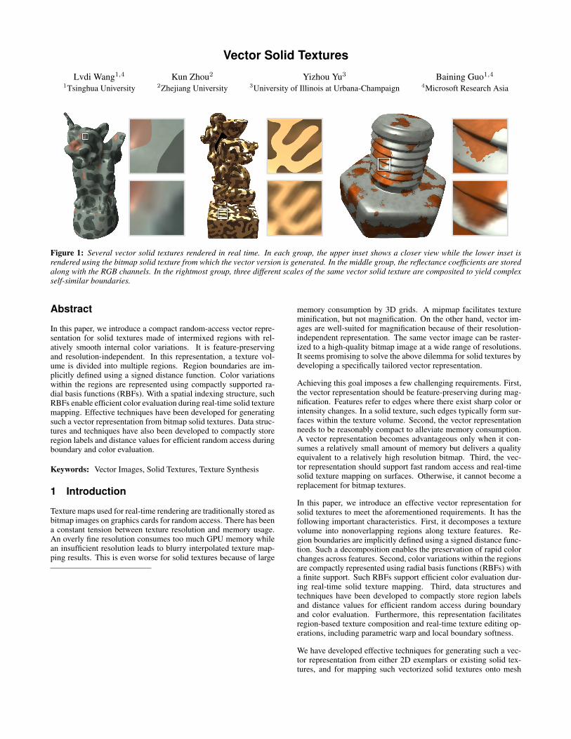
Figure 1: Several vector solid textures rendered in real time. In each group, the upper inset shows a closer view while the lower inset isrendered using the bitmap solid texture from which the vector version is generated. In the middle group, the reflectance coefficients are storedalong with the RGB channels. In the rightmost group, three different scales of the same vector solid texture are composited to yield complexself-similar boundaries.

Abstract

In this paper, we introduce a compact random-access vector repre-sentation for solid textures made of intermixed regions with rel-atively smooth internal color variations. It is feature-preservingand resolution-independent. In this representation, a texture vol-ume is divided into multiple regions. Region boundaries are im-plicitly defined using a signed distance function. Color variationswithin the regions are represented using compactly supported ra-dial basis functions (RBFs). With a spatial indexing structure, suchRBFs enable efficient color evaluation during real-time solid texturemapping. Effective techniques have been developed for generatingsuch a vector representation from bitmap solid textures. Data struc-tures and techniques have also been developed to compactly storeregion labels and distance values for efficient random access duringboundary and color evaluation.

Keywords: Vector Images, Solid Textures, Texture Synthesis

1 Introduction

Texture maps used for real-time rendering are traditionally stored asbitmap images on graphics cards for random access. There has beena constant tension between texture resolution and memory usage.An overly fine resolution consumes too much GPU memory whilean insufficient resolution leads to blurry interpolated texture map-ping results. This is even worse for solid textures because of large

memory consumption by 3D grids. A mipmap facilitates textureminification, but not magnification. On the other hand, vector im-ages are well-suited for magnification because of their resolution-independent representation. The same vector image can be raster-ized to a high-quality bitmap image at a wide range of resolutions.It seems promising to solve the above dilemma for solid textures bydeveloping a specifically tailored vector representation.

Achieving this goal imposes a few challenging requirements. First,the vector representation should be feature-preserving during mag-nification. Features refer to edges where there exist sharp color orintensity changes. In a solid texture, such edges typically form sur-faces within the texture volume. Second, the vector representationneeds to be reasonably compact to alleviate memory consumption.A vector representation becomes advantageous only when it con-sumes a relatively small amount of memory but delivers a qualityequivalent to a relatively high resolution bitmap. Third, the vec-tor representation should support fast random access and real-timesolid texture mapping on surfaces. Otherwise, it cannot become areplacement for bitmap textures.

In this paper, we introduce an effective vector representation forsolid textures to meet the aforementioned requirements. It has thefollowing important characteristics. First, it decomposes a texturevolume into nonoverlapping regions along texture features. Re-gion boundaries are implicitly defined using a signed distance func-tion. Such a decomposition enables the preservation of rapid colorchanges across features. Second, color variations within the regionsare compactly represented using radial basis functions (RBFs) witha finite support. Such RBFs support efficient color evaluation dur-ing real-time solid texture mapping. Third, data structures andtechniques have been developed to compactly store region labelsand distance values for efficient random access during boundaryand color evaluation. Furthermore, this representation facilitatesregion-based texture composition and real-time texture editing op-erations, including parametric warp and local boundary softness.

We have developed effective techniques for generating such a vec-tor representation from either 2D exemplars or existing solid tex-tures, and for mapping such vectorized solid textures onto mesh

surfaces in real time. During vectorization, color variations arefitted with a minimal number of RBFs using both nonlinear opti-mization and teleportation. The number of distinct region labels isminimized by casting it as a graph coloring problem. A spatial in-dexing structure is also set up for RBFs so that relevant RBFs canbe quickly looked up during real-time solid texture mapping.

Due to the use of signed distance functions and RBFs, our repre-sentation requires that the sharp features (region boundaries) in asolid texture can be identified by a binary mask and the regionshave relatively smooth internal color variations.

2 Related Work

Solid Texture Synthesis Solid textures are useful in many sce-narios, including modeling natural textures such as wood and mar-ble, and representing the interior or cross sections of volumetric ob-jects, such as fruits. Heeger and Bergen [1995] as well as Ghazan-farpour and Dischler [1995; 1996] did early work on example-basedsolid texture synthesis using parametric approaches. Wei attemptedto synthesize solid textures from 2D input using a non-parametricmethod [Efros and Leung 1999; Wei 2001]. Based on stereologi-cal techniques, Jagnow et al. [2004] generate impressive results foraggregate materials. But their method is not applicable for generalsolid textures. Qin and Yang [2007] propose an approach for gen-erating solid textures using aura matrices of the input exemplars.Kopf et al. [2007] present a widely applicable method that utilizes2D texture optimization [Kwatra et al. 2005] and histogram match-ing. We use their method to generate solid textures from 2D exem-plars. By considering the coherence within the 2D exemplars, Donget al. [2008] propose a parallel solid synthesis algorithm that runsefficiently on the GPU. Finally, Takayama et al. [2008] develop anintuitive interface that allows the user to design anisotropic solidtextures directly on objects using 3D exemplars.

In addition to texture synthesis, procedural textures (e.g. [Ebertet al. 1994; Worley 1996]) provide a practical alternative for solidtexture generation. Such textures typically do not save explicitcopies, but evaluate pointwise texture colors on the fly. Althoughimpressive visual results have been achieved on certain types of tex-tures, in general, it is still challenging to conceive a procedure thatconvincingly reproduces an arbitrarily chosen natural pattern. La-gae et al. [2009] introduce a procedural noise based on sparse Gaborconvolution that offers intuitive control over the spectral density,anisotropy etc. of the noise. But the variety of materials that can begenerated is still limited. Note that our vector texture representationrelies on the same tricubic interpolation as Perlin’s noise. However,we use it on signed distance values to determine region boundarieswhile Perlin used it for noise and gradient interpolation.

Vector Graphics and Image Vectorization 2D vector graphics,often in the form of charts, maps and clip arts, are curve-based andregions in-between curves are filled with uniform colors or colorgradients. Nehab and Hoppe [2008] introduced an algorithm forrandom-access rendering of antialiased 2D vector graphics on theGPU. It can map vector graphics onto arbitrary surfaces. There hasbeen much work on non-photographic image vectorization [Changand Hong 1998; Zou and Yan 2001; Hilaire and Tombre 2006],i.e. converting such an image into 2D vector graphics. These algo-rithms are mainly designed for contour tracing and curve fitting.

Vectorization of full-color 2D raster images [Lecot and Levy 2006;Price and Barrett 2006; Sun et al. 2007; Orzan et al. 2008; Laiet al. 2009; Xia et al. 2009] has been popular recently. These im-ages need a more generic vector representation that accounts forcolor variations across the image plane in addition to feature curves.Among them, high-quality image vectorization via a rectangulargrid of Ferguson patches has been explored in [Sun et al. 2007; Lai

et al. 2009]. Instead of using rectangular patches, Xia et al. [2009]exploits the topological flexibility of triangular patches with curvedboundaries to perform automatic feature alignment and image vec-torization. Diffusion curves [Orzan et al. 2008] model spatial colorvariations in a vectorized image as a diffusion from curves withboth color and blur attributes.

Several softwares, such as VectorEye, Vector Magic, and AutoTracehave been developed for automatically converting bitmaps to vectorgraphics. Commercial tools (CorelDRAW, Adobe Live Trace, etc.)that help artists design and edit vector images are also available.

In addition to complete vector representations, there exist hy-brid feature-based 2D texture representations (e.g. [Ramanarayananet al. 2004; Sen 2004; Tumblin and Choudhury 2004; Tarini andCignoni 2005; Parilov and Zorin 2008]). The basic idea of thesemethods is to improve the sharpness of the features in a magnifiedbitmap image by performing interpolation with respect to explicitlyadded feature boundaries. These methods represent features usingvector primitives but still represent spatial color variations using abitmap image. In comparison, our method works for 3D solid tex-tures where features are represented as implicit surfaces instead ofcurves. In addition, we represent color variations using compactlysupported RBFs, which are region-filling vector primitives moregeneric than uniform colors or color gradients.

3 Vector Texture RepresentationOur vector solid texture representation consists of three key com-ponents: a set of regions with distinct region labels, a continuous3D signed distance function, and the weights and parameters of aset of radial basis functions. The region boundaries are implicitlydefined by the zero isosurface of the signed distance function. Thisisosurface divides the texture volume into multiple connected com-ponents, and a region consists of one or multiple such connectedcomponents. The color variations within each region are repre-sented separately using a distinct subset of radial basis functions.

Both the signed distance function and region labels are definedthrough a 3D discrete grid, denoted as S, with d × d × d nodes.The sampled signed distance values and region labels at the gridnodes are explicitly stored. We denote xijk as the 3D location ofthe grid node (i, j, k), where i, j, k ∈ {0, 1, . . . , d−1}, andD(x),`(x) as the signed distance value and region label, respectively, atan arbitrary location x, which is not necessarily a grid node, insidethe texture volume. To define the underlying continuous signeddistance function, we calculate the signed distance at an arbitrarylocation by tricubic interpolation from the node values at the near-est 4× 4× 4 subgrid. Tricubic interpolation guarantees a sufficientlevel of continuity of the signed distance function.

The region label at an arbitrary location x is determined as follows.If all nodes in its nearest 2 × 2 × 2 subgrid have the same regionlabel, `(x) is assigned the same label too. Otherwise, there existsone or more boundary surfaces inside the subgrid, and the sign ofthe interpolated distance value at x determines `(x).

Note that representing region labels and the distance function us-ing a discrete grid is inherently different from representing colorson a grid. The former encodes feature-based texture segmentationresults as well as the shape of region boundaries. Such geometricinformation is essential for any vector representations, and plays acrucial role in feature preservation and magnification.

4 Vector Texture Generation

This section describes an algorithm to convert a bitmap solid textureto our vector representation.

Our algorithm requires a bitmap solid texture with an additionalchannel of signed distance as the input. Signed distance func-tions have been widely used as “feature maps” in texture synthe-sis [Lefebvre and Hoppe 2006; Kopf et al. 2007] to improve thesynthesis quality. This signed distance function is an implicit rep-resentation of texture features, i.e. surfaces that correspond to sharpedges in the texture volume.

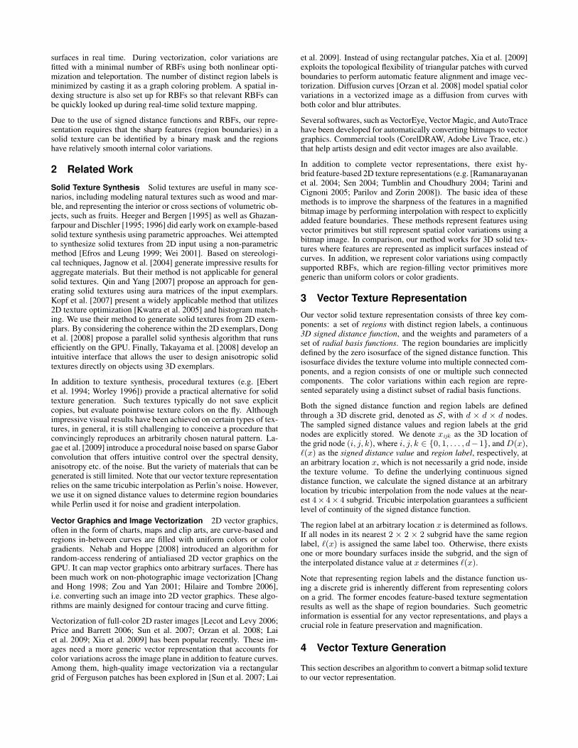
From 2D Exemplars Given an input 2D color texture and a bi-nary feature mask from which a 2D signed distance transformcan be computed, we adopt Kopf et al.’s optimization-based algo-rithm [2007] to synthesize a solid color texture with an additionalchannel of signed distance (Figure 2). The binary feature mask canbe created by color thresholding or user interaction.

C2D M2D D2D C3D D3D

Figure 2: Synthesizing the solid color texture C3D with signeddistance channel D3D (colorized according to the sign for clar-ity) from a 2D exemplar C2D and a signed distance transform D2D

computed from a binary feature mask M2D.

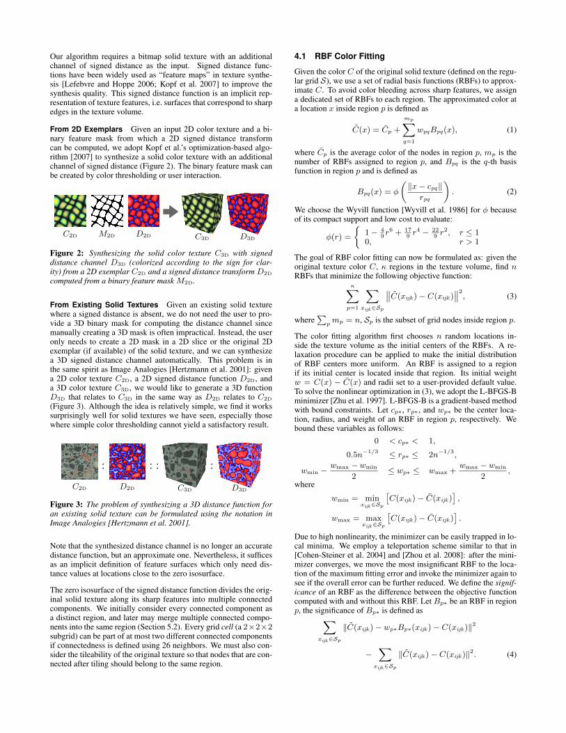
From Existing Solid Textures Given an existing solid texturewhere a signed distance is absent, we do not need the user to pro-vide a 3D binary mask for computing the distance channel sincemanually creating a 3D mask is often impractical. Instead, the useronly needs to create a 2D mask in a 2D slice or the original 2Dexemplar (if available) of the solid texture, and we can synthesizea 3D signed distance channel automatically. This problem is inthe same spirit as Image Analogies [Hertzmann et al. 2001]: givena 2D color texture C2D, a 2D signed distance function D2D, anda 3D color texture C3D, we would like to generate a 3D functionD3D that relates to C3D in the same way as D2D relates to C2D

(Figure 3). Although the idea is relatively simple, we find it workssurprisingly well for solid textures we have seen, especially thosewhere simple color thresholding cannot yield a satisfactory result.

C2D

:

D2D

: :

C3D

:

D3D

Figure 3: The problem of synthesizing a 3D distance function foran existing solid texture can be formulated using the notation inImage Analogies [Hertzmann et al. 2001].

Note that the synthesized distance channel is no longer an accuratedistance function, but an approximate one. Nevertheless, it sufficesas an implicit definition of feature surfaces which only need dis-tance values at locations close to the zero isosurface.

The zero isosurface of the signed distance function divides the orig-inal solid texture along its sharp features into multiple connectedcomponents. We initially consider every connected component asa distinct region, and later may merge multiple connected compo-nents into the same region (Section 5.2). Every grid cell (a 2×2×2subgrid) can be part of at most two different connected componentsif connectedness is defined using 26 neighbors. We must also con-sider the tileability of the original texture so that nodes that are con-nected after tiling should belong to the same region.

4.1 RBF Color Fitting

Given the color C of the original solid texture (defined on the regu-lar grid S), we use a set of radial basis functions (RBFs) to approx-imate C. To avoid color bleeding across sharp features, we assigna dedicated set of RBFs to each region. The approximated color ata location x inside region p is defined as

C(x) = Cp +

mp∑q=1

wpqBpq(x), (1)

where Cp is the average color of the nodes in region p, mp is thenumber of RBFs assigned to region p, and Bpq is the q-th basisfunction in region p and is defined as

Bpq(x) = φ

(‖x− cpq‖

rpq

). (2)

We choose the Wyvill function [Wyvill et al. 1986] for φ becauseof its compact support and low cost to evaluate:

φ(r) =

{1− 4

9r6 + 17

9r4 − 22

9r2, r ≤ 1

0, r > 1

The goal of RBF color fitting can now be formulated as: given theoriginal texture color C, κ regions in the texture volume, find nRBFs that minimize the following objective function:

κ∑p=1

∑xijk∈Sp

∥∥C(xijk )− C(xijk )∥∥2, (3)

where∑

pmp = n, Sp is the subset of grid nodes inside region p.

The color fitting algorithm first chooses n random locations in-side the texture volume as the initial centers of the RBFs. A re-laxation procedure can be applied to make the initial distributionof RBF centers more uniform. An RBF is assigned to a regionif its initial center is located inside that region. Its initial weightw = C(x) − C(x) and radii set to a user-provided default value.To solve the nonlinear optimization in (3), we adopt the L-BFGS-Bminimizer [Zhu et al. 1997]. L-BFGS-B is a gradient-based methodwith bound constraints. Let cp∗, rp∗, and wp∗ be the center loca-tion, radius, and weight of an RBF in region p, respectively. Webound these variables as follows:

0 < cp∗ < 1,

0.5n−1/3 ≤ rp∗ ≤ 2n−1/3,

wmin −wmax − wmin

2≤ wp∗ ≤ wmax +

wmax − wmin

2,

where

wmin = minxijk∈Sp

[C(xijk )− C(xijk )

],

wmax = maxxijk∈Sp

[C(xijk )− C(xijk )

].

Due to high nonlinearity, the minimizer can be easily trapped in lo-cal minima. We employ a teleportation scheme similar to that in[Cohen-Steiner et al. 2004] and [Zhou et al. 2008]: after the mini-mizer converges, we move the most insignificant RBF to the loca-tion of the maximum fitting error and invoke the minimizer again tosee if the overall error can be further reduced. We define the signif-icance of an RBF as the difference between the objective functioncomputed with and without this RBF. Let Bp∗ be an RBF in regionp, the significance of Bp∗ is defined as∑

xijk∈Sp

‖C(xijk )− wp∗Bp∗(xijk )− C(xijk )‖2

−∑

xijk∈Sp

‖C(xijk )− C(xijk )‖2. (4)

When teleporting an RBF to a new location that is inside a differentregion, the algorithm also dynamically changes the membership ofthe RBF to that region. The inclusion of this teleportation schemeleads to a further reduction of the objective function by 40%∼50%.

5 Compact StorageIn this section, we discuss a few effective techniques for reduc-ing the amount of memory required for storing the signed distancefunction and region labels.

5.1 Distance Quantization

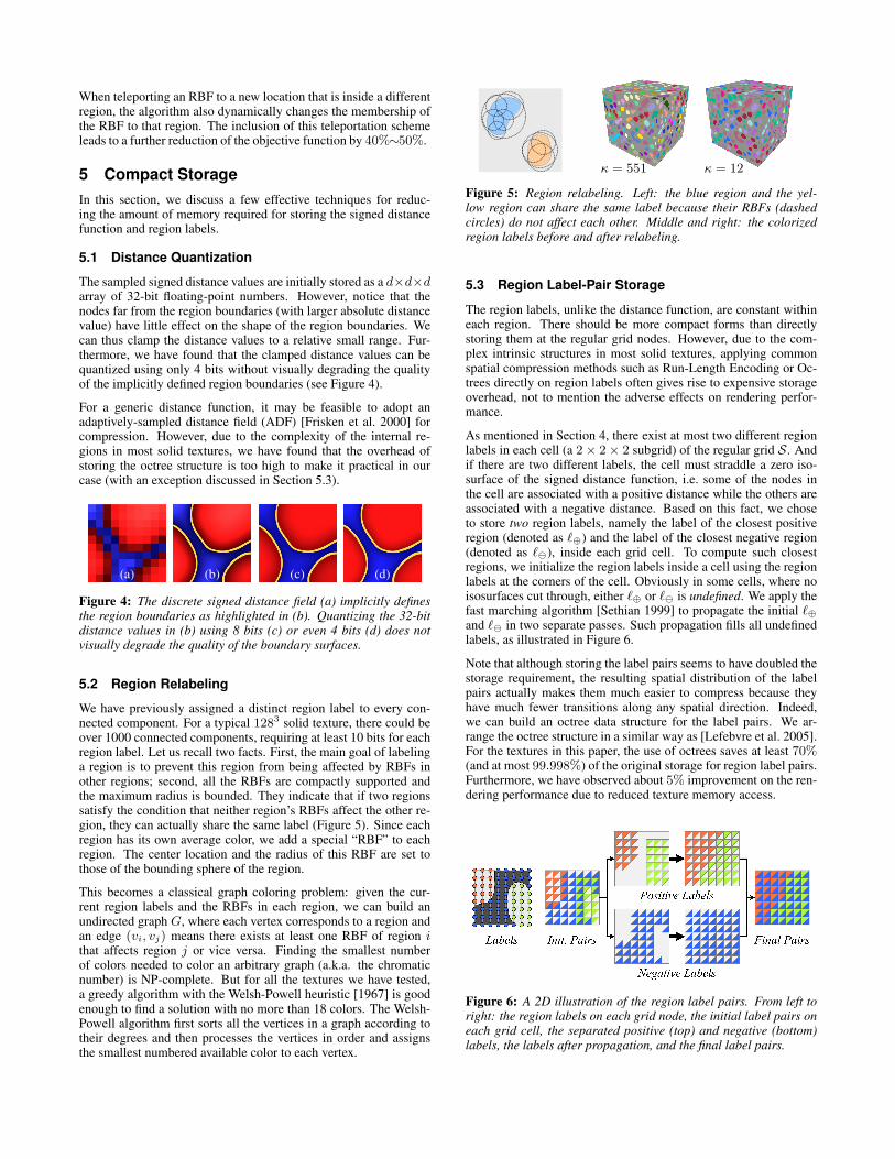
The sampled signed distance values are initially stored as a d×d×darray of 32-bit floating-point numbers. However, notice that thenodes far from the region boundaries (with larger absolute distancevalue) have little effect on the shape of the region boundaries. Wecan thus clamp the distance values to a relative small range. Fur-thermore, we have found that the clamped distance values can bequantized using only 4 bits without visually degrading the qualityof the implicitly defined region boundaries (see Figure 4).

For a generic distance function, it may be feasible to adopt anadaptively-sampled distance field (ADF) [Frisken et al. 2000] forcompression. However, due to the complexity of the internal re-gions in most solid textures, we have found that the overhead ofstoring the octree structure is too high to make it practical in ourcase (with an exception discussed in Section 5.3).

(a) (b) (c) (d)

Figure 4: The discrete signed distance field (a) implicitly definesthe region boundaries as highlighted in (b). Quantizing the 32-bitdistance values in (b) using 8 bits (c) or even 4 bits (d) does notvisually degrade the quality of the boundary surfaces.

5.2 Region Relabeling

We have previously assigned a distinct region label to every con-nected component. For a typical 1283 solid texture, there could beover 1000 connected components, requiring at least 10 bits for eachregion label. Let us recall two facts. First, the main goal of labelinga region is to prevent this region from being affected by RBFs inother regions; second, all the RBFs are compactly supported andthe maximum radius is bounded. They indicate that if two regionssatisfy the condition that neither region’s RBFs affect the other re-gion, they can actually share the same label (Figure 5). Since eachregion has its own average color, we add a special “RBF” to eachregion. The center location and the radius of this RBF are set tothose of the bounding sphere of the region.

This becomes a classical graph coloring problem: given the cur-rent region labels and the RBFs in each region, we can build anundirected graph G, where each vertex corresponds to a region andan edge (vi, vj) means there exists at least one RBF of region ithat affects region j or vice versa. Finding the smallest numberof colors needed to color an arbitrary graph (a.k.a. the chromaticnumber) is NP-complete. But for all the textures we have tested,a greedy algorithm with the Welsh-Powell heuristic [1967] is goodenough to find a solution with no more than 18 colors. The Welsh-Powell algorithm first sorts all the vertices in a graph according totheir degrees and then processes the vertices in order and assignsthe smallest numbered available color to each vertex.

κ = 551 κ = 12

Figure 5: Region relabeling. Left: the blue region and the yel-low region can share the same label because their RBFs (dashedcircles) do not affect each other. Middle and right: the colorizedregion labels before and after relabeling.

5.3 Region Label-Pair Storage

The region labels, unlike the distance function, are constant withineach region. There should be more compact forms than directlystoring them at the regular grid nodes. However, due to the com-plex intrinsic structures in most solid textures, applying commonspatial compression methods such as Run-Length Encoding or Oc-trees directly on region labels often gives rise to expensive storageoverhead, not to mention the adverse effects on rendering perfor-mance.

As mentioned in Section 4, there exist at most two different regionlabels in each cell (a 2× 2× 2 subgrid) of the regular grid S. Andif there are two different labels, the cell must straddle a zero iso-surface of the signed distance function, i.e. some of the nodes inthe cell are associated with a positive distance while the others areassociated with a negative distance. Based on this fact, we choseto store two region labels, namely the label of the closest positiveregion (denoted as `⊕) and the label of the closest negative region(denoted as `), inside each grid cell. To compute such closestregions, we initialize the region labels inside a cell using the regionlabels at the corners of the cell. Obviously in some cells, where noisosurfaces cut through, either `⊕ or ` is undefined. We apply thefast marching algorithm [Sethian 1999] to propagate the initial `⊕and ` in two separate passes. Such propagation fills all undefinedlabels, as illustrated in Figure 6.

Note that although storing the label pairs seems to have doubled thestorage requirement, the resulting spatial distribution of the labelpairs actually makes them much easier to compress because theyhave much fewer transitions along any spatial direction. Indeed,we can build an octree data structure for the label pairs. We ar-range the octree structure in a similar way as [Lefebvre et al. 2005].For the textures in this paper, the use of octrees saves at least 70%(and at most 99.998%) of the original storage for region label pairs.Furthermore, we have observed about 5% improvement on the ren-dering performance due to reduced texture memory access.

Figure 6: A 2D illustration of the region label pairs. From left toright: the region labels on each grid node, the initial label pairs oneach grid cell, the separated positive (top) and negative (bottom)labels, the labels after propagation, and the final label pairs.

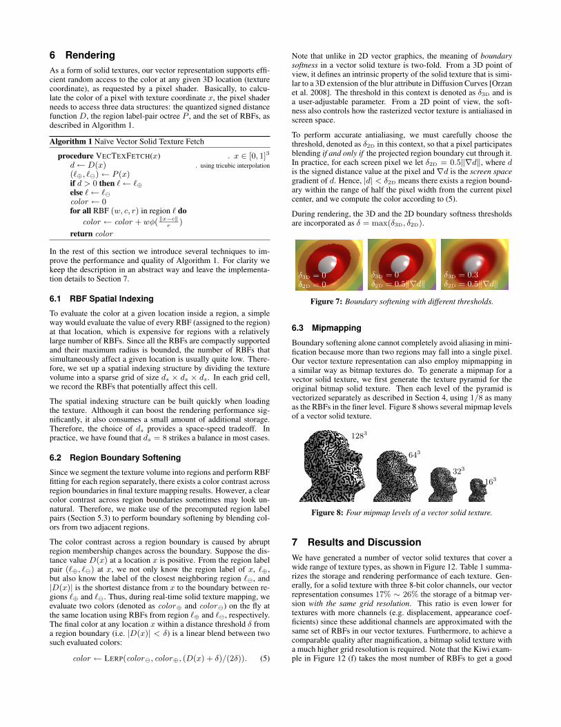
6 RenderingAs a form of solid textures, our vector representation supports effi-cient random access to the color at any given 3D location (texturecoordinate), as requested by a pixel shader. Basically, to calcu-late the color of a pixel with texture coordinate x, the pixel shaderneeds to access three data structures: the quantized signed distancefunction D, the region label-pair octree P , and the set of RBFs, asdescribed in Algorithm 1.

Algorithm 1 Naıve Vector Solid Texture Fetch

procedure VECTEXFETCH(x) . x ∈ [0, 1]3

d← D(x) . using tricubic interpolation(`⊕, `)← P (x)if d > 0 then `← `⊕else `← `color ← 0for all RBF (w, c, r) in region ` do

color ← color + wφ( ‖x−c‖r

)

return color

In the rest of this section we introduce several techniques to im-prove the performance and quality of Algorithm 1. For clarity wekeep the description in an abstract way and leave the implementa-tion details to Section 7.

6.1 RBF Spatial Indexing

To evaluate the color at a given location inside a region, a simpleway would evaluate the value of every RBF (assigned to the region)at that location, which is expensive for regions with a relativelylarge number of RBFs. Since all the RBFs are compactly supportedand their maximum radius is bounded, the number of RBFs thatsimultaneously affect a given location is usually quite low. There-fore, we set up a spatial indexing structure by dividing the texturevolume into a sparse grid of size ds × ds × ds. In each grid cell,we record the RBFs that potentially affect this cell.

The spatial indexing structure can be built quickly when loadingthe texture. Although it can boost the rendering performance sig-nificantly, it also consumes a small amount of additional storage.Therefore, the choice of ds provides a space-speed tradeoff. Inpractice, we have found that ds = 8 strikes a balance in most cases.

6.2 Region Boundary Softening

Since we segment the texture volume into regions and perform RBFfitting for each region separately, there exists a color contrast acrossregion boundaries in final texture mapping results. However, a clearcolor contrast across region boundaries sometimes may look un-natural. Therefore, we make use of the precomputed region labelpairs (Section 5.3) to perform boundary softening by blending col-ors from two adjacent regions.

The color contrast across a region boundary is caused by abruptregion membership changes across the boundary. Suppose the dis-tance value D(x) at a location x is positive. From the region labelpair (`⊕, `) at x, we not only know the region label of x, `⊕,but also know the label of the closest neighboring region `, and|D(x)| is the shortest distance from x to the boundary between re-gions `⊕ and `. Thus, during real-time solid texture mapping, weevaluate two colors (denoted as color⊕ and color) on the fly atthe same location using RBFs from region `⊕ and `, respectively.The final color at any location x within a distance threshold δ froma region boundary (i.e. |D(x)| < δ) is a linear blend between twosuch evaluated colors:

color ← LERP(color, color⊕, (D(x) + δ)/(2δ)). (5)

Note that unlike in 2D vector graphics, the meaning of boundarysoftness in a vector solid texture is two-fold. From a 3D point ofview, it defines an intrinsic property of the solid texture that is simi-lar to a 3D extension of the blur attribute in Diffusion Curves [Orzanet al. 2008]. The threshold in this context is denoted as δ3D and isa user-adjustable parameter. From a 2D point of view, the soft-ness also controls how the rasterized vector texture is antialiased inscreen space.

To perform accurate antialiasing, we must carefully choose thethreshold, denoted as δ2D in this context, so that a pixel participatesblending if and only if the projected region boundary cut through it.In practice, for each screen pixel we let δ2D = 0.5‖∇d‖, where dis the signed distance value at the pixel and ∇d is the screen spacegradient of d. Hence, |d| < δ2D means there exists a region bound-ary within the range of half the pixel width from the current pixelcenter, and we compute the color according to (5).

During rendering, the 3D and the 2D boundary softness thresholdsare incorporated as δ = max(δ3D, δ2D).

δ3D = 0δ2D = 0

δ3D = 0δ2D = 0.5‖∇d‖

δ3D = 0.3δ2D = 0.5‖∇d‖

Figure 7: Boundary softening with different thresholds.

6.3 Mipmapping

Boundary softening alone cannot completely avoid aliasing in mini-fication because more than two regions may fall into a single pixel.Our vector texture representation can also employ mipmapping ina similar way as bitmap textures do. To generate a mipmap for avector solid texture, we first generate the texture pyramid for theoriginal bitmap solid texture. Then each level of the pyramid isvectorized separately as described in Section 4, using 1/8 as manyas the RBFs in the finer level. Figure 8 shows several mipmap levelsof a vector solid texture.

1283

643

323

163

Figure 8: Four mipmap levels of a vector solid texture.

7 Results and DiscussionWe have generated a number of vector solid textures that cover awide range of texture types, as shown in Figure 12. Table 1 summa-rizes the storage and rendering performance of each texture. Gen-erally, for a solid texture with three 8-bit color channels, our vectorrepresentation consumes 17% ∼ 26% the storage of a bitmap ver-sion with the same grid resolution. This ratio is even lower fortextures with more channels (e.g. displacement, appearance coef-ficients) since these additional channels are approximated with thesame set of RBFs in our vector textures. Furthermore, to achieve acomparable quality after magnification, a bitmap solid texture witha much higher grid resolution is required. Note that the Kiwi exam-ple in Figure 12 (f) takes the most number of RBFs to get a good

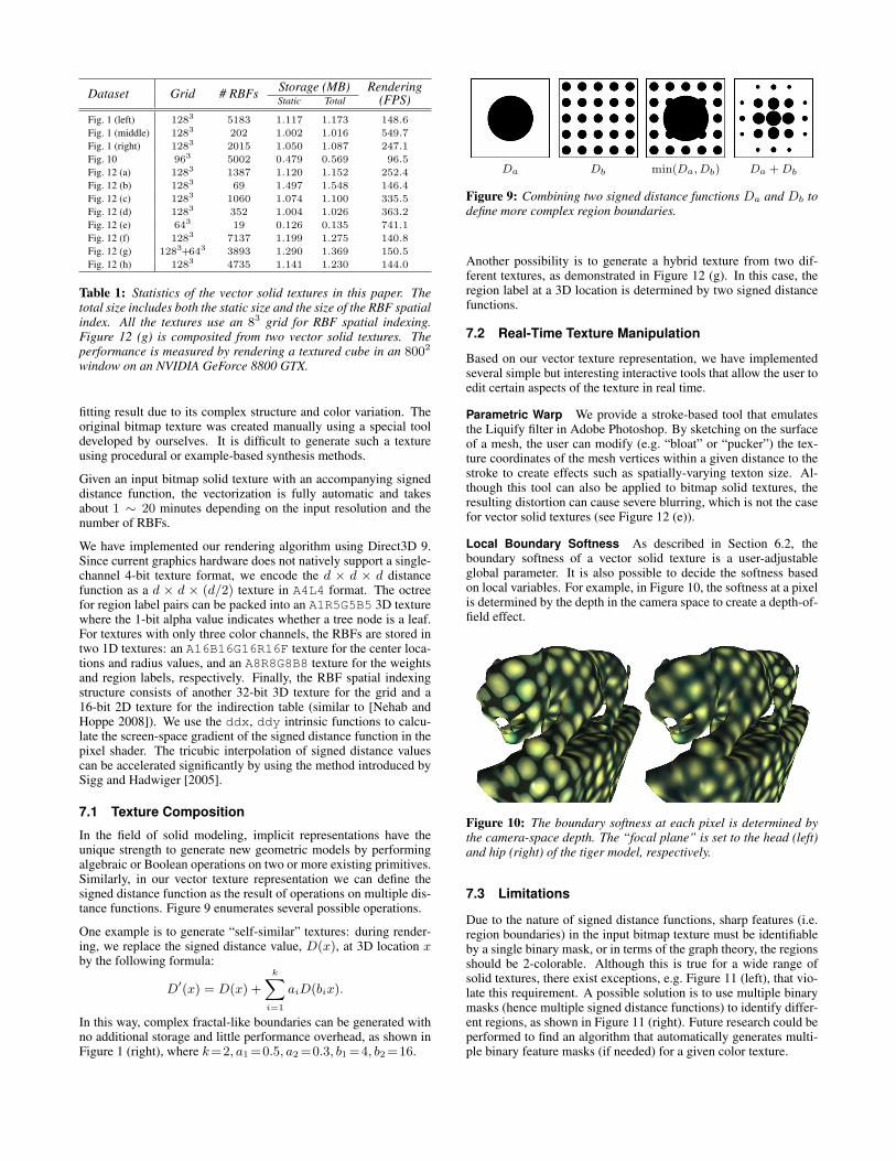
Dataset Grid # RBFs Storage (MB) RenderingStatic Total (FPS)

Fig. 1 (left) 1283 5183 1.117 1.173 148.6

Fig. 1 (middle) 1283 202 1.002 1.016 549.7

Fig. 1 (right) 1283 2015 1.050 1.087 247.1

Fig. 10 963 5002 0.479 0.569 096.5

Fig. 12 (a) 1283 1387 1.120 1.152 252.4

Fig. 12 (b) 1283 69 1.497 1.548 146.4

Fig. 12 (c) 1283 1060 1.074 1.100 335.5

Fig. 12 (d) 1283 352 1.004 1.026 363.2

Fig. 12 (e) 643 19 0.126 0.135 741.1

Fig. 12 (f) 1283 7137 1.199 1.275 140.8

Fig. 12 (g) 1283+643 3893 1.290 1.369 150.5

Fig. 12 (h) 1283 4735 1.141 1.230 144.0

Table 1: Statistics of the vector solid textures in this paper. Thetotal size includes both the static size and the size of the RBF spatialindex. All the textures use an 83 grid for RBF spatial indexing.Figure 12 (g) is composited from two vector solid textures. Theperformance is measured by rendering a textured cube in an 8002

window on an NVIDIA GeForce 8800 GTX.

fitting result due to its complex structure and color variation. Theoriginal bitmap texture was created manually using a special tooldeveloped by ourselves. It is difficult to generate such a textureusing procedural or example-based synthesis methods.

Given an input bitmap solid texture with an accompanying signeddistance function, the vectorization is fully automatic and takesabout 1 ∼ 20 minutes depending on the input resolution and thenumber of RBFs.

We have implemented our rendering algorithm using Direct3D 9.Since current graphics hardware does not natively support a single-channel 4-bit texture format, we encode the d × d × d distancefunction as a d × d × (d/2) texture in A4L4 format. The octreefor region label pairs can be packed into an A1R5G5B5 3D texturewhere the 1-bit alpha value indicates whether a tree node is a leaf.For textures with only three color channels, the RBFs are stored intwo 1D textures: an A16B16G16R16F texture for the center loca-tions and radius values, and an A8R8G8B8 texture for the weightsand region labels, respectively. Finally, the RBF spatial indexingstructure consists of another 32-bit 3D texture for the grid and a16-bit 2D texture for the indirection table (similar to [Nehab andHoppe 2008]). We use the ddx, ddy intrinsic functions to calcu-late the screen-space gradient of the signed distance function in thepixel shader. The tricubic interpolation of signed distance valuescan be accelerated significantly by using the method introduced bySigg and Hadwiger [2005].

7.1 Texture Composition

In the field of solid modeling, implicit representations have theunique strength to generate new geometric models by performingalgebraic or Boolean operations on two or more existing primitives.Similarly, in our vector texture representation we can define thesigned distance function as the result of operations on multiple dis-tance functions. Figure 9 enumerates several possible operations.

One example is to generate “self-similar” textures: during render-ing, we replace the signed distance value, D(x), at 3D location xby the following formula:

D′(x) = D(x) +

k∑i=1

aiD(bix).

In this way, complex fractal-like boundaries can be generated withno additional storage and little performance overhead, as shown inFigure 1 (right), where k=2, a1 =0.5, a2 =0.3, b1 =4, b2 =16.

Da Db min(Da, Db) Da + Db

Figure 9: Combining two signed distance functions Da and Db todefine more complex region boundaries.

Another possibility is to generate a hybrid texture from two dif-ferent textures, as demonstrated in Figure 12 (g). In this case, theregion label at a 3D location is determined by two signed distancefunctions.

7.2 Real-Time Texture Manipulation

Based on our vector texture representation, we have implementedseveral simple but interesting interactive tools that allow the user toedit certain aspects of the texture in real time.

Parametric Warp We provide a stroke-based tool that emulatesthe Liquify filter in Adobe Photoshop. By sketching on the surfaceof a mesh, the user can modify (e.g. “bloat” or “pucker”) the tex-ture coordinates of the mesh vertices within a given distance to thestroke to create effects such as spatially-varying texton size. Al-though this tool can also be applied to bitmap solid textures, theresulting distortion can cause severe blurring, which is not the casefor vector solid textures (see Figure 12 (e)).

Local Boundary Softness As described in Section 6.2, theboundary softness of a vector solid texture is a user-adjustableglobal parameter. It is also possible to decide the softness basedon local variables. For example, in Figure 10, the softness at a pixelis determined by the depth in the camera space to create a depth-of-field effect.

Figure 10: The boundary softness at each pixel is determined bythe camera-space depth. The “focal plane” is set to the head (left)and hip (right) of the tiger model, respectively.

7.3 Limitations

Due to the nature of signed distance functions, sharp features (i.e.region boundaries) in the input bitmap texture must be identifiableby a single binary mask, or in terms of the graph theory, the regionsshould be 2-colorable. Although this is true for a wide range ofsolid textures, there exist exceptions, e.g. Figure 11 (left), that vio-late this requirement. A possible solution is to use multiple binarymasks (hence multiple signed distance functions) to identify differ-ent regions, as shown in Figure 11 (right). Future research could beperformed to find an algorithm that automatically generates multi-ple binary feature masks (if needed) for a given color texture.

Figure 11: In order to achieve a good vectorization of the upperleft texture, two binary masks need to be used.

Another limitation of our method is that boundary softness cannotbe set to an arbitrary value. The upper limit of distance threshold δis determined by the spatial distribution of region label pairs. If δ istoo large, a pixel color could be blended from incorrectly evaluatedregion colors and artifacts may appear.

Since RBF-based color fitting is a lossy procedure, certain high-frequency details in the original bitmap solid texture could besmoothed out. It is worthwhile to investigate how to represent suchdetails in vectorization results.

8 ConclusionWe have introduced a compact random-access vector representa-tion for solid textures. It delivers high-quality rendering results bypreserving both the sharp features and the smooth color variationsof a solid texture. With a spatial indexing structure, our represen-tation enables efficient color evaluation during real-time solid tex-ture mapping. Due to its resolution-independent nature, our repre-sentation supports several interesting applications such as feature-preserving texture composition and parametric warping. We havedeveloped effective techniques to generate vector solid texturesfrom either 2D exemplars or existing bitmap solid textures. Oneinteresting direction for future work is to develop a user-friendlyinterface for designing vector solid textures from scratch.

AcknowledgementsWe would like to thank Johannes Kopf and colleagues for sharing theirdata, Yue Dong and Minmin Gong for providing helpful suggestions, andthe anonymous reviewers for their insightful comments. Some models inthis paper are provided by AIM@SHAPE shape repository and Evermo-tion. Kun Zhou was partially supported by NSFC (No. 60825201), the 973program of China (No. 2009CB320801) and NVIDIA.

References

CHANG, H.-H., AND HONG, Y. 1998. Vectorization of hand-drawn image using piecewise cubic bezier curves fitting. Patternrecognition 31, 11, 1747–1755.

COHEN-STEINER, D., ALLIEZ, P., AND DESBRUN, M. 2004.Variational shape approximation. ACM Trans. Graph. 23, 3,905–914.

DONG, Y., LEFEBVRE, S., TONG, X., AND DRETTAKIS, G. 2008.Lazy solid texture synthesis. Computer Graphics Forum 27, 4,1165–1174.

EBERT, D. S., MUSGRAVE, F. K., PEACHEY, D., PERLIN, K.,AND WORLEY, S. 1994. Texturing and Modeling: A ProceduralApproach. Academic Press.

EFROS, A., AND LEUNG, T. 1999. Texture synthesis by non-parametric sampling. In ICCV ’99, 1033–1038.

FRISKEN, S. F., PERRY, R. N., ROCKWOOD, A. P., AND JONES,T. R. 2000. Adaptively sampled distance fields: a general rep-resentation of shape for computer graphics. In Proceedings ofSIGGRAPH 2000, 249–254.

GHAZANFARPOUR, D., AND DISCHLER, J.-M. 1995. Spectralanalysis for automatic 3-D texture generation. Computers andGraphics 19, 3, 413–422.

GHAZANFARPOUR, D., AND DISCHLER, J.-M. 1996. Genera-tion of 3D texture using multiple 2D model analysis. ComputerGraphics Forum 15, 3, 311–323.

HEEGER, D., AND BERGEN, J. 1995. Pyramid-based texture anal-ysis/synthesis. In Proceedings of SIGGRAPH ’95, 229–238.

HERTZMANN, A., JACOBS, C. E., OLIVER, N., CURLESS, B.,AND SALESIN, D. H. 2001. Image analogies. In Proceedingsof SIGGRAPH 2001, 327–340.

HILAIRE, X., AND TOMBRE, K. 2006. Robust and accurate vec-torization of line drawings. IEEE Trans. Pattern Anal. Mach.Intell. 28, 6, 890–904.

JAGNOW, R., DORSEY, J., AND RUSHMEIER, H. 2004. Stereo-logical techniques for solid textures. ACM Trans. Graph. 23, 3,329–335.

KOPF, J., FU, C.-W., COHEN-OR, D., DEUSSEN, O., LISCHIN-SKI, D., AND WONG, T.-T. 2007. Solid texture synthesis from2D exemplars. ACM Trans. Graph. 26, 3, Article 2.

KWATRA, V., ESSA, I., BOBICK, A., AND KWATRA, N. 2005.Texture optimization for example-based synthesis. ACM Trans.Graph. 24, 3, 795–802.

LAGAE, A., LEFEBVRE, S., DRETTAKIS, G., AND DUTRE, P.2009. Procedural noise using sparse Gabor convolution. ACMTrans. Graph. 28, 3, Article 54.

LAI, Y.-K., HU, S.-M., AND MARTIN, R. 2009. Automatic andtopology-preserving gradient mesh generation for image vector-ization. ACM Trans. Graph. 28, 3, Article 85.

LECOT, G., AND LEVY, B. 2006. Ardeco: Automatic region de-tection and conversion. In EGSR 2006, 349–360.

LEFEBVRE, S., AND HOPPE, H. 2006. Appearance-space texturesynthesis. ACM Trans. Graph. 25, 3, 541–548.

LEFEBVRE, S., HORNUS, S., AND NEYRET, F. 2005. Octreetextures on the GPU. In GPU Gems 2. ch. 37.

NEHAB, D., AND HOPPE, H. 2008. Random-access rendering ofgeneral vector graphics. ACM Trans. Graph. 27, 5, Article 135.

ORZAN, A., BOUSSEAU, A., WINNEMOLLER, H., BARLA, P.,THOLLOT, J., AND SALESIN, D. 2008. Diffusion curves: avector representation for smooth-shaded images. ACM Trans.Graph. 27, 3, Article 92.

PARILOV, E., AND ZORIN, D. 2008. Real-time rendering of tex-tures with feature curves. ACM Trans. Graph. 27, 1, Article 3.

PRICE, B., AND BARRETT, W. 2006. Object-based vectorizationfor interactive image editing. The Visual Computer 22, 9 (sep),661–670.

QIN, X., AND YANG, Y.-H. 2007. Aura 3D textures. IEEE Trans-actions on Visualization and Computer Graphics 13, 2, 379–389.

RAMANARAYANAN, G., BALA, K., AND WALTER, B. 2004.Feature-based textures. In EGSR 2004, 65–73.

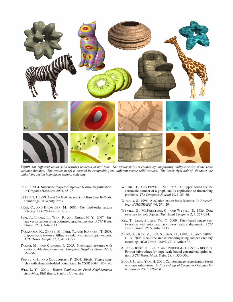
(a) (b) (c) (d)

(e) (f) (g) (h)

Figure 12: Different vector solid textures rendered in real time. The texture in (c) is created by compositing multiple scales of the samedistance function. The texture in (g) is created by compositing two different vector solid textures. The lower right half of (d) shows theunderlying region boundaries without softening.

SEN, P. 2004. Silhouette maps for improved texture magnification.In Graphics Hardware 2004, 65–73.

SETHIAN, J. 1999. Level Set Methods and Fast Marching Methods.Cambridge University Press.

SIGG, C., AND HADWIGER, M. 2005. Fast third-order texturefiltering. In GPU Gems 2. ch. 20.

SUN, J., LIANG, L., WEN, F., AND SHUM, H.-Y. 2007. Im-age vectorization using optimized gradient meshes. ACM Trans.Graph. 26, 3, Article 11.

TAKAYAMA, K., OKABE, M., IJIRI, T., AND IGARASHI, T. 2008.Lapped solid textures: filling a model with anisotropic textures.ACM Trans. Graph. 27, 3, Article 53.

TARINI, M., AND CIGNONI, P. 2005. Pinchmaps: textures withcustomizable discontinuities. Computer Graphics Forum 24, 3,557–568.

TUMBLIN, J., AND CHOUDHURY, P. 2004. Bixels: Picture sam-ples with sharp embedded boundaries. In EGSR 2004, 186–196.

WEI, L.-Y. 2001. Texture Synthesis by Fixed NeighborhoodSearching. PhD thesis, Stanford University.

WELSH, D., AND POWELL, M. 1967. An upper bound for thechromatic number of a graph and its application to timetablingproblems. The Computer Journal 10, 1, 85–86.

WORLEY, S. 1996. A cellular texture basis function. In Proceed-ings of SIGGRAPH ’96, 291–294.

WYVILL, G., MCPHEETERS, C., AND WYVILL, B. 1986. Datastructure for soft objects. The Visual Computer 2, 4, 227–234.

XIA, T., LIAO, B., AND YU, Y. 2009. Patch-based image vec-torization with automatic curvilinear feature alignment. ACMTrans. Graph. 28, 5, Article 115.

ZHOU, K., REN, Z., LIN, S., BAO, H., GUO, B., AND SHUM,H.-Y. 2008. Real-time smoke rendering using compensated raymarching. ACM Trans. Graph. 27, 3, Article 36.

ZHU, C., BYRD, R., LU, P., AND NOCEDAL, J. 1997. L-BFGS-B:Fortran subroutines for large-scale bound constrained optimiza-tion. ACM Trans. Math. Softw. 23, 4, 550–560.

ZOU, J. J., AND YAN, H. 2001. Cartoon image vectorization basedon shape subdivision. In Proceedings of Computer Graphics In-ternational 2001, 225–231.