dynamo regimes with a nonhelical forcing

DYNAMO REGIMES WITH A NONHELICAL FORCING

Pablo D. Mininni,1Yannick Ponty,

2David C. Montgomery,

3Jean-Francois Pinton,

4

Helene Politano,2and Annick Pouquet

1

Received 2004 December 2; accepted 2005 February 24

ABSTRACT

A three-dimensional numerical computation of magnetohydrodynamic dynamo behavior is described. The dynamois mechanically forced with a driving term of the Taylor-Green type. The magnetic field development is followed fromnegligibly small levels to saturated values that occur at magnetic energies comparable to the kinetic energies. Althoughthere is locally a nonzero helicity density, there is no overall integrated helicity in the system. Persistent oscillations areobserved in the saturated state for not-too-large mechanical Reynolds numbers, oscillations in which the kinetic andmagnetic energies vary out of phase but with no reversal of the magnetic field. The flow pattern exhibits considerablegeometrical structure in this regime. As the Reynolds number is increased, the oscillations disappear and the energiesbecome more nearly stationary, but retain some unsystematically fluctuating turbulent time dependence. The regulargeometrical structure of the fields gives way to a more spatially disordered distribution. The injection and dissipationscales are identified, and the different components of energy transfer in Fourier space are analyzed, particularly in thecontext of clarifying the role played by different flow scales in the amplification of the magnetic field. We observe thatsmall and large scales interact and contribute to the dynamo process.

Subject headinggs: magnetic fields — MHD

Online material: color figures

1. INTRODUCTION

Evidence of the existence of magnetic fields is known in manyastronomical objects. These fields are believed to be generatedand sustained by a dynamo process (e.g., Moffatt 1978), andoften these objects are characterized by the presence of large-scale flows (such as rotation) and turbulent fluctuations. Thesetwo ingredients are known to be often associated with magneto-hydrodynamic dynamos. In recent years, significant advanceshave been made either studying large-scale flow dynamos in thekinematic approximation or using direct numerical simulationsto study turbulent amplification of magnetic fields in simplifiedgeometries.

In a previous paper (Ponty et al. 2005), a study of the self-generation of magnetic fields in a turbulent conducting fluidwas reported. The study was computational and dealt mainlywith the effects of lowering the magnetic Prandtl number PM

of the fluid (ratio of kinematic viscosity to magnetic diffusivity).The velocity field was externally excited by a forcing term on theright-hand side of the equation of motion whose geometry wasthat of what has come to be called the Taylor-Green vortex(Taylor & Green 1937; Morf et al. 1980; Pelz et al. 1985; Noreet al. 1997; Marie et al. 2003; Bourgoin et al. 2004). The regimeof operation was one of kinetic Reynolds number 31 (so thatthe fluid motions were turbulent), and the emphasis was on howlarge the magnetic Reynolds numbers had to be for the infini-tesimal magnetic fields to be amplified and grow to macroscopicvalues.

Here, we want to describe and stress another aspect of theTaylor-Green dynamo. In particular, we have found computation-

ally that it has an oscillatory regime, for not too large a Reynoldsnumber, in which energy is passed back and forth regularly be-tween the mechanical motions and the magnetic excitations in away we believe to be new. Out of the velocity field emerges ageometrically regular, time-averaged pattern involving coherentmagnetic and mechanical oscillations.

As the Reynolds number is increased, the resulting flow has awell-defined large-scale pattern and nonhelical turbulent fluctua-tions. In this case, the oscillations disappear, and the magneticfield grows at scales both larger and smaller than the integral scaleof the flow. After the nonlinear saturation of the dynamo, veloc-ity field fluctuations are partially suppressed, and a magnetic fieldwith a spatial pattern reminiscent of the low Reynolds numbercase can be identified. This complex evolution of the magneticfield can be understood by studying the role played by the energytransfer in Fourier space.

In x 2, we describe the numerical experiments and outline atypical time history of the development of an oscillatory dy-namo. We then go on to show how, by increasing the Reynoldsnumber, the oscillatory behavior can be suppressed. In x 3, wemake use of color displays of the field quantities to demonstratethe cycle of the oscillation and to reveal the intriguing and com-plex varying three-dimensional pattern that characterizes it. Thepattern, although regular, is difficult to see through completelyin physical terms. Finally, x 4 suggests some precedents, pro-vides a partial explanation, and considers other similar situationsin which such coherence may or may not be expected to emergeout of turbulent disorder.

2. THE COMPUTATION

The Taylor-Green vortex is a flow with an initial periodicvelocity field

vTG(k0)¼sin k0xð Þ cos k0yð Þ cos k0zð Þ�cos k0xð Þ sin k0yð Þ cos k0zð Þ

0

264

375 ð1Þ

1 National Center for Atmospheric Research, P.O. Box 3000, Boulder, CO80307-3000.

2 Laboratoire Cassiopee, CNRSUMR6203, Observatoire de la Cote d’Azur,BP 4229, F-06034 Nice Cedex 04, France.

3 Department of Physics and Astronomy, 6127 Wilder Laboratory, DartmouthCollege, Hanover, NH 03755.

4 Laboratoire de Physique, CNRS UMR5672, Ecole Normale Superieure deLyon, 46 Allee d’Italie, 69007 Lyon, France.

A

853

The Astrophysical Journal, 626:853–863, 2005 June 20

# 2005. The American Astronomical Society. All rights reserved. Printed in U.S.A.

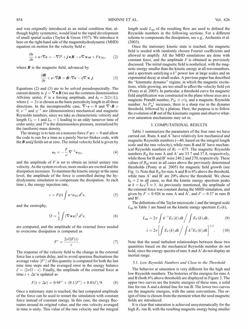
and was originally introduced as an initial condition that, al-though highly symmetric, would lead to the rapid developmentof small spatial scales (Taylor & Green 1937). We introduce ithere on the right-hand side of the magnetohydrodynamic (MHD)equation on motion for the velocity field v:

@v

@tþ v =:v ¼ �:P þ j<B� �:<wþ FvTG; ð2Þ

where B is the magnetic field, advanced by

@B

@tþ v =:B ¼ B = :v� �: < j: ð3Þ

Equations (2) and (3) are to be solved pseudospectrally. Thecurrent density is j ¼ :<B (we use the common dimensionlessAlfvenic units), F is a forcing amplitude, and k0 ¼ 2(2� /L),where L ¼ 2� is chosen as the basic periodicity length in all threedirections. In the incompressible case, := v ¼ 0 and :=B ¼0; ��1 and ��1 are (dimensionless) mechanical and magneticReynolds numbers, since we take as characteristic velocity andlength U0 ¼ 1 and L0 ¼ 1 leading to an eddy turnover time oforder unity; andP is the dimensionless pressure, normalized bythe (uniform) mass density.

The strategy is to turn on a nonzero force F at t ¼ 0 and allowthe code to run for a time as a purely Navier-Stokes code, withtheB and j fields set at zero. The initial velocity field is given by

v0 ¼ � F

�:�2vTG; ð4Þ

and the amplitude of F is set to obtain an initial unitary rmsvelocity. As the system evolves, more modes are excited and thedissipation increases. Tomaintain the kinetic energy at the samelevel, the amplitude of the force is controlled during the hy-drodynamic simulation to compensate the dissipation. At eachtime t, the energy injection rate,

� ¼ F(t)

Zv = vTG d3x; ð5Þ

and the enstrophy,

� ¼ 1

2

Z:< vð Þ2 d3x; ð6Þ

are computed, and the amplitude of the external force neededto overcome dissipation is computed as

F� ¼ 2��F tð Þ�

: ð7Þ

The response of the velocity field to the change in the externalforce has a certain delay, and to avoid spurious fluctuations theaverage value hF�i of this quantity is computed for both the lastnine time steps and the averaged error in the energy balanceE ¼ h2�� i. Finally, the amplitude of the external force attime t þ�t is updated as

F t þ�tð Þ ¼ 0:9F� þ 0:1 F�h i þ 0:01Eð Þ=9: ð8Þ

Once a stationary state is reached, the last computed amplitudeof the force can be used to restart the simulation with constantforce instead of constant energy. In this case, the energy fluc-tuates around its original value, and the rms velocity averagedin time is unity. This value of the rms velocity and the integral

length scale Lint of the resulting flow are used to defined theReynolds numbers in the following sections. For a differentscheme to compensate the dissipation, see e.g., Archontis et al.(2003).Once the stationary kinetic state is reached, the magnetic

field is seeded with randomly chosen Fourier coefficients andallowed to amplify. All the MHD simulations are done withconstant force, and the amplitude F is obtained as previouslydiscussed. The initial magnetic field is nonhelical, with the mag-netic energy smaller than the kinetic energy at all wavenumbers,and a spectrum satisfying a k2 power law at large scales and anexponential decay at small scales. A previous paper has describedthe ‘‘kinematic dynamo’’ regime, in which the magnetic excita-tions, while growing, are too small to affect the velocity field yet(Ponty et al. 2005). In particular, a threshold curve for magneticfield amplification was constructed in the plane whose axes are amagnetic Prandtl number, PM � �/�, and a magnetic Reynoldsnumber. As P�1

M increases, there is a sharp rise in the dynamothreshold, followed by a plateau. Here, the purpose is to followthe evolution ofB out of the kinematic regime and observe what-ever saturation mechanisms may set in.

3. COMPUTATIONAL RESULTS

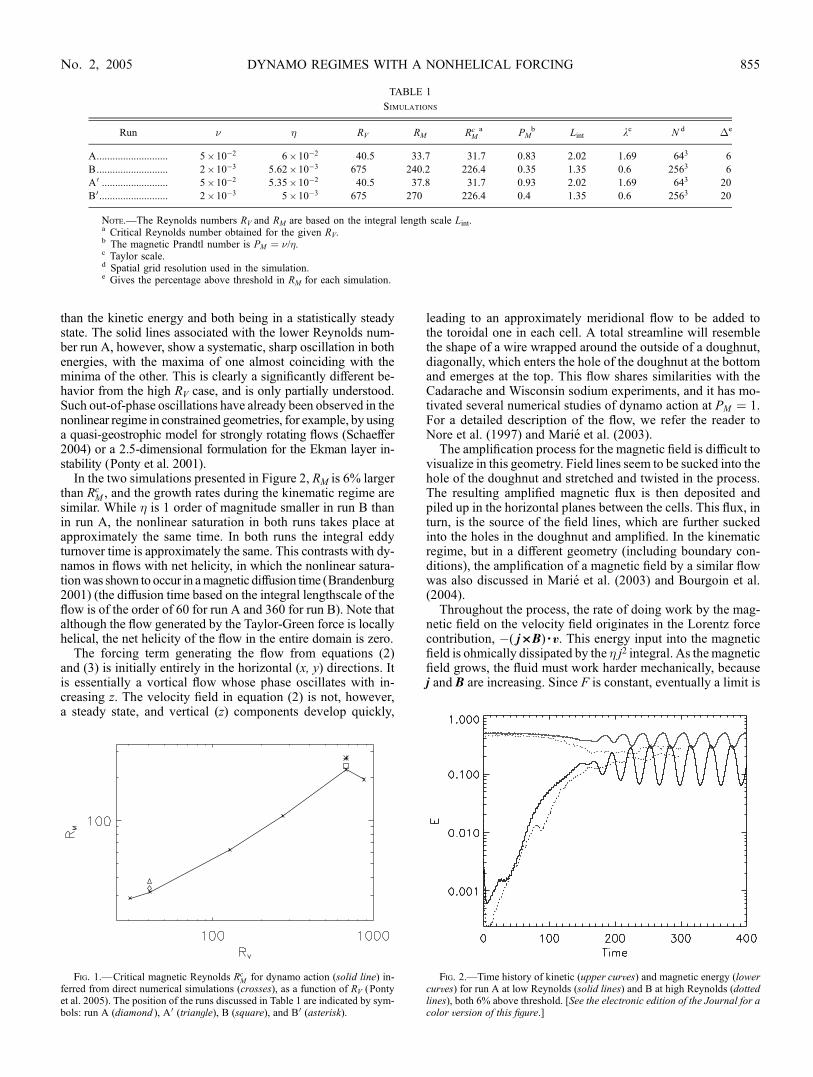
Table 1 summarizes the parameters of the four runs we havecarried out. Runs A and A 0 have relatively low mechanical andmagnetic Reynolds numbers (�40, based on the integral lengthscale and the rms velocity), while runs B and B0 have mechan-ical Reynolds numbers of RV ¼ 675. The magnetic Reynoldsnumbers RM for runs A and A 0 are 33.7 and 37.8, respectively,while those for B and B0 were 240.2 and 270, respectively. Thesevalues of RM were in all cases above the previously determinedthresholds (Ponty et al. 2005) for magnetic field growth (seeFig. 1). Note that RM for runs A and B is 6% above the threshold,while runs A0 and B0 are 20% above the threshold. We chosek0 ¼ 2 in all cases, so that the kinetic energy spectrum peaksat k ¼ k0

ffiffiffi3

p� 3. As previously mentioned, the amplitude of

the external force was constant during the MHD simulation, andgiven by F ¼ 0:926 in runs A and A0, and F ¼ 0:37 in runs Band B0.The definitions of the Taylor microscale k and the integral scale

Lint in Table 1 are based on the kinetic energy spectrum EV (k),

Lint ¼ 2�

Zk�1EV kð Þ dk

�ZEV kð Þ dk; ð9Þ

k ¼ 2�

ZEV kð Þ dk

�Zk 2EV kð Þ dk

� �1=2: ð10Þ

Note that the usual turbulent relationships between these twoquantities based on the mechanical Reynolds number do nothold, since the energy spectra of runs A and A0 do not display aninertial range.

3.1. Low Reynolds Numbers and Close to the Threshold

The behavior at saturation is very different for the high andlow Reynolds numbers. The histories of the energies for runs Aand B (both 6% above threshold) are displayed in Figure 2. Theupper two curves are the kinetic energies of these runs, a solidline for run A and a dotted line for run B. The lower two curvesare the magnetic energies, with the same conventions. The or-igin of time is chosen from the moment when the seed magneticfields are introduced.It is clear that saturation is achieved unsystematically for the

high RV run B, with the resulting magnetic energy being smaller

MININNI ET AL.854 Vol. 626

than the kinetic energy and both being in a statistically steadystate. The solid lines associated with the lower Reynolds num-ber run A, however, show a systematic, sharp oscillation in bothenergies, with the maxima of one almost coinciding with theminima of the other. This is clearly a significantly different be-havior from the high RV case, and is only partially understood.Such out-of-phase oscillations have already been observed in thenonlinear regime in constrained geometries, for example, by usinga quasi-geostrophic model for strongly rotating flows (Schaeffer2004) or a 2.5-dimensional formulation for the Ekman layer in-stability (Ponty et al. 2001).

In the two simulations presented in Figure 2, RM is 6% largerthan Rc

M , and the growth rates during the kinematic regime aresimilar. While � is 1 order of magnitude smaller in run B thanin run A, the nonlinear saturation in both runs takes place atapproximately the same time. In both runs the integral eddyturnover time is approximately the same. This contrasts with dy-namos in flows with net helicity, in which the nonlinear satura-tionwas shown to occur in amagnetic diffusion time (Brandenburg2001) (the diffusion time based on the integral lengthscale of theflow is of the order of 60 for run A and 360 for run B). Note thatalthough the flow generated by the Taylor-Green force is locallyhelical, the net helicity of the flow in the entire domain is zero.

The forcing term generating the flow from equations (2)and (3) is initially entirely in the horizontal (x, y) directions. Itis essentially a vortical flow whose phase oscillates with in-creasing z. The velocity field in equation (2) is not, however,a steady state, and vertical (z) components develop quickly,

leading to an approximately meridional flow to be added tothe toroidal one in each cell. A total streamline will resemblethe shape of a wire wrapped around the outside of a doughnut,diagonally, which enters the hole of the doughnut at the bottomand emerges at the top. This flow shares similarities with theCadarache and Wisconsin sodium experiments, and it has mo-tivated several numerical studies of dynamo action at PM ¼ 1.For a detailed description of the flow, we refer the reader toNore et al. (1997) and Marie et al. (2003).

The amplification process for the magnetic field is difficult tovisualize in this geometry. Field lines seem to be sucked into thehole of the doughnut and stretched and twisted in the process.The resulting amplified magnetic flux is then deposited andpiled up in the horizontal planes between the cells. This flux, inturn, is the source of the field lines, which are further suckedinto the holes in the doughnut and amplified. In the kinematicregime, but in a different geometry (including boundary con-ditions), the amplification of a magnetic field by a similar flowwas also discussed in Marie et al. (2003) and Bourgoin et al.(2004).

Throughout the process, the rate of doing work by the mag-netic field on the velocity field originates in the Lorentz forcecontribution, �( j<B) = v. This energy input into the magneticfield is ohmically dissipated by the � j2 integral. As the magneticfield grows, the fluid must work harder mechanically, becausej and B are increasing. Since F is constant, eventually a limit is

Fig. 1.—Critical magnetic Reynolds RcM for dynamo action (solid line) in-

ferred from direct numerical simulations (crosses), as a function of RV (Pontyet al. 2005). The position of the runs discussed in Table 1 are indicated by sym-bols: run A (diamond ), A 0 (triangle), B (square), and B0 (asterisk).

TABLE 1

Simulations

Run � � RV RM RcMa PM

b Lint kc N d �e

A........................... 5 ; 10�2 6 ; 10�2 40.5 33.7 31.7 0.83 2.02 1.69 643 6

B........................... 2 ; 10�3 5:62 ; 10�3 675 240.2 226.4 0.35 1.35 0.6 2563 6

A0 ......................... 5 ; 10�2 5:35 ; 10�2 40.5 37.8 31.7 0.93 2.02 1.69 643 20

B0 .......................... 2 ; 10�3 5 ; 10�3 675 270 226.4 0.4 1.35 0.6 2563 20

Note.—The Reynolds numbers RV and RM are based on the integral length scale Lint.a Critical Reynolds number obtained for the given RV.b The magnetic Prandtl number is PM ¼ �/�.c Taylor scale.d Spatial grid resolution used in the simulation.e Gives the percentage above threshold in RM for each simulation.

Fig. 2.—Time history of kinetic (upper curves) and magnetic energy (lowercurves) for run A at low Reynolds (solid lines) and B at high Reynolds (dottedlines), both 6% above threshold. [See the electronic edition of the Journal for acolor version of this figure.]

DYNAMO REGIMES WITH A NONHELICAL FORCING 855No. 2, 2005

reached at which v can no longer transfer energy to B at itsprevious rate and slows down. At that point, the magnetic en-ergy begins to be transferred in the reverse sense, so that vgrows again as j and B become weaker. The cyclic nature of theprocess ensues.

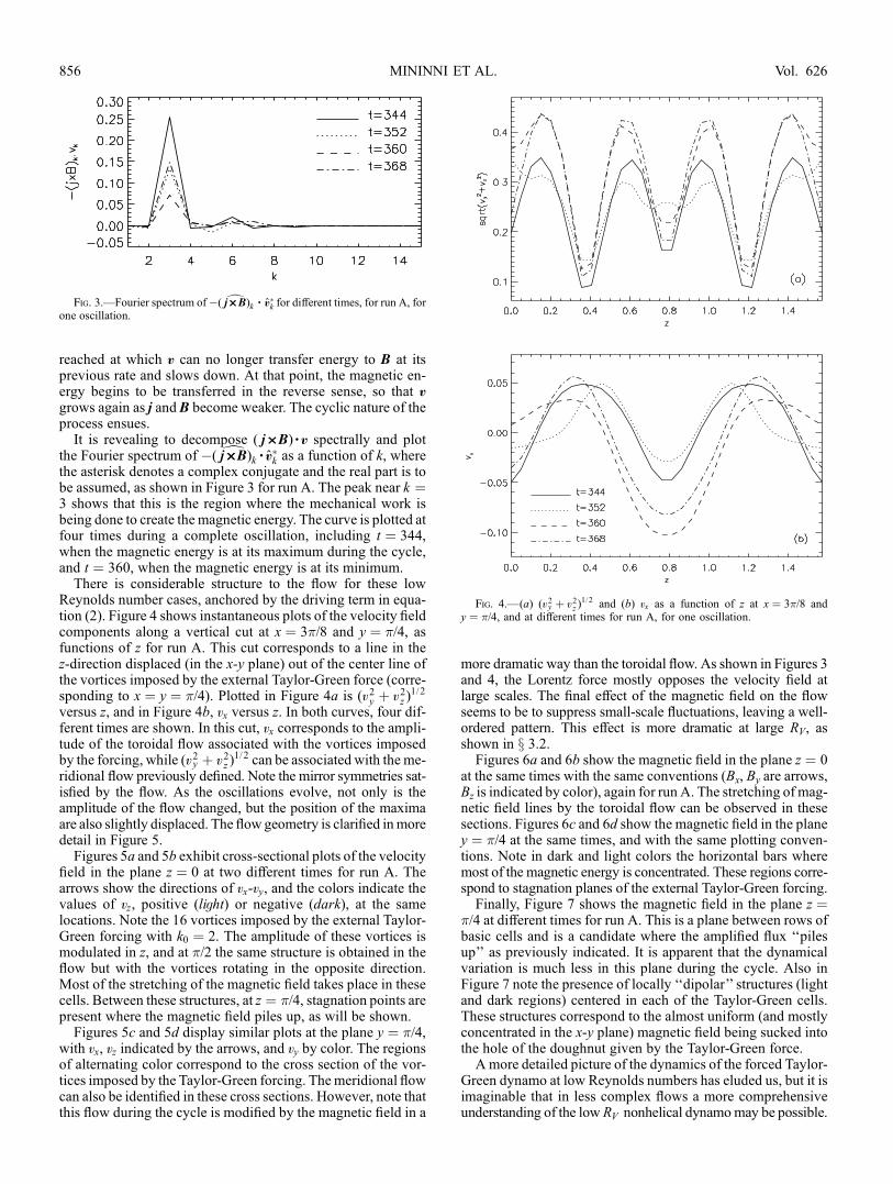
It is revealing to decompose ( j<B) = v spectrally and plotthe Fourier spectrum of �( dj��B)k = v

�k as a function of k, where

the asterisk denotes a complex conjugate and the real part is tobe assumed, as shown in Figure 3 for run A. The peak near k ¼3 shows that this is the region where the mechanical work isbeing done to create the magnetic energy. The curve is plotted atfour times during a complete oscillation, including t ¼ 344,when the magnetic energy is at its maximum during the cycle,and t ¼ 360, when the magnetic energy is at its minimum.

There is considerable structure to the flow for these lowReynolds number cases, anchored by the driving term in equa-tion (2). Figure 4 shows instantaneous plots of the velocity fieldcomponents along a vertical cut at x ¼ 3�/8 and y ¼ �/4, asfunctions of z for run A. This cut corresponds to a line in thez-direction displaced (in the x-y plane) out of the center line ofthe vortices imposed by the external Taylor-Green force (corre-sponding to x ¼ y ¼ �/4). Plotted in Figure 4a is (v2y þ v 2z )

1=2

versus z, and in Figure 4b, vx versus z. In both curves, four dif-ferent times are shown. In this cut, vx corresponds to the ampli-tude of the toroidal flow associated with the vortices imposedby the forcing, while (v2y þ v 2z )

1=2 can be associated with the me-ridional flow previously defined. Note the mirror symmetries sat-isfied by the flow. As the oscillations evolve, not only is theamplitude of the flow changed, but the position of the maximaare also slightly displaced. The flow geometry is clarified inmoredetail in Figure 5.

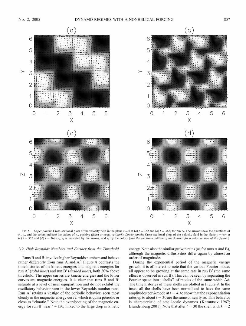
Figures 5a and 5b exhibit cross-sectional plots of the velocityfield in the plane z ¼ 0 at two different times for run A. Thearrows show the directions of vx-vy, and the colors indicate thevalues of vz, positive (light) or negative (dark), at the samelocations. Note the 16 vortices imposed by the external Taylor-Green forcing with k0 ¼ 2. The amplitude of these vortices ismodulated in z, and at �/2 the same structure is obtained in theflow but with the vortices rotating in the opposite direction.Most of the stretching of the magnetic field takes place in thesecells. Between these structures, at z ¼ �/4, stagnation points arepresent where the magnetic field piles up, as will be shown.

Figures 5c and 5d display similar plots at the plane y ¼ �/4,with vx, vz indicated by the arrows, and vy by color. The regionsof alternating color correspond to the cross section of the vor-tices imposed by the Taylor-Green forcing. Themeridional flowcan also be identified in these cross sections. However, note thatthis flow during the cycle is modified by the magnetic field in a

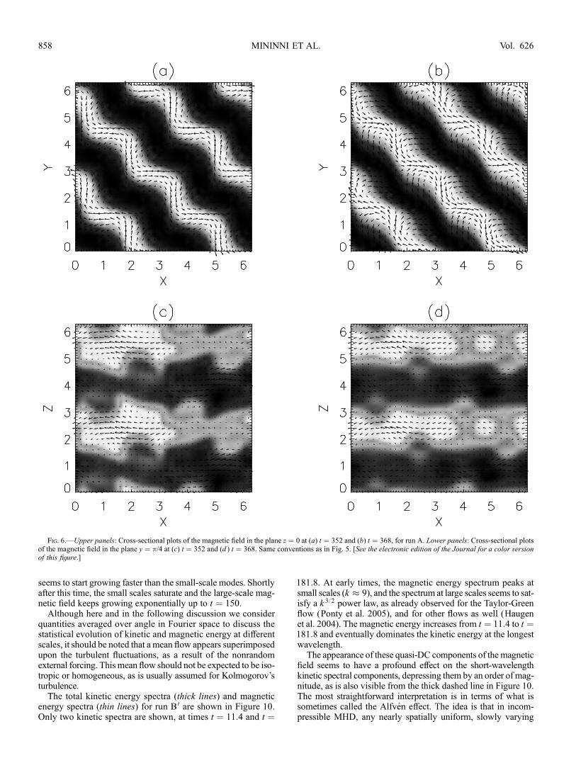
more dramatic way than the toroidal flow. As shown in Figures 3and 4, the Lorentz force mostly opposes the velocity field atlarge scales. The final effect of the magnetic field on the flowseems to be to suppress small-scale fluctuations, leaving a well-ordered pattern. This effect is more dramatic at large RV, asshown in x 3.2.Figures 6a and 6b show the magnetic field in the plane z ¼ 0

at the same times with the same conventions (Bx, By are arrows,Bz is indicated by color), again for run A. The stretching of mag-netic field lines by the toroidal flow can be observed in thesesections. Figures 6c and 6d show the magnetic field in the planey ¼ �/4 at the same times, and with the same plotting conven-tions. Note in dark and light colors the horizontal bars wheremost of the magnetic energy is concentrated. These regions corre-spond to stagnation planes of the external Taylor-Green forcing.Finally, Figure 7 shows the magnetic field in the plane z ¼

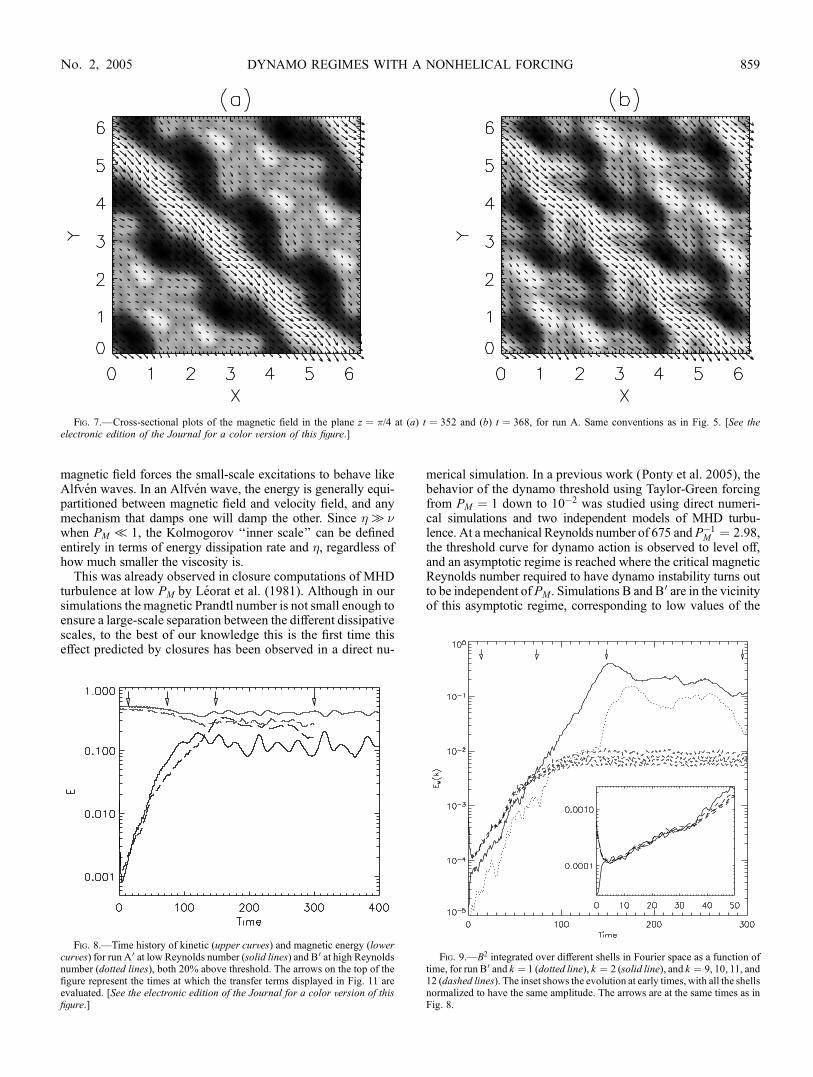
�/4 at different times for run A. This is a plane between rows ofbasic cells and is a candidate where the amplified flux ‘‘pilesup’’ as previously indicated. It is apparent that the dynamicalvariation is much less in this plane during the cycle. Also inFigure 7 note the presence of locally ‘‘dipolar’’ structures (lightand dark regions) centered in each of the Taylor-Green cells.These structures correspond to the almost uniform (and mostlyconcentrated in the x-y plane) magnetic field being sucked intothe hole of the doughnut given by the Taylor-Green force.A more detailed picture of the dynamics of the forced Taylor-

Green dynamo at low Reynolds numbers has eluded us, but it isimaginable that in less complex flows a more comprehensiveunderstanding of the low RV nonhelical dynamomay be possible.

Fig. 3.—Fourier spectrum of�( dj��B)k = v�k for different times, for run A, for

one oscillation.

Fig. 4.—(a) (v2y þ v2z )1=2 and (b) vx as a function of z at x ¼ 3�/8 and

y ¼ �/4, and at different times for run A, for one oscillation.


3.2. High Reynolds Numbers and Farther from the Threshold

Runs B and B 0 involve higher Reynolds numbers and behaverather differently from runs A and A 0. Figure 8 contrasts thetime histories of the kinetic energies and magnetic energies forrun A 0 (solid lines) and run B0 (dashed lines), both 20% abovethreshold. The upper curves are kinetic energies and the lowercurves are magnetic energies. It is clear that runs B and B0

saturate at a level of near equipartition and do not exhibit theoscillatory behavior seen in the lower Reynolds number runs.Run A 0 retains a vestige of the periodic behavior, seen mostclearly in the magnetic energy curve, which is quasi periodic orclose to ‘‘chaotic.’’ Note the overshooting of the magnetic en-ergy for run B 0 near t �150, linked to the large drop in kinetic

energy. Note also the similar growth rates (as for runs A and B),although the magnetic diffusivities differ again by almost anorder of magnitude.

During the exponential period of the magnetic energygrowth, it is of interest to note that the various Fourier modesall appear to be growing at the same rate in run B 0 (the sameeffect is observed in run B). This can be seen by separating theFourier space into ‘‘shells’’ of modes of the same width �k.The time histories of these shells are plotted in Figure 9. In theinset, all the shells have been normalized to have the sameamplitudes per k-mode at t ¼ 4, to show that the exponentiationrates up to about t ¼ 30 are the same or nearly so. This behavioris characteristic of small-scale dynamos (Kazantsev 1967;Brandenburg 2001). Note that after t ¼ 30 the shell with k ¼ 2

Fig. 5.—Upper panels: Cross-sectional plots of the velocity field in the plane z¼ 0 at (a) t ¼ 352 and (b) t ¼ 368, for run A. The arrows show the directions ofvx, vy, and the colors indicate the values of vz, positive (light) or negative (dark). Lower panels: Cross-sectional plots of the velocity field in the plane y ¼ �/4 at(c) t ¼ 352 and (d ) t ¼ 368 (vx, vz is indicated by the arrows, and vy by the color). [See the electronic edition of the Journal for a color version of this figure.]


seems to start growing faster than the small-scale modes. Shortlyafter this time, the small scales saturate and the large-scale mag-netic field keeps growing exponentially up to t ¼ 150.

Although here and in the following discussion we considerquantities averaged over angle in Fourier space to discuss thestatistical evolution of kinetic and magnetic energy at differentscales, it should be noted that a mean flow appears superimposedupon the turbulent fluctuations, as a result of the nonrandomexternal forcing. This mean flow should not be expected to be iso-tropic or homogeneous, as is usually assumed for Kolmogorov’sturbulence.

The total kinetic energy spectra (thick lines) and magneticenergy spectra (thin lines) for run B 0 are shown in Figure 10.Only two kinetic spectra are shown, at times t ¼ 11:4 and t ¼

181:8. At early times, the magnetic energy spectrum peaks atsmall scales (k � 9), and the spectrum at large scales seems to sat-isfy a k 3=2 power law, as already observed for the Taylor-Greenflow (Ponty et al. 2005), and for other flows as well (Haugenet al. 2004). The magnetic energy increases from t ¼ 11:4 to t ¼181:8 and eventually dominates the kinetic energy at the longestwavelength.The appearance of these quasi-DC components of the magnetic

field seems to have a profound effect on the short-wavelengthkinetic spectral components, depressing them by an order of mag-nitude, as is also visible from the thick dashed line in Figure 10.The most straightforward interpretation is in terms of what issometimes called the Alfven effect. The idea is that in incom-pressible MHD, any nearly spatially uniform, slowly varying

Fig. 6.—Upper panels: Cross-sectional plots of the magnetic field in the plane z ¼ 0 at (a) t ¼ 352 and (b) t ¼ 368, for run A. Lower panels: Cross-sectional plotsof the magnetic field in the plane y ¼ �/4 at (c) t ¼ 352 and (d ) t ¼ 368. Same conventions as in Fig. 5. [See the electronic edition of the Journal for a color versionof this figure.]


magnetic field forces the small-scale excitations to behave likeAlfven waves. In an Alfven wave, the energy is generally equi-partitioned between magnetic field and velocity field, and anymechanism that damps one will damp the other. Since �3 �when PMT1, the Kolmogorov ‘‘inner scale’’ can be definedentirely in terms of energy dissipation rate and �, regardless ofhow much smaller the viscosity is.

This was already observed in closure computations of MHDturbulence at low PM by Leorat et al. (1981). Although in oursimulations the magnetic Prandtl number is not small enough toensure a large-scale separation between the different dissipativescales, to the best of our knowledge this is the first time thiseffect predicted by closures has been observed in a direct nu-

merical simulation. In a previous work (Ponty et al. 2005), thebehavior of the dynamo threshold using Taylor-Green forcingfrom PM ¼ 1 down to 10�2 was studied using direct numeri-cal simulations and two independent models of MHD turbu-lence. At a mechanical Reynolds number of 675 and P�1

M ¼ 2:98,the threshold curve for dynamo action is observed to level off,and an asymptotic regime is reached where the critical magneticReynolds number required to have dynamo instability turns outto be independent of PM . Simulations B and B0 are in the vicinityof this asymptotic regime, corresponding to low values of the

Fig. 7.—Cross-sectional plots of the magnetic field in the plane z ¼ �/4 at (a) t ¼ 352 and (b) t ¼ 368, for run A. Same conventions as in Fig. 5. [See theelectronic edition of the Journal for a color version of this figure.]

Fig. 8.—Time history of kinetic (upper curves) and magnetic energy (lowercurves) for run A 0 at low Reynolds number (solid lines) and B 0 at high Reynoldsnumber (dotted lines), both 20% above threshold. The arrows on the top of thefigure represent the times at which the transfer terms displayed in Fig. 11 areevaluated. [See the electronic edition of the Journal for a color version of thisfigure.]

Fig. 9.—B2 integrated over different shells in Fourier space as a function oftime, for run B 0 and k ¼ 1 (dotted line), k ¼ 2 (solid line), and k ¼ 9, 10, 11, and12 (dashed lines). The inset shows the evolution at early times, with all the shellsnormalized to have the same amplitude. The arrows are at the same times as inFig. 8.


magnetic Prandtl number. For a different external forcing (see,e.g., Schekochihin et al. [2004] and Haugen et al. [2004] for theimplications of a purely random and nonhelical force), the as-ymptotic behavior as a function of PM can differ.

Note that with high Reynolds numbers, in the pure hydro-dynamic case, excitations will go farther out in k space. Butonce a large-scale magnetic field is present, if small scales be-have like an approximately equipartitioned Alfven wave, thelarger transport coefficient will drain both the v and B fields (re-sistivity in this case). One could jump to the conclusion that for�/�T1, the dynamo process will behave as if PMwere ofO(1)at all times (see Yousef et al. [2003] for different simulationssupporting this conclusion). We warn that this is certainly in-appropriate in the formation, or kinematic phase, when the mag-netic field is small but amplifying, and there is no quasi-DCmagnetic field to enforce the necessary approximate equipar-tition at small scales. This warning can also apply in more com-plex systems, such as during the reversals of the Earth’s dynamo.

The central role played by the �v = ( j<B) term by whichenergy is extracted from the velocity field can be clarified byplotting the transfer functions T(k) for the magnetic field andvelocity field as functions of k at different times.

The energy transfer function

T kð Þ ¼ TV kð Þ þ TM kð Þ ð11Þ

represents the transfer of energy in k-space and is obtained bydotting the Fourier transform of the nonlinear terms in themomentum equation (2) and in the induction equation (3) by theFourier transform of v and B, respectively. It also satisfies

0 ¼Z 1

0

T k 0ð Þ dk 0; ð12Þ

because of energy conservation by the nonlinear terms; onecan also define

� kð Þ ¼Z k

0

T k 0ð Þ dk 0; ð13Þ

where�(k) is the energy flux in Fourier space. In equation (11),TV (k) is the transfer of kinetic energy

TV kð Þ ¼Z

vk = � bw< vð Þk þ bj<B� �k

h i�d�k ; ð14Þ

where the hat denotes Fourier transform, the asterisk com-plex conjugate, and d�k denotes integration over angle in Fourierspace. In this equation and the following, it is assumed that thecomplex conjugate of the integral is added to obtain a real transferfunction.The transfer of magnetic energy is given by

TM kð Þ ¼Z

Bk =:< bv<B� ��

kd�k ; ð15Þ

and we can also define the transfer of energy due to the Lorentzforce,

TL kð Þ ¼Z

vk = bj<B� ��

kd�k : ð16Þ

Note that this latter term is part of TV (k); it gives an estimation ofthe alignment between the velocity field and the Lorentz force ateach Fourier shell (as shown previously in Fig. 3). This termalso represents energy that is transferred from the kinetic res-ervoir to the magnetic reservoir [in the steady state, the integralover all k of TL(k) is equal to the magnetic energy dissipationrate, as follows from eq. (3)].Figure 11 shows the transfer functions T(k; t ¼ 0), which

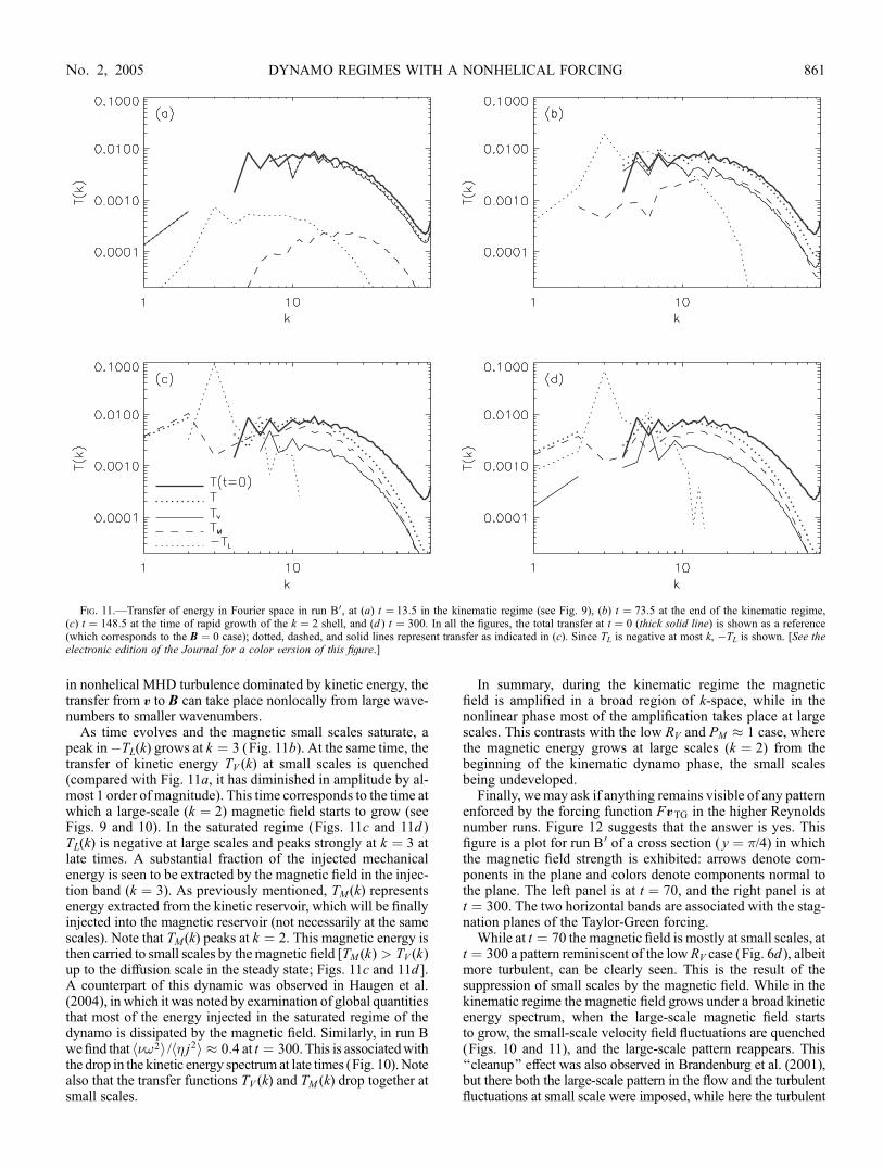
corresponds to the total energy transfer in the hydrodynamicsimulation, since the magnetic seed has just been introduced;T(k), which is the total energy transfer; TV (k); TM (k); and�TL(k),as functions of k for four different times for run B0. A gap in oneof the spectra indicates (since the plotting is logarithmic) that ithas changed sign. It is apparent that the dominant transfer isalways in the vicinity of the forcing band, although it is quitespread over all wavenumbers in the inertial range at all times. It isalso apparent that at the later times, most of the transfer is mag-netic transfer, in which, of course, the velocity field must partic-ipate (see eq. [15]).During the kinematic regime (Fig. 11a), the kinetic energy

transfer TV (k) is almost equal to the total transfer. Note that�TL(k) is approximately constant between k � 3 and k � 12;all these modes in the magnetic energy grow with the samegrowth rate (see Fig. 9). The negative sign of TL(k) shows thatenergy is being extracted from the velocity field; in physicalspace the electromagnetic force associated with the currentsinduced by the motion of the fluid opposes the change in thefield in order to ensure the conservation of energy, as followsfrom Lenz’s law. On the other hand, the amplified magneticfield is getting its energy from the velocity field. Note that then�TL(k) can be used as a signature of the scale at which the mag-netic field extracts energy from the velocity field [compare thisresult with the low RV case, where�TL(k) peaks at k ¼ 3 both inthe kinematic regime and in the nonlinear stage]. As its coun-terpart, the transfer of magnetic energy TM (k) represents both thescales at which magnetic field is being created by stretching andthe nonlinear transfer of magnetic energy to smaller scales. TheTL(k) is peaked at wavenumbers larger than TM (k); the magneticfield extracts energy from the flow at all scales between k � 3and k � 12, and this energy turns intomagnetic energy at smallerscales. Note that this is in agreement with theoretical arguments(Verma 2004) and closures (Pouquet et al. 1976) suggesting that

Fig. 10.—Kinetic (thick lines) and magnetic energy spectra (thin lines) as afunction of time for run B0. Kinetic spectra are only shown at t ¼ 11:4 andt ¼ 181:8; note in the latter case, the strong diminution of the kinetic energyspectrum at small scales and its similarity to the magnetic spectrum there. [Seethe electronic edition of the Journal for a color version of this figure.]


in nonhelical MHD turbulence dominated by kinetic energy, thetransfer from v to B can take place nonlocally from large wave-numbers to smaller wavenumbers.

As time evolves and the magnetic small scales saturate, apeak in�TL(k) grows at k ¼ 3 (Fig. 11b). At the same time, thetransfer of kinetic energy TV (k) at small scales is quenched(compared with Fig. 11a, it has diminished in amplitude by al-most 1 order of magnitude). This time corresponds to the time atwhich a large-scale (k ¼ 2) magnetic field starts to grow (seeFigs. 9 and 10). In the saturated regime (Figs. 11c and 11d )TL(k) is negative at large scales and peaks strongly at k ¼ 3 atlate times. A substantial fraction of the injected mechanicalenergy is seen to be extracted by the magnetic field in the injec-tion band (k ¼ 3). As previously mentioned, TM (k) representsenergy extracted from the kinetic reservoir, which will be finallyinjected into the magnetic reservoir (not necessarily at the samescales). Note that TM (k) peaks at k ¼ 2. This magnetic energy isthen carried to small scales by themagnetic field [TM (k) > TV (k)up to the diffusion scale in the steady state; Figs. 11c and 11d ].A counterpart of this dynamic was observed in Haugen et al.(2004), in which it was noted by examination of global quantitiesthat most of the energy injected in the saturated regime of thedynamo is dissipated by the magnetic field. Similarly, in run Bwefind that h�!2i /h� j2i � 0:4 at t ¼ 300. This is associatedwiththe drop in the kinetic energy spectrum at late times (Fig. 10).Notealso that the transfer functions TV (k) and TM (k) drop together atsmall scales.

In summary, during the kinematic regime the magneticfield is amplified in a broad region of k-space, while in thenonlinear phase most of the amplification takes place at largescales. This contrasts with the low RV and PM � 1 case, wherethe magnetic energy grows at large scales (k ¼ 2) from thebeginning of the kinematic dynamo phase, the small scalesbeing undeveloped.

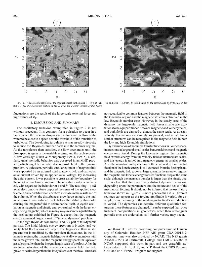
Finally, wemay ask if anything remains visible of any patternenforced by the forcing function FvTG in the higher Reynoldsnumber runs. Figure 12 suggests that the answer is yes. Thisfigure is a plot for run B0 of a cross section ( y ¼ �/4) in whichthe magnetic field strength is exhibited: arrows denote com-ponents in the plane and colors denote components normal tothe plane. The left panel is at t ¼ 70, and the right panel is att ¼ 300. The two horizontal bands are associated with the stag-nation planes of the Taylor-Green forcing.

While at t ¼ 70 the magnetic field is mostly at small scales, att ¼ 300 a pattern reminiscent of the low RV case (Fig. 6d ), albeitmore turbulent, can be clearly seen. This is the result of thesuppression of small scales by the magnetic field. While in thekinematic regime the magnetic field grows under a broad kineticenergy spectrum, when the large-scale magnetic field startsto grow, the small-scale velocity field fluctuations are quenched(Figs. 10 and 11), and the large-scale pattern reappears. This‘‘cleanup’’ effect was also observed in Brandenburg et al. (2001),but there both the large-scale pattern in the flow and the turbulentfluctuations at small scale were imposed, while here the turbulent

Fig. 11.—Transfer of energy in Fourier space in run B0, at (a) t ¼ 13:5 in the kinematic regime (see Fig. 9), (b) t ¼ 73:5 at the end of the kinematic regime,(c) t ¼ 148:5 at the time of rapid growth of the k ¼ 2 shell, and (d ) t ¼ 300. In all the figures, the total transfer at t ¼ 0 (thick solid line) is shown as a reference(which corresponds to the B ¼ 0 case); dotted, dashed, and solid lines represent transfer as indicated in (c). Since TL is negative at most k, �TL is shown. [See theelectronic edition of the Journal for a color version of this figure.]


fluctuations are the result of the large-scale external force andhigh values of RV .

4. DISCUSSION AND SUMMARY

The oscillatory behavior exemplified in Figure 2 is notwithout precedent. It is common for a pulsation to occur in afaucet when the pressure drop is such as to cause the flow of thewater to be close to a speed near the threshold of the transition toturbulence. The developing turbulence acts as an eddy viscosityto reduce the Reynolds number back into the laminar regime.As the turbulence then subsides, the flow accelerates until theflow speed is again in the unstable regime, and the cycle repeats.A few years ago (Shan & Montgomery 1993a, 1993b), a sim-ilarly quasi-periodic behavior was observed in an MHD prob-lem, which might be considered an opposite limit of the dynamoproblem. A quiescent, periodic circular cylinder of magnetofluidwas supported by an external axial magnetic field and carried anaxial current driven by an applied axial voltage. By increasingthe axial current, it was possible to cross a stability boundary forthe onset of mechanical motion. The unstable modes were heli-cal, with regard to the behavior of v and B. The resulting�v<Baxial electromotive force opposed the sense of the applied elec-tric field and constituted an effective increase in the resistance ofthe column. When the disturbances grew large enough, the totalaxial current was reduced back below the stability threshold,causing the magnetofluid to relaminarize itself. A cyclic oscil-lation in magnetic and kinetic energy resulted, with the larger en-ergy beingmagnetic, which inmanyways resembles qualitativelythe oscillations exhibited in Figure 2, except that the magneticenergy remained larger: a sort of ‘‘inverse dynamo’’ problem.

In the high Reynolds case (runs B and B0), part of this dynamicpersists. The initial kinetic energy spectrum is broader, and ve-locity field fluctuations are larger. The large-scale flow is stillpresent but is modified by the turbulent fluctuations. In the ki-nematic regime, themagnetic field grows at all wavenumberswiththe same growth rate, and themagnetic energy spectrum is peakedat scales smaller than the integral length scale of the flow.After thenonlinear saturation of the small-scale magnetic field, the fieldgrows at scales larger than the integral scale of the flow. There are

no recognizable common features between the magnetic field inthe kinematic regime and the magnetic structures observed in thelow Reynolds number case. However, in the steady state of thedynamo, the large-scale magnetic field forces small-scale exci-tations to be equipartitioned betweenmagnetic and velocity fields,and both fields are damped at almost the same scale. As a result,velocity fluctuations are strongly suppressed, and at late timessimilar structures can be recognized in the magnetic field in boththe low and high Reynolds simulations.By examination of nonlinear transfer functions in Fourier space,

interactions at large and small scales between kinetic andmagneticenergy were found. During the kinematic regime, the magneticfield extracts energy from the velocity field at intermediate scales,and this energy is turned into magnetic energy at smaller scales.After the saturation and quenching of the small scales, a substantialfraction of the kinetic energy is still extracted from the forcing band,and themagnetic field grows at large scales. In the saturated regime,the magnetic and kinetic energy transfer functions drop at the samescale, although the magnetic transfer is larger than the kinetic one.It is clear that there are many distinct dynamo behaviors,

depending upon the parameters and the nature and scale of themechanical forcing. It should not be inferred that the oscillatorybehavior shown in Figure 2 is more generic than it is. Differentregimes can appear as the forcing amplitude is varied, for ex-ample, or as the timing of the seed magnetic field’s introductionis varied. The dynamics can acquire different qualitative fea-tures as these features are changed. It can be expected that, onceturbulent computations in geometries other than rectangularperiodic ones are undertaken, still further variety may occur.

We thank H. Tufo for providing computer time at Univer-sity of Colorado, Boulder, NSF ARI grant CDA-9601817.Computer time was also provided by NCAR. The NSF grantsATM-0327533 at Dartmouth College and CMG-0327888 atNCAR supported this work in part and are gratefully ac-knowledged. J. F. P., H. P., and Y. P. thank the CNRS DynamoGdR and INSU/PNST Program for support.

Fig. 12.—Cross-sectional plots of the magnetic field in the plane y ¼ �/4, at (a) t ¼ 70 and (b) t ¼ 300 (Bx, Bz is indicated by the arrows, and By by the color) forrun B0. [See the electronic edition of the Journal for a color version of this figure.]


REFERENCES

Archontis, V., Dorch, S. B. F., & Nordlund, A. 2003, A&A, 410, 759Bourgoin, M., Odier, P., Pinton, J.-F., & Ricard, Y. 2004, Phys. Fluids, 16, 2529Brandenburg, A. 2001, ApJ, 550, 824Brandenburg, A., Bigazzi, A., & Subramanian, K. 2001, MNRAS, 325, 685Haugen, N. E., Brandenburg, A., & Dobler, W. 2004, Phys. Rev. E, 70, 036408Kazantsev, A. P. 1967, Soviet Phys.–JETP, 26, 1031Leorat, J., Pouquet, A., & Frisch, U. 1981, J. Fluid Mech., 104, 419Marie, L., Burguete, J., Daviaud, F., & Leorat, J. 2003, European J. Phys. B,33, 469

Moffatt, H. K. 1978, Magnetic Field Generation in Electrically ConductingFluids (Cambridge: Cambridge Univ. Press)

Morf, R. H., Orszag, S. A., & Frisch, U. 1980, Phys. Rev. Lett., 44, 572Nore, C., Brachet, M. E., Politano, H., & Pouquet, A. 1997, Phys. Plasmas, 4, 1Pelz, R. B., Yakhot, V., Orszag, S. A., Shtilman, L., & Levich, E. 1985, Phys.Rev. Lett., 54, 2505

Ponty, Y., Gilbert, A. D., & Soward, A. M. 2001, in Dynamo and Dynamics: AMathematical Challenge, ed. P. Chossat, D. Armbruster, & I. Oprea (Boston:Kluwer), 261

Ponty, Y., Mininni, P. D., Montgomery, D. C., Pinton, J.-F., Politano, H., &Pouquet, A. 2005, Phys. Rev. Lett., 94, 164502

Pouquet, A., Frisch, U., & Leorat, J. 1976, J. Fluid Mech., 77, 321Taylor, G. I., & Green, A. E. 1937, Proc. R. Soc. London A, 158, 499Schaeffer, N. 2004, Ph.D. thesis, Universite Joseph Fourier (Grenoble)Schekochihin, A. A., Cowley, S. C., Maron, J. L., & McWilliams, J. C. 2004,Phys. Rev. Lett., 92, 054502

Shan, X., & Montgomery, D. 1993a, Plasma Phys. Controlled Fusion, 35, 619———. 1993b, Plasma Phys. Controlled Fusion, 35, 1019Verma, M. K. 2004, Phys. Rep., 401, 229Yousef, T. A., Brandenburg, A., & Rudiger, G. 2003, A&A, 411, 321


dynamo regimes with a nonhelical forcing

Documents