GKSS 99/E/46

Long-wave forcingfor regional atmospheric modelling

Authors:

H. von StorchH. LangenbergF.Feser(Institute of Hydrophysics)

GKSS-Forschungszentrum Geesthacht GmbH • Geesthacht • 1999

0 120 240 360–1

–0.5

0

0.5

1

6 hour intervals

Prop

ortio

n of

repr

esen

ted

varia

nce

GKSS 99/E/46

Long-wave forcing for regional atmospheric modelling

H. von Storch, H. Langenberg, F. Feser

32 pages with 12 figures and 2 tables

Abstract

A new method, named "spectral nudging", of linking a regional model to the driving large-scalemodel simulated or analyzed by a global model is proposed and tested. Spectral nudging isbased on the idea that regional-scale c1imate statistics are conditioned by the interplay betweencontinental-scale atmospheric conditions and such regional features as marginal seas and mountainranges. Following this "downscaling" idea, the regional model is forced to satisfy not onlyboundary conditions, possibly in a boundary sponge region, but also large-scale flow conditionsinside the integration area.

We demonstrate that spectral nudging succeeds in keeping the simulated state elose to the drivingstate at larger scales, while generating smaller-scale features. We also show that the standardboundary forcing technique in current use allows the regional model to develop internal statesconflicting with the large-scale state. It is conc1uded that spectral nudging may be seen as asuboptimal and indirect data assimilation technique.

LangweIliger Antrieb für regionale atmosphärische Modellierung

Zusammenfassung

Eine neue Methode, genannt "spektrales nudging", ein Regionalmodell an das durch ein Global-modell simulierte großskalige Antriebsfeld zu koppeln, wird vorgestellt und getestet. Das spektralenudging basiert auf der Annahme, daß regionale Klimastatistik durch die Wechselwirkung zwischendem kontinental-skaligen atmosphärischen Zustand und regionalen Gegeben-heiten, wie kleinereSeen und Gebirgszüge, bestimmt wird. Demnach muß das Regionalmodell nicht nur die Rand-bedingungen erfüllen, sondern auch die großskaligen Zustände innerhalb des Integrationsgebieteswiedergeben können.

Wir zeigen, daß durch das spektrale nudging der großskalige modellierte Zustand nahe an dem desAntriebsfeldes liegt, ohne die Modellierung regionaler Phänomene zu beeinträchtigen. Außerdemzeigen wir, daß das Regionalmodell durch die zur Zeit benutzte Antriebstechnik über den Modell-rand interne Felder produzieren kann, die zu dem großskaligen Zustand im Widerspruch stehen. Wirschließen daraus, daß das spektrale nudging als eine suboptimale, indirekte Datenassimilierungs-methode angesehen werden kann.

Manuscript received / Manuskripteingang in der Redaktion: 31. August 1999

Contents

1 Background 7

2 REMO model 9

3 Spectral Nudging 11

4 Results 13

4.1 E�ciency of Large-Scale Control . . . . . . . . . . . . . . . . . . . . . . . . . . 13

4.2 Comparison with observational data . . . . . . . . . . . . . . . . . . . . . . . . 22

4.3 Sensitivity experiments . . . . . . . . . . . . . . . . . . . . . . . . . . . . . . . . 26

5 Conclusions 26

6 Acknowledgments 27

7 References 28

-7-

1 Background

The state of the atmosphere can not be observed in its entirety. Only samples of mostly

point observations irregularly distributed in space are available. They are used by operational

weather centers to construct, or \analyze", a continuous distribution of atmospheric variables.

Such \analyses" are our best guess of the atmospheric state and deviate from the true, unknown

state to some extent. Likely, the large scales are best described, simply because they are better

sampled. On the other hand, the details on scales of a few tens of kilometers and less, are

insu�ciently sampled and subject to signi�cant uncertainty.

In old days, the analyses were prepared by hand, and a major achievement of meteorology

was the �nding by the Bergen school at about 1920 that the appearance of the sky contains

information about the state of the atmosphere which should be incorporated into the analysis

and weather forecasting process (Friedmann, 1989). The advent of satellites, with their quasi-

complete mapping of horizontal distributions, has improved the situation considerably. The

major breakthrough was the systematic interpretation of observational data aided by quasi-

realistic dynamical models. However, the only features which can be well reproduced by these

objective analyses with quasi-realistic models are those that are well resolved by the model.

For example, while the e�ect of the Baltic Sea may to some extent be captured, the imprint of

Jutland, separating the Baltic Sea from the North Sea, may not. Thus, the lacking detail in

analyses remains at present a major problem in weather analyses.

While in former days the purpose of weather, or synoptic, analyses was for preparing short-

term weather forecasts, these analyses have in recent years attained a di�erent role, namely to

provide a data base for climatic and other environmental studies. For ful�lling this purpose, it is

no longer su�cient to have the best analysis at a given day. It is also necessary that the quality

of the analyses is homogeneous, so that improvements of the analysis process do not introduce

arti�cial signals in the climate data set. For meeting this requirements, weather services have

prepared so-called global re-analyses, i.e., they have analyzed weather observations of the past

decades with the same analysis scheme (Kalnay et al., 1996).

We suggest a new technique for using these global re-analyses to derive smaller-scale analyses.

-8-

Our technique is based on the view that small scale details are the result of an interplay between

larger-scale atmospheric ow and smaller-scale geographic features such as topography, land-

sea distribution or land-use (von Storch, 1999). To describe this small-scale response, a regional

climate model is forced with large-scale weather analyses. Di�erently from the conventional

approach, the forcing is not only stipulated at the lateral boundaries but also in the interior.

This interior forcing is maintained by adding nudging terms in the spectral domain, with

maximum e�ciency for large scales and no e�ect for small scales. We name the technique

\spectral nudging". Also, the e�ciency is formulated to depend on height and the variable

under consideration. As far as we know this technique is new, but it shares similarities with

methods to force area averages upon the interior solution as proposed by Kida et al. (1991) and

Sasaki et al. (1995). Our method makes use of Giorgi et al.'s (1993) approach who introduce

a height-dependent forcing of their regional model.

For purposes of weather analysis, our proposed technique is suboptimal. Ideally, inside the

model area one would directly assimilate local observational data, which had little impact on

the coarse-grid global re-analyses and, accordingly, were not fully exploited. However, such a

scheme is technically very demanding and often not feasible. The proposed technique may be

considered a \poor woman's data assimilation technique".

The same technique may be used to derive regional scale climate change scenarios from global

climate models (\downscaling"; von Storch, 1995). The basic idea of downscaling is to transfer

onto smaller scales that large-scale information which has been simulated reliably in climate

change scenarios. This is done with the help of statistical models or dynamical regional climate

models. The latter technique, named \dynamical downscaling" uses output from global climate

models to force regional atmospheric (e.g., Giorgi (1990), Jacob and Podzun (1997), Kidson

and Thompson (1998), Rinke and Dethlo� (1999)) or regional oceanic model (Kauker, 1999).

In nearly all studies performed to date, the forcing is administered exclusively at the lateral

boundaries. The technique of statistical dynamical downscaling developed by Fuentes and

Heimann (1996) and Frey-Buness et al. (1995) is related to our approach, as they consider the

response of a regional climate model to prescribed conditions such as the geostrophic wind.

In our view, the conventional practise of using forcing exclusively along the lateral boundaries

-9-

stems from the classic view of regional weather modeling as being a boundary problem rather

than a downscaling problem. Problems like data assimilation and downscaling were not con-

sidered in classical numerical mathematics. The inclusion of the \sponge zone" (Davies, 1976)

was already a violation of the \pure" mathematical concept. In this paper we demonstrate

that the boundary value format is conceptually inappropriate for the problem at hand.

The present paper is organized as follows. A brief introduction of the regional atmospheric

model is given in Section 2. The spectral nudging technique is described in Section 3, and the

results are presented and discussed in Section 4. The discussion makes use of measures, which

quantify the degree of similarity or dissimilarity on di�erent spatial scales. Sensitivity exper-

iments dealing with the strength of the coupling are considered. Conclusions are summarized

in Section 5.

2 REMO model

We use the regional climate model REMO as described by Jacob and Podzun (1997). REMO

is a grid point model featuring the discretized primitive equations in a terrain-following hybrid

coordinates system. Details are given by Jacob and Podzun (1997) and Jacob et al. (1995). The

�nite di�erencing scheme is energy preserving. The prognostic variables are surface pressure,

horizontal wind components, temperature, speci�c humidity and cloud water. A soil model is

added to account for soil temperature and water content.

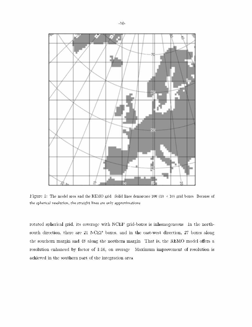
The integration area shown in Figure 1 has a horizontal spherical resolution of 0.5o with a

pole at 170oW; 35oN , resulting in 91 � 81 grid points. Because of the spherical resolution,

the straight grid lines shown in the map are only approximate. A time step of 5 minutes is

adopted.

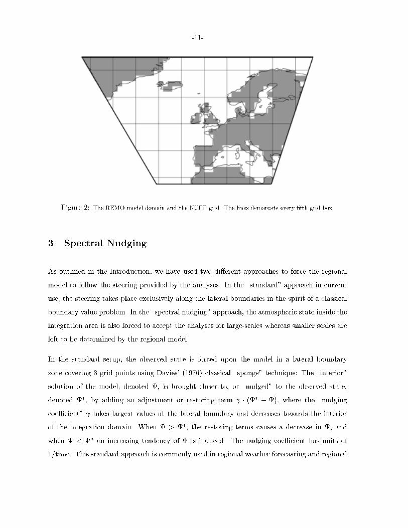
REMO is forced with NCEP re-analyses (Kalnay et al., 1996) over the three month period

of January to March 1993. These observed states are updated every six hours. In between,

values are derived through linear interpolation. The horizontal resolution of the analyses is

approximately 2o longitudinally and latitudinally (Figure 2). Since REMO operates with a

-10-

Figure 1: The model area and the REMO grid. Solid lines demarcate 100 (10 � 10) grid boxes. Because of

the spherical resolution, the straight lines are only approximations.

rotated spherical grid, its coverage with NCEP grid-boxes is inhomogeneous. In the north-

south direction, there are 21 NCEP boxes, and in the east-west direction, 27 boxes along

the southern margin and 48 along the northern margin. That is, the REMO model o�ers a

resolution enhanced by factor of 1:16, on average. Maximum improvement of resolution is

achieved in the southern part of the integration area.

-11-

Figure 2: The REMO model domain and the NCEP grid. The lines demarcate every �fth grid box.

3 Spectral Nudging

As outlined in the Introduction, we have used two di�erent approaches to force the regional

model to follow the steering provided by the analyses. In the \standard" approach in current

use, the steering takes place exclusively along the lateral boundaries in the spirit of a classical

boundary value problem. In the \spectral nudging" approach, the atmospheric state inside the

integration area is also forced to accept the analyses for large-scales whereas smaller scales are

left to be determined by the regional model.

In the standard setup, the observed state is forced upon the model in a lateral boundary

zone covering 8 grid points using Davies' (1976) classical \sponge" technique: The \interior"

solution of the model, denoted , is brought closer to, or \nudged" to the observed state,

denoted �, by adding an adjustment or restoring term � (�� ), where the \nudging

coe�cient" takes largest values at the lateral boundary and decreases towards the interior

of the integration domain. When > �, the restoring terms causes a decrease in , and

when < � an increasing tendency of is induced. The nudging coe�cient has units of

1/time. This standard approach is commonly used in regional weather forecasting and regional

-12-

climate simulations. The \sponge" zone has been introduced to avoid re ection of traveling

features at the boundaries. Any inconsistencies stemming from internally generated features

traveling towards the lateral boundaries and con icting there with the prescribed conditions

are dampened out in this manner.

In the \spectral nudging" approach, the lateral \sponge forcing" is kept and an additional

steering is introduced as described next.

Consider the expansion of a suitable REMO variable:

(�; �; t) =

Jm;KmXj=�Jm;k=�Km

�mj;k(t)eij�=L�eik�=L� (1)

with zonal coordinates �, zonal wave-numbers j and zonal extension of the area L�. Meridional

coordinates are denoted by �, meridional wave-numbers by k, and the meridional extension by

L�. t represents time. For REMO, the number of zonal and meridional wave-numbers is Jm

and Km. A similar expansion is done for the analyses, which are given on a coarser grid. The

coe�cients of this expansion are labeled �aj;k, and the number of Fourier coe�cients is Ja < Jm

and Ka < Km. The con�dence we have in the realism of the di�erent scales of the re-analysis

depends on the wavenumbers j and k and is denoted by �j;k.

The model is then allowed to deviate from the state given by the re-analysis conditional upon

this con�dence. This is achieved by adding \nudging terms" in the spectral domain in both

directionsJa;KaX

j=�Ja;k=�Ka

�j;k(�a

j;k(t)� �mj;k(t))eij�=L�eik�=L� (2)

In the following, we will use the nudging terms dependent on height. That is, our con�dence

in the reanalyses increases with height. On the other hand, we leave the regional model more

room for its own dynamics at the lower levels where we expect regional geographical features

are becoming more important. The better the con�dence, the larger the �j;k-values and the

more e�cient the nudging term.

In this study, we have applied nudging to the zonal and meridional wind components. Following

the prescription of the German Weather Service version of REMO, which uses a pointwise

nudging in case of excessively high wind speeds for preventing numerical instability, we have

-13-

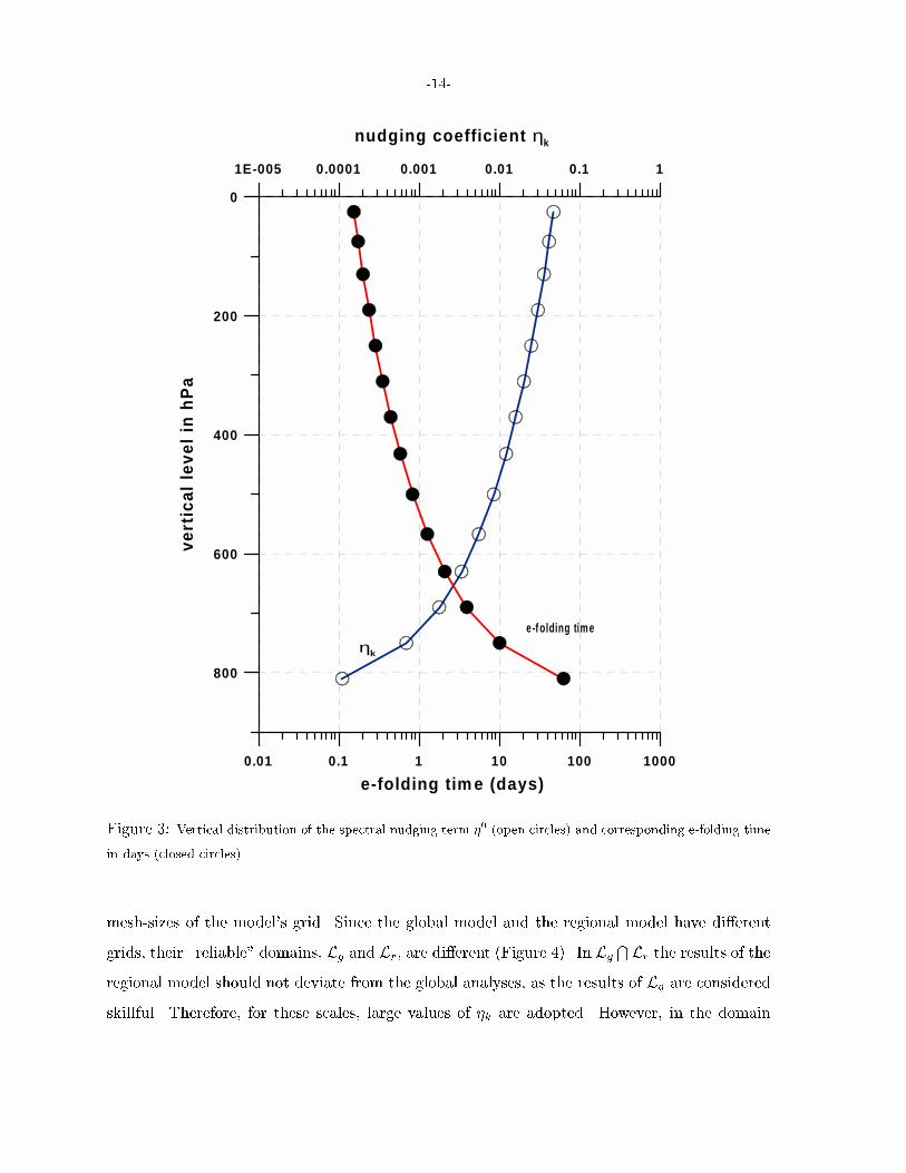
adopted the vertical pro�le

�0(p) =

8><>:

��1� p

850hPa

�2

for p < 850hPa

0 for p > 850hPa(3)

with p denoting pressure (Doms et al., 1995). In our base simulation with spectral nudging we

used the ad-hoc value � = 0:05, resulting in a vertical pro�le as shown in Figure 3. This choice

amounts to an e-folding decay time of an introduced disturbance of about 60 days at 850 hPa,

1 day at 500 hPa and about 3 hours at the model's top level of 25 hPa.

We have set �j;k = �0 for j = 0 : : : 3 in the north-south direction, k = 0 : : : 5 in the east-west

direction and �j;k = 0 otherwise. That is, wavelengths of about 15o and larger are considered to

be reliably analysed by NCEP, corresponding to 6 and more NCEP grid points. More elaborate

speci�cations could certainly have been used. However, some sensitivity experiments indicated

that the e�ect would be somewhat marginal (see below).

4 Results

We demonstrate in Section 4.1 that spectral nudging successfully prevents the regional model

from deviating from the given large-scale state. We also show that signi�cant deviations take

place when the standard approach is used. In Section 4.2, a comparison with station data

reveals that the spectral control is limited to the largest scales, so that the representation of

the local time series is indeed improved compared to the NCEP reanalysis and the REMO

standard run. In Section 4.3, a number of sensitivity experiments is presented and discussed.

4.1 E�ciency of Large-Scale Control

We divide the spectral domain into several intervals. We assume that both the regional and

global model have two spectral domains: a large-scale domain, L and a small-scale domain,

S. The model has di�erent skills in the domains L and S to realistically analyze or simulate

the real state. Only the results in L are considered reliable. So far there is no objective way

to identify the interval L, but it is often believed that the largest wave-number in L is several

-14-

1E-005 0.0001 0.001 0.01 0.1 1

nudging coefficient ηk

800

600

400

200

0ve

rtic

al l

evel

in

hP

a

0.01 0.1 1 10 100 1000

e-folding tim e (days)

ηk

e-f olding time

Figure 3: Vertical distribution of the spectral nudging term �0 (open circles) and corresponding e-folding time

in days (closed circles).

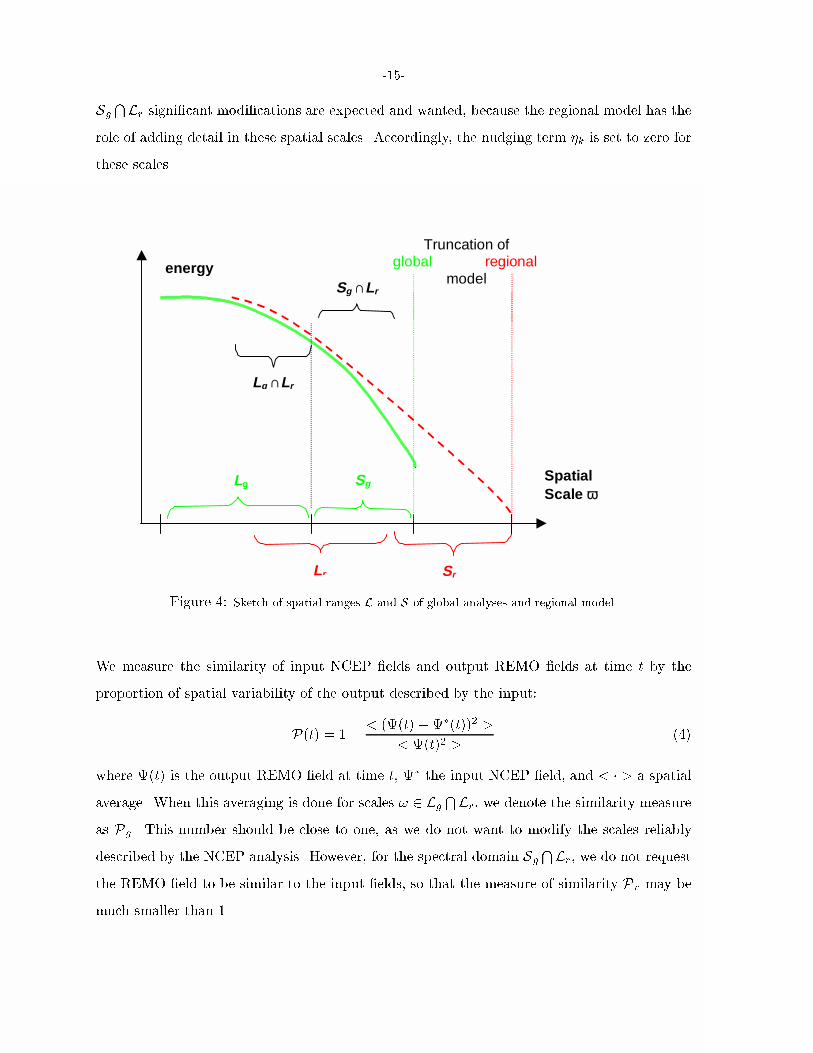
mesh-sizes of the model's grid. Since the global model and the regional model have di�erent

grids, their \reliable" domains, Lg and Lr, are di�erent (Figure 4). In LgTLr the results of the

regional model should not deviate from the global analyses, as the results of Lg are considered

skillful. Therefore, for these scales, large values of �k are adopted. However, in the domain

-15-

Sg

TLr signi�cant modi�cations are expected and wanted, because the regional model has the

role of adding detail in these spatial scales. Accordingly, the nudging term �k is set to zero for

these scales.

Truncation ofglobal regional

modelenergy

SpatialScale ϖ

Lg Sg

Lr Sr

Sg ∩Lr

Lg ∩Lr

Figure 4: Sketch of spatial ranges L and S of global analyses and regional model.

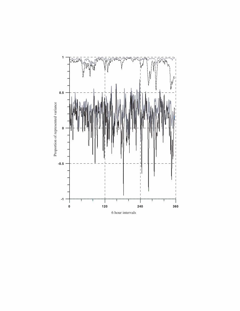
We measure the similarity of input NCEP �elds and output REMO �elds at time t by the

proportion of spatial variability of the output described by the input:

P(t) = 1�< ((t)��(t))2 >

< (t)2 >(4)

where (t) is the output REMO �eld at time t, � the input NCEP �eld, and < � > a spatial

average. When this averaging is done for scales ! 2 LgTLr, we denote the similarity measure

as Pg. This number should be close to one, as we do not want to modify the scales reliably

described by the NCEP analysis. However, for the spectral domain SgTLr, we do not request

the REMO �eld to be similar to the input �elds, so that the measure of similarity Pr may be

much smaller than 1.

-16-

In the present analysis, the set LgTLr is set to comprise zonal wavenumbers up to k � 5 and

meridional wavenumbers j � 3, so that for all (j; k) 2 LgTLr �j;k = �0. The domain Sg

TLr

contains 5 < k � 13 and 3 < j � 10 so that �j;k is zero for these scales . Note that the exact

de�nition of these sets is inconsequential for the performance of the nudging technique as the

numbers Pg and Pr are diagnostics; in fact also the diagnostic results are rather insensitive to

the details of this choice.

The time series of the similarity measures, Pg and Pr, calculated for both the standard run

and for the spectral nudging run, have been calculated for relative humidity and temperature

as well as for the zonal and meridional wind components at 850 and 500 hPa. For the sake of

brevity results are shown only for the meridional wind at 500 hPa in Figure 5.

The desired e�ect of a greater similarity in the spectral range LgTLr is achieved in the spectral

nudging run. In terms of temperature and humidity Pg hardly deviates from the ideal value of 1

in the spectral nudging run (not shown), whereas in the boundary forcing run for the meridional

wind component values less than 1, sometimes as low as 0.6 are obtained (Figure 5). Pr values

between 20% and 40% indicate that REMO considerably modi�es the scales that had been

insu�ciently resolved by NCEP. Pr is mostly somewhat smaller for the standard boundary

forcing run, i.e., controlling the large-scale features in Lgr has some e�ect on SgTLr as well.

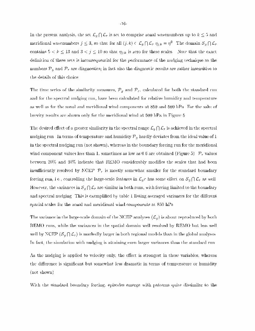
However, the variances in SgTLr are similar in both runs, with forcing limited to the boundary

and spectral nudging. This is exempli�ed by table 1 listing averaged variances for the di�erent

spatial scales for the zonal and meridional wind components at 850 hPa.

The variance in the large-scale domain of the NCEP analyses (Lg) is about reproduced by both

REMO runs, while the variances in the spatial domain well resolved by REMO but less well

well by NCEP (SgTLr) is markedly larger in both regional models than in the global analyses.

In fact, the simulation with nudging is attaining even larger variances than the standard run.

As the nudging is applied to velocity only, the e�ect is strongest in these variables, whereas

the di�erence is signi�cant but somewhat less dramatic in terms of temperature or humidity

(not shown).

With the standard boundary forcing, episodes emerge with patterns quite dissimilar to the

-17-

Table 1:

scale/variable units NCEP REMO REMO

m2s�2 analyses standard nudging

zonal wind

Lg 10�2 1.6 1.2 1.6

Sg

TLr 10�6 3.7 7.7 8.1

meridional wind

Lg 10�2 1.4 1.3 1.5

Sg

TLr 10�6 2.1 6.5 8.5

driving NCEP analysis. An example is the episode of 9-12 March, which is marked by low Pg-

similarity for the zonal wind (Figure 5). In this situation (Figure 6), a persistent high pressure

system is placed in the center of the integration area, blocking the eastward propagation of

synoptic disturbances. For example, the low pressure center initially located over Iceland

moves northeast-ward and the trough west of Ireland moves towards the British Isles and is

dissipated there. In the standard run, this trough is not dissipated as quickly and causes the

central European high to be distorted. In the spectral nudging run, on the other hand, the

overall evolution is similar to that of the NCEP re-analyses, but the details deviate to some

extent.

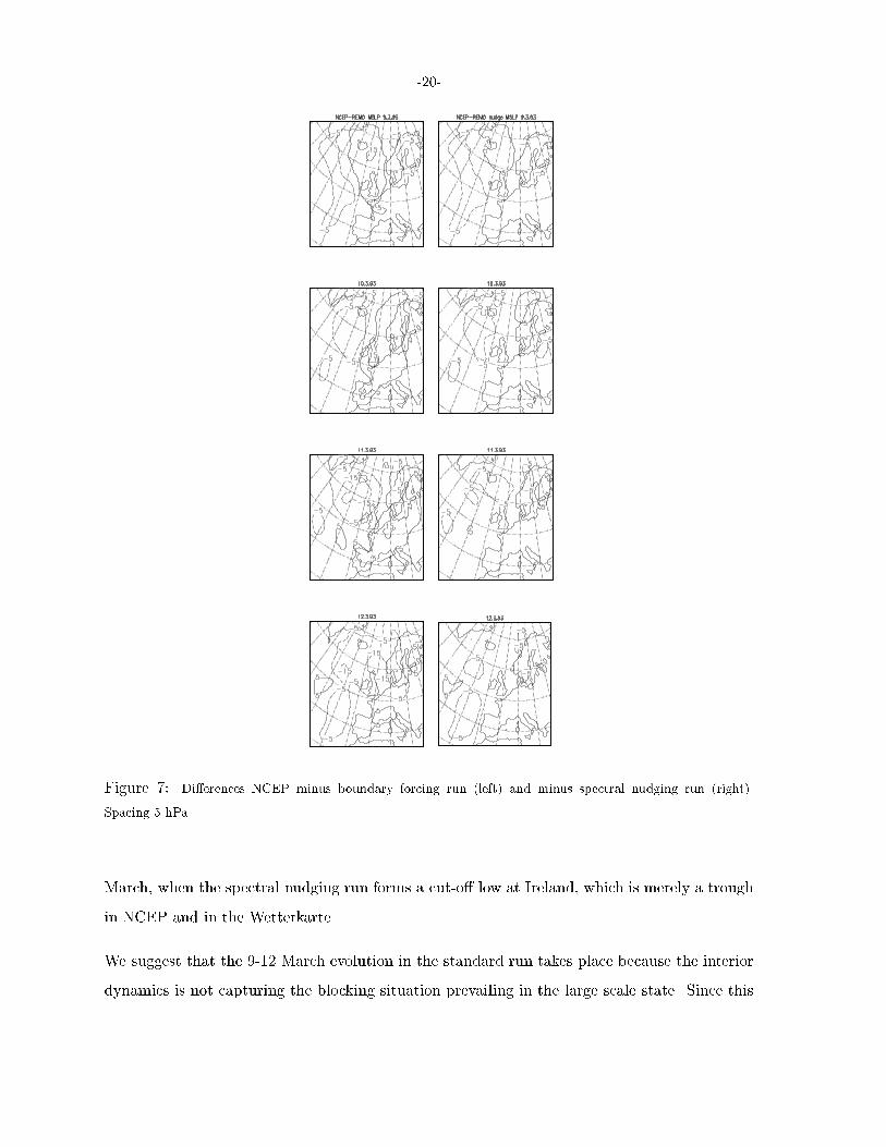
The di�erent evolutions are revealed by the di�erences in the air-pressure distributions of the

boundary forcing run and the NCEP analyses and of the spectral nudging run and NCEP

analysis (Figure 7). Clearly, the air-pressure �eld in the boundary forcing run deviates on

large scales from NCEP. This is particularly striking on 12 March 1993, when over most of

the Atlantic negative air pressure deviations prevail. In the spectral nudging run, on the other

hand, the di�erences arise at a smaller spatial scale. Also the magnitude of the di�erences in

the boundary forcing run, reaching values of 15 hPa and higher in all maps of 9-12 March,

is considerably larger than in the spectral nudging run, where only a few isolated maxima of

about 10 hPa occur.

A comparison with the manually drawn regional analyses of the Berliner Wetterkarte con�rms

0 120 240 360

-1

-0.5

0

0.5

1

6 hour intervals

Prop

ortio

n of

rep

rese

nted

var

ianc

e

-19-

Figure 6: An episode with large di�erences between the standard run and the spectral nudging run: 9-12

March 1993. Surface air pressure distribution. Left column: boundary forcing run; middle: NCEP analyses

(input); right: spectral nudging. Spacing: 5 hPa.

the Berliner Wetterkarte. Also the formation of two separate cyclones over the Atlantic on 12

March is a feature missing in the NCEP re-analyses but identi�ed by the Berlin meteorologists.

On the other hand, sometimes NCEP conforms better with the Wetterkarte; for instance on 9

-20-

Figure 7: Di�erences NCEP minus boundary forcing run (left) and minus spectral nudging run (right).

Spacing 5 hPa.

March, when the spectral nudging run forms a cut-o� low at Ireland, which is merely a trough

in NCEP and in the Wetterkarte.

We suggest that the 9-12 March evolution in the standard run takes place because the interior

dynamics is not capturing the blocking situation prevailing in the large scale state. Since this

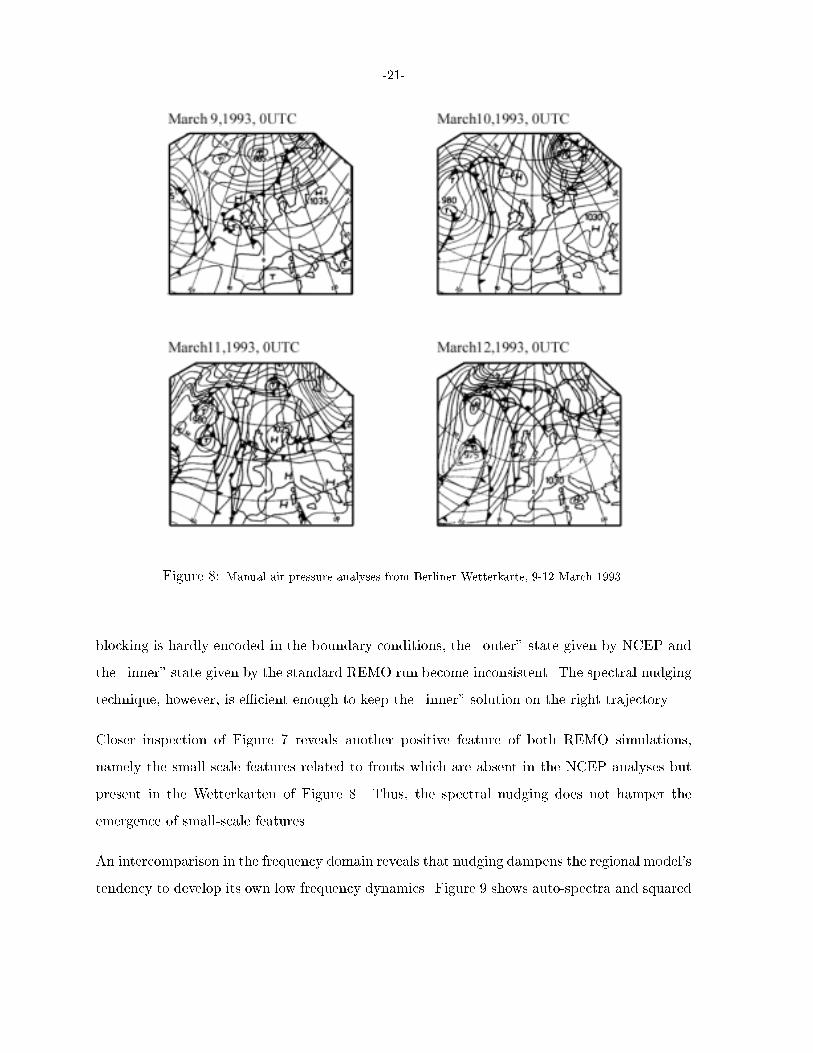
-21-

Figure 8: Manual air pressure analyses from Berliner Wetterkarte, 9-12 March 1993.

blocking is hardly encoded in the boundary conditions, the \outer" state given by NCEP and

the \inner" state given by the standard REMO run become inconsistent. The spectral nudging

technique, however, is e�cient enough to keep the \inner" solution on the right trajectory.

Closer inspection of Figure 7 reveals another positive feature of both REMO simulations,

namely the small scale features related to fronts which are absent in the NCEP analyses but

present in the Wetterkarten of Figure 8. Thus, the spectral nudging does not hamper the

emergence of small-scale features.

An intercomparison in the frequency domain reveals that nudging dampens the regional model's

tendency to develop its own low frequency dynamics. Figure 9 shows auto-spectra and squared

-22-

coherence spectra for air pressure at the station of de Bilt, The Netherlands, for the driving

NCEP analysis (solid) and for the two REMO simulations (dashed). For time periods longer

than about 3 days, the REMO standard run generates additional low frequency variance, which

is suppressed by the nudging. At higher frequencies, both REMO simulations are rather similar.

These �ndings are supported by the squared coherence spectra between the NCEP analyses

and the REMO-simulations; for time periods of 72 hours and more, a much higher coherence

is obtained for the spectral nudging run than for the standard boundary control run, whereas

for shorter time scales, the coherence drops down and the regional model develops its own

dynamics.

4.2 Comparison with observational data

The two REMO runs (with standard boundary forcing and spectral nudging) and the NCEP

re-analyses (only air pressure and temperature) were compared against observed time series

of air pressure, temperature and precipitation at a number of Central European stations. For

the time period January - March 1993, also wind observations from the oil �eld Eko�sk in the

Central North Sea were available; these are compared to the REMO simulations as well (the

NCEP re-analyses have no surface winds)

For air pressure, REMO returns a bias of about 1 hPa for both formulations whereas NCEP

has better mean values (Figure 10). However, the spread of errors is considerably smaller in

the case of the spectral nudging simulation.

For the station of De Bilt in the Netherlands, the cumulative distribution functions of the

di�erence in precipitation between the station data, and the two REMO simulations is shown

in Figure 11. The large step at zero indicates that, in many cases, both models successfully

reproduce dry days. The distributions of positive di�erences \station minus REMO" are equal

in both simulations, but negative di�erences are strongly reduced for the spectral nudging

formulation. For the standard case, the model underestimates the observed precipitation by

up to 40 mm/day whereas in the nudging run these deviations are rarely larger than 20 mm/day.

-23-

60 30

PERIOD [hours]

60 30

PERIOD [hours]

Figure 9: Spectra of analyzed and REMO simulated air pressure at the station De Bilt, The Netherlands.

Top: Auto-spectra: The solid lines refer to the NCEP analyses, the long dashed line to the standard REMO

run, the short dashed line to the spectral nudging REMO run.

Bottom: Squared coherency spectra; the long dashed line refers to the coherence between the NCEP analyses

and the standard run, whereas the shortly dashed line represents the similarity of the spectral nudging run and

the analyses.

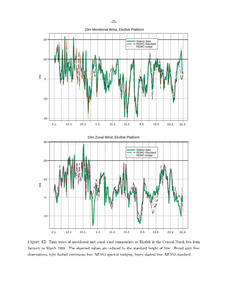
Figure 12 displays time series of the meridional and zonal components of the wind at 10 m height

at Eko�sk in the Central North Sea. Actually, the observations are taken at a higher altitude,

and the values are reduced to a standard height of 10 m through a standard calculation.

-24-

0

2

4

6

-8

-6

-4

-2

De Bilt Frankfurt Geneva Hamburg List Potsdam Uccle ZurichPrague/

LibusPrague/Ruzyn

NCEP REMO Standard REMO Nudge

Figure 10: Di�erences \station data minus simulation" for a series of Central European stations and NCEP,

REMO standard and REMO spectral nudging. The variable considered is air pressure. The di�erences are

displayed as mean plus minus one standard deviation.

All three curves coincide relatively well. A remarkable feature is that in many cases the

maxima and minima of the wind components of the order of 20 m/s are reproduced. A closer

inspection reveals intermittently signi�cant deviations by the standard run and improvements

in the spectral nudging run. The 9-12 March episode emerges clearly in the time series of the

zonal wind.

Figure 11: Cumulative distribution function for the di�erence \de Bilt station data minus simulation" for

REMO nudging, REMO standard and NCEP.

-25-

10m Zonal Wind, Ekofisk Platform

m/s

-10

0

10

20

30

m/s

2.1.

-20

-10

0

10

20

10m Meridional Wind, Ekofisk Platform

12.1 22.1. 1.2. 11.2. 21.2. 3.3. 13.3. 23.3. 31.3.

Station dataREMO StandardREMO nudge

2.1. 12.1 22.1. 1.2. 11.2. 21.2. 3.3. 13.3. 23.3. 31.3.

Station dataREMO StandardREMO nudge

Figure 12: Time series of meridional and zonal wind components at Eko�sk in the Central North Sea from

January to March 1993. The observed values are reduced to the standard height of 10m. Broad grey line:

observations; light dashed continuous line: REMO spectral nudging, heavy dashed line: REMO standard.

-26-

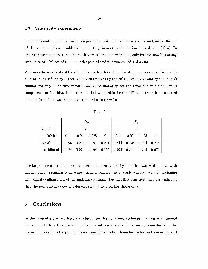
4.3 Sensitivity experiments

Two additional simulations have been performed with di�erent values of the nudging coe�cient

�0. In one run, �0 was doubled (i.e., � = 0:1), in another simulations halved (� = 0:025). In

order to save computer time, the sensitivity experiments were done only for one month, starting

with state of 1 March of the 3-month spectral nudging run considered so far.

We assess the sensitivity of the simulation to this choice by calculating the measures of similarity

Pg and Pr as de�ned by (1) for scales well resolved by the NCEP reanalyses and by the REMO

simulations only. The time mean measures of similarity, for the zonal and meridional wind

components at 500 hPa, is listed in the following table for the di�erent strengths of spectral

nudging (� > 0) as well as for the standard case (� = 0):

Table 2:

Pg Pr

wind � �

at 500 hPa 0.1 0.05 0.025 0 0.1 0.05 0.025 0

zonal 0.996 0.994 0.991 0.931 0.344 0.325 0.304 0.216

meridional 0.984 0.976 0.964 0.855 0.205 0.239 0.205 0.076

The large-scale control seems to be exerted e�ciently also by the other two choices of �, with

markedly higher similiarity measures. A more comprehensive study will be needed for designing

an optimal con�guration of the nudging technique, but this �rst sensitivity analysis indicates

that the performance does not depend signi�cantly on the choice of �.

5 Conclusions

In the present paper we have introduced and tested a new technique to couple a regional

climate model to a time variable global or continental state. This concept deviates from the

classical approach as the problem is not considered to be a boundary value problem in the grid

-27-

point domain, but a downscaling problem. That is, the information which is processed in the

model is not so much the state speci�ed at the areal boundaries but at the large-scales. In a

generalized sense, this is again a boundary problem, but this time formulated in the spectral

domain.

The purpose of the paper was not to delineate the optimal con�guration of spectral nudging, but

to demonstrate the concept, its feasibility and its potential. Our key argument for the success

of the spectral nudging technique is the observations that the nudging technique prevents

the regional model to go astray for limited times, generating internal states inconsistent with

the driving �elds. We have demonstrated that this uncontrolled wandering is not merely a

theoretical problem of the regional model forced from the boundaries, but really takes place.

At the same time, the spectral nudging forcing does not impede the regional model's ability to

develop regional and small scale features superimposed on the large-scale driving conditions.

Di�erent purposes of models require di�erent formulations. When dynamical aspects are to be

addressed, such as the dynamics during the genesis of a storm, the spectral nudging should not

be used, as it modi�es the dynamics inasmuch as it introduces additional forcing terms into

the momentum equation. Also, when a signi�cant two-way-coupling is expected to take place,

as in the case of the life cycle of a hurricane, the spectral nudging will not be adequate. When,

however, speci�cations of regional climate statistics are needed, such as in paleoclimatic and

historic reconstructions and climate change applications, our technique should be preferred as

it generates weather streams consistent with the large-scale driving �elds.

6 Acknowledgments

We are thankful to Daniela Jacob and Ralf Podzun for their help with the model, to Arno

Hellbach for helping us accessing the NCEP data, to Lennart Bengtsson for permission to use

the model, to Mariza Costa-Cabral and Beate M�uller for advice, and to Reiner Schnur for the

observational data. Beate Gardeike professionally prepared many of the diagrams. Ralf Weisse

made the spectral analysis (Figure 9) for us.

-28-

7 References

Davies, H.C., 1976: A lateral boundary formulation for multi-level prediction models. Quart.

J. Roy. Meteor. Soc. 102, 405-418

G. Doms, W. Edelmann, M. Gertz, T. Hanisch, E. Heise, A. Link, D. Majew-

ski, P.Prohl, B. Ritter and U. Schaettler, 1995: Dokumentation des EM/DM-Systems.

Deutscher Wetterdienst Abteilung Forschung, O�enbach a.M.

Frey-Buness, F., D. Heimann and R. Sausen, 1995: A statistical-dynamical downscaling

procedure for global climate simulations. Theor. Appl. Climatol. 50, 117-131

Friedman, R.M., 1989: Appropriating the Weather. Vilhelm Bjerknes and the construction

of a modern meteorology. Cornell University Press, 251 p, ISBN 0 8014-2062-8

Fuentes, U. and D. Heimann, 1996: Veri�cation of statistical-dynamical downscaling in

the Alpine region. Clim. Res. 7:151-186

Giorgi F., 1990: Simulations of regional climate using limited-models nested in a general

circulation model. J. Climate 3, 941-963

Giorgi, F., M.R. Marinucci and G.T Bates, 1993: Development of second-generation

regional climate model (RegCM2). Part II: Convective processes and assimilation of lateral

boundary conditions. Mon. Wea. Rev. 121, 2814-2832

Jacob, D., and R. Podzun, 1997: Sensitivity studies with the regional climate model

REMO. Meteorol. Atmos. Phys. 63, 119-129

Jacob, D., R. Podzun and M. Claussen, 1995: REMO - A model for climate research and

weather prediction. International Workshop on Limited-Area and Variable Resolution Models,

Beijing, China, October 23-27, 1995, 273-278

Kalnay, E., M. Kanamitsu, R. Kistler, W. Collins, D. Deaven, L. Gandin, M.

Iredell, S. Saha, G. White, J. Woollen, Y. Zhu, M. Chelliah, W. Ebisuzaki, W.

Higgins, J. Janowiak, K.C. Mo, C. Ropelewski, J. Wang, A. Leetmaa, R. Reynolds,

R. Jenne, and D. Joseph, 1996: The NCEP/NCAR 40-Year Reanalysis Project. Bull.

Amer. Meteor. Soc. 77, 437-471

Kauker, F., 1998: Regionalization of climate model results for the North Sea. PhD thesis

-29-

University of Hamburg, 109 pp.

Kida, H., T. Koide, H. Sasaki and M. Chiba, 1991: A new approach to coupling a

limited area model with a GCM for regional climate simulation. J. Meteor. Soc. Japan 69,

723-728

Kidson, J.W. and C.S. Thompson, 1998: Comparison of statistical and model-based

downscaling techniques for estimating local climate variations. J. Climate 11, 735-753

Sasaki, H., J. Kida, T. Koide, and M. Chiba, 1995: The performance of long term

integrations of a limited area model with the spectral boundary coupling method. J. Meteor.

Soc. Japan 73, 165-181

von Storch, H., 1995: Inconsistencies at the interface of climate impact studies and global

climate research. Meteorol. Z. 4 NF, 72-80

von Storch, H., 1999: The global and regional climate system. In: H. von Storch and G.

Fl�oser (eds): Anthropogenic Climate Change, Springer Verlag, ISBN 3-540-65033-4, 3-36