ARTICLE IN PRESS

0967-0645/$ - see

doi:10.1016/j.ds

�Correspondifax: +1206 526

E-mail addre

Deep-Sea Research II 54 (2007) 2543–2559

www.elsevier.com/locate/dsr2

Comparison of atmospheric forcing in four sub-arctic seas

Muyin Wanga,�, Nicholas A. Bonda, James E. Overlandb

aJoint Institute for Study of Atmosphere and Ocean, Box 354235, University of Washington, Seattle, Washington 98195, USAbPacific Marine Environmental Laboratory, National Ocean and Atmosphere Administration, 7600 Sand Point Way NE,

Seattle, Washington 98115, USA

Received in revised form 9 August 2007; accepted 21 August 2007

Available online 22 October 2007

Abstract

A comparative analysis was conducted on climate variability in four sub-arctic seas: the Sea of Okhotsk, the Bering Sea

shelf, the Labrador Sea, and the Barents Sea. Based on data from the NCEP/NCAR reanalysis, the focus was on air–sea

interactions, which influence ice cover, ocean currents, mixing, and stratification on sub-seasonal to decadal time scales.

The seasonal cycles of the area-weighted averages of sea-level pressure (SLP), surface air temperature (SAT) and heat

fluxes show remarkable similarity among the four sub-arctic seas. With respect to variation in climate, all four seas

experience changes of comparable magnitude on interannual to interdecadal time scales, but with different timing. Since

2000 warm SAT anomalies were found during most of the year in three of the four sub-arctic seas, with the exception of the

Sea of Okhotsk. A seesaw (out of phase) pattern in winter SAT anomalies between the Labrador and the Barents Sea in the

Atlantic sector is observed during the past 50 years before 2000; a similar type of co-variability between the Sea of Okhotsk

and the Bering Sea shelf in the Pacific is only evident since 1970s. Recent positive anomalies of net heat flux are more

prominent in winter and spring in the Pacific sectors, and in summer in the Atlantic sectors. There is a reduced magnitude

in wind mixing in the Sea of Okhotsk since 1980, in the Barents Sea since 2000, and in early spring/late winter in the Bering

Sea shelf since 1995. Reduced sea-ice areas are seen over three out of four (except the Sea of Okhotsk) sub-arctic seas in

recent decades, particularly after 2000 based on combined in situ and satellite observations (HadISST). This analysis

provides context for the pan-regional synthesis of the linkages between climate and marine ecosystems.

r 2007 Elsevier Ltd. All rights reserved.

Keywords: Atmospheric forcing; Surface heat fluxes; Sea of Okhotsk (44–621N; 135–1601E); Bering Sea shelf (52–661N; 180–1501W);

Labrador Sea (46–691N; 66–431W); Barents Sea (66–811N; 14–661E)

1. Introduction

The four major sub-arctic seas, the Sea ofOkhotsk, the Bering Sea (eastern shelf), the LabradorSea, and the Barents Sea (Fig. 1), support extra-ordinarily rich marine resources, which provide

front matter r 2007 Elsevier Ltd. All rights reserved

r2.2007.08.014

ng author. Tel.: +1206 526 4532;

6485.

ss: muyin.wang@noaa.gov (M. Wang).

food and wealth to regional economies and localcommunities. These sub-arctic seas share severalcommon features: seasonal ice cover, freshwatersources from ice-melt and runoff, pronouncedseasonality in winds and surface heat fluxes, highecosystem abundance, and low biodiversity (Huntand Drinkwater, 2005). Having similar sub-arcticlocations, they represent transition zones between theinfluences of cold, dry air masses of arctic or conti-nental origin and maritime air masses originating

.

ARTICLE IN PRESS

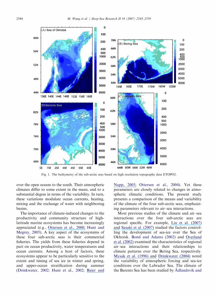
Fig. 1. The bathymetry of the sub-arctic seas based on high resolution topography data ETOPO2.

M. Wang et al. / Deep-Sea Research II 54 (2007) 2543–25592544

over the open oceans to the south. Their atmosphericclimates differ to some extent in the mean, and to asubstantial degree in terms of the variability. In turn,these variations modulate ocean currents, heating,mixing and the exchange of water with neighboringbasins.

The importance of climate-induced changes to theproductivity and community structure of high-latitude marine ecosystems has become increasinglyappreciated (e.g., Ottersen et al., 2000; Hunt andMegrey, 2005). A key aspect of the ecosystems ofthese four sub-arctic seas is their commercialfisheries. The yields from these fisheries depend inpart on ocean productivity, water temperatures andocean currents. Among a host of factors, theseecosystems appear to be particularly sensitive to theextent and timing of sea ice in winter and spring,and upper-ocean stratification during summer(Drinkwater, 2002; Hunt et al., 2002; Baier and

Napp, 2003; Ottersen et al., 2004). Yet theseparameters are closely related to changes in atmo-spheric climatic conditions. The present studypresents a comparison of the means and variabilityof the climate of the four sub-arctic seas, emphasiz-ing parameters relevant to air–sea interactions.

Most previous studies of the climate and air–seainteractions over the four sub-arctic seas areregional specific. For example, Liu et al. (2007)and Sasaki et al. (2007) studied the factors control-ling the development of sea-ice over the Sea ofOkhotsk. Bond and Adams (2002) and Overlandet al. (2002) examined the characteristics of regionalair–sea interactions and their relationships toclimate patterns over the Bering Sea, respectively.Mysak et al. (1996) and Drinkwater (2004) notedthe variability of atmospheric forcing and sea-iceconditions over the Labrador Sea. The climate ofthe Barents Sea has been studied by Adlandsvik and

ARTICLE IN PRESS

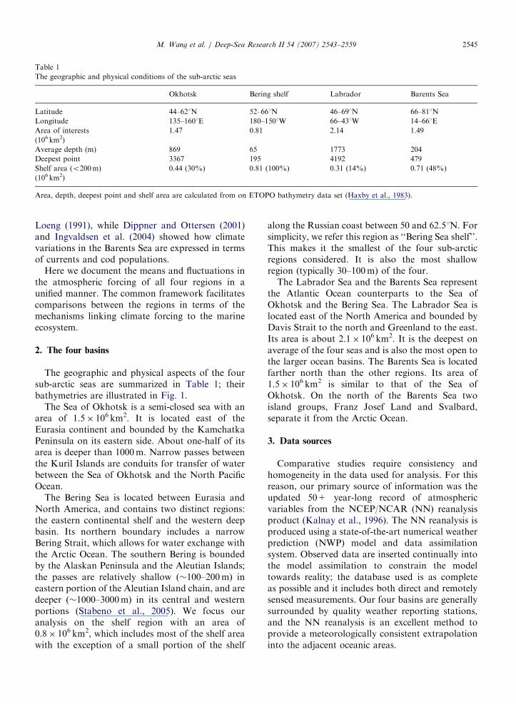
Table 1

The geographic and physical conditions of the sub-arctic seas

Okhotsk Bering shelf Labrador Barents Sea

Latitude 44–621N 52–661N 46–691N 66–811N

Longitude 135–1601E 180–1501W 66–431W 14–661E

Area of interests 1.47 0.81 2.14 1.49

(106 km2)

Average depth (m) 869 65 1773 204

Deepest point 3367 195 4192 479

Shelf area (o200m) 0.44 (30%) 0.81 (100%) 0.31 (14%) 0.71 (48%)

(106 km2)

Area, depth, deepest point and shelf area are calculated from on ETOPO bathymetry data set (Haxby et al., 1983).

M. Wang et al. / Deep-Sea Research II 54 (2007) 2543–2559 2545

Loeng (1991), while Dippner and Ottersen (2001)and Ingvaldsen et al. (2004) showed how climatevariations in the Barents Sea are expressed in termsof currents and cod populations.

Here we document the means and fluctuations inthe atmospheric forcing of all four regions in aunified manner. The common framework facilitatescomparisons between the regions in terms of themechanisms linking climate forcing to the marineecosystem.

2. The four basins

The geographic and physical aspects of the foursub-arctic seas are summarized in Table 1; theirbathymetries are illustrated in Fig. 1.

The Sea of Okhotsk is a semi-closed sea with anarea of 1.5� 106 km2. It is located east of theEurasia continent and bounded by the KamchatkaPeninsula on its eastern side. About one-half of itsarea is deeper than 1000m. Narrow passes betweenthe Kuril Islands are conduits for transfer of waterbetween the Sea of Okhotsk and the North PacificOcean.

The Bering Sea is located between Eurasia andNorth America, and contains two distinct regions:the eastern continental shelf and the western deepbasin. Its northern boundary includes a narrowBering Strait, which allows for water exchange withthe Arctic Ocean. The southern Bering is boundedby the Alaskan Peninsula and the Aleutian Islands;the passes are relatively shallow (�100–200m) ineastern portion of the Aleutian Island chain, and aredeeper (�1000–3000m) in its central and westernportions (Stabeno et al., 2005). We focus ouranalysis on the shelf region with an area of0.8� 106 km2, which includes most of the shelf areawith the exception of a small portion of the shelf

along the Russian coast between 50 and 62.51N. Forsimplicity, we refer this region as ‘‘Bering Sea shelf’’.This makes it the smallest of the four sub-arcticregions considered. It is also the most shallowregion (typically 30–100m) of the four.

The Labrador Sea and the Barents Sea representthe Atlantic Ocean counterparts to the Sea ofOkhotsk and the Bering Sea. The Labrador Sea islocated east of the North America and bounded byDavis Strait to the north and Greenland to the east.Its area is about 2.1� 106 km2. It is the deepest onaverage of the four seas and is also the most open tothe larger ocean basins. The Barents Sea is locatedfarther north than the other regions. Its area of1.5� 106 km2 is similar to that of the Sea ofOkhotsk. On the north of the Barents Sea twoisland groups, Franz Josef Land and Svalbard,separate it from the Arctic Ocean.

3. Data sources

Comparative studies require consistency andhomogeneity in the data used for analysis. For thisreason, our primary source of information was theupdated 50+ year-long record of atmosphericvariables from the NCEP/NCAR (NN) reanalysisproduct (Kalnay et al., 1996). The NN reanalysis isproduced using a state-of-the-art numerical weatherprediction (NWP) model and data assimilationsystem. Observed data are inserted continually intothe model assimilation to constrain the modeltowards reality; the database used is as completeas possible and it includes both direct and remotelysensed measurements. Our four basins are generallysurrounded by quality weather reporting stations,and the NN reanalysis is an excellent method toprovide a meteorologically consistent extrapolationinto the adjacent oceanic areas.

ARTICLE IN PRESS

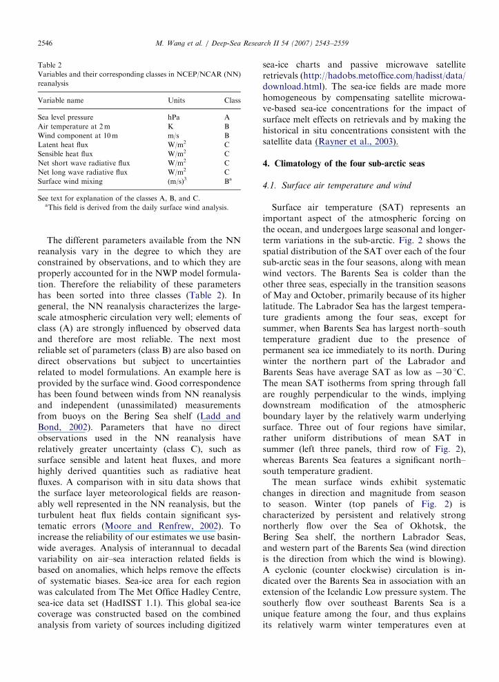
Table 2

Variables and their corresponding classes in NCEP/NCAR (NN)

reanalysis

Variable name Units Class

Sea level pressure hPa A

Air temperature at 2m K B

Wind component at 10m m/s B

Latent heat flux W/m2 C

Sensible heat flux W/m2 C

Net short wave radiative flux W/m2 C

Net long wave radiative flux W/m2 C

Surface wind mixing (m/s)3 Ba

See text for explanation of the classes A, B, and C.aThis field is derived from the daily surface wind analysis.

M. Wang et al. / Deep-Sea Research II 54 (2007) 2543–25592546

The different parameters available from the NNreanalysis vary in the degree to which they areconstrained by observations, and to which they areproperly accounted for in the NWP model formula-tion. Therefore the reliability of these parametershas been sorted into three classes (Table 2). Ingeneral, the NN reanalysis characterizes the large-scale atmospheric circulation very well; elements ofclass (A) are strongly influenced by observed dataand therefore are most reliable. The next mostreliable set of parameters (class B) are also based ondirect observations but subject to uncertaintiesrelated to model formulations. An example here isprovided by the surface wind. Good correspondencehas been found between winds from NN reanalysisand independent (unassimilated) measurementsfrom buoys on the Bering Sea shelf (Ladd andBond, 2002). Parameters that have no directobservations used in the NN reanalysis haverelatively greater uncertainty (class C), such assurface sensible and latent heat fluxes, and morehighly derived quantities such as radiative heatfluxes. A comparison with in situ data shows thatthe surface layer meteorological fields are reason-ably well represented in the NN reanalysis, but theturbulent heat flux fields contain significant sys-tematic errors (Moore and Renfrew, 2002). Toincrease the reliability of our estimates we use basin-wide averages. Analysis of interannual to decadalvariability on air–sea interaction related fields isbased on anomalies, which helps remove the effectsof systematic biases. Sea-ice area for each regionwas calculated from The Met Office Hadley Centre,sea-ice data set (HadISST 1.1). This global sea-icecoverage was constructed based on the combinedanalysis from variety of sources including digitized

sea-ice charts and passive microwave satelliteretrievals (http://hadobs.metoffice.com/hadisst/data/download.html). The sea-ice fields are made morehomogeneous by compensating satellite microwa-ve-based sea-ice concentrations for the impact ofsurface melt effects on retrievals and by making thehistorical in situ concentrations consistent with thesatellite data (Rayner et al., 2003).

4. Climatology of the four sub-arctic seas

4.1. Surface air temperature and wind

Surface air temperature (SAT) represents animportant aspect of the atmospheric forcing onthe ocean, and undergoes large seasonal and longer-term variations in the sub-arctic. Fig. 2 shows thespatial distribution of the SAT over each of the foursub-arctic seas in the four seasons, along with meanwind vectors. The Barents Sea is colder than theother three seas, especially in the transition seasonsof May and October, primarily because of its higherlatitude. The Labrador Sea has the largest tempera-ture gradients among the four seas, except forsummer, when Barents Sea has largest north–southtemperature gradient due to the presence ofpermanent sea ice immediately to its north. Duringwinter the northern part of the Labrador andBarents Seas have average SAT as low as �30 1C.The mean SAT isotherms from spring through fallare roughly perpendicular to the winds, implyingdownstream modification of the atmosphericboundary layer by the relatively warm underlyingsurface. Three out of four regions have similar,rather uniform distributions of mean SAT insummer (left three panels, third row of Fig. 2),whereas Barents Sea features a significant north–south temperature gradient.

The mean surface winds exhibit systematicchanges in direction and magnitude from seasonto season. Winter (top panels of Fig. 2) ischaracterized by persistent and relatively strongnortherly flow over the Sea of Okhotsk, theBering Sea shelf, the northern Labrador Seas,and western part of the Barents Sea (wind directionis the direction from which the wind is blowing).A cyclonic (counter clockwise) circulation is in-dicated over the Barents Sea in association with anextension of the Icelandic Low pressure system. Thesoutherly flow over southeast Barents Sea is aunique feature among the four, and thus explainsits relatively warm winter temperatures even at

ARTICLE IN PRESS

Fig. 2. The climatology of surface air-temperature (shaded), sea-level pressure (SLP) (contour) and surface wind (vectors) for selected

month over each of the sub-arctic seas. The climatology is defined as the 50-year (1951–2000) mean based on NN reanalysis. Contour

interval is 2 hPa for SLP. From left to right it is for the Sea of Okhotsk, the Bering Sea shelf, the Labrador Sea, and the Barents Sea. From

top down, it is for Winter (January), Spring (May), Summer (August), and Autumn (October). The shaded area also indicates the mask of

each sub-arctic sea used in area-weighted averages.

M. Wang et al. / Deep-Sea Research II 54 (2007) 2543–2559 2547

latitudes 10–151 farther north than the other seas.Spring features weaker northerly winds, especiallyin the Sea of Okhotsk. Relatively uniform northerlywinds occur in spring in the Barents Sea (right panelof second row of Fig. 2). In summer, mean windstend to be light, with prevailing southerlies orsouthwesterlies in their southern parts (third row ofFig. 2). By fall, wind patterns resemble those ofwinter, especially in the northern portions of thefour seas (bottom panels of Fig. 2).

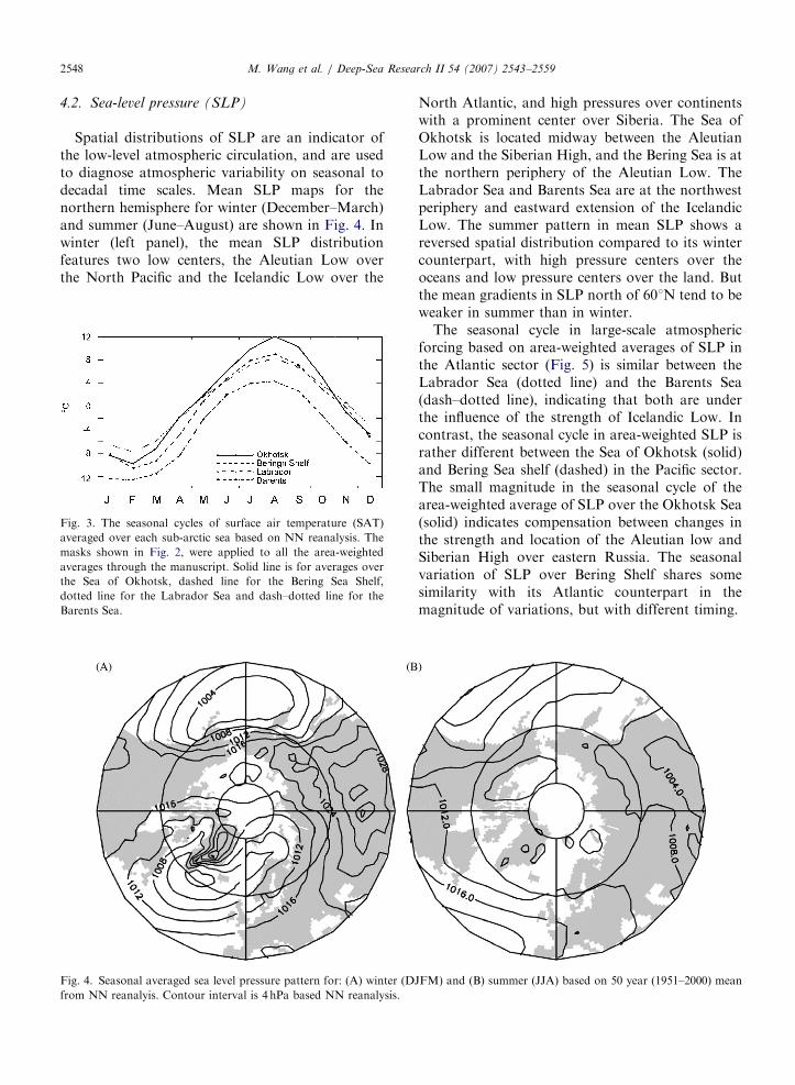
The annual cycle of area-weighted averages ofSAT is shown in Fig. 3, which displays similar

structure among the four sub-arctic seas. That is,they all have maximum temperature in August andminimum temperature in February. The BarentsSea (dash–dotted line) is the coldest of the four seasthroughout the year, and has the smallest variationsin the temperature range. The Sea of Okhotsk (solidline) is the warmest region from spring through fall,and also undergoes the largest seasonal variation.The similar seasonal variations among the fourindicate a close connection of the four sub-arcticseas in association with the change of the hemi-spheric general atmospheric circulations.

ARTICLE IN PRESSM. Wang et al. / Deep-Sea Research II 54 (2007) 2543–25592548

4.2. Sea-level pressure (SLP)

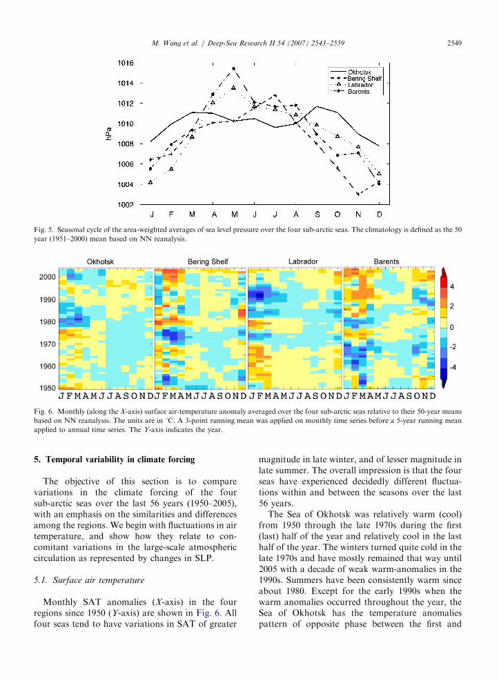
Spatial distributions of SLP are an indicator ofthe low-level atmospheric circulation, and are usedto diagnose atmospheric variability on seasonal todecadal time scales. Mean SLP maps for thenorthern hemisphere for winter (December–March)and summer (June–August) are shown in Fig. 4. Inwinter (left panel), the mean SLP distributionfeatures two low centers, the Aleutian Low overthe North Pacific and the Icelandic Low over the

Fig. 3. The seasonal cycles of surface air temperature (SAT)

averaged over each sub-arctic sea based on NN reanalysis. The

masks shown in Fig. 2, were applied to all the area-weighted

averages through the manuscript. Solid line is for averages over

the Sea of Okhotsk, dashed line for the Bering Sea Shelf,

dotted line for the Labrador Sea and dash–dotted line for the

Barents Sea.

Fig. 4. Seasonal averaged sea level pressure pattern for: (A) winter (D

from NN reanalyis. Contour interval is 4 hPa based NN reanalysis.

North Atlantic, and high pressures over continentswith a prominent center over Siberia. The Sea ofOkhotsk is located midway between the AleutianLow and the Siberian High, and the Bering Sea is atthe northern periphery of the Aleutian Low. TheLabrador Sea and Barents Sea are at the northwestperiphery and eastward extension of the IcelandicLow. The summer pattern in mean SLP shows areversed spatial distribution compared to its wintercounterpart, with high pressure centers over theoceans and low pressure centers over the land. Butthe mean gradients in SLP north of 601N tend to beweaker in summer than in winter.

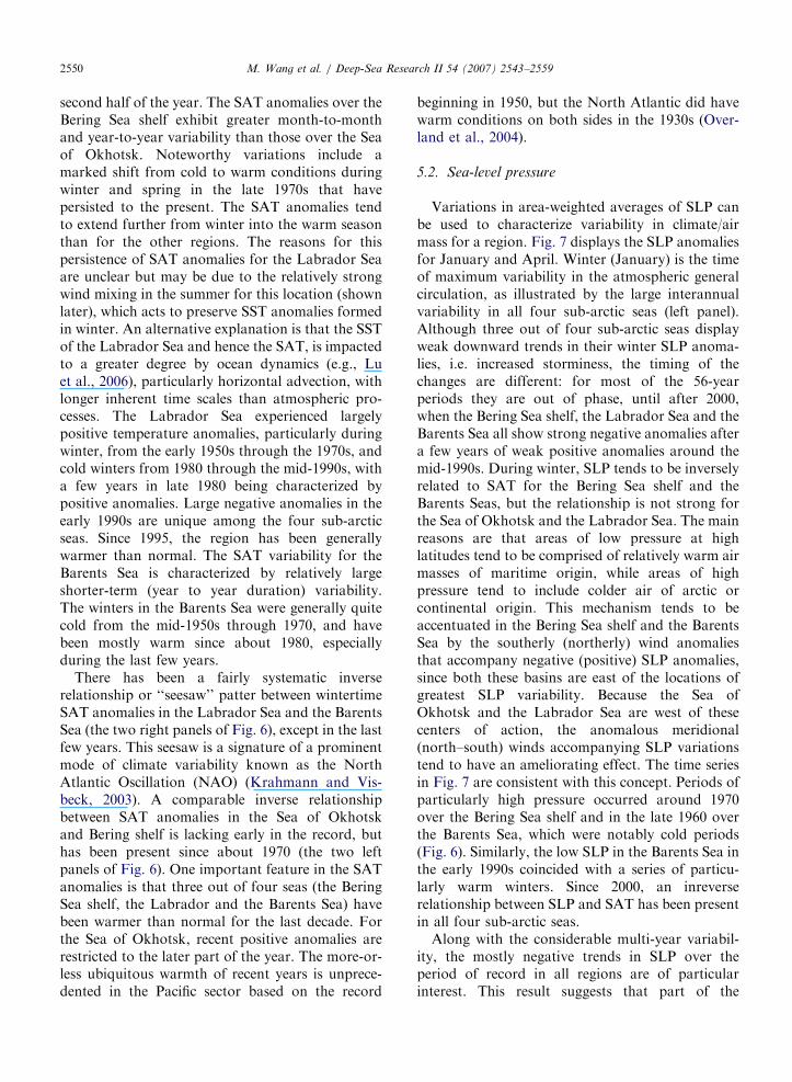
The seasonal cycle in large-scale atmosphericforcing based on area-weighted averages of SLP inthe Atlantic sector (Fig. 5) is similar between theLabrador Sea (dotted line) and the Barents Sea(dash–dotted line), indicating that both are underthe influence of the strength of Icelandic Low. Incontrast, the seasonal cycle in area-weighted SLP israther different between the Sea of Okhotsk (solid)and Bering Sea shelf (dashed) in the Pacific sector.The small magnitude in the seasonal cycle of thearea-weighted average of SLP over the Okhotsk Sea(solid) indicates compensation between changes inthe strength and location of the Aleutian low andSiberian High over eastern Russia. The seasonalvariation of SLP over Bering Shelf shares somesimilarity with its Atlantic counterpart in themagnitude of variations, but with different timing.

JFM) and (B) summer (JJA) based on 50 year (1951–2000) mean

ARTICLE IN PRESS

Fig. 5. Seasonal cycle of the area-weighted averages of sea level pressure over the four sub-arctic seas. The climatology is defined as the 50

year (1951–2000) mean based on NN reanalysis.

Fig. 6. Monthly (along the X-axis) surface air-temperature anomaly averaged over the four sub-arctic seas relative to their 50-year means

based on NN reanalysis. The units are in 1C. A 3-point running mean was applied on monthly time series before a 5-year running mean

applied to annual time series. The Y-axis indicates the year.

M. Wang et al. / Deep-Sea Research II 54 (2007) 2543–2559 2549

5. Temporal variability in climate forcing

The objective of this section is to comparevariations in the climate forcing of the foursub-arctic seas over the last 56 years (1950–2005),with an emphasis on the similarities and differencesamong the regions. We begin with fluctuations in airtemperature, and show how they relate to con-comitant variations in the large-scale atmosphericcirculation as represented by changes in SLP.

5.1. Surface air temperature

Monthly SAT anomalies (X-axis) in the fourregions since 1950 (Y-axis) are shown in Fig. 6. Allfour seas tend to have variations in SAT of greater

magnitude in late winter, and of lesser magnitude inlate summer. The overall impression is that the fourseas have experienced decidedly different fluctua-tions within and between the seasons over the last56 years.

The Sea of Okhotsk was relatively warm (cool)from 1950 through the late 1970s during the first(last) half of the year and relatively cool in the lasthalf of the year. The winters turned quite cold in thelate 1970s and have mostly remained that way until2005 with a decade of weak warm-anomalies in the1990s. Summers have been consistently warm sinceabout 1980. Except for the early 1990s when thewarm anomalies occurred throughout the year, theSea of Okhotsk has the temperature anomaliespattern of opposite phase between the first and

ARTICLE IN PRESSM. Wang et al. / Deep-Sea Research II 54 (2007) 2543–25592550

second half of the year. The SAT anomalies over theBering Sea shelf exhibit greater month-to-monthand year-to-year variability than those over the Seaof Okhotsk. Noteworthy variations include amarked shift from cold to warm conditions duringwinter and spring in the late 1970s that havepersisted to the present. The SAT anomalies tendto extend further from winter into the warm seasonthan for the other regions. The reasons for thispersistence of SAT anomalies for the Labrador Seaare unclear but may be due to the relatively strongwind mixing in the summer for this location (shownlater), which acts to preserve SST anomalies formedin winter. An alternative explanation is that the SSTof the Labrador Sea and hence the SAT, is impactedto a greater degree by ocean dynamics (e.g., Luet al., 2006), particularly horizontal advection, withlonger inherent time scales than atmospheric pro-cesses. The Labrador Sea experienced largelypositive temperature anomalies, particularly duringwinter, from the early 1950s through the 1970s, andcold winters from 1980 through the mid-1990s, witha few years in late 1980 being characterized bypositive anomalies. Large negative anomalies in theearly 1990s are unique among the four sub-arcticseas. Since 1995, the region has been generallywarmer than normal. The SAT variability for theBarents Sea is characterized by relatively largeshorter-term (year to year duration) variability.The winters in the Barents Sea were generally quitecold from the mid-1950s through 1970, and havebeen mostly warm since about 1980, especiallyduring the last few years.

There has been a fairly systematic inverserelationship or ‘‘seesaw’’ patter between wintertimeSAT anomalies in the Labrador Sea and the BarentsSea (the two right panels of Fig. 6), except in the lastfew years. This seesaw is a signature of a prominentmode of climate variability known as the NorthAtlantic Oscillation (NAO) (Krahmann and Vis-beck, 2003). A comparable inverse relationshipbetween SAT anomalies in the Sea of Okhotskand Bering shelf is lacking early in the record, buthas been present since about 1970 (the two leftpanels of Fig. 6). One important feature in the SATanomalies is that three out of four seas (the BeringSea shelf, the Labrador and the Barents Sea) havebeen warmer than normal for the last decade. Forthe Sea of Okhotsk, recent positive anomalies arerestricted to the later part of the year. The more-or-less ubiquitous warmth of recent years is unprece-dented in the Pacific sector based on the record

beginning in 1950, but the North Atlantic did havewarm conditions on both sides in the 1930s (Over-land et al., 2004).

5.2. Sea-level pressure

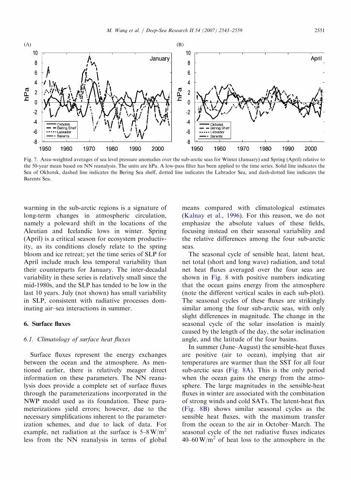
Variations in area-weighted averages of SLP canbe used to characterize variability in climate/airmass for a region. Fig. 7 displays the SLP anomaliesfor January and April. Winter (January) is the timeof maximum variability in the atmospheric generalcirculation, as illustrated by the large interannualvariability in all four sub-arctic seas (left panel).Although three out of four sub-arctic seas displayweak downward trends in their winter SLP anoma-lies, i.e. increased storminess, the timing of thechanges are different: for most of the 56-yearperiods they are out of phase, until after 2000,when the Bering Sea shelf, the Labrador Sea and theBarents Sea all show strong negative anomalies aftera few years of weak positive anomalies around themid-1990s. During winter, SLP tends to be inverselyrelated to SAT for the Bering Sea shelf and theBarents Seas, but the relationship is not strong forthe Sea of Okhotsk and the Labrador Sea. The mainreasons are that areas of low pressure at highlatitudes tend to be comprised of relatively warm airmasses of maritime origin, while areas of highpressure tend to include colder air of arctic orcontinental origin. This mechanism tends to beaccentuated in the Bering Sea shelf and the BarentsSea by the southerly (northerly) wind anomaliesthat accompany negative (positive) SLP anomalies,since both these basins are east of the locations ofgreatest SLP variability. Because the Sea ofOkhotsk and the Labrador Sea are west of thesecenters of action, the anomalous meridional(north–south) winds accompanying SLP variationstend to have an ameliorating effect. The time seriesin Fig. 7 are consistent with this concept. Periods ofparticularly high pressure occurred around 1970over the Bering Sea shelf and in the late 1960 overthe Barents Sea, which were notably cold periods(Fig. 6). Similarly, the low SLP in the Barents Sea inthe early 1990s coincided with a series of particu-larly warm winters. Since 2000, an inreverserelationship between SLP and SAT has been presentin all four sub-arctic seas.

Along with the considerable multi-year variabil-ity, the mostly negative trends in SLP over theperiod of record in all regions are of particularinterest. This result suggests that part of the

ARTICLE IN PRESS

Fig. 7. Area-weighted averages of sea level pressure anomalies over the sub-arctic seas for Winter (January) and Spring (April) relative to

the 50-year mean based on NN reanalysis. The units are hPa. A low-pass filter has been applied to the time series. Solid line indicates the

Sea of Okhotsk, dashed line indicates the Bering Sea shelf, dotted line indicates the Labrador Sea, and dash-dotted line indicates the

Barents Sea.

M. Wang et al. / Deep-Sea Research II 54 (2007) 2543–2559 2551

warming in the sub-arctic regions is a signature oflong-term changes in atmospheric circulation,namely a poleward shift in the locations of theAleutian and Icelandic lows in winter. Spring(April) is a critical season for ecosystem productiv-ity, as its conditions closely relate to the springbloom and ice retreat; yet the time series of SLP forApril include much less temporal variability thantheir counterparts for January. The inter-decadalvariability in these series is relatively small since themid-1980s, and the SLP has tended to be low in thelast 10 years. July (not shown) has small variabilityin SLP, consistent with radiative processes dom-inating air–sea interactions in summer.

6. Surface fluxes

6.1. Climatology of surface heat fluxes

Surface fluxes represent the energy exchangesbetween the ocean and the atmosphere. As men-tioned earlier, there is relatively meager directinformation on these parameters. The NN reana-lysis does provide a complete set of surface fluxesthrough the parameterizations incorporated in theNWP model used as its foundation. These para-meterizations yield errors; however, due to thenecessary simplifications inherent to the parameter-ization schemes, and due to lack of data. Forexample, net radiation at the surface is 5–8W/m2

less from the NN reanalysis in terms of global

means compared with climatological estimates(Kalnay et al., 1996). For this reason, we do notemphasize the absolute values of these fields,focusing instead on their seasonal variability andthe relative differences among the four sub-arcticseas.

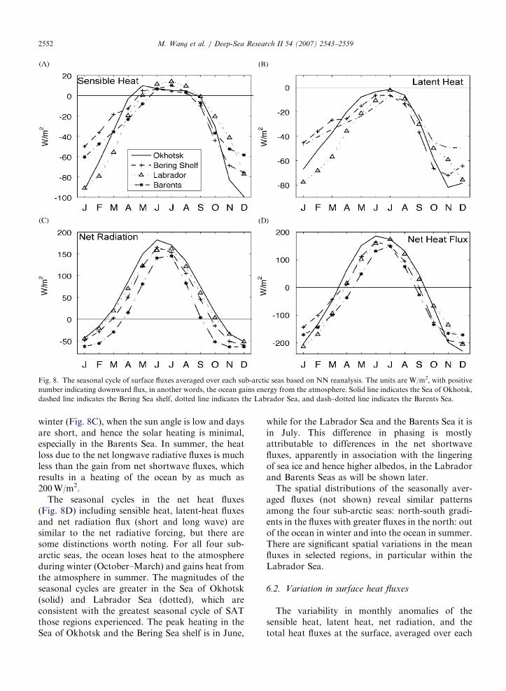
The seasonal cycle of sensible heat, latent heat,net total (short and long wave) radiation, and totalnet heat fluxes averaged over the four seas areshown in Fig. 8 with positive numbers indicatingthat the ocean gains energy from the atmosphere(note the different vertical scales in each sub-plot).The seasonal cycles of these fluxes are strikinglysimilar among the four sub-arctic seas, with onlyslight differences in magnitude. The change in theseasonal cycle of the solar insolation is mainlycaused by the length of the day, the solar inclinationangle, and the latitude of the four basins.

In summer (June–August) the sensible-heat fluxesare positive (air to ocean), implying that airtemperatures are warmer than the SST for all foursub-arctic seas (Fig. 8A). This is the only periodwhen the ocean gains the energy from the atmo-sphere. The large magnitudes in the sensible-heatfluxes in winter are associated with the combinationof strong winds and cold SATs. The latent-heat flux(Fig. 8B) shows similar seasonal cycles as thesensible heat fluxes, with the maximum transferfrom the ocean to the air in October–March. Theseasonal cycle of the net radiative fluxes indicates40–60W/m2 of heat loss to the atmosphere in the

ARTICLE IN PRESS

Fig. 8. The seasonal cycle of surface fluxes averaged over each sub-arctic seas based on NN reanalysis. The units are W/m2, with positive

number indicating downward flux, in another words, the ocean gains energy from the atmosphere. Solid line indicates the Sea of Okhotsk,

dashed line indicates the Bering Sea shelf, dotted line indicates the Labrador Sea, and dash–dotted line indicates the Barents Sea.

M. Wang et al. / Deep-Sea Research II 54 (2007) 2543–25592552

winter (Fig. 8C), when the sun angle is low and daysare short, and hence the solar heating is minimal,especially in the Barents Sea. In summer, the heatloss due to the net longwave radiative fluxes is muchless than the gain from net shortwave fluxes, whichresults in a heating of the ocean by as much as200W/m2.

The seasonal cycles in the net heat fluxes(Fig. 8D) including sensible heat, latent-heat fluxesand net radiation flux (short and long wave) aresimilar to the net radiative forcing, but there aresome distinctions worth noting. For all four sub-arctic seas, the ocean loses heat to the atmosphereduring winter (October–March) and gains heat fromthe atmosphere in summer. The magnitudes of theseasonal cycles are greater in the Sea of Okhotsk(solid) and Labrador Sea (dotted), which areconsistent with the greatest seasonal cycle of SATthose regions experienced. The peak heating in theSea of Okhotsk and the Bering Sea shelf is in June,

while for the Labrador Sea and the Barents Sea it isin July. This difference in phasing is mostlyattributable to differences in the net shortwavefluxes, apparently in association with the lingeringof sea ice and hence higher albedos, in the Labradorand Barents Seas as will be shown later.

The spatial distributions of the seasonally aver-aged fluxes (not shown) reveal similar patternsamong the four sub-arctic seas: north-south gradi-ents in the fluxes with greater fluxes in the north: outof the ocean in winter and into the ocean in summer.There are significant spatial variations in the meanfluxes in selected regions, in particular within theLabrador Sea.

6.2. Variation in surface heat fluxes

The variability in monthly anomalies of thesensible heat, latent heat, net radiation, and thetotal heat fluxes at the surface, averaged over each

ARTICLE IN PRESSM. Wang et al. / Deep-Sea Research II 54 (2007) 2543–2559 2553

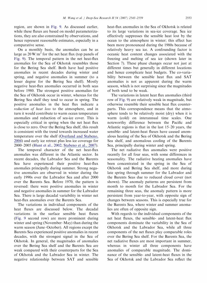
region, are shown in Fig. 9. As discussed earlier,while these fluxes are based on model parameteriza-tions, they are also constrained by observations, andhence represent reasonable estimates, especially in acomparative sense.

On a monthly basis, the anomalies can be aslarge as 20W/m2 for the net heat flux (top panels ofFig. 9). The temporal pattern in the net heat-fluxanomalies for the Sea of Okhotsk resembles thosefor the Bering Sea shelf. Both have had positiveanomalies in recent decades during winter andspring, and negative anomalies in summer (to alesser degree for the Bering Sea shelf). Mostlynegative heat-flux anomalies occurred in both seasbefore 1980. The strongest positive anomalies forthe Sea of Okhotsk occur in winter, whereas for theBering Sea shelf they tend to occur in spring. Thepositive anomalies in the heat flux indicate areduction of heat loss to the atmosphere, and inturn it would contribute to warm ocean temperatureanomalies and reduction of sea-ice cover. This isespecially critical in spring when the net heat fluxis close to zero. Over the Bering Sea shelf, this resultis consistent with the trend towards increased watertemperature over the shelf (Overland and Stabeno,2004) and early ice retreat plus less ice coverage for2000–2005 (Hunt et al., 2002; Stabeno et al., 2007).

The temporal character of the net heat-fluxanomalies was different in the Atlantic sector. Inrecent decades, the Labrador Sea and the BarentsSea have experienced their positive heat-fluxanomalies principally during summer. Strong nega-tive anomalies are observed in winter during theearly 1990s over the Labrador Sea and after 2000over the Barents Sea. Before 1970, the pattern isreversed: there were positive anomalies in winterand negative anomalies in summer for the LabradorSea. There is large decadal variability in winter netheat-flux anomalies over the Barents Sea.

The variations in individual components of theheat fluxes are discussed below. The decadalvariations in the surface sensible heat fluxes(Fig. 9 second row) are more prominent duringwinter and spring (November–May) than during thewarm season (June–October). All regions except theBarents Sea experienced positive anomalies in recentdecades, with the strongest signal in the Sea ofOkhotsk. In general, the magnitudes of anomaliesover the Bering Sea shelf and the Barents Sea areweak compared with their counterparts for the Seaof Okhotsk and the Labrador Sea in winter. Thenegative relationship between SAT and sensible

heat-flux anomalies in the Sea of Okhotsk is relatedto its large variations in sea-ice coverage. Sea iceeffectively suppresses the sensible heat lost by theocean to the atmosphere in winter; this effect hasbeen more pronounced during the 1980s because ofrelatively heavy sea ice. A confounding factor isoceanic heat content changes associated with thefreezing and melting of sea ice (shown later inSection 7). These phase changes occur not just atdifferent times but generally in different locationsand hence complicate heat budgets. The co-varia-bility between the sensible heat flux and SATanomalies is not as apparent during the warmseason, which is not surprising since the magnitudesof both tend to be weak.

The variations in latent heat flux anomalies (thirdrow of Fig. 9) are relatively weak in magnitude, butotherwise resemble their sensible heat flux counter-parts. This correspondence means that the atmo-sphere tends to be relatively moist (dry) when it iswarm (cold) on interannual time scales. Onenoteworthy difference between the Pacific andAtlantic regions is that in the last 15–20 years, thesensible- and latent-heat fluxes have caused anom-alous heating of the Sea of Okhotsk and the BeringSea shelf, and anomalous cooling of the BarentsSea, principally during winter and spring.

The net radiative flux anomalies were positiverecently for all four seas, with some differences inseasonality. The radiative heating anomalies havebeen concentrated in the spring in the Sea ofOkhotsk and Bering Sea shelf, and more duringlate spring through summer for the Labrador andthe Barents Seas due to reduced cloud cover (notshown). The anomaly patterns are persistent frommonth to month for the Labrador Sea. For theremaining three seas, the anomaly pattern is morepersistent from year-to-year, with opposite sign ofchanges between seasons. This is especially true forthe Barents Sea, where winter and summer anoma-lies are often of opposite sign.

With regards to the individual components of thenet heat fluxes, the sensible- and latent-heat fluxcomponents dominate the variability in the Sea ofOkhotsk and the Labrador Sea, while all threecomponents of the net fluxes play comparable rolesover the Bering Sea shelf. For the Barents Sea, thenet radiative fluxes are most important in summer,whereas in winter all three components haveanomalies of comparable magnitude. The domi-nance of the sensible- and latent-heat fluxes in theSea of Okhotsk and the Labrador Sea reflect the

ARTICLE IN PRESS

Fig. 9. Monthly surface heat flux anomalies averaged over the four sub-arctic seas based on NN reanalysis. From top down it is for net

heat fluxes, sensible heat, latent heat, and net radiative flux. The units are in W/m2, and positive numbers (warm colors) indicating

downward fluxes. From left to right the panels are for the Sea of Okhotsk, the Bering Sea shelf, the Labrador Sea and the Barents Sea.

A 3-point running mean was applied on monthly time series before a 5-year running mean applied to the annual time series for each

individual month.

M. Wang et al. / Deep-Sea Research II 54 (2007) 2543–25592554

ARTICLE IN PRESSM. Wang et al. / Deep-Sea Research II 54 (2007) 2543–2559 2555

prevalence of cold, dry air masses of continentalorigin relative to the Bering Sea shelf and theBarents Sea.

While there have been periods of significantlynegative net heat-flux anomalies in the last twodecades in all four regions, these anomalies havelacked persistence from season to season. Theretended to be less seasonality to the net coolingevents before the 1980s. While our analysis pre-cludes differentiating cause from effect, previouswork indicates that it is the atmosphere that largelycontrols the variability in air–sea interactions overthe North Pacific and North Atlantic (Kushniret al., 2002).

6.3. Climatology and variations of wind mixing

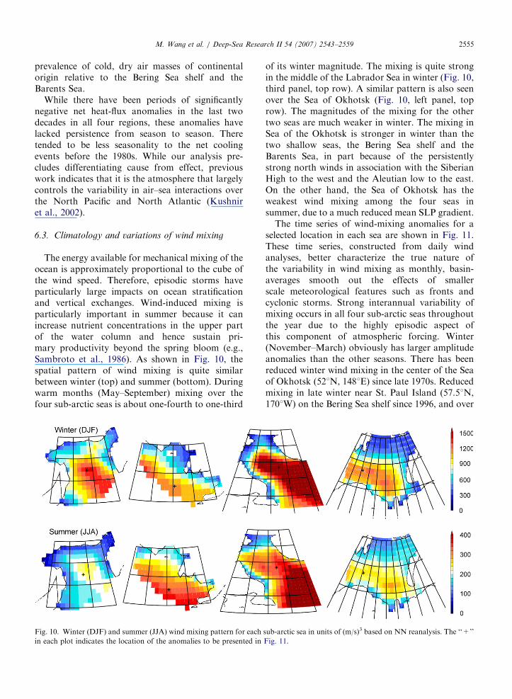
The energy available for mechanical mixing of theocean is approximately proportional to the cube ofthe wind speed. Therefore, episodic storms haveparticularly large impacts on ocean stratificationand vertical exchanges. Wind-induced mixing isparticularly important in summer because it canincrease nutrient concentrations in the upper partof the water column and hence sustain pri-mary productivity beyond the spring bloom (e.g.,Sambroto et al., 1986). As shown in Fig. 10, thespatial pattern of wind mixing is quite similarbetween winter (top) and summer (bottom). Duringwarm months (May–September) mixing over thefour sub-arctic seas is about one-fourth to one-third

Fig. 10. Winter (DJF) and summer (JJA) wind mixing pattern for each

in each plot indicates the location of the anomalies to be presented in

of its winter magnitude. The mixing is quite strongin the middle of the Labrador Sea in winter (Fig. 10,third panel, top row). A similar pattern is also seenover the Sea of Okhotsk (Fig. 10, left panel, toprow). The magnitudes of the mixing for the othertwo seas are much weaker in winter. The mixing inSea of the Okhotsk is stronger in winter than thetwo shallow seas, the Bering Sea shelf and theBarents Sea, in part because of the persistentlystrong north winds in association with the SiberianHigh to the west and the Aleutian low to the east.On the other hand, the Sea of Okhotsk has theweakest wind mixing among the four seas insummer, due to a much reduced mean SLP gradient.

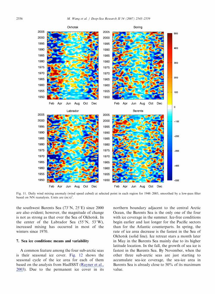
The time series of wind-mixing anomalies for aselected location in each sea are shown in Fig. 11.These time series, constructed from daily windanalyses, better characterize the true nature ofthe variability in wind mixing as monthly, basin-averages smooth out the effects of smallerscale meteorological features such as fronts andcyclonic storms. Strong interannual variability ofmixing occurs in all four sub-arctic seas throughoutthe year due to the highly episodic aspect ofthis component of atmospheric forcing. Winter(November–March) obviously has larger amplitudeanomalies than the other seasons. There has beenreduced winter wind mixing in the center of the Seaof Okhotsk (521N, 1481E) since late 1970s. Reducedmixing in late winter near St. Paul Island (57.51N,1701W) on the Bering Sea shelf since 1996, and over

sub-arctic sea in units of (m/s)3 based on NN reanalysis. The ‘‘+’’

Fig. 11.

ARTICLE IN PRESS

Fig. 11. Daily wind mixing anomaly (wind speed cubed) at selected point in each region for 1948–2005, smoothed by a low-pass filter

based on NN reanalysis. Units are (m/s)3.

M. Wang et al. / Deep-Sea Research II 54 (2007) 2543–25592556

the southwest Barents Sea (731N, 251E) since 2000are also evident; however, the magnitude of changeis not as strong as that over the Sea of Okhotsk. Inthe center of the Labrador Sea (551N, 531W),increased mixing has occurred in most of thewinters since 1970.

7. Sea ice conditions: means and variability

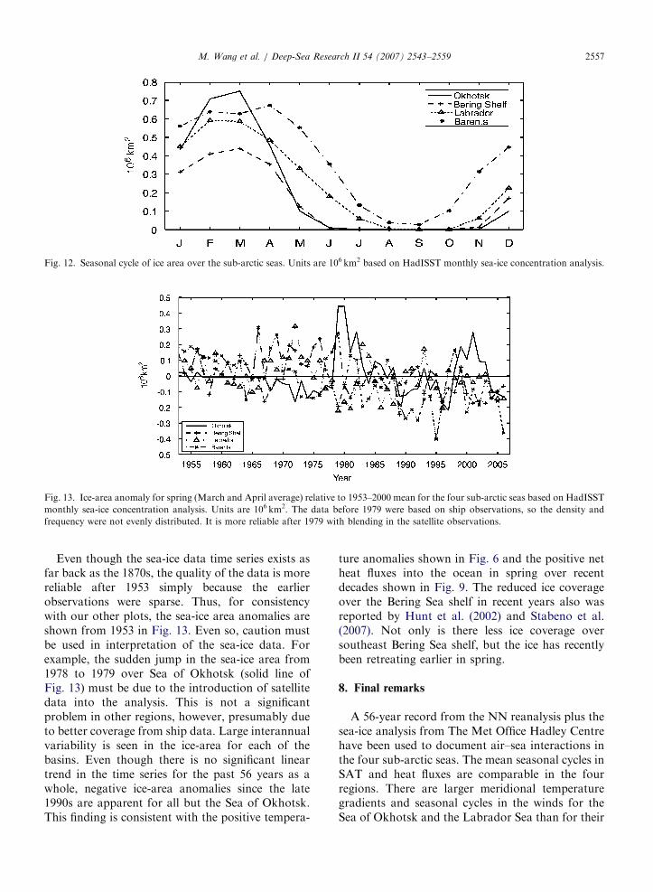
A common feature among the four sub-arctic seasis their seasonal ice cover. Fig. 12 shows theseasonal cycle of the ice area for each of thembased on the analysis from HadISST (Rayner et al.,2003). Due to the permanent ice cover in its

northern boundary adjacent to the central ArcticOcean, the Barents Sea is the only one of the fourwith ice coverage in the summer. Ice-free conditionsbegin earlier and last longer for the Pacific sectorsthan for the Atlantic counterparts. In spring, therate of ice area decrease is the fastest in the Sea ofOkhotsk (solid line). Ice retreat stars a month laterin May in the Barents Sea mainly due to its higherlatitude location. In the fall, the growth of sea ice isfastest in the Barents Sea. By November, when theother three sub-arctic seas are just starting toaccumulate sea-ice coverage, the sea-ice area inBarents Sea is already close to 50% of its maximumvalue.

ARTICLE IN PRESS

Fig. 12. Seasonal cycle of ice area over the sub-arctic seas. Units are 106 km2 based on HadISST monthly sea-ice concentration analysis.

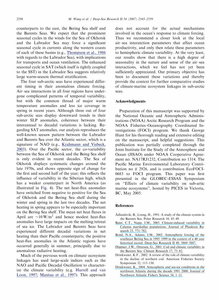
Fig. 13. Ice-area anomaly for spring (March and April average) relative to 1953–2000 mean for the four sub-arctic seas based on HadISST

monthly sea-ice concentration analysis. Units are 106 km2. The data before 1979 were based on ship observations, so the density and

frequency were not evenly distributed. It is more reliable after 1979 with blending in the satellite observations.

M. Wang et al. / Deep-Sea Research II 54 (2007) 2543–2559 2557

Even though the sea-ice data time series exists asfar back as the 1870s, the quality of the data is morereliable after 1953 simply because the earlierobservations were sparse. Thus, for consistencywith our other plots, the sea-ice area anomalies areshown from 1953 in Fig. 13. Even so, caution mustbe used in interpretation of the sea-ice data. Forexample, the sudden jump in the sea-ice area from1978 to 1979 over Sea of Okhotsk (solid line ofFig. 13) must be due to the introduction of satellitedata into the analysis. This is not a significantproblem in other regions, however, presumably dueto better coverage from ship data. Large interannualvariability is seen in the ice-area for each of thebasins. Even though there is no significant lineartrend in the time series for the past 56 years as awhole, negative ice-area anomalies since the late1990s are apparent for all but the Sea of Okhotsk.This finding is consistent with the positive tempera-

ture anomalies shown in Fig. 6 and the positive netheat fluxes into the ocean in spring over recentdecades shown in Fig. 9. The reduced ice coverageover the Bering Sea shelf in recent years also wasreported by Hunt et al. (2002) and Stabeno et al.(2007). Not only is there less ice coverage oversoutheast Bering Sea shelf, but the ice has recentlybeen retreating earlier in spring.

8. Final remarks

A 56-year record from the NN reanalysis plus thesea-ice analysis from The Met Office Hadley Centrehave been used to document air–sea interactions inthe four sub-arctic seas. The mean seasonal cycles inSAT and heat fluxes are comparable in the fourregions. There are larger meridional temperaturegradients and seasonal cycles in the winds for theSea of Okhotsk and the Labrador Sea than for their

ARTICLE IN PRESSM. Wang et al. / Deep-Sea Research II 54 (2007) 2543–25592558

counterparts to the east, the Bering Sea shelf andthe Barents Seas. We expect that the prominentseasonal cycles in the winds for the Sea of Okhotskand the Labrador Sea may force a significantseasonal cycle in currents along the western coastsof each of these basins (e.g., Thompson et al., 1986with regards to the Labrador Sea), with implicationsfor transports and ocean ventilation. The enhancedseasonal cycle in SAT (which itself is tightly coupledto the SST) in the Labrador Sea suggests relativelylarge warm-season thermal stratification.

The four sub-arctic seas have experienced differ-ent timing in their anomalous climate forcing.Air–sea interactions in all four regions have under-gone complicated patterns of temporal variability,but with the common thread of major warmtemperature anomalies and less ice coverage inspring in recent years. Although three out of foursub-arctic seas display downward trends in theirwinter SLP anomalies, coherence between theirinterannual to decadal variations is lacking. Re-garding SAT anomalies, our analysis reproduces thewell-known seesaw pattern between the Labradorand Barents Sea over the Atlantic sector, which is asignature of NAO (e.g., Krahmann and Visbeck,2003). Over the Pacific sector, the co-variabilitybetween the Sea of Okhotsk and the Being Sea shelfis only evident in recent decades. The Sea ofOkhotsk displays systematic changes around thelate 1970s, and shows opposite sign of change forthe first and second half of the year; this reflects theinfluence of variability in the Siberian high, whichhas a weaker counterpart in North America (asillustrated in Fig. 4). The net heat-flux anomalieshave switched from negative to positive for the Seaof Okhotsk and the Bering Sea shelf during thewinter and spring in the last two decades. The netheating in spring appears to be especially importanton the Bering Sea shelf. The mean net heat fluxes inApril are �10W/m2 and hence modest heat-fluxanomalies have large impacts on the melting/retreatof sea ice. The Labrador and Barents Seas haveexperienced different decadal variations in netheating than their Pacific counterparts; the positiveheat-flux anomalies in the Atlantic regions haveoccurred generally in summer, principally due toanomalous radiative heating.

Much of the previous work on climate–ecosystemlinkages has used large-scale indices such as theNAO and Pacific Decadal Oscillation to character-ize the climate variability (e.g. Hurrell and vanLoon, 1997; Mantua et al., 1997). This approach

does not account for the actual mechanismsinvolved in the ocean’s response to climate forcing.Thus we recommend a closer look at the localair–sea interatction parameters that affect oceanproductivity, and only then relate these parametersto hemispheric climate variability. At the very least,our results show that there is a high degree ofseasonality in the nature and sense of the air–seainteractions, which we feel has not yet beensufficiently appreciated. Our primary objective hasbeen to document these variations and therebyprovide the context for further comparative studiesof climate-marine ecosystem linkages in sub-arcticseas.

Acknowledgments

Preparation of this manuscript was supported bythe National Oceanic and Atmospheric Adminis-trations (NOAA) Arctic Research Program and theNOAA Fisheries–Oceanography Coordinated In-vestigations (FOCI) program. We thank GeorgeHunt for his thorough reading and extensive editingon the manuscript, and helpful suggestions. Thispublication was partially completed through theJoint Institute for the Study of the Atmosphere andOcean (JISAO) under NOAA Cooperative Agree-ment no. NA17RJ1232, Contribution no 1314. ThePacific Marine Environmental Laboratory Contri-bution no # 2926, and is contribution EcoFOCI-0683 to FOCI program. This paper was firstpresented in the GLOBEC-ESSAS Symposiumon ‘‘Effects of climate variability on sub-articmarine ecosystems’’, hosted by PICES in Victoria,BC, May 2005.

References

Adlandsvik, B., Loeng, H., 1991. A study of the climate system in

the Barents Sea. Polar Research 10, 45–49.

Baier, C.T., Napp, J.M., 2003. Climate-induced variability in

Calanus marshallae populations. Journal of Plankton Re-

search 25, 771–782.

Bond, N.A., Adams, J.M., 2002. Atmospheric forcing of the

southeast Bering Sea in 1995–1999 in the context of a 40 year

historical record. Deep-Sea Research II 49, 5869–5887.

Dippner, J.W., Ottersen, G., 2001. Cod and climate variability in

the Barents Sea. Climate Research 17, 73–82.

Drinkwater, K.F., 2002. A review of the role of climate variability

in the decline of northern cod. American Fisheries Society

Symposium 32, 113–130.

Drinkwater, K., 2004. Atmospheric and sea-ice conditions in the

northwest Atlantic during the decade 1991–2000. Journal of

Northwest Atlantic Fishery Science 34, 1–11.

ARTICLE IN PRESSM. Wang et al. / Deep-Sea Research II 54 (2007) 2543–2559 2559

Haxby, W.F., Labrecque, J.L., Weissel, J.K., Karner, G.D., 1983.

Digital images of combined oceanic and continental data sets

and their use in tectonic studies. EOS Transactions of the

American Physical Union 64 (52), 995–1004.

Hunt Jr., G.L., Drinkwater, K. (Eds.), 2005. Background on the

climatology, physical oceanography and ecosystems of the

sub-arctic seas: Appendix to the ESSAS Science Plan.

GLOBEC Report No. 20, viii, 96pp.

Hunt Jr., G.L., Stabeno, P., Walters, G., Sinclair, E., Brodeur,

R.D., Napp, J.M., Bond, N.A., 2002. Climate change and

control of the southeastern Bering Sea pelagic ecosystem.

Deep-Sea Research II 49, 5821–5853.

Hunt Jr., G.L., Megrey, B.A., 2005. Comparison of the

biophysical and trophic characteristics of the Bering and

Barents Seas. ICES Journal of Marine Science 62, 1245–1255.

Hurrell, J.W., van Loon, H., 1997. Decadal variations in climate

associated with the North Atlantic oscillation. Climatic

Change 36, 301–326.

Ingvaldsen, R., Asplin, L., Loeng, H., 2004. The seasonal cycle in

the Atlantic transport to the Barents Sea during the years

1997–2001. Continental Shelf Research 24, 1015–1032.

Kalnay, E., Kanamitsu, M., Kistler, R., Collins, W., Deaven, D.,

Gandin, L., Iredell, M., Saha, S., White, G., Woollen, J., Zhu,

Y., Chelliah, M., Ebisuzaki, W., Higgins, W., Janowiak, J.,

Mo, K.C., Ropelewski, C., Wang, J., Leetmaa, A., Reynolds,

R., Jenne, R., Joseph, D., 1996. The NCEP/NCAR 40-year

reanalysis project. Bulletin of the American Meteorological

Society 77, 437–471.

Krahmann, G., Visbeck, M., 2003. Variability in Northern

Annular Mode’s signature in winter sea Ice concentration.

Polar Research 21, 51–57.

Kushnir, Y., Robinson, W.A., Blade, I., Hall, N.M.J., Peng, S.,

Sutton, R., 2002. Atmospheric GCM response to extratropi-

cal SST anomalies: synthesis and evaluation. Journal of

Climate 15, 2233–2256.

Ladd, C., Bond, N.A., 2002. Evaluation of the NCEP-NCAR

Reanalysis in the northeast Pacific and the Bering Sea.

Journal of Geophysical Research 107, 3158.

Liu, J.P., Zhang, Z., Horton, R.M., Wang, C., Ren, X., 2007.

Variability of North Pacific sea ice and East Asia-North

Pacific winter climate. Journal of Climate 20, 1991–2001.

Lu, Y., Wright, D.G., Clarke, R.A., 2006. Modelling deep

seasonal temperature changes in the Labrador Sea. Geophy-

sics Research Letter 33, L23601.

Mantua, N.J., Hare, S.R., Zhang, Y., Wallace, J.M., Francis,

R.C., 1997. A Pacific interdecadal climate oscillation with

impacts on salmon production. Bulletin of the American

Meteorological Society 78, 1069–1079.

Moore, G.W.K., Renfrew, I.A., 2002. An assessment of the

surface turbulent heat fluxes from the NCEP reanalysis over

the western boundary currents. Journal of Climate 15,

2020–2037.

Mysak, L.A., Ingram, R.G., Wang, J., van der Baaren, A., 1996.

Anomalous sea-ice extent in Hudson Bay, Baffin Bay and the

Labrador Sea during three simultaneous ENSO and NAO

episodes. Atmosphere—Ocean 34, 313–343.

Ottersen, G., Aadlandsvik, B., Loeng, H., 2000. Prediction of

temperature in the Barents Sea. Fisheries Oceanography 9,

121–135.

Ottersen, G., Alheit, J., Drinkwater, K., Friedland, K., Hagen,

E., Stenseth, N.C., 2004. The response of fish to ocean climate

variability. In: Stenseth, N.C., Ottersen, G., Hurrell, J.,

Belgrano, A. (Eds.), Marine Ecosystems and Climate Varia-

tion: the North Atlantic. Oxford University Press, Oxford,

UK, pp. 71–94.

Overland, J.E., Stabeno, P.J., 2004. Is the climate of the

Bering Sea warming and affecting the ecosystem? EOS,

Transactions of the American Geophysical Union 85,

309–312.

Overland, J.E., Bond, N.A., Adams, J.M., 2002. The relation of

surface forcing of the Bering Sea to large-scale climate

patterns. Deep-Sea Research II 49, 5855–5868.

Overland, J.E., Spillane, M.C., Percival, D.B., Wang, M.,

Mofjeld, H.O., 2004. Seasonal and regional variation of

Pan-Arctic air temperature over the instrumental record.

Journal of Climate 17, 3263–3282.

Rayner, N.A., Parker, E., Horton, E.B., Folland, C.K.,

Alexander, L.V., Rowell, D.P., Kent, E.C., Kaplan, A.,

2003. Global analyses of sea surface temperature, sea ice, and

night marine air temperature since the late nineteenth century.

Journal of Geophysical Research 108, 4407.

Sambroto, R.N., Niebauer, H.J., Goering, J.J., Iverson, R.L.,

1986. Relationships among vertical mixing, nitrate uptake

and phytoplankton growth during the spring bloom in the

southeast Bering Sea middle shelf. Continental Shelf Research

5, 161–198.

Sasaki, Y.N., Katagiri, Y., Minobe, S., Rigor, I.G., 2007.

Autumn atmospheric preconditioning for interannual varia-

bility of wintertime sea-ice in the Okhotsk Sea. Journal of

Oceanograph 63, 255–265.

Stabeno, P.J., Kachel, D.G., Kachel, N.B., Sullivan, M.E., 2005.

Observations from moorings in the Aleutian Passes: tempera-

ture, salinity and transport. Fisheries Oceanography 14

(Supplement 1), 39–54.

Stabeno, P.J., Bond, N.A., Salo, S.A., 2007. On the recent

warming of the southeastern Bering Sea Shelf. Progress in

Oceanography [in press].

Thompson, K.R., Lazier, J.N.R., Taylor, B., 1986. Wind-forced

changes in Labrador Current transport. Journal of Geophy-

sical Research 91, 14261–14268.