a comparative study of wave forcing derived from the era-40 and era-interim reanalysis data sets
TRANSCRIPT

Journal of Climate
EARLY ONLINE RELEASE
This is a preliminary PDF of the author-produced manuscript that has been peer-reviewed and accepted for publication. Since it is being posted so soon after acceptance, it has not yet been copyedited, formatted, or processed by AMS Publications. This preliminary version of the manuscript may be downloaded, distributed, and cited, but please be aware that there will be visual differences and possibly some content differences between this version and the final published version. The DOI for this manuscript is doi: 10.1175/JCLI-D-14-00356.1 The final published version of this manuscript will replace the preliminary version at the above DOI once it is available. If you would like to cite this EOR in a separate work, please use the following full citation: Lu, H., T. Bracegirdle, T. Phillips, and J. Turner, 2014: A Comparative Study of Wave Forcing Derived from the ERA-40 and ERA-Interim Reanalysis Data Sets. J. Climate. doi:10.1175/JCLI-D-14-00356.1, in press. © 2014 American Meteorological Society
AMERICAN METEOROLOGICAL
SOCIETY

1
1
A Comparative Study of Wave Forcing Derived from the ERA-40 and ERA-Interim 1
Reanalysis Data Sets 2
3
Hua Lu1,a
, Thomas J. Bracegirdlea , Tony Phillips
a and John Turner
a 4
5
6
Prepared for Journal of Climate 7
8
9
27-11-2014 10
11
12
13
14
15
16 1Corresponding author Email: [email protected] 17 a British Antarctic Survey, High Cross, Madingley Road, Cambridge CB3 0ET, United Kingdom. (email: 18 [email protected]; [email protected]; [email protected]; [email protected]) 19 20
21
22
Manuscript (non-LaTeX)Click here to download Manuscript (non-LaTeX): EP-flux_Bias_ECMWF_Reanalyses_27112014_ThirdRevised.docx

2
2
ABSTRACT: 23
The Eliassen-Palm (E-P) flux divergences derived from ERA-40 and ERA-Interim reanalyses 24
show significant differences during northern winter. The discrepancies are marked by vertically 25
alternating positive-negative anomalies at high latitudes and are manifested via a difference in 26
the climatology. The magnitude of the discrepancies can be greater than the interannual 27
variability in certain regions. These wave forcing discrepancies are only partially linked to 28
differences in the residual circulation but they are evidently related to the static stability in the 29
affected regions. Thus, we suggest that the main cause of the discrepancies is most likely due to 30
an imbalance of radiative heating. 31
Two significant sudden changes are detected in the differences of the eddy heat fluxes 32
between the two reanalyses. One of the changes may be linked to the bias corrections applied to 33
the infrared radiances from the NOAA-12 High-resolution Infrared Radiation Sounder in ERA-34
40, which is known to be contaminated by volcanic aerosol from the 1991 eruption of Mt. 35
Pinatubo. The other change may be due in part to the use of uncorrected radiances from the 36
NOAA-15 Advanced Microwave Sounding Units by ERA-Interim since 1998. These sudden 37
changes have the potential to alter the wave forcing trends in the affected reanalysis, suggesting 38
that extreme care is needed when one comes to extract trends from the highly derived wave 39
forcing quantities. 40
3
3
1. Introduction 41
The equator to pole circulation in the winter stratosphere is primarily driven by the upward 42
propagating waves from the troposphere. This large-scale dynamical process is called the 43
Brewer-Dobson (B-D) circulation and can be studied using the Transformed Eulerian Mean 44
(TEM) equations (Edmon et al. 1980; Andrews et al. 1987; Holton et al. 1995; Shepherd 2007; 45
Birner and Bonisch 2011). The Eliassen-Palm (E-P) flux divergence, which represents the wave 46
forcing that acts on the mean flow to cause wind and temperature variations, is the most 47
important quantity in the TEM equations. Numerous studies have used the TEM equations 48
together with the E-P flux divergence to study the interannual variation and long-term trends of 49
the B-D circulation (Edmon et al. 1980; Seviour et al. 2012), the behavour of planetary wave 50
activity (Hu and Tung 2002; Karpetchko and Nikulin 2004; Hu et al. 2005), the variability of the 51
polar vortex (Waugh et al. 1999; Newman et al. 2001), the momentum balance of the 52
stratosphere (Dima and Wallace 2007; Monier and Weare 2011), and the annual cycle in tropical 53
tropopause temperature (Kerr-Munslow and Norton 2006; Randel et al. 2008; Randel and Jensen 54
2013), etc. The fidelity of these studies relies crucially on the accuracy and homogeneity of the 55
datasets that are used to derive the E-P flux divergence and the residual circulation that 56
approximates the B-D circulation. 57
The E-P flux divergence is a highly derived quantity. Its calculation requires non-local 58
information such as the spatial and temporal departures of the primary variables, i.e. winds and 59
temperatures from their mean fields. It is therefore extremely difficult to estimate the E-P flux 60
divergence directly using station-based measurements. In addition, the calculation involves not 61
only estimates of high-frequency fluctuation of the wave fluxes at different altitudes and 62
latitudes but also differential operators that are applied to the slowly varying background 63
temperature gradient. All these complications can potentially cause biases in the climatology, 64
interannual variability and/or long-term trends of the E-P flux divergence. The nonlocal and 65

4
4
nonlinear operators may also amplify small errors that are associated with the primary variables 66
to much larger errors in the E-P flux divergence. It is therefore important to gauge the 67
uncertainties in estimating the E-P flux divergence. 68
The most commonly used tools to derive the E-P flux divergence are reanalysis data sets, 69
which are normally constructed by a variety of observations that are assimilated by using 70
numerical weather prediction models to give a coherent representation of the global atmosphere 71
with uniform spatial and temporal coverage (Uppala 2005; Dee and Uppala 2009). A major 72
concern with the use of reanalyses is their accuracy and homogeneity in representing both the 73
underlying dynamics and long-term trends (e.g. Sterl 2004; Bengtsson et al. 2007; Thorne and 74
Vose 2010). In particular, regions with relatively large analysis increments, defined as the 75
reanalysis minus the model first guess that is based on the 6-hourly model forecast, can induce 76
errors in estimating radiative balance and temperature (Uppala et al. 2005; Dee and Uppala 2008; 77
2009). In additional to model errors and drifts, studies have also shown that reanalysis data sets 78
tend to differ from each other especially in regard to long-term trends (e.g. Bengtsson et al. 2007; 79
Kobayashi et al. 2009). This is because low frequency and trend uncertainties may be induced by 80
observational errors, including instrument biases and changes in geographical coverage. Sudden 81
changes induced by incorporating newly available radiance measurements are of a particular 82
concern in causing biases in low frequency variation (Simmons et al. 2014). 83
ERA-40 and ERA-Interim, the two major, consecutive reanalysis data sets produced by the 84
European Centre for Medium-range Weather Forecasts (ECMWF) have been widely used for the 85
study of atmospheric circulation and processes (Dee and Uppala 2009; Uppala et al. 2005). 86
ERA-Interim, the newest reanalysis product of ECMWF, is known to have many improvements 87
over ERA-40 (Dee and Uppala 2008; 2009; Dee et al. 2011a). It has much smaller analysis 88
increments during winter high latitudes, more realistic temperature trends and radiative budget, 89
and more reliable low-frequency variability (Dee and Uppala 2009; Dee et al. 2011a; Screen and 90
5
5
Simmonds 2011; Bracegirdle and Marshall 2012; Cornes and Jones 2013; Simmons et al. 2014). 91
It also has better representations of the hydrological cycle in the tropics and subtropics and a 92
more realistic B-D circulation in the stratosphere (Schoeberl et al. 2003; van Noije et al. 2004; 93
Monge-Sanz et al. 2007, 2013; Dee et al. 2011b; Fueglistaler et al. 2013). Studies have yet to be 94
undertaken to evaluate how the improvement may have affected the wave forcing estimates. 95
Because it is extremely difficult to compare the wave forcing estimates directly against the 96
observations, a comparative study may provide some insights into the uncertainties of estimating 97
wave forcing based on reanalysis data sets. 98
This study undertakes a comparative study between ERA-40 and ERA-Interim to quantify the 99
discrepancies in wave forcing, measured by the E-P flux divergence and the associated wave 100
fluxes. We choose to compare these two ECMWF reanalyses mainly because of the well-101
documented improvements of ERA-Interim over ERA-40; these help diagnosing the possible 102
causes of the discrepancies. Our focus is on the height region from the upper troposphere to the 103
upper stratosphere (500-1hPa), where the zonal mean wave forcing is the main driver of the 104
large-scale circulation, and the northern hemisphere (NH) winter mean of December to February 105
(Dec-Feb), when both the wave amplitude and variability are largest. We first detect the regions 106
with the largest E-P flux divergence discrepancies and identify the key wave fluxes that 107
contribute the most to them. We then examine to what extent the E-P flux divergence 108
discrepancies are linked to discrepancies in the residual circulation. Finally, we apply a 109
changepoint detection method called the penalized maximal t-test (PMT) to investigate the 110
temporal consistency of the poleward eddy heat flux ' 'v T in these reanalyses. 111
2. Data and Methods 112
2.1. Data 113
The ECMWF 40-year Reanalysis (ERA-40) was generated by using the ECMWF Integrated 114
Forecast System (IFS) model and its 6-hourly three-dimensional variational (3D-Var) data 115
6
6
assimilation system (Uppala et al. 2005). It covered the period from September 1957 to August 116
2002 and incorporated observations from in-situ measurements, including balloons, radiosondes, 117
dropsondes, aircrafts, and ships, along with satellite observations, which only provided global 118
coverage of radiance measurements from 1979 onwards. The data ingestion involved ~7-9 119
million observations at each time step. The assimilation model used had a spectral T159 grid, 120
corresponding to a 1.125º grid spacing in latitude and longitude and 60 levels in the vertical 121
between the surface and 0.1 hPa (~65 km). Analysis products on the 23 standard pressure 122
surfaces from 1000hPa to 1hPa are available for general use. 123
Covering the data-rich satellite era of 1979-present, the Interim Reanalysis (ERA-Interim) is 124
the ECMWF’s current comprehensive atmospheric reanalysis (Dee and Uppala 2009; Dee et al. 125
2011a). It makes use of the same observations as ERA-40 before September 2002, supplemented 126
with ECMWF operational data afterwards (Berrisford et al. 2011; Simmons et al. 2014) but with 127
major improvements over ERA-40. Especially, the ECMWF’s operational four-dimensional 128
variational (4D-Var) data assimilation system couples the dynamic variables more cohesively 129
with the humidity and radiation than its previous 3D-Var analysis system. This ensures a realistic 130
interaction between temperature, vertical velocity and humidity both temporally and spatially. 131
Improved correction of biases in satellite radiance data is also achieved through the use of an 132
automated variational bias correction system that optimises the consistency of multiple 133
measurements (Dee 2005; Dee and Uppala 2009; Dee et al. 2011a). In addition, the ERA-134
Interim assimilation model has a spectral T255 grid, corresponding to a ~0.70 grid spacing in 135
latitude and longitude. It represents a higher spatial resolution than ERA-40; hence smaller scale 136
waves are resolved explicitly. The increase in spatial resolution is one of the key factors 137
contributing to the reduction of analysis increments of temperatures as well as to a more realistic 138
representation of the B-D circulation, in addition to many other improvements, including better 139
physical parameterization schemes for radiative transfer, data quality control, sub-grid-scale 140

7
7
orographic drag, humidity analysis, clouds and surface/soil processes (Dee and Uppala 2009; 141
Dee et al. 2011a). The ERA-Interim assimilation model uses the same vertical levels as ERA-40 142
but the data are made available at 37 levels between 1000hPa and 1hPa, including the standard 143
23 levels used by ERA-40. 144
Our analysis is based on the overlapping 22 winters (i.e. the winters of 1979/1980 to 145
2001/2002) that are shared by both ERA-40 and ERA-Interim. For clarity and simplicity, the 146
definition of a winter is based on January across this paper, e.g. the Dec-Feb mean of the 147
1979/1980 winter is numbered and stated as 1980 hereafter. 148
2.2. TEM Equation and the E-P flux Divergence 149
The momentum balance in the TEM framework provides a theoretical account of large-scale 150
dynamics by linking the mean flow acceleration to the residual circulation and large-scale wave 151
forcing (Andrews et al. 1987). In spherical coordinates, it is expressed as 152
* *
0
( cos )
cos cosz
uuf v u w X
t a a
F (1) 153
where u, v, and w are Eulerian zonal, meridional and vertical winds, a is the mean radius of the 154
Earth, is latitude, 0 exp( / )s z H is the standard density in log-pressure coordinates, s is 155
the sea-level reference density, z is the log-pressure height coordinate, H is the mean scale height 156
[= 7 km], f is the Coriolis parameter, the overbar denotes zonal average, and subscripts denote 157
the derivatives with respect to the given variable. In eq. (1), *v and *w represent the residual 158
mean meridional and vertical winds; they can be expressed as 159
*
0
0
1 ' '
z z
vv v
(2) 160
* 1 ' '
coscos
z
vw w
a
(3) 161

8
8
where is potential temperature and prime denotes the departure from zonal mean. F on the 162
right hand side of eq. (1) is the E-P flux divergence and X represents other non-conservative 163
mechanical forcing, such as parameterized subgrid processes including gravity wave drag. Eq. 164
(1) states that the acceleration or deceleration of zonal mean zonal wind u is affected by the 165
residual mean meridional circulation (the sum of the first and second terms on the right hand 166
side, which is denoted as hereafter), the resolved or large-scale wave forcing that drives the 167
circulation to departure from its radiative equilibrium (the third term on the right hand side, 168
which is denoted as hereafter), and the contribution from other non-conservative processes 169
(the X term). In this context, a significant difference in signifies inconsistency of wave 170
forcing between these two data sets while a significant difference in suggests a different 171
behaviour in the B-D circulation. The E-P flux divergence F that is the key to estimate 172
can be further expanded into 173
( ) ( )1cos
cos
z
zF F
a
F (4)
174
where the meridional and vertical components of the wave forcing can be calculated as 175
( )
0
' 'cos ' '
z
z
vF a u v u
(5) 176
( )
0
( cos ) ' 'cos ' '
cos
z
z
u vF a f w u
a
(6) 177
Eq. (1) is assembled in this form so that the net effect of the wave forcing on the mean flow 178
can be quantified. Its individual terms may however show contrasting or opposite behaviors from 179
each other (Edmon et al. 1980; Palmer 1981). Here, to identify the key flux terms that contribute 180
most to the total wave forcing discrepancies, we not only analyze the total E-P flux divergence 181
term but also look into the individual contributing terms separately. In the latter case, we 182
effectively employ an Eulerian approach by expanding the total wave forcing term into five 183
9
9
additive terms according to eqs. (4)-(6). The five terms are: 21
21 ' 'cos
cosz
z
vu
a
, 184
22
21' 'cos
cosv u
a
,
3
0
0
' '
z z
f v
, 0
4 0
1 ' '( cos )
cosz z
vu
a
, and 185
05
0
1' '
zw u
. Theoretically, 2 and 3 should be the dominant terms that contribute to 186
the total in the extratropics according to the quasi-geostrophic approximation (Andrews et al. 187
1987). In the extratropical lower stratosphere where the wave forcing is primarily dominated by 188
the vertical propagation of planetary waves from the troposphere, 3 is central to the total wave 189
forcing calculation (Newman and Nash 2000). Near the tropics or in the regions where plane-190
parallel gravity waves are present, the contribution from the vertical momentum flux term 5 191
may also play an important role (Andrews et al 1987). 192
All the wave forcing quantities are calculated using data archived at 2.5° × 2.5° grid spacing 193
and at the 23 pressure levels that are common to both reanalyses. As a result, the wave forcing 194
estimated from this coarse resolution should primarily be dominated by the effect of large-scale 195
Rossby waves. The derivatives involved in the E-P flux divergence and other quantities in eq. (1) 196
are all calculated using centred differences except for those at the top and bottom boundaries 197
(i.e.1000hPa and 1hPa), where one-sided differences were employed. As such, the results at the 198
boundaries are less reliable. In addition, all the calculations are performed on daily mean winds 199
and temperatures and then averaged over the Dec-Feb season. We chose to use daily averages 200
rather than the 6-hourly instantaneous records because the very high frequency waves such as 201
diurnal tides should make a negligible contribution towards the wave driving B-D circulation. 202
2.3. Diagnostic tools 203
ERA-40 and ERA-Interim describe the same circulation of the Earth’s atmosphere. Ideally, 204
there should be no difference between them in all the wave forcing quantities and in the residual 205
10
10
circulation term . In reality, the reanalysis data sets differ from each other due to the 206
dissimilarity in bias correction, physical parameterization, model resolution, and/or the ways of 207
assimilating observations. The wave forcing as well as the circulation parameters therefore differ 208
accordingly with these sources of dissimilarity. We use composite analysis with a two-sided 209
Student’s t-test to diagnose regions with significant differences in their climatological means 210
across their common period (i.e. 1980-2002). The composite differences are all performed as 211
ERA-40 minus ERA-Interim and denoted as ERA40 – ERAInt hereafter. 212
We apply the penalized maximal t-test (PMT) (Wang et al. 2007) to detect a significant 213
sudden shift of mean in the wave forcing differences between the two reanalyses. A brief 214
description of the method can be found in Appendix. To examine the principal contributor to the 215
discontinuity, the PMT identification is separately applied to the total, stationary and transient 216
components of the wave forcing. This is because stationary waves are excited by the topography 217
as well as land-sea heating contrast while transient waves are dominated by synoptic-scale 218
weather patterns (Newman and Nash 2000). At each grid point, the total eddy heat flux total' 'v T 219
is calculated by multiplying the daily zonal departures of meridional wind v and temperature T 220
(i.e. v’ and T’ ) and averaging the multiplied quantity over Dec-Feb. To obtain the stationary 221
component stationary' 'v T , we first average Dec-Feb meridional wind v and temperature T at each 222
grid point and then multiply the zonal departures of the seasonally averaged quantities. The 223
transient component is estimated simply by transient total stationary' ' ' ' ' 'v T v T v T . These three 224
components are then zonally averaged in order to obtain their zonal mean fields. Also, when a 225
winter is found to contain a significant sudden jump (i.e. a changepoint), composite analysis 226
based on the detected changepoint winter is then used to investigate the spatial characteristics of 227
the discontinuity. It is worth noting that the results reported here are case studies that 228
demonstrate the usefulness of the detecting technique rather than exhausting all possible 229
discontinuities in both data sets. 230
11
11
3. Results 231
3.1 Discrepancies in E-P flux Divergence 232
Figure 1a;b show the climatology of Dec-Feb mean E-P fluxes (arrows) and E-P flux 233
divergence term (contours) estimated from ERA-40 and ERA-Interim respectively. Both 234
climatologies show that the wave forcing is marked by the upward and equatorward propagation 235
of the E-P fluxes that are associated with the mainly negative E-P flux divergence term . There 236
are two distinct peak regions of , one in the upper troposphere (~200-300hPa) and another in 237
the upper stratosphere (~1-3hPa). Another smaller peak can also be observed at high latitudes 238
around 5-10hPa. 239
[Insert Figure 1 here] 240
Figure 1c shows the composite difference of the Dec-Feb mean E-P fluxes and E-P flux 241
divergence term between the two reanalyses. The main feature of ERA40–ERAInt is the 242
vertically alternating positive-negative anomalies in the extratropics, which intensify and expand 243
more towards the Equator with increasing altitude. As a result, the largest ERA40–ERAInt appears 244
in the upper stratosphere, where the negative anomalies cover poleward of 20N. It is worth 245
noting that the magnitudes of ERA40–ERAInt as are large as 20-40% of the climatological in this 246
region. Anomalously upward E-P flux vectors are found in the lower and upper stratosphere, 247
suggesting an overall stronger wave forcing in ERA-40 than ERA-Interim in the stratosphere. 248
Figure 2 shows the time series of Dec-Feb mean total E-P flux divergence term that are 249
area-averaged over 45-75N at 3hPa, 10hPa, 50hPa and 100hPa (top to bottom). At 3hPa, 250
noticeable discrepancies in both interannual variability and climatological mean can be observed 251
with more negative values in ERA-40 than ERA-Interim. At 10hPa, the difference is due 252
mainly to the climatological mean with the ERA-Interim being more negative overall than that 253
of ERA-40. At 50hPa, a generally similar behavior to that at 3hPa can be seen though the 254

12
12
magnitude of the discrepancy is relatively smaller. At 100hPa, the discrepancy is again 255
dominated by a difference in the climatological mean with the ERA-40 being less negative 256
than that of ERA-Interim. Over these four pressure levels, the climatological means of 257
estimated from ERA-40 and ERA-Interim alternately exceed each other. The discrepancies are 258
comparable to 15% of the interannual variability of at 10hPa; this value increases to 45% at 259
100hPa. There are also apparent trends in 45-75N, especially at 100hPa where upward trends are 260
clearly noticeable in both ERA-40 and ERA-Interim estimates, and the trend of ERA-40 45-261
75N,100hPa is distinctly steeper than that of ERA-Interim 45-75N,100hPa. 262
[Insert Figure 2 here] 263
Figure 3 shows the composite differences of four of the individual terms that add up to the 264
differences of the total wave forcing term . Because the climatology of 1 is one order of 265
magnitude smaller than the those of the other terms and no significant differences between the 266
two reanalyses are detectable for 1 , the difference plot of 1 is not shown. It is immediately 267
clear that 3 is the main contributor to the vertically alternating positive-negative anomalies 268
shown in figure 1c. In the upper stratosphere, 2 and 4 also play a role in addition to 3 . At 269
high latitudes, the 2 discrepancies have an opposite sign to those of 3 while the 4270
discrepancies have the same sign as those of 3 . The combined effect of 3 , 2 and 4 271
forms the negative ERA40-ERAInt in the high latitude upper stratosphere. At mid-latitudes (i.e. 20-272
45N), 2 plays a major role in causing the wave forcing discrepancies. 273
In the middle to low latitude upper troposphere (0-50N, 200-500hPa), 3 and 5 are the 274
main contributors to ERA40-ERAInt . At low latitudes, the discrepancies are dominated by the 275
effects of 5 , which are marked by the vertically alternating negative-positive anomalies that are 276
very similar to those of 3 in the extratropics. These tropical 5 discrepancies are associated 277
13
13
with the vertical momentum flux ' 'w u to which 5 is negatively proportional. In the tropical 278
and subtropical tropopause, the 2 term also contributes to discrepancies mainly by 279
enhancing the 5 anomalies. In the mid-latitude upper troposphere (~25-50N, 300hPa), 280
significant discrepancies are found in both 3 and 5 , with positive 3 differences partially 281
counteracting the negative 5 differences. Their combined effect is insignificant negative 282
ERA40-ERAInt in this region. 283
[insert Figure 3 here] 284
The poleward eddy potential heat flux ' 'v is the most important quantity that is used to 285
estimate 3 and in the mid- to high latitude stratosphere. To examine the extent to which 286
' 'v contributes to the high latitude ERA40–ERAInt , figure 4 shows the climatology of ' 'v 287
estimated from ERA-Interim as well as ' 'v composite difference between the two data sets, 288
ERA40–ERAInt' 'v . The climatological ' 'v increases with height and takes larger values in the 289
middle to high latitudes. ERA40–ERAInt' 'v is also mostly positive and takes larger values in the 290
extratropical upper stratosphere, where ERA40–ERAInt' 'v accounts for ~10% of its climatology. 291
Vertically alternating positive-negative ERA40–ERAInt' 'v anomalies are found at high latitudes 292
though they are not statistically significant. ERA40–ERAInt' 'v is statistically significant mainly 293
below 200hPa and away from the high latitudes. These results suggest that the alternating 294
positive-negative ERA40–ERAInt shown in figures 1c and 3b cannot be explained by the 295
differences in ' 'v alone. 296
[Insert Figure 4 here] 297
Figure 5 elaborates this point further by showing the temporal variation of poleward eddy heat 298
flux ' 'v T and its long-term trends at 100hPa and 10hPa respectively. It is noted that considering 299
14
14
each pressure level in isolation ' 'v T is proportional to the poleward eddy potential heat flux ' 'v , 300
so similar behavior would also be seen in ' 'v . In general, both data sets follow each other 301
exceedingly well in terms of interannual variability; this holds true for the total, stationary and 302
transient components of ' 'v T both at 100hPa and 10hPa. No significant trends are observed in 303
the total 45 75N,100hPa' 'v T either in ERA-40 or ERA-Interim estimates, though there is a noticeable 304
difference in the climatological mean in the total ERA-40 45 75N,100hPa' 'v T estimates. However, an 305
upward trend is shown in the stationary 45 75N,100hPa' 'v T while a downward trend is associated 306
with the transient component, with the ERA-40 trends being generally steeper than those of 307
ERA-Interim. Similar positive and negative trends in stationary and transient 45 75N,10hPa' 'v T are 308
observable at 10hPa, except that at this level the ERA-Interim trend is slightly steeper than that 309
of ERA-40. Nevertheless, we find that the stationary and transient components of 45 75N' 'v T 310
show consistent trends throughout the stratosphere, in contrast to the rather confusing trend 311
behavior of 45-75N in the stratosphere (see figure 2). These results suggest that the two data sets 312
agree with each other better for ' 'v T than for in the extropical stratosphere. They also imply 313
that something other than the eddy heat flux ' 'v T is responsible for the discrepancies in 45-75N. 314
[Insert Figure 5 here] 315
The eddy heat fluxes ' 'v and ' 'v T are not responsible for the vertically alternating feature 316
of discrepancies, but figure 3b indicates that 3 is the main contributor to ERA40-ERAInt . The 317
other possible cause is the vertical gradient of the potential temperature z . Figure 6 shows the 318
latitude-height plane of the Dec-Feb mean of the vertical gradient of potential temperature z319
0
0z
z z
f
and 3,Pseud 0o
lim
0
C' '
z z
f v
. 3,Pseudo is the same as 3 except for ' 'v 320
being fixed as a constant that is equal to the ERA-Interim climatology. Vertically alternating 321
15
15
anomalies are clearly noticeable in all three variables. The discrepancies in z and
z are found 322
not only at high latitudes but also at low latitudes which the discrepancies in 3,Pseudo are mostly 323
confined to the middle to high latitudes. Wright and Fueglistaler (2013) recently found that net 324
diabatic heating directly above the tropical convective regions is noticeably stronger in ERA-325
Interim than other reanalyses; this may be linked to the negative z at 70-100hPa and positive 326
z at 150-300hPa. However, comparing the discrepancies in 3,Pseudo with those in 3 (figure 327
3b), the magitude of the 3,Pseudo discrepancies is at most half of those of 3 in the lower to 328
middle stratosphere and differences of opposite sign are found near 1hPa. These results suggest 329
that differences in the vertical temperature gradient z between these two data sets play the most 330
important role in explaining the vertically alternating positive-negative anomalies of 3 and 331
those of at high latitudes. The anomalies in the eddy heat fluxes are nevertheless not 332
negligible in terms of their magnitudes; their contribution may be comparable to that from static 333
stability in the upper stratosphere. Non-linear interaction between these two may also play a role. 334
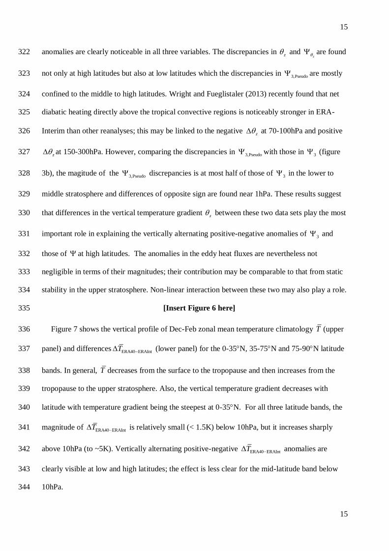
[Insert Figure 6 here] 335
Figure 7 shows the vertical profile of Dec-Feb zonal mean temperature climatology T (upper 336
panel) and differences ERA40 ERAIntT (lower panel) for the 0-35N, 35-75N and 75-90N latitude 337
bands. In general, T decreases from the surface to the tropopause and then increases from the 338
tropopause to the upper stratosphere. Also, the vertical temperature gradient decreases with 339
latitude with temperature gradient being the steepest at 0-35N. For all three latitude bands, the 340
magnitude of ERA40 ERAIntT is relatively small (< 1.5K) below 10hPa, but it increases sharply 341
above 10hPa (to ~5K). Vertically alternating positive-negative ERA40 ERAIntT anomalies are 342
clearly visible at low and high latitudes; the effect is less clear for the mid-latitude band below 343
10hPa. 344
16
16
[insert Figure 7 here] 345
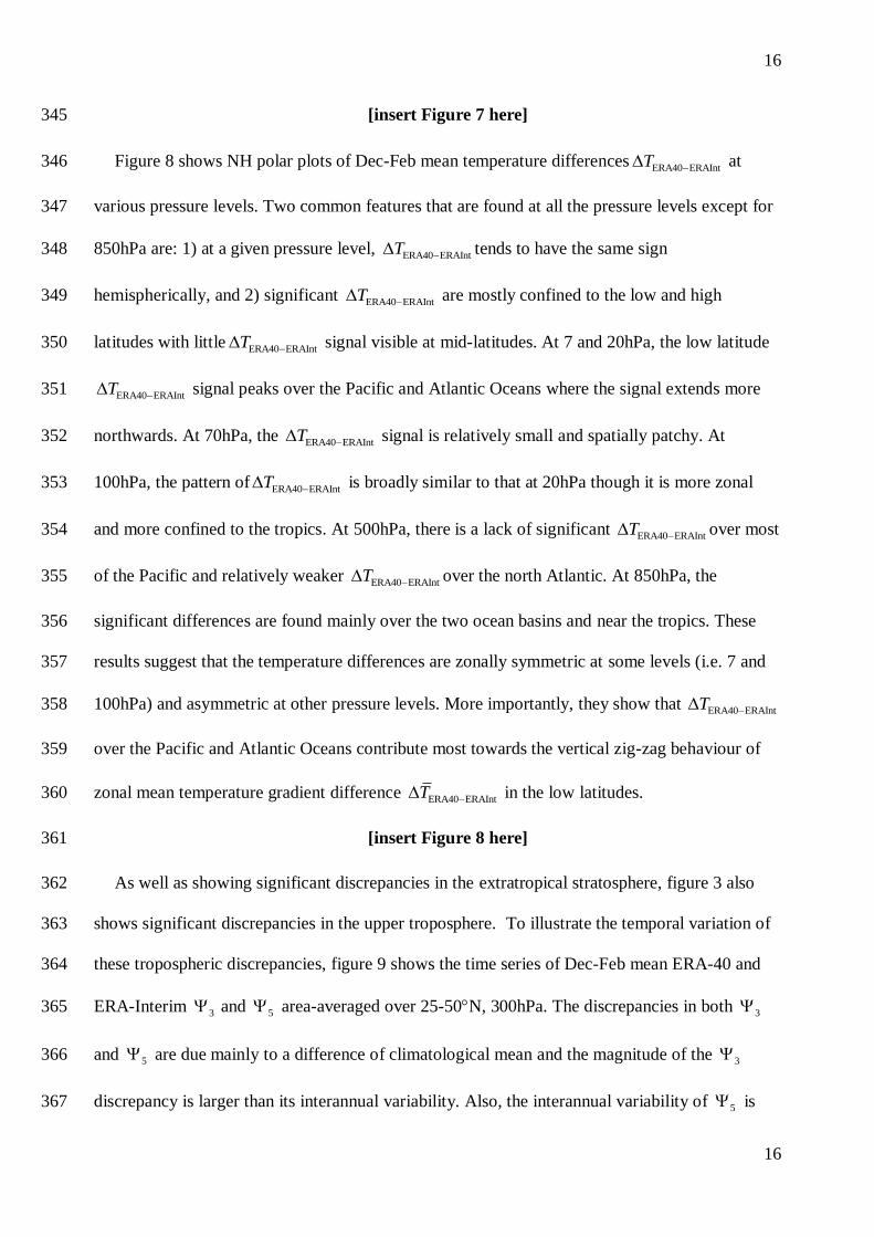
Figure 8 shows NH polar plots of Dec-Feb mean temperature differencesERA40 ERAIntT at 346
various pressure levels. Two common features that are found at all the pressure levels except for 347
850hPa are: 1) at a given pressure level, ERA40 ERAIntT tends to have the same sign 348
hemispherically, and 2) significant ERA40 ERAIntT are mostly confined to the low and high 349
latitudes with little ERA40 ERAIntT signal visible at mid-latitudes. At 7 and 20hPa, the low latitude 350
ERA40 ERAIntT signal peaks over the Pacific and Atlantic Oceans where the signal extends more 351
northwards. At 70hPa, the ERA40 ERAIntT signal is relatively small and spatially patchy. At 352
100hPa, the pattern of ERA40 ERAIntT is broadly similar to that at 20hPa though it is more zonal 353
and more confined to the tropics. At 500hPa, there is a lack of significant ERA40 ERAIntT over most 354
of the Pacific and relatively weaker ERA40 ERAIntT over the north Atlantic. At 850hPa, the 355
significant differences are found mainly over the two ocean basins and near the tropics. These 356
results suggest that the temperature differences are zonally symmetric at some levels (i.e. 7 and 357
100hPa) and asymmetric at other pressure levels. More importantly, they show that ERA40 ERAIntT 358
over the Pacific and Atlantic Oceans contribute most towards the vertical zig-zag behaviour of 359
zonal mean temperature gradient difference ERA40 ERAIntT in the low latitudes. 360
[insert Figure 8 here] 361
As well as showing significant discrepancies in the extratropical stratosphere, figure 3 also 362
shows significant discrepancies in the upper troposphere. To illustrate the temporal variation of 363
these tropospheric discrepancies, figure 9 shows the time series of Dec-Feb mean ERA-40 and 364
ERA-Interim 3 and 5 area-averaged over 25-50N, 300hPa. The discrepancies in both 3 365
and 5 are due mainly to a difference of climatological mean and the magnitude of the 3 366
discrepancy is larger than its interannual variability. Also, the interannual variability of 5 is 367
17
17
much larger than that of 3 ; 5 may play a dominant role in the total waving forcing for a 368
particular winter such as 1989 in this region. 369
[insert Figure 9 here] 370
Figure 3 shows that 5 is also responsible for the total wave forcing discrepancies in the low 371
latitude upper troposphere. To illustrate the temporal variation of these discrepancies, figure 10 372
shows the time series of ERA-40 and ERA-Interim 5 that are area-averaged over 0-10N, 373
300hPa (left) and 0-10N, 100hPa (right). The discrepancies are again dominated by a difference 374
in climatological mean. The climatological difference in 5 at 300hPa is again larger than its 375
interannual variability, implying that there is large uncertainty associated with the momentum 376
budget in this region. Apart from the dominant climatological mean difference, there are also 377
noticeable disagreements in the interannual variability in 5 at 300hPa. It is noted that ERA-378
Interim 5 departs further away from the zero line than ERA-40 5 at both 100hPa and 379
300hPa, implying a larger magnitude of the vertical eddy flux ' 'w u in ERA-Interim than ERA-380
40. Small-scale processes such as gravity waves play an important role in ' 'w u (Lindzen 1981), 381
differences in model resolution and parameterization are the likely sources for the discrepancies. 382
It has been shown that the vertical velocity of ERA-Interim is less noisy than that of ERA-40 383
(Dee and Uppala 2008; Iwasaki et al. 2009). This may also contribute to the larger magnitude of 384
' 'w u (or 5 ) in ERA-Interim than ERA-40. 385
[insert Figure 10 here] 386
3.2 Effect on the B-D Circulation 387
This section investigates the extent to which the resolved wave forcing term is linked to the 388
discrepancies in the B-D circulation by examining the momentum budget of TEM equation. The 389
first row of figure 11 shows the climatology of the Dec-Feb mean residual mean meridional 390
18
18
circulation ( *, *)v w (arrows) and the residual mean meridional circulation term (contours) 391
estimated from ERA-40 and ERA-Interim (figure 11a;b), as well as their composite differences 392
between these two data sets (figure 11c). The main climatological feature of the residual mean 393
meridional circulation in both ERA-40 and ERA-Interim is the upward movement of streamlines 394
of the flow at low latitudes that is followed by poleward movement at middle-latitudes and 395
finally downward movement at high latitudes. The residual meridional circulation term is 396
mainly positive, reflecting eastward (or westerly) acceleration and a predominantly northward 397
apparent force on the fluid parcels. In the stratosphere, peaks in the extra-tropical upper 398
stratosphere and it is in approximate balance with the peak in the same region (see figure 399
1a;b). The tropospheric peaks poleward of 40N where is also in rough balance with . 400
However, is not in balance with near the tropospheric subtropical jet, where gravity wave 401
drag and up-gradient eddy transport (McFarlane 1987; Birner et al. 2013) play an important role. 402
In the TEM formulation (eq. (1)), the effect of these processes is accounted for by the non-403
conservative term X rather than the resolved wave forcing term , suggesting that the effects of 404
parameterized processes such as the gravity wave drag and numerical approximation play a 405
important role in this region. 406
[insert Figure 11 here] 407
The key feature of the discrepancies in the residual circulation is the broadly positive 408
ERA40-ERAInt between 2-200hPa together with the poleward arrows in the same region (figure 409
11c). This implies a stronger residual circulation in ERA-40 than ERA-Interim, which is 410
consistent with other studies (e.g. Iwasaki et al. 2009; Fueglistaler et al. 2013; Monge-Sanz et al. 411
2013). However, the regions with significant positive ERA40-ERAInt do not generally coincide with 412
the regions of significant negative ERA40-ERAInt or vice versa (see figure 1c). The only 413
exceptions are the mid-latitude upper stratosphere (20-40N, 2-7hPa) and the high latitude upper 414

19
19
troposphere and lower stratosphere (poleward of 70N, 500-30hPa), where ERA40-ERAInt partially 415
cancelsERA40-ERAInt . Therefore, the discrepancies in the E-P flux divergence can only partially 416
explain the discrepancies in the residual circulation. 417
The second row of figure 11 shows the climatology of the non-conservative term X 418
(contours) calculated asdu
dt from ERA-40 and ERA-Interim (figure 11d;e), as well as 419
the composite differences of X between these two data sets (figure 11f). Above 100hPa, the 420
climatology of X is mainly negative for both data sets. This implies that other processes, such 421
as small-scale wave forcing, are also involved in driving the residual meridional circulation 422
(Seviour et al. 2012). Note that Seviour et al. (2012) found smaller magnitudes of the non-423
conservative term X than those shown in figure 11e for ERA-Interim. This is likely because our 424
results are based on daily averaged data at 2.5 by 2.5 resolution and for the period of 1979-425
2002 while Seviour et al. (2012) used 6-hourly instantaneous records at 3.75 by 2.5 resolution 426
for the period 1989-2009. 427
The magnitude of stratospheric X differs between these two data sets; it is nearly twice as 428
large in ERA-40 than in ERA-Interim. This results in hemisphere-wide significant negative 429
ERA40 ERAIntX above 200hPa, except for the high latitude upper stratosphere where gravity waves 430
may play an important role (Holton 1983). The stratospheric ERA40 ERAIntX is broadly in balance 431
with ERA40 ERAInt (see figure 11c), implying that the balance between terms other than X is 432
better achieved in ERA-Interim than ERA-40. Because the zonal wind tendency u t term for 433
the Dec-Feb mean is at least one magnitude smaller than either or in terms of both the 434
climatology and the differences (not shown) and the differences in the zonal mean zonal wind u 435
between these two data sets are negligibly small (Dee et al. 2011a; Lu et al. 2014), results shown 436
20
20
in figures 1c and 11c;f indicate that the discrepancies in none of , or X have corresponding 437
differences in zonal mean flow. 438
In the upper troposphere, X is largely in balance with in terms of climatology (see figure 439
1a;b). Especially, both data sets show a good balance between X and at 15-55N, 150-440
300hPa. As such, the TEM budget based on the resolved wave forcing becomes inadequate for 441
the assessment of the forced variability of zonal wind in this region. Figure 11f suggests that this 442
nonlinear interaction appears to occur lower in altitude in ERA-40 than ERA-Interim, resulting 443
in the positive ERA40 ERAIntX centred at 20-50N, 300hPa; the difference may be attributed to the 444
stronger convective motion and therefore more effective vertical heat transport in ERA-Interim 445
(Wright and Fueglistaler 2013). 446
In the tropical upper troposphere, ERA40 ERAIntX is mostly in balance with ERA40 ERAInt , 447
implying that ERA-40 and ERA-Interim account for large-scale wave forcing and the non-448
conservative processes differently in this region. Similar to those at 15-55N, 150-300hPa, the 449
discrepancies are closely associated with analysis increments of temperature in the region, where 450
the interaction between temperature, vertical velocity and humidity is better captured by ERA-451
Interim than ERA-40 (Dee and Uppala 2009; Dee et al. 2011a). Differences in gravity wave 452
parameterization may also contribute to these tropical discrepancies (McFarlane 1987). 453
3.3 Sudden change of Mean in the Eddy Heat Fluxes 454
Up to this point, the diagnostics have been based on the composite differences between the 455
two data sets for their common period; they therefore do not address the discrepancies in long-456
term trends. Inhomogeneity in either temperature gradient z or wave fluxes can induce trend 457
uncertainty of the wave forcing. Because the poleward eddy heat flux ' 'v T is the most important 458
quantity for assessing the impact of tropospheric waves propagating into the stratosphere, it is 459
chosen here to identify possible discontinuities that are induced by a change of instruments, or 460
21
21
quantity and quality of observations over time. Similar analysis can also be performed for 461
temperature gradient z , but only the results of ' 'v T are reported here as a demonstration. 462
In this section, we use the PMT technique to detect any significant sudden departure of ' 'v T 463
difference between the two reanalyses, i.e. ERA40 -ERAInt
' 'v T . The reason that we use 464
ERA40 -ERAInt
' 'v T rather ERA40' 'v T or ERAInt' 'v T for the detection is because the PMT technique 465
requires that the time series under consideration is normally distributed and does not have a 466
physically real trend. It is more likely that ERA40 -ERAInt
' 'v T satisfies the “no-trend” assumption 467
because any apparent trend in ERA40 -ERAInt
' 'v T is more likely to be caused by a discontinuity of 468
observations or an inhomogeneity in the treatment of observations by the data assimilation 469
procedure in one or both of the data sets. Conversely, ERA40' 'v T and ERAInt' 'v T are more likely to 470
combine physically real trends with instrumental-induced sudden changes, violating the “no-471
trend” requirement of the PMT. For the same reason, ERA40 -ERAInt
' 'v T is more likely to obey a 472
normal distribution due to the random nature of the observational errors, except for the sudden 473
changes. Most importantly, for each individual time series ERA40' 'v T or ERAInt' 'v T , the 474
magnitudes of the discontinuity and the trend are much smaller than that of the interannual 475
variability, making it statistically harder to detect the changepoint. But because the two time 476
series are very strongly co-varying (see figure 5 for instance), taking the difference allows us to 477
effectively remove the interannual variability and thus to detect the small discontinuity. 478
Figure 12 shows the time series of Dec-Feb mean total, stationary and transient eddy heat flux 479
' 'v T averaged over 10-30N, 100hPa, from ERA-40 (blue dashed), ERA-Interim (red dash-480
dotted) and their difference (black solid). It appears that both total and stationary 10-30N,100hPa' 'v T 481
in ERA-40 have long-term downward trends, which becomes noticeably steeper after the 1991 482
22
22
winter; those in ERA-Interim 10-30N,100hPa' 'v T however have no obvious trends. An immediate 483
sudden departure between ERA-40 and ERA-Interim in both total and stationary 10-30N,100hPa' 'v T484
can be clearly seen after the 1991winter with ERA-Interim estimates being consistently larger 485
than those of ERA-40 after this time. A different behavior can be observed for the transient 486
component, with ERA-40 estimates being consistently larger than those of ERA-Interim before 487
the 1997 winter and the two estimates becoming more nearly identical to each other after 1997. 488
According to the three significance measures, a significant changepoint in the wave forcing 489
difference ERA40 -ERAInt
' 'v T is detected in the 1991 winter, after which the total 490
ERA40 -ERAInt
' 'v T and its stationary values dropped significantly. The drop is most noticeable in 491
the stationary component, which has a zero mean for the period 1980-1991 but a mean value of 492
1.5 K m s1
in the period 1992-2002. The drop is about half of the amplitude of its interannual 493
variability. There is another possible changepoint in the winter of 1997, after which the transient 494
component of ERA40 -ERAInt
' 'v T appeared to drop suddenly. For the 1997 changepoint, 495
however, only two of the three p-values are significant at the 0.05 level. 496
[insert Figure 12 here] 497
Figure 13a shows a NH polar plot of Dec-Feb mean eddy heat flux ' 'v T at 100hPa estimated 498
using ERA-Interim while figure 13b shows the composite difference of ERA40 -ERAInt
' 'v T at 499
100hPa between the periods 1992-2002 and 1980-1991 (i.e. later minus earlier periods). The 500
climatological ' 'v T peaks at 45-75N and attains its maximum value (~80 K m s-1
) over the 501
North Pacific Ocean. The overall pattern of ' 'v T resembles those of previous studies and it is 502
known to be controlled by the stationary component that is related to near surface topography 503
and topographically induced perturbations (e.g. Plumb 1985; Newman and Nash 2000). 504
[insert Figure 13 here] 505
23
23
Figure 13b shows the difference plot of total ERA40 -ERAInt
' 'v T after and before 1991 (later 506
minus earlier periods). The sudden change of ERA40 -ERAInt
' 'v T in 1991 is mainly marked by a 507
longitudinal belt of negative anomalies centred on 20N. The largest jump is located near the 508
vicinity of Mt. Pinatubo and there are significant negative anomalies almost everywhere in 509
radiosonde-data sparse ocean regions in the latitude band of 10-30N. The stationary component 510
accounts for almost all of these negative anomalies (not shown). In the mid- to high latitudes, the 511
values of ERA40 -ERAInt
' 'v T are predominately positive. The magnitude of those positive 512
anomalies is found to be noticeably enhanced in the stationary component while significant 513
negative anomalies of transient ERA40 -ERAInt
' 'v T are found at 70-80N (not shown). These 514
high latitude positive/negative differences in the stationary/transient component imply that the 515
1991 sudden jump induced an upward/down trend in the respective component of ERA-40 516
45 75N, 100hPa' 'v T (see figure 5). 517
Figure 14 shows the time series of Dec-Feb mean total, stationary and transient ' 'v T 518
averaged over 45-75N at 10hPa, estimated from ERA-40, ERA-Interim and their difference. 519
The total, stationary and transient 45-75N,10hPa' 'v T show similar behaviors as 45-75N,10hPa' 'v T (see the 520
right hand panels of figure 4), with the two data sets closely resembling each other. However, 521
based on the three significance measures, a significant changepoint is detected in 1998 winter for 522
the difference between these two data sets ERA40 -ERAInt
' 'v T . After the 1998 winter, the total 523
and stationary ERA40 -ERAInt
' 'v T dropped significantly. The transient ERA40 -ERAInt
' 'v T also 524
dropped after 1998 though the third measure does not attain a p-value 0.05. However, the 525
detection of a change after 1998 at 10hPa involves a comparison between a 4-year interval that 526
exhibits large ' 'v T anomalies (i.e. 1999-2002) with a 19-year period of relatively small ' 'v T527
anomalies (i.e. 1980-1998). The relative size of the drop, at ~5-7% of the climatological mean 528
24
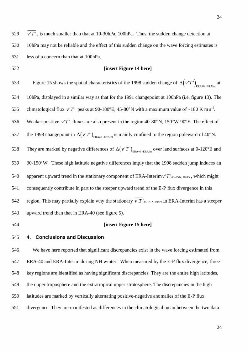
24
' 'v T , is much smaller than that at 10-30hPa, 100hPa. Thus, the sudden change detection at 529
10hPa may not be reliable and the effect of this sudden change on the wave forcing estimates is 530
less of a concern than that at 100hPa. 531
[insert Figure 14 here] 532
Figure 15 shows the spatial characteristics of the 1998 sudden change of ERA40 -ERAInt
' 'v T at 533
10hPa, displayed in a similar way as that for the 1991 changepoint at 100hPa (i.e. figure 13). The 534
climatological flux ' 'v T peaks at 90-180E, 45-80N with a maximum value of ~180 K m s-1
. 535
Weaker positive ' 'v T fluxes are also present in the region 40-80N, 150W-90E. The effect of 536
the 1998 changepoint in ERA40 -ERAInt
' 'v T is mainly confined to the region poleward of 40N. 537
They are marked by negative differences of ERA40 -ERAInt
' 'v T over land surfaces at 0-120E and 538
30-150W. These high latitude negative differences imply that the 1998 sudden jump induces an 539
apparent upward trend in the stationary component of ERA-Interim 45 75N, 10hPa' 'v T , which might 540
consequently contribute in part to the steeper upward trend of the E-P flux divergence in this 541
region. This may partially explain why the stationary 45 75N, 10hPa' 'v T in ERA-Interim has a steeper 542
upward trend than that in ERA-40 (see figure 5). 543
[insert Figure 15 here] 544
4. Conclusions and Discussion 545
We have here reported that significant discrepancies exist in the wave forcing estimated from 546
ERA-40 and ERA-Interim during NH winter. When measured by the E-P flux divergence, three 547
key regions are identified as having significant discrepancies. They are the entire high latitudes, 548
the upper troposphere and the extratropical upper stratosphere. The discrepancies in the high 549
latitudes are marked by vertically alternating positive-negative anomalies of the E-P flux 550
divergence. They are manifested as differences in the climatological mean between the two data 551

25
25
sets and can account for up to 15-45% of the interannual variability in the affected region. Such 552
discrepancies are due mainly to differences in the vertical gradient of potential temperature z . 553
Similar vertically alternating positive-negative anomalies were previously found in the 554
analysis increments of temperature in many reanalysis data sets and are known to be caused by 555
the presence of systematic bias between the data assimilation model and the satellite 556
measurements (Uppala et al. 2005; Dee and Uppala 2009; Kobayashi et al. 2009). Such a bias 557
has a larger magnitude and is more persistent in ERA-40 than ERA-Interim (Simmons et al. 558
2007; Dee and Uppala 2009). Recent studies indicate much closer agreement to observations by 559
ERA-Interim compared to ERA-40 and it is attributed to the advances in the ERA-Interim 560
assimilation system, especially the various improvements of the ERA-Interim 4D-Var system 561
over the previous 3D-Var system that was used by ERA-40 (e.g. Fueglistaler et al. 2009; Dee et 562
al. 2011a; Simmons et al. 2010, 2014; Bracegirdle and Marshall 2012). For this reason, we 563
suggest the E-P flux divergence discrepancies at high latitudes are most likely due to the model 564
drift induced by the data assimilation system, instead of observational errors. 565
In the middle to low latitude upper troposphere, the discrepancies in the E-P flux divergence 566
are due largely to the bias in the vertical momentum flux ' 'w u . It has been suggested that 567
imbalance of radiative heating induced by assimilation of the observational radiance data tends 568
to introduce noise in the vertical velocity (Schoeberl et al. 2003; Fueglistaler et al. 2009). More 569
importantly, because small-scale processes such as convection and gravity waves may contribute 570
significantly to the momentum budget in addition to resolved wave forcing, differences in model 571
resolution and parameterization of sub-grid processes by ERA-40 and ERA-Interim can induce 572
discrepancies in the E-P flux divergence in this region. This may explain why the discrepancies 573
are marked by a cancellation between the E-P flux divergence term and the non-conservative 574
term X . These discrepancies may also be linked to the large bias of analysis increments in the 575
tropical upper troposphere (Dee and Uppala 2009). Furthermore, we have noted that the 576
26
26
discrepancy in the E-P flux divergence climatology can be larger than the amplitude of its 577
interannual variation in this region; such large uncertainty strongly discourages merging these 578
two reanalysis products to study wave mean flow interaction. 579
In the upper stratosphere, the E-P flux divergence discrepancies involve all the relevant flux 580
terms and are associated with substantial differences in temperature as well as static stability. 581
These discrepancies may be attributed to the relatively larger model bias in the region, where 582
observations are sparse and model errors are large (Dee and Uppala 2009). Nevertheless, we 583
find that the discrepancies between these two data sets become much reduced both in terms of 584
interannual variability, climatological mean and long-term trend if the wave forcing is measured 585
by the poleward eddy heat flux ' 'v T . 586
Based on the TEM momentum budget, we have shown that a stronger residual circulation is 587
associated with ERA-40 than ERA-Interim, agreeing with previous studies (e.g. van Noije et al. 588
2004; Monge-Sanz et al. 2007; Dee and Uppala 2009; Monge-Sanz et al. 2013). However, the 589
discrepancies in the residual circulation are only partially associated with the discrepancies in the 590
resolved, large-scale wave forcing. The majority of the discrepancies in the residual circulation 591
are associated with the non-conservative term X , suggesting that the bias in wave forcing is not 592
the main cause for the excessively strong B-D circulation in ERA-40. The excessively strong B-593
D circulation in ERA-40 was in part attributed to systematic analysis increments in stratospheric 594
temperature that resulted from the biases induced by the 3D-Var assimilation (Uppala et al. 595
2005). Apart from radiative heating, improvements in the treatment of the effects of volcanic 596
aerosols, gravity wave drag, and better radiation schemes may also have led to an improved 597
representation of the B-D circulation in ERA-Interim (Dee et al. 2011a). Especially, it is known 598
that gravity wave drag plays a considerable role in driving the B-D circulation (McLandress and 599
Shepherd 2009; Butchart et al. 2010; Seviour et al. 2012) and the effect of smaller scale wave 600
drag is better resolved by ERA-Interim than ERA-40 (Dee and Uppala 2009; Dee et al. 2011a). 601
27
27
A recent study shows that the largest differences in radiative heating in the tropical upper 602
troposphere between several reanalysis products are due primarily to differences in cloud 603
radiative heating as well as localized biases in heating and cooling associated with parameterised 604
turbulent mixing (Wright and Fueglistaler 2013). 605
The thermodynamical balance in the stratosphere is largely a balance between the radiative 606
heating and the dynamical heating from the advection of the residual circulation (Andrews et al. 607
1987). Because the dynamical heating term in the thermodynamical budget of the TEM 608
equations is the product of the residual velocity and the temperature gradients, an enhanced 609
residual circulation should be associated with cooling in the low latitude stratosphere and 610
warming at high latitudes if the radiative heating is constant. However, the temperature 611
difference ERA40 ERAIntT in the tropical lower stratosphere (70-100hPa) is characterized by 612
significant warm anomalies at 0-35N (see figure 8) and an enhanced B-D circulation (see figure 613
11). This is opposite to what we would expect from the augment of dynamical heating. Thus, the 614
discrepancies in the dynamical behaviour between these two data sets are more likely the result 615
of a dynamical adaption to a difference in radiative balance. Because the wave forcing 616
discrepancies are mostly confined to the regions where analysis increments of temperatures are 617
known to be largest, we suggest that they are likely to have originated from an imbalance in 618
radiative heating that is introduced during the ingestion of observational data. However, an 619
enhanced B-D circulation and a warmer tropical lower stratosphere previously reported for the 620
ERA-40 cannot be explained only by differences in the static stability or radiative heating in the 621
high latitude stratosphere and/or in the low latitude upper troposphere. The differences may also 622
have originated from the bias in the forecast model. For instance, the forecast models may have 623
different radiative transfer scheme and/or they generate different distributions of clouds, ozone 624
and water vapor, which then leads to different radiative heating. Further studies are required to 625
28
28
investigate the implications for tracer transport and ozone tendencies extracted from the 626
reanalysis data sets. 627
A sudden drop of the eddy heat flux difference ERA40 -ERAInt
' 'v T is detected after the 1991 628
winter over the subtropical ocean at ~10-30N, 100hPa. This drop could be due in part to the 629
contamination effects of volcanic aerosols on the infrared radiances measured by the High 630
Resolution Infrared Radiation Sounder (HIRS) on board the NOAA-12 satellite following the 631
eruption of Mt. Pinatubo in June, 1991 (Uppala et al. 2005). Because the radiative transfer 632
model that was used by ERA-40 did not include the effect of volcanic aerosols, the aerosol 633
contaminated radiance measurements were absorbed by the bias corrections of the 3D-Var 634
assimilation system, which is known to result in excessive humidity/rainfall in the tropics and 635
subtropics (Uppala et al. 2005; Dee and Uppala 2009). A revised thinning, channel-selection and 636
quality control of HIRS radiances assimilation was used by ERA-Interim, in which the 4D-Var 637
analysis system couples the humidity and the dynamic variables cohesively to help ensure a 638
realistic interaction between temperature, vertical velocity and humidity (Dee and Uppala 2009; 639
Dee et al. 2011a). 640
A subtler sudden drop in eddy heat flux difference ERA40 -ERAInt
' 'v T is also detected in the 641
mid-latitudes at 10hPa. This drop may be linked to the discontinuity in upper-stratospheric 642
temperatures associated with the radiance measurements from the Advanced Microwave 643
Sounding Unit-A (AMSU-A) since August 1998 in ERA-Interim (Dee and Uppala 2008). While 644
the ERA-40 reanalysed temperatures in the upper stratosphere inherited a consistent warm bias 645
from the assimilation model, ERA-Interim however began using uncorrected radiance data from 646
AMSU-A channel 14 from August 1998 (Dee and Uppala 2008). This change is known to have 647
induced a jump of the global mean temperature above 10 hPa in ERA-Interim (Dee and Uppala 648
2008). It remains unknown whether or not this change caused a jump of ' 'v T in ERA-Interim or 649

29
29
if instead the detected sudden drop of ERA40 -ERAInt
' 'v T after the 1998 winter is due mainly to a 650
change of correlation coefficient between temperature T and meridional velocity v. 651
Several studies have found significant trends in stratospheric wave forcing (Newman and 652
Nash 2000; Randel et al. 2002; Hu and Tung 2002) while others have found that the trends 653
reverse in early and later winter with no significant trend in mid-winter (Karpetchko and Nikulin 654
2004; Hu et al. 2005). Here, we have found that trends in the E-P flux divergences differ 655
substantially between these two data sets. Sudden changes in either temperature gradient or eddy 656
fluxes that are induced by inhomogeneity of observations are able to alter the respective trends 657
and low frequency variability in the wave forcing. Because the highly derived nature of the E-P 658
flux divergence, the trends estimated from such a quantity should be treated with extreme 659
caution. 660
Nevertheless, we have found that the trends in the eddy heat flux ' 'v T are more consistent 661
than those in the E-P flux divergence. In both ERA-40 and ERA-Interim in the mid-latitude 662
stratosphere there is a positive trend in the stationary ' 'v T and a negative trend in the transient663
' 'v T , generally in agreement with previous studies (Newman and Nash 2000; Randel et al. 664
2002). It must be noted that the general circulation model (GCM) used in both ERA-40 and 665
ERA-Interim does not include the effect of solar variability; any decadal to multi-decadal scale 666
variation comes solely from the observations (Dee et al. 2011a). During solar maxima, the 667
background state that is predicted by the GCM of the data assimilation system is generally biased 668
compared to the observations, so systematic analysis increments may emerge as a result. This 669
can affect the low-frequency variation and the trends for both data sets. Thus, further 670
confirmation based on longer records and other reanalysis data sets is needed before we can go 671
further into the physical explanations of the opposite trends in the stratosphere in terms of the 672
stationary and transient ' 'v T . 673

30
30
This comparative study of wave forcing estimated from ERA-40 and ERA-Interim provides 674
an additional perspective for evaluating dynamic processes in the stratosphere and upper 675
troposphere. It is noted that a comparative study like this cannot make a quantitative attribution 676
in terms of which data set is better and/or by how much. Our results nevertheless show that bias 677
in static stability induced by temperature differences and/or radiative heating imbalance can 678
potentially cause large uncertainty in the E-P flux divergence, endorsing the importance of 679
reducing the analysis increments especially the model drift in assimilating temperatures. Our 680
results also demonstrate the importance of the recently established Stratospheric Processes and 681
their Role in Climate (SPARC) Renalysis/analysis Intercomparison Project (S-RIP) (Fujiwara et 682
al., 2012; Fujiwara and Jackson, 2013). 683
684
Acknowledgements: This study is part of the British Antarctic Survey Polar Science for Planet 685
Earth Programme funded by the Natural Environment Research Council. We acknowledge use of 686
ECMWF reanalysis data sets and documentation at http://www.ecmwf.int. We would also like to 687
thank the three reviewers for their detailed and constructive comments. 688
689

31
31
Appendix: Penalized maximal t-test 690
Let , 1,2,...,tX t N denote a time series with zero true trend (but potentially containing a 691
sudden change that may give rise to an apparent linear trend in tX ) and identically and 692
independently distributed (IID) Gaussian errors. To detect a changepoint in tX is to test the 693
null hypothesis 694
2
0 : ~ IID ,tH X N 695
against the alternative 696
2
1
2
2
~ IID , , 1,...,:
~ IID , , 1,...,
t
c
t
X t kH
X t k N
N
N 697
where 1 2 and 2~ IID ,tX N stands for tX follows an IID Gaussian distribution 698
of mean and variance 2 . When cH is true, the entire time series tX can be viewed as two 699
independent samples from two normal distributions of the same unknown variance 2 , one for 700
all t k and another for all t > k, where the point/time t = k is called a changepoint, and 701
1 2 is called the magnitude of the mean shift. 702
To detect the most probable value of k and to test whether the means of these two samples 703
are statistically significantly different from each other, the test statistic for detecting a mean shift 704
by penalized maximal t-test is 705
max 1 1PT max ( ) ( ) ,k N P k T k 706
where 707
1/2
1 2
1 ( )( ) ,
k
k N kT k X X
N
708
1 2
1 1
1 1, ,
k N
t t
t t k
X X X Xk N k
709
32
32
2 22
1 2
1 1
1ˆ
2
k N
k t t
t t k
X X X XN
710
and ( )P k is an empirical penalty function that is constructed via Monte Carlo simulation 711
according to N and k (Wang et al. 2007). The functional form of ( )P k is constructed to give the 712
same level of confidence on the detected changepoints regardless of their position in the time 713
series tX and to have the same false-alarm rate for all points if tX happens to be a 714
homogeneous series. The empirical weight function ( )P k is used to diminish the effect of 715
unequal sample sizes on the power of detection only based on ( )T k so that the false-alarm rate of 716
PMT is evenly distributed across all candidate changepoints. The detailed formulation of ( )P k is 717
given in Wang et al. (2007). 718
Here, we use three measures to evaluate the significance of any detected changepoint. The 719
first measure is the chance of a changepoint occurring at the detected position; the second 720
measure is the significance of the mean-shift magnitude , and the third measure is the 721
significance of the maximum value of the penalized t-statistics maxPT . To calculate these three 722
measures, 10,000 synthetic random time series that share the same distribution of 723
2IID , N are constructed based on Monte Carlo simulations. To calculate the first 724
measure, the PMT detection is performed to find the position k in the time series where the 725
maximum value of ( ) ( )P k T k exists for each synthetic series. A distribution of the random trial 726
based k values is then constructed accordingly. The k value estimated from the original time 727
series is compared to this distribution and the rank of the actual k among these randomized trials 728
determines its significance level. To calculate the second measure, we rank the true values 729
against the distribution of calculated from the 10,000 synthetic series. Similarly, the third 730
measure is established by ranking the maximum value of ( ) ( )P k T k of the actual series against 731
those from the synthetic series. When the ranks for all the three measures fall in the 5% tail-ends 732

33
33
of their associated distributions, the changepoint is regarded as statistically significant. For 733
simplicity, we call the proportional ranks as p-values in order to align with the traditional 734
terminology of significance tests.735
34
34
References: 736
Andrews, D. G., J. R. Holton, and C. B. Leovy, 1987: Middle Atmosphere Dynamics Academic Press INC. LTD., 737
London. 738
Bengtsson, L., and Coauthors, 2007: The need for a dynamical climate reanalysis. Bull. Amer. Meteor. Soc., 88, 495-739
501. 740
Berrisford, P., and Coauthors, 2011: Atmospheric conservation properties in ERA-Interim. Quart. J. Roy. Meteor. 741
Soc., 137, 1381-1399. 742
Birner, T., and H. Bonisch, 2011: Residual circulation trajectories and transit times into the extratropical lowermost 743
stratosphere. Atmos. Chem. Phys., 11, 817-827. 744
——, D. W. J. Thompson, and T. G. Shepherd 2013: Up-gradient eddy fluxes of potential vorticity near the 745
subtropical jet, Geophys. Res. Lett., 40, doi:10.1002/2013GL057728. 746
Bracegirdle, T. J., G. J. Marshall, 2012: The reliability of Antarctic tropospheric pressure and temperature in the 747
latest global reanalyses. J. Climate, 25, 7138-7146. 10.1175/JCLI-D-11-00685.1. 748
Butchart, N., and Coauthors, 2010: Chemistry-climate model simulations of twenty-first century stratospheric 749
climate and circulation changes. J. Climate, 23, 5349-5374. 750
Cornes, R., and P. Jones, 2013: How well does the ERA-Interim reanalysis replicate trends in extremes of surface 751
temperature across Europe? J. Geophys. Res., 118, 10262-10276. 752
Dee, D. P., 2005: Bias and data assimilation, Quart. J. Roy. Meteor. Soc., 131, 3323– 3343, doi:10.1256/qj.05.137. 753
——, and S, Uppala, 2008: Variational bias correction in ERA-Interim, ECMWF Technical Memorandum, No. 575. 754
——, and S. Uppala, 2009: Variational bias correction of satellite radiance data in the ERA-Interim reanalysis. 755
Quart. J. Roy. Meteor. Soc., 135, 1830-1841. 756
——, and Coauthors, 2011a: The ERA-Interim reanalysis: configuration and performance of the data assimilation 757
system. Quart. J. Roy. Meteor. Soc., 137, 553-597. 758
——, E. Källén, A. J. Simmons, and I. Haimberger 2011b: Comments on ‘Reanalyses suitable for characterizing 759
long-term trends’, Bull. Am. Meteorol. Soc., 92, 65-70, doi: 10.1175/2010BAMS3070.1. 760
Dima, I., and J. Wallace, 2007: Structure of the annual-mean equatorial planetary waves in the ERA-40 reanalyses. 761
J. Atmos. Sci., 64, 2862-2880. 762
Edmon, H., B. Hoskins, and M. McIntyre, 1980: Eliassen-PalM cross-sections for the troposphere. J. Atmos. Sci., 763
37, 2600-2616. 764
Fujiwara, M. and D. Jackson, 2013: SPARC Reanalysis Intercomparison Project (S-RIP) Planning Meeting, SPARC 765
Newsletter, 41, 52–55. 766
Fujiwara, M., S. Polavarapu, and D. Jackson, 2012: A proposal of the SPARC Reanalysis/Analysis Intercomparison 767
Project, SPARC Newsletter, 38, 14–17, 2012. 768
Fueglistaler, S., and Coauthors, 2009: The diabatic heat budget of the upper troposhere and lower/mid stratosphere 769
in ECMWF reanalyses. Quart. J. Roy. Meteor. Soc., 135, 21-37. 770
Hólm, E., E. Andersson, A. Beljaars, P. Lopez, J.-F. Mahfouf, A. J. Simmons, and J.-N. Thépaut, 2002: 771
Assimilation and modelling of the hydrological cycle: ECMWF’s status and plans. ECMWF Tech. Memo 383, 772
55 pp. 773
Holton, J. R., 1983: The influence of gravity wave breaking on the general circulation of the middle atmosphere. J. 774
Atmos. Sci., 40, 2497-2507. 775

35
35
——, P. Haynes, M. McIntyre, A. Douglass, R. Rood, and L. Pfister, 1995: Stratosphere-troposphere exchange. Rev. 776
Geophys., 33, 403-439. 777
Hu, Y., and K. Tung, 2002: Interannual and decadal variations of planetary wave activity, stratospheric cooling, and 778
Northern Hemisphere Annular mode. J. Climate, 15, 1659-1673. 779
——, ——, and J. Liu, 2005: A closer comparison of early and late-winter atmospheric trends in the northern 780
hemisphere. J. Climate, 18, 3204-3216. 781
Ingleby, N. B. 2001: The statistical structure of forecast errors and its representation in The Met. Office Global 3-D 782
Variational Data Assimilation Scheme. Quart. J. Roy. Meteor. Soc., 127, 209–231. 783
Iwasaki, T., H. Hamada, and K. Miyazaki, 2009: Comparisons of Brewer-Dobson Circulations diagnosed from 784
Reanalyses. J. Meteor. Soc. Japan, 87, 997-1006. 785
Karpetchko, A., and G. Nikulin, 2004: Influence of early winter upward wave activity flux on midwinter circulation 786
in the stratosphere and troposphere. J. Climate, 17, 4443-4452. 787
Kerr-Munslow, A., and W. Norton, 2006: Tropical wave driving of the annual cycle in tropical tropopause 788
temperatures. Part I: ECMWF analyses. J. Atmos. Sci., 63, 1410-1419. 789
Kobayashi, S., M. Matricardi, D. Dee, and S. Uppala, 2009: Toward a consistent reanalysis of the upper stratosphere 790
based on radiance measurements from SSU and AMSU-A. Quart. J. Roy. Meteor. Soc., 135, 2086-2099. 791
Lindzen, R. S. 1981: Turbulence and stress owing to gravity wave and tidal breakdown, J. Geophys. Res., 86, 9707-792
9714. 793
Lu, H., T. J. Bracegirdle, T. Phillips, A. Bushell, and L. Gray, 2014: Mechanisms for the Holton-Tan relationship 794
and its decadal variation, J. Geophys. Res., 119, doi: 10.1002 / jgrd.021352. 795
McLandress, C., and T. Shepherd, 2009: Simulated Anthropogenic Changes in the Brewer-Dobson Circulation, 796
Including Its Extension to High Latitudes. J. Climate, 22, 1516-1540. 797
McFarlane, N. A. 1987: The effect of orographically excited gravity wave drag on the general circulation of the 798
lower stratosphere and troposphere. J. Atmos. Sci., 44, 1775-1800. 799
Monge-Sanz, B., M. Chipperfield, A. Simmons, and S. Uppala, 2007: Mean age of air and transport in a CTM: 800
Comparison of different ECMWF analyses. Geophys. Res. Lett., 34. 801
——, ——, D. Dee, A. Simmons, and S. Uppala, 2013: Improvements in the stratospheric transport achieved by a 802
chemistry transport model with ECMWF (re)analyses: identifying effects and remaining challenges. Quart. J. 803
Roy. Meteor. Soc., 139, 654-673. 804
Monier, E., and B. Weare, 2011: Climatology and trends in the forcing of the stratospheric ozone transport. Atmos. 805
Chem. Phys., 11, 6311-6323. 806
Newman, P., and E. Nash, 2000: Quantifying the wave driving of the stratosphere. J. Geophys. Res., 105, 12485-807
12497. 808
——, E. Nash, and J. Rosenfield, 2001: What controls the temperature of the Arctic stratosphere during the spring? 809
J. Geophys. Res., 106, 19999-20010. 810
Palmer, T. N., 1981: Diagnostic study of a wavenumber-2 stratospheric sudden warming in a transformed Eulerian-811
mean formalism. J. Atmos. Sci., 38, 844–855. 812
Plumb, R., 1985: An alternative form of Andrews conservation low for quasi-geostrophic waves on a stead, 813
nonuniform flow. J. Atmos. Sci., 42, 298-300. 814
36
36
Randel, W., and E. Jensen, 2013: Physical processes in the tropical tropopause layer and their roles in a changing 815
climate. Nature Geosci., 6, 169-176. 816
——, R. Garcia, and F. Wu, 2002: Time-dependent upwelling in the tropical lower stratosphere estimated from the 817
zonal-mean momentum budget. J. Atmos. Sci., 59, 2141-2152. 818
——, 2008: Dynamical Balances and Tropical Stratospheric Upwelling. J. Atmos. Sci., 65, 3584-3595. 819
Schoeberl, M., A. Douglass, Z. Zhu, and S. Pawson, 2003: A comparison of the lower stratospheric age spectra 820
derived from a general circulation model and two data assimilation systems. J. Geophys. Res., 108. 821
Screen, J., and I. Simmonds, 2011: Erroneous arctic temperature trends in the ERA-40 reanalysis: A closer look. J. 822
Climate, 24, 2620-2627. 823
Seviour, W., N. Butchart, and S. Hardiman, 2012: The Brewer-Dobson circulation inferred from ERA-Interim. 824
Quart. J. Roy. Meteor. Soc., 138, 878-888. 825
Shepherd, T., 2007: Transport in the middle atmosphere. J. Meteor. Soc. Japan, 85B, 165-191. 826
Simmons, A. J., S. Uppala, D. Dee, and S. Kobayashi, 2007: ERAInterim: New ECMWF reanalysis products from 827
1989 onwards, ECMWF News Letter, 110, 25– 35. 828
——, K. M. Willett, P. D. Jones, P. W. Thorne, and D. P. Dee, 2010: Low-frequency variations in surface 829
atmospheric humidity, temperature, and precipitation: Inferences from reanalyses and monthly gridded 830
observational data sets, J. Geophys. Res., 115, D01110, doi:10.1029/2009JD012442. 831
——, P. Poli, D. P. Dee, P. Berrisford, H. Hersbach, S. Kobayashi, and C. Peubey, 2014: Estimating low-frequency 832
variability and trends in atmospheric temperature using ERA-Interim. Quart. J. Roy. Meteor. Soc., 140, 329–353. 833
doi: 10.1002/qj.2317. 834
Sterl, A., 2004: On the (in)homogeneity of reanalysis products. J. Climate, 17, 3866-3873. 835
Thorne, P., and R. Vose, 2010: Reanalyses suitable for characterizing long-term trends: Are they really achievable? 836
Bull. Amer. Meteor. Soc., 91, 353-361. 837
Uppala, S., and Coauthors, 2005: The ERA-40 re-analysis. Quart. J. Roy. Meteor. Soc., 131, 2961-3012. 838
van Noije, T., H. Eskes, M. van Weele, and P. van Velthoven, 2004: Implications of the enhanced Brewer-Dobson 839
circulation in European Centre for Medium-Range Weather Forecasts reanalysis ERA-40 for the stratosphere-840
troposphere exchange of ozone in global chemistry transport models. J. Geophys. Res., 109, 841
doi: 10.1029/2004JD004586. 842
Wang, X., Q. Wen, and Y. Wu, 2007: Penalized maximal t test for detecting undocumented mean change in climate 843
data series. J. Appl. Meteor. Climatol., 46, 916-931. 844
Waugh, D., W. Randel, S. Pawson, P. Newman, and E. Nash, 1999: Persistence of the lower stratospheric polar 845
vortices. J. Geophys. Res., 104, 27191-27201. 846
Wright, J. S. and S, Fueglistaler, 2013: Large differences in reanalyses of diabatic heating in the tropical upper 847
troposphere and lower stratosphere, Atmos. Chem. Phys., 13, 9565-9576, doi:10.5194/acp-13-9565-2013. 848
849
37
37
Figure Captions 850
Figure 1. Latitude-height cross section of the Dec-Feb mean E-P flux (arrows) and E-P flux divergence 851
term (contours). (a; b) climatology from ERA-40 and ERA-Interim; (c) composite difference (ERA-40 852
minus ERA-Interim). Solid and dashed contours are positive and negative divergence at the intervals of 853
±0.6, ±1.8, ±3, ±4.2 … m s-1
day-1
for climatology and ±0.3, ±0.9, ±1.5, ±2.1 … m s-1
day-1
for the 854
difference plots. The light and dark shaded areas represent p 0.1 and 0.05, estimated by two-sided 855
Student’s t-test. The plotted E-P flux vectors are shown as( ) ( )
0( , ) /zF F , with the scaling factor856
0.004899 used to adjust for the exaggerated vertical scale in the plot and a further division by the air 857
density 0 for a clearer visualization of the directions of wave propagation. The same scaling applies to 858
the E-P flux differences. 859
Figure 2. Time series of Dec-Feb mean E-P flux divergence term estimated from ERA-40 (blue 860
dashed) and ERA-Interim (red dash-dotted) area-averaged over 45-75N and at (a) 3hPa, (b) 10hPa, (c) 861
50hPa, and (d) 100hPa. 862
Figure 3. Composite differences (ERA-40 minus ERA-Interim) in the Dec-Feb E-P flux divergence terms 863
(a) 2, (b) 3, (c) 4, and (d) 5. The contours and shadings are the same as in figure 1c with the 864
exception that the statistical significance shading is omitted in regions of small differences and minor 865
dynamical significance (less than 0.3 m s-1
day-1
in magnitude). 866
Figure 4. Latitude-height cross section of the Dec-Feb mean of the potential heat flux ' 'v . (a) 867
climatology from ERA-Interim; (b) composite difference (ERA-40 minus ERA-Int). Solid and dashed 868
contours indicate positive and negative values and the shadings are the same as in figure 1b. 869
Figure 5. Time series of Dec-Feb mean total, stationary and transient components of the zonal mean eddy 870
heat flux ' 'v T (top to bottom) averaged over 45-75N, 100hPa (left) and 10hPa (right). The solid straight 871
lines are the associated trends in the ERA-40 (blue) and ERA-Interim (red) eddy heat flux components. 872
Figure 6. Latitude-height cross section of composite differences of the Dec-Feb mean of the vertical 873
gradient of potential temperature z (a ), 0
0z
z z
f
(b), and 3,Pseud 0o
lim
0
C' '
z z
f v
(c), 874
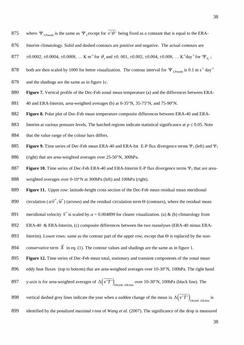
38
38
where 3,Pseudo is the same as 3 except for ' 'v being fixed as a constant that is equal to the ERA-875
Interim climatology. Solid and dashed contours are positive and negative. The actual contours are 876
0.0002, 0.0004, 0.0008, … K m-1
for z and 0. 001, 0.002, 0.004, 0.008, … K-1day
-1 for
z ; 877
both are then scaled by 1000 for better visualization. The contour interval for 3,Pseudo is 0.1 m s-1
day-1
878
and the shadings are the same as in figure 1c. 879
Figure 7. Vertical profile of the Dec-Feb zonal mean temperature (a) and the differences between ERA-880
40 and ERA-Interim, area-weighted averages (b) at 0-35N, 35-75N, and 75-90N. 881
Figure 8. Polar plot of Dec-Feb mean temperature composite differences between ERA-40 and ERA-882
Interim at various pressure levels. The hatched regions indicate statistical significance at p 0.05. Note 883
that the value range of the colour bars differs. 884
Figure 9. Time series of Dec-Feb mean ERA-40 and ERA-Int E-P flux divergence terms 3 (left) and 5 885
(right) that are area-weighted averages over 25-50N, 300hPa. 886
Figure 10. Time series of Dec-Feb ERA-40 and ERA-Interim E-P flux divergence terms 5 that are area-887
weighted averages over 0-10N at 300hPa (left) and 100hPa (right). 888
Figure 11. Upper row: latitude-height cross section of the Dec-Feb mean residual mean meridional 889
circulation (* *,v w ) (arrows) and the residual circulation term (contours), where the residual mean 890
meridional velocity *v is scaled by = 0.004899 for clearer visualization. (a) & (b) climatology from 891
ERA-40 & ERA-Interim, (c) composite differences between the two reanalyses (ERA-40 minus ERA-892
Interim). Lower rows: same as the contour part of the upper row, except that is replaced by the non-893
conservative term X in eq. (1). The contour values and shadings are the same as in figure 1. 894
Figure 12. Time series of Dec-Feb mean total, stationary and transient components of the zonal mean 895
eddy heat fluxes (top to bottom) that are area-weighted averages over 10-30N, 100hPa. The right hand 896
y-axis is for area-weighted averages of ERA40 -ERAInt
' 'v T over 10-30N, 100hPa (black line). The 897
vertical dashed grey lines indicate the year when a sudden change of the mean in ERA40 -ERAInt
' 'v T is 898
identified by the penalized maximal t-test of Wang et al. (2007). The significance of the drop is measured 899
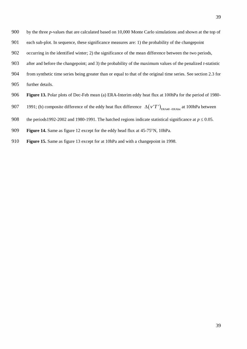
39
39
by the three p-values that are calculated based on 10,000 Monte Carlo simulations and shown at the top of 900
each sub-plot. In sequence, these significance measures are: 1) the probability of the changepoint 901
occurring in the identified winter; 2) the significance of the mean difference between the two periods, 902
after and before the changepoint; and 3) the probability of the maximum values of the penalized t-statistic 903
from synthetic time series being greater than or equal to that of the original time series. See section 2.3 for 904
further details. 905
Figure 13. Polar plots of Dec-Feb mean (a) ERA-Interim eddy heat flux at 100hPa for the period of 1980-906
1991; (b) composite difference of the eddy heat flux difference ERA40 -ERAInt
' 'v T at 100hPa between 907
the periods1992-2002 and 1980-1991. The hatched regions indicate statistical significance at p 0.05. 908
Figure 14. Same as figure 12 except for the eddy head flux at 45-75N, 10hPa. 909
Figure 15. Same as figure 13 except for at 10hPa and with a changepoint in 1998. 910
(a) (b) (c)
Figure 1. Latitude-height cross section of the Dec-Feb mean E-P flux (arrows) and E-P flux divergence term (contours). (a; b) climatology from ERA-40 and ERA-Interim; (c) composite difference (ERA-40 minus ERA-Interim) Solid and dashed contours are positive and negativedifference (ERA 40 minus ERA Interim). Solid and dashed contours are positive and negative divergence at the intervals of ±0.6, ±1.8, ±3, ±4.2 … m s-1 day-1 for climatology and ±0.3, ±0.9, ±1.5, ±2.1 … m s-1 day-1 for the difference plots. The light and dark shaded areas represent p 0.1 and 0.05,
estimated by two-sided Student’s t-test. The plotted E-P flux vectors are shown as 0)()( /),( zFF ,
with the scaling factor 004899.0 used to adjust for the exaggerated vertical scale in the plot and a further division by the air density 0 for a clearer visualization of the directions of wave propagation.
The same scaling applies to the E-P flux differences.
Figure 1Click here to download Rendered Figure: Figure1.pdf
Figure 2. Time series of Dec-Feb mean E-P flux divergence term estimated from
ERA-40 (blue dashed) and ERA-Interim (red dash-dotted) area-averaged over 45-
75N and at (a) 3hPa, (b) 10hPa, (c) 50hPa, and (d) 100hPa.
Figure 2Click here to download Rendered Figure: Figure2.pdf
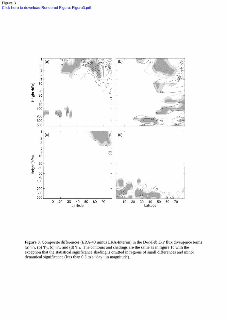
(a) (b)(a) (b)
(c) (d)
Figure 3. Composite differences (ERA-40 minus ERA-Interim) in the Dec-Feb E-P flux divergence terms (a) 2, (b) 3, (c) 4, and (d) 5. The contours and shadings are the same as in figure 1c with the exception that the statistical significance shading is omitted in regions of small differences and minor dynamical significance (less than 0 3 m s-1 day-1 in magnitude)dynamical significance (less than 0.3 m s day in magnitude).
Figure 3Click here to download Rendered Figure: Figure3.pdf
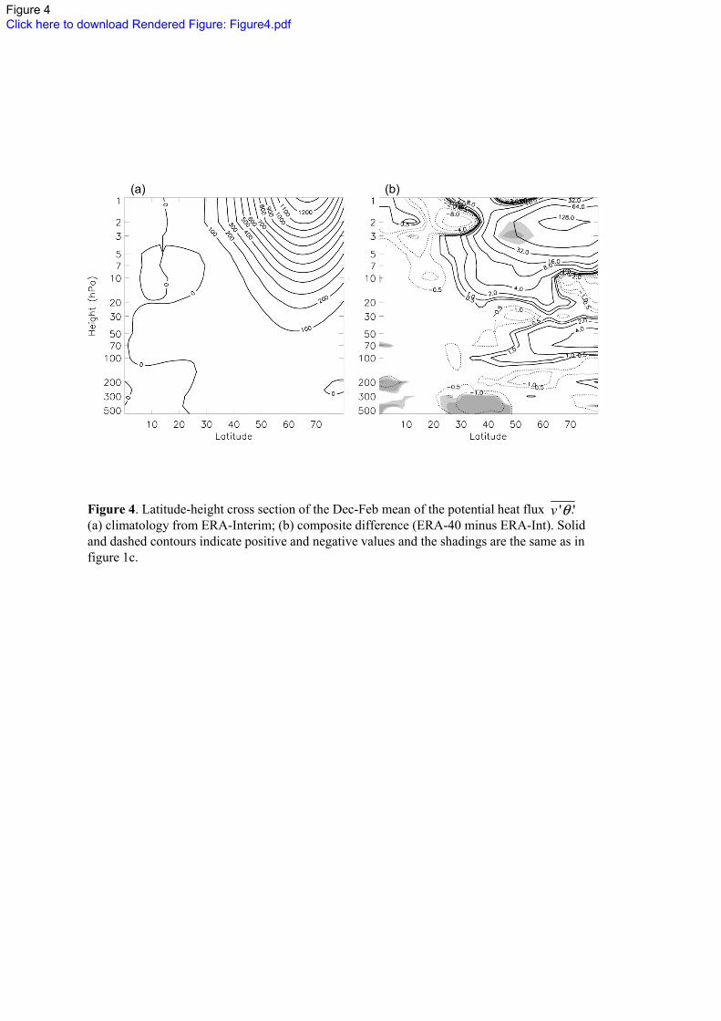
(a) (b)
Figure 4. Latitude-height cross section of the Dec-Feb mean of the potential heat flux . (a) climatology from ERA-Interim; (b) composite difference (ERA-40 minus ERA-Int). Solid and dashed contours indicate positive and negative values and the shadings are the same as in figure 1c.
' 'v θ
Figure 4Click here to download Rendered Figure: Figure4.pdf

Figure 5. Time series of Dec-Feb mean total, stationary and transient components of the zonal
mean eddy heat flux (top to bottom) averaged over 45-75N, 100hPa (left) and 10hPa (right).
The solid straight lines are the associated trends in the ERA-40 and ERA-Interim eddy heat
flux components.
year
v’T’ 4
5-7
5N
,10
0h
Pa
(K
m s
-1)
v’T’ 4
5-7
5N
,10
0h
Pa
(K
m s
-1)
v’T’ 4
5-7
5N
,10
0h
Pa
(K
m s
-1)
year
v’T’ 4
5-7
5N
,10
hP
a
(K
m s
-1)
v’T’ 4
5-7
5N
,10
hP
a
(K
m s
-1)
v’T’ 4
5-7
5N
,10
hP
a
(K
m s
-1)
12
14
16
18
20
22
1980 1985 1990 1995 2000
total
4
6
8
10
12
14
16
1980 1985 1990 1995 2000
stationary
4
6
8
10
12
14
16
1980 1985 1990 1995 2000
ERA40
ERAInt
transient
60
80
100
120
1980 1985 1990 1995 2000
total
10
30
50
70
90
1980 1985 1990 1995 2000
stationary
10
30
50
70
90
1980 1985 1990 1995 2000
ERA40
ERAInt
transient
Figure 5Click here to download Rendered Figure: Figure5.pdf
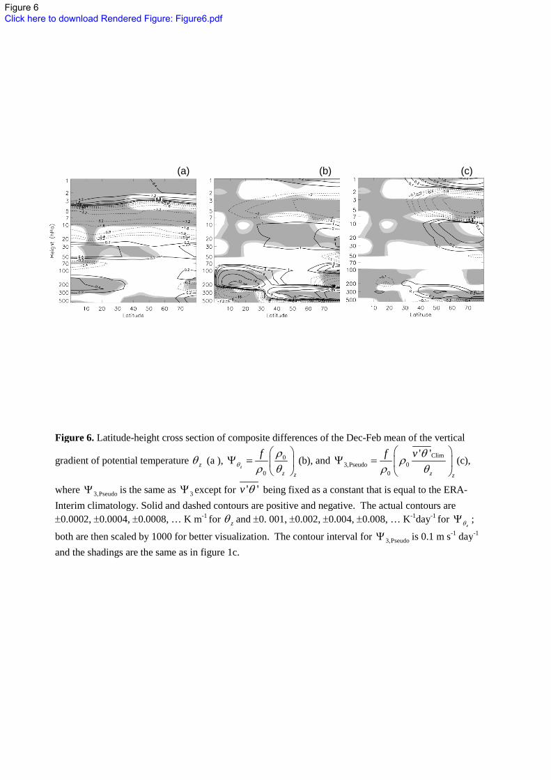
(a) (b) (c)
Figure 6 Latitude height cross section of composite differences of the Dec Feb mean of the verticalFigure 6. Latitude-height cross section of composite differences of the Dec-Feb mean of the vertical
gradient of potential temperature z (a ), 0
0z
z z
f
(b), and 3,Pseud 0o
lim
0
C' '
z z
f v
(c),
where 3,Pseudo is the same as 3 except for ' 'v being fixed as a constant that is equal to the ERA-
Interim climatology. Solid and dashed contours are positive and negative. The actual contours are 0.0002, 0.0004, 0.0008, … K m-1 for z and 0. 001, 0.002, 0.004, 0.008, … K-1day-1 for
z ;
1 1both are then scaled by 1000 for better visualization. The contour interval for 3,Pseudo is 0.1 m s-1 day-1
and the shadings are the same as in figure 1c.
Figure 6Click here to download Rendered Figure: Figure6.pdf

Figure 7. Vertical profile of the Dec-Feb zonal mean temperature (a) and the
differences between ERA-40 and ERA-Interim (b) at 0-35N, 35-75N, and 75-90N.
1
10
100
1000
-6 -4 -2 0 2 4 6
Hei
ght
(h
Pa)
TERA40ERAInt (K)
0-35N
35-75N
75-90N
1
10
100
1000
195 220 245 270 295
Hei
ght
(h
Pa)
T (K)
ERA40: 0-35N
ERA40: 35-75N
ERA40: 75-90N
ERAInt: 0-35N
ERAInt: 35-75N
ERAInt:75-90N
(a)
(b)
Figure 7Click here to download Rendered Figure: Figure7.pdf

Figure 8. Polar plot of Dec-Feb mean temperature composite differences between ERA-40 and
ERA-Interim at various pressure levels. The hatched regions indicate statistical significance at p
0.05. Note that the value range of the colour bars differs.
7hPa 20hPa
70hPa 100hPa
500hPa 850hPa
Figure 8Click here to download Rendered Figure: Figure8.pdf
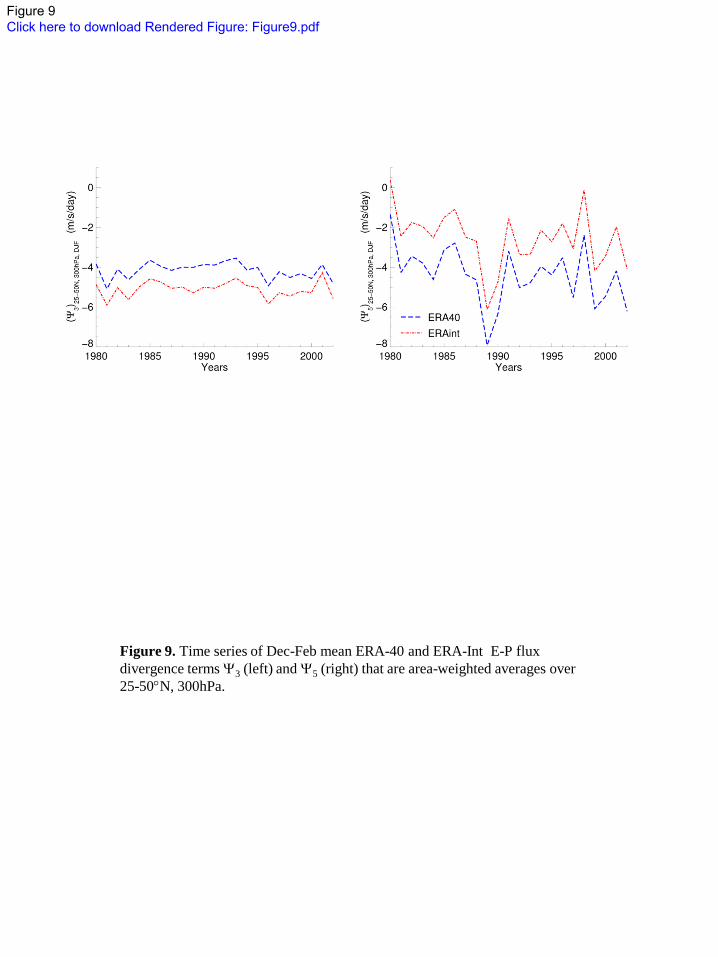
Figure 9. Time series of Dec-Feb mean ERA-40 and ERA-Int E-P flux
divergence terms 3 (left) and 5 (right) that are area-weighted averages over
25-50N, 300hPa.
Figure 9Click here to download Rendered Figure: Figure9.pdf
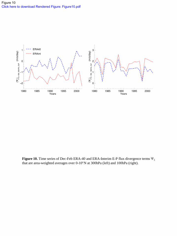
Figure 10. Time series of Dec-Feb ERA-40 and ERA-Interim E-P flux divergence terms 5
that are area-weighted averages over 0-10N at 300hPa (left) and 100hPa (right).
Figure 10Click here to download Rendered Figure: Figure10.pdf
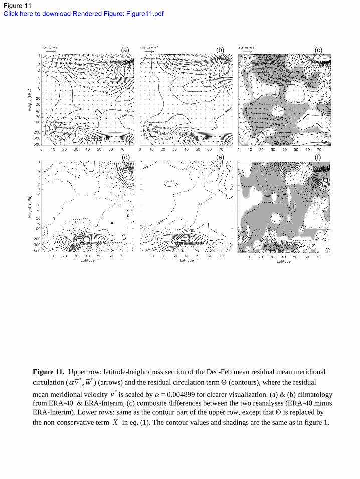
(a) (b) (c)
(d) (e) (f)
Figure 11. Upper row: latitude-height cross section of the Dec-Feb mean residual mean meridional
circulation (* *,v w ) (arrows) and the residual circulation term (contours), where the residual
mean meridional velocity *v is scaled by = 0.004899 for clearer visualization. (a) & (b) climatology
from ERA-40 & ERA-Interim, (c) composite differences between the two reanalyses (ERA-40 minus
ERA-Interim). Lower rows: same as the contour part of the upper row, except that is replaced by
the non-conservative term X in eq. (1). The contour values and shadings are the same as in figure 1.
Figure 11Click here to download Rendered Figure: Figure11.pdf
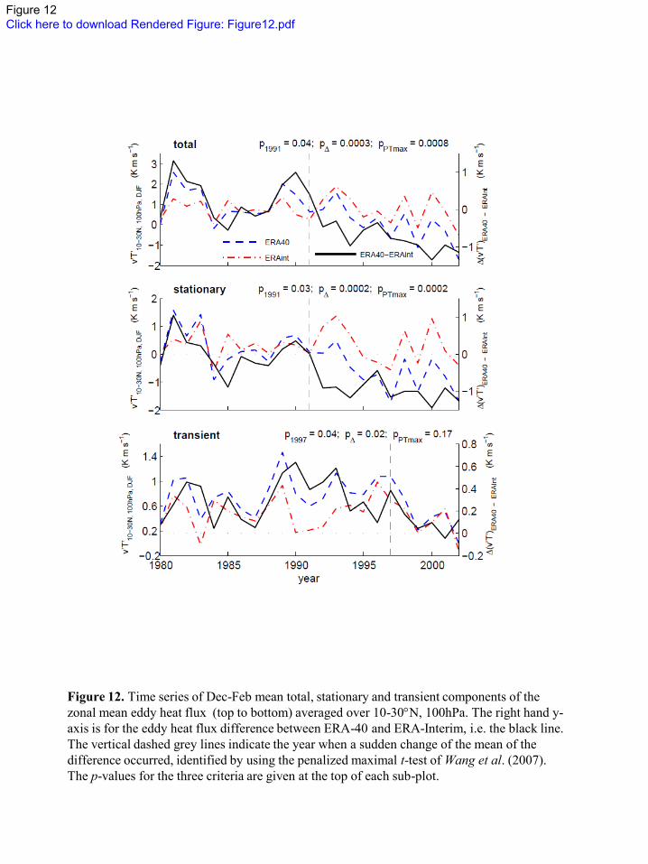
Figure 12. Time series of Dec-Feb mean total, stationary and transient components of the
zonal mean eddy heat flux (top to bottom) averaged over 10-30N, 100hPa. The right hand y-
axis is for the eddy heat flux difference between ERA-40 and ERA-Interim, i.e. the black line.
The vertical dashed grey lines indicate the year when a sudden change of the mean of the
difference occurred, identified by using the penalized maximal t-test of Wang et al. (2007).
The p-values for the three criteria are given at the top of each sub-plot.
Figure 12Click here to download Rendered Figure: Figure12.pdf
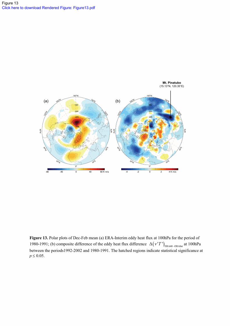
150o W 150 oE
180oW
150o W 150 oE
180oW
(a) (b)
Mt. Pinatubo(15.13°N, 120.35°E)
120
o W
90oW
90o E
120 oE
15N
30N
45N
60N
75N
120
o W
90oW
90o E
120 oE
15N
30N
45N
60N
75N
( ) ( )
60 oW
30 oW
0o
30o E
60
o E
-80 -40 0 40 80 K m/s
60 oW
30 oW
0o
30o E
60
o E
-4 -2 0 2 4 K m/s
Figure 13. Polar plots of Dec-Feb mean (a) ERA-Interim eddy heat flux at 100hPa for the period of
1980-1991; (b) composite difference of the eddy heat flux difference ERA40 -ERAInt' 'v T at 100hPa
between the periods1992-2002 and 1980-1991. The hatched regions indicate statistical significance at p 0.05.
Figure 13Click here to download Rendered Figure: Figure13.pdf

Figure 14. Same as figure 12 except for the averaged eddy head flux at 45-75N, 10hPa.
Figure 14Click here to download Rendered Figure: Figure14.pdf

150o W 150 oE
180oW
15N
150o W 150 oE
180oW
15N(a) (b)
120
o W
90oW
60 oW 60o E
90o E
120 oE
30N
45N
60N
75N
120
o W
90oW
60 oW 60o E
90o E
120 oE
30N
45N
60N
75N
W
30 oW
0o
30o E
6
-180 -120 -60 0 60 120 180 K m/s
W
30 oW
0o
30o E
6
-30 -20 -10 0 10 20 30 K m/s
Figure 15. Same as figure 13 except for at 10hPa and with a changepoint in 1998.
Figure 15Click here to download Rendered Figure: Figure15.pdf