,- _'/._.... 205841

Intraseasonal and lnterannual Variabilityof Mars' Present Climate

//j ,,,t-,/_

A NASA Ames Research Center Joint Research Interchange

Final Report

Jeffery L Hollingsworth "t, Alison F. C. Bridger _ & Robert M. Haberle t

University Consortium Agreement: NCC2-5094

Project Duration: 25 August 1994-24 February 1996

"San Jose State University Founda_on, P.O. Box 720130, San Jo._'..Selifomia 95172, USAtNASA Ames Research Center, MS: 245-3, Moflett Field, California 94035, USA

bDepartment of Meteorology, San Jose State University, San Jose, California 95192, USA

ABSTRACT

This is a Final Report for a Joint Research Interchange (JRI) between NASA Ames ResearchCenter and San Jose State University, Department of Meteorology. The focus of this JRI has

been to investigate the nature of intraseasonal and interannual variability of Mars' present cli-

mate. We have applied a three-dimensional climate model based on the full hydrostatic prim-itive equations to determine the spatial, but primarily, the temporal structures of the planet's

large-scale circulation as it evolves during a given seasonal advance, and, over multi-annual

cycles. The particular climate model applies simplified physical parameterizations and is com-putationally effbient. It could thus easily be integrated in a perpetual season or advancing

season configuration, as well as over many Mars years. We have assessed both high andlow-frequency components of the circulation (i.e., motions having periods of (..0(2-10 days) or

greater than O(10 days), respectively). Results from this investigation have explored the basicissue whether Mars' climate system is naturally 'chaotic' associated with nonlinear interactions

of the large-scale circulation--regardless of any allowance for ye" t-to-year variations in exter-nal forcing mechanisms. Titles of papers presented at scientific conferences and a manuscript

to be submitted to the scientific literature are provided. An overview of a areas for further in-vestigation is also presented.

1. INTRODUCTION

Fluctuations in a planet's atmospheric circulation are either internal in nature, caused by in-trinsic instability of the flow and by interactions between different types of motions; or exter-

nal in origin, caused by variations in imposed external parameters (e.g., variations in incident

solar radiation with a planet's orbit or coupling between surface fields (e.g., topography, polarice caps) and the atmosphere [1,2]. Fundamental questions related to a planet's climate are:

Which process is responsible for the strongest long-period variability? And, what is the natureof the interactions between the two kinds of fluctuations?

Hollingsworth et al. 2

Over a range of spatial and temporal scales, Mars' atmosphere, as Earth's, exhibits sub-

stantial variations in its field variables (e.g., temperature and momentum) and trace constituents

(e.g., water vapor and dust). The spatial and temporal variations can be associated with awide variety of intemal and extemaJ physical processes within its atmosphere [3,4]. Analyses of

Vildng lander surface-pressure data have indicated definitive evidence for specific meteorolog-ical signals such as thermal tides [5] and recurrent midlatitude weather systems (i.e., transient

baroclinic eddies) [6,7]. However a complete observational database of global meteorologi-

cal variables, in particular their variations during a seasonal cycle and from year-to-year, doesnot presently exist for Mars. One must therefore resort to other means to infer aspects of theplanet's global circulation patterns and climate. One such method is the application of atmo-

spheric dynamical models.

By far the most sophisticated models are general circulation models (GCMs). These mod-els include detailed formulations of atmospheric flow dynamics based on the meteorological

primitive equations; they also include complex physics for 'right hand side' terms ;n the govern-

ing system of equations (e.g., radiative-transfer physics to yield diabatic heati_,g rates). GCMs

are thus computationally intensive. Another approach is to simplify the physics without compro-

mising the flow dynamics. This is a so called 'simple physics' primitive equations (SPPE) model.SPPE models are efficient 'mechanistic' tools that can be used to examine particular compo-

nents of the atmospheric circulation (e.g., the zonally symmetric circulation, the transient circu-lation and the stationary circulation) and their mutual interactions. They are also useful in per-

forming parameter sensitivity studies (e.g., determining the sensitivity to thermal relaxation andmomentum dissipation strengths). And because computations related to the extemaJ physics

are minimized, SPPE models are effective numerical models for performing multi-annual sim-

ulations which can be used to address questions related to long-term intemally or externallydriven climate variability.

We have adapted the SPPE model of [8] to investigate aspects of Mars' atmospheric cir-

culation and the nature of its present climate. The Mars climate model (MCM) uses simplifiedphysical parameterizations: diabatic heating is specified in terms of a meridionally dependent

thermal relaxation (Newtonian cooling) towards a 'radiative-equilibrium' temperature field, andmomentum drag is specified in terms of a height-dependent drag (Rayleigh friction). A pre-

scribed zonally symmetric radiative-equilibrium thermal field as a function of latitude, heightand season is independently determined using results from a 1-D radiative-convective model.

The MCM uses a spectral (spherical harmonic) representation in the horizontal and finite differ-

ences in the vertical for computations of the dependent variables. The seasonal condensationof CO_ onto the polar caps is also included with a parameterization.

The MCM has been used successfully to investigate key components of Mars' atmospheric

circulation, for example, its zonally symmetric (Hadley) circulation and its midlatitude thermally

indirect (Fen'el) circulation [9]. Driven by large-scale traveling weather systems (i.e., transientbarotropic and/or baroclinic eddies) which grow and decay within the rapidly rotating, intrinsi-

cally unstable atmosphere, this latter extratropicaJ circulation is a key agent in the transport

of heat and momentum [10] and particular to Mars, volatiles and dust [4]. In many aspects,the MCM shows qualitatively and quantitatively similar structures of the global circulation as

in the fully complex Mars general circulation model (MGCM) used at NASA Ames [11,12,13].

Yet because of its simple physics parameterizations, the MCM is more ideally suited to performmulti-annual simulations aimed at addressing questions related to internally or externally driven

variability of Mars' long-term climate.

Hollingsworthel at, 3

2. KEY RESULTS OF INVESTIGATION

The pdmary objectives of this research were: (a) to examine both high and low-frequencyspatial and temporal structures of mean and eddy statistics from simulations of Mars' atmo-

spheric circulation; and, (b) to examine the degree and significance of intraseasonal and in-

terannual (i.e., ultra-low frequency) variability of the planet's current climate. Both objectiveswere addressed using the computationally effi;ient, three-dimensional Mars climate model de

scdbed above. By 'high', 'low' and 'ultra-low' frequency, it is meant atmospheric circulation com-

ponents with periods of O(2-10 days), O(10-100 days) and O(1-10 years), respectively. By

'mean' and 'eddy' it is meant a time and/or zonal average, and the departures therefrom. By'intraseasonal' and 'interannual' variability it is meant significant circulation changes within a

given seasonal progression (e.g., fall through spring in the northem hemisphere) and varia-tions in such changes from year-to-year, and significant year-to-year departures of particular

mean and eddy statistics of the circulation, respectively.

a. Multi-annual simulations: interannual variability

A total of 60 Mars years in a 'coarse' configuration (i.e., 'trapezoidal' spherical harmonictruncation 16Tr06 and 14 vertical layers) with no topography nor CO2 condensation cycle have

been simulated using the MCM. From such a long integration, a realistic data set has been pro-duced to investigate variability of the circulation and climate on intraseasonaJ and interannual

time scales. Absence of complex extemal forcings (e.g., realistic solar/IR radiation and sur-

face variations) permits intemally generated (i.e., nonlinear) variability of the climate system tobe examined in isolation. The predominant extemal forcing in this version of the MCM is the

radiative relaxation applied to drive the climate through its annual cycle. It also imposes the

longest time scale on the system. Any variability seen on longer time scales is thus generatedintemally.

Even in the absence of realistic extemal forcings (e.g., enhanced thermal radiation ac-

companying high dust loading or large-scale flow interaction with spatially varying surface to-pography), the long-term simulation has indicated significant interannual variability, with the

greatest variations occurring in the southem hemisphere (SH) during late winter and spring sea-

sons. The variability of the circulation has been assessed by examination of hemisphericallyintegrated zonal and eddy kinetic energies (ZKE and EKE, respectively [14]).

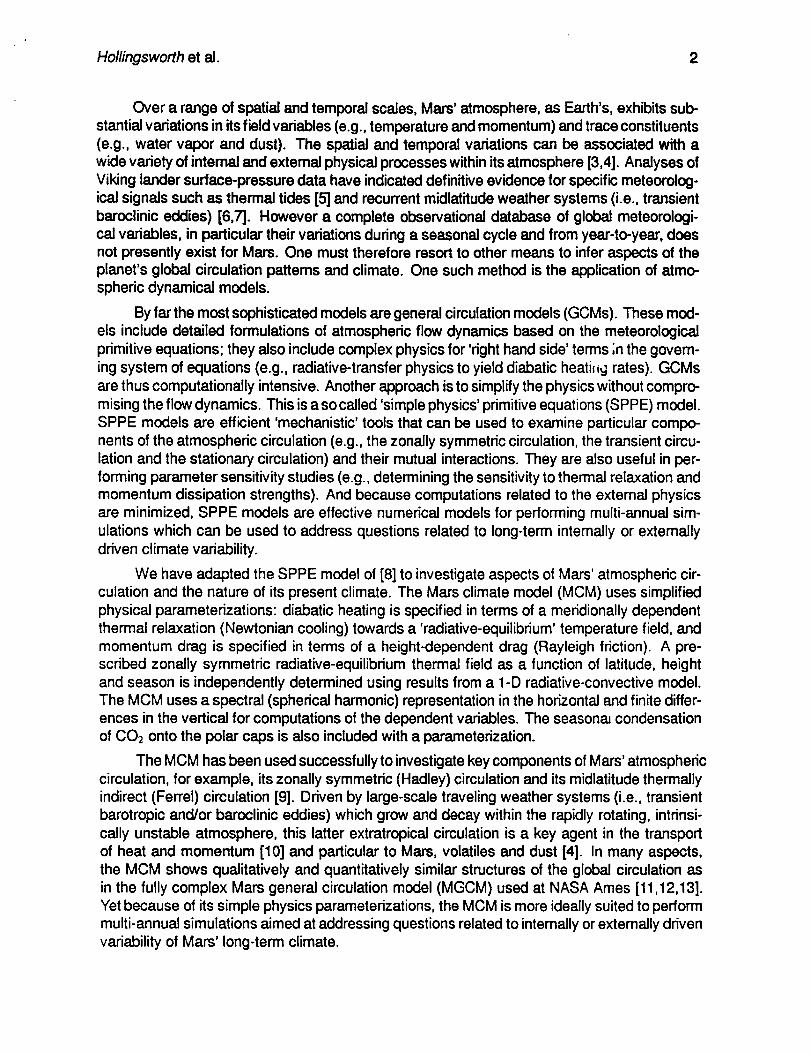
Figure 1 shows an example of year-to-year variations in the northem hemisphere (NH)

mean zonal kinetic energy as a function of season for the first 10 years of the 60 year simulation.

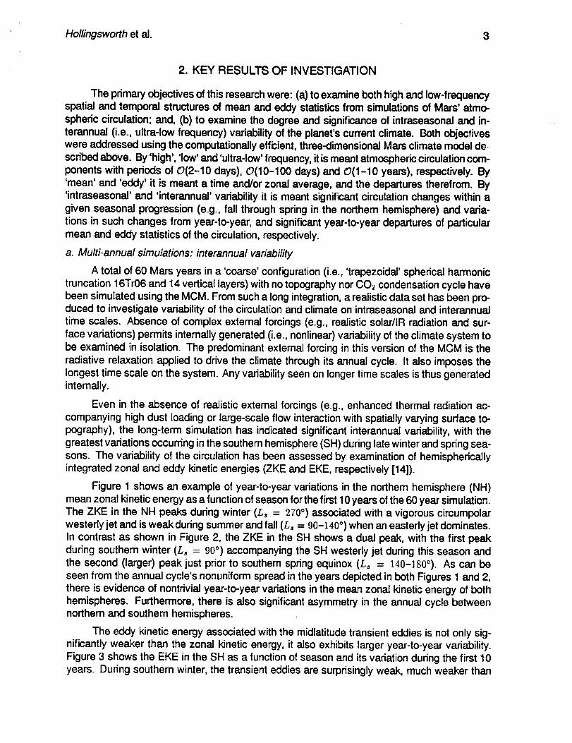
The ZKE in the NH peaks during winter (/_,, = 270 °) associated with a vigorous circumpolarwesterly jet and is weak during summer and fall (/_,, = 90-140 °) when an eastedy jet dominates.In contrast as shown in Figure 2, the ZKE in the SH shows a dual peak, with the first peak

during southem winter (Ls = 90 °) accompanying the SH westerly jet during this season and

the second (larger) peak just prior to southern spring equinox (Ls = 140-]80°). As can be

seen from the annual cycle's nonuniform spread in the years depicted in both Figures 1 and 2,there is evidence of nontrivial year-to-year variations in the mean zonal kinetic energy of both

hemispheres. Furthermore, there is also significant asymmetry in the annual cycle betweennorthem and southern hemispheres.

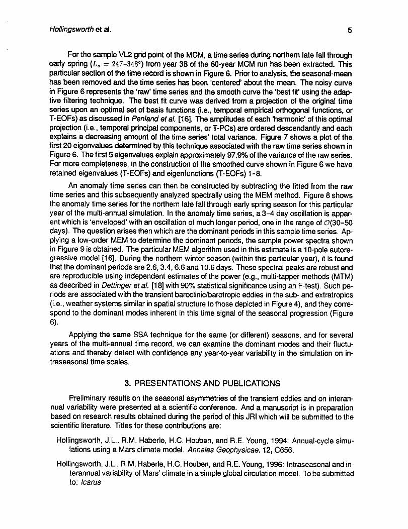
The eddy kinetic energy associated with the midlatitude transient eddies is not only sig-

nificantly weaker than the zonal kinetic energy, it also exhibits larger year-to-year variability.Figure 3 shows the EKE in the SH as a function of season and its variation during the first 10

years. During southern winter, the transient eddies are surprisingly weak, much weaker than

Hollingsworthelal. 4

their counterparts during northem winter. Similar weak transient-eddy activity has been foundin the NASA Ames MGCM [13]. It appears that the weak activity is, in part, independent of

the details of zonally symmetric or asymmetric surface forcings (e.g., large-scale topography).Other intemal processes must be important. However, SH eddy activity rises dramatically dur-

ing spring and is far greater than that in the north at any season. A similar seasonal pattemas seen in Figure 3 is apparent for the NH transient eddies yet the fluctuations are much less

pronounced. This year-to-year variability in SH winter transient eddy activity occurs in a model

with simple but repeatable forcing. And it therefore suggests that Mars' climate system hassufficient nonlinearity to produce interannual variability regardless of specific details of the im-posed extemal forcing.

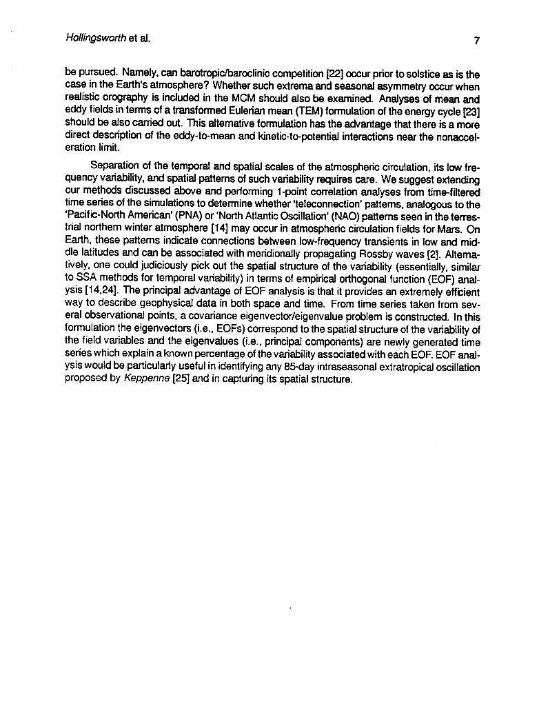
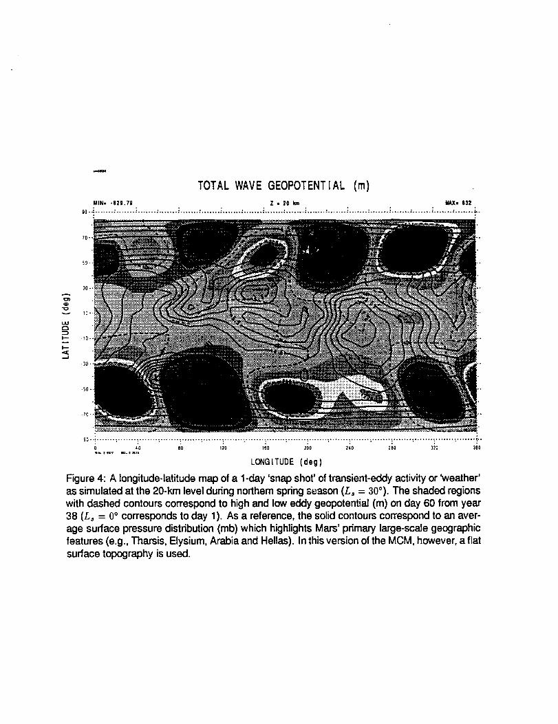
A 1-day 'snap shot' of the transient-eddy activity or 'weather' as simulated by the MCM

is indicated in Figure 4. The particular season chosen corresponds to northem spring where

eddies are active in both hemispheres. At this level in the atmosphere (roughly 20 km), theeddy geopotential shows a series of high and low centers in the middle latitudes with a dominant

wavenumber-3 pattem. The latitudinal band of the centers of these weather systems (i.e., :1:50-

60° ) corresponds to active 'storm belts' [15] on Mars during this season.

We have also examined time series from the MCM grid point nearest the Viking Lander

2 (VL2) site for long-term variability (in the present model configuration, this is at 126 deg E,

47 deg N, 0.3 km). As seen in Figure 5, the 60-year record of once daily (instantaneous) tem-perature shows a 'red noise' spectrum characteristic of geophysical time series, with a marked

increase in spectral power toward the lowest frequencies [1,16] here, out to the decadal time

scales. The annual, semi-annual and sub-annual harmonics exhibit the greatest power, and

a hint of variability on time-scales larger than the annual-cycle can also be seen. Moreover,considerable variability in the 10-100 day range and 2-0 day range is apparent, which is as-

sociated with low-frequency wave activity on intraseasonai time scales [15] and the passage

of developing and decaying weather cyclones (i.e., day-to-day fluctuations), respectively, overthe sample grid point. The latter eddy activity occurs in the midlatitude storm belt mentioned

earlier and can be highly modulated by the presence of Mars' continental-scale orography [17].

Such effects are not present in the current version of the MCM. The low-frequency variations ofthe atmospheric circulation are not present merely at this particular grid point. Sample powerspectra of a daily time series constructed by vertically integrating the mean equator-to-pole tem-

perature difference exhibit very similar dominant spectral peaks and variability.

b. Multi-annual simulations: intraseasonal variability

In order to systematically analyze any 'noisy' circulation time series produced by the MCM,and the statistical significance of the results, we have applied useful analysis tools originally de-

veloped for Earth atmospheric studies to the climate model. Singular spectrum analysis (SSA)

has been used to improve the determination of spectral estimates and to isolate statisticallysignificant spectral power [16,18]. Essentially, SSA is an optimal-adaptive filtering technique;when used in combination with low-order maximum entropy (i.e., autoregressive) models (MEM),

SSA is very effective in isolating dominant periods of motions when the background noise maybe 'white' [16].

To assess, for example, the dominant periods of motion in the circulation over an intrasea-

sonal time scale, and moreover, any significant variability in such periods from year to year, SSAcan be used on a subset of a multi-year time series. Below we demonstrate the technique usinga time series from the climate model multi-annual simulation.

Hollingsworthelai. 5

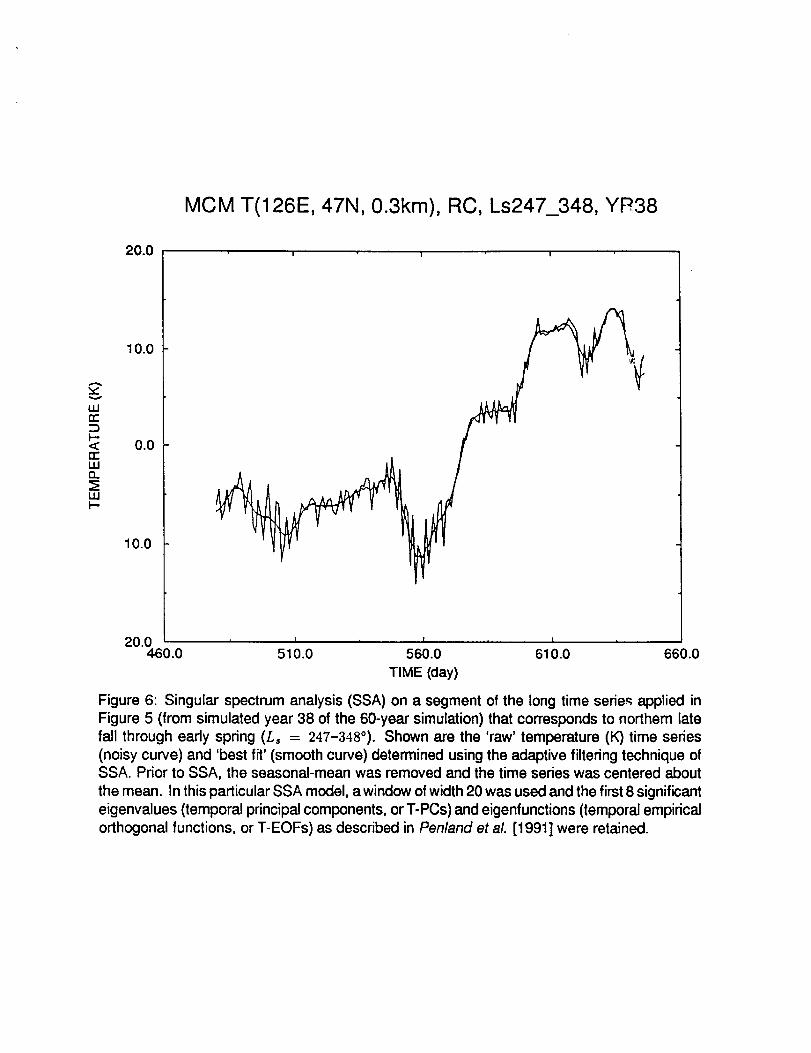
For the sample VL2 grid point of the MCM, a time series during northem late fail throughearly spring (Ls = 24?-348 °) from year 38 of the 60-year MCM run has been extracted. This

particular section of the time record is shown in Figure 6. Prior to analysis, the seasonal-mean

has been removed and the time series has been 'centered' about the mean. The noisy curve

in Figure 6 represents the 'raw' time series and the smooth curve the 'best fit' using the adap-

tive filtering technique. The best fit curve was derived from a projection of the original timeseries upon an optimal set of basis functions (i.e., temporal empirical orthogonai functions, orT-EOFs) as discussed in Penland et al. [16]. The amplitudes of each 'harmonic' of this optimal

projection (i.e., temporal principal components, or T-PCs) are ordered descendantly and eachexplains a decreasing amount of the time series' total variance. Figure 7 shows a plot of the

first 20 eigenvaJues determined by this technique associated with the raw time series shown inFigure 6. The first 5 eigenvaJues explain approximately 97.9% of the variance of the raw series.

For more completeness, in the construction of the smoothed curve shown in Figure 6 we have

retained eigenvalues (T-EOFs) and eigenfunctions (T-EOFs) 1-8.

An anomaly time series can then be constructed by subtracting the fitted from the rawtime series and this subsequently analyzed spectrally using the MEM method. Figure 8 shows

the anomaly time series for the northern late fall through early spring season for this particular

year of the multi-annual simulation. In the anomaly time series, a 3-4 day oscillation is appar-ent which is 'enveloped' with an oscillation of much longer period, one in the range of 0(30-50

days). The question arises then which are the dominant periods in this sample time series. Ap-plying a low-order MEM to determine the dominant periods, the sample power spectra shown

in Figure 9 is obtained. The particular MEM algorithm used in this estimate is a 10-pole autore-gressive model [16]. During the nor'them winter season (within this particular year), it is foundthat the dominant periods are 2.6, 3.4, 6.6 and 10.6 days. These spectral peaks are robust and

are reproducible using independent estimates of the power (e.g., multi-tapper methods (MTM)

as described in Dettinger et aL [18] with 90% statistical significance using an F-test). Such pe-riods are associated with the transient baroclinic/barotropic eddies in the sub- and extratropics

(i.e., weather systems similar in spatial structure to those depicted in Figure 4), and they corre-

spond to the dominant modes inherent in this time signal of the seasonal progression (Figure6).

Applying the same SSA technique for the same (or different) seasons, and for severalyears of the multi-annual time record, we can examine the dominant modes and their fluctu-

ations and thereby detect with confidence any year-to-year variability in the simulation on in-traseasonai time scales.

3. PRESENTATIONS AND PUBLICATIONS

Preliminary results on the seasonal asymmetries of the transient eddies and on interan-

nual variability were presented at a scientific conference. And a manuscript is in preparation

based on research results obtained during the period of this JRI which will be submitted to thescientific literature. Titles for these contributions are:

Hollingsworth, J.L., R.M. Haberle, H.C. Houben, and R.E. Young, 1994: Annuai-cycle simu-

lations using a Mars climate model. Annales Geophysicae, 12, C656.

Hollingsworth, J.L., R.M. Haberle, H.C. Houben, and R.E. Young, 1996: Intraseasonai and in-

terannual variability of Mars' climate in a simple global circulation model. To be submittedto: Icarus

Hollingsworthet al. 6

4. DISCUSSION AND AREAS FOR FUTURE WORK

Understanding the dynamical mechanisms responsible for the rise and fall of the transient

eddy activity during seasonal advance, the hemispheric asymmetries in mean and eddy ener-getics of the circulation, the sensitivity to realistic albeit mechanistic extemal forcings, and the

influences each has on the intraseasonal and interannual variability of Mars' climate are top-ics we have begun to investigate under this research agreement. We have, nevertheless, onlyanalyzed a small subset of our long-time record from the 60-year simulation. We outline below

areas for further investigation related to intraseasonal variability for other pedods, variabilitYunder enhanced dust Ioadings, and other potential measures of interannual variability.

a. Multi-annual simulations: enhanced dust opacities and imposed dust cycle

Isolating fundamental causes of Mars' climate variability while the 'system' (i.e., atmo-

sphere and surface interface) is forced at the annual frequency under both low and quasi-periodic

enhanced dust Ioadings, could be examined mechanistically with the coupled MCM. Thoughthere is ample evidence that a preferred seasonality exists when planet-encircling storms are

generated, it is recognized that the global storms occur intermittently on a year-to-year basis[19]. Ingersoll and Lyons [20] argued using a simplified two-parameter dust-circulation model

that a possible source for interannual variability is the dust loading itself (i.e., an extemal forc-ing). Assuming equal time scales for dust raising and dust storm decay, aperiodic solutions

were found for a wide range of parameter choices. Whether realistic Mars climate models such

as the MCM show naturally 'chaotic' solutions in multi-annual simulations, without year-to-yearvariations in external forcings (e.g., regional versus global atmospheric dustiness), should be

investigated. Chaotic signatures (i.e., 'red' power spectra) may arise solely associated with thenonlinearity of the goveming flow equations. Yet it may also be associated with interactions be-

tween a forced, steady circulation and the life cycles of the transient eddies [1,21].

Long-term perpetual-season, as well as multi-annual simulations should be performedwith a modified version of the MCM that incorporates realistic large-scale surface topography.

The experiments performed to date do not include topographic effects. Originally, we had plannedto include topography in the MCM; however, the required code modifications and necessarymodel testing proved to be formidable. Under this agreement, we therefore decided to exam-

ine long-term circulation statistics using the simpler lower boundary condition exclusively. Con-

ceivably, 60-100 years of time integration should be performed with a topography version of theMCM in order to detect with confidence the low-frequency, annual and decadal time-scale vari-

ability in these simulations. A small suite of simulations will be carded out for the annual-cyclehaving

• idealized topography (i.e., hemispherically isolated mountains)

• a COs condensation cycle

• enhanced dust loading (i.e., dusty radiative equilibrium temperatures and relaxation rates)

• a Viking Lander-like dust opacity cycle

b. Low-frequency variability: spatial structures

Further investigation on the dynamical mechanisms responsible for the relative minimumfound in the integrated EKE near winter solstice in the simulations without topography should

I-Iollingsworth et al. 7

be pursued. Namely, can barotropic/baroclinic competition [22] occur prior to solstice as is the

case in the Earth's atmosphere? Whether such extrema and seasonal asymmetry occur when

realistic orography is included in the MCM should also be examined. Analyses of mean and

eddy fields in terms of a transformed Eulerian mean (TEM) formulation of the energy cycle [23]should be also carried out. This altemative formulation has the advantage that there is a more

direct description of the eddy-to-mean and kinetic-to-potential interactions near the nonaccel-eration limit.

Separation of the temporal and spatial scales of the atmospheric circulation, its low fre-

quency variability, and spatial pattems of such variability requires care. We suggest extendingour methods discussed above and performing 1-point correlation analyses from time-filtered

time series of the simulations to determine whether 'teleconnection' pattems, analogous to the'Pacific-North American' (PNA) or 'North Atlantic Oscillation' (NAO) pattems seen in the terres-trial northem winter atmosphere [14] may occur in atmospheric circulation fields for Mars. On

Earth, these pattems indicate connections between low-frequency transients in low and mid-

dle latitudes and can be associated with meridionally propagating Rossby waves [2]. Altema-

tively, one could judiciously pick out the spatial structure of the variability (essentially, similarto SSA methods for temporal variability) in terms of empirical orthogonal function (EOF) anal-

ysis [14,24]. The principal advantage of EOF analysis is that it provides an extremely effcientway to describe geophysical data in both space and time. From time series taken from sev-

eral observational points, a covariance eigenvector/eigenvalue problem is constructed. In this

formulation the eigenvectors (i.e., EC)Fs) correspond to the spatial structure of the variability ofthe field variables and the eigenvalues (i.e., principal components) are newly generated timeseries which explain a known percentage of the variability associated with each EOF. EOF anal-

ysis would be particularly useful in identifying any 85-day intraseasonal extratropicaJ oscillationproposed by Keppenne [25] and in capturing its spatial structure.

Hollingsworthetal. 8

REFERENCES

1. James, I. N., and P. M. James, 1992: Quart. J. Roy. Meteor. Soc., 118, 1211-1233.

2. James, I. N., 1994: Introduction to Circulating Atmospheres, (Cambridge Univ. Press., Cam-

bddge).

_. Leovy, C. B., 1985: Adv. Geophys. 28, Part A, 327-346.

4. Zurek, R. W., et al., 1992: in Mars, H. H. Kieffer, B. M. Jakosky, C. W. Snyder, and M. S.Matthews, Eds., (Univ. Adzona Press, Tucson), 835-933.

5. Leovy, C. B., and R. W. Zurek, 1979: J. Geophys. Res., 84, 2956-2968.

6. Barnes, J. R., 1980: J. Atmos. ScL, 37, 2002-2015.

7. Barnes, J. R., 1981: J. Atmos. Sci., 38, 225-234.

8. Young, R. E. and G. L Villere, 1985: J. Atmos. Sci., 42, 1991-2006.

9. Haberle, R. M., H. Houben, R. E. Young, and J. R. Barnes, 1996: (Submitted to J. Geophys.

Res.).

10. Hoskins, B. J., et al., 1983: J. Atmos. Sci., 40, 1595-1612.

11. Pollack, J. B., et al., 1990: J. Geophys. Res., 95, 1447-1474.

12. Haberle, R. M., et al., 1993: J. Geophys. Res., 98, 3093-3124.

13. Barnes, J. R., et al., 1993: J. Geophys. Res., 98, 3125-3148.

14. Peixoto, J. P., and A. H. Oort, 1992: Physics of Climate, (American Institute of Physics,New York).

15. Grotjahn, R., 1993: Global Atmospheric Circulations: Observations and Theories, (Oxford

Univ. Press, New York).

16. Penland, C., M. Ghil, and K. M. Weickmann, 1991: J. Geophys. Res., 96, 22659-22671.

17. Hollingsworth, J. L., et al., 1996: Nature, 380, 413-416.

18. Dettinger, M. D., et al., 1995: Eos, Trans. American Geophysical Union, 76, 12, 14, 21.

19. Zurek, R. W., and L J. Martin, 1993: J. Geophys. Res., 98, 3247-3259.

20. Ingersoll, A. P., and J. R. Lyons, 1993: J. Geophys. Res., 98, 10951-10961.

21. James, P. M., I. N. James and K. Fraedrich, 1994: Quart. J. Roy. Meteor. Soc., 120, 1045-1067.

22. James, I. N., 1987: J. Atmos. ScL, 44, 3710-3720.

23. Plumb, R. A., 1983: J. Atmos. Sci., 40, 1669-1688.

24. Horel, J. D., 1981: Mon. Wea. Rev., 109, 2080-2092.

25. Keppenne, C. L., 1992: Icarus, 100, 598-607.

E

,-!

ILl

N

9008800750700650600550500450400350300250200150100

500

MIN= 21.505

NH K INE T I C ENERGY

5O

MAX= 663.12

0 90 180 270 360

Ls (degs)

Figure 1: Vertically and hemispherically averaged mean zonal kinetic energy (m2 s -2) as a

function of season (Ls) for the northern hemisphere for the first 10 years of a 60-year simu-lation with the Mars climate model (MCM). The zonal kinetic energy (ZKE) is computed from

the instantane,:;us (once daily), longitudinally averaged horizontal wind components (i.e., north-south, east-west) at all model levels.

E

uJ

1",4

MIN= 22.1

O05O-00:50-00-50:00-50-O0Z50-"00:50 =00=50- _'

oo:/5000-

50-

0

SH KINETI C ENERGYMAX. 683.8

L

L

L

L

L

0 90 180 270

Ls (degs)360

Figure 2: As in Figure 1 but for the southem hemisphere.

E

LLi

UJ

200

150

100

50

MIN= 4.2217

SH K/NETIC ENERGYMAX- 203.82

0 90 180 270 360

L_ (degs)

Figure 3: As in Figure 2 but for the vertically and hemispherically averaged transient-eddy ki-netic energy (m 2 s-2). The eddy kinetic energy (EKE) is computed from the instantaneous de-

partures (once dally) of the horizontal wind components (i.e., north-south, east-west) from thezonal (longitudinal) means at all model levels.

,,L14m_

TOTAL WAVE GEOPOTENTIAL (m)

MIN- -829.79 Z • 20 km MAX- 632

90-_ ....... : ....... "....... : ....... "....... : ....... -:....... : ....... "....... : ....... i ....... ."....... "....... ."....... .:....... : ....... _....... ."....... "L.

70-

-lC • -:

go-._ ....... : ....... •....... : ....... • ....... : ....... _....... : ....... _....... : ....... _........ : ....... • ....... : ....... ! ....... ......... -0 40 B0 120 t60 200 240 280 320 360

LONGITUDE (deg)

Figure 4: A longitude-latitude map of a 1-day 'snap shot' of transient-eddy activity or 'weather'

as simulated at the 20-kin level during northern spring s_ason (L, = 30°). "The shaded regions

with dashed contours correspond to high and low eddy geopotential (m) on day 60 from year38 (Ls = 0° corresponds to day 1). As a reference, the solid contours correspond to an aver-

age surface pressure distribution (mb) which highlights Mars' primary large-scale geographic

features (e.g., Tharsis, Elysium, Arabia and Hellas). In this version of the MCM, however, a flat

surface topography is used.

MCM

106

_. 10s-:>,,=

-o 104 -

" 310 -

V

102 -UJ

_ 10 _ -!---

_ 0a. 10 -

_ 10 "_-

a_ 1(i.2_

10 .3

T ( 126E, 47N, O.3km) : ANN CYC + ANOMALYMAX= 5. 8242

I I I I

I I I

10s 104 103 102 101 100

PERIOD (days)

Figure 5: Band-averaged power density spectrum (IG day) computed from a 60-year temper-ature time series (sampled once daily) from the MCM grid point nearest the Viking Lander 2

(VL2) site. (For the multi-year integrations in the specified model resolution, this grid point cor-responds to 126 ° E, 47 ° N, and 0.3 kin.) Prior to application of the FFT, the time series was band

averaged into bins having a width of 5 days. The 90% confidence limits on the band-averagedspectral estimates using a Chi-square distribution and 10 degrees of freedom is indicated bythe error bar.

MCM T(126E, 47N, 0.3km), RC, Ls247_348, YP38

20.0I i I

-,e"

LLIn-

t--<I:n"LLI13.

LUI--

10.0

0.0

10.0

20.0 , i , t , I ,460.0 510.0 560.0 610.0 660.0

TIME (day)

Figure 6: Singular spectrum analysis (SSA) on a segment of the long time sede_ applied in

Figure 5 (from simulated year 38 of the 60-year simulation) that corresponds to northern latefall through early spring (Ls = 247-348°). Shown are the 'raw' temperature (K) time series

(noisy curve) and 'best fit' (smooth curve) determined using the adaptive filtering technique ofSSA. Prior to SSA, the seasonal-mean was removed and the time series was centered about

the mean. In this particular SSA model, awindow of width 20 was used and the first 8 significant

eigenvalues (temporal principal components, or T-PCs) and eigenfunctions (temporal empirical

orthogonal functions, or T-EOFs) as described in Penland et al. [1991] were retained.

ILl:ED_-I

ZLL!

I

LL.I

107

106 -

105 -

104 -

103 -

102 -

101 -

100 -

10-1 -

10-2 -

10 .30

SSA (MCM T, Ls247_348, YR38)MIN= 0 MAX= 0

.... I , , , , I .... I , , , I I , , J , I , , , ,

' ' ' ' I ' ' ' ' I ' ' ' ' I ' ' ' ' I ' ' ' ' I ' ' ' '

5 10 15 20 25

EIGENVALUE INDEX (N-D)

30

Figure 7: The first 20 eigenvalues of the centered raw time series shown in Figure 6. Eigen-values 1-5 explain 97.9% of the variance.

MCM T(126E, 47N, 0.3km), ANOM, Ls247_348, YR38

4.0I I I

v

Wrr

I--<n"WQ.

uJI--

2.0

0.0

2.0

V

40. , I , I , I J

460.0 510.0 560.0 610.0 660.0

TIME (day)

Figure 8: The 'anomaly' temperature (K) time series formed by subtracting the best fit from theraw time series shown in Figure 6.

101

MEM (MCM T ANOM, Ls247_348, YR38)

100

ZIJJa,_]< 101rr

ouJn0_n-UJ

• 10_-0Q.

1 0 3 , I , I , I , I ,

0.00 0.10 0.20 0.30 0.40 0.50

FREQUENCY (1/day)

Figure 9: Power spectral density estimates from the maximum entropy method (MEM) using 10poles in the autoregressive (AR) model [Pen�and eta/., 1991] of the anomaly time series shown

in Figure 8. The spectral peaks are robust and are reproducible using independent estimates

of the power (e.g., multi-tapper methods (MTM) as described in Dettinger eta/. [1995] with 90%statistical significance using an F-test).