predictability experiments for the asian summer monsoon: impact of sst anomalies on interannual and...

VOL. 16, NO. 24 15 DECEMBER 2003J O U R N A L O F C L I M A T E

q 2003 American Meteorological Society 4001

Predictability Experiments for the Asian Summer Monsoon: Impact of SST Anomalieson Interannual and Intraseasonal Variability

FRANCO MOLTENI

Abdus Salam International Centre for Theoretical Physics, Trieste, Italy

SUSANNA CORTI

Institute of Atmospheric Sciences and Climate (ISAC), CNR, Bologna, Italy

LAURA FERRANTI

European Centre for Medium-Range Weather Forecasts, Reading, United Kingdom

JULIA M. SLINGO

NERC Centre for Global Atmospheric Modelling, University of Reading, Reading, United Kingdom

(Manuscript received 15 May 2002, in final form 27 May 2003)

ABSTRACT

The effects of SST anomalies on the interannual and intraseasonal variability of the Asian summer monsoonhave been studied by multivariate statistical analyses of 850-hPa wind and rainfall fields simulated in a set ofensemble integrations of the ECMWF atmospheric GCM—Predictability Experiments for the Indian SummerMonsoon (PRISM) experiments. The simulations used observed SSTs (PRISM-O), covering 9 yr, characterizedby large variations of the ENSO phenomenon in the 1980s and the early 1990s. A parallel set of simulationswas also performed with climatological SSTs (PRISM-C), thus enabling the influence of SST forcing on themodes of interannual and intraseasonal variability to be investigated.

As in observations, the model’s interannual variability is dominated by a zonally oriented mode, whichdescribes the north–south movement of the tropical convergence zone (TCZ). This mode appears to be inde-pendent of SST forcing, and its robustness between the PRISM-O and PRISM-C simulations suggests that it isdriven by internal atmospheric dynamics. On the other hand, the second mode of variability, which again hasa good correspondence with observed patterns, shows a clear relationship with the ENSO cycle. Because themode related to ENSO accounts for only a small part of the total variance, the notion of a quasi-linear superpositionof forced and unforced modes of variability may not provide an appropriate interpretation of monsoon interannualvariability. Consequently, the possibility of a nonlinear influence has been investigated by exploring the rela-tionship between interannual and intraseasonal variability.

As in other studies, a common mode of interannual and intraseasonal variability has been found, in this casedescribing the north–south transition of the TCZ associated with monsoon active/break cycles. Although seasonal-mean values of the principal component (PC) time series associated with the leading intraseasonal mode showsno significant correlation with ENSO, the two-dimensional probability distribution of the PC indices of the twoleading modes changes from unimodal in the warm phase of ENSO to bimodal in the cold ENSO phase. Thesechanges are suggestive of some sort of bifurcation in the monsoon properties, with multiple-regime behaviorbeing established only when the zonal asymmetries in equatorial Pacific SST exceed a threshold value. Althoughan observational verification of this hypothesis is still to be achieved, the detection of regimelike behavior insimulations by a complex numerical model gives a stronger support to this dynamical framework than simplequalitative arguments based on the analogy with low-order nonlinear systems.

1. Introduction

Understanding the variability of the Asian summermonsoon is one of the most challenging tasks of dy-

Corresponding author address: Dr. Franco Molteni, Abdus SalamInternational Centre for Theoretical Physics, Strada Costiera 11,34014 Trieste, Italy.E-mail: [email protected]

namical climatology. Because the primary cause of themonsoon circulation is the meridional gradient of at-mospheric diabatic heating between the Indian Oceanand south Asia, interannual variations in the distributionof diabatic forcing (induced by anomalies in sea surfacetemperature and land surface conditions) are importantpotential sources of monsoon variability. On the otherhand, because of dynamical instabilities and physical

4002 VOLUME 16J O U R N A L O F C L I M A T E

feedbacks, the monsoon circulation displays a substan-tial intraseasonal variability, which shows quasi-peri-odic as well as chaotic aspects (see the review by Web-ster et al. 1998).

The mutual relationship between externally forcedand internal variability of the Asian monsoon is not yetfully understood, and is the subject of current scientificdebate. The simplest paradigm to describe such a re-lationship [which can be traced back to the pioneeringwork of Charney and Shukla (1981)] is to assume aquasi-linear superposition of forced and unforced modesof variability. In this framework, the predictability offorced interannual variations should not be affected bythe (possibly chaotic) dynamics of intraseasonal vari-ability; on the other hand, statistics of intraseasonal var-iability should be relatively insensitive to seasonal-meananomalies in the large-scale flow. A second paradigm,proposed by Palmer (1994) and partially supported bythe findings of Ferranti et al. (1997), explains the in-terannual monsoon variability as a result of changes inthe frequency of the preferred flow patterns (or regimes)that characterize the intraseasonal variability. Althoughsuch regimes are assumed to be generated by internalnonlinear dynamics, their stability properties may beaffected by forcing anomalies, with a consequent changein their frequency of occurrence.

Another important issue for the understanding ofmonsoon variability is the relative importance of seasurface temperature (SST) and land surface conditionsas sources of anomalous forcing for the large-scale cir-culation. In the case of SST anomalies, it has been ex-tensively documented that the Asian monsoon respondsto the changes in the planetary-scale circulation inducedby the El Nino–Southern Oscillation (ENSO) phenom-enon (e.g., Webster and Yang 1992; Ju and Slingo 1995).However, the role of SST anomalies in regions adjacentto the Asian continent should not be neglected (see, e.g.,Soman and Slingo 1997). As far as land surface con-ditions are concerned, an influence of anomalies in thesnow distribution over Asia has long been advocated(starting from Blandford 1884), and has found supportin recent modeling studies (e.g., Douville and Royer1996; Dong and Valdes 1998; Ferranti and Molteni1999; Bamzai and Marx 2000). The springtime snowdistribution, on the other hand, depends on the large-scale circulation anomalies in the preceding winter, rais-ing the possibility of indirect links between wintertimeENSO events and monsoon anomalies in the followingsummer (e.g., Corti et al. 2000; Becker et al. 2001).

Only recently, thanks to the reanalysis projects carriedout at the European Centre for Medium-Range WeatherForecasts (ECMWF; see Gibson et al. 1997) and at theNational Centers for Environmental Prediction–NationalCenter for Atmospheric Research (NCEP–NCAR; seeKalnay et al. 1996), long records of atmospheric datasuitable for the study of the interannual variability of thetropical circulation have been made available. Obser-vational studies based on reanalysis datasets, such as that

by Sperber et al. (2000), suggest that a plurality of anom-alous circulation patterns should be taken into accountto describe the various aspects of the interannual vari-ability of the Asian summer monsoon. It was also foundthat interannual and intraseasonal variability are neithercompletely decoupled, nor are so strongly related as sug-gested by Palmer’s (1994) simple nonlinear paradigm(see also Krishnamurthy and Shukla 2000). However,Palmer’s hypothesis that the nonlinear influence of forc-ing anomalies on circulation regimes is only manifestedin a change of their frequency may be too restrictive,being only appropriate for relatively small forcing per-turbations. The consideration of a wider range of non-linear behaviors may lead to other ways of analyzing theobservational (and modeling) records, reconciling aspectsof both linear and nonlinear thinking.

Unfortunately, even with using the multidecadal re-cord provided by NCEP reanalysis, it is difficult to ad-dress the dynamical issues outlined earlier with a highlevel of statistical significance. Ensemble simulationswith atmospheric general circulation models (GCMs),using observed SST as boundary conditions, provide anexperimental framework in which the predictability in-duced by external forcing and the nonlinear relation-ships between forcing anomalies and intraseasonal var-iability can be effectively investigated.

This paper reports on the effects of SST anomalieson the interannual and intraseasonal variability of theAsian summer monsoon as simulated in a set of ensem-ble GCM integrations, referred to as the PredictabilityExperiments for the Indian Summer Monsoon (PRISM)experiments. These experiments, described in detail insection 2, were originally designed to investigate therelative role of land surface versus SST anomalies inthe monsoon’s interannual variability. Preliminary re-sults on this specific issue have already been describedin Ferranti and Molteni (1999) and Becker et al. (2001);further diagnostic analyses on the role of land surfaceconditions in the full PRISM dataset are under way.

After describing the experimental setup and the val-idation datasets in section 2, a comparison between ob-served and modeled patterns of interannual variabilityis presented in section 3. In section 4, the predictabilityof interannual variations of the Asian monsoon is ad-dressed using mutually related patterns of rainfall and850-hPa wind, defined by means of a singular valuedecomposition of the two fields. The impact of seasonal-mean forcing anomalies on the statistics of intraseasonalrainfall variability is discussed in section 5, and con-clusions are drawn in section 6.

2. Experimental setup and verification data

The model simulations analyzed in this paper wereperformed in the context of a numerical experimentationproject called PRISM, which involved scientists fromfour institutions (CINECA Inter-University Consortium,University of Reading, ECMWF, and International Cen-

15 DECEMBER 2003 4003M O L T E N I E T A L .

TABLE 1. Initial dates of PRISM experiments.

Day Month Year

PRISM-WPRISM-C/O

1–101–10

NovApr

1982–88, 1991, 19931983–89, 1992, 1994

tre for Theoretical Physics). The PRISM experimentsconsisted of a set of nine 10-member ensemble inte-grations performed with the ECMWF atmospheric GCM(cycle 16r2; Ritchie et al. 1995), with spectral truncationT63 and 31 vertical levels, using data from the ECMWFreanalysis (ERA; Gibson et al. 1997) as initial andboundary conditions.

The main characteristics of the PRISM ensembles areas follows:

• Each ensemble covered one full year of integration,from the beginning of November to the end of thefollowing October, and was started using a time-lagged technique, that is, with initial conditions sep-arated by 24 h.

• Simulations for the November–March period were runwith observed SST, using initial conditions for at-mospheric and land surface variables from ERA (theseare referred to as the PRISM-W experiments).

• Model integrations were then restarted, and continuedfor the April–October period using both climatolog-ical and observed SST. This experimental configura-tion makes it possible to compare the effect of anom-alies in land surface conditions only (as produced atthe end of the PRISM-W runs) with the combinedeffect of land surface and SST anomalies on the sum-mertime circulation. The two sets of summer integra-tions are referred to as PRISM-C (climatological SST)and PRISM-O (observed SST).

The years selected for the simulations include theperiod from 1982/83 to 1988/89, characterized by thealternation of strong warm and cold ENSO events, andtwo years in the 1990s with quite different SST anom-alies and monsoon circulations, namely 1991/92 and1993/94. The exact initial dates of the ensembles arelisted in Table 1.

Since this paper investigates the impact of SST anom-alies on the statistical properties of interannual and in-traseasonal monsoon variability, diagnostics will mostlyrefer to the PRISM-O experiments. Results from thePRISM-C set will also be discussed, in order to comparethe model summertime variability as simulated with andwithout anomalies in the SST field. A study of the im-pact of land surface conditions in the PRISM ensembleswill be presented elsewhere. The reader is referred toFerranti and Molteni (1999) and Becker et al. (2001)for preliminary results on this issue, which were mainlyfocused on the relationship between snow-depth anom-alies and the Asian monsoon circulation.

The statistical properties of the modeled variabilityhave been validated using monthly mean wind data from

the NCEP reanalysis (Kalnay et al. 1996) and monthlymean rainfall data from the Climate Prediction CenterMerged Analysis of Precipitation (CMAP), prepared byXie and Arkin (1997), for the period 1979–98. AlthoughERA would appear as the most appropriate referencefor the validation of ECMWF model integrations (atleast for wind fields), the greater length of the homo-geneous record provided by the NCEP datasets increasesthe significance and robustness of the observed statis-tics. Also, ERA data are not available to validate themodel simulations for the summer of 1994.

The statistical techniques used to analyze observedand modeled data are widely used in climate research,so that no detailed description is needed here. The em-pirical orthogonal function/principal component (EOF/PC) analysis used in section 3 is described, among manyothers, by Wilks (1995) and von Storch and Zwiers(1999). EOF analyses of monsoon variability on dif-ferent timescales are found, for example, in Sperber etal. (2000) and Kang et al. (2002). The application ofsingular value decomposition for the analysis of linearlyrelated patterns in different climatic fields (as in section4) is discussed in detail by Bretherton et al. (1992).Estimates of probability density functions (PDFs) in atwo-dimensional space, presented in section 5, are com-puted using the kernel techniques suggested by Silver-man (1981, 1986). An excellent discussion on the useof such methods for the analysis of atmospheric vari-ability and flow regimes can be found in Kimoto andGhil (1993).

3. Observed and modeled patterns of interannualvariability

Results of the EOF analysis of seasonal [June–July–August–September (JJAS)] means of 850-hPa wind andrainfall from the model ensembles and observationaldatasets (NCEP reanalysis for wind and CMAP for rain-fall) are presented in this section. EOFs were computedin the domain 408N–208S, 608–1208E, as in Annamalaiet al. (1999) and Sperber et al. (2000), to describe cir-culation anomalies over both the Indian subcontinentand Southeast Asia.

Before looking at the spatial patterns of the leadingEOFs, it is useful to compare the amplitude and distri-bution of the total variability of observed and modeledanomalies in the domain of investigation. Table 2 showsthe rms amplitude of seasonal-mean anomalies averagedover the whole domain, for unfiltered anomalies and forprojections on subspaces spanned by the first three andsix EOFs. (No significant meteorological signals werefound in the remaining EOFs.) The percentages of totalvariance accounted for by the EOF subspaces are givenin parentheses.

Comparing PRISM-O with observations, it is evidentthat the ECMWF model tends to overestimate the in-terannual variability of both wind and rainfall. Lookingat the partition of variance among EOF subspaces, the


TABLE 2. Root-mean-square amplitude of seasonal-mean anomalies of 850-hPa wind (m s21) and rainfall (mm day21) from observationsand model ensembles. Percentages of explained variance are given in parentheses.

NCEPreanalysis CMAP PRISM-O PRISM-C

Wind (total)Wind (EOF 1–6)Wind (EOF 1–3)Rainfall (total)Rainfall (EOF 1–6)Rainfall (EOF 1–3)

0.820.71 (75.7%)0.63 (58.2%)

1.321.16 (77.4%)1.01 (58.4%)

0.990.87 (77.7%)0.80 (66.4%)2.451.98 (64.8%)1.72 (49.4%)

0.800.69 (74.6%)0.64 (64.6%)1.831.35 (54.1%)1.18 (41.9%)

leading EOFs of PRISM-O wind anomalies account fora larger fraction of variance than in observations, whilethe opposite is true for rainfall. As expected, the vari-ability in the PRISM-O ensembles, which are forced byobserved SST, is larger than in the ensembles with cli-matological SST (PRISM-C).

It may be argued that, since the years of the PRISMexperiments were selected for their contrasting ENSOanomalies, the variability in PRISM-O should be largerthan in observational datasets that include a number ofyears with near-normal ENSO indices. However, the factthat the variability in PRISM-C is already as large as(or, for rainfall, larger than) the observed variabilitysuggests that sampling problems cannot be the onlycause of the overestimation of variability in PRISM-Oexperiments. With regard to rainfall data, it should bepointed out that the ratio between the average variabilityin PRISM-O and CMAP is about 1.7 when estimatedfrom the leading EOF subspaces. This value is veryclose to the ratio (1.6) between the interannual vari-ability of the all-India rainfall index estimated fromERA and from CMAP data by Annamalai et al. (1999).Since no major changes in convective parameterizationsoccurred between the two versions of the ECMWF mod-el used in this study and in ERA, it seems plausible thatthe overestimation of the rainfall variability, detected inPRISM experiments, is mostly caused by deficienciesin convective parameterization, which affect the modelsimulation on both short and long timescales.

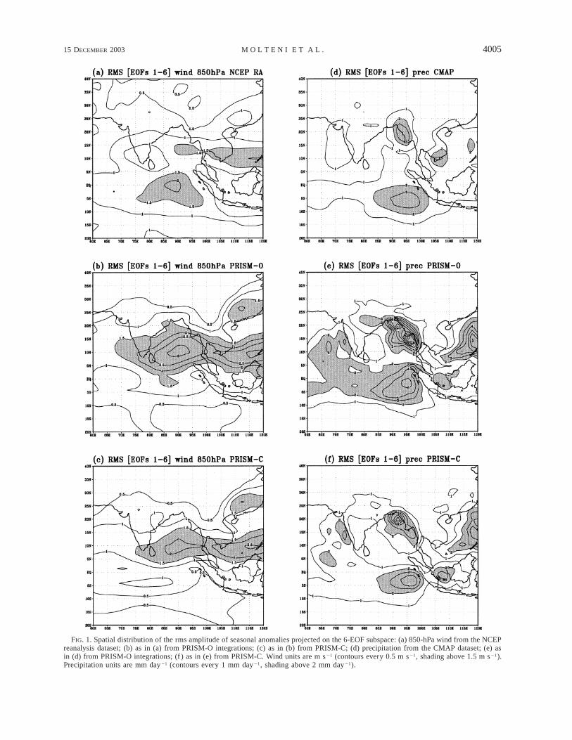
Figure 1 shows the spatial distribution of the rmsamplitude of seasonal-mean anomalies projected on the6-EOF subspace, for observational and model datasets.Contrary to spatially averaged values (Table 2), a bettercorrespondence between the modeled and observed dis-tribution of variability is found for rainfall than for 850-hPa wind. The three areas of large rainfall variabilityon the windward side of the Western Ghats, on the north-eastern margin of the Bay of Bengal, and just south ofthe equator in the eastern Indian Ocean are fairly wellreproduced by the model (although with a much strongeramplitude in the Bay of Bengal). Conversely, while thewind variability in the NCEP reanalysis shows a ratheruniform distribution between 208N and 108S, the modelvariability shows a marked concentration around 108N.Figure 1 also shows that the patterns of variability forPRISM-C are very similar to those of PRISM-O, sug-

gesting that interannual SST forcing only amplifies analready existing pattern of variability. This point willbe explored in greater depth in the next section.

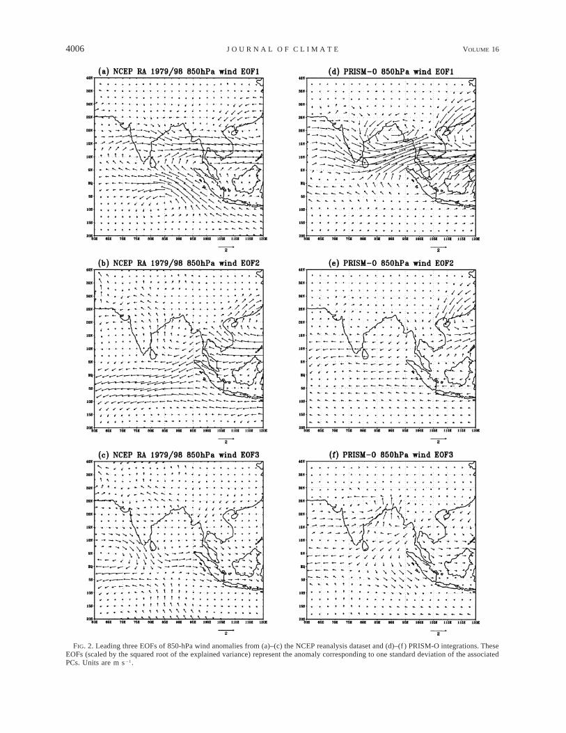
The reason for the discrepancy between the observedand simulated wind variability is easily understood bycomparing the patterns of the three leading EOFs of850-hPa wind from NCEP reanalysis and PRISM-O ex-periments, shown in Fig. 2. The first two wind EOFsfrom NCEP data in the 1979–98 period, shown in Figs.2a,b, are very similar (apart from arbitrary changes ofsign) to the two leading patterns found by Annamalaiet al. (1999) for the 1979–94 period. They explain asimilar proportion of variance, 26.9% and 22.1%, re-spectively. (Note that the EOFs plotted in the figuresare scaled by the square root of the explained variance,so that they represent the anomaly associated with onestandard deviation of the associated PC.)

The first EOF of the observations (Fig. 2a) explains26.9% of the total variance and is very similar to thefirst EOF of daily 850-hPa wind in the same domain,found by Sperber et al. (2000) from the full 40-yr recordof NCEP reanalysis. It shows a westerly anomaly span-ning the whole domain around 158N, with an easterlyanomaly over the Indian Ocean around the equator andtwo centers of cyclonic circulation in the northern partof the Bay of Bengal and over the South China Sea.The ECMWF model reproduces most of these featuresin the first EOF of PRISM-O (Fig. 2d), but with a gen-erally larger amplitude. It also explains a remarkable51.9% of the variance in PRISM-O data. However, theaxis of the strong westerly anomaly is shifted southward,around 108N, while the intensity of the easterly flowanomaly just south of the equator is underestimated. Themodel also fails to capture the alongshore wind anom-alies off the coast of Sumatra. These have been impli-cated in the development of the Indian Ocean Dipoleor Zonal Mode (e.g., Saji et al. 1999) and suggest thatif the model was coupled to the ocean it may havedifficulty in reproducing the correct variability in theIndian Ocean.

The second EOF of model data explains a much lowerproportion of variance (7.6%) than the second NCEPpattern (22.1%), and bears little resemblance to it in itsspatial structure. Therefore, while in the observationstwo patterns of comparable amplitude are needed toexplain half of the variance in the seasonal-mean wind,


FIG. 1. Spatial distribution of the rms amplitude of seasonal anomalies projected on the 6-EOF subspace: (a) 850-hPa wind from the NCEPreanalysis dataset; (b) as in (a) from PRISM-O integrations; (c) as in (b) from PRISM-C; (d) precipitation from the CMAP dataset; (e) asin (d) from PRISM-O integrations; (f ) as in (e) from PRISM-C. Wind units are m s21 (contours every 0.5 m s21, shading above 1.5 m s21).Precipitation units are mm day21 (contours every 1 mm day21, shading above 2 mm day21).


FIG. 2. Leading three EOFs of 850-hPa wind anomalies from (a)–(c) the NCEP reanalysis dataset and (d)–(f ) PRISM-O integrations. TheseEOFs (scaled by the squared root of the explained variance) represent the anomaly corresponding to one standard deviation of the associatedPCs. Units are m s21.


in the model the wind variability is dominated by justone pattern. A similar result was obtained by Ferrantiet al. (1997) using an earlier version of the ECMWFmodel. On the other hand, a relatively good agreementcan be found in the third EOF of observed and modeldata. This pattern, characterized by an anticyclonic cen-ter southwest of India and a cyclonic center over thenorthern part of the Indian subcontinent, resembles thewind pattern associated with positive anomalies of all-India rainfall found by Sperber et al. (2000). The cy-clonic flow over India is stronger in the model than inthe reanalysis, but overall the NCEP and PRISM-O pat-terns have comparable amplitudes and explained vari-ances (9.2% and 6.9%, respectively).

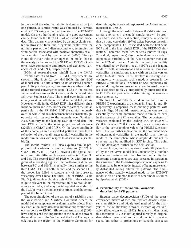
EOFs of seasonal-mean rainfall from the CMAP1979–98 dataset and from PRISM-O experiments areshown in Fig. 3. As for the wind EOFs, the first EOFof model data is quite similar to its observed counter-part. In its positive phase, it represents a northward shiftof the tropical convergence zone (TCZ) in the easternIndian and western Pacific Oceans, with increased rain-fall over Southeast Asia. The signal over India is rel-atively weak in both the observed and modeled pattern.However, while in the CMAP EOF it has different signsin the southern and in the northeastern parts of the Indianpeninsula, in the PRISM-O EOF the rainfall anomalyover the whole Indian subcontinent has a consistent sign,opposite with respect to the anomaly over SoutheastAsia. Contrary to the leading EOF of wind data, thefirst EOF explains the same proportion of variance(32.5%) in CMAP and PRISM-O; the larger amplitudeof the anomalies in the modeled pattern is therefore areflection of the overall larger rainfall variability in themodel simulations with respect to observations (see Ta-ble 2).

The second rainfall EOF also explains similar pro-portions of variance in the two datasets (13.2% inCMAP, 10.0% in PRISM-O); however, the spatial pat-terns are quite different from each other (cf. Figs. 3band 3e). The second EOF of PRISM-O, with three re-gions of alternating signs in the north–south directionbetween 808 and 1008E, is actually more similar to thethird CMAP EOF. In both the first and the second EOF,the model has failed to capture any of the observedvariability over China. The third EOF of PRISM-O (inFig. 3f), although explaining only 6.9% of the variance,is quite relevant to the representation of rainfall anom-alies over India, and may be interpreted as a shift ofthe TCZ between the Indian subcontinent and the centralpart of the Indian Ocean.

The poor simulation of the pattern of variability overthe west Pacific and Maritime Continent, where themodel behavior appears to be dominated by a local Had-ley circulation, may also have implications for the mod-el’s response to ENSO. Slingo and Annamalai (2000)have emphasized the importance of the balance betweenthe modulation of the Walker and the local Hadley cir-culations in the region of the Maritime Continent for

determining the observed response of the Asian summermonsoon to ENSO.

Although the relationship between 850-hPa wind andrainfall anomalies in the model simulations will be prop-erly addressed in the next section, it may be anticipatedthat a strong correlation (97%) exists between the prin-cipal components (PCs) associated with the first windEOF and to the first rainfall EOF of the PRISM-O sim-ulation. Therefore, these two patterns (shown in Figs.2d and 3d, respectively) describe the dominant mode ofinterannual variability of the Asian summer monsoonin the ECMWF model. A similar pattern of variabilitywas identified by Ferranti et al. (1997) as the leadingmode of both intraseasonal and interannual monsoonvariability in simulations made with an earlier versionof the ECMWF model. It is therefore interesting to in-vestigate to what extent such a mode is present in thePRISM-C simulations, in which no SST anomalies arepresent during the summer months, and internal dynam-ics is expected to play a proportionally larger role thanin PRISM-O experiments in determining the seasonal-mean anomalies.

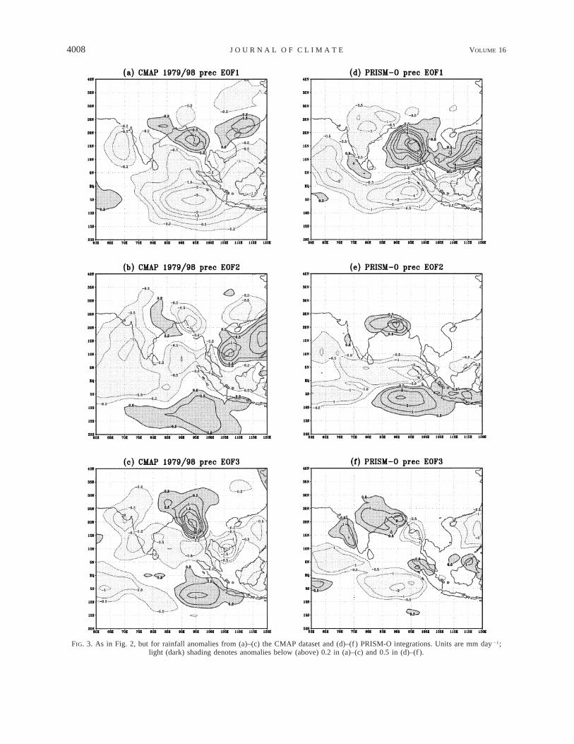
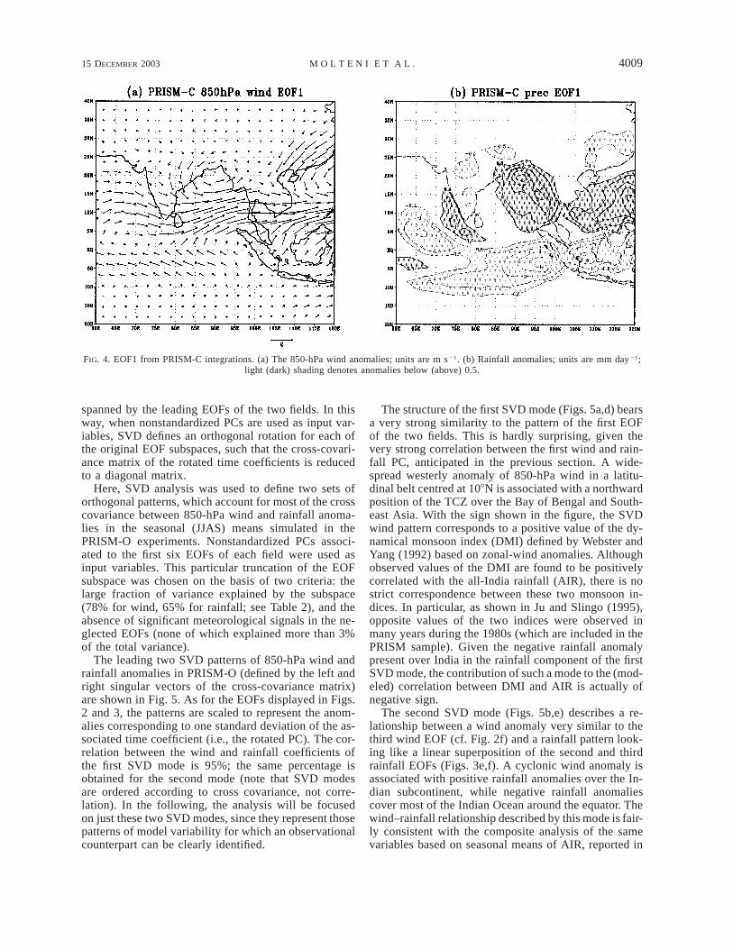
The first EOF of 850-hPa wind and rainfall from thePRISM-C experiments are shown in Figs. 4a and 4b,respectively. Comparing these anomaly patterns withthose in Figs. 2d and 3d, respectively, one can see thatessentially the same dominant mode is simulated evenin the absence of SST anomalies. The percentages ofvariance explained by the leading EOF in PRISM-C(53.0% for wind, 28.8% for rainfall) are also very sim-ilar to the corresponding values for PRISM-O ensem-bles. This is a further indication that the dominant modeof interannual variability in the model is an internalmode of the atmosphere whose amplitude but not itsstructure may be modified by SST forcing. This pointwill be developed further in the next section.

In conclusion, the seasonal-mean variability simulat-ed by the ECMWF model has undoubtedly a numberof common features with the observed variability, butimportant discrepancies are also present. In particular,the variance of the lower-tropospheric winds appears tobe dominated by one mode, instead of being more even-ly distributed among alternative patterns. The domi-nance of this zonally oriented mode in the ECMWFmodel is also a common feature of other models studiedby Sperber et al. (2001).

4. Predictability of interannual variationsdescribed by SVD patterns

Singular value decomposition (SVD) of the cross-covariance matrix of two multivariate datasets repre-sents an efficient and widely used method for the anal-ysis of the relationship between meteorological vari-ables (Bretherton et al. 1992). In many studies usingthis technique, SVD is not applied directly to originaldata defined over stations or grid points in physicalspace, but rather to projections on suitable subspaces


FIG. 3. As in Fig. 2, but for rainfall anomalies from (a)–(c) the CMAP dataset and (d)–(f ) PRISM-O integrations. Units are mm day 21;light (dark) shading denotes anomalies below (above) 0.2 in (a)–(c) and 0.5 in (d)–(f ).


FIG. 4. EOF1 from PRISM-C integrations. (a) The 850-hPa wind anomalies; units are m s21. (b) Rainfall anomalies; units are mm day21;light (dark) shading denotes anomalies below (above) 0.5.

spanned by the leading EOFs of the two fields. In thisway, when nonstandardized PCs are used as input var-iables, SVD defines an orthogonal rotation for each ofthe original EOF subspaces, such that the cross-covari-ance matrix of the rotated time coefficients is reducedto a diagonal matrix.

Here, SVD analysis was used to define two sets oforthogonal patterns, which account for most of the crosscovariance between 850-hPa wind and rainfall anoma-lies in the seasonal (JJAS) means simulated in thePRISM-O experiments. Nonstandardized PCs associ-ated to the first six EOFs of each field were used asinput variables. This particular truncation of the EOFsubspace was chosen on the basis of two criteria: thelarge fraction of variance explained by the subspace(78% for wind, 65% for rainfall; see Table 2), and theabsence of significant meteorological signals in the ne-glected EOFs (none of which explained more than 3%of the total variance).

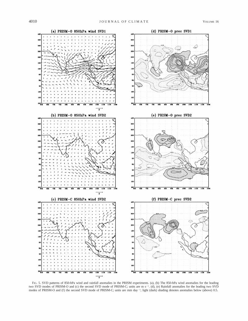
The leading two SVD patterns of 850-hPa wind andrainfall anomalies in PRISM-O (defined by the left andright singular vectors of the cross-covariance matrix)are shown in Fig. 5. As for the EOFs displayed in Figs.2 and 3, the patterns are scaled to represent the anom-alies corresponding to one standard deviation of the as-sociated time coefficient (i.e., the rotated PC). The cor-relation between the wind and rainfall coefficients ofthe first SVD mode is 95%; the same percentage isobtained for the second mode (note that SVD modesare ordered according to cross covariance, not corre-lation). In the following, the analysis will be focusedon just these two SVD modes, since they represent thosepatterns of model variability for which an observationalcounterpart can be clearly identified.

The structure of the first SVD mode (Figs. 5a,d) bearsa very strong similarity to the pattern of the first EOFof the two fields. This is hardly surprising, given thevery strong correlation between the first wind and rain-fall PC, anticipated in the previous section. A wide-spread westerly anomaly of 850-hPa wind in a latitu-dinal belt centred at 108N is associated with a northwardposition of the TCZ over the Bay of Bengal and South-east Asia. With the sign shown in the figure, the SVDwind pattern corresponds to a positive value of the dy-namical monsoon index (DMI) defined by Webster andYang (1992) based on zonal-wind anomalies. Althoughobserved values of the DMI are found to be positivelycorrelated with the all-India rainfall (AIR), there is nostrict correspondence between these two monsoon in-dices. In particular, as shown in Ju and Slingo (1995),opposite values of the two indices were observed inmany years during the 1980s (which are included in thePRISM sample). Given the negative rainfall anomalypresent over India in the rainfall component of the firstSVD mode, the contribution of such a mode to the (mod-eled) correlation between DMI and AIR is actually ofnegative sign.

The second SVD mode (Figs. 5b,e) describes a re-lationship between a wind anomaly very similar to thethird wind EOF (cf. Fig. 2f) and a rainfall pattern look-ing like a linear superposition of the second and thirdrainfall EOFs (Figs. 3e,f). A cyclonic wind anomaly isassociated with positive rainfall anomalies over the In-dian subcontinent, while negative rainfall anomaliescover most of the Indian Ocean around the equator. Thewind–rainfall relationship described by this mode is fair-ly consistent with the composite analysis of the samevariables based on seasonal means of AIR, reported in


FIG. 5. SVD patterns of 850-hPa wind and rainfall anomalies in the PRISM experiments. (a), (b) The 850-hPa wind anomalies for the leadingtwo SVD modes of PRISM-O and (c) the second SVD mode of PRISM-C; units are m s21. (d), (e) Rainfall anomalies for the leading two SVDmodes of PRISM-O and (f) the second SVD mode of PRISM-C; units are mm day21; light (dark) shading denotes anomalies below (above) 0.5.


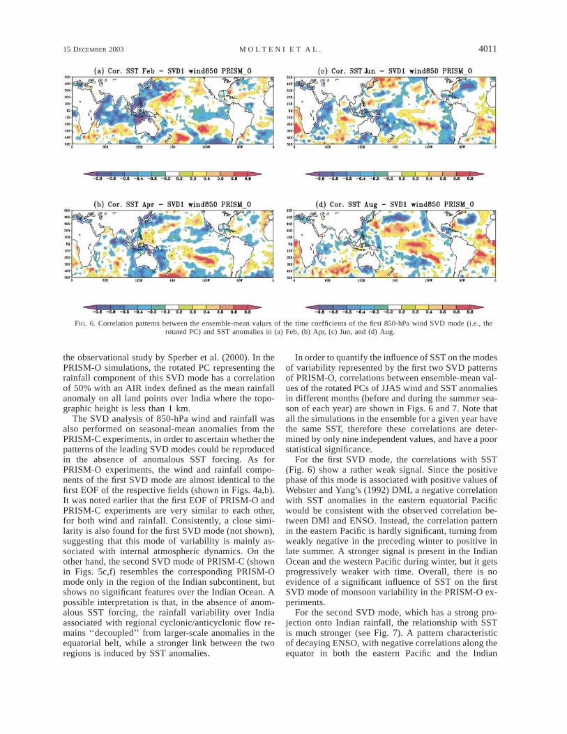
FIG. 6. Correlation patterns between the ensemble-mean values of the time coefficients of the first 850-hPa wind SVD mode (i.e., therotated PC) and SST anomalies in (a) Feb, (b) Apr, (c) Jun, and (d) Aug.

the observational study by Sperber et al. (2000). In thePRISM-O simulations, the rotated PC representing therainfall component of this SVD mode has a correlationof 50% with an AIR index defined as the mean rainfallanomaly on all land points over India where the topo-graphic height is less than 1 km.

The SVD analysis of 850-hPa wind and rainfall wasalso performed on seasonal-mean anomalies from thePRISM-C experiments, in order to ascertain whether thepatterns of the leading SVD modes could be reproducedin the absence of anomalous SST forcing. As forPRISM-O experiments, the wind and rainfall compo-nents of the first SVD mode are almost identical to thefirst EOF of the respective fields (shown in Figs. 4a,b).It was noted earlier that the first EOF of PRISM-O andPRISM-C experiments are very similar to each other,for both wind and rainfall. Consistently, a close simi-larity is also found for the first SVD mode (not shown),suggesting that this mode of variability is mainly as-sociated with internal atmospheric dynamics. On theother hand, the second SVD mode of PRISM-C (shownin Figs. 5c,f) resembles the corresponding PRISM-Omode only in the region of the Indian subcontinent, butshows no significant features over the Indian Ocean. Apossible interpretation is that, in the absence of anom-alous SST forcing, the rainfall variability over Indiaassociated with regional cyclonic/anticyclonic flow re-mains ‘‘decoupled’’ from larger-scale anomalies in theequatorial belt, while a stronger link between the tworegions is induced by SST anomalies.

In order to quantify the influence of SST on the modesof variability represented by the first two SVD patternsof PRISM-O, correlations between ensemble-mean val-ues of the rotated PCs of JJAS wind and SST anomaliesin different months (before and during the summer sea-son of each year) are shown in Figs. 6 and 7. Note thatall the simulations in the ensemble for a given year havethe same SST, therefore these correlations are deter-mined by only nine independent values, and have a poorstatistical significance.

For the first SVD mode, the correlations with SST(Fig. 6) show a rather weak signal. Since the positivephase of this mode is associated with positive values ofWebster and Yang’s (1992) DMI, a negative correlationwith SST anomalies in the eastern equatorial Pacificwould be consistent with the observed correlation be-tween DMI and ENSO. Instead, the correlation patternin the eastern Pacific is hardly significant, turning fromweakly negative in the preceding winter to positive inlate summer. A stronger signal is present in the IndianOcean and the western Pacific during winter, but it getsprogressively weaker with time. Overall, there is noevidence of a significant influence of SST on the firstSVD mode of monsoon variability in the PRISM-O ex-periments.

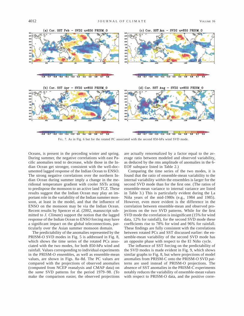
For the second SVD mode, which has a strong pro-jection onto Indian rainfall, the relationship with SSTis much stronger (see Fig. 7). A pattern characteristicof decaying ENSO, with negative correlations along theequator in both the eastern Pacific and the Indian


FIG. 7. As in Fig. 6 but for the rotated PC associated with the second 850-hPa wind SVD mode.

Oceans, is present in the preceding winter and spring.During summer, the negative correlations with east Pa-cific anomalies tend to decrease, while those in the In-dian Ocean get stronger, consistent with the well-doc-umented lagged response of the Indian Ocean to ENSO.The strong negative correlations over the northern In-dian Ocean during summer imply a change in the me-ridional temperature gradient with cooler SSTs actingto predispose the monsoon to an active land TCZ. Theseresults suggest that the Indian Ocean may play an im-portant role in the variability of the Indian summer mon-soon, at least in the model, and that the influence ofENSO on the monsoon may be via the Indian Ocean.Recent results by Spencer et al. (2002, manuscript sub-mitted to J. Climate) support the notion that the laggedresponse of the Indian Ocean to ENSO forcing may havea significant impact on the global teleconnections, par-ticularly over the Asian summer monsoon domain.

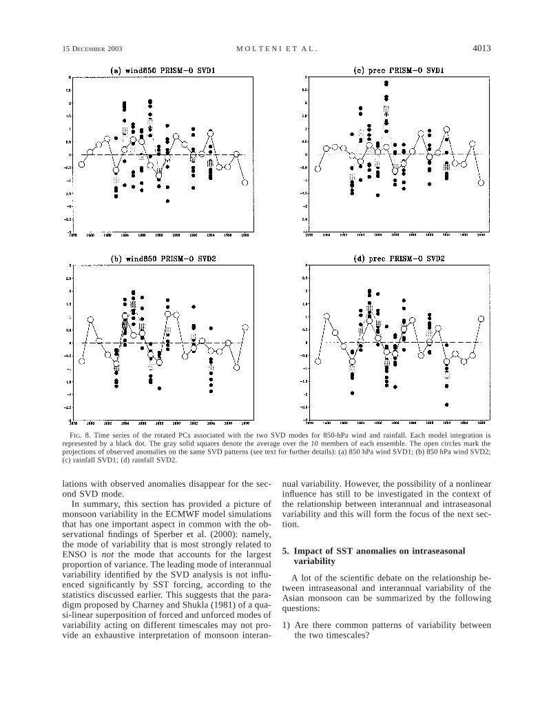
The predictability of the anomalies represented by thePRISM-O SVD modes in Fig. 5 is addressed in Fig. 8,which shows the time series of the rotated PCs asso-ciated with the two modes, for both 850-hPa wind andrainfall. Values corresponding to individual experimentsin the PRISM-O ensembles, as well as ensemble-meanvalues, are shown in Figs. 8a–8d. The PC values arecompared with the projections of observed anomalies(computed from NCEP reanalysis and CMAP data) onthe same SVD patterns for the period 1979–98. (Tomake the comparison easier, the observed projections

are actually renormalized by a factor equal to the av-erage ratio between modeled and observed variability,as deduced by the rms amplitude of anomalies in the 6-EOF subspace listed in Table 2.)

Comparing the time series of the two modes, it isfound that the ratio of ensemble-mean variability to theinternal variability within the ensembles is larger for thesecond SVD mode than for the first one. (The ratios ofensemble-mean variance to internal variance are listedin Table 3.) This is particularly evident during the LaNina years of the mid-1980s (e.g., 1984 and 1985).However, even more evident is the difference in thecorrelation between ensemble-mean and observed pro-jections on the two SVD patterns. While for the firstSVD mode the correlation is insignificant (15% for winddata, 12% for rainfall), for the second SVD mode thesecoefficients rise to 78% for wind and 96% for rainfall.These findings are fully consistent with the correlationsbetween rotated PCs and SST discussed earlier: the en-semble-mean variability of the second SVD mode hasan opposite phase with respect to the El Nino cycle.

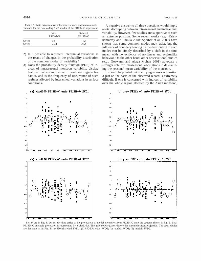
The influence of SST forcing on the predictability ofthe SVD modes is made evident in Fig. 9, which showssimilar graphs to Fig. 8, but where projections of modelanomalies from PRISM-C onto the PRISM-O SVD pat-terns are used instead of PRISM-O projections. Theabsence of SST anomalies in the PRISM-C experimentsnotably reduces the variability of ensemble-mean valueswith respect to PRISM-O data, and the positive corre-


FIG. 8. Time series of the rotated PCs associated with the two SVD modes for 850-hPa wind and rainfall. Each model integration isrepresented by a black dot. The gray solid squares denote the average over the 10 members of each ensemble. The open circles mark theprojections of observed anomalies on the same SVD patterns (see text for further details): (a) 850 hPa wind SVD1; (b) 850 hPa wind SVD2;(c) rainfall SVD1; (d) rainfall SVD2.

lations with observed anomalies disappear for the sec-ond SVD mode.

In summary, this section has provided a picture ofmonsoon variability in the ECMWF model simulationsthat has one important aspect in common with the ob-servational findings of Sperber et al. (2000): namely,the mode of variability that is most strongly related toENSO is not the mode that accounts for the largestproportion of variance. The leading mode of interannualvariability identified by the SVD analysis is not influ-enced significantly by SST forcing, according to thestatistics discussed earlier. This suggests that the para-digm proposed by Charney and Shukla (1981) of a qua-si-linear superposition of forced and unforced modes ofvariability acting on different timescales may not pro-vide an exhaustive interpretation of monsoon interan-

nual variability. However, the possibility of a nonlinearinfluence has still to be investigated in the context ofthe relationship between interannual and intraseasonalvariability and this will form the focus of the next sec-tion.

5. Impact of SST anomalies on intraseasonalvariability

A lot of the scientific debate on the relationship be-tween intraseasonal and interannual variability of theAsian monsoon can be summarized by the followingquestions:

1) Are there common patterns of variability betweenthe two timescales?


TABLE 3. Ratio between ensemble-mean variance and intraensemblevariance for the two leading SVD modes of the PRISM-O experiment.

WindPRISM-O

RainfallPRISM-O

SVD1SVD2

0.812.78

1.532.54

FIG. 9. As in Fig. 8, but for the time series of the projections of model anomalies from PRISM-C onto the patterns shown in Fig. 5. EachPRISM-C anomaly projection is represented by a black dot. The gray solid squares denote the ensemble-mean projection. The open circlesare the same as in Fig. 8: (a) 850-hPa wind SVD1; (b) 850-hPa wind SVD2; (c) rainfall SVD1; (d) rainfall SVD2.

2) Is it possible to represent interannual variations asthe result of changes in the probability distributionof the common modes of variability?

3) Does the probability density function (PDF) of in-dices of intraseasonal monsoon variability displayfeatures that are indicative of nonlinear regime be-havior, and is the frequency of occurrence of suchregimes affected by interannual variations in surfaceconditions?

A negative answer to all three questions would implya total decoupling between intraseasonal and interannualvariability. However, few studies are supportive of suchan extreme position. Some recent works (e.g., Krish-namurthy and Shukla 2000; Sperber et al. 2000) haveshown that some common modes may exist, but theinfluence of boundary forcing on the distribution of suchmodes can be simply described by a shift in the timemean, with no evidence of nonlinear and regimelikebehavior. On the other hand, other observational studies(e.g., Goswami and Ajaya Mohan 2001) advocate astronger role for intraseasonal oscillations in determin-ing the seasonal-mean variability of the monsoon.

It should be pointed out that trying to answer question3 just on the basis of the observed record is extremelydifficult. If one is concerned with indices of variabilityover the whole region affected by the Asian monsoon,


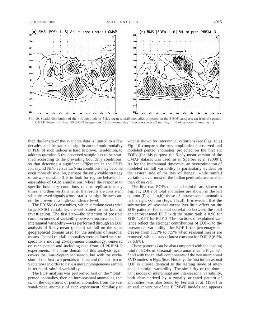
FIG. 10. Spatial distribution of the rms amplitude of 5-day-mean rainfall anomalies projected on the 6-EOF subspace: (a) from the pentadCMAP dataset; (b) from PRISM-O integrations. Units are mm day21 (contours every 2 mm day21, shading above 6 mm day21).

then the length of the available data is limited to a fewdecades, and the statistical significance of multimodalityin PDF of such indices is hard to prove. In addition, toaddress question 3 the observed sample has to be strat-ified according to the prevailing boundary conditions,so that detecting a significant difference in the PDFsfor, say, El Nino versus La Nina conditions may becomeeven more elusive. So, perhaps the only viable strategyto answer question 3 is to look for regime behavior inensembles of GCM simulations, where the response tospecific boundary conditions can be replicated manytimes, and then verify whether the results are consistentwith observed signals whose statistical significance can-not be proven at a high-confidence level.

The PRISM-O ensembles, which simulate years withlarge ENSO variability, are well suited to this kind ofinvestigation. The first step—the detection of possiblecommon modes of variability between intraseasonal andinterannual variability—was performed through an EOFanalysis of 5-day-mean (pentad) rainfall on the samegeographical domain used for the analysis of seasonalmeans. Pentad rainfall anomalies were defined with re-spect to a moving 25-day-mean climatology, centeredon each pentad and including data from all PRISM-Oexperiments. The time domain of this analysis againcovers the June–September season, but with the exclu-sion of the first two pentads of June and the last two ofSeptember in order to have a more homogeneous samplein terms of rainfall variability.

The EOF analysis was performed first on the ‘‘total’’pentad anomalies, then on intraseasonal anomalies, thatis, on the departures of pentad anomalies from the sea-sonal-mean anomaly of each experiment. Similarly to

what is shown for interannual variations (see Figs. 1d,e)Fig. 10 compares the rms amplitude of observed andmodeled pentad anomalies projected on the first sixEOFs [for this purpose the 5-day-mean version of theCMAP dataset was used, as in Sperber et al. (2000)].As for the interannual timescale, an overestimation ofmodeled rainfall variability is particularly evident onthe eastern side of the Bay of Bengal, while rainfallvariations over most of the Indian peninsula are smallerthan observed.

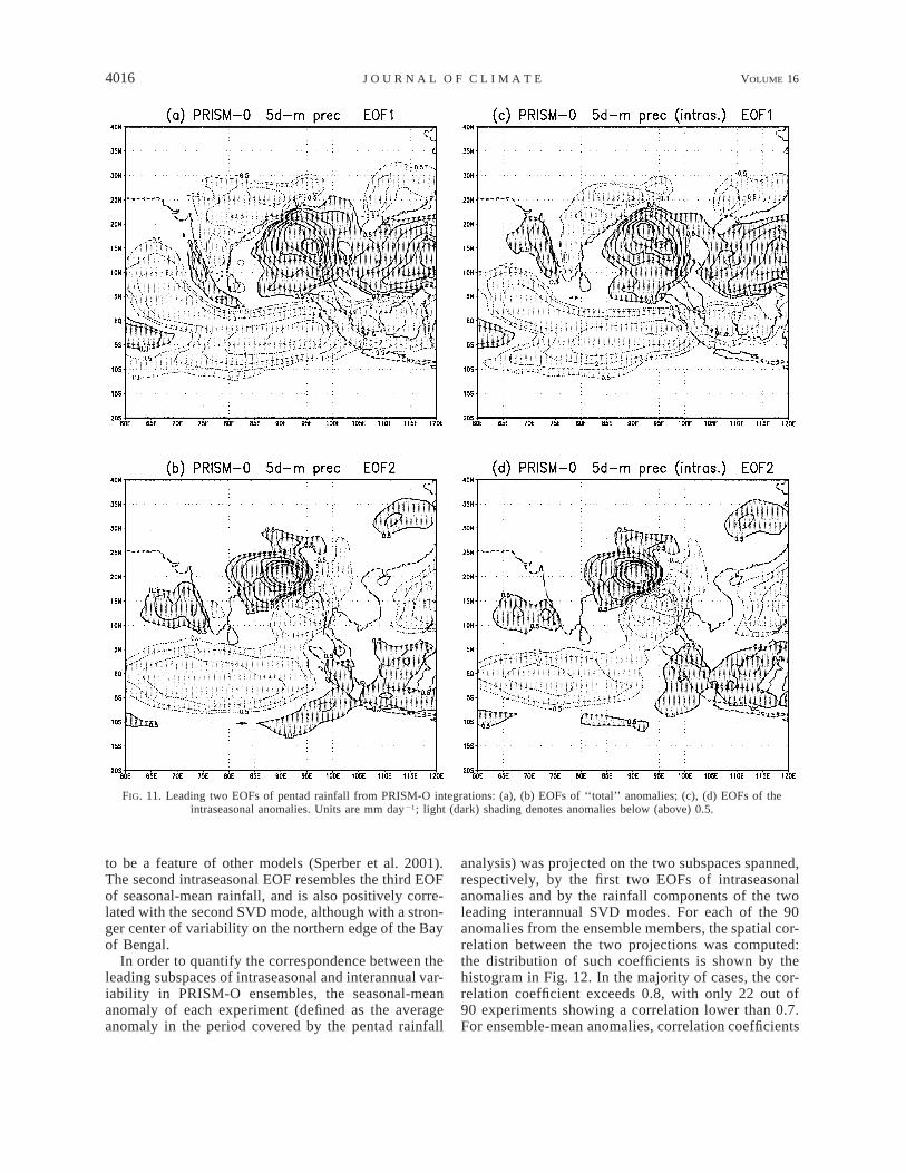
The first two EOFs of pentad rainfall are shown inFig. 11; EOFs of total anomalies are shown in the leftcolumn (Figs. 11a,b), those of intraseasonal anomaliesin the right column (Figs. 11c,d). It is evident that thesubtraction of seasonal means has little effect on theEOF patterns: the spatial correlation between the totaland intraseasonal EOF with the same rank is 0.96 forEOF-1, 0.97 for EOF-2. The fractions of explained var-iance reflect the stronger contributions of EOF-1 to theinterannual variability—for EOF-1, the percentage de-creases from 11.1% to 7.5% when seasonal means areremoved, while it stays almost constant for EOF-2 (6.5%vs 6.6%).

These patterns can be also compared with the leadingrainfall EOFs of seasonal-mean anomalies in Figs. 3d–f and with the rainfall components of the two interannualSVD modes in Figs. 5d,e. Notably, the first intraseasonalEOF is almost identical to the leading mode of inter-annual rainfall variability. The similarity of the domi-nant modes of interannual and intraseasonal variability,both characterized by a zonally oriented pattern ofanomalies, was also found by Ferranti et al. (1997) inan earlier version of the ECMWF models and appears


FIG. 11. Leading two EOFs of pentad rainfall from PRISM-O integrations: (a), (b) EOFs of ‘‘total’’ anomalies; (c), (d) EOFs of theintraseasonal anomalies. Units are mm day21; light (dark) shading denotes anomalies below (above) 0.5.

to be a feature of other models (Sperber et al. 2001).The second intraseasonal EOF resembles the third EOFof seasonal-mean rainfall, and is also positively corre-lated with the second SVD mode, although with a stron-ger center of variability on the northern edge of the Bayof Bengal.

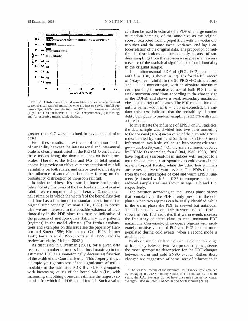
In order to quantify the correspondence between theleading subspaces of intraseasonal and interannual var-iability in PRISM-O ensembles, the seasonal-meananomaly of each experiment (defined as the averageanomaly in the period covered by the pentad rainfall

analysis) was projected on the two subspaces spanned,respectively, by the first two EOFs of intraseasonalanomalies and by the rainfall components of the twoleading interannual SVD modes. For each of the 90anomalies from the ensemble members, the spatial cor-relation between the two projections was computed:the distribution of such coefficients is shown by thehistogram in Fig. 12. In the majority of cases, the cor-relation coefficient exceeds 0.8, with only 22 out of90 experiments showing a correlation lower than 0.7.For ensemble-mean anomalies, correlation coefficients


FIG. 12. Distribution of spatial correlations between projections ofseasonal-mean rainfall anomalies onto the first two SVD rainfall pat-terns (Figs. 5d–5e) and the first two EOFs of intraseasonal rainfall(Figs. 11c–11d), for individual PRISM-O experiments (light shading)and for ensemble means (dark shading).

greater than 0.7 were obtained in seven out of ninecases.

From these results, the existence of common modesof variability between the intraseasonal and interannualscale is clearly manifested in the PRISM-O ensembles,these modes being the dominant ones on both time-scales. Therefore, the EOFs and PCs of total pentadanomalies provide an effective representation of rainfallvariability on both scales, and can be used to investigatethe influence of anomalous boundary forcing on theprobability distribution of monsoon rainfall.

In order to address this issue, bidimensional proba-bility density functions of the two leading PCs of pentadrainfall were computed using an iterative Gaussian ker-nel estimator in which the width h of the kernel functionis defined as a fraction of the standard deviation of theoriginal time series (Silverman 1981, 1986). In partic-ular, we are interested in the possible existence of mul-timodality in the PDF, since this may be indicative ofthe presence of multiple quasi-stationary flow patterns(regimes) in the model climate. (For further explana-tions and examples on this issue see the papers by Han-sen and Sutera 1986; Kimoto and Ghil 1993; Palmer1994; Ferranti et al. 1997; Corti et al. 1999; and thereview article by Molteni 2003.)

As discussed in Silverman (1981), for a given datarecord, the number of modes (i.e., local maxima) in theestimated PDF is a monotonically decreasing functionof the width of the Gaussian kernel. This property allowsa simple yet rigorous test of the significance of multi-modality in the estimated PDF. If a PDF is computedwith increasing values of the kernel width (i.e., withincreasing smoothing), one can estimate the largest val-ue of h for which the PDF is multimodal. Such a value

can then be used to estimate the PDF of a large numberof random samples, of the same size as the originalrecord, extracted from a population with unimodal dis-tribution and the same mean, variance, and lag-1 au-tocorrelation of the original data. The proportion of mul-timodal distributions obtained (simply because of ran-dom sampling) from the red-noise samples is an inversemeasure of the statistical significance of multimodalityin the original sample.

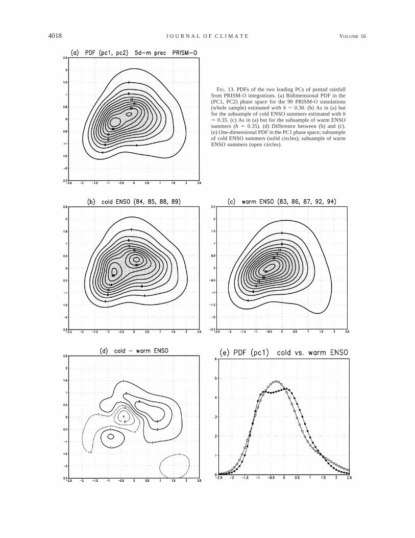
The bidimensional PDF of (PC1, PC2), estimatedwith h 5 0.30, is shown in Fig. 13a for the full recordof 5-day-mean rainfall in the 90 PRISM-O simulations.The PDF is nonisotropic, with an absolute maximumcorresponding to negative values of both PCs (i.e., ofweak monsoon conditions according to the chosen signof the EOFs), and shows a weak secondary maximumclose to the origin of the axes. The PDF remains bimodaluntil a kernel width of h 5 0.35 is exceeded; the ran-dom-noise test indicates that the probability of bimo-dality being due to random sampling is 12.2% with sucha threshold.

To investigate the influence of ENSO on PC statistics,the data sample was divided into two parts accordingto the seasonal (JJAS) mean value of the bivariate ENSOindex defined by Smith and Sardeshmukh (2000; moreinformation available online at http://www.cdc.noaa.gov/;cas/best/#years).1 Of the nine summers coveredby PRISM-O ensembles, four (1984, 1985, 1988, 1989)have negative seasonal-mean indices with respect to amultidecadal mean, corresponding to cold events in theeastern tropical Pacific, while the other five summersare representative of warm events. The PDFs obtainedfrom the two subsamples of cold and warm ENSO sum-mers (estimated with h 5 0.35 to compensate for thereduced sample size) are shown in Figs. 13b and 13c,respectively.

The partition according to the ENSO phase showsthat bimodality in the PDF is only present in the coldphase, when two regimes can be easily identified, whilein the warm phase the PDF is skewed but unimodal.The difference between PDFs in warm and cold ENSO,shown in Fig. 13d, indicates that warm events increasethe frequency of states close to weak-monsoon PDFmaximum. Conversely, phase-space regions with mod-erately positive values of PC1 and PC2 become morepopulated during cold events, when a second mode isestablished.

Neither a simple shift in the mean state, nor a changeof frequency between two ever-present regimes, seemsthe most appropriate description for the PDF changesbetween warm and cold ENSO events. Rather, thesechanges are suggestive of some sort of bifurcation in

1 The seasonal means of the bivariate ENSO index were obtainedby averaging the JJAS monthly values of the time series. In someyears, the JJAS averages do not have the same sign as the winteraverages listed in Table 1 of Smith and Sardeshmukh (2000).


FIG. 13. PDFs of the two leading PCs of pentad rainfallfrom PRISM-O integrations. (a) Bidimensional PDF in the(PC1, PC2) phase space for the 90 PRISM-O simulations(whole sample) estimated with h 5 0.30. (b) As in (a) butfor the subsample of cold ENSO summers estimated with h5 0.35. (c) As in (a) but for the subsample of warm ENSOsummers (h 5 0.35). (d) Difference between (b) and (c).(e) One-dimensional PDF in the PC1 phase space; subsampleof cold ENSO summers (solid circles); subsample of warmENSO summers (open circles).


the monsoon properties, with a multiple-regime behav-ior being established only when the zonal asymmetriesin equatorial Pacific SST exceed a threshold value. Mol-teni and Corti (1998) noted a similar behavior in qua-sigeostrophic simulations of North Pacific Ocean large-scale anomalies, again finding that a forcing pattern cor-responding to warm ENSO conditions induced unimo-dality in an otherwise bimodal PDF. The emergence ofbimodality in certain years was also noted in Ferrantiet al. (1997), but in their case only when the intrasea-sonal mode was particularly active.

In such a situation, it is perhaps more appropriate totest the significance of the bimodality in the cold ENSOPDF, rather than in the PDF of the full sample. Thesmaller size of the subsample (40 versus 90 simulations)is bound to reduce the confidence for the same value ofthe smoothing parameter. However, the cold ENSO PDFis still bimodal when estimated with h 5 0.40 (notshown), when only 8.6% of red-noise PDFs appear tobe multimodal.

Although it is better revealed by bidimensional es-timates, the transition from unimodal to bimodal dis-tribution in opposite ENSO phases is also detectable inone-dimensional PDF estimates for the first PC only,shown in Fig. 13e. In one dimension, multimodality canbe significantly detected for smaller values of h than in2D estimates, therefore a value of h 5 0.25 was usedhere. In this case, the chance of ‘‘spurious’’ bimodalityin the cold ENSO subsample, estimated from red-noisedata, is as low as 4.4%, with a level of significanceexceeding 95%.

It should be stressed that these model results do notguarantee the existence of regimes in the observed mon-soon circulation. As mentioned above, the detection ofregime behavior is rather difficult from observationalrecords, because of longer timescale changes in the forc-ing and because of the presence of interdecadal trendsin the monsoon circulation given in the NCEP reanal-yses. For example, Sperber et al. (2000) found that thedominant mode of interannual variability in the windsfrom the NCEP reanalyses represented the decadal time-scale weakening of the monsoon circulation associatedwith the warming of the Indian Ocean over the last 40yr. However, the PRISM-O results do show that regimebehavior is not only a feature of low-order dynamicalmodels, although a simple ‘‘extrapolation’’ of the be-havior of such models may be inappropriate. As a con-sequence, significance tests applied to observed datashould reflect the ‘‘dynamical plausibility’’ of the re-gime hypothesis, when compared with standard null hy-potheses derived from purely statistical reasoning.

6. Summary and conclusions

The effects of SST anomalies on the interannual andintraseasonal variability of the Asian summer monsoonhave been investigated by multivariate statistical anal-yses of 850-hPa wind and rainfall fields from a set of

ensemble simulations performed with the ECMWF at-mospheric GCM, referred to as the PRISM experiments.In particular, analyses have focused on simulations ofthe northern summer circulation over south Asia usingobserved SST (PRISM-O experiments), which covered9 yr characterized by large variations of the ENSO phe-nomenon in the 1980s and the early 1990s.

The main results of our analyses can be summarizedas follows:

• The dominant mode of interannual variability of theAsian summer monsoon, as simulated by the ECMWFmodel, consists of a zonally coherent anomaly of 850-hPa wind centered at 108N, associated with a merid-ional shift of the TCZ from the equatorial IndianOcean to the Bay of Bengal and Southeast Asia. Al-though a similar variability pattern is found in obser-vational data, the ECMWF model overestimates thefraction of variance explained by this mode, partic-ularly of its wind component.

• The second mode of variability emerging from theSVD analyses of wind and rainfall fields also has agood correspondence with observed patterns of var-iability. In its positive phase, a cyclonic wind anomalyis associated with positive rainfall anomalies over theIndian subcontinent, while negative rainfall anomaliesprevail over the Indian Ocean near the equator.

• While the association between the first SVD modeand SST anomalies is rather weak, leading to a poorpredictability of its interannual variability, the secondmode shows a clear relationship to the ENSO cycle.As a consequence, the interannual variations of theamplitude of SVD-2 anomalies are successfully sim-ulated by the ensemble means, with a correlation of96% between modeled and observed values of theassociated rainfall index.

• An EOF analysis of 5-day-mean rainfall from PRISM-O ensembles revealed a strong similarity between thedominant patterns of rainfall variability on the inter-annual and intraseasonal scale. Although seasonal-mean values of the PC associated with the leadingrainfall pattern shows no significant correlation withthe ENSO index, the two-dimensional probability dis-tribution of the leading 5-day-mean PC indices isturned from unimodal in the warm phase of ENSO tobimodal in the cold ENSO phase.

These findings contain a mixture of good and badnews as far as the prospects for numerical seasonal pre-dictions of the Asian monsoon are concerned. On theone hand, the high correlation coefficients between ob-served and simulated (ensemble mean) values of theSVD-2 index, which is related to the all-India rainfallindex, represent a notable and encouraging result. Onthe other hand, consistent with the observational studyof Sperber et al. (2000), the PRISM-O simulations in-dicate that the mode of monsoon variability most strong-ly related to ENSO is not the one that accounts for thelargest proportion of variance. Additionally, it should


be noted that our numerical simulations of monsoonvariability patterns were affected by significant dis-crepancies from observations in the partition of variancebetween modes with different regional characteristics.

With regard to a theoretical understanding of mon-soon dynamics, and particularly of the impact of bound-ary forcing on the statistics of intraseasonal variability,PRISM results highlight the limitations of the simpleparadigms proposed so far for the interpretation of sucha relationship. As stated earlier, neither a simple shiftin the mean state, nor a change of frequency betweentwo ever-present regimes, is an appropriate descriptionfor the PDF changes between warm and cold ENSOevents in PRISM-O simulations. The change in the PDFfrom unimodal to bimodal according to the ENSO phaseis rather suggestive of some type of bifurcation process,such as those encountered in the study of many nonlin-ear dynamical systems when forcing parameters arechanged in a continuous way.

On the basis of this study, we cannot state whetherthe PRISM-O results on this issue are confirmed byobservations. However, the detection of regimelike be-havior in the monsoon simulations by a complex nu-merical model gives a stronger appeal to this dynamicalframework than simple qualitative arguments based onthe analogy with low-order nonlinear systems.

Acknowledgments. The authors are grateful to ananonymous referee for his constructive suggestions. ThePRISM experiments were performed with computingtime provided through an ECMWF Special Project. JuliaSlingo acknowledges the support of the NERC UK Uni-versities’ Global Atmospheric Modelling Programme(UGAMP).

REFERENCES

Annamalai, H., J. M. Slingo, K. R. Sperber, and K. Hodges, 1999:The mean evolution and variability of the Asian summer mon-soon: Comparison of ECMWF and NCEP–NCAR reanalyses.Mon. Wea. Rev., 127, 1157–1186.

Bamzai, A. S., and L. Marx, 2000: COLA AGCM simulations of theeffect of anomalous spring snow cover over Eurasia on the Indiansummer monsoon. Quart. J. Roy. Meteor. Soc., 126, 2575–2584.

Becker, B. D., J. M. Slingo, L. Ferranti, and F. Molteni, 2001: Seasonalpredictability of the Indian summer monsoon: What role do land-surface conditions play? Mausam, 52, 175–190.

Blandford, H. F., 1884: On the connection of the Himalaya snowfallwith dry winds and seasons of drought in India. Proc. Roy. Soc.London, 37, 3–22.

Bretherton, C. S., C. Smith, and J. M. Wallace, 1992: An intercom-parison of methods for finding coupled patterns in climate data.J. Climate, 5, 541–560.

Charney, J. G., and J. Shukla, 1981: Predictability of monsoon. Mon-soon Dynamics, J. Lighthill and R. P. Pearce, Eds., CambridgeUniversity Press, 99–110.

Corti, S., F. Molteni, and T. N. Palmer, 1999: Signature of recentclimate change in frequencies of natural atmospheric circulationregimes. Nature, 398, 799–802.

——, ——, and ——, 2000: Predictability of snow-depth anomaliesover Eurasia and associated circulation patterns. Quart. J. Roy.Meteor. Soc., 126, 241–262.

Dong, B., and P. J. Valdes, 1998: Modelling the Asian summer mon-soon rainfall and Eurasian winter/spring snow mass. Quart. J.Roy. Meteor. Soc., 124, 2567–2596.

Douville, H., and J.-F. Royer, 1996: Sensitivity of the Asian summermonsoon to an anomalous Eurasian snow cover within the Me-teo-France GCM. Climate Dyn., 12, 449–466.

Ferranti, L., and F. Molteni, 1999: Ensemble simulations of Eurasiansnow-depth anomalies and their influence on the Asian summermonsoon. Quart. J. Roy. Meteor. Soc., 125, 2597–2610.

——, J. M. Slingo, T. N. Palmer, and B. J. Hoskins, 1997: Relationsbetween interannual and intraseasonal monsoon variability asdiagnosed from AMIP integrations. Quart. J. Roy. Meteor. Soc.,123, 1323–1357.

Gibson, J. K., P. Kallberg, S. Uppala, A. Hernandez, A. Nomura, andE. Serrano, 1997: ERA-15 description. ECMWF Re-AnalysisProject Rep. 1, 74 pp.

Goswami, B. N., and R. S. Ajaya Mohan, 2001: Intraseasonal oscil-lations and interannual variability of the Indian summer mon-soon. J. Climate, 14, 1180–1198.

Hansen, A. R., and A. Sutera, 1986: On the probability density dis-tribution of large-scale atmospheric wave amplitude. J. Atmos.Sci., 43, 3250–3265.

Ju, J., and J. M. Slingo, 1995: The Asian monsoon and ENSO. Quart.J. Roy. Meteor. Soc., 121, 1133–1168.

Kalnay, E., and Coauthors, 1996: The NCEP/NCAR 40-Year Re-analysis Project. Bull. Amer. Meteor. Soc., 77, 437–471.

Kang, I.-S., and Coauthors, 2002: Intercomparison of the climato-logical variations of Asian summer monsoon precipitation sim-ulated by 10 GCMs. Climate Dyn., 19, 383–395.

Kimoto, M., and M. Ghil, 1993: Multiple flow regimes in the NorthernHemisphere winter. Part I: Methodology and hemispheric re-gimes. J. Atmos. Sci., 50, 2625–2643.

Krishnamurthy, V., and J. Shukla, 2000: Intraseasonal and interannualvariability of rainfall over India. J. Climate, 13, 4366–4377.

Molteni, F., 2003: Weather regimes and multiple equilibria. Encyclo-pedia of Atmospheric Sciences, J. R. Holton et al., Eds., Aca-demic Press, 2577–2586.

——, and S. Corti, 1998: Long-term fluctuations of the statisticalproperties of low-frequency variability: Dynamical origin andpredictability. Quart. J. Roy. Meteor. Soc., 124, 495–526.

Palmer, T. N., 1994: Chaos and predictability in forecasting the mon-soon. Proc. Indian Natl. Sci. Acad., 60, 57–66.

Ritchie, H., C. Temperton, A. Simmons, M. Hortal, T. Davies, D.Dent, and M. Hamrud, 1995: Implementation of the semi-La-grangian method in a high-resolution version of the ECMWFforecast model. Mon. Wea. Rev., 123, 490–514.

Saji, N. H., B. N. Goswami, P. N. Vinayachandran, and T. Yamagata,1999: A dipole mode in the tropical Indian Ocean. Nature, 401,360–363.

Silverman, B. W., 1981: Using kernel-density estimators to investi-gate multimodality. J. Roy. Stat. Soc., 43B, 97–99.

——, 1986: Density Estimation for Statistics and Data Analysis.Chapman and Hall, 175 pp.

Slingo, J. M., and H. Annamalai, 2000: The El Nino of the centuryand the response of the Indian Summer Monsoon. Mon. Wea.Rev., 128, 1778–1797.

Smith, C. A., and P. Sardeshmukh, 2000: The effect of ENSO on theintraseasonal variance of surface temperature in winter. Int. J.Climatol., 20, 1543–1557.

Soman, M. K., and J. M. Slingo, 1997: Sensitivity of Asian summermonsoon to aspects of sea surface temperature anomalies in thetropical Pacific Ocean. Quart. J. Roy. Meteor. Soc., 123, 309–336.

Sperber, K. R., J. M. Slingo, and H. Annamalai, 2000: Predictabilityand the relationship between subseasonal and interannual vari-ability during the Asian summer monsoon. Quart. J. Roy. Me-teor. Soc., 126, 2545–2574.

——, and Coauthors, 2001: Dynamical seasonal predictability of theAsian summer monsoon. Mon. Wea. Rev., 129, 2226–2248.

von Storch, H., and F. W. Zwiers, 1999: Statistical Analysis in ClimateResearch. Cambridge University Press, 484 pp.


Webster, P. J., and S. Yang, 1992: Monsoon and ENSO: Selectivelyinteractive systems. Quart. J. Roy. Meteor. Soc., 118, 877–926.

——, V. O. Magana, T. N. Palmer, J. Shukla, R. A. Tomas, M. Yanai,and T. Yasunari, 1998: Monsoons: Processes, predictability, andprospects for prediction. J. Geophys. Res., 103, 14 451–14 510.

Wilks, D. S., 1995: Statistical Methods in the Atmospheric Sciences.Academic Press, 465 pp.

Xie, P., and P. Arkin, 1997: Global precipitation: A 17-year monthlyanalysis based on gauge observations, satellite estimates, and nu-merical model outputs. Bull. Amer. Meteor. Soc., 78, 2539–2558.

predictability experiments for the asian summer monsoon: impact of sst anomalies on interannual and...

Documents