towards gambit 2.0 - cern indico
TRANSCRIPT
Towards GAMBIT 2.0Anders Kvellestad, University of Osloon behalf of the GAMBIT CollaborationReinterpretation Forum 2021 — Feb 19, 2021
G AM B I T
Anders Kvellestad
Outline
2
1. Global fits
2. GAMBIT
3. GUM
G AM B I T
Anders Kvellestad 3
1. Global fits
G AM B I T
Anders Kvellestad 4
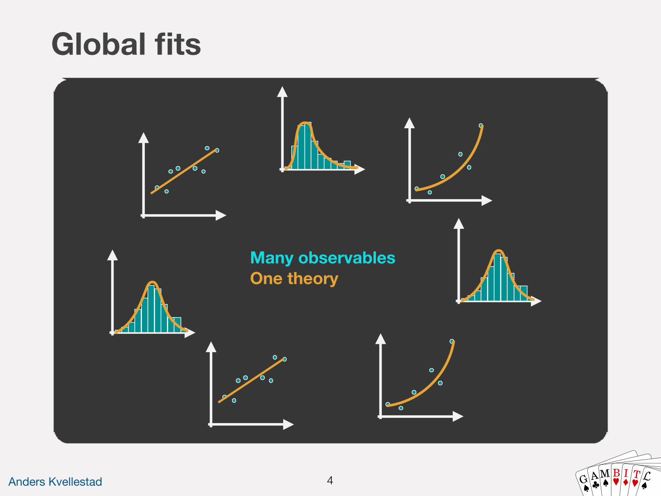
Global fits
Many observablesOne theory
G AM B I T
Anders Kvellestad 5
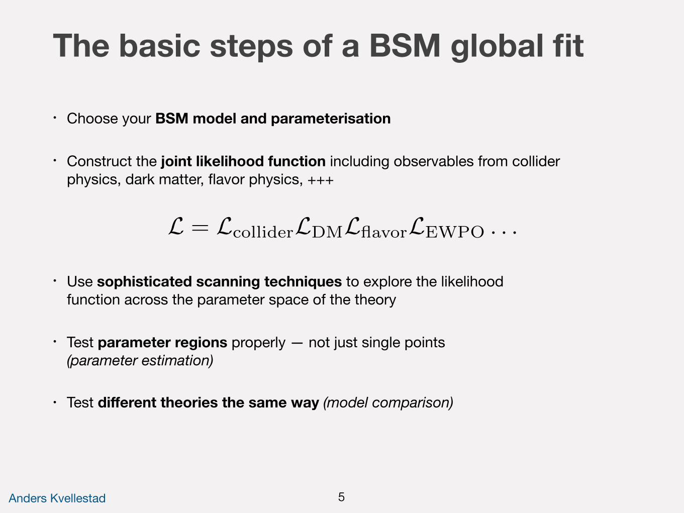
The basic steps of a BSM global fit
• Choose your BSM model and parameterisation
• Construct the joint likelihood function including observables from collider physics, dark matter, flavor physics, +++
• Use sophisticated scanning techniques to explore the likelihood function across the parameter space of the theory
• Test parameter regions properly — not just single points (parameter estimation)
• Test different theories the same way (model comparison)
L = LcolliderLDMLflavorLEWPO . . .
5
Anders Kvellestad 6
θ1
θ2
θ3
• L(θ)
• L(θ)
• L(θ)
• L(θ)
• L(θ)
• L(θ)• L(θ)
• L(θ)
• L(θ)
• L(θ)
• L(θ)
• L(θ)
• L(θ)• L(θ)
• L(θ)• L(θ)
• L(θ)
• L(θ)
• L(θ)• L(θ)• L(θ)• L(θ)
• L(θ)• L(θ)
• L(θ) • L(θ)• L(θ)
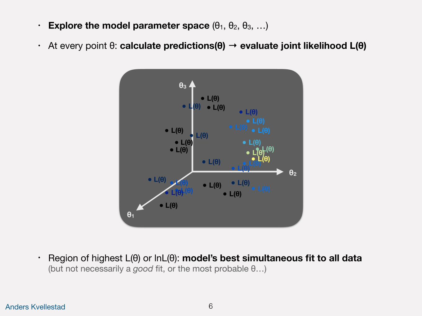
• Region of highest L(θ) or lnL(θ): model’s best simultaneous fit to all data(but not necessarily a good fit, or the most probable θ…)
• Explore the model parameter space (θ1, θ2, θ3, …)
• At every point θ: calculate predictions(θ) → evaluate joint likelihood L(θ)
Anders Kvellestad 7
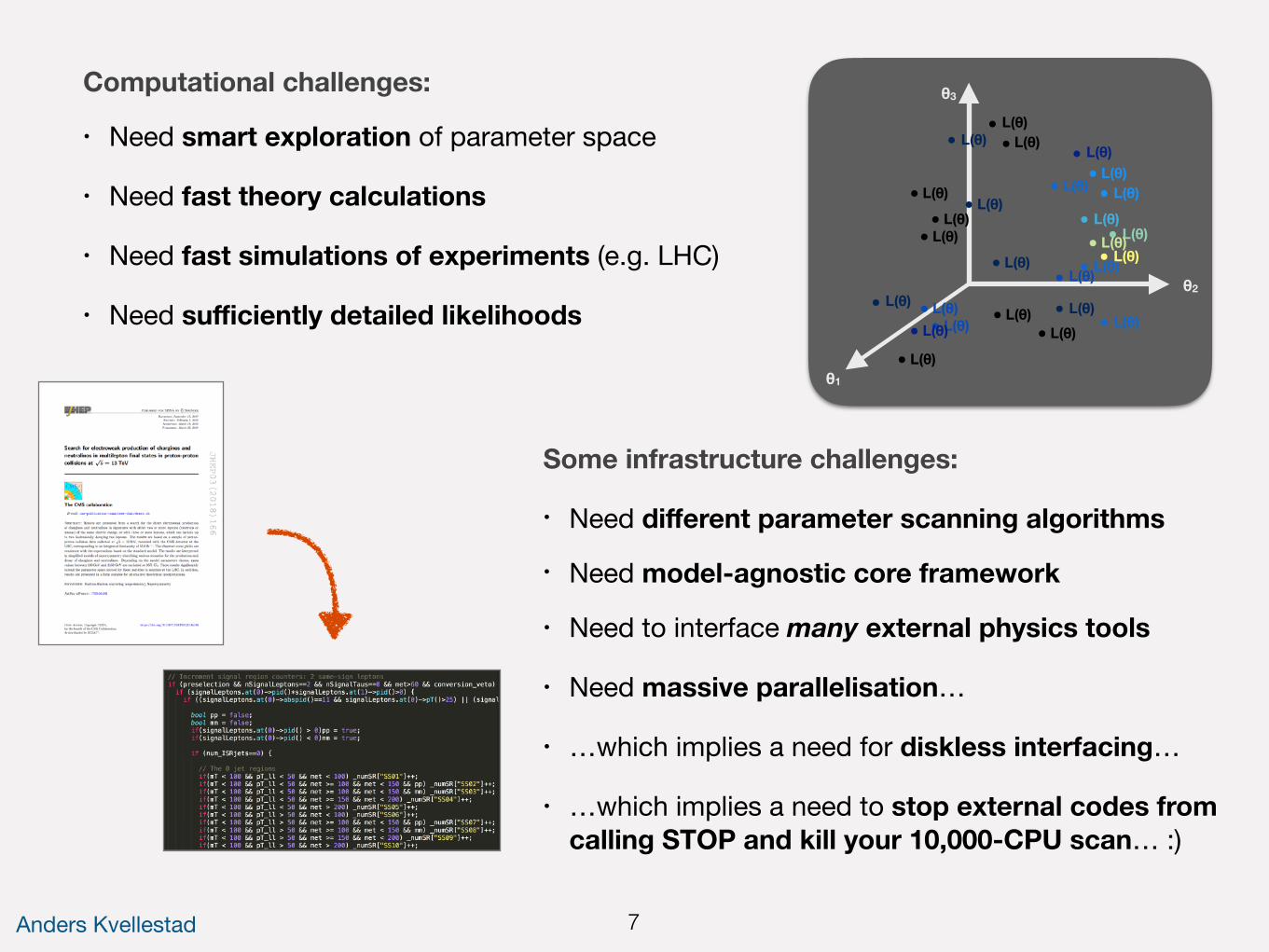
Computational challenges:
• Need smart exploration of parameter space
• Need fast theory calculations
• Need fast simulations of experiments (e.g. LHC)
• Need sufficiently detailed likelihoods
θ1
θ2
θ3
• L(θ)
• L(θ)
• L(θ)
• L(θ)
• L(θ)
• L(θ)• L(θ)
• L(θ)
• L(θ)
• L(θ)
• L(θ)
• L(θ)
• L(θ)• L(θ)
• L(θ)• L(θ)
• L(θ)
• L(θ)
• L(θ) • L(θ)• L(θ)• L(θ)
• L(θ)• L(θ)
• L(θ) • L(θ)• L(θ)
Some infrastructure challenges:
• Need different parameter scanning algorithms
• Need model-agnostic core framework
• Need to interface many external physics tools
• Need massive parallelisation…
• …which implies a need for diskless interfacing…
• …which implies a need to stop external codes from calling STOP and kill your 10,000-CPU scan… :)
Anders Kvellestad 8
2. GAMBIT
G AM B I T
Anders Kvellestad 9
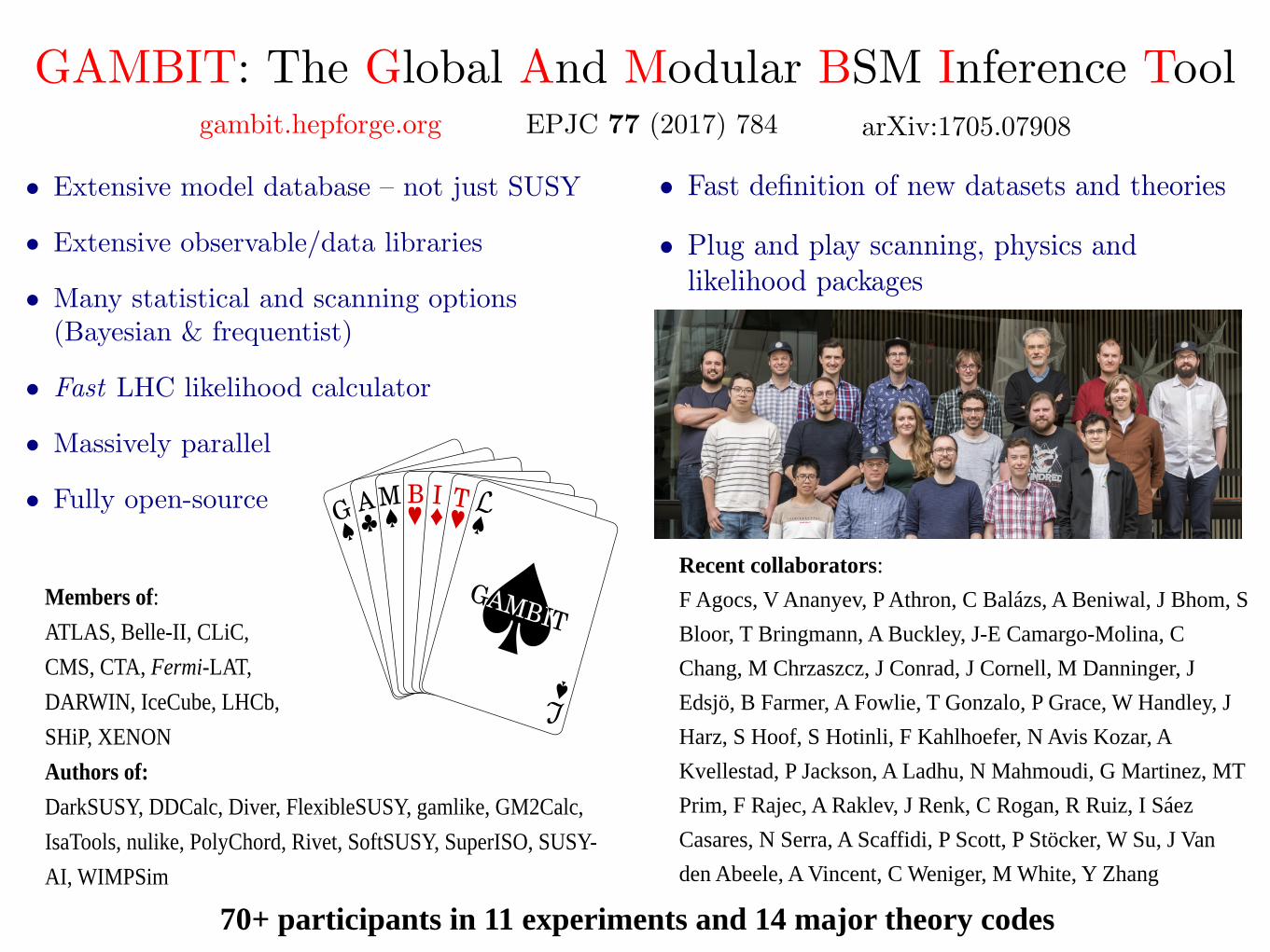
G AM B I T
Recent collaborators:F Agocs, V Ananyev, P Athron, C Balázs, A Beniwal, J Bhom, S Bloor, T Bringmann, A Buckley, J-E Camargo-Molina, C Chang, M Chrzaszcz, J Conrad, J Cornell, M Danninger, J Edsjö, B Farmer, A Fowlie, T Gonzalo, P Grace, W Handley, J Harz, S Hoof, S Hotinli, F Kahlhoefer, N Avis Kozar, A Kvellestad, P Jackson, A Ladhu, N Mahmoudi, G Martinez, MT Prim, F Rajec, A Raklev, J Renk, C Rogan, R Ruiz, I Sáez Casares, N Serra, A Scaffidi, P Scott, P Stöcker, W Su, J Van den Abeele, A Vincent, C Weniger, M White, Y Zhang
Members of:ATLAS, Belle-II, CLiC, CMS, CTA, Fermi-LAT, DARWIN, IceCube, LHCb, SHiP, XENONAuthors of:DarkSUSY, DDCalc, Diver, FlexibleSUSY, gamlike, GM2Calc, IsaTools, nulike, PolyChord, Rivet, SoftSUSY, SuperISO, SUSY-AI, WIMPSim
70+ participants in 11 experiments and 14 major theory codes
G AM B I TA. Kvellestad 10
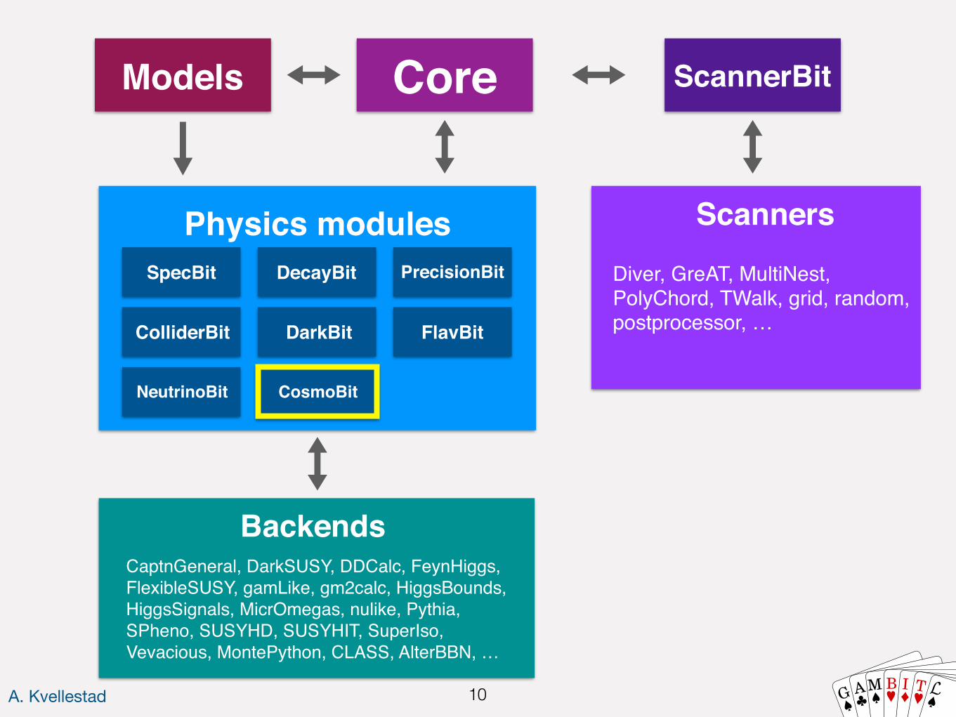
Models Core ScannerBit
CaptnGeneral, DarkSUSY, DDCalc, FeynHiggs, FlexibleSUSY, gamLike, gm2calc, HiggsBounds, HiggsSignals, MicrOmegas, nulike, Pythia, SPheno, SUSYHD, SUSYHIT, SuperIso, Vevacious, MontePython, CLASS, AlterBBN, …
Backends
Diver, GreAT, MultiNest, PolyChord, TWalk, grid, random, postprocessor, …
Scanners
ColliderBit DarkBit FlavBit
SpecBit DecayBit PrecisionBit
Physics modules
NeutrinoBit CosmoBit
Anders Kvellestad 11
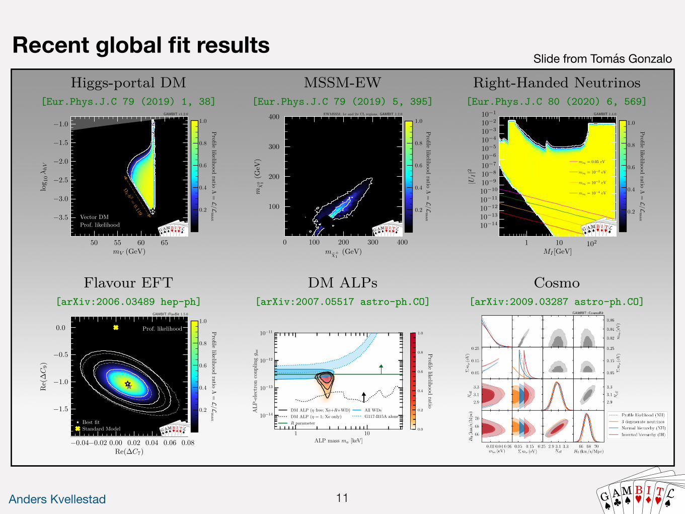
ExamplesHiggs-portal DM
[Eur.Phys.J.C 79 (2019) 1, 38]
★
➤
➤
GAMBIT v1.2.0
G AM B I T
⌦V h 2
=0.119
�3.5
�3.0
�2.5
�2.0
�1.5
�1.0
log 1
0�hV
Profi
lelikelih
oodratio
⇤=
L/L
max
50 55 60 65mV (GeV)
0.2
0.4
0.6
0.8
1.0
Vector DMProf. likelihood
Flavour EFT[arXiv:2006.03489 hep-ph]
★★
✚✖
✚✖★
Standard ModelBest fit
GAMBIT::FlavBit 1.5.0
G AM B I T
�1.5
�1.0
�0.5
0.0
Re(�C
9)
Profi
lelikelih
oodratio
⇤=
L/L
max
�0.04�0.02 0.00 0.02 0.04 0.06 0.08Re(�C7)
0.2
0.4
0.6
0.8
1.0Prof. likelihood
MSSM-EW[Eur.Phys.J.C 79 (2019) 5, 395]
★
EWMSSM. 1� and 2� CL regions. GAMBIT 1.2.0
G AM B I T
100
200
300
400
m�̃0 1(G
eV)
0 100 200 300 400m�̃+
1(GeV)
Profi
lelikelih
oodratio
⇤=
L/L
max
0.2
0.4
0.6
0.8
1.0
DM ALPs[arXiv:2007.05517 astro-ph.CO]
1 10ALP mass ma [keV]
10≠14
10≠13
10≠12
10≠11
ALP-
elect
ron
coup
lingg a
e
DM ALP (� free; Xe+R+WD)DM ALP (� = 1; Xe only)R parameter
All WDsG117-B15A alone
0.0
0.2
0.4
0.6
0.8
1.0
Profilelikelihood
ratio
Right-Handed Neutrinos[Eur.Phys.J.C 80 (2020) 6, 569]
GAMBIT 1.4.0
G AM B I T10�1410�1310�1210�1110�1010�910�810�710�610�510�410�310�210�1
|UI|2
Profi
lelikelih
oodratio
⇤=
L/L
max
1 10 102
MI [GeV]
0.2
0.4
0.6
0.8
1.0
m⌫0 = 0.05 eV
m⌫0 = 10�2 eV
m⌫0 = 10�3 eV
m⌫0 = 10�4 eV
Cosmo[arXiv:2009.03287 astro-ph.CO]
T. Gonzalo (Monash U) GAMBIT Tools 2020, 6/11/20 9 / 14
G AM B I T
Recent global fit resultsSlide from Tomás Gonzalo
Anders Kvellestad 12 G AM B I T
GAMBIT clearly works as a general framework for global fits…
…but how much work does it take to set up GAMBIT to study a new model?
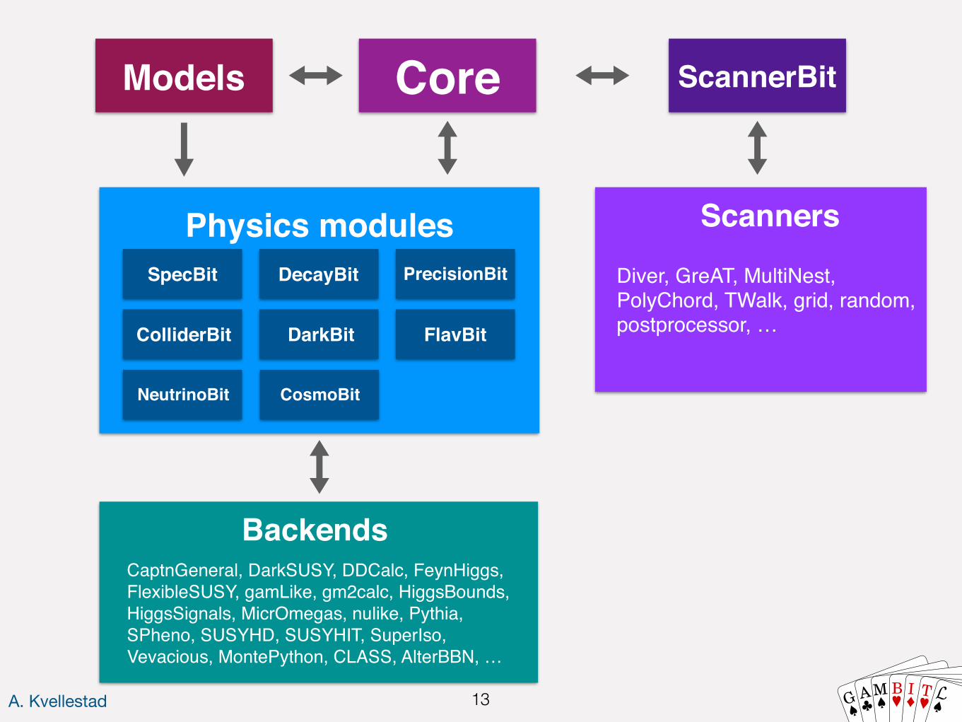
G AM B I TA. Kvellestad 13
Models Core ScannerBit
CaptnGeneral, DarkSUSY, DDCalc, FeynHiggs, FlexibleSUSY, gamLike, gm2calc, HiggsBounds, HiggsSignals, MicrOmegas, nulike, Pythia, SPheno, SUSYHD, SUSYHIT, SuperIso, Vevacious, MontePython, CLASS, AlterBBN, …
Backends
Diver, GreAT, MultiNest, PolyChord, TWalk, grid, random, postprocessor, …
Scanners
ColliderBit DarkBit FlavBit
SpecBit DecayBit PrecisionBit
Physics modules
NeutrinoBit CosmoBit

G AM B I TA. Kvellestad 14
Models Core ScannerBit
CaptnGeneral, DarkSUSY, DDCalc, FeynHiggs, FlexibleSUSY, gamLike, gm2calc, HiggsBounds, HiggsSignals, MicrOmegas, nulike, Pythia, SPheno, SUSYHD, SUSYHIT, SuperIso, Vevacious, MontePython, CLASS, AlterBBN, …
Backends
Diver, GreAT, MultiNest, PolyChord, TWalk, grid, random, postprocessor, …
Scanners
ColliderBit DarkBit FlavBit
SpecBit DecayBit PrecisionBit
Physics modules
NeutrinoBit CosmoBit
• This part is completely model independent
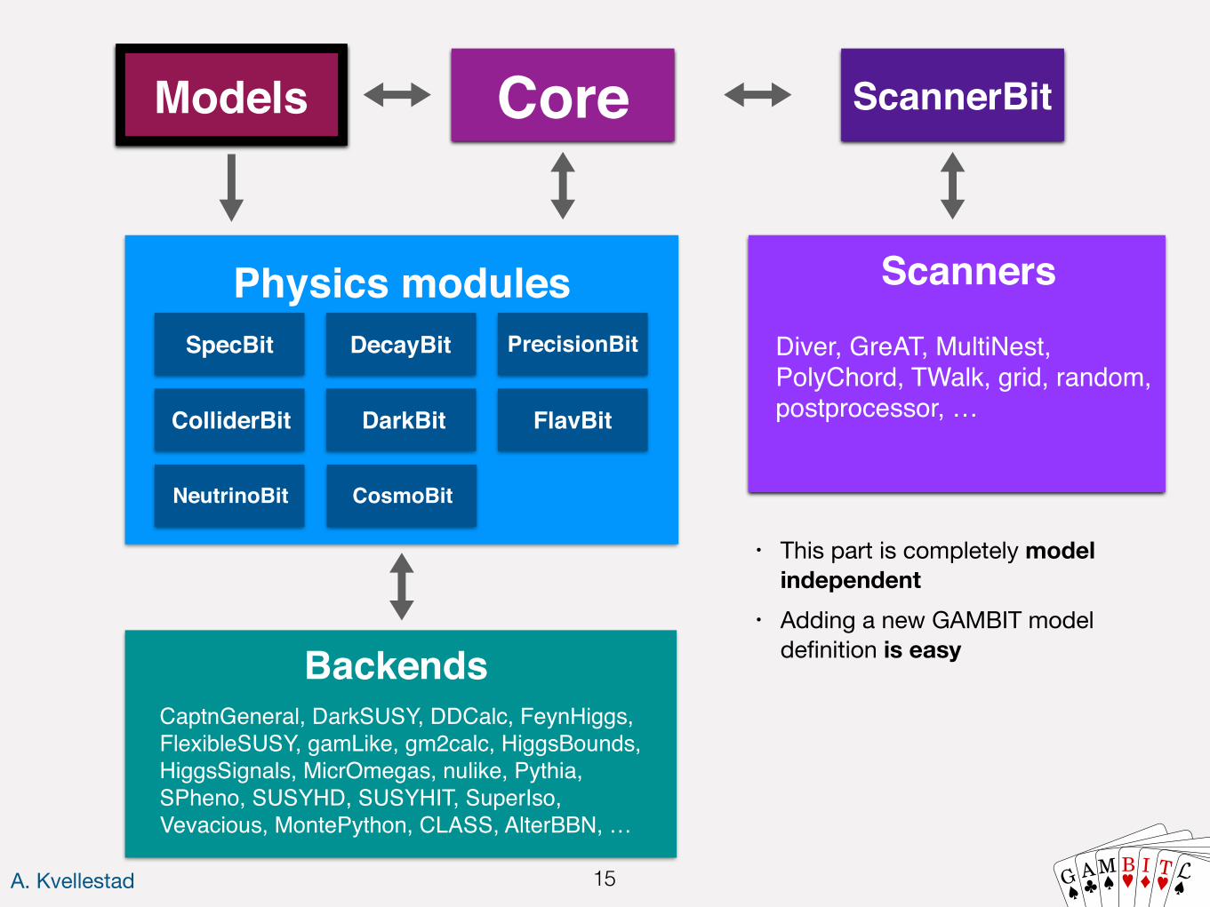
G AM B I TA. Kvellestad 15
Models Core ScannerBit
CaptnGeneral, DarkSUSY, DDCalc, FeynHiggs, FlexibleSUSY, gamLike, gm2calc, HiggsBounds, HiggsSignals, MicrOmegas, nulike, Pythia, SPheno, SUSYHD, SUSYHIT, SuperIso, Vevacious, MontePython, CLASS, AlterBBN, …
Backends
Diver, GreAT, MultiNest, PolyChord, TWalk, grid, random, postprocessor, …
Scanners
ColliderBit DarkBit FlavBit
SpecBit DecayBit PrecisionBit
Physics modules
NeutrinoBit CosmoBit
• This part is completely model independent
• Adding a new GAMBIT model definition is easy
G AM B I TA. Kvellestad 16
Models Core ScannerBit
CaptnGeneral, DarkSUSY, DDCalc, FeynHiggs, FlexibleSUSY, gamLike, gm2calc, HiggsBounds, HiggsSignals, MicrOmegas, nulike, Pythia, SPheno, SUSYHD, SUSYHIT, SuperIso, Vevacious, MontePython, CLASS, AlterBBN, …
Backends
Diver, GreAT, MultiNest, PolyChord, TWalk, grid, random, postprocessor, …
Scanners
ColliderBit DarkBit FlavBit
SpecBit DecayBit PrecisionBit
Physics modules
NeutrinoBit CosmoBit
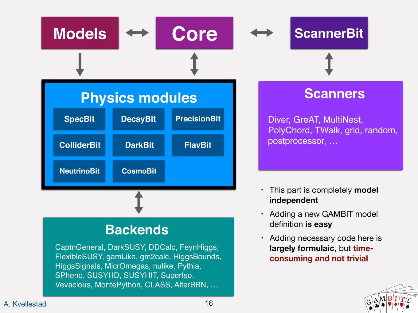
• This part is completely model independent
• Adding a new GAMBIT model definition is easy
• Adding necessary code here is largely formulaic, but time-consuming and not trivial
G AM B I TA. Kvellestad 17
Models Core ScannerBit
CaptnGeneral, DarkSUSY, DDCalc, FeynHiggs, FlexibleSUSY, gamLike, gm2calc, HiggsBounds, HiggsSignals, MicrOmegas, nulike, Pythia, SPheno, SUSYHD, SUSYHIT, SuperIso, Vevacious, MontePython, CLASS, AlterBBN, …
Backends
Diver, GreAT, MultiNest, PolyChord, TWalk, grid, random, postprocessor, …
Scanners
ColliderBit DarkBit FlavBit
SpecBit DecayBit PrecisionBit
Physics modules
NeutrinoBit CosmoBit
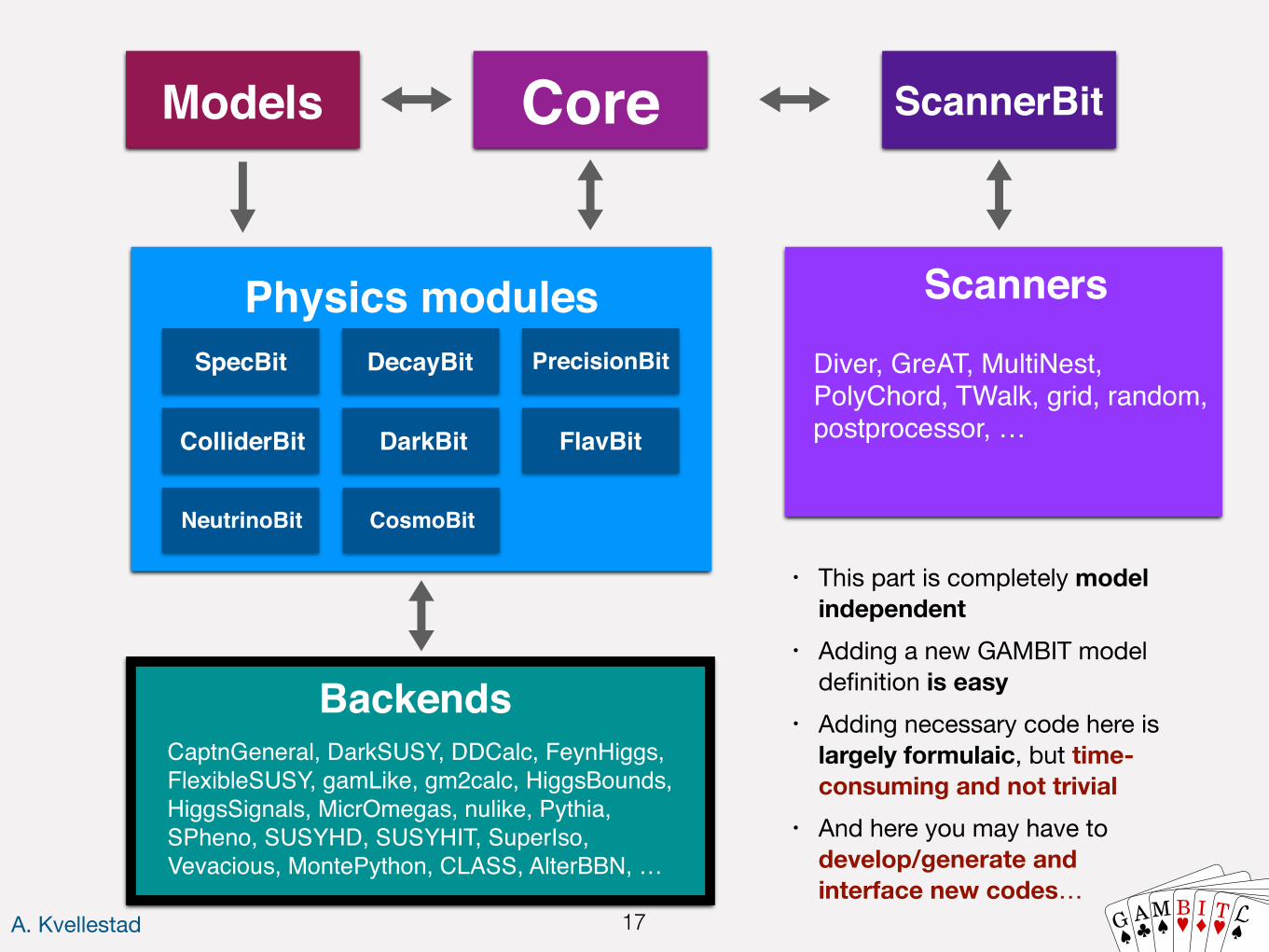
• This part is completely model independent
• Adding a new GAMBIT model definition is easy
• Adding necessary code here is largely formulaic, but time-consuming and not trivial
• And here you may have to develop/generate and interface new codes…
Anders Kvellestad 18
3. GUM:the GAMBIT Universal Model Machine
G AM B I T
S. Bloor, T. Gonzalo, P. Scott, C. Chang, et al
Anders Kvellestad 19 G AM B I T
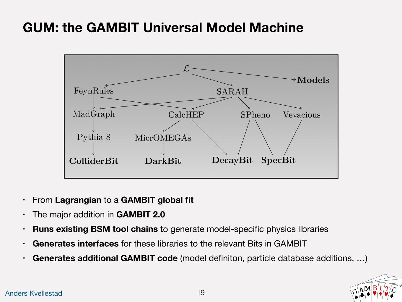
GUM: the GAMBIT Universal Model Machine
• From Lagrangian to a GAMBIT global fit• The major addition in GAMBIT 2.0• Runs existing BSM tool chains to generate model-specific physics libraries• Generates interfaces for these libraries to the relevant Bits in GAMBIT• Generates additional GAMBIT code (model definiton, particle database additions, …)
GUM
GUM interfaces LLT SARAH and FeynRules with GAMBITUses existing HEP toolchains
L
FeynRules SARAH
MadGraph CalcHEP SPheno
Pythia 8 MicrOMEGAs
Vevacious
ColliderBit DarkBit DecayBit SpecBit
Models
GAMBIT-compatible outputs from GUM
T. Gonzalo (Monash U) GAMBIT Tools 2020, 6/11/20 12 / 14
Anders Kvellestad 20 G AM B I T
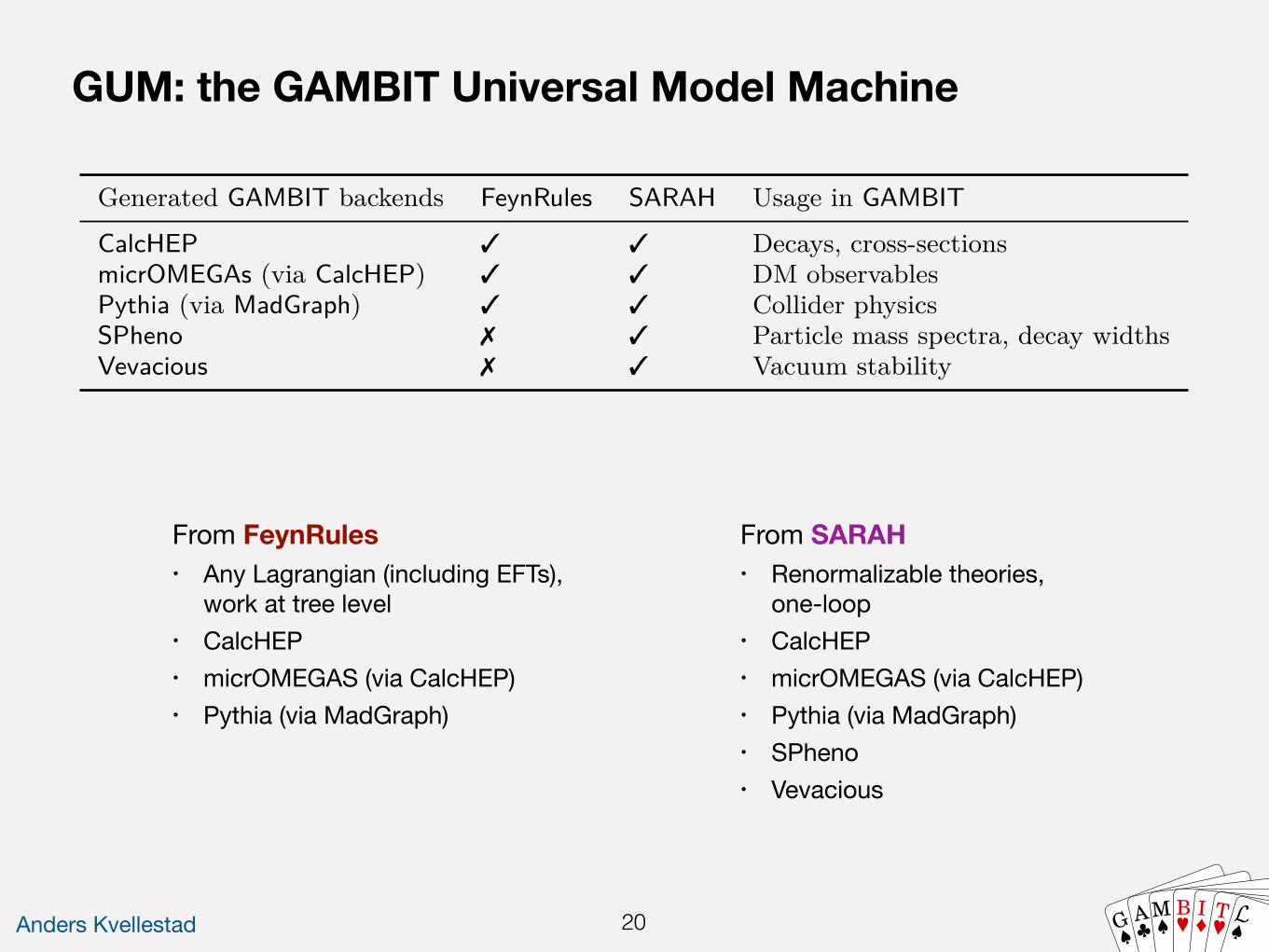
From FeynRules • Any Lagrangian (including EFTs),
work at tree level• CalcHEP• micrOMEGAS (via CalcHEP)• Pythia (via MadGraph)
GUM: the GAMBIT Universal Model Machine3
Generated GAMBIT backends FeynRules SARAH Usage in GAMBIT
CalcHEP 3 3 Decays, cross-sectionsmicrOMEGAs (via CalcHEP) 3 3 DM observablesPythia (via MadGraph) 3 3 Collider physicsSPheno 7 3 Particle mass spectra, decay widthsVevacious 7 3 Vacuum stability
Table 1: GAMBIT backends with GUM support and Lagrangian-level tools used to generate them. Apart from the external packageslisted, GUM also produces GAMBIT Core and physics module code tailored to the model and observables of interest.
Although the outputs of SARAH are more sophisti-cated than those of FeynRules, it also has limitations.Unlike in FeynRules, it is not generally possible to de-fine non-renormalisable theories or higher-dimensionale�ective theories in SARAH. We therefore provide inter-faces to both FeynRules and SARAH to allow the user toincorporate a vast range of theories into GAMBIT, frome�ective field theories (EFTs) via FeynRules to complexUV-complete theories in SARAH. We stress that if amodel can be implemented in SARAH, then the usershould use SARAH over FeynRules – both to use GAM-BIT to its full potential, and to perform more detailedphysics studies. The basic outputs available from GUMin each case are summarised in Table 1.1
This manual is organised as follows: in Sec. 2, we de-scribe the code structure and outputs of GUM. In Sec. 3we give usage details, including installation, the GUMfile, and particulars of FeynRules and SARAH modelfiles. In Sec. 4 we provide a worked example, where weuse GUM to add a simplified DM model to GAMBIT,and perform a quick statistical fit to DM observables.Finally, in Sec. 5, we discuss future extensions of GUMand summarise. We include details of the new GAMBITinterfaces to CalcHEP, Vevacious and SARAH-SPheno(the auto-generated version of SPheno created usingSARAH) in the Appendix.
GUM is open source and part of the GAMBIT 2.0release, available from gambit.hepforge.org under theterms of the standard 3-clause BSD license.2
2 Code design
GAMBIT consists of a set of Core software components,a sampling module ScannerBit [3], and a series of physicsmodules [4–9]. Each physics module is in charge of a
1Some readers will note the absence of FlexibleSUSY from thislist; this is due to the complex C++ templates used in Flexi-bleSUSY and the fact that supporting it fully as a backend inGAMBIT requires significant development of the classloadingabilities of the backend-on-a-stick script (BOSS) [1]. Once thischallenge has been overcome, future versions of GUM will alsogenerate code for FlexibleSUSY and its other flexi-bretheren.2http://opensource.org/licenses/BSD-3-Clause.
domain-specific subset of GAMBIT’s physical calcula-tions. GUM generates various snippets of code that itthen adds to parts of the GAMBIT Core, as well asto some of the physics modules, enabling GAMBIT toemploy the capabilities of those modules with the newmodel.
Within the Core, GUM adds code for any new parti-cles to the GAMBIT particle database, and code for thenew model to the GAMBIT models database, informingGAMBIT of the parameters of the new model so thatthey can be varied in a fit. GUM also generates interfaces(frontends) to the external codes (backends) that it isable to generate. The backends supported by GUM inthis manner are those listed as outputs in Table 1.
Within the physics modules, GUM writes new codefor the SpecBit [8] module, responsible for spectrumgeneration within GAMBIT, DecayBit [8], responsiblefor calculating the decays of particles, DarkBit [4], re-sponsible for DM observables, and ColliderBit [5], themodule that simulates hard-scattering, hadronisationand showering of particles at colliders, and implementssubsequent LHC analyses.
GUM is primarily written in Python, with the excep-tion of the Mathematica interface, which is written inC++ and accessed via Boost.Python.
Initially, GUM parses a .gum input file, using the con-tents to construct a singleton gum object. Details of theinput format can be found in Sec. 3.3. GUM then per-forms some simple sanity and consistency checks, suchas ensuring that if the user requests DM observables,they have also specified a DM candidate. GUM thenopens an interface to either FeynRules or SARAH viathe Wolfram Symbolic Transfer Protocol (WSTP), loadsthe FeynRules or SARAH model file that the user has re-quested into the Mathematica kernel, and performs someadditional sanity checks using the inbuilt diagnostics ofeach package.
Once GUM is satisfied with the FeynRules or SARAHmodel file, it extracts all physical particles, masses andparameters (e.g. mixings and couplings). The minimalinformation required to define a new particle is its mass,spin, color representation, PDG code, and electric charge(if non-self conjugate). For a parameter to be extracted,
From SARAH• Renormalizable theories,
one-loop• CalcHEP• micrOMEGAS (via CalcHEP)• Pythia (via MadGraph)• SPheno• Vevacious
Anders Kvellestad 21 G AM B I T
18
various means. In the absence of a spectrum genera-tor (e.g. SPheno, see below), almost all the parame-ters in ParameterDefinitions become model parameters.Only those with explicit dependencies on other param-eters are removed, i.e. those with the Dependence orDependenceSpheno fields. In addition, SARAH providestree-level relations for all masses, via TreeMass[particle_
name,EWSB], so even in the absence of a spectrum gener-ator, none of the particle masses become explicit modelparameters. For models with BSM states that mix to-gether into mass eigenstates6, the tree-level masses arenot used and an error is thrown to inform the user ofthe need to use a spectrum generator.
If the user elects in their .gum file to gener-ate any outputs from SARAH for specific backends,GUM requests that SARAH generate the respectivecode using the relevant SARAH commands. These areMakeCHep[] for CalcHEP and micrOMEGAs, MakeUFO[]for MadGraph/Pythia, MakeSPheno[] for SPheno andMakeVevacious[] for Vevacious.
When SPheno output is requested, GUM interactsfurther with SARAH in order to obtain all necessaryinformation for spectrum generation:
1. Replace parameters and masses with those inSPheno. The parameter names are obtained us-ing the SPhenoForm function operating on thelists listAllParametersAndVEVs and NewMassParameters.The particle masses are obtained just by using theSPhenoMass[particle_name] command.
2. Extract the names and default values of the pa-rameters in the MINPAR and EXTPAR blocks, as definedin the model file SPheno.m. For each of these, storethe boundary conditions, also from SPheno.m, thatmatch the MINPAR and EXTPAR parameters to those inthe parameter list. Note that as of GUM 1.0, onlythe boundary conditions in BoundaryLowScaleInputare parsed.
3. Remove from the parameter list those parametersthat will be fixed by the tadpole equations, as theyare not free parameters. These are collected from thelist ParametersToSolveTadpoles as defined in SPheno.m.
4. Get the names of the blocks, entries and parameternames for all SLHA input blocks ending in IN, e.g.HMIXIN, DSQIN, etc. SARAH provides this informationin the list CombindedBlocks.
5. Register the values of various flags needed toproperly set up the interface to SPheno. Theseare "SupersymmetricModel", "OnlyLowEnergySPheno","UseHiggs2LoopMSSM" and "SA‘AddOneLoopDecay".
6Technically this is done by checking if the PDG list for any ofthe BSM particles contains more than one entry.
4 A worked example
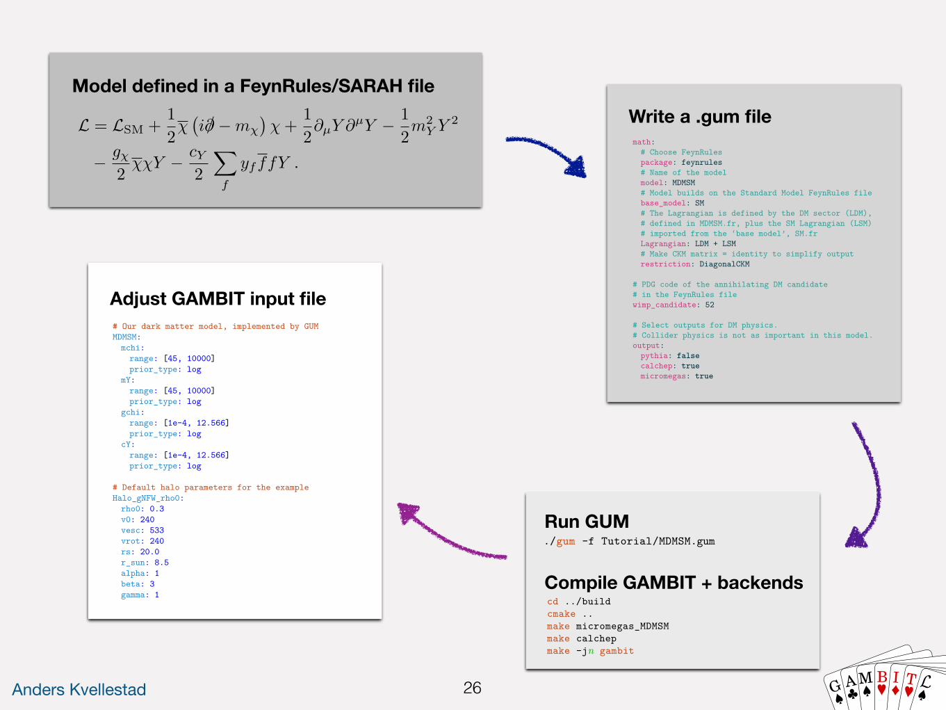
To demonstrate the process of adding a new model toGAMBIT with GUM, in this section we provide a simpleworked example. Here we use GUM to add a model toGAMBIT, perform a parameter scan, and plot the resultswith pippi [84]. This example is designed with ease of usein mind, and can be performed on a personal computerin a reasonable amount of time. For this reason we selecta simplified DM model, implemented in FeynRules.
In this example, we consider constraints from therelic density of dark matter, gamma-ray indirect detec-tion and traditional high-mass direct detection searches.It should be noted that this is an example, not a fullglobal scan, so we do not use all of the informationavailable to us – a real global fit of this model wouldconsider nuisance parameters relevant to DM, as wellas a full set of complementary likelihoods such as fromother indirect DM searches, low-mass direct detectionsearches, and cosmology.
The FeynRules model file, .gum file, GAMBIT inputfile and pip file used in this example can be found withinthe Tutorial folder in GUM.
4.1 The model
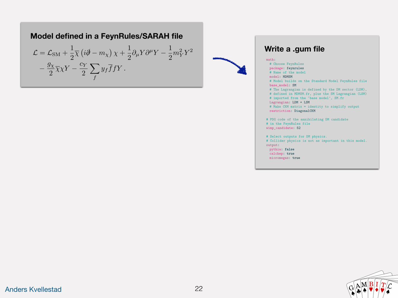
The model is a simplified DM model, where the Stan-dard Model is extended by a Majorana fermion ‰ actingas DM, and a scalar mediator Y with a Yukawa-typecoupling to all SM fermions, in order to adhere to min-imal flavour violation. The DM particle is kept stableby a Z2 symmetry under which it is odd, ‰ æ ≠‰, andall other particles are even. Both ‰ and Y are singletsunder the SM gauge group.
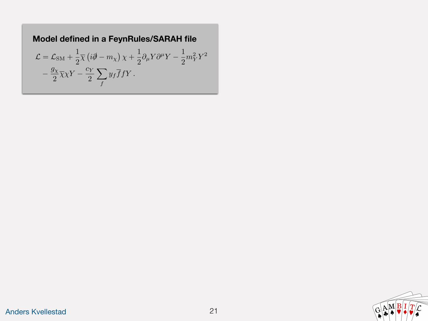
Here, we assume that any mixing between Y and theSM Higgs is small and can be neglected. This model hasbeen previously considered in e.g. [85, 86] and is alsoone of the benchmark simplified models used in LHCsearches [87–89]. The model Lagrangian is
L = LSM + 12‰
!i /̂ ≠ m‰
"‰ + 1
2ˆµY ˆµY ≠ 12m2
Y Y 2
≠ g‰
2 ‰‰Y ≠ cY
2ÿ
f
yf ffY . (1)
Note that this theory is not SU(2)L invariant. Onepossibility for a ‘realistic’ model involves Y -Higgs mix-ing, which justifies choosing the Y ff couplings to beproportional to the SM Yukawas yf .
The free parameters of the model are simply thedark sector masses and couplings, {m‰, mY , cY , g‰}. Inthis example we follow the FeynRules pathway, workingat tree level.
Model defined in a FeynRules/SARAH file
Anders Kvellestad 22 G AM B I T
Write a .gum file
19
4.2 The .gum file
Firstly, we need to add the FeynRules model file tothe GUM directory. The model is named ‘MDMSM’(Majorana DM, scalar mediator). Starting in the GUMroot directory, we first create the directory that themodel will live in, and move the example file from theTutorial folder to the GUM directory:
mkdir Models/MDMSMcp Tutorial/MDMSM.fr Models/MDMSM/
As we are working with FeynRules, the only backendsthat we are able to create output for are CalcHEP, mi-crOMEGAs and MadGraph/Pythia. For the sake of speed,in this tutorial we will not include any constraints fromcollider physics. This is also a reasonable approximation,as for the mass range that we consider here, the con-straints from e.g. monojet, dijet and dilepton searchesare subleading (see e.g. Ref. [85] and Appendix A). Wetherefore set pythia:false. The contents of the supplied.gum file are simple:
math:# Choose FeynRulespackage: feynrules# Name of the modelmodel: MDMSM# Model builds on the Standard Model FeynRules filebase_model: SM# The Lagrangian is defined by the DM sector (LDM),# defined in MDMSM.fr, plus the SM Lagrangian (LSM)# imported from the ‘base model’, SM.frLagrangian: LDM + LSM# Make CKM matrix = identity to simplify outputrestriction: DiagonalCKM
# PDG code of the annihilating DM candidate# in the FeynRules filewimp_candidate: 52
# Select outputs for DM physics.# Collider physics is not as important in this model.output:
pythia: falsecalchep: truemicromegas: true
Note the selection of the PDG code of the DM particleas 52, so that if we were to use Pythia, ‰ would becorrectly identified as invisible.
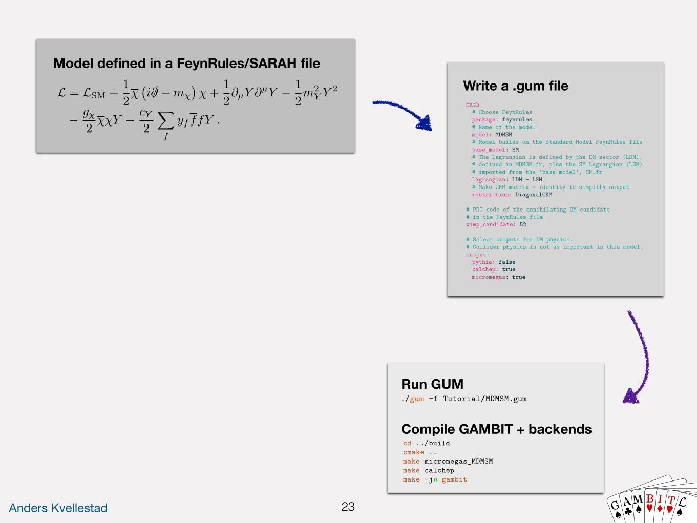
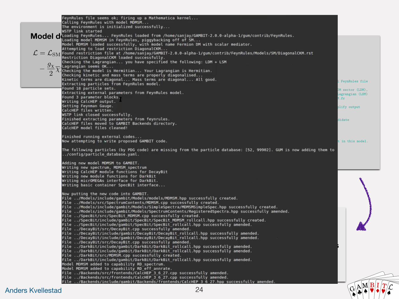
We can run this from the GUM directory,
./gum -f Tutorial/MDMSM.gum
and GUM will automatically create all code needed toperform a fit using GAMBIT. On a laptop with an IntelCore i5 processor, GUM takes about a minute to run.All that remains now is to (re)compile the relevantbackends and GAMBIT, and the new model will be fullyimplemented, and ready to scan. GUM prints a set of
suggested build commands to standard output to buildthe new backends and GAMBIT itself. Starting from thegum directory, these arecd ../buildcmake ..make micromegas_MDMSMmake calchepmake -jn gambit
where n specifies the number of processes to use whenbuilding.
Note that GUM does not adjust any CMake flagsused in previous GAMBIT compilations, so the abovecommands assume that the user has already configuredGAMBIT appropriately and built any relevant samplersbefore running GUM. A user wishing to instead configureand build GAMBIT from scratch after running GUM,in order to e.g. run the example scan of Sec. 4 usingdi�erential evolution sampling and MPI parallelisation,would need to instead docd buildcmake -D WITH_MPI=ON ..make divercmake ..make micromegas_MDMSMmake calchepmake gamlikemake ddcalcmake -jn gambit
For more thorough CMake instructions, see the READMEin the gum/Tutorial, and CMAKE_FLAGS.md in the GAMBITroot directory.
4.3 Phenomenology and Constraints
The constraints that we will consider for this model areentirely in the DM sector, as those from colliders areless severe (collider constraints are given in AppendixA). The dark matter constraint are:– Relic abundance: computed by micrOMEGAs, and
employed as an upper bound, in the spirit of e�ectiveDM models.
– Direct detection: rates computed by micrOMEGAs,likelihoods from XENON1T 2018 [90] and LUX2016 [91], as computed with DDCalc [4, 14, 15].
– Indirect detection: Fermi-LAT constraints fromgamma-ray observations of dwarf spheroidal galaxies(dSphs). Tree level cross-sections are computed byCalcHEP, “ ray yields are consequently computed viaDarkSUSY [92, 93], and the constraints are appliedby gamLike [4].As the relic density constraint is imposed only as
an upper bound, we rescale all DM observables by thefraction of DM, f = œ‰/œDM.
18
various means. In the absence of a spectrum genera-tor (e.g. SPheno, see below), almost all the parame-ters in ParameterDefinitions become model parameters.Only those with explicit dependencies on other param-eters are removed, i.e. those with the Dependence orDependenceSpheno fields. In addition, SARAH providestree-level relations for all masses, via TreeMass[particle_
name,EWSB], so even in the absence of a spectrum gener-ator, none of the particle masses become explicit modelparameters. For models with BSM states that mix to-gether into mass eigenstates6, the tree-level masses arenot used and an error is thrown to inform the user ofthe need to use a spectrum generator.
If the user elects in their .gum file to gener-ate any outputs from SARAH for specific backends,GUM requests that SARAH generate the respectivecode using the relevant SARAH commands. These areMakeCHep[] for CalcHEP and micrOMEGAs, MakeUFO[]for MadGraph/Pythia, MakeSPheno[] for SPheno andMakeVevacious[] for Vevacious.
When SPheno output is requested, GUM interactsfurther with SARAH in order to obtain all necessaryinformation for spectrum generation:
1. Replace parameters and masses with those inSPheno. The parameter names are obtained us-ing the SPhenoForm function operating on thelists listAllParametersAndVEVs and NewMassParameters.The particle masses are obtained just by using theSPhenoMass[particle_name] command.
2. Extract the names and default values of the pa-rameters in the MINPAR and EXTPAR blocks, as definedin the model file SPheno.m. For each of these, storethe boundary conditions, also from SPheno.m, thatmatch the MINPAR and EXTPAR parameters to those inthe parameter list. Note that as of GUM 1.0, onlythe boundary conditions in BoundaryLowScaleInputare parsed.
3. Remove from the parameter list those parametersthat will be fixed by the tadpole equations, as theyare not free parameters. These are collected from thelist ParametersToSolveTadpoles as defined in SPheno.m.
4. Get the names of the blocks, entries and parameternames for all SLHA input blocks ending in IN, e.g.HMIXIN, DSQIN, etc. SARAH provides this informationin the list CombindedBlocks.
5. Register the values of various flags needed toproperly set up the interface to SPheno. Theseare "SupersymmetricModel", "OnlyLowEnergySPheno","UseHiggs2LoopMSSM" and "SA‘AddOneLoopDecay".
6Technically this is done by checking if the PDG list for any ofthe BSM particles contains more than one entry.
4 A worked example
To demonstrate the process of adding a new model toGAMBIT with GUM, in this section we provide a simpleworked example. Here we use GUM to add a model toGAMBIT, perform a parameter scan, and plot the resultswith pippi [84]. This example is designed with ease of usein mind, and can be performed on a personal computerin a reasonable amount of time. For this reason we selecta simplified DM model, implemented in FeynRules.
In this example, we consider constraints from therelic density of dark matter, gamma-ray indirect detec-tion and traditional high-mass direct detection searches.It should be noted that this is an example, not a fullglobal scan, so we do not use all of the informationavailable to us – a real global fit of this model wouldconsider nuisance parameters relevant to DM, as wellas a full set of complementary likelihoods such as fromother indirect DM searches, low-mass direct detectionsearches, and cosmology.
The FeynRules model file, .gum file, GAMBIT inputfile and pip file used in this example can be found withinthe Tutorial folder in GUM.
4.1 The model
The model is a simplified DM model, where the Stan-dard Model is extended by a Majorana fermion ‰ actingas DM, and a scalar mediator Y with a Yukawa-typecoupling to all SM fermions, in order to adhere to min-imal flavour violation. The DM particle is kept stableby a Z2 symmetry under which it is odd, ‰ æ ≠‰, andall other particles are even. Both ‰ and Y are singletsunder the SM gauge group.
Here, we assume that any mixing between Y and theSM Higgs is small and can be neglected. This model hasbeen previously considered in e.g. [85, 86] and is alsoone of the benchmark simplified models used in LHCsearches [87–89]. The model Lagrangian is
L = LSM + 12‰
!i /̂ ≠ m‰
"‰ + 1
2ˆµY ˆµY ≠ 12m2
Y Y 2
≠ g‰
2 ‰‰Y ≠ cY
2ÿ
f
yf ffY . (1)
Note that this theory is not SU(2)L invariant. Onepossibility for a ‘realistic’ model involves Y -Higgs mix-ing, which justifies choosing the Y ff couplings to beproportional to the SM Yukawas yf .
The free parameters of the model are simply thedark sector masses and couplings, {m‰, mY , cY , g‰}. Inthis example we follow the FeynRules pathway, workingat tree level.
Model defined in a FeynRules/SARAH file
Anders Kvellestad 23 G AM B I T
Write a .gum file
Run GUM
19
4.2 The .gum file
Firstly, we need to add the FeynRules model file tothe GUM directory. The model is named ‘MDMSM’(Majorana DM, scalar mediator). Starting in the GUMroot directory, we first create the directory that themodel will live in, and move the example file from theTutorial folder to the GUM directory:
mkdir Models/MDMSMcp Tutorial/MDMSM.fr Models/MDMSM/
As we are working with FeynRules, the only backendsthat we are able to create output for are CalcHEP, mi-crOMEGAs and MadGraph/Pythia. For the sake of speed,in this tutorial we will not include any constraints fromcollider physics. This is also a reasonable approximation,as for the mass range that we consider here, the con-straints from e.g. monojet, dijet and dilepton searchesare subleading (see e.g. Ref. [85] and Appendix A). Wetherefore set pythia:false. The contents of the supplied.gum file are simple:
math:# Choose FeynRulespackage: feynrules# Name of the modelmodel: MDMSM# Model builds on the Standard Model FeynRules filebase_model: SM# The Lagrangian is defined by the DM sector (LDM),# defined in MDMSM.fr, plus the SM Lagrangian (LSM)# imported from the ‘base model’, SM.frLagrangian: LDM + LSM# Make CKM matrix = identity to simplify outputrestriction: DiagonalCKM
# PDG code of the annihilating DM candidate# in the FeynRules filewimp_candidate: 52
# Select outputs for DM physics.# Collider physics is not as important in this model.output:
pythia: falsecalchep: truemicromegas: true
Note the selection of the PDG code of the DM particleas 52, so that if we were to use Pythia, ‰ would becorrectly identified as invisible.
We can run this from the GUM directory,
./gum -f Tutorial/MDMSM.gum
and GUM will automatically create all code needed toperform a fit using GAMBIT. On a laptop with an IntelCore i5 processor, GUM takes about a minute to run.All that remains now is to (re)compile the relevantbackends and GAMBIT, and the new model will be fullyimplemented, and ready to scan. GUM prints a set of
suggested build commands to standard output to buildthe new backends and GAMBIT itself. Starting from thegum directory, these arecd ../buildcmake ..make micromegas_MDMSMmake calchepmake -jn gambit
where n specifies the number of processes to use whenbuilding.
Note that GUM does not adjust any CMake flagsused in previous GAMBIT compilations, so the abovecommands assume that the user has already configuredGAMBIT appropriately and built any relevant samplersbefore running GUM. A user wishing to instead configureand build GAMBIT from scratch after running GUM,in order to e.g. run the example scan of Sec. 4 usingdi�erential evolution sampling and MPI parallelisation,would need to instead docd buildcmake -D WITH_MPI=ON ..make divercmake ..make micromegas_MDMSMmake calchepmake gamlikemake ddcalcmake -jn gambit
For more thorough CMake instructions, see the READMEin the gum/Tutorial, and CMAKE_FLAGS.md in the GAMBITroot directory.
4.3 Phenomenology and Constraints
The constraints that we will consider for this model areentirely in the DM sector, as those from colliders areless severe (collider constraints are given in AppendixA). The dark matter constraint are:– Relic abundance: computed by micrOMEGAs, and
employed as an upper bound, in the spirit of e�ectiveDM models.
– Direct detection: rates computed by micrOMEGAs,likelihoods from XENON1T 2018 [90] and LUX2016 [91], as computed with DDCalc [4, 14, 15].
– Indirect detection: Fermi-LAT constraints fromgamma-ray observations of dwarf spheroidal galaxies(dSphs). Tree level cross-sections are computed byCalcHEP, “ ray yields are consequently computed viaDarkSUSY [92, 93], and the constraints are appliedby gamLike [4].As the relic density constraint is imposed only as
an upper bound, we rescale all DM observables by thefraction of DM, f = œ‰/œDM.
Compile GAMBIT + backends
19
4.2 The .gum file
Firstly, we need to add the FeynRules model file tothe GUM directory. The model is named ‘MDMSM’(Majorana DM, scalar mediator). Starting in the GUMroot directory, we first create the directory that themodel will live in, and move the example file from theTutorial folder to the GUM directory:
mkdir Models/MDMSMcp Tutorial/MDMSM.fr Models/MDMSM/
As we are working with FeynRules, the only backendsthat we are able to create output for are CalcHEP, mi-crOMEGAs and MadGraph/Pythia. For the sake of speed,in this tutorial we will not include any constraints fromcollider physics. This is also a reasonable approximation,as for the mass range that we consider here, the con-straints from e.g. monojet, dijet and dilepton searchesare subleading (see e.g. Ref. [85] and Appendix A). Wetherefore set pythia:false. The contents of the supplied.gum file are simple:
math:# Choose FeynRulespackage: feynrules# Name of the modelmodel: MDMSM# Model builds on the Standard Model FeynRules filebase_model: SM# The Lagrangian is defined by the DM sector (LDM),# defined in MDMSM.fr, plus the SM Lagrangian (LSM)# imported from the ‘base model’, SM.frLagrangian: LDM + LSM# Make CKM matrix = identity to simplify outputrestriction: DiagonalCKM
# PDG code of the annihilating DM candidate# in the FeynRules filewimp_candidate: 52
# Select outputs for DM physics.# Collider physics is not as important in this model.output:
pythia: falsecalchep: truemicromegas: true
Note the selection of the PDG code of the DM particleas 52, so that if we were to use Pythia, ‰ would becorrectly identified as invisible.
We can run this from the GUM directory,
./gum -f Tutorial/MDMSM.gum
and GUM will automatically create all code needed toperform a fit using GAMBIT. On a laptop with an IntelCore i5 processor, GUM takes about a minute to run.All that remains now is to (re)compile the relevantbackends and GAMBIT, and the new model will be fullyimplemented, and ready to scan. GUM prints a set of
suggested build commands to standard output to buildthe new backends and GAMBIT itself. Starting from thegum directory, these arecd ../buildcmake ..make micromegas_MDMSMmake calchepmake -jn gambit
where n specifies the number of processes to use whenbuilding.
Note that GUM does not adjust any CMake flagsused in previous GAMBIT compilations, so the abovecommands assume that the user has already configuredGAMBIT appropriately and built any relevant samplersbefore running GUM. A user wishing to instead configureand build GAMBIT from scratch after running GUM,in order to e.g. run the example scan of Sec. 4 usingdi�erential evolution sampling and MPI parallelisation,would need to instead docd buildcmake -D WITH_MPI=ON ..make divercmake ..make micromegas_MDMSMmake calchepmake gamlikemake ddcalcmake -jn gambit
For more thorough CMake instructions, see the READMEin the gum/Tutorial, and CMAKE_FLAGS.md in the GAMBITroot directory.
4.3 Phenomenology and Constraints
The constraints that we will consider for this model areentirely in the DM sector, as those from colliders areless severe (collider constraints are given in AppendixA). The dark matter constraint are:– Relic abundance: computed by micrOMEGAs, and
employed as an upper bound, in the spirit of e�ectiveDM models.
– Direct detection: rates computed by micrOMEGAs,likelihoods from XENON1T 2018 [90] and LUX2016 [91], as computed with DDCalc [4, 14, 15].
– Indirect detection: Fermi-LAT constraints fromgamma-ray observations of dwarf spheroidal galaxies(dSphs). Tree level cross-sections are computed byCalcHEP, “ ray yields are consequently computed viaDarkSUSY [92, 93], and the constraints are appliedby gamLike [4].As the relic density constraint is imposed only as
an upper bound, we rescale all DM observables by thefraction of DM, f = œ‰/œDM.
18
various means. In the absence of a spectrum genera-tor (e.g. SPheno, see below), almost all the parame-ters in ParameterDefinitions become model parameters.Only those with explicit dependencies on other param-eters are removed, i.e. those with the Dependence orDependenceSpheno fields. In addition, SARAH providestree-level relations for all masses, via TreeMass[particle_
name,EWSB], so even in the absence of a spectrum gener-ator, none of the particle masses become explicit modelparameters. For models with BSM states that mix to-gether into mass eigenstates6, the tree-level masses arenot used and an error is thrown to inform the user ofthe need to use a spectrum generator.
If the user elects in their .gum file to gener-ate any outputs from SARAH for specific backends,GUM requests that SARAH generate the respectivecode using the relevant SARAH commands. These areMakeCHep[] for CalcHEP and micrOMEGAs, MakeUFO[]for MadGraph/Pythia, MakeSPheno[] for SPheno andMakeVevacious[] for Vevacious.
When SPheno output is requested, GUM interactsfurther with SARAH in order to obtain all necessaryinformation for spectrum generation:
1. Replace parameters and masses with those inSPheno. The parameter names are obtained us-ing the SPhenoForm function operating on thelists listAllParametersAndVEVs and NewMassParameters.The particle masses are obtained just by using theSPhenoMass[particle_name] command.
2. Extract the names and default values of the pa-rameters in the MINPAR and EXTPAR blocks, as definedin the model file SPheno.m. For each of these, storethe boundary conditions, also from SPheno.m, thatmatch the MINPAR and EXTPAR parameters to those inthe parameter list. Note that as of GUM 1.0, onlythe boundary conditions in BoundaryLowScaleInputare parsed.
3. Remove from the parameter list those parametersthat will be fixed by the tadpole equations, as theyare not free parameters. These are collected from thelist ParametersToSolveTadpoles as defined in SPheno.m.
4. Get the names of the blocks, entries and parameternames for all SLHA input blocks ending in IN, e.g.HMIXIN, DSQIN, etc. SARAH provides this informationin the list CombindedBlocks.
5. Register the values of various flags needed toproperly set up the interface to SPheno. Theseare "SupersymmetricModel", "OnlyLowEnergySPheno","UseHiggs2LoopMSSM" and "SA‘AddOneLoopDecay".
6Technically this is done by checking if the PDG list for any ofthe BSM particles contains more than one entry.
4 A worked example
To demonstrate the process of adding a new model toGAMBIT with GUM, in this section we provide a simpleworked example. Here we use GUM to add a model toGAMBIT, perform a parameter scan, and plot the resultswith pippi [84]. This example is designed with ease of usein mind, and can be performed on a personal computerin a reasonable amount of time. For this reason we selecta simplified DM model, implemented in FeynRules.
In this example, we consider constraints from therelic density of dark matter, gamma-ray indirect detec-tion and traditional high-mass direct detection searches.It should be noted that this is an example, not a fullglobal scan, so we do not use all of the informationavailable to us – a real global fit of this model wouldconsider nuisance parameters relevant to DM, as wellas a full set of complementary likelihoods such as fromother indirect DM searches, low-mass direct detectionsearches, and cosmology.
The FeynRules model file, .gum file, GAMBIT inputfile and pip file used in this example can be found withinthe Tutorial folder in GUM.
4.1 The model
The model is a simplified DM model, where the Stan-dard Model is extended by a Majorana fermion ‰ actingas DM, and a scalar mediator Y with a Yukawa-typecoupling to all SM fermions, in order to adhere to min-imal flavour violation. The DM particle is kept stableby a Z2 symmetry under which it is odd, ‰ æ ≠‰, andall other particles are even. Both ‰ and Y are singletsunder the SM gauge group.
Here, we assume that any mixing between Y and theSM Higgs is small and can be neglected. This model hasbeen previously considered in e.g. [85, 86] and is alsoone of the benchmark simplified models used in LHCsearches [87–89]. The model Lagrangian is
L = LSM + 12‰
!i /̂ ≠ m‰
"‰ + 1
2ˆµY ˆµY ≠ 12m2
Y Y 2
≠ g‰
2 ‰‰Y ≠ cY
2ÿ
f
yf ffY . (1)
Note that this theory is not SU(2)L invariant. Onepossibility for a ‘realistic’ model involves Y -Higgs mix-ing, which justifies choosing the Y ff couplings to beproportional to the SM Yukawas yf .
The free parameters of the model are simply thedark sector masses and couplings, {m‰, mY , cY , g‰}. Inthis example we follow the FeynRules pathway, workingat tree level.
Model defined in a FeynRules/SARAH file
Anders Kvellestad 24 G AM B I T
Write a .gum file
Run GUM
19
4.2 The .gum file
Firstly, we need to add the FeynRules model file tothe GUM directory. The model is named ‘MDMSM’(Majorana DM, scalar mediator). Starting in the GUMroot directory, we first create the directory that themodel will live in, and move the example file from theTutorial folder to the GUM directory:
mkdir Models/MDMSMcp Tutorial/MDMSM.fr Models/MDMSM/
As we are working with FeynRules, the only backendsthat we are able to create output for are CalcHEP, mi-crOMEGAs and MadGraph/Pythia. For the sake of speed,in this tutorial we will not include any constraints fromcollider physics. This is also a reasonable approximation,as for the mass range that we consider here, the con-straints from e.g. monojet, dijet and dilepton searchesare subleading (see e.g. Ref. [85] and Appendix A). Wetherefore set pythia:false. The contents of the supplied.gum file are simple:
math:# Choose FeynRulespackage: feynrules# Name of the modelmodel: MDMSM# Model builds on the Standard Model FeynRules filebase_model: SM# The Lagrangian is defined by the DM sector (LDM),# defined in MDMSM.fr, plus the SM Lagrangian (LSM)# imported from the ‘base model’, SM.frLagrangian: LDM + LSM# Make CKM matrix = identity to simplify outputrestriction: DiagonalCKM
# PDG code of the annihilating DM candidate# in the FeynRules filewimp_candidate: 52
# Select outputs for DM physics.# Collider physics is not as important in this model.output:
pythia: falsecalchep: truemicromegas: true
Note the selection of the PDG code of the DM particleas 52, so that if we were to use Pythia, ‰ would becorrectly identified as invisible.
We can run this from the GUM directory,
./gum -f Tutorial/MDMSM.gum
and GUM will automatically create all code needed toperform a fit using GAMBIT. On a laptop with an IntelCore i5 processor, GUM takes about a minute to run.All that remains now is to (re)compile the relevantbackends and GAMBIT, and the new model will be fullyimplemented, and ready to scan. GUM prints a set of
suggested build commands to standard output to buildthe new backends and GAMBIT itself. Starting from thegum directory, these arecd ../buildcmake ..make micromegas_MDMSMmake calchepmake -jn gambit
where n specifies the number of processes to use whenbuilding.
Note that GUM does not adjust any CMake flagsused in previous GAMBIT compilations, so the abovecommands assume that the user has already configuredGAMBIT appropriately and built any relevant samplersbefore running GUM. A user wishing to instead configureand build GAMBIT from scratch after running GUM,in order to e.g. run the example scan of Sec. 4 usingdi�erential evolution sampling and MPI parallelisation,would need to instead docd buildcmake -D WITH_MPI=ON ..make divercmake ..make micromegas_MDMSMmake calchepmake gamlikemake ddcalcmake -jn gambit
For more thorough CMake instructions, see the READMEin the gum/Tutorial, and CMAKE_FLAGS.md in the GAMBITroot directory.
4.3 Phenomenology and Constraints
The constraints that we will consider for this model areentirely in the DM sector, as those from colliders areless severe (collider constraints are given in AppendixA). The dark matter constraint are:– Relic abundance: computed by micrOMEGAs, and
employed as an upper bound, in the spirit of e�ectiveDM models.
– Direct detection: rates computed by micrOMEGAs,likelihoods from XENON1T 2018 [90] and LUX2016 [91], as computed with DDCalc [4, 14, 15].
– Indirect detection: Fermi-LAT constraints fromgamma-ray observations of dwarf spheroidal galaxies(dSphs). Tree level cross-sections are computed byCalcHEP, “ ray yields are consequently computed viaDarkSUSY [92, 93], and the constraints are appliedby gamLike [4].As the relic density constraint is imposed only as
an upper bound, we rescale all DM observables by thefraction of DM, f = œ‰/œDM.
Compile GAMBIT + backends
19
4.2 The .gum file
Firstly, we need to add the FeynRules model file tothe GUM directory. The model is named ‘MDMSM’(Majorana DM, scalar mediator). Starting in the GUMroot directory, we first create the directory that themodel will live in, and move the example file from theTutorial folder to the GUM directory:
mkdir Models/MDMSMcp Tutorial/MDMSM.fr Models/MDMSM/
As we are working with FeynRules, the only backendsthat we are able to create output for are CalcHEP, mi-crOMEGAs and MadGraph/Pythia. For the sake of speed,in this tutorial we will not include any constraints fromcollider physics. This is also a reasonable approximation,as for the mass range that we consider here, the con-straints from e.g. monojet, dijet and dilepton searchesare subleading (see e.g. Ref. [85] and Appendix A). Wetherefore set pythia:false. The contents of the supplied.gum file are simple:
math:# Choose FeynRulespackage: feynrules# Name of the modelmodel: MDMSM# Model builds on the Standard Model FeynRules filebase_model: SM# The Lagrangian is defined by the DM sector (LDM),# defined in MDMSM.fr, plus the SM Lagrangian (LSM)# imported from the ‘base model’, SM.frLagrangian: LDM + LSM# Make CKM matrix = identity to simplify outputrestriction: DiagonalCKM
# PDG code of the annihilating DM candidate# in the FeynRules filewimp_candidate: 52
# Select outputs for DM physics.# Collider physics is not as important in this model.output:
pythia: falsecalchep: truemicromegas: true
Note the selection of the PDG code of the DM particleas 52, so that if we were to use Pythia, ‰ would becorrectly identified as invisible.
We can run this from the GUM directory,
./gum -f Tutorial/MDMSM.gum
and GUM will automatically create all code needed toperform a fit using GAMBIT. On a laptop with an IntelCore i5 processor, GUM takes about a minute to run.All that remains now is to (re)compile the relevantbackends and GAMBIT, and the new model will be fullyimplemented, and ready to scan. GUM prints a set of
suggested build commands to standard output to buildthe new backends and GAMBIT itself. Starting from thegum directory, these arecd ../buildcmake ..make micromegas_MDMSMmake calchepmake -jn gambit
where n specifies the number of processes to use whenbuilding.
Note that GUM does not adjust any CMake flagsused in previous GAMBIT compilations, so the abovecommands assume that the user has already configuredGAMBIT appropriately and built any relevant samplersbefore running GUM. A user wishing to instead configureand build GAMBIT from scratch after running GUM,in order to e.g. run the example scan of Sec. 4 usingdi�erential evolution sampling and MPI parallelisation,would need to instead docd buildcmake -D WITH_MPI=ON ..make divercmake ..make micromegas_MDMSMmake calchepmake gamlikemake ddcalcmake -jn gambit
For more thorough CMake instructions, see the READMEin the gum/Tutorial, and CMAKE_FLAGS.md in the GAMBITroot directory.
4.3 Phenomenology and Constraints
The constraints that we will consider for this model areentirely in the DM sector, as those from colliders areless severe (collider constraints are given in AppendixA). The dark matter constraint are:– Relic abundance: computed by micrOMEGAs, and
employed as an upper bound, in the spirit of e�ectiveDM models.
– Direct detection: rates computed by micrOMEGAs,likelihoods from XENON1T 2018 [90] and LUX2016 [91], as computed with DDCalc [4, 14, 15].
– Indirect detection: Fermi-LAT constraints fromgamma-ray observations of dwarf spheroidal galaxies(dSphs). Tree level cross-sections are computed byCalcHEP, “ ray yields are consequently computed viaDarkSUSY [92, 93], and the constraints are appliedby gamLike [4].As the relic density constraint is imposed only as
an upper bound, we rescale all DM observables by thefraction of DM, f = œ‰/œDM.
19
4.2 The .gum file
Firstly, we need to add the FeynRules model file tothe GUM directory. The model is named ‘MDMSM’(Majorana DM, scalar mediator). Starting in the GUMroot directory, we first create the directory that themodel will live in, and move the example file from theTutorial folder to the GUM directory:
mkdir Models/MDMSMcp Tutorial/MDMSM.fr Models/MDMSM/
As we are working with FeynRules, the only backendsthat we are able to create output for are CalcHEP, mi-crOMEGAs and MadGraph/Pythia. For the sake of speed,in this tutorial we will not include any constraints fromcollider physics. This is also a reasonable approximation,as for the mass range that we consider here, the con-straints from e.g. monojet, dijet and dilepton searchesare subleading (see e.g. Ref. [85] and Appendix A). Wetherefore set pythia:false. The contents of the supplied.gum file are simple:
math:# Choose FeynRulespackage: feynrules# Name of the modelmodel: MDMSM# Model builds on the Standard Model FeynRules filebase_model: SM# The Lagrangian is defined by the DM sector (LDM),# defined in MDMSM.fr, plus the SM Lagrangian (LSM)# imported from the ‘base model’, SM.frLagrangian: LDM + LSM# Make CKM matrix = identity to simplify outputrestriction: DiagonalCKM
# PDG code of the annihilating DM candidate# in the FeynRules filewimp_candidate: 52
# Select outputs for DM physics.# Collider physics is not as important in this model.output:
pythia: falsecalchep: truemicromegas: true
Note the selection of the PDG code of the DM particleas 52, so that if we were to use Pythia, ‰ would becorrectly identified as invisible.
We can run this from the GUM directory,
./gum -f Tutorial/MDMSM.gum
and GUM will automatically create all code needed toperform a fit using GAMBIT. On a laptop with an IntelCore i5 processor, GUM takes about a minute to run.All that remains now is to (re)compile the relevantbackends and GAMBIT, and the new model will be fullyimplemented, and ready to scan. GUM prints a set of
suggested build commands to standard output to buildthe new backends and GAMBIT itself. Starting from thegum directory, these arecd ../buildcmake ..make micromegas_MDMSMmake calchepmake -jn gambit
where n specifies the number of processes to use whenbuilding.
Note that GUM does not adjust any CMake flagsused in previous GAMBIT compilations, so the abovecommands assume that the user has already configuredGAMBIT appropriately and built any relevant samplersbefore running GUM. A user wishing to instead configureand build GAMBIT from scratch after running GUM,in order to e.g. run the example scan of Sec. 4 usingdi�erential evolution sampling and MPI parallelisation,would need to instead docd buildcmake -D WITH_MPI=ON ..make divercmake ..make micromegas_MDMSMmake calchepmake gamlikemake ddcalcmake -jn gambit
For more thorough CMake instructions, see the READMEin the gum/Tutorial, and CMAKE_FLAGS.md in the GAMBITroot directory.
4.3 Phenomenology and Constraints
The constraints that we will consider for this model areentirely in the DM sector, as those from colliders areless severe (collider constraints are given in AppendixA). The dark matter constraint are:– Relic abundance: computed by micrOMEGAs, and
employed as an upper bound, in the spirit of e�ectiveDM models.
– Direct detection: rates computed by micrOMEGAs,likelihoods from XENON1T 2018 [90] and LUX2016 [91], as computed with DDCalc [4, 14, 15].
– Indirect detection: Fermi-LAT constraints fromgamma-ray observations of dwarf spheroidal galaxies(dSphs). Tree level cross-sections are computed byCalcHEP, “ ray yields are consequently computed viaDarkSUSY [92, 93], and the constraints are appliedby gamLike [4].As the relic density constraint is imposed only as
an upper bound, we rescale all DM observables by thefraction of DM, f = œ‰/œDM.
18
various means. In the absence of a spectrum genera-tor (e.g. SPheno, see below), almost all the parame-ters in ParameterDefinitions become model parameters.Only those with explicit dependencies on other param-eters are removed, i.e. those with the Dependence orDependenceSpheno fields. In addition, SARAH providestree-level relations for all masses, via TreeMass[particle_
name,EWSB], so even in the absence of a spectrum gener-ator, none of the particle masses become explicit modelparameters. For models with BSM states that mix to-gether into mass eigenstates6, the tree-level masses arenot used and an error is thrown to inform the user ofthe need to use a spectrum generator.
If the user elects in their .gum file to gener-ate any outputs from SARAH for specific backends,GUM requests that SARAH generate the respectivecode using the relevant SARAH commands. These areMakeCHep[] for CalcHEP and micrOMEGAs, MakeUFO[]for MadGraph/Pythia, MakeSPheno[] for SPheno andMakeVevacious[] for Vevacious.
When SPheno output is requested, GUM interactsfurther with SARAH in order to obtain all necessaryinformation for spectrum generation:
1. Replace parameters and masses with those inSPheno. The parameter names are obtained us-ing the SPhenoForm function operating on thelists listAllParametersAndVEVs and NewMassParameters.The particle masses are obtained just by using theSPhenoMass[particle_name] command.
2. Extract the names and default values of the pa-rameters in the MINPAR and EXTPAR blocks, as definedin the model file SPheno.m. For each of these, storethe boundary conditions, also from SPheno.m, thatmatch the MINPAR and EXTPAR parameters to those inthe parameter list. Note that as of GUM 1.0, onlythe boundary conditions in BoundaryLowScaleInputare parsed.
3. Remove from the parameter list those parametersthat will be fixed by the tadpole equations, as theyare not free parameters. These are collected from thelist ParametersToSolveTadpoles as defined in SPheno.m.
4. Get the names of the blocks, entries and parameternames for all SLHA input blocks ending in IN, e.g.HMIXIN, DSQIN, etc. SARAH provides this informationin the list CombindedBlocks.
5. Register the values of various flags needed toproperly set up the interface to SPheno. Theseare "SupersymmetricModel", "OnlyLowEnergySPheno","UseHiggs2LoopMSSM" and "SA‘AddOneLoopDecay".
6Technically this is done by checking if the PDG list for any ofthe BSM particles contains more than one entry.
4 A worked example
To demonstrate the process of adding a new model toGAMBIT with GUM, in this section we provide a simpleworked example. Here we use GUM to add a model toGAMBIT, perform a parameter scan, and plot the resultswith pippi [84]. This example is designed with ease of usein mind, and can be performed on a personal computerin a reasonable amount of time. For this reason we selecta simplified DM model, implemented in FeynRules.
In this example, we consider constraints from therelic density of dark matter, gamma-ray indirect detec-tion and traditional high-mass direct detection searches.It should be noted that this is an example, not a fullglobal scan, so we do not use all of the informationavailable to us – a real global fit of this model wouldconsider nuisance parameters relevant to DM, as wellas a full set of complementary likelihoods such as fromother indirect DM searches, low-mass direct detectionsearches, and cosmology.
The FeynRules model file, .gum file, GAMBIT inputfile and pip file used in this example can be found withinthe Tutorial folder in GUM.
4.1 The model
The model is a simplified DM model, where the Stan-dard Model is extended by a Majorana fermion ‰ actingas DM, and a scalar mediator Y with a Yukawa-typecoupling to all SM fermions, in order to adhere to min-imal flavour violation. The DM particle is kept stableby a Z2 symmetry under which it is odd, ‰ æ ≠‰, andall other particles are even. Both ‰ and Y are singletsunder the SM gauge group.
Here, we assume that any mixing between Y and theSM Higgs is small and can be neglected. This model hasbeen previously considered in e.g. [85, 86] and is alsoone of the benchmark simplified models used in LHCsearches [87–89]. The model Lagrangian is
L = LSM + 12‰
!i /̂ ≠ m‰
"‰ + 1
2ˆµY ˆµY ≠ 12m2
Y Y 2
≠ g‰
2 ‰‰Y ≠ cY
2ÿ
f
yf ffY . (1)
Note that this theory is not SU(2)L invariant. Onepossibility for a ‘realistic’ model involves Y -Higgs mix-ing, which justifies choosing the Y ff couplings to beproportional to the SM Yukawas yf .
The free parameters of the model are simply thedark sector masses and couplings, {m‰, mY , cY , g‰}. Inthis example we follow the FeynRules pathway, workingat tree level.
Model defined in a FeynRules/SARAH file

Anders Kvellestad 25 G AM B I T
Write a .gum file
Run GUM
19
4.2 The .gum file
Firstly, we need to add the FeynRules model file tothe GUM directory. The model is named ‘MDMSM’(Majorana DM, scalar mediator). Starting in the GUMroot directory, we first create the directory that themodel will live in, and move the example file from theTutorial folder to the GUM directory:
mkdir Models/MDMSMcp Tutorial/MDMSM.fr Models/MDMSM/
As we are working with FeynRules, the only backendsthat we are able to create output for are CalcHEP, mi-crOMEGAs and MadGraph/Pythia. For the sake of speed,in this tutorial we will not include any constraints fromcollider physics. This is also a reasonable approximation,as for the mass range that we consider here, the con-straints from e.g. monojet, dijet and dilepton searchesare subleading (see e.g. Ref. [85] and Appendix A). Wetherefore set pythia:false. The contents of the supplied.gum file are simple:
math:# Choose FeynRulespackage: feynrules# Name of the modelmodel: MDMSM# Model builds on the Standard Model FeynRules filebase_model: SM# The Lagrangian is defined by the DM sector (LDM),# defined in MDMSM.fr, plus the SM Lagrangian (LSM)# imported from the ‘base model’, SM.frLagrangian: LDM + LSM# Make CKM matrix = identity to simplify outputrestriction: DiagonalCKM
# PDG code of the annihilating DM candidate# in the FeynRules filewimp_candidate: 52
# Select outputs for DM physics.# Collider physics is not as important in this model.output:
pythia: falsecalchep: truemicromegas: true
Note the selection of the PDG code of the DM particleas 52, so that if we were to use Pythia, ‰ would becorrectly identified as invisible.
We can run this from the GUM directory,
./gum -f Tutorial/MDMSM.gum
and GUM will automatically create all code needed toperform a fit using GAMBIT. On a laptop with an IntelCore i5 processor, GUM takes about a minute to run.All that remains now is to (re)compile the relevantbackends and GAMBIT, and the new model will be fullyimplemented, and ready to scan. GUM prints a set of
suggested build commands to standard output to buildthe new backends and GAMBIT itself. Starting from thegum directory, these arecd ../buildcmake ..make micromegas_MDMSMmake calchepmake -jn gambit
where n specifies the number of processes to use whenbuilding.
Note that GUM does not adjust any CMake flagsused in previous GAMBIT compilations, so the abovecommands assume that the user has already configuredGAMBIT appropriately and built any relevant samplersbefore running GUM. A user wishing to instead configureand build GAMBIT from scratch after running GUM,in order to e.g. run the example scan of Sec. 4 usingdi�erential evolution sampling and MPI parallelisation,would need to instead docd buildcmake -D WITH_MPI=ON ..make divercmake ..make micromegas_MDMSMmake calchepmake gamlikemake ddcalcmake -jn gambit
For more thorough CMake instructions, see the READMEin the gum/Tutorial, and CMAKE_FLAGS.md in the GAMBITroot directory.
4.3 Phenomenology and Constraints
The constraints that we will consider for this model areentirely in the DM sector, as those from colliders areless severe (collider constraints are given in AppendixA). The dark matter constraint are:– Relic abundance: computed by micrOMEGAs, and
employed as an upper bound, in the spirit of e�ectiveDM models.
– Direct detection: rates computed by micrOMEGAs,likelihoods from XENON1T 2018 [90] and LUX2016 [91], as computed with DDCalc [4, 14, 15].
– Indirect detection: Fermi-LAT constraints fromgamma-ray observations of dwarf spheroidal galaxies(dSphs). Tree level cross-sections are computed byCalcHEP, “ ray yields are consequently computed viaDarkSUSY [92, 93], and the constraints are appliedby gamLike [4].As the relic density constraint is imposed only as
an upper bound, we rescale all DM observables by thefraction of DM, f = œ‰/œDM.
Compile GAMBIT + backends
19
4.2 The .gum file
Firstly, we need to add the FeynRules model file tothe GUM directory. The model is named ‘MDMSM’(Majorana DM, scalar mediator). Starting in the GUMroot directory, we first create the directory that themodel will live in, and move the example file from theTutorial folder to the GUM directory:
mkdir Models/MDMSMcp Tutorial/MDMSM.fr Models/MDMSM/
As we are working with FeynRules, the only backendsthat we are able to create output for are CalcHEP, mi-crOMEGAs and MadGraph/Pythia. For the sake of speed,in this tutorial we will not include any constraints fromcollider physics. This is also a reasonable approximation,as for the mass range that we consider here, the con-straints from e.g. monojet, dijet and dilepton searchesare subleading (see e.g. Ref. [85] and Appendix A). Wetherefore set pythia:false. The contents of the supplied.gum file are simple:
math:# Choose FeynRulespackage: feynrules# Name of the modelmodel: MDMSM# Model builds on the Standard Model FeynRules filebase_model: SM# The Lagrangian is defined by the DM sector (LDM),# defined in MDMSM.fr, plus the SM Lagrangian (LSM)# imported from the ‘base model’, SM.frLagrangian: LDM + LSM# Make CKM matrix = identity to simplify outputrestriction: DiagonalCKM
# PDG code of the annihilating DM candidate# in the FeynRules filewimp_candidate: 52
# Select outputs for DM physics.# Collider physics is not as important in this model.output:
pythia: falsecalchep: truemicromegas: true
Note the selection of the PDG code of the DM particleas 52, so that if we were to use Pythia, ‰ would becorrectly identified as invisible.
We can run this from the GUM directory,
./gum -f Tutorial/MDMSM.gum
and GUM will automatically create all code needed toperform a fit using GAMBIT. On a laptop with an IntelCore i5 processor, GUM takes about a minute to run.All that remains now is to (re)compile the relevantbackends and GAMBIT, and the new model will be fullyimplemented, and ready to scan. GUM prints a set of
suggested build commands to standard output to buildthe new backends and GAMBIT itself. Starting from thegum directory, these arecd ../buildcmake ..make micromegas_MDMSMmake calchepmake -jn gambit
where n specifies the number of processes to use whenbuilding.
Note that GUM does not adjust any CMake flagsused in previous GAMBIT compilations, so the abovecommands assume that the user has already configuredGAMBIT appropriately and built any relevant samplersbefore running GUM. A user wishing to instead configureand build GAMBIT from scratch after running GUM,in order to e.g. run the example scan of Sec. 4 usingdi�erential evolution sampling and MPI parallelisation,would need to instead docd buildcmake -D WITH_MPI=ON ..make divercmake ..make micromegas_MDMSMmake calchepmake gamlikemake ddcalcmake -jn gambit
For more thorough CMake instructions, see the READMEin the gum/Tutorial, and CMAKE_FLAGS.md in the GAMBITroot directory.
4.3 Phenomenology and Constraints
The constraints that we will consider for this model areentirely in the DM sector, as those from colliders areless severe (collider constraints are given in AppendixA). The dark matter constraint are:– Relic abundance: computed by micrOMEGAs, and
employed as an upper bound, in the spirit of e�ectiveDM models.
– Direct detection: rates computed by micrOMEGAs,likelihoods from XENON1T 2018 [90] and LUX2016 [91], as computed with DDCalc [4, 14, 15].
– Indirect detection: Fermi-LAT constraints fromgamma-ray observations of dwarf spheroidal galaxies(dSphs). Tree level cross-sections are computed byCalcHEP, “ ray yields are consequently computed viaDarkSUSY [92, 93], and the constraints are appliedby gamLike [4].As the relic density constraint is imposed only as
an upper bound, we rescale all DM observables by thefraction of DM, f = œ‰/œDM.
19
4.2 The .gum file
Firstly, we need to add the FeynRules model file tothe GUM directory. The model is named ‘MDMSM’(Majorana DM, scalar mediator). Starting in the GUMroot directory, we first create the directory that themodel will live in, and move the example file from theTutorial folder to the GUM directory:
mkdir Models/MDMSMcp Tutorial/MDMSM.fr Models/MDMSM/
As we are working with FeynRules, the only backendsthat we are able to create output for are CalcHEP, mi-crOMEGAs and MadGraph/Pythia. For the sake of speed,in this tutorial we will not include any constraints fromcollider physics. This is also a reasonable approximation,as for the mass range that we consider here, the con-straints from e.g. monojet, dijet and dilepton searchesare subleading (see e.g. Ref. [85] and Appendix A). Wetherefore set pythia:false. The contents of the supplied.gum file are simple:
math:# Choose FeynRulespackage: feynrules# Name of the modelmodel: MDMSM# Model builds on the Standard Model FeynRules filebase_model: SM# The Lagrangian is defined by the DM sector (LDM),# defined in MDMSM.fr, plus the SM Lagrangian (LSM)# imported from the ‘base model’, SM.frLagrangian: LDM + LSM# Make CKM matrix = identity to simplify outputrestriction: DiagonalCKM
# PDG code of the annihilating DM candidate# in the FeynRules filewimp_candidate: 52
# Select outputs for DM physics.# Collider physics is not as important in this model.output:
pythia: falsecalchep: truemicromegas: true
Note the selection of the PDG code of the DM particleas 52, so that if we were to use Pythia, ‰ would becorrectly identified as invisible.
We can run this from the GUM directory,
./gum -f Tutorial/MDMSM.gum
and GUM will automatically create all code needed toperform a fit using GAMBIT. On a laptop with an IntelCore i5 processor, GUM takes about a minute to run.All that remains now is to (re)compile the relevantbackends and GAMBIT, and the new model will be fullyimplemented, and ready to scan. GUM prints a set of
suggested build commands to standard output to buildthe new backends and GAMBIT itself. Starting from thegum directory, these arecd ../buildcmake ..make micromegas_MDMSMmake calchepmake -jn gambit
where n specifies the number of processes to use whenbuilding.
Note that GUM does not adjust any CMake flagsused in previous GAMBIT compilations, so the abovecommands assume that the user has already configuredGAMBIT appropriately and built any relevant samplersbefore running GUM. A user wishing to instead configureand build GAMBIT from scratch after running GUM,in order to e.g. run the example scan of Sec. 4 usingdi�erential evolution sampling and MPI parallelisation,would need to instead docd buildcmake -D WITH_MPI=ON ..make divercmake ..make micromegas_MDMSMmake calchepmake gamlikemake ddcalcmake -jn gambit
For more thorough CMake instructions, see the READMEin the gum/Tutorial, and CMAKE_FLAGS.md in the GAMBITroot directory.
4.3 Phenomenology and Constraints
The constraints that we will consider for this model areentirely in the DM sector, as those from colliders areless severe (collider constraints are given in AppendixA). The dark matter constraint are:– Relic abundance: computed by micrOMEGAs, and
employed as an upper bound, in the spirit of e�ectiveDM models.
– Direct detection: rates computed by micrOMEGAs,likelihoods from XENON1T 2018 [90] and LUX2016 [91], as computed with DDCalc [4, 14, 15].
– Indirect detection: Fermi-LAT constraints fromgamma-ray observations of dwarf spheroidal galaxies(dSphs). Tree level cross-sections are computed byCalcHEP, “ ray yields are consequently computed viaDarkSUSY [92, 93], and the constraints are appliedby gamLike [4].As the relic density constraint is imposed only as
an upper bound, we rescale all DM observables by thefraction of DM, f = œ‰/œDM.
18
various means. In the absence of a spectrum genera-tor (e.g. SPheno, see below), almost all the parame-ters in ParameterDefinitions become model parameters.Only those with explicit dependencies on other param-eters are removed, i.e. those with the Dependence orDependenceSpheno fields. In addition, SARAH providestree-level relations for all masses, via TreeMass[particle_
name,EWSB], so even in the absence of a spectrum gener-ator, none of the particle masses become explicit modelparameters. For models with BSM states that mix to-gether into mass eigenstates6, the tree-level masses arenot used and an error is thrown to inform the user ofthe need to use a spectrum generator.
If the user elects in their .gum file to gener-ate any outputs from SARAH for specific backends,GUM requests that SARAH generate the respectivecode using the relevant SARAH commands. These areMakeCHep[] for CalcHEP and micrOMEGAs, MakeUFO[]for MadGraph/Pythia, MakeSPheno[] for SPheno andMakeVevacious[] for Vevacious.
When SPheno output is requested, GUM interactsfurther with SARAH in order to obtain all necessaryinformation for spectrum generation:
1. Replace parameters and masses with those inSPheno. The parameter names are obtained us-ing the SPhenoForm function operating on thelists listAllParametersAndVEVs and NewMassParameters.The particle masses are obtained just by using theSPhenoMass[particle_name] command.
2. Extract the names and default values of the pa-rameters in the MINPAR and EXTPAR blocks, as definedin the model file SPheno.m. For each of these, storethe boundary conditions, also from SPheno.m, thatmatch the MINPAR and EXTPAR parameters to those inthe parameter list. Note that as of GUM 1.0, onlythe boundary conditions in BoundaryLowScaleInputare parsed.
3. Remove from the parameter list those parametersthat will be fixed by the tadpole equations, as theyare not free parameters. These are collected from thelist ParametersToSolveTadpoles as defined in SPheno.m.
4. Get the names of the blocks, entries and parameternames for all SLHA input blocks ending in IN, e.g.HMIXIN, DSQIN, etc. SARAH provides this informationin the list CombindedBlocks.
5. Register the values of various flags needed toproperly set up the interface to SPheno. Theseare "SupersymmetricModel", "OnlyLowEnergySPheno","UseHiggs2LoopMSSM" and "SA‘AddOneLoopDecay".
6Technically this is done by checking if the PDG list for any ofthe BSM particles contains more than one entry.
4 A worked example
To demonstrate the process of adding a new model toGAMBIT with GUM, in this section we provide a simpleworked example. Here we use GUM to add a model toGAMBIT, perform a parameter scan, and plot the resultswith pippi [84]. This example is designed with ease of usein mind, and can be performed on a personal computerin a reasonable amount of time. For this reason we selecta simplified DM model, implemented in FeynRules.
In this example, we consider constraints from therelic density of dark matter, gamma-ray indirect detec-tion and traditional high-mass direct detection searches.It should be noted that this is an example, not a fullglobal scan, so we do not use all of the informationavailable to us – a real global fit of this model wouldconsider nuisance parameters relevant to DM, as wellas a full set of complementary likelihoods such as fromother indirect DM searches, low-mass direct detectionsearches, and cosmology.
The FeynRules model file, .gum file, GAMBIT inputfile and pip file used in this example can be found withinthe Tutorial folder in GUM.
4.1 The model
The model is a simplified DM model, where the Stan-dard Model is extended by a Majorana fermion ‰ actingas DM, and a scalar mediator Y with a Yukawa-typecoupling to all SM fermions, in order to adhere to min-imal flavour violation. The DM particle is kept stableby a Z2 symmetry under which it is odd, ‰ æ ≠‰, andall other particles are even. Both ‰ and Y are singletsunder the SM gauge group.
Here, we assume that any mixing between Y and theSM Higgs is small and can be neglected. This model hasbeen previously considered in e.g. [85, 86] and is alsoone of the benchmark simplified models used in LHCsearches [87–89]. The model Lagrangian is
L = LSM + 12‰
!i /̂ ≠ m‰
"‰ + 1
2ˆµY ˆµY ≠ 12m2
Y Y 2
≠ g‰
2 ‰‰Y ≠ cY
2ÿ
f
yf ffY . (1)
Note that this theory is not SU(2)L invariant. Onepossibility for a ‘realistic’ model involves Y -Higgs mix-ing, which justifies choosing the Y ff couplings to beproportional to the SM Yukawas yf .
The free parameters of the model are simply thedark sector masses and couplings, {m‰, mY , cY , g‰}. Inthis example we follow the FeynRules pathway, workingat tree level.
Model defined in a FeynRules/SARAH file
Anders Kvellestad 26 G AM B I T
Write a .gum file
Run GUM
19
4.2 The .gum file
Firstly, we need to add the FeynRules model file tothe GUM directory. The model is named ‘MDMSM’(Majorana DM, scalar mediator). Starting in the GUMroot directory, we first create the directory that themodel will live in, and move the example file from theTutorial folder to the GUM directory:
mkdir Models/MDMSMcp Tutorial/MDMSM.fr Models/MDMSM/
As we are working with FeynRules, the only backendsthat we are able to create output for are CalcHEP, mi-crOMEGAs and MadGraph/Pythia. For the sake of speed,in this tutorial we will not include any constraints fromcollider physics. This is also a reasonable approximation,as for the mass range that we consider here, the con-straints from e.g. monojet, dijet and dilepton searchesare subleading (see e.g. Ref. [85] and Appendix A). Wetherefore set pythia:false. The contents of the supplied.gum file are simple:
math:# Choose FeynRulespackage: feynrules# Name of the modelmodel: MDMSM# Model builds on the Standard Model FeynRules filebase_model: SM# The Lagrangian is defined by the DM sector (LDM),# defined in MDMSM.fr, plus the SM Lagrangian (LSM)# imported from the ‘base model’, SM.frLagrangian: LDM + LSM# Make CKM matrix = identity to simplify outputrestriction: DiagonalCKM
# PDG code of the annihilating DM candidate# in the FeynRules filewimp_candidate: 52
# Select outputs for DM physics.# Collider physics is not as important in this model.output:
pythia: falsecalchep: truemicromegas: true
Note the selection of the PDG code of the DM particleas 52, so that if we were to use Pythia, ‰ would becorrectly identified as invisible.
We can run this from the GUM directory,
./gum -f Tutorial/MDMSM.gum
and GUM will automatically create all code needed toperform a fit using GAMBIT. On a laptop with an IntelCore i5 processor, GUM takes about a minute to run.All that remains now is to (re)compile the relevantbackends and GAMBIT, and the new model will be fullyimplemented, and ready to scan. GUM prints a set of
suggested build commands to standard output to buildthe new backends and GAMBIT itself. Starting from thegum directory, these arecd ../buildcmake ..make micromegas_MDMSMmake calchepmake -jn gambit
where n specifies the number of processes to use whenbuilding.
Note that GUM does not adjust any CMake flagsused in previous GAMBIT compilations, so the abovecommands assume that the user has already configuredGAMBIT appropriately and built any relevant samplersbefore running GUM. A user wishing to instead configureand build GAMBIT from scratch after running GUM,in order to e.g. run the example scan of Sec. 4 usingdi�erential evolution sampling and MPI parallelisation,would need to instead docd buildcmake -D WITH_MPI=ON ..make divercmake ..make micromegas_MDMSMmake calchepmake gamlikemake ddcalcmake -jn gambit
For more thorough CMake instructions, see the READMEin the gum/Tutorial, and CMAKE_FLAGS.md in the GAMBITroot directory.
4.3 Phenomenology and Constraints
The constraints that we will consider for this model areentirely in the DM sector, as those from colliders areless severe (collider constraints are given in AppendixA). The dark matter constraint are:– Relic abundance: computed by micrOMEGAs, and
employed as an upper bound, in the spirit of e�ectiveDM models.
– Direct detection: rates computed by micrOMEGAs,likelihoods from XENON1T 2018 [90] and LUX2016 [91], as computed with DDCalc [4, 14, 15].
– Indirect detection: Fermi-LAT constraints fromgamma-ray observations of dwarf spheroidal galaxies(dSphs). Tree level cross-sections are computed byCalcHEP, “ ray yields are consequently computed viaDarkSUSY [92, 93], and the constraints are appliedby gamLike [4].As the relic density constraint is imposed only as
an upper bound, we rescale all DM observables by thefraction of DM, f = œ‰/œDM.
Compile GAMBIT + backends
19
4.2 The .gum file
Firstly, we need to add the FeynRules model file tothe GUM directory. The model is named ‘MDMSM’(Majorana DM, scalar mediator). Starting in the GUMroot directory, we first create the directory that themodel will live in, and move the example file from theTutorial folder to the GUM directory:
mkdir Models/MDMSMcp Tutorial/MDMSM.fr Models/MDMSM/
As we are working with FeynRules, the only backendsthat we are able to create output for are CalcHEP, mi-crOMEGAs and MadGraph/Pythia. For the sake of speed,in this tutorial we will not include any constraints fromcollider physics. This is also a reasonable approximation,as for the mass range that we consider here, the con-straints from e.g. monojet, dijet and dilepton searchesare subleading (see e.g. Ref. [85] and Appendix A). Wetherefore set pythia:false. The contents of the supplied.gum file are simple:
math:# Choose FeynRulespackage: feynrules# Name of the modelmodel: MDMSM# Model builds on the Standard Model FeynRules filebase_model: SM# The Lagrangian is defined by the DM sector (LDM),# defined in MDMSM.fr, plus the SM Lagrangian (LSM)# imported from the ‘base model’, SM.frLagrangian: LDM + LSM# Make CKM matrix = identity to simplify outputrestriction: DiagonalCKM
# PDG code of the annihilating DM candidate# in the FeynRules filewimp_candidate: 52
# Select outputs for DM physics.# Collider physics is not as important in this model.output:
pythia: falsecalchep: truemicromegas: true
Note the selection of the PDG code of the DM particleas 52, so that if we were to use Pythia, ‰ would becorrectly identified as invisible.
We can run this from the GUM directory,
./gum -f Tutorial/MDMSM.gum
and GUM will automatically create all code needed toperform a fit using GAMBIT. On a laptop with an IntelCore i5 processor, GUM takes about a minute to run.All that remains now is to (re)compile the relevantbackends and GAMBIT, and the new model will be fullyimplemented, and ready to scan. GUM prints a set of
suggested build commands to standard output to buildthe new backends and GAMBIT itself. Starting from thegum directory, these arecd ../buildcmake ..make micromegas_MDMSMmake calchepmake -jn gambit
where n specifies the number of processes to use whenbuilding.
Note that GUM does not adjust any CMake flagsused in previous GAMBIT compilations, so the abovecommands assume that the user has already configuredGAMBIT appropriately and built any relevant samplersbefore running GUM. A user wishing to instead configureand build GAMBIT from scratch after running GUM,in order to e.g. run the example scan of Sec. 4 usingdi�erential evolution sampling and MPI parallelisation,would need to instead docd buildcmake -D WITH_MPI=ON ..make divercmake ..make micromegas_MDMSMmake calchepmake gamlikemake ddcalcmake -jn gambit
For more thorough CMake instructions, see the READMEin the gum/Tutorial, and CMAKE_FLAGS.md in the GAMBITroot directory.
4.3 Phenomenology and Constraints
The constraints that we will consider for this model areentirely in the DM sector, as those from colliders areless severe (collider constraints are given in AppendixA). The dark matter constraint are:– Relic abundance: computed by micrOMEGAs, and
employed as an upper bound, in the spirit of e�ectiveDM models.
– Direct detection: rates computed by micrOMEGAs,likelihoods from XENON1T 2018 [90] and LUX2016 [91], as computed with DDCalc [4, 14, 15].
– Indirect detection: Fermi-LAT constraints fromgamma-ray observations of dwarf spheroidal galaxies(dSphs). Tree level cross-sections are computed byCalcHEP, “ ray yields are consequently computed viaDarkSUSY [92, 93], and the constraints are appliedby gamLike [4].As the relic density constraint is imposed only as
an upper bound, we rescale all DM observables by thefraction of DM, f = œ‰/œDM.
20
Here we will use the GAMBIT input file gum/Tutorial/MDMSM_Tute.yaml. Although it does contain alittle more than the GAMBIT input file automaticallygenerated by GUM (yaml_files/MDMSM_example.yaml), itis still fairly standard, so we will cover only the impor-tant sections here. For an overview of YAML files inGAMBIT, we refer the reader to Sec. 6 of the GAMBITmanual [1].
Firstly the parameters section indicates all modelsrequired for this scan: not just the MDMSM parameters,but also SM parameters, nuclear matrix elements andDM halo parameters. The parameter range of interest forthe MDMSM model will be masses ranging from 45 GeVto 10 TeV, and dimensionless couplings ranging from10≠4 to 4fi. We will scan each of these four parameterslogarithmically.
Parameters:
# Import some default GAMBIT SM valuesStandardModel_SLHA2: !importinclude/StandardModel_SLHA2_defaults.yaml
# Higgs sector is defined separately in GAMBITStandardModel_Higgs:
mH: 125.09
# Our dark matter model, implemented by GUMMDMSM:
mchi:range: [45, 10000]prior_type: log
mY:range: [45, 10000]prior_type: log
gchi:range: [1e-4, 12.566]prior_type: log
cY:range: [1e-4, 12.566]prior_type: log
# Default halo parameters for the exampleHalo_gNFW_rho0:
rho0: 0.3v0: 240vesc: 533vrot: 240rs: 20.0r_sun: 8.5alpha: 1beta: 3gamma: 1
# Nuclear matrix parameters, also defaultnuclear_params_sigmas_sigmal:
sigmas: 43sigmal: 58deltau: 0.842deltad: -0.427deltas: -0.085
The ObsLikes section includes likelihoods concerning therelic density, indirect detection from dSphs, and directdetection experiments.ObsLikes:
# Relic density- capability: lnL_oh2
purpose: LogLike
# Indirect detection- capability: lnL_FermiLATdwarfs
purpose: LogLike
# Direct detection: LUX experiment- capability: LUX_2016_LogLikelihood
purpose: LogLike
# Direct detection: XENON1T experiment- capability: XENON1T_2018_LogLikelihood
purpose: LogLike
The Rules section uniquely specifies the functions to usefor the dependency resolver:Rules:
# Use MicrOmegas to compute the relic density- capability: RD_oh2
function: RD_oh2_MicrOmegas
# Choose to implement the relic density# likelihood as an upper bound, not a detection- capability: lnL_oh2
function: lnL_oh2_upperlimit
# Choose to use detailed Fermi Pass 8 dwarf# likelihoood from gamlike- capability: lnL_FermiLATdwarfs
function: lnL_FermiLATdwarfs_gamLike
# Choose to get decays from regular DecayBitÒæfunction,
# not from an SLHA file nor SPheno.- capability: decay_rates
function: all_decays
# Choose to rescale signals in direct and indirect# detection by the relic density fraction- capability: RD_fraction
function: RD_fraction_leq_one
The scanner section selects the di�erential evolutionsampler Diver [3] with a fairly loose stopping toleranceof 10≠3 and a working population of 10,000 points.Scanner:
# Select differential evolution (DE) scanneruse_scanner: de
scanners:
# Select settings for DE with Diverde:
plugin: diverlike: LogLikeNP: 10000
Adjust GAMBIT input file
19
4.2 The .gum file
Firstly, we need to add the FeynRules model file tothe GUM directory. The model is named ‘MDMSM’(Majorana DM, scalar mediator). Starting in the GUMroot directory, we first create the directory that themodel will live in, and move the example file from theTutorial folder to the GUM directory:
mkdir Models/MDMSMcp Tutorial/MDMSM.fr Models/MDMSM/
As we are working with FeynRules, the only backendsthat we are able to create output for are CalcHEP, mi-crOMEGAs and MadGraph/Pythia. For the sake of speed,in this tutorial we will not include any constraints fromcollider physics. This is also a reasonable approximation,as for the mass range that we consider here, the con-straints from e.g. monojet, dijet and dilepton searchesare subleading (see e.g. Ref. [85] and Appendix A). Wetherefore set pythia:false. The contents of the supplied.gum file are simple:
math:# Choose FeynRulespackage: feynrules# Name of the modelmodel: MDMSM# Model builds on the Standard Model FeynRules filebase_model: SM# The Lagrangian is defined by the DM sector (LDM),# defined in MDMSM.fr, plus the SM Lagrangian (LSM)# imported from the ‘base model’, SM.frLagrangian: LDM + LSM# Make CKM matrix = identity to simplify outputrestriction: DiagonalCKM
# PDG code of the annihilating DM candidate# in the FeynRules filewimp_candidate: 52
# Select outputs for DM physics.# Collider physics is not as important in this model.output:
pythia: falsecalchep: truemicromegas: true
Note the selection of the PDG code of the DM particleas 52, so that if we were to use Pythia, ‰ would becorrectly identified as invisible.
We can run this from the GUM directory,
./gum -f Tutorial/MDMSM.gum
and GUM will automatically create all code needed toperform a fit using GAMBIT. On a laptop with an IntelCore i5 processor, GUM takes about a minute to run.All that remains now is to (re)compile the relevantbackends and GAMBIT, and the new model will be fullyimplemented, and ready to scan. GUM prints a set of
suggested build commands to standard output to buildthe new backends and GAMBIT itself. Starting from thegum directory, these arecd ../buildcmake ..make micromegas_MDMSMmake calchepmake -jn gambit
where n specifies the number of processes to use whenbuilding.
Note that GUM does not adjust any CMake flagsused in previous GAMBIT compilations, so the abovecommands assume that the user has already configuredGAMBIT appropriately and built any relevant samplersbefore running GUM. A user wishing to instead configureand build GAMBIT from scratch after running GUM,in order to e.g. run the example scan of Sec. 4 usingdi�erential evolution sampling and MPI parallelisation,would need to instead docd buildcmake -D WITH_MPI=ON ..make divercmake ..make micromegas_MDMSMmake calchepmake gamlikemake ddcalcmake -jn gambit
For more thorough CMake instructions, see the READMEin the gum/Tutorial, and CMAKE_FLAGS.md in the GAMBITroot directory.
4.3 Phenomenology and Constraints
The constraints that we will consider for this model areentirely in the DM sector, as those from colliders areless severe (collider constraints are given in AppendixA). The dark matter constraint are:– Relic abundance: computed by micrOMEGAs, and
employed as an upper bound, in the spirit of e�ectiveDM models.
– Direct detection: rates computed by micrOMEGAs,likelihoods from XENON1T 2018 [90] and LUX2016 [91], as computed with DDCalc [4, 14, 15].
– Indirect detection: Fermi-LAT constraints fromgamma-ray observations of dwarf spheroidal galaxies(dSphs). Tree level cross-sections are computed byCalcHEP, “ ray yields are consequently computed viaDarkSUSY [92, 93], and the constraints are appliedby gamLike [4].As the relic density constraint is imposed only as
an upper bound, we rescale all DM observables by thefraction of DM, f = œ‰/œDM.
18
various means. In the absence of a spectrum genera-tor (e.g. SPheno, see below), almost all the parame-ters in ParameterDefinitions become model parameters.Only those with explicit dependencies on other param-eters are removed, i.e. those with the Dependence orDependenceSpheno fields. In addition, SARAH providestree-level relations for all masses, via TreeMass[particle_
name,EWSB], so even in the absence of a spectrum gener-ator, none of the particle masses become explicit modelparameters. For models with BSM states that mix to-gether into mass eigenstates6, the tree-level masses arenot used and an error is thrown to inform the user ofthe need to use a spectrum generator.
If the user elects in their .gum file to gener-ate any outputs from SARAH for specific backends,GUM requests that SARAH generate the respectivecode using the relevant SARAH commands. These areMakeCHep[] for CalcHEP and micrOMEGAs, MakeUFO[]for MadGraph/Pythia, MakeSPheno[] for SPheno andMakeVevacious[] for Vevacious.
When SPheno output is requested, GUM interactsfurther with SARAH in order to obtain all necessaryinformation for spectrum generation:
1. Replace parameters and masses with those inSPheno. The parameter names are obtained us-ing the SPhenoForm function operating on thelists listAllParametersAndVEVs and NewMassParameters.The particle masses are obtained just by using theSPhenoMass[particle_name] command.
2. Extract the names and default values of the pa-rameters in the MINPAR and EXTPAR blocks, as definedin the model file SPheno.m. For each of these, storethe boundary conditions, also from SPheno.m, thatmatch the MINPAR and EXTPAR parameters to those inthe parameter list. Note that as of GUM 1.0, onlythe boundary conditions in BoundaryLowScaleInputare parsed.
3. Remove from the parameter list those parametersthat will be fixed by the tadpole equations, as theyare not free parameters. These are collected from thelist ParametersToSolveTadpoles as defined in SPheno.m.
4. Get the names of the blocks, entries and parameternames for all SLHA input blocks ending in IN, e.g.HMIXIN, DSQIN, etc. SARAH provides this informationin the list CombindedBlocks.
5. Register the values of various flags needed toproperly set up the interface to SPheno. Theseare "SupersymmetricModel", "OnlyLowEnergySPheno","UseHiggs2LoopMSSM" and "SA‘AddOneLoopDecay".
6Technically this is done by checking if the PDG list for any ofthe BSM particles contains more than one entry.
4 A worked example
To demonstrate the process of adding a new model toGAMBIT with GUM, in this section we provide a simpleworked example. Here we use GUM to add a model toGAMBIT, perform a parameter scan, and plot the resultswith pippi [84]. This example is designed with ease of usein mind, and can be performed on a personal computerin a reasonable amount of time. For this reason we selecta simplified DM model, implemented in FeynRules.
In this example, we consider constraints from therelic density of dark matter, gamma-ray indirect detec-tion and traditional high-mass direct detection searches.It should be noted that this is an example, not a fullglobal scan, so we do not use all of the informationavailable to us – a real global fit of this model wouldconsider nuisance parameters relevant to DM, as wellas a full set of complementary likelihoods such as fromother indirect DM searches, low-mass direct detectionsearches, and cosmology.
The FeynRules model file, .gum file, GAMBIT inputfile and pip file used in this example can be found withinthe Tutorial folder in GUM.
4.1 The model
The model is a simplified DM model, where the Stan-dard Model is extended by a Majorana fermion ‰ actingas DM, and a scalar mediator Y with a Yukawa-typecoupling to all SM fermions, in order to adhere to min-imal flavour violation. The DM particle is kept stableby a Z2 symmetry under which it is odd, ‰ æ ≠‰, andall other particles are even. Both ‰ and Y are singletsunder the SM gauge group.
Here, we assume that any mixing between Y and theSM Higgs is small and can be neglected. This model hasbeen previously considered in e.g. [85, 86] and is alsoone of the benchmark simplified models used in LHCsearches [87–89]. The model Lagrangian is
L = LSM + 12‰
!i /̂ ≠ m‰
"‰ + 1
2ˆµY ˆµY ≠ 12m2
Y Y 2
≠ g‰
2 ‰‰Y ≠ cY
2ÿ
f
yf ffY . (1)
Note that this theory is not SU(2)L invariant. Onepossibility for a ‘realistic’ model involves Y -Higgs mix-ing, which justifies choosing the Y ff couplings to beproportional to the SM Yukawas yf .
The free parameters of the model are simply thedark sector masses and couplings, {m‰, mY , cY , g‰}. Inthis example we follow the FeynRules pathway, workingat tree level.
Model defined in a FeynRules/SARAH file
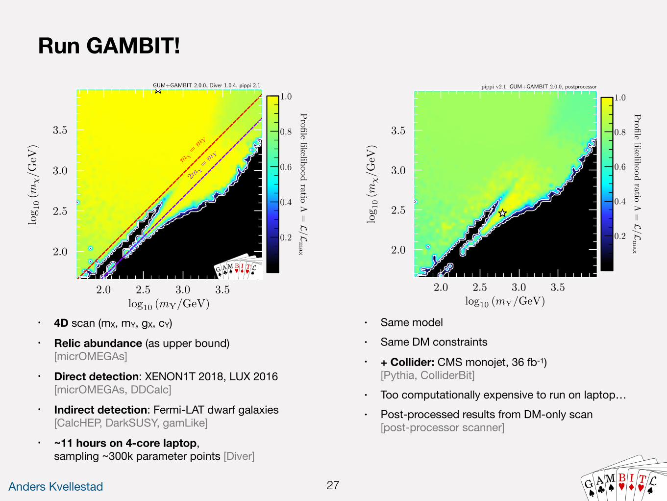
Anders Kvellestad 27 G AM B I T
21
convthresh: 1e-3verbosity: 1
To perform the scan we copy the GAMBIT input fileto the yaml_files folder within the GAMBIT root direc-tory. This is a necessary step, as we need to !importthe appropriate Standard Model YAML file from therelative path include (i.e. the folder yaml_files/includein the GAMBIT root directory). From the GAMBIT rootdirectory, we
cp gum/Tutorial/MDMSM_Tute.yaml yaml_files/
and run GAMBIT with n processes,
mpirun -n n gambit -f yaml_files/MDMSM_Tute.yaml
The above scan should converge in a reasonable timeon a modern personal computer; this took 11 hr to runacross 4 cores on a laptop with an i5-6200U CPU @2.30GHz, sampling 292k points in total. The results ofthis scan are shown below.
Note that whilst the scan has converged statistically,the convergence criterion that we set in the input fileabove is not particularly stringent, so many of the con-tours presented in this section are not sampled wellenough to be clearly defined. A serious production scanwould typically be run for longer, and more e�ort madeto map the likelihood contours more finely. Nonetheless,the samples generated are more than su�cient to extractmeaningful physics.
Once the scan has finished, we can plot the resultusing pippi [84]. As Diver aims to finds the maximumlikelihood point, we will perform a profile likelihoodanalysis with pippi. Assuming that pippi is in $PATH, do
cd gum/Tutorialpippi MDMSM.pip
which will produce plots of the four model parametersagainst one another, as well against as a raft of observ-ables such as the relic abundance and spin-independentcross-section (rescaled by f).
4.4 Results
The upper panel of Fig. 1 shows the profile likelihoodin the plane of the DM mass m‰ against the media-tor mass mY . The relic density requirement maps outthe structure in the same plane. There are two setsof solutions: firstly when the DM is heavier than themediator, m‰ > mY (bordered by the red dashed linein Fig. 1), and secondly where DM annihilates on reso-nance, 2m‰ ¥ mY (centred on the purple dashed linein Fig. 1).
★GUM+GAMBIT 2.0.0, Diver 1.0.4, pippi 2.1
G AM B I T
m �=m Y
2m �
=m Y
2.0
2.5
3.0
3.5
log10(m
�/G
eV)
Profile
likelih
oodratio
⇤=
L/L
max
2.0 2.5 3.0 3.5log10 (mY/GeV)
0.2
0.4
0.6
0.8
1.0
Fig. 1: Profile likelihood in the m‰–mY plane with the relicdensity as an upper bound (upper panel) and as an observation(lower panel). Above the red dashed line at m‰ = mY , DM canannihilate into Y bosons. The purple dashed line at 2m‰ = mY
indicates the region where DM can annihilate on resonance.Contour lines show the 1 and 2‡ confidence regions. The whitestar shows the best-fit point. The grey contours in the lowerpanel the 1 and 2‡ contours from the upper panel.
When m‰ < mY and the Y Y annihilation channel isnot kinematically accessible, annihilation predominantlyoccurs via an s-channel Y to bb or tt, depending on theDM mass. In this case, the only way to e�ciently depleteDM in the early Universe is when annihilation is onresonance, m‰ ¥ mY /2. Away from the resonance whenthe Y Y channel is closed, even couplings of 4fi are notlarge enough to produce a su�ciently high annihilationcross-section to deplete the thermal population of ‰ tobelow the observed value.
When kinematically allowed, ‰‰ æ Y æ tt is thedominant process responsible for depleting the DM
30
★
pippi v2.1, GUM+GAMBIT 2.0.0, postprocessor
�3
�2
�1
0
1
log10g �
Profile
likelih
oodratio
⇤=
L/L
max
�3 �2 �1 0 1
log10 cY
0.2
0.4
0.6
0.8
1.0
★
pippi v2.1, GUM+GAMBIT 2.0.0, postprocessor
2.0
2.5
3.0
3.5
log10(m
�/G
eV)
Profile
likelih
oodratio
⇤=
L/L
max
2.0 2.5 3.0 3.5log10 (mY/GeV)
0.2
0.4
0.6
0.8
1.0
Fig. 8: Combined DM and collider profile likelihood in thecY –g‰ (top) and mY –m‰ (bottom) planes. Excluded regionsmatch that of Figure 1. Contour lines show 1 and 2 ‡ confidenceregions, and the white star the best-fit point.
B.2: SARAH-SPheno
SPheno is a spectrum generator capable of providingone-loop mass spectra as well as decays at tree and looplevel. GAMBIT has included a frontend interface to therelease version of SPheno 3.3.8 since GAMBIT 1.0, andto 4.0.3 since GAMBIT 1.5. Details about the interfacecan be found in Appendix B of [8]. There are importantdi�erences between the frontend interfaces to the releaseversion of SPheno and to the SARAH-generated version(which we refer to as SARAH-SPheno). We give detailsof these di�erences below.
SARAH generates the Fortran SPheno files to com-pute the spectrum and decays for a given model. Thesenaturally di�er from the out-of-the-box SPheno, whichonly works with various versions of the MSSM. After
generating these files with SARAH, GUM moves them tothe main GAMBIT directory, to be combined with thedownloaded version when SARAH-SPheno is built.
In order to improve the usability of SARAH-SPhenoin GAMBIT, we have patched two variables into theFortran code. The first, ErrorHandler_cptr, is a pointerto a void function that returns control to GAMBIT aftera call to the SPheno subroutine TerminateProgram. Thisprevents GAMBIT being terminated when SPheno fails.Instead, it raises an invalid_point exception, and carrieson. The second new variable is SilenceOutput, whichprovides a GAMBIT input option that allows the userto silence all output of SARAH-SPheno to stdout. Thisoption defaults to false.Rules:
- capability: unimproved_new_model_spectrumfunction: get_new_model_spectrum_SPhenooptions:
SilenceOutput: true #default: false
The interface to the spectrum computation fromSARAH-SPheno remains fairly similar to that describedfor the release version of SPheno in Ref. [8]. Some vari-ables and functions have changed names and library sym-bols. The computations have been re-ordered slightly,but otherwise remain unperturbed.
The major change to the spectrum is the additionof mass uncertainties. These are provided to GAMBITupon request using the option GetMassUncertainty. Thisoption defaults to false.Rules:
- capability: unimproved_new_model_spectrumfunction: get_new_model_spectrum_SPhenooptions:
GetMassUncertainty: true #default: false
Setting GetMassUncertainty:true causes the mass uncer-tainties to be added to the spectrum in the SLHA blockDMASS.
The most significant di�erence between the fron-tend interface to SARAH-SPheno compared to therelease version of SPheno is that the former in-cludes computation of decays. The backend conveniencefunction run_SPheno_decays provides a new capabilitySARAHSPheno_new_model_decays, which maps the decaywidths computed by SPheno into a GAMBIT DecayTable.Internally, this backend function fills the SARAH-SPhenointernal variables with the spectrum details and com-putes all the branching fractions using the SARAH-SPheno function CalculateBR. Note that the branchingfractions for charged processes are rescaled within thefrontend interface, as they are double-counted in SPhenoso must be rescaled by a factor of 1/2. Various GAM-BIT input options are added for the computation of thedecays, the most notable of which are
Run GAMBIT!
• 4D scan (mX, mY, gX, cY)• Relic abundance (as upper bound)
[micrOMEGAs]• Direct detection: XENON1T 2018, LUX 2016
[micrOMEGAs, DDCalc]• Indirect detection: Fermi-LAT dwarf galaxies
[CalcHEP, DarkSUSY, gamLike]• ~11 hours on 4-core laptop,
sampling ~300k parameter points [Diver]
• Same model • Same DM constraints • + Collider: CMS monojet, 36 fb-1)
[Pythia, ColliderBit]• Too computationally expensive to run on laptop…• Post-processed results from DM-only scan
[post-processor scanner]
Anders Kvellestad 28
• Global fits are great. We should do more of those.
• The core GAMBIT framework is model-independent
• …but so far it’s taken a lot of work to set up GAMBIT + backends for new theories
• Coming soon: GAMBIT 2.0 w/ GUM
• Auto-generation of GAMBIT code + interfaces for calculations of mass spectrum, decays, dark matter observables, collider physics and vacuum stability
• gambit.hepforge.org
• zenodo.org/communities/gambit-official
G AM B I T
Summary
Anders Kvellestad 29 G AM B I T