the amiba hexapod telescope mount
TRANSCRIPT
arX
iv:0
902.
2335
v1 [
astr
o-ph
.CO
] 1
3 Fe
b 20
09
The AMiBA Hexapod Telescope Mount
Patrick M. Koch1, Michael Kesteven2, Hiroaki Nishioka1, Homin Jiang1, Kai-Yang Lin1,3,
Keiichi Umetsu1,4, Yau-De Huang1, Philippe Raffin1, Ke-Jung Chen1, Fabiola
Ibanez-Romano1, Guillaume Chereau1, Chih-Wei Locutus Huang3,4, Ming-Tang Chen1,
Paul T. P. Ho1,5, Konrad Pausch6, Klaus Willmeroth6, Pablo Altamirano1, Chia-Hao
Chang1, Shu-Hao Chang1, Su-Wei Chang1, Chih-Chiang Han1, Derek Kubo1, Chao-Te Li1,
Yu-Wei Liao3,4, Guo-Chin Liu1,7, Pierre Martin-Cocher1, Peter Oshiro1, Fu-Cheng Wang3,4,
Ta-Shun Wei1, Jiun-Huei Proty Wu3,4, Mark Birkinshaw8, Tzihong Chiueh3, Katy
Lancaster8, Kwok Yung Lo9, Robert N.Martin10, Sandor M. Molnar1, Ferdinand Patt11 &
Bob Romeo10
ABSTRACT
AMiBA is the largest hexapod astronomical telescope in current operation.
We present a description of this novel hexapod mount with its main mechanical
components — the support cone, universal joints, jack screws, and platform
— and outline the control system with the pointing model and the operating
modes that are supported. The AMiBA hexapod mount performance is verified
based on optical pointing tests and platform photogrammetry measurements.
The photogrammetry results show that the deformations in the inner part of
1Academia Sinica, Institute of Astronomy and Astrophysics, P.O.Box 23-141, Taipei 10617, Taiwan
2Australia Telescope National Facility, P.O.Box 76, Epping NSW 1710, Australia
3Department of Physics, Institute of Astrophysics, & Center for Theoretical Sciences, National Taiwan
University, Taipei 10617, Taiwan
4Leung center for Cosmology and Particle Astrophysics, National Taiwan University, Taipei 10617, Taiwan
5Harvard-Smithsonian Center for Astrophysics, 60 Garden Street, Cambridge, MA 02138, USA
6Vertex Antennentechnik GmbH, Duisburg, Germany
7Department of Physics, Tamkang University, 251-37 Tamsui, Taipei County, Taiwan
8Department of Physics, University of Bristol, Tyndall Ave, Bristol, BS8 1TL, UK
9National Radio Astronomy Observatory, 520 Edgemont Road, Charlottesville, VA 22903, USA
10CMA, 1638 S.Research Loop #100, Tucson, AZ 85710, USA
11ESO Headquarters Garching, Germany
– 2 –
the platform are less than 120µm rms. This is negligible for optical pointing
corrections, radio alignment and radio phase errors for the currently operational
7-element compact configuration. The optical pointing error in azimuth and
elevation is successively reduced by a series of corrections to about 0.4′ rms which
meets our goal for the 7-element target specifications.
Subject headings: instrumentation: interferometers
1. Introduction
The Array for Microwave Background Anisotropy (AMiBA) is a dual-channel 86-102
GHz interferometer array of up to 19 elements with a resolution up to 2′. The AMiBA —
located at the Mauna Loa weather station at an elevation of 3.400 m on Big Island, Hawaii
— targets specifically the distribution of high redshift clusters of galaxies via the Sunyaev-
Zel’dovich Effect, (e.g. Sunyaev and Zel’dovich (1972); Birkinshaw (1999) and references
therein), and the anisotropies in the Cosmic Microwave Background (CMB), (e.g. Peacock
(1999)).
In the initial AMiBA operational phase seven close-packed 0.6m diameter Cassegrain
antennas are co-mounted on a fully steerable platform controlled by a hexapod mount. The
typical system noise temperature is ∼ 100 K. From our observations we estimate a sen-
sitivity of ∼ 60 mJy in 1 hour. Previous progress reports were given in Li et al. (2006)
and Raffin et al. (2006). The project as a whole, the correlator and the receivers are de-
scribed elsewhere (Ho et al. 2008; Chen et al. 2008). Observing strategy, calibration scheme
and data analysis with quality checks are described in Lin et al. (2008); Wu et al. (2008);
Nishioka et al. (2008). First AMiBA science results are presented in Huang et al. (2008a);
Koch et al. (2008b); Liu et al. (2008); Umetsu et al. (2008); Wu et al. (2008).
In this paper, we describe the AMiBA mount, which is the largest operating astronomical
hexapod mount. The role of this paper is to provide additional instrumentation details about
this novel hexapod, which complements the science papers. Section 2 introduces the hexapod
mount, with more technical details about its components in appendix A. Section 3 gives an
overview of the pointing corrections and the control system. The explicit pointing model
is presented in appendix B. Photogrammetry measurements and detailed optical pointing
tests verify the mount performance, section 4. Our conclusions are given in section 5.
– 3 –
2. Hexapod Telescope
The design of the AMiBA mount was driven by the requirement of having a lightweight
structure which can easily and quickly be dismantled and shipped to another site for a
possible later relocation and the need of having direct access to the receivers on the platform
for maintenance. The targeted science defined the operating frequency (86-102 GHz), and
hence the required range of baselines, leading to a 6m platform. Array configurations with
maximum baselines require a pointing accuracy of ∼ 0.2′ . Based on these considerations a
hexapod mount with a CFRP (carbon fiber reinforced plastic) platform was chosen.
Whereas the concept of the hexapod (also called Stewart platform, Gough (1956);
Stewart (1965)) is successfully used in many technical applications like machine tools, flight
simulations or complex orthopedic surgery, its application in astronomy has so far been
mostly limited to secondary mirrors for classical Cassegrain telescopes, where the hexapod
is used for focus optimization or wobbling movements to cancel the atmosphere and receiver
noise. A pioneering design of a 1.5m hexapod telescope for optical astronomy was presented
in Chini (2000). Besides this, the AMiBA is the only operating hexapod telescope. The six
independently actuated legs give the Stewart platform six degrees of freedom (x,y,z, pitch,
roll and yaw), where the lengths of the legs are changed to orient and position the plat-
form. This parallel kinematics system has advantages and disadvantages compared to a
serial kinematics system. There is no accumulation of position errors and a generally lower
inertia allows for faster accelerations and slewing velocities. The lower mass, however brings
some risk for oscillations. The control system for the six legs is more complex, because of
more degrees of freedom in motions which can compete and interfere with each other.
For astronomical applications the hexapod offers some interesting possibilities: no el-
evation counterweights and no azimuth bearing are needed and there is no zenith keyhole
compared to a conventional mount. Access to the receivers and correlator from beneath the
platform is straightforward. The sky field rotation (see appendix C) can be compensated,
and polarization measurements are possible by rotating the entire platform.
The AMiBA hexapod with its local control system was designed and fabricated by Vertex
Antennentechnik GmbH, Duisburg, Germany. After a factory acceptance test in 2004 in
Germany, the whole telescope was dismantled, shipped to Hilo, Hawaii and assembled again
on the Mauna Loa site with a final on-site acceptance test in October 2005.
The key components in the Vertex design are: the upper and lower universal joints
(u-joints) with jack screws, which require high stiffness and large travel ranges; the stiffness
of the support cone, to minimize pointing errors from the cone; and the pointing error model
required to meet the 0′.2 pointing requirement.
– 4 –
The AMiBA hexapod has a lower limit of 30◦ in elevation. Azimuth movement is
unlimited without interruption. The hexapod platform polarization (hexpol) range is limited
to ±30◦, with the polarization rotation defined around the pointing axis at any possible
mount position. Both limits are chosen for safety reasons based on structural concerns.
Mechanical hard limit switches are in place to prevent movement beyond these limits in case
of software failure and overriding. The maximum slewing speed is 0.67◦/s. The telescope is
designed to meet the harsh environmental conditions on Mauna Loa, allowing us to operate
with wind speeds of up to 30 m/s (for survival in stow position, wind speeds of up to 65 m/s
can be tolerated) and an operating temperature range of −10◦C to 30◦C (in stow position:
−30◦C to 30◦C). Earthquake survival conditions are met with 0.3 g for both horizontal and
vertical accelerations. The total weight of the mount is ∼ 31,800 kg. (support cone ∼ 16,600
kg, jack screws ∼ 6,000 kg, universal joints ∼ 9,200 kg.) The platform with the interface
ring adds another ∼ 3,000 kg. The current load for the 7 element system is ∼ 500 kg. The
hexapod mount system, schematically illustrated in Figure 14, mainly consists of a support
cone, 6 identical jack screw assemblies with gearboxes, drives and measuring systems, 12
u-joints in total and a CFRP platform. More technical details about these components are
given in appendix A. Observations are started with extended jacks from a neutral position,
Figure 1 Right Panel. The free access to receivers and correlator is shown in Figure 2.
3. Correction Scheme and Control System: an Overview
The hexapod topology is optimized with respect to minimized travel ranges of the u-
joints and to minimized jack screw loads. Since the hexapod position is entirely determined
by the variable length of the 6 jack screws together with the positions of the 6 lower fixed
u-joints, utmost care needs to be taken to accurately monitor the jack screw lengths. The
positions of the 6 lower fixed u-joints have been measured with a laser ranging system
in the Vertex factory in Germany. The first group of pointing corrections on jack level
consist of 4 compensations: jack screw pitch error, temperature compensation, jack screw
rotation error and support cone correction. They all directly yield a length correction for
each individual jack at any given mount position. These error compensations have been
tested and calibrated in the Vertex factory, and the correction algorithms are integrated into
the hexapod control system. Besides the group of jack screw corrections, a second group
of telescope pointing corrections is implemented: radio and optical refraction, an optical
telescope (OT) collimation error correction and an interpolation table (IT) for residual errors.
Only the latter two ones need to be measured, updated and handled by the operator. This
second group leads to corrections in azimuth and elevation, which are then translated into
jack corrections. A detailed description of the pointing error model is in appendix B.
– 5 –
For radio observations the OT collimation error correction is deactivated in the pointing
error model. This assumes that the offsets derived from the optical pointing (with OT
collimation correction, optical refraction and all other corrections activated) are identical to
the errors for the radio pointing (no collimation error correction, radio refraction and all
other corrections activated). In fact, the resolution and the collecting total power of the
0.6m diameter antennas are not sufficient to do a separate radio pointing. However, we use
the correlated signal to verify the relative radio alignment between individual antennas.
We remark that we do not derive explicit corrections for the platform polarization
because the polarization stability and precision have been found to be around 0.1◦ or better
which is good enough for our purposes. We, however, derive azimuth and elevation pointing
corrections for various platform polarizations (section 4.2.2).
The main drive control and the jack length calculations for a commanded position
are done by the ACU (Antenna Control Unit). This also includes the inverse backward
transformation giving the telescope position based on a set of jack lengths. This is essential
for the continuous check between requested and actual telescope position, which is done
in a closed loop system every 5ms and updated depending on the operation. The above
mentioned pointing corrections are calculated on the PTC (Pointing Computer) where they
can be individually activated and displayed. From here they are transferred to the ACU,
illustrated in the flow chart in Figure 3.
The block diagram in Figure 4 summarizes the control system. The actual position,
defined as the real position after applying all the pointing corrections, is displayed on ACU
and reported to the remote TCS (Telescope Control System). A redundant independent
safety level is provided by the HPC (Hexapod Computer) with its PLC (Programmable Logic
Controller). The HPC calculates the telescope position from the jack positions as measured
by the safety (auxiliary) encoders. The PLC is responsible for safety interlocks from limit
switches. Time synchronization is derived from a stratum-1 GPS server, connected to the
ACU with an IRIG-B time signal. Communication between individual computers is through
standard LAN ethernet cables with TCP/IP protocol and NTP for time synchronization,
and it is RS232 and/or CANbus where analog components are involved.
The telescope main operating modes include: Preset, Startrack and Progtrack, with
the latter only possible in remote mode from TCS. Preset moves the telescope to a de-
fined position in (Az,El, hexpol) on a geodesic path, ensuring a short and fast connec-
tion between subsequent mount positions. Startrack tracks a celestial object with either
hexpol=constant or skypol=constant. Progtrack drives the telescope on a defined trajec-
tory in (Az,El, hexpol, time) with a spline interpolation and a maximum stack of 2000 data
points. This mode is extensively used for various types of observation and system checks.
– 6 –
4. Performance Verification
In the initial AMiBA operational phase seven close-packed 0.6m diameter Cassegrain
antennas (Koch et al. 2006) are used on baselines separated by 0.6m, 1.04m and 1.2m. The
antenna field of view (FWHP ∼ 23′) and the synthesized beam (∼ 6′) of the array in
this configuration (at the observing frequency band 86-102 GHz) set the specifications on
the platform deformation and the pointing and tracking accuracy, which are: ∼ 0.6′ rms
pointing error and a platform z-direction deformation of less than 0.3mm.
4.1. Platform photogrammetry
Prior to the integration of the platform and the hexapod in Germany for the factory
acceptance test, we performed stiffness measurements of the CFRP platform on the ground
under expected loading conditions. These measurements were repeated at the Mauna Loa
site. Both measurements showed that the deformations were larger than expected and pre-
dicted by FEA (Finite Element Analysis), especially towards the outer edge of the platform,
even after reinforcement was added. The cause is the segmented structure of the platform,
coupled with inaccurate modeling of stiffness across the segment joints. It was decided to
use the photogrammetry method to verify the platform deformations in a real 7-element
compact configuration on the hexapod.
The first photogrammetry campaign took place during the fall of 2005, with dummy
weights to replace receivers and electronic boxes. In October 2006, we repeated the pho-
togrammetry measurements, this time on the operational 7-element telescope. The results
of the second survey are consistent with the 2005 results. In 2006, we achieved a better
measuring accuracy: about 30µm rms in z (defined as normal to the platform), with a short
term (1-2 days) and a long term (1 week) repeatability better than 80µm rms. We used a
Geodetic Services, Inc. (GSI of Melbourne, Florida) INCA2 single digital photogrammetric
camera. The pictures were processed with a GSI V-STARS 3D industrial measuring system.
About 500 retro-reflective, self-adhesive targets (12mm diameter, ∼ 0.1mm thick) were dis-
tributed over the entire platform surface with a higher target density around receivers. 50
platform positions over the entire azimuth, elevation and platform polarization range were
surveyed.
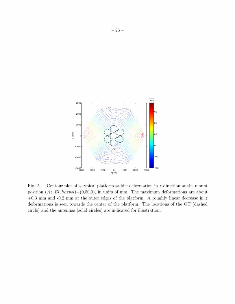
The analysis of the photogrammetry measurements (Raffin et al. 2006; Huang et al.
2008b) reveals a saddle-shaped platform deformation pattern at all surveyed positions, il-
lustrated in Figure 5. The amplitude and phase of this saddle are functions of azimuth,
elevation and polarization. The specifications are met for the 7 antennas in the compact
– 7 –
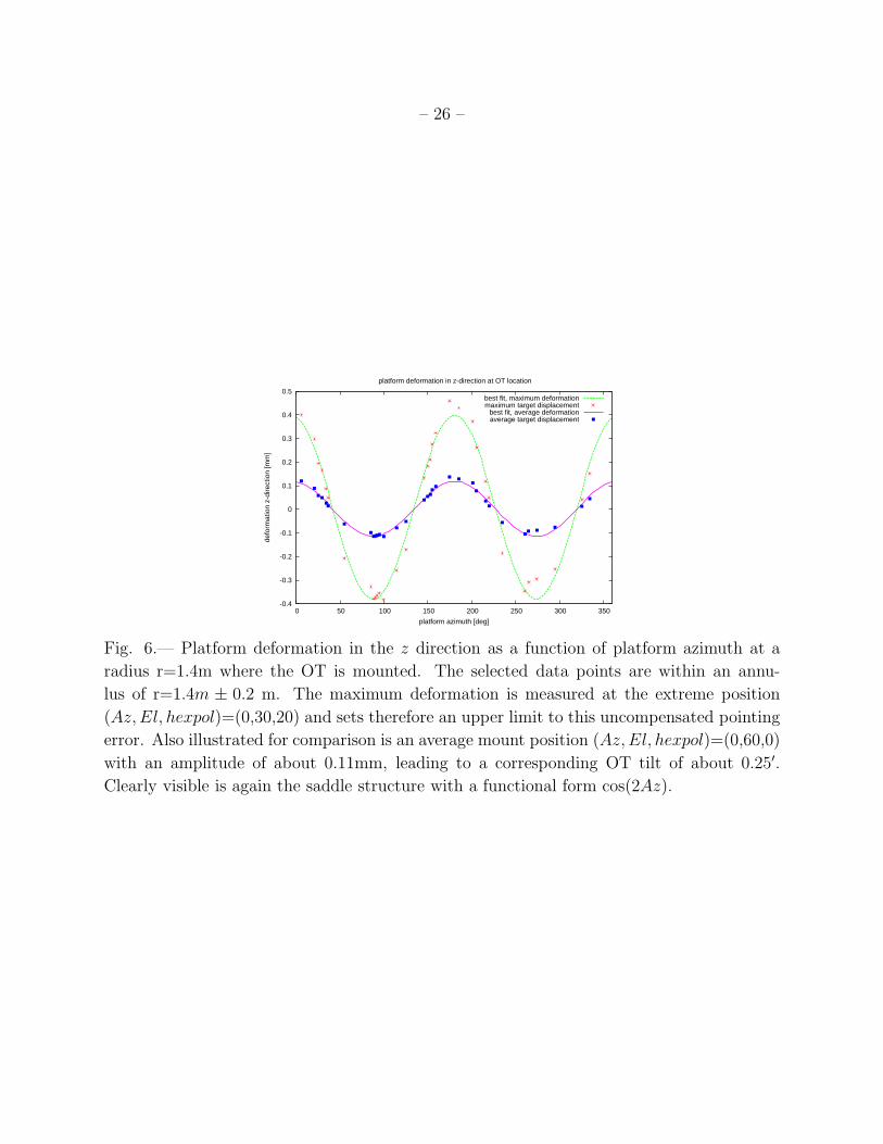
configuration, with a z-deformation amplitude up to 0.120 mm in the inner part of the plat-
form. At the location of the optical telescope (OT), the maximum amplitude (measured
at 30◦ elevation and 20◦ polarization) is about 0.38mm (Figure 6), which leads to an OT
tilt movement with respect to the normal pointing axis of the mount of about ±1′ in this
extreme position. A more average position (Az,El, hexpol)=(0,60,0) is also illustrated for
comparison, showing an amplitude of about 0.11mm, which leads to a corresponding OT tilt
of about 0.25′. As argued in section 4.2, this uncompensated pointing error is acceptable for
the 7-element compact configuration, but will need to be corrected for the planned expansion
phase with 13 elements.
A detailed analysis and model of the saddle type deformation for a 13-element radio
phase correction and an error separation between deformation and pointing error is pre-
sented in Koch et al. (2008a). For this refined analysis we installed a second OT on the
platform. By simply taking the difference between the two data sets of the two OTs, a char-
acteristic signature appears which can be clearly attributed to the platform deformation.
Using a saddle type model as an input for the deformation, the mount pointing error can
be successfully separated. Similarly, with the help of an interpolation scheme based on the
entire photogrammetry data set, the radio phase error from the platform deformation can
be reduced from a maximum 800 µm rms over the entire platform to 100µm or less. The
synthesized beam area is then maintained to within 10% of its non-deforming ideal value.
In this way, the specifications are also met for the 13-element expansion.
4.2. Hexapod optical pointing
Pointing with a hexapod telescope is different from a conventional telescope where a 7- or
13-parameter pointing error model is often used. An important consequence of the hexapod
mount is the absence of azimuth and elevation encoders as compared to more traditional
telescopes. The 3-dimensional locations of the upper and lower u-joints in the measured
reference positions and the jack lengths in any position completely define the geometry of
the mount. The pointing error model therefore needs to take utmost care in treating the
jack lengths and the lower u-joint positions. The 6 upper u-joint locations define a best-fit
plane with its normal defining the resulting pointing axis.
Optical pointing is carried out with a Celestron C8 telescope, equipped with a Fastar
f/1.95 adapter lens and a SBIG ST-237 CCD camera. The resulting field of view (FoV) is
about 30′ × 20′ on a 652 × 495 pixel array, giving a calibrated pixel scale of about 3.81′′. A
preliminary rough OT collimation error is measured on the platform with a digital tiltmeter
and compensated in the pointing error model, following equation (B8) and (B9).
– 8 –
4.2.1. Pointing with hexpol=0
In order to achieve the required pointing accuracy of 0.6′ or better, a two-step approach
is adopted. In a first pointing run all the known pointing corrections (section 3) except the
interpolation table (IT) are activated on the pointing computer (PTC). As a function of
the mount position, (Az,El, hexpol = 0), the offsets (∆xk, ∆yk) of a target star k, with
respect to the center of the CCD image, are split into an Az and El error in a common
reference frame at Az = 0. This involves rotating the CCD images by the mount Az (and
hexpol) coordinate, together with an additional rotation γ for the orientation of the CCD
with respect to the sky. This yields the CCD frame - mount frame transformation (Figure
7): (∆Azraw,k
∆Elraw,k
)=
(cos βk sin βk
− sin βk cosβk
)(∆xk
∆yk
), (1)
where βk = Azk + hexpolk + γ for each star image k at the mount position k. The raw
errors (∆Azraw,k,∆Elraw,k) are then analyzed to separate the remaining uncompensated
OT collimation error from the real mount pointing error. (∆Azcoll,OT ,∆Elcoll,OT ) has a
characteristic azimuth and elevation signature of the form:
(∆Azcoll,OT
∆Elcoll,OT
)=
(CAz
CEl
)+ A
(cos(Az + φ)
cos(Az + φ+ π/2)
), (2)
where A and φ are the OT uncompensated tilt amplitude and phase, respectively, which
reflect the remaining OT collimation error and (CAz, CEl) are two constants. Assuming a
rigid OT, the amplitude A is identical for the azimuth and elevation signature and their
phases are separated by π/2. The small fitting residuals ∆AzIT , ∆ElIT (of the order of 1′
or less) populate the IT, which is a three-dimensional table in Az, El and hexpol:
(∆AzIT,k
∆ElIT,k
)= (3)
(∆Azraw,k
∆Elraw,k
)−
(∆Azcoll,OT
∆Elcoll,OT
)+
(CAz
CEl
).
The irregular grid errors (∆AzIT,k,∆ElIT,k) are then transformed into a regular spaced
grid with the cubic Shepard algorithm (Renka 1999), finally generating the IT pointing
corrections (∆AzIT ,∆ElIT ).
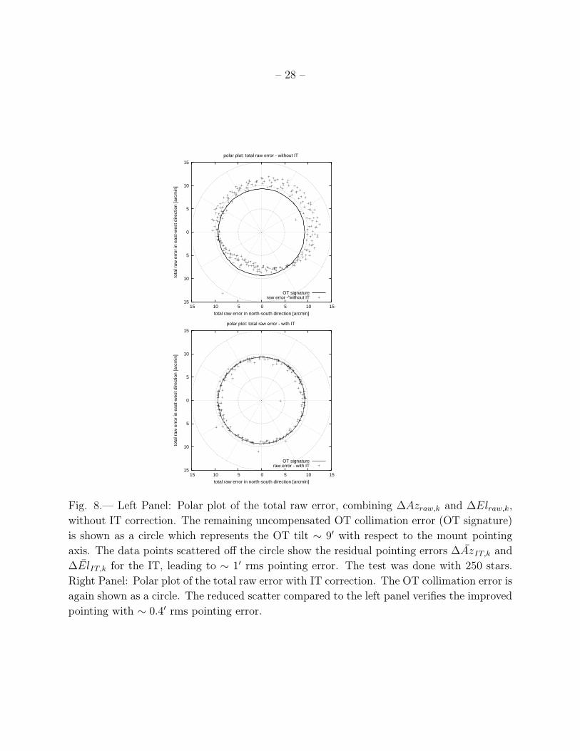
In a second pointing run all the known pointing corrections and the IT are activated
on the PTC. This verifies that the mount errors are reduced with the IT and that only
the OT collimation error remains. These small errors are checked every few weeks for their
– 9 –
repeatability. Typically, one IT iteration is needed to reduce an initial pointing error in
Az and El from ∼ 1′ rms to about ∼ 0.4′ rms. Subsequent pointing tests have revealed
almost exactly the same numbers (within repeatability, section 4.3), so that our IT has
been unchanged over the year of data-taking. The iterative improvement with the IT is
illustrated in Figure 8, where the total raw error,√
∆Az2raw,k + ∆El2raw,k, is shown in a
polar plot over the entire azimuth range. In this strategy it is crucial to identify properly
the remaining uncompensated OT collimation error (∆Azcoll,OT ,∆Elcoll,OT ) to make sure
that the small remaining values in the interpolation table compensate only and exclusively
for the hexapod mount errors. For radio observations the OT collimation error correction
is deactivated in the pointing error model. This assumes that the pointing errors derived
from the optical pointing (with OT collimation correction, optical refraction and all other
corrections activated) are identical to the errors for the radio pointing (no collimation error
correction, radio refraction and all other corrections activated). No separate radio pointing
is done because the 0.6m antennas (FWHM ∼ 23′) do not have enough gain to allow us to
verify the required pointing accuracy. In order to have the most rigid measure, the OT is
installed close to one of the upper u-joint positions. Possible local irregularities and position-
dependent platform deformations which can affect the rigidity of the OT need to be filtered
out if the pointing needs to be further improved (Koch et al. 2008a).
The interpolation table approach further assumes that the remaining mount errors are
sufficiently smooth enough functions in between neighboring pointings, leading to the ques-
tion of the optimized pointing cell size. We find that 100 stars, approximately evenly dis-
tributed in solid angle over the entire accessible sky, resolve the pointing features reasonably
well. Observing more stars does not significantly improve the pointing. Typically, we need
about 1 hour to observe 100 stars in a fully automatic mode, where the telescope is driven
from high to low elevation on a spiraling trajectory1 . A multiple of this time is required if
different platform polarizations for each star are included.
Although not necessary in the interpolation table approach, we found it useful to further
analyze the residuals and identify their origins. A more detailed fitting including the mount
1 In the initial phase, the mount and pointing performance were extensively tested by driving the telescope
manually from a few randomly chosen initial positions to the same target position. These tests indeed helped
to identify flaws in the control software. Subsequently, with the stable control algorithm, different trajectories
were found to be equivalent. For the automatic mode a spiraling trajectory was then adopted because this
leads to the most efficient sky coverage with a minimized overhead in telescope drive time.
– 10 –
tilt:
(∆Azraw,k
∆Elraw,k
)= (4)
(∆Azcoll,OT
∆Elcoll,OT
)+ B
(cos(Az + ψ) × sin(El)
cos(Az + ψ + π/2)
),
where (cos(Az+ψ)× sin(El), cos(Az+ψ+π/2)) is a term taking into account an additional
mount tilt, improved the goodness of the fit only marginally, but still revealed a mount
cone/foundation tilt of ∼ 0.2′ with respect to zenith. Furthermore, our control software
allows us to simulate a small rotation of the entire telescope. In this way we identified a
slight misorientation of the cone with respect to north of ∼ 1′. These effects contribute
partly to the constants (CAz, CEl) in equation (2). Since both errors are small, we simply
absorb them in the IT.
4.2.2. Pointing with hexpol 6=0
Extracting the polarization corrections relies on the proper identification of the OT
signature. This is best done at hexpol = 0, since at hexpol 6= 0 the polarization error and
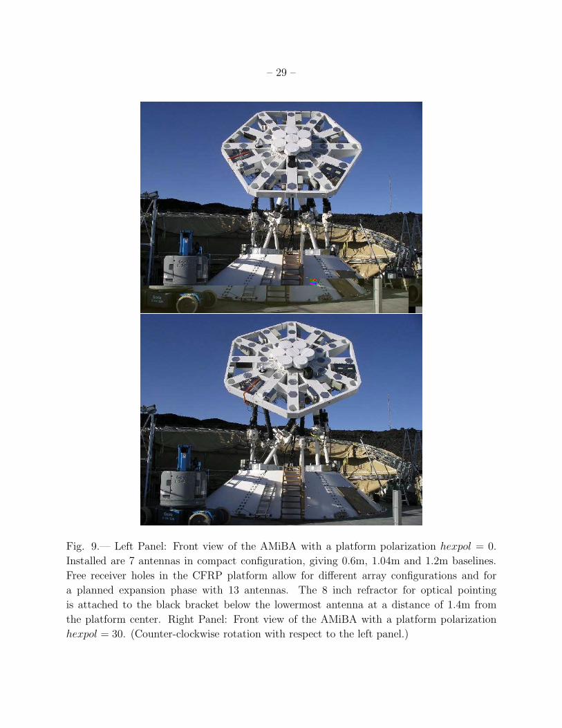
the OT signature become degenerate. The hexpol movement is illustrated in Figure 9. For
the OT itself, the hexpol 6= 0 case is only an additional rotation, identical to an azimuth
position with az + hexpol, as described in equation (1). We are thus extracting the OT
signature at hexpol = 0 assuming it to be rigid enough, so that any position error with a
polarized platform, as a function of (Az,El, hexpol), becomes:
(∆AzIT,k
∆ElIT,k
)= (5)
(∆Azraw,k
∆Elraw,k
)−
(∆Azcoll,OT
∆Elcoll,OT
)
hexpolk
+
(CAz
CEl
),
where (∆Azraw,k,∆Elraw,k) are again defined as in equation (1) with hexpol 6= 0 and
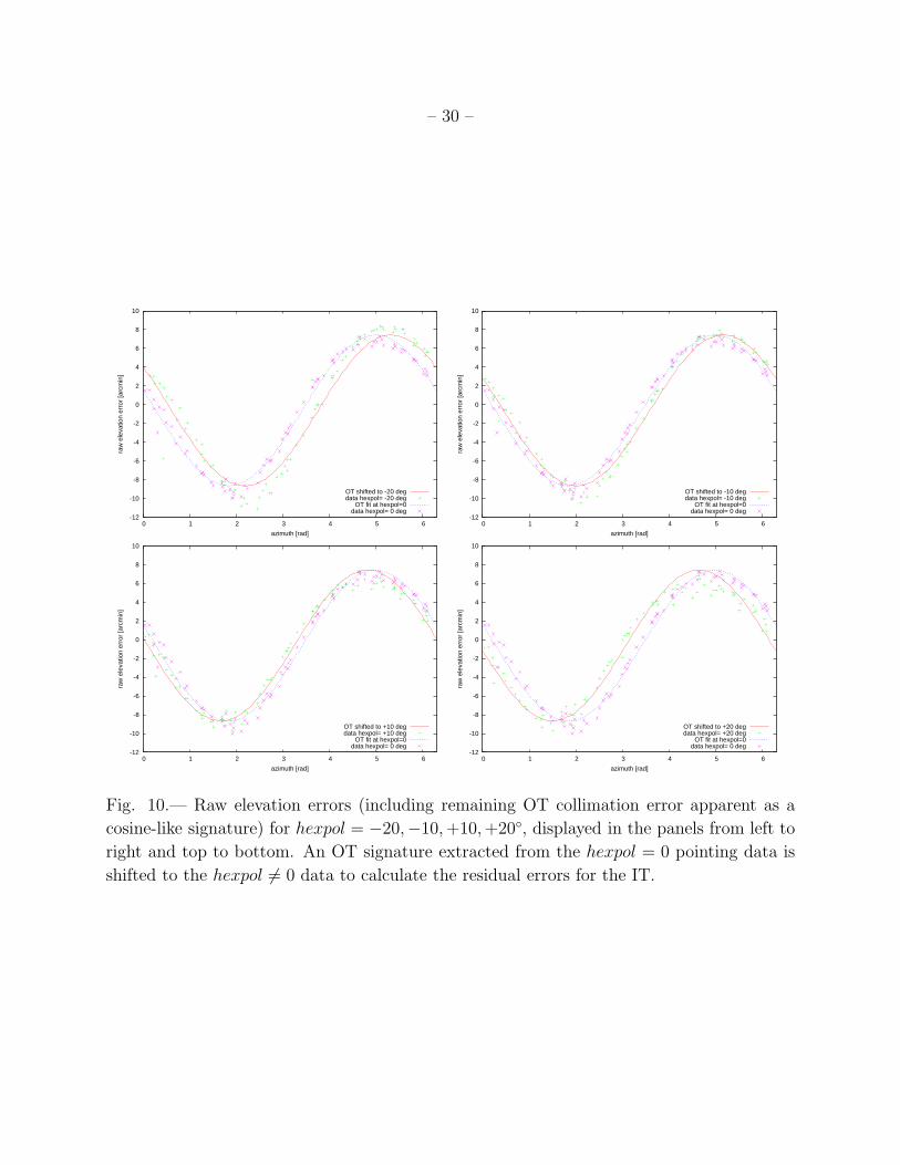
(∆Azcoll,OT ,∆Elcoll,OT )hexpolk are the OT signatures shifted by hexpolk, Azk → Azk+hexpolkin equation(2). This is illustrated in Figure 10 for the raw elevation errors, where polarization
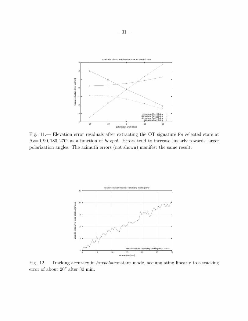
pointing was done with hexpol=±20,±10, 0◦ for 100 stars. Clearly seen is the OT signature
with the hexpol = 0 case shifted to the different hexpol angles. The residual polarization
errors increase linearly with the polarization angle, from ∼ 0.8′ to ∼ 3′ for 0◦ to 20◦, as
shown in Figure 11 for the polarization dependent elevation error. We remark that we do
not explicitly correct for a polarization error. We found that the uncertainty in the polar-
– 11 –
ization angle is within 0.1◦ or better, which is negligible for the later pointing error analysis
and our observations.
We finally consider the influence of the platform deformation (section 4.1) on the point-
ing error analysis. The local saddle-type deformation with a z-direction amplitude of typ-
ically 100µm at the OT radius will slightly change the OT’s phase and amplitude as a
function of the mount position, and therefore introduce a local position dependent error
which is under-/overcompensated in the IT. However, a 100µm amplitude leads to an es-
timated wiggling of the OT of about 0.25′. For the 7-element compact configuration we
consider that acceptable and we therefore have not further extracted this component.
4.3. Repeatability
A key parameter to ensure the reliability of the entire system is the pointing repeata-
bility. Factory tests have revealed short term repeatability errors between 1′′ and 7′′ in Az
and El2 , respectively. Two astronomical tests with the OT were performed: First, in an
overall repeatability test, two runs with 250 stars (distributed on equal solid angles over
the complete accessible celestial sphere) were executed during the same night, the 2nd run
immediately after the 1st one, with almost identical atmospheric conditions. Secondly, in a
star position test, aiming at the day-to-day repeatability, a set of 8 stars in different direc-
tions and elevations was observed on two subsequent days at the same time. CCD images
were then taken by going back and forth between two stars of this set. Some stars could be
observed at almost exactly the same time at almost identical mount positions. Both tests
show consistent results: A cell-to-cell comparison from the overall repeatability test gives an
average Az and El error difference of 5.7′′ and 2.5′′, respectively. The star position tests show
a day-to-day repeatability better than 4′′. From the same test it could also be verified that
small changes in the mount position introduce only small linear deviations in the pointing
and tracking errors.
The long term repeatability has been checked on a roughly weekly basis in the early
mount testing phase. Later, with each additional receiver element integrated into the array,
pointing tests have been routinely carried out. All these results are consistent within the
short term repeatability errors. Over the more than two years operation of the 7-element
compact configuration, a very robust pointing performance was verified, with no measurable
2 For these tests a laser source was installed on the platform. The mount was repeatedly driven to the
same target position after going back to an initial position. The slight shifts in the locations of the projected
laser beams on the factory wall were then used to characterize the repeatability at the target positions.
– 12 –
changes due to temperature or other environmental effects, or additional weight on the
platform.
4.4. Tracking
Tracking tests were performed over short time periods, typically about 30 minutes. This
ensures that tracking results are not or only minimally biased by any uncompensated pointing
errors. 30-minute tests mean that pointing stars remain within a single IT cell. The tracking
tests were done in both polarization modes, hexpol=constant and skypol=constant.3 In the
hexpol=constant mode, a linearly increasing tracking error was measured over 30 minutes,
accumulating to 20′′ after 30 minutes in Figure 12. The skypol=constant mode shows a
field rotation stability of about 3.6′ rms with respect to an initial polarization direction over
30 minutes, Figure 13. Since tracking is internally handled as a fast sequence of pointing
positions, the long-term tracking error (several hours or large ranges in Az, El and hexpol)
is controlled by all the pointing corrections including the IT. On short timescales (within
interpolated errors in the IT) the measured tracking error reflects a combination of par-
tially uncompensated pointing errors and tracking-specific errors4. Our normal observations
(Wu et al. 2008) are carried out in a lead/trail-main field procedure over about 6 minutes.
The tracking error is therefore negligible.
4.5. Array Efficiency
Based on the measured pointing accuracy we quantify the array efficiency. Besides this
absolute mount pointing error (p), which misaligns each antenna by the same amount, we
3hexpol=constant: A celestial object is tracked by keeping the intrinsic platform polarization constant.
In this mode, any possible complication from the additional polarization movement is avoided, making it
a clean measure of tracking performance. In order to separate the tracking and pointing errors, tracking
is done only over a short time (small angular range), where the pointing error is supposed not to change
significantly. Longer tracking tests require the use of the IT.
skypol=constant: A celestial object is tracked by fixing a polarization on the sky, introducing therefore a
counter-rotation of the hexapod to compensate for the sky rotation. This checks the tracking stability of the
mount. Constant skypol mode is essential for polarization measurement and control of baseline orientations.
We test this mode by monitoring the orientation of a vector between two stars.
4 Tracking-specific errors result from the moving telescope, contrary to the pointing errors where the
telescope accuracy is measured at a fixed position. However, on a short time-scale tracking errors are
typically small, and they are therefore not further taken into account in the analysis.
– 13 –
also take into account the measured platform deformation error (d) and a radio misalignment
error (m) for each antenna pair (baseline). d and m define a relative error which measures
the shift in the overlap of two antenna primary beams. Additionally, they can also alter the
absolute pointing error of each antenna, worsening or improving it due to the local pseudo-
random character of the errors. This resultant total pointing error defines the loss in the
synthesized beam product (Koch et al. 2008a). Due to the complicated position dependence
of all these errors, we use a Monte-Carlo simulation (10,000 realizations) to quantify the loss.
We assume uniformly distributed errors: p ∈ [−0.4, 0.4]′, d ∈ [−1, 1]′, m ∈ [−2, 2]′. The error
interval for d is a conservative estimate from the photogrammetry results, m corresponds to
∼ 10% of the antenna FWHP, which is approximately the achievable mechanical alignment
limit. The expected efficiency is about 93%. With p ∈ [−1, 1]′ the efficiency drops to about
90%.
5. Conclusion
The hexapod design has some interesting advantages compared to a conventional mount.
From an engineering point of view, it offers a relatively compact design for transportation
and possible relocation, a simple cable wrap and ease of access to the receivers from beneath
the platform, which is important for daily maintenance and easy reconfiguration of the base-
lines. For its astronomical application, there is no zenith keyhole, polarization movements
are controlled by the same algorithm actuating all six jack lengths and no additional me-
chanical polarization axis is needed as in the case of the CBI telescope (Padin et al. 2000).
Compromises have to be made, leading to a reduced elevation and polarization range of 30◦
and ±30◦, respectively. Whereas the hexapod offers six degrees of freedom, for its traditional
astronomical application only three degrees are used. The AMiBA hexapod is essentially
driven along geodesics on a sphere, both for tracking and slewing. Tracking is approximated
as a sequence of multiple segments of great circles. Direct and even shorter travel ranges for
slewing, following simple translational movements on a straight line, have not been imple-
mented for safety reasons. The hexapod however offers additionally the possibility of small
movements along the pointing directions if this should be of astronomical interest.
Pointing with a hexapod is very different from a conventional mount. Position errors
are not accumulated as in a serial kinematics system, but the control system is significantly
more complex. Utmost care needs to be taken to determine all the jack lengths accurately.
With one IT iteration the current pointing accuracy is ∼ 0.4′ rms in azimuth and elevation,
which meets the requirements for the 7-element array compact configuration baselines. An
uncompensated pointing error from the platform deformation of the order ∼ 0.25′ still keeps
– 14 –
it in an acceptable range, but needs to be further analyzed for the planned expansion phase.
Position errors with polarization movements without IT compensation are typically linearly
increasing with polarization as a result of a slight drift of the platform center during the
rotation, which is a consequence of the absence of any mechanical polarization axis. This is
also compensated with the IT. Laser ranging techniques - along the jack screws or mounted
on the ground to determine the orientation of the platform - might be a possible choice to
further improve the pointing accuracy of a hexapod.
Acknowledgment We thank the anonymous referee for providing useful comments and
suggestions. We thank the Ministry of Education, the National Science Council, and the
Academia Sinica for their support of this project. We thank the Smithsonian Astrophysical
Observatory for hosting the AMiBA project staff at the SMA Hilo Base Facility. We thank
the NOAA for locating the AMiBA project on their site on Mauna Loa. We thank the
Hawaiian people for allowing astronomers to work on their mountains in order to study the
Universe. We thank all the members of the AMiBA team for their hard work. Support from
the STFC for MB and KL is also acknowledged.
A. Hexapod Main Components
A.1. Support Cone
The support cone provides stiffness and inertia for the drive system. It consists of 3
inner and 3 outer truncated cone steel segments. Individual segments are connected with each
other with butt-strap joints for the highest stiffness. Corrosion protection is assured with a
3-layer paint system. The anchoring is leveled to about 0.1◦. Due to environmental and cost
concerns associated with excavation on Mauna Loa, the cone is not embedded but is sitting
on the concrete foundation. A future cone insulation should further improve its thermal
behavior. A finite element analysis (FEA) was done in order to optimize a low structural
weight and minimize the pointing error contribution. Simulated load cases included gravity,
10 m/s side wind, 10 m/s front wind, a temperature gradient along the cone axis with
∆T=1K and a temperature difference between the steel cone and the concrete foundation
with ∆T=2K. In order to separate the pointing error contribution of the support cone from
the rest of the telescope, the entire structure above the cone was modeled to be perfectly
rigid with no reaction forces. The wind loads were treated as resultant nodal point forces
on the platform gravity center. The FEA demonstrated that the contact area between the
support cone and concrete foundation is everywhere under pressure in any operational state.
The main pointing error contribution then comes from the gravity load with maximum errors
– 15 –
at lowest elevation and maximum polarization of about 8′′ and 3′′ in azimuth and elevation,
respectively. Temperature gradients (within the cone and between cone and concrete ground)
contribute in total about 1′′ to azimuth and elevation pointing errors. 10m/s front and side
winds can give up to 1′′ pointing error contribution. Generally, the pointing error in both
azimuth and elevation increases by about 4′′ to 8′′ if the polarization is changed from 0◦ to
30◦. These errors are calibrated with the help of an interpolation table (appendix B).
A.2. Universal Joints and Jack Screws
Very stiff and backlash-free u-joints are necessary in order to meet the pointing re-
quirement, because of the high torques under drive conditions, the large shear forces at
low elevation, and because u-joint deformation cannot be detected directly. Zero backlash
is achieved by tapered roller bearings which are preloaded in the axial direction. A large
angular range of motion (partly up to ± 52◦) in tangential and radial direction is necessary
to achieve the telescope travel range. Minimizing the travel range of the u-joints and jack
screws by keeping small dimensions, low weight and high stiffness has been one of the key
design achievements. The end positions of the u-joints are monitored by limit switches which
shut off the servo system.
The jack screws consist of a tubular ball screw with an integrated low backlash worm
gear with a transmission ratio 10.67:1. Each jack is driven by a motor and a low backlash
bevel gear with transmission ratio 4:1. The ball screw spindle of the jack screw is engaged
in the worm gear by a backlash-free axial preloaded double nut, which is also free from axial
backlash. The jacks, each with a maximum operation load of 100 kN, can be driven at a
stroke rate of 0 to 20 mm/s. An absolute (main) angular encoder5 is mounted at the shaft
of the worm gear for an accurate measurement of the jack screw length. If necessary, this
can be upgraded with a laser interferometer for a direct measurement of the actual jack
screw length, to compensate for errors in the jack screw pitch, the jack elastic deformation
and the jack screw and worm gear backlash. It is estimated that this would improve the
pointing accuracy from ∼ 10′′ to about ∼ 3′′. Since a hexapod design does not allow for
hardware switches to limit the travel range of a telescope, a second set of encoders (auxiliary
encoders) has been included for independent determination of jack and telescope positions
in a separate safety controller, the HPC (Figure 4).
5 The encoder resolution is 13 bit × 4096 revolutions with a ±1 bit accuracy, which leads to a 0.23µm
overall resolution for a jack pitch of 20mm. According to the manufacturer’s specifications, the measurement
inaccuracy is < 0.1µm, which has a negligible influence on the pointing error.
– 16 –
The jack screws have a minimum and maximum length of about 2.8m and 6.2m, re-
spectively, with a maximum travel range of 3.4m. They can be fully retracted to bring the
telescope into a stow position (Figure 1 Left Panel), which allows us to close the shelter
and protect the telescope and instruments from inclement weather and windy conditions.
Observations are started with extended jacks from a neutral position, Figure 1 Right Panel.
A.3. CFRP Platform
The AMiBA platform was designed by ASIAA and fabricated by CMA (Composite
Mirror Applications, Inc.), Tucson, Arizona, USA. In a segmented approach, the central
piece and the 6 outer elements are bolted together. There are 43 antenna docking positions,
allowing for multiple configurations for the array, with baselines from 0.6 to 5.6 m. The
receivers are sited behind the antennas and fit through apertures in the platform. The free
access to receivers and correlator is shown in Figure 2. Cables and helium lines are guided
with a central fixed cable wrap at the back of the platform. An optical telescope for optical
pointing tests has been attached to one of the free receiver cells near the upper u-joints.
Two photogrammetry surveys in 2005 and 2006 (Raffin et al. 2006) have revealed that the
platform deformation during operation is within the specifications of the 7-element compact
configuration (section 4.1).
B. Pointing Error Model
The pointing corrections on jack level consist of 4 compensations6 : jack screw pitch
error, temperature compensation, jack screw rotation error and support cone correction.
A jack pitch error correction is essential since the real length of a jack is not directly
measured. Only the rotation of the worm gear is measured. Each jack has therefore been
calibrated with a correlation function for the exact length against jack screw pitch error
compared to the encoder readout. The repeatable measurements are fitted with a polynomial
of order 10, leading to a pitch error length correction ∆Lp,i for each jack i = 1, ..., 6, coded
in the software:
6Load cells were considered to measure the elastic jack screw deformation due to gravity. Estimates
including a finite element analysis predict a maximum length error due to the bending of about 160 µm only.
The elastic deformation error is therefore not explicitly modeled as a pointing error component, but simply
absorbed in the error interpolation table.
– 17 –
∆Lp,i ∼
10∑
k=1
aik (xi)k , (B1)
where aik are the fitting coefficients and xi is the jack length.
The jack screw length variations due to temperature changes are monitored with 3
temperature sensors along each jack. The resulting change in length ∆LT,i is calculated as:
∆LT,i =
∫ li
0
αfi(x) dx, (B2)
where α = 12.0 × 10⁻⁶K−1 is the linear thermal expansion coefficient for ordinary steel and
li is the position dependent length of the jack i. fi(x) is a linear approximation to the
temperature distribution along the jack i:
fi(x) =
∆T1,i : x ≤ P1,i,∆T2,i−∆T1,i
P2,i−P1,i(P2,i − x) +
∆T1,i P2,i−∆T2,i P1,i
P2,i−P1,i: P1,i < x ≤ P2,i,
∆T3,i−∆T2,i
P3,i−P2.i(P3,i − x) +
∆T2,i P3,i−∆T3i P2,i
P3,i−P2,i: P2,i < x ≤ P3,i,
∆T3,i : x > P3,i,
where P are the positions of the temperature sensors along the jacks. The temperature
changes ∆T are calculated with respect to a reference temperature at 17◦C.
Because of the spindle thread, a jack screw length change can occur which is not detected by
the encoder on the worm gear shaft. Using Euler angles to calculate the kinematics of each
jack screw, this undetected rotation βi can be expressed with respect to a reference angle
βref,i, yielding a rotation error compensation ∆Lr,i of the form:
∆Lr,i = (βref,i − βi)p
2π, (B3)
where p=20 mm/rotation is the jack screw pitch.
A support cone compensation model takes into account the deformation of the cone due
to temperature changes. The slight shift of the lower fixed u-joints is then calculated by
assuming that they expand on concentric circles with a temperature averaged over several
sensors in the cone:
xnew = x+ xα (T − T0), (B4)
ynew = y + y α (T − T0), (B5)
where x and y are measured reference coordinates of the lower u-joints at a reference temper-
ature T0 = 17◦C. α = 12.0× 10⁻⁶K−1 as for the jack screws. When calculating the required
– 18 –
jack lengths from the requested telescope position, this coordinate change results in a slight
change of the required jack lengths.
Besides the group of jack screw corrections, a second group of telescope corrections is
implemented: radio and optical refraction (e.g. Patel (2000)), an optical telescope (OT)
collimation error correction and an interpolation table (IT) for residual errors. The radio
refraction algorithm for the elevation correction ∆Elref,radio in radians is taken from Allen
(1973):
∆Elref,radio = ref0/ tan(El), (B6)
where ref0 = (N2−1)/2N2 with N = 1− (7.8×10⁻⁵×P +0.39×wv/T )/T . T ,P and wv are
the temperature in K, the atmospheric pressure in mbar and the water vapour pressure in
mbar, respectively. The calculation of the water vapour pressure wv is based on the measured
relative humidity H on the site:
wv =H
100Psat,
where the saturation pressure of the water vapour in mbar is Psat = c0 × 10c1×T/(c2+T ) with
the numerical constants c0 = 6.1078, c1 = 7.5, c2 = 237.3 and the temperature in ◦C.
The optical refraction correction in radians used for optical pointing observations is adopted
from Seidelmann (1992) and implemented as:
∆Elref,opt = 1.2 ×P
1013.2
283.15
T×
60.101 tan(dZ) − 0.0668 tan3(dZ)
(180/π)3600(B7)
where dZ , P and T are the distance from the zenith in radians, the atmospheric pressure in
mbar and the ambient temperature in K, respectively.
For both refraction correction modes we use annually-averaged values for the weather
data. Extreme weather variations cause changes in the refraction corrections of the order of
fractions of arcseconds and are therefore negligible for our wavelength and antenna size.
The optical telescope (OT) collimation error is corrected in the form:
∆AzOT =Hx cos(φaz + φpol) +Hy sin(φaz + φpol)
cos(φel)(B8)
∆ElOT = Hy cos(φaz + φpol) −Hx sin(φaz + φpol), (B9)
where Hx and Hy are the two tilt angles of the OT with respect to the mount pointing axes
in the reference plane of the platform. φaz and φpol are the mount azimuth and the platform
polarization, respectively.
A final pointing correction is done with an interpolation table (IT). Small measured
pointing errors which are not explicitly modeled can be entered here. The three-dimensional
– 19 –
table yields corrections ∆AzIT ,∆ElIT as a function of Az, El and hexpol through a linear
interpolation. Typically, we build the table with about 100 entries, the largest discontinuities
of ∼ 50◦ are at the highest elevations around 85◦. Lower elevation with larger errors are
resolved at ∼ 20◦.
For the control system the sums of jack and telescope corrections are then used:
∆Ltot,i = ∆Lp,i + ∆LT,i + ∆Lr,i, (B10)
∆Aztot = ∆AzIT + ∆AzOT , (B11)
∆Eltot = ∆ElIT + ∆ElOT + ∆Elref , (B12)
where ∆Aztot and ∆Eltot again lead to an effective change in jack length which is subject to
pointing corrections. ∆Elref is either the radio or optical refraction correction.
All the pointing corrections are calculated on the PTC (Pointing Computer). From here
they are transferred to the ACU in the form described in equations(B10)-(B12), illustrated
in the flow chart in Figure 3. The ACU applies corrections as:
Lact,i = Lenc,i + ∆Ltot,i, (B13)
where Lenc,i and Lact,i are the encoder measured and the real actual length of jack i, respec-
tively. Equally, the actual position (Azact, Elact), defined as the real position after applying
all the pointing corrections, is displayed on ACU and reported to the remote TCS (Telescope
Control System) as:
Azact = Az + ∆Aztot, (B14)
Elact = El + ∆Eltot, (B15)
where (Az, El) is the telescope position as calculated from the corrected jack lengths Lact,i
in equation(B13). The block diagram for the local control system is shown in Figure 4.
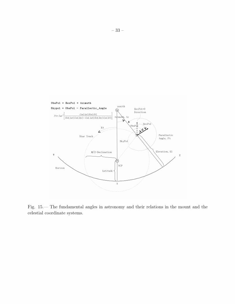
C. hexpol, skypol and the sky coordinates
The interferometer baselines are fixed with respect to the platform. To describe the
platform orientation, we use the mount coordinate system (Az, El, ObsPol), where ObsPol
refers to the angle between a specified axis on the platform and the line joining the zenith
and the current pointing. This specified axis points toward south when the hexapod is in
neutral position. The platform rotation is nominally related to the pointing by the relation
ObsPol = Az. However, the hexapod is capable of changing the rotation by ±30◦ away
from this relation. We define the added rotation as hexpol and rewrite the relation as
– 20 –
ObsPol = Az + hexpol.
The platform orientation can also be written in the sky coordinates (ha, dec, skypol), where
ha and ra are the hour angle and declination, respectively, in the equatorial coordinate
system. skypol thus describes the angle between the specified axis and the line joining
the current pointing and the North Celestial Pole (NCP). The transformation between the
two system depends on the latitude (lat) of the observatory as written below. Figure 15
illustrates the relation between the different angles and the two coordinate systems. The
basic transformation relations, including parallactic angle (PA), are:
sin(El) = sin(lat) sin(dec) + cos(lat) cos(dec) cos(ha),
cos(El) cos(Az) = cos(lat) sin(dec) − sin(lat) cos(dec) cos(ha),
cos(El) sin(Az) = − cos(dec) sin(ha),
skypol = obspol − PA,
PA = tan−1
(cos(lat) sin(ha)
sin(lat) cos(dec) − cos(lat) sin(dec)cos(ha)
).
REFERENCES
Allen, C.W., 1973, in: Astrophysical Quantities, Humanities Press, Inc. 3rd ed.
Birkinshaw, M., 1999, Phys. Rep. 310, 97
Chen, M.-T., et al., 2008, ApJ, in preparation
Chini, R. 2000, Reviews in Modern Astronomy, 13, 257
Gough, V. E., 1956, in Proc. Auto Div. Inst. Mech. Eng., pages 392-394, 1956-1957.
Ho, P.T.P., et al., 2008, ApJ, accepted, arXiv:0810.1871
Huang, C.-W., et al., 2008a, ApJ, in preparation
Huang, Y.-D., et al., 2008b, in Proc.SPIE, Vol.7012, 70122H, Ground-based and Airborne
Telescopes
Koch, P., et al., 2006, in Proc.EuCAP (ESA SP-626), p.668.1
Koch, P., et al., 2008a, in Proc.SPIE, Vol.7018, 70181L, Advanced Optical and Mechanical
Technologies in Telescopes and Instrumentation
Koch, P., et al., 2008b, ApJ, in preparation
– 21 –
Li, C.-T., et al., 2006, in Proc.SPIE, Vol.6275, pp. 487-498, Submillimeter Detectors and
Instrumentation for Astronomy III
Lin, K.-Y., et al., 2008, ApJ, submitted
Liu, G.-C., et al., 2008, ApJ, in preparation
Nishioka, H., et al., 2008, ApJ, accepted
Padin, S., et al., 2002, PASP, 114, 83
Patel, N.A., 2000, in SMA Technical Memo No.139,
http://sma-www.cfa.harvard.edu/memos/
Peacock, J.A., 1999, in: Cosmological Physics, Cambridge University Press
Raffin, P., et al., 2006, in Proc.SPIE, Vol.6273, pp. 468-481, Optomechanical Technologies
for Astronomy
Renka, R.J., 1999, in ACM Transaction on Mathematical Software (TOMS), v.25, n.1,
Seidelmann, P.K., 1992, in: Explanatory Supplement of the Astronomical Almanac, Univer-
sity Science Books, Mill Valley, California
Stewart, D., 1965, in UK Institution of Mechanical Engineers Proceedings 1965-66, Vol 180,
Pt 1, No 15.
Sunyaev, R.A., Zel’dovich, Ya.B., 1972, Comm. Astrophys. Space Phys. 4, 173
Umetsu, K., et al. 2008, ApJ, accepted, arXiv:0810.0969
Wu, J.H.P., et al., 2008a, ApJ, accepted, arXiv:0810.1015
This preprint was prepared with the AAS LATEX macros v5.2.
– 22 –
Fig. 1.— Left Panel: The AMiBA in stow position with fully retracted jack screws of about
2.8m length. In the back is the retractable shelter to protect the telescope. The height
of the hexapod is about 5.5m above ground level. Right Panel: The AMiBA in neutral
position with extended jacks to start the observation. The jack lengths are about 4.8m and
the telescope height is about 7.5m above the ground.
– 23 –
Fig. 2.— Rear view of the AMiBA showing the free access to all the receivers. Cables and
helium lines are guided with a central fixed wrap in order to minimize the cable movement.
A correlator box (topmost) and various receiver electronic boxes are mounted on the outer
spokes of the platform.
– 24 –
(RA,Dec, skypol) −> (Az,El,Pol)coordinate transformationStar Track
Preset,Program Track
GPS stratum 1 real time server
ACU
5ms loop cycle time
(Az,El,Pol) command
operation mode:
calculatejack correctionstelescope correct.
read metrology sensors
calculate
El, ∆
coordinate transformation:(Az, El, Pol) −> (l1,...,l6)
+ jack corrections
to servo control loopsfinal set (l1,...,l6)
+ telescope corrections:Az, ∆∆ Pol∆El,
Pol∆ l6∆l1,..., ∆
PTC
1s loop for correction update
Az,
Az,...
∆∆Az,...
l1,...
∆l1,...
sensors
servo control.encoders.motors, etc
Fig. 3.— The flow chart illustrating the data transfer for the pointing corrections between
the Antenna Control Unit (ACU) and the Pointing Computer (PTC).
ACU
PTC
to TCS
Hex
apod
Mou
nt
brake
motor + gearbox
wormgearamplifier
servoPLC
encoderaux
encodermain
switcheslimit
Drive Cabinet
Metrology Sensors
HPC
local control
local control
remotecontrol
6 jacks units, i=1,...,6
jack i
GPSreal time server
OT
Switch
Fig. 4.— Block diagram of the local control system.
– 25 –
x [mm]
y [m
m]
−3000 −2000 −1000 0 1000 2000 3000−3000
−2000
−1000
0
1000
2000
3000
−0.2
−0.1
0
0.1
0.2
0.3
mm
Fig. 5.— Contour plot of a typical platform saddle deformation in z direction at the mount
position (Az,El, hexpol)=(0,50,0), in units of mm. The maximum deformations are about
+0.3 mm and -0.2 mm at the outer edges of the platform. A roughly linear decrease in z
deformations is seen towards the center of the platform. The locations of the OT (dashed
circle) and the antennas (solid circles) are indicated for illustration.
– 26 –
-0.4
-0.3
-0.2
-0.1
0
0.1
0.2
0.3
0.4
0.5
0 50 100 150 200 250 300 350
defo
rmat
ion
z-di
rect
ion
[mm
]
platform azimuth [deg]
platform deformation in z-direction at OT location
best fit, maximum deformationmaximum target displacement
best fit, average deformationaverage target displacement
Fig. 6.— Platform deformation in the z direction as a function of platform azimuth at a
radius r=1.4m where the OT is mounted. The selected data points are within an annu-
lus of r=1.4m ± 0.2 m. The maximum deformation is measured at the extreme position
(Az,El, hexpol)=(0,30,20) and sets therefore an upper limit to this uncompensated pointing
error. Also illustrated for comparison is an average mount position (Az,El, hexpol)=(0,60,0)
with an amplitude of about 0.11mm, leading to a corresponding OT tilt of about 0.25′.
Clearly visible is again the saddle structure with a functional form cos(2Az).
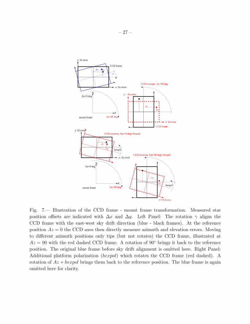
– 27 –
Az=0 deg
Az=90 deg
x: Az error
y: El error
CCD frame
x: El error
y: −Az error
mount frame
γ
CCD frame
∆
∆
x
y
CCD rotation: Az=90 deg
∆ ∆x y
N
E
Az=0 deg
Az=90 deg
x: Az error
mount frame
∆x
∆y
y: El errorCCD rotation: Az(=0 deg)+hexpol
hexpol
CCD frame
∆x
∆yhexpol
CCD rotation: Az(=90 deg)+hexpol
N
E
Fig. 7.— Illustration of the CCD frame - mount frame transformation. Measured star
position offsets are indicated with ∆x and ∆y. Left Panel: The rotation γ aligns the
CCD frame with the east-west sky drift direction (blue - black frames). At the reference
position Az = 0 the CCD axes then directly measure azimuth and elevation errors. Moving
to different azimuth positions only tips (but not rotates) the CCD frame, illustrated at
Az = 90 with the red dashed CCD frame. A rotation of 90◦ brings it back to the reference
position. The original blue frame before sky drift alignment is omitted here. Right Panel:
Additional platform polarization (hexpol) which rotates the CCD frame (red dashed). A
rotation of Az + hexpol brings them back to the reference position. The blue frame is again
omitted here for clarity.
– 28 –
15
10
5
0
5
10
15
15 10 5 0 5 10 15
tota
l raw
err
or in
eas
t-w
est d
irect
ion
[arc
min
]
total raw error in north-south direction [arcmin]
polar plot: total raw error - without IT
OT signatureraw error - without IT
15
10
5
0
5
10
15
15 10 5 0 5 10 15
tota
l raw
err
or in
eas
t-w
est d
irect
ion
[arc
min
]
total raw error in north-south direction [arcmin]
polar plot: total raw error - with IT
OT signatureraw error - with IT
Fig. 8.— Left Panel: Polar plot of the total raw error, combining ∆Azraw,k and ∆Elraw,k,
without IT correction. The remaining uncompensated OT collimation error (OT signature)
is shown as a circle which represents the OT tilt ∼ 9′ with respect to the mount pointing
axis. The data points scattered off the circle show the residual pointing errors ∆AzIT,k and
∆ElIT,k for the IT, leading to ∼ 1′ rms pointing error. The test was done with 250 stars.
Right Panel: Polar plot of the total raw error with IT correction. The OT collimation error is
again shown as a circle. The reduced scatter compared to the left panel verifies the improved
pointing with ∼ 0.4′ rms pointing error.
– 29 –
Fig. 9.— Left Panel: Front view of the AMiBA with a platform polarization hexpol = 0.
Installed are 7 antennas in compact configuration, giving 0.6m, 1.04m and 1.2m baselines.
Free receiver holes in the CFRP platform allow for different array configurations and for
a planned expansion phase with 13 antennas. The 8 inch refractor for optical pointing
is attached to the black bracket below the lowermost antenna at a distance of 1.4m from
the platform center. Right Panel: Front view of the AMiBA with a platform polarization
hexpol = 30. (Counter-clockwise rotation with respect to the left panel.)
– 30 –
-12
-10
-8
-6
-4
-2
0
2
4
6
8
10
0 1 2 3 4 5 6
raw
ele
vatio
n er
ror
[arc
min
]
azimuth [rad]
OT shifted to -20 degdata hexpol= -20 deg
OT fit at hexpol=0data hexpol= 0 deg
-12
-10
-8
-6
-4
-2
0
2
4
6
8
10
0 1 2 3 4 5 6
raw
ele
vatio
n er
ror
[arc
min
]
azimuth [rad]
OT shifted to -10 degdata hexpol= -10 deg
OT fit at hexpol=0data hexpol= 0 deg
-12
-10
-8
-6
-4
-2
0
2
4
6
8
10
0 1 2 3 4 5 6
raw
ele
vatio
n er
ror
[arc
min
]
azimuth [rad]
OT shifted to +10 degdata hexpol= +10 deg
OT fit at hexpol=0data hexpol= 0 deg
-12
-10
-8
-6
-4
-2
0
2
4
6
8
10
0 1 2 3 4 5 6
raw
ele
vatio
n er
ror
[arc
min
]
azimuth [rad]
OT shifted to +20 degdata hexpol= +20 deg
OT fit at hexpol=0data hexpol= 0 deg
Fig. 10.— Raw elevation errors (including remaining OT collimation error apparent as a
cosine-like signature) for hexpol = −20,−10,+10,+20◦, displayed in the panels from left to
right and top to bottom. An OT signature extracted from the hexpol = 0 pointing data is
shifted to the hexpol 6= 0 data to calculate the residual errors for the IT.
– 31 –
-4
-3
-2
-1
0
1
2
3
-20 -10 0 10 20
resi
dual
ele
vatio
n er
ror
[arc
min
]
polarization angle [deg]
polarization dependent elevation error for selected stars
star around Az=90 degstar around Az=180 degstar around Az=270 deg
star around Az=0 deg
Fig. 11.— Elevation error residuals after extracting the OT signature for selected stars at
Az=0, 90, 180, 270◦ as a function of hexpol. Errors tend to increase linearly towards larger
polarization angles. The azimuth errors (not shown) manifest the same result.
0
5
10
15
20
25
0 5 10 15 20 25 30
abso
lute
err
or w
rt to
initi
al p
ositi
on [a
rcse
c]
tracking time [min]
hexpol=constant tracking: cumulating tracking error
hexpol=constant cumulating tracking error
Fig. 12.— Tracking accuracy in hexpol=constant mode, accumulating linearly to a tracking
error of about 20′′ after 30 min.
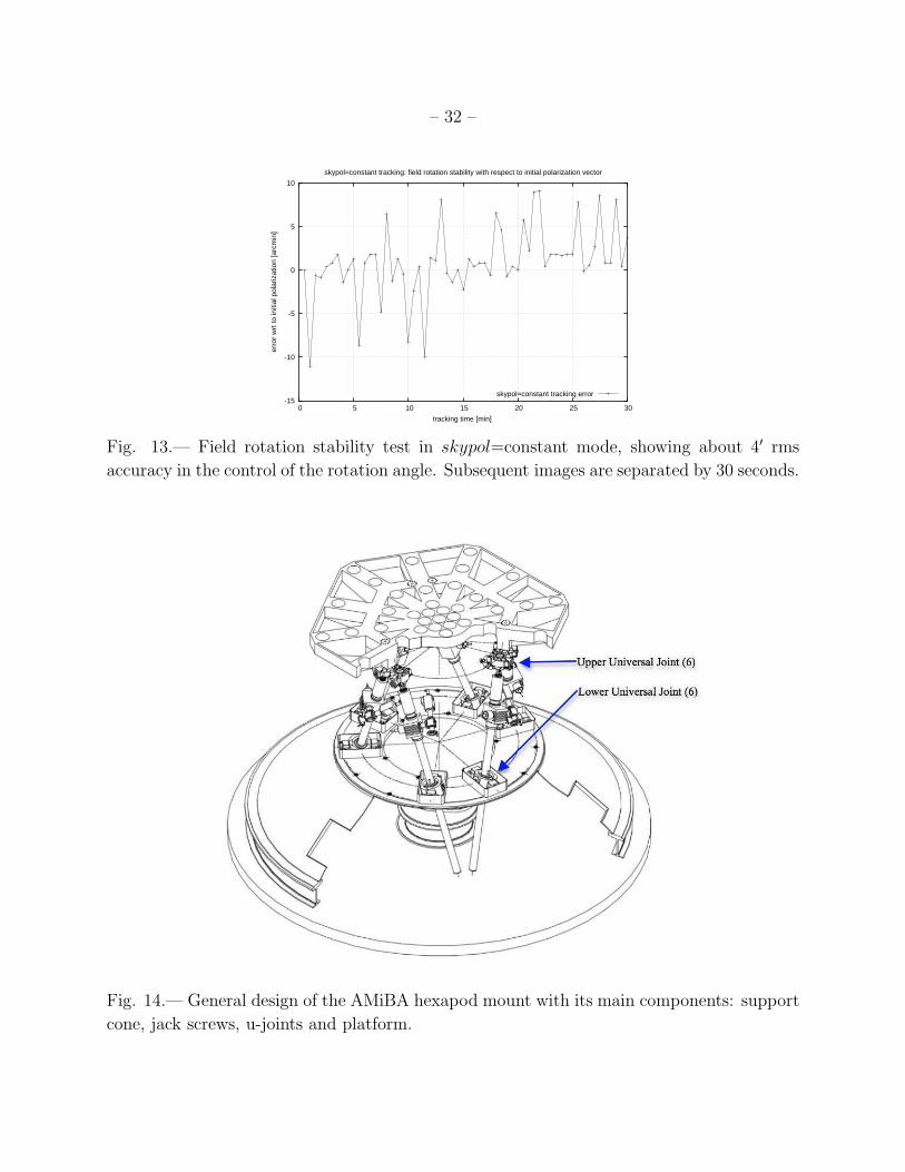
– 32 –
-15
-10
-5
0
5
10
0 5 10 15 20 25 30
erro
r w
rt to
initi
al p
olar
izat
ion
[arc
min
]
tracking time [min]
skypol=constant tracking: field rotation stability with respect to initial polarization vector
skypol=constant tracking error
Fig. 13.— Field rotation stability test in skypol=constant mode, showing about 4′ rms
accuracy in the control of the rotation angle. Subsequent images are separated by 30 seconds.
Fig. 14.— General design of the AMiBA hexapod mount with its main components: support
cone, jack screws, u-joints and platform.
– 33 –
Fig. 15.— The fundamental angles in astronomy and their relations in the mount and the
celestial coordinate systems.