insect-inspired, actively compliant robotic hexapod
TRANSCRIPT

INSECT-INSPIRED, ACTIVELY COMPLIANT ROBOTIC HEXAPOD
by
WILLIAM ANTHONY LEWINGER
Submitted in partial fulfillment of the requirements
For the degree of Master of Science
Thesis Advisers: Dr. Roger D. Quinn and Dr. Michael S. Branicky
Department of Electrical Engineering and Computer Science
CASE WESTERN RESERVE UNIVERSITY
May, 2005

ii
CASE WESTERN RESERVE UNIVERSITY
SCHOOL OF GRADUATE STUDIES
We hereby approve the thesis/dissertation of ________________________________________________________ candidate for the __________________________________ degree. (signed)_________________________________________________ (Chair of the Committee)
_________________________________________________ _________________________________________________ _________________________________________________ _________________________________________________ _________________________________________________
(Date) ____________________

iii
Copyright © by William Anthony Lewinger All rights reserved

iv
I grant to Case Western Reserve University the right to use this work, irrespective of any copyright, for the University’s own purposes without cost to the University or to its students, agents and employees. I further agree that the University may reproduce and provide single copies of the work, in any format other than in or from microforms, to the public for the cost of reproduction.
(sign)

v
This thesis is dedicated to Kim, who got me started in grad school; to Julie, who helped me get through it all in one piece; and to my parents, who supported me throughout the whole process.
"The spacecraft has apparently been taken over – "conquered" if you will – by a master race of giant space ants. It's difficult to tell from this vantage point whether they will consume the captive earth men or merely enslave them. One thing is for certain: there is no stopping them; the ants will soon be here. And I for one welcome our new insect overlords. I'd like to remind them that as a trusted TV personality I could be helpful in rounding up others to toil in their underground sugar caves." – Kent Brockman

1
TABLE OF CONTENTS
TABLE OF CONTENTS ............................................................................................................1
LIST OF TABLES ....................................................................................................................5
LIST OF FIGURES ...................................................................................................................6
LIST OF FUNCTIONS ..............................................................................................................8
LIST OF ABBREVIATIONS.....................................................................................................10
GLOSSARY ..........................................................................................................................11
CHAPTER I ..........................................................................................................................15
Introduction............................................................................................................15
1.0 General.......................................................................................................15
1.1 Goals ..........................................................................................................18
1.2 Thesis Contributions ..................................................................................18
1.3 Chapter Topics ...........................................................................................19
CHAPTER II .........................................................................................................................21
Review of Previous Research ................................................................................21
2.0 General.......................................................................................................21
2.1 Hexapod Robot Kits...................................................................................22
2.2 Hexapod Robots.........................................................................................23
2.2.1 Tarry I and Tarry II ........................................................................23
2.2.2 Robot II ..........................................................................................25
2.2.3 TUM Walking Machine.................................................................27
2.2.4 Additional 18-DOF Hexapod Robots ............................................29

2
CHAPTER III........................................................................................................................31
Mechanical System ................................................................................................31
3.0 General.......................................................................................................31
3.1 Body...........................................................................................................32
3.2 Legs............................................................................................................35
3.3 Neck, Head and Mandibles ........................................................................41
CHAPTER IV........................................................................................................................45
Electrical System ...................................................................................................45
4.0 General.......................................................................................................45
4.1 IsoPod™ Programmable Servo Control Board..........................................45
4.2 BrainStem Microcontroller ........................................................................48
4.3 System Controller ......................................................................................49
4.4 Power System.............................................................................................50
CHAPTER V.........................................................................................................................53
Software System ....................................................................................................53
5.0 General.......................................................................................................53
5.1 Software Interface......................................................................................53
5.2 Cruse Controller: Overview, Methodology, and Implementation .............60
5.3 Determining Cruse Mechanism Weights and Bias Values ........................65
5.4 Standing .....................................................................................................71
5.5 Movement: Walking, Strafing, and Rotating.............................................72
5.6 Body Posture: Height, Pitch, and Roll .......................................................78
5.7 Force Feedback Sensors and the Affects on Movement and Posture ........79

3
5.8 Control and Autonomy ..............................................................................81
CHAPTER VI........................................................................................................................83
Project Development and Evolution ......................................................................83
6.0 General.......................................................................................................83
6.1 One-Leg Test Rig.......................................................................................83
6.2 Basic IsoPod™ Interfacing ........................................................................85
6.3 Two-Leg Test Platform and Software Interface ........................................86
6.4 Initial Six-Leg Platform and Software Interface........................................90
6.5 Current Six-Leg Platform and Software Interface .....................................93
6.6 Control and Autonomy ..............................................................................93
6.7 Prototype Mandibles ..................................................................................94
CHAPTER VII ......................................................................................................................95
System Performance ..............................................................................................95
7.0 General.......................................................................................................95
7.1 System Component Masses .......................................................................95
7.2 Lifting and Sustaining Load Capacities.....................................................96
7.3 Walking Load Capacity .............................................................................98
7.4 Driving and Turning Performance .............................................................99
7.5 Body Movement in Response to External Forces......................................99
7.6 Battery Life and Power ............................................................................100
CHAPTER VIII...................................................................................................................101
Future Work .........................................................................................................101
8.0 General.....................................................................................................101

4
8.1 On-board Control, Navigation, and Communication...............................101
8.2 Event-Based Broadcast Communication .................................................102
8.3 Leader and Helper Roles..........................................................................103
8.4 Helper Role Bidding Process ...................................................................104
LIST OF REFERENCES ........................................................................................................105
APPENDICES......................................................................................................................109
APPENDIX A – BILL-ANT-P DRAWINGS ...........................................................................109
APPENDIX B – MATERIALS LISTS AND COSTS...................................................................121

5
LIST OF TABLES
Table 1. 18-DOF hexapod robot general information chart. ............................................29
Table 2. 18-DOF hexapod robot specifications comparison chart (Berns 2005). ............30
Table 3. Component and subsystem masses. ....................................................................96
Table 4. Robot lifting load capacities on carpeted surface. ..............................................97
Table 5. Robot lifting load capacities on smooth surface.................................................97
Table 6. Robot sustaining load capacities on carpeted surface.........................................98
Table 7. Robot sustaining load capacities on smooth surface. .........................................98
6
LIST OF FIGURES
Figure 1. BILL-Ant-p robot (without the neck, head, and mandibles) ...........................17
Figure 2. Tarry I (left) and Tarry II (right) built by the Department of Engineering
Mechanics at the University of Duisberg (Buschmann 2000a). ......................24
Figure 3. Robot II built by the Biorobotics Lab in the Department of Mechanical and
Aerospace Engineering at Case Western Reserve University (Espenschied et
al. 1996). ..........................................................................................................26
Figure 4. TUM Walking Machine built by Dr. Friedrich Pfeiffer at Technische
Universität München (Berns 2005)..................................................................28
Figure 5. Acromyrmex versicolor (left, Leafcutter ant found in Arizona, USA, ©Dale
Ward) and BILL-Ant-p (right) body parts. ......................................................31
Figure 6. Robot body section without electronics or batteries. .......................................33
Figure 7. Top-view body layout comparison of Pheidole fervida (left, found in Japan,
©Japanese Ant Database Group) and the BILL-Ant-p robot (right). ..............34
Figure 8. Front left leg attached to the body. ..................................................................36
Figure 9. Machined coxae with body-coxa joint axles installed. ....................................38
Figure 10. Double yoke femurs. .......................................................................................39
Figure 11. Foot assembly and force transducer characteristics. .......................................41
Figure 12. Rendering of the head and neck assembly with attached mandibles...............42
Figure 13. Pincer-mounted force-sensitive resistor assembly. .........................................44
Figure 14. Electronic and control system connectivity.....................................................45
Figure 15. New Micros, Inc. IsoPod™ microcontroller with attached daughterboard
(©New Micros, Inc.)........................................................................................46

7
Figure 16. Acroname BrainStem GP 1.0 microcontroller (©Acroname, Inc.). ................49
Figure 17. User interface with Drive Control window shown..........................................54
Figure 18. Inverse kinematics calculation flow chart. ......................................................56
Figure 19. Cruse’s basic rule set for stick insect walking (Schmitz 1998).......................61
Figure 20. Foot path and signal forms for Mechanisms 1, 2, and 5 with respect to leg
position.............................................................................................................62
Figure 21. Leg motion during a standing cycle. ...............................................................72
Figure 22. Drive cycle flow chart. ....................................................................................73
Figure 23. Foot state (swing/stance) as speed increases. ..................................................74
Figure 24. Walking (left), strafing at 330º (center), and CCW rotating (right) foot paths
(arrows indicate foot swing direction). ............................................................75
Figure 25. One-leg test rig. ...............................................................................................84
Figure 26. Two-legged test platform with the attached stand...........................................87
Figure 27. Two-legged test platform user interface..........................................................89
Figure 28. Initial six-legged test platform user interface..................................................91
Figure 29. Prototype mandibles closed and open as viewed from the bottom. ................94

8
LIST OF FUNCTIONS
Function 1. Forward kinematics equation.........................................................................57
Function 2. PEP adjustment function segment for leg 0 (front right leg).........................64
Function 3. Function to set mechanism weights and bias values for evaluation. .............67
Function 4. Function to adjust mechanism weights and bias values for evaluation. ........68
Function 5. Assign scores to the current set of weight and bias values............................70
Function 6. Calculate individual foot headings and assign new AEP and base PEP
coordinate values. .........................................................................................77
Function 7. Calculate external force magnitude and direction, and move in the direction
of the force vector, relative to the body center. ............................................81

9
Acknowledgements
Arnold Lewinger for having five TVs in the house when I was growing up (one of which actually worked) and teaching me to solder at the age of 12; and Jean Lewinger for getting scared by a Radio Shack® 75-in-one kit that I had modified to make machine gun sounds (also when I was about 12), suggesting my potential for evil genius.
The U.S. Naval Nuclear Power Program for giving me the engineering background and personal determination to see myself through any project.
Dr. Robert Avanzato (Penn State, Abington) for dropping a box of Lego® bricks and an MIT 6.270 microcontroller on a table and saying “figure it out”.
Dr. Michael Branicky for becoming my impromptu advisor and getting me into the Neuromechanics program.
Dr. Roger Quinn for being a source of constant support and an advisor for the mechanical engineering aspects of the design. Also for providing space for me in the Biorobotics Laboratory and access to the wonderful machining tools.
Tom Allen and Terence Wei for introducing me to the machine shop (and the fantastic Hurco CNC machine) and teaching me enough so that I didn’t cut off anything important (unless I meant to).
Dan Kingsley and (unknowingly) Ken Espenschied for providing explanation and insight into the Cruse controller.
The Biorobotics Lab students not mentioned above for all their help and support: Kurt Aschenbeck Rich Bachmann Alex Boxerbaum
Jong-Ung Choi Kati Daltorio Andy Horchler Nicole Kern Bram Lambrecht Brandon Rutter
The IGERT-NSF fellowship for providing the funding that made pursuit of this degree this possible.

10
LIST OF ABBREVIATIONS
ADC Analog-to-Digital Converter
AEP Anterior Extreme Position
ANN Artificial Neural Network
BC Joint Body-Coxa Joint
CF Joint Coxa-Femur Joint
DOF Degree(s) of Freedom
FT Joint Femur-Tibia Joint
I/O Input/Output
I2C Inter-IC Communication Interface
IR Infrared
NiMH Nickel Metal Hydride
PEP Posterior Extreme Position
PEPa Adjusted Posterior Extreme Position
PWM Pulse Width Modulation
R/C Radio Control, Radio Controlled
µC Microcontroller

11
GLOSSARY
BC Joint
See Body-Coxa Joint.
Body
This is the main portion of the robot. It houses the batteries and leg control microcontroller, and provides connection points for the BC Joints and Neck.
Body-Coxa Joint (BC Joint, Swing Joint)
The first (most proximal) joint and degree-of-freedom for each leg. Connecting the body and Lift Bracket, it consists of an inverted-mounted R/C servo motor and controls leg swing.
BrainStem
See BrainStem Microcontroller.
BrainStem Microcontroller (BrainStem)
Programmable microcontroller with four R/C servo ports, five ADC input ports, five digital I/O ports, and RS-232 and I2C interfaces, used to control the neck and mandibles.
CF Joint
See Coxa-Femur Joint.
Coxa-Femur Joint (CF Joint, Lift Joint)
The second (middle) joint and degree-of-freedom for each leg. Connecting the Lift Bracket and the femur, it consists of a horizontally-mounted R/C servo motor and controls leg lift.
Femur
Leg segment between the body and knee. It consists of two parallel carbon fiber plates separated by an aluminum strut, and is shaped like a double yoke.

12
Femur-Tibia Joint (FT Joint, Knee Joint)
The third (most distal) joint and degree-of-freedom for each leg. Connecting the femur and the tibia, it consists of a horizontally-mounted R/C servo motor and controls knee bending.
Foot
Two parallel aluminum plates housing a force-resistive sensor for measuring leg loads, and is attached to the distal end of the tibia.
FT Joint
See Femur-Tibia Joint.
IsoPod™
See IsoPod™ Microcontroller.
IsoPod™ Microcontroller (IsoPod™, Servo Controller, Leg Control Microcontroller)
Microcontroller and interface board by New Micros, Inc. (Dallas, TX, USA). This board controls up to 26 R/C servos (with the attached daughter board), has eight ADC input ports, on-board memory and programmability, two RS-232 serial ports, and additional interfaces.
Knee Joint
See Femur-Tibia Joint.
Leg Control Microcontroller
See IsoPod™ Microcontroller.
Lift Bracket
An aluminum housing that holds the CF Joint R/C servo motor and provides a connection point for the BC Joint.
Lift Joint
See Coxa-Femur Joint.

13
Mandibles
Aluminum pincers attached to the head and actuated by an R/C servo, capable of grasping objects.
Microcontroller
See IsoPod™ Microcontroller or BrainStem Microcontroller.
Pulse Width Modulation (PWM)
A method of adjusting the average dc voltage by varying the amount of time that voltage is maximum, and zero otherwise, within a fixed period of time. For R/C servos, a special type of PWM is used with a period of 2-50msec. During the period, voltage is set to maximum (4.8-6.0vdc) for between 1.1msec and 1.9msec to achieve the full range of motion of the servo. 1.5msec is the neutral or middle position.
R/C Servo
See R/C Servo Motor.
R/C Servo Motor (R/C Servo, Servo Motor, Servo)
Standard-size MPI MX-450HP radio control dc servo motor, used in all joints on the robot.
Servo
See R/C Servo Motor.
Servo Controller
See IsoPod™ Microcontroller.
Servo Motor
See R/C Servo Motor.
Swing Joint
See Body-Coxa Joint.
Tibia
Distal leg segment between the knee and foot; made of aluminum.

14
Insect-Inspired, Actively Compliant Robotic Hexapod
Abstract
by
WILLIAM ANTHONY LEWINGER
Insects, in general, are agile creatures capable of navigating uneven and difficult terrain
with ease. The leaf-cutter ants (Atta), specifically, are agile, social insects capable of
navigating uneven and difficult terrain, manipulating objects in their environment,
broadcasting general event messages to other leaf-cutter ants, performing collective tasks,
and operating in cooperative manners with others of its kind. These traits are desirable in
a mobile robot. However, no robots have been developed that encompass all of these
capabilities. As such, this research developed the Biologically-Inspired Legged-
Locomotion Ant prototype (BILL-ANT-p) to fill the void.
This thesis discusses the features, development, and implementation of the BILL-Ant-p
robot, quantifies its capabilities for use as compliant mobile platform, and defines future
features that enable social behavior and cooperative object manipulation.

15
CHAPTER I
INTRODUCTION
1.0 General
Ultimately, it is the goal of this research is to develop a robot that is power and
control autonomous; capable of navigating uneven terrain, manipulating objects
within the environment, working together cooperatively, and employment of
compliance with the environment and other robots; very strong for its size; and is
relatively inexpensive compared to other similar robots.
When thinking of sources of inspiration for this topic, one of the first things that
come to mind are insects, especially ants. Ants are agile, social creatures that
navigate and manipulate their environment with ease (Hölldobler and Wilson
1990; Yahya 2000). With limited individual abilities, ants perform greater tasks
by working cooperatively with one another (Hölldobler and Wilson 1990; Yahya
1990). As such, they seemed the perfect model on which to base a robot design.
The leaf-cutter ant (Atta), in particular, fits the essence of this research. Agile,
social, able to communicate with others of its kind with broadcast messages, and
capable of gathering objects in its environment and returning them to the nest, the
leaf-cutter ant is an ideal model (Yahya 2000).
There are, however, limitations to the degree of biological inspiration that can
realistically be implemented in robots; see (Webb 2001) and its references.

16
Biological creatures have muscles which are much stronger for their size than
comparable mechanical actuators, body tissue is stronger and lighter in weight
than artificial materials would be, and (in the case of ants) they are quite tiny.
Because of these limitations, compromises need to be made. To aid in deciding
which features are to be implemented in an artificial robot, an analysis of the
physical and social characteristics of the ant was performed.
Which features of the leaf-cutter ant and other insects are desirable for this
research? 1. They use six legs to move with agility over difficult terrain, so the
robot must be capable of stable walking in any direction on uneven terrain. A
hexapod with at least three degrees-of-freedom per leg could accomplish this
(Espenschied et al. 1995; Espenschied et al. 1996). Hexapods with fewer degrees
of freedom cannot move dynamically in any direction, and robots with greater
degrees of freedom weigh more, consume more power, require additional control
complexity, and are more expensive. 2. They haves mandibles that can chew and
carry food. Mechanical mandibles would be required to fill this function. 3.
Ants, in particular, are social insects that can operate cooperatively with others,
including assisting one another, at times, with carrying objects (Yahya 2000).
This can be implemented through software whereby two or more robots can assist
each other while moving a single object. 4. Also, the leaf-cutter ant
communicates with its neighbors by creating vibrations with its body,
“stridulation”, that propagate through the substrate (Hölldobler and Wilson 1990;
Roces et al. 1993; Roces and Hölldobler 1995; Tautz et al. 1995; Roces and
Hölldobler 1996). This feature seemed impractical to implement directly,

17
however, short-range wireless communication that can be broadcast without a
specifically intended recipient could be used instead.
With these criteria in mind, research was conducted into any existing robots with
such capabilities. There are other robots that use wheels on flat, smooth surfaces
that manipulate objects, such as Dr. Chris Melhuish’s U-Bots (Melhuish et al.
1998), and other techniques for object manipulation by sliding (Matarić 1995).
There are also a whole host of legged robots and hexapods. However, there are
no insect-inspired object-grasping cooperative legged robots. So, development
began on the Biologically-Inspired Legged-Locomotion Ant prototype (BILL-
Ant-p) (Fig. 1) that would be able to perform all of the desired tasks listed above.
Figure 1. BILL-Ant-p robot (without the neck, head, and mandibles)

18
1.1 Goals
There were several goals at the onset of this project.
Design and build a robot:
• That is similar in physical design to an ant
• With the ability to walk in any direction (strafe) and rotate, at the same
time if needed
• That is strong enough to stand up with another robot on its back
• That is power and control autonomous
• With mandibles for object manipulation
• That can cooperatively transport a carried object with another robot
• With active and/or passive compliance with the ground and grasped
objects
• That is capable of communicating with other similar robots wirelessly
• That is relatively inexpensive
1.2 Thesis Contributions
This thesis contributed the following:
• Created a design for an 18-DOF hexapod robot with autonomous power
and the capacity for autonomous control

19
• Constructed a functional 18-DOF hexapod capable of straight-line
walking, strafing, rotating, and combined strafing/rotating using a Cruse
controller for leg coordination
• Developed and implemented an active compliance body movement
controller in response to external forces through measurements taken from
foot-mounted force sensors
• Created a graphical user interface capable of controlling: individual joint
movement; foot position in body-centric coordinates; body posture such as
ground clearance, pitch, and roll; a pre-programmed standing routine;
walking movements through speed, heading, and rotation; active
compliance behavior; and displaying foot-mounted force sensor data
• Quantified performance data for the BILL-Ant-p robot as an actively-
compliant 18-DOF hexapod
1.3 Chapter Topics
Chapter 1, this chapter, is the introduction and discusses the research background,
goals, contributions, and a list of topics for subsequent chapters.
Chapter 2 discusses desirable robot characteristics, reviews existing robots, and
identifies and compares similar robots.
Chapter 3 covers the design and implementation of the mechanical aspects of the
BILL-Ant-p robot.
Chapter 4 includes electronic control processors and the electrical power system.
20
Chapter 5 details the project development and evolution from initial joint motor
testing to the present 18-DOF hexapod.
Chapter 6 quantifies various system weights and performance values.
Chapter 7 describes future work.

21
CHAPTER II
REVIEW OF PREVIOUS RESEARCH
2.0 General
Several criteria are needed to achieve coordinated object manipulation over
uneven terrain: the ability to navigate uneven terrain, the ability to manipulate
objects, the ability to maintain a fixed position relative to another robot while that
robot moves freely. The third criterion requires robots that can move in one
direction while potentially facing another (strafing or crabbing) (Espenschied et
al. 1995; Espenschied et al. 1996). While not an inherent movement mode in
ants, strafing was deemed necessary for multiple robots to move a rigid object. In
addressing the criteria, certain physical traits are required and discussed below.
Legged robots have the ability to move over uneven and discontinuous terrain
with more agility than wheeled or tracked vehicles (Espenschied et al. 1995;
Espenschied et al. 1996). Also, within the legged robot community, only robots
with at least three degrees-of-freedom per leg are capable of strafing movements
such as crabbing (1- and 2-DOF legs can only move in one and two dimensions,
respectively; To move in three dimensions, at least three degrees-of-freedom are
required). So, robots such as Robot I (Espenschied and Quinn 1994) and Genghis
(Brooks 1989), which have 2-DOF legs, were not considered. Bipeds,
quadrupeds, hexapods, and octopods are all potentially capable of performing the
required movements. However, bipeds and quadrupeds are less stable, so they

22
were not considered as vehicle candidates. Six- and eight-legged robots are
naturally stable, even while in motion; however, the additional two legs of
octopods were considered redundant, are more heavier and complex, and require
more power and computational control. Also, robots with more than 3-DOF per
leg were discounted since they require extra amounts of control and provide
unnecessary additional joints. As such, only 18-DOF hexapod robots were
considered. Also, the robots discussed below all use the Cruse control model.
Four examples of such hexapods are described in Section 2.2.
2.1 Hexapod Robot Kits
With the desire to minimize the amount of effort required to create a mobile
legged platform capable of object manipulation, two hexapod kits were
considered: the Lynxmotion, Inc. (Pekin, IL, USA) Hexapod 3 and the
Micromagic Systems (Winchester, Hanst, UK) PyEbot V2 Hexapod.
The Lynxmotion, Inc. robot uses Hitec HS-475HB servo motors (Hitec RCD,
Inc., Poway, CA, USA) to actuate the leg joints. These servos are capable of
61oz.-in. (4.4 kg-cm) of torque and a speed of 0.23sec for 60º of rotation. This is
approximately half of the torque and 2/3 of the speed of the MPI-450HP servo
motors (Maxx Products, Inc., Lake Zurich, IL, USA) used in the BILL-Ant-p.
Also, the Lynxmotion, Inc. hexapod is crafted from 0.125in. (3.18mm) thick
Lexan®, and is not sufficiently durable for lifting heavier objects.

23
The Micromagic Systems hexapod uses smaller and less powerful servo motors
than the Lynxmotion, Inc. robot, also uses polycarbonate body parts, but was not
available for purchase at the time research began.
Neither the kits nor the hexapods described below are capable of carrying an
object in their current forms. While research has been done with puck sorting and
object manipulation through pushing (Melhuish et al. 1998; Matarić 1995), this
project requires that an object can be grasped and elevated over rough terrain. As
such, neither of the hexapod kits nor the other existing research robots was
selected, and an original design was initiated instead.
2.2 Hexapod Robots
Here, four hexapod robots are described that are very similar to the BILL-Ant-p in
number of legs and joints, use of a Cruse-based leg controller, and in the case of
Tarry I and Tarry II use of hobby servo motors for joint actuation.
2.2.1 Tarry I and Tarry II
Based on the stick insect (Carausius morosus), development of Tarry I (Fig. 2,
left) began in 1992 by the Department of Engineering Mechanics at the University
of Duisberg, and was headed by Dr. Martin Frik. The goal was to develop an
autonomous six-legged walking vehicle to navigate smooth and uneven terrains
while under operator control, and to autonomously explore and determine what
path to take when moving to a pre-defined goal (Buschmann 2000a). Similar to

24
the BILL-Ant-p robot, Tarry I uses hobby R/C servo motors for the leg joints and
has 18 degrees-of-freedom.
In 1998, development of Tarry II (Fig. 2, right) began. Tarry II is similar to Tarry
I, but more loosely based on the stick insect. It uses more powerful servo motors
and some other slight design differences. While Tarry I uses stick insect
proportions for relative leg placement and segment lengths, Tarry II uses
dimensions that reduce mechanical strain (Buschmann 2000a).
Figure 2. Tarry I (left) and Tarry II (right) built by the Department of
Engineering Mechanics at the University of Duisberg (Buschmann 2000a).
Tarry I and Tarry II also have foot contact switches, instead of the force-sensing
resistors used in the BILL-Ant-p robot, and measures power consumed by the leg
actuators to detect collisions. Also, a front-mounted ultrasonic sensor is used to
detect large obstacles. The robots also employ strain gauges attached to the legs

25
for measuring strains during movement, and an inclinometer to maintain a
horizontal body posture (Buschmann 2000a).
The Tarry series uses an implementation of the Cruse controller called Walknet,
an artificial neural network (ANN) (Cruse et al. 1993). Walknet is trained to
control walking tasks such as straight walking at different speeds, walking in
curves, and walking in different directions (strafing).
Tarry II also uses off-board power and off-board control, but will be later
developed with on-board batteries and an on-board PC/104 controller for
demonstration purposes (Buschmann 2000b).
Tarry I is approximately 19.7in. (50cm) long, 15.7in. (40cm) wide, 7.1in. tall
(18cm), weighs 4.60lbs (2092g), and can support a payload of 0.88lbs. (400g).
Tarry II is approximately 19.7in. (50cm) long, 19.7in. (50cm) wide, 7.9in. tall
(20cm), weighs 6.39lbs. (2905g), and can support a payload of 6.38lbs. (2900g)
(Buschmann 2000a).
2.2.2 Robot II
At the Case Western Reserve University Biorobotics Lab in 1993, development
began on Robot II (Fig. 3), a stick insect-inspired, 18 active degree-of-freedom
(six passive DOF) actuated hexapod robot (Espenschied and Quinn 1994;
Espenschied et al. 1994; Espenschied et al. 1995; Espenschied et al. 1996). Robot
II uses insect-like reflexes for each leg to navigate uneven and discontinuous
terrain independently of one another.

26
The gait controller for Robot II was adapted from the network published by Cruse
and Dean, which was based on stick insect leg coordination (Cruse et al. 1993). A
continuous range of static gaits is generated as speed increases, like in the BILL-
Ant-p, over flat terrain. When encountering discontinuous terrain and obstacles,
Robot II employs two insect-like behaviors to navigate successfully: a searching
reflex and an elevator reflex, respectively (Espenschied et al. 1995; Espenschied
et al. 1996).
Figure 3. Robot II built by the Biorobotics Lab in the Department of Mechanical
and Aerospace Engineering at Case Western Reserve University
(Espenschied et al. 1996).
On discontinuous surfaces, such as a slatted walkway, the searching reflex is
initiated when the passive force sensor in the tibia fails to detect the ground at the

27
expected level. An iterative cycle of searching downward and forward for a
foothold begins, where a pattern of ever-increasing radii circles is used for a fixed
number of cycles.
If an obstacle is detected, the elevator reflex is initiated and reverses the leg
direction and proceeds forward again at a higher elevation. This process is
repeated up to a height of 3.15in. (8cm).
Like the Tarry series, Robot II uses external power and an external leg
coordination control system. Unlike the Tarry robots and the BILL-Ant-p robot,
however, Robot II uses 18 6-Watt Maxon motors (Maxon Motor AG, Sachseln,
Switzerland) and position feedback potentiometers for the actuated joints, instead
of hobby servo motors, and employs an external motor control system to set
position, velocity, and stiffness of each actuator. Robot II is 19.7in. (50cm) long,
19.7in. (50cm) wide, and 9.8in. (25cm) tall (Espenschied et al. 1996).
2.2.3 TUM Walking Machine
Dr. Friedrich Pfeiffer at Technische Universität München began work on the
TUM Walking Machine (Fig. 4) in 1991 (Berns 2005). This robot, like the others
listed above, is based on the stick insect and uses a form of Cruse control for leg
coordination (Pfeiffer et al. 1994). Like the Tarry series and Robot II, the TUM
Walking Machine uses distributed leg control so that each leg may be self-
regulating with influences from adjacent legs.

28
However, unlike the previous robots and the BILL-Ant-p robot, the TUM
Walking machine only uses Mechanism 1 from the Cruse model: “A leg is
hindered from starting its return stroke while its posterior leg is performing a
return stroke” (Barnes 1998) and is applied to ipsilateral and contralateral
adjacent legs. The original Cruse model only applies the influences of
Mechanism 1 to the ipsilateral leg in front of the current leg (Fig. 19).
Additionally, a leg was prevented from entering the swing phase while any
adjacent neighboring legs were also in swing.
Figure 4. TUM Walking Machine built by Dr. Friedrich Pfeiffer at Technische
Universität München (Berns 2005).
The TUM Walking machine is 31.5in. (80cm) long, 39.4in. (100cm) wide, and
15.7in. (40cm) tall (Berns 2005).

29
2.2.4 Additional 18-DOF Hexapod Robots
Many other motor-actuated 18-DOF hexapod robots have been built over the
years, some of which are listed in Table 1 along with the previously mentioned
robots. Table 2 compares general specifications of the mentioned robots with the
BILL-Ant-p robot.
Robot Head Professor Institute Selected References
Attila II Dr. Rodney Brooks
MIT Angle 1991; Ferrell 1993
LAURON LAURON II LAURON III
Dr. Karsten Berns Forschungszentrum Informatik
Gaßmann et al. 1991
Robot II Dr. Roger Quinn Case Western Reserve University, Biorobotics Lab
Espenschied and Quinn 1994; Espenschied et al. 1995
Tarry I Tarry II
Dr. Martin Frik University of Duisberg
Buschmann 2000a
TUM Walking Machine
Dr. Friedrich Pfeiffer
Technische Universität München
Pfeiffer et al. 1994
Table 1. 18-DOF hexapod robot general information chart.

30
Rob
ot
BIL
L-A
nt-p
Atti
la II
LAU
RO
N
LAU
RO
N II
LAU
RO
N
III
Rob
ot II
Tarr
y I
Tarr
y II
TUM
W
alki
ng
Mac
hine
Length 0.33m 0.36m 0.8m 0.7m 0.5m 0.5m 0.4m 0.5m 0.8m
Width 0.33m 0.20m 0.3m 0.3m 0.3m 0.25m 0.15m 0.2m 0.4m
Height 0.15m 0.31m 0.7m 0.7m 0.8m 0.5m 0.3m 0.4m 1.0m
Max. Speed
0.004m/s 0.8m/s 1.0m/s 0.5m/s 0.4m/s 0.14m/s 0.15m/s 0.20m/s 0.3m/s
Weight 2.3kg 1.5kg 12kg 16kg 18kg -- 2.2kg 2.9kg 23kg
Load 8.6kg 150g 1kg 15kg 10kg -- 0.3kg 2.9kg 5kg
Legs 6 6 6 6 6 6 6 6 6
Active Degrees
18 18 18 18 18 18 18 18 18
Passive Degrees
6 6 0 0 0 6 0 0 0
Energy Supply
DC Servos -- DC
Servos DC
Servos DC
Servos DC
Motors DC
Servos DC
Servos DC
Motors
Power Supply
6V Batteries 12V 12V 12V 12V -- 12V --
Power Consump.
20W -- 90W 70W 90W -- 30W 30W 500W
Table 2. 18-DOF hexapod robot specifications comparison chart (Berns 2005).

31
CHAPTER III
MECHANICAL SYSTEM
3.0 General
The BILL-Ant-p robot is divided into three major sections: body, legs, and
head/neck (Fig. 5). Each section is constructed from a 6061 aluminum frame
(thickness varying with section) and 0.0625in. (1.59mm) thick carbon fiber sheets
(McMaster-Carr Supply Co., Cleveland, OH, USA). These materials were chosen
for their balance of strength and light weight.
Figure 5. Acromyrmex versicolor (left, Leafcutter ant found in Arizona, USA,
©Dale Ward) and BILL-Ant-p (right) body parts.
Designs were initially created using Autodesk’s AutoCAD 14 (Autodesk, Inc.,
San Rafael, CA, USA). All virtual prototyping for form, placement, range-of-
motion, and interconnectivity was also done with AutoCAD.

32
Once the preliminary designs were complete, physical prototyping was
performed. Initial parts were created by hand using standard machining tools.
These parts were evaluated in limited-functionality versions of the robot, such as
a body portion with only two legs (see Section 6.3). Once evaluations of those
parts were finished, the designs were updated in AutoCAD and created with
PTC’s Pro/Engineer 2001 (Parametric Technology Corp., Needham, MA, USA).
Using the CNC exportation feature, these parts were then converted into
manufacturing files for fabrication by a Hurco VM1 Machining Center (Hurco
Companies, Inc., Indianapolis, IN, USA).
3.1 Body
The body is the main section of the robot and is used as the anchor point for the
legs and neck, and houses the power supplies (internally) and leg control
electronics (mounted to the top) (Fig. 6). It is 6.62in. (16.8cm) wide, 8.60in.
(21.8cm) long, and 1.93in. (4.90cm) tall at the extreme points and is constructed
from a hollow 0.1875in. (4.76mm) thick 6061 aluminum frame and two 0.0625in.
(1.59mm) thick carbon fiber plates.
The internal skeleton consists of the spine, front face plate, rear face plate, and
two supporting square C-shaped ribs. Each piece is 0.1875in. (4.76mm) thick,
1.80in. (4.57cm) tall 6061 aluminum and has been hollowed to reduce weight.
The front and rear face place holes (Fig. 6) are used to insert the four Li-ion
batteries. The skeleton parts are connected with 2-56 18-8 stainless steel button
socket hex head cap screws.

33
Figure 6. Robot body section without electronics or batteries.
Top and bottom plates are 0.0625in. (1.59mm) thick carbon fiber sheets that are
secured to the skeleton, giving the body additional rigidity. The square (Fig. 6 top
plate) and round (Fig. 6 bottom plate) holes are used to mount the body-coxa
servo motors in an inverted position and support the joint axles, respectively.
Layout of the body and orientation of the BC joints was based as closely as
possible to the body segments of various ants (Fig. 7). While the ant has a much
more body compact configuration, the mechanical design was limited by the
constraints of function (housing batteries and servo controller) and the connecting
elements (legs and head/neck). Leg placement and orientation was designed to
accommodate 90 degrees of rotation for each BC joints (maximum range of
motion for the joint motors) without interfering with other legs throughout the
range of motion. Front and rear body-coxa servos are splayed 60 degrees from

34
the medial plane. The middle BC joint motors are perpendicular to the medial
plane. This pattern is similar to the ant for the middle and rear legs; however, it is
not biologically accurate for the front legs. While the front body-coxa servo
orientations were chosen to produce axially-symmetric body plates, the front legs
are attached to their respective servos to roughly conform to the ant’s anatomy
with a starting position of 15 degrees from the medial plane. All legs have ±45
degrees of motion; however the front legs have +0/-90 degrees of
forward/rearward motion from starting positions of 15 degrees off the medial
plane.
Figure 7. Top-view body layout comparison of Pheidole fervida (left, found in
Japan, ©Japanese Ant Database Group) and the BILL-Ant-p robot (right).

35
Body height (1.93in./4.90cm) was designed to be as small as possible while still
accommodating the Li-ion batteries internally. Due to the limited amount of
space on the sides when the legs are present, the batteries are inserted and
removed through the front and rear face plates. Internal holders (not shown in
Fig. 6) are used to support the batteries and the voltage conditioning units.
3.2 Legs
There are six 3-DOF legs on the BILL-Ant-p robot. Three degrees-of-freedom
were chosen as that is the minimum number which allows strafing; a desired trait
for the robot to enable more agile movements. Additional DOF would have been
redundant for basic walking and would have required a greater amount of
complexity, power, and processing to control.
Each leg consists of three joints and four segments (Fig. 8). The first joint is the
body-coxa (BC) joint, which swings the coxa forward and rearward in the body’s
dorsal plane. Next is the coxa-femur (CF) joint, which raises and lowers the
femur in the leg-based medial plane. Finally, the femur-tibia (FT) joint raises and
lowers the femur and attached foot in the leg-based medial plane.
Hobby R/C servos were chosen as joint motors since the motor, transmission, and
position controller are contained within the servo package (116oz.-in., 8.37kg-cm,
0.18sec/60º, 1.60in. x 0.80in. x 1.49in., 4.06cm x 2.03cm x 3.78cm, 2.25oz., 64g,
twin ball-bearings). This simplifies the design, construction, and control of the
joints while also reducing the cost. An unfortunate drawback of the servos is that

36
joint position is not known to the main controller. This can be remedied by
extracting the electrical signal from the servo position potentiometer. However,
due to the limited number of ADC inputs (only eight) on the IsoPod™ controller,
this was only experimented with on the two-legged prototype platform (see
Section 6.3). Eighteen inputs are required to monitor the position of all 18-DOF.
Figure 8. Front left leg attached to the body.
Several leg prototypes were developed to test the performance of various servo
motors (see Sections 6.1 and 6.3). In the end the MPI MX-450HP hobby servo
(Maxx Products, Inc., Lake Zurich, IL, USA) was selected. These servos were

37
chosen for reliability, high torque, and affordability. The MPI servos have 116
oz.-in. (8.37kg-cm) of torque, can rotate through a 60º arc in 0.18sec, and the
small internal dc motor consumes 1125mW of power at stall torque. Similar sized
digital servos have slightly more torque (119oz.-in., 8.59kg-cm), but would
consume much more battery power (over twice the current draw) and are three
times the cost.
Since both the CF and FT joints have the possibility of bearing the entire vertical
load supported by the leg, depending on leg and joint positions, they each have
the same high-torque MPI servo. The BC joint, however, did not necessarily
require the same high amount of torque as that joint doesn’t support the weight of
the robot or any payload. But, to give the robot the greatest amount of pulling and
pushing power possible, the same motors were used in the BC joint as well.
Additionally, using identical servos allows for fewer unique spare parts to be kept
on hand in the event of a joint failure within a leg.
There are four leg segments: coxa, femur, tibia, and foot. The coxa is a bracket
that houses the CF servo and provides anchor points for the BC servo on one side
and the BC joint axle on the other (Fig. 9). The recesses on the interior of the
coxae allow the CF servo to clear the BC joint axle and BC servo mounting
screws.

38
Figure 9. Machined coxae with body-coxa joint axles installed.
The femur is a double yoke design that connects the CF joint and the FT joint
(Fig. 10). Two 0.0625in. (1.59mm) thick carbon fiber plates connect the joint
servos and joint axles, respectively, and are separated and supported by a 1.66in.
(4.22cm) tall, 0.1875in. (4.65mm) thick aluminum strut.
Material was removed from the aluminum struts to reduce weight and allow free
movement of the CF and FT joint servos. Prototype femurs were 2.25in.
(5.72cm) axle-to-axle, which was the shortest length possible that still allowed
movement of the CF and FT joint servos. This, however, did not provide the
robot with sufficient range-of-motion to allow the body to rest on the ground with
the feet extended outward. Various femur lengths were used in simulations to

39
determine which length allowed the body to rest on the ground, while minimizing
the moment arm for the CF joint at the beginning of the standing cycle (see
Section 5.4). The 90º range of motion limit for each joint was also taken into
consideration during the simulations. The current design uses 3.00in. (7.62cm)
axle-to-axle femurs, which minimizes the effective moment arm to approximately
3.25in. (8.26cm) at the beginning of the standing cycle.
Figure 10. Double yoke femurs.
The third leg segment is the tibia, which houses the FT joint servo and connects
directly to the foot. The tibia is constructed from a single piece of 0.125in.
(3.18mm) thick 6061 aluminum and has a curved shape to promote climbing (Fig.
8). It is 4.25in. (10.80cm) from the FT joint axis to the tip, not including the foot.

40
Initially, the front tibiae curved inward to promote climbing, while the middle and
rear tibiae curved outward to promote stability and forward thrust, respectively.
However, when it was decided that force-sensitive feet were required, the middle
and rear tibiae were reversed to match the inward curve of the front tibiae. This
provides more uniform contact of the feet with the ground among the six legs and
simplifies the force measurement calculations.
Attached directly to the ends of the tibiae are the feet. The feet provide traction
and measure the load along each leg. Each foot is comprised of an Interlink
Electronics, Inc. (Camarillo, CA, USA) FSR 402 force-resistive sensor
sandwiched between two flat plates, which are 0.8125in. (2.06cm) square (Fig.
11, left). The upper plate is attached to the end of the tibia, and the lower plate
secures the force transducer and supports a 0.5in. (12.7mm) long #4-40 screw
protruding from the bottom of the lower plate. A simple voltage divider with a
10kΩ resistor and the force sensor in series is used to measure force at the foot.
Resistance-Force characteristics for the FSR 402 are shown in Fig. 11 (right).
Signals for each foot are connected to the IsoPod™ ADC inputs.
The foot-mounted force sensors are used to measure the load observed by each
foot. These measurements are compiled to determine the total load on the robot,
and where that load is centralized. By comparing the amount and location to
initial values, changes in the load can be sensed. Since the robot is a raised mass,
any perturbations to the robot’s head or body will be exerted onto the feet. For
example, pushing rearward on the head will cause greater force to be seen on the

41
rear feet, and less force to be seen on the front feet. The shifts in load center are
then used to create active compliance in the robot, where the robot’s goal is to
remain balanced and stable and will actively retreat from external forces (see
Section 5.7). This allows the robot to take commands from the environment,
enabling it to have coordinated movements with another robot through force
measurements rather than transmitted communication.
©Interlink Electronics Inc. - FSR User Guide
Figure 11. Foot assembly and force transducer characteristics.
During initial testing, the response to external forces was erratic. To remedy the
issue, 0.5in. (12.7mm) long #4-40 screws were mounted through the center of
lower plate, protruding downward. This provided a better transfer of ground
forces to the force sensors over a larger range of tibiae angles, and improved body
movement responses.
3.3 Neck, Head and Mandibles
At the front of the robot is the head and neck assembly, which is used to position
the attached mandibles that manipulate objects (Fig. 12).

42
Figure 12. Rendering of the head and neck assembly with attached mandibles.
The neck has three degrees-of-freedom, which allows for nimble manipulation of
objects. Each degree is actuated by an MPI MX-450HP servo. At the base of the
neck is the yaw servo, which is attached to the robot body. The pitch assembly is
connected to the output of the yaw servo. Machined from 0.5in. (12.70mm) thick
6061 aluminum, the pitch assembly is a four-bar mechanism that allows the pitch
servo to be located at the rear of the head. This allows the servo and mass of the
assembly to act as a counter weight for the head and mandibles, reducing the
amount of torque required of the pitch servo. Tilting motions are achieved by an
aluminum push rod connected between the pitch servo and the roll servo housing.
The roll servo attaches to an aluminum plate that is connected to the underside of

43
the carbon fiber head. This plate is also connected to the mandibles servo housing
to give the mandibles assembly a strong connection to the neck.
The oval-shaped 0.0625in. (1.59mm) thick carbon fiber head is 7.3in. (18.54cm)
wide and 4.8in. (12.19cm) long at the extremes. Attached to the neck by the roll
servo mounting plate, the head is not part of the load-bearing link between the
mandibles and the neck. It supports the two BrainStem microcontrollers that are
used to actuate the neck and mandibles, and range-finding sensors. Additional
space is available for placement of future sensors, such as a miniature video
camera.
Object manipulation is achieved by the twin pincer mandibles. They are
fabricated from 0.125in. (3.18mm) thick 6061 aluminum and actuated by a single
MPI MX-450HP servo. The mandibles are kept open by a lightweight spring and
closed by Kevlar fiber cables attached to a pulley on the servo. The tips of the
mandibles each hold twin Interlink Electronics FSR 401 force transducers (Fig.
13). By using four sensors, mandible closing force and vertical forces exerted by
the object can be measured. A short-range IR sensor (Sharp GP2D120 IR Sensor)
is located at the base of the pincers to determine if an object is within grasping
distance.
The pincers differ in shape (Fig. 12) and actuation (Paul 2001, Paul and
Gronenberg 2002, Paul and Gronenberg 1999) from the ant and other insects to
minimize weight and simplify the control methods. Initial designs had a shape

44
similar to the ant with a full gripping and cutting edge between the pincers (Fig.
28), but were measured to be about twice the weight of the current design.
Figure 13. Pincer-mounted force-sensitive resistor assembly.

45
CHAPTER IV
ELECTRICAL SYSTEM
4.0 General
The electrical system has two major components: power and control. Power is
supplied by on-board Li-ion batteries and control consists of motor controllers
(IsoPod™ and BrainStem microcontrollers) and a System Controller (laptop
computer, 2.8MHz P4, 1GB RAM, 60GB HD). A system connectivity diagram is
shown in Fig. 14.
Figure 14. Electronic and control system connectivity.
4.1 IsoPod™ Programmable Servo Control Board
A New Micros, Inc. (Dallas, TX, USA) IsoPod™ V2 SR microcontroller (Fig. 15)
is used to translate System Controller commands into leg joint servo signals and

46
return foot-mounted force sensor values. This microcontroller was chosen for
several reasons: programmability, the availability of floating-point math, the
ability to control up to 26 R/C servo motors (with the attached daughter board),
small footprint, two serial interface ports, and low cost. As the IsoPod™ can only
support 12 R/C servos, the additional daughterboard was purchased, increasing
the control capability to 26 (New Micros, Inc. 2003). An unfortunate drawback to
the controller is that it only has two 4-channel 12-bit ADCs. This was quite
limiting. It was desired to have at least 24 ADC inputs so that each leg joint
position and foot force could be monitored. However, an additional ADC board
was not found that met the criteria of small size, 5.0vdc power supply, and at least
16 10- or 12-bit inputs. Since there are only eight inputs on the IsoPod™ it was
decided to use only the foot-mounted force sensors to determine external forces
acting on the body.
Figure 15. New Micros, Inc. IsoPod™ microcontroller with attached
daughterboard (©New Micros, Inc.).

47
For testing and initial construction, the IsoPod™ is acting as a dependent servo
controller and ADC input unit. Commands are received from the System
Controller via ASCII commands sent to the RS-232 serial port at 38,400 baud. As
each ASCII command is pieced together based on the desired leg joint angle and
sent to the IsoPod™ an OK response is received. An 18msec pause is placed
between each command to allow time for the command to be received and
acknowledged. This pause adds a considerable amount of delay when actuating
all 18 legs (56sec for a full leg cycle of stance and swing phases with the 18msec
delay timer and 8sec without the delay timer). To improve performance, the
IsoPod™ can be programmed to control the legs autonomously and interfaced
with the head-mounted BrainStem controllers through the second serial port. In
future implementations, this configuration should improve performance by
removing the 18msec delay between commands.
Servo motor control is achieved by creating the R/C servo PWM signal with the
IsoPod’s™ internal timers. A 16-bit timer is used to set the period (7.3msec as
suggested by the manufacturer) (New Micros, Inc. 2003) and on-times for the
servos. The desired angular position is determined by the System Controller and
converted into a value that corresponds to the required on-time (between 1.1msec
and 1.9msec for the full range of motion).
Six of the eight ADC inputs are connected to the foot sensors and used to measure
forces acting on the robot. Currently, the values are queried by the System
Controller and, like sending joint motor commands, require an 18msec delay for

48
each query. In future work, the values will be internally monitored by the
IsoPod™ so that movement decisions can be made autonomously and without the
transmission delay. The remaining two ADC inputs are not used.
4.2 BrainStem Microcontroller
Two Acroname BrainStem GP 1.0 microcontrollers (Acroname, Inc., Boulder,
CO, USA) (Fig. 16) are used in the head. These PIC-based controllers have four
R/C servo outputs, five 10-bit ADC inputs, five digital I/O ports, an RS-232 serial
interface, I2C interface bus, and a digital IR range finder input. These controllers
were selected due to my familiarity with them, number of ADC and R/C servo
channels, small footprint, and low cost. Since these controllers have limited
processing power and no capacity for floating-point math, they were not selected
for use in controlling the legs.
One of the BrainStem units controls the 3-DOF neck. Three servo output ports
and three ADC input ports are used to actuate and sense the status of the neck
servos. The additional two ADC inputs can be used for future expansion to
connect with IR range finding sensors (such as the Sharp GP2D12 IR Sensor).
The second BrainStem unit controls the mandibles. The mandible servo is
actuated through a servo output port and the four force transducer voltage dividers
values are fed into four ADC input ports. The fifth ADC input is connected to the
IR range finder (Sharp GP2D120 IR Sensor) located at the base of the pincers.

49
Figure 16. Acroname BrainStem GP 1.0 microcontroller (©Acroname, Inc.).
The two microcontrollers are coupled together via the I2C bus. Also, one unit acts
as router and is connected (at this time) to the System Controller through an RS-
232 cable. In future variations, the router BrainStem will be connected to the
second serial port on the IsoPod™.
4.3 System Controller
Currently, the System Controller is a laptop computer running custom software
that was written in Microsoft Visual Basic 6.0 (Microsoft Inc., Redmond, WA,
USA) (see Chapter V). The System Controller has a user interface to dictate
commands to the robot and remotely to view robot posture and status. It is

50
connected to both the IsoPod™ microcontroller and the router BrainStem
microcontroller by two RS-232 serial ports.
By using a computer separate from the robot, behaviors, parameter values, and
system features can be tested more quickly and with the assistance of a user
interface. The next design iteration will migrate the developed features onto the
IsoPod™ and BrainStem microcontrollers, which will automate the robot and
allow for faster responses since there will be no communication overhead (see
Section 4.1). A main command system will still be required for user commands
and behavior modes, however. This role will initially be filled by the remote
computer currently in use, and later be replaced by an on-board personal digital
assistant (PDA) located in the robot’s abdomen (not currently part of the robot).
Placing the PDA in the rear of the robot will provide additional balance while
heavier objects are being carried.
4.4 Power System
Four two-cell 2400mAH 7.2vdc Li-ion batteries from Maxx Products, Inc. (MPI,
Lake Zurich, IL, USA) are used to power the robot. The batteries are stored
inside the body to provide power autonomy.
One of the batteries powers the IsoPod™ and BrainStem microcontrollers, since
they require relatively little power. The other three batteries are connected in
parallel to supply power for all of the servo motors. Through experiments with
the two-legged test platform and 2000mAH 4.8vdc NiMH batteries, it was

51
observed that the legs could maintain movement for approximately 20 minutes.
As the addition of four more legs and a neck would reduce this time greatly (or
prevent the robot from working at all due to the excessive current draw), three Li-
ion batteries are used. The Li-ion batteries have a greater instantaneous current
delivering capacity than the NiMH batteries and the larger power capacity of
2400mAH allows for longer operation (up to 36min.).
To limit the voltage to 6.0vdc, each of the batteries is connected to an MPI
ACC134 6-volt Regulator. These units step the 7.2vdc (and higher when freshly
charged) voltages down to 6.0vdc, which is the maximum safe voltage for use
with hobby servos. Since they can provide 10A continuously and 20A peak, there
is no apparent power limitation of the Li-ion batteries when using these
regulators. However, 10A would be insufficient for all 18 servo motors, so one
regulator is used for each battery. This allows the servo batteries to provide up to
30A (60A peak), which is well more than is needed. It is estimated, based on
two-legged test platform experiments, that approximately 12A continuous will be
necessary. The instantaneous peak current requirements are unknown at this time.
For safety, the servo power bus has an in-line 15A fuse. A 10A fuse was
originally used; however, experiments with the robot (without the neck, head, or
mandibles) that tested maximum load capacities showed that this was insufficient.
Although there is noticeable heat generated in the servos cases and slight warmth
in the Li-ion batteries, the 15A fuse has neither burned out, nor allowed too much
current to damage system parts.

52
Two power switches are mounted on the top of the robot: one for servo motor
power from the three-battery bus, and one for logic power (power for the
microcontrollers). Currently, for simplicity, each switch is electrically
downstream from the power regulators. This presents an issue in that the batteries
drain slightly while the robot is “off”, since power is still consumed by the
regulators themselves. The next iteration of the power supply system will include
additional power switches between each battery and its respective voltage
regulator. Currently, batteries are manually disconnected when not in use to
conserve power.

53
CHAPTER V
SOFTWARE SYSTEM
5.0 General
The System Controller (laptop computer, 2.8MHz P4, 1GB RAM, 60GB HD)
runs the command and control software that communicates with the on-board
microcontrollers to produce movement and activity in the robot, and provides the
operator with visual feedback on the status of the robot. Several iterations of
software were generated: initial interface testing of the IsoPod™ microcontroller,
testing of trial leg designs, control of the two-legged test platform, and two
versions that control the six-legged platform (see Chapter VI for software version
features and functionality during the development stages).
In future systems, most of the features of the Software Interface will be automated
and programmed onto the IsoPod™ and BrainStem microcontrollers. An off-
board System Controller is used for the convenience of development.
5.1 Software Interface
A Software Interface was created using Microsoft Visual Basic 6.0 (Microsoft
Inc., Redmond, WA, USA). The interface allows the operator to command robot
actions and view robot status.
Basic commands on the interface allow the operator to: manipulate each leg joint;
set foot position in body-centric x-, y-, and z- coordinates; initiate a standing

54
routine; adopt a standing posture; adjust body height from the ground; adjust body
roll and pitch; drive the robot using speed, heading, and rotation values; and
manipulate the neck and mandibles. Body, leg, and drive interfaces are show in
Fig. 17.
Figure 17. User interface with Drive Control window shown.
Startup
On startup of the user interface, serial communication is established with the
IsoPod™ microcontroller. The default baud rate is changed from 9600 to 38,400
to allow for faster communication. Then the R/C servo timers on the IsoPod™
are initialized for their PWM period of 7.3msec (as suggested by the
manufacturer) (New Micros, Inc. 2003). Next, leg joint ranges are initialized.
These ranges specify allowable angular values for each of the 18 joints. Finally,

55
the interface screen is displayed and the leg joints are moved in to the Reset
position, as shown in Fig. 17.
For the purposes of all body and leg positions, a set of body-centric axes is used
with the origin between the middle BC joints and at the height of the center of the
BC joints. The positive x-axis is toward the front of the robot, the positive y-axis
is to the left of the robot (looking down on the top), and the positive z-axis is
upward toward the top of the robot.
Leg Manipulation
Leg manipulation can be accomplished either by manually adjusting each joint, or
by setting the desired foot position in x-, y-, and z- coordinates. Moving leg joints
individually is accomplished by adjusting the sliders associated with each joint
(Fig. 17). The ranges of the sliders are updated each time any joint in the leg is
moved within the allowable angular values. The commanded joint angle is
transmitted dynamically to the IsoPod™ to move the associated servo. As the
joint angle is adjusted, forward kinematics are used to update the appearance of
the leg segments on the interface and calculate the new foot position (Func. 1).
Using the (x, y, z) foot position portion of the interface (Fig. 17, right side), the
operator is capable of setting the location of the foot relative to the body-centric
coordinate system. When entering x-, y-, and z-coordinate values and selecting
the activation button, inverse kinematics are used to calculate each joint angle
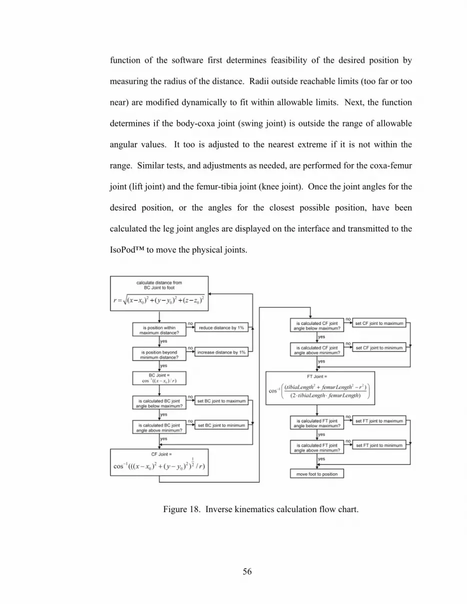
needed to achieve the desired foot position (Fig. 18). The inverse kinematics
56
function of the software first determines feasibility of the desired position by
measuring the radius of the distance. Radii outside reachable limits (too far or too
near) are modified dynamically to fit within allowable limits. Next, the function
determines if the body-coxa joint (swing joint) is outside the range of allowable
angular values. It too is adjusted to the nearest extreme if it is not within the
range. Similar tests, and adjustments as needed, are performed for the coxa-femur
joint (lift joint) and the femur-tibia joint (knee joint). Once the joint angles for the
desired position, or the angles for the closest possible position, have been
calculated the leg joint angles are displayed on the interface and transmitted to the
IsoPod™ to move the physical joints.
Figure 18. Inverse kinematics calculation flow chart.

57
When the individual joints are moved (Func. 1), or the foot position is requested,
the joint position is displayed, allowable joint ranges are updated, leg segment
positions are updated on the interface, and the current foot position x-, y-, and z-
coordinates are calculated and displayed.
Function fwdKin
Description Calculate foot x-, y-, and z-coordinates based on BC, CF, and FT joint angles
Inputs Input As Integer
Outputs z foot z-coordinate x foot x-coordinate y foot y-coordinate
Variables ll effective length from BC joint to foot
Function Body
0
0
0
cos( ) *cos( )sin( ) sin( )
cos( )sin( )
ll femur length CF joint tibia length FT jointz z femur length CF joint tibia length FT jointx x ll BC jointy y ll BC joint
= += + += += +
ii i
ii
Function 1. Forward kinematics equation.
There are also display fields that show the current forces sensed by each foot.
Additionally, the center-of-load icon informs the user of the current load center,
as calculated by summing the force vectors measured by the foot-mounted force
sensitive resistor sensors. Selecting the normalize button resets the base values of
the force sensors, and selecting the React button initiates strafing maneuvers
proportional to and in the direction of external forces acting on the robot.

58
Body Posture
Body height from the ground, pitch about the y-axis, and roll about the x-axis is
achieved through a series of controls on the main screen and is described further
in Section 5.6.
Standing
Two methods of standing are provided: adopting a standing posture, and initiating
the standing cycle. The first method is provided mainly for simulation of drive
characteristics, and is normally not used with the robot connected, as mechanical
problems may arise depending on the current leg joint positions when the Stance
button is selected. Initiating the standing cycle (described further in Section 5.4)
moves leg joints from the Reset position (Fig. 17) into the Stance position through
a series of incremental movements.
Drive Control
Selecting the Drive button displays the Drive Control window (Fig. 17, upper-
left). This window allows the operator to select the desired speed, heading, and
rotation speed.
Moving the speed slider control (Fig. 17, upper-left) sets the desired speed up to a
maximum value of 1.600 (100%), in tenths of an inch per second. The maximum
speed of 0.16in./sec (4.06mm/sec.) was chosen as the fastest speed at which there
are at least four foot positions during the swing phase (four data points along the

59
swing parabola). Faster speeds would distort the swing phase too much and
would jeopardize the walking motions. The maximum speed equates to
9.6in./min. (24.38cm/min.), which is just over one body length per minute.
Setting the speed slider control also initiates a timer which calculates foot
positions and updates actual speed every 100msec. Foot positions are based on
calculations using the Cruse mechanisms (described in detail in Section 5.2 and
Section 5.5). Actual speed is incremented by 0.001 (0.0625%) each 100msec
toward the desired speed; faster if the desired speed is greater than the actual
speed, or slower if the desired speed is lower than the actual speed. The desired
and actual absolute speed values and the desired percentage speed value are
displayed in text fields in the window (Fig. 17, upper-left).
Adjusting the rotation control (Fig. 17, upper-left) sets the desired turning rate
between -1.0 and 1.0, maximum clockwise rotation and maximum counter-
clockwise rotation, respectively. Like the speed control, the rotation control sets
the desired value and initiates a timer. Rotation rate has a maximum value of
1.600 and is incremented toward the desired value each 100msec by 0.001,
similar to the walking speed values.
Selecting the heading dial (Fig. 17, upper-left) changes the direction in which the
robot moves, while facing forward. A heading of 0º is walking forward, 180º is
walking in reverse, and all other directions are considered strafing (see Section
5.5 for additional detail). Unlike setting desired speed and rotation values, new
heading values are implemented immediately. This is accomplished by

60
calculating the position of the new AEP and PEP values (Func. 6) and moving the
foot from its current position along the old path to a similar position along the
new path.
Additional information regarding walking, strafing, and rotating is found in
Section 5.5.
Neck, Head, and Mandible Control
Selecting the Head button from the main screen displays the Head Control
window. This window allows the operator to: adjust pitch, roll, and yaw of the
neck; position the head based on body-centric x-, y-, and z-coordinates; and
actuate the mandibles based on either pincer tip position or desired amount of
gripping force. The operator is also able to view the current force readings for
each of the four mandible force sensors.
5.2 Cruse Controller: Overview, Methodology, and Implementation
In the mid 1970’s Dr. Holk Cruse began research with stick insects to investigate
nervous system feedback mechanisms that control leg movement (Cruse 1976;
Cruse and Storrer 1977). By the mid 1980’s Dr. Cruse and others (Cruse 1985;
Cruse and Müller 1986) were observing leg movements and formulating
mechanisms that cause contralateral and ipsilateral adjacent legs to influence one
another. Fig. 19 describes those mechanisms and shows the influence
connectivity. These interactions between legs adjust the position of the PEP due

61
to the position and status (stance phase or swing phase) of adjacent legs, causing
the stance phase to be elongated or shortened.
Walking/strafing and rotating employ Cruse Mechanisms 1, 2, and 5 (Fig. 19, Fig.
20, Func. 2) to produce varying gaits throughout the range of speeds. It was
determined through previous research (Espenschied et al., 1993) that Mechanisms
3, 4, and 6 were not necessary to create a full range of speed-dependent gaits.
Figure 19. Cruse’s basic rule set for stick insect walking (Schmitz 1998).
For the lengths of the leg segments and in the interest of not allowing the legs to
interfere with one another while walking, a 3in. (7.62cm) step length is used.
This is the initial length; with the AEP 1.5in. (3.81cm) from the center of the
stance toward the direction of travel, and the PEP beginning at 1.5in. (3.81cm)

62
from the center away from the direction of travel. Throughout the walking cycle,
the PEP is adjusted by the position and status (swing phase or stance phase) of the
adjacent feet (Func. 2).
Normally, with pitch and roll values set to zero, the walking height is set to -2.8in.
(-7.11cm) (2.8in./7.11cm below the BC joint), which gives 2.0in. (5.08cm) of
ground clearance. The feet remain at this height throughout the stance phase of
the walking cycle. Once each PEP is reached, a parabolic path is calculated with
an apex height of 0.5in. (12.70mm) for each foot to move through during the
swing phase (Fig. 20, left). This path is updated as the PEP is adjusted due to
affects by the adjacent feet, and each foot position is moved to the closest point
along the new path.
Figure 20. Foot path and signal forms for Mechanisms 1, 2, and 5 with respect to
leg position.

63
Each 100msec, a series of calculations is performed. The first adjusts the actual
speed. Actual speed is adjusted in the direction of desired speed from the current
speed by 0.001 (0.0625% of maximum speed) if not already at the desired speed.
This adjustment occurs both for the walking/strafing speed and the rotation speed.
Next, the base AEP and PEP are set for each foot based on the heading and
current rotation speed values (Func. 6). These values are positioned 1.5in.
(3.81cm) in the direction of foot travel during swing and 1.5in. (3.81cm) in the
direction of foot travel during stance, respectively, to complete the 3.0in.
(7.62cm) step length.
Once the base AEP and PEP are set, the adjusted PEP (PEPa) is determined. The
PEPa is calculated based on the Cruse weights and biases. There are six
mechanism weights and six biases used to calculate the effect of the Cruse
mechanisms on adjacent legs. The six mechanism weights are ipsilateral and
contralateral values for each of the three mechanisms (2, 3, and 5), and the six
biases determine the mechanism influences for each of the six legs. For the front
right foot, PEPa for x- and y-coordinates are calculated below (Func. 2).
Function setPEPa (partial)
Description Adjust PEP values based on mechanism influences of adjacent feet
Inputs none
Outputs PEPa0,x adjusted x-coordinate of leg 0 PEP PEPa0,y adjusted y-coordinate of leg 0 PEP
Variables PEP0,x base x-coordinate of leg 0 PEP PEP0,y base y-coordinate of leg 0 PEP m12 Mechanism 1 value for leg 2 m22 Mechanism 2 value for leg 2 m21 Mechanism 2 value for leg 1 m51 Mechanism 5 value for leg 1 w1i ipsilateral weight for Mechanism 1

64
w2i ipsilateral weight for Mechanism 2 w2c contralateral weight for Mechanism 2 w5c contralateral weight for Mechanism 5 bias2 mechanism weight bias value for leg 2 bias1 mechanism weight bias value for leg 1
Function Body
0, 0, 2 2 2 2
1 1 1 1
0
0, 0, 2 2 2 2
1 1 1 1
0
( 1 1 2 22 2 5 5 )
cos( )( 1 1 2 2
2 2 5 5 )sin( )
x x i i
c c
y y i i
c c
PEPa PEP m w bias m w biasm w bias m w bias
leg headingPEPa PEP m w bias m w bias
m w bias m w biasleg heading
= + +
+ +
= + +
+ +
i i i ii i i i
ii i i ii i i i
i
Function 2. PEP adjustment function segment for leg 0 (front right leg).
In Func. 2, the PEP for leg 0 (front right leg) is affected by Mechanism 2 and
Mechanism 5 from leg 1 (front left leg) and Mechanism 1 and Mechanism 2 from
leg 2 (middle right leg). Each leg has mechanism values based on their status
(swing phase or stance phase) and bias values that are unique to each leg.
Positive x values move more toward the front of the robot; positive y values move
more toward the left side of the robot.
Once the PEPa value is determined the leg status is modified, as needed. If the
foot is at or beyond the PEPa in the direction of movement during the stance
phase, the status is changed to swing. Likewise, if the foot is at or beyond the
AEP in the direction of movement during the swing phase, the status is changed
to stance. If a change of state for a given foot occurs, a counter that holds the
number of calculation cycles in the current state for that foot is reset, otherwise
the counter is incremented. As there is a possibility for each foot to change status,
thus affecting the foot mechanism values, the PEPa values are then recalculated
for each leg.

65
After the status for each foot is determined, its counter is consulted for the
number of 100msec cycles that foot has been in its current state. This counter
aids in determining Mechanism 1 and Mechanism 2 values, as there is a 60msec
interval relative to the shift of state from stance to swing for each. It is also used
in determining where each foot should be on its respective path, either in stance or
swing. Each expected foot position is calculated based on its status, direction of
movement, and time spent in moving in that direction. Each foot is then adjusted
to the calculated position along the path.
As a result of adjusting the PEP for each foot, it is possible to move beyond the
base PEP. When this occurs, the value of Mechanism 5 for that foot increases
linearly beyond 1.0.
5.3 Determining Cruse Mechanism Weights and Bias Values
During early development of the six-legged control software (see Section 6.4) the
Cruse controller was a separate entity that generated x-, y-, and z-coordinates for
the feet and saved them in an electronic file. The file was then imported into the
initial six-legged control interface to make the legs move. Mechanism weights
were generated iteratively through experimentation by hand and produced gaits
that had several situations where adjacent legs were in swing at the same time,
creating an unstable platform. The additional drawback was that movements were
not dynamic, since they were created by another piece of software.

66
When the current six-legged control interface was developed, the Cruse controller
was migrated into the software. This meant dynamic control of the robot, but also
required a slightly modified implementation of the leg interaction algorithms, and
new mechanism weights and leg biases.
Rather than generate mechanism weights through manual experimentation,
evaluation software was created to measure the quality of the gait created by the
Cruse values. This software generated mechanism weights and leg bias values
(Func. 3) and imported those values into a modified version of the six-legged
control interface that exported stance and swing phase conditions for each foot at
each calculation interval (100msec).
The control interface was also modified to automatically set the desired speed to
maximum and terminate itself when that speed was reached. Later updates to the
control interface waited until the maximum speed was reached, then set the
desired speed to zero and terminated once the legs had come to a stop, providing a
cycle from stop to full speed and back to stop.
Function runTest (partial)
Description Set and adjust weight and bias values to be used for evaluation
Inputs none
Outputs weight0 – weight5 current experimental mechanism weights bias0 – bias5 current experimental leg bias values
Variables wAmount weight adjustment amount MAXWEIGHT maximum allowable weight value ( = 1.5 ) random random number generator from 0 to 1 bAmount bias adjustment amount MAXBIAS maximum allowable bias value ( = 1.25 )

67
Function Body
0 5( ) 2 ( / 2)
( ) ( )( ) 0 ( )
( ) ( )( ) ( ) ( )
( ) 2
jwAmount j MAXWEIGHT random MAXWEIGHTweight j MAXWEIGHT random wAmount jif weight j or weight j MAXWEIGHT then
wAmount j wAmount jweight j weight j wAmount j
bAmount j MAXBIAS rand
= →= −
= +< >
= −= +
=
i ii
i i ( / 2)( ) ( )
( ) 0 ( )( ) ( )
( ) ( ) ( )
om MAXBIASbias j MAXBIAS random bAmount jif bias j or bias j MAXBIAS then
bAmount j bAmount jbias j bias j bAmount j
−= +< >
= −= +
i
Function 3. Function to set mechanism weights and bias values for evaluation.
The foot stance/swing status file was then interpreted and evaluated. A score was
generated where negative points were allotted for adjacent legs being in swing
simultaneously, and positive points were assigned when five or more legs were in
stance, or when an alternating tripod gait was achieved (based on speed).
As the scores grew higher, mechanism weights and bias adjustment values were
added to the current values. When a score was lower than the previous, the
adjustment amounts were halved and subtracted from the current values. This
was performed to find local maxima (Func. 4). When a score was identical for
two iterations, the initial mechanism weights and bias values were chosen again
randomly, and the evaluation cycle repeated.
Function runTest (partial)
Description Adjust weight and bias values by adjustment amounts to find local maxima. Change the sign and magnitude of adjustment values if a local maxima is passed to return toward it.
Inputs none
Outputs weight0 – weight5 current experimental mechanism weights bias0 – bias5 current experimental leg bias values

68
Variables lastScore score for the previous set of weights and biases score score for the current set of weights and biases wAmount weight adjustment amount MAXWEIGHT maximum allowable weight value ( = 1.5 ) bAmount bias adjustment amount MAXBIAS maximum allowable bias value ( = 1.25 )
Function Body ' ,
0 5( ) / 2
( ) ( ) / 20 5
( ) ( ) ( )( ) 0 ( )
if lastScore score thenprevious score was better than the current so negateand halve the adjustment amountsj
wAmount j wAmountwBias j wBias j
jweight j weight j wAmount jif weight j or weight j
>
= →= −
= −= →
= +<
( ) ( )( ) ( ) ( )
( ) ( ) ( )( ) 0 ( )
( ) ( )( ) ( ) ( )
MAXWEIGHT thenwAmount j wAmount jweight j weight j wAmount j
bias j bias j bAmount jif bias j or bias j MAXBIAS then
bAmount j bAmount jbias j bias j bAmount j
>= −
= += +< >
= −= +
Function 4. Function to adjust mechanism weights and bias values for evaluation.
The software was run nearly continuously on three to eight computers for a period
of over five months. During this period, many iterations of the evaluation
software were developed in order to refine the fitness functions and methods for
selecting the mechanism weight and bias value initial settings and increment
values. The most recent iteration initializes the mechanism weight and bias
values to a random point within the acceptable range (0 – 1.5 for mechanism
weights and 0 – 1.25 for bias values), and then randomly selects an adjustment
value within twice that range (±1.5 for mechanism weights and ±1.25 for bias
values). As each score increases the adjustment value is added to the current
weight or bias. If the current score is lower than the previous, the adjustment

69
values are halved and multiplied by -1, then added to the current weights and
biases. As with previous versions, when two identical scores are calculated in
sequence the process begins again with random initial and adjustment values.
In addition to alterations in the weight and bias value generation, the fitness
evaluations also changed. In the current version, 100 points are subtracted from
the score for adjacent legs being in swing simultaneously. Twenty points are
added if five or more legs are in stance simultaneously and the speed is less 50%
of maximum. Twenty points are subtracted if the feet are in an alternating tripod
gait at this time, or less than four legs are in stance. The four-legs-in-stance
condition is not penalized as this may represent a quadruped gait and is expected
when migrating from a wave gait to an alternating tripod. Above 50% maximum
speed, 20 points are added for alternating tripod gaits and subtracted if other than
three legs are in stance at the same time, with the exception of all six legs in
stance. The highest achieved score was 36,640 out of a possible 64,000.
The following (Func. 5) is an excerpt from the score calculating function.
CSCORE and ISCORE are the contralateral and ipsilateral penalties for adjacent
legs off the ground, respectively, and are each set to -100. TSCORE and SSCORE
are the tripod and stance rewards, respectively, and are each set to 20.
Function calcScore (partial)
Description Read file with swing/stance state values and assign scores to the set of weight and bias values based on the desired and undesired traits that are observed.
Inputs weight0 – weight5 current experimental mechanism weights bias0 – bias5 current experimental leg bias values
Outputs score score for the current set of weights and biases

70
Variables leg leg number, 0 – 5 starting with the front right leg contacts array of binary values for each leg (1 = swing phase) CSCORE penalty for contralateral adjacent legs in swing phase ISCORE penalty for ipsilateral adjacent legs in swing phase speed speed value for the examined set of contact values SPEEDLIMIT speed above which the gait should be alternating tripod TSCORE reward for being in an alternating tripod gait SSCORE reward for being in wave gait or 6-legged stance
Function Body
:0 5
for all sets of contact values read from filej
if contralateral adjacent legs in swing phase thenscore score CSCORE
if ipsilateral adjacent legs in swing phase thenscore score ISCORE
if speed SPEEDLIMITif gait is alternating
= →
= +
= +<
5 6
3
4 5
tripod thenscore score TSCORE
if or legs in stance phase thenscore score SSCORE
if or fewer legs in stance phase thenscore score SSCORE
if speed SPEEDLIMITif gait is alternating tripod then
score score TSCOREif or legs in
= −
= +
= −>=
= +
2
stance phase thenscore score SSCORE
if or fewer legs in stance phase thenscore score SSCORE
= −
= −
Function 5. Assign scores to the current set of weight and bias values.
Several iterations of the evaluation function were tested with this configuration by
adjusting the speed setpoint at which the transition to an alternating tripod was
desired. Since there does not appear to be a fixed value at which the alternating
tripod gait is initiated in insects, values of 50% and 81% of maximum speed were
tested without biological justification.

71
5.4 Standing
Taking advantage of the approximately 60% efficient, four-stage servo motor
transmissions (stage ratios: 62:10, 50:10, 35:10, and 33:11 for a total of 325.5:1
step-down ratio), the standing cycle begins with the robot body on the ground and
incrementally moves each foot inward toward the body and downward (Fig. 21).
This allows five legs to support the weight of the robot and any payload while
single legs iteratively raise the body.
At the beginning of the standing cycle, the body is resting on the ground and the
six feet are slightly off the ground (0.8in./2.03cm). The front legs are splayed 40º
outward from the medial plane and the rear legs are splayed outward by 35º (Fig.
17). The middle legs are perpendicular to the longitudinal plane. This is different
from the normal positioning of the legs and is used to evenly distribute the legs
about the body and allows each leg to have an opposing counterpart to aid in
lifting and supporting the body.
A cyclic saw-tooth motion is used where each leg first moves inward toward the
body by 0.44in. (1.12cm) and upward by 1.0in. (2.54cm), one at a time (Fig. 21).
The inward distance was chosen as 20% of the distance between the starting and
ending positions, allowing the standing cycle to be completed in five iterations.
Having an upward movement reduces the likelihood that the foot is impeded by
the ground while moving inward. Then, the foot moves in a direct downward
motion by 1.72in. (4.37cm). This lowers each foot by 0.72in. (1.83cm) from the
starting position of the previous cycle.

72
After five iterations, the feet are resting in the standing positions 2.8in. (7.11cm)
below the BC joint (2.0in./5.08cm below the bottom of the robot). This was
selected as being an acceptable amount of ground clearance while minimizing the
torque on the CF joints.
Figure 21. Leg motion during a standing cycle.
5.5 Movement: Walking, Strafing, and Rotating
Initially, when a forward speed is set (Fig. 22), all six legs begin moving rearward
from the neutral position (Fig. 24, left), where each foot starts at points midway
between their respective AEP and PEP. The mechanism weights and bias weights
for each foot modify the PEPs of adjacent feet as defined by the Cruse model
(Fig. 19). During each calculation phase (every 100msec) the PEP values are

73
adjusted based on the position and status (swing phase or stance phase) of each
leg (Fig. 20, right).
Figure 22. Drive cycle flow chart.
As the speed increases (Fig. 23), the gait naturally migrates from a wave gait,
where one leg is off the ground at a time, to a quadruped gait. In the quadruped
gait, two diagonal pairs of legs move at the same time (i.e. right rear and left
middle, and right middle and left front) while the remaining two legs move
independently of the others. This makes the robot appear to have only four legs.
When speed increases further, the quadruped gait shifts which legs are paired

74
together (i.e. right middle and left rear, and right front and left middle). Finally,
the gait moves into an alternating tripod, where the front and rear legs of one side
and the middle leg of the opposite side move together. This moves through a
repeating cycle of one tripod on the ground, all six legs on the ground, then the
other tripod on the ground.
Figure 23. Foot state (swing/stance) as speed increases.
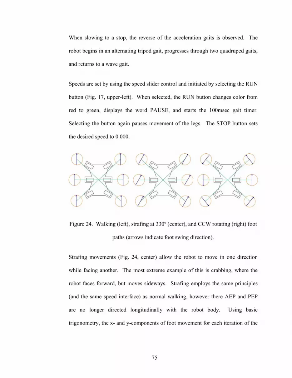
75
When slowing to a stop, the reverse of the acceleration gaits is observed. The
robot begins in an alternating tripod gait, progresses through two quadruped gaits,
and returns to a wave gait.
Speeds are set by using the speed slider control and initiated by selecting the RUN
button (Fig. 17, upper-left). When selected, the RUN button changes color from
red to green, displays the word PAUSE, and starts the 100msec gait timer.
Selecting the button again pauses movement of the legs. The STOP button sets
the desired speed to 0.000.
Figure 24. Walking (left), strafing at 330º (center), and CCW rotating (right) foot
paths (arrows indicate foot swing direction).
Strafing movements (Fig. 24, center) allow the robot to move in one direction
while facing another. The most extreme example of this is crabbing, where the
robot faces forward, but moves sideways. Strafing employs the same principles
(and the same speed interface) as normal walking, however there AEP and PEP
are no longer directed longitudinally with the robot body. Using basic
trigonometry, the x- and y-components of foot movement for each iteration of the

76
walking cycle are determined based on the strafing angle. Walking is considered
as strafing with a heading of 0º (forward).
Selecting the Rev button reverses the heading and double-clicking on the Heading
control resets the heading to 0º (Fig. 17, upper-left).
Rotation adds an additional layer of complexity to the movements. The fastest the
robot can turn is when feet move tangentially to the body centroid at speeds
relative to their distance to the center of rotation (Fig. 24, right). This is when the
middle legs move longitudinally with the body in opposite directions at maximum
speed and the front and rear legs move at a tangent to the body centroid at a
proportionally slower speed, since they are further from the point of rotation. As
slower rotational speeds are desired, the relative speeds of the feet are slowed.
Double-clicking on the Rotation control resets the rotation rate to zero.
Combining walking/strafing, and turning uses vector addition. Each foot path and
speed is determined by the movement speed and rotation speed values
independently. Rotation base speeds are modified relative to the distance from
the foot to the center of the robot as compared to the shortest foot-centroid
distance, which happens to be the middle legs. The x- and y-components for each
method of movement are calculated individually then added, resulting in heading
angles for each leg. New AEP and base PEP values are placed along each leg
path and are separated by the base 3in. (7.62cm) step length (Func. 6).

77
Function setAEPPEP
Description Calculate the AEP and base PEP for the current heading and amount of rotation, then move each foot incrementally toward the PEP (in stance phase) or the AEP (in swing phase).
Inputs none
Outputs AEPi,x new AEP x-coordinate for the current leg AEPi,y new AEP y-coordinate for the current leg PEPi,x new base PEP x-coordinate for the current leg PEPi,y new base PEP y-coordinate for the current leg
Variables deltai,x amount of leg movement along the x-axis for this cycle deltai,y amount of leg movement along the y-axis for this cycle dSpeed current walking/strafing speed angle body heading (strafing angle) tSpeed current amount of rotation legturni,x x-coordinate distance from the foot to robot center legturni,y y-coordinate distance from the foot to robot center leganglei individual leg heading measured from PEP to AEP STEPLENGTH nominal step length ( = 3.0in. ) centeri,x x-coordinate center of the foot path centeri,y y-coordinate center of the foot path
Function Body , ,
, ,
, ,
, ,
, ,
0 5cos( )sin( )
arctan( / )
cos( )si
i x i x
i y i y
i i y i x
i x i x i
i y i y
idelta dSpeed angle tSpeed legturndelta dSpeed angle tSpeed legturn
legangle delta delta
AEP center STEPLENGTH legangleAEP center STEPLENGTH
= →= +
= +
=
= +
= +
i ii i
ii
, ,
, ,
n( )
cos( )sin( )
i
i x i x i
i y i y i
legangle
PEP center STEPLENGTH leganglePEP center STEPLENGTH legangle
= −
= −
ii
Function 6. Calculate individual foot headings and assign new AEP and base PEP
coordinate values.
Each leg is maneuvered individually throughout the stance and swing cycles with
its own heading to produce the composite effect of combing the desired
walking/strafing and turning elements.
As the robot heading is changed during adjustments in walking/strafing and/or
turning, the base AEP and PEP values for each foot are updated each 100msec

78
cycle. The feet are dynamically moved from their positions along the old foot
headings to similar positions along the path for the new foot headings.
5.6 Body Posture: Height, Pitch, and Roll
The main screen of the software interface (Fig. 17) has three controls to adjust
ground clearance (body height), body pitch and body roll.
Ground clearance can be set from -0.1in. (-0.25cm) to -3.5in. (-8.89cm). The
negative values are used to represent the distance that the ground is, relative to the
BC joint. Adjusting the Ground slider control moves the z-coordinate value for
all legs. This value may be clamped high at -0.1in. (-0.25cm) or low at -3.5in.
(-8.89cm), depending on the settings of the Pitch and Roll controls.
Body Pitch is set by a rotary control and adjusts the robot about the y-axis and is
selectable up to ±15.0º. Positive pitch values raise the front of the robot, while
negative values raise the rear. Pitch is adjusted by equally moving the heights of
the front and rear pairs of legs in opposite directions up to ±6.0º. At +6.0º the
front legs are at their lowest point. From +6.0º to +15.0º, the middle and rear legs
are raised proportionately to achieve the desired pitch. For negative pitches
beyond -6.0º, the middle and front legs are raised proportionately. Double-
clicking on the Pitch control resets pitch to 0.0º.
Another rotary control is used for the Body Roll setting, which adjusts the robot
about the x-axis. Adjustments equally lower the leg heights on one side of the
robot and raise the leg heights on the other side, depending on the selected roll

79
value. Positive values raise the right side of the robot, and negative values raise
the left side. Roll values can be set up to ±15.0º. Double-clicking on the Roll
control resets body roll to 0.0º.
The combined absolute values of adjustment of pitch and roll cannot exceed 15º.
As one control advances such that the combined absolute values go beyond 15º,
the other control is reduced proportionately. For example, raising pitch by one
degree with values of +11º pitch and -4º roll will result in +12º pitch and -3º roll.
As a value is adjusted so that the combination of absolute values is below 15º, the
other control is not affected. For example, lowering pitch by one degree with
values of +12º pitch and -3º roll will result in +11º pitch and -3º roll.
5.7 Force Feedback Sensors and the Affects on Movement and Posture
The environment is sensed through force transducers in the feet and at the ends of
the mandible pincers, and through current sensors attached to the power supply
wires of the neck servo motors. These sensors direct movements of the neck and
legs.
While holding an object, the neck measures the weight of the object through
vertical forces acting on the pincer sensors and changes in the neck lift servo
motor current, and then sets the values as a new baseline. These values are
measured and recorded on the BrainStem modules located in the head via the
ADC inputs. As the force sensed in the mandibles and the neck changes, the neck
moves to return mandible sensor values to the baseline. When the neck nears the

80
end of its range of motion in a particular direction, signals are passed from the
BrainStem modules to the System Controller. The System Controller initiates
walking/strafing and rotation movements to compensate. This, in turn, alters the
forces sensed in the mandibles and neck and causes adjustments within the neck
to return toward the centers of the ranges of motion. They cycle repeats until the
neck and legs are in neutral positions.
The mandible and neck sensors are best suited for forces acting laterally and
vertically, but not longitudinally. For longitudinal forces, the foot sensors are
used. As forces act along the centerline of the robot, rearward forces will cause
the rear foot sensors to register higher loads while the front foot sensors will
register lower loads, due to the elevated position of the head relative to the feet.
When this occurs, the System Controller initiates walking in the direction of, and
proportional to, the perturbation, thereby minimizing the force (Func. 7). When
the foot sensor values return to baseline values, walking is stopped.
Function findForceCenter
Description Based on the foot-mounted force sensor values, calculate the center of force.
Inputs footForce0 – footForce5 foot-mounted force sensor values
Outputs speed speed at which to move along the external force vector angle direction of the external force vector
Variables forceCenterx x-coordinate of the force center from the body center forceCentery y-coordinate of the force center from the body center xValueleg x-coordinate current leg’s foot position yValueleg y-coordinate current leg’s foot position bodyReact flag for active compliance behavior status maxSpeed maximum walking/strafing speed

81
Function Body (( )
(( )
arctan(
x leg leglegs
y leg leglegs
for all legs whose footForce FORCETHRESHOLDforceCenter footForce FORCETHRESHOLD xValue
forceCenter footForce FORCETHRESHOLD yValue
if bodyReact is True thenangle forceCente
>=
= −
= −
=
∑
∑
i
i
/ )y xr forceCenter
speed forcevector maxSpeedif speed maxSpeed then
speed maxSpeed
=
>=
i
Function 7. Calculate external force magnitude and direction, and move in the
direction of the force vector, relative to the body center.
Similarly, perturbations directly to the robot body cause shifts in the center of
load as measured by the foot force sensors. As with external forces sensed while
carrying objects, body perturbations cause walking/strafing in the direction of,
and proportional to, the sensed force (Func. 7). When the foot sensors indicate
the perturbation has stopped, robot movement is also stopped.
5.8 Control and Autonomy
Currently, the robot is power autonomous and control tethered. While the control
link may be made wireless in the next stage of development, the System
Controller will remain an external computer until additional testing and
development can solidify the system parameters. At such time, the BrainStem
modules will connect to the IsoPod™ directly, and the IsoPod™ will gather
sensor data and initiate body movements autonomously.

82
Having an external System Controller aids in development by providing an easily
changeable software platform, and a graphical user interface. These features
allow new software behaviors and functionality to be added and updated more
simply, and provide virtual visual feedback on performance without the need for
the robot to be connected.
Once the software features have been finalized and fully tested, leg control and
behavior functionality currently on the external System Controller will be
programmed onto the IsoPod™ and BrainStem modules, providing the robot with
control autonomy.
Future developments will include an attached abdomen to house a PDA, which
will provide system goals and path planning.

83
CHAPTER VI
PROJECT DEVELOPMENT AND EVOLUTION
6.0 General
Many incremental steps were taken during the development of the BILL-Ant-p
project. Setting intermediate goals within the framework of the entire project
allowed progress to be better evaluated and managed. This becomes more
important when component integration is being performed and when new
methods and practices are being tested or implemented.
6.1 One-Leg Test Rig
After examining the attributes of the Lynxmotion, Inc. Hexapod 3 robot it was
decided to construct a single prototype leg to test the strength and lifting capacity
of two mini-size servo motors (similar to those that are included with the kit). A
pair of Hitec HS-81MG servos (the original servo motors that were offered with
the Lynxmotion, Inc hexapod kit) and a pair of Hitec HS-225MG servos (Hitec
RCD, Inc., Poway, CA, USA) were fitted into a custom-made polycarbonate leg
(Fig. 25).
The leg had a mounting plate, which housed the lift joint servo motor and was
constructed by separating two 0.125in. (3.18mm) thick pieces of 2.25in. (5.72cm)
long polycarbonate material with 0.25in. (6.35mm) spacers. The tibia was created
similarly with another pair of polycarbonate plates that were 5.0in. (12.7cm) long

84
and housed the knee joint servo. The lift joint and knee joint servo motors were
connected by a pair of 0.125in. (3.18mm) thick, 2.25in. (5.72cm) long pieces of
polycarbonate that were separated by 1.5in. (3.81cm) spacers and formed the
femur. One femur plate was mounted to the output horns of the lift and knee
servos, while the other plate was supported by plastic axles attached by double-
sided adhesive tape to the underside of each motor. The two plates were held
together by steel screws and nylon sleeves.
Figure 25. One-leg test rig.
Testing the Hitec HS-81MG motors (41.66oz.-in. / 3.01kg-cm torque, 0.09s/60º
speed) showed that they would be insufficient to lift a 5lb. (2.72kg) robot with
only two legs. The ability of two legs to support the weight of the entire robot

85
was an early goal of the system, as it was desired to have one robot safely carry
itself and the weight of another robot as cargo.
The slightly larger Hitec HS-225MG motors (66.7oz.-in. / 4.81kg-cm torque,
0.11s/60º speed) performed better, but were still not enough to lift the desired
weight, for the tested lengths of the leg segments.
Two options remained: shorten the leg segments so that more force could be
applied, or find better servo motors. As ground clearance was desired to be
approximately 2.0in. (5.08cm), shorter leg segments were not an option.
After researching power/weight ratios, sizes, and costs of various servo motors,
the MPI MX-450HP servos (Maxx Products, Inc., Lake Zurich, IL, USA) were
purchased. These motors are standard-size servos with 116 oz.-in. (8.37kg-cm) of
torque and can rotate through a 60º arc in 0.18sec. They are half as fast as the
Hitec HS-81MG servos, but nearly three times the torque at 2.5 times the weight.
6.2 Basic IsoPod™ Interfacing
While the servo motors were being researched and tested, a servo controller was
researched. The Lynxmotion, Inc. (Pekin, IL, USA) Hexapod 3 kit recommended
using a New Micros, Inc. (Dallas, TX, USA) IsoPod™ servo controller. With an
attached daughter board, it could support up to 26 R/C servo motors, was powered
by 3.3vdc/5.0vdc, offered two RS-232 serial ports, was programmable, and had
eight 12-bit ADC inputs. Although the controller was deficient in the number of
desired ADC inputs (at least 18 are needed to read values from each joint motor),

86
the other features were more than adequate. The board was ordered and interface
testing began.
It was decided, in the interest of time, to begin with a host computer sending
commands to the IsoPod™. Programming the controller for autonomous use is
scheduled for a later date. The IsoPod™ is capable of interpreting proprietary
ASCII command sent via the serial port to perform tasks or retrieve ADC data
values.
For testing, Microsoft HyperTerminal (Microsoft Inc., Redmond, WA, USA) was
used to alter the IsoPod™ baud rate, toggle on-board LED indicators, and retrieve
ADC values. After discovering example values for controlling R/C servo motors
in the user guide (New Micros, Inc. 2003), a simple program was written in
Visual Basic 6.0 to actuate a series of three servos. The program was then
expanded to control six servos (two 3-DOF legs).
6.3 Two-Leg Test Platform and Software Interface
Once successful interfacing was achieved with the IsoPod™ microcontroller, two
new prototype legs, constructed of 6061 aluminum and carbon fiber were made.
The two-legged test platform (Fig. 26) had 0.125in. (3.18mm) thick 6061
aluminum tibiae that held the knee joint servo motors and were 4.25in. (10.80cm)
from the motor axle to the tip of the foot. Femurs were constructed from two
parallel 0.0625in. (1.59mm) thick carbon fiber plates separated by a 1.81in.
(4.60cm) aluminum strut, and were 2.25in. (5.72cm) from the lift joint motor axle

87
to the knee joint motor axle. The length was chosen as being the shortest length
that allowed free movement of the servo motors.
Figure 26. Two-legged test platform with the attached stand.
Aluminum housings were created for the lift joint servos, so that the swing joint
servos could be attached. Each joint used the internal dual ball-bearing supported
output shaft of the servo motor as one axle and had a 0.25in. (6.35mm) diameter
threaded sleeve mounted on the opposite side of the joint as a second axle, for
additional support. The swing joint motors were mounted inverted into a carbon
fiber plate, and the lift joint motor housings axles were secured through holes in a
parallel carbon fiber plate. The two plates were separated and supported by a

88
0.1875in. (4.76mm) thick, 1.80in. (4.57cm) tall 6061 aluminum spine. The spine
was then secured to a vertical stand with mounted wheels for mobile testing.
The six servo motors were connected to the IsoPod™, which was suspended from
the stand. Power was originally supplied by a dual-output bench power supply
with a combined maximum output of approximately 5.0A. There were no issues
when the servo motors were actuated individually. However, when all six servos
were operated simultaneously, the power supply breaker tripped repeatedly,
indicating the motors were drawing more current than could be supplied. As a
result, power was then supplied by two HydriMax Ultra 4.8vdc 2000mAH NiMH
batteries (Hobbico, Inc., Champaign, IL, USA). One was used for IsoPod™ logic
power and a second powered the servo motors. Although the batteries were only
4.8vdc (as opposed to 6.0vdc), they were readily available and provided enough
steady-state and peak current to run all six servo motors.
A new interface was created in Visual Basic to control the two legs and perform a
series of experiments (Fig. 27). The interface allowed the operator to manipulate
each of the six joints manually, and some basic leg patterns were created to
simulate walking for the front legs of a cockroach. Foot path data was taken from
observed cockroaches while walking (Boggess et al. 2004). The two buttons on
the interface: Swim and Walk performed the walking motions for each leg in-
phase, and 180º out-of-phase, respectively.

89
Figure 27. Two-legged test platform user interface.
Once control of leg movements was possible, feedback was desired. The main
controller blindly issues a command while the servo motor controls itself to
accommodate the command; no feedback information is received by the main
controller. Having this information would make things such as velocity control
possible. Each of the six servo motors uses a potentiometer coupled to the output
shaft to determine its position. This value is measured by the internal servo
control board that sets direction and speed of the dc motor. So, signal wires were
connected to the electronic output of the potentiometers and fed into the ADC
inputs on the IsoPod™. Without amplification, the signals varied by 0.82vdc

90
over a 90º range of motion and were displayed on the user interface (Fig. 27).
Using amplification and a dc offset, this could be useful position feedback for the
main controller. However, since the IsoPod™ only has eight ADC inputs, and
another ADC input board that could be integrated onto the platform was not
found, research into this area stopped.
Next, a basic standing routine was created to see if the legs had sufficient power
to lift themselves off the ground. It became difficult to test with only two legs,
since moving the legs inward and downward simultaneously on a high-friction
surface (low-pile carpeting) was impossible due to the feet snagging on the carpet,
and there was no way to easily lift one leg while the other remained on the ground
without the stand becoming unstable and toppling. It was time to create a six-
legged platform.
6.4 Initial Six-Leg Platform and Software Interface
The six-legged interface (Fig. 28) was created from the ground up, but used
elements such as the IsoPod™ communication function and the forward
kinematics equations that were developed in the two-legged interface software.
New features in this interface included a stand-up routine, inverse kinematics for
user-determined foot placement, and the ability to import pre-generated foot
position patterns, which were created by an external software application that
used a Cruse control model.

91
Figure 28. Initial six-legged test platform user interface.
An application written in the C programming language used a Cruse model for leg
coordination and generated two-dimensional foot paths in the x- and z-plane for
all six legs. The path values were saved in an ASCII text file with a fixed y-
dimension value for each leg. Selecting the Cruse button on the six-legged
interface read the file and, using a timer to set the movement rate, entered the (x,
y, z) values into the on-screen fields and moved the leg joint using inverse
kinematics equations. The result was a canned walking routine that demonstrated
the interface was correctly calculating joint values and displaying a continuously
varying series of stable gaits.
As development on the interface software progressed, the designed and machined
final parts for the robot body and legs were made. When assembled and powered

92
by three HydriMax 4.8vdc NiMH batteries (one for IsoPod™ logic power and
two in parallel for servo power), joint calibration was performed.
Since R/C servo motors use an internal potentiometer for position feedback, all
positions are absolute (as opposed to using a shaft encoder, where the positions
are relative to a starting location) and need to be calibrated by orienting the
splined output horn with a known position. To perform this operation, the
software interface sent servo positions to the IsoPod™, which moved the
associated servos. The leg segments were then removed and reattached in the
orientation commanded by the interface. This was the first time the current BILL-
Ant-p body parts were assembled and powered with a control interface; it went
successfully.
Once the calibration was completed, a test of the stand-up routine was performed.
It was uncertain if the robot would be able to successfully lift itself with only two
4.8vdc batteries supplying servo power, since the design called for three 6.0vdc
batteries. The test completed without incident, even with the fewer and lower
voltage batteries.
Due to the successful results of the standing test, an initial walking test using the
imported leg positions from the Cruse control software was initiated. This was
also completed successfully and marked the first steps taken by the robot (and on
its first attempt). Several additional walking tests were performed over
subsequent days.

93
Since there was no velocity control to make smooth leg movements, refinements
were made to the order in which leg joints were activated. The motor controller
inside each servo is essentially a speed controller with proportional position
feedback, so greater angular displacements move at proportionally greater speeds.
In an attempt to reduce some of the seemingly erratic leg movements, an
algorithm was established that initiated movement of the servos based on the
angular displacement, where the servo traveling the greatest distance was initiated
first. This was a noticeable improvement to the smoothness of leg movements.
Also during this time, four MPI two-cell 2400mAH 7.2vdc Li-ion batteries and
four MPI ACC134 6-volt Regulators were purchased and installed to supply
power to the IsoPod™ and servo motors (see Section 4.4).
6.5 Current Six-Leg Platform and Software Interface
The next step in software development was to incorporate the Cruse controller
into the robot interface. This interface is described in Chapter V.
6.6 Control and Autonomy
In future revisions of the BILL-Ant-p robot, the Cruse controller, leg
coordination, and active compliance commands provided by the off-board System
Controller will be migrated onto the IsoPod™ and BrainStem microcontrollers.

94
6.7 Prototype Mandibles
A set of prototype mandibles (Fig. 29) was designed to test the feasibility of
implementing single-servo actuated dual pincers. The prototype was heavier than
hoped at 8.31oz. (236g), and only provided approximately 2.5lbs. (1.14kg) of
gripping force at the tips of the pincers. By recalculating hinge point positions
and actuating cable attachment points, a new design emerged that provides
approximately 5.6lbs (2.55kg) of force and weighs 5.17oz. (147g).
Figure 29. Prototype mandibles closed and open as viewed from the bottom.

95
CHAPTER VII
SYSTEM PERFORMANCE
7.0 General
This chapter quantifies the robot component weight characteristics, load
capacities during various tasks, maneuvering performance, active compliance
performance, and battery life.
7.1 System Component Masses
The robot mass, without the neck, head, or mandibles, is 5.10lbs. (2.32kg).
System, subsystem, and component masses were weighed on a scale with 1.0g
resolution. Ounce values were calculated from the gram masses. Both are listed
below in Table 3.
Component or Subsystem
Mass (oz./g)
Body with Legs and Electronics 81.59 / 2318
Body Section 5.81 / 165 Top Plate 1.58 / 45 Bottom Plate 1.58 / 45 Spine 1.62 / 46 Front Plate 0.46 / 13 Rear Plate 0.46 / 13 Fasteners and misc. 0.11 / 3

96
Leg (x6) 8.98 / 255 Coxa 0.77 / 22 Femur 0.63 / 18
Front Plate 0.28 / 8 Rear Plate 0.18 / 5 Yoke Strut 0.18 / 5
Tibia 0.39 / 11 Foot 0.32 / 9 R/C Servo (x3) 2.25 / 64 Fasteners and misc. 0.11 / 3
IsoPod 1.30 / 37 Power System 18.09 / 514
Battery (x4) 3.01 / 94 Power Converter (x4) 0.63 / 18 Switches, Holders, Fuse, Fasteners and misc.
2.32 / 66
Fasteners and misc. 2.53 / 72
Table 3. Component and subsystem masses.
7.2 Lifting and Sustaining Load Capacities
Two sets of experiments were performed for load capacity testing. The first was
lifting a payload from a starting position where the body is resting on the ground
and then moves to a full standing position; the second was sustaining a payload
while in a standing posture. Initial tests were performed on a low-pile carpeted
floor with a fresh set of batteries. It was suspected that the relatively rough
surface provided by the carpet aided in the load lifting and sustaining capacities,
so additional tests were performed on a smooth, laminated surface. Overall the
maximum capacities are reduced when on the smooth surface (shown in Table 4,
Table 5, Table 6, and Table 7), as expected.

97
Also, in the interest of observing some characteristics of performance over
waning battery life, tests were repeated and load capacities were observed over
time. In Table 4, Table 5, Table 6, and Table 7, operation time of the battery
refers to time spent performing the experiments where the robot is active; standby
time is where the robot is inactive, but the batteries are still installed.
Since the servo and logic power busses have switches installed after the voltage
regulators, there is power consumed by the regulators even when the robot is
“off”. This is termed “standby time” in the tables below.
Battery Operation/Standby Time
Prior to Test (minutes/minutes)
Carpet Floor
(lbs./kg)
0 / 0 7.0 / 3.18 15 / 177 6.0 / 2.73 16 / 177 6.0 / 2.73
Table 4. Robot lifting load capacities on carpeted surface.
Battery Operation/Standby Time
Prior to Test (minutes/minutes)
Smooth Surface
(lbs./kg)
4 / 175 5.0 / 2.27 7 / 175 4.0 / 1.82 11 / 176 3.0 / 1.36
Table 5. Robot lifting load capacities on smooth surface.

98
Battery Operation/Standby Time
Prior to Test (minutes/minutes)
Carpet Floor
(lbs./kg)
1 / 0 19.0 / 8.64 11 / 14 15.0 / 6.82 17 / 177 13.0 / 5.91
Table 6. Robot sustaining load capacities on carpeted surface.
Battery Operation/Standby Time
Prior to Test (minutes/minutes)
Smooth Surface
(lbs./kg)
5 / 10 11.0 / 5.00 13 / 175 9.0 / 4.09
Table 7. Robot sustaining load capacities on smooth surface.
7.3 Walking Load Capacity
The robot was able to maintain a speed of 0.16in./sec (4.06mm/sec.) on a carpeted
surface with a 7.0lb. (3.18kg) load on its back for a duration of 0:03:08. This test
was performed after approximately 11min. of weight lifting tests and 14min. of
standby time. After about three minutes of walking with the load, the body
sagged slightly under the weight and then collapsed when the right rear leg
transitioned from stance to swing phase.
Given the observed weight lifting and sustaining performance over the life of the
batteries, it is suspected that the robot would be able to walk for about 30 minutes
with no load, and roughly 15 minutes with a 5.0lb. (2.72kg) payload with a newly
charged set of batteries.

99
7.4 Driving and Turning Performance
A series of performance tests were conducted to verify the ability of the robot to
move at different headings and perform rotation maneuvers at varying speeds.
Similar to forward walking, strafing and rotating uses the Cruse mechanism
weights to migrate through a series of stable gaits (Fig. 23). For strafing, the
direction of the AEP for each leg is set identically so that the robot moves in the
desired direction while facing another (Fig. 24, center). Rotating occurs by
setting the AEP headings tangentially in the direction of rotation (Fig. 24, right).
The continuum of gaits is observed in this mode as well. See Section 5.5 for
additional information on strafing and rotation.
The robot was able to successfully move in all directions while maintaining a
fixed heading. This test was performed in 10º increments over 360º of planar
movement at speeds up to 0.08in/sec.
Turning tests were also performed. During these tests, the robot rotated at a
maximum rate of 1.53º/sec.
7.5 Body Movement in Response to External Forces
Initial testing of the force-reactive behavior was less than impressive. Bench
testing of the foot-mounted sensors and calculation of the load center was
successful. However, placing the robot on the ground yielded mildly erratic and
slow-responding results. It was observed that by mounting the feet solidly to the
ends of the tibiae (Fig. 8) the force sensors were rarely flat on the ground. This

100
caused lower force readings and reduced the responsiveness of the robot to
external forces. Remounting the feet to allow a pivoting motion, like a free-
moving passive ankle, proved worse as the feet were frequently tilted on edge as a
result of moving the legs. Using a spring-damper mechanism in the ankle may
resolve this issue if a passive ankle design is used.
Another approach taken was attaching a 0.5in. (12.7mm) long #4-40 screw to the
bottom plate of each foot. This allowed contact forces to be sensed over a larger
range of tibiae angles with respect to the ground since contact was made with the
screw instead of the foot bottom. Using this method and applying a pushing force
laterally to the robot body at the level of the BC joint servos caused the robot to
respond by retreating from the applied force. Tests were performed by applying
force at several points on the robot.
7.6 Battery Life and Power
Through experimentation with lifting, sustaining, and transporting various
weights, the current draw was approximately 12A. With three 2400mAh Li-Ion
battery packs in parallel, the robot would be able to operate for about 36 minutes
while actively moving and lifting.
Each of the MPI MX-450HP servo motors contains a small dc motor that
consumes 1125mW of power at stall torque. This equates to 20.25W of power for
the 18 servo motors in the legs.

101
CHAPTER VIII
FUTURE WORK
8.0 General
Once the head, neck, and mandibles have been fully integrated into the BILL-Ant-
p robot and tested, several improvements are proposed to enhance the
performance and functionality of the robot. Among these improvements are:
object identification and gathering, path planning, event-based communication,
and cooperative group behaviors.
8.1 On-board Control, Navigation, and Communication
When the robot functionality as an autonomous stand-alone, actively compliant
unit is finalized, its role will be expanded, and it will become an autonomous part
of a community of robots. To achieve this integration, inter-robot communication
will need to be developed, in addition to autonomous navigation and control.
As mentioned in above sections, the next phase of development for the robot is to
have the Cruse control implemented on the IsoPod™ microcontroller and move
all active compliance control on-board the robot (in the IsoPod™ and BrainStem
microcontrollers). This will allow the robot to be both power and control
autonomous as an actively compliant agent. This, however, is not enough to
achieve the goal of object searching, manipulation, and gathering.

102
To advance the functionality of the robot, on-board navigation and object
recognition will be required. These features will allow the robot to autonomously
navigate the terrain in search of meaningful objects for observation and/or
collection. It is proposed that a personal data assistant (PDA) with wireless
communication be added and interfaced with the IsoPod™ to set goals, navigate
the terrain, and decide which observed objects are noteworthy. A vision system
may be added to assist both in object recognition and navigation.
Making the robot part of a group of other robots will require communication.
Based loosely on the leaf-cutter ant’s event-based broadcast communications (see
Section 8.2) the robot will be able to send broadcast messages to other robots
within range when significant events occur, such as “object found”, “returning to
home point”, and “help required”.
8.2 Event-Based Broadcast Communication
Leaf-cutter worker ants employ a form of broadcast communication during
distinct phases while gathering food (Hölldobler and Wilson 1990; Yahya 2000).
These messages are generated by “stridulation”, a process where the ant moves a
ridged section of its abdomen against the hind legs, generating vibrations in the
substrate (Hölldobler and Wilson 1990; Yahya 2000). These vibrations are
capable of being received over short distances and signify events during the
gathering process. The signals are broadcast into the general environment for all
nearby ants, rather than being used as specific ant-to-ant communication.

103
In this vein, the BILL-Ant-p will have the ability to send event-based messages to
all other robots within the range of reception. In order to limit the range, either
Bluetooth communication (up to about 36ft. / 11m), or WiFi communication (up
to about 300ft. / 92m) with a software limitation on the distance from which a
message will be acknowledged will be used.
8.3 Leader and Helper Roles
Initially, all object-seeking and navigating robots adopt the role of Leader. As
Leaders, each robot autonomously navigates the terrain in search of meaningful
objects, gathering those it can by itself. When a robot encounters an object it
cannot retrieve alone, it broadcasts a “request for help” message. Other robots
within range of the broadcast send an acknowledgement of receipt and commence
a bidding process for which robot, if any, will help the one requesting assistance
(see Section 8.4) (Gerkey and Matarić 2002). Once a robot is chosen to help, it
adopts the Helper role and navigates itself to the Leader that requested help.
In its current state as an actively compliant mobile robot, the BILL-Ant-p is
already fulfilling a part of the role as a Helper. Once the Helper arrives at the
object and both the Leader and Helper engage it with their mandibles, the Leader
will return the object to the home point. It is the role of the Helper to maintain a
neutral posture, where legs are evenly placed about the body and the neck servo
motors are centered. To achieve this posture, the Helper will respond to forces
exerted on it by the object it is holding, ultimately generated by the Leader which
is also grasping the object. The Helper will continue to move its neck and legs in

104
response to the external forces until the object is returned to the home point.
Once the object has been returned, the Helper resumes its role as a Leader.
8.4 Helper Role Bidding Process
Part of the events leading to multiple robots manipulating a common object is the
Helper role bidding process (Gerkey and Matarić 2002). This involves multiple
Leader robots vying for the opportunity to become Helpers. The process will be
based on range from the robot that is requesting assistance and current task
priority. Leaders currently engaged in tasks with high priority, such as returning
objects to the home point, will be less likely to become Helpers. Likewise, robots
engaged in similar priority tasks will be more likely to become Helpers if they can
arrive at the help-requesting robot sooner than another robot.

105
LIST OF REFERENCES
(LISTED ALPHABETICALLY BY FIRST AUTHOR AND IN REVERSE CHRONOLOGICAL ORDER)
Angle, C., Design of an Artificial Creature, S. M. Thesis, Department of Electrical
Engineering and Computer Science, MIT, Cambridge, MA, USA, June 1991. Barnes, D. P., “Hexapodal Robot Locomotion Over Uneven Terrain,” in Proc. IEEE
Conf. on Control Applications. Trieste, Italy, pp. 441 – 445, September 1998. Berns, K., “The Walking Machine Catalog: Walking Machine Catalog,” World Wide
Web, http://www.walking-machines.org/, 2005. Boggess, M. J., Schroer, R. T., Quinn, R. D., Ritzmann, R. E., “Mechanized Cockroach
Footpaths Enable Cockroach-like Mobility,” in Proc. IEEE Conf. on Robotics and Automation, Vol. 3, pp. 2871 – 2876, New Orleans, LA, USA, 26 April – 1 May, 2004.
Brooks, R. A., “A Robot That Walks; Emergent Behaviors from a Carefully Evolved
Network” Technical Report, MIT AI Lab Memo 1091, Cambridge, MA, USA February 1989.
Buschmann, A., “Home of Tarry I & II: Design of the Walking Machine Tarry II,” World
Wide Web, http://www.tarry.de, March 2000. Buschmann, A., “Home of Tarry I & II: Frequently Asked Questions about Tarry,”
World Wide Web, http://www.tarry.de, March 2000. Cruse, H., Müller-Wilm, U., Dean, J., “Artificial Neural Nets for Controlling a 6-legged
Walking System,” in Proc. of the Second International Conference on Simulation of Adaptive Behavior: From Animals to Animats 2, MIT Press, Cambridge, MA, pp. 52 – 60, 1993.
Cruse, H., “What Mechanisms Coordinate Leg Movement in Walking Arthropods?”
Trends in Neurosciences, Vol. 13, pp. 15 – 21, 1990. Cruse, H., Müller, U., “Two Coupling Mechanisms which Determine the Coordination of
Ipsilateral Legs in the Walking Crayfish,” J. Exp. Biol., Vol. 121, pp. 349 – 369, 1986.
Cruse, H., “Coactivating Influences between Neighbouring Legs in Walking Insects,” J.
Exp. Biol., Vol. 114, pp. 513 – 519, 1985.

106
Cruse, H., Storrer, J., “Open Loop Analysis of a Feedback Mechanism Controlling the Leg Position in the Stick Insect Carausius morosus: Comparison between Experiment and Simulation,” Biol. Cybern., Vol. 25, pp. 143 – 153, 1977.
Cruse, H., “On the Function of the Legs in the Free Walking Stick Insect Carausius
morosus,” J. Comp. Physiol., Vol. 112, pp. 235 – 262, 1976. Espenschied, K. S., Quinn, R. D., Chiel, H. J., and Beer, R. D., “Biologically Based
Distributed Control and Local Reflexes Improve Rough Terrain Locomotion in a Hexapod Robot,” Robotics and Autonomous Systems, Vol. 18, pp. 59 – 64, 1996.
Espenschied, K. S., Quinn, R. D., Chiel, H. J., and Beer, R. D., “Biologically-Inspired
Hexapod Robot Project: Robot II,” in Video Proc. IEEE International Conference on Robotics and Automation (ICRA ’95), Nagoya Congress Center, Nagoya, Japan, May 21 – 27, 1995. (Won Best Video Award)
Espenschied, K. S. and Quinn, R. D., “Biologically-Inspired Hexapod Robot Design and
Simulation,” in Proc. AIAA Conference on Intelligent Robots in Field, Factory, Service and Space, Houston, Texas, March 20 – 24, 1994.
Espenschied, K. S., Quinn, R. D., Chiel, H. J., and Beer, R. D., “Biologically-Inspired
Hexapod Robot Control,” in Proc. 5th International Symposium on Robotics and Manufacturing: Research, Education and Applications (ISRAM ’94), Vol. 5, pp. 89 – 94, Maui, Hawaii, August 14 – 18, 1994.
Espenschied, K. S., Quinn, R. D., Chiel, H. J., and Beer, R. D., “Leg Coordination
Mechanisms in Stick Insect Applied to Hexapod Robot Locomotion,” Adaptive Behavior, Vol. 1, No. 4, pp. 455 – 468, 1993.
Ferrell, C., “Robust Agent Control of an Autonomous Robot with Many Sensors and
Actuators,” Technical Report, MIT Artificial Intelligence Lab, TR-1443, Cambridge, MA, USA, 1993.
Gaßmann, B., Scholl, K.-U., Berns, K., “Behavior Control of LAURON III for Walking
in Unstructured Terrain,” in Proc. Intl. Conference on Climbing and Walking Robots (CLAWAR ’01), pp. 651 – 658, Karlsruhe, Germany, September 2001.
Gerkey B. P. and Matarić, M. J., “Sold!: Auction Methods for Multirobot Coordination,”
in Proc. IEEE Transactions on Robotics and Automation, Vol. 18, No. 5, 758 – 768, October 2002.
Hölldobler, B., Wilson, E., The Ants, The Belknap Press of Harvard University Press,
Cambridge, Massachusetts, 1990.

107
Matarić, M. J., Nilsson, M., and Simsarian, K. T., “Cooperative Multi-Robot Box-Pushing,” in Proc. IEEE Intl. Conference on Intelligent Robots and Systems, Vol. 3, pp. 556 – 561, Pittsburgh, PA, USA, August 5 – 9, 1995.
Melhuish, C., Holland, O., and Hoddell, S., “Collective Sorting and Segregation in
Robots with Minimal Sensing,” in Pfeifer, R., Blumberg, B., Meyer, J.-A., and Wilson, S. W., editors, From Animals to Animats, Proc. of the Fifth Intl. Conference of The Society of Adaptive Behaviour (SAB ’98), pp. 465 – 470, MIT Press, 1998.
New Micros, Inc., IsoPod™ Users Manual: Virtually Parallel Machine Architecture,
Dallas, TX, USA, 2003. Paul, J., Gronenberg, W., “Motor Control of the Mandible Closer Muscle in Ants,” J.
Insect Physiol., Vol. 48, No. 2, pp. 255 – 267, February, 2002. Paul, J., “Mandible Movements in Ants,” Comp. Biochem. Physiol. A Mol. Integr.
Physiol., Vol. 131, No. 1, pp. 7 – 20, December, 2001. Paul, J., Gronenberg, W., “Optimizing Force and Velocity: Mandible Muscle Fibre
Attachments in Ants,” J. Exp. Biol., Vol. 202, Issue 7, pp.797 – 808, April 1999. Pfeiffer, F., Weidemann, H. J., Eltze, J., “The TUM Walking Machine. - In: Intelligent
Automation and Soft Computing,” Trends in Research, Development and Applications, TSI Press, Vol. 2, pp. 167 – 174, 1994.
Roces, F., Hölldobler, B., “Use of Stridulation in Foraging Leaf-cutter Ants: Mechanical
Support during Cutting or Short-range Recruitment Signal?” Behavioral Ecology and Sociobiology, Vol. 39, pp. 293 – 299, 1996.
Roces, F., Hölldobler, B., “Vibrational Communication Between Hitchhikers and
Foragers in Leaf-cutting Ants (Atta cephalotes),” Behavioral Ecology and Sociobiology, Vol. 37, pp. 297 – 302, 1995.
Roces, F., Tautz, J., Hölldobler, B., “Stridulation in Leaf-cutting Ants: Short-range
Recruitment through Plant-borne Vibrations,” Naturwissenschaften, Vol. 80, pp. 521 – 524, 1993.
Schmitz, J., “Biological Cybernetics / Theoretical Biology: Leg Coordination,” World
Wide Web, http://www.uni-bielefeld.de/biologie/Kybernetik/research/walk.html, December 7, 1998.
Tautz, J., Roces, F., Hölldobler, B., “Use of a Sound-based Vibratome by Leaf-cutting
Ants,” Science, Vol. 267, pp. 84 – 87, 1995.

108
Yahya, H., The Miracle in the Ant, Ta-Ha Publishers, Inc., London, United Kingdom, 2000.
Webb, B., “Can Robots Make Good Models of Biological Behaviour?” Behavioral and
Brain Sciences, Vol. 24, No. 6, pp. 1033 – 1050, 2001.

109
APPENDICES
APPENDIX A – BILL-ANT-P DRAWINGS
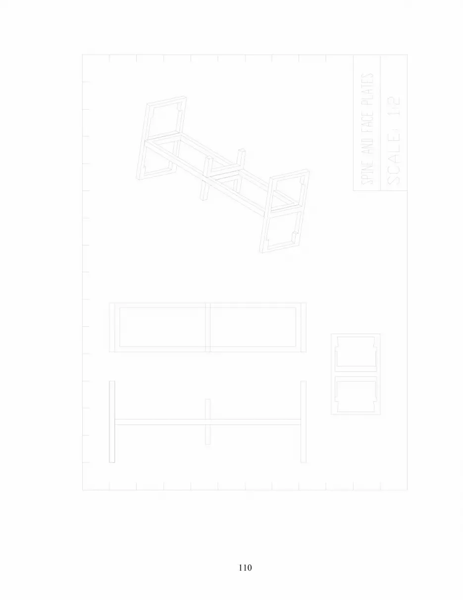
110

111

112

113

114

115

116

117

118

119

120

121
APPENDIX B – MATERIALS LISTS AND COSTS
Manufacturing Materials
Description Qty Price Total 18-8 SS button head socket cap screw 2.56 thread x 1/4" length (pkg. 100ea.) 1 $7.95 $7.9518-8 SS button head socket cap screw 4-40 thread x 3/8" length (pkg. 100ea.) 1 $4.54 $4.5418-8 SS button head socket cap screw 6-32 thread x 3/8" length (pkg. 100ea.) 1 $5.68 $5.6818-8 SS button head socket cap screw, 2-56 thread, 1/4" length (pkg. 100ea.) 1 $7.95 $7.9518-8 SS button head socket cap screw, 2-56 thread, 3/8" length (pkg. 100ea.) 1 $9.04 $9.0418-8 SS button head socket cap screw, 2-56 thread, 316" length (pkg. 100ea.) 1 $7.81 $7.8118-8 SS button head socket cap screw, 2-56 thread, 5/8" length (pkg. 100ea.) 1 $13.23 $13.2318-8 SS precision hex socket shoulder screw, 1/8" shoulder dia., 1/2" long shoulder, 4-40 thread 2 $1.62 $3.2418-8 SS precision hex socket shoulder screw, 1/8" shoulder dia., 1/8" long shoulder, 4-40 thread 4 $1.19 $4.7618-8 SS precision hex socket shoulder screw, 3/16" shoulder dia., 3/8" long shoulder, 8-32 thread 20 $1.57 $31.4018-8 SS precision hex socket shoulder screw, 3/16" shoulder dia., 1/8" long shoulder, 8-32 thread 10 $1.17 $11.7018-8 SS precision hex socket shoulder screw, 3/16" shoulder dia., 1/8" long shoulder, 8-32 thread 6 $1.17 $7.0218-8 SS small pattern machine screw nut 6-32 screw size, 1/4" width, 3/32" height (pkg. 100ea.) 1 $3.18 $3.1818-8 stainless steel large-OD flat washer 6 screw size, 9/64" ID, 5/8" OD, .031" thick (pkg. 100ea.) 1 $4.47 $4.4718-8 stainless steel machine screw nut 2-56 screw size, 3/16" width, 1/16" height (pkg. 100ea.) 1 $2.35 $2.3518-8 stainless steel shoulder screw, 5/16" shoulder dia., 1-1/4" long shoulder, 1/4"-20 thread, hardened 4 $2.06 $8.24Alloy 6061 aluminum rectangular bar, 1/2" thick x 3" width x 6' length 1 $44.68 $44.68Alloy 6061 aluminum rectangular bar, 1/8" thick x 4" width x 6' length 1 $24.04 $24.04Alloy 6061 aluminum rectangular bar, 3/16" thick x 4" width x 6' length 1 $28.94 $28.94Aluminum flat washer 2/56" screw size, grade 1100-F, .328" ID, 7/8" OD, .0635" thick (pkg. 100ea.) 1 $7.58 $7.58Aluminum threaded round standoff 1/4" OD, 1/8" length, 6-32 screw size 50 $0.23 $11.50Aluminum unthreaded round spacer 1/4" OD, 3/16" length, #8 screw size 10 $0.20 $2.00Aluminum unthreaded round spacer 5/16" OD, 3/16" length, #10 screw size 10 $0.54 $5.40

122
Manufacturing Materials (cont.) Description Qty Price Total FSHT1R single aluminum horn, red, 1" 4 $5.99 $23.96Low-carbon precision ground flat stock 3/32" thick, 1/2" width, 2ft. Long 1 $6.65 $6.65Metric cheese head slotted machine screw 18-8 SS, M3 size, 8mm length, .5mm pitch (pkg. 100ea.) 1 $5.32 $5.32Metric cheese head slotted machine screw 18-8 SS, M4 size, 10mm length, .7mm pitch (pkg. 100ea.) 1 $7.42 $7.42Rigid-carbon filled garrolite sheet 1/16" thick, 12" x 24" 1 $108.08 $108.08Sharp GP2D120 IR Sensor 2 $12.50 $25.00Spring lock washer 6 size, .148" ID, .25" OD, .031" min. thickness (pkg. 100ea.) 1 $4.79 $4.79Type 302 Stainless steel wire rope 1x7 strand, 1/32" dia, 150lb breaking strength 10 $0.05 $0.50Type 302 Stainless steel wire rope 7x7 strand core, 1/32" dia, 130lb breaking strength 10 $0.25 $2.50White PTFE flat washer, #12 screw size, .250" ID, .500" OD, .057" min. thickness (pkg. 10ea.) 1 $4.09 $4.09White Teflon flat washer, #8 screw size, .187" ID, .500" OD, .0355" min. thickness 1 $3.55 $3.55Zinc-plated copper oval compression sleeve for 1/32" wire rope, 1/4" sleeve length 1 $3.11 $3.11
Electronic Components Description Qty Price Total 2-LI 2200 Pack 7.4v Li-Ion w/22 AWG 4 $30.00 $120.006 Volt regulator MK II, universal for Hitec/JR/FJ 2 $19.50 $39.00BEC (JST) female plug 2 $2.50 $5.00BEC (JST) male plug 2 $2.00 $4.00BrainStem GP 1.0 Module 2 $79.00 $158.00CH830 DC/DC Li-Ion charger 1 $29.99 $29.99FSR, Design Kit, 400 series 1 $79.95 $79.95MX-450MG Hi-torque metal gear servo, Futaba J 6 $36.99 $221.94MX-450MG Hi-torque metal gear servo, Futaba J 26 $36.99 $961.74PAN serial cable replacement (pre-paired) 1 $199.00 $199.00RC Servo 1 $19.00 $19.00

123
Tools Description Qty Price Total 0-1/4" capacity T-type tap wrench w/guide 1 $10.95 $10.951/32" bevel tip for 7694A41 & A65 pencil-grip economy butane soldering torch 1 $9.00 $9.0012pc .050-5/16" w/holder allen short arm hex key set 1 $5.09 $5.092-56 plug H2 ground thread hand tap 2 $3.30 $6.603/32" bevel tip for 7694A41 & A65 pencil-grip economy butane soldering torch 1 $9.00 $9.004-40 plug H2 ground thread hand tap 2 $1.79 $3.584pc universal set Noga deburring tools 1 $9.20 $9.206-32 plug H2 ground thread hand tap 2 $1.75 $3.508-32 3 flute plug USA H2 had tap 2 $3.94 $7.88Escali 136DS postal/kitchen scale 13lb. 1 $38.95 $38.95Glider single lens safety glasses 135mm clear fog-free lens w/blue nylon frame 2 $6.70 $13.40Glider single lens safety glasses 135mm clear fog-free lens w/blue nylon frame 2 $6.70 $13.40Machine screw size high-speed steel hand tap taper, 2-56, H2 pitch diameter, 3 flute 2 $5.97 $11.94Machine screw size high-speed steel hand tap taper, 4-40, H2 pitch diameter, 3 flute 2 $3.77 $7.54Miniature electronics hex driver 8 piece set, includes sizes .028" thru 1/8" 1 $21.20 $21.20Miniature electronics metric hex driver 7-piece set, includes sizes 0.7mm thru 3.0mm 1 $19.18 $19.18no. 50 black nitrided HS job drill 12 $0.40 $4.75No-clean flux core solder 63% tin, 37% lead, .031" wire dia. 1lb. Spool 1 $12.78 $12.78Pencil-grip economy butane soldering torch kit w/4 tips, wiping sponge, safety stand & case 1 $54.05 $54.05Premium solid carbide end mill, sq. end, 2 flute, 1/8" mill dia., 1-12" length overall 4 $6.73 $26.92Pro-value satin-chrome steel machinists' rule rigid, inch/metric, 150mm/6" length, 3/4" width 1 $7.58 $7.58Pro-value satin-chrome steel machinists' rule semi-flex, inch/metric, 150mm/6" length, 1/2" width 1 $7.25 $7.25Single groove hand tool for oval/stop sleeves for 1/32" copper, zinc-plated copper 1 $39.98 $39.98Soldering iron tip tinner/cleaner, lead free, .7oz. Can 1 $3.62 $3.62Standard desoldering braid, 7/64" width, 5' length 1 $2.72 $2.72
Materials Total: $2,289.29 Tools Total: $336.66 Tax, Shipping & Handling: $197.00 Grand Total: $2,822.95