project appraisal manual
TRANSCRIPT
Project Appraisal Manual
January 2013 Baghdad, Iraq
Project Appraisal Manual
2
Table of Contents
PREFACE ........................................................................................................................... 4 Chapter I: Introduction ........................................................................................................ 6 Chapter II: Project Development and Approval Cycle ....................................................... 9 Chapter III: Project Evaluation Framework ...................................................................... 25 Chapter IV: Schematic Diagram ....................................................................................... 34
Chapter V: Project Evaluation Criteria ............................................................................. 44 Chapter VI: Financial Analysis of a Project ..................................................................... 61 Chapter VII: Financial Cost of Capital ............................................................................. 95 Chapter VIII: Risk Management ..................................................................................... 137 Summary of Project Appraisal Results ........................................................................... 150
Appendixes ..................................................................................................................... 154
Appendix 1: Economic Externalities .............................................................................. 155 Appendix 2: Estimation of Economic Prices or Tradable Goods and Services .............. 171
Appendix 3: Estimation of Economic Prices for Non-Tradable Goods and Services .... 182
Appendix 4: Estimation of Economic Prices For ........................................................... 208 Goods & Services in regulated markets .......................................................................... 208 Appendix 5: Evaluation of Stakeholder Impacts in Cost Benefit Analysis .................... 211
Appendix 6: Opportunity Cost of Foreign Exchange ..................................................... 218 Appendix 7: Economic Discount Rate ............................................................................ 227
Appendix 8: Economic Opportunity Cost of Labor ........................................................ 231
Project Appraisal Manual
3
FOREWORD
An Overview of the Manual
The manual has been divided into three parts.
Part I will focus on the theory and
methodology of project development and appraisal (cost-benefit analysis); examples will
be provided to illustrate many of the points. Users of this manual will hopefully go back
and forth between the theory and the case studies to gain a thorough understanding of
how to apply the principles of project evaluation to the analysis of investment
opportunities in the public sector.

Project Appraisal Manual
4
DRAFT, January, 2013
PREFACE
Why develop this manual?
The purpose of this manual is to help the Iraqi government implement the use of
international best practices of Project Appraisal while approving a public sector project.
It describes how public sector investments should be evaluated so that they may be taken
from the idea stage to the implementation phase in a successful manner. These themes
will be addressed under three headings: financial, economic, and distributional analysis
of a project.
By their very nature, investment projects involve benefits and costs over a number of
years into the future. Market prices and project outcomes cannot be predicted with
certainty. In addition, technical difficulties and delays in implementation frequently
result in cost and time overruns. Given this uncertainty, account must be taken of a
project’s risks and the costs that these risks create. Risk analysis, and how to reduce and
manage risk through the use of contracting, and other risk mitigation methods, will
constitute the fourth part of the manual.
What is the manual?
The manual is a supplement to training of those employees who are not familiar with the
methodology of project selection using Net Present Value (NPV) criteria. It helps
employees of the operating departments understand the methodology for viable project
selection. The Manual contains an introduction to project appraisal techniques, a detailed
discussion on financial, economic, stakeholder and risk analysis, and some practical
recommendations on how to proceed.
When to use the manual?
Once a line ministry has decided to adopt this methodology for approving capital
investment projects, this manual can and should be used as a reference book.
Who should use the manual?
This manual is intended for a number of users in all ministries which have capital
investment projects. First, it serves as a guide to the public sector managers responsible
for making public sector investment decisions. This group includes not only project
analysts and decision makers within the ministries of planning and finance, but also those
employed in the line ministries, and government departments and agencies that are
involved with the formulation, evaluation and implementation of projects. Second, the
Manual is meant to be used for training purposes by training institutions to educate and
train the future managers in these states. Finally, it provides an assurance to the
international development and lending institutions that the funds provided to the states
will be spent in a responsible and productive way.

Project Appraisal Manual
5
The manual will be intended for a number of users. First, it serves as a guide to public
sector managers responsible for making public sector investment decisions. This group
includes not only project analysts and decision makers within the ministries of planning
and finance, but also those employed in the line ministries, and government departments
and agencies that are involved with the formulation, appraisal and implementation of
projects. Second, the manual is meant to be used for training purposes by the training
institutions to educate and train the future managers in these states. Finally, it provides an
assurance to the international development and lending institutions that the funds
provided for capital investment projects will be spent in a responsible and productive
way.
How to use the manual?
The manual is most effective when combined with employing a competent consultant
who can conduct training and provide technical assistance to department employees
appraising the projects for the first time using this methodology. Accordingly, it is best
used in conjunction with a formal implementation plan and training program. Employing
specialists who have had experience with the approach would significantly augment
implementing this methodology. Finally, there is a step-by-step guide and a checklist
that can help assure that the process remains on track.

Project Appraisal Manual
6
Chapter I: Introduction
Project Appraisal Manual
7
CHAPTER I: INTRODUCTION
Purpose of the Project Appraisal
Manual
The purpose of the Project Appraisal
Manual is to help the Government of
Iraq develop and evaluate investment
projects to promote economic and social
well-being. It describes how public
sector investments should be evaluated
so that they may be taken from the idea
stage to the implementation phase in a
successful manner. These themes are
addressed under three headings:
financial, economic, and distributional
analysis of a project.
By their very nature, investment projects
involve benefits and costs over a number
of years into the future. Market prices
and project outcomes cannot be
predicted with certainty. In addition,
technical difficulties and delays in
implementation frequently result in cost
and time overruns. Given this
uncertainty, account must be taken of a
project’s risks and the costs that these
risks create. Risk analysis, and how to
reduce and manage risk through the use
of contracting, and other risk mitigation
methods, constitutes the fourth part of
this Manual.
The Targeted Users of the Manual
This manual is intended for a number of
users. First, it serves as a guide to public
sector managers responsible for making
public sector investment decisions. This
group includes not only project analysts
and decision makers within the
ministries of planning and finance, but
also those employed in line ministries,
and government departments and
agencies that are involved with the
formulation, evaluation and
implementation of projects. Second, this
Manual is meant to be used for training
purposes by the training institutions to
educate and train the future managers in
these states. Finally, it provides an
assurance to the international
development and lending institutions
that the funds provided will be spent in a
responsible and productive way.
What is a Project?
In capital budgeting, a project is the
smallest, separable investment unit that
can be planned, financed, and
implemented independently. This helps
to distinguish a project from a program
that may consist of several inter-related
or similar investments. While it is
possible to treat the whole program as a
project for the purposes of analysis, it is
advisable to keep projects limited in
scope and close to the minimum size that
is economically, technically and
administratively feasible. If a project
approaches program size, there is a
danger that a highly profitable
component may mask an unprofitable
activity.
In general terms, project refers to a great
variety of activities that may range from
single-purpose activities such as small
infrastructure projects to more complex
multi-part projects such as integrated
hydro-electric projects with irrigation,
power and tourism as its components.
For the purposes of this manual, a
Project Appraisal Manual
8
project may be defined as “an activity
that involves the use of scarce resources
during a specific time period for the
purpose of generating socio-economic
return in the form of goods and
services.” Thus a project may be viewed
as an investment that encompasses not
only the physical infrastructure facilities
such as roads, irrigation canals and
drinking water facilities but also
development services such as agriculture
extension, health and education.
Project as an “Incremental” Activity
An investment opportunity usually
involves incremental net cash outflows
or economic costs in the initial
investment or construction phase
followed by incremental net cash
inflows, or net economic benefits, in the
operating phase. An incremental net cash
flow refers to the net cash flow, or net
economic benefit that occurs with a
project minus
the net cash flow, or net
benefit that would have occurred in the
absence of the project. In this way, it is
possible to identify the additional net
cash flow, or net economic benefit that is
expected to arise as a result of an
additional or new investment through a
project and to measure the
corresponding change in wealth, or in
economic well being that can be
attributed to it.
Uncertainty and Contractual
Arrangements
Although this is the standard view of a
project, and one that will be analyzed in
the chapters related to the financial,
economic and distributive analyses it is
not the complete picture. Uncertainty
prevents an analyst from precisely
identifying the time path of the net cash
flows or net benefits. The best that can
be said is that the anticipated benefits
and costs are likely to lie in a given
range with a given probability. Thus,
the
output of a project appraisal is more than
just a point-estimate of a project’s net
return. A project evaluation should
provide some assessment of the expected
variability of a project’s net return, the
probability of a negative return, the cost
of risk and who is likely to bear it.
Even with this information, the profile of
a project is not complete. There is also a
need to know and understand a project’s
contractual environment. For example,
there may be alternative financing
arrangements that would help to
redistribute some of the risk and make a
project more attractive. Or there may be
contracts that project managers enter
into with its customers/end-users or its
suppliers. These different arrangements
could also create incentives or
disincentives that would encourage a
project’s participants to alter their
behaviour and change the overall
returns.
The effects of this uncertainty and the
contractual arrangements are an integral
part of project appraisal and are dealt
with in the risk analysis part of the
manual.
Project Appraisal Manual
9
Chapter II: Project Development and Approval
Cycle
Project Appraisal Manual
10
CHAPTER II: PROJECT DEVELOPMENT AND APPROVAL
CYCLE
Project Development Cycle
Every project has certain phases in its
development and implementation. These
phases are useful in planning a project as
they provide a framework for resource
allocation, scheduling project milestones
for implementation, and establishing a
monitoring system. The purpose is to
provide a basis for organizing the project
for establishing resource requirements,
and set up the management system that
will finally guide the project activities.
The phases of project development are
commonly referred to as the project
development cycle or project life cycle.
The project life cycle phases may be
broadly placed in the following
categories:
(a) Concept or identification
(b) Definition or preparation
(c) Pre-feasibility
(d) Feasibility and financing
(e) Detailed design
(f) Implementation and monitoring
(g) Ex-post appraisal and impact
evaluation
In the concept or identification phase,
the public sector manager evaluates an
idea. In the definition or preparation
phase, it elaborates and refines the
concept and does some initial work to
define the components that make up the
project. The pre-feasibility and
feasibility phases comprise a more
analytical exercise in which the viability
of the project is examined from different
points of view and the project is planned
in detail. These two phases of the
project cycle taken together mainly
constitute the process of evaluation or
appraisal of the project.
In the next phase of detailed design, the
physical design of the project is
completed and the plan for
administration, operations, and
marketing is finalized. The bulk of the
actual work on the project is, of course,
accomplished in the implementation
phase. Finally, a critical evaluation of
the project’s outputs and outcomes is
conducted in the last phase. As the
project moves through its life cycle, the
focus of managerial activities shifts from
planning to operating and controlling the
activities.
It should be emphasized that these
phases only represent a natural order in
which projects are planned and carried
out and they are not sequential. Also,
several of these phases do not become
final until the project approaches its
termination stage. The project
development cycle is a continuous and
dynamic process and there is a great deal
of overlap, interaction and feedback
among the various phases. Many of the
activities are inter-related and cannot be
confined to one particular phase.
Projects and State Development Plans
Projects provide a valuable tool for
directing investments into the priority
sectors of an economy. A state or
regional plan lays down growth targets
for various economic parameters like
consumption, public and private sector
investments and gross state product. This
Project Appraisal Manual
11
exercise of macroeconomic planning is
meaningful only when it is possible to
make realistic assumptions about the
level of investment that can be achieved
in a certain period of time and its impact
on the rate of growth. This presupposes
knowledge of the existing and potential
projects in the state sector and the pace
at which they may be implemented.
It is also the main objective of the
planning process to direct investment to
those sectors where it will yield the
maximum economic benefits to the state.
Again, within a sector priority needs to
be given to projects with the highest
economic returns. It is possible to make
this kind of judgment only with the help
of economic analysis of projects. Thus
the planning process is hardly relevant
without project planning and without a
rigorous analysis at the sector and
project levels1.
The reverse linkage between projects
and plans is equally strong. For making a
choice among projects, it would be
necessary to estimate the market demand
for the goods and services produced by
those projects. Thus the microeconomic
planning at the project and sectoral
levels clearly depends upon how the
overall economy is likely to develop in
the course of time which, in turn, is a
function of the long range plans and
policies of the state government2. Thus
1 See Little, I. M. D. and J. A. Mirrlees; “Project
Appraisal and planning for Developing
Countries”, Basic Books, Inc., New York (1974)
for a discussion on the strong inter-linkage
between plans and project choice. 2 See Kaufmann, D. and Yan Wang,
“Macroeconomic Policies and Project
Performance in the Social Sectors: A Model of
the analysis of a project within the
overall framework of a state plan should
be more realistic as compared to a
situation where no plan exists.
This clearly indicates a close interaction
between project analysis and plan
formulation3. A plan may be initially
formulated without an adequate
knowledge of the role of individual
projects or sectors in the overall growth
of the economy. This will sharpen the
focus of the micro level planning. An
improvement in the analysis of projects
and sectors will help improve the quality
of macroeconomic management. Thus
there is a feedback process between
project analysis at the micro level and
planning at the macro level.
Concept or Identification Phase
This is the first phase of the project cycle
and is concerned with the identification
of potential projects. The purpose is to
establish the basic desirability of a
project and identify the high priority
projects4. The type of projects that
would qualify for being placed in this
Human Capital Production and Evidence from
LDCs,” World Bank (1995). 3 The integration between project planning and
national or macro-level planning has been a
significant issue in the literature on project
analysis. At the micro level the individual
projects have to be feasible while at the macro
level a set of projects has to be selected that are
collectively feasible and fit into a national
perspective. See Noorbaksh (1993) for an
excellent discussion of this issue. 4 Baum, Warren C., “The World bank Project
Cycle”, in Finance and Development delineates
and discusses the phases of the project cycle in
the context of World Bank funding of public
sector projects.
Project Appraisal Manual
12
category will largely depend upon the
level of development of the economy.
States and regions differ with respect to
their problems as well as their growth
potential.
Action Points in Project Identification
The identification process implies
undertaking of two sets of activities.
First, the gaps in the economy should be
identified and second, the sector
priorities should be defined. These
activities are truly dynamic in nature and
keep evolving over time. Both these
tasks are routinely performed during the
planning process at the state, regional or
district level. A thorough analysis of the
gaps in development and the potential
for growth is undertaken at the time of
plan formulation and during periodical
reviews. This also enables a continuous
assessment of the progress and the
shortfalls and provides valuable
feedback to the policy makers.
The gaps in the economy could lie in one
or more sectors such as basic
infrastructure, food and agriculture,
heavy or basic industry, or social sectors
such as health and education. In practice,
the identification of gaps is not a
difficult task. What is difficult is the
setting up of a clear priority among
competing claims on the limited
resources of the state or the region. This,
in fact, constitutes the crux of the
development problem and is the most
difficult challenge that planners and
policy makers face.
Problems in Project Identification
The following set of problems is often
encountered in the process of project
identification.
Resource surveys and project
identification5: The lack of finances and
scarcity of skilled manpower has acted
as a major deterrent in carrying out
detailed resource inventories that are
needed for identifying projects and for
rationalizing development plans. This is
more so in agriculture, rural industries
and natural resources sectors where
detailed information can be obtained
only after sustained research and survey
work. There has been a tendency to
move ahead with investments in certain
sectors perceived as lead sectors, such as
industries, rather than spending
resources on research and surveys that
would identify higher return areas that
are perhaps not as obvious. For
example, the rate of return on road repair
and rehabilitation projects have tended
to be much greater than the rate of return
for new roads but the rehabilitation
projects usually do not get due priority.
The emphasis is mostly on initiating new
projects.
Lack of skills to produce project
alternatives: While capital scarcity is
one of the main constraints, the problem
of project scarcity is equally serious.
Often, human resources do not exist in
the state or the region for identifying
suitable project interventions that are
required to fulfill the plan objectives and
5 Ward, William A., and Barry J. Derren, “The
Economics of Project Analysis: A Practitioner’s
Guide”, Economic Development Institute of the
World Bank (1991) presents an excellent
analysis of the various aspects of strategic
planning and project appraisal.
Project Appraisal Manual
13
achieve the development goals. Thus,
there may be simply a lack of skills to
produce project alternatives.
Sources of Project Identification
A project may be identified in a variety
of ways.
(i) Conceived by existing
departments or ministries in the
government,
(ii) Emerge out of the process of
formulation of plans at the
national and provincial levels,
(iii) Identified by the people’s
representatives, and,
(iv) Proposed as a demand from
interest groups or beneficiaries.
Preparation Phase
Once a project is identified, the process
of preparation is initiated. This process
involves the refinement of the elements
described in the identification phase and
includes all the steps that are necessary
to bring the project to the stage of
appraisal, which would consist of pre-
feasibility and feasibility studies. While
it is difficult to generalize about the
preparation phase as it depends upon the
nature of the project, preparation begins
with the description of objectives,
identification of the principal issues and
setting up of a timetable for the different
phases of development cycle. While
many of these issues would have already
been considered at the identification
phase, all these aspects are addressed in
greater detail during the preparation
phase and concrete answers are sought to
the various questions that arise in the
context of the project.
It may be noted that the process of
preparation must cover the full range of
technical, institutional, financial and
economic issues that are relevant to
achieving the project’s objectives. For
instance, an irrigation project would
require a study of several aspects such as
the existing soil patterns and available
water resources, appropriate cropping
patterns for the area based on data
available with the agriculture
department, impact of the facility on a
typical farm budget, extension services
in public and private sectors, marketing
infrastructure in the region, existing land
tenure systems etc.
Policies and Procedures
Sometimes it may be necessary to
examine the government policies and
procedures that would have a major
impact on the outcomes of the project.
Also, sociological studies may be needed
to ensure that the project fits into its
physical and social environment so that
its benefits are maximized. In the case of
the irrigation project, for example, the
government policies with respect to
prices of inputs and agricultural
products, the method for determination
of user charges from the beneficiaries
and the procedure for collecting these
charges would have to be examined.
Technical and Institutional Alternatives
An important element of preparation is a
critical assessment of the technical and
institutional alternatives for the project.
This is essential for the choice of an
appropriate technical package necessary
to implement the project and
Project Appraisal Manual
14
identification of the agency or unit that
would be responsible for project
management. The choice of technology
will largely depend upon the resource
endowments of the national and local
government and the stage of its
development. For instance, most local
governments suffer from a lack of
capital but are abundant in labor. Thus
some types of advanced technology may
not be the most suitable for the specific
state or region. The preparation phase
requires an analysis of the benefits and
costs of the technical and institutional
alternatives followed by a more detailed
investigation of the more promising
alternatives. The process continues till
the most satisfactory solution is arrived
at.
It is evident that this process of project
preparation is both time consuming and
requires trained staff and financial
resources. Each project means a long-
term commitment of scarce resources
and serious economic implications for
the state. Therefore, the time and money
spent in selecting the most suitable
technical and organizational alternative
is well spent because over the long term
this effort will most likely be returned
many times over by the enhanced return
from the investment.
Pre-feasibility Phase
The preparation stage should be
followed by the pre-feasibility phase.
The pre-feasibility study is one of the
two components of appraisal, the
feasibility study being the other one.
This is the first attempt to examine the
overall potential or viability of the
project. The data and information
gathered at the preparation stage are
used in this phase. It is a critical stage of
the project cycle because it is the
culmination of all the preparatory work
and provides a comprehensive review of
all aspects of the project before taking a
final decision about its viability.
The pre-feasibility study is the stage for
completing all the preliminary steps for
going into a detailed feasibility exercise.
Thus, it is the first part of conducting the
appraisal of a project. Also, if a project
does not prove to be promising at this
stage, it may be rejected without
investing any additional time and
resources into its further examination
and the process of appraisal is over for
the project.
The pre-feasibility phase should
normally comprise of the following
modules6:
Marketing or Demand module
This module examines whether there is a
demand for the goods/services of a
project both in the domestic market, and
the neighboring states. In many states, it
is not unusual to come across defunct
projects that were taken up because of
political expediency or availability of
funds from the central government for
that type of projects but there was not
sufficient demand for the good or service
produced at that time to enable the
project to become either financially or
economically sustainable.
6 See Jenkins, et al. (1998) for a discussion of
the various aspects of project planning or the
pre-feasibility phase.
Project Appraisal Manual
15
The function of this module is not only
to assess the current demand but also to
undertake the more difficult task of
forecasting the future demand. For the
demand analysis of a product or service,
it is necessary to conduct some primary
research at the pre-feasibility stage by
surveying the potential customers and
users.
In the case of public sector monopolies,
such as public utilities, government
policies are an important factor in
determining the demand for the output.
Programs like electrification of rural
areas and promotion of industrial
complexes in urban areas will have an
important bearing on the future demand
for electricity. The growth in demand
for the output of a public utility may be
forecast fairly accurately by studying the
relationship over time of demand with
respect to variables such as population
growth, disposable income, industrial
output, and relative prices. The study of
growth in demand experienced by
utilities in other states can also provide a
good indication of what to expect in the
future.
Technical or Engineering Module
It looks at the input parameters of the
project, quantities and prices of inputs
by type required for construction of the
project, inputs required for the operation
of the project by year and volume of
sales or service delivery, and the
appropriateness of the technology
adopted. It is also concerned with issues
such as the size of the project, its design
and location and the technology to be
adopted including the equipment used
and the processes employed. In a canal
system for irrigation, for instance, this
module will be concerned with the size
and gradient of the main canals, the
volume of expected water flow at the
source, locations and numbers of
secondaries, impact on the water table in
the region and the availability of
drainage facilities for excess water.
A major task in this phase is to conduct a
close scrutiny of the cost estimates of
construction along with the engineering
data used to arrive at those estimates,
provisions for contingencies and
expected price increases during the
implementation phase and cost estimates
for operating the facilities. The
procedures for procurement of materials
and provision of professional services
are also reviewed at this stage.
The output from the technical module of
a pre-feasibility study should provide the
following information:
Environmental Module
Several projects have a negative impact
on the environment that may affect a
group of people in the society adversely.
This is an externality generated by the
project and is not reflected in the private
costs of the project. Industrial firms and
infrastructure projects, such as power
and transport, create different kinds of
pollution that fall in this category. Some
projects may deposit a lot of waste
products or effluents in the atmosphere,
waterways and the ground and these may
have serious health implications. Again,
the emissions from some projects have
long-term impact on the global climate
that may prove to be irreversible. All
these have a damaging effect on people
Project Appraisal Manual
16
and property that are not directly
involved with the production or
consumption of the output. The waste
products emitted by one producer may
adversely affect the production processes
of other firms or well being of other
consumers.
While this externality may not concern
the private producer unless its cost is
internalized through some mechanism of
regulation, tax or subsidy, it certainly
imposes a cost on the society and must
be taken into account when the project is
examined from the point of view of the
economy. If this aspect of costs were
ignored, investments that are not socially
desirable would appear to be attractive
and are likely to be included in the
state’s portfolio of development projects.
Whenever the project has an impact on
the environment, all costs of pollution
control equipment and facilities should
be included in project cost. Whatever
residual pollution and environmental
impacts remain after the pollution
control equipments are in place should
be estimated and its economic value
assessed. Finally, these values should be
included as a cost in the economic cash
flow of the project.
Manpower and Administrative Support
Module
This module goes into the manpower
requirements both for construction and
operation phases of the project. It
reconciles the technical and
administrative requirements of the
project with the supply constraint on
manpower.
It is a mistake to confine project
appraisal to the analysis of financial and
economic costs and benefits under the
assumption that the project can be built
and ready for operations on time. This
assumes a degree of administrative
support for implementation of projects
that in many states and regions does not
exist. Many projects have failed because
they were undertaken without the
administrative expertise necessary to
complete the project as specified. The
prospect that future financial and
economic benefits will materialize is
only as good as the administrative
capability of the agency in charge to put
the project in place.
This module must reconcile the technical
and administrative requirements of the
project with the supply constraints on
manpower. A careful study of the labor
markets should be made in order to
ensure that the estimates of wage rates to
be paid are accurate and that the planned
source of manpower is reasonable in the
light of labor market conditions. In
general, manpower requirements should
be broken down by occupational and
skill categories and these needs should
be evaluated in terms of the possible
sources from which they would be met.
Institutional Module
This module deals with the creation of a
local institution responsible for
managing the different stages or phases
of the project. This local institution does
not cover the borrowing entity and its
organization alone, but it includes the
entire management that goes into the
project along with its policies and
procedures. In a broad sense, the
Project Appraisal Manual
17
institutional set up also incorporates the
whole range of government policies and
procedures. Experience shows that
insufficient attention to the institutional
aspects creates serious problems during
the implementation and operations
phases of the project.
Financial Module
This module provides the first
integration of financial and technical
variables estimated in the marketing,
technical and manpower modules. A
cash flow profile of the project is
constructed, which identifies all the
receipts and expenditures that are
expected to occur during the lifetime of
the project. An attempt should be made
at this stage to provide a description of
the financial flows of the project that
identifies the key variables to be used as
input data in the economic and social
appraisal.
The financial appraisal also helps in
determining the level and structure of
prices or user fees to be charged from
the beneficiaries in order to ensure the
project’s financial viability. If the
facility is publicly owned and provides
some basic service, this question
becomes more important. Sometimes
governments decide to subsidize specific
services to consumers as a matter of
policy or pure expediency. The recovery
of user charges has to take into account
the income level of the beneficiaries and
the practical problems of administering a
particular system. The degree of fiscal
impact of such government policies on
the budget has a strong bearing on the
viability and sustainability of the project.
In such cases, not only should the level
and structure of prices be defined but
also the procedure for making future
adjustments in prices and government
subsidy should be clearly laid down.
For instance, in an irrigation project the
policy and procedure for recovering the
investment and operating costs from
farmers or water users is a matter of
concern to the financing agencies
including foreign donors and
international agencies. Costs in this case
may be recovered in a variety of ways:
user charges from beneficiaries based on
volume of use or area under irrigation,
general taxation or requiring the farmers
to sell all or part of their produce to a
government marketing agency at a price
controlled by the government. Each
particular policy will have different
implications for the level and efficiency
of cost recovery and the ultimate
financial viability of the project.
The financial module should answer a
series of questions concerning the
financial prospects and viability of the
project.
i. W
hat degrees of certainty do we
place on each of the revenue and
cost items in the financial
analysis? What factors are
expected to affect these
variables?
ii. I
n case of public utilities or
services provided by a public
enterprise, what should be the
level of user charges to ensure
the project’s financial viability
and what would be the necessary
Project Appraisal Manual
18
process and frequency of its
revision?
iii. W
hat sources of financing will be
used to cover the cost of the
project? Does this financing
have special features, such as
subsidized interest rates, grants,
foreign equity or loans (tied or
general)?
iv. I
s there provision for adequate
working capital in the project?
Will internal revenues be enough
for this purpose or will separate
institutional funds be required?
v. W
hat is the minimum net cash flow
required by this investment to be
able to continue operations
without unplanned requests being
made to the government treasury
for supplementary financing?
vi. D
oes the project have a large
enough net cash flow or financial
rate of return for it to be
financially viable? If not, what
sources of additional funds are
available and can be committed
to the project if it is economically
and socially justified but
financially poor?
If any one of these questions points to
future difficulties, then necessary
adjustments should be made in either the
design or the financing of the project to
avoid problems in future that may
adversely affect the project.
Economic Module
It examines the project from the entire
economy's point of view to determine
whether or not its implementation will
improve the economic welfare of the
country, the state or the region. An
economic appraisal is of exactly the
same nature as the financial analysis
except that now the benefits and costs
are measured from the point of view of
the whole economic entity, which could
be the country, the state or a specific
region. Instead of relying on market
prices to measure expenditures and
costs as in the case of a financial
appraisal, the economic analysis
requires the use of techniques to
determine the economic prices of goods
and service, foreign exchange, cost of
capital and labor. The true economic
values of costs and benefits are not
reflected in market prices in the
presence of various distortions such as
trade restrictions, price control, taxes,
subsidies, and minimum wages.
Some of the elements of project costs
and benefits such as environmental
pollution, better health and education
facilities, manpower training may not be
easy to quantify. The best approach in
such cases would be to find people’s
willingness to pay for the service or their
willingness to pay for avoiding a
negative outcome. The willingness to
pay also provides a valuable benchmark
for determining the financial level of
user charges for services. The financial
charges may be raised to the level of the
economic prices because the latter
indicate the benefit that people derive
from the good or service in question and
Project Appraisal Manual
19
their willingness to pay for the same. It
is, however, not always easy to get a
measure of the willingness to pay. In
some cases, it may be possible to have
proxies that help measure people’s
willingness to pay and thereby estimate
the value of a service to the economy.
The questions covering the economic
appraisal of a project are as follows.
i. W
hat are the magnitudes of the
differences between the financial
and economic values of variables
that are affected by government
regulation and control or are
subject to taxes, tariffs, and
subsidies?
ii. W
hat are the magnitudes of the
differences between the financial
and economic values of variables
that are affected by other
imperfections in the factor and
product markets (e.g., labor
unions and restrictive trade
practices)?
iii. W
hen evaluated at a discount rate
that reflects the relevant cost of
capital to the economy as a
whole, does this project produce
a positive net present value?
Social Appraisal or Distributive and Basic
Needs Analysis
This deals with the identification and
quantification, whenever possible, of the
impacts on the various stakeholders of
the project. These include impact on the
well being of particular groups in
society. While this aspect of the
appraisal may be less precise than the
financial or economic analyses of a
project, the social evaluation will
generally be tied to the same factors that
make up the financial and economic
appraisals. For example, a project
cannot be expected to assist consumers
unless it increases the supply of a good
or service at a price not greater than its
previous price.
The social appraisal of a project may be
organized into two parts; first, estimating
how income changes caused by the
project are distributed among the various
stakeholders to the project (distributional
analysis) and second, identifying the
impact of the project on the basic needs
in society (basic needs analysis). In
conducting a distributive analysis, the
net impact of all externalities, which is
the difference between the real economic
values of resource flows and their real
financial values, are measured for each
market in present value terms and
allocated across various stakeholders of
the project. Finally, additional net
benefits are attributed to the project if it
provides for one or more of the basic
needs. For instance, a road project in a
rural area not only reduces transportation
costs but it may also allow the children
to attend school and the sick to get better
health care. Both these aspects are
viewed positively by society and a social
net benefit should be attributed to the
project to account for this externality.
Nature of Distributive Analysis
In essence, a distributional analysis
combines the financial analysis for each
Project Appraisal Manual
20
group with its corresponding
externalities. The sum of the financial
outcome and the externalities generated
across the various groups should add up
to the economic analysis of the overall
project. In this way, it is possible to
identify those groups that gain and those
that lose and the extent of gain and loss
as a result of a project. It provides a very
valuable input to the policy makers.
Nature of Basic Needs Analysis
The basic needs externality can be
thought of as the price that society is
willing to pay for any increases in the
recipients’ consumption of particular
goods or services that contribute to the
fulfillment of basic needs. The
willingness to pay for basic needs can be
added vertically to the private demand
curve of the target group to create a
social demand curve.
An illustrative set of questions to be
asked while undertaking a social
appraisal of a project is as follows.
i. What social objective could the
project assist in attaining?
ii. Who are the beneficiaries of
the project and who is expected
to bear the costs?
iii. I
n what alternative ways and at
what costs could the government
obtain social results similar to
those expected from this project?
iv. W
hat are the (net) economic costs
of undertaking these alternative
projects or programs and is the
project relatively cost effective in
generation of desirable social
impacts?
v. W
hat are the basic needs of the
society that are relevant in the
country and what impact will the
project have on basic needs.
Use of Secondary Data in the Pre-
feasibility Phase
Whenever possible, the pre-feasibility
study should utilize secondary research
data. Most technical and marketing
problems have been faced and solved
before by others; therefore, a great deal
of information can be obtained quickly
and cheaply if the existing sources are
utilized efficiently. Secondary research
is probably most useful in the technical
and engineering modules but less
valuable in the marketing and the
manpower and administrative support
modules. Marketing and administrative
support modules generally require
information that is specific to the project
and may require some primary data.
Engineering firms and technical experts
in the field usually have considerable
experience in other projects that have
used either identical or similar
technology. Often there are a number of
consulting firms or government agencies
that have technical expertise in a specific
area. Utilization of the published
research materials on commodities and
technical aspects of projects from
international organizations and
institutions or associations disseminating
pertinent information is essential.
Project Appraisal Manual
21
Feasibility Study and Financing
Negotiations
After completing all the modules of the
pre-feasibility phase, the project must be
examined to see if it shows promise of
meeting the financial, economic, and
social criteria that the government has
set for investment expenditures. It is at
the end of this stage that the most
important decision has to be made as to
whether the project should be approved.
It is much more difficult to stop a bad
project after the detailed and, often,
expensive design work has been carried
out at the next stage of project
development. Once sizable resources
have been committed to prepare the
detailed technical and financial design of
a project, it takes very courageous public
servants and politicians to admit that it
was a bad idea.
If the outcome of the feasibility study is
such that the decision-makers give their
approval to the project, then the next
major steps are tying up the financing
and developing the detailed project
design. Negotiations about the financing
of the project have to be finalized with
all the financial institutions and a
detailed loan document drawn. The
drafting and negotiation of the legal
documents are essential for ensuring that
the borrower and the lenders are in
agreement not only on the terms of
financing but also on the broad
objectives of the project and the detailed
schedule and specific activities
necessary for implementing it.
Detailed Design
Preliminary design criteria must be
established when the project is identified
and appraised but usually expenditures
on detailed technical specifications are
not warranted at that time. Once it has
been determined that the project will
continue, the design task should be
completed in more detail. It involves
detailing the basic programs, allocating
tasks, determining resources and setting
down in operational form the functions
to be carried out along with their
priorities. Technical requirements, such
as manpower needs by skill class should
be finalized at this stage. Upon
completion of the blueprints and
specifications for construction of
facilities and equipment, operating plans
and schedules along with contingency
plans must be prepared and brought
together before going into the
implementation phase.
When this process is completed, the
project is again reviewed to see whether
it still meets the criteria for approval and
implementation. If it does not, then this
result must be passed on to the
appropriate authorities for final
disapproval or rejection of the project.
Project Implementation
If the appraisal and design have been
properly executed and negotiations to
finalize the conditions for financing
successfully completed, the formal
approval of the project is sought from
the competent authority. The formal
approval will require the acceptance of
funding proposals and agreement on
contract documents, including tenders
and other contracts requiring the
commitment of resources.
Project Appraisal Manual
22
The next stage in the project’s life cycle
is its actual implementation. This is,
evidently, the most important part of the
project cycle. The project
implementation phase covers both the
completion of construction activities and
the subsequent operations and is
generally divided into three different
time periods. First is the investment
period when the major project
investments take place. Second is the
development period when the production
capacity gradually builds up. The final
phase is that of full operations.
Implementation is a dynamic process in
which every one involved with the
project has to constantly respond to new
problems or changing circumstances that
may affect the project’s outcome.
The process of implementation involves
the coordination and allocation of
resources to make the project
operational. The project manager has to
bring together a project team including
professionals and technicians. This team
will, in turn, have to coordinate with the
various consultants, contractors,
suppliers and other interested agencies
involved in putting the project in place.
Responsibility and authority for
executing the project must be clearly
assigned. This will include the granting
of authority to make decisions in areas
related to personnel, legal and financial
matters, organization and administration.
Proper planning at this stage is essential
to ensure that undue delays do not occur
and that proper administrative
procedures are designed for the smooth
coordination of the activities required for
the implementation of the project.
A system of monitoring and supervision
has to be evolved for completing this
phase successfully and on time. This
task is very important because all
projects face some implementation
problems. The problems may arise either
because of some flaw or shortcoming in
the planning of the project or simply
because of changes in the economic and
political environment. The monitoring
takes place at various levels. The first
and the foremost level is the monitoring
by the project manager and his team.
This is done almost on a daily basis.
Again, there is periodic monitoring by
the higher management levels in the
department or the implementing agency
and also by the concerned ministries in
the government. Different sets of
criteria have to be evolved for
monitoring by the different levels of
supervisors within the organization and
outside.
Ex-post Appraisal and Evaluation
Historically, considerably more
resources have been spent on the pre-
evaluation of projects than on the review
of the projects actually implemented.
For the development of the operational
techniques of project appraisal and the
improvements in the accuracy of
evaluations, it is very useful to compare
the predicted performance with the
actual performance of projects. In order
that this review of the strengths and
weaknesses of implemented projects be
of maximum value to both policy makers
and project analysts, it is important that
some degree of continuity of personnel
be maintained within the project
evaluation teams through time.
Project Appraisal Manual
23
In carrying out ex-post appraisal, both
elements of success and failure are
systematically analyzed. It need not be
conducted only for completed projects,
but may take place at various stages
during the project’s implementation and
operational phase. A careful appraisal of
a project is a must before planning any
follow up projects. A final detailed ex-
post appraisal should, of course, be
undertaken after the project is
terminated.
To facilitate this type of appraisal, a
review of the administrative aspects of
the project development should be made
immediately after the project becomes
operational. The managers of the
operational phase of the project should
be made aware of the fact that an in
depth appraisal of the project’s
performance is to be carried out. This
ensures the development of necessary
data from an early stage and makes the
appraisal process quite cost effective.
The scope of ex-post appraisal is much
wider than an audit. The audit has an
important function and it should be
conducted immediately after the
construction phase is over and a
completion report is submitted. The
project’s outcome (net present value or
internal rate of return) should be re-
estimated on the basis of the actual
investment costs and the updated costs
of maintenance and operations. This,
however, is not sufficient to enable the
project management, the government
department or the parent agency to draw
meaningful lessons for design and
preparation of future projects.
The function of the post appraisal is not
only to assess the performance of a
project and give an ultimate verdict as to
its overall contribution to the state’s
development, but also to identify the
critical variables in the design and
implementation of a project that
determined its success or failure. It is
expected that well considered
recommendations would emerge from
the appraisal about improving each
aspect of the project design and its actual
implementation. Based on such
appraisal, ongoing projects may be
modified and subsequent projects in the
sector can be improved from the
experience of completed projects. Also,
new policies, better management
practices and improved procedures can
be adopted to improve project
performance in general.
Ex-post appraisal may be done by
different people who are directly or
indirectly involved with the project. The
project management, the sponsoring
government department or agency, the
operating ministry, the planning
organization in the government or an
external aid agency may be interested in
the process. Each of these agents has its
own lessons to draw from different
aspects of the project.
Finally, the evaluation of a project
involves an assessment of the outcomes
of a project or its impact on the
beneficiaries rather than simply the
measurement of the outputs of the
project. For instance, while the appraisal
of an irrigation project would involve an
analysis of costs and benefits to the
various stakeholders who are involved in
constructing the irrigation system, the
Project Appraisal Manual
24
evaluation would imply the study of
change in agriculture productivity in the
region. Similarly, the evaluation of a
school may involve an estimation of its
impact on literacy in the region rather
than simply looking at the number of
school going children. Thus the project
evaluation would often include pre- and
post- project benchmark surveys to see
how the project has been able to achieve
its overall objectives.
Project Appraisal Manual
25
Chapter III: Project Evaluation Framework
Project Appraisal Manual
26
CHAPTER III: PROJECT EVALUATION FRAMEWORK
Integrated Project Analysis
Traditional approaches to the appraisal
of investment projects have tended to
undertake the economic analysis in
isolation from the financial analysis, thus
ignoring the interaction of the financial
and economic outcomes. It is quite
common to find that the impact of
possible changes in the economic policy
environment has not been factored into
the design of the project and the
assessment of its risk. Consequently,
analysts have generally failed to identify
and make provisions for policy and
institutional variables that are important
determinants of the sustainability of
many of these investments. The
economic distortions that financially
subsidize a project, when removed, often
become a major source of failure for
these investments. Reduction in the level
of trade protection is a well-known
example of this problem.
The Integrated Project Analysis adopted
in this manual expands the scope of the
analyses of both public and private
sector projects beyond the traditional
practice of decision making on the basis
of the financial and economic net present
values of an investment. It demonstrates
that if the economic and financial
analyses are carried out using a common
numeraire, preferably expressing all
values in terms of the domestic prices at
the domestic price level, the scope of the
analysis can be expanded to include
issues of stakeholder impacts, poverty
impacts, and an assessment of the long-
term sustainability of the project.
Instead of just providing summary
statistics of the financial and economic
net present values for the project, we are
now able to assess the income impacts
that the project will have on different
interest groups in society.
An important contribution of this
analysis is that it forces the analyst to do
a reconciliation of the economic
performance, the financial performance
and the distributional impacts of a
project. If the economic and financial
analyses of a project have been done
consistently, the distributional
stakeholder analysis is a relatively
straightforward outcome. The benefit of
such an extension of the analysis is very
important for assessing the political-
economic dimensions of public sector
investments. The need for identifying
the project’s stakeholders, the groups
who will benefit from the project and
those who will lose, is crucial. A
project’s likelihood of successful
implementation or long term
sustainability is likely to be threatened if
specific groups in society are
unwittingly hurt by it. In many cases,
the most important factor determining a
project’s sustainability is its impact on
the government budget. For
sustainability, the project’s fiscal impact
must be consistent with the ability of the
public sector to finance such activities.
To undertake an integrated financial,
economic and distributive investment
appraisal or to evaluate the sustainability
of a project, two steps need to be taken:
Project Appraisal Manual
27
(a) First, the project’s financial profile
should be compared on a period-by-
period basis and not just summarized
in single statistics such as the NPV
or the internal rate of return (IRR).
Such summary criteria examined in
isolation do not accurately assess the
sustainability of a project or its
riskiness. Consider a project that has
both a large financial internal rate of
return (FIRR) and a large positive
NPV, but also has negative financial
cash flows in the early years of its
life. Such a project may go
bankrupt, jeopardizing its economic
performance, long before it has a
chance to generate the large positive
net cash flows expected in later
years. It is the examination of the
cash flows year by year over the
project’s lifetime that will give the
analyst an indication of the
sustainability and financial riskiness
of the project. If a project is not
financially feasible on its own, then a
realistic assessment of the degree of
budgetary support that it is likely to
receive from the government needs
to be made.
(b) Second, the financial and economic
analyses must be expressed in the
same unit of account. If we do not
use the same numeraire we cannot
successfully investigate the
differences between financial and
economic values of inputs and
outputs. If the units of account are
different for financial analysis and
economic analysis, then the
differences between the economic
and financial values have no
significance or meaning. In the
literature on benefit-cost analysis,
the three common choices for the
numeraire are: domestic currency at
domestic price level, domestic
currency at the border price level,
and foreign currency at the border
price level.
Financial analysis is usually performed
in domestic prices at the domestic price
level because these are the currency and
the price levels in which the markets of
the country operate. Therefore, the use
of any other numeraire quickly
diminishes the level of understanding
that decision-makers will derive from
the analysis. Analysts, who want to take
an integrated approach in examining the
risk, sustainability and distributional
impacts of a project, usually find it much
easier to work with domestic prices at
the domestic price level so that the
economic analysis and financial analysis
of a project can be readily compared.
This is the numeraire used in this
manual and thus the entire analysis is in
domestic prices.
Financial Analysis
The cash flows that are available to both
equity owners and debt-holders are the
expected incremental net cash flows to
total capital. A project likely to be
attractive to all investors only if the NPV
of the incremental net cash flows to total
capital is positive.
If the company proposing a project
appears to be stable, but the project does
not yield the private investors a
sufficient (or required) rate of return,
then a related function of the financial
analysis is to measure the minimum
amount of incentive or assistance that
would be needed to induce the private
Project Appraisal Manual
28
investors to undertake the investment
(i.e., the amount needed to bring the
NPV from a negative amount to zero).
This is the reason why the financial
analysis is one of the cornerstones of the
methodology for determining the amount
of budgetary support needed for a public
sector project or the government
financial assistance or contractual,
partnership or regulatory arrangement
required for the private sector to
undertake the investment.
Generally, in the financial analysis there
are two perspectives on the financial
flows. The first is the so-called free cash
flows to the total investment. It is out of
these cash flows that the different
financiers will have to recover their
investments. Debt holders in particular
are interested in whether the free cash
flows offer them a sufficient margin of
safety to cover the debt repayment
schedules.
The other perspective is that of the
equity holder or project sponsor who
receives the residual cash flows after the
debt holders have been repaid. These
net cash flows have to be sufficient to
recover the equity holder’s capital
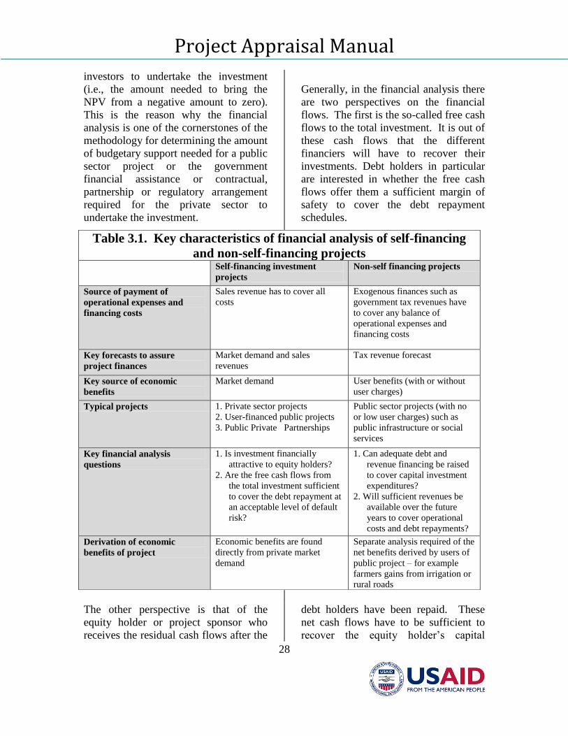
Table 3.1. Key characteristics of financial analysis of self-financing
and non-self-financing projects Self-financing investment
projects
Non-self financing projects
Source of payment of
operational expenses and
financing costs
Sales revenue has to cover all
costs
Exogenous finances such as
government tax revenues have
to cover any balance of
operational expenses and
financing costs
Key forecasts to assure
project finances
Market demand and sales
revenues
Tax revenue forecast
Key source of economic
benefits
Market demand User benefits (with or without
user charges)
Typical projects 1. Private sector projects
2. User-financed public projects
3. Public Private Partnerships
Public sector projects (with no
or low user charges) such as
public infrastructure or social
services
Key financial analysis
questions
1. Is investment financially
attractive to equity holders?
2. Are the free cash flows from
the total investment sufficient
to cover the debt repayment at
an acceptable level of default
risk?
1. Can adequate debt and
revenue financing be raised
to cover capital investment
expenditures?
2. Will sufficient revenues be
available over the future
years to cover operational
costs and debt repayments?
Derivation of economic
benefits of project
Economic benefits are found
directly from private market
demand
Separate analysis required of the
net benefits derived by users of
public project – for example
farmers gains from irrigation or
rural roads
Project Appraisal Manual
29
investment. This perspective is critical
in all private sector projects as well as all
public projects that expect to cover their
costs through user charges or for all
public private partnership arrangements.
In all other non-self-financing projects
with little or no user charges being
collected, the financial viability of the
project depends upon the estimation of
future availability of general public
sector revenues. Table 3.1 is provided
to help sensitise the project analyst to the
different roles of financial analysis for
self-financing and non self-financing
projects.
The building blocks for the financial
analysis of a project are as follows:
Investment Plan
Combines information from the market
and technical analyses to establish a
detailed plan for annual incremental
expected capital expenditures during a
project’s investment phase. Capital
expenditures include expenditures on
land, buildings, machinery, equipment,
building materials, and construction and
management labor.
Should provide estimates of the
liquidation or scrap value of all major
fixed assets and the value of net working
capital at the end of a project’s life.
Should disaggregate expenditures on
machinery, equipment, and building
materials into tradable and non-tradable
commodities.
Should indicate the breakdown of
workers by skill and likely sources of
availability.
Operating Plan
Combines information from the market
and technical analyses to establish a
detailed plan for the operating phase of a
project.
Should provide projections of expected
sales revenues and expected operating
costs for each year during the operating
phase. Operating costs include operating
material inputs and operating labor.
Should forecast annual net working
capital requirements.
Should also specify the management and
operating manpower requirements by
skill and source of availability for each
year of the operating phase.
Should disaggregate material inputs into
tradable and non-tradable commodities.
Financing Plan
Should provide details about how any
anticipated negative net cash flows will
be financed during both the investment
and operating phases of a project.
Equity investors should be identified and
the anticipated timing of their
contributions should be specified;
dividend policy, if any, should also be
stated.
Debt-holders should be identified and
the anticipated timing of their
contributions should be specified;
interest and amortization schedules
should also be stated.
These financial data can be combined in
the manner described to determine
whether a project is financially viable
and attractive to investors.
Financial Attractiveness
There are various criteria that can be
used to judge the financial attractiveness
Project Appraisal Manual
30
of an investment opportunity. These
include the net present value (NPV)
criterion, the internal rate of return (IRR)
criterion, the payback period, and
benefit-cost ratios. The strengths and
weaknesses of these criteria are
reviewed below.
Economic Analysis
The starting-point for the economic
analysis is the expected incremental net
cash flows to total capital from the
financial analysis. When there are
perfectly competitive, undistorted
markets (for closely related
commodities), and there are no other
reasons for economic externalities to
exist, market prices will provide a
reasonable measure of marginal
economic benefits or marginal economic
costs. Under these conditions, and
where a project introduces only small
changes in the demand for its inputs and
in the supply of its outputs, the financial
analysis could serve as a proxy for the
economic analysis.
When these requirements are not
satisfied, however, then market prices no
longer provide a reliable measure of
marginal economic benefits or costs.
The broader perspective taken by the
economic analysis requires that a series
of adjustments be made to convert
estimates of incremental cash receipts
into incremental economic benefits and
estimates of incremental cash
disbursements into incremental
economic costs. These adjustments are
based on Harberger’s three basic
postulates for applied welfare
economics, which can be used to
measure economic benefits and costs
and then to add them up, summarized in
three principles: willingness to pay
represents the project’s benefits, supply
price measures the cost of production,
and “an Iraqi dinar is an Iraqi dinar no
matter who receives it or who pays it.”
The market distortions referred to above
fall into the broad category of
externalities. In a nutshell, these
distortions or externalities comprise of
taxes, subsidies, trade tariffs, price
controls, monopoly markets,
environmental impacts such as pollution
or congestion, and open access or
common property situations. Again, we
come across these externalities in
estimating the price of capital (discount
rate) because of imperfect capital
markets and the price of foreign
exchange because of trade distortions
and controls in the foreign exchange
markets. Similarly, there may be
distortions in the labor market where the
financial wage rate may be different
from the economic price of labor
because of taxes, minimum wage rules
and other imperfections in the labor
market.
In the case of private sector projects or
other self-sustaining projects such as
public sector investments expecting to
recover their costs from user charges
(such as is the case with public private
partnerships), the economic benefits can
be found from the market demand for
the project outputs adjusting for the
externalities in this and related markets.
By contrast, for non-self-sustaining
projects such as a public road, the
economic benefits are all external to the
project financial accounts. Essentially in
such cases a separate financial and
Project Appraisal Manual
31
economic analysis is required of the
benefit derived by the user. This is
commonly done, for example, to
estimate the benefits that farmers may
derive from a new irrigation scheme or
new rural road. This difference is noted
in Table 3.1 above.
The impact of a project on other
industries or sectors is also of
importance to its economic analysis
since industries producing close
complementary or substitute products
may experience demand or supply
changes as a result of a project. In
particular, industries producing close
complements to a project’s output are
likely to experience an increase in
demand whereas those producing close
substitutes are likely to experience a
decrease in demand. If the markets for
these products are also distorted due to
congestion, pollution, taxes, or subsidies
etc., then additional economic
externalities will arise. Also, the cost of
producing these related products could
be affected if a project introduces a
technological innovation that lowers
costs (a technological externality). These
externalities should be incorporated into
the economic analysis of a project.
The economic analysis is a key
determinant of whether a project should
receive government financial assistance.
Only a project with a positive NPV of
incremental net economic benefits
should qualify for approval and/or
financial assistance.
Distributional Analysis
The distributional analysis, also referred
to as stakeholders’ analysis, deals with
income changes that are brought about
as a result of the project. This part of the
analysis asks the following question:
who will benefit from the project and by
how much and who will lose or will pay
for the project and by how much? Both
the financial and economic analyses
have to be completed before the
distributional impacts can be
determined.
This Manual does not attempt to attach
different values to the benefits received
by different income groups. Instead, the
procedure adopted is based on
Harberger’s third basic postulate that
treats a dinar as a dinar no matter to
whom it accrues, and therefore, adds up
the costs and benefits without regard to
which person receive them.
The use of distributional weights could
lead to misleading conclusions and
possibly an artificial re-structuring of the
project. Assigning weights for various
subgroups in the economy could mean
that the attractiveness of the project is
dependent on how it is financed. This
would necessitate not only the analysis
of the project’s incremental benefits and
costs but also of the various tax
increases which could be used to finance
it. Clearly, this would complicate the
evaluation of the project.
A distributional analysis combines a
financial analysis along with the
corresponding externalities affecting
each group. The sum of these analyses
across the various income groups should
add up to the economic analysis of the
overall project. In this way, it is possible
to identify those groups that gain and
those that lose as a result of a project.
Project Appraisal Manual
32
Risk Analysis
Like everyone else, project analysts
simply do not know with certainty what
will happen in the future. Hence, the
forecasts that are used in the market,
technical, financial, economic and
distributional analyses are all made
under conditions of uncertainty. The
prices of inputs and outputs, wages, rate
of inflation, and exchange rate are all
crucial for projecting future cash flows
and it is not known how their values will
vary over the life of the project. As such,
the single valued outcome (NPV, IRR)
of the financial analysis will not be
accurate or meaningful. As the
economic and distributive analyses are
based on the financial cash flows, their
outcomes will also suffer from the same
shortcoming. It is no exaggeration to
say that the only thing known with
certainty about the outcome of project
analysis is that the numbers emerging
from it will never be attained when the
project is actually implemented.
Since many of the parameters are
uncertain, the results of financial,
economic and distributional analyses in
terms of the selection criterion (IRR or
NPV), the cash flows and the
externalities will yield only one of the
several probable values. What is
required is a distribution of values of
these outcomes that incorporate all the
possible values that the various
parameters may assume. When there is
no information about likely probability
distributions of prices and quantities, it
is necessary to make informed guesses
about future values of a project’s
variables. In other cases when some
knowledge of probability distributions is
available, it will be possible to calculate
the expected values of the variables, or
to make projections based on past data
that take account of the historical means
and variances of the variables. The topic
of risk analysis provides the
methodology for dealing with
uncertainty when there is some
knowledge of probability distributions.
To begin with, a sensitivity analysis tells
us which parameters are significant for
the outcome of the project. These
become risk variables. Other parameters
that do not matter much may be ignored.
For each risk variable, a probability
distribution and range of values is
assigned. Correlations among variables
are also built into the model. Finally, a
Monte Carlo simulation is performed
and the model results are analyzed.
What the risk analysis yields is not a
single number but a distribution of
results, such as expected values of the
desired outcomes, the probabilities of
negative returns and the variability of
outcomes. Risk analysis is then extended
to economic and distributive analyses.
The results of the risk analysis enable
the decision makers to make a more
informed decision about project
selection.
To manage risk a way must be found to
redesign or reorganize a project in order
to reallocate risk efficiently. This
requires not simply a cost perspective,
where the aim is to reduce risk to one
party by shifting it on to others - clearly
a zero-sum game - but rather an
efficiency perspective, where with the
right contracts one party can gain
substantially without corresponding

Project Appraisal Manual
33
costs to other parties. The solution is to
reallocate risk to those parties who can
best bear it.

Project Appraisal Manual
34
Chapter IV: Schematic Diagram
Project Appraisal Manual
35
CHAPTER IV: PROJECT EVALUATION DIAGRAM
This schematic diagram of project
evaluation framework is based on a
hypothetical power project.
Basic Facts:
The utility authority of the county
currently operates two dams, and a
thermal power plant (installed capacity
of 912, 160 and 30 MW, respectively).
The utility authority proposes to build a
third dam to meet the increasing
domestic and foreign demand of
electricity on the system. The dam will
be located about 150 km north of a lake.
The expected annual amount of
electricity generated is 1150 GWH. Part
of the energy generated will be exported
to the neighboring countries.
The total project cost (at 1996 price
level) is estimated at 310 million US$.
79% and 21% of the total cost are in
foreign and domestic currency,
respectively.
Foreign component of investment cost is
financed with a subsidized foreign loan.
Tariff rates charged to main domestic
and foreign clients have remained
unchanged for years. Under a
contractual arrangement with foreign
clients, tariff rates are adjusted for
inflation every five years.
Project outcomes:
Under the current tariff policy, the
project is not viable from the financial
viewpoint. The net present values are -
44 and -174 billion in domestic currency
when the utility or an independent power
project undertakes the project
respectively.
Different tariff rates, which take into
account the construction cost of the
hydro plant makes the project financially
viable from the equity holder’s point of
view. It is recommended to negotiate a
faster adjustment of nominal tariffs with
domestic customers.
Project is highly attractive from the
economic point of view (NPV equals to
72 billion of domestic currency), with a
10% probability of negative economic
outcome.
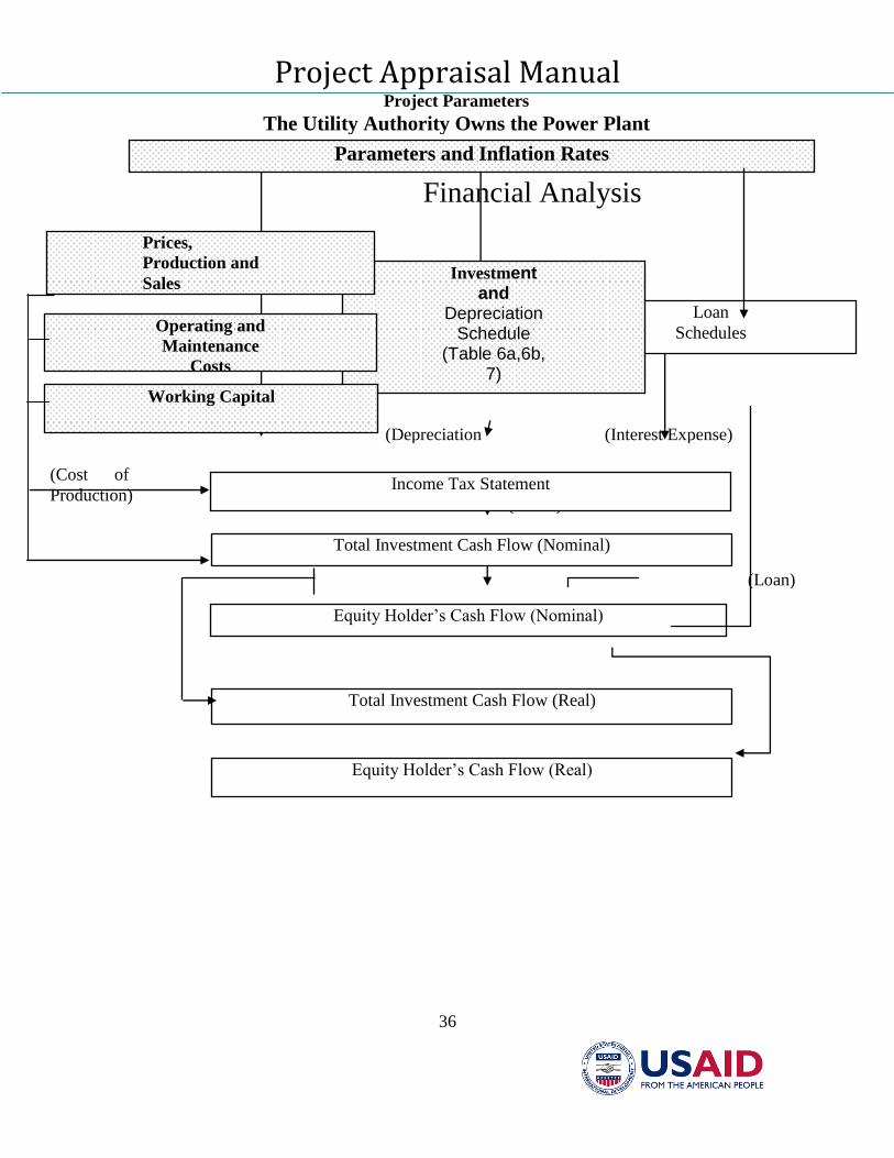
Project Appraisal Manual
36
Parameters and Inflation Rates
Loan
Schedules
Investment and
Depreciation Schedule
(Table 6a,6b, 7)
Equity Holder’s Cash Flow (Nominal)
Total Investment Cash Flow (Real)
Equity Holder’s Cash Flow (Real)
Prices,
Production and
Sales
Operating and
Maintenance
Costs
(Interest Expense) (Depreciation Expense)
(Cost of
Production) (Taxes)
(Loan)
Project Parameters
The Utility Authority Owns the Power Plant
Financial Analysis
Total Investment Cash Flow (Nominal)
Income Tax Statement
Working Capital
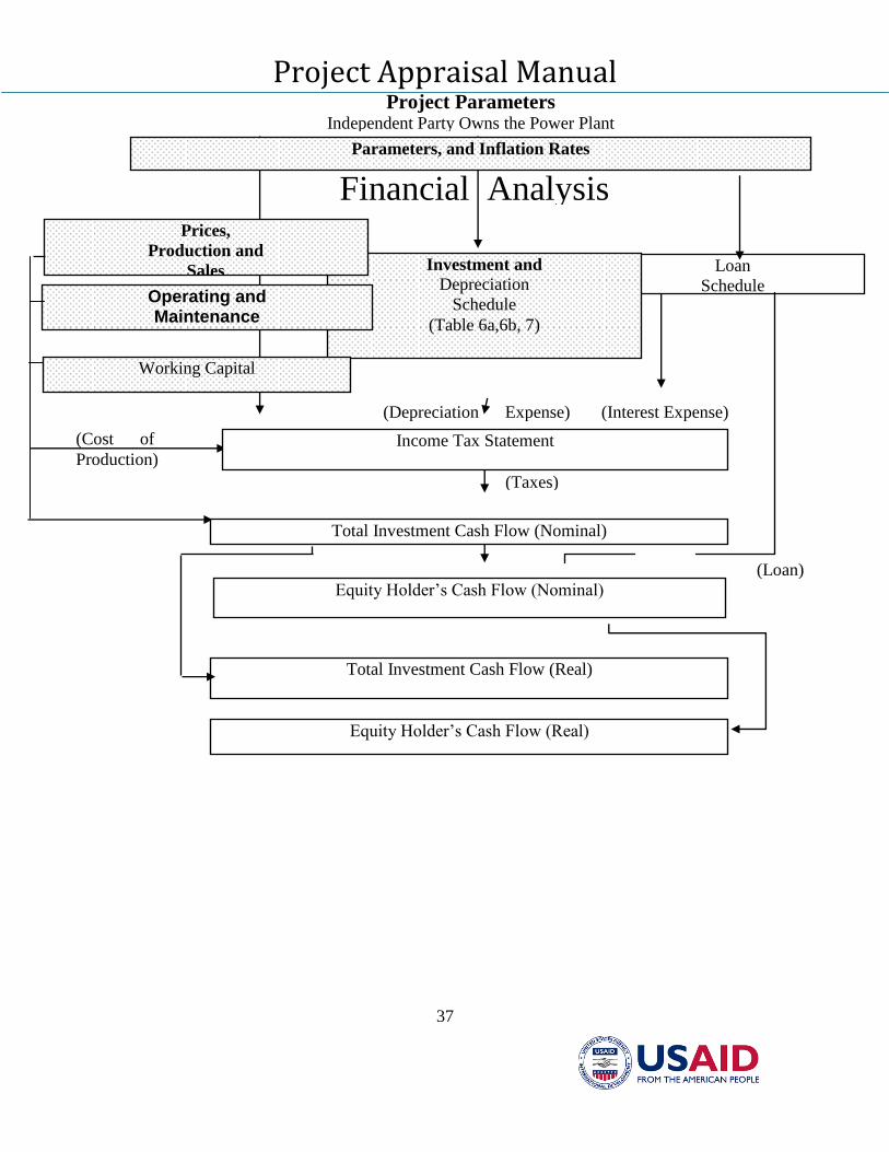
Project Appraisal Manual
37
Parameters, and Inflation Rates
Loan
Schedule
s
Investment and Depreciation
Schedule
(Table 6a,6b, 7)
Equity Holder’s Cash Flow (Nominal)
Total Investment Cash Flow (Real)
Equity Holder’s Cash Flow (Real)
Prices,
Production and
Sales
Operating and Maintenance
Costs
(Interest Expense) (Depreciation Expense)
(Cost of
Production)
(Taxes)
(Loan)
Project Parameters Independent Party Owns the Power Plant
Financial Analysis
Total Investment Cash Flow (Nominal)
Income Tax Statement
Working Capital
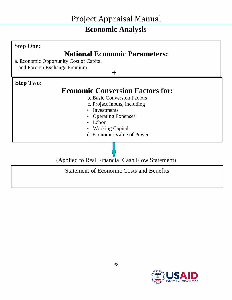
Project Appraisal Manual
38
Economic Analysis
Step One:
National Economic Parameters: a. Economic Opportunity Cost of Capital
and Foreign Exchange Premium +
Step Two:
Economic Conversion Factors for: b. Basic Conversion Factors
c. Project Inputs, including
• Investments
• Operating Expenses
• Labor
• Working Capital
d. Economic Value of Power
Statement of Economic Costs and Benefits
(Applied to Real Financial Cash Flow Statement)
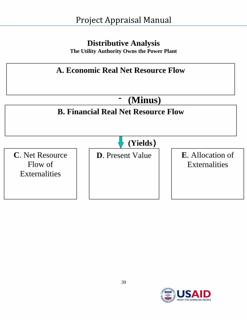
Project Appraisal Manual
39
Distributive Analysis The Utility Authority Owns the Power Plant
A. Economic Real Net Resource Flow
B. Financial Real Net Resource Flow
C. Net Resource
Flow of
Externalities
D. Present Value E. Allocation of
Externalities
- (Minus)
(Yields)
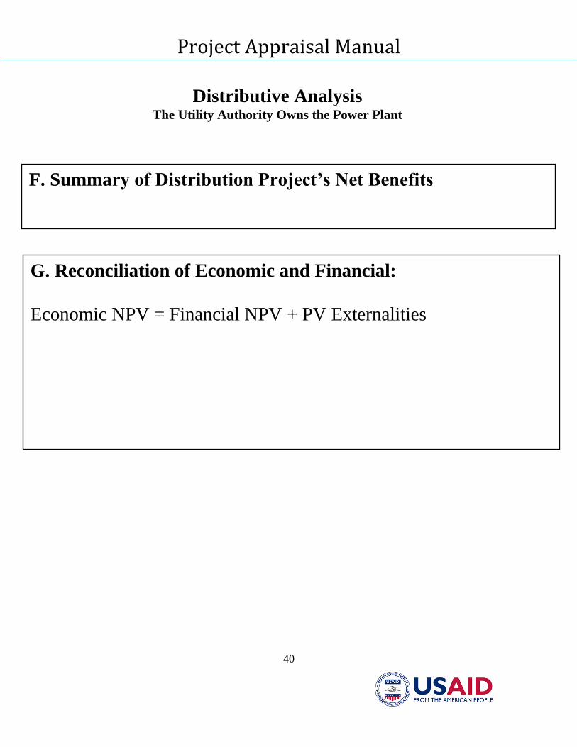
Project Appraisal Manual
40
Distributive Analysis The Utility Authority Owns the Power Plant
F. Summary of Distribution Project’s Net Benefits
G. Reconciliation of Economic and Financial:
Economic NPV = Financial NPV + PV Externalities
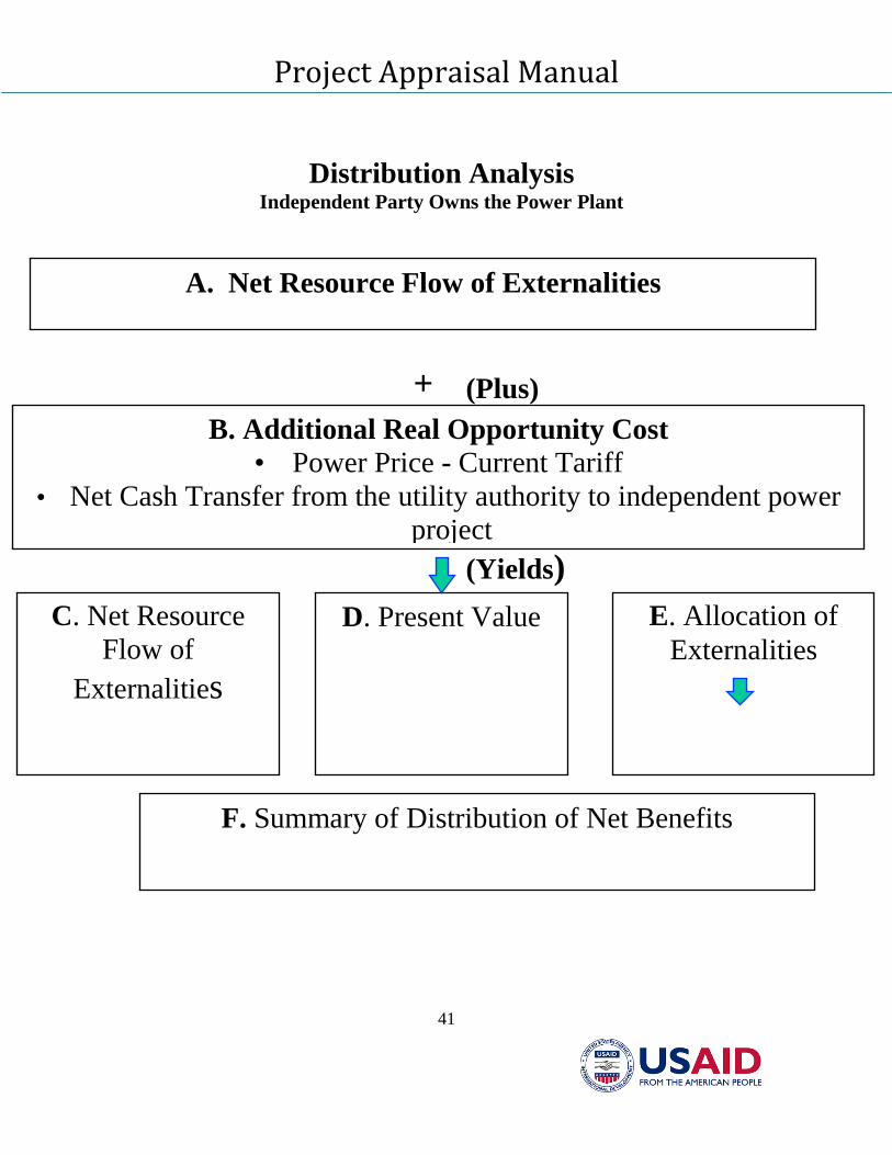
Project Appraisal Manual
41
Distribution Analysis Independent Party Owns the Power Plant
A. Net Resource Flow of Externalities
B. Additional Real Opportunity Cost
• Power Price - Current Tariff
• Net Cash Transfer from the utility authority to independent power
project
C. Net Resource
Flow of
Externalities
D. Present Value E. Allocation of
Externalities
+ (Plus)
(Yields)
F. Summary of Distribution of Net Benefits
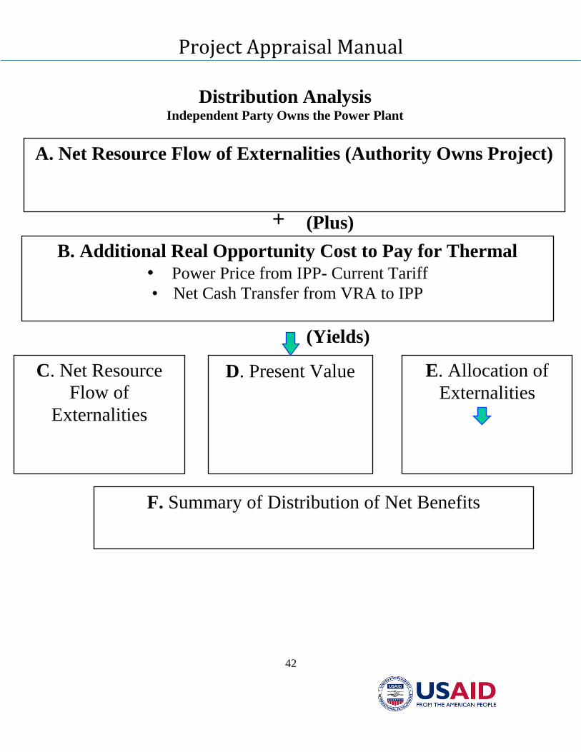
Project Appraisal Manual
42
Distribution Analysis Independent Party Owns the Power Plant
A. Net Resource Flow of Externalities (Authority Owns Project)
B. Additional Real Opportunity Cost to Pay for Thermal
• Power Price from IPP- Current Tariff
• Net Cash Transfer from VRA to IPP
C. Net Resource
Flow of
Externalities
D. Present Value E. Allocation of
Externalities
+ (Plus)
(Yields)
F. Summary of Distribution of Net Benefits
Project Appraisal Manual
43
Risk Analysis
A. Sensitivity Analysis
B. Risk Variables
C. Results
Project Appraisal Manual
44
Chapter V: Project Evaluation Criteria
Project Appraisal Manual
45
CHAPTER V: PROJECT EVALUATION CRITERIA
Introduction
As mentioned in the previous chapter,
the financial attractiveness of a project is
determined by the net present value
(NPV) of its expected incremental net
cash flows and the economic desirability
is measured by the NPV of its
incremental net economic benefits. The
NPV criterion is widely accepted by
accountants, financial analysts, and
economists as the only criterion that
yields correct project choice in all
circumstances. However, some private
investors and public sector agencies
have frequently relied upon other criteria
such as a project’s internal rate of return
(IRR) or a benefit-cost ratio; some have
used a payback period criterion. The
strengths and weaknesses of these
criteria are examined in this chapter in
order to demonstrate why the NPV
criterion is the most reliable one for
government analysts to use.
Time Dimension of a Project
Investment decisions are fundamentally
different from consumption decisions
because the former have a time
dimension. For example, land and
capital equipment are purchased at one
point in time, and they are expected to
generate net cash flows, or net economic
benefits, over a number of subsequent
years. To determine whether the
investment is worthwhile it is necessary
to compare the benefits and costs that
occur in different time periods. The
problem is that a Iraqi dinar
spent/received today is worth more than
an Iraqi dinar spent/received in a later
time period. In other words, it is not
possible just to add up the benefits and
costs of a project to determine which is
larger without first taking account of the
fact that dinars spent on investment
today are worth more today than the
dinars received in benefits in the future.
Expressing the values in terms of either
future or present values can capture the
time dimension of a project’s net cash
flows and net economic benefits. When
moving forward in time to compute
future values, analysts must allow for the
compounding of cash flows. When
bringing future values back to the
present for comparison purposes, it is
necessary to discount them. Discounting
is just the inverse of compounding.
Time Value of Money
Time enhances the value of a dinar today
and reduces the value of a dinar
spent/received in the future. Because
individuals consider waiting before
incurring a cost, it is necessary to
compensate them for forgoing their
consumption today and instead lending
their funds to a bank or a borrower.
Thus, banks and other financial
institutions have to offer interest
payments to the lenders to induce them
to part temporarily with their funds. If
the annual market interest rate were 5%,
then 1 dinar today would be worth 1.05
dinars in a year’s time. This implies that
in equilibrium, lenders value 1.05 dinars
in a year’s time the same as 1 dinar
today.
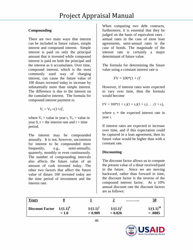
Project Appraisal Manual
46
Compounding
There are two main ways that interest
can be included in future values, simple
interest and compound interest. Simple
interest is paid on only the principal
amount that is invested while compound
interest is paid on both the principal and
the interest as it accumulates. Over time,
compound interest, which is the most
commonly used way of charging
interest, can cause the future value of
100 dinars invested today to increase by
substantially more than simple interest.
The difference is due to the interest on
the cumulative interest. The formula for
compound interest payment is:
Vt = V0 (1+r)t,
where Vt = value in year t, V0 = value in
year 0, r = the interest rate and t = time
period.
The interest may be compounded
annually. It is not, however, uncommon
for interest to be compounded more
frequently, e.g., semi-annually,
quarterly, monthly or even continuously.
The number of compounding intervals
also affects the future value of an
amount of cash invested today. The
other two factors that affect the future
value of dinars 100 invested today are
the time period of investment and the
interest rate.
When comparing two debt contracts,
furthermore, it is essential that they be
judged on the basis of equivalent rates -
annual rates in the case of most loan
agreements, semi-annual rates in the
case of bonds. The magnitude of the
interest rate is certainly a major
determinant of future value.
The formula for determining the future
value using a constant interest rate is
FV = 100*(1 + r)t
However, if interest rates were expected
to vary over time, then the formula
would become
FV = 100*(1 + r1)(1 + r2)(1 + r3) . . . (1 + rt),
where ri = the expected interest rate in
year i.
If interest rates are expected to increase
over time, and if this expectation could
be captured in a loan agreement, then its
future value would be higher than with a
constant rate.
Discounting
The discount factor allows us to compute
the present value of a dinar received/paid
in the future. Since we are moving
backward, rather than forward in time,
the discount factor is the inverse of the
compound interest factor. At a 10%
annual discount rate the discount factors
are as follows:
Years 0 1 2 ……….. 50
Discount Factor 1/(1.1)0 1/(1.1)
1 1/(1.1)
2 1/(1.1)
50
= 1.0 = 0.909 = 0.826 = .0085
Project Appraisal Manual
47
The later a cash flow is received or paid,
the lower its present value. Thus, 100
dinars received 50 years from now has a
value of only dinars 0.85 today at a
discount rate of 10%.
The magnitude of the discount factor is
affected by the same variables as those
that determine the magnitude of the
compound interest factors. One is the
compounding interval.
The annual discount factor is V0 =
Vt/(1+r)t = Vt(1 + r)
-t.
The continuous discount factor is
V0 = Vt/ert = Vt(e
-rt), which is a
smaller number.
Besides the timing of the cash flow, the
other factor that determines the discount
rate is the level of market interest rates.
This is why it is critical to pay careful
attention to the estimation of the private
and economic discount rates in the
financial and economic analyses.
The present value can also be interpreted
as the amount that would have to be set
aside today in order to have $100 at a
future date. This is evident from taking
the future value of the present value.
The Net Present Value (NPV)
Criterion
The net present value (NPV) is the
algebraic sum of the present values of
the expected incremental positive and
negative net cash flows over a project’s
anticipated lifetime. If this sum is equal
to zero, then investors can expect to
recover their incremental investment and
earn a rate of return on their capital
equal to the private discount rate used to
compute the present values.7 However,
if the private discount rate is based on
the market cost of capital for a project of
equivalent risk, as it should be, then
investors would be no further ahead with
a zero-NPV project than they would
have been if they had left the funds in
the capital market. Investors are not
worse off; they are just not better off.
A NPV greater than zero means that
investors can expect not only to recover
their capital investment and earn a rate
of return equal to the discount rate, but
also to receive an addition to their real
net worth equal to the positive amount of
the NPV. In other words, a positive-
NPV project outperforms the capital
market and makes investors better off.
Finally, if the NPV is less than zero, then
investors cannot expect to earn a rate of
return equal to the discount rate, nor
possibly to recover their invested capital,
and hence, their real net worth is
expected to decrease. Only projects with
positive NPVs are going to be beneficial
and hence attractive to private investors.
They are unlikely to pursue a project
with a negative NPV unless there are
strategic reasons or they receive
financial assistance.
7 The recovery of the invested capital is
anticipated when NPV 0 because the
incremental capital expenditures are included in
the initial negative net cash flows.
Project Appraisal Manual
48
The formula for computing the NPV of
expected incremental net cash flows
over n time periods with annual
discounting is:
n
ttr
tC
NPV
0 )1(
where the incremental net cash flows
(Ci) could be negative, zero, or positive,
and r is the discount rate equal to the
cost of capital and the sigma sign ( ) is
the symbol for summation. It is today’s
cost of capital that matters because that
is what it either costs to raise the funds
or is being forgone as a result of using
available funds for a project rather than
putting them to work in the capital
market.
The NPV formula for the annual net
cash flow can be written out in its
component present values as follows:
)1(
... + )r + (1
C +
r + 1
C + C = NPV
2
21O nr
nC
The net present value criterion can be
stated in the form of a set of decision
rules.
Decision Rule 1: Do not accept any project unless it generates
a positive NPV when discounted by a
discount rate equal to the opportunity cost
of funds.
Decision Rule 2: To maximize net worth, choose among the
various projects, or scenarios of projects,
the one with the highest NPV. If
investment is subject to a budget
constraint, then choose the package of
projects that maximizes the NPV of the
fixed budget.
Decision Rule 3: When there is no budget constraint and when
a choice must be made between two or
more mutually exclusive projects, e.g.,
projects being considered for the same
building site, then investors who seek to
maximize net worth should select the
project with the highest NPV.
Rule 3 is stated in terms of the absolute
value of the NPV, not in terms of the
NPV per dinar of investment. For
example, consider two projects, A and
B, which are mutually exclusive for
technical reasons and have the following
characteristics:
Project A: NPV of project A
= Dinars 700,000
Present value of
capital expenditure = Dinars 4,000,000.
Project B: NPV of project B
= Dinars 600,000
Present value of
capital expenditure = Dinars 1,500,000.
According to Rule 3, Project A with an
overall NPV of Dinars 700,000 should
be chosen because it has the higher
NPV, even though the NPV per dinar of
investment is higher for Project B (0.4)
than for Project A (0.175). The reason
for choosing Project A is that even
though it requires an incremental
investment of Dinars 2,500,000, it yields
an incremental gain in NPV of Dinars
100,000 over and above a rate of return
equal to the discount rate on the
incremental investment. By choosing
Project B, an investor would have a NPV
of Dinars 600,000, and any additional
Project Appraisal Manual
49
funds are assumed to be invested in the
capital market where they would have a
zero NPV. Thus, by choosing Project A,
an investor would be Dinars 100,000
better off, and Project A is the preferred
choice.
Note that even though the NPV of the
incremental net cash flows might be
negative and a project would not appear
attractive to private investors, it may
create benefits for others in the form of
economic externalities that should be
captured in an economic analysis. If the
economic benefits are sufficiently large
to outweigh the economic costs, then the
government, on the grounds of
improving economic efficiency, would
have reason to offer the private investors
some financial assistance to make the
project more attractive to them.
Investment projects can exhibit different
time profiles for the expected
incremental net cash flow either to total
or equity capital over a project’s life.
For example, the figure below shows
time profiles for three types of
investment projects, namely:
(a) T
he investment expenditures initially
cause the net cash flow to be negative,
but once the expenditure is incurred the
rest of the net cash flows are expected to
be positive over the project’s life.
(b) T
his profile is slightly different because
after a few years of operations, the
replacement of some of the project’s
machinery and equipment causes the net
cash flow to become temporarily
negative.
(c) T
he last profile also turns negative, but in
this case it is due to a major expenditure
at the end of a project, e.g.,
environmental regulations require a
strip-mining site to be restored to its
original condition. The criterion used to
appraise investment projects must be
applicable to any time profile of net cash
flows. Unlike other possible criteria, the
net present value criterion is the only
one that meets this requirement.
Although the NPV criterion is used by
large companies and by government
agencies, they also use alternative
criteria. Each of these alternatives has
serious drawbacks compared to the NPV
criterion and is therefore judged not only
less reliable, but potentially misleading.
When two or more criteria are used to
appraise a project, there is always a
chance that they will point to different
conclusions, and a wrong decision could
be made. This simply creates
unnecessary confusion and possibly
mistakes.
A government project analyst should be
familiar with the shortcomings of these
alternative criteria. Representatives of a
government-owned and controlled
corporation or a private company can
often be quite adamant about the
efficacy of their criteria as a basis for
investment decisions. Although it is not
necessary to tell these financial
managers how to make decisions,
nevertheless when a government project
analyst wants to measure the gain to
private investors from undertaking a
project, then the NPV criterion should be
employed.
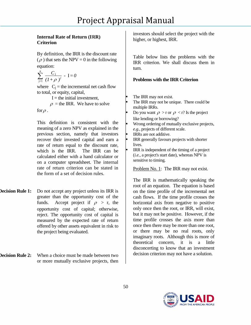
Project Appraisal Manual
50
Internal Rate of Return (IRR)
Criterion
By definition, the IRR is the discount rate
( ) that sets the NPV = 0 in the following
equation:
0 = - ) + (1
C
jI
jn
=1j
where Cj = the incremental net cash flow
to total, or equity, capital,
I = the initial investment,
= the IRR. We have to solve
for .
This definition is consistent with the
meaning of a zero NPV as explained in the
previous section, namely that investors
recover their invested capital and earn a
rate of return equal to the discount rate,
which is the IRR. The IRR can be
calculated either with a hand calculator or
on a computer spreadsheet. The internal
rate of return criterion can be stated in
the form of a set of decision rules.
Decision Rule 1: Do not accept any project unless its IRR is
greater than the opportunity cost of the
funds. Accept project if > r, the
opportunity cost of capital; otherwise,
reject. The opportunity cost of capital is
measured by the expected rate of return
offered by other assets equivalent in risk to
the project being evaluated.
Decision Rule 2: When a choice must be made between two
or more mutually exclusive projects, then
investors should select the project with the
higher, or highest, IRR.
Table below lists the problems with the
IRR criterion. We shall discuss them in
turn.
Problems with the IRR Criterion
The IRR may not exist.
The IRR may not be unique. There could be
multiple IRRs.
Do you want > r or < r? Is the project
like lending or borrowing?
Wrong ordering of mutually exclusive projects,
e.g., projects of different scale.
IRRs are not additive.
IRR generally favours projects with shorter
lives.
IRR is independent of the timing of a project
(i.e., a project's start date), whereas NPV is
sensitive to timing.
Problem No. 1: The IRR may not exist.
The IRR is mathematically speaking the
root of an equation. The equation is based
on the time profile of the incremental net
cash flows. If the time profile crosses the
horizontal axis from negative to positive
only once then the root, or IRR, will exist,
but it may not be positive. However, if the
time profile crosses the axis more than
once then there may be more than one root,
or there may be no real roots, only
imaginary roots. Although this is more of
theoretical concern, it is a little
disconcerting to know that an investment
decision criterion may not have a solution.
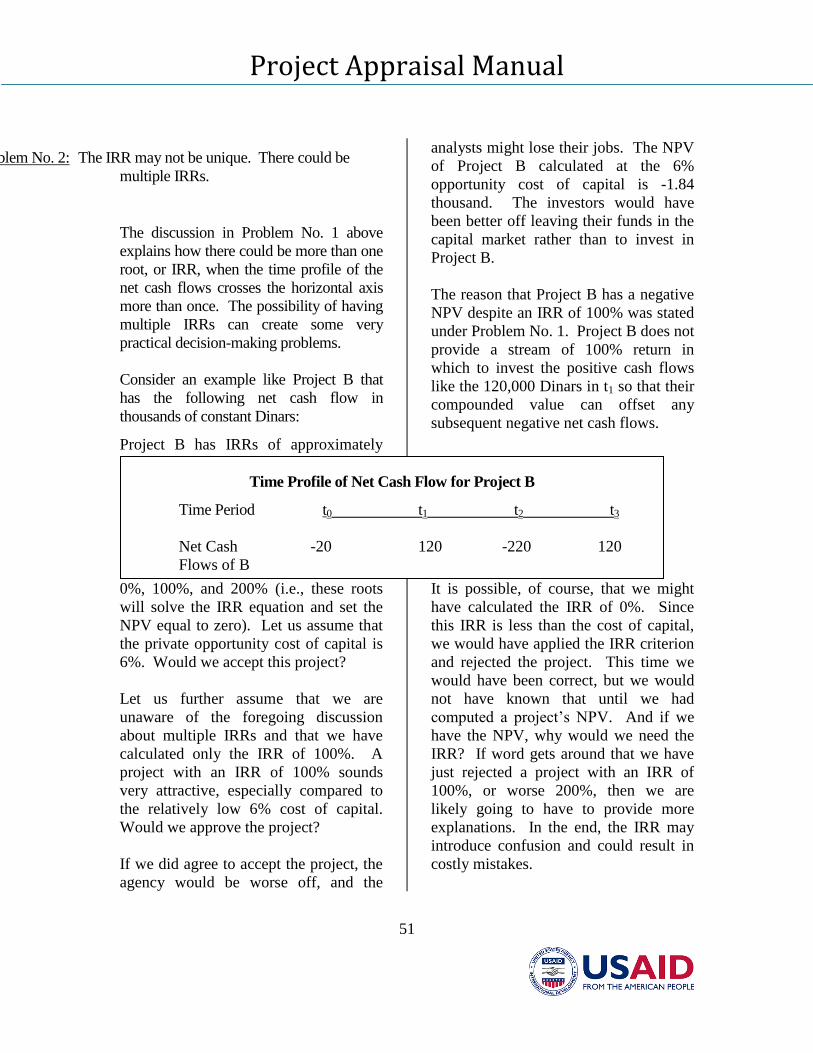
Project Appraisal Manual
51
Problem No. 2: The IRR may not be unique. There could be
multiple IRRs.
The discussion in Problem No. 1 above
explains how there could be more than one
root, or IRR, when the time profile of the
net cash flows crosses the horizontal axis
more than once. The possibility of having
multiple IRRs can create some very
practical decision-making problems.
Consider an example like Project B that
has the following net cash flow in
thousands of constant Dinars:
Project B has IRRs of approximately
0%, 100%, and 200% (i.e., these roots
will solve the IRR equation and set the
NPV equal to zero). Let us assume that
the private opportunity cost of capital is
6%. Would we accept this project?
Let us further assume that we are
unaware of the foregoing discussion
about multiple IRRs and that we have
calculated only the IRR of 100%. A
project with an IRR of 100% sounds
very attractive, especially compared to
the relatively low 6% cost of capital.
Would we approve the project?
If we did agree to accept the project, the
agency would be worse off, and the
analysts might lose their jobs. The NPV
of Project B calculated at the 6%
opportunity cost of capital is -1.84
thousand. The investors would have
been better off leaving their funds in the
capital market rather than to invest in
Project B.
The reason that Project B has a negative
NPV despite an IRR of 100% was stated
under Problem No. 1. Project B does not
provide a stream of 100% return in
which to invest the positive cash flows
like the 120,000 Dinars in t1 so that their
compounded value can offset any
subsequent negative net cash flows.
It is possible, of course, that we might
have calculated the IRR of 0%. Since
this IRR is less than the cost of capital,
we would have applied the IRR criterion
and rejected the project. This time we
would have been correct, but we would
not have known that until we had
computed a project’s NPV. And if we
have the NPV, why would we need the
IRR? If word gets around that we have
just rejected a project with an IRR of
100%, or worse 200%, then we are
likely going to have to provide more
explanations. In the end, the IRR may
introduce confusion and could result in
costly mistakes.
Time Profile of Net Cash Flow for Project B
Time Period t0 t1 t2 t3
Net Cash -20 120 -220 120
Flows of B
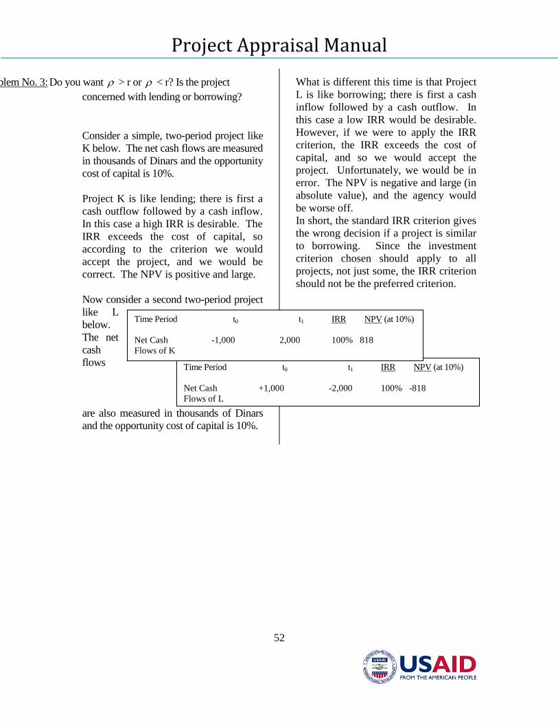
Project Appraisal Manual
52
Problem No. 3: Do you want > r or < r? Is the project
concerned with lending or borrowing?
Consider a simple, two-period project like
K below. The net cash flows are measured
in thousands of Dinars and the opportunity
cost of capital is 10%.
Project K is like lending; there is first a
cash outflow followed by a cash inflow.
In this case a high IRR is desirable. The
IRR exceeds the cost of capital, so
according to the criterion we would
accept the project, and we would be
correct. The NPV is positive and large.
Now consider a second two-period project
like L
below.
The net
cash
flows
are also measured in thousands of Dinars
and the opportunity cost of capital is 10%.
What is different this time is that Project
L is like borrowing; there is first a cash
inflow followed by a cash outflow. In
this case a low IRR would be desirable.
However, if we were to apply the IRR
criterion, the IRR exceeds the cost of
capital, and so we would accept the
project. Unfortunately, we would be in
error. The NPV is negative and large (in
absolute value), and the agency would
be worse off.
In short, the standard IRR criterion gives
the wrong decision if a project is similar
to borrowing. Since the investment
criterion chosen should apply to all
projects, not just some, the IRR criterion
should not be the preferred criterion.
Time Period t0 t1 IRR NPV (at 10%)
Net Cash +1,000 -2,000 100% -818
Flows of L
Time Period t0 t1 IRR NPV (at 10%)
Net Cash -1,000 2,000 100% 818
Flows of K
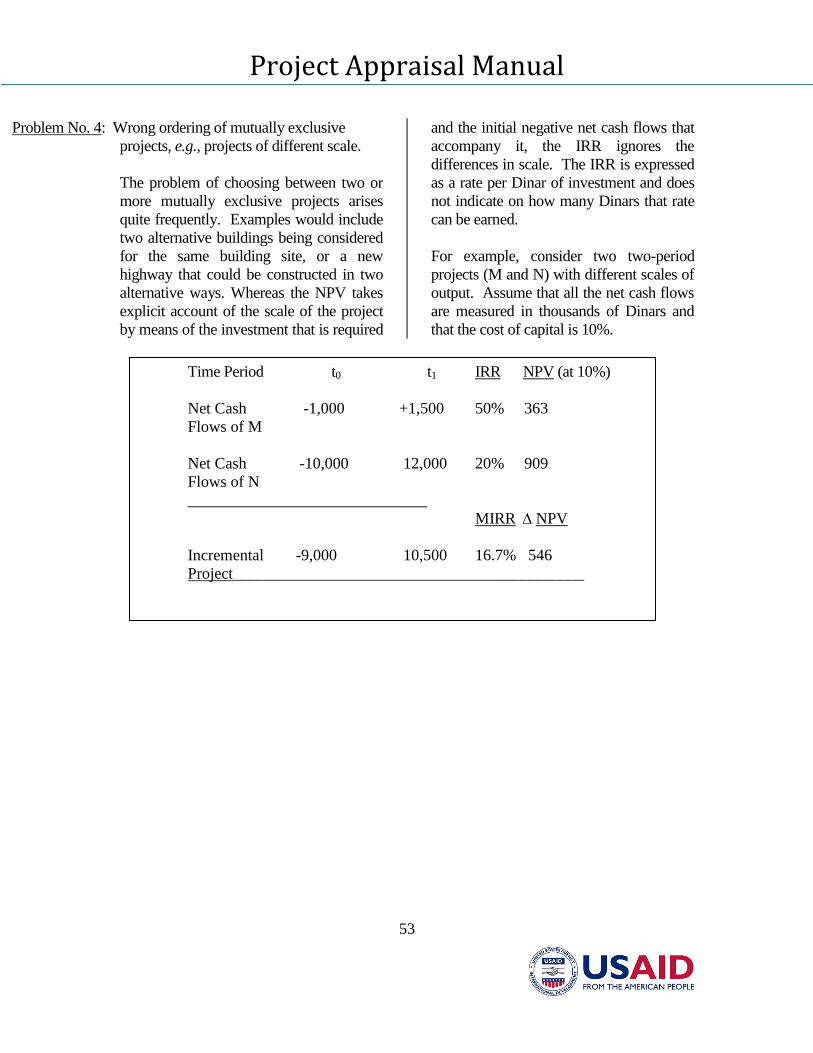
Project Appraisal Manual
53
Problem No. 4: Wrong ordering of mutually exclusive
projects, e.g., projects of different scale.
The problem of choosing between two or
more mutually exclusive projects arises
quite frequently. Examples would include
two alternative buildings being considered
for the same building site, or a new
highway that could be constructed in two
alternative ways. Whereas the NPV takes
explicit account of the scale of the project
by means of the investment that is required
and the initial negative net cash flows that
accompany it, the IRR ignores the
differences in scale. The IRR is expressed
as a rate per Dinar of investment and does
not indicate on how many Dinars that rate
can be earned.
For example, consider two two-period
projects (M and N) with different scales of
output. Assume that all the net cash flows
are measured in thousands of Dinars and
that the cost of capital is 10%.
Time Period t0 t1 IRR NPV (at 10%)
Net Cash -1,000 +1,500 50% 363
Flows of M
Net Cash -10,000 12,000 20% 909
Flows of N
______________________________
MIRR NPV
Incremental -9,000 10,500 16.7% 546
Project____________________________________________
Project Appraisal Manual
54
If Decision Rule 2 of the IRR criterion
were applied, then we would choose the
project with the higher IRR. In this case
that would be Project M. Once again,
however, this would be a mistake. The
NPV of Project N is Dinars 546
thousand higher.
The problem is that with Project M the
rate of return is higher, but it is earned
on only an investment of Dinars 1,000
whereas with Project N, the rate of
return is lower, but the Dinar return is
higher; hence the higher NPV.
Another way to view this problem is to
think about how by accepting Project M,
the remaining Dinars 9,000 is going to
be invested. Lacking anything more
concrete, it is best to assume that the
Dinars 9,000 is invested in the capital
market, where it would have a 10% rate
of return and a NPV of zero. If instead
the Dinars 9,000 were invested in
Project N, there would be an additional
net benefit of Dinars 546,000 over and
above the 10% market return. Clearly,
Project N is the better alternative. This
is also indicated by the marginal internal
rate of return (MIRR) on the incremental
investment of 16.7% which is greater
than the cost of capital.
Problem No. 5: IRRs are not additive.
Larger projects will frequently have a
number of separable components. Each of
these components should be analyzed on
its own merits and then assessed in
conjunction with the other components.
Since some of the possible components
may be mutually exclusive, those separate
combinations have to be examined as well.
Take, for example, a larger three-period
Project T that has two mutually exclusive
projects, 1 and 2, and a third project 3 that
has independent net cash flows, but that
could be undertaken with either one of the
other two. The question is which is the
best package? In the table below, all the
net cash flows are expressed in thousands
of Dinar and the cost of capital is 10%; all
of the separate projects have the same
scale of investment.
Our objective is to maximize the NPV of
Project T. The question is whether that
will occur if we rely on the IRR criterion.
According to the latter, Project 3 is the
most attractive of the individual projects,
and it remains the most attractive even
after assessing it in combination with the
other two. Hence, based on IRR Decision
Rule No. 2, we would select Project 3 by
itself.
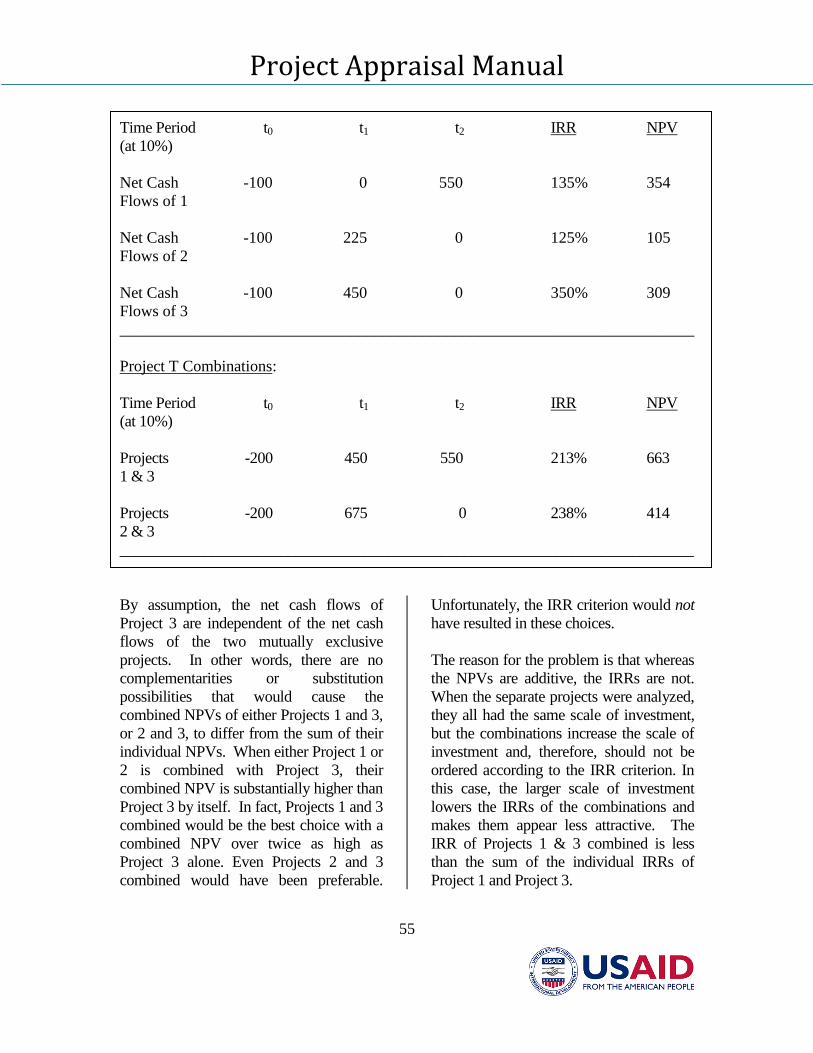
Project Appraisal Manual
55
Time Period t0 t1 t2 IRR NPV
(at 10%)
Net Cash -100 0 550 135% 354
Flows of 1
Net Cash -100 225 0 125% 105
Flows of 2
Net Cash -100 450 0 350% 309
Flows of 3
________________________________________________________________________
Project T Combinations:
Time Period t0 t1 t2 IRR NPV
(at 10%)
Projects -200 450 550 213% 663
1 & 3
Projects -200 675 0 238% 414
2 & 3
___________________________________________________________________________
By assumption, the net cash flows of
Project 3 are independent of the net cash
flows of the two mutually exclusive
projects. In other words, there are no
complementarities or substitution
possibilities that would cause the
combined NPVs of either Projects 1 and 3,
or 2 and 3, to differ from the sum of their
individual NPVs. When either Project 1 or
2 is combined with Project 3, their
combined NPV is substantially higher than
Project 3 by itself. In fact, Projects 1 and 3
combined would be the best choice with a
combined NPV over twice as high as
Project 3 alone. Even Projects 2 and 3
combined would have been preferable.
Unfortunately, the IRR criterion would not
have resulted in these choices.
The reason for the problem is that whereas
the NPVs are additive, the IRRs are not.
When the separate projects were analyzed,
they all had the same scale of investment,
but the combinations increase the scale of
investment and, therefore, should not be
ordered according to the IRR criterion. In
this case, the larger scale of investment
lowers the IRRs of the combinations and
makes them appear less attractive. The
IRR of Projects 1 & 3 combined is less
than the sum of the individual IRRs of
Project 1 and Project 3.
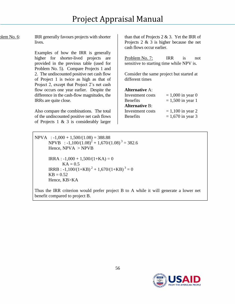
Project Appraisal Manual
56
Problem No. 6: IRR generally favours projects with shorter
lives.
Examples of how the IRR is generally
higher for shorter-lived projects are
provided in the previous table (used for
Problem No. 5). Compare Projects 1 and
2. The undiscounted positive net cash flow
of Project 1 is twice as high as that of
Project 2, except that Project 2’s net cash
flow occurs one year earlier. Despite the
difference in the cash-flow magnitudes, the
IRRs are quite close.
Also compare the combinations. The total
of the undiscounted positive net cash flows
of Projects 1 & 3 is considerably larger
than that of Projects 2 & 3. Yet the IRR of
Projects 2 & 3 is higher because the net
cash flows occur earlier.
Problem No. 7: IRR is not
sensitive to starting time while NPV is.
Consider the same project but started at
different times
Alternative A:
Investment costs = 1,000 in year 0
Benefits = 1,500 in year 1
Alternative B:
Investment costs = 1,100 in year 2
Benefits = 1,670 in year 3
NPVA : -1,000 + 1,500/(1.08) = 388.88
NPVB : -1,100/(1.08)2 + 1,670/(1.08)
3 = 382.6
Hence, NPVA > NPVB
IRRA : -1,000 + 1,500/(1+KA) = 0
KA = 0.5
IRRB : -1,100/(1+KB) 2
+ 1,670/(1+KB) 3
= 0
KB = 0.52
Hence, KB>KA
Thus the IRR criterion would prefer project B to A while it will generate a lower net
benefit compared to project B.
Project Appraisal Manual
57
)(
)(
CostsorEconomicshOutlowsNPVofNetCa
BenefitsorEconomicshInflowsNPVofNetCaBCR
Benefit-Cost Ratio (BCR) Criterion
As its name indicates, the benefit-cost
ratio, or what is sometimes referred to as
the profitability index, is the ratio of the
NPV of the net cash inflows (or
economic benefits) to the NPV of the net
cash outflows (or economic costs):
The benefit-cost ratio criterion can be
stated in the form of a set of decision
rules.
The BCR Criterion
Decision Rule 1: Do not accept any project unless its BCR
is greater than one. Accept project if BCR
> 1; otherwise, reject. The NPVs in both
the numerator and the denominator of the
ratio should be discounted by the
opportunity cost of the funds. The
opportunity cost of capital is measured by
the expected rate of return offered by other
assets equivalent in risk to the project
being evaluated.
Decision Rule 2: When a choice must be made between two
or more mutually exclusive projects, then
investors should select the project with the
higher, or highest, BCR.
Many government agencies around the middle-
east (MENA) started using the NPV criterion
as the main basis for decision-making in the
economic analysis of a project, but they have in
the past used the BCR and the Economic IRR
as indicators of economic desirability. To use
the BCR as a measure of financial or economic
desirability runs the risk of screening out
possible candidate projects
according to a faulty criterion. In
some instances, worthy
candidates could be eliminated
from consideration early on based
on their BCRs, and in so doing the overall
NPV could be lowered unnecessarily. As
illustrated below, furthermore, the NPV
criterion and the BCR criterion can often draw
the opposite conclusion. Using the two criteria
together then becomes a source of confusion,
and possibly mistakes.
Although the BCR is popular because it is a
handy rule-of-thumb and summary statistic, it
does have two major weaknesses, as discussed
below:
Problem No. 1: The BCR is sensitive to the
definition of costs. Problem of recurring
capital costs.
When a project profile is drawn, it is not
uncommon to have negative net cash flows in
some years during the project’s life. The
question is should these periodic negative net
cash flows be included in the capital costs in
the denominator or should they be counted as
net cash flows (albeit negative) in the
numerator. The problem is that the BCR is a
ratio. Whereas multiplying or dividing the
numerator and denominator of a ratio by the
same number does not alter
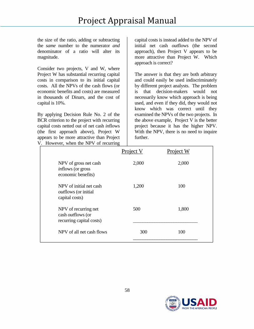
Project Appraisal Manual
58
the size of the ratio, adding or subtracting
the same number to the numerator and
denominator of a ratio will alter its
magnitude.
Consider two projects, V and W, where
Project W has substantial recurring capital
costs in comparison to its initial capital
costs. All the NPVs of the cash flows (or
economic benefits and costs) are measured
in thousands of Dinars, and the cost of
capital is 10%.
By applying Decision Rule No. 2 of the
BCR criterion to the project with recurring
capital costs netted out of net cash inflows
(the first approach above), Project W
appears to be more attractive than Project
V. However, when the NPV of recurring
capital costs is instead added to the NPV of
initial net cash outflows (the second
approach), then Project V appears to be
more attractive than Project W. Which
approach is correct?
The answer is that they are both arbitrary
and could easily be used indiscriminately
by different project analysts. The problem
is that decision-makers would not
necessarily know which approach is being
used, and even if they did, they would not
know which was correct until they
examined the NPVs of the two projects. In
the above example, Project V is the better
project because it has the higher NPV.
With the NPV, there is no need to inquire
further.
Project V Project W
NPV of gross net cash 2,000 2,000
inflows (or gross
economic benefits)
NPV of initial net cash 1,200 100
outflows (or initial
capital costs)
NPV of recurring net 500 1,800
cash outflows (or
recurring capital costs) ___________________________
NPV of all net cash flows 300 100
___________________________
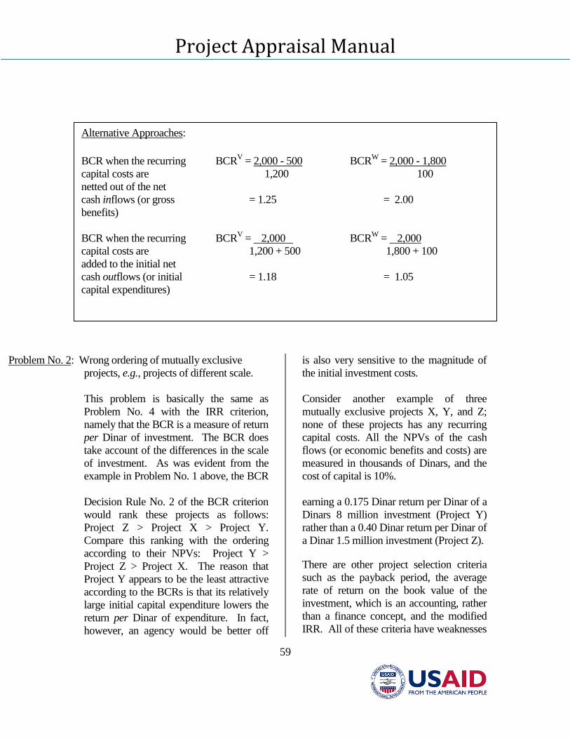
Project Appraisal Manual
59
Problem No. 2: Wrong ordering of mutually exclusive
projects, e.g., projects of different scale.
This problem is basically the same as
Problem No. 4 with the IRR criterion,
namely that the BCR is a measure of return
per Dinar of investment. The BCR does
take account of the differences in the scale
of investment. As was evident from the
example in Problem No. 1 above, the BCR
is also very sensitive to the magnitude of
the initial investment costs.
Consider another example of three
mutually exclusive projects X, Y, and Z;
none of these projects has any recurring
capital costs. All the NPVs of the cash
flows (or economic benefits and costs) are
measured in thousands of Dinars, and the
cost of capital is 10%.
Decision Rule No. 2 of the BCR criterion
would rank these projects as follows:
Project Z > Project X > Project Y.
Compare this ranking with the ordering
according to their NPVs: Project Y >
Project Z > Project X. The reason that
Project Y appears to be the least attractive
according to the BCRs is that its relatively
large initial capital expenditure lowers the
return per Dinar of expenditure. In fact,
however, an agency would be better off
earning a 0.175 Dinar return per Dinar of a
Dinars 8 million investment (Project Y)
rather than a 0.40 Dinar return per Dinar of
a Dinar 1.5 million investment (Project Z).
There are other project selection criteria
such as the payback period, the average
rate of return on the book value of the
investment, which is an accounting, rather
than a finance concept, and the modified
IRR. All of these criteria have weaknesses
Alternative Approaches:
BCR when the recurring BCR
V = 2,000 - 500 BCR
W = 2,000 - 1,800
capital costs are 1,200 100
netted out of the net
cash inflows (or gross = 1.25 = 2.00
benefits)
BCR when the recurring BCRV = 2,000 BCR
W = 2,000
capital costs are 1,200 + 500 1,800 + 100
added to the initial net
cash outflows (or initial = 1.18 = 1.05
capital expenditures)
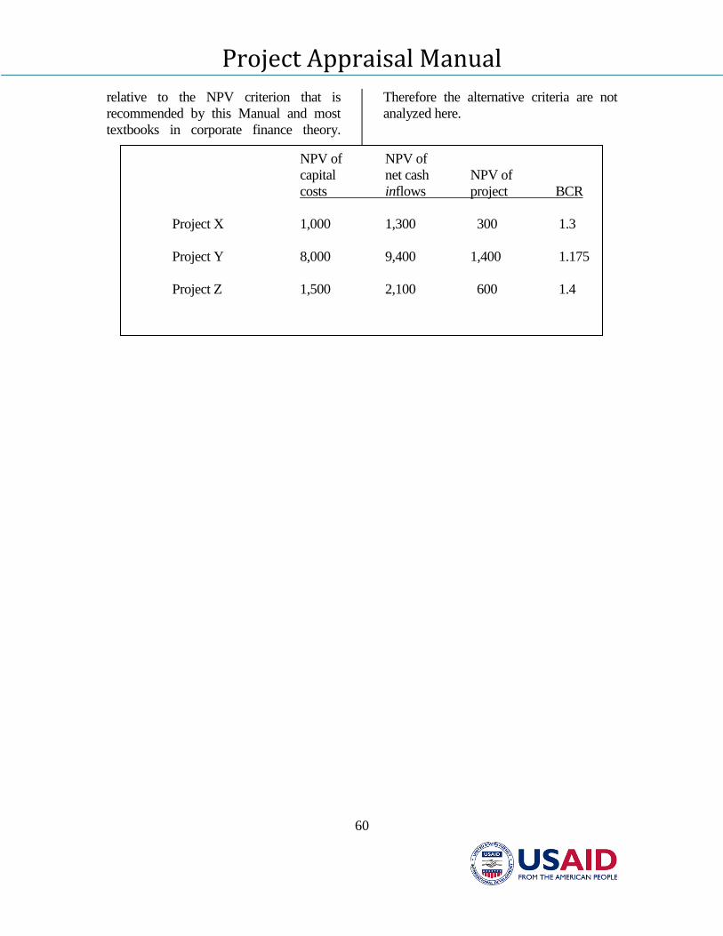
Project Appraisal Manual
60
relative to the NPV criterion that is
recommended by this Manual and most
textbooks in corporate finance theory.
Therefore the alternative criteria are not
analyzed here.
NPV of NPV of
capital net cash NPV of
costs inflows project BCR
Project X 1,000 1,300 300 1.3
Project Y 8,000 9,400 1,400 1.175
Project Z 1,500 2,100 600 1.4
Project Appraisal Manual
61
Chapter VI: Financial Analysis of a Project
Project Appraisal Manual
62
CHAPTER VI: THE FINANCIAL ANALYSIS OF A PROJECT
Introduction
The financial analysis of a project helps
determine the financial sustainability of
the project and its overall success. In its
simplest form, one can describe the
financial analysis of a project as a
process that entails the organization of
specific data requirements in certain
statements, followed by the application
of certain investment criteria to these
statements to determine the financial
profitability or sustainability of the
project. This process requires an
understanding of the concepts, principles
and common conventions that underlie a
correct financial appraisal. Moreover,
the understanding of these concepts and
principles is important in defining the
data requirements for conducting the
financial appraisal of the project.
This chapter presents the concepts and
principles that are necessary to use the
data in constructing financial profiles for
the project’s receipts and expenditures
over the project’s life. These financial
profiles are known as the project’s cash
flow statements.8
8 The cash flow statement is the main financial
statement used to assess a project’s viability.
Other financial statements may be also used to
assess a project’s viability but play different
roles. The statement of profit and loss, for
example, helps determine a project’s net income,
and subsequent tax liability, following the
accounting rules. Unlike the cash flow
statement, the income statement is not concerned
with actual cash inflows that pay dividends and
outflows that finance expenditures, and help
determine the value of the project. Also, the
balance sheet and the statement of sources and
applications of funds cannot alone determine the
viability of a project.
The chapter is largely a “hands-on”
chapter. It presents the concepts and
principles underlying a financial
analysis, provides illustrations for most
of these concepts and offers practical
guidelines for the actual construction of
a financial cash flow statement and the
analysis of these statements. While the
bulk of the chapter deals with the nuts
and bolts of a financial analysis, several
annexes provide additional information.
Why a financial appraisal for a public
sector project?
It may appear that the financial appraisal
of a project is only of interest to a
private investor who wishes to determine
the net financial gain (or loss) resulting
from a project. From a country’s point
of view, a project will increase the
country’s net wealth if it has net positive
economic returns. Conversely a project
that yields negative economic returns
should not be undertaken as it would
lower the net wealth of society as a
whole. Consequently, one may expect
the emphasis of the appraisal of
government projects to be on the
economic analysis of projects only.
Indeed, when appraising projects in the
1960s and 1970s, the emphasis of
development institutions was on the
economic appraisal only. Why then do
we need to conduct the financial
appraisal of a public-sector project in
addition to its economic analysis and
why is more attention being paid to the
financial analysis now than in the 1960s
and 1970s?
Project Appraisal Manual
63
Financial Sustainability
There are several reasons to conduct a
financial appraisal for a government
project. The most important one is to
ensure the availability of funds to
finance the project through its
investment and operating stages. It has
become increasingly clear that while
positive economic returns are necessary
for the success of the project, they are by
no means sufficient reason for its
success. In other words, a project that
has high economic returns may very
often fail if there are not enough funds to
finance the operations of the project.
Examples of development projects with
expected high economic returns that
have failed due to financial difficulties
abound. Water supply projects are
typical examples of projects that have
large economic benefits due to the large
value attached to water, and low
financial receipts due to the low water
tariffs. If the project is undertaken
solely on the basis of the favorable
economic analysis with no consideration
given to the financial sustainability, the
project may very well fail due to lack of
funds to maintain the system, and/or
service the debt. The reduction in, or
lack of, maintenance results in
continuously increasing water losses and
reduces the anticipated economic
benefits of the system. Other examples
include projects from energy, transport,
and irrigation sectors where services are
usually provided at concessional rates.
Thus, a financial analysis enables the
project analyst to establish the financial
sustainability of the project by
identifying any financing shortfalls that
are likely to occur during the investment
and operating stages of the project, and
by devising the necessary means for
meeting these shortfalls. Simply put,
one of the main objectives of a financial
appraisal for a government project is to
determine whether a project can
continue “to pay its bills” throughout its
entire life or not; and if not, how can the
shortfalls be met.
Distributional Impacts
The second reason for conducting a
financial appraisal of public-sector
projects is directly related to
understanding the distributional impacts
of the project. For example, the
difference between the financial price an
individual pays for a liter of water
(extracted from the financial cash flow
statement) and the gross economic
benefit he derives from consuming the
water (derived from the economic
resource flow statement) reflects a net
gain to the consumer. Similarly the
difference between the financial price
inclusive of tax that a project faces and
the economic cost of an input required
by the project measures the tax gain to
the government. Gains and losses of this
nature will be more difficult to establish
on the basis of economic analysis only.9
Profitability
9 The distributional analysis is presented in detail
in a later chapter. The actual estimation of
distributional impacts for sector specific projects
is presented in each case study.
Project Appraisal Manual
64
In certain instances, to determine the
financial profitability of the project, the
government approaches a project like a
private sector investor. This is necessary
if privatization of the project is being
considered. To estimate the value that a
private investor would be willing to pay
for the project, it is essential to
determine the profitability of a project.
Ascertaining the financial profitability is
also necessary when government
policies are designed to encourage small
investors and certain groups in society to
undertake projects by providing them
with grants or loans. The government’s
decision to provide grants or loans to the
sponsors of these projects is still based
on whether the entire project yields
positive economic returns or not, and
whether it is financially sustainable or
not. However, the small investor is
concerned primarily about the financial
profitability of the project and will
undertake it only if it is likely to make
him better off. Consequently, the
government should appraise the project
financially from the point of view of a
single investor to determine whether it is
profitable. In case the project is not
profitable from the point of view of a
single investor while the project
generates positive net economic benefits,
the government has to provide subsidy
or budgetary support to the investor.
Financial Cash Flows: Concepts,
Principles and Conventions
What is a financial cash flow
statement?
The financial cash flow statement of a
project is a profile of the project’s
receipts and expenditures over time.
The cash flow statement is organized in
two main sections. The first section
typically contains the expected financial
receipts generated by the project, while
the second one contains the expected
financial expenditures incurred to
generate the receipts of the project. The
project’s total expenditures, also known
as total outflows, are subtracted from its
receipts (inflows) to provide the net cash
flow from the project. The table below
is an illustration of some of the line
items that may appear in the financial
cash flow statement of a project. At this
early stage of the presentation, the table
is only intended to give an idea of the
type of variables that are included in a
cash flow statement, and how they are
organized in the statement. This table
will also be referred to later when
discussing some of the variables that
make up a cash flow statement.
Project Appraisal Manual
65
Table
Organization of Variables in a Financial Cash flow Statement
Financial Receipts:
1. Sales
2. Changes in Account Receivable
3. Residual Values
(a) Land
(b) Equipment
(c) Buildings
4. Total Inflows
Financial Expenditures:
(i) Investment Expenditures/Opportunity Costs
5. New investment
(a) Land
(b) Type 1 Equipment
(c) Type 2 Equipment
6. Buildings
7. Existing Assets (if any)
(a) Land
(b) Equipment
8. Buildings
(ii) Operating Expenditures
9. Raw material (1)
10. Raw material (2)
11. Raw material (n)
12. Management
13. Skilled labor
14. Unskilled labor
15. Maintenance
16. Changes in Account Payable
17. Changes in Cash Balance
18. Total Outflows
19. Net Cash Flow
Project Appraisal Manual
66
The figure below illustrates four of the
different profiles that a net cash flow can
have. Each profile is a plot of a project’s
receipts net of expenditures (net cash
flows) against the sequence of years that
make up the project’s life. Typically, a
project’s net cash flow is negative in the
early part of a project’s life (the
investment stage) when the initial
investment is being undertaken and the
project is not generating any receipts.
Once the investment is completed and
the project starts operating, the net cash
flow is likely to be positive. This is
depicted in Panel A. While this is the
profile commonly used to present a
project’s net cash flow, it is not the
‘standard’ profile for most projects.
Panel B presents an alternative situation
where a period of reinvestment or plant
retooling is planned during the life of the
project. This may result in negative net
cash flows during the operating life of
the project. Panel C presents a profile
for a class of projects that require a large
expenditure at the end of the project.
The expenditure could be, for example,
attributed to clean-up and landscaping
costs associated with a mining project,
or the decommissioning of a power
plant. The profile of the net cash flow in
Panel D represents projects that do not
generate any financial receipts (road
projects that charge no tolls), or projects
that generate low receipts that are
insufficient to cover operating
expenditures (possibly water and
wastewater projects). In such cases, the
project will have a large initial outlay
during the investment stage and will
continue to show negative net cash flows
during the operating stage.
Components of a Cash Flow Statement
The construction of the cash flow
statement depicted in table above is
generally preceded by the chronological
organization of variables and data into
three stages: an investment stage, an
operating stage, and a cessation-of-
operations stage. Each of these stages
corresponds to a plan. Most of the data
required for these three plans should be
already organized in the technical,
demand, manpower, and financing
modules discussed earlier. Rules for
including variables and data in the cash
flow statement are presented and
discussed for each of the three plans.
There is however one simple guideline
that can be mentioned here. “Only cash
impacts are included in the cash flow
statement, with one exception. This
exception is the opportunity cost of
existing assets.”10
This guideline is applicable to the
construction of the cash flow statement
as a whole and can help the analyst when
in doubt whether a variable should be
included in the cash flow statement or
not.
10
The opportunity cost of existing assets is
discussed below in the section dealing with
existing assets under the investment plan.
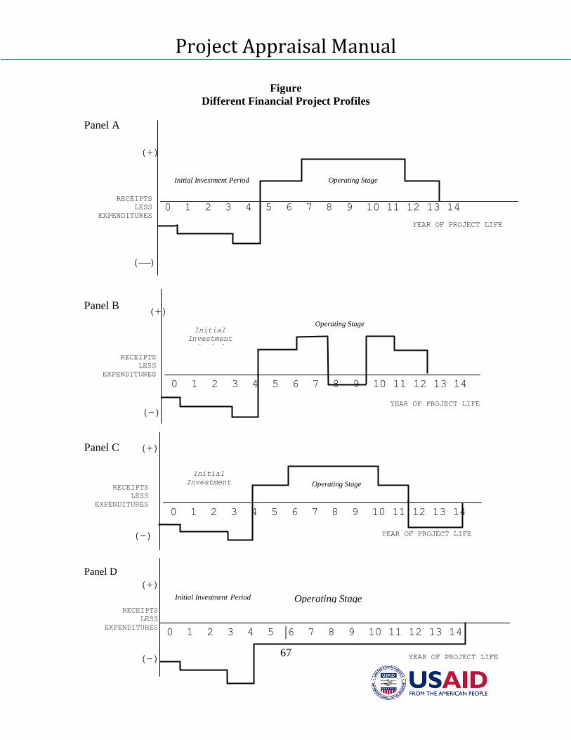
Project Appraisal Manual
67
Figure
Different Financial Project Profiles
Panel A
Panel B
Panel C
Panel D
Operating Stage
(+)
Initial Investment Period
0 1 2 3 4 5 6 7 8 9 10 11 12 13 14 RECEIPTS
LESS
EXPENDITURES
()
YEAR OF PROJECT LIFE
(+)
Operating Stage Initial
Investment
Period
0 1 2 3 4 5 6 7 8 9 10 11 12 13 14
RECEIPTS
LESS
EXPENDITURES
(-) YEAR OF PROJECT LIFE
Operating Stage
(+)
Initial
Investment
Period
0 1 2 3 4 5 6 7 8 9 10 11 12 13 14
RECEIPTS
LESS
EXPENDITURES
(-) YEAR OF PROJECT LIFE
(+)
Initial Investment Period
0 1 2 3 4 5 6 7 8 9 10 11 12 13 14
Operating Stage RECEIPTS
LESS
EXPENDITURES
(-) YEAR OF PROJECT LIFE
Project Appraisal Manual
68
Investment Plan
The first step in the construction of a
financial cash flow statement is the
formulation of an investment plan for the
project based on the information
developed in the technical, demand,
manpower, and financing modules. The
investment plan consists of two sections:
the first deals with the expenditure on
new acquisitions, and the opportunity
cost of existing assets, and the second
section deals with the financing aspects
of the proposed investment. If there are
different scales and/or locations under
consideration, corresponding investment
plans for each scale and/or location
should be formulated.
The table below provides an illustration
for sections an investment plan for a
water supply project. All data in the
investment plan regarding the
expenditures on new acquisitions, and
the opportunity cost of existing assets, if
applicable, are included in the cash flow
statement. Financing data is included in
some statements but not others
depending on the point of view as
explained below11
.
Data and Data Breakdown
11
The sales revenues and cash expenditures in a
project will occur almost on a continuous basis.
However, these inflows and outflows have to be
lumped together for each time period that may be
a year, a quarter or a month. In this manual, as a
matter of convention, all inflows and out flows
are supposed to occur at the end of the
corresponding time period. One could very well
assume that they all occur at the beginning of the
time period. The important thing is to adopt any
one of these conventions and then be consistent.
Once time schedules and deadlines are
formulated, expenditures should be
broken down by year of expected
expenditure. Expenditures on
internationally traded items should be
separated from expenditures on items
that are not traded internationally. This
breakdown is important for analyzing
foreign exchange implications and later
for estimating the economic costs
associated with these expenditures.
Each expenditure item should be broken
down into its components, whenever
possible and appropriate. For example,
the final cost of an installed plant should
be broken down by what suppliers
receive, import tariffs, value added
taxes, and/or any other payment to the
government, freight charges, handling
charges, installation costs, etc.
Investment credits or other forms of
subsidies should be explicitly presented.
Civil works and building construction
should be broken down into raw
material, and the different types of labor.
These breakdowns are necessary for
conducting the economic analysis of the
project and are also important for
providing a clear understanding of its
cost structure. Moreover identifying the
recipients of the various payments
enables the project analysts and
economists to determine some of the
beneficiaries of the project.
The first section of table below presents
the investment expenditures for the
water supply project in the manner
described above.
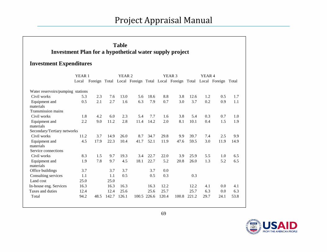
Project Appraisal Manual
69
Table
Investment Plan for a hypothetical water supply project
Investment Expenditures
YEAR 1 YEAR 2 YEAR 3 YEAR 4
Local Foreign Total Local Foreign Total Local Foreign Total Local Foreign Total
a. Water reservoirs/pumping stations
Civil works 5.3 2.3 7.6 13.0 5.6 18.6 8.8 3.8 12.6 1.2 0.5 1.7
Equipment and
materials
0.5 2.1 2.7 1.6 6.3 7.9 0.7 3.0 3.7 0.2 0.9 1.1
b. Transmission mains
Civil works 1.8 4.2 6.0 2.3 5.4 7.7 1.6 3.8 5.4 0.3 0.7 1.0
Equipment and
materials
2.2 9.0 11.2 2.8 11.4 14.2 2.0 8.1 10.1 0.4 1.5 1.9
c. Secondary/Tertiary networks
Civil works 11.2 3.7 14.9 26.0 8.7 34.7 29.8 9.9 39.7 7.4 2.5 9.9
Equipment and
materials
4.5 17.9 22.3 10.4 41.7 52.1 11.9 47.6 59.5 3.0 11.9 14.9
d. Service connections
Civil works 8.3 1.5 9.7 19.3 3.4 22.7 22.0 3.9 25.9 5.5 1.0 6.5
Equipment and
materials
1.9 7.8 9.7 4.5 18.1 22.7 5.2 20.8 26.0 1.3 5.2 6.5
e. Office buildings 3.7 3.7 3.7 3.7 0.0
g. Consulting services 1.1 1.1 0.5 0.5 0.3 0.3
h. Land cost 25.0 25.0
i. In-house eng. Services 16.3 16.3 16.3 16.3 12.2 12.2 4.1 0.0 4.1
j. Taxes and duties 12.4 12.4 25.6 25.6 25.7 25.7 6.3 0.0 6.3
Total 94.2 48.5 142.7 126.1 100.5 226.6 120.4 100.8 221.2 29.7 24.1 53.8
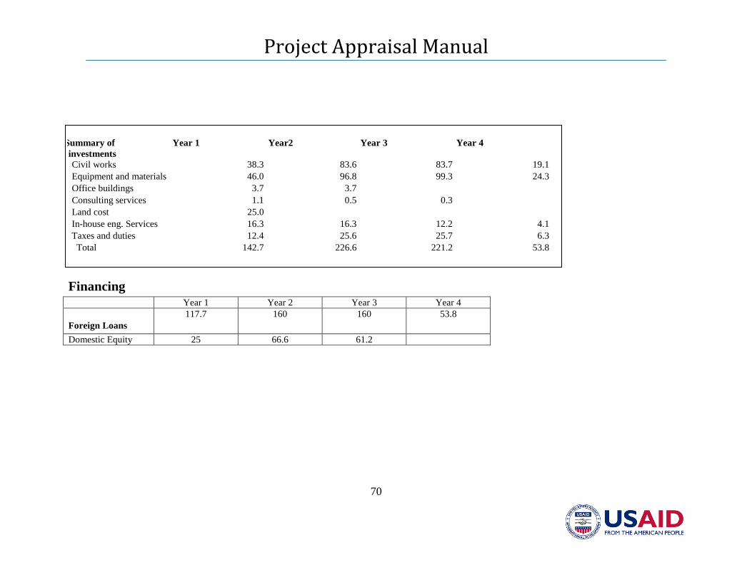
Project Appraisal Manual
70
Summary of
investments
Year 1 Year2 Year 3 Year 4
Civil works 38.3 83.6 83.7 19.1
Equipment and materials 46.0 96.8 99.3 24.3
Office buildings 3.7 3.7
Consulting services 1.1 0.5 0.3
Land cost 25.0
In-house eng. Services 16.3 16.3 12.2 4.1
Taxes and duties 12.4 25.6 25.7 6.3
Total 142.7 226.6 221.2 53.8
Financing
Year 1 Year 2 Year 3 Year 4
Foreign Loans
117.7 160 160 53.8
Domestic Equity 25 66.6 61.2
Project Appraisal Manual
71
Opportunity cost of existing assets
If the project under consideration is an
ongoing concern or a rehabilitation
project where some of the project’s old
assets are integrated into the proposed
facilities, the opportunity cost of these
assets should be included in the cash
flow statement together with the
expenditure on new acquisitions. See
box below for why it is necessary to
include the opportunity cost of an
existing asset in the cash flow statement.
It is necessary to distinguish the
“opportunity cost” of an asset from the
“sunk cost” of an asset. The opportunity
cost of using an asset in a specific
project is the benefit foregone by not
putting the asset to its best alternative
use. To measure the opportunity cost of
an asset, a monetary value has to be
assigned to it that should be equal to
what has been sacrificed by using it in
the project rather than in its next best
use. On the other hand, the value of an
asset is treated as a sunk cost if the asset
has no alternative use. The opportunity
cost of such an asset is zero.
For the sake of illustration, take an asset
that has been purchased by a firm and it
can be used to make only one product
and nothing else. Also, it cannot be
leased to any other firm and its scrap
value is negligible. In other words, the
asset has no alternative value except in
its current operations. Clearly its
opportunity cost is zero. Sunk cost
involves neither current nor future
opportunity cost and therefore should
have no influence in deciding what will
be the most profitable thing to do. It
should, however, be noted that while the
sunk cost of an asset should not be
counted as a cost to a new project in
examining its feasibility, any
outstanding liabilities due to that asset
may become the liability of the new
project if the ownership is the same.
Major items of the existing assets should
be broken down, similar to the
expenditure on new acquisition into
traded and non-traded and into a
reasonable number of components
whenever possible. The opportunity cost
of the existing assets is generally
included in the first year (conventionally
year 0) of the project’s cash flow profile.
This is because the assets could be sold
at that time if the project is not feasible.
The financial opportunity cost of an
existing asset is the highest financial
price that it could be sold for. The
financial price paid for the assets when
they were first acquired is irrelevant and
should never be used to reflect the
opportunity cost of an asset. The highest
financial price is typically the higher of
the in-use value of the asset and its
liquidation value. The in-use value of
the asset is what it would sell for if it
were to be used as an ongoing concern.
The liquidation value is what the asset
would sell for if broken into its different
components and sold in parts. For
example, when considering the
opportunity cost of any production plant,
one should consider the in-use value of
the plant if it continues to be operated as
is, and its financial value if dismantled
and the different parts are sold
separately.
The most accurate way to determine in-
use and liquidation values is through
reliable market assessors. When
estimating in-use values using assessors,
the assessor’s fees should be subtracted
from the quoted value to obtain the net
Project Appraisal Manual
72
in-use value. Also when assessors give a
liquidation value for a project’s assets,
the assessors’ fees as well as the
expenditures incurred in dismantling the
assets should be netted from the quoted
price to obtain a net liquidation value.
In the absence of an assessor, a rough
estimate of the plant’s value can be
obtained by using the rate of economic
depreciation of the assets. The
economic depreciation rate for an asset
reflects the loss in the market value of
the asset and is generally different from
the depreciation rate used for tax
purposes. Economic depreciation rates
for plants and equipment may be
obtained from the plant manufacturer;
technical journals may contain
information on depreciation patterns;
also insurance companies that insure a
plant’s assets have some estimates for
the plant’s rate of economic
depreciation.
Suppose the installed cost of a
wastewater treatment plant was A0 in
1995. Also suppose that the plant has an
economic life T, and that the plant’s
annual rate of economic depreciation is
de. If the price index has risen from I1995
to I2005, the in-use value of the plant can
be estimated as follows:
In-use value (2005) = A0×(1 – 10×de)×(I2005 / I1995)
In a case where the rate of economic
depreciation is the same as the rate of
straight line depreciation,
In-use value (2005) = A0×(1 – 10/T)×(I2005 / I1995)
The term in the first set of parentheses
represents the remaining proportion of
the value of the plant in purchasing
power of 1995, and the term in the
second set of parentheses adjusts the in-
use value of the asset from the 1995
price level to the 2005 price level.
Investment financing
The second half of the investment plan
deals with the means and schedules of
financing the investment expenditures.
This data should be largely prepared in
the financing plan already discussed.
The sources of finance used whether
equity or grants, domestic short term and
long term loans, foreign loans, suppliers’
credit, concessionary loans and other
forms of foreign aid should be identified
and the disbursement schedules should
be formulated. The second section of
the investment plan illustrated in the
table above presents an example of a
financing plan.
Whether the data in the financing section
of the investment plan is included in the
cash flow statement or not depends on
the point of view considered. When
appraising the project from an owner’s
point of view, the loan disbursement is
an inflow, and the repayment is an
outflow as the owner is looking to the
net receipts after paying any debtors or
other shareholders. The analysis of the
financial performance of the total
invested capital, however, is not
concerned with the financing but is
looking to determine the financial
viability of the project to all investors
irrespective of the sources and terms of
financing. Different points of view are
discussed below.
Operating Plan
The operating plan is developed on the
basis of the data formulated and
organized in the technical, demand
(market), and manpower modules. It
Project Appraisal Manual
73
includes all cash receipts generated from
the operations of the business and all
operating expenditures. Expenditures
and corresponding receipts should be
projected by year of operation. Similar
to investment expenditures, data
breakdowns are necessary in operating
plan as well. Operating expenditures
should be broken down into
internationally-traded and internationally
non-traded items; and each expenditure
item should be broken down into its
components, whenever possible. For
example, maintenance expenditures
should be broken down into materials
and labor. Expenditures on different
types of labor (skilled, unskilled, etc.)
should be identified and recorded
separately. Any taxes or subsidies
associated with the operating
expenditures should also be identified
and recorded separately whenever
possible. These breakdowns are
necessary for conducting the economic
analysis of the project and for providing
a better understanding of the cost
structure of the operating expenditures.
The following table presents an
illustration of an operating plan for a
hypothetical water supply project.
Direct data requirements for a cash flow
statement are slightly different from, and
may not be as readily available as data
requirements for income statements and
balance sheets.12
For example, an
income statement includes sales and
purchases, while a cash flow statement
includes receipts and expenditures.
Sales and purchases include credit as
12
One of the main reasons for more readily
available information for balance sheets and
income statements is that these statements are
often required by law for disclosure and tax
purposes.
well as cash transactions, while receipts
and expenditures are cash only. Even
though direct data requirements for cash
flow statements may not exist, a cash
flow statement can be constructed from
the information in a set of balance sheets
and income statements. A few important
distinctions between variables included
in a cash flow statement and variables in
other financial statements are discussed
below. The distinction generally stems
from the fact that non-cash impacts (with
the exception of opportunity costs) are
not included in the cash flow statement.
Adjustment of Sales
Needless to say, a project’s viability is
not only determined by the sales it
generates but also by the timing of the
cash receipts from the sales. A cash
flow statement records sales transactions
only when the cash from the transaction
is received. Typically projects forecast
their sales as a single line item which
comprises both credit and cash
transactions. Only cash sales are
included in a cash flow statement. Many
government projects and firms provide
their goods and services to their
customers without receiving immediate
cash payments. Reasons for this vary. In
some cases, it could be government
policy to provide such credits, which
indeed serve as short-term credit, to
assist certain project sponsors. In other
cases, a credit sale could be involuntary
where it takes the customers several
months to pay for the services they
consume, such as in the case of water
and electricity.
A distinction must be made between
sales and cash receipts. When a project
makes a sale, the good or service may be
delivered to the customer but no money
Project Appraisal Manual
74
transferred from the customer to the
project. At this point the project’s
accountants will record that the project
has an asset called Accounts Receivable
(AR) equal to the amount of the sale, or
the proportion of it that was not in cash.
In other words, the buyer owes the
project for the goods or services that he
has purchased and not yet paid for.
Until the buyer has paid for what he has
received, the transaction will have no
impact on the cash flow statement.
When the buyer pays for the items that
he previously bought from the project,
the project’s accountant records a
decrease in accounts receivable by the
amount that the buyer has paid and an
increase in cash receipts. Only then are
these cash receipts included in the cash
flow statement as inflows.
The cash receipts for any period equals
the sales during the period plus the
accounts receivable at the beginning of
the period less the accounts receivable at
the end of the period. The maximum
amount of cash a project can receive
during a period of time would be equal
to the new sales and the outstanding
receivables, if any. However if a
balance of accounts receivable that has
not been collected remains at the end of
the period, then this balance should be
netted from the maximum.
This is illustrated in the figure below.
The project makes 1000 Dinars worth of
sales during the first year, of which 600
Dinars are in cash and 400 Dinars are on
credit. The cash inflow for this year
should be 600 Dinars and not 1000
Dinars. Suppose the project’s sales are
2000 Dinars during the second year, and
at the end of the year, the outstanding
receivables owed to the project are 500
Dinars, then the cash receipts for this
year would be 1900 Dinars. These are
estimated as the beginning balance of
accounts receivables (400 Dinars) plus
the new sales during the year (2000
Dinars) less the final balance of accounts
receivable (500 Dinars). If all the
project’s sales for the year were cash and
all accounts receivable were collected,
then cash receipts for the year would
have been 2400 Dinars. However, given
that a remaining balance of 500 Dinars
in receivables, actual cash receipts are
only 1900 Dinars.
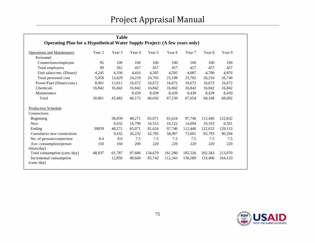
Project Appraisal Manual
75
Table
Operating Plan for a Hypothetical Water Supply Project: (A few years only)
Operations and Maintenance Year 2 Year 3 Year 4 Year 5 Year 6 Year 7 Year 8 Year 9
Personnel
Connections/employee 95 100 100 100 100 100 100 100
Total employees 99 262 457 457 457 457 457 457
Unit salary/mo. (Dinars) 4,245 4,330 4,416 4,505 4,595 4,687 4,780 4,876
Total personnel cost 5,058 13,629 24,219 24,703 25,198 25,702 26,216 26,740
Power/Fuel (Dinars/cum.) 8,961 13,011 16,672 16,672 16,672 16,672 16,672 16,672
Chemicals 16,842 16,842 16,842 16,842 16,842 16,842 16,842 16,842
Maintenance 8,439 8,439 8,439 8,439 8,439 8,439
Total 30,861 43,482 66,172 66,656 67,150 67,654 68,168 68,692
Production Schedule
Connections
Beginning 38,839 48,271 65,071 81,624 97,746 112,440 122,632
New 9,432 16,799 16,553 16,122 14,694 10,193 6,501
Ending 38839 48,271 65,071 81,624 97,746 112,440 122,632 129,133
Cumulative new connections 9,432 26,232 42,785 58,907 73,601 83,793 90,294
No. of persons/connection 8.4 8.0 7.5 7.5 7.5 7.5 7.5 7.5
Ave. consumption/person
(liters/day)
150 160 200 220 220 220 220 220
Total consumption (cum./day) 48,937 61,787 97,606 134,679 161,280 185,526 202,343 213,070
Incremental consumption
(cum./day)
12,850 48,669 85,742 112,343 136,589 153,406 164,133
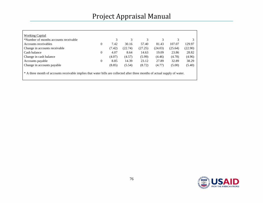
Project Appraisal Manual
76
Working Capital
*Number of months accounts receivable 3 3 3 3 3 3
Accounts receivables 0 7.42 30.16 57.40 81.43 107.07 129.97
Change in accounts receivable (7.42) (22.74) (27.25) (24.03) (25.64) (22.90)
Cash balance 0 4.07 8.64 14.63 19.09 23.86 28.82
Change in cash balance (4.07) (4.57) (5.99) (4.46) (4.78) (4.96)
Accounts payable 0 8.85 14.39 23.12 27.89 32.89 38.29
Change in accounts payable (8.85) (5.54) (8.72) (4.77) (5.00) (5.40)
* A three month of accounts receivable implies that water bills are collected after three months of actual supply of water.
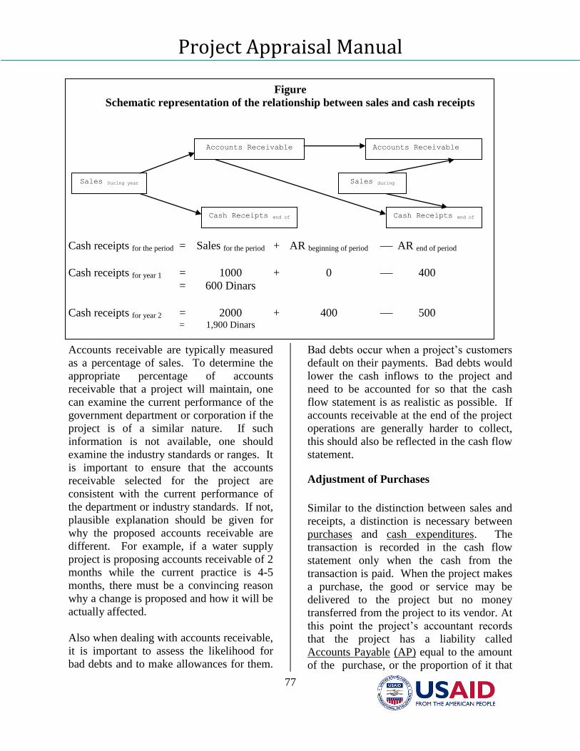
Project Appraisal Manual
77
Figure
Schematic representation of the relationship between sales and cash receipts
Cash receipts for the period = Sales for the period + AR beginning of period AR end of period
Cash receipts for year 1 = 1000 + 0 400
= 600 Dinars
Cash receipts for year 2 = 2000 + 400 500 = 1,900 Dinars
Accounts receivable are typically measured
as a percentage of sales. To determine the
appropriate percentage of accounts
receivable that a project will maintain, one
can examine the current performance of the
government department or corporation if the
project is of a similar nature. If such
information is not available, one should
examine the industry standards or ranges. It
is important to ensure that the accounts
receivable selected for the project are
consistent with the current performance of
the department or industry standards. If not,
plausible explanation should be given for
why the proposed accounts receivable are
different. For example, if a water supply
project is proposing accounts receivable of 2
months while the current practice is 4-5
months, there must be a convincing reason
why a change is proposed and how it will be
actually affected.
Also when dealing with accounts receivable,
it is important to assess the likelihood for
bad debts and to make allowances for them.
Bad debts occur when a project’s customers
default on their payments. Bad debts would
lower the cash inflows to the project and
need to be accounted for so that the cash
flow statement is as realistic as possible. If
accounts receivable at the end of the project
operations are generally harder to collect,
this should also be reflected in the cash flow
statement.
Adjustment of Purchases
Similar to the distinction between sales and
receipts, a distinction is necessary between
purchases and cash expenditures. The
transaction is recorded in the cash flow
statement only when the cash from the
transaction is paid. When the project makes
a purchase, the good or service may be
delivered to the project but no money
transferred from the project to its vendor. At
this point the project’s accountant records
that the project has a liability called
Accounts Payable (AP) equal to the amount
of the purchase, or the proportion of it that
Sales During year
1
Accounts Receivable end of year 1
Cash Receipts end of
year 1
Accounts Receivable end of year 2
Cash Receipts end of
year 2
Sales during
year 2
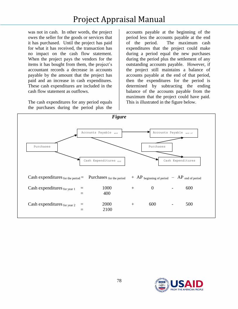
Project Appraisal Manual
78
was not in cash. In other words, the project
owes the seller for the goods or services that
it has purchased. Until the project has paid
for what it has received, the transaction has
no impact on the cash flow statement.
When the project pays the vendors for the
items it has bought from them, the project’s
accountant records a decrease in accounts
payable by the amount that the project has
paid and an increase in cash expenditures.
These cash expenditures are included in the
cash flow statement as outflows.
The cash expenditures for any period equals
the purchases during the period plus the
accounts payable at the beginning of the
period less the accounts payable at the end
of the period. The maximum cash
expenditures that the project could make
during a period equal the new purchases
during the period plus the settlement of any
outstanding accounts payable. However, if
the project still maintains a balance of
accounts payable at the end of that period,
then the expenditures for the period is
determined by subtracting the ending
balance of the accounts payable from the
maximum that the project could have paid.
This is illustrated in the figure below.
Figure
Cash expenditures for the period = Purchases for the period + AP beginning of period – AP end of period
Cash expenditures for year 1 = 1000 + 0 - 600
= 400
Cash expenditures for year 2 = 2000 + 600 - 500
= 2100
Purchases
During year 1
Accounts Payable end
of year 1
Cash Expenditures end
of year 1
Accounts Payable end of
year 2
Cash Expenditures
end of year 2
Purchases
during year 2
Project Appraisal Manual
79
Suppose the project purchases inputs for
1000 Dinars during the first year of the
project’s operations. Sixty percent of these
purchases are on a credit basis. Cash
expenditures relating to purchases for the
year are 400 Dinars and not 1000 Dinars.
Suppose that the project purchases
additional inputs worth 2000 Dinars during
the second year, and at the end of the year,
the remaining accounts payable to be paid
by the project are 500 Dinars, then the cash
expenditures for this year would be 2100
Dinars. These are estimated as the
beginning balance of accounts payable for
the year (600 Dinars) plus the new
purchases during the year (2000 Dinars) less
the final balance of accounts payable (500
Dinars). If all the project’s purchases during
the year were paid for in cash and all
outstanding accounts owed by the project
were paid, then cash expenditures for the
year would have been 2600 Dinars.
However, given that there is a remaining
balance of 500 Dinars in accounts payable,
actual cash expenditures are only 2100
Dinars
Accounts payable are typically measured as
a percentage of total purchases or that of a
major input. The appropriate amount of
accounts payable that a project will maintain
can be determined on the basis of the current
performance of the government department
if the project is of a similar nature. If such
information is not available, one should
examine the industry standards or ranges. It
is important to ensure that the accounts
payable on which the cash flows will be
based are consistent with the industry
norms.
Adjustment for Changes in Cash Balance
Increases and decreases in cash balances
owned by the project can take place even
when no change occurs in sales, accounts
receivable, purchases or accounts payable.
For example, when cash is set aside for the
transactions of the business, it is a use of
cash which is represented as an outflow in
the cash flow statement. Similarly a
decrease in cash held by the project is a
source of cash for the project and its
sponsors, and is a cash inflow. Note that
any cash set aside will ultimately all be
released back to the project as an inflow at
the end of the project.
The amount of cash to be held for
facilitating the transactions of the business is
typically a percentage of the project’s
expenditures, sales, or major purchases and
it can be determined by examining the
performance of similar projects in the same
sector or industry.
To illustrate how changes in the cash
balance are incorporated in the cash flow
statement, consider the following example.
Suppose that a project has the sales profile
given below and that the project’s cash
balance for any time period is 20% of the
project’s projected sales for that time period.
Note that the initial amount of cash balance
(20,000 Dinars) is treated as a cash outflow
because this amount has to be set aside.
Subsequent increases also represent
outflows. At the end of the project’s
operations when holding cash is no longer
necessary, the entire amount of cash held
(38,000 Dinars) is released back into the
project and is treated as an inflow.
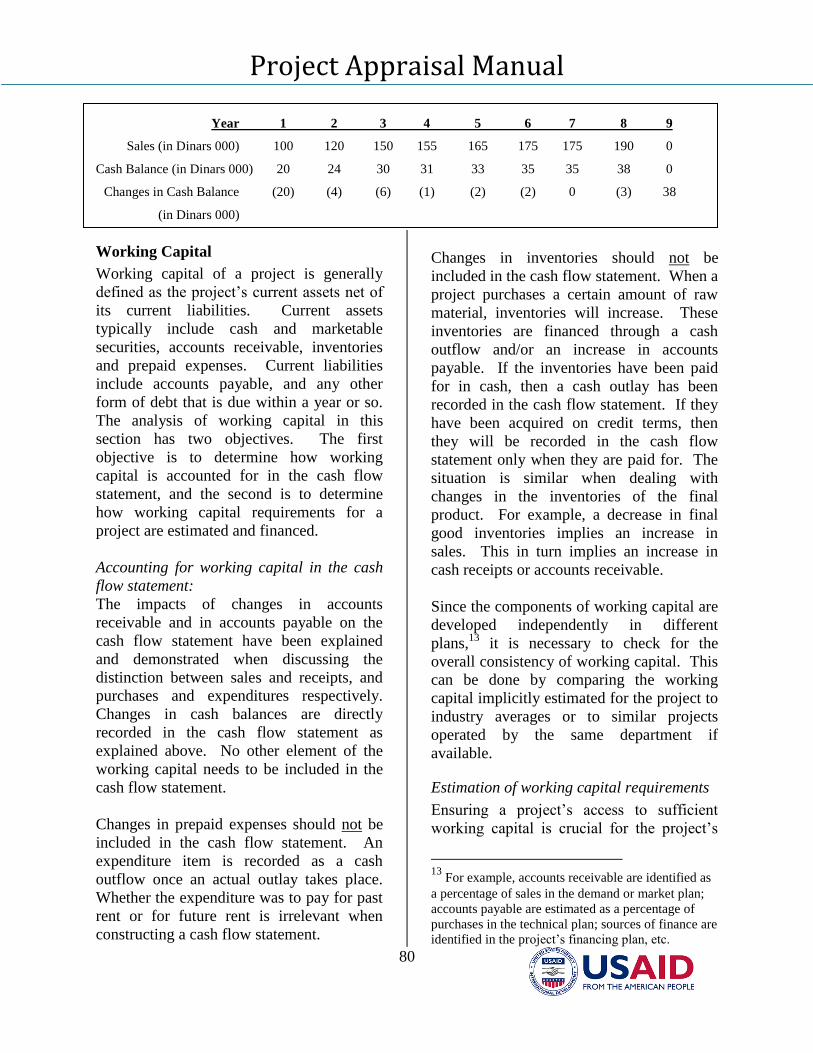
Project Appraisal Manual
80
Year 1 2 3 4 5 6 7 8 9
Sales (in Dinars 000) 100 120 150 155 165 175 175 190 0
Cash Balance (in Dinars 000) 20 24 30 31 33 35 35 38 0
Changes in Cash Balance (20) (4) (6) (1) (2) (2) 0 (3) 38
(in Dinars 000)
Working Capital
Working capital of a project is generally
defined as the project’s current assets net of
its current liabilities. Current assets
typically include cash and marketable
securities, accounts receivable, inventories
and prepaid expenses. Current liabilities
include accounts payable, and any other
form of debt that is due within a year or so.
The analysis of working capital in this
section has two objectives. The first
objective is to determine how working
capital is accounted for in the cash flow
statement, and the second is to determine
how working capital requirements for a
project are estimated and financed.
Accounting for working capital in the cash
flow statement:
The impacts of changes in accounts
receivable and in accounts payable on the
cash flow statement have been explained
and demonstrated when discussing the
distinction between sales and receipts, and
purchases and expenditures respectively.
Changes in cash balances are directly
recorded in the cash flow statement as
explained above. No other element of the
working capital needs to be included in the
cash flow statement.
Changes in prepaid expenses should not be
included in the cash flow statement. An
expenditure item is recorded as a cash
outflow once an actual outlay takes place.
Whether the expenditure was to pay for past
rent or for future rent is irrelevant when
constructing a cash flow statement.
Changes in inventories should not be
included in the cash flow statement. When a
project purchases a certain amount of raw
material, inventories will increase. These
inventories are financed through a cash
outflow and/or an increase in accounts
payable. If the inventories have been paid
for in cash, then a cash outlay has been
recorded in the cash flow statement. If they
have been acquired on credit terms, then
they will be recorded in the cash flow
statement only when they are paid for. The
situation is similar when dealing with
changes in the inventories of the final
product. For example, a decrease in final
good inventories implies an increase in
sales. This in turn implies an increase in
cash receipts or accounts receivable.
Since the components of working capital are
developed independently in different
plans,13
it is necessary to check for the
overall consistency of working capital. This
can be done by comparing the working
capital implicitly estimated for the project to
industry averages or to similar projects
operated by the same department if
available.
Estimation of working capital requirements
Ensuring a project’s access to sufficient
working capital is crucial for the project’s
13
For example, accounts receivable are identified as
a percentage of sales in the demand or market plan;
accounts payable are estimated as a percentage of
purchases in the technical plan; sources of finance are
identified in the project’s financing plan, etc.
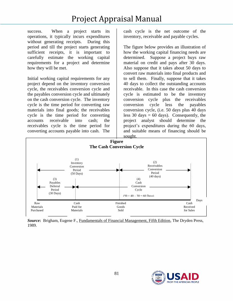
Project Appraisal Manual
81
success. When a project starts its
operations, it typically incurs expenditures
without generating receipts. During this
period and till the project starts generating
sufficient receipts, it is important to
carefully estimate the working capital
requirements for a project and determine
how they will be met.
Initial working capital requirements for any
project depend on the inventory conversion
cycle, the receivables conversion cycle and
the payables conversion cycle and ultimately
on the cash conversion cycle. The inventory
cycle is the time period for converting raw
materials into final goods; the receivables
cycle is the time period for converting
accounts receivable into cash; the
receivables cycle is the time period for
converting accounts payable into cash. The
cash cycle is the net outcome of the
inventory, receivable and payable cycles.
The figure below provides an illustration of
how the working capital financing needs are
determined. Suppose a project buys raw
material on credit and pays after 30 days.
Also suppose that it takes about 50 days to
convert raw materials into final products and
to sell them. Finally, suppose that it takes
40 days to collect the outstanding accounts
receivable. In this case the cash conversion
cycle is estimated to be the inventory
conversion cycle plus the receivables
conversion cycle less the payables
conversion cycle, (i.e. 50 days plus 40 days
less 30 days = 60 days). Consequently, the
project analyst should determine the
project’s expenditures during the 60 days,
and suitable means of financing should be
sought.
Figure
The Cash Conversion Cycle
Source: Brigham, Eugene F., Fundamentals of Financial Management, Fifth Edition, The Dryden Press,
1989.
(50 + 40 – 30 = 60 Days)
(4)
Cash
Conversion
Cycle
Cash
Receivedfor Sales
Finished
GoodsSold
Cash
Paid forMaterials
Raw
MaterialsPurchased
Days
(3)
Payables
Deferral
Period(30 Days)
(1)
Inventory
Conversion
Period(50 Days)
(2)
Receivables
Conversion
Period(40 days)
Project Appraisal Manual
82
The cash conversion cycle on which the
working capital requirements are based is
typically much shorter than the unit of time
used in the cash flow statement which is
generally one year. In other words, a net
cash flow for the first year of operations will
reflect the total receipts generated during the
year net of total expenditures without
shedding any light on whether there is
enough working capital to get the project
started and keep it in progress. It is quite
probable that the net cash flow for the first
year of operations is indeed positive but not
enough working capital has been secured to
ensure that the project continues to function
smoothly. Consequently, it is necessary that
working capital requirements for a project
are explicitly worked out, and the
appropriate means of financing identified.
Estimation of Income Tax Liability
Income taxes, if expected to be paid by the
project, should be included in the cash flow
statement. The income tax liability is
estimated on the basis of the project’s
income statement and follows the
accounting and tax rules of the country/state.
Year by year estimates of cost of goods sold,
interest expense, depreciation expense,
overheads (if not included in costs of goods
sold) are subtracted from the project’s
revenues to estimate the project’s earning
before taxes. When estimating the income
tax liability, provisions for loss carry
forward should be taken into account.
Cessation of Project Operations
When a new project acquires an asset, the
entire expenditure on the asset is accounted
for in the cash flow statement at the time
that the expenditure actually occurs. It is
quite possible, however, that the life of the
project does not coincide with the life of all
its assets, or that the span of the analysis
does not extend as far in the future as the
project may be expected to operate; for
example, railway projects or irrigation
systems. If either of the two conditions
exists, then the residual value of the asset,
i.e. the value of the part of the asset that has
not been used should be included in the cash
flow statement as an inflow in the year
following the cessation of operations.
Consider the following example to illustrate
the point. Suppose a project acquires a
piece of machinery for one million Dinars in
1998. The machinery has an economic life
of 10 years and the expected life of the
project is 7 years. The expected market
value of the machine at the end of the
seventh year is 150,000 Dinars. If we were
only to include the expenditure on the
machinery (one million Dinars) as an
outflow without including the residual value
(150,000 Dinars) as an inflow, then we
would be penalizing the project.
As a matter of convention, residual values
are recorded in the cash flow statement in
the year following the cessation of
operations. The underlying assumption is
that liquidating assets may require a few
months. When determining the residual
value of the assets at the end of the project,
it is preferable to break down all the assets
into different categories: land, building,
equipment, vehicles, etc. The residual value
is taken as the higher of the in-use or
liquidation value. The in-use value of the
plant is the value of the plant under the
assumption that it will continue to operate as
an on-going concern. The liquidation value
is the value of the assets if all components of
the project are sold separately and perhaps
even the plant is taken apart and liquidated.
This approach is similar to that taken when
estimating the opportunity cost of existing
assets. It is, however, more difficult in this
case to estimate the in-use and liquidation
values since we are dealing with a situation
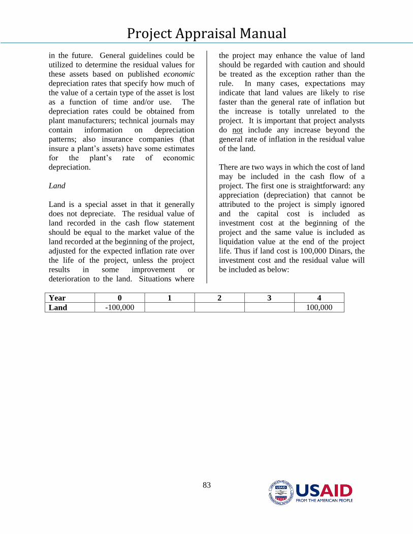
Project Appraisal Manual
83
in the future. General guidelines could be
utilized to determine the residual values for
these assets based on published economic
depreciation rates that specify how much of
the value of a certain type of the asset is lost
as a function of time and/or use. The
depreciation rates could be obtained from
plant manufacturers; technical journals may
contain information on depreciation
patterns; also insurance companies (that
insure a plant’s assets) have some estimates
for the plant’s rate of economic
depreciation.
Land
Land is a special asset in that it generally
does not depreciate. The residual value of
land recorded in the cash flow statement
should be equal to the market value of the
land recorded at the beginning of the project,
adjusted for the expected inflation rate over
the life of the project, unless the project
results in some improvement or
deterioration to the land. Situations where
the project may enhance the value of land
should be regarded with caution and should
be treated as the exception rather than the
rule. In many cases, expectations may
indicate that land values are likely to rise
faster than the general rate of inflation but
the increase is totally unrelated to the
project. It is important that project analysts
do not include any increase beyond the
general rate of inflation in the residual value
of the land.
There are two ways in which the cost of land
may be included in the cash flow of a
project. The first one is straightforward: any
appreciation (depreciation) that cannot be
attributed to the project is simply ignored
and the capital cost is included as
investment cost at the beginning of the
project and the same value is included as
liquidation value at the end of the project
life. Thus if land cost is 100,000 Dinars, the
investment cost and the residual value will
be included as below:
Year 0 1 2 3 4
Land -100,000 100,000
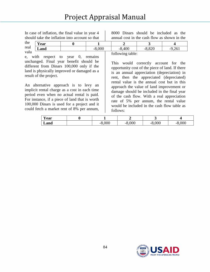
Project Appraisal Manual
84
In case of inflation, the final value in year 4
should take the inflation into account so that
the
real
valu
e, with respect to year 0, remains
unchanged. Final year benefit should be
different from Dinars 100,000 only if the
land is physically improved or damaged as a
result of the project.
An alternative approach is to levy an
implicit rental charge as a cost in each time
period even when no actual rental is paid.
For instance, if a piece of land that is worth
100,000 Dinars is used for a project and it
could fetch a market rent of 8% per annum,
8000 Dinars should be included as the
annual cost in the cash flow as shown in the
following table:
This would correctly account for the
opportunity cost of the piece of land. If there
is an annual appreciation (depreciation) in
rent, then the appreciated (depreciated)
rental value is the annual cost but in this
approach the value of land improvement or
damage should be included in the final year
of the cash flow. With a real appreciation
rate of 5% per annum, the rental value
would be included in the cash flow table as
follows:
Year 0 1 2 3 4
Land -8,000 -8,400 -8,820 -9,261
Year 0 1 2 3 4
Land -8,000 -8,000 -8,000 -8,000
Project Appraisal Manual
85
The financial analysis from different
points of view
For most projects that are directly
undertaken by the government, or involve
some government intervention in the form of
grants, loans or subsidies, there are several
stakeholders that would like to determine the
impact of the project on them. Stakeholders
are defined broadly to include all those
affected by the project. For example, the
stakeholders of a project may include the
owners, participating banks, any other
government department providing loans or
grants or collecting taxes, competitors,
workers, etc. It is therefore necessary to
conduct the analyses from the points of view
of the different important stakeholders to
ensure the project’s sustainability and
success. Even one powerful stakeholder
who is adversely affected by the project may
be able to derail the entire project.
The preceding sections outline the variables
that are generally included in the cash flow
statement while discussing how they are
presented. Some variables will be relevant
to the analysis from the point of view of one
stakeholder and not from that of another.
The most commonly-undertaken financial
analyses for government and government-
related projects are from the following
viewpoints:
i) Point of view of owner,
ii) Point of view of all investors
combined (banker’s point of view or total
investment point of view);
iii) Point of view of the Budget.
These points of view are discussed below
focusing on the differences in the variables
included in the analyses from the different
perspectives.
i) The Owner’s Point of View
The owner or sponsor of a project could be a
private investor (who may be receiving
some form of support from the government
or investing under some form of partnership
arrangement with the government) or a
government department or authority
undertaking a project. The appraisal of the
project from the owner’s perspective
includes all receipts and expenditures related
to the project in the cash flow statement to
determine whether he is made better off or
not. Consequently, the owner or sponsor of
the project receives the net cash flow after
paying off all other involved parties,
including the debt holders. The cash flow
statement from an owner’s point of view
includes the disbursement of the loan as an
inflow and all subsequent repayments of
loan and interest as expenditures. If the
project receives any grants or subsidies,
these should be included as receipts in the
cash flow statement; and if the project pays
taxes, these should be included as a cash
outflow. If the project sponsor is going to
give up an existing source of income to
undertake a project, the forgone earnings i.e.
the opportunity cost should be included as
an expenditure item in the cash flow
statement.
ii) The Total Investment (Banker’s) Point
of View
This point of view examines the returns to
the total invested capital. In other words,
this analysis disregards any distinctions in
the sources of finance. It asks whether the
financial receipts generated from the
operations of this project are sufficient to
cover the investment and operations
expenditures, and provide a sufficient return
or not. This point of view is also known as
the banker’s point of view because a bank
will be interested in examining the expected
receipts and expenditures to determine if the
Project Appraisal Manual
86
net cash flows from the total investment are
sufficient to cover the loan and interest
repayments. The banker typically has first
claim to the project’s assets and net cash
flows, and so the banker’s net cash flow is
the project’s gross receipts net of operating
and investment expenditures.14
The net
cash-flows from the total investment (also
called the “free cash flows”) are therefore
important in studying whether these cash
flows adequately cover the expected debt
repayment schedule. The size, pattern and
stability of these cash flows will affect the
patterns of debt repayment a project can
sustain. For example, if large net cash
flows are only expected late in the life of a
project, then the debt repayment has to be
structured to match that cash-flow pattern.
The only difference between the analysis
from the owner’s point of view and that
from the banker’s point of view is financing.
Specifically, the cash flow statement from
the total investment point of view includes
all items included from the owner’s
perspective except loan and loan
repayments.
iii) Budgetary Point of View
The purpose of the analysis from the
budgetary point of view is to ensure that the
relevant department has enough resources to
finance its obligations to the project during
both the investment and operational phases.
14
In few cases a subtle difference may exist between
the point of view of total invested capital and the
banker’s point of view. Consider, for example, a
government department that is encouraging the
construction of low-income housing projects by
repaying the interest on the housing loan. An analysis
from the total invested capital point of view will not be
concerned with the loan at all whether subsidized or
not. A banker however, will be definitely more in favor
of loaning to a project that receives a government loan
subsidy than a similar project that does not receive the
subsidy.
If the government department is the project
owner, then the only distinction between the
cash flow statement from the owner’s point
of view and from the budget point of view is
that opportunity costs are not taken into
account in the latter statement. If, on the
other hand, the government’s involvement is
in the form of providing some cheap credit,
subsidies, or grants, then the cash flow
statement only reflects these transactions.
Other perspectives
Although the three views outlined above are
the most typical points of view considered
when conducting the financial analysis, it is
important to analyze the impacts of the
project on all involved parties. For example,
if the project under consideration is likely to
have a negative impact on competitors, one
should anticipate their resistance and seek
feasible solutions. It is thus necessary to
estimate the magnitude of the damage to any
affected group. Affected groups could
include, competitors, suppliers of inputs,
downstream processors, etc.
Can This Analysis be Applied to Social
Sector Projects?
There are two aspects to this issue. First, is
financial analysis relevant for a social sector
project? One might argue that it is only the
economic analysis that is relevant and if a
social sector project is economically sound,
its financial analysis is of little consequence.
This view is, unfortunately, erroneous. The
financial cash flows are crucial for
projecting the cash position of the project in
the future and determining if and when cash
injections from external sources, including
the government budget, would be necessary.
This may make all the difference between a
successful project and a failed project. If the
project cannot be implemented due to
paucity of funds and lack of advance
planning, there is not going to be any
Project Appraisal Manual
87
economic benefits from the project. Also, it
is essential to have an accurate and detailed
financial analysis along with an economic
analysis in order to conduct the
distributional analysis of the project.
Another aspect of this issue is whether it is
possible to prepare a detailed financial cash
flow, as outlined in the preceding sections,
in case of a social sector project. The answer
is clearly yes. There is hardly any difference
between a social sector project and an
industrial project in preparing the cash flow
on the cost side. On the benefit side, one has
to include whatever revenues are being
generated by the project along with other
elements like grant/subsidy and liquidation
values. In the extreme case when the
services are being provided free of cost, the
revenues are zero and the financial analysis
is able to indicate the yearly requirement of
funds for continuing with the project. In
case, it is not necessary or possible to
quantify financial benefits in monetary
terms or when choosing among different
technologies for providing the same
services, one has to apply the “cost
effectiveness” criterion. For doing so, the
present values of alternative sets of costs
have to be estimated. This is only possible
when an elaborate and accurate cash flow
has been prepared. It is, therefore, evident
that the financial analysis as outlined above
is both essential and feasible in case of a
social project as well.
Finally, it is important to realize that an
analysis that includes the costs and benefits
to all involved parties constitutes the first
step in the economic analysis of the project.
Indeed, this is the starting point for the
discussions on the economic analysis
presented earlier. A summary of how
different financial items should be included
in the cash flow statement from different
points of view is given in the table below.
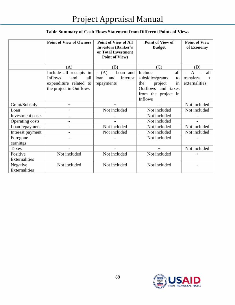
Project Appraisal Manual
88
Table Summary of Cash Flows Statement from Different Points of Views
Point of View of Owners
Point of View of All
Investors (Banker’s
or Total Investment
Point of View)
Point of View of
Budget
Point of View
of Economy
(A) (B) (C) (D)
Include all receipts in
Inflows and all
expenditure related to
the project in Outflows
= (A) – Loan and
loan and interest
repayments
Include all
subsidies/grants to
the project in
Outflows and taxes
from the project in
Inflows
= A – all
transfers +
externalities
Grant/Subsidy + + - Not included
Loan + Not included Not included Not included
Investment costs - - Not included -
Operating costs - - Not included -
Loan repayment - Not included Not included Not included
Interest payment - Not Included Not included Not included
Foregone
earnings
- - Not included -
Taxes - - + Not included
Positive
Externalities
Not included Not included Not included +
Negative
Externalities
Not included Not included Not included -
Project Appraisal Manual
89
The use of consistent prices in financial
appraisal: inflation treatment
When conducting a financial appraisal of a
project, it is necessary to develop price and
cost projections over the life of the project.
These prices are influenced by the forces of
demand and supply, which affect relative
prices, and by macroeconomic conditions,
which determine the general price level or
the level of inflation. Accurate forecasts of
the future growth in relative prices and in
the general price level are beyond the
responsibility of the project analyst.
However historical trends in growth of
prices coupled with recent and expected
government policies provide a good basis
for making these projections. Variations in
these assumptions should be tested using
sensitivity and risk analyses to determine
whether the project is robust enough to
withstand deviations from the assumptions
in the base case.
To understand the impact of inflation on the
financial viability of a project and how it is
incorporated in the analysis, it is necessary
to understand the distinction between the
different prices and price levels. These are
presented in sufficient detail in Annex at the
end of this chapter. Two prices however are
discussed below due to the important role
they can play in the financial analysis of
projects. These are the interest rate and the
price of foreign exchange.
Interest rate
The most important feature for integrating
expectations about the future rate of
inflation or expected growth in prices gPe
into the project evaluation is to ensure that
such expectations are consistent with the
projections of the nominal rate of interest (i).
Lenders increase the nominal interest rate on
the loans they give to compensate for the
anticipated loss in the real value of the loan
caused by inflation. As the inflation rate
increases, the nominal interest rate increases
to ensure that the present value of the
interest and principal payments does not fall
below the initial value of the loan.
The nominal interest rate i as determined by
the financial markets is made up of three
major components: a) the real interest rate r
which reflects the real time value of money
that lenders require in order to be willing to
forego consumption or other investment
opportunities, b) a risk factor R which
measures the compensation lenders demand
to cover the possibility of the borrower
defaulting on the loan, and c) a factor
(1+r+R)gPe which represents the
compensation for the expected loss in
purchasing power attributable to inflation.
Inflation reduces the future value of both the
loan repayments and real interest rate
payments. The expected rate of inflation for
each period of the loan is expressed as gPe.
Combining these factors, the nominal
(market) rate of interest i can be expressed
as:
i = r + R + (l + r + R) gPe
To explain this concept more fully, let us
consider the following financial scenarios.
When both risk and inflation are zero, a
lender would want to recover at least the real
time value of money. If the real interest rate
r is 5 percent, then the lender would charge
at least a 5 percent nominal interest rate. If
the lender anticipates that the future rate of
inflation gPe will be 10 percent, then she
would want to increase the nominal interest
rate charged to the borrower in order to
compensate for the loss in purchasing power
of the future loan and interest rate payments.
Maintaining the assumption that there is no
Project Appraisal Manual
90
gpde
i
risk to this loan, we can apply the above
equation to determine what nominal interest
rate she would need to charge to remain as
well off as when the inflation rate was zero.
i = r + R + (l + r + R) gPe
= (0.05) + (0) + (1+ 0.05 + 0)0.1
= 0.155 or 15.55%
Thus, the lender will need to charge a
nominal interest rate of at least 15.55
percent to achieve the same level of return
as in the scenario with zero inflation.
Generally, the real rate of interest is a fairly
constant value because it is primarily
determined by the productivity of
investment and the desire to consume and
save in the economy. Also, the value of the
risk premium for the various sectors and
investors is typically known. Given the real
interest rate, the risk premium and the
nominal interest rate, the expected rate of
inflation, which is implicit in the nominal
interest rate can be estimated by rearranging
the above equation as follows:
gPe = (i - r - R)/(1 + r + R)
If the rate of inflation is expected to change
through time and refinancing of the project's
debt is required, then the nominal interest
rate paid must be adjusted to be consistent
with this new expected rate of inflation.
This should have little or no direct effect on
the overall economic viability of the project
as measured by its NPV; however, it may
impose very severe constraints on the
liquidity position of the project because of
its impact on interest and principal payments
if not properly planned for.
Expected (nominal) exchange rate
A key financial variable in any project using
or producing tradable goods is the market
rate of exchange (EM
) between the Dinar
and the relevant foreign currency. This
market exchange rate is expressed as the
number of units of Dinars required to
purchase one unit of foreign exchange (F).
The market exchange rate is the current
(nominal) price of foreign exchange. The
market exchange rate needs to be projected
over the life of the project. The market rate
between the Dinar and the relevant foreign
currency can be expressed at any point in
time (t) as:
EM
t= (Dinars/F)t
The difference between the real price and
the nominal price of a good at a given point
in time, tn, lies in the cumulative inflation
measured from an arbitrary fixed point in
time, tb (base year), to the current point in
time, tn. If we choose the arbitrary point in
time to be the same as the current point in
time, then there is no difference between the
real and nominal prices. For convenience
when conducting the financial appraisal of a
project, we can select the first year of the
project, t0, as the arbitrary reference point or
base year. Consequently, the market
exchange rate and the real exchange rate
will be equal for that year, t0.
The cumulative inflation for Iraq over a
period of time is given by the domestic price
index ID. If we continue to use the reference
year, t0, as the base year, the domestic price
index at any point in time tn, can be
expressed as the cumulative change in the
price level from time t0, to tn This is given
as follows:
Where gi
pde is the rate
of inflation in the domestic economy.
)1(1 0
ni
i
pde
i
D
gI ttn
Project Appraisal Manual
91
Similarly the foreign price index at any
point in time tn, using the same reference
year, t0 as the base year, can be expressed as
the cumulative change in the price level
from time t0, to tn This is given as follows:
where gipfe
is the rate of inflation in the
foreign economy. Thus the market exchange
rate at time tn may be expressed in terms of
the real exchange rate and price indices as
follows:
I
I
I
I
I
I
D
t
F
tM
t
R
D
T
F
t
F
t
D
TR
n
n
n
n
n
n
EorE
F
Dinars
F
Dinars
RateEalExchange
Re
From this we conclude
The real exchange rate moves through time
by the forces of the country's demand and
supply for foreign exchange. From the point
of view of the project analyst, it is very
difficult to predict the movement of the real
exchange rate unless it is being artificially
maintained at a given level through tariffs or
quantitative restrictions on either the supply
or demand of foreign exchange. If the rate
is not artificially maintained, the analyst can
take the real exchange rate as constant
throughout the life of the project
The ratio of the two price indices is known
as the relative price index. If through time
the domestic economy faces a rate of
inflation different from that of a foreign
trading partner, the relative price index will
move over time. If the real exchange rate,
ER, is to remain constant in the presence of
inflation, then the change in the relative
price index must result in an equal change in
the market exchange rate.
Since the future real exchange rate is only
likely to be known with some uncertainty,
and the market exchange rate might not
adjust instantaneously to changes in the rate
of inflation, it is more realistic to allow
some flexibility in the estimation of the
market exchange rate. This is carried out by
assuming a range for the distribution of
possible exchange rates around an expected
mean real exchange rate. To incorporate
this aspect we write the above equation as
follows:
where K is a random variable with a mean
of 0.
Incorporating inflation in the financial
analysis
Much of the published literature on project
evaluation recommends the exclusion of
inflation from the appraisal process.15
At
best, these methods only account for
projected changes in relative prices of inputs
15
L. Squire and H.G. van der Tak, Economic Analysis of
Projects, (Baltimore: The Johns Hopkins University Press, 1975),
p. 38.
)1(1 0
ni
i
pfe
i
F
gI tt n
)
)1(
)1(
(*
)(*
1
1
0
0
ni
i
pfe
i
ni
i
pde
iRM
F
D
RM
g
gEE
II
EE
t
t
t
or
t
tt
n
n
n
n
)
)1(
)1(
)(1(*
1
1
0
0
ni
i
pfe
i
ni
i
pde
iRM
g
gEE
t
tk
t n
Project Appraisal Manual
92
and outputs over the life of the investment.16
However, experience with projects suffering
from financial liquidity and solvency
problems has demonstrated that inflation can
be a critical factor in the success or failure
of projects. Correctly designing a project to
accommodate both changes in relative prices
and changes in the rate of inflation may be
crucial for its ultimate survival.
Improper accounting for the impacts of
inflation when conducting the financial
analysis could have detrimental effects not
only on the financial sustainability of a
project but also on its economic viability.
Assumptions regarding inflation will have a
direct impact on the financial analysis of the
project and may require adjustments in the
operating or investment policies. Since an
inadequate treatment of inflation may
adversely affect the financial sustainability
of the project, ultimately the economic
viability of the project may be compromised
if inflation is not accounted for properly and
the necessary adjustments are not made. The
impacts of inflation on the financial analysis
of a project are discussed in the annexure.
16
All of the following authors recommend that expectations of
inflation of the general price level be ignored in the evaluation of
projects:
I.M.D. Little, and J.A. Mirrllees, Project Appraisal and Planning
for Development Countries (New York –basic books,
1974)
P. Dasgupta, A. Sen, and S. Marglin, Guidelines for Project
Evaluation, (Vienna: UNIDO, 1972).
Arnold C. Harberger, Project Evaluation Collected Papers,
(Chicago: Markham, 1973), p. 44.
A more satisfactory treatment of this issue is provided by M.
Roemer and Joseph J. Stern, The Appraisal of Development
Projects, A Practical Guide to Project Analysis with Case Studies
and Solutions, (New York: Praeger Publishers, 1975), pp. 73-74.
The authors present a rather mixed treatment of this issue in their
case 3 which is not entirely consistent; see also pp. 173-174.
It is important to realize that the ultimate
analysis of the financial cash flows should
always be carried out on a statement
prepared in real (i.e. net of inflation) Iraqi
Dinars. It is not easy to analyze nominal
(current) prices or nominal net cash flows as
one will be attempting to understand figures
that reflect two changes: changes in the real
price and changes in the general price level.
The correct treatment of inflation requires
that preparatory tables be made using
nominal prices, and at the very end cash
flow statements prepared in nominal prices
are deflated to obtain the cash flow
statements in real prices.
Outlined below is a method for
incorporating inflation into the financial
evaluation of a project in a consistent
manner. It draws mainly upon the
methodology in the Manual on Cost-Benefit
Analysis by Jenkins and Harberger.
When preparing the cash flow statement,
certain variables such as tax liabilities, cash
requirements, interest, and debt repayments
need to be estimated in the current prices of
the years they are to be incurred in. Other
variables making up the cash flow statement
are also presented in current prices and
initially cash flows in current prices are
developed. These cash flows are later
deflated and presented in real prices. By
constructing the financial analysis in this
manner, we ensure that first, all the effects
of inflation are consistently reflected in the
projected variables and second, all variables
are deflated by the projected increase in the
general level of prices.
The steps required to carry out the analysis
are as follows:
1. Estimate the future changes in the relative
prices for each input and output variable.
Project Appraisal Manual
93
This involves the examination of the present
and future demand and supply forces that
are expected to prevail in the market for the
item. For example, an examination of real
prices of many minerals will indicate that
they have been dropping a few percentage
points a year over the past decade. Real
wages, on the other hand tend to increase
over time as the economy grows.
2. Estimate or develop a set of assumptions
concerning the expected annual changes in
inflation over the life of the project.
3. Determine what the nominal rate of interest
will likely be over the lifetime of the project
given the expected changes in the price level
estimated above.
4. Combine the expected change in relative
prices with the expected change in the rate
of inflation to give the expected change in
the nominal price of an item.
5. Multiply the nominal prices for each item by
the projections of quantities of inputs and
outputs through time to express these
variables in the current year's prices of the
period in which they are expected to occur.
6. Begin the construction of a cash flow
statement using the current (nominal) values
for the inputs and outputs.
7. Construct a profit and loss statement for
each year of the project's life to determine
income tax liabilities with all variables
expressed in their nominal values.
Depreciation expenses, cost of goods sold,
and interest expenses and income tax
liabilities are estimated according to the
taxation laws of the country. The estimated
income tax liabilities are included in the
cash flow statement.
8. Estimate cash requirements and any changes
in the stock of cash that are reflected in the
cash flow statement.
9. Determine financing requirements along
with the interest payments and principal
repayments and include these items in the
cash flow statement. This completes the
construction of the projected variables in
terms of their current values inclusive of
inflation. Now we have a cash flow
statement in current prices from the owner’s
point of view.
10. Deflate all items in the owner’s cash flow
statement by the inflation price index to
arrive at real values for the cash flow
statement. Note that loans, interest
payments, and loan payments are included at
their deflated values in the determination of
the cash flow in real prices.
11. Discount the net financial cash flow to the
owners of the enterprise by either the real
(net of inflation) private opportunity cost of
equity financing if it is a private owner or by
the target financial rate of return (net of
inflation) set by the government if it is a
public sector enterprise.
12. Estimate the net financial cash flow from the
point of view of the total invested capital. In
this case, loans, interest and principal
payments do not enter into the calculation of
the net financial cash flow.
13. Calculate the net financial cash flow from
other points of view if necessary (budget,
etc.)
The case studies developed in this manual
provides illustrations of the inflation
treatment outlined above. The development
of pro-forma financial cash flow statements
in this way ensures that the impact of
inflation on the financial performance of the
project is correctly accounted for. At the
same time, the final financial analysis is
completed with the variables expressed in
terms of a constant general price level. In
this way, the movement of such variables as
receipts, labor costs and material costs can
be compared over time without being
distorted by changes in the general price
level.
When the financial analysis is carried
out in terms of real prices, it is essential
that the private opportunity costs of
capital or the target financial rates of
Project Appraisal Manual
94
return used as discount rates be
expressed net of any compensation for
the expected rate of inflation. In other
words, these discount rates must be real
and not nominal variables. If a nominal
interest rate or target rate of return is
used, the result will be a double
correction for the expected changes in
the general price level. Such practices
will greatly distort the conclusions of the
analysis concerning the financial
viability of the project.
It should be noted that the real financial
prices for the input and output variables
developed above are used as the basis on
which to estimate the economic values
for the benefits and costs of the project.
Once these economic costs and benefits
are estimated, an economic resource
flow statement is constructed. The
structure of the statement should be
similar to that of the financial cash flow
statement. Finally, the difference
between the two statements is analyzed
to determine the distributional impacts
of the project.
Project Appraisal Manual
95
Chapter VII: Financial Cost of Capital
Project Appraisal Manual
96
CHAPTER VII: FINANCIAL COST OF CAPITAL
In this section, we discuss the meaning,
interpretation and use of the financial cost of
capital in the context of valuing cash flow
profiles in project appraisal. Since the
financial cost of capital has a major impact
on the overall assessment of the investment
project from the financial point of view, it is
important to have a clear understanding of
the concept. Even though the assessment of
the project from the economic point of view
is the correct criterion for project selection,
the financial assessment could determine the
long term financial viability and
sustainability of the project. In addition, the
calculation of the financial cost of capital is
complicated by the existence of taxes and
debt financing.
Later, we explain how to adjust the financial
cost of capital in the presence of taxes and
debt financing. Moreover, as discussed
below, there are two different points of view
in the financial analysis, and for each point
of view, there is a corresponding cost of
capital.
As mentioned earlier in the previous
sections, cash flows that occur at different
points in time cannot be aggregated
together. A financial cash flow of for
example 1000 Iraqi Dinars that occurs in
one year from now has less value than a
cash flow of 1000 Iraqi Dinars that we can
receive immediately (right now). Through
the process of discounting, with the
appropriate discount rate(s), we “discount”
all the future values to the present time, and
sum them up to obtain the present value.
The concept of discounting also applies to
economic cash flows. To be consistent, we
have to discount the (nominal) financial cash
flows with the appropriate (nominal)
financial discount rate, and the
corresponding economic cash flows with the
appropriate economic discount rate, or more
formally, the economic opportunity cost of
capital (EOCK).
Nominal cash flow statement
To take account of the direct and indirect
impacts of inflation through various line
items in the cash flow statement, we
construct the cash flow statement in nominal
terms. As shown in the appendix, it is
incorrect to construct the cash flow
statement in real terms. For example, we
pay taxes on annual net incomes that are
based on current values and not real values.
Thus, when we construct the cash flow
statement in nominal terms it means that we
have to explicitly model the profile of the
expected inflation rate over the life of the
project, and the real changes (if any) in the
various line items in the cash flow statement
relative to the expected inflation rate.
However, with nominal cash flow profiles, it
is difficult to assess what is actually
happening to the cash flows over time
(relative to the expected inflation rate)
without reference to the expected inflation
profile. To have a proper understanding of
the movement of the cash flow over time in
real terms, we have to analyze the real cash
flow, which we can obtain from the nominal
cash flow by deflating the nominal cash
flow with the expected inflation index.
If there are cash flow items in a foreign
currency, then we have to model explicitly
the expected nominal foreign exchange rate,
which means that we have to model the
expected inflation rate in the foreign
country, in addition to the expected
domestic inflation rate. First, we forecast the
Project Appraisal Manual
97
cash flow item in nominal terms in the
foreign currency, taking into account the
expected inflation rate in the foreign
currency. Then we convert the foreign
currency cash flow into domestic currency
by using the expected nominal foreign
exchange rate. In the base case, we assume
that the nominal foreign exchange rate
follows Purchasing Power Parity (PPP),
which means that the nominal foreign
exchange rate fully accounts for the
expected inflation rates in the domestic and
foreign currencies. In the sensitivity and
scenario analyses, we can examine the
impact of deviations from PPP on the cash
flow profile and the desired outcomes of the
project.
In terms of valuation, we have to ensure that
we properly distinguish the nominal cash
flows and the real cash flows. And most
importantly, we have to discount the
nominal cash flows with the nominal cost of
capital, and the corresponding real cash
flows with the corresponding real cost of
capital. Mixing nominal cash flows with real
discount rates or real cash flows with
nominal discount rates will lead to incorrect
valuations.
Points of view in the financial analysis
In the previous section on the construction
of financial cash flow statements from
different points of view, we introduced two
points of view: the equity holder’s point of
view and the total investment point of view
(TIP). The equity holder’s point of view is
also known as the owner’s point of view.
Briefly, the TIP cash flow represents the
cash flow that the project generates without
taking into account the financing of the
project. It represents the free cash flow out
of which the combined financiers (debt and
equity holders) have to be paid. The TIP
cash flow is also known as the cash flow
from the Banker’s point of view. In other
words, it is the cash flow that the Banker, as
the financier of the investment project,
analyzes to assess the financial viability of
the project. As part of the risk assessment,
the banker (or debt holder) checks the TIP
cash flow to see how well the debt service
payments will be covered.
If we combine the TIP cash flow and the
cash flow from the debt financing, we obtain
the cash flow statement from the equity
holder’s point of view (or the owner’s point
of view). The cash flow to the equity holder
is the most fundamental cash flow in project
appraisal. The equity holder is the owner
and the bearer of the residual in the project,
and is the ultimate decision maker with
respect to the design and attractiveness of a
project.
Nominal Weighted Average Cost of
Capital (WACC)
In cash flow valuation, we discount the
nominal equity cash flow with the expected
required nominal return to equity and we
discount the nominal TIP cash flow with the
appropriate nominal Weighted Average Cost
of Capital (WACC). Since the TIP cash flow
is the total cash flow that is available for
distribution to the debt and equity holders,
the nominal WACC, which is the
appropriate financial discount rate for the
TIP cash flow, reflects the two sources of
financing.
Roughly speaking, the WACC is a weighted
average of the sources of financing. If there
is one debt holder, and one equity holder,
then the WACC is a weighted average of the
nominal cost of debt and the nominal cost of
equity, where the weights are the values of
debt and equity, as percentages of the total
value.
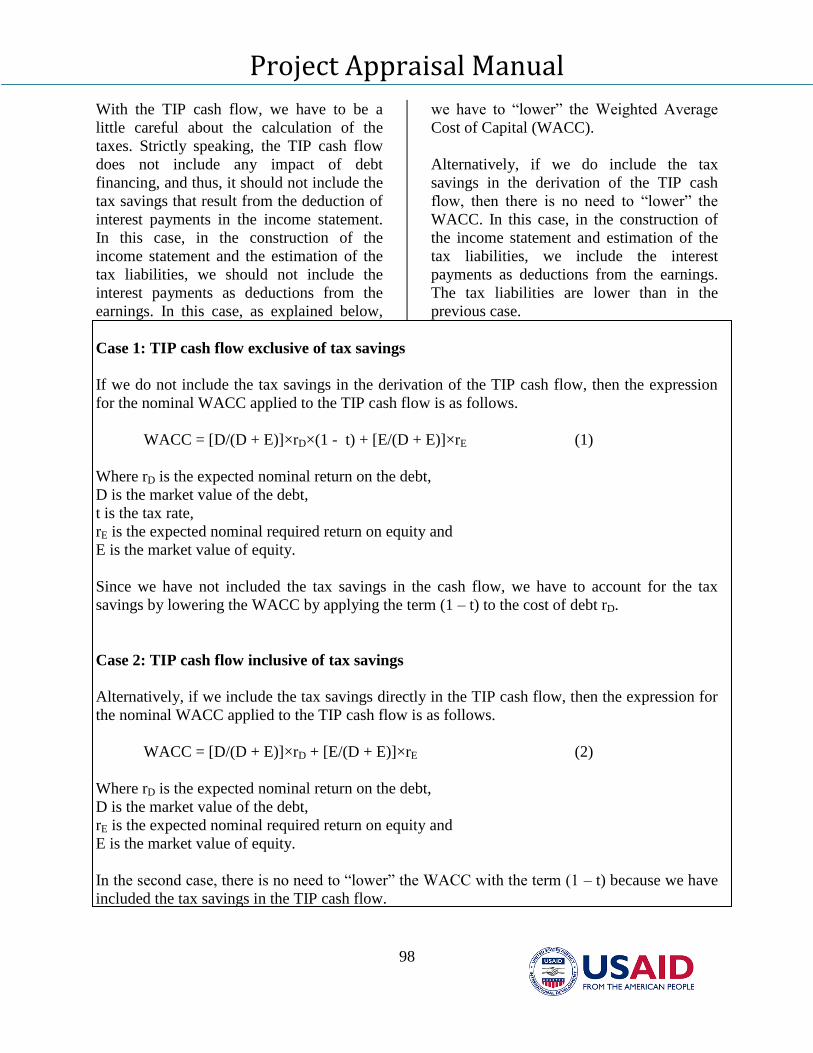
Project Appraisal Manual
98
With the TIP cash flow, we have to be a
little careful about the calculation of the
taxes. Strictly speaking, the TIP cash flow
does not include any impact of debt
financing, and thus, it should not include the
tax savings that result from the deduction of
interest payments in the income statement.
In this case, in the construction of the
income statement and the estimation of the
tax liabilities, we should not include the
interest payments as deductions from the
earnings. In this case, as explained below,
we have to “lower” the Weighted Average
Cost of Capital (WACC).
Alternatively, if we do include the tax
savings in the derivation of the TIP cash
flow, then there is no need to “lower” the
WACC. In this case, in the construction of
the income statement and estimation of the
tax liabilities, we include the interest
payments as deductions from the earnings.
The tax liabilities are lower than in the
previous case.
Case 1: TIP cash flow exclusive of tax savings
If we do not include the tax savings in the derivation of the TIP cash flow, then the expression
for the nominal WACC applied to the TIP cash flow is as follows.
WACC = [D/(D + E)]×rD×(1 - t) + [E/(D + E)]×rE (1)
Where rD is the expected nominal return on the debt,
D is the market value of the debt,
t is the tax rate,
rE is the expected nominal required return on equity and
E is the market value of equity.
Since we have not included the tax savings in the cash flow, we have to account for the tax
savings by lowering the WACC by applying the term (1 – t) to the cost of debt rD.
Case 2: TIP cash flow inclusive of tax savings
Alternatively, if we include the tax savings directly in the TIP cash flow, then the expression for
the nominal WACC applied to the TIP cash flow is as follows.
WACC = [D/(D + E)]×rD + [E/(D + E)]×rE (2)
Where rD is the expected nominal return on the debt,
D is the market value of the debt,
rE is the expected nominal required return on equity and
E is the market value of equity.
In the second case, there is no need to “lower” the WACC with the term (1 – t) because we have
included the tax savings in the TIP cash flow.
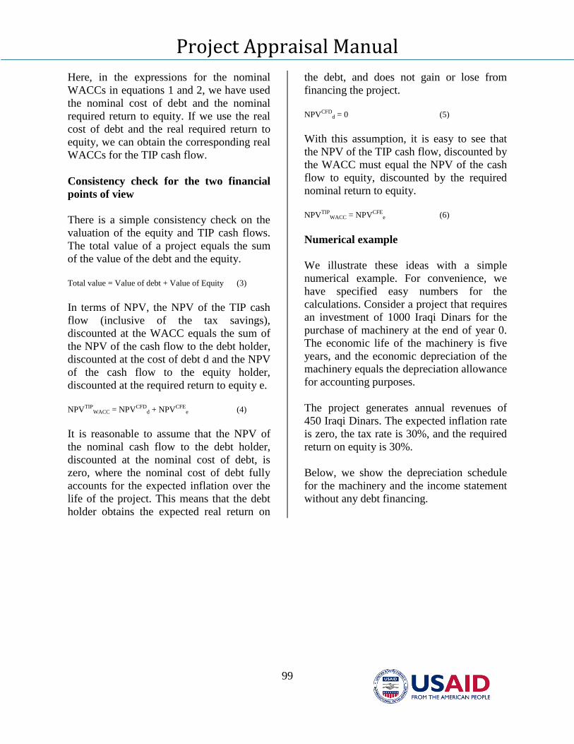
Project Appraisal Manual
99
Here, in the expressions for the nominal
WACCs in equations 1 and 2, we have used
the nominal cost of debt and the nominal
required return to equity. If we use the real
cost of debt and the real required return to
equity, we can obtain the corresponding real
WACCs for the TIP cash flow.
Consistency check for the two financial
points of view
There is a simple consistency check on the
valuation of the equity and TIP cash flows.
The total value of a project equals the sum
of the value of the debt and the equity.
Total value = Value of debt + Value of Equity (3)
In terms of NPV, the NPV of the TIP cash
flow (inclusive of the tax savings),
discounted at the WACC equals the sum of
the NPV of the cash flow to the debt holder,
discounted at the cost of debt d and the NPV
of the cash flow to the equity holder,
discounted at the required return to equity e.
NPVTIP
WACC = NPVCFDd + NPVCFE
e (4)
It is reasonable to assume that the NPV of
the nominal cash flow to the debt holder,
discounted at the nominal cost of debt, is
zero, where the nominal cost of debt fully
accounts for the expected inflation over the
life of the project. This means that the debt
holder obtains the expected real return on
the debt, and does not gain or lose from
financing the project.
NPVCFD
d = 0 (5)
With this assumption, it is easy to see that
the NPV of the TIP cash flow, discounted by
the WACC must equal the NPV of the cash
flow to equity, discounted by the required
nominal return to equity.
NPVTIP
WACC = NPVCFEe (6)
Numerical example
We illustrate these ideas with a simple
numerical example. For convenience, we
have specified easy numbers for the
calculations. Consider a project that requires
an investment of 1000 Iraqi Dinars for the
purchase of machinery at the end of year 0.
The economic life of the machinery is five
years, and the economic depreciation of the
machinery equals the depreciation allowance
for accounting purposes.
The project generates annual revenues of
450 Iraqi Dinars. The expected inflation rate
is zero, the tax rate is 30%, and the required
return on equity is 30%.
Below, we show the depreciation schedule
for the machinery and the income statement
without any debt financing.
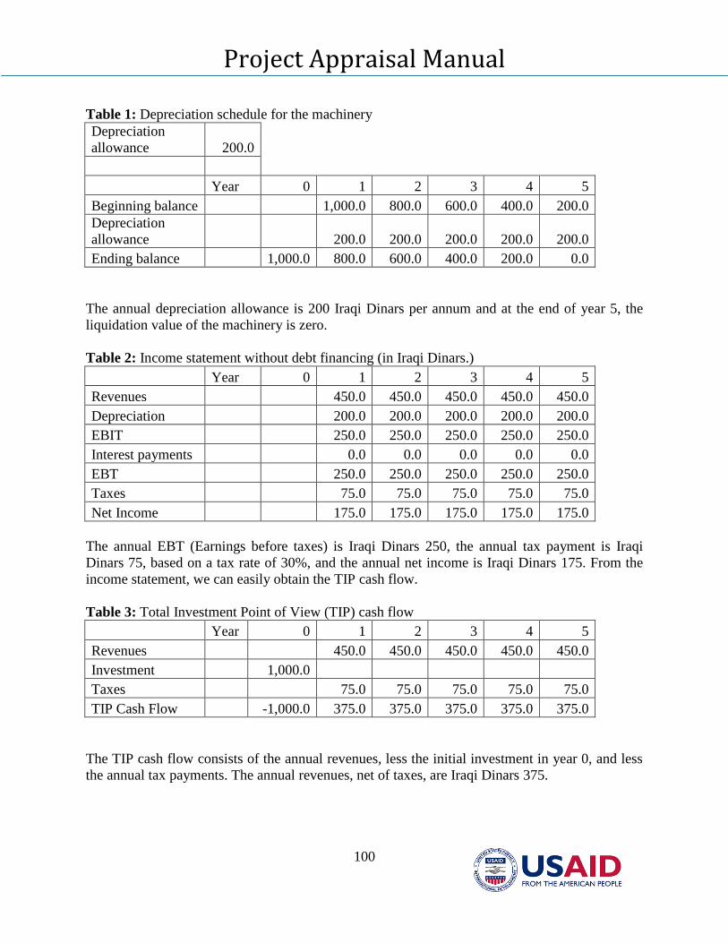
Project Appraisal Manual
100
Table 1: Depreciation schedule for the machinery
Depreciation
allowance 200.0
Year 0 1 2 3 4 5
Beginning balance 1,000.0 800.0 600.0 400.0 200.0
Depreciation
allowance 200.0 200.0 200.0 200.0 200.0
Ending balance 1,000.0 800.0 600.0 400.0 200.0 0.0
The annual depreciation allowance is 200 Iraqi Dinars per annum and at the end of year 5, the
liquidation value of the machinery is zero.
Table 2: Income statement without debt financing (in Iraqi Dinars.)
Year 0 1 2 3 4 5
Revenues 450.0 450.0 450.0 450.0 450.0
Depreciation 200.0 200.0 200.0 200.0 200.0
EBIT 250.0 250.0 250.0 250.0 250.0
Interest payments 0.0 0.0 0.0 0.0 0.0
EBT 250.0 250.0 250.0 250.0 250.0
Taxes 75.0 75.0 75.0 75.0 75.0
Net Income 175.0 175.0 175.0 175.0 175.0
The annual EBT (Earnings before taxes) is Iraqi Dinars 250, the annual tax payment is Iraqi
Dinars 75, based on a tax rate of 30%, and the annual net income is Iraqi Dinars 175. From the
income statement, we can easily obtain the TIP cash flow.
Table 3: Total Investment Point of View (TIP) cash flow
Year 0 1 2 3 4 5
Revenues 450.0 450.0 450.0 450.0 450.0
Investment 1,000.0
Taxes 75.0 75.0 75.0 75.0 75.0
TIP Cash Flow -1,000.0 375.0 375.0 375.0 375.0 375.0
The TIP cash flow consists of the annual revenues, less the initial investment in year 0, and less
the annual tax payments. The annual revenues, net of taxes, are Iraqi Dinars 375.
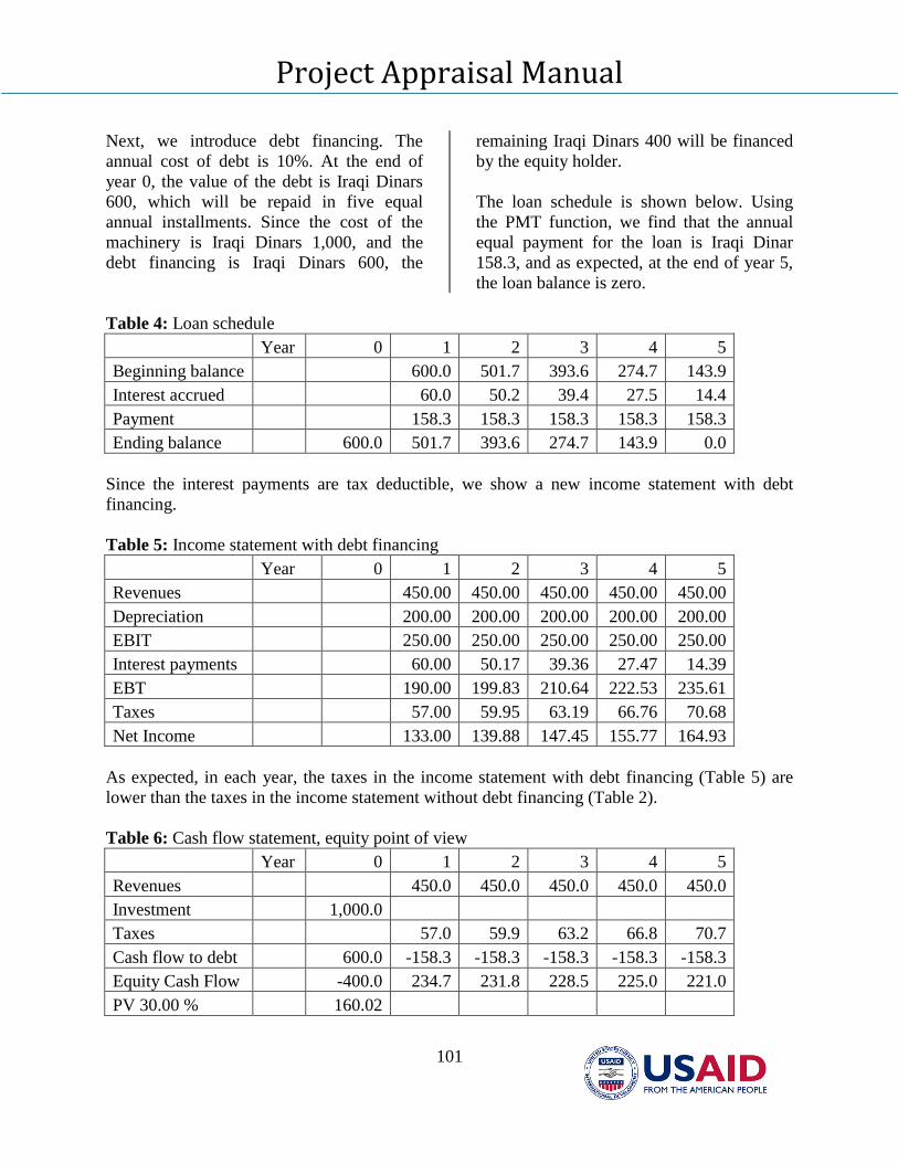
Project Appraisal Manual
101
Next, we introduce debt financing. The
annual cost of debt is 10%. At the end of
year 0, the value of the debt is Iraqi Dinars
600, which will be repaid in five equal
annual installments. Since the cost of the
machinery is Iraqi Dinars 1,000, and the
debt financing is Iraqi Dinars 600, the
remaining Iraqi Dinars 400 will be financed
by the equity holder.
The loan schedule is shown below. Using
the PMT function, we find that the annual
equal payment for the loan is Iraqi Dinar
158.3, and as expected, at the end of year 5,
the loan balance is zero.
Table 4: Loan schedule
Year 0 1 2 3 4 5
Beginning balance 600.0 501.7 393.6 274.7 143.9
Interest accrued 60.0 50.2 39.4 27.5 14.4
Payment 158.3 158.3 158.3 158.3 158.3
Ending balance 600.0 501.7 393.6 274.7 143.9 0.0
Since the interest payments are tax deductible, we show a new income statement with debt
financing.
Table 5: Income statement with debt financing
Year 0 1 2 3 4 5
Revenues 450.00 450.00 450.00 450.00 450.00
Depreciation 200.00 200.00 200.00 200.00 200.00
EBIT 250.00 250.00 250.00 250.00 250.00
Interest payments 60.00 50.17 39.36 27.47 14.39
EBT 190.00 199.83 210.64 222.53 235.61
Taxes 57.00 59.95 63.19 66.76 70.68
Net Income 133.00 139.88 147.45 155.77 164.93
As expected, in each year, the taxes in the income statement with debt financing (Table 5) are
lower than the taxes in the income statement without debt financing (Table 2).
Table 6: Cash flow statement, equity point of view
Year 0 1 2 3 4 5
Revenues 450.0 450.0 450.0 450.0 450.0
Investment 1,000.0
Taxes 57.0 59.9 63.2 66.8 70.7
Cash flow to debt 600.0 -158.3 -158.3 -158.3 -158.3 -158.3
Equity Cash Flow -400.0 234.7 231.8 228.5 225.0 221.0
PV 30.00 % 160.02

Project Appraisal Manual
102
Next, we show the cash statement from the
equity point of view. The revenues and
initial investment are the same as in Table 3.
With the interest deduction, the taxes are
lower than in Table 3. Also, now we add the
debt financing. At the end of year 0, the loan
is a cash inflow, and the repayments in years
1 to 5 are cash outflows. With respect to the
end of year 0, the net present value (NPV) of
the equity cash flow, discounted at the
required return to equity of 30%, is 160.02.
Project Appraisal Manual
103
Annex I: Conducting Financial Analysis in Nominal Prices
The effects of inflation on a project's
financial condition include:
(1) Direct impacts from changes in
investment financing, cash balances,
accounts receivable, accounts payable, and
nominal interest rates,
(2) Tax impacts including interest expenses,
depreciation and inventories, and
(3) The impact on the market exchange rate.
Inflation alters the amount and timing of the
financial gains and losses of the various
parties involved in a project including the
owner(s), the lender(s) and the government.
Correctly accounting for those changes is
necessary to determine how the overall
project and each of the interested parties are
affected by different levels of inflation.
1. Direct Effects
(i) Investment Financing
When estimating the amount of financing an
investment project requires, it is important
to distinguish between two types of cost
increases. First, there are cost over-runs
which are caused by incorrect estimates of
the quantities of materials required or
changes in the real prices of those materials.
Second, there is cost escalation which is
attributable to the general price level
inflation. The “escalation” of costs that
stems from pure price inflation should be
recognized as normal and, if possible,
should be anticipated and included in the
project appraisal. If the project requires a
loan or equity financing for future outlays, it
should be recognized that the amount of
financing needed will be affected by the
amount of price inflation that takes place
during the time of construction. Cost
increases attributable to inflation are not
overruns of real costs; therefore, additional
borrowing that simply reflects the rise in the
general level of prices should be planned
for. If this condition is not adequately
planned for at the appraisal stage, the project
may experience a liquidity crisis or
insolvency due to inadequate financing.
Table A-1 demonstrates the effects of
inflation on investment financing. All
values are given in Iraqi Dinars. The project
will be built during the first two time
periods, operate for following four, and then
be liquidated in the final time period. The
total cost of construction will be capitalized
at the end of the second period to determine
the amount to be depreciated. Loans are
obtained for 50% of the investment in fixed
assets. Loan financing will have a nominal
interest rate of 5 percent per period if there
is no inflation, and interest will begin
accruing during the construction period.
The loan principal will be repaid at the end
of the last operating year of the project,
period 5. The remainder of the financing
requirements is covered by the owners'
equity.
In this project an investment of 5000 Iraqi
Dinars is made in fixed assets in year 0, and
if there is no inflation, a further 5000 Iraqi
Dinars is made in year 1. If there is 25%
inflation a year, the initial year's investment
does not change, however the nominal
investment undertaken in year 1 increases to
6,250 Iraqi Dinars.
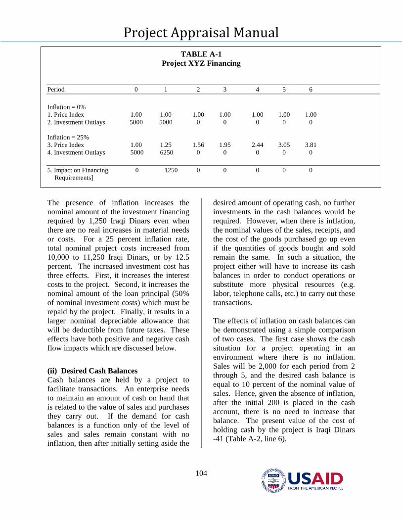
Project Appraisal Manual
104
TABLE A-1
Project XYZ Financing
Period 0 1 2 3 4 5 6
Inflation = 0%
1. Price Index 1.00 1.00 1.00 1.00 1.00 1.00 1.00
2. Investment Outlays 5000 5000 0 0 0 0 0
Inflation = 25%
3. Price Index 1.00 1.25 1.56 1.95 2.44 3.05 3.81
4. Investment Outlays 5000 6250 0 0 0 0 0
5. Impact on Financing 0 1250 0 0 0 0 0
Requirements]
The presence of inflation increases the
nominal amount of the investment financing
required by 1,250 Iraqi Dinars even when
there are no real increases in material needs
or costs. For a 25 percent inflation rate,
total nominal project costs increased from
10,000 to 11,250 Iraqi Dinars, or by 12.5
percent. The increased investment cost has
three effects. First, it increases the interest
costs to the project. Second, it increases the
nominal amount of the loan principal (50%
of nominal investment costs) which must be
repaid by the project. Finally, it results in a
larger nominal depreciable allowance that
will be deductible from future taxes. These
effects have both positive and negative cash
flow impacts which are discussed below.
(ii) Desired Cash Balances
Cash balances are held by a project to
facilitate transactions. An enterprise needs
to maintain an amount of cash on hand that
is related to the value of sales and purchases
they carry out. If the demand for cash
balances is a function only of the level of
sales and sales remain constant with no
inflation, then after initially setting aside the
desired amount of operating cash, no further
investments in the cash balances would be
required. However, when there is inflation,
the nominal values of the sales, receipts, and
the cost of the goods purchased go up even
if the quantities of goods bought and sold
remain the same. In such a situation, the
project either will have to increase its cash
balances in order to conduct operations or
substitute more physical resources (e.g.
labor, telephone calls, etc.) to carry out these
transactions.
The effects of inflation on cash balances can
be demonstrated using a simple comparison
of two cases. The first case shows the cash
situation for a project operating in an
environment where there is no inflation.
Sales will be 2,000 for each period from 2
through 5, and the desired cash balance is
equal to 10 percent of the nominal value of
sales. Hence, given the absence of inflation,
after the initial 200 is placed in the cash
account, there is no need to increase that
balance. The present value of the cost of
holding cash by the project is Iraqi Dinars
-41 (Table A-2, line 6).
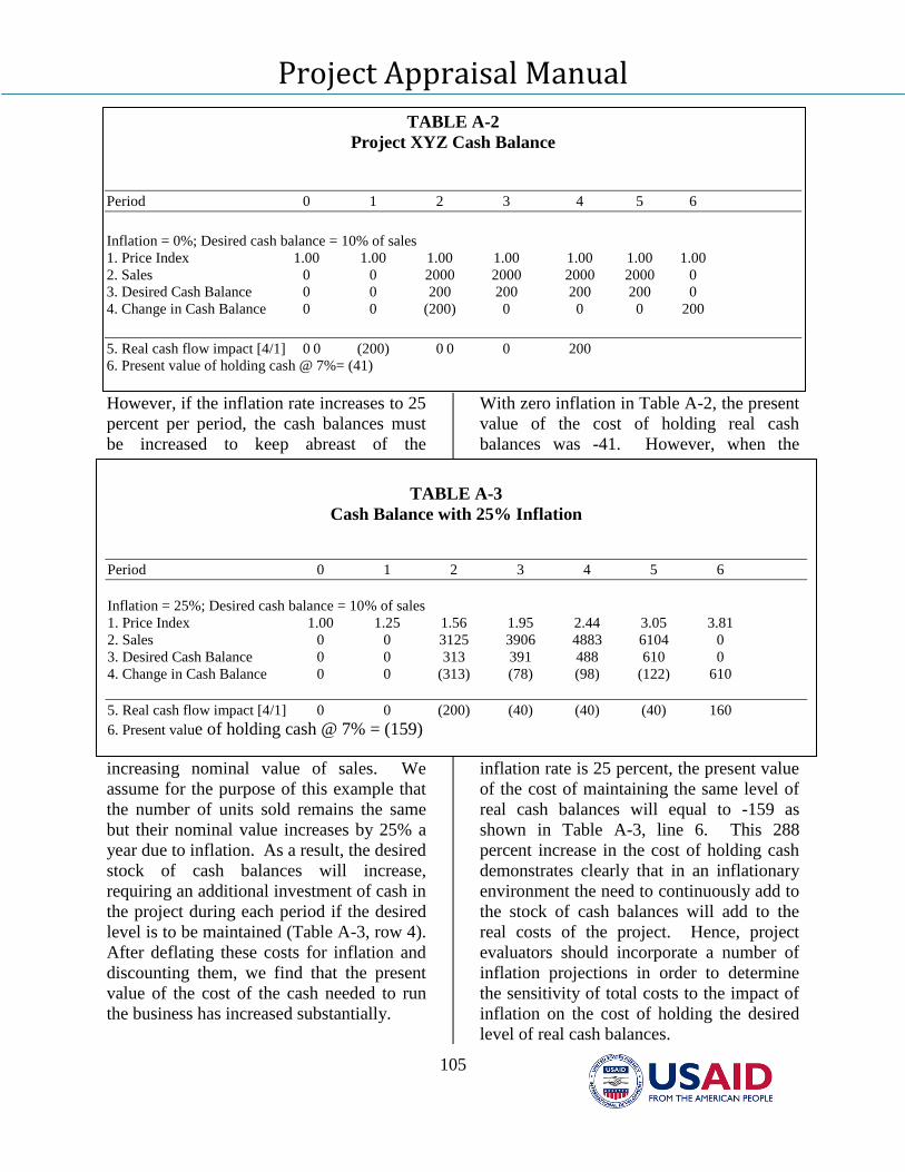
Project Appraisal Manual
105
TABLE A-2
Project XYZ Cash Balance
Period 0 1 2 3 4 5 6
Inflation = 0%; Desired cash balance = 10% of sales
1. Price Index 1.00 1.00 1.00 1.00 1.00 1.00 1.00
2. Sales 0 0 2000 2000 2000 2000 0
3. Desired Cash Balance 0 0 200 200 200 200 0
4. Change in Cash Balance 0 0 (200) 0 0 0 200
5. Real cash flow impact [4/1] 0 0 (200) 0 0 0 200
6. Present value of holding cash @ 7%= (41)
However, if the inflation rate increases to 25
percent per period, the cash balances must
be increased to keep abreast of the
increasing nominal value of sales. We
assume for the purpose of this example that
the number of units sold remains the same
but their nominal value increases by 25% a
year due to inflation. As a result, the desired
stock of cash balances will increase,
requiring an additional investment of cash in
the project during each period if the desired
level is to be maintained (Table A-3, row 4).
After deflating these costs for inflation and
discounting them, we find that the present
value of the cost of the cash needed to run
the business has increased substantially.
With zero inflation in Table A-2, the present
value of the cost of holding real cash
balances was -41. However, when the
inflation rate is 25 percent, the present value
of the cost of maintaining the same level of
real cash balances will equal to -159 as
shown in Table A-3, line 6. This 288
percent increase in the cost of holding cash
demonstrates clearly that in an inflationary
environment the need to continuously add to
the stock of cash balances will add to the
real costs of the project. Hence, project
evaluators should incorporate a number of
inflation projections in order to determine
the sensitivity of total costs to the impact of
inflation on the cost of holding the desired
level of real cash balances.
TABLE A-3
Cash Balance with 25% Inflation
Period 0 1 2 3 4 5 6
Inflation = 25%; Desired cash balance = 10% of sales
1. Price Index 1.00 1.25 1.56 1.95 2.44 3.05 3.81
2. Sales 0 0 3125 3906 4883 6104 0
3. Desired Cash Balance 0 0 313 391 488 610 0
4. Change in Cash Balance 0 0 (313) (78) (98) (122) 610
5. Real cash flow impact [4/1] 0 0 (200) (40) (40) (40) 160
6. Present value of holding cash @ 7% = (159)
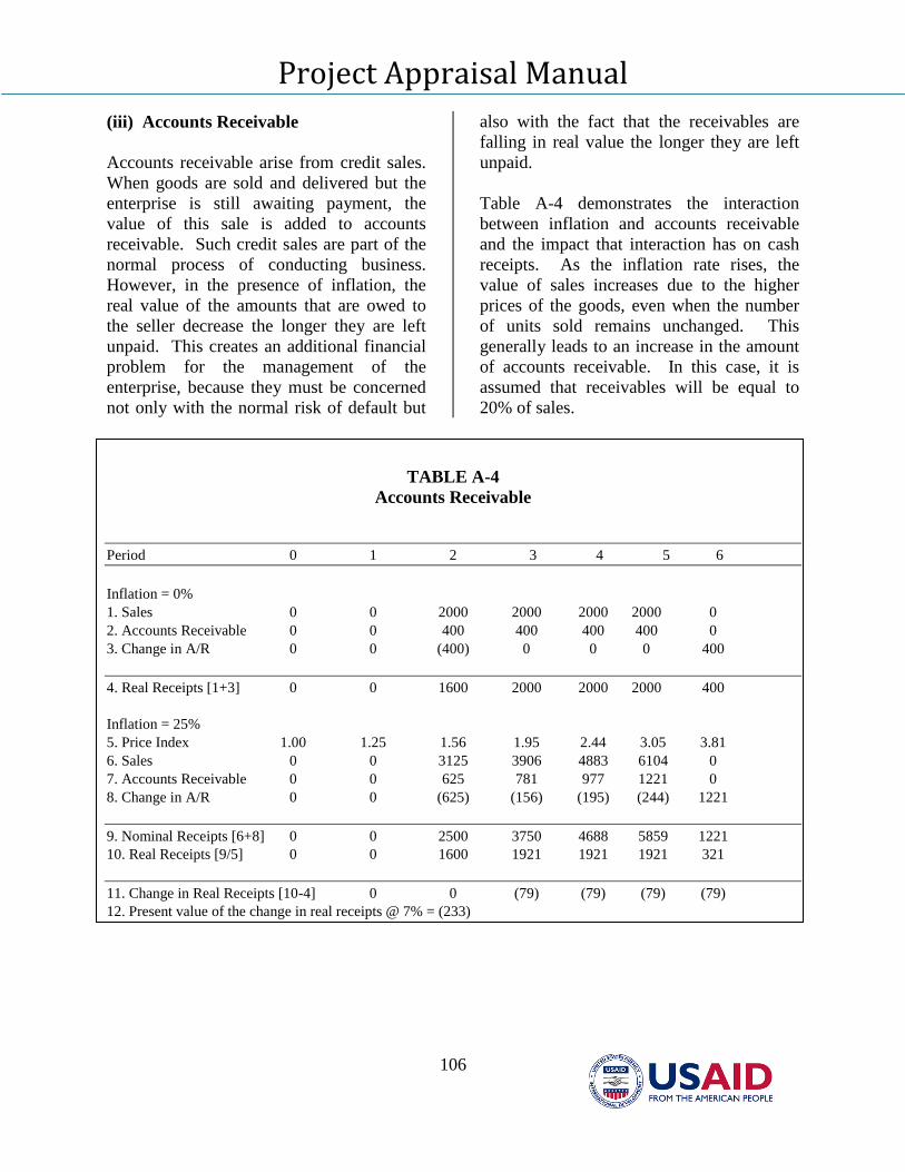
Project Appraisal Manual
106
(iii) Accounts Receivable
Accounts receivable arise from credit sales.
When goods are sold and delivered but the
enterprise is still awaiting payment, the
value of this sale is added to accounts
receivable. Such credit sales are part of the
normal process of conducting business.
However, in the presence of inflation, the
real value of the amounts that are owed to
the seller decrease the longer they are left
unpaid. This creates an additional financial
problem for the management of the
enterprise, because they must be concerned
not only with the normal risk of default but
also with the fact that the receivables are
falling in real value the longer they are left
unpaid.
Table A-4 demonstrates the interaction
between inflation and accounts receivable
and the impact that interaction has on cash
receipts. As the inflation rate rises, the
value of sales increases due to the higher
prices of the goods, even when the number
of units sold remains unchanged. This
generally leads to an increase in the amount
of accounts receivable. In this case, it is
assumed that receivables will be equal to
20% of sales.
TABLE A-4
Accounts Receivable
Period 0 1 2 3 4 5 6
Inflation = 0%
1. Sales 0 0 2000 2000 2000 2000 0
2. Accounts Receivable 0 0 400 400 400 400 0
3. Change in A/R 0 0 (400) 0 0 0 400
4. Real Receipts [1+3] 0 0 1600 2000 2000 2000 400
Inflation = 25%
5. Price Index 1.00 1.25 1.56 1.95 2.44 3.05 3.81
6. Sales 0 0 3125 3906 4883 6104 0
7. Accounts Receivable 0 0 625 781 977 1221 0
8. Change in A/R 0 0 (625) (156) (195) (244) 1221
9. Nominal Receipts [6+8] 0 0 2500 3750 4688 5859 1221
10. Real Receipts [9/5] 0 0 1600 1921 1921 1921 321
11. Change in Real Receipts [10-4] 0 0 (79) (79) (79) (79)
12. Present value of the change in real receipts @ 7% = (233)
Project Appraisal Manual
107
In spite of the fact that the nominal value of
sales increases each period when there is 25
percent inflation, Table A-4 demonstrates
that the present value of the real receipts for
this project decreases by 233 due to the
higher rate of inflation. This is because
inflation causes the real value of outstanding
trade credit to fall. When this situation
arises, businesses selling goods or services
(the project in this case) will attempt to
reduce the length of the terms they give for
trade credit, while businesses purchasing the
product will have an additional incentive to
delay payment. Therefore, it is important to
include in a project evaluation the
interaction of inflation and accounts
receivable to determine how the real receipts
of the business are affected by inflation. (iv) Accounts’ Payable
Accounts payable represent the amount of
money owed by a business to others for
goods or services already purchased and
delivered. When there is inflation, the buyer
with the accounts payable benefits from
having an outstanding balance because the
real value of the obligation is falling during
the period of time prior to the payment.
This is simply the other side of the impact of
inflation on accounts receivable because one
enterprise’s accounts receivable is another’s
accounts payable.
Table A-5 shows how inflation affects a
project’s financial situation when accounts
payable are equal to 25% of annual
purchases. Once again, we see that inflation
increases the nominal value of purchases
which leads to greater accounts payable as
well.
The increased rate of inflation results in a
net decrease of 155 in the present value of
real expenditures. As shown in line 6,
inflation increases the nominal value of
purchases, and creates a corresponding
increase in nominal accounts payable in line
7. When converted to real expenditures, the
buyer (the project in this case) benefits from
the effects of inflation on accounts payable
and will have a lower overall level of
expenditure, as shown in Table A-5, row 11.
This gives the buyer an incentive to extend
the terms of the accounts payable to benefit
from their falling real value. Hence, in the
presence of inflation, the longer the
outstanding accounts payable are held
before being paid, the greater the benefit
accruing to the buyer.
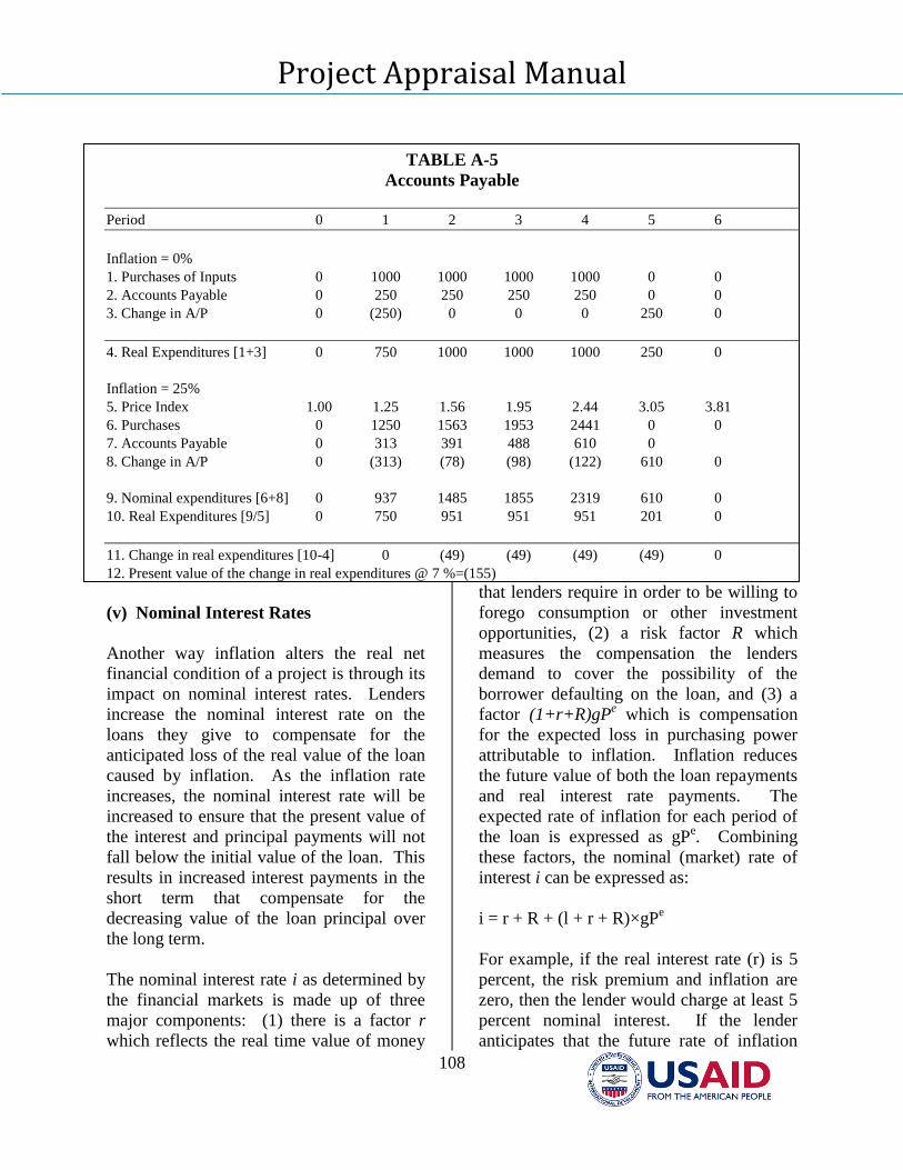
Project Appraisal Manual
108
TABLE A-5
Accounts Payable
Period 0 1 2 3 4 5 6
Inflation = 0%
1. Purchases of Inputs 0 1000 1000 1000 1000 0 0
2. Accounts Payable 0 250 250 250 250 0 0
3. Change in A/P 0 (250) 0 0 0 250 0
4. Real Expenditures [1+3] 0 750 1000 1000 1000 250 0
Inflation = 25%
5. Price Index 1.00 1.25 1.56 1.95 2.44 3.05 3.81
6. Purchases 0 1250 1563 1953 2441 0 0
7. Accounts Payable 0 313 391 488 610 0
8. Change in A/P 0 (313) (78) (98) (122) 610 0
9. Nominal expenditures [6+8] 0 937 1485 1855 2319 610 0
10. Real Expenditures [9/5] 0 750 951 951 951 201 0
11. Change in real expenditures [10-4] 0 (49) (49) (49) (49) 0
12. Present value of the change in real expenditures @ 7 %=(155)
(v) Nominal Interest Rates
Another way inflation alters the real net
financial condition of a project is through its
impact on nominal interest rates. Lenders
increase the nominal interest rate on the
loans they give to compensate for the
anticipated loss of the real value of the loan
caused by inflation. As the inflation rate
increases, the nominal interest rate will be
increased to ensure that the present value of
the interest and principal payments will not
fall below the initial value of the loan. This
results in increased interest payments in the
short term that compensate for the
decreasing value of the loan principal over
the long term.
The nominal interest rate i as determined by
the financial markets is made up of three
major components: (1) there is a factor r
which reflects the real time value of money
that lenders require in order to be willing to
forego consumption or other investment
opportunities, (2) a risk factor R which
measures the compensation the lenders
demand to cover the possibility of the
borrower defaulting on the loan, and (3) a
factor (1+r+R)gPe which is compensation
for the expected loss in purchasing power
attributable to inflation. Inflation reduces
the future value of both the loan repayments
and real interest rate payments. The
expected rate of inflation for each period of
the loan is expressed as gPe. Combining
these factors, the nominal (market) rate of
interest i can be expressed as:
i = r + R + (l + r + R)×gPe
For example, if the real interest rate (r) is 5
percent, the risk premium and inflation are
zero, then the lender would charge at least 5
percent nominal interest. If the lender
anticipates that the future rate of inflation
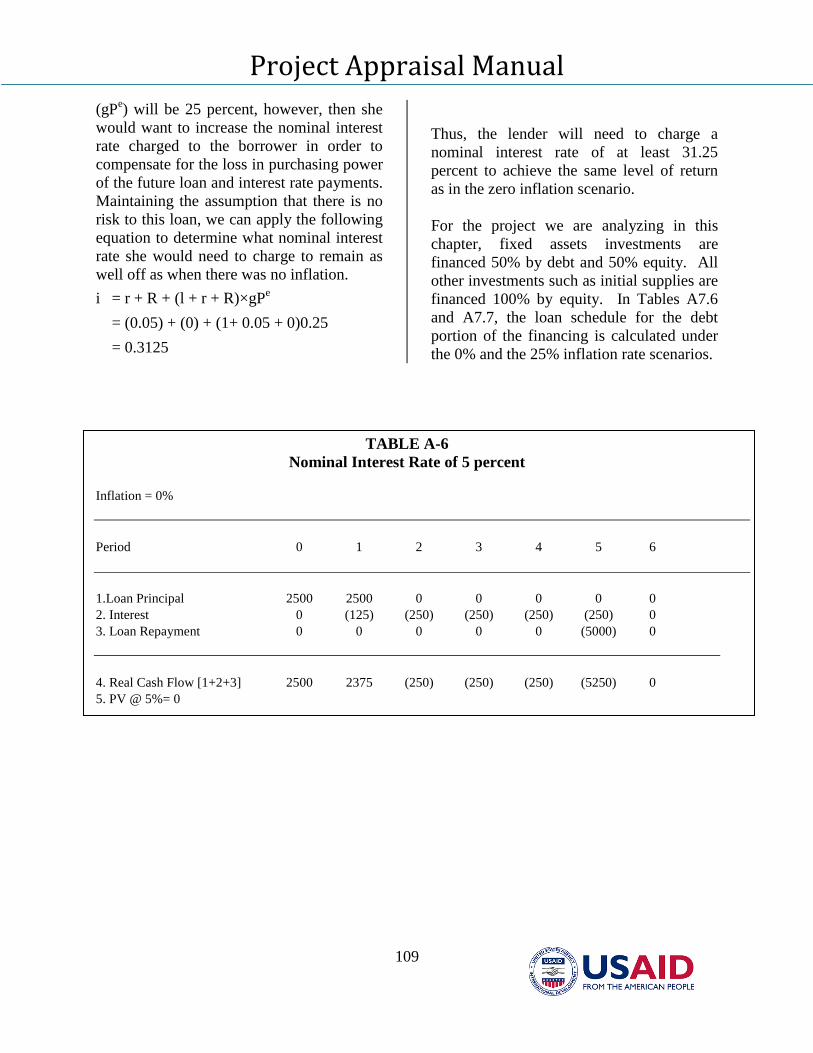
Project Appraisal Manual
109
(gPe) will be 25 percent, however, then she
would want to increase the nominal interest
rate charged to the borrower in order to
compensate for the loss in purchasing power
of the future loan and interest rate payments.
Maintaining the assumption that there is no
risk to this loan, we can apply the following
equation to determine what nominal interest
rate she would need to charge to remain as
well off as when there was no inflation.
i = r + R + (l + r + R)×gPe
= (0.05) + (0) + (1+ 0.05 + 0)0.25
= 0.3125
Thus, the lender will need to charge a
nominal interest rate of at least 31.25
percent to achieve the same level of return
as in the zero inflation scenario.
For the project we are analyzing in this
chapter, fixed assets investments are
financed 50% by debt and 50% equity. All
other investments such as initial supplies are
financed 100% by equity. In Tables A7.6
and A7.7, the loan schedule for the debt
portion of the financing is calculated under
the 0% and the 25% inflation rate scenarios.
TABLE A-6
Nominal Interest Rate of 5 percent
Inflation = 0%
Period 0 1 2 3 4 5 6
1.Loan Principal 2500 2500 0 0 0 0 0
2. Interest 0 (125) (250) (250) (250) (250) 0
3. Loan Repayment 0 0 0 0 0 (5000) 0
4. Real Cash Flow [1+2+3] 2500 2375 (250) (250) (250) (5250) 0
5. PV @ 5%= 0
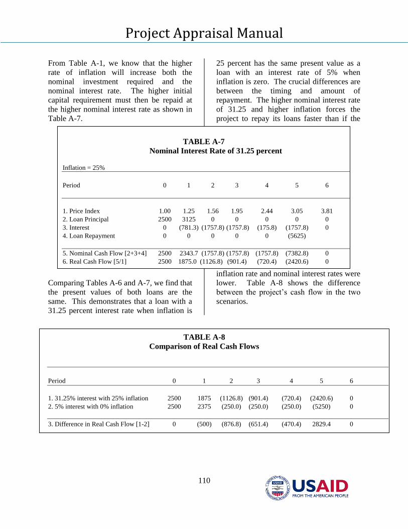
Project Appraisal Manual
110
From Table A-1, we know that the higher
rate of inflation will increase both the
nominal investment required and the
nominal interest rate. The higher initial
capital requirement must then be repaid at
the higher nominal interest rate as shown in
Table A-7.
Comparing Tables A-6 and A-7, we find that
the present values of both loans are the
same. This demonstrates that a loan with a
31.25 percent interest rate when inflation is
25 percent has the same present value as a
loan with an interest rate of 5% when
inflation is zero. The crucial differences are
between the timing and amount of
repayment. The higher nominal interest rate
of 31.25 and higher inflation forces the
project to repay its loans faster than if the
inflation rate and nominal interest rates were
lower. Table A-8 shows the difference
between the project’s cash flow in the two
scenarios.
TABLE A-8
Comparison of Real Cash Flows
Period 0 1 2 3 4 5 6
1. 31.25% interest with 25% inflation 2500 1875 (1126.8) (901.4) (720.4) (2420.6) 0
2. 5% interest with 0% inflation 2500 2375 (250.0) (250.0) (250.0) (5250) 0
3. Difference in Real Cash Flow [1-2] 0 (500) (876.8) (651.4) (470.4) 2829.4 0
TABLE A-7
Nominal Interest Rate of 31.25 percent
Inflation = 25%
Period 0 1 2 3 4 5 6
1. Price Index 1.00 1.25 1.56 1.95 2.44 3.05 3.81
2. Loan Principal 2500 3125 0 0 0 0 0
3. Interest 0 (781.3) (1757.8) (1757.8) (175.8) (1757.8) 0
4. Loan Repayment 0 0 0 0 0 (5625)
5. Nominal Cash Flow [2+3+4] 2500 2343.7 (1757.8) (1757.8) (1757.8) (7382.8) 0
6. Real Cash Flow [5/1] 2500 1875.0 (1126.8) (901.4) (720.4) (2420.6) 0
7. PV @ 5%= 0
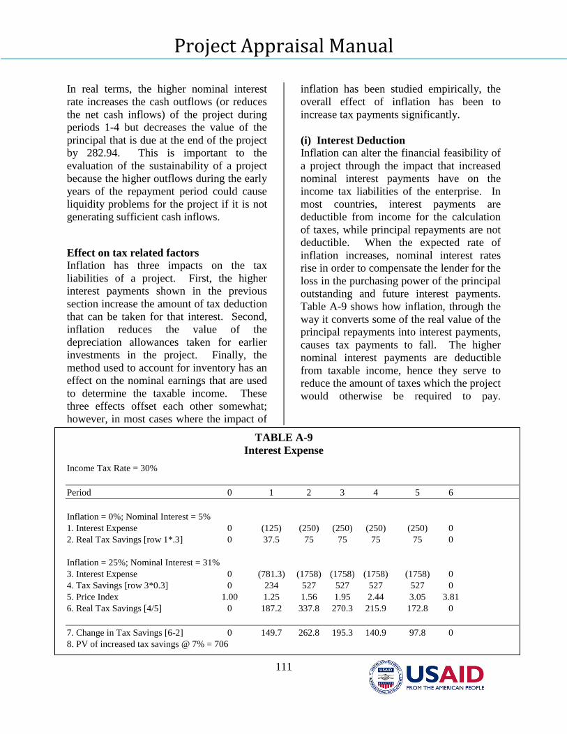
Project Appraisal Manual
111
In real terms, the higher nominal interest
rate increases the cash outflows (or reduces
the net cash inflows) of the project during
periods 1-4 but decreases the value of the
principal that is due at the end of the project
by 282.94. This is important to the
evaluation of the sustainability of a project
because the higher outflows during the early
years of the repayment period could cause
liquidity problems for the project if it is not
generating sufficient cash inflows. Effect on tax related factors
Inflation has three impacts on the tax
liabilities of a project. First, the higher
interest payments shown in the previous
section increase the amount of tax deduction
that can be taken for that interest. Second,
inflation reduces the value of the
depreciation allowances taken for earlier
investments in the project. Finally, the
method used to account for inventory has an
effect on the nominal earnings that are used
to determine the taxable income. These
three effects offset each other somewhat;
however, in most cases where the impact of
inflation has been studied empirically, the
overall effect of inflation has been to
increase tax payments significantly.
(i) Interest Deduction
Inflation can alter the financial feasibility of
a project through the impact that increased
nominal interest payments have on the
income tax liabilities of the enterprise. In
most countries, interest payments are
deductible from income for the calculation
of taxes, while principal repayments are not
deductible. When the expected rate of
inflation increases, nominal interest rates
rise in order to compensate the lender for the
loss in the purchasing power of the principal
outstanding and future interest payments.
Table A-9 shows how inflation, through the
way it converts some of the real value of the
principal repayments into interest payments,
causes tax payments to fall. The higher
nominal interest payments are deductible
from taxable income, hence they serve to
reduce the amount of taxes which the project
would otherwise be required to pay.
TABLE A-9
Interest Expense
Income Tax Rate = 30%
Period 0 1 2 3 4 5 6
Inflation = 0%; Nominal Interest = 5%
1. Interest Expense 0 (125) (250) (250) (250) (250) 0
2. Real Tax Savings [row 1*.3] 0 37.5 75 75 75 75 0
Inflation = 25%; Nominal Interest = 31%
3. Interest Expense 0 (781.3) (1758) (1758) (1758) (1758) 0
4. Tax Savings [row 3*0.3] 0 234 527 527 527 527 0
5. Price Index 1.00 1.25 1.56 1.95 2.44 3.05 3.81
6. Real Tax Savings [4/5] 0 187.2 337.8 270.3 215.9 172.8 0
7. Change in Tax Savings [6-2] 0 149.7 262.8 195.3 140.9 97.8 0
8. PV of increased tax savings @ 7% = 706
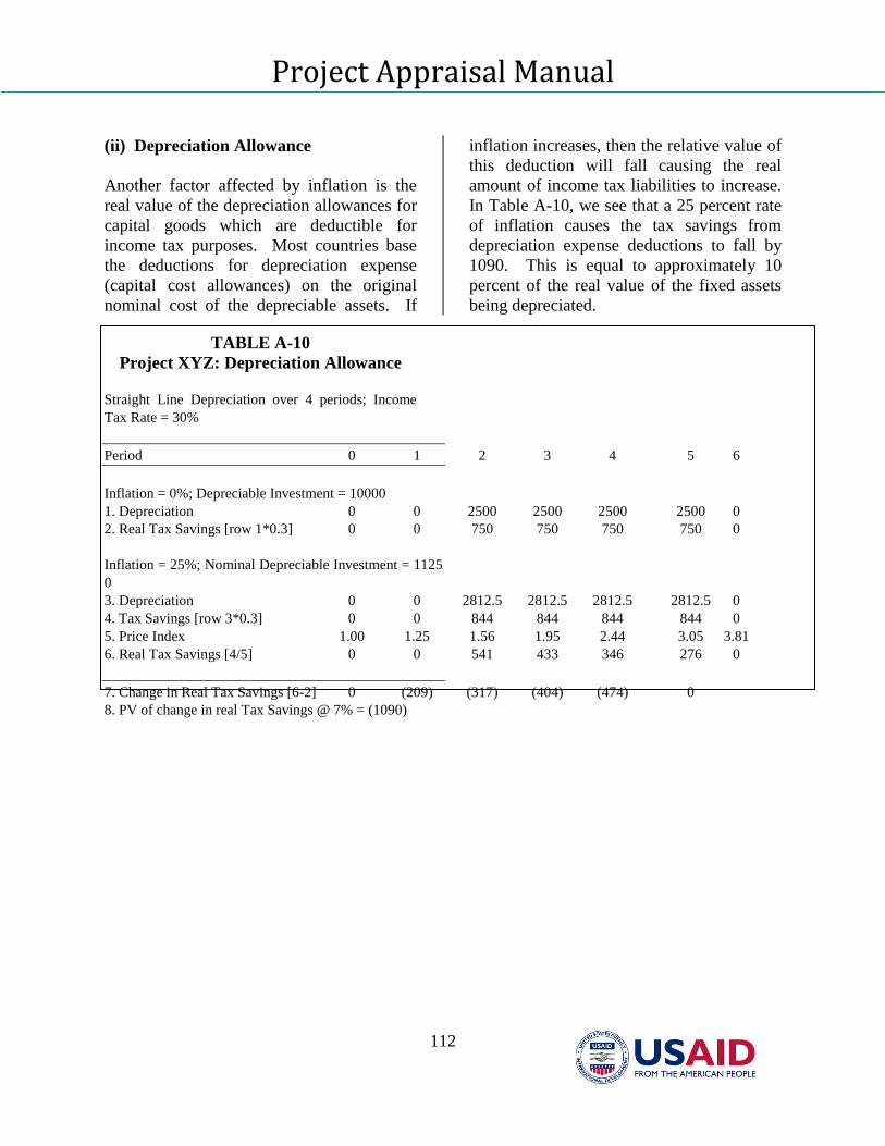
Project Appraisal Manual
112
(ii) Depreciation Allowance
Another factor affected by inflation is the
real value of the depreciation allowances for
capital goods which are deductible for
income tax purposes. Most countries base
the deductions for depreciation expense
(capital cost allowances) on the original
nominal cost of the depreciable assets. If
inflation increases, then the relative value of
this deduction will fall causing the real
amount of income tax liabilities to increase.
In Table A-10, we see that a 25 percent rate
of inflation causes the tax savings from
depreciation expense deductions to fall by
1090. This is equal to approximately 10
percent of the real value of the fixed assets
being depreciated.
TABLE A-10
Project XYZ: Depreciation Allowance
Straight Line Depreciation over 4 periods; Income
Tax Rate = 30%
Period 0 1 2 3 4 5 6
Inflation = 0%; Depreciable Investment = 10000
1. Depreciation 0 0 2500 2500 2500 2500 0
2. Real Tax Savings [row 1*0.3] 0 0 750 750 750 750 0
Inflation = 25%; Nominal Depreciable Investment = 1125
0
3. Depreciation 0 0 2812.5 2812.5 2812.5 2812.5 0
4. Tax Savings [row 3*0.3] 0 0 844 844 844 844 0
5. Price Index 1.00 1.25 1.56 1.95 2.44 3.05 3.81
6. Real Tax Savings [4/5] 0 0 541 433 346 276 0
7. Change in Real Tax Savings [6-2] 0 (209) (317) (404) (474) 0
8. PV of change in real Tax Savings @ 7% = (1090)
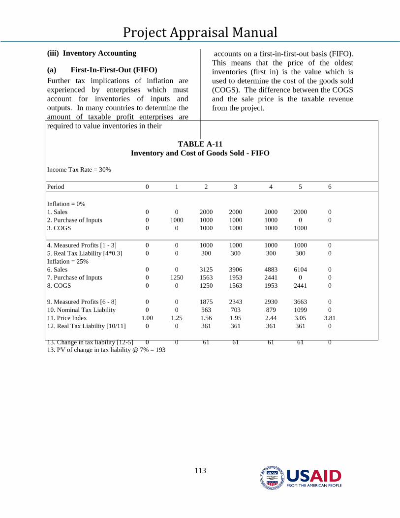
Project Appraisal Manual
113
(iii) Inventory Accounting
(a) First-In-First-Out (FIFO)
Further tax implications of inflation are
experienced by enterprises which must
account for inventories of inputs and
outputs. In many countries to determine the
amount of taxable profit enterprises are
required to value inventories in their
accounts on a first-in-first-out basis (FIFO).
This means that the price of the oldest
inventories (first in) is the value which is
used to determine the cost of the goods sold
(COGS). The difference between the COGS
and the sale price is the taxable revenue
from the project.
TABLE A-11
Inventory and Cost of Goods Sold - FIFO
Income Tax Rate = 30%
Period 0 1 2 3 4 5 6
Inflation = 0%
1. Sales 0 0 2000 2000 2000 2000 0
2. Purchase of Inputs 0 1000 1000 1000 1000 0 0
3. COGS 0 0 1000 1000 1000 1000
4. Measured Profits [1 - 3] 0 0 1000 1000 1000 1000 0
5. Real Tax Liability [4*0.3] 0 0 300 300 300 300 0
Inflation = 25%
6. Sales 0 0 3125 3906 4883 6104 0
7. Purchase of Inputs 0 1250 1563 1953 2441 0 0
8. COGS 0 0 1250 1563 1953 2441 0
9. Measured Profits [6 - 8] 0 0 1875 2343 2930 3663 0
10. Nominal Tax Liability 0 0 563 703 879 1099 0
11. Price Index 1.00 1.25 1.56 1.95 2.44 3.05 3.81
12. Real Tax Liability [10/11] 0 0 361 361 361 361 0
13. Change in tax liability [12-5] 0 0 61 61 61 61 0
13. PV of change in tax liability @ 7% = 193
Project Appraisal Manual
114
Taxable revenue generally increases by the
rate of inflation because sale prices are
affected immediately by the rate of inflation,
while the costs of goods sold from
inventories are valued using prices of a
previous period when the nominal prices
were presumably lower. For example, if the
project has a one year inventory of final
goods at the beginning of the year and the
inflation rate for that year is 25 percent, then
nominal cost prices of the goods sold will be
25 percent lower than their selling prices
one year later, even if no profit margin is
added. The result is that the measured
profits are artificially inflated which
increases the tax burden in both nominal and
real terms.17
From Table A-11, lines 1-14,
we see that by increasing the rate of inflation
from 0 to 25 percent, the present value of
real tax payments increases by 193.
(b) Last-In-First-Out (LIFO)
Another method for accounting for the cost
of goods sold is known as last-in-first-out
(LIFO). As the name implies, the most
recent goods purchased (last in) are used to
measure the cost of goods sold (first out),
and the prices of the project inputs are
generally increasing at the same rate of
inflation as the outputs sold. During the
production cycle of a project, this is a
benefit because the profits are not increased
artificially by the presence of inflation. It
also means that taxes will be lower as a
result. However, LIFO has a negative
17
. This occurs because, in a period of rapid
inflation, the historical cost of inventories now being
used in production will be substantially less than the
current replacement cost of these items. If taxable
income is calculated using the historical cost of the
inventory items, the real cost of goods will be
underestimated and taxable income will be
overestimated. Therefore, real income tax liabilities
will be greater than they would be if no inflation had
existed.
aspect as well because as the activity winds
down, or the level of inventories is reduced
due to business conditions, the lower prices
of the goods that were purchased in earlier
years are now used to calculate the cost of
goods sold, resulting in inflated profits and
increased taxes as shown in Table A-12, row
13 - period 5.
The LIFO system for accounting for cost of
goods sold allowed tax liabilities to remain
unaltered until period 5. As the project
winds down, the prices used to calculate the
COGS for that period are now from period
one. Hence, with 25 percent inflation profits
in period five will be greatly inflated,
causing the tax burden to increase in real
terms by 177 (line 13 - period 5) over the no
inflation scenario.
Comparing the effects of inflation on the tax
liability in the FIFO and LIFO accounting
systems, we see that in both cases, inflation
increased the taxes. With FIFO and 25
percent inflation the present value of the tax
liability increased by 193 (Table A-11), and
with LIFO, the present value increased by
126 (Table A-12).
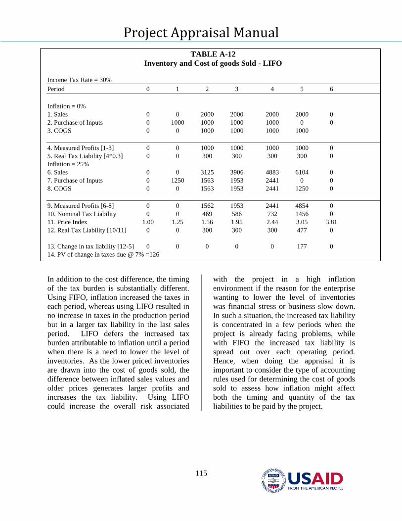
Project Appraisal Manual
115
TABLE A-12
Inventory and Cost of goods Sold - LIFO
Income Tax Rate = 30%
Period 0 1 2 3 4 5 6
Inflation = 0%
1. Sales 0 0 2000 2000 2000 2000 0
2. Purchase of Inputs 0 1000 1000 1000 1000 0 0
3. COGS 0 0 1000 1000 1000 1000
4. Measured Profits [1-3] 0 0 1000 1000 1000 1000 0
5. Real Tax Liability [4*0.3] 0 0 300 300 300 300 0
Inflation = 25%
6. Sales 0 0 3125 3906 4883 6104 0
7. Purchase of Inputs 0 1250 1563 1953 2441 0 0
8. COGS 0 0 1563 1953 2441 1250 0
9. Measured Profits [6-8] 0 0 1562 1953 2441 4854 0
10. Nominal Tax Liability 0 0 469 586 732 1456 0
11. Price Index 1.00 1.25 1.56 1.95 2.44 3.05 3.81
12. Real Tax Liability [10/11] 0 0 300 300 300 477 0
13. Change in tax liability [12-5] 0 0 0 0 0 177 0
14. PV of change in taxes due @ 7% =126
In addition to the cost difference, the timing
of the tax burden is substantially different.
Using FIFO, inflation increased the taxes in
each period, whereas using LIFO resulted in
no increase in taxes in the production period
but in a larger tax liability in the last sales
period. LIFO defers the increased tax
burden attributable to inflation until a period
when there is a need to lower the level of
inventories. As the lower priced inventories
are drawn into the cost of goods sold, the
difference between inflated sales values and
older prices generates larger profits and
increases the tax liability. Using LIFO
could increase the overall risk associated
with the project in a high inflation
environment if the reason for the enterprise
wanting to lower the level of inventories
was financial stress or business slow down.
In such a situation, the increased tax liability
is concentrated in a few periods when the
project is already facing problems, while
with FIFO the increased tax liability is
spread out over each operating period.
Hence, when doing the appraisal it is
important to consider the type of accounting
rules used for determining the cost of goods
sold to assess how inflation might affect
both the timing and quantity of the tax
liabilities to be paid by the project.
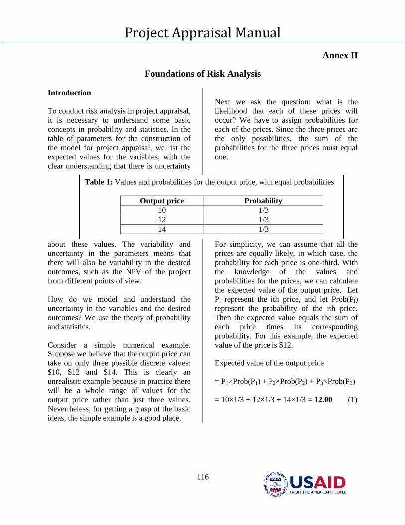
Project Appraisal Manual
116
Annex II
Foundations of Risk Analysis
Introduction
To conduct risk analysis in project appraisal,
it is necessary to understand some basic
concepts in probability and statistics. In the
table of parameters for the construction of
the model for project appraisal, we list the
expected values for the variables, with the
clear understanding that there is uncertainty
about these values. The variability and
uncertainty in the parameters means that
there will also be variability in the desired
outcomes, such as the NPV of the project
from different points of view.
How do we model and understand the
uncertainty in the variables and the desired
outcomes? We use the theory of probability
and statistics.
Consider a simple numerical example.
Suppose we believe that the output price can
take on only three possible discrete values:
$10, $12 and $14. This is clearly an
unrealistic example because in practice there
will be a whole range of values for the
output price rather than just three values.
Nevertheless, for getting a grasp of the basic
ideas, the simple example is a good place.
Next we ask the question: what is the
likelihood that each of these prices will
occur? We have to assign probabilities for
each of the prices. Since the three prices are
the only possibilities, the sum of the
probabilities for the three prices must equal
one.
For simplicity, we can assume that all the
prices are equally likely, in which case, the
probability for each price is one-third. With
the knowledge of the values and
probabilities for the prices, we can calculate
the expected value of the output price. Let
Pi represent the ith price, and let Prob(Pi)
represent the probability of the ith price.
Then the expected value equals the sum of
each price times its corresponding
probability. For this example, the expected
value of the price is $12.
Expected value of the output price
= P1×Prob(P1) + P2×Prob(P2) + P3×Prob(P3)
= 10×1/3 + 12×1/3 + 14×1/3 = 12.00 (1)
Table 1: Values and probabilities for the output price, with equal probabilities
Output price Probability
10 1/3
12 1/3
14 1/3
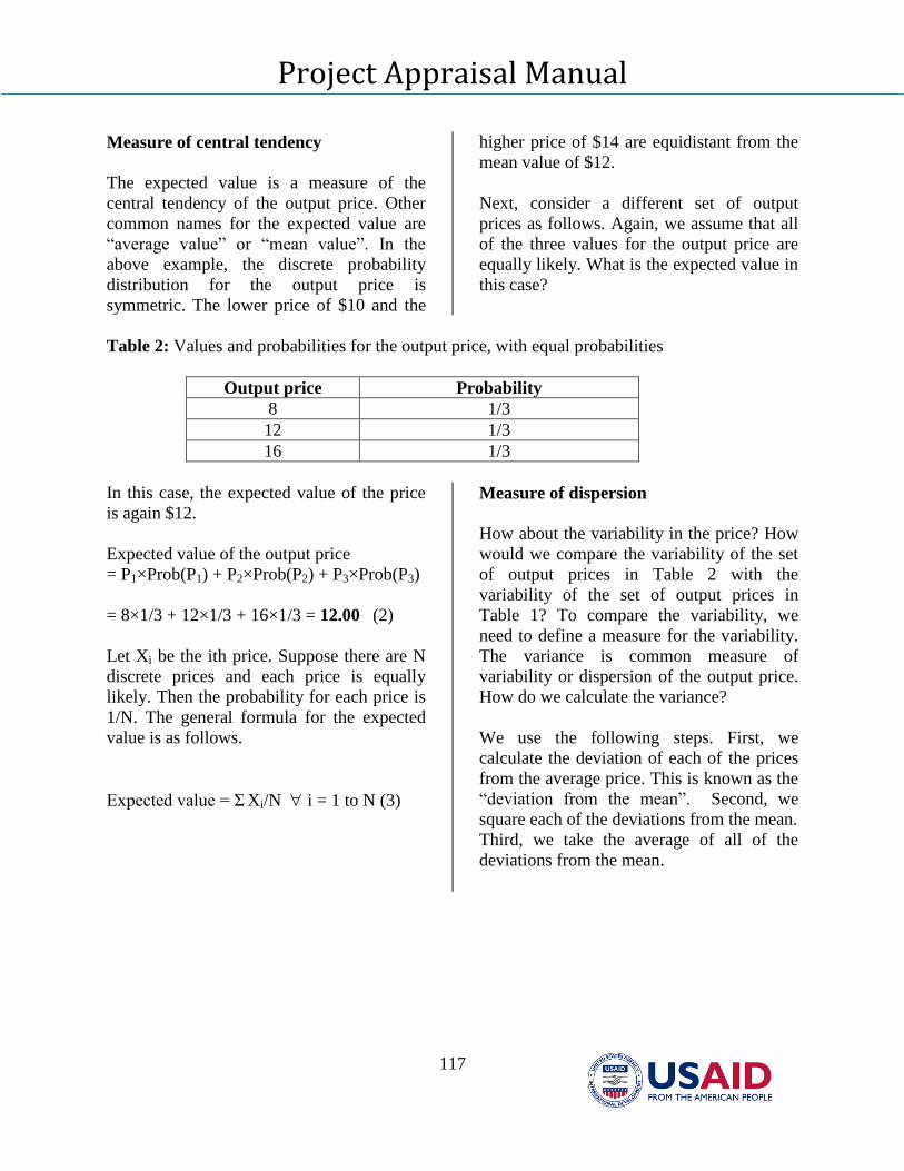
Project Appraisal Manual
117
Measure of central tendency
The expected value is a measure of the
central tendency of the output price. Other
common names for the expected value are
“average value” or “mean value”. In the
above example, the discrete probability
distribution for the output price is
symmetric. The lower price of $10 and the
higher price of $14 are equidistant from the
mean value of $12.
Next, consider a different set of output
prices as follows. Again, we assume that all
of the three values for the output price are
equally likely. What is the expected value in
this case?
Table 2: Values and probabilities for the output price, with equal probabilities
Output price Probability
8 1/3
12 1/3
16 1/3
In this case, the expected value of the price
is again $12.
Expected value of the output price
= P1×Prob(P1) + P2×Prob(P2) + P3×Prob(P3)
= 8×1/3 + 12×1/3 + 16×1/3 = 12.00 (2)
Let Xi be the ith price. Suppose there are N
discrete prices and each price is equally
likely. Then the probability for each price is
1/N. The general formula for the expected
value is as follows.
Expected value = Σ Xi/N i = 1 to N (3)
Measure of dispersion
How about the variability in the price? How
would we compare the variability of the set
of output prices in Table 2 with the
variability of the set of output prices in
Table 1? To compare the variability, we
need to define a measure for the variability.
The variance is common measure of
variability or dispersion of the output price.
How do we calculate the variance?
We use the following steps. First, we
calculate the deviation of each of the prices
from the average price. This is known as the
“deviation from the mean”. Second, we
square each of the deviations from the mean.
Third, we take the average of all of the
deviations from the mean.
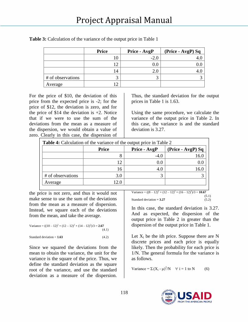
Project Appraisal Manual
118
Table 3: Calculation of the variance of the output price in Table 1
Price Price - AvgP (Price - AvgP) Sq
10 -2.0 4.0
12 0.0 0.0
14 2.0 4.0
# of observations 3 3 3
Average 12
For the price of $10, the deviation of this
price from the expected price is -2; for the
price of $12, the deviation is zero, and for
the price of $14 the deviation is +2. Notice
that if we were to use the sum of the
deviations from the mean as a measure of
the dispersion, we would obtain a value of
zero. Clearly in this case, the dispersion of
the price is not zero, and thus it would not
make sense to use the sum of the deviations
from the mean as a measure of dispersion.
Instead, we square each of the deviations
from the mean, and take the average.
Variance = ((10 – 12)2 + (12 – 12)2 + (14 – 12)2)/3 = 2.67
(4.1)
Standard deviation = 1.63 (4.2)
Since we squared the deviations from the
mean to obtain the variance, the unit for the
variance is the square of the price. Thus, we
define the standard deviation as the square
root of the variance, and use the standard
deviation as a measure of the dispersion.
Thus, the standard deviation for the output
prices in Table 1 is 1.63.
Using the same procedure, we calculate the
variance of the output price in Table 2. In
this case, the variance is and the standard
deviation is 3.27.
Variance = ((8 – 12)2 + (12 – 12)2 + (16 – 12)2)/3 = 10.67
(5.1) Standard deviation = 3.27 (5.2)
In this case, the standard deviation is 3.27.
And as expected, the dispersion of the
output price in Table 2 in greater than the
dispersion of the output price in Table 1.
Let Xi be the ith price. Suppose there are N
discrete prices and each price is equally
likely. Then the probability for each price is
1/N. The general formula for the variance is
as follows.
Variance = Σ (Xi - μ)2/N i = 1 to N (6)
Table 4: Calculation of the variance of the output price in Table 2
Price Price - AvgP (Price - AvgP) Sq
8 -4.0 16.0
12 0.0 0.0
16 4.0 16.0
# of observations 3.0 3 3
Average 12.0
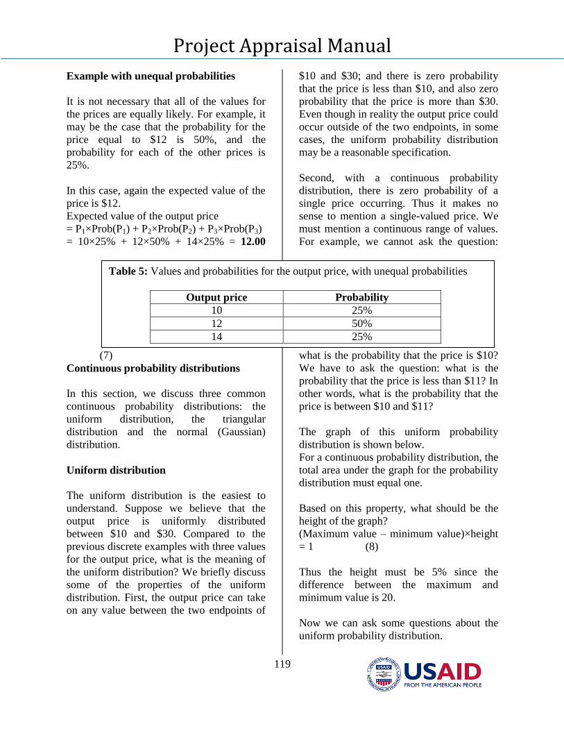
Project Appraisal Manual
119
Example with unequal probabilities
It is not necessary that all of the values for
the prices are equally likely. For example, it
may be the case that the probability for the
price equal to $12 is 50%, and the
probability for each of the other prices is
25%.
In this case, again the expected value of the
price is $12.
Expected value of the output price
= P1×Prob(P1) + P2×Prob(P2) + P3×Prob(P3)
= 10×25% + 12×50% + 14×25% = 12.00
(7)
Continuous probability distributions
In this section, we discuss three common
continuous probability distributions: the
uniform distribution, the triangular
distribution and the normal (Gaussian)
distribution.
Uniform distribution
The uniform distribution is the easiest to
understand. Suppose we believe that the
output price is uniformly distributed
between $10 and $30. Compared to the
previous discrete examples with three values
for the output price, what is the meaning of
the uniform distribution? We briefly discuss
some of the properties of the uniform
distribution. First, the output price can take
on any value between the two endpoints of
$10 and $30; and there is zero probability
that the price is less than $10, and also zero
probability that the price is more than $30.
Even though in reality the output price could
occur outside of the two endpoints, in some
cases, the uniform probability distribution
may be a reasonable specification.
Second, with a continuous probability
distribution, there is zero probability of a
single price occurring. Thus it makes no
sense to mention a single-valued price. We
must mention a continuous range of values.
For example, we cannot ask the question:
what is the probability that the price is $10?
We have to ask the question: what is the
probability that the price is less than $11? In
other words, what is the probability that the
price is between $10 and $11?
The graph of this uniform probability
distribution is shown below.
For a continuous probability distribution, the
total area under the graph for the probability
distribution must equal one.
Based on this property, what should be the
height of the graph?
(Maximum value – minimum value)×height
= 1 (8)
Thus the height must be 5% since the
difference between the maximum and
minimum value is 20.
Now we can ask some questions about the
uniform probability distribution.
Table 5: Values and probabilities for the output price, with unequal probabilities
Output price Probability
10 25%
12 50%
14 25%
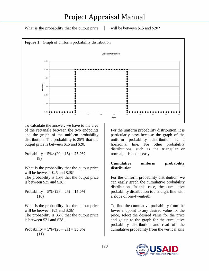
Project Appraisal Manual
120
What is the probability that the output price will be between $15 and $20?
Figure 1: Graph of uniform probability distribution
Uniform Distribution
0.0%
1.0%
2.0%
3.0%
4.0%
5.0%
6.0%
0 5 10 15 20 25 30 35 40 45 50
Price
Pro
bab
ilit
y
To calculate the answer, we have to the area
of the rectangle between the two endpoints
and the graph of the uniform probability
distribution. The probability is 25% that the
output price is between $15 and $20.
Probability = 5%×(20 – 15) = 25.0%
(9)
What is the probability that the output price
will be between $25 and $28?
The probability is 15% that the output price
is between $25 and $28.
Probability = 5%×(28 – 25) = 15.0%
(10)
What is the probability that the output price
will be between $21 and $28?
The probability is 35% that the output price
is between $21 and $28.
Probability = 5%×(28 – 21) = 35.0%
(11)
For the uniform probability distribution, it is
particularly easy because the graph of the
uniform probability distribution is a
horizontal line. For other probability
distributions, such as the triangular or
normal, it is not as easy.
Cumulative uniform probability
distribution
For the uniform probability distribution, we
can easily graph the cumulative probability
distribution. In this case, the cumulative
probability distribution is a straight line with
a slope of one-twentieth.
To find the cumulative probability from the
lower endpoint to any desired value for the
price, select the desired value for the price
and go up to the graph for the cumulative
probability distribution and read off the
cumulative probability from the vertical axis
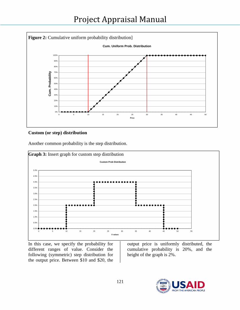
Project Appraisal Manual
121
Figure 2: Cumulative uniform probability distribution]
Cum. Uniform Prob. Distribution
0%
10%
20%
30%
40%
50%
60%
70%
80%
90%
100%
0 5 10 15 20 25 30 35 40 45 50
Price
Cu
m.
Pro
bab
ilit
y
Custom (or step) distribution
Another common probability is the step distribution.
Graph 3: Insert graph for custom step distribution
Custom Prob Distribution
0.0%
0.5%
1.0%
1.5%
2.0%
2.5%
3.0%
3.5%
4.0%
4.5%
5.0%
0 5 10 15 20 25 30 35 40 45 50 55
X values
In this case, we specify the probability for
different ranges of value. Consider the
following (symmetric) step distribution for
the output price. Between $10 and $20, the
output price is uniformly distributed, the
cumulative probability is 20%, and the
height of the graph is 2%.
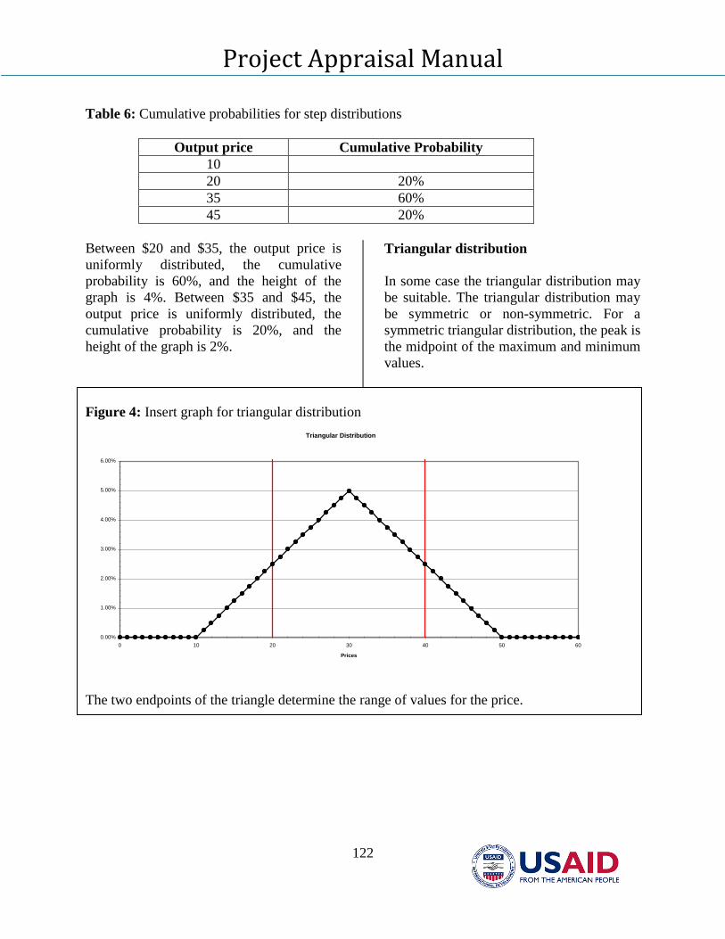
Project Appraisal Manual
122
Table 6: Cumulative probabilities for step distributions
Output price Cumulative Probability
10
20 20%
35 60%
45 20%
Between $20 and $35, the output price is
uniformly distributed, the cumulative
probability is 60%, and the height of the
graph is 4%. Between $35 and $45, the
output price is uniformly distributed, the
cumulative probability is 20%, and the
height of the graph is 2%.
Triangular distribution
In some case the triangular distribution may
be suitable. The triangular distribution may
be symmetric or non-symmetric. For a
symmetric triangular distribution, the peak is
the midpoint of the maximum and minimum
values.
Figure 4: Insert graph for triangular distribution
Triangular Distribution
0.00%
1.00%
2.00%
3.00%
4.00%
5.00%
6.00%
0 10 20 30 40 50 60
Prices
The two endpoints of the triangle determine the range of values for the price.
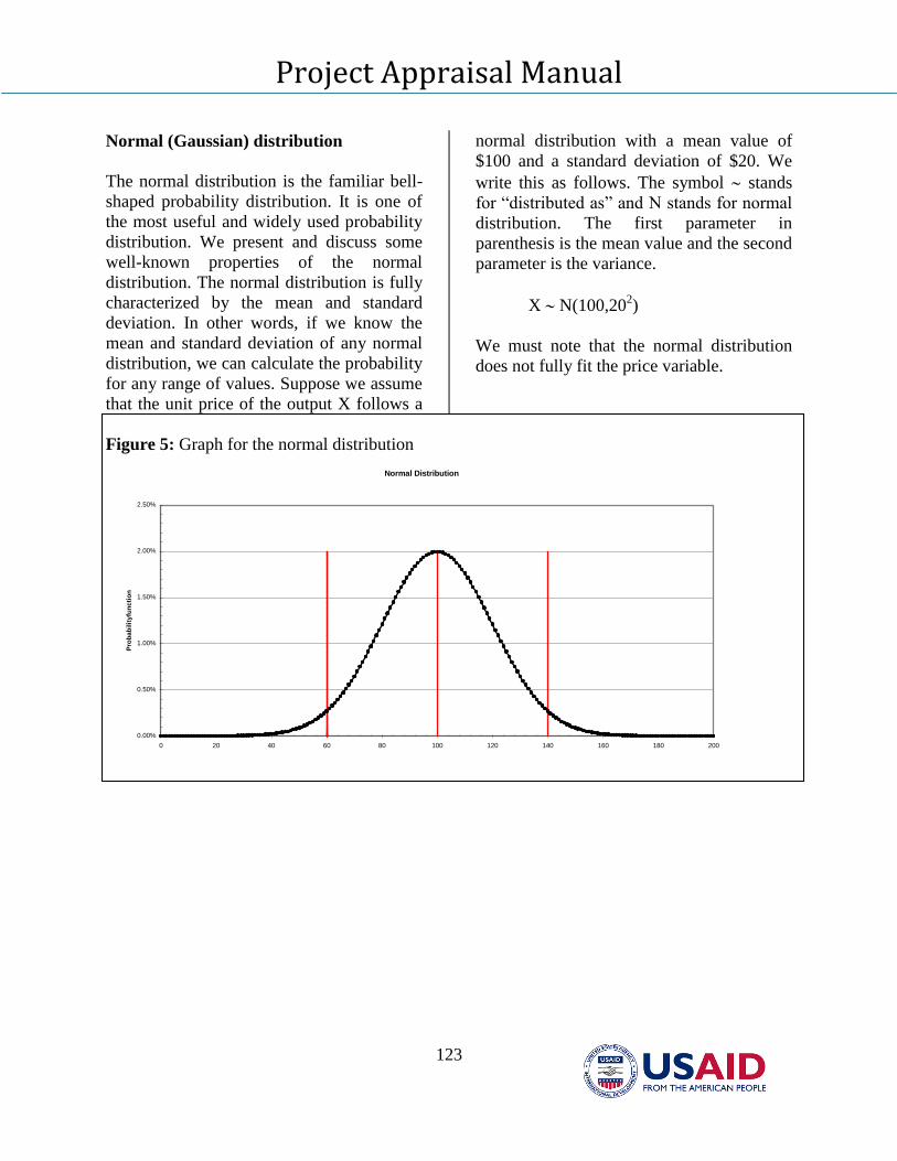
Project Appraisal Manual
123
Normal (Gaussian) distribution
The normal distribution is the familiar bell-
shaped probability distribution. It is one of
the most useful and widely used probability
distribution. We present and discuss some
well-known properties of the normal
distribution. The normal distribution is fully
characterized by the mean and standard
deviation. In other words, if we know the
mean and standard deviation of any normal
distribution, we can calculate the probability
for any range of values. Suppose we assume
that the unit price of the output X follows a
normal distribution with a mean value of
$100 and a standard deviation of $20. We
write this as follows. The symbol stands
for “distributed as” and N stands for normal
distribution. The first parameter in
parenthesis is the mean value and the second
parameter is the variance.
X N(100,202)
We must note that the normal distribution
does not fully fit the price variable.
Figure 5: Graph for the normal distribution
Normal Distribution
0.00%
0.50%
1.00%
1.50%
2.00%
2.50%
0 20 40 60 80 100 120 140 160 180 200
Pro
bab
ilit
yfu
ncti
on
Project Appraisal Manual
124
For example, the normal distribution ranges
from minus infinity to plus infinity. Clearly,
the price cannot take negative values and
there is some upper limit to the price.
Nevertheless, for practical purposes, the
normal distribution is convenient to use and
appropriate.
With the normal distribution there are some
well-known rules about the probability
between given ranges of values.
Rule One Sigma
We can ask the question: what is the
probability that the output price is within
one standard deviation of the mean? In other
words, what is the probability that the price
X is between 80, which is one standard
deviation (or one sigma) below the mean
and 120, which is one standard deviation
above the mean? The answer, for any
normal distribution, is 68%.
Prob (μ – σ ≤ X ≤ μ + σ) = Prob (100 - 20 ≤
X ≤ 100 + 20)
= Prob (80 ≤ X ≤ 120) = 68% (12)
Rule Two Sigma
What about the probability that the price is
within two standard deviations of the mean?
In other words, what is the probability that
the price is between 60, which is two
standard deviations (or two sigmas) below
the mean and 120, which is two standard
deviations above the mean? The answer, for
any normal distribution, is 95%.
Prob (μ – 2σ ≤ X ≤ μ + 2σ) = Prob (100 -
2×20 ≤ X ≤ 100 + 2×20)
= Prob (60 ≤ X ≤ 140) = 95% (13)
Rule Three Sigma
What about the probability that the price is
within three standard deviations of the
mean? For any normal distribution, the
probability is 99% that the price is within
three standard deviations of the mean.
Prob (μ – 3σ ≤ X ≤ μ + 3σ) = Prob (100 -
3×20 ≤ X ≤ 100 + 3×20)
= Prob (40 ≤ X ≤ 160) = 99%
(14)
Based on these three rules about one, two
and three sigma, we can answer the
following additional questions for a normal
distribution.
What is the probability that the output price
X is above $120? In other words, what is the
probability that the output price X is one
standard deviation above the mean?
Prob (X ≥ μ + σ) = Prob (X ≥ 100 + 20)
= Prob (X ≥ 120) = ?
From the rule one sigma, we know the
following.
Prob (μ – σ ≤ X ≤ μ + σ) = Prob (100 - 20 ≤
X ≤ 100 + 20)
= Prob (80 ≤ X ≤ 120) = 68%
(15)
The probability that the output price is more
than 2 standard deviations from the mean (in
absolute value terms) is 32%. In other
words, the combined probability that X is
either one standard deviation below the
mean or one standard deviation above the
mean is 32%.
Prob (X ≤ μ – σ) or Prob (X ≥ μ + σ) =
100% - 68% = 32.0%(16)
Since the normal probability distribution is
symmetric, it means that the probability of
the lower tail equals the probability of the
Project Appraisal Manual
125
upper tail of the probability distribution.
Thus, the probability that the output price is
one standard deviation above the mean is
16%.
Prob (X ≥ 120) = 32%/2 =16.0%
(17)
What is the probability that the output price
X is below $140? In other words, what is the
probability that the output price X is two
standard deviations below the mean?
Prob (X ≤ μ - 2σ) = Prob (X ≤ 100 - 40) =
Prob (X ≤ 60) = ?
From the rule two sigma, we know the
following.
Prob (μ – 2σ ≤ X ≤ μ + 2σ) = Prob (100 -
2×20 ≤ X ≤ 100 + 2×20)
= Prob (60 ≤ X ≤ 140) = 95%
(18)
The probability that the output price is more
than 2 standard deviations from the mean (in
absolute value terms) is 95%. In other
words, the combined probability that X is
either two standard deviations below the
mean or two standard deviations above the
mean is 5%.
Prob (X ≤ μ – 2σ) or Prob (X ≥ μ + 2σ) =
100% - 95% = 5.0%(19)
Since the normal probability distribution is
symmetric, it means that the probability of
the lower tail equals the probability of the
upper tail of the probability distribution.
Thus, the probability that the output price is
one standard deviation above the mean is
2.5%.
Prob (X ≤ 60) = 5%/2 = 2.5%
(20)
What is the probability that the output price
X is between $80 and $140? In other words,
what is the probability that the output price
X is between one standard deviation below
the mean and two standard deviations above
the mean?
Prob (μ – σ ≤ X ≤ μ + 2σ) = Prob (100 - 20
≤ X ≤ 100 + 2×20)
= Prob (80 ≤ X ≤ 140) = ?
To answer this question, we can rewrite it as
the sum of two probabilities, namely the
probability between one standard deviation
below the mean and the mean plus the
probability between the mean and two
standard deviations above the mean.
Prob (μ – σ ≤ X ≤ μ + 2σ) = Prob (μ – σ ≤ X
≤ μ)
+ Prob (μ ≤ X ≤ μ + 2σ)
= Prob (80 ≤ X ≤ 100)
+ Prob (100 ≤ X ≤ 140)
(21)
The probability between one standard
deviation below the mean and the mean is
34%.
Prob (μ – σ ≤ X ≤ μ) = Prob (80 ≤ X ≤ 100)
= 34% (22)
The probability between the mean and two
standard deviations above the mean is 2.5%.
Prob (μ ≤ X ≤ μ + 2σ) = Prob (100 ≤ X ≤
140) = 50% - 2.5%
= 47.5%
(23)
Thus, the combined probability is 81.5%.
Prob (μ – σ ≤ X ≤ μ + 2σ) = 34% + 47.5% =
81.5% (24)
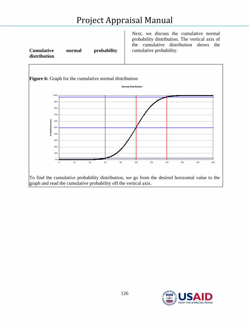
Project Appraisal Manual
126
Cumulative normal probability
distribution
Next, we discuss the cumulative normal
probability distribution. The vertical axis of
the cumulative distribution shows the
cumulative probability.
Figure 6: Graph for the cumulative normal distribution
Normal Distribution
0%
10%
20%
30%
40%
50%
60%
70%
80%
90%
100%
0 20 40 60 80 100 120 140 160 180 200
Pro
bab
ilit
yfu
ncti
on
To find the cumulative probability distribution, we go from the desired horizontal value to the
graph and read the cumulative probability off the vertical axis.
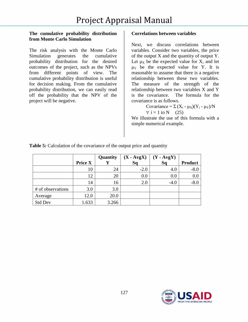
Project Appraisal Manual
127
The cumulative probability distribution
from Monte Carlo Simulation
The risk analysis with the Monte Carlo
Simulation generates the cumulative
probability distribution for the desired
outcomes of the project, such as the NPVs
from different points of view. The
cumulative probability distribution is useful
for decision making. From the cumulative
probability distribution, we can easily read
off the probability that the NPV of the
project will be negative.
Correlations between variables
Next, we discuss correlations between
variables. Consider two variables, the price
of the output X and the quantity of output Y.
Let μX be the expected value for X, and let
μY be the expected value for Y. It is
reasonable to assume that there is a negative
relationship between these two variables.
The measure of the strength of the
relationship between two variables X and Y
is the covariance. The formula for the
covariance is as follows.
Covariance = Σ (Xi - μX)(Yi - μY)/N
i = 1 to N (25)
We illustrate the use of this formula with a
simple numerical example.
Table 5: Calculation of the covariance of the output price and quantity
Price X
Quantity
Y
(X - AvgX)
Sq
(Y - AvgY)
Sq Product
10 24 -2.0 4.0 -8.0
12 20 0.0 0.0 0.0
14 16 2.0 -4.0 -8.0
# of observations 3.0 3.0
Average 12.0 20.0
Std Dev 1.633 3.266
Project Appraisal Manual
128
First, we calculate the deviation of the X
values from the expected X value, and the
deviation of the Y values from the expected
Y value. Second, we multiply the deviation
of the ith X value and the corresponding
deviation for the ith Y value. Third, we take
the average.
Covariance = (-2×4 + 0×0 + 2×-4)/3 = -2.67
(26)
We cannot use the covariance measure to
compare the strength of the relationships
between pairs of variables because the units
for the covariance are the product of the
units for the two variables.
We define the correlation coefficient as
follows. The correlation coefficient equals
the covariance divided by the product of the
standard deviation of X and the standard
deviation of Y.
Correl(X,Y) = Covariance(X,Y)/(σX×σY)
= -2.67 /(1.633×3.266) = -0.50(27)
In this case, the correlation coefficient
between X and Y is -0.50. By definition, if
the two variables are perfectly positively
correlated, the maximum value for the
correlation coefficient is +1; if the two
variables are perfectly negatively correlated,
the minimum value for the correlation
coefficient is -1.
If the two variables are perfectly positively
correlated, it means that the values of X
equal the values of Y. The formula for the
covariance in the numerator is identical to
the formula for the variance, and the product
in the denominator also equals the variance.
Thus the maximum possible value is +1. If
the two variables are perfectly negatively
correlated, it means that the values of X
equal the negative of the values of Y. And
thus, the minimum possible value is -1.
Project Appraisal Manual
129
Annex III
Principles of Risk Analysis and Management
In this section, we present the principles of
risk analysis and management. Risk analysis
and management are integral components of
the project appraisal framework. In the
previous discussion on the construction of
the financial and economic cash flow
statements, we postponed the issue of
uncertainty and simply specified the
expected values for the key variables in the
table of parameters. Based on these expected
values, in the subsequent tables of the
project appraisal, we entered formulas that
were linked to the key variables in the table
of parameters. It is extremely important that
the formulas are properly linked. If the
formulas for the desired outcomes, such as
the NPVs from the different points of view,
are not properly linked, then it would not be
possible to conduct risk analysis.
In the risk analysis, we introduce uncertainty
explicitly into the project appraisal and
analyze the risk profiles of the nominal cash
flows from different points of view. After
we have a good understanding of the risk
profiles of the cash flows from different
points of view, we move forward and
examine the issue of risk diversification and
management. The risk analysis enables us to
identify and focus on the key variables on
which we may wish to acquire better
information.
In the risk analysis, first, we identify,
analyze and interpret the expected
variability in the desired project outcomes
from alternative points of view. We discuss
sensitivity analysis, scenario analysis and
Monte Carlo Simulation (MCS).
Second, we discuss the sources of risk and
the issue of risk diversification, using some
simple variance relationships.
Third, we examine how we can redesign and
reorganize the project to allocate, and if
necessary reallocate, the risk in a more
efficient manner.
Risk analysis
The motivation and necessity for risk
analysis is straight-forward. As mentioned
earlier, there is uncertainty in the values of
the key variables that we list in the table of
parameters for the project appraisal. The
variability in the key variables affects the
desired outcomes, such as the Net Present
Value (NPV) of the project from different
points of view. Thus we have to examine
how changes in the values of the key
variables impact the desired outcomes. With
the results of this analysis, we can examine
issues in risk management and the design of
contracts for risk allocation.
Since the nominal cash flow profiles for a
project extend over many years, there is
uncertainty both at a given point in time and
across time. For example, in a given year,
there may be variability in the unit price of
the output. Also, we recognize that the unit
price of the output may change over time, in
which case we have to model the
correlations, if any, between prices over
time.
There are alternative methods for risk
analysis, ranging from the simple to the
complex.
1. Sensitivity analysis
Project Appraisal Manual
130
2. Scenario analysis
3. Monte Carlo Simulation (MCS)
Below, we describe each of the three
methods.
Sensitivity analysis
In the table of parameters for a project
appraisal, we list the expected values for the
key variables, with the recognition that there
is uncertainty about the values for the
variables. In the sensitivity analysis, we
examine how changes in the values of one of
these variables, holding constant the values
of all of the variables, affect the NPV of the
net cash flow. Sensitivity analysis is also
known as “what-if” analysis.
In EXCEL, it is easy to create simple one-
way and two-way tables (sensitivity tables)
that show how changes in the value of a
certain variable impact on the NPV of the
project, ceteris paribus (holding constant the
values of all the other variables). The
generation of the one-way tables requires
that the cells for the desired outcomes are
properly linked to the variables in the table
of parameters. It is very important to keep in
mind the ceteris paribus condition. As we
discuss later, we must recognize that in
reality many variables are changing
simultaneously.
Also, with sensitivity analysis, we can
conduct break-even analysis for each of the
key variables. For example, we can
determine the output price that will cause
the NPV of the project to switch from
positive to negative. The break-even values
for each of the key variables will provide a
qualitative assessment of the extent to which
the project is responsive to changes in the
values of the key variables.
Furthermore, sensitivity analysis is a
powerful diagnostic tool for assessing the
construction of the overall financial models.
For many variables, we know the direction
of the impact of changes in the value of the
variable on the desired outcomes. For
example, generally speaking, an increase in
the expected inflation rate should have a
negative impact on the NPV of the project,
taking into account all the direct and indirect
effects of inflation. If the sensitivity analysis
reveals that an increase in the expected
inflation rate leads to an increase in the NPV
of the project, it is most likely that there is
an error in the modeling. If there is no error,
then the analyst should be able to identify
the reason(s) why inflation is creating value.
We illustrate the ideas and concepts of
sensitivity analysis with the following
simple numerical example. Suppose a
project sells 10 units each year, and at the
end of year 0, the unit price is Iraqi Dinars.
20, which increases at the expected inflation
rate of 5%. The real discount rate is 10%,
and with an expected inflation rate of 5%,
the nominal discount rate is 15.5%.
First we construct the inflation index, and
obtain the nominal price profile by
multiplying the initial unit price in year 0
with the expected inflation index.
Table 1: Inflation index and nominal price profile
Year 0 1 2 3 4 5
Inflation index 1.000 1.050 1.103 1.158 1.216 1.276
Nominal unit
price 21.00 22.05 23.15 24.31 25.53
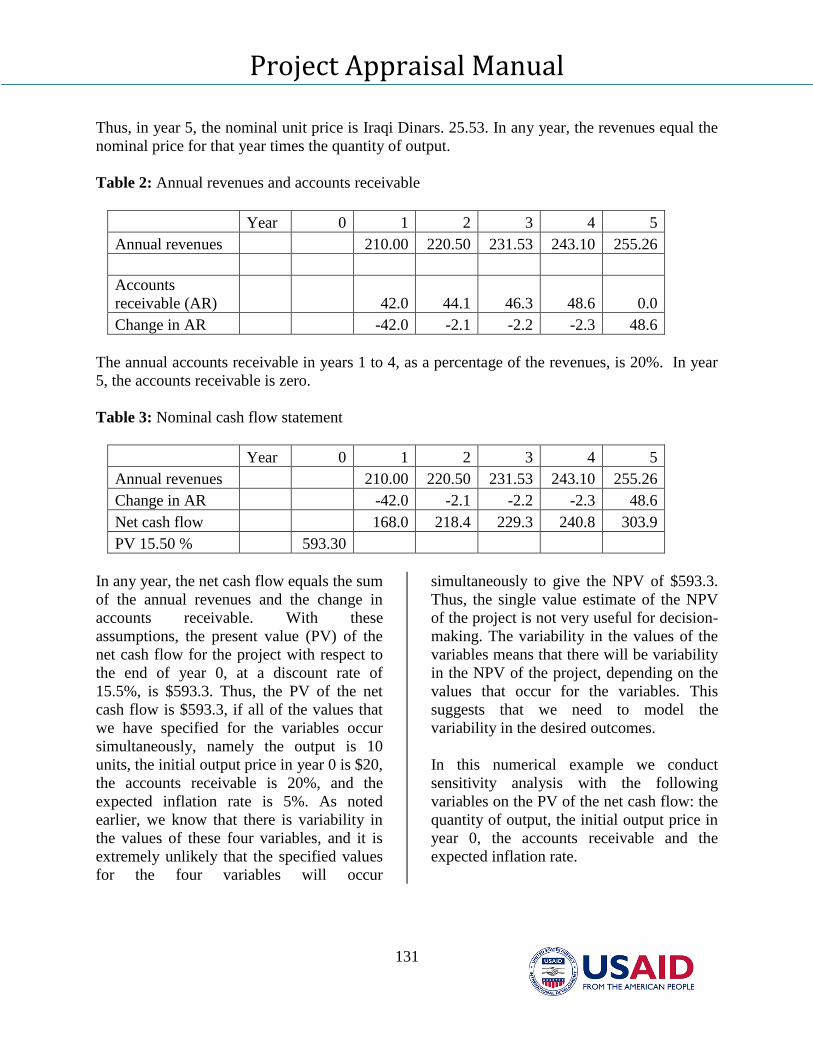
Project Appraisal Manual
131
Thus, in year 5, the nominal unit price is Iraqi Dinars. 25.53. In any year, the revenues equal the
nominal price for that year times the quantity of output.
Table 2: Annual revenues and accounts receivable
Year 0 1 2 3 4 5
Annual revenues 210.00 220.50 231.53 243.10 255.26
Accounts
receivable (AR) 42.0 44.1 46.3 48.6 0.0
Change in AR -42.0 -2.1 -2.2 -2.3 48.6
The annual accounts receivable in years 1 to 4, as a percentage of the revenues, is 20%. In year
5, the accounts receivable is zero.
Table 3: Nominal cash flow statement
Year 0 1 2 3 4 5
Annual revenues 210.00 220.50 231.53 243.10 255.26
Change in AR -42.0 -2.1 -2.2 -2.3 48.6
Net cash flow 168.0 218.4 229.3 240.8 303.9
PV 15.50 % 593.30
In any year, the net cash flow equals the sum
of the annual revenues and the change in
accounts receivable. With these
assumptions, the present value (PV) of the
net cash flow for the project with respect to
the end of year 0, at a discount rate of
15.5%, is $593.3. Thus, the PV of the net
cash flow is $593.3, if all of the values that
we have specified for the variables occur
simultaneously, namely the output is 10
units, the initial output price in year 0 is $20,
the accounts receivable is 20%, and the
expected inflation rate is 5%. As noted
earlier, we know that there is variability in
the values of these four variables, and it is
extremely unlikely that the specified values
for the four variables will occur
simultaneously to give the NPV of $593.3.
Thus, the single value estimate of the NPV
of the project is not very useful for decision-
making. The variability in the values of the
variables means that there will be variability
in the NPV of the project, depending on the
values that occur for the variables. This
suggests that we need to model the
variability in the desired outcomes.
In this numerical example we conduct
sensitivity analysis with the following
variables on the PV of the net cash flow: the
quantity of output, the initial output price in
year 0, the accounts receivable and the
expected inflation rate.
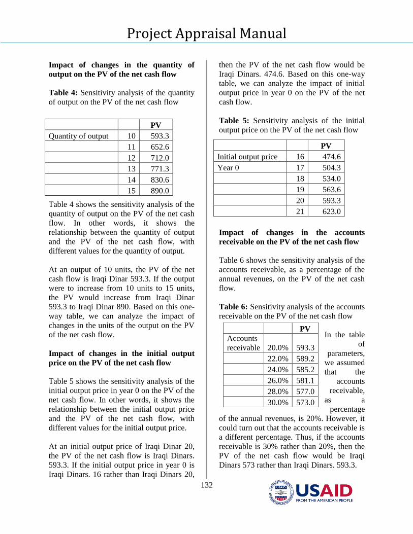
Project Appraisal Manual
132
Impact of changes in the quantity of
output on the PV of the net cash flow
Table 4: Sensitivity analysis of the quantity
of output on the PV of the net cash flow
Table 4 shows the sensitivity analysis of the
quantity of output on the PV of the net cash
flow. In other words, it shows the
relationship between the quantity of output
and the PV of the net cash flow, with
different values for the quantity of output.
At an output of 10 units, the PV of the net
cash flow is Iraqi Dinar 593.3. If the output
were to increase from 10 units to 15 units,
the PV would increase from Iraqi Dinar
593.3 to Iraqi Dinar 890. Based on this one-
way table, we can analyze the impact of
changes in the units of the output on the PV
of the net cash flow.
Impact of changes in the initial output
price on the PV of the net cash flow
Table 5 shows the sensitivity analysis of the
initial output price in year 0 on the PV of the
net cash flow. In other words, it shows the
relationship between the initial output price
and the PV of the net cash flow, with
different values for the initial output price.
At an initial output price of Iraqi Dinar 20,
the PV of the net cash flow is Iraqi Dinars.
593.3. If the initial output price in year 0 is
Iraqi Dinars. 16 rather than Iraqi Dinars 20,
then the PV of the net cash flow would be
Iraqi Dinars. 474.6. Based on this one-way
table, we can analyze the impact of initial
output price in year 0 on the PV of the net
cash flow.
Table 5: Sensitivity analysis of the initial
output price on the PV of the net cash flow
Impact of changes in the accounts
receivable on the PV of the net cash flow
Table 6 shows the sensitivity analysis of the
accounts receivable, as a percentage of the
annual revenues, on the PV of the net cash
flow.
Table 6: Sensitivity analysis of the accounts
receivable on the PV of the net cash flow
In the table
of
parameters,
we assumed
that the
accounts
receivable,
as a
percentage
of the annual revenues, is 20%. However, it
could turn out that the accounts receivable is
a different percentage. Thus, if the accounts
receivable is 30% rather than 20%, then the
PV of the net cash flow would be Iraqi
Dinars 573 rather than Iraqi Dinars. 593.3.
PV
Quantity of output 10 593.3
11 652.6
12 712.0
13 771.3
14 830.6
15 890.0
PV
Initial output price 16 474.6
Year 0 17 504.3
18 534.0
19 563.6
20 593.3
21 623.0
PV
Accounts
receivable 20.0% 593.3
22.0% 589.2
24.0% 585.2
26.0% 581.1
28.0% 577.0
30.0% 573.0
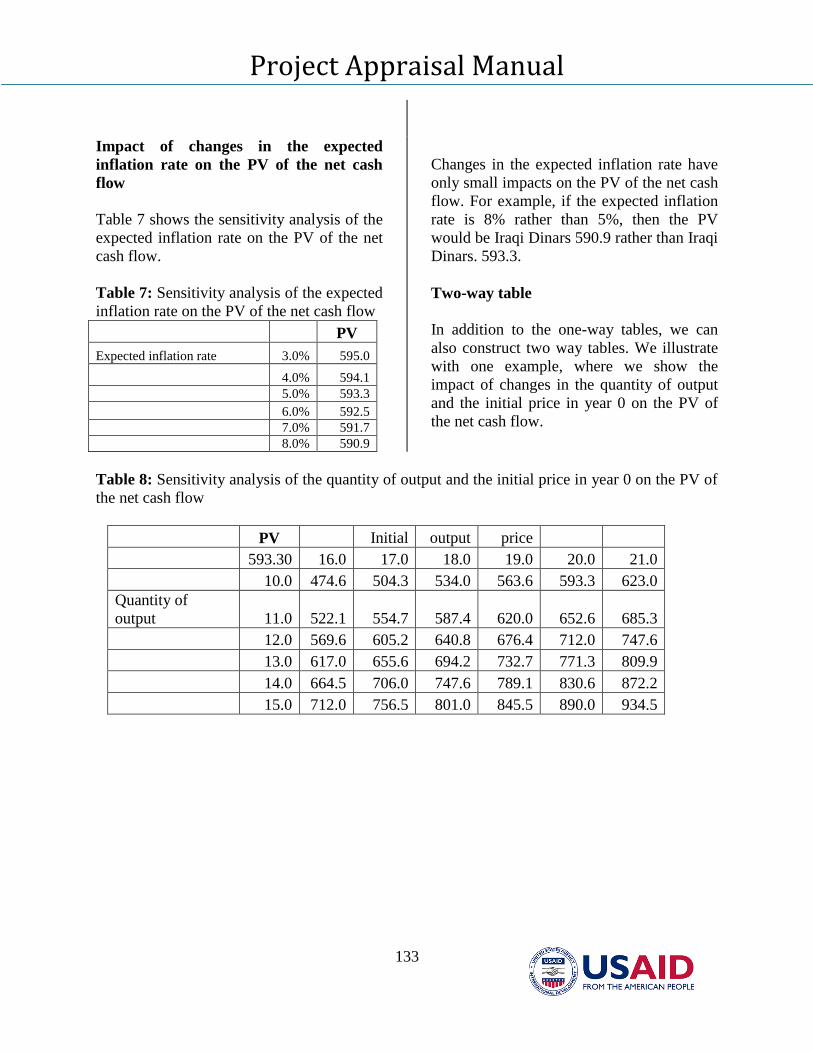
Project Appraisal Manual
133
Impact of changes in the expected
inflation rate on the PV of the net cash
flow
Table 7 shows the sensitivity analysis of the
expected inflation rate on the PV of the net
cash flow.
Table 7: Sensitivity analysis of the expected
inflation rate on the PV of the net cash flow
PV
Expected inflation rate 3.0% 595.0
4.0% 594.1
5.0% 593.3
6.0% 592.5
7.0% 591.7
8.0% 590.9
Changes in the expected inflation rate have
only small impacts on the PV of the net cash
flow. For example, if the expected inflation
rate is 8% rather than 5%, then the PV
would be Iraqi Dinars 590.9 rather than Iraqi
Dinars. 593.3.
Two-way table
In addition to the one-way tables, we can
also construct two way tables. We illustrate
with one example, where we show the
impact of changes in the quantity of output
and the initial price in year 0 on the PV of
the net cash flow.
Table 8: Sensitivity analysis of the quantity of output and the initial price in year 0 on the PV of
the net cash flow
PV Initial output price
593.30 16.0 17.0 18.0 19.0 20.0 21.0
10.0 474.6 504.3 534.0 563.6 593.3 623.0
Quantity of
output 11.0 522.1 554.7 587.4 620.0 652.6 685.3
12.0 569.6 605.2 640.8 676.4 712.0 747.6
13.0 617.0 655.6 694.2 732.7 771.3 809.9
14.0 664.5 706.0 747.6 789.1 830.6 872.2
15.0 712.0 756.5 801.0 845.5 890.0 934.5
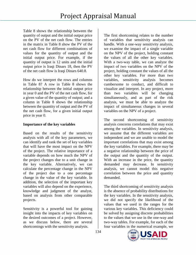
Project Appraisal Manual
134
Table 8 shows the relationship between the
quantity of output and the initial output price
on the PV of the net cash flow. The entries
in the matrix in Table 8 show the PV of the
net cash flow for different combinations of
values for the quantity of output and the
initial output price. For example, if the
quantity of output is 12 units and the initial
output price is Iraqi Dinars 18, then the PV
of the net cash flow is Iraqi Dinars 640.8.
How do we interpret the rows and columns
in Table 8? A row in Table 8 shows the
relationship between the initial output price
in year 0 and the PV of the net cash flow, for
a given value of the quantity of output; and a
column in Table 8 shows the relationship
between the quantity of output and the PV of
the net cash flow, for a given initial output
price in year 0.
Importance of the key variables
Based on the results of the sensitivity
analysis with all of the key parameters, we
can identify and rank the set of key variables
that will have the most impact on the NPV
of the project. The relative importance of a
variable depends on how much the NPV of
the project changes due to a unit change in
the key variable. Alternatively, we can
calculate the percentage change in the NPV
of the project due to a one percentage
change in the value of the key variable. In
addition, the selection of the important key
variables will also depend on the experience,
knowledge and judgment of the analyst,
based on analysis from other comparable
projects.
Sensitivity is a powerful tool for gaining
insight into the impacts of key variables on
the desired outcomes of a project. However,
as we discuss below, there are several
shortcomings with the sensitivity analysis.
The first shortcoming relates to the number
of variables that sensitivity analysis can
handle. With a one-way sensitivity analysis,
we examine the impact of a single variable
on the NPV of the project, holding constant
the values of all the other key variables.
With a two-way table, we can analyze the
impact of two variables on the NPV of the
project, holding constant the values of all the
other key variables. For more than two
variables, sensitivity analysis becomes
cumbersome to conduct, and difficult to
visualize and interpret. In any project, more
than two variables will be changing
simultaneously, and as part of the risk
analysis, we must be able to analyze the
impact of simultaneous changes in several
variables on the NPV of a project.
The second shortcoming of sensitivity
analysis concerns correlations that may exist
among the variables. In sensitivity analysis,
we assume that the different variables are
independent and we are unable to model the
important correlations that may exist among
the key variables. For example, there may be
a negative relationship between the price of
the output and the quantity of the output.
With an increase in the price, the quantity
demanded may decrease. In sensitivity
analysis, we cannot model this negative
correlation between the price and quantity
demanded.
The third shortcoming of sensitivity analysis
is the absence of probability distributions for
the key variables. In the sensitivity analysis,
we did not specify the likelihood of the
values that we used in the ranges for the
various key variables. This deficiency could
be solved by assigning discrete probabilities
to the values that we use in the one-way and
two-way tables. For example, for each of the
four variables in the numerical example, we
Project Appraisal Manual
135
could assign discrete probabilities
distributions for the range of values.
However, with multiple variables, it would
be quite tedious to implement, and
furthermore, the interpretation of the results
would also be problematic.
As we shall see below, the use of Monte
Carlo Simulation (MCS) is the natural way
to overcome the shortcomings of the
sensitivity analysis. Before discussing MCS,
we briefly discuss an intermediate method,
which is scenario analysis.
Scenario analysis
Scenario analysis is a partial remedy for the
shortcomings of sensitivity analysis. Based
on the set of key variables that have been
identified through the sensitivity analysis,
we describe three scenarios: best case (or
optimistic case), expected case, and worst
case (pessimistic case). Each scenario is
based on a combination of possible values
from the set of key variables. The analyst is
not restricted to three scenarios, and could
specify five or more scenarios. How many
variables should we use in the specification
of the scenarios? Four or five variables
should be sufficient for practical purposes.
With more variables, the construction and
interpretation of the scenarios will be
difficult.
How do we use the results of the scenario
analysis? Under two extreme cases, we may
decide as follows. If the NPV of the project
is negative in the best case scenario, then it
is reasonable to reject the project.
Alternatively, if the NPV of the project is
positive in the worst case scenario, then we
should accept the project. In practice, the
results may not be so clear cut.
Scenario analysis also suffers from the other
shortcomings that we had identified
previously in sensitivity analysis. We are
unable to assess the likelihood of the
different scenarios because the scenario
analysis does not specify the probabilities
for the values of the different variables that
form the basis for the scenarios.
Furthermore, we cannot specify the
correlations that may exist among the
variables.
Monte Carlo Simulation
Of the three methods mentioned above,
Monte Carlo Simulation (MCS) is the most
complicated method for risk analysis. MCS
is a natural extension of sensitivity analysis
and overcomes the two major shortcomings
of sensitivity analysis. As a result, it also
increases the level of complexity in the
analysis. However, with the development of
easy-to-use software, it is relatively simple
to conduct sophisticated Monte Carlo
Simulations for project appraisal.
With MCS, we can specify probability
distributions for the key risk variables,
specify correlations that exist among the risk
variables, and can model a reasonably large
number of variables in a sensible manner.
By specifying the probability distributions
for the variables, we obtain the probability
distributions for any desired outcomes, such
as the NPV of the project from different
points of view.
In conducting a MCS, we undertake
the following steps.
1. Mathematical model: project
appraisal spreadsheet,
2. Identify variables that are sensitive
and uncertain,
3. Define uncertainty
a. Specify probability
distributions
Project Appraisal Manual
136
4. Identify and define correlated
variables
a. Positive or negative
correlation
b. Strength of correlation
5. Run the simulation model
6. Analysis of results
a. Summary statistics
b. Probability distributions of
desired outcomes
Next we briefly comment on each of the
steps for the MCS. In the first step we
construct the mathematical model for the
project appraisal. As mentioned earlier, we
have to ensure that the desired outcomes,
such as the NPV of the project from
different points of view, are properly linked
via formulas to all of the previous tables and
to the key variables in the table of
parameters. Without such proper linkages,
we will not be able to conduct sensitivity
analysis and the MCS.
In the second step, we conduct sensitivity
analysis with one-way and two-way tables to
identify the key risk variables. From a
practical point of view, six to eight risk
variables would be a reasonable number. If
the project is particularly complex, then a
larger number of risk variables may be
justified. However, a complicated analysis
with a lot of risk variables may not
necessarily lead to greater insight about the
risk of the project.
In the third step, we specify the probability
distributions for the risk variables.
Commonly used distributions are: the
uniform, triangular and normal. If there is
historical information or data on the risk
variables, then we can use the historical
information to guide us in the specification
of the probability distributions. If there is no
historical data, then we may have to rely on
the opinions of experts or practitioners who
may have good judgment on the likely range
for the future movement of the values of the
risk variables. Also, we may look for
secondary data from the published literature
and data for variables from other
comparable and similar projects.
In the fourth step, we specify the direction
(positive or negative) and strength of the
correlations that may exist among the risk
variables.
In the fifth step, we run the simulation
model, and obtain the simulation results.
The simulation results consist of summary
statistics and probability distributions for all
the variables and outcomes.
Interpretation of the simulation results
The most useful graphs are the cumulative
probability distribution graphs for the NPV
from different points of view. From the
cumulative probability graph, the decision
maker can easily determine the probability
that the NPV of the project is positive.
For more details on the probability and
statistical concepts that are relevant for risk
analysis, please see the section on the
foundations of risk analysis.

Project Appraisal Manual
137
Chapter VIII: Risk Management
Project Appraisal Manual
138
CHAPTER VIII: RISK MANAGEMENT
Next, we discuss risk management. In risk
management, we examine different ways to
structure the internal and external
relationships in a project. We can use
contracts and other arrangements to improve
the incentives that the different stakeholders
face.
Before discussing risk management, we
briefly describe the sources of risk in a
project.
Sources of risk in a project
What are the sources of risk in a project?
The risks that affect a project can be external
(or exogenous) or internal (endogenous).
First, we consider different types of external
risks: market risk for the product, financial
and foreign exchange risk, government
policy, natural resources and natural
disasters. Second, we consider internal risks,
such as relationships between prices and
quantities, real options in project design,
incentive relationships and endogenous
behavioral relationships.
Market risk for the product
One of the main risks is the demand for the
output of the project. A good marketing
analysis can provide an assessment of the
market risk for the product. In addition to
the demand for the project, there is also the
risk in the output price, and in the prices and
quantities of the inputs and raw materials.
Foreign exchange risk
If there are cash flow items that are in
foreign currencies, such as imported inputs
or revenues from exports, then fluctuations
in the foreign exchange rate will be a risk
factor for the project.
Government policy and politics
Changes in government policy, such as tax
policy, licensing and regulations, can affect
financial and economic viability of the
project.
Natural resources
In natural resource projects, the quantity of
ore in the ground may be a risk factor.
Natural disasters
Natural disasters may be a risk for some
projects. It is difficult to plan for the impact
of natural disasters.
Internal risks to the project
In addition to the external risks that we have
discussed, there are internal risks to the
project.
Risk of the equity holder
Now we examine who bears the risk in a
project. We write the expression for the
return to equity as follows.
Return to equity = e×E = p×Q – m×M - w×L - d×K - i×D -
T (1)
Where
e is the return to equity, E is the equity
investment,
p is the price, Q is the quantity,
m is the unit price of materials,
M is the units of materials,
Project Appraisal Manual
139
w is the unit wage rate,
L is the units of labor,
d is the depreciation (as a percentage of the
investment),
K is the investment,
i is the interest rate,
D is the value of debt, and
T is the taxes.
The return to equity equals the revenues less
the costs, which consists of the input costs,
labor costs, depreciation, interest payments
and taxes.
We can rewrite equation 1 to obtain the
expression for the net value added.
Net Value Added = e×E + i×D + T + w×L
= p×Q – m×M - d×K (2)
The Left Hand Side (LHS) of equation 2 is
the Net Value Added, which consists of the
payments to the various stakeholders in the
project, namely the equity holder, the debt
holder, the government and the workers. The
Right Hand Side (RHS) of equation 2
consists of the purchasers of the outputs and
the suppliers of the inputs. Since the risk of
the receipts to the stakeholders depends on
the risks faced by the buyers and suppliers,
the equity holders may wish to share the risk
with them.
How are the costs of risks reduced? Some
risks can be virtually eliminated by
spreading the burden across many persons.
Other risks cannot be spread; it can only be
shifted or reallocated.
Different players in the market place have
different preferences, willingness and
capacity to bear risk. The cost of risk is
lower for those with greater capacity and
willingness to bear risk, and thus there are
gains to be obtained from trading in the
tradeoffs between risk and risk-return.
Debt financing and debt service capacity
ratios
Typically, projects are financed with debt
and equity. A viable project must generate
sufficient cash flows to repay the principal
and interest on a loan, and provide a positive
equity return to the equity holder. The debt
holder has the first claim on the cash flow,
and the equity holder is the residual
claimant. For example, if the cash flow is
just sufficient to pay the debt holder, then
the equity holder may receive nothing. Since
the risk of the cash flow to the equity holder
is higher than the risk of the cash flow to the
debt holder, the required equity return is
higher than the cost of debt charged by the
debt holder.
The debt can be made more secure with
guarantees, collaterals and specified returns.
Equity holders have the incentive to increase
low-cost debt financing to increase the
returns to
The debt holder would like to ensure that the
debt is repaid with a reasonable likelihood.
The Debt Service Capacity Ratio (DSCR) is
a common criterion for evaluating the
financial viability of a project from the
perspective of the debt holder. The DSCR
tells the financier (or banker) whether there
is enough cash from the project over the
long run to justify bridge financing when
some years have inadequate cash flows to
service the debt.
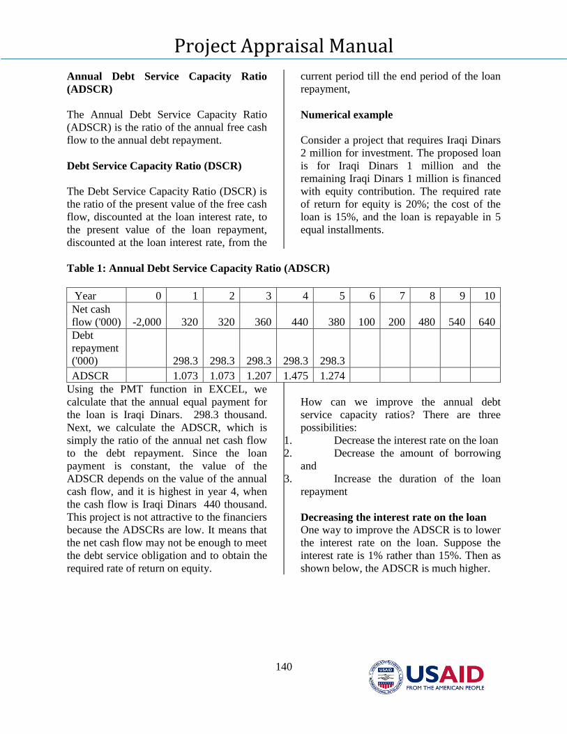
Project Appraisal Manual
140
Annual Debt Service Capacity Ratio
(ADSCR)
The Annual Debt Service Capacity Ratio
(ADSCR) is the ratio of the annual free cash
flow to the annual debt repayment.
Debt Service Capacity Ratio (DSCR)
The Debt Service Capacity Ratio (DSCR) is
the ratio of the present value of the free cash
flow, discounted at the loan interest rate, to
the present value of the loan repayment,
discounted at the loan interest rate, from the
current period till the end period of the loan
repayment,
Numerical example
Consider a project that requires Iraqi Dinars
2 million for investment. The proposed loan
is for Iraqi Dinars 1 million and the
remaining Iraqi Dinars 1 million is financed
with equity contribution. The required rate
of return for equity is 20%; the cost of the
loan is 15%, and the loan is repayable in 5
equal installments.
Table 1: Annual Debt Service Capacity Ratio (ADSCR)
Year 0 1 2 3 4 5 6 7 8 9 10
Net cash
flow ('000) -2,000 320 320 360 440 380 100 200 480 540 640
Debt
repayment
('000) 298.3 298.3 298.3 298.3 298.3
ADSCR 1.073 1.073 1.207 1.475 1.274
Using the PMT function in EXCEL, we
calculate that the annual equal payment for
the loan is Iraqi Dinars. 298.3 thousand.
Next, we calculate the ADSCR, which is
simply the ratio of the annual net cash flow
to the debt repayment. Since the loan
payment is constant, the value of the
ADSCR depends on the value of the annual
cash flow, and it is highest in year 4, when
the cash flow is Iraqi Dinars 440 thousand.
This project is not attractive to the financiers
because the ADSCRs are low. It means that
the net cash flow may not be enough to meet
the debt service obligation and to obtain the
required rate of return on equity.
How can we improve the annual debt
service capacity ratios? There are three
possibilities:
1. Decrease the interest rate on the loan
2. Decrease the amount of borrowing
and
3. Increase the duration of the loan
repayment
Decreasing the interest rate on the loan
One way to improve the ADSCR is to lower
the interest rate on the loan. Suppose the
interest rate is 1% rather than 15%. Then as
shown below, the ADSCR is much higher.
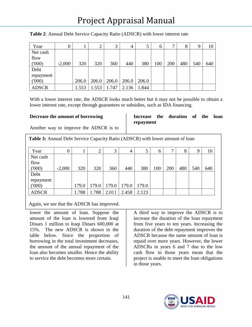
Project Appraisal Manual
141
Table 2: Annual Debt Service Capacity Ratio (ADSCR) with lower interest rate
Year 0 1 2 3 4 5 6 7 8 9 10
Net cash
flow
('000) -2,000 320 320 360 440 380 100 200 480 540 640
Debt
repayment
('000) 206.0 206.0 206.0 206.0 206.0
ADSCR 1.553 1.553 1.747 2.136 1.844
With a lower interest rate, the ADSCR looks much better but it may not be possible to obtain a
lower interest rate, except through guarantees or subsidies, such as IDA financing.
Decrease the amount of borrowing
Another way to improve the ADSCR is to
lower the amount of loan. Suppose the
amount of the loan is lowered from Iraqi
Dinars 1 million to Iraqi Dinars 600,000 at
15%. The new ADSCR is shown in the
table below. Since the proportion of
borrowing in the total investment decreases,
the amount of the annual repayment of the
loan also becomes smaller. Hence the ability
to service the debt becomes more certain.
Increase the duration of the loan
repayment
A third way to improve the ADSCR is to
increase the duration of the loan repayment
from five years to ten years. Increasing the
duration of the debt repayment improves the
ADSCR because the same amount of loan is
repaid over more years. However, the lower
ADSCRs in years 6 and 7 due to the low
cash flow in those years mean that the
project is unable to meet the loan obligations
in those years.
Table 3: Annual Debt Service Capacity Ratio (ADSCR) with lower amount of loan
Year 0 1 2 3 4 5 6 7 8 9 10
Net cash
flow
('000) -2,000 320 320 360 440 380 100 200 480 540 640
Debt
repayment
('000) 179.0 179.0 179.0 179.0 179.0
ADSCR 1.788 1.788 2.011 2.458 2.123
Again, we see that the ADSCR has improved.
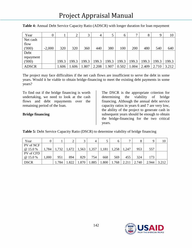
Project Appraisal Manual
142
Table 4: Annual Debt Service Capacity Ratio (ADSCR) with longer duration for loan repayment
Year 0 1 2 3 4 5 6 7 8 9 10
Net cash
flow
('000) -2,000 320 320 360 440 380 100 200 480 540 640
Debt
repayment
('000) 199.3 199.3 199.3 199.3 199.3 199.3 199.3 199.3 199.3 199.3
ADSCR 1.606 1.606 1.807 2.208 1.907 0.502 1.004 2.409 2.710 3.212
The project may face difficulties if the net cash flows are insufficient to serve the debt in some
years. Would it be viable to obtain bridge-financing to meet the existing debt payments in some
years?
To find out if the bridge financing is worth
undertaking, we need to look at the cash
flows and debt repayments over the
remaining period of the loan.
Bridge financing
The DSCR is the appropriate criterion for
determining the viability of bridge
financing. Although the annual debt service
capacity ratios in years 6 and 7 are very low,
the ability of the project to generate cash in
subsequent years should be enough to obtain
the bridge-financing for the two critical
years.
Table 5: Debt Service Capacity Ratio (DSCR) to determine viability of bridge financing
Year 0 1 2 3 4 5 6 7 8 9 10
PV of NCF
@ 15.0 % 1,784 1,732 1,672 1,563 1,357 1,181 1,258 1,247 953 557
PV of CFD
@ 15.0 % 1,000 951 894 829 754 668 569 455 324 173
DSCR 1.784 1.822 1.870 1.885 1.800 1.768 2.211 2.740 2.944 3.212
Project Appraisal Manual
143
Risk spreading and pooling
The most fundamental mechanism for
reducing (or even eliminating risk) is risk
spreading or pooling. As long as the
variation in a particular return is
unsystematic or unrelated to the other
returns, then the variation can be reduced in
line with the number of people sharing the
return. By spreading the risk across a pool of
persons (each owning a small share of the
risk), the variability can be reduced to zero
if the pool is large enough.
To understand the idea of risk spreading, we
discuss some basic variance relationships.
Let X and Y be two random variables, and
let a and b be constants.
Var(X) is the variance of X, Var(Y) is the
variance of Y and Cov(X,Y) is the
covariance of X and Y.
It is easy to show that the following
variance relationships hold.
Var(aX) = a2×Var(X) = a
2×(σX)
2
(1)
Var(aX + bY) = a2×Var(X) +
b2×Var(Y) + 2ab×Cov(X,Y)
= a2×(σX)
2 + b
2×(σY)
2 +
2ab×Cov(X,Y) (2)
The first relationship states that the variance
of constant times a random variable X
equals the square of the constant times the
variance of X. The second relationship
applies to the sum of two random variables.
Note the presence of the third term, which
includes the covariance between X and Y.
If X and Y are independent random
variables, then it means that they are
unrelated and the covariance between them
is zero. In this special case, we can simplify
equation 2 as follows.
Var(aX + bY) = a2×Var(X) + b
2×Var(Y)
= a2×(σX)
2 + b
2×(σY)
2 (3)
Now let R be the return on a new investment
project and let Var(R) be the variance of R.
Suppose there are N investors and the
investment project is equally divided among
the N investors. Then the variance for an
individual investor is just one nth of the
variance of R.
Variance for individual investor =
Var(R/N) (4.1)
The total variance for all of the
investors is as follows.
Total variance for all investors =
N×Var(R/N) (4.2)
We can rewrite equation 4.1 as
follows.
Total variance for all investors =
N×Var(R/N) = N×(1/N2)×Var(R) =
Var(R)/N (4.3)
Thus, we see that if the investment project is
shared or owned by N investors, then the
total variance for all the investors equals the
variance of the project divided by N. As N
gets large, the total variance tends towards
zero. However, the expected total return
remains the same.
Equation 6 is the basis for risk spreading or
pooling. The total variance of the
unsystematic risk declines towards zero as
the risk is spread among many investors.
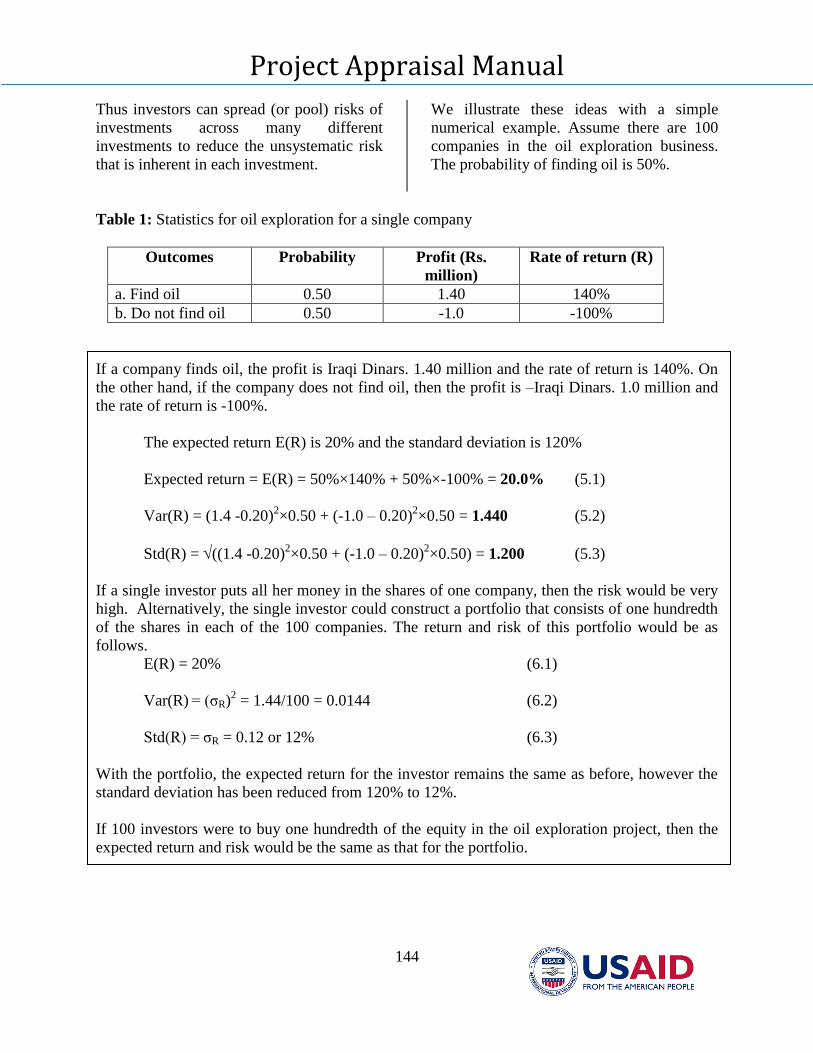
Project Appraisal Manual
144
Thus investors can spread (or pool) risks of
investments across many different
investments to reduce the unsystematic risk
that is inherent in each investment.
We illustrate these ideas with a simple
numerical example. Assume there are 100
companies in the oil exploration business.
The probability of finding oil is 50%.
Table 1: Statistics for oil exploration for a single company
Outcomes Probability Profit (Rs.
million)
Rate of return (R)
a. Find oil 0.50 1.40 140%
b. Do not find oil 0.50 -1.0 -100%
If a company finds oil, the profit is Iraqi Dinars. 1.40 million and the rate of return is 140%. On
the other hand, if the company does not find oil, then the profit is –Iraqi Dinars. 1.0 million and
the rate of return is -100%.
The expected return E(R) is 20% and the standard deviation is 120%
Expected return = E(R) = 50%×140% + 50%×-100% = 20.0% (5.1)
Var(R) = (1.4 -0.20)2×0.50 + (-1.0 – 0.20)
2×0.50 = 1.440 (5.2)
Std(R) = ((1.4 -0.20)2×0.50 + (-1.0 – 0.20)
2×0.50) = 1.200 (5.3)
If a single investor puts all her money in the shares of one company, then the risk would be very
high. Alternatively, the single investor could construct a portfolio that consists of one hundredth
of the shares in each of the 100 companies. The return and risk of this portfolio would be as
follows.
E(R) = 20% (6.1)
Var(R) = (σR)2 = 1.44/100 = 0.0144 (6.2)
Std(R) = σR = 0.12 or 12% (6.3)
With the portfolio, the expected return for the investor remains the same as before, however the
standard deviation has been reduced from 120% to 12%.
If 100 investors were to buy one hundredth of the equity in the oil exploration project, then the
expected return and risk would be the same as that for the portfolio.
Project Appraisal Manual
145
Systematic risk
Next, we explore the notion of systematic
risk and the relationship of the new project
investment to the existing portfolio of
investments. When a new investment is
undertaken, we need to distinguish between
the risk or variability in the return or NPV of
the new project and the impact that the
project has on the variability of the returns
of the entire portfolio of investments of the
investors in the project and the economy.
Systematic risk refers to the covariance (or
correlation) between the returns on the new
project and the returns on the existing
portfolio of investments of private investors
or all investments in the economy.
Investors demand a price or risk premium to
bear risk or variability in return. To reduce
the variability in returns of individual
investors, it is common practice to spread
the ownership among many owners. This
reduces the variability in returns from the
new project but necessarily in aggregate
when the variability is viewed in
conjunction with existing investments. It is
possible to show these concepts with basic
variance relationships.
Let ρXY be the correlation coefficient
between X and Y. Then the relationship
between the correlation coefficient and the
covariance is as follows.
ρXY = Cov(X,Y)/(σX×σY)
(7.1)
Solving for the covariance, we
obtain,
Cov(X,Y) = ρXY×σX×σY
(7.2)
From above, we know that,
Var(aX + bY) = a2×(σX)
2 + b
2×(σY)
2
+ 2ab×Cov(X,Y) (8.1)
Substituting equation 7.2 into
equation 8, we obtain,
Var(aX + bY) = a2×(σX)
2 + b
2×(σY)
2
+ 2ab×ρXY×σX×σY (8.2)
Regression analysis
From the standard OLS (Ordinary Least
Squares) regression analysis, we obtain the
following results. Assume that there is a
linear relationship between Y and X, where
ε is a random variable with a normal
distribution and zero mean.
Y = α + β×X + ε
(9)
The intercept is α and the slope coefficient is
β. We can show that the slope coefficient
equals the ratio of the covariance of X and
Y, and the variance of X.
β = Cov(X,Y)/Var(X)
(10)
Substituting the expression for the
covariance, we obtain the following
equation for the slope coefficient.
β = Cov(X,Y)/Var(X)
= ρXY×(σX)×(σY)/(σX)2 = ρXY×(σY/σX)
(11)
Project Appraisal Manual
146
Incremental systematic portfolio risk
To assess the impact on the risk of an
investor, it is necessary to check how the
new investment co-varies with the existing
portfolio and estimate the incremental
impact on the portfolio risk of the investor.
Let R be the return on the new investment
project and P is the return on the existing
portfolio. Then,
Var(R + P) = (σR)2 + (σP)
2 +
2ρRP×σR×σP (12.1)
Substituting the expression for the
slope coefficient, we obtain,
Var(R + P) = (σR)2 + (σP)
2 +
2β×(σP)2 (12.2)
The variance of the new project (σR)2, is the
variance resulting in the diversifiable risk
that can be reduced through risk pooling or
spreading. The covariance term gives the
incremental non-diversifiable or systematic
risk for the portfolio of the investor. The
systematic risk is a real unavoidable cost to
investors. The systematic risk is not reduced
if the government rather than the private
sector undertakes the project.
Mechanisms for reducing the costs of risk
There are four main mechanisms for
reducing the costs of risk. First, we can use
the capital, financial and futures markets.
Second, we can use contracts to reallocate or
share the cost of risk reduction. Third, there
are real options. And fourth, we can use
project finance.
Capital, financial and futures markets
Typically, investments are financed with a
combination of debt and equity. The
financing for a project can be raised in the
financial markets. The financial structure,
that is, the mix of debt and equity, results in
different payoff structures for the debt and
equity holders.
Contracting
To reduce the costs of risk, we can use
contracts to reallocate or share risks.
Contracts can change the internal
relationships to deal with exogenous market
variability, such as foreign exchange risk.
For example, contracts may use product
price formulas.
We can also use contracts to limit
exogenous market variability in prices and
quantities of raw materials.
Contracts are also relevant for changing the
internal relationships and thus change the
endogenous incentives. Examples include
profit sharing, stock options and other
flexible wage agreements. In addition, there
can be profit participation by the
construction contractor and operator.
Real options
With real options, we can design flexibility
into the project. The real options allow us to
respond to changes in information or market
conditions. There is a cost to the added
flexibility and thus we have to compare the
benefits of the flexibility with the cost of
increasing the flexibility in the project.
Project finance
Project finance consists of complex
contractual arrangements to deal with risk in
large investments. In non-recourse project
finance, the stakeholders in the project only
have claims to the cash flow that is
generated by the project. Thus, it is
important to structure the contracts in such a
Project Appraisal Manual
147
way that all the claimants to the cash flow
satisfy their required rates of return.
Capital Asset Pricing Model (CAPM)
If investors can establish well-diversified
portfolios and have a risk-free investment
available (such as a government bond), then
they can invest in a mix of the risk-free
investment and their investment portfolio.
If individual investors have no special
information, the portfolio of the individual
investor should be similar to the market
portfolio. Hence, investors can choose an
investment mix of the risk-free and market
portfolio which plots out the “market line”
running from the risk-free return through the
market return at the market standard
deviation. Therefore no investment should
pay a return that falls below this line given
the variability in its return.
Let rm be the return on the market portfolio
and rf be the risk-free rate. The market pays
a risk premium of (rm – rf), which is the
difference between the return on the market
and the risk-free rate. The risk premium paid
on any particular investment should be
proportional to its contribution to the market
portfolio risk premium. This relationship to
the market portfolio of the returns on any
investment (rj) is measured by its “beta” (βj).
Hence the CAPM is expressed as:
rj – rf = βj×(rm – rf) (1)
Or the return on any investment should be
the risk-free return plus its “beta” times the
market risk premium. The beta βj for any
investment “j” can be found by regressing
the returns for that type of investment on the
market return. In the extreme case, the risk-
free investment has a beta of zero, and as
expected, the return on the investment
equals the risk-free rate. On the other hand,
if the investment has a beta of one, then the
risk of the investment equals the risk of the
market portfolio.
Another perspective can be gained from the
following expression.
βj = ρj,market×(σj/σmarket) (2)
We can express the beta in terms of the
correlation between the investment and the
market portfolio ρj,market, the standard
deviation of the investment σj and the
standard deviation of the market σj. The
beta rises with the degree of correlation of
the return on investment “j” with the market
and the variance in the return on the
investment itself.
Risk allocation: sources of contracting
risks
In developing countries, well-developed
capital, financial and futures markets are not
always available. Investors can use contracts
to shift and share risks. Special contractual
arrangements are often required to mitigate
risks and make projects viable. We can view
contracts from either the cost perspective or
the efficiency perspective. The cost
perspective is implicitly a zero-sum
perspective. What one party gains, the other
party loses. An efficiency perspective is
explicitly a positive sum perspective. With
the right contract, one party may be able to
gain substantially without a corresponding
cost to the other party.
Risk shifting of exogenously generated
risks
First, investors have different risk
preferences. And a less risk-averse investor
may be willing to accept a lower return on a
risky asset. Second, different stakeholders
have different capacities to diversify. For
Project Appraisal Manual
148
example, foreign investors may have more
opportunities to diversify their investments
in efficient capital markets. Third, there are
differences in the outlooks, predictions and
information about the future. Some investors
may be more optimistic than others.
Contracts that restructure intra-project
correlations
Risk sharing can change the endogenous
incentives because different stakeholders
have differing ability to influence project
outcomes. We can use contracts to reduce
the risk profile of the project cash flow.
There are two possibilities. First, we can
structure risk-sharing contracts that reduce
the investors’ risk by increasing the
correlation between sales revenues and some
cost items. Examples include:
Profit sharing contracts with labor
Bonds with interest rates indexed to
producer sales price
Debt financing in the same currency
as the product sales
Product price indexed to major raw
materials price
Second, we can use contracts that decrease
the correlation between benefit items or
alternatively between cost items.
The formal demonstration of these ideas is
as follows. Earlier, we had presented the
following equation for the variance of two
random variables.
Var(aX + bY) = a2×Var(X) +
b2×Var(Y) + 2ab×Cov(X,Y)
= a2×(σX)
2 + b
2×(σY)
2 + 2ab×Cov(X,Y)
(3)
For our purposes, let X be the revenues R,
let Y be the costs C, let a equal 1, and let b
equal -1. Then we can rewrite equation 1 as
follows.
Var(Net profits) = Var(Y – C) =
Var(R) + Var(C) - 2×Cov(R,C) (4)
Any measure that increases the positive
correlation between revenues and costs will
increase the Cov(R, C), and in turn this
reduces the variance of the net profit
(provided of course that the measure does
not increase the variance of a cost item by
more than twice the change in the
covariance.)
Profit-sharing agreement with labor
Assume that wages are the only cost.
Without the agreement, the labor cost is C.
Next we examine the labor cost with
agreement. Let g be the proportion of the
costs that is still paid to workers as a fixed
part of the wage, and let h be the labor’s
share of profit after wages have been paid.
Thus total cost = g×C + h×(R - g×C)
(5)
Where the first term is the fixed wage and
the second term is the flexible wage.
Net profit = R - g×C - h×(R - g×C)
= (1 – h)×R – g×(1 – h)×C (6)
The expression for the variance of the net
profit is as follows,
Var(Net profit) = (1 – h)2×Var(R) + g
2×(1 –
h)2×Var(C) + Var(R) + 2×g×(1 –
h)×Cov(R,C) (7)
And if 0 < g < 1 and 0 < h < 1, then the
variance of net profit is lower than it is
without the wage agreement.
Project Appraisal Manual
149
Real options
Project design decisions that we make today
affect the flexibility in responding to
uncertain opportunities or constraints in the
future. We discuss several examples. First,
we could buy a larger land area than
currently needed. This would give us the
opportunity (or “real option” as compared to
a financial option) to expand the future
production of output in the event that
demand is stronger than expected. Second,
we could buy a more expensive machinery;
however, the higher cost of the equipment is
offset by the greater benefits that we obtain
from the flexibility in changing product lines
or using different types of materials.
Thirdly, we may forego the tax incentives to
enter an export processing zone because the
location in the export processing zone does
not allow us to sell in the domestic market
when there is a downturn in the export
market. Fourthly, we may prefer to have a
lower target debt-equity ratio to avoid debt
restructuring costs if there are declines in the
future cash flows.

Project Appraisal Manual
150
Summary of Project Appraisal Results
Project Appraisal Manual
151
SUMMARY OF PROJECT APPRAISAL RESULTS AND RECOMMENDTION FOR
ACTION
The following Table X.1 provides a summary of the basic results expected from the
appraisal of an investment project using the financial, economic, stakeholder and risk
analysis techniques discussed in the previous sections.
Table X.1 Summary of project appraisal results
Criterion or
Result
Primary or Basic Secondary
Self-financing
project
Non-self-
financing project
Economically
attractive?
NPV for
economy
NPVecon > 0. Also, IRR economic >
economic discount rate
NPVecon > 0 Also, IRR economic >
economic discount
rate
Probability of NPVecon <0, Standard deviation, maximum
and minimum values or
confidence intervals.
Sources of risk.
Financially
attractive to
equity holders or
sponsors?
NPV for equity
holders or
sponsors
NPVequity > 0. Also, IRR equity >
minimum required ROE
(return on equity)
NPVsponsor such that
injections of funds
are available in both
investment and
operating periods to
cover any negative
cash flows
Probability of NPVequity <0, Standard deviation, maximum
and minimum values or
confidence intervals.
Sources of risk,
Impacts of risk sharing
contracts, sales or purchase
agreements.
Financially
attractive to
combined
financiers?
NPV to total
investment
NPVtotal investment > 0.
NPVtotal investment =
NPVequity. Also, IRR total
investment > minimum
required return on
investment ROI
(WACC)
Adequate debt coverage
ratios or sufficiently low
probability of default
relative to default premium
charged
NPV to
stakeholders
consistent with
NPV for
economy
NPVecon = sum of NPV
to stakeholders
NPVecon = sum of
NPV to stakeholders
NPV to key
stakeholders
NPV to equity holders,
NPV to adversely
affected groups
through environmental
impacts, labor
adjustment or social
dislocation
NPV to target
beneficiary group,
particularly for
social program
delivering basic
needs
Standard deviation, maximum
and minimum values or
confidence intervals.
NPV of target group relative
to NPV economy: win-win or
target groups wins at expense
of economy?
Project Appraisal Manual
152
Based on the set of results
derived from a comprehensive
analysis of an investment project
the following is the typical range
of recommendations:
1. For a self-financing project, where it
is:
1.1 both financially and
economically attractive with
manageable risks and no key
stakeholder group expected to
experience major unintended
gains or losses, the project
should proceed as designed.
1.2 subject to government regulation
or participation agreements and
is economically attractive and
excessively attractive to the
private investors, the project
should proceed but with
reduced gains to the private
investors through adjusting
contract prices or otherwise
renegotiating the agreements.
1.3 economically attractive, but
financially unattractive to the
stakeholders, the regulated
prices or contract agreement
should be adjusted to make the
contract sufficiently attractive
to the private investors by
adjusting prices and/or
introducing risk sharing
arrangements to reallocate risks
and/or improve performance
incentives.
1.4 financially attractive, but
economically unattractive (as
may occur in a protected or
subsidized sector), the degree
of protection or subsidy should
be reduced such that the
investment becomes
economically attractive, if
feasible.
1.5 both financially and
economically unattractive, it
should be reconsidered for
project redesign – changed
scale, timing, technology, real
options, and/or financial and
contractual arrangements – to
assess whether the project can
be made attractive under new
design parameters or
agreements.
2. For a non-self-financing project,
where it is
2.1 economically attractive, has
secure operational finances and
the target beneficiary group
experiences intended gains
(typically from added supply of
a basic need), and no key
stakeholder group expected to
experience major losses, the
project should proceed as
designed.
2.2 economically attractive, but has
insecure operational finances, it
should be reassessed based on
reduced production of services
and beneficiary gains to assess
whether it remains
economically attractive under
realistic financing levels for its
operations; otherwise it should
be deferred until financing of
its operations can be assured.
2.3 economically unattractive, has
secure operational finances and
the target beneficiary group
experiences intended gains
(typically from added supply of
Project Appraisal Manual
153
a basic need), the project
should be considered for
redesign to determine whether
at a different scale or with a
different technology it can
deliver adequate benefits to the
target stakeholders, but with
either positive economic gains
or limiting the economic losses
to a small share (say below
20%) of the gains of the target
group; otherwise reject the
project18
.
18
The beneficiary group could be assisted with a
cash transfer equal to their expected gain less the
economic cost of raising and administering the funds
transferred (typically about 20% of the funds.)

Project Appraisal Manual
154
Appendixes
Project Appraisal Manual
155
Appendix 1: Economic Externalities
Introduction
In an economy where there are no taxes,
subsidies, or market imperfections such as
monopoly, external costs/benefits (pollution,
congestion, common-property), at the
margin there is no divergence between the
value of a good or service as manifested by
its demand price and the cost of production
as represented by the supply price. In this
kind of ideal world, the financial and
economic prices of outputs and inputs are
the same and there is no difference between
the financial appraisal of an investment and
its economic evaluation. These distortions
and imperfections, however, exist in real
markets and can be the source of external
welfare effects that should be taken into
account while estimating the economic
impacts of production or use of a product by
the project.
Economic externalities are said to exist
when the economic value of a product is
different from its financial price. For
example, to the extent that the economic
benefit (value) to the society of the
incremental output of a project is greater
than the financial price received by the
project owners, a positive externality is
created. When building up the economic
benefits from the financial receipts, all
externalities should be added to the financial
receipts. Similarly, if the economic costs of
the resources required by a project exceed
their financial cost, a negative externality is
created that should be added to the financial
expenditures incurred by the project. Annex
IV presents an example of the different
types of externalities that one may usually
come across while appraising a project and
also demonstrates how they are accounted
for in moving from the financial to the
economic analysis.
In some circumstances externalities could
also arise due to the impact of the project on
other industries, particularly industries
producing close complementary and
substitute goods, or externality might exist
in industries producing inputs to the
intermediate goods used by the project. If
industries producing complementary or
substitute goods experience changes in
demand or supply, which in turn lead to a
price change or a change in government
revenues, an externality is created. One
should carefully analyze the situation to
determine whether the impact on substitutes
and complements is expected to be small
and could be ignored for practical purposes,
or is large and should be included in the
analysis.19
Similarly, if an externality exists
in the market for one of the inputs of an
intermediate good required by a project and
it is sufficiently large, it would be necessary
to include it in the analysis.
What is Economic Externality?
All the distortions and imperfections in the
markets for both traded and non-traded
goods or services may be included in the
term “economic externality” defined in a
broader sense. Economic externality arises
because of a divergence between the
marginal social value and the marginal
19
For a detailed analysis of incorporating the impacts
of a project on complementary and substitute
markets, see Harberger, A. and Jenkins, GP.,
“Manual for Cost Benefit Analysis of Investment
Decisions”, Unpublished, Chapter 11, Section 3
(HIID, Harvard University 2005)
Project Appraisal Manual
156
social cost of activities whose demand or
supply is affected by a project. While
physical or technological externalities refer
to effects like noise, pollution or congestion,
the term “economic externality” would
cover all potential sources of external
welfare effects that have been described
above. With this connotation, “economic
externality” may be defined as follows.
An externality or external economy
(diseconomy) is an occurrence or incident
that confers benefits (damages) on some
persons who are not fully consenting parties
in reaching the decision that gives rise to the
event in question20
.
It may be noted that an economic externality
arises when the persons affected were not
fully consenting parties to the decision. For
instance, in case of taxes and subsidies the
affected individuals might have been a party
to the process leading to the installation of
the government (voting), but they are not a
party to the institutional process through
which these measures are approved. As a
result, each time that a project causes a
change in the level of a taxed activity that
yields more or less tax revenues to the
government, an externality arises.
There are several situations where an
economic externality may arise. Some of the
cases of externalities that are of relevance
while appraising a project are described
below.
Environmental Externalities
20
This definition is due to James E. Meade; “The
Theory of Economic Externalities”, Institut
Universitaire de Hautes Etudes Internationales,
Geneva (1973).
Environmental externality is generated when
the external diseconomy arises as a result of
the production process of a project. The
different kinds of pollution created by
industrial firms and infrastructure projects
(power, transport) in the process of
producing goods and services fall in this
category. A lot of waste products or
effluents are deposited in the atmosphere,
waterways and the ground by some projects.
This has a damaging effect on people and
property that are not directly involved with
the production or consumption of the output.
Accounting for Environmental Externalities
in Project Appraisal
Whenever an investment has an adverse
impact on the environment, there are two
steps to incorporate this effect into project
evaluation. First, the cost of measures
necessary to reduce or eliminate the impact
should be part of the project and the costs of
those measures should be included both in
the financial and economic analyses of the
project. These measures may include
alterations in the existing plant or adding
some new equipment. If the impact on the
environment cannot be totally eliminated, as
would generally be the case, then the
damage caused by the residual impact
should be estimated and added as a cost in
the economic analysis of the project. This
evaluation of the residual impact on the
environment and consequently on the people
may not be always straightforward and may
often require special evaluation techniques.
Monopoly Externalities
Sometimes there is only one producer of a
good or service in the economy and he
enjoys a monopoly in the market. The
monopolist is in a position to set the price
Project Appraisal Manual
157
and then sell the output that is demanded by
the consumers at that price. From an
alternative perspective, the monopolist can
restrict the output which will raise the price
of the good/service in the market over and
above its marginal cost of production21
.
Compared to the situation in a competitive
market, the amount of the good/service
transacted in the market is lower and the
price is higher. As a result, consumers lose
and the producer gains at the cost of
consumers. The determination of price and
quantity in a monopoly market is depicted in
the figure below.
A monopoly may arise due to a variety of
reasons. There may be a single owner of a
resource that is crucial to the production
process; there may be some legal or
institutional barriers to the entry of other
producers; or there may exist a natural
monopoly arising from economies of large
scale production that leaves no scope for
more than one producer22
.
21
This price difference is sometimes referred to as a
monopoly tax. The consumers have to pay a higher
price compared to the situation in a competitive
market as if the monopolist is imposing a tax on
them. As a consequence, the consumer surplus
declines and the producer surplus is higher. 22
The single ownership situation may arise in case of
natural resources. The legal/institutional barriers
often have their origin in some patent law. The
natural monopoly occurs in case of large scale
utilities such as railways and telecommunications.
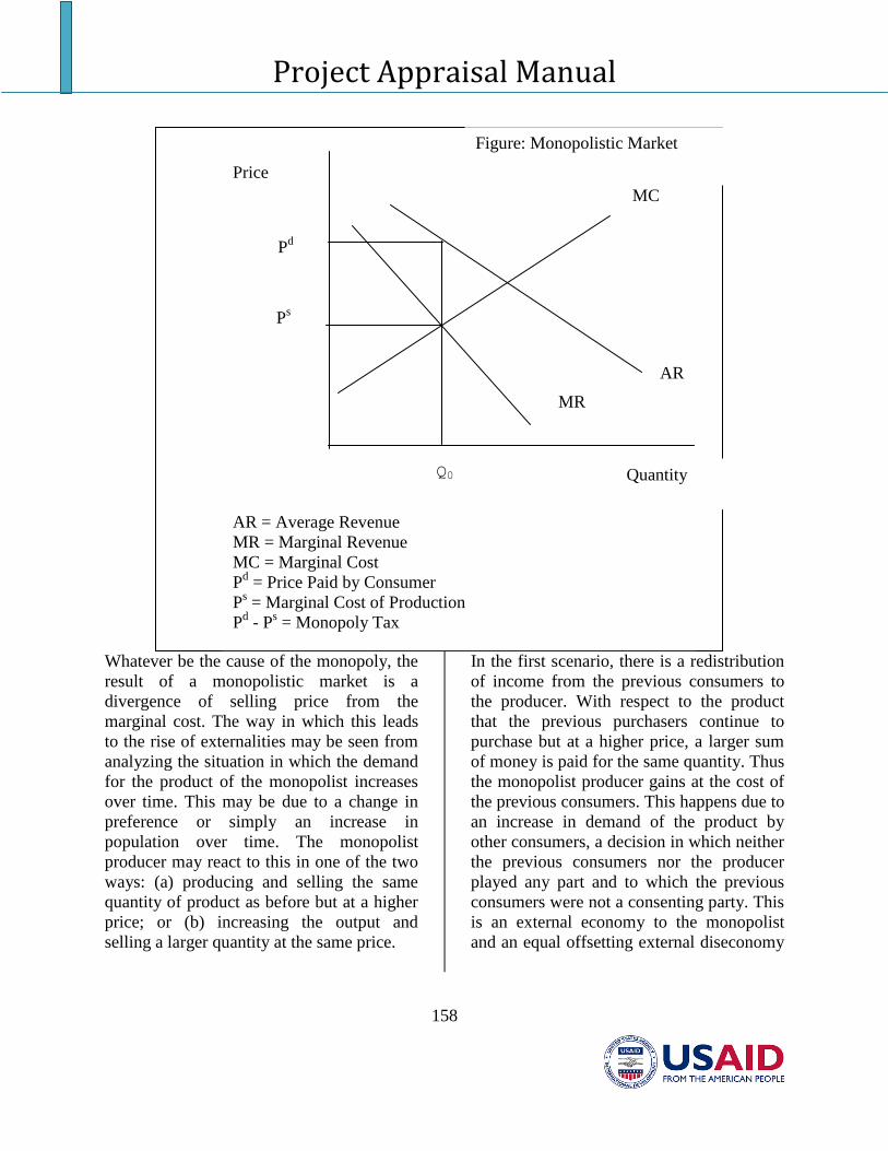
Project Appraisal Manual
158
Whatever be the cause of the monopoly, the
result of a monopolistic market is a
divergence of selling price from the
marginal cost. The way in which this leads
to the rise of externalities may be seen from
analyzing the situation in which the demand
for the product of the monopolist increases
over time. This may be due to a change in
preference or simply an increase in
population over time. The monopolist
producer may react to this in one of the two
ways: (a) producing and selling the same
quantity of product as before but at a higher
price; or (b) increasing the output and
selling a larger quantity at the same price.
In the first scenario, there is a redistribution
of income from the previous consumers to
the producer. With respect to the product
that the previous purchasers continue to
purchase but at a higher price, a larger sum
of money is paid for the same quantity. Thus
the monopolist producer gains at the cost of
the previous consumers. This happens due to
an increase in demand of the product by
other consumers, a decision in which neither
the previous consumers nor the producer
played any part and to which the previous
consumers were not a consenting party. This
is an external economy to the monopolist
and an equal offsetting external diseconomy
MC
AR
Q0
Ps
Pd
Quantity
Price
Figure: Monopolistic Market
AR = Average Revenue
MR = Marginal Revenue
MC = Marginal Cost
Pd = Price Paid by Consumer
Ps = Marginal Cost of Production
Pd - P
s = Monopoly Tax
MR
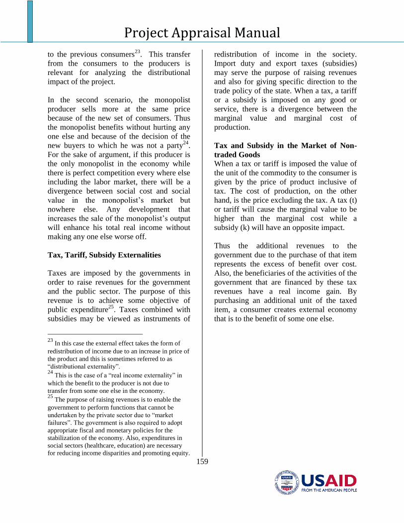
Project Appraisal Manual
159
to the previous consumers23
. This transfer
from the consumers to the producers is
relevant for analyzing the distributional
impact of the project.
In the second scenario, the monopolist
producer sells more at the same price
because of the new set of consumers. Thus
the monopolist benefits without hurting any
one else and because of the decision of the
new buyers to which he was not a party24
.
For the sake of argument, if this producer is
the only monopolist in the economy while
there is perfect competition every where else
including the labor market, there will be a
divergence between social cost and social
value in the monopolist’s market but
nowhere else. Any development that
increases the sale of the monopolist’s output
will enhance his total real income without
making any one else worse off.
Tax, Tariff, Subsidy Externalities
Taxes are imposed by the governments in
order to raise revenues for the government
and the public sector. The purpose of this
revenue is to achieve some objective of
public expenditure25
. Taxes combined with
subsidies may be viewed as instruments of
23
In this case the external effect takes the form of
redistribution of income due to an increase in price of
the product and this is sometimes referred to as
“distributional externality”. 24
This is the case of a “real income externality” in
which the benefit to the producer is not due to
transfer from some one else in the economy. 25
The purpose of raising revenues is to enable the
government to perform functions that cannot be
undertaken by the private sector due to “market
failures”. The government is also required to adopt
appropriate fiscal and monetary policies for the
stabilization of the economy. Also, expenditures in
social sectors (healthcare, education) are necessary
for reducing income disparities and promoting equity.
redistribution of income in the society.
Import duty and export taxes (subsidies)
may serve the purpose of raising revenues
and also for giving specific direction to the
trade policy of the state. When a tax, a tariff
or a subsidy is imposed on any good or
service, there is a divergence between the
marginal value and marginal cost of
production.
Tax and Subsidy in the Market of Non-
traded Goods
When a tax or tariff is imposed the value of
the unit of the commodity to the consumer is
given by the price of product inclusive of
tax. The cost of production, on the other
hand, is the price excluding the tax. A tax (t)
or tariff will cause the marginal value to be
higher than the marginal cost while a
subsidy (k) will have an opposite impact.
Thus the additional revenues to the
government due to the purchase of that item
represents the excess of benefit over cost.
Also, the beneficiaries of the activities of the
government that are financed by these tax
revenues have a real income gain. By
purchasing an additional unit of the taxed
item, a consumer creates external economy
that is to the benefit of some one else.
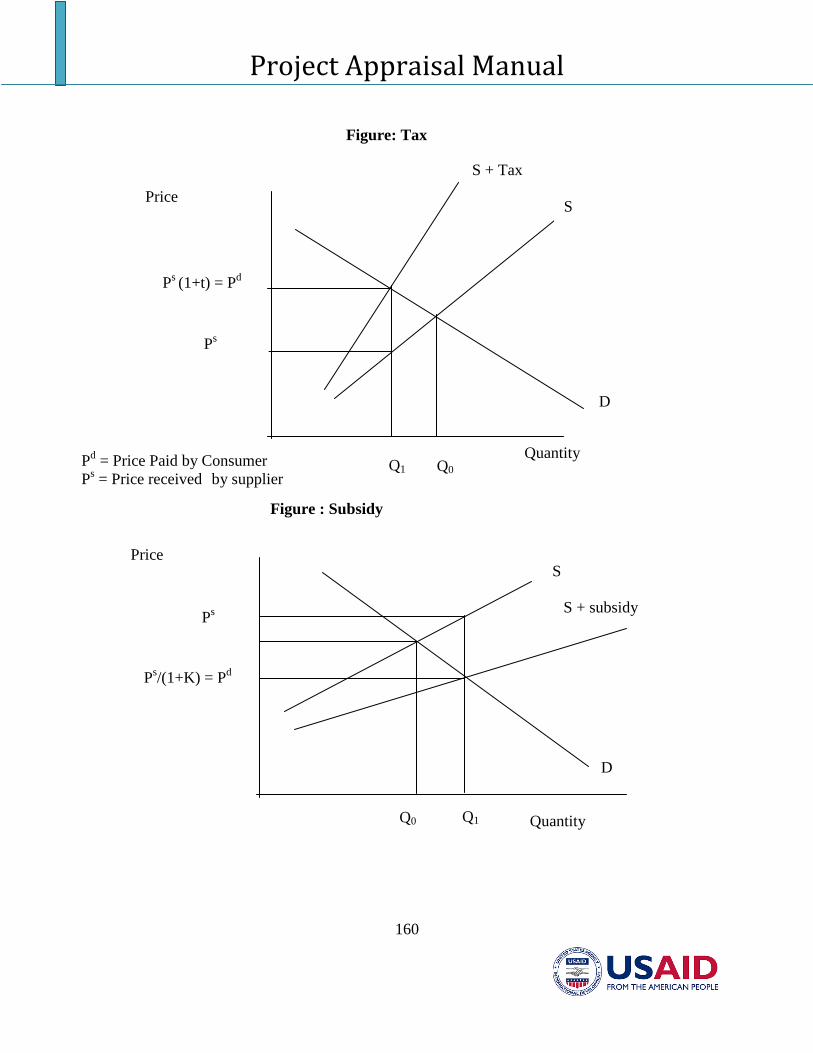
Project Appraisal Manual
160
Quantity Q1 Q0
D
S
S + Tax
Ps (1+t) = P
d
Ps
Price
Figure: Tax
Pd = Price Paid by Consumer
Ps = Price received by supplier
Q0 Q1
Ps
Ps/(1+K) = P
d
S
S + subsidy
Price
Quantity
D
Figure : Subsidy
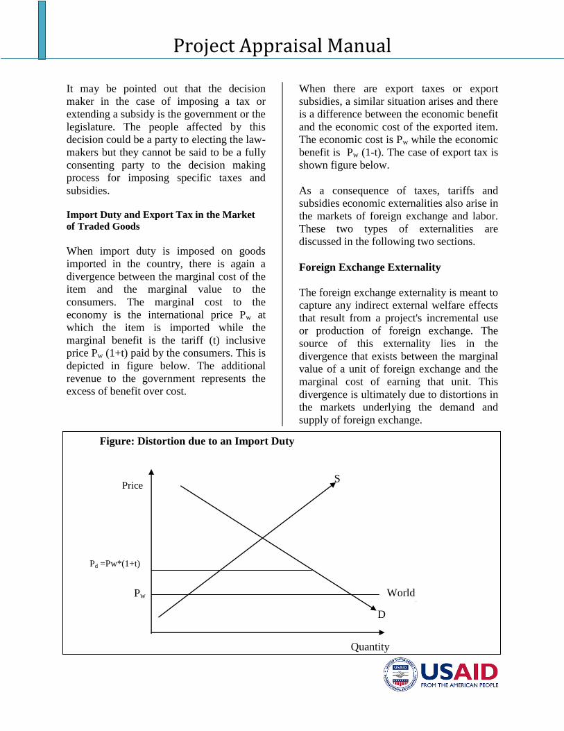
Project Appraisal Manual
161
It may be pointed out that the decision
maker in the case of imposing a tax or
extending a subsidy is the government or the
legislature. The people affected by this
decision could be a party to electing the law-
makers but they cannot be said to be a fully
consenting party to the decision making
process for imposing specific taxes and
subsidies.
Import Duty and Export Tax in the Market
of Traded Goods
When import duty is imposed on goods
imported in the country, there is again a
divergence between the marginal cost of the
item and the marginal value to the
consumers. The marginal cost to the
economy is the international price Pw at
which the item is imported while the
marginal benefit is the tariff (t) inclusive
price Pw (1+t) paid by the consumers. This is
depicted in figure below. The additional
revenue to the government represents the
excess of benefit over cost.
When there are export taxes or export
subsidies, a similar situation arises and there
is a difference between the economic benefit
and the economic cost of the exported item.
The economic cost is Pw while the economic
benefit is Pw (1-t). The case of export tax is
shown figure below.
As a consequence of taxes, tariffs and
subsidies economic externalities also arise in
the markets of foreign exchange and labor.
These two types of externalities are
discussed in the following two sections.
Foreign Exchange Externality
The foreign exchange externality is meant to
capture any indirect external welfare effects
that result from a project's incremental use
or production of foreign exchange. The
source of this externality lies in the
divergence that exists between the marginal
value of a unit of foreign exchange and the
marginal cost of earning that unit. This
divergence is ultimately due to distortions in
the markets underlying the demand and
supply of foreign exchange.
Figure: Distortion due to an Import Duty
Price
Pd =Pw*(1+t)
Pw
S
D
World Supply
Quantity
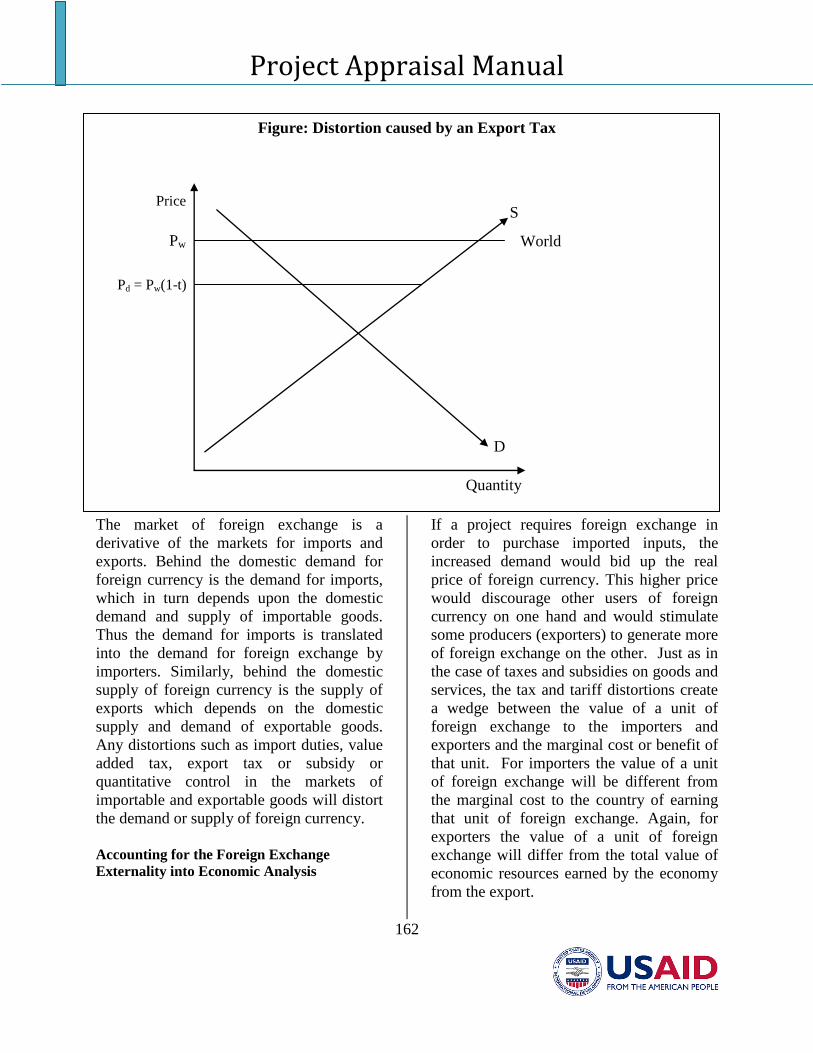
Project Appraisal Manual
162
Figure: Distortion caused by an Export Tax
The market of foreign exchange is a
derivative of the markets for imports and
exports. Behind the domestic demand for
foreign currency is the demand for imports,
which in turn depends upon the domestic
demand and supply of importable goods.
Thus the demand for imports is translated
into the demand for foreign exchange by
importers. Similarly, behind the domestic
supply of foreign currency is the supply of
exports which depends on the domestic
supply and demand of exportable goods.
Any distortions such as import duties, value
added tax, export tax or subsidy or
quantitative control in the markets of
importable and exportable goods will distort
the demand or supply of foreign currency.
Accounting for the Foreign Exchange
Externality into Economic Analysis
If a project requires foreign exchange in
order to purchase imported inputs, the
increased demand would bid up the real
price of foreign currency. This higher price
would discourage other users of foreign
currency on one hand and would stimulate
some producers (exporters) to generate more
of foreign exchange on the other. Just as in
the case of taxes and subsidies on goods and
services, the tax and tariff distortions create
a wedge between the value of a unit of
foreign exchange to the importers and
exporters and the marginal cost or benefit of
that unit. For importers the value of a unit
of foreign exchange will be different from
the marginal cost to the country of earning
that unit of foreign exchange. Again, for
exporters the value of a unit of foreign
exchange will differ from the total value of
economic resources earned by the economy
from the export.
Pd = Pw(1-t)
Pw World Demand
Price
Quantity
S
D
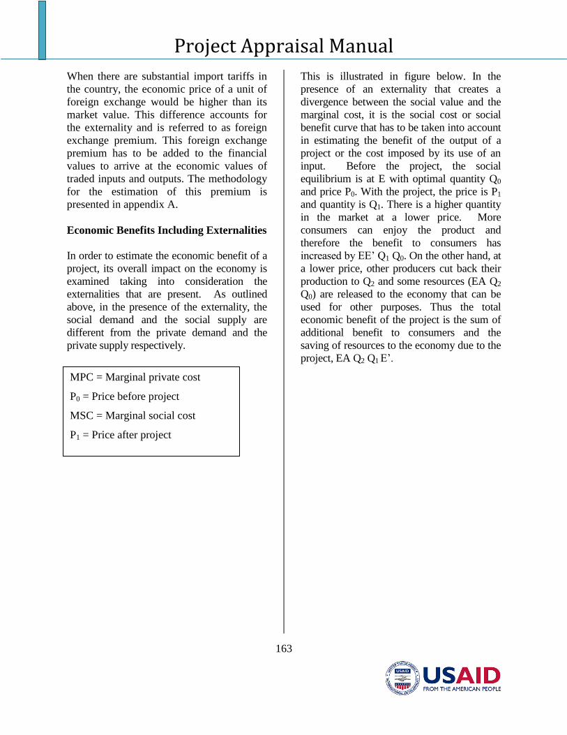
Project Appraisal Manual
163
When there are substantial import tariffs in
the country, the economic price of a unit of
foreign exchange would be higher than its
market value. This difference accounts for
the externality and is referred to as foreign
exchange premium. This foreign exchange
premium has to be added to the financial
values to arrive at the economic values of
traded inputs and outputs. The methodology
for the estimation of this premium is
presented in appendix A.
Economic Benefits Including Externalities
In order to estimate the economic benefit of a
project, its overall impact on the economy is
examined taking into consideration the
externalities that are present. As outlined
above, in the presence of the externality, the
social demand and the social supply are
different from the private demand and the
private supply respectively.
This is illustrated in figure below. In the
presence of an externality that creates a
divergence between the social value and the
marginal cost, it is the social cost or social
benefit curve that has to be taken into account
in estimating the benefit of the output of a
project or the cost imposed by its use of an
input. Before the project, the social
equilibrium is at E with optimal quantity Q0
and price P0. With the project, the price is P1
and quantity is Q1. There is a higher quantity
in the market at a lower price. More
consumers can enjoy the product and
therefore the benefit to consumers has
increased by EE’ Q1 Q0. On the other hand, at
a lower price, other producers cut back their
production to Q2 and some resources (EA Q2
Q0) are released to the economy that can be
used for other purposes. Thus the total
economic benefit of the project is the sum of
additional benefit to consumers and the
saving of resources to the economy due to the
project, EA Q2 Q1 E’.
MPC = Marginal private cost
P0 = Price before project
MSC = Marginal social cost
P1 = Price after project
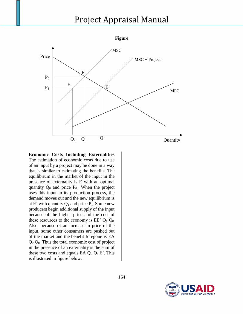
Project Appraisal Manual
164
Figure
Economic Costs Including Externalities
The estimation of economic costs due to use
of an input by a project may be done in a way
that is similar to estimating the benefits. The
equilibrium in the market of the input in the
presence of externality is E with an optimal
quantity Q0 and price P0. When the project
uses this input in its production process, the
demand moves out and the new equilibrium is
at E’ with quantity Q1 and price P1. Some new
producers begin additional supply of the input
because of the higher price and the cost of
these resources to the economy is EE’ Q1 Q0.
Also, because of an increase in price of the
input, some other consumers are pushed out
of the market and the benefit foregone is EA
Q2 Q0. Thus the total economic cost of project
in the presence of an externality is the sum of
these two costs and equals EA Q2 Q1 E’. This
is illustrated in figure below.
Price
Quantity
P0
P1
E
A E’
MSC
MSC + Project
MPC
Q0 Q1 Q2
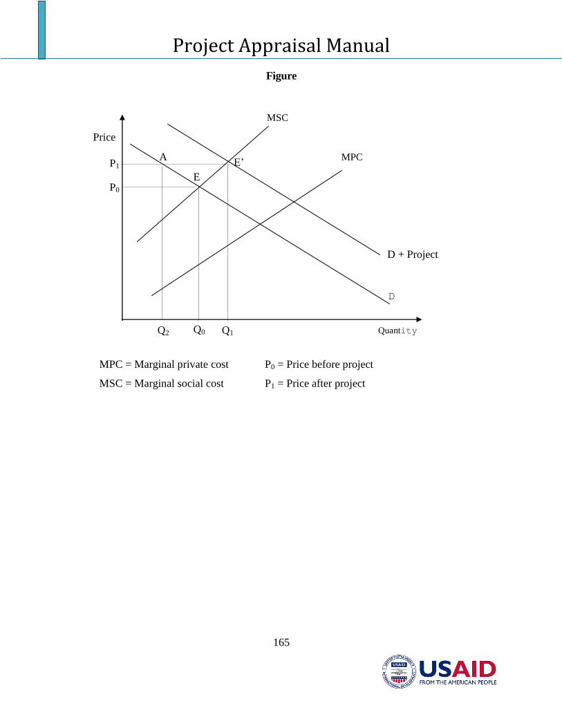
Project Appraisal Manual
165
Figure
MPC = Marginal private cost P0 = Price before project
MSC = Marginal social cost P1 = Price after project
Price
Quantity
P0
P1
E
A E’
MSC
D + Project
MPC
D
Q0 Q1 Q2
Project Appraisal Manual
166
Economic Externalities in the Capital
Market and the Labor Market
The distortions in the capital market in the
form of taxes and subsidies on return to
savings (personal income taxes) and
investment (property tax, corporate income
tax) cause a divergence between the
financial cost of capital (financial discount
rate) and the Economic Opportunity Cost of
Capital (EOCL or the economic discount
rate) which is to be used for applying the
investment criteria while conducting
economic analysis of a project. The
methodology for estimation of opportunity
cost of capital is presented in appendix B.
Similarly, there are distortions in the labor
market (income taxes, minimum wages) that
create a distortion between the financial
wage and the economic wage. While the
market wage rate is used in conducting
financial analysis of a project, the economic
cost of labor has to be used in economic
analysis. The methodology for estimating
the economic cost of labor (EOCL) is
presented in appendix C.
Project Appraisal Manual
167
Annex IV
Different Types of Externalities and Accounting for Them in the Economic Analysis
The various externalities that one may often
come across in appraising a project are
described in table below (middle column).
Also the relationship between the financial
analysis and the economic analysis is
summarized in this table. Column 1
presents the itemized incremental expected
cash flows from the perspective of all
investors. The bottom line for the financial
analysis is measured by the NPV of the
incremental expected net cash flows to total
capital discounted by the private discount
rate, i.e., the weighted average cost of
capital (WACC) for that project.
Column 2 lists the various adjustments and
externalities that need to be made to the
financial analysis in order to turn it into an
economic analysis. The adjustments
account for any change in consumers’
surplus and/or economic rent.
Column 3 includes the estimates of
incremental economic benefits and costs.
There are two ways of achieving these
estimates, namely: (a) use Harberger’s three
principles or postulates of willingness to
pay, supply price, and “a Dinar is a Dinar”
to measure economic benefits and costs
directly, or (b) add the appropriate
adjustment or externality to the
corresponding financial cash flows to
measure economic benefits and costs
indirectly. The economic externality
associated with each of the cash flow items
is simply the difference between the
economic price and market price of that item
For example, cash receipts and expenditures
on materials, machinery and equipment in
table below are divided into those arising
from the sale and purchase of tradable and
non-tradable commodities. The sale and
purchase of tradable commodities will
generate tariff and tax externalities as well
as a foreign exchange externality. The latter
is due to distortions in the markets for the
country’s all tradable and non-tradable
commodities, not just in the market for the
project’s inputs and output that cause the
economic opportunity cost of foreign
exchange (economic exchange rate) to differ
from the market exchange rate. The effect
of adding the foreign exchange externality to
the domestic value of the incremental
foreign exchange generated by either a
project’s exports or its import substitution,
as in approach (b) above, is equivalent to
valuing the incremental foreign exchange by
the economic exchange rate, as in approach
(a). Similarly, the foreign exchange
externality should be added to the domestic
cost of foreign exchange required for
tradable materials, machinery and
equipment.
Using approach (a), the economic benefit of
a project’s non-tradable output is measured
by the economic value of any incremental
industry output and consumption (based on
willingness to pay) and/or by the economic
value of any resources (based on their
supply price) released by other firms in the
industry that are forced to reduce their
output or shut down in response to a
project’s increased output. Let us say that a

Project Appraisal Manual
168
project’s output just creates incremental
industry output and consumption. If the
output is subject to a sales tax such that the
price paid by consumers inclusive of the tax
is higher than the price received by
producers, then the economic value of any
incremental output (based on willingness to
pay) will include the incremental sales tax
revenue (i.e. approach (a)). The alternative
approach (b) recognizes that the sales tax is
a market distortion that creates a sales tax
externality that should be added to the
private sector cash receipts to measure a
project’s economic benefits.
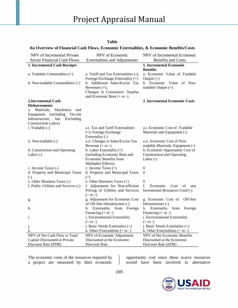
Project Appraisal Manual
169
Table
An Overview of Financial Cash Flows, Economic Externalities, & Economic Benefits/Costs
NPV of Incremental Private
Sector Financial Cash Flows
NPV of Economic
Externalities and Adjustments
NPV of Incremental Economic
Benefits and Costs
1. Incremental Cash Receipts
1. Incremental Economic
Benefits a. Tradable Commodities (+) a. Tariff and Tax Externalities (-);
Foreign Exchange Externality (+)
a. Economic Value of Tradable
Output (+)
b. Non-tradable Commodities (+) b. Additional Sales/Excise Tax
Revenues (+);
b. Economic Value of Non-
tradable Output (+)
Changes in Consumers’ Surplus
and Economic Rent (+ or -)
2.Incremental Cash
Disbursements
2. Incremental Economic Costs
a. Materials, Machinery and
Equipment (including On-site
Infrastructure, but Excluding
Construction Labor)
i. Tradable (-) a.i. Tax and Tariff Externalities
(+); Foreign Exchange
Externality (-)
a.i. Economic Cost of Tradable
Materials and Equipment (-)
ii. Non-tradable (-) a.ii. Changes is Sales/Excise Tax
Revenue (+ or -)
a.ii. Economic Cost of Non-
tradable Materials, Equipment (-)
b. Construction and Operating
Labor (-)
b. Labor Externality (+)
(including Economic Rent and
Economic Benefits from
Multiplier Effects)
b. Economic Opportunity Cost of
Construction and Operating
Labor (-)
c. Income Taxes (-) c. Income Taxes (+) 0
d. Property and Municipal Taxes
(-)
d. Property and Municipal Taxes
(+)
0
e. Other Business Taxes (-) e. Other Business Taxes (+) 0
f. Public Utilities and Services (-) f. Adjustment for Non-efficient
Pricing of Utilities and Services
(+ or -)
f. Economic Cost of any
Incremental Resources Used (-)
g. g. Adjustment for Economic Cost
of Off-Site Infrastructure (-)
g. Economic Cost of Off-Site
Infrastructure (-)
h. h. Externality from Foreign
Financing (+ or -)
h. Externality from Foreign
Financing (+ or -)
i. i. Environmental Externality
(+ or -)
i. Environmental Externality
(+ or -)
j. j. Basic Needs Externality (+) j. Basic Needs Externality (+)
k. k. Other Externalities (+ or -) k. Other Externalities (+ or -)
NPV of Net Cash Flow to Total
Capital Discounted at Private
Discount Rate (PDR)
NPV of Economic Adjustment
Discounted at the Economic
Discount Rate
NPV of Net Economic Benefits
Discounted at the Economic
Discount Rate (EDR)
The economic costs of the resources required by
a project are measured by their economic
opportunity cost since these scarce resources
would have been involved in alternative
Project Appraisal Manual
170
activities in the absence of a project. When the
resources would otherwise have been employed,
then their opportunity cost is measured by the
willingness of other users to pay for their use in
their forgone employment. When the resources
have to be attracted to this industry from
elsewhere in the economy, then their supply
price becomes the economic opportunity cost.
And when resources are drawn from both other
employment and other activities, then the
economic opportunity cost is a weighted average
of the willingness to pay in the forgone
employment and the minimum supply price.
As on the output side, any difference between
the economic opportunity costs of the resources
employed by a project and their market cost, can
be considered an economic externality. Hence,
there are two ways in which to estimate the
economic opportunity cost of a project’s inputs,
namely: (a) use Harberger’s principles of
willingness to pay, supply price, and “a Dinar is
a Dinar” to measure economic costs directly, or
(b) estimate the appropriate adjustment or
economic externality and add it to the
corresponding financial cash outflows. The
adjustment that might have to be made in this
case is to include any economic rent that is
earned by the owners of an input; this rent is
comparable to any change in consumers’ surplus
on the output side.
Taxes paid by a firm as a result of a project such
as income tax, property and municipal tax and
other business taxes are a private cost, but not
necessarily a cost to the economy. This is why
items (c), (d) and (e) under cash disbursements
have an economic cost of zero.
In addition to these immediate externalities there
is a broader set of external effects that also has
to be taken into account in the economic
analysis.
The financial price of utilities is often fixed
by the government and it may be quite different
from its economic value.
The firm proposing a project considers only the
private cost of any required on-site infrastructure
whereas the economic analysis should include
the economic cost of both the on-site and off-site
infrastructure, such as improved transportation
facilities or the added capacity of public utilities.
Foreign debt or equity financing may generate
added economic benefits or costs not included in
the financial appraisal.
A project may cause increased environmental
damage which is excluded from the private
financial analysis, but should be included as an
economic cost.
A project may create a basic needs externality if
it improves the provision of basic needs to the
most needy segments of society.
The estimates of incremental economic benefits
and costs should be discounted by an economic
discount rate. Since economic benefits and costs
can estimated by adding economic externalities
to their corresponding financial cash flows, both
the externalities and the financial cash flows
have to be discounted by the economic discount
rate as well.
Project Appraisal Manual
171
Appendix 2: Estimation of Economic Prices or Tradable Goods and Services
Introduction
Projects affect economic well-being in a
country. To analyze the economic worth of a
project it is important to know the true
economic values of its inputs and outputs. In
order to get these true economic values we
need to know:
1. Whether the goods are tradable or non-
tradable;
2. How distortions such as tariffs, taxes, and
subsidies create a wedge between economic
and financial values of both tradable and non-
tradable project’s inputs and outputs;
3. How the transportation and handling costs of
inputs and outputs affect the true economic
values of goods and services used and
produced by a project;
4. How distortions also create a divergence
between the market and the economic
exchange rates, the financial and economic
costs of capital and financial and economic
wage rates.
This chapter explains the above concepts and
shows in detail how to obtain the true
economic prices of tradable goods and
services.
Project appraisal emphasizes the difference
between the financial and economic values
of inputs and outputs particularly when
distortions exist in either the demand or
supply side of markets for goods and
services. As such, the concept of a
conversion factor (CF), defined as the ratio
of the economic price to the financial price,
plays an important role in looking at the
financial and economic costs or benefits of a
project. For a given good or service, the
term Commodity Specific Conversion
Factor (CSCF) is used in lieu of the general
term of conversion factor (CF). If we know
the conversion factor specific to project’s
inputs and outputs in addition to the
economic costs of capital and foreign
exchange, we can easily translate the
financial appraisal of a project into its
economic valuation. While commodity
specific conversion factor values and
economic cost of labor may be different
when calculated at project sites, economic
parameters such as economic cost of capital
and foreign exchange are national
parameters that remain constant, at given
time, across projects in the overall economy.
If there are no distortions in the supply and
demand market of a commodity, then the
CSCF will simply be 1 because the economic
and financial prices are the same. If the
market for foreign exchange is distorted, the
market exchange rate (Em
) or the official
exchange rate (OER) will not accurately
reflect the economic value of a unit of
foreign exchange in relation to the domestic
currency. Thus, it is essential to make an
adjustment for the divergence between the
market or official price of foreign exchange
and its economic price, also referred to as
the economic exchange rate (Ee) or
sometimes as the shadow exchange rate
(SER). For a detailed discussion on how to
calculate Ee please refer to Appendix A.
In the case of a tradable commodity, it is
important to make a distinction between
economic values at the port and at the project
site. This difference is due to the economic
costs of domestic handling and transportation
to move the commodity from port to the
project site or vice versa. The later sections
explain how to estimate the economic price of
tradable goods at the port by adjusting for
Project Appraisal Manual
172
trade and foreign exchange distortions. As
mentioned earlier several distortions such as
tariffs, taxes and subsidies create differences
between the economic and the financial price
of a tradable good. Economic prices are those
that account for the real resources consumed
or produced by the project and hence do not
include tariffs, taxes or subsidies as these are
merely transfers between the consumers, the
producers and the government all within the
same economy. Financial prices are market
prices, which naturally incorporate all the
tariffs, taxes and subsidies. This section,
therefore, also clarifies how to account for the
effect of Foreign Exchange Premium (FEP)26
when estimating economic prices in domestic
currency for an importable and an exportable
good.
Tradable and Non-Tradable Goods
A good or service is considered tradable when
an increase in demand (supply) by a project
does not affect the amount demanded
(supplied) by domestic consumers
(producers). The increase in demand (supply)
by a project is eventually reflected as an
increase/decrease in imports or a
decrease/increase in exports depending on
whether the project is demanding or
supplying the importable or exportable
commodity. Importable goods include
imported goods and all goods produced and
sold domestically that are close substitutes for
either the imported goods or potentially
imported goods. Exportable goods include 26
Foreign Exchange Premium (FEP) is the
percentage difference between the Economic
Exchange Rate and the Official Exchange Rate.
Thus, it is a measure of the divergence between the
Economic Exchange Rate and the Official Exchange
Rate due to distortions in the markets for tradables.
Note that the market for foreign exchange is derived
from the demand and supply of a country’s tradable
goods. Numerically, FEP = (Ee/OER)-1.
exported goods and domestic consumption of
goods of same type or close substitutes for the
exported goods. An increase in demand for
an importable commodity by a project results
in an increase in demand for imports. An
increase in demand for an exportable
commodity by a project results in a reduction
in exports. Alternatively, when the project
produces an importable commodity, there will
be a reduction in imports; when the project
produces an exportable, there will be an
increase in exports.
A commodity or service is “non-tradable”
from a country’s point of view if its domestic
price lies above its FOB export price or below
its CIF import price27
. The international
transportation cost may be very high
compared to the value of the product so that
no profitable trade is feasible. Alternatively,
an importable good will become non-tradable
if it receives such a high level of protection in
the form of trade quotas or prohibitive tariffs
that no import transactions will take place.
27
FOB price implies “free-on-board” export price and
it is the price of a good at the border before it is shipped
abroad. Thus, it includes transportation and handling in
moving the good to the port. CIF price implies “costs
of insurance and freight” import price and it is the price
at the border before any transportation and handling is
incurred to move the good to the project site.
Project Appraisal Manual
173
Estimation of Economic Prices at the Port:
Adjusting for Trade Distortions and
Foreign Exchange
The difference between the financial costs of
a tradable commodity at port and at project
site is the financial cost of transportation and
handling between the port and the project.
Likewise, the economic price of a tradable at
port will also differ from the economic price
at project site because of the economic cost of
handling and transportation between port and
project being different from the financial cost.
The economic cost of an importable input or
the benefit from an import substitute output is
measured by its CIF price. Similarly, the
economic benefit from an exportable output
or the economic cost of an exportable input is
measured by its FOB price. When these
prices are quoted in units of foreign exchange
they directly measure economic costs or
benefits at the port. However, when these are
to be expressed in units of domestic currency,
they have to be multiplied by the economic
exchange rate. That is to say, they have to be
not only multiplied by the official exchange
rate but the foreign exchange premium
component also has to be added to reflect the
true economic values in domestic currency, at
the port28
.
CIF and FOB prices are economic values of
traded goods at the country's port when
expressed in units of foreign currency. It is
possible to calculate economic values of
traded goods expressed in units of domestic
currency including the foreign exchange
28
Numerically, Pe=P
w*OER*(1+FEP), where P
e=
economic value; Pw= world financial price, either CIF
or FOB (e.g.in US$); OER= Official Exchange rate
Iraqi Dinars/$); FEP= Foreign Exchange Premium.
premium. If the CIF/FOB price is known,
then multiplying the CIF or FOB with the
official exchange rate and thereafter adding
the foreign exchange premium effect will give
us the desired economic value in domestic
currency including the foreign exchange
premium (FEP). On the other hand, if only the
domestic financial price (expressed in units of
domestic currency and including distortions)
at the port is known, then to arrive at the final
economic value in domestic currency
including the FEP effect, we carry out a two-
stage adjustment. We first remove the
distortions built into the financial price of the
good, the distortions being the taxes and
subsidies on that particular good and then
adjust the undistorted financial price with the
FEP. This two-stage adjustment allows us to
calculate the economic price of a good in the
domestic currency including the FEP effect29
.
Examples Showing the Calculation of Financial
and Economic Prices
The following three examples show how to
calculate financial and economic prices at
the port.
Example 1: The Import of Pneumatic
Tires (with an import duty)
(The figures in this example
are assumed for illustrative
purposes only)
Consider a project that imports pneumatic
tires into the Iraq. There is a 30% tariff on
imports of pneumatic tires and a 10% value
added tax (VAT). The first steps in
29
Numerically, the economic price adjusted for
foreign exchange premium, Pe = (P
d * CSCF) * ( 1
+ FEP), where Pd = domestic financial price at the
port; CSCF = commodity-specific conversion factor
at port.
Project Appraisal Manual
174
calculating the financial and economic prices
of tires at the port are as follows:
CIF Price of Tires
$40
Import Tariff
30% of CIF
Sales Tax or VAT
10% of (CIF + Tariff)
Official Exchange Rate (OER)
Iraqi Dinars 45/US$
Tariff 30%
0.3*40 = $12
Price of Tires with Tariff
$40 + $12 = $52
Sales tax or VAT 10%
0.1*52 = $5.20
Financial Price of Tires in foreign currency
= CIF + Tariff + VAT
= $40 + $12 + $5.20
= $57.20
Economic Price of Tires in foreign currency
= CIF Price
= $40
Financial Price of Tires in domestic currency
= 57.20 * Iraqi Dinars 45
= Iraqi Dinars 2574
Economic Price of Tires
Before adjustment for
= 40 * Iraqi Dinars 45
FEP (in domestic currency)
= Iraqi Dinars 1,800
The economic price in domestic currency
calculated above has been derived as the
product of the CIF price and the market
exchange rate. This calculation does not take
into account the fact that trade subsidies and
taxes in the economy (such as import tariffs
and export taxes) have an overall effect on the
market of foreign exchange and, hence, cause
the economic price of foreign exchange to
differ from the market or official price of
foreign exchange. Consequently, there is a
foreign exchange premium. If we assume the
economic exchange rate (Ee) to be Iraqi
Dinars 50/US$1, we can account for the effect
of the FEP in the following manner:
Economic exchange rate (Ee)
= Iraqi Dinars 50/ US$1
Foreign Exchange Premium (FEP)
= (Ee / OER) - 1
= (50 /45) - 1
= 0 .111
Economic Price of Tires in domestic
currency,
after first step (above)
= Iraqi Dinars 1,800
Economic Price of Tires in domestic
currency,
including effect of FEP:
= 1,800 * (1 + FEP)
= 1,800 * (1 + 0.111)
= Iraqi Dinars 2000
Conversion Factor (Ee / E
m)
= 2000/2574 = 0.777
The economic price of a pneumatic tire at the
port in domestic currency taking into account
the effect of the FEP is, therefore, Iraqi Dinars
2,000.
To summarize, although we have first
calculated financial prices in domestic
currency in this example, the economic value
in domestic currency at the port including the
FEP effect can be calculated directly from the
CIF price as follows:
Economic Price of Tires in domestic currency
= [CIF (in $) * OER ]* (1 + FEP)
with the FEP
= $40 * 45/$ * (1.111)
Project Appraisal Manual
175
= Iraqi Dinar 2,000
If we were starting with the financial price in
domestic currency, we could calculate the
economic price as follows:
Economic Price of Tires
in domestic currency
= [Pd * (1 + FEP)] / [(1 + Tariff)*(1+
VAT)]
with the FEP effect
=( 2574 * 1.111) / [(1.3 * 1.1)]
= 2,000
Example 2: The Export of Shoes (with an export
subsidy) (The figures in this example are assumed for
illustrative purposes only)
Consider a project in Iraq that exports shoes.
The FOB price at the port is $200 per dozen
pair of shoes. Although there is no actual
subsidy on shoes production in the country
now, for illustrative purposes we will assume
a 10% subsidy in this example. This will
cause the domestic market price to rise above
the FOB price. The first steps in calculating
the financial and economic prices of shoes are
as follows:
FOB Price
= $200
Subsidy (K)=10% FOB
= 0.1*200 = $20
Financial Price of Shoes
= FOB + K
in foreign currency
= 200 + 20 = $220
Economic Price of Shoes = FOB
Price = $200
in foreign currency
Financial Price of Shoes
= 220 * Iraqi Dinars 45 = Rs.
9,900
in domestic currency
Economic Price of Shoes in domestic
= 200 * Iraqi Dinars 45
= Iraqi Dinars 9,000
currency before FEP adjustment
The economic price of shoes calculated above
is the product of the FOB price in foreign
currency and the official exchange rate. This
approach does not take into account the fact
that trade subsidies and taxes in the economy
have an overall effect on the market for
foreign exchange and, hence, cause the
economic price of foreign exchange to differ
from the market price of foreign exchange.
Consequently, there is a foreign exchange
premium. We account for the effect of the
FEP in the following manner:
Economic exchange rate (Ee)
= Iraqi Dinars 45/US$
Foreign Exchange Premium (FEP)
= Ee/OER - 1
= 50/45 - 1
= 0.111
Economic Price of Shoes in domestic
currency,
after first step (above)
= Iraqi Dinars 9,000
Economic Price of Shoes in domestic
currency,
including effect of FEP:
= 9,000 * (1 + FEP)
= 9,000 * (1 + .111)
= 10,000
Conversion Factor (Ee / E
m)
= 10000/9900 = 1.0101
Project Appraisal Manual
176
The economic price of shoes at the port in
domestic currency, taking into account the
effect of the FEP is, therefore, Iraqi Dinars
10,000.
To summarize, although we have first
calculated financial prices in domestic
currency in this example, the economic value
in domestic currency at the port including the
FEP effect can be calculated directly from the
FOB price as follows:
Economic Price of Shoes
=[ FOB (in $) * OER] * (1 + FEP)
in domestic currency
= $200 * Iraqi Dinars 45/$ * (1.11)
with the FEP effect
= Iraqi Dinars 10,000
If we were starting with the financial price in
domestic currency we could calculate the
economic price as follows:
Economic Price of Shoes
in domestic currency
= [ Pd * (1 + FEP)] / (1 + Subsidy)
including FEP
= (9,900 * 1.11) / (1 + 0.1)
= 10,000
Example 3: The Export of Garments (with
an export tax) (The figures in this example are assumed for
llustrative purposes only)
Consider a project that exports men’s and
women’s outer garments. The FOB price at
the port is $800 per hundred pieces of
garments. Although there is no actual export
tax on garments export in the Iraq now, for
illustrative purposes we will assume an export
tax in this example. Assume there is a 5%
export tax on all garments exports from Iraq.
This will cause the domestic market price to
fall below the FOB price. The first steps in
calculating the financial and economic prices
of garments are as follows:
FOB Price
= $800
Export tax (tx) = 5% FOB
= 0.05*800 = $40
Financial Price of Garments
= FOB - tx
in foreign currency
= 800 - 40 = $760
Economic Price of garments = FOB Price
= $800
in foreign currency
Financial Price of garments
= 760 * Iraqi Dinars 45
= 34,200
in domestic currency
Economic Price of garments = 800* 45
= Iraqi Dinars 36,000
in domestic currency before FEP adjustment
The economic price of garments calculated
above is the product of the FOB price in
foreign currency and the official exchange
rate. This approach does not take into account
the divergence between the economic price of
foreign exchange and the market price of
Project Appraisal Manual
177
foreign exchange, that is, the foreign
exchange premium. We account for the effect
of the FEP in the following manner:
Economic exchange rate (Ee)
= Iraqi Dinars 50/US$
Foreign Exchange Premium (FEP)
= Ee/OER - 1
= Iraqi Dinars 50/45 - 1
= 0.111
Economic Price of garments in domestic
currency,
after first step (above)
= Iraqi Dinars 36,000
Economic Price of garments in domestic
currency,
including effect of FEP:
= Iraqi Dinars 36,000 * (1 + FEP)
= Iraqi Dinars 36,000 * (1 + .111)
= Iraqi Dinars 40,000
The economic price of garments at the port in
domestic currency, taking into account the
effect of the FEP is, therefore, Iraqi Dinars
40,000.
To summarize, although we have first
calculated financial prices in domestic
currency in this example, the economic value
in domestic currency at the port including the
FEP effect can be calculated directly from the
FOB price as follows:
Economic Price of garments
= [FOB (in $) * OER] * (1 + FEP)
in domestic currency
= $800 * Iraqi Dinars 45/$ * (1.111)
with the FEP effect
= Iraqi Dinars 40,000
If we were starting with the financial price in
domestic currency we could calculate the
economic price as follows:
Economic Price of Garments
in domestic currency
= [ Pd * (1 + FEP)] / (1 – tax)
including FEP
= (Iraqi Dinars 34,200 * 1.11) / (1 -
0.05)
= Iraqi Dinars 40,000
Estimating Commodity Specific
Conversion Factors
As explained earlier, economic distortions
drive a wedge between financial and
economic prices of goods and services. It is
convenient to determine the conversion factor
of a commodity at port. But such a conversion
factor excludes the economic cost of domestic
handling and transportation from port to
project site and vice versa.
Recall that the estimation of economic prices
for tradable goods makes use of the Foreign
Exchange Premium (FEP). Since a
commodity's CSCF is its economic price
divided by its financial price, the CSCF for
tradable goods at the port (i.e., before
considering transportation and handling
costs), can then be calculated as follows:
1. For importable goods at the domestic
currency, given no quantitative restrictions:
CSCFd (port) = (1 + FEP)/ (1 + T)*(1 +
T1)*(1 + T2)...
where:
T = rate of import
tariff
T1, T2, etc. = other taxes, sales, excise, and
value added taxes
Project Appraisal Manual
178
2. For exportable goods at domestic currency,
given no quantitative restrictions:
CSCFd (port) = (1 +
FEP)/{(1 - tx)(1 + VAT)}
where
tx = export tax rate30
VAT = value added tax
Note: If a project is exempt from paying the
VAT on any of its traded inputs, the financial
price of this traded good will be lower than
the financial price in a non-exempt case,
which will cause the CSCF for that good to be
higher.
Estimation of Economic Prices at the
Project: Adjusting for Handling and
Transportation Costs
Up to this point we have been discussing
economic values of a commodity at the port.
It is important to make a clear distinction
between a commodity’s value at port and a
commodity's value at the project site. As
explained below, a commodity's economic
value will generally differ from one project
site to another due to differences in handling
and transportation costs.
The CIF price of an importable good and the
FOB price of an exportable good give us the
economic prices in foreign currency of an
item at the port. There will, however, be
additional costs of handling and transportation
between the port and the location of the
project. To estimate the economic cost of an
importable input used by a project, the
economic costs of domestic transportation
30
An export subsidy would be entered as a negative
tax.
and handling should be added to the
economic price of this good.31
Alternatively, if we are evaluating the
economic benefit of an exportable output
produced by a project, the economic costs of
domestic transportation and handling should
be subtracted from the economic price at port
to find the economic benefit of the output
evaluated at the project site.
The handling and transport sectors use, in
addition to labor, items such as petroleum
products, cranes and lifts, and motor vehicles
as inputs. As a consequence, the handling
and transportation costs have both tradable
and non-tradable components which may be
taxed or subsidized. The economic costs of
these items may, therefore, be significantly
different from their financial prices. The
following two examples show how handling
and transportation costs affect the economic
value of a commodity.
In a nutshell, following four cases arise in the
estimation of economic benefit and cost of
importables and exportables including costs
of handling and transportation. In each case,
first the financial cost or benefit is computed
and then it is adjusted for distortions and
foreign exchange premium to arrive at
economic costs and benefits.
(1) Economic Cost of an Importable Used by
a Project as an Input
Financial Cost of Imported input at the project
site:
CIF at port
+ Tariff and Countervailing Duty if any
31
Economic values for transportation and handling
are likely to be different from their market costs due
to distortions in their respective input markets.
Project Appraisal Manual
179
+ Port Charges Including Tax/subsidy
+ Freight including tax/subsidy from port to
project site
Price paid at the Project site
The economic cost of the imported magnets
will be:
CIF adjusted for Forex Premium
+ Economic Values of Port Charge
+ Economic Values of Freight from port to
project
(2) Economic Benefit of an Importable
Produced by a Project (Import Substitution)
Financial Benefit of production by the project
equals costs savings to user units from not
importing the materials minus the cost of
transportation from the plant to the market or
the user unit. The economic benefit is
calculated from the financial benefit after
adjusting for distortions and foreign exchange
premium.
Thus financial benefits are:
CIF at importing port
+ Tariff
+ Port Charges Including Tax/subsidy
+ Freight and Insurance including tax/subsidy
from port to market or user unit
Importer’s Price
- Transport Charges from Mine to Power Plant
Financial Price at the site of the project
The economic benefit (price) of import
substitution product produced by the project
will be the economic value of the savings to
the economy from not importing that product:
CIF Adjusted for Forex Premium
+ Economic Value of Port Charges
+ Economic Value of Freight and Insurance
from port
- Economic Value of Transport Cost from
project to user unit or the market
3. Economic Benefit of an Exportable
Produced by a Project
Economic benefit of the exported items is
estimated by first calculating its financial
price (benefit) and then adjusting it for
distortions and foreign exchange premium:
Financial Price of Exported item produced by
the project:
FOB at the port
+/- Subsidy/tax
- Freight & insurance from project to port
inclusive of tax/subsidy, if any
-Port Charges at the Port inclusive of
tax/subsidy, if any
Price Received by the project
The Economic Benefit (price) of exported
item will be:
FOB Adjusted for Forex Premium
- Economic Value of Freight and Insurance
from project to port
- Economic Value of Port Charges
4. Economic Cost of an Exportable Used by
a Project
Financial cost will be loss from not exporting
plus transport cost from project to market or
user unit. The economic costs will be
computed from financial cost with adjustment
for distortions and foreign exchange
premium.
The financial cost of using exported item:
FOB at the port
- Port Charges inclusive of tax/subsidy if any
- Freight from project to port and Insurance
inclusive of tax/subsidy if any
Price Received by the exporting unit
+ Freight and Insurance from exporting unit
to market or project
Project Appraisal Manual
180
Price paid by the project using the exported
materials as input
The economic cost of the exported item used
as input by the project will be:
FOB Adjusted for Forex Premium
- Economic Value of
Port Charges
- Economic Value of Freight and Insurance
from exporting unit to port
+ Economic Value of Freight and Insurance
from exporting unit to project/ market
Below are two numerical examples of
computing economic cost and benefit after
adjusting for distortions, foreign exchange
premium and costs of transportation and port
handling.
Example 4: A Project Importing
Pneumatic Tires
(These figures are assumed for illustrative
purposes only)
Consider, once again, the imports of
pneumatic tires. Suppose that the financial
cost of handling exclusive of a 20% VAT is
Iraqi Dinar 15 per tire; hence the financial
cost of handling inclusive of tax is 15 * (1 +
0.20) = Iraqi Dinar 18 per tire. The financial
cost of transportation from the port to the
assembly plant (after taking into account a
10% subsidy) is Iraqi Dinar 9 per tire. The
subsidy is expressed as a percentage of
production costs. The financial and economic
costs of a tire as an input to car assembly are
calculated below:
Financial Cost at Assembly Plant = Financial
Price at Port + Financial cost of Domestic
Transportation + Financial Cost of Handling
= (Iraqi Dinar 2,574 + Iraqi
Dinar 9 + Iraqi Dinar 18) = Iraqi Dinar 2,601
To obtain the final economic cost of a tire
including transportation and handling, we
begin with the economic price of a tire in
domestic currency at the port as calculated in
earlier section. After we adjust handling and
transportation costs for their distortions and
for the foreign exchange premium, we add the
economic cost of handling and transportation
to the economic price of a tire at the port to
obtain the final economic cost of tires at the
project site. It is assumed that transportation is
made of 60% tradable content and handling is
made of 80% tradable content, and hence,
their 60% and 80% costs respectively are
adjusted for FEP.
Economic Cost of Tire at the port (in
domestic Currency including FEP) = Iraqi
Dinars 2,000
Economic Cost of Transport = [Financial
Cost / (1-Subsidy) ] * (1 + 0.6*FEP)
= (Iraqi Dinars 9 / 0.9) * 1.07 = Iraqi Dinars
10.7
Economic Cost of Handling = [ Financial
Cost / (1+Tax) ] * (1 + 0.8*FEP)
= (18 / 1.2) * 1.09 = Iraqi Dinars 16.35
Economic Cost of Tire at project site = 2,000
+ 10.7+ 16.35= Iraqi Dinars 2027
Conversion factor including costs of transportation
and handling = 2027/2601 = 0.779
Example 5: A Project Exporting Shoes (These figures are assumed for illustrative
purposes only)
Similar adjustments should be made for the
export of shoes. Suppose that the handling
charges exclusive of a 20% VAT are 56
Dinars per dozen shoes and the transportation
charges from the factory to the port (after
taking into account a 10% subsidy) are 80
Dinars per dozen shoes. Hence,
Project Appraisal Manual
181
Financial Cost of Domestic Transportation
= Iraqi Dinars 80
Financial Cost of Handling = Net-of-tax Cost
of Handling * (1+Tax)
= Iraqi Dinars 56 * 1.2
= Iraqi Dinar 67.20
Financial Price at Factory Gate = Financial
Price at Port - Financial Cost of Domestic
Transportation - Financial Cost of Handling
= (Iraqi Dinar 9,900 – Iraqi Dinar 80 –
Iraqi Dinars 67.20)
= Iraqi Dinars 9,752.80
To obtain the final economic value including
transportation and handling, we begin with the
economic price of shoes in domestic currency at
the port (including the FEP component) as
calculated in the previous section. We then adjust
handling and transportation costs for their
distortions and for the foreign exchange premium,
and thereafter, we subtract the adjusted economic
values of transport and handling from the
economic prices of shoes to obtain the economic
prices of shoes at the project site. It is assumed
that transportation is made of 60% tradable
component and handling is made of 80% tradable
content, and hence, their costs are adjusted for
FEP as follows.
Economic Cost of Shoes (in domestic currency
including FEP)
= Iraqi Dinars 9,000*1.11 = Iraqi Dinars
10,000
Economic Cost of Transport = [Financial Cost /
(1-Subsidy) ] * (1 + 0.6*FEP)
= (Iraqi Dinars 80/ 0.9) * 1.07
= Iraqi Dinars 94.81
Economic Cost of Handling = [ Financial Cost /
(1+Tax) ] * (1 + 0.8*FEP)
= (Iraqi Dinars 56/ 1.2) * 1.089
= Iraqi Dinars 50.80.
Economic Value of Shoes at project site =
10,000-94.81-50.80 = 9,854.40 Dinars
Conversion factor with transportation and
handling costs = 9854.4/9752.80 = 1.0104
Project Appraisal Manual
182
Appendix 3: Estimation of Economic Prices for Non-Tradable Goods and Services
Introduction
The three basic postulates for applied welfare
economics are the fundamental foundations
for the economic appraisal of investment
projects. The first postulate states that the
competitive demand price for a given unit of
an item measures the value of that unit to the
demander and is otherwise known as the
willingness to pay by the demander. The
second postulate states that the competitive
supply price for a given unit of a good or
service measures the value of that unit to the
supplier or otherwise known as the concept of
opportunity cost.32
These economic prices of
goods and services used for economic
analysis are derived by adjusting the market
or financial prices for distortions. Financial
prices are used to construct financial cash
flows and are essentially the starting point for
conducting the appraisal of any project. Thus
it is imperative to develop a strong financial
analysis before proceeding to undertake the
economic appraisal.
In the previous chapter we observed that the
estimation of the economic costs or benefits
for tradable goods associated with a project
was based on the world demand or world
supply price. However, in the case of non-
tradable goods or services the estimation of
the economic costs or benefits will be based
on the weighted average of both demand and
32
For a detailed discussion of the postulates, see
Harberger, Arnold C., “Three Basic Postulates for
Applied Welfare Economics: An Interpretive Essay”,
Journal of Economic Literature p. 785-97, September
1971.
supply prices33
. The framework for estimating
the economic benefits and costs in undistorted
markets is discussed first, followed by the
methodology for the non-traded goods in the
presence of distortions or externalities. This is
followed by applications of the methodology,
illustrated with examples.
Analyzing the economic benefits of an
output produced by a project in an
undistorted market
Consider the case of a new project and
suppose our project produces a non-tradable
good such as concrete. The figure below
shows the supply and demand for this non-
tradable good. The industry demand and
supply curves prior to the introduction of the
new project are denoted by D0 and S0
respectively. The new project produces a
quantity Qp and results in a shift in the
industry supply curve from S0 to S0+P. The
additional supply by the project results in a
drop in the market price from Pm0 to Pm1.
As a result of the decrease in price,
consumers demand more and total
consumption increases from Q0 to Qd1. Also
due to the decline in price, existing suppliers
will cut back their production from Q0 to Qs1
as some of them can no longer supply the
same amount of the good at the new (lower)
price Pm1. Qp, the quantity produced by the
project, equals the sum of the two quantities
Q0-Qd1 and Q0-Qs1.
33
Asian Development Bank, Economics Office,
"Guidelines For Economic Analysis of Projects"
(1987), pp. 13-14.
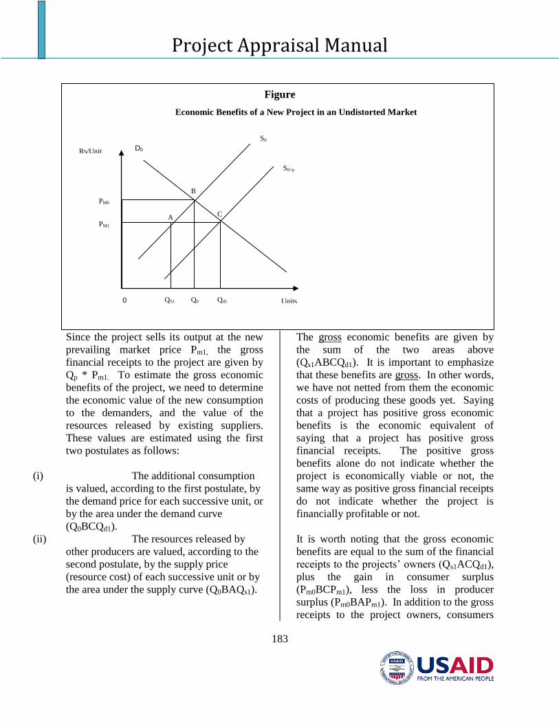
Project Appraisal Manual
183
Figure
Economic Benefits of a New Project in an Undistorted Market
Since the project sells its output at the new
prevailing market price Pm1, the gross
financial receipts to the project are given by
Qp * Pm1. To estimate the gross economic
benefits of the project, we need to determine
the economic value of the new consumption
to the demanders, and the value of the
resources released by existing suppliers.
These values are estimated using the first
two postulates as follows:
(i) The additional consumption
is valued, according to the first postulate, by
the demand price for each successive unit, or
by the area under the demand curve
(Q0BCQd1).
(ii) The resources released by
other producers are valued, according to the
second postulate, by the supply price
(resource cost) of each successive unit or by
the area under the supply curve (Q0BAQs1).
The gross economic benefits are given by
the sum of the two areas above
(Qs1ABCQd1). It is important to emphasize
that these benefits are gross. In other words,
we have not netted from them the economic
costs of producing these goods yet. Saying
that a project has positive gross economic
benefits is the economic equivalent of
saying that a project has positive gross
financial receipts. The positive gross
benefits alone do not indicate whether the
project is economically viable or not, the
same way as positive gross financial receipts
do not indicate whether the project is
financially profitable or not.
It is worth noting that the gross economic
benefits are equal to the sum of the financial
receipts to the projects’ owners (Qs1ACQd1),
plus the gain in consumer surplus
(Pm0BCPm1), less the loss in producer
surplus (Pm0BAPm1). In addition to the gross
receipts to the project owners, consumers
PM0
PM1 A
Rs/Unit
Units 0 QS1 Q0 Qd1
B
C
D0 S0
S0+p
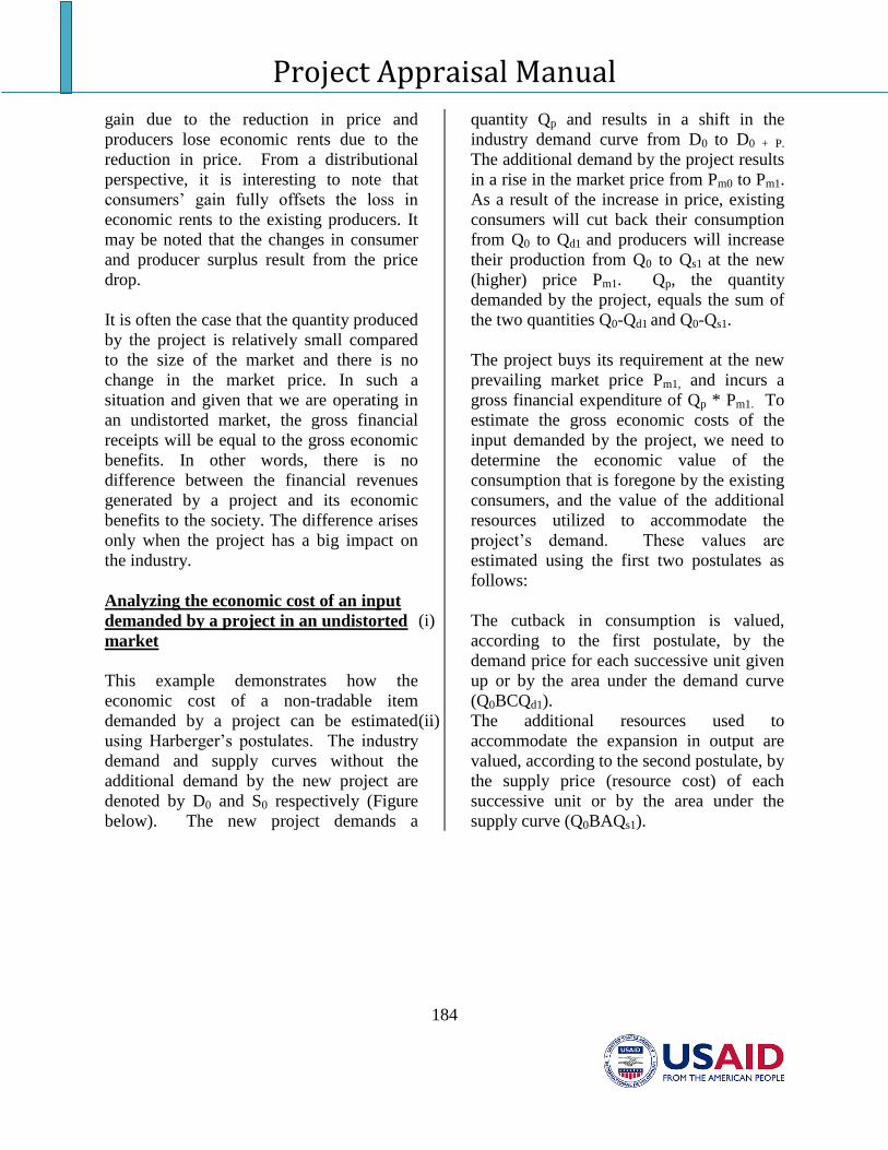
Project Appraisal Manual
184
gain due to the reduction in price and
producers lose economic rents due to the
reduction in price. From a distributional
perspective, it is interesting to note that
consumers’ gain fully offsets the loss in
economic rents to the existing producers. It
may be noted that the changes in consumer
and producer surplus result from the price
drop.
It is often the case that the quantity produced
by the project is relatively small compared
to the size of the market and there is no
change in the market price. In such a
situation and given that we are operating in
an undistorted market, the gross financial
receipts will be equal to the gross economic
benefits. In other words, there is no
difference between the financial revenues
generated by a project and its economic
benefits to the society. The difference arises
only when the project has a big impact on
the industry.
Analyzing the economic cost of an input
demanded by a project in an undistorted
market
This example demonstrates how the
economic cost of a non-tradable item
demanded by a project can be estimated
using Harberger’s postulates. The industry
demand and supply curves without the
additional demand by the new project are
denoted by D0 and S0 respectively (Figure
below). The new project demands a
quantity Qp and results in a shift in the
industry demand curve from D0 to D0 + P.
The additional demand by the project results
in a rise in the market price from Pm0 to Pm1.
As a result of the increase in price, existing
consumers will cut back their consumption
from Q0 to Qd1 and producers will increase
their production from Q0 to Qs1 at the new
(higher) price Pm1. Qp, the quantity
demanded by the project, equals the sum of
the two quantities Q0-Qd1 and Q0-Qs1.
The project buys its requirement at the new
prevailing market price Pm1, and incurs a
gross financial expenditure of Qp * Pm1. To
estimate the gross economic costs of the
input demanded by the project, we need to
determine the economic value of the
consumption that is foregone by the existing
consumers, and the value of the additional
resources utilized to accommodate the
project’s demand. These values are
estimated using the first two postulates as
follows:
(i) The cutback in consumption is valued,
according to the first postulate, by the
demand price for each successive unit given
up or by the area under the demand curve
(Q0BCQd1).
(ii) The additional resources used to
accommodate the expansion in output are
valued, according to the second postulate, by
the supply price (resource cost) of each
successive unit or by the area under the
supply curve (Q0BAQs1).
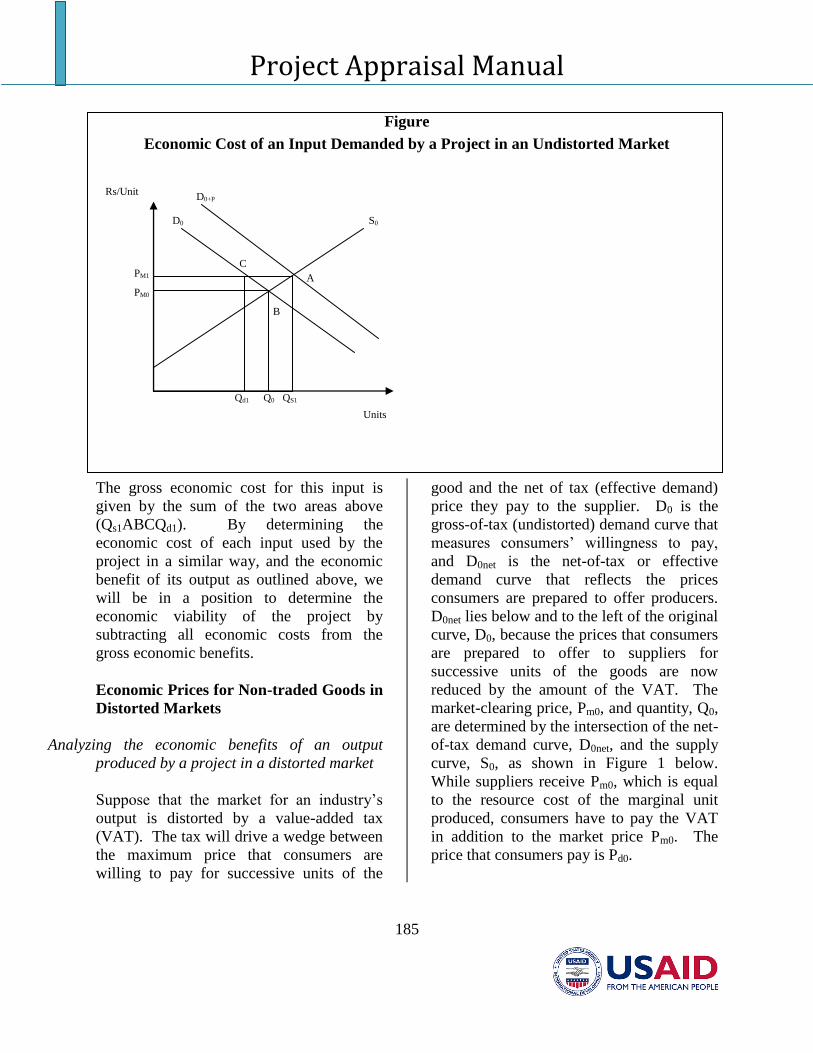
Project Appraisal Manual
185
Figure
Economic Cost of an Input Demanded by a Project in an Undistorted Market
The gross economic cost for this input is
given by the sum of the two areas above
(Qs1ABCQd1). By determining the
economic cost of each input used by the
project in a similar way, and the economic
benefit of its output as outlined above, we
will be in a position to determine the
economic viability of the project by
subtracting all economic costs from the
gross economic benefits.
Economic Prices for Non-traded Goods in
Distorted Markets
Analyzing the economic benefits of an output
produced by a project in a distorted market
Suppose that the market for an industry’s
output is distorted by a value-added tax
(VAT). The tax will drive a wedge between
the maximum price that consumers are
willing to pay for successive units of the
good and the net of tax (effective demand)
price they pay to the supplier. D0 is the
gross-of-tax (undistorted) demand curve that
measures consumers’ willingness to pay,
and D0net is the net-of-tax or effective
demand curve that reflects the prices
consumers are prepared to offer producers.
D0net lies below and to the left of the original
curve, D0, because the prices that consumers
are prepared to offer to suppliers for
successive units of the goods are now
reduced by the amount of the VAT. The
market-clearing price, Pm0, and quantity, Q0,
are determined by the intersection of the net-
of-tax demand curve, D0net, and the supply
curve, S0, as shown in Figure 1 below.
While suppliers receive Pm0, which is equal
to the resource cost of the marginal unit
produced, consumers have to pay the VAT
in addition to the market price Pm0. The
price that consumers pay is Pd0.
S0
PM1
PM0
A
B
C
Units
Rs/Unit
Qd1 QS1 Q0
D0
D0+P
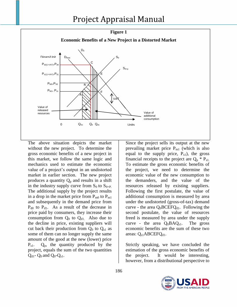
Project Appraisal Manual
186
Figure 1
Economic Benefits of a New Project in a Distorted Market
The above situation depicts the market
without the new project. To determine the
gross economic benefits of a new project in
this market, we follow the same logic and
mechanics used to estimate the economic
value of a project’s output in an undistorted
market in earlier section. The new project
produces a quantity Qp and results in a shift
in the industry supply curve from S0 to S0+P.
The additional supply by the project results
in a drop in the market price from Pm0 to Pm1
and subsequently in the demand price from
Pd0 to Pd1. As a result of the decrease in
price paid by consumers, they increase their
consumption from Q0 to Qd1. Also due to
the decline in price, existing suppliers will
cut back their production from Q0 to Qs1 as
some of them can no longer supply the same
amount of the good at the new (lower) price
Ps1. Qp, the quantity produced by the
project, equals the sum of the two quantities
Qd1- Q0 and Q0-Qs1.
Since the project sells its output at the new
prevailing market price Pm1 (which is also
equal to the supply price, Ps1), the gross
financial receipts to the project are Qp * Ps1.
To estimate the gross economic benefits of
the project, we need to determine the
economic value of the new consumption to
the demanders, and the value of the
resources released by existing suppliers.
Following the first postulate, the value of
additional consumption is measured by area
under the undistorted (gross-of-tax) demand
curve - the area Q0BCEFQd1. Following the
second postulate, the value of resources
freed is measured by area under the supply
curve - the area Q0BAQs1. The gross
economic benefits are the sum of these two
areas: Qs1ABCEFQd1.
Strictly speaking, we have concluded the
estimation of the gross economic benefits of
the project. It would be interesting,
however, from a distributional perspective to
Qd1
D0net
Ps1(1+VAT)=Pd1
Dinars/Unit
Ps0(1+VAT)=Pd0
PM0=PS0
PM1= Ps1
S0+p
E
C
A F
S0
D0
Units 0 QS1 Q0
Value of additional consumption
Value of released resources
VAT
B
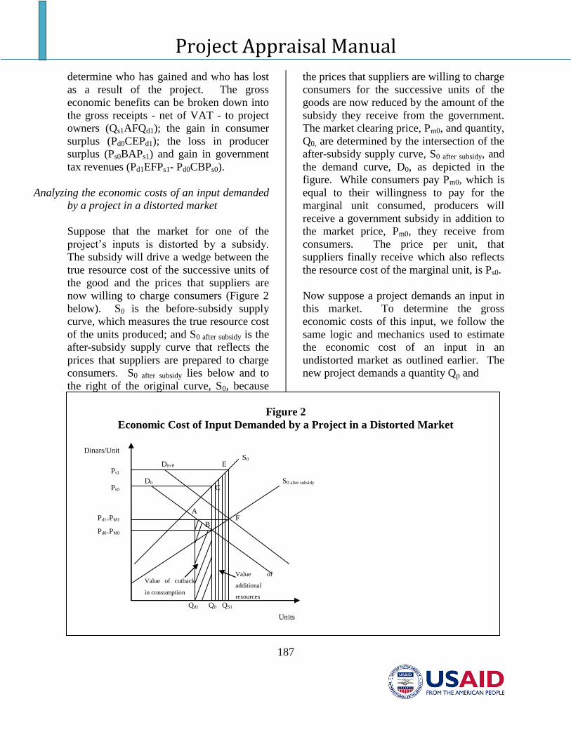
Project Appraisal Manual
187
determine who has gained and who has lost
as a result of the project. The gross
economic benefits can be broken down into
the gross receipts - net of VAT - to project
owners (Qs1AFQd1); the gain in consumer
surplus (Pd0CEPd1); the loss in producer
surplus (Ps0BAPs1) and gain in government
tax revenues (Pd1EFPs1- Pd0CBPs0).
Analyzing the economic costs of an input demanded
by a project in a distorted market
Suppose that the market for one of the
project’s inputs is distorted by a subsidy.
The subsidy will drive a wedge between the
true resource cost of the successive units of
the good and the prices that suppliers are
now willing to charge consumers (Figure 2
below). S0 is the before-subsidy supply
curve, which measures the true resource cost
of the units produced; and S0 after subsidy is the
after-subsidy supply curve that reflects the
prices that suppliers are prepared to charge
consumers. S0 after subsidy lies below and to
the right of the original curve, S0, because
the prices that suppliers are willing to charge
consumers for the successive units of the
goods are now reduced by the amount of the
subsidy they receive from the government.
The market clearing price, Pm0, and quantity,
Q0, are determined by the intersection of the
after-subsidy supply curve, S0 after subsidy, and
the demand curve, D0, as depicted in the
figure. While consumers pay Pm0, which is
equal to their willingness to pay for the
marginal unit consumed, producers will
receive a government subsidy in addition to
the market price, Pm0, they receive from
consumers. The price per unit, that
suppliers finally receive which also reflects
the resource cost of the marginal unit, is Ps0.
Now suppose a project demands an input in
this market. To determine the gross
economic costs of this input, we follow the
same logic and mechanics used to estimate
the economic cost of an input in an
undistorted market as outlined earlier. The
new project demands a quantity Qp and
Figure 2
Economic Cost of Input Demanded by a Project in a Distorted Market
Dinars/Unit S0
S0 after subsidy
Pd1=PM1
Pd0=PM0
A
C
Units
D0
D0+P
F
Ps1
Ps0
E
Value of
additional
resources
Value of cutback
in consumption
B
Qd1 QS1 Q0
Project Appraisal Manual
188
results in a shift in the industry demand
curve from D0 to D0+P. The additional
demand will bid up the market price of the
input from Pm0 to Pm1 and subsequently the
supply price from Ps0 to Ps1. The increase in
price will result in additional production by
suppliers from Q0 to Qs1, and a cutback in
consumption by the existing demanders
from Q0 to Qd1. Qp, the quantity demanded
by the project, equals the sum of the two
quantities Q0 - Qd1 and Qs1 - Q0 .
The economic cost of the project’s input is
measured by the value of the additional
resources used to accommodate the
expansion in production from Q0 to Qs1, and
the value of the cutback in consumption by
existing consumers. Following the second
postulate, the value of additional resources
used is measured by area under the before-
subsidy supply curve - the area Q0BCEFQs1.
Following the first postulate, the value of the
postponed consumption by other demanders
is measured by the area under the demand
curve - the area Q0BAQd1. The gross
economic cost is the sum of these two areas:
Qd1ABCEFQs1.
For the distributional analysis of the
project’s demand, we can breakdown the
economic costs of the input into its financial
expenditures after subsidy paid by the
project (Qd1AFQs1); the loss in consumer
surplus (Pd1ABPd0); the gain in producer
surplus (Ps0CEPs1); and the loss in
government expenditures on the subsidy
(Pd0BCPs0- Pd1FEPs1).
In the following six sections, we apply the
methodology that has been outlined above for
estimating the economic prices for non-
tradable goods and services under different
types and combinations of distortions while
illustrating each case with a numerical
example. The procedure is to start with
relatively straightforward cases for which
economic prices and conversion factors can
be easily estimated. For the more
complicated situations that ensue, the
methodology outlined below allows one to
estimate the economic prices and conversion
factors for non-tradable goods and services.
However, these more sophisticated cases also
have more demanding information
requirements.
The analyses presented here are carried out
under the assumption that despite the
distortions that might exist in the form of
taxes and subsidies, or that can be expressed
as a tax or a subsidy in the markets for these
non-tradable goods or services, there are no
quantitative restrictions on the demand for or
supply of these goods or services.34
The estimated economic prices are expressed
in terms of domestic currency.
34 For the evaluation of economic prices under
conditions of rationing, price ceilings and monopoly, see
Jenkins, Glenn P. and Arnold C. Harberger, Manual for
Cost-Benefit Analysis of Investment Decisions,
unpublished, (2005) pp. 9.14-9.24.
Project Appraisal Manual
189
Case 1: A Project Producing A Non-Tradable Output with
No Distortions in the Market for that
Output
No Distortions in any of the Factors,
Substitutes Or Complements of the
Output, and where
All Inputs Used in the Production of the
Project's Output are Non-Tradable.
When a project produces a non-tradable
output in a market where prices are
competitively set, the price of the output will,
in general, drop due to the additional supply
of the project. At the new prices, the existing
producers of the good are not willing to
supply the same quantity of the good as
before. As a result, they will cut back their
production releasing resources for alternative
uses in the economy. At the same time, the
lower prices will induce additional
consumption by the demanders of this good
or service.
If there are no distortions in the markets of the
substitutes or complements for a non-tradable
output produced by a project, and if all the
inputs used in its production are non-tradable
and their markets are undistorted, the gross
economic benefit (economic price) of the
output will be the sum of the value of the
released resources (as measured by the
competitive supply curve - area Qs1GCQ0 in
Figure 3 below and the value to the
demanders of the additional consumption as
measured by their willingness to pay - area
Q0CFQd1. In other words, the economic price
per unit of the good or service produced will
be a weighted average of the supply price per
unit (Ps) and the demand price per unit (P
d).
The supply price per unit (Ps) is the average
of the supply price before the implementation
of the project (Ps0), and the supply price after
the project (Ps1). Similarly, the demand price
per unit is the average of the demand price
before (Pd0) and after (P
d1) the
implementation of the project.
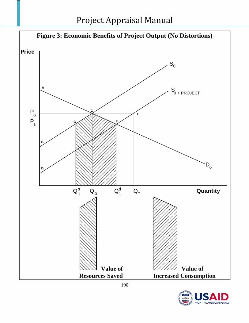
Project Appraisal Manual
190
Figure 3: Economic Benefits of Project Output (No Distortions)
S
S
1
D0
Q0
0
QT
Q1
Quantity
Price
F
B
A
C
D
G
0P
P
Q1
0 + PROJECT
E
s d
Value of Value of
Resources Saved Increased Consumption
Project Appraisal Manual
191
The weighting reflects the responsiveness of
consumers and suppliers to changes in prices of
the non-tradable output. The weight applied to
the demand side is the expected increase in the
total consumption of the good or service, as a
result of introducing the project's output,
expressed as a proportion (Wd) of the project's
sales. Similarly, the weight applied to the supply
side is the decrease in the supply by non-project
producers expressed as a proportion (Ws) of the
project's sales. The sum of these weights must
add up to one. To put it differently, it is
necessary to determine what proportion of the
quantity produced by the project replaces the
cutback in the production of the existing (non-
project) suppliers and what proportion of the
project output adds to the existing supply in the
market. Although the responsiveness and the
relative weights can be formally calculated using
elasticities, approximate values for these relative
weights are usually arrived at by applying
practical knowledge of the nature of demand and
supply in the market.35
If it is anticipated that a drop in the output price
will lead to an increase in the quantity demanded
that is roughly equal to the cutback in the
quantity supplied, then the weights can be
considered approximately equal (Ws = W
d =
0.5). Alternatively, if it is anticipated that the
35 The weight on supply (W
s) =
s / (
s -
d * (Q
d/Q
s)),
and the weight on demand (Wd) = -(
d * (Q
d/Q
s)) / (
s -
d
* (Qd/Q
s))
where: s = the price elasticity of supply
d = the price elasticity of demand
Qd = the responsive quantity
demanded in the
market without the
introduction of the
project
Qs = the responsive quantity
supplied in the
market without the
introduction of the
project.
supply response will be approximately twice the
demand response, then the weight on the supply
side of the market (Ws) will be equal to 0.67 and
that on the demand side of the market (Wd) will
be equal to 0.33.
The examples used throughout this chapter will
demonstrate how the relative weights can be
chosen for different goods and services. For
practical purposes, one can limit the choices
available to the following proportions:
1) Ws = 0.67 and W
d = 0.33
2) Ws = 0.50 and W
d = 0.50
3) Ws = 0.33 and W
d = 0.67
As subjective as the choice of these weights
might seem, the estimation of economic prices
using these weights tends to improve the
accuracy of measuring economic values as
compared to traditional approaches which place
all the weight for adjustment on either the
demand or the supply side of the market.
Estimation of Economic Prices
Algebraically, the economic price per unit of a
non-tradable output produced by a project and
expressed in the domestic currency (Pe) is
represented as follows:
Pe = W
d * P
d + W
s * P
s
where Wd + W
s = 1
When no distortions apply to the market of a
non-tradable good, the demand (Pd) and supply
price (Ps) are both equal to the market price (P
m).
In this case, if all inputs used in the production of
that good have no tradable content, the
estimation of the relative supply and demand
weights is unimportant as the economic price per
unit (Pe) is equal to the market price (P
m).
After estimating the economic price of the
output, a commodity-specific conversion factor
Project Appraisal Manual
192
(CSCF) can be obtained by dividing the
economic value per unit of output by its financial
value:
CSCFs = Economic price per unit / Financial
price per unit
This conversion factor will capture the degree of
deviation between the financial supply price of
the good and its economic price. One of the
advantages of estimating commodity-specific
conversion factors is their possible application to
other projects producing the same output.
Illustrative Example 1: A Project Providing Camp Site
Nights
Consider the competitive market for camp sites
in a beach resort where the quantities demanded
and supplied are measured in terms of camp site
nights per year. At present, and in the absence of
distortions, the quantity supplied and demanded
is 30,000 camp site nights per year at a price of
50 Dinars per night. Now introduce a project
that will provide 2,000 camp site nights per year,
and assume that the impact of the project output
on the competitive market price is small.
Let Ps = the supply price per camp site night,
Pd = the demand price per camp site night,
Pm
= the market price per camp site night,
Note that Ps = P
d = P
m = 50 Dinars.
Now consider the estimation of the economic
price per camp site night in domestic currency
generated by the project.
As the inputs used for the production of camp
site nights are largely non-tradable (land and
labor), the economic price per unit expressed at
the domestic price level (Pe) is calculated as:
Pe = W
d * P
d + W
s * P
s
Since the demand price (Pd) equals the supply
price (Ps) and each is equal to 50 Dinars
36, there
will be no need to estimate the relative demand
and supply weights; and the economic benefit
per camp site night will be equal to 50 Dinars.
Stated differently, the proportion of the project's
sales that will be a mere replacement of the
output of the non-project producers has a value
of 50 Dinars per camp site night as does the
proportion of project's sales that will lead to
increased consumption by the demanders of the
good.
The commodity-specific conversion factor for
camp site nights at the domestic price level
(CSCFs) will be equal to one as the economic
price per camp night (50 Dinars) is equal to its
financial price (50 Dinars).
36
If the quantity produced by the project is relatively large
compared to the total output of the market, it will lead to a
drop in the market price of camp site nights. When
estimating the economic price per camp site night in such
a case, we use the average of the prices without (before)
the project and those with (after) the project.
Project Appraisal Manual
193
Case 2: A Project Producing a Non-Tradable
Output Where
• Distortions Exist In The Market For That
Output,
• No Distortions In Factor, Substitute or
Complement Markets, and
• Inputs Used for the Production of the Project's
Output have Tradable Good Component.
The framework of analysis here is similar to that
used earlier to estimate the economic price of a
non-tradable output in the absence of distortions
in the output market as well as in its factor,
substitute and complement markets. The
additional supply by the project will drive the
market price of the output down, and will lead to
a cutback in production by existing producers
and an increase in consumption by demanders.
When there is a distortion in the market for the
non-tradable output of a project, the distortion
drives a wedge between the demand price, Pd,
and the supply price, Ps. Figure 4 illustrates the
effect of a project on Pd and P
s when the project's
output is subject to a sales tax. Pd0 and P
s0 are
prices without the project; Pd1 and P
s1 are prices
with the project. The gross economic benefit
(economic price) of the output will be the sum of
the value of the released resources as measured
by the supply curve of the non-project producers
- area Qs1ABQ0 in Figure 4 - and the value to the
demanders of the additional consumption as
measured by their willingness to pay - area
Q0DEQd1 in Figure 4 (following page). What the
demanders pay consists of payments to suppliers
(area Q0FCQd1) and taxes to government (area
FGEC).
Suppliers would receive Q0BCQd1 only if they
could perfectly price discriminate along the
demand curve, which is not possible in a
competitive market. However, as long as the
project’s output is small relative to the initial
market, Q0FCQd1 Q0BCQ
d1 and FGEC
BDEC.
Economic Price of a Non-Tradable Output
with Adjustment for the Foreign Exchange
Premium
In the previous case, the economic price per unit
was estimated as a weighted average of the value
of the resources saved as measured by the supply
price and value of the additional consumption as
measured by the demand price. In that situation,
it was assumed there were no distortions in the
markets for the factors used to produce the non-
tradable output and that they were all non-
tradable goods. In addition, it was assumed that
there were no distortions in the markets for the
output's complements and substitutes.
The supply price used to estimate the value of
the saved resources is based on the financial
prices of the inputs utilized in the production of
the non-tradable output. If all of these inputs are
non-tradable goods and there are no distortions
in their competitive markets, the supply price
will reflect the true economic cost to society of
the resources saved.
If there are no distortions in the markets for the
inputs used in the production of a non-tradable
output but some of these inputs are tradable
goods, then the supply price of the output will
need to be adjusted to reflect the true economic
cost of its tradable components. In this case, the
economic benefit per unit of output produced,
expressed at the domestic currency, will have
two main components. The first one is a
weighted average of the value of the released
(saved) resources measured by the competitive
supply price and the value of the additional
consumption measured by the competitive
demand price. The second component is the
premium on the foreign exchange applicable to
the tradable inputs that are now saved as the non-

Project Appraisal Manual
194
project suppliers to the market reduce their production of non-tradable output.
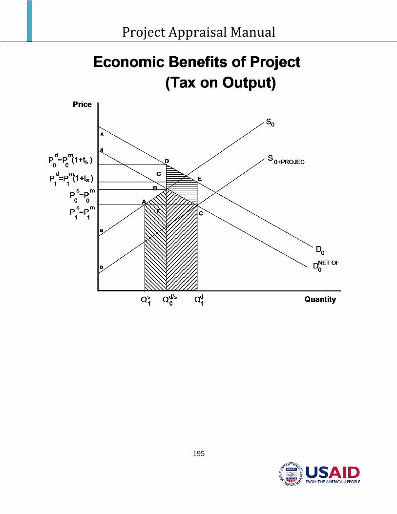
Project Appraisal Manual
195
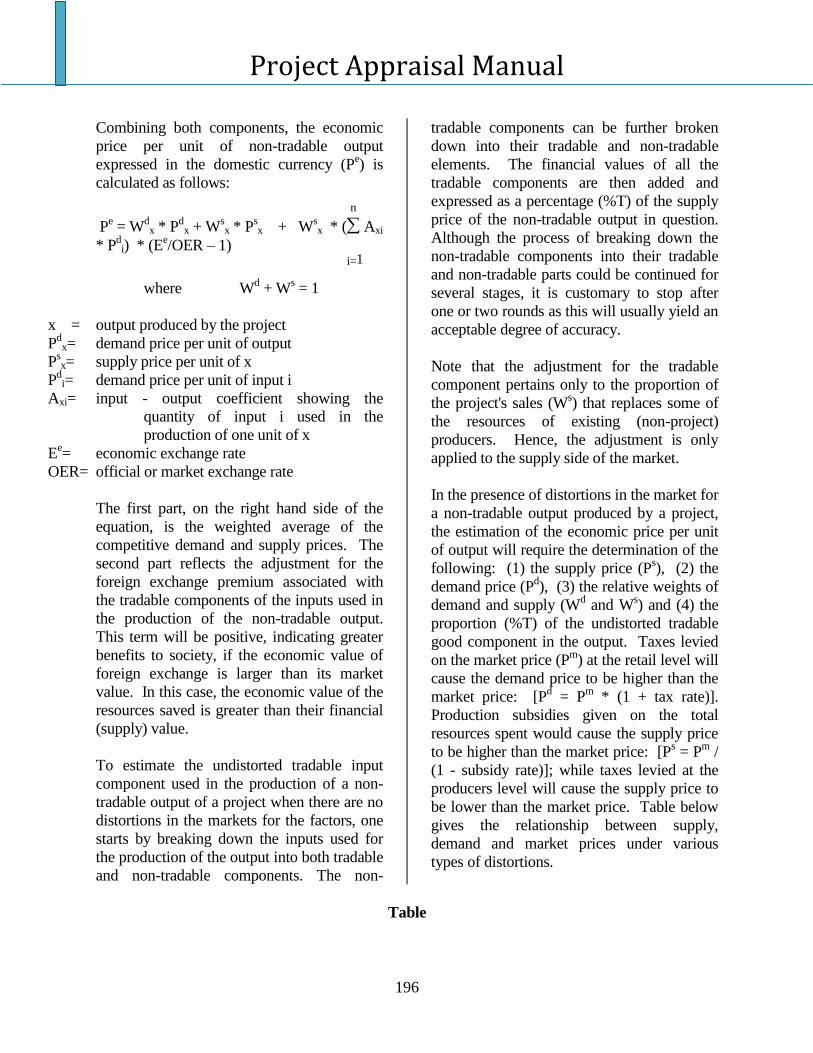
Project Appraisal Manual
196
Combining both components, the economic
price per unit of non-tradable output
expressed in the domestic currency (Pe) is
calculated as follows:
n
Pe = W
dx * P
dx + W
sx * P
sx + W
sx * ( Axi
* Pdi) * (E
e/OER – 1)
i=1
where Wd + W
s = 1
x = output produced by the project
Pdx= demand price per unit of output
Psx= supply price per unit of x
Pdi= demand price per unit of input i
Axi= input - output coefficient showing the
quantity of input i used in the
production of one unit of x
Ee= economic exchange rate
OER= official or market exchange rate
The first part, on the right hand side of the
equation, is the weighted average of the
competitive demand and supply prices. The
second part reflects the adjustment for the
foreign exchange premium associated with
the tradable components of the inputs used in
the production of the non-tradable output.
This term will be positive, indicating greater
benefits to society, if the economic value of
foreign exchange is larger than its market
value. In this case, the economic value of the
resources saved is greater than their financial
(supply) value.
To estimate the undistorted tradable input
component used in the production of a non-
tradable output of a project when there are no
distortions in the markets for the factors, one
starts by breaking down the inputs used for
the production of the output into both tradable
and non-tradable components. The non-
tradable components can be further broken
down into their tradable and non-tradable
elements. The financial values of all the
tradable components are then added and
expressed as a percentage (%T) of the supply
price of the non-tradable output in question.
Although the process of breaking down the
non-tradable components into their tradable
and non-tradable parts could be continued for
several stages, it is customary to stop after
one or two rounds as this will usually yield an
acceptable degree of accuracy.
Note that the adjustment for the tradable
component pertains only to the proportion of
the project's sales (Ws) that replaces some of
the resources of existing (non-project)
producers. Hence, the adjustment is only
applied to the supply side of the market.
In the presence of distortions in the market for
a non-tradable output produced by a project,
the estimation of the economic price per unit
of output will require the determination of the
following: (1) the supply price (Ps), (2) the
demand price (Pd), (3) the relative weights of
demand and supply (Wd and W
s) and (4) the
proportion (%T) of the undistorted tradable
good component in the output. Taxes levied
on the market price (Pm
) at the retail level will
cause the demand price to be higher than the
market price: [Pd = P
m * (1 + tax rate)].
Production subsidies given on the total
resources spent would cause the supply price
to be higher than the market price: [Ps = P
m /
(1 - subsidy rate)]; while taxes levied at the
producers level will cause the supply price to
be lower than the market price. Table below
gives the relationship between supply,
demand and market prices under various
types of distortions.
Table
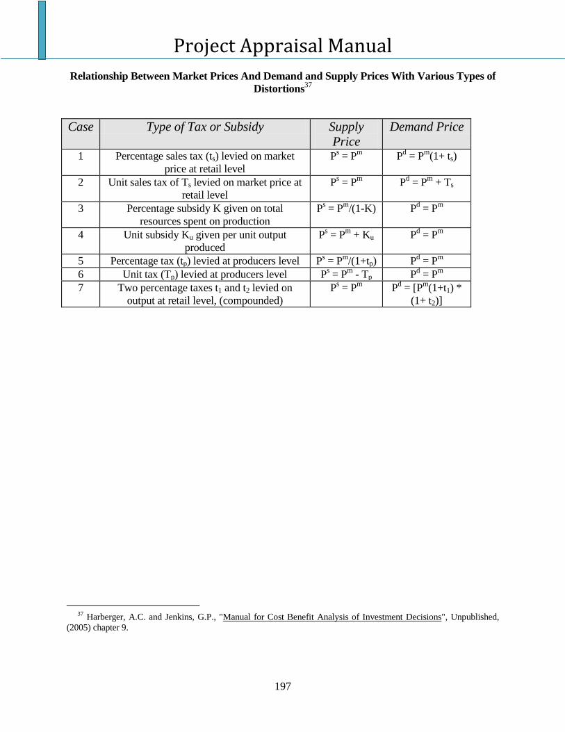
Project Appraisal Manual
197
Relationship Between Market Prices And Demand and Supply Prices With Various Types of
Distortions37
Case Type of Tax or Subsidy Supply
Price
Demand Price
1 Percentage sales tax (ts) levied on market
price at retail level
Ps = P
m P
d = P
m(1+ ts)
2 Unit sales tax of Ts levied on market price at
retail level
Ps = P
m P
d = P
m + Ts
3 Percentage subsidy K given on total
resources spent on production
Ps = P
m/(1-K) P
d = P
m
4 Unit subsidy Ku given per unit output
produced
Ps = P
m + Ku P
d = P
m
5 Percentage tax (tp) levied at producers level Ps = P
m/(1+tp) P
d = P
m
6 Unit tax (Tp) levied at producers level Ps = P
m - Tp P
d = P
m
7 Two percentage taxes t1 and t2 levied on
output at retail level, (compounded)
Ps = P
m P
d = [P
m(1+t1) *
(1+ t2)]
37
Harberger, A.C. and Jenkins, G.P., "Manual for Cost Benefit Analysis of Investment Decisions", Unpublished,
(2005) chapter 9.
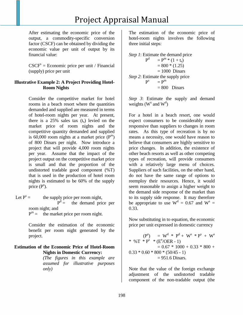
Project Appraisal Manual
198
After estimating the economic price of the
output, a commodity-specific conversion
factor (CSCF) can be obtained by dividing the
economic value per unit of output by its
financial value:
CSCFs = Economic price per unit / Financial
(supply) price per unit
Illustrative Example 2: A Project Providing Hotel-
Room Nights
Consider the competitive market for hotel
rooms in a beach resort where the quantities
demanded and supplied are measured in terms
of hotel-room nights per year. At present,
there is a 25% sales tax (ts) levied on the
market price of room nights and the
competitive quantity demanded and supplied
is 60,000 room nights at a market price (Pm
)
of 800 Dinars per night. Now introduce a
project that will provide 4,000 room nights
per year. Assume that the impact of the
project output on the competitive market price
is small and that the proportion of the
undistorted tradable good component (%T)
that is used in the production of hotel room
nights is estimated to be 60% of the supply
price (Ps).
Let Ps = the supply price per room night,
Pd = the demand price per
room night; and
Pm
= the market price per room night.
Consider the estimation of the economic
benefit per room night generated by the
project.
Estimation of the Economic Price of Hotel-Room
Nights in Domestic Currency: (The figures in this example are
assumed for illustrative purposes
only)
The estimation of the economic price of
hotel-room nights involves the following
three initial steps:
Step 1: Estimate the demand price
Pd = P
m * (1 + ts)
= 800 * (1.25)
= 1000 Dinars
Step 2: Estimate the supply price
Ps = P
m
= 800 Dinars
Step 3: Estimate the supply and demand
weights (Ws and W
d)
For a hotel in a beach resort, one would
expect consumers to be considerably more
responsive than suppliers to changes in room
rates. As this type of recreation is by no
means a necessity, one would have reason to
believe that consumers are highly sensitive to
price changes. In addition, the existence of
other beach resorts as well as other competing
types of recreation, will provide consumers
with a relatively large menu of choices.
Suppliers of such facilities, on the other hand,
do not have the same range of options to
reemploy their resources. Hence, it would
seem reasonable to assign a higher weight to
the demand side response of the market than
to its supply side response. It may therefore
be appropriate to use Wd = 0.67 and W
s =
0.33.
Now substituting in to equation, the economic
price per unit expressed in domestic currency
(Pe) = W
d * P
d + W
s * P
s + W
s
* %T * Ps * (E
e/OER - 1)
= 0.67 * 1000 + 0.33 * 800 +
0.33 * 0.60 * 800 * (50/45 - 1)
= 951.6 Dinars.
Note that the value of the foreign exchange
adjustment of the undistorted tradable
component of the non-tradable output (the
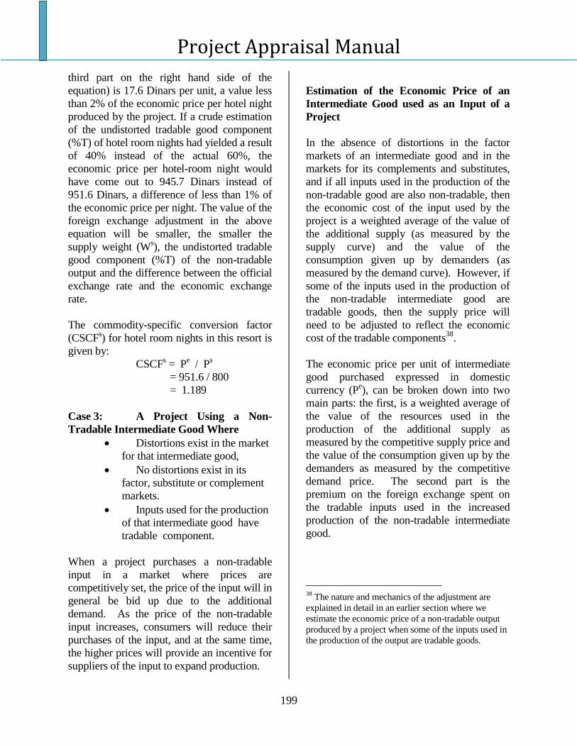
Project Appraisal Manual
199
third part on the right hand side of the
equation) is 17.6 Dinars per unit, a value less
than 2% of the economic price per hotel night
produced by the project. If a crude estimation
of the undistorted tradable good component
(%T) of hotel room nights had yielded a result
of 40% instead of the actual 60%, the
economic price per hotel-room night would
have come out to 945.7 Dinars instead of
951.6 Dinars, a difference of less than 1% of
the economic price per night. The value of the
foreign exchange adjustment in the above
equation will be smaller, the smaller the
supply weight (Ws), the undistorted tradable
good component (%T) of the non-tradable
output and the difference between the official
exchange rate and the economic exchange
rate.
The commodity-specific conversion factor
(CSCFs) for hotel room nights in this resort is
given by:
CSCFs = P
e / P
s
= 951.6 / 800
= 1.189
Case 3: A Project Using a Non-
Tradable Intermediate Good Where
Distortions exist in the market
for that intermediate good,
No distortions exist in its
factor, substitute or complement
markets.
Inputs used for the production
of that intermediate good have
tradable component.
When a project purchases a non-tradable
input in a market where prices are
competitively set, the price of the input will in
general be bid up due to the additional
demand. As the price of the non-tradable
input increases, consumers will reduce their
purchases of the input, and at the same time,
the higher prices will provide an incentive for
suppliers of the input to expand production.
Estimation of the Economic Price of an
Intermediate Good used as an Input of a
Project
In the absence of distortions in the factor
markets of an intermediate good and in the
markets for its complements and substitutes,
and if all inputs used in the production of the
non-tradable good are also non-tradable, then
the economic cost of the input used by the
project is a weighted average of the value of
the additional supply (as measured by the
supply curve) and the value of the
consumption given up by demanders (as
measured by the demand curve). However, if
some of the inputs used in the production of
the non-tradable intermediate good are
tradable goods, then the supply price will
need to be adjusted to reflect the economic
cost of the tradable components38
.
The economic price per unit of intermediate
good purchased expressed in domestic
currency (Pe), can be broken down into two
main parts: the first, is a weighted average of
the value of the resources used in the
production of the additional supply as
measured by the competitive supply price and
the value of the consumption given up by the
demanders as measured by the competitive
demand price. The second part is the
premium on the foreign exchange spent on
the tradable inputs used in the increased
production of the non-tradable intermediate
good.
38
The nature and mechanics of the adjustment are
explained in detail in an earlier section where we
estimate the economic price of a non-tradable output
produced by a project when some of the inputs used in
the production of the output are tradable goods.
Project Appraisal Manual
200
Combining both parts, the economic price per
unit of non-tradable input used by the project
and expressed at the domestic price level (Pe)
is calculated as follows:
Pe = W
dx * P
dx + W
sx * P
sx + W
sx *
%T * Psx * (E
e/OER - 1)
where W sx+ W
dx= 1
x = intermediate good purchased
by the project
%T = undistorted tradable
good component of the non-
tradable intermediate good
used by the project expressed
as a % of the financial supply
price of the intermediate good
Ee = economic exchange rate
OER = official or market exchange
rate
The first two terms on the right hand side of
the equation yield the weighted average of the
demand and supply prices. The last term
reflects the adjustment for the foreign
exchange premium attached to the undistorted
tradable components of the inputs used in the
production of the non-tradable intermediate
good. This part will be positive, indicating a
greater cost to society, if the economic value
of the foreign exchange is larger than its
market value, i.e., the economic value of the
tradable inputs is greater than their financial
value. Note that the adjustment for the
tradable component pertains only to the
proportion of the project's demand for the
intermediate good (Ws) that is met through
additional production. The proportion of the
project's demand that is accommodated
through a reduction in the purchases of other
consumers (Wd) should not be adjusted to
reflect the distortions in the input markets.
Since the production of this proportion will be
carried out regardless of whether the project is
undertaken, the adjustment is applied to only
the additional supply to this market.
In the presence of distortions in the market for
an intermediate good, the estimation of the
economic price (Pe) of the good will also
require the determination of the following:
(1) the intermediate input's supply price (Ps),
(2) its demand price (Pd), (3) the relative
weights of demand and supply (Wd and W
s)
and (4) the proportion (%T) of the undistorted
tradable good component in the costs of
production of the intermediate input.
After the estimation of the economic price of
the intermediate input, a commodity-specific
conversion factor (CSCFd) based on the
financial demand price of the input can be
calculated as follows:
CSCFd = Economic price per unit / Financial
(demand) price per unit
Illustrative Example 3: A project using bricks as an
input
Consider the competitive market for clay
bricks where at present, there is a 25% sales
tax (ts) on the market price of bricks and a
15% subsidy (K) on the suppliers' cost of
production. The quantity demanded and
supplied in the market is 7 million bricks per
month at a market price (Pm
) of 7 Dinars per
brick. Now, we introduce a project to
construct low-cost housing. During the later
stages of the construction, it is expected that
the project will require 300,000 bricks per
month. Assume that the impact of the project
demand on the competitive market price is
small and that the proportion of the
undistorted tradable good component (%T)
used in the production of bricks is estimated
to be 70% of the supply price (Ps).
Let Ps = the supply
price per brick,
Project Appraisal Manual
201
Pd = the demand
price per brick; and
Pm
= the market
price per brick.
Consider the estimation of the economic cost
of bricks in domestic currency used by this
project.
Illustration: Estimation of the Economic Price of
Bricks. (The figures in this example are
assumed for illustrative purposes
only)
Step 1: Estimate the demand price
Pdx = P
mx * (1 + ts)
= 7 * (1.25)
= 8.75 Dinars
Step 2: Estimate the supply price
Psx = P
mx / (1 - K)
= 7 / (0.85)
= 8.24 Dinars
Step 3: Estimate the supply and demand
weights
For such production activity, the expected
supply response will be small in the short run
as most brick making kilns are usually
operating close to capacity.39
Although the
supply
39
In the case of existing excess capacity, more weight
should be assigned to the supply side. As the situation
of excess capacity will likely be temporary, however,
no generalizations can be made about the economic
cost or the conversion factor of this non-tradable input.
39 The value of the foreign exchange adjustment to the
undistorted tradable component of the intermediate
good used by the project is calculated as follows:
= Ws * %T * P
s *
(Ee/OER - 1)
= 0.33 * 0.7 * 8.24 * (50/45 - 1)
= 0.21 Dinars per brick.
response will be larger in the longer run, it
will still not be as large as the demand
response. In other words, a larger proportion
of the bricks required by the project will be
obtained by existing demanders' postponing
their consumption, rather than from new
production. Hence, assigning a weight of
0.67 to the demand side and a weight of 0.33
to the supply side seems plausible.
Now substituting, the economic cost per brick
at the domestic price level (Pe)
= Wd * P
d + W
s * P
s + W
s * %T
* Ps * (E
e/OER - 1)
= 0.67 * 8.75 + 0.33 * 8.24 + 0.33 *
0.7 * 8.24 * (50 /40 - 1)
= 8.79 Dinars.
If the value of the foreign exchange
adjustment for the tradable component of the
intermediate good used by the project were to
be ignored, the economic cost per brick would
be 8.58 Dinars per unit. In other words, the
economic cost would be underestimated by
approximately 2% of the true economic cost
per brick.40
The commodity-specific conversion factor
(CSCFd) for bricks used by this project is
given by:41
CSCFd = P
e / P
d
= 8.79 / 8.75
40 Since the project uses bricks as an input, the
relevant financial price in the estimation of the
commodity-specific conversion factor is the demand
price inclusive of the 25% sales tax.
Project Appraisal Manual
202
= 1.0045
Case 4: A Project using a non-
tradable intermediate good as an input
where
Distortions exist in the market
for that intermediate good
Distortions exist in its factor
markets,
No distortions in its substitute
or complement markets
Inputs used in the production
of the intermediate good have
tradable good component.
In the previous section, a framework was
established for estimating the economic cost
of a non-tradable intermediate good where
only the market for that good was distorted.
In other words, it was assumed that the
financial prices of the inputs used in the
production of the intermediate good reflected
their economic values. This section outlines a
framework for estimating the economic cost
of an intermediate good when there are
distortions in both the market for the
intermediate good and in its factor markets.
Estimation of the economic price of an
intermediate good with distortions in both
the market for the intermediate good and
its factors markets
When distortions exist in the market for an
intermediate good, but in none of the markets
for its factors, substitutes or complements, the
economic cost per unit of that intermediate
good (Pe) is calculated as a weighted average
of the supply price (Ps) and the demand price
(Pd), plus an adjustment for the foreign
exchange premium on the tradable
components used in the production of
intermediate good.
Pe = W
dx * P
dx + W
sx * P
sx + W
sx *
%T * Psx * (E
e/OER - 1)
However, if distortions also exist in the factor
markets, an adjustment to the above equation
is required when estimating the economic cost
of the intermediate good. If, in the production
of intermediate good x, only input i is
distorted, then the economic cost per unit of
the intermediate good used by the project (Pe)
is estimated as follows:
Pe = W
dx * P
dx + W
sx * P
sx +
Wsx * %T * P
sx * (E
e/OER - 1)
- Wsx * Axi * (P
di - P
ei)
where x = intermediate good
demanded by the
project
Axi = input -output
coefficient showing
the quantity of input i
used in the production
of one unit of x
%T = undistorted tradable
good component of the
intermediate input x
expressed as a
percentage of the
financial supply price
of x
Pdx = demand price per unit
of x
Psx = supply price per unit
of x
Pdi = demand price per unit
of input i
Pei = economic value per
unit of input i
expressed in
domestic
currency.
In the case where a value-added tax (VAT) is
levied on both an intermediate good and its
Project Appraisal Manual
203
inputs, the VAT on the inputs is not
recognized as a tax because such input taxes
are allowed as a credit against the VAT on the
intermediate good. If the intermediate good is
exempt from VAT, the tax on the inputs is
treated like a sales tax because no credit is
possible at the intermediate good level. If less
than full credit is given for the input taxes,
then the excess is treated as an input tax.
Where the credit given at the intermediate
good level is greater than the underlying taxes
paid on the inputs, the excess credit is treated
as a subsidy on the purchase of the
intermediate input.
Note that any adjustments for the intermediate
good x are weighted by Wsx, the share of the
project's demand for the intermediate good x
that is met by increased supply. This
adjustment for input distortions only applies
to the additional inputs utilized because of the
increased production. The proportion of the
project's demand that is met through a
cutback in the demand of other consumers,
Wdx, is valued at the demand price P
dx and
should not be adjusted to reflect the
distortions in the input markets. This is due to
the fact that these inputs will be used in the
production of this intermediate good x
whether or not the project being considered is
implemented.
When several inputs used in the production of
the intermediate good x have distortions in
their markets, a more general form can be
used:
Pe = W
dx * P
dx + W
sx * P
sx +
Wsx * %T * P
sx * (E
e/OER - 1)
n
- Wsx * Axi * (P
di - P
ei)
i=1
In the absence of distortions in the factor
markets, the data required to estimate the
economic cost of an intermediate good x are
the supply and demand prices for the good, its
relative demand and supply weights and its
undistorted tradable good component (%T).
With distortions in the factor markets, three
additional pieces of information are required
for each distorted input i: (1) its input-output
coefficient (Axi), (2) its demand price (Pdi)
and (3) its economic price (Pei).
If the commodity-specific conversion factors
(CSCFdi) are known for all inputs that have
distortions in their markets and that are
considered in the estimation of the economic
cost of the intermediate good (Pex) the
following alternative representation of
equation can be used:42
Pex = W
dx * P
dx + W
sx * P
sx +
Wsx * %T * P
sx * (E
e/OER - 1)
n
- Wsx * {Axi * (1 - CSCF
di)*
Pdi}
i=1
The process of adjusting the economic cost of
intermediate goods for differences between
the financial (demand) prices and the
economic prices of their inputs could be
iterated back through several stages of
production. However, correcting for the
distortions in the market for an intermediate
42
Since the supply price of an intermediate good x is
based on the financial demand prices of all inputs used
in its production, one should use the demand price to
estimate the commodity-specific conversion factor
(CSCFd) for each of the inputs. Note that the
commodity-specific conversion factor calculated on
the basis of the demand price could be represented in
terms of the commodity-specific conversion factor
calculated on the basis of the supply price (CSCFs) as
follows:
CSCFd = CSCF
s * (P
s / P
d).
See Asian Development Bank, Economics Office,
"Guidelines For Economic Analysis of Projects"
(1987) page 93.
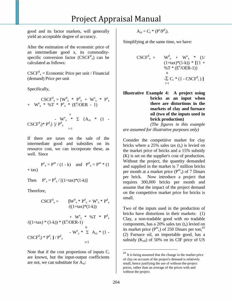
Project Appraisal Manual
204
good and its factor markets, will generally
yield an acceptable degree of accuracy.
After the estimation of the economic price of
an intermediate good x, its commodity-
specific conversion factor (CSCFdx) can be
calculated as follows:
CSCFdx = Economic Price per unit / Financial
(demand) Price per unit
Specifically,
CSCFdx = [W
dx * P
dx + W
sx * P
sx
+ Wsx * %T * P
sx * (E
e/OER - 1)
n
- Wsx * {Axi * (1 -
CSCFd
i)* Pdi} ]/ P
dx
i=1
If there are taxes on the sale of the
intermediate good and subsidies on its
resource cost, we can incorporate these, as
well. Since
Psx = P
m / (1 - k) and P
dx = P
m * (1
+ tax)
Then Psx = P
dx / [(1+tax)*(1-k)]
Therefore,
CSCFdx = [W
dx * P
dx + W
sx * P
dx
/((1+tax)*(1-k))
+ Wsx
* %T * Pdx
/((1+tax) * (1-k)) * (Ee/OER-1)
n
- Wsx * Axi * (1 -
CSCFdi) * P
di ] / P
dx
i=1
Note that if the cost proportions of inputs Ci
are known, but the input-output coefficients
are not, we can substitute for Axi:
Axi = Ci * (Ps/P
di).
Simplifying at the same time, we have:
CSCFdx = W
dx + W
sx * (1/
(1+tax)*(1-k)) * [{1 +
%T * (Ee/OER-1)}
n
- Ci * (1 - CSCFdi ) ]
i=1
Illustrative Example 4: A project using
bricks as an input when
there are distortions in the
markets of clay and furnace
oil (two of the inputs used in
brick production) (The figures in this example
are assumed for illustrative purposes only)
Consider the competitive market for clay
bricks where a 25% sales tax (ts) is levied on
the market price of bricks and a 15% subsidy
(K) is set on the supplier's cost of production.
Without the project, the quantity demanded
and supplied in the market is 7 million bricks
per month at a market price (Pm
x) of 7 Dinars
per brick. Now introduce a project that
requires 300,000 bricks per month and
assume that the impact of the project demand
on the competitive market price for bricks is
small.
Two of the inputs used in the production of
bricks have distortions in their markets: (1)
Clay, a non-tradable good with no tradable
components, has a 20% sales tax (ts) levied on
its market price (Pm
c) of 250 Dinars per ton;43
(2) Furnace oil, an importable good, has a
subsidy (Koil) of 50% on its CIF price of US
43
It is being assumed that the change in the market price
of clay on account of the project's demand is relatively
small, hence justifying the use of without-the-project
prices, rather than an average of the prices with and
without the project.
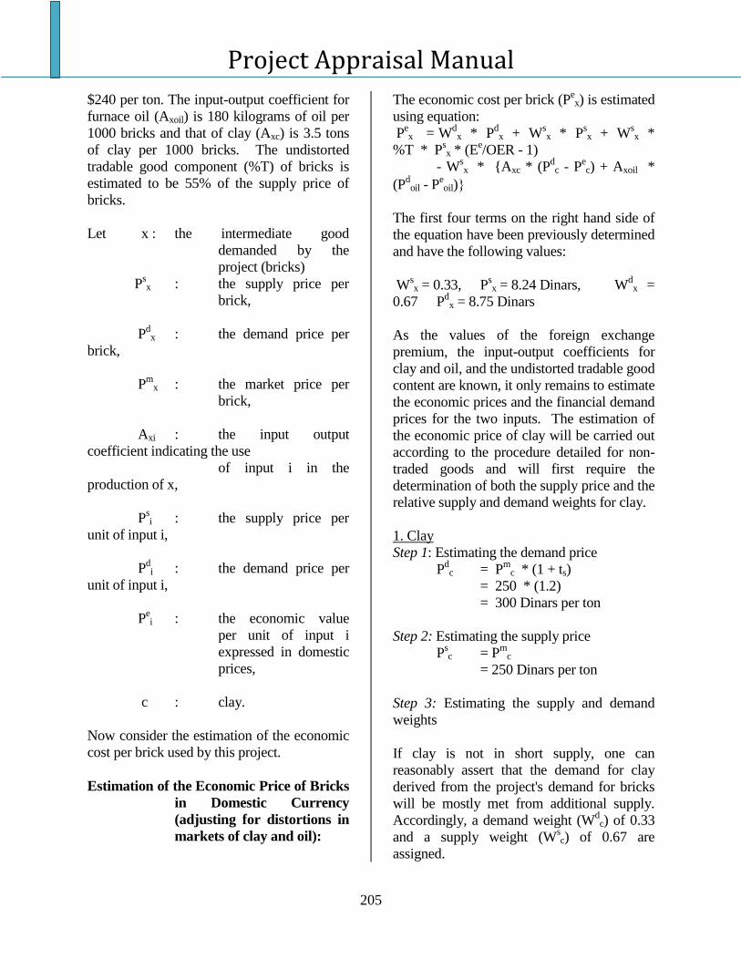
Project Appraisal Manual
205
$240 per ton. The input-output coefficient for
furnace oil (Axoil) is 180 kilograms of oil per
1000 bricks and that of clay (Axc) is 3.5 tons
of clay per 1000 bricks. The undistorted
tradable good component (%T) of bricks is
estimated to be 55% of the supply price of
bricks.
Let x : the intermediate good
demanded by the
project (bricks)
Psx : the supply price per
brick,
Pdx : the demand price per
brick,
Pm
x : the market price per
brick,
Axi : the input output
coefficient indicating the use
of input i in the
production of x,
Psi : the supply price per
unit of input i,
Pdi : the demand price per
unit of input i,
Pei : the economic value
per unit of input i
expressed in domestic
prices,
c : clay.
Now consider the estimation of the economic
cost per brick used by this project.
Estimation of the Economic Price of Bricks
in Domestic Currency
(adjusting for distortions in
markets of clay and oil):
The economic cost per brick (Pex) is estimated
using equation:
Pex = W
dx * P
dx + W
sx * P
sx + W
sx *
%T * Psx * (E
e/OER - 1)
- Wsx * {Axc * (P
dc - P
ec) + Axoil *
(Pdoil - P
eoil)
The first four terms on the right hand side of
the equation have been previously determined
and have the following values:
Wsx = 0.33, P
sx = 8.24 Dinars, W
dx =
0.67 Pdx = 8.75 Dinars
As the values of the foreign exchange
premium, the input-output coefficients for
clay and oil, and the undistorted tradable good
content are known, it only remains to estimate
the economic prices and the financial demand
prices for the two inputs. The estimation of
the economic price of clay will be carried out
according to the procedure detailed for non-
traded goods and will first require the
determination of both the supply price and the
relative supply and demand weights for clay.
1. Clay
Step 1: Estimating the demand price
Pdc = P
mc * (1 + ts)
= 250 * (1.2)
= 300 Dinars per ton
Step 2: Estimating the supply price
Psc = P
mc
= 250 Dinars per ton
Step 3: Estimating the supply and demand
weights
If clay is not in short supply, one can
reasonably assert that the demand for clay
derived from the project's demand for bricks
will be mostly met from additional supply.
Accordingly, a demand weight (Wdc) of 0.33
and a supply weight (Wsc) of 0.67 are
assigned.
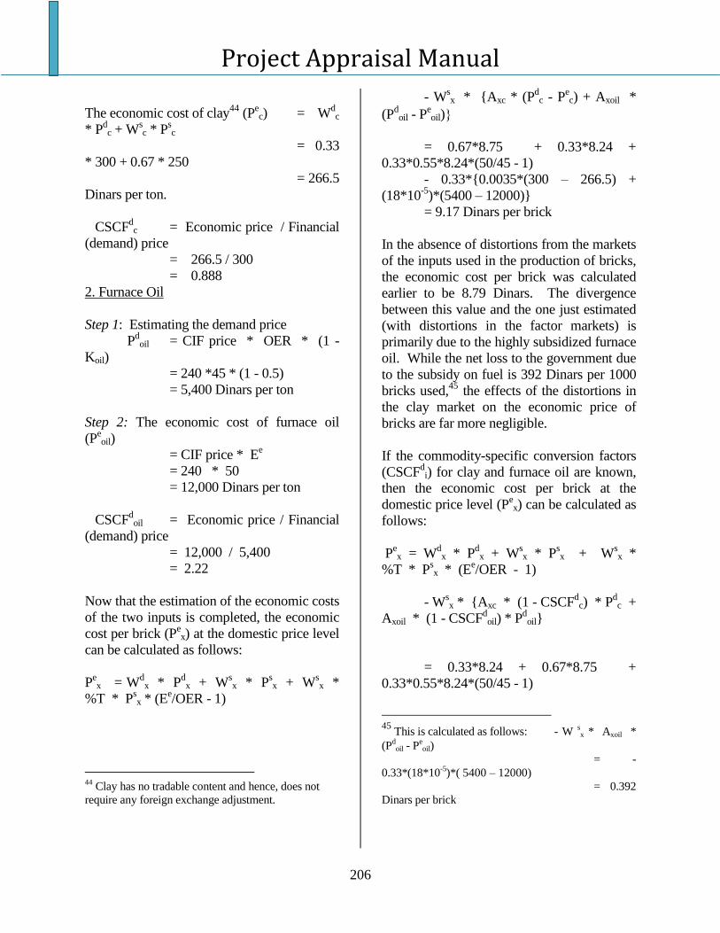
Project Appraisal Manual
206
The economic cost of clay44
(Pec) = W
dc
* Pdc + W
sc * P
sc
= 0.33
* 300 + 0.67 * 250
= 266.5
Dinars per ton.
CSCFdc = Economic price / Financial
(demand) price
= 266.5 / 300
= 0.888
2. Furnace Oil
Step 1: Estimating the demand price
Pdoil = CIF price * OER * (1 -
Koil)
= 240 *45 * (1 - 0.5)
= 5,400 Dinars per ton
Step 2: The economic cost of furnace oil
(Peoil)
= CIF price * Ee
= 240 * 50
= 12,000 Dinars per ton
CSCFdoil = Economic price / Financial
(demand) price
= 12,000 / 5,400
= 2.22
Now that the estimation of the economic costs
of the two inputs is completed, the economic
cost per brick (Pex) at the domestic price level
can be calculated as follows:
Pex = W
dx * P
dx + W
sx * P
sx + W
sx *
%T * Psx * (E
e/OER - 1)
44
Clay has no tradable content and hence, does not
require any foreign exchange adjustment.
- Wsx * {Axc * (P
dc - P
ec) + Axoil *
(Pdoil - P
eoil)
= 0.67*8.75 + 0.33*8.24 +
0.33*0.55*8.24*(50/45 - 1)
- 0.33*{0.0035*(300 – 266.5) +
(18*10-5
)*(5400 – 12000)}
= 9.17 Dinars per brick
In the absence of distortions from the markets
of the inputs used in the production of bricks,
the economic cost per brick was calculated
earlier to be 8.79 Dinars. The divergence
between this value and the one just estimated
(with distortions in the factor markets) is
primarily due to the highly subsidized furnace
oil. While the net loss to the government due
to the subsidy on fuel is 392 Dinars per 1000
bricks used,45
the effects of the distortions in
the clay market on the economic price of
bricks are far more negligible.
If the commodity-specific conversion factors
(CSCFdi) for clay and furnace oil are known,
then the economic cost per brick at the
domestic price level (Pex) can be calculated as
follows:
Pex = W
dx * P
dx + W
sx * P
sx + W
sx *
%T * Psx * (E
e/OER - 1)
- Wsx * {Axc * (1 - CSCF
dc) * P
dc +
Axoil * (1 - CSCFdoil) * P
doil}
= 0.33*8.24 + 0.67*8.75 +
0.33*0.55*8.24*(50/45 - 1)
45
This is calculated as follows: - W sx * Axoil *
(Pdoil - P
eoil)
= -
0.33*(18*10-5
)*( 5400 – 12000)
= 0.392
Dinars per brick

Project Appraisal Manual
207
- 0.33*{0.0035*(1 - 0.888)*300 +
(18*10-5
)*(1 - 2.3)*5400}
= 9.17 Dinars per brick.
The commodity-specific conversion factor
(CSCFdx) for bricks purchased by the project
is calculated as follows:
CSCFdx = P
ex / P
dx
= 9.17 / 8.75
= 1.048
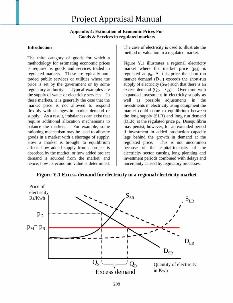
Project Appraisal Manual
208
Appendix 4: Estimation of Economic Prices For
Goods & Services in regulated markets
Introduction
The third category of goods for which a
methodology for estimating economic prices
is required is goods and services traded in
regulated markets. These are typically non-
traded public services or utilities where the
price is set by the government or by some
regulatory authority. Typical examples are
the supply of water or electricity services. In
these markets, it is generally the case that the
market price is not allowed to respond
flexibly with changes in market demand or
supply. As a result, imbalances can exist that
require additional allocation mechanisms to
balance the markets. For example, some
rationing mechanism may be used to allocate
goods in a market with a shortage of supply.
How a market is brought to equilibrium
affects how added supply from a project is
absorbed by the market, or how added project
demand is sourced from the market, and
hence, how its economic value is determined.
The case of electricity is used to illustrate the
method of valuation in a regulated market.
Figure Y.1 illustrates a regional electricity
market where the market price (pM) is
regulated at pR. At this price the short-run
market demand (DSR) exceeds the short-run
supply of electricity (SSR) such that there is an
excess demand (QD – QS). Over time with
expanded investment in electricity supply as
well as possible adjustments in the
investments in electricity using equipment the
market could come to equilibrium between
the long supply (SLR) and long run demand
(DLR) at the regulated price pR. Disequilibria
may persist, however, for an extended period
if investment in added production capacity
lags behind the growth in demand at the
regulated price. This is not uncommon
because of the capital-intensity of the
electricity sector causing long planning and
investment periods combined with delays and
uncertainty caused by regulatory processes.
Figure Y.1 Excess demand for electricity in a regional electricity market
SSR SLR
DLR
DSR
pM= pR
QS QD
Excess demand
pD
Price of
electricity
Rs/Kwh
Quantity of electricity
in Kwh
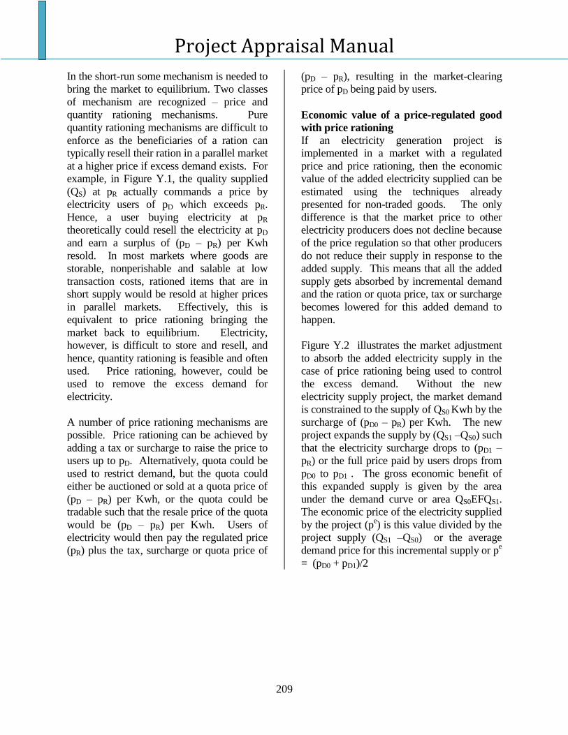
Project Appraisal Manual
209
In the short-run some mechanism is needed to
bring the market to equilibrium. Two classes
of mechanism are recognized – price and
quantity rationing mechanisms. Pure
quantity rationing mechanisms are difficult to
enforce as the beneficiaries of a ration can
typically resell their ration in a parallel market
at a higher price if excess demand exists. For
example, in Figure Y.1, the quality supplied
(QS) at pR actually commands a price by
electricity users of pD which exceeds pR.
Hence, a user buying electricity at pR
theoretically could resell the electricity at pD
and earn a surplus of (pD – pR) per Kwh
resold. In most markets where goods are
storable, nonperishable and salable at low
transaction costs, rationed items that are in
short supply would be resold at higher prices
in parallel markets. Effectively, this is
equivalent to price rationing bringing the
market back to equilibrium. Electricity,
however, is difficult to store and resell, and
hence, quantity rationing is feasible and often
used. Price rationing, however, could be
used to remove the excess demand for
electricity.
A number of price rationing mechanisms are
possible. Price rationing can be achieved by
adding a tax or surcharge to raise the price to
users up to pD. Alternatively, quota could be
used to restrict demand, but the quota could
either be auctioned or sold at a quota price of
(pD – pR) per Kwh, or the quota could be
tradable such that the resale price of the quota
would be (pD – pR) per Kwh. Users of
electricity would then pay the regulated price
(pR) plus the tax, surcharge or quota price of
(pD – pR), resulting in the market-clearing
price of pD being paid by users.
Economic value of a price-regulated good
with price rationing
If an electricity generation project is
implemented in a market with a regulated
price and price rationing, then the economic
value of the added electricity supplied can be
estimated using the techniques already
presented for non-traded goods. The only
difference is that the market price to other
electricity producers does not decline because
of the price regulation so that other producers
do not reduce their supply in response to the
added supply. This means that all the added
supply gets absorbed by incremental demand
and the ration or quota price, tax or surcharge
becomes lowered for this added demand to
happen.
Figure Y.2 illustrates the market adjustment
to absorb the added electricity supply in the
case of price rationing being used to control
the excess demand. Without the new
electricity supply project, the market demand
is constrained to the supply of QS0 Kwh by the
surcharge of (pD0 – pR) per Kwh. The new
project expands the supply by (QS1 –QS0) such
that the electricity surcharge drops to (pD1 –
pR) or the full price paid by users drops from
pD0 to pD1 . The gross economic benefit of
this expanded supply is given by the area
under the demand curve or area QS0EFQS1.
The economic price of the electricity supplied
by the project (pe) is this value divided by the
project supply (QS1 –QS0) or the average
demand price for this incremental supply or pe
= (pD0 + pD1)/2
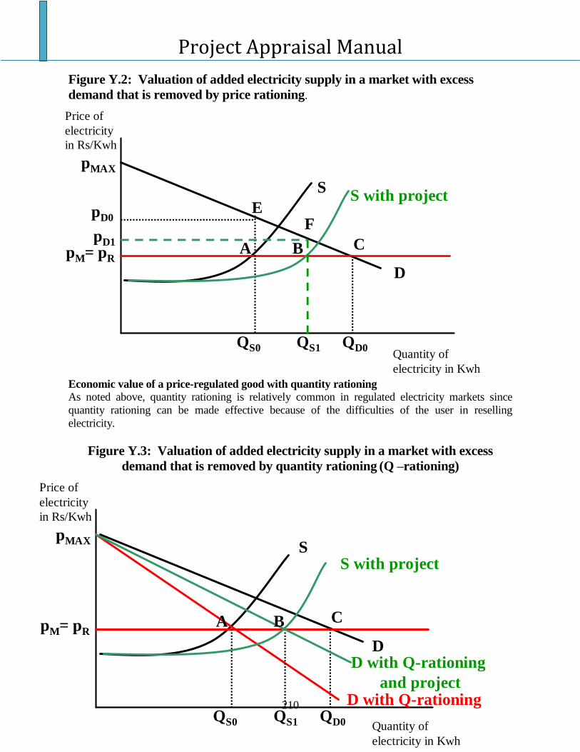
Project Appraisal Manual
210
Figure Y.2: Valuation of added electricity supply in a market with excess
demand that is removed by price rationing.
Economic value of a price-regulated good with quantity rationing As noted above, quantity rationing is relatively common in regulated electricity markets since
quantity rationing can be made effective because of the difficulties of the user in reselling
electricity.
Figure Y.3: Valuation of added electricity supply in a market with excess
demand that is removed by quantity rationing (Q –rationing)
SS with project
D
pM= pR
QS0 QD0
pMAX
QS1
A B C
pD0
pD1
EF
Price of
electricity
in Rs/Kwh
Quantity of
electricity in Kwh
SS with project
D
pM= pR
QS0 QD0
pMAX
D with Q-rationingQS1
D with Q-rationing
and project
A B C
Price of
electricity
in Rs/Kwh
Quantity of
electricity in Kwh
Project Appraisal Manual
211
Appendix 5: Evaluation of Stakeholder Impacts in Cost Benefit Analysis
Introduction
The social analysis of a project may be
organized into two parts; estimating how the
income changes caused by the project are
distributed (including the reconciliation of
financial, economic, and distributional
appraisals), and identifying the impact of the
project on the principal objectives (basic
needs) of the society. The distributional
analysis or the stakeholder analysis is the
subject of this Chapter.
The distributive analysis of the project asks
the following questions: Who will benefit
from the project and by how much? Who
will pay for the project and how much will
they pay? Project sustainability is heavily
impacted by which party in the project’s
sphere of influence gains or loses. If an
influential group is expected to bear the
burden of losses, then the successful
implementation of the project may be
hindered. The risk of a strong political
opposition to the project mobilized by the
losing party is a contingency that the project
implementers should be prepared to tackle.
Distributive Analysis
A traditional financial analysis examines the
financial feasibility of the project from the
owners’ and total investment point of view.
Economic analysis evaluates the feasibility
from the point of view of the whole country
or economy. A positive economic net
present value (NPV) implies a positive
change in the wealth of the country, while a
positive net present value from the point of
view of those with a financial interest in it,
indicates a positive expected change in the
wealth of these particular stakeholders.
The difference between the financial and
economic values of an input or output
represents a benefit or a cost that accrues to
some party other than the financial sponsors
of the project. These differences can be
analyzed by undertaking a distributive
analysis that allocates these externalities
(differences between economic and
financial) to the various parties affected. For
example, a project that causes the price of a
good to fall will create economic benefits
that are greater than its financial revenues.
This difference between the financial and
the economic values will represent a gain to
the consumers of the output and a somewhat
smaller loss to the other producers of the
good or service who are competing in the
market with the project. The differences
between the financial and economic values
of inputs and outputs also may arise due to a
variety of market distortions such as taxes
and subsidies, or because the item is sold to
consumers at a price different from the
marginal economic cost of additional
supply.
Tariffs, export taxes and subsidies, excise
and sales taxes, production subsidies and
quantitative restrictions create common
market externalities. Public goods are
normally provided at prices different than
their marginal economic costs. The
economic values of common public services
such as clean water and electricity are the
maximum amounts people are willing to pay
for these services. These values are often
significantly greater than the financial prices
people are required to pay for the services.
Any of these factors will create divergences
between the financial and the economic
prices of goods and services consumed or
produced by a project.
Project Appraisal Manual
212
A distributive analysis is composed of six
distinct steps:
Identify the externalities;
Measure the net impact of the
externalities in each market as the real
economic
values of resource flows less the real
financial values of resource flows;
Measure the values of the various
externalities throughout the life of the
project
and calculate their present values
(using the economic discount rate);
Allocate the externalities across the
various stakeholders of the project;
Summarize the distribution of the
project’s externalities and net benefits
according
to the key stakeholders in society;
Reconcile the economic and financial
resource flow statements with the
distributional impacts.
In essence, a distributive analysis seeks to
allocate the net benefits/losses generated by
a project. As a result, this analysis is
important to decision makers, as it lets them
estimate the impact of particular policies or
projects on segments of society, and to
predict which groups will be net
beneficiaries and which groups will be net
losers.
Reconciliation of Economic and Financial
Values of Inputs and Outputs
When the economic values and
corresponding financial values of variables
are expressed in terms of the same
numeraire, then we wish to show for each
variable that the economic value can be
expressed as the sum of its financial value
plus the sum of the externalities which cause
the financial and economic value to differ.
These externalities may be reflecting such
things as taxes, subsidies, changes in
consumer and producer surplus or public
good externalities.
If each of the variables are discounted using
any common discount ratio (in this case the
economic discount rate), it must also be the
case that the net present value of the
economic net benefits are equal to the net
present value of the financial net benefits,
plus the present value of the externalities.
This relationship can be expressed as in
equation (1) below:
(1) NPVee = NPV
fe +
PVe (EXTi),
where NPVee is the net present value of
economic benefits and costs, NPVef
is the
net present value of the financial benefits
and costs, and PVe (EXTi) is the sum of
the present value of all the externalities
generated by the project; all discounted
using a common rate of discount.
To indicate how this relationship holds for
non-traded and traded goods, the following
situations are considered.
The Case of a Major Expansion in the
Supply of a Non-Traded Good in an
Undistorted Market
In Figure below we illustrate the market of a
good that is the output of a project and the
market is undistorted. The project results in a
non-marginal increase in the supply of a non-
traded good in a market with no tax or
subsidy distortions. One such example
would be a project that increases the supply
of drinking water, at a lower cost, hence
expanding total consumption while also
reducing the quantity generated by higher
cost plants.
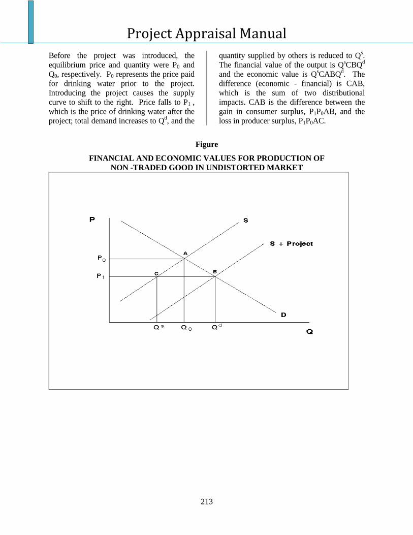
Project Appraisal Manual
213
Before the project was introduced, the
equilibrium price and quantity were P0 and
Q0, respectively. P0 represents the price paid
for drinking water prior to the project.
Introducing the project causes the supply
curve to shift to the right. Price falls to P1 ,
which is the price of drinking water after the
project; total demand increases to Qd, and the
quantity supplied by others is reduced to Qs.
The financial value of the output is QsCBQ
d
and the economic value is QsCABQ
d. The
difference (economic - financial) is CAB,
which is the sum of two distributional
impacts. CAB is the difference between the
gain in consumer surplus, P1P0AB, and the
loss in producer surplus, P1P0AC.
Figure
FINANCIAL AND ECONOMIC VALUES FOR PRODUCTION OF
NON -TRADED GOOD IN UNDISTORTED MARKET
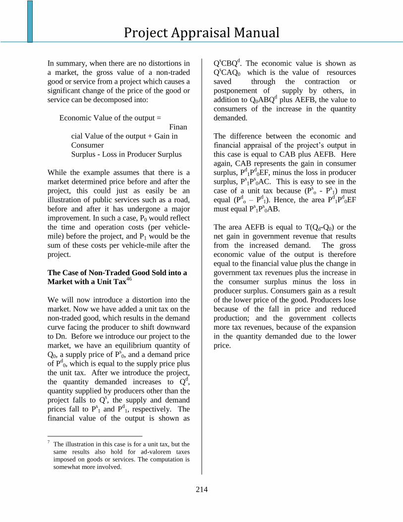
Project Appraisal Manual
214
In summary, when there are no distortions in
a market, the gross value of a non-traded
good or service from a project which causes a
significant change of the price of the good or
service can be decomposed into:
Economic Value of the output =
Finan
cial Value of the output + Gain in
Consumer
Surplus - Loss in Producer Surplus
While the example assumes that there is a
market determined price before and after the
project, this could just as easily be an
illustration of public services such as a road,
before and after it has undergone a major
improvement. In such a case, P0 would reflect
the time and operation costs (per vehicle-
mile) before the project, and P1 would be the
sum of these costs per vehicle-mile after the
project.
The Case of Non-Traded Good Sold into a
Market with a Unit Tax46
We will now introduce a distortion into the
market. Now we have added a unit tax on the
non-traded good, which results in the demand
curve facing the producer to shift downward
to Dn. Before we introduce our project to the
market, we have an equilibrium quantity of
Q0, a supply price of Ps0, and a demand price
of Pd0, which is equal to the supply price plus
the unit tax. After we introduce the project,
the quantity demanded increases to Qd,
quantity supplied by producers other than the
project falls to Qs, the supply and demand
prices fall to Ps1 and P
d1, respectively. The
financial value of the output is shown as
7
The illustration in this case is for a unit tax, but the
same results also hold for ad-valorem taxes
imposed on goods or services. The computation is
somewhat more involved.
QsCBQ
d. The economic value is shown as
QsCAQ0 which is the value of resources
saved through the contraction or
postponement of supply by others, in
addition to Q0ABQd plus AEFB, the value to
consumers of the increase in the quantity
demanded.
The difference between the economic and
financial appraisal of the project’s output in
this case is equal to CAB plus AEFB. Here
again, CAB represents the gain in consumer
surplus, Pd1P
d0EF, minus the loss in producer
surplus, Ps1P
s0AC. This is easy to see in the
case of a unit tax because (Pso - P
s1) must
equal (Pdo – P
d1). Hence, the area P
d1P
d0EF
must equal Ps1P
s0AB.
The area AEFB is equal to T(Qd-Q0) or the
net gain in government revenue that results
from the increased demand. The gross
economic value of the output is therefore
equal to the financial value plus the change in
government tax revenues plus the increase in
the consumer surplus minus the loss in
producer surplus. Consumers gain as a result
of the lower price of the good. Producers lose
because of the fall in price and reduced
production; and the government collects
more tax revenues, because of the expansion
in the quantity demanded due to the lower
price.
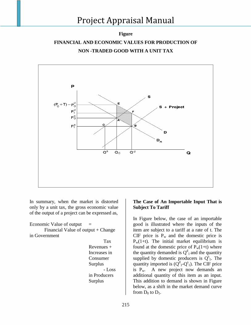
Project Appraisal Manual
215
Figure
FINANCIAL AND ECONOMIC VALUES FOR PRODUCTION OF
NON -TRADED GOOD WITH A UNIT TAX
In summary, when the market is distorted
only by a unit tax, the gross economic value
of the output of a project can be expressed as,
Economic Value of output =
Financial Value of output + Change
in Government
Tax
Revenues +
Increases in
Consumer
Surplus
- Loss
in Producers
Surplus
The Case of An Importable Input That is
Subject To Tariff
In Figure below, the case of an importable
good is illustrated where the inputs of the
item are subject to a tariff at a rate of t. The
CIF price is Pw and the domestic price is
Pw(1+t). The initial market equilibrium is
found at the domestic price of Pw(1+t) where
the quantity demanded is Qd1 and the quantity
supplied by domestic producers is Qs1. The
quantity imported is (Qd1-Q
s1). The CIF price
is Pw. A new project now demands an
additional quantity of this item as an input.
This addition to demand is shown in Figure
below, as a shift in the market demand curve
from D0 to D1.
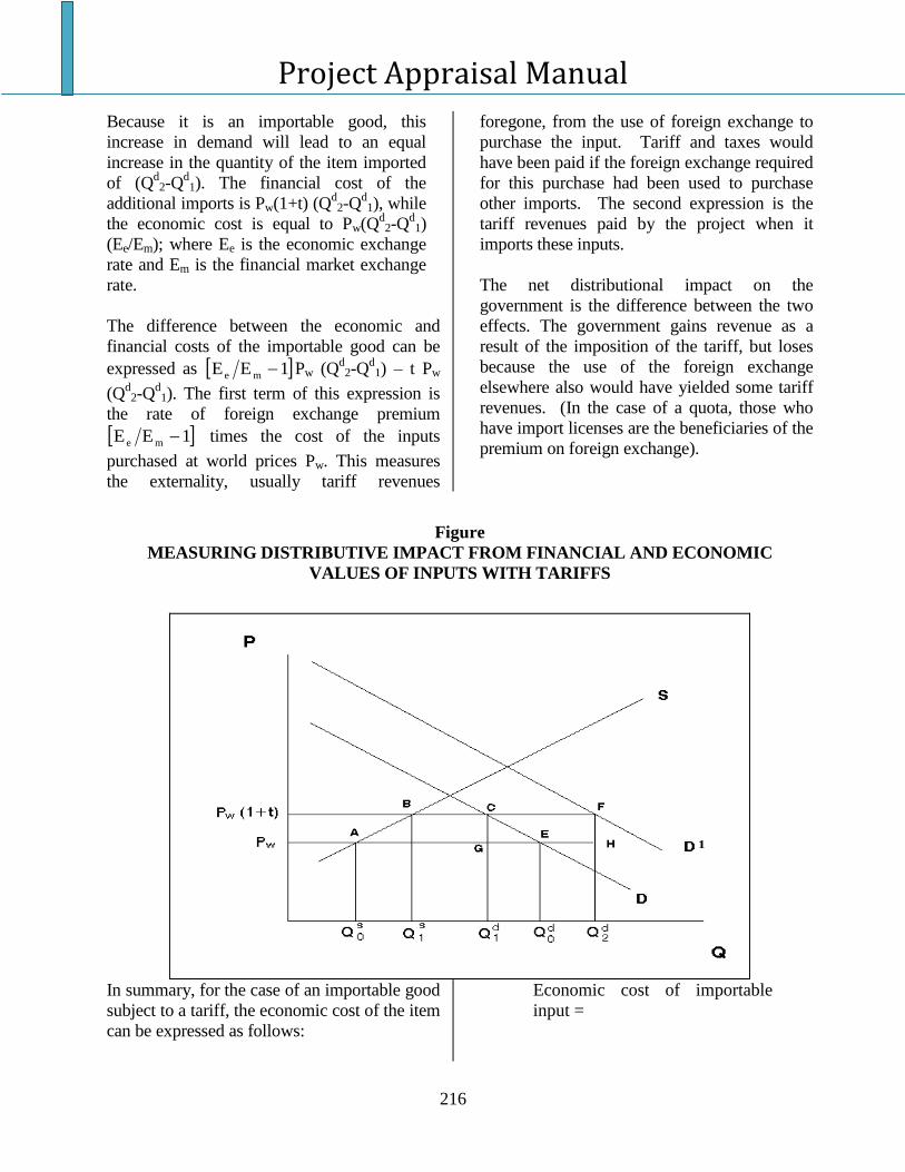
Project Appraisal Manual
216
Because it is an importable good, this
increase in demand will lead to an equal
increase in the quantity of the item imported
of (Qd2-Q
d1). The financial cost of the
additional imports is Pw(1+t) (Qd2-Q
d1), while
the economic cost is equal to Pw(Qd2-Q
d1)
(Ee/Em); where Ee is the economic exchange
rate and Em is the financial market exchange
rate.
The difference between the economic and
financial costs of the importable good can be
expressed as 1EE me Pw (Qd2-Q
d1) – t Pw
(Qd2-Q
d1). The first term of this expression is
the rate of foreign exchange premium
1EE me times the cost of the inputs
purchased at world prices Pw. This measures
the externality, usually tariff revenues
foregone, from the use of foreign exchange to
purchase the input. Tariff and taxes would
have been paid if the foreign exchange required
for this purchase had been used to purchase
other imports. The second expression is the
tariff revenues paid by the project when it
imports these inputs.
The net distributional impact on the
government is the difference between the two
effects. The government gains revenue as a
result of the imposition of the tariff, but loses
because the use of the foreign exchange
elsewhere also would have yielded some tariff
revenues. (In the case of a quota, those who
have import licenses are the beneficiaries of the
premium on foreign exchange).
Figure
MEASURING DISTRIBUTIVE IMPACT FROM FINANCIAL AND ECONOMIC
VALUES OF INPUTS WITH TARIFFS
1
In summary, for the case of an importable good
subject to a tariff, the economic cost of the item
can be expressed as follows:
Economic cost of importable
input =
Project Appraisal Manual
217
Financial cost – gain to the
government from the tariff
revenues paid on the purchase of
the item +loss in government
revenues due to the foreign
exchange premium on the foreign
exchange used to purchase this
input.
Thus, if each of the values for the input and
output variables that make up a project are
broken down into their economic, financial
and distributional components, then the end
result can be expressed as in equation (1)
where the net present value economic is equal
to the net present value of the financial
outcome of the project, plus the present value
of a series of distributional impacts on the
various stakeholders of the project.
Project Appraisal Manual
218
Appendix 6: Opportunity Cost of Foreign Exchange
Introduction
In project appraisal, there are two important
national parameters. The first national
parameter is the economic opportunity cost
of capital, which measures the economic
opportunity cost of using the capital
resources in the specific project rather than
in alternative uses in the economy. If there
are distortions in the capital markets, such as
taxes and subsidies, then there will be a
discrepancy between the financial cost of
capital that is applied to the cash flows in
the financial analysis and the economic cost
of capital that is applied to the
corresponding economic cash flows for the
investment project. The methodology to
estimate this is outlined in Appendix B.
The second national parameter is the
economic opportunity cost of foreign
exchange. Distortions in the markets that
determine the supply and demand of foreign
exchange (commonly, trade and other
indirect taxes on tradables) also result in the
economic exchange rate differing from the
financial (official or market) exchange rate.
Typically these distortions result in the
economic value of the foreign exchange
being higher than the financial value of the
foreign exchange, in which case there is a
positive foreign exchange premium. Trade
taxes and taxes on consumption (such as
sales taxes, VAT or excise duties),
importantly, tend to reduce the market
demand for imports which, in turn, reduce
the demand for foreign exchange. This
results in the strengthening in the market
exchange rate or a positive foreign exchange
premium. (The effects of tax distortions are
elaborated further below.) In the calculations
of the conversion factors for the converting
line items in the financial analysis to their
economic values, we have to take into
account the value of the foreign exchange
premium. If, for example, there are traded
inputs (or outputs) in the project, then the
value of the traded inputs (or outputs) must
be adjusted for the economic opportunity
cost of foreign exchange in the presence of
trade distortions to the extent that the use (or
production) of these traded goods results in
added demand for (or supply of) of foreign
exchange.
In some countries with controlled exchange
rates, there may be a parallel market for
foreign exchange. In the parallel market, the
“black market” exchange rate may be higher
than the official exchange rate. As a first
approximation, in the absence of any other
information, the difference between the
exchange rate in the parallel market and the
official exchange rate is probably an
underestimate of the foreign exchange
premium as it excludes the component
arising from tax and subsidy distortions.
Generally the project analyst does not have
the expertise, experience, resources or time
to conduct a reliable estimation of these
national parameters. Typically, the
appropriate government agencies will
provide guidelines or estimates for national
parameters. Ideally, for example, foreign
exchange premium estimates should be
derived from a fairly disaggregated general
equilibrium model of the economy that
captures the major distortions affecting the
foreign exchange market. However, it is
important for the project analyst to be
comfortable with the principles behind the
estimation of the two national parameters
and how they relate to the overall economic
appraisal of the investment project. For Iraq,
some rough calculations suggest that the
Project Appraisal Manual
219
foreign exchange premium is approximately
12%.47
Simple example of effect of a trade
distortion
In this section, we provide an informal
introduction to the economic opportunity
cost of foreign exchange. To illustrate the
key concepts concerning the role of trade in
the foreign exchange market, we begin with
a simple numerical example. Then we
present an informal introduction to the
underlying theoretical framework for
estimating the economic opportunity cost of
foreign exchange by examining the market
for foreign exchange.
Consider a simple case in which the only
domestic distortion on the importation of a
machine required for a project is an import
tariff of 20%. Suppose the machine costs
Iraqi Dinar 10.8 million in the domestic
market. It does not matter whether the
machine is imported or its (comparable)
equivalent is produced domestically. The
key question is whether the machine is
tradable on the world market. Also, we have
to examine the final impact of the project’s
demand for an additional unit of the
machine. In other words, it does not matter
whether our specific project imports the
machine. As explained below, what matters
is the final impact in the market for
imported machinery.
47
Rough estimates of the foreign exchange
premium (FEP) in Iraq arising from trade taxes and
other indirect consumption taxes, show that it has
dropped from around 30% in 1990 to around 20% by
the later half of the 1990s and further to around 11%
to 12% by 2004. This drop has primarily come about
with the reduction in import duties on international
trade and the major expansion in international trade
as a share of the GDP as the Iraq economy has been
opened up over the past decade. By contrast the
contribution of domestic consumption taxes to the
FEP has remained steady in the range of about 6% to
7%.
If the project imports the machine, then the
quantity of imported machines in the
economy increases by one unit. However, if
the project purchases a comparable machine
that is produced domestically, it means that
another project would not be able to
purchase that comparable machine. And
therefore, that other project would have to
import a machine. The final impact of the
demand by the project for the machine leads
to a unit increase in the number of imported
units in the economy even though our
project may not purchase an imported
machine.
Numerical example
We have assumed that the imported machine
and the machine that is produced
domestically are comparable. Consequently,
in competitive markets, the market prices for
the two machines are the same. In domestic
currency, the price of the machine is Iraqi
Dinar 10.8 million. We assume that the
foreign exchange rate is Iraqi Dinar 45/US$.
In foreign currency, the price of the machine
is US$ 240,000, inclusive of an import tariff
of 20%. The CIF price of the machine,
excluding the import tariff, is US$ 200,000.
If there were no tariff, then the price of the
machine would be the CIF price, which is
the world price. However, the tariff provides
protection to the domestic producers who
price the machines at the world price plus
the import tariff. The project has a choice.
At the same price, the project can either buy
the imported machine at the CIF price plus
the import tariff, or the domestically
produced machine.
The financial price of the machine is Iraqi
Dinar 10.8 million. The economic value of
the machine is the world price of Iraqi Dinar
9 million, exclusive of the import tariff. If
there were no tariff, then the project could
Project Appraisal Manual
220
have purchased the machine for Iraqi Dinar
9 million. Thus, the economic opportunity
cost of the machine is Iraqi Dinar 9 million,
which is the world price of the machine.
Up to this point, we have not discussed the
economic value of the foreign exchange.
The foreign exchange component of the
machine equals the value of the machine at
the world price or the amount of foreign
exchange resources the economy has to
forgo to get an additional machine.
Therefore, the incremental demand for US$
that is US$ 200,000. The import duty of
$40,000 is a transfer from the importer to
the government and is not an economic cost.
However, there may be other distortions in
the foreign exchange market, which means
that there might be a foreign exchange
premium. Assume that the foreign exchange
premium is 12%. This means that the
economic value of the foreign exchange is
higher than the CIF by 12% and the
economic value of the machine equals US$
224,000.
The details of the calculations are shown in
the table. This reviews the main concepts
just covered. The financial cost of the
machine is Iraqi Dinar 10.8 million (in
domestic currency) or US $240,000 (in
foreign currency).
Table 1: Financial and economic costs of the machine
Fin Value CF1
Econ
Val CF2
Econ
Val
Machinery, CIF, US$, '000 200.00 1.00 200.00 1.12 224.00
Import duty 40.00 0.00 0.00 0.00 0.00
Market price, US$, '000 240.00 0.833 200.00 1.12 224.00
Machinery, CIF, Iraqi Dinar
(Millions) 9.00 10.08
Import duty, Iraqi Dinar
(Millions) 1.80 0.00
Market price, Iraqi Dinar
(Millions) 10.80 10.08
Conversion factor
(intermediate) 0.833
Final conversion factor
0.833*
1,12
= 0.933
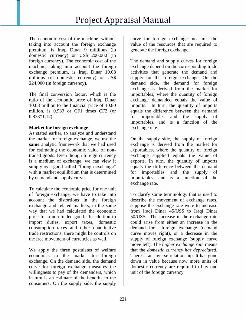
Project Appraisal Manual
221
The economic cost of the machine, without
taking into account the foreign exchange
premium, is Iraqi Dinar 9 milliions (in
domestic currency) or US$ 200,000 (in
foreign currency). The economic cost of the
machine, taking into account the foreign
exchange premium, is Iraqi Dinar 10.08
millions (in domestic currency) or US$
224,000 (in foreign currency).
The final conversion factor, which is the
ratio of the economic price of Iraqi Dinar
10.08 million to the financial price of 10.80
million, is 0.933 or CF1 times CF2 (or
0.833*1,12).
Market for foreign exchange
As stated earlier, to analyze and understand
the market for foreign exchange, we use the
same analytic framework that we had used
for estimating the economic value of non-
traded goods. Even though foreign currency
is a medium of exchange, we can view it
simply as a good called “foreign exchange”
with a market equilibrium that is determined
by demand and supply curves.
To calculate the economic price for one unit
of foreign exchange, we have to take into
account the distortions in the foreign
exchange and related markets, in the same
way that we had calculated the economic
price for a non-traded good. In addition to
import duties, export taxes, domestic
consumption taxes and other quantitative
trade restrictions, there might be controls on
the free movement of currencies as well.
We apply the three postulates of welfare
economics to the market for foreign
exchange. On the demand side, the demand
curve for foreign exchange measures the
willingness to pay of the demanders, which
in turn is an estimate of the benefits to the
consumers. On the supply side, the supply
curve for foreign exchange measures the
value of the resources that are required to
generate the foreign exchange.
The demand and supply curves for foreign
exchange depend on the corresponding trade
activities that generate the demand and
supply for the foreign exchange. On the
demand side, the demand for foreign
exchange is derived from the market for
importables, where the quantity of foreign
exchange demanded equals the value of
imports. In turn, the quantity of imports
equals the difference between the demand
for importables and the supply of
importables, and is a function of the
exchange rate.
On the supply side, the supply of foreign
exchange is derived from the market for
exportables, where the quantity of foreign
exchange supplied equals the value of
exports. In turn, the quantity of imports
equals the difference between the demand
for importables and the supply of
importables, and is a function of the
exchange rate.
To clarify some terminology that is used to
describe the movement of exchange rates,
suppose the exchange rate were to increase
from Iraqi Dinar 45/US$ to Iraqi Dinar
50/US$. The increase in the exchange rate
could arise from either an increase in the
demand for foreign exchange (demand
curve moves right), or a decrease in the
supply of foreign exchange (supply curve
move left). The higher exchange rate means
that the domestic currency has depreciated.
There is an inverse relationship. It has gone
down in value because now more units of
domestic currency are required to buy one
unit of the foreign currency.
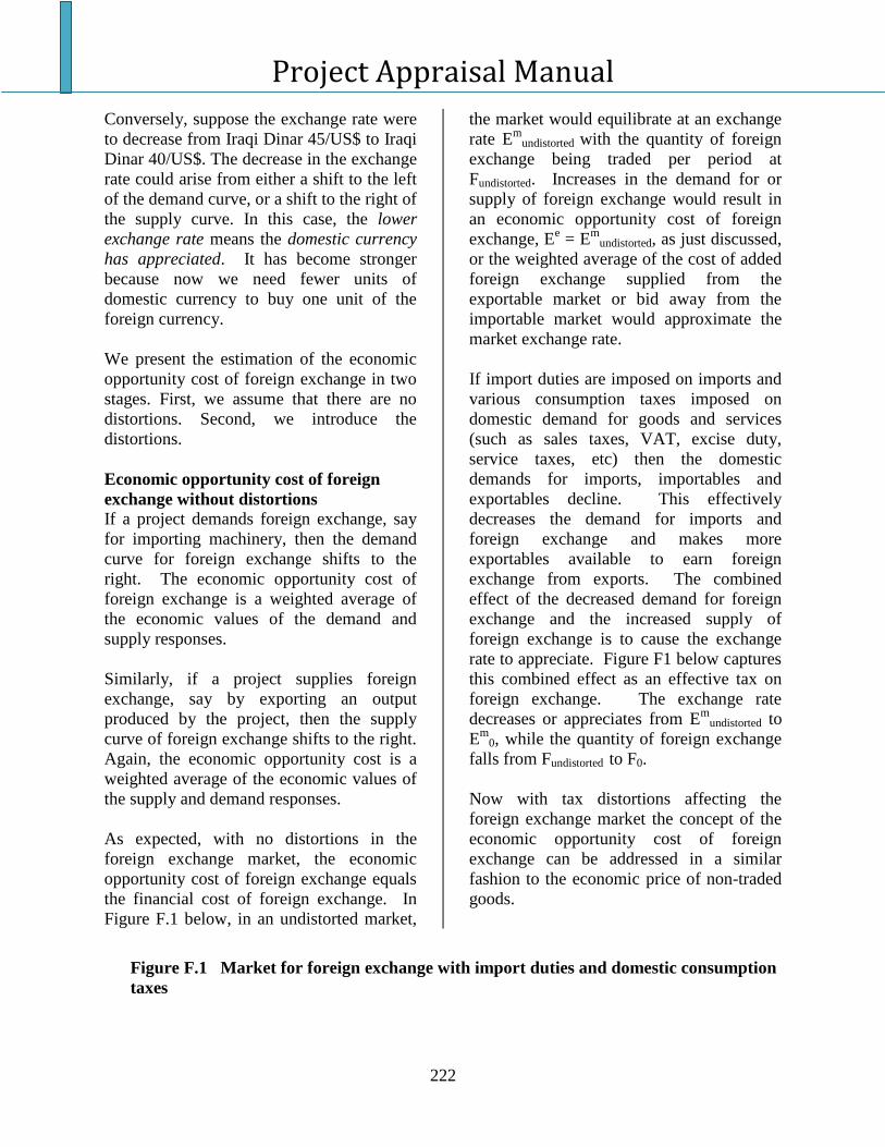
Project Appraisal Manual
222
Conversely, suppose the exchange rate were
to decrease from Iraqi Dinar 45/US$ to Iraqi
Dinar 40/US$. The decrease in the exchange
rate could arise from either a shift to the left
of the demand curve, or a shift to the right of
the supply curve. In this case, the lower
exchange rate means the domestic currency
has appreciated. It has become stronger
because now we need fewer units of
domestic currency to buy one unit of the
foreign currency.
We present the estimation of the economic
opportunity cost of foreign exchange in two
stages. First, we assume that there are no
distortions. Second, we introduce the
distortions.
Economic opportunity cost of foreign
exchange without distortions
If a project demands foreign exchange, say
for importing machinery, then the demand
curve for foreign exchange shifts to the
right. The economic opportunity cost of
foreign exchange is a weighted average of
the economic values of the demand and
supply responses.
Similarly, if a project supplies foreign
exchange, say by exporting an output
produced by the project, then the supply
curve of foreign exchange shifts to the right.
Again, the economic opportunity cost is a
weighted average of the economic values of
the supply and demand responses.
As expected, with no distortions in the
foreign exchange market, the economic
opportunity cost of foreign exchange equals
the financial cost of foreign exchange. In
Figure F.1 below, in an undistorted market,
the market would equilibrate at an exchange
rate Em
undistorted with the quantity of foreign
exchange being traded per period at
Fundistorted. Increases in the demand for or
supply of foreign exchange would result in
an economic opportunity cost of foreign
exchange, Ee = E
mundistorted, as just discussed,
or the weighted average of the cost of added
foreign exchange supplied from the
exportable market or bid away from the
importable market would approximate the
market exchange rate.
If import duties are imposed on imports and
various consumption taxes imposed on
domestic demand for goods and services
(such as sales taxes, VAT, excise duty,
service taxes, etc) then the domestic
demands for imports, importables and
exportables decline. This effectively
decreases the demand for imports and
foreign exchange and makes more
exportables available to earn foreign
exchange from exports. The combined
effect of the decreased demand for foreign
exchange and the increased supply of
foreign exchange is to cause the exchange
rate to appreciate. Figure F1 below captures
this combined effect as an effective tax on
foreign exchange. The exchange rate
decreases or appreciates from Em
undistorted to
Em
0, while the quantity of foreign exchange
falls from Fundistorted to F0.
Now with tax distortions affecting the
foreign exchange market the concept of the
economic opportunity cost of foreign
exchange can be addressed in a similar
fashion to the economic price of non-traded
goods.
Figure F.1 Market for foreign exchange with import duties and domestic consumption
taxes
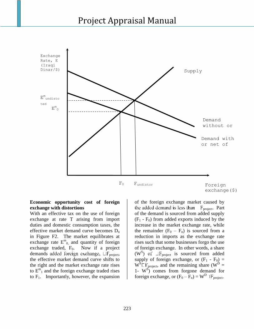
Project Appraisal Manual
223
Economic opportunity cost of foreign
exchange with distortions
With an effective tax on the use of foreign
exchange at rate T arising from import
duties and domestic consumption taxes, the
effective market demand curve becomes Dn
in Figure F2. The market equilibrates at
exchange rate Em
0, and quantity of foreign
exchange traded, F0. Now if a project
demand project,
the effective market demand curve shifts to
the right and the market exchange rate rises
to Em
1 and the foreign exchange traded rises
to F1. Importantly, however, the expansion
of the foreign exchange market caused by
project. Part
of the demand is sourced from added supply
(F1 - F0) from added exports induced by the
increase in the market exchange rate, while
the remainder (F0 – Fn) is sourced from a
reduction in imports as the exchange rate
rises such that some businesses forgo the use
of foreign exchange. In other words, a share
(WS
project is sourced from added
supply of foreign exchange, or (F1 - F0) =
WS
project, and the remaining share (WD =
1- WS) comes from forgone demand for
foreign exchange, or (F0 – Fn) = WD
project.
Supply
Demand
without or
gross of
taxes
Exchange
Rate, E
(Iraqi
Dinar/$)
Demand with
or net of
taxes
Emundisto
ted
Em0
Fundistor
ted
F0 Foreign
exchange($)
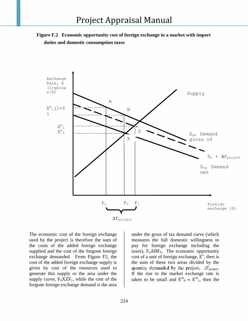
Project Appraisal Manual
224
Figure F.2 Economic opportunity cost of foreign exchange in a market with import
duties and domestic consumption taxes
The economic cost of the foreign exchange
used by the project is therefore the sum of
the costs of the added foreign exchange
supplied and the cost of the forgone foreign
exchange demanded. From Figure F2, the
cost of the added foreign exchange supply is
given by cost of the resources used to
generate this supply or the area under the
supply curve, F0XZF1, while the cost of the
forgone foreign exchange demand is the area
under the gross of tax demand curve (which
measures the full domestic willingness to
pay for foreign exchange including the
taxes), FnABF0. The economic opportunity
cost of a unit of foreign exchange, Ee, then is
the sum of these two areas divided by the
project.
If the rise in the market exchange rate is
taken to be small and Em
0 Em
1, then the
Supply
Dg, Demand
gross of
taxes
Exchange
Rate, E
(IrqDina
r/$)
Dn, Demand
net
of taxes
Em1
Em0
F0 Foreign
exchange ($)
Dn + Fproject
Em1(1+T
)
Em0(1+T
)
F1
Fproject
A
A
Fn
A
B
X
Z
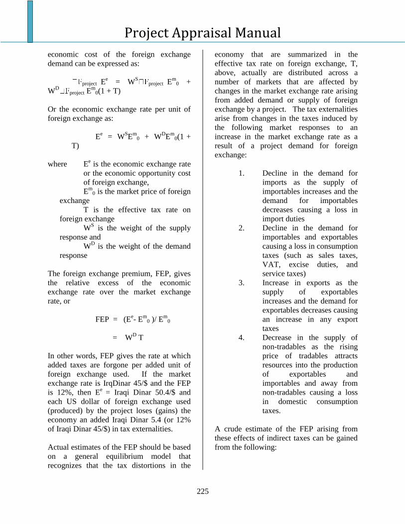
Project Appraisal Manual
225
economic cost of the foreign exchange
demand can be expressed as:
project Ee = W
Sproject E
m0 +
WD
project Em
0(1 + T)
Or the economic exchange rate per unit of
foreign exchange as:
Ee = W
SE
m0 + W
DE
m0(1 +
T)
where Ee is the economic exchange rate
or the economic opportunity cost
of foreign exchange,
Em
0 is the market price of foreign
exchange
T is the effective tax rate on
foreign exchange
WS is the weight of the supply
response and
WD is the weight of the demand
response
The foreign exchange premium, FEP, gives
the relative excess of the economic
exchange rate over the market exchange
rate, or
FEP = (Ee- E
m0 )/ E
m0
= WD T
In other words, FEP gives the rate at which
added taxes are forgone per added unit of
foreign exchange used. If the market
exchange rate is IrqDinar 45/$ and the FEP
is 12%, then Ee
= Iraqi Dinar 50.4/$ and
each US dollar of foreign exchange used
(produced) by the project loses (gains) the
economy an added Iraqi Dinar 5.4 (or 12%
of Iraqi Dinar 45/$) in tax externalities.
Actual estimates of the FEP should be based
on a general equilibrium model that
recognizes that the tax distortions in the
economy that are summarized in the
effective tax rate on foreign exchange, T,
above, actually are distributed across a
number of markets that are affected by
changes in the market exchange rate arising
from added demand or supply of foreign
exchange by a project. The tax externalities
arise from changes in the taxes induced by
the following market responses to an
increase in the market exchange rate as a
result of a project demand for foreign
exchange:
1. Decline in the demand for
imports as the supply of
importables increases and the
demand for importables
decreases causing a loss in
import duties
2. Decline in the demand for
importables and exportables
causing a loss in consumption
taxes (such as sales taxes,
VAT, excise duties, and
service taxes)
3. Increase in exports as the
supply of exportables
increases and the demand for
exportables decreases causing
an increase in any export
taxes
4. Decrease in the supply of
non-tradables as the rising
price of tradables attracts
resources into the production
of exportables and
importables and away from
non-tradables causing a loss
in domestic consumption
taxes.
A crude estimate of the FEP arising from
these effects of indirect taxes can be gained
from the following:
Project Appraisal Manual
226
FEP = M/(M+X).Tm + (0.3Tm +
0.75)V
Where: M = Value of imports of
goods and services
X = Value of exports of
goods and services
Tm = Effective import duty
rate, or import duties
over import value of
goods and services
V = Effective domestic
consumption tax rate,
or domestic
consumption taxes
over final demand
Based on revenue and macro-economic data
for Iraq through 2004, FEP is approximately
12%.
Project Appraisal Manual
227
Appendix 7: Economic Discount Rate
Why is the Economic Cost of Capital
Important?
Project appraisal requires a comparison of
the costs and benefits of a project over its
life. For acceptance, the present value of the
project's benefits should exceed the present
value of its costs. In the case of mutually
exclusive projects, its net present value
(NPV) also should be greater than those of
the alternative projects.48
The economic
opportunity cost of capital is also an
important parameter for taking decisions
relating to the optimum size of the project
and the appropriate timing for making an
investment. Both are critical factors
affecting the net benefits and the project’s
ultimate viability. In addition, the choice of
technology for a project is influenced by the
opportunity cost of capital. A low cost of
capital will encourage the use of capital-
intensive technologies as opposed to labor-
or fuel- intensive technologies. In the case of
Iraq, the situation may be the other way
around, where the cost of capital can be
high, and therefore labor intensive
technology should be encouraged.
(i) Opportunity Cost of Capital and
Investment Criteria
When the net present value (NPV) is used as
an investment criterion, it is the net benefits,
which occur over time that must be
compared for alternative projects. As the
resources available today may be used for
investments, yielding positive returns, or
alternatively may provide goods and
alternative services for immediate
consumption, it is necessary to give a greater
importance to benefits and costs that accrue
48
M. Roemer and J.J Stern, The Appraisal of
Development Projects, (New York: Praeger
Publisher, Inc., 1975).
earlier and a lower weight to those that
accrue in later periods.
In applying the NPV criterion in economic
analysis, the values of net benefits should be
discounted to a common point in time before
comparison. This is done using the
economic opportunity cost of capital as the
discount rate. When this discount rate is
used, a positive net present value means that
the project in question has a greater
economic return than would otherwise be
produced by the standard alternative use of
the same funds.
(ii) Choosing the Scale of a Project
An important decision in project appraisal
concerns the size or scale at which a facility
should be built. It is seldom that the scale of
a project is constrained by technological
factors, and economic considerations should
be paramount in selecting its appropriate
scale. Even if the project is not built to its
correct size, it may be a viable project, i.e.
its NPV may still be positive, but less than
its potential. The NPV is maximized only
when the optimum scale is chosen.
The appropriate principle to use for
determining the scale of a project is to treat
each incremental change in size as a project
in itself. An increase in the scale of a
project will require additional expenditures
and will generate additional benefits. The
net present value of the costs and benefits of
each incremental change should be
calculated by using the economic discount
rate.
The NPV of each incremental project
indicates by how much it increases or
decreases the overall net present value of the
project. This procedure is repeated until a
scale is reached where the net present value
Project Appraisal Manual
228
of incremental benefits and costs associated
with a change in scale changes from positive
to negative. When this occurs, the previous
scale is the optimum size of the plant. Thus,
the economic opportunity cost of capital or
economic discount rate is central to the
selection of the optimum scale of a project.
(iii) Timing of Investment
Another important decision to be made in
project analysis relates to the appropriate
time for a project to start. A project that is
built too soon could result in a large amount
of idle capacity. In this case, the forgone
return from the use of funds elsewhere
might be larger than the benefits gained in
the first few years of the project's life. On
the other hand, if the project is delayed too
long, shortages may occur and the forgone
benefits of the project will be greater than
the alternative yields of the invested funds.
Whenever the project is undertaken too early
or too late, its net present value will be
lower than what it could have been if
developed at the right time. The net present
value may still be positive, but it will not be
at the project's potential maximum.
The key to making a decision on this issue is
whether the costs of postponement of the
project are greater or smaller than the
benefits of postponement. For example, in a
situation where a project’s potential benefits,
net of operating costs, are growing as a
function of calendar time but its real
investment costs are the same, irrespective
of the date of initiation of the project, the
costs of postponement from year t to year
t+1 are the economic benefits Bt+1 forgone
by delaying the project. The benefit of
postponement is the economic return (re)
that can be earned from the capital invested
in its alternative use. Thus the benefit from
postponement is equal to the economic
opportunity cost of capital multiplied by the
capital costs, re Kt.
A value for the economic opportunity cost
of funds is essential in choosing the correct
time for starting the project.
(iv) Choice of Technology
In order to be worth doing, a public sector
project must have a rate of benefit of yield
that is at least as large as the economic
opportunity cost of capital. If this is not so,
the capital would better be left to be
allocated to other uses through the normal
working of the capital market.
Sometimes public sector projects face a
financial cost of capital that is artificially
low. This may happen when they can raise
debt capital at an artificially low rate of
interest because of government subsidies or
guarantees. Alternatively, public sector
projects may receive tax concessions from
the government. In either case, the cost of
capital perceived by the project will be
below its economic opportunity cost.
The use of a lower financial cost of capital
instead of its economic opportunity cost
would create an incentive for the project
managers to use production techniques that
are too capital intensive, which may not be
beneficial for the Iraqi states. The choice of
an excessively capital-intensive technology
would also lead to economic inefficiency
because the value of the marginal product of
capital in this activity is below the economic
cost of capital to the country. For example,
in electricity generation, using a financial
cost of capital that is lower than its social
cost will make capital-intensive options such
as distant hydroelectric dams or nuclear
power plants more attractive than oil- or
coal-fired generation plants. A correct
measure of the economic opportunity cost of
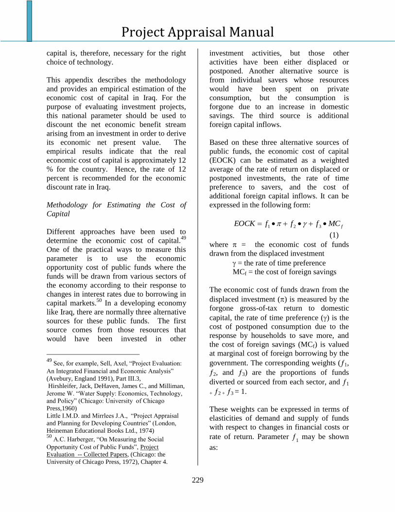
Project Appraisal Manual
229
capital is, therefore, necessary for the right
choice of technology.
This appendix describes the methodology
and provides an empirical estimation of the
economic cost of capital in Iraq. For the
purpose of evaluating investment projects,
this national parameter should be used to
discount the net economic benefit stream
arising from an investment in order to derive
its economic net present value. The
empirical results indicate that the real
economic cost of capital is approximately 12
% for the country. Hence, the rate of 12
percent is recommended for the economic
discount rate in Iraq.
Methodology for Estimating the Cost of
Capital
Different approaches have been used to
determine the economic cost of capital.49
One of the practical ways to measure this
parameter is to use the economic
opportunity cost of public funds where the
funds will be drawn from various sectors of
the economy according to their response to
changes in interest rates due to borrowing in
capital markets.50
In a developing economy
like Iraq, there are normally three alternative
sources for these public funds. The first
source comes from those resources that
would have been invested in other
49
See, for example, Sell, Axel, “Project Evaluation:
An Integrated Financial and Economic Analysis”
(Avebury, England 1991), Part III.3,
Hirshleifer, Jack, DeHaven, James C., and Milliman,
Jerome W. “Water Supply: Economics, Technology,
and Policy” (Chicago: University of Chicago
Press,1960)
Little I.M.D. and Mirrlees J.A., “Project Appraisal
and Planning for Developing Countries” (London,
Heineman Educational Books Ltd., 1974) 50
A.C. Harberger, “On Measuring the Social
Opportunity Cost of Public Funds”, Project
Evaluation -- Collected Papers, (Chicago: the
University of Chicago Press, 1972), Chapter 4.
investment activities, but those other
activities have been either displaced or
postponed. Another alternative source is
from individual savers whose resources
would have been spent on private
consumption, but the consumption is
forgone due to an increase in domestic
savings. The third source is additional
foreign capital inflows.
Based on these three alternative sources of
public funds, the economic cost of capital
(EOCK) can be estimated as a weighted
average of the rate of return on displaced or
postponed investments, the rate of time
preference to savers, and the cost of
additional foreign capital inflows. It can be
expressed in the following form:
fMCfffEOCK 321
(1)
where = the economic cost of funds
drawn from the displaced investment
= the rate of time preference
MCf = the cost of foreign savings
The economic cost of funds drawn from the
displaced investment () is measured by the
forgone gross-of-tax return to domestic
capital, the rate of time preference () is the
cost of postponed consumption due to the
response by households to save more, and
the cost of foreign savings (MCf) is valued
at marginal cost of foreign borrowing by the
government. The corresponding weights (1,
2, and 3) are the proportions of funds
diverted or sourced from each sector, and 1
+ 2 + 3 = 1.
These weights can be expressed in terms of
elasticities of demand and supply of funds
with respect to changes in financial costs or
rate of return. Parameter 1 may be shown
as:
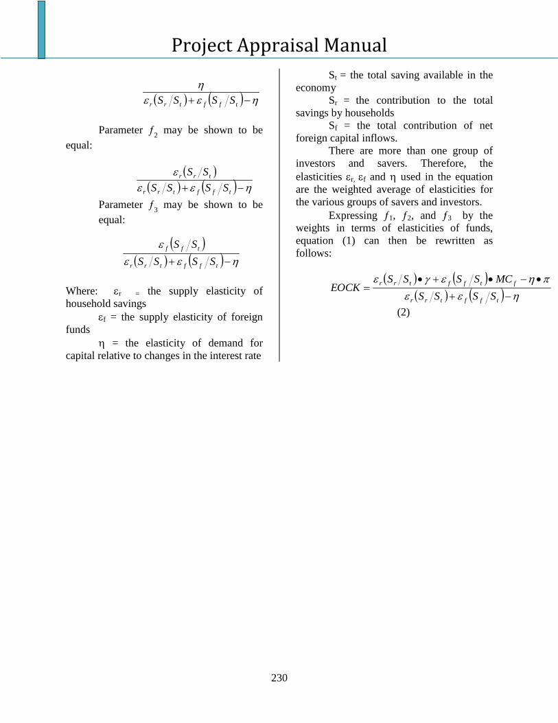
Project Appraisal Manual
230
Parameter 2 may be shown to be
equal:
Parameter 3 may be shown to be
equal:
Where: r = the supply elasticity of
household savings
f = the supply elasticity of foreign
funds
= the elasticity of demand for
capital relative to changes in the interest rate
St = the total saving available in the
economy
Sr = the contribution to the total
savings by households
Sf = the total contribution of net
foreign capital inflows.
There are more than one group of
investors and savers. Therefore, the
elasticities r, f and used in the equation
are the weighted average of elasticities for
the various groups of savers and investors. Expressing 1, 2, and 3 by the
weights in terms of elasticities of funds,
equation (1) can then be rewritten as
follows:
tfftrr
ftfftrr
SSSS
MCSSSSEOCK
(2)
tfftrr
trr
SSSS
SS
tfftrr
tff
SSSS
SS
tfftrr SSSS
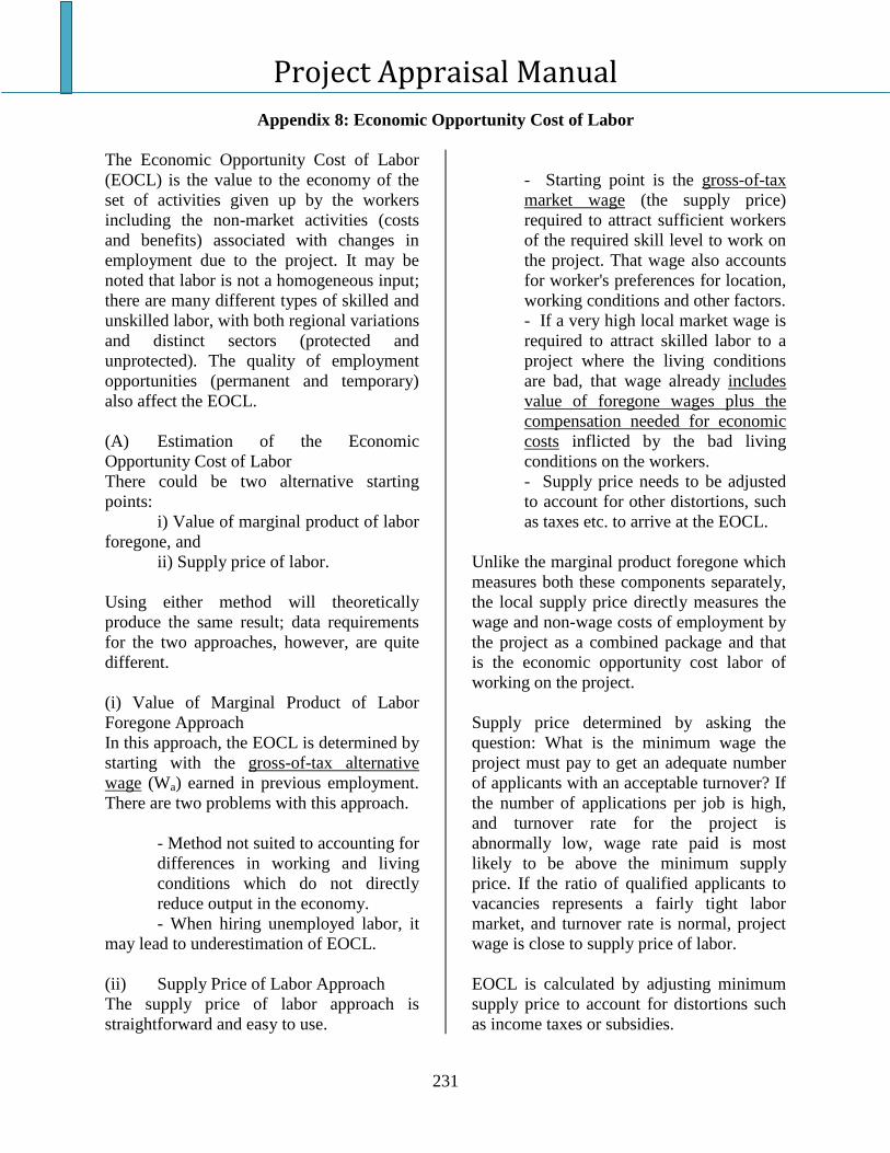
Project Appraisal Manual
231
Appendix 8: Economic Opportunity Cost of Labor
The Economic Opportunity Cost of Labor
(EOCL) is the value to the economy of the
set of activities given up by the workers
including the non-market activities (costs
and benefits) associated with changes in
employment due to the project. It may be
noted that labor is not a homogeneous input;
there are many different types of skilled and
unskilled labor, with both regional variations
and distinct sectors (protected and
unprotected). The quality of employment
opportunities (permanent and temporary)
also affect the EOCL.
(A) Estimation of the Economic
Opportunity Cost of Labor
There could be two alternative starting
points:
i) Value of marginal product of labor
foregone, and
ii) Supply price of labor.
Using either method will theoretically
produce the same result; data requirements
for the two approaches, however, are quite
different.
(i) Value of Marginal Product of Labor
Foregone Approach
In this approach, the EOCL is determined by
starting with the gross-of-tax alternative
wage (Wa) earned in previous employment.
There are two problems with this approach.
- Method not suited to accounting for
differences in working and living
conditions which do not directly
reduce output in the economy.
- When hiring unemployed labor, it
may lead to underestimation of EOCL.
(ii) Supply Price of Labor Approach
The supply price of labor approach is
straightforward and easy to use.
- Starting point is the gross-of-tax
market wage (the supply price)
required to attract sufficient workers
of the required skill level to work on
the project. That wage also accounts
for worker's preferences for location,
working conditions and other factors.
- If a very high local market wage is
required to attract skilled labor to a
project where the living conditions
are bad, that wage already includes
value of foregone wages plus the
compensation needed for economic
costs inflicted by the bad living
conditions on the workers.
- Supply price needs to be adjusted
to account for other distortions, such
as taxes etc. to arrive at the EOCL.
Unlike the marginal product foregone which
measures both these components separately,
the local supply price directly measures the
wage and non-wage costs of employment by
the project as a combined package and that
is the economic opportunity cost labor of
working on the project.
Supply price determined by asking the
question: What is the minimum wage the
project must pay to get an adequate number
of applicants with an acceptable turnover? If
the number of applications per job is high,
and turnover rate for the project is
abnormally low, wage rate paid is most
likely to be above the minimum supply
price. If the ratio of qualified applicants to
vacancies represents a fairly tight labor
market, and turnover rate is normal, project
wage is close to supply price of labor.
EOCL is calculated by adjusting minimum
supply price to account for distortions such
as income taxes or subsidies.
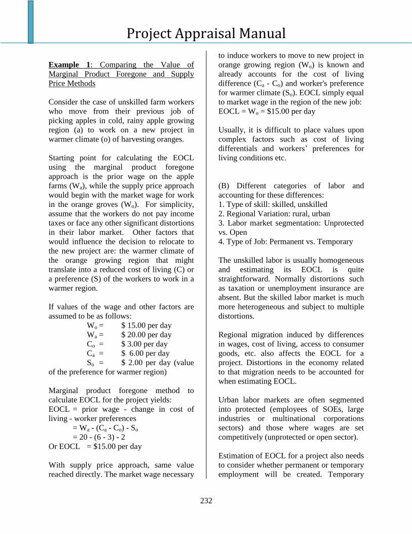
Project Appraisal Manual
232
Example 1: Comparing the Value of
Marginal Product Foregone and Supply
Price Methods
Consider the case of unskilled farm workers
who move from their previous job of
picking apples in cold, rainy apple growing
region (a) to work on a new project in
warmer climate (o) of harvesting oranges.
Starting point for calculating the EOCL
using the marginal product foregone
approach is the prior wage on the apple
farms (Wa), while the supply price approach
would begin with the market wage for work
in the orange groves (Wo). For simplicity,
assume that the workers do not pay income
taxes or face any other significant distortions
in their labor market. Other factors that
would influence the decision to relocate to
the new project are: the warmer climate of
the orange growing region that might
translate into a reduced cost of living (C) or
a preference (S) of the workers to work in a
warmer region.
If values of the wage and other factors are
assumed to be as follows:
Wo = $ 15.00 per day
Wa = $ 20.00 per day
Co = $ 3.00 per day
Ca = $ 6.00 per day
So = $ 2.00 per day (value
of the preference for warmer region)
Marginal product foregone method to
calculate EOCL for the project yields:
EOCL = prior wage - change in cost of
living - worker preferences
= Wa - (Ca - Co) - So
= 20 - (6 - 3) - 2
Or EOCL = $15.00 per day
With supply price approach, same value
reached directly. The market wage necessary
to induce workers to move to new project in
orange growing region (Wo) is known and
already accounts for the cost of living
difference (Ca - Co) and worker's preference
for warmer climate (So). EOCL simply equal
to market wage in the region of the new job:
EOCL = Wo = $15.00 per day
Usually, it is difficult to place values upon
complex factors such as cost of living
differentials and workers’ preferences for
living conditions etc.
(B) Different categories of labor and
accounting for these differences:
1. Type of skill: skilled, unskilled
2. Regional Variation: rural, urban
3. Labor market segmentation: Unprotected
vs. Open
4. Type of Job: Permanent vs. Temporary
The unskilled labor is usually homogeneous
and estimating its EOCL is quite
straightforward. Normally distortions such
as taxation or unemployment insurance are
absent. But the skilled labor market is much
more heterogeneous and subject to multiple
distortions.
Regional migration induced by differences
in wages, cost of living, access to consumer
goods, etc. also affects the EOCL for a
project. Distortions in the economy related
to that migration needs to be accounted for
when estimating EOCL.
Urban labor markets are often segmented
into protected (employees of SOEs, large
industries or multinational corporations
sectors) and those where wages are set
competitively (unprotected or open sector).
Estimation of EOCL for a project also needs
to consider whether permanent or temporary
employment will be created. Temporary
Project Appraisal Manual
233
positions (tourism, construction) lead to
greater turnover and create conditions for
voluntary unemployment and thus causing
additional costs to the economy.
II. The Economic Opportunity Cost of
Unskilled Rural Labor
Supply Price Approach - Three steps are
involved:
(i) Determine the minimum gross-of-tax
wage (W) needed to attract sufficient
unskilled labor;
(ii) Identify distortions in the labor market
such as income taxes or unemployment
insurance benefits;
(iii) Determine EOCL by adjusting for
distortions.
Several cases may arise in this group.
Case I : No seasonal variations in the
market wage and no distortions in the
unskilled labor market. It follows that
supply price of labor equals the prevailing
market wage (Wu). No need to make further
adjustments because there are no distortions.
(1) EOCLu = W
u = Supply Price of
Unskilled Labor
Case II: Estimation of EOCL of unskilled
labor for a project where demand of workers
is same throughout the year while the
market wage varies due to external factors
affecting labor market. If no tax distortions,
the EOCL is the average of the monthly or
weekly market wage rates (Wu
i) for the
duration of the project.
n n
(2) EOCLU = LiW
ui /
Li i=1 i=1
where:
n = the number of periods over which the
EOCL is being estimated
i = the period of time
Li= the number of people employed during
period i.
Seasonal variations: It is quite common to
have seasonal variation in the size of the
employed work force in rural areas. In this
case, EOCL is a weighted average of the
different unskilled wage rates throughout the
year.
This equals the sum of unskilled wage rate
for each particular season or wage period
(Wu
i) times the proportion (Ki) of the total
amount of unskilled labor employed by the
project in that period. n
As Ki = Li / Li (Eq. 2) can be rewritten as: i=1
n
(3) EOCLu = (Ki W
ui)
i=1
where: n = the total number of periods; i =
the period of time.
Example 2: Sugar Factory hires
Unskilled Labor in a Rural Area
A labor-intensive sugar project requires
unskilled workers on a temporary basis and
pays a wage of 180 dollars per month (Wu
p).
The working conditions are identical to
those prevailing in the labor market. Table 1
(column 3) shows the project's monthly
requirements for person-months and in
column (2) the monthly market wage rates
(Wu
i) that agricultural labor would be
willing to work for this project.
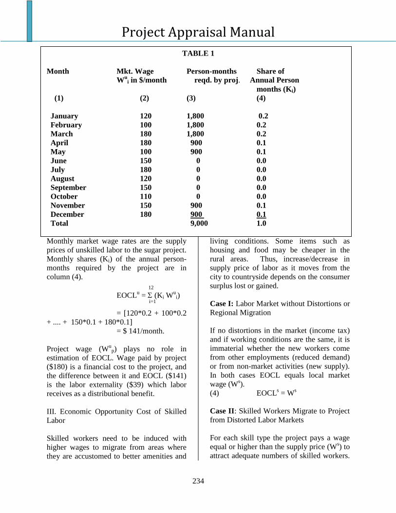
Project Appraisal Manual
234
TABLE 1
Month Mkt. Wage Person-months Share of
Wu
i in $/month reqd. by proj. Annual Person
months (Ki)
(1) (2) (3) (4)
January 120 1,800 0.2
February 100 1,800 0.2
March 180 1,800 0.2
April 180 900 0.1
May 100 900 0.1
June 150 0 0.0
July 180 0 0.0
August 120 0 0.0
September 150 0 0.0
October 110 0 0.0
November 150 900 0.1
December 180 900 0.1
Total 9,000 1.0
Monthly market wage rates are the supply
prices of unskilled labor to the sugar project.
Monthly shares (Ki) of the annual person-
months required by the project are in
column (4).
12
EOCLu = (Ki W
ui)
i=1
= [120*0.2 + 100*0.2
+ .... + 150*0.1 + 180*0.1]
= $ 141/month.
Project wage (Wu
p) plays no role in
estimation of EOCL. Wage paid by project
($180) is a financial cost to the project, and
the difference between it and EOCL ($141)
is the labor externality ($39) which labor
receives as a distributional benefit.
III. Economic Opportunity Cost of Skilled
Labor
Skilled workers need to be induced with
higher wages to migrate from areas where
they are accustomed to better amenities and
living conditions. Some items such as
housing and food may be cheaper in the
rural areas. Thus, increase/decrease in
supply price of labor as it moves from the
city to countryside depends on the consumer
surplus lost or gained.
Case I: Labor Market without Distortions or
Regional Migration
If no distortions in the market (income tax)
and if working conditions are the same, it is
immaterial whether the new workers come
from other employments (reduced demand)
or from non-market activities (new supply).
In both cases EOCL equals local market
wage (Ws).
(4) EOCLs = W
s
Case II: Skilled Workers Migrate to Project
from Distorted Labor Markets
For each skill type the project pays a wage
equal or higher than the supply price (Ws) to
attract adequate numbers of skilled workers.
Project Appraisal Manual
235
EOCL for each type of labor equals the
gross-of-tax supply price to the project of
that type, less any taxes now paid by these
workers on the project, plus any taxes lost
due to movement of labor to project.
Migration of workers from other regions to
the project causes labor supply (S) in the
sending region to decrease, thus shifting the
labor supply curve leftward to the new
position S'.
At the original net-of-tax wage for skilled
labor (Wsa(1 - t)) in the sending region, the
migration to the project causes a decrease in
the available supply from Q0 to Q1. For
equilibrium in labor market, wage must
increase to Ws'a(1 - t). This higher wage
reduces demand in the sending regions.
Higher wage rates induce some skilled
workers to enter the formal labor (or
overtime) market increasing the quantity of
skilled labor supplied from Q1 to Q2.
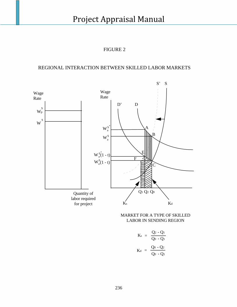
Project Appraisal Manual
236
S’ S
D’ D
Q1 Q2 Q0
KdKs
Wage
Rate
W S’a
Wa
S
W S’a (1 - t)
Wa
S(1 - t)
A
B
E
C
F
Ks =Q2 - Q1
Q0 - Q1
Kd =Q0 - Q2
Q0 - Q1
MARKET FOR A TYPE OF SKILLED
LABOR IN SENDING REGION
Wage
Rate
WS
Quantity of
labor required
for project
Wp
S
FIGURE 2
REGIONAL INTERACTION BETWEEN SKILLED LABOR MARKETS
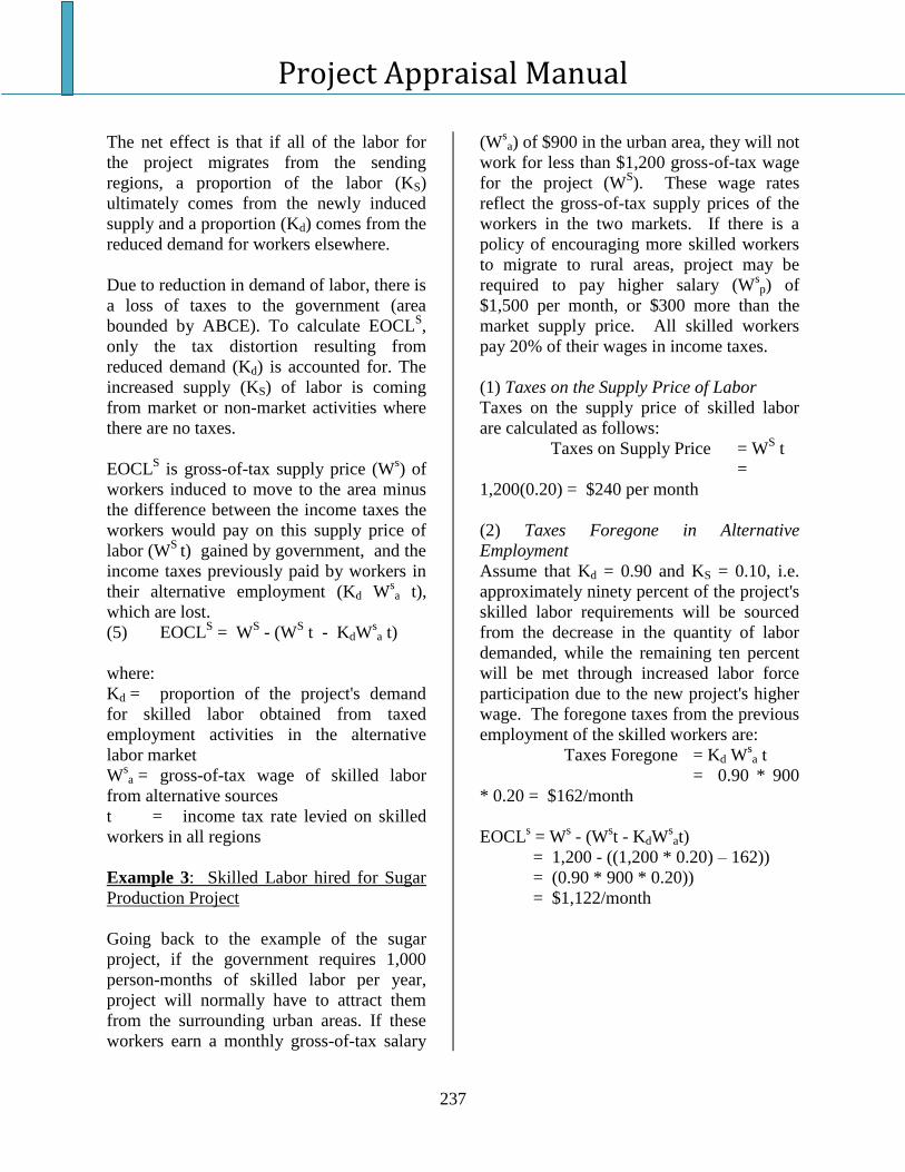
Project Appraisal Manual
237
The net effect is that if all of the labor for
the project migrates from the sending
regions, a proportion of the labor (KS)
ultimately comes from the newly induced
supply and a proportion (Kd) comes from the
reduced demand for workers elsewhere.
Due to reduction in demand of labor, there is
a loss of taxes to the government (area
bounded by ABCE). To calculate EOCLS,
only the tax distortion resulting from
reduced demand (Kd) is accounted for. The
increased supply (KS) of labor is coming
from market or non-market activities where
there are no taxes.
EOCLS is gross-of-tax supply price (W
s) of
workers induced to move to the area minus
the difference between the income taxes the
workers would pay on this supply price of
labor (WS
t) gained by government, and the
income taxes previously paid by workers in
their alternative employment (Kd Wsa t),
which are lost.
(5) EOCLS = W
S - (W
S t - KdW
sa t)
where:
Kd = proportion of the project's demand
for skilled labor obtained from taxed
employment activities in the alternative
labor market
Wsa = gross-of-tax wage of skilled labor
from alternative sources
t = income tax rate levied on skilled
workers in all regions
Example 3: Skilled Labor hired for Sugar
Production Project
Going back to the example of the sugar
project, if the government requires 1,000
person-months of skilled labor per year,
project will normally have to attract them
from the surrounding urban areas. If these
workers earn a monthly gross-of-tax salary
(Wsa) of $900 in the urban area, they will not
work for less than $1,200 gross-of-tax wage
for the project (WS). These wage rates
reflect the gross-of-tax supply prices of the
workers in the two markets. If there is a
policy of encouraging more skilled workers
to migrate to rural areas, project may be
required to pay higher salary (Wsp) of
$1,500 per month, or $300 more than the
market supply price. All skilled workers
pay 20% of their wages in income taxes.
(1) Taxes on the Supply Price of Labor
Taxes on the supply price of skilled labor
are calculated as follows:
Taxes on Supply Price = WS t
=
1,200(0.20) = $240 per month
(2) Taxes Foregone in Alternative
Employment
Assume that Kd = 0.90 and KS = 0.10, i.e.
approximately ninety percent of the project's
skilled labor requirements will be sourced
from the decrease in the quantity of labor
demanded, while the remaining ten percent
will be met through increased labor force
participation due to the new project's higher
wage. The foregone taxes from the previous
employment of the skilled workers are:
Taxes Foregone = Kd Wsa t
= 0.90 * 900
* 0.20 = $162/month
EOCLs = W
s - (W
st - KdW
sat)
= 1,200 - ((1,200 * 0.20) – 162))
= (0.90 * 900 * 0.20))
= $1,122/month
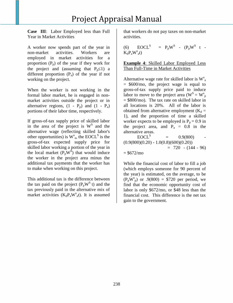
Project Appraisal Manual
238
Case III: Labor Employed less than Full
Year in Market Activities
A worker now spends part of the year in
non-market activities. Workers are
employed in market activities for a
proportion (Pp) of the year if they work for
the project and (assuming that Pp1) a
different proportion (Pa) of the year if not
working on the project.
When the worker is not working in the
formal labor market, he is engaged in non-
market activities outside the project or in
alternative regions, (1 - Pp) and (1 - Pa)
portions of their labor time, respectively.
If gross-of-tax supply price of skilled labor
in the area of the project is WS and the
alternative wage (reflecting skilled labor's
other opportunities) is Wsa, the EOCL
S is the
gross-of-tax expected supply price for
skilled labor working a portion of the year in
the local market (PpWS) that would induce
the worker in the project area minus the
additional tax payments that the worker has
to make when working on this project.
This additional tax is the difference between
the tax paid on the project (PpWS
t) and the
tax previously paid in the alternative mix of
market activities (KdPaWsat). It is assumed
that workers do not pay taxes on non-market
activities.
(6) EOCLS = PpW
S - (PpW
S t -
KdPaWsat)
Example 4: Skilled Labor Employed Less
Than Full-Time in Market Activities
Alternative wage rate for skilled labor is Wsa
= $600/mo, the project wage is equal to
gross-of-tax supply price paid to induce
labor to move to the project area (WS
= Wsp
= $800/mo). The tax rate on skilled labor in
all locations is 20%. All of the labor is
obtained from alternative employment (Kd =
1), and the proportion of time a skilled
worker expects to be employed is Pp = 0.9 in
the project area, and Pa = 0.8 in the
alternative areas.
EOCLS
= 0.9(800) -
(0.9(800)(0.20) - 1.0(0.8)(600)(0.20))
= 720 - (144 - 96)
= $672/mo
While the financial cost of labor to fill a job
(which employs someone for 90 percent of
the year) is estimated, on the average, to be
(PpWsp) or .9(800) = $720 per period, we
find that the economic opportunity cost of
labor is only $672/mo, or $48 less than the
financial cost. This difference is the net tax
gain to the government.