modeling of belt-drives using a large deformation finite element formulation
TRANSCRIPT
Nonlinear Dynamics (2006) 43: 239–256
DOI: 10.1007/s11071-006-7749-5 c© Springer 2006
Modeling of Belt-Drives Using a Large Deformation FiniteElement Formulation
KIMMO S. KERKKANEN1,∗, DANIEL GARCIA-VALLEJO2, and AKI M. MIKKOLA1
1Institute of Mechatronics and Virtual Engineering, Department of Mechanical Engineering, Lappeenranta Universityof Technology, P.O. Box 20, FIN-53851 Lappeenranta, Finland; 2Department of Mechanical and Materials Engineering,University of Seville, Camino de los Descubrimientos s/n, 41092 Seville, Spain;∗Author for correspondence (e-mail: [email protected]; fax: +358-5-621-2499)
(Received: 27 October 2004; accepted: 13 May 2005)
Abstract. In this paper, the applicability of the absolute nodal coordinate formulation for the modeling of belt-drive systems
is studied. A successful and effective analyzing method for belt-drive systems requires the exact modeling of the rigid body
inertia during an arbitrary rigid body motion, accounting of shear deformation, description of highly nonlinear deformations, and
a simple as well as realistic description of the contact. The absolute nodal coordinate formulation meets the challenge and is a
promising approach for the modeling of belt-drive systems. In this study, a recently proposed two-dimensional shear deformable
beam element based on the absolute nodal coordinate formulation has been modified to obtain a belt-like element. In the original
element, a continuum mechanics approach is applied to the exact displacement field of the shear deformable beam. The belt-like
element allows the user to control the axial and bending stiffness through the use of two parameters. In this study, the interaction
between the belt and the pulleys is modeled using an elastic approach in which the contact is accounted for by the inclusion of
a set of external forces that depend on the penetration between the belt and pulley. When using the absolute nodal coordinate
formulation, the contact forces can be distributed over the length of the element due to the use of high-order polynomials. This is
different from other approaches that are used in the modeling of belt-drives. Static and dynamic analysis are used in this study to
show the performance of the distributed contact force model and the proposed belt-like element, which is able to model highly
nonlinear deformations. Applying these two contributions to the modeling of belt-drive systems, instead of contact forces applied
at nodes and low-order elements, leads to a considerable reduction in the degrees of freedom.
Key words: beam element, belt-drive, large deformation, multibody application
1. Introduction
A typical use for the belt-drives is power transmission between rotational machine elements. Accord-
ingly, belt-drives are widely used in various ranges of applications including domestic appliances as
well as automotive technology. These mechanical systems involve pulleys and belts, which dynamically
contact each other through a dry friction interface. The tension of the belt transitions ranges from small
to a large tension and vice versa during the operation. The life of the belt-drive depends critically on
the tension magnitudes in the belt spans. Another significant factor in the life of the belt-drive is the
sliding wear of the belt caused by creeping against the pulley. In the long run, this wear may deteriorate
the surface of the belt leading to changes in the friction characteristics of the belt. As a result, noisy
operation and other problems may take place. It is also interesting to notice the analogy between the
belt-drives and calendering. There are many critical and challenging applications in paper and metal
industry, where the passage of an elastic strip or sheet of material through the nip between different kinds
of rollers is included. The theory and methods used in modeling the belt-drives could be potentially
utilizable and worth extending to the modeling of calendering in the paper-making process. For these
reasons, a detailed and computationally efficient model of the belt-drive, which is capable of accurately
240 K. S. Kerkkanen et al.
predicting the belt dynamics and the contribution of the contact forces between the belt and pulley, is
beneficial in the product-development process.
A compact review of the research of the belt-drives is given by Leamy and Wasfy in Ref. [1], where
it is also shown that the research of the belt-drives can be divided into belt-drive mechanics studies
and serpentine belt-drive dynamic response studies. According to the authors of Ref. [1], the belt-drive
mechanics studies have not often considered the dynamic excitation, while the frictional belt-pulley
modeling in the serpentine belt-drive studies has been typically idealized. As a result, the connection
between belt-drive mechanics and the dynamic response of serpentine belt-drives has been weak due
to the nature of the modeling methods. The problem has been studied by Leamy et al. in Refs. [2–4],
where the simplified dynamic models for small and large rotational speeds are introduced. In Ref. [1]
Leamy et al. have proposed a general dynamic finite element model of belt-drive systems. In the study,
the belt is modeled using truss elements including detailed frictional contact [1, 5]. The finite elements
use only Cartesian coordinates of the nodes as degrees of freedom, and all degrees of freedom are
defined directly in a global inertial reference frame. The contact forces are applied at the nodes only.
This leads to a large number of degrees of freedom, when the accurate representation of the circular
boundaries of the pulleys is considered. The equations of motion are formulated using a total Lagrangian
formulation. The effect of bending stiffness on the dynamic and steady-state responses of belt-drives
can be accounted for using three node beam elements based on the torsional-spring formulation [6, 7].
The authors of Refs. [1, 5, 7] demonstrate that the results of the proposed models and analytical values
are in good agreement for discretizations with 38 (three node beam elements, 154 degrees of freedom)
or 100 (truss elements, 202 degrees of freedom) elements per half pulley.
There are four main requirements that should be satisfied when modeling belt-drive systems. First,
exact modeling of the rigid body inertia resulting in zero strains must be obtained. This is due to the
fact that a piece of the belt, i.e. an element undergoes large relative translation and rotations. Second,
the effect of the shear deformation must be considered as pointed out in Ref. [8]. The third requirement
is related to the description of highly nonlinear deformations that have to be described in order to
obtain a reasonable number of degrees of freedom in the model. The last essential requirement for the
formulation used to model belt-drive systems is a simple and effective description of the contact between
the belt and the pulleys. The objective of this study is to find out the applicability of the absolute nodal
coordinate formulation for modeling belt-drive systems. The absolute coordinate formulation leads to an
exact description of an arbitrary rigid body motion, a constant mass matrix and a capability of modeling
nonlinear deformations [9–11].
It is important to note that in flexible multi-body dynamics, the deformation of the elastic bodies
is often defined with respect to a body reference using mode shapes. These modes are described in
body-fixed or floating coordinate systems. When the contact of the bodies of the system is activated,
one may have to change the coordinate system or redefine the new set of mode shapes to achieve
a correct description of the deformation of the elastic bodies. In addition, nonlinear deformation is
difficult to determine using the mode shapes. These problems can be avoided using the absolute nodal
coordinate formulation, where the deformations of the bodies are described in the global coordinate
system.
In most of the applications, the belts are usually made from composite materials. Therefore, the
belts exhibit a non-isotropic behavior that cannot be captured using a conventional beam element. For
this reason, it is desirable to formulate an element that allows for reducing the bending stiffness of
the element. In this study, a new belt-like element is introduced by modifying the recently proposed
two-dimensional shear deformable beam element, where a continuum mechanics approach is applied
to the exact displacement field of the shear deformable beam [12].
Modeling of Belt-Drives 241
This paper is organized as follows. A description of the two-dimensional beam element used which is
based on the absolute nodal coordinate formulation including the nodal coordinates, shape functions, the
elastic forces, and the exact description of the kinematics of the beam is given in Section 2. In Sections
3 and 4, the modeling of the frictional contact between the pulleys and the belt, the modeling of the joint
constraint and the equation of motion are presented in detail. The description of the belt-drive system
studied and the numerical results of several examples are demonstrated in Section 5. In the last section,
a summary and the conclusions drawn from the results of this study are presented.
2. Formulation of the Finite Element Used
The beam finite element used in this study is based on a two-dimensional element originally proposed by
Dufva et al. [12]. This shear deformable element is based on the absolute nodal coordinate formulation
and it includes an accurate expression of the elastic forces. In the element, a continuum mechanics
approach is utilized in the exact displacement field of the shear deformable beam. This leads to the
capability of accurately predicting the nonlinear deformations without suffering from shear or Poisson’s
locking [12].
The behavior of the belts strongly depends on the kinds of loads they are subjected to. In most of the
cases, the stiffness of the belt in bending is usually much lower than in axial deformations due to the use
of the composite material. For this reason, the beam element proposed by Dufva et al. [12] is slightly
modified to obtain an element with reduced bending stiffness. In the following, kinematics and strain
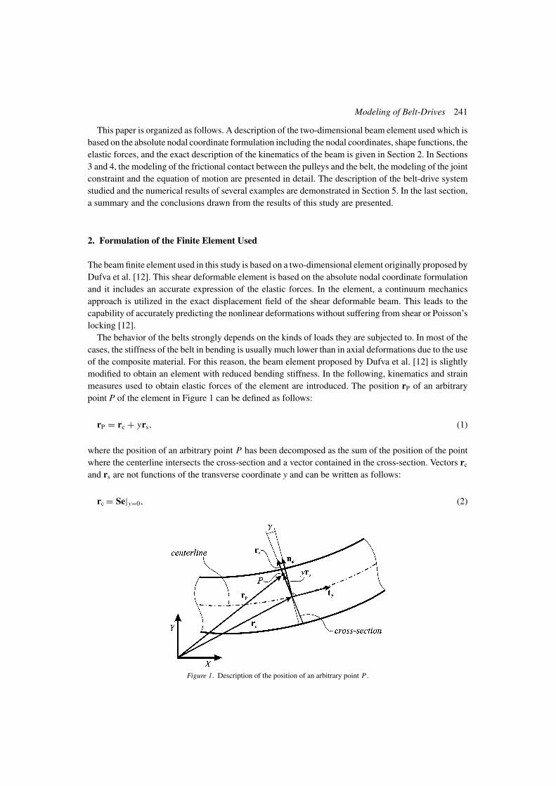
measures used to obtain elastic forces of the element are introduced. The position rP of an arbitrary
point P of the element in Figure 1 can be defined as follows:
rP = rc + yrs, (1)
where the position of an arbitrary point P has been decomposed as the sum of the position of the point
where the centerline intersects the cross-section and a vector contained in the cross-section. Vectors rc
and rs are not functions of the transverse coordinate y and can be written as follows:
rc = Se|y=0, (2)
Figure 1. Description of the position of an arbitrary point P .
242 K. S. Kerkkanen et al.
rs = (I + I sin γ )Itψ, (3)
where I is an identity matrix, γ is a shear angle as shown in Figure 1 and tψ is a vector that defines
the tangent of the beam’s centerline. In Equation (3), vector rs is obtained by two successive rotations
over vector tψ . First, vector tψ is rotated 90◦ using matrix I leading to a vector nψ shown in Figure 1,
and after that an angle of γ due to shear deformation. In Equation (3), skew symmetric matrix I is as
follows:
I =[
0 −1
1 0
]. (4)
Vector tψ can be expressed using the global position of the centerline as follows:
tψ =∂rc
∂x∥∥ ∂rc
∂x
∥∥ . (5)
In Equation (2) S is the element shape function matrix, which in the case of a shear deformable planar
beam element contains cubic terms in x and linear terms in y. In Equation (2) e is the nodal coordinate
vector, which consists of the global position vector and the slope vectors that define the global orientation
of the centerline and the orientation of the height coordinates of the cross-section of the beam. The
vector e can be written for node i of the element as follows:
ei =[
riT ∂riT
∂x
∂riT
∂y
]T
, (6)
where ri is the global position vector of node i and vectors ∂riT/∂x and ∂riT/∂y are the position vector
gradients, i.e. the slopes of node i.The linear distribution of the shear angle can be obtained using a method that resembles the mixed
interpolation technique as follows:
sin γ = (sin γ )i
(1 − x
L
)+ (sin γ ) j x
L. (7)
In Equation (7), (sin γ )i and (sin γ ) j are the components of the shear strains at the nodal points i and jof the element, respectively, x is the element longitudinal coordinate and L is the length of the element
[12].
The strain energy can be expressed as the sum of the strain energy associated with each one of the
components of the strain tensor as follows:
U = 1
2
∫V
(Eε2
xx + Eε2yy + 4ksGε2
xy
)dV . (8)
In Equation (8) E is Young’s modulus, ks the shear correction factor, G the shear modulus and V the
volume of the element. Note that initially the beam is assumed to be coincident with the global coordinate
system and not curved. The strain components εxx and εxy can be calculated using Green–Lagrange
measures as follows:
εxx = 1
2
[∂rT
∂x
∂r∂x
− 1
], (9)
Modeling of Belt-Drives 243
εxy = 1
2
[∂rT
∂x
∂r∂y
]. (10)
The strain component εyy in the beam transverse direction can be defined employing the position vector
gradient ∂r/∂y at the nodal points together with linear interpolation functions, as explained in Ref. [12].
After algebraic manipulations, the terms involved in Equation (8) can be rewritten as follows:
ε2xx = 1
4
(rT
c,x rc,x − 1)2 + (
rTc,x rc,x − 1
)(rT
c,x rs,x − 1)y +
+ [(rT
c,x rs,x)2 + 1
2
(rT
c,x rc,x − 1)(
rTs,x rs,x
)]y2 +
(11)
+ (rT
c,x rs,x)(
rTs,x rs,x
)y3 + 1
4
(rT
s,x rs,x)2
y4,
ε2xy = 1
4
(rT
c,x rs
)2 + 1
2
(rT
c,x rs
)(rT
s,x rs
)y + 1
4
(rT
s,x rs
)2y2. (12)
Loads that cause bending as well as those that cause elongation of the element induce strains in the
longitudinal direction. For this reason, the strain energies due to axial and bending solicitations are both
contained in the first term of Equation (8). It is important to note that the strain due to axial loads is
supposed to be constant along the thickness of the element, and consequently, the strain energy per unit
of volume due to elongation of the element must be independent of the coordinate y. Moreover, the
elongation εl of the centerline of the element can be written as follows [13]:
εl = 1
2
(rT
c,x rc,x − 1). (13)
According to Equation (13), the part of ε2xx corresponding to the strain energy associated with an
elongation of the element can be easily identified in Equation (11). Therefore, in order to modify the
bending stiffness of the element, coefficients α1 and α2 are included determining the importance of each
term in the equation of the strain energy. Due to the symmetry of the cross-section of the element, terms
that are multiplied by y and y3 in Equations (11) and (12) vanish after integration over the y coordinate.
Thus, using Equations (11) and (12), the first and last terms in the right hand side of Equation (8) can
be written as follows:
1
2
∫V
Eε2xx dV = E
2
∫V
[α1
4
(rT
c,x rc,x − 1)2 + α2
[(rT
c,x rs,x)2 + 1
2
(rT
c,x rc,x − 1)(
rTs,x rs,x
)]y2
+ α2
4
(rT
s,x rs,x)2
y4
]dV, (14)
1
2
∫V
4ksGε2xy dV = 2ksG
∫V
[α2
4
(rT
c,x rs
)2 + α2
4
(rT
s,x rs
)2y2
]dV . (15)
Note that since there should be no tangential deformation εxy in a pure axial strength state, the part of
the energy due to transverse strain is affected by coefficient α2. As can be seen from Equations (14)
and (15), parameters α1 and α2 can be used to modify the Young’s modulus used to calculate the elastic
forces due to axial elongation and the Young’s modulus used in bending deformation. In case of small
strains, parameters α1 and α2 linearly affect the axial and bending stiffness of the element. The vector

244 K. S. Kerkkanen et al.
of the elastic forces can be defined using the strain energy U as follows:
Qe = −(
∂U
∂e
)T
. (16)
3. Modeling of the Frictional Contact
In power transmission systems that use belts and pulleys, the belt is constrained to move over the
surface of the pulley. The contact between both solids must include frictional forces, which are, in fact,
responsible for the transmission of motion from the pulley to the belt and vice versa. In this study,
frictional contact between the pulleys and the belt is modeled applying a method that is based on the
studies of Leamy and Wasfy [1, 7]. In this method, a penalty formulation is applied with a Coulomb-like
tri-linear creep-rate dependent friction. The advantages of the law are numerical stability and physical
relevance in the case of small sliding velocity [5].
In the models proposed by Leamy and Wasfy [1, 7], the forces are applied to the nodes of the low-
order elements. A normal reaction force and a tangential friction force are generated when a node on
the finite element is in contact with the surface of the constraint. The contact forces depend significantly
on the closest distance between the node and the contact surface. The contact exists when the node is
inside the contact body. The results of their models, where low-order elements are used, are based on
the discretizations from 38 (154 degrees of freedom) up to 100 (202 degrees of freedom) elements per
half pulley. It is important to reiterate that one of the main objectives in this study is to use the absolute
nodal coordinate formulation in order to decrease the number of the needed elements and degrees of
freedom.
In contrast to the study of Leamy and Wasfy, the two-dimensional high-order elements used in this
study are capable of reproducing curved shapes using a small number of elements. It is shown in Ref.
[12] that the use of only four elements enables the bending of a cantilever beam into a circle when a
certain concentrated moment is applied at the free end. Since the element can be curved over the surface
of the pulley, in contrast to the linear low-order element used in the models proposed by Leamy and
Wasfy [1, 7], the contact forces do not need to be applied at the nodes only. The use of a high-order
element enables the distribution of the contact forces along the length of the element. Although the
main idea of the model of the contact forces remains the same as in the models of Leamy and Wasfy,
the procedure used in this study is subtly different, as it is shown in detail in this section.
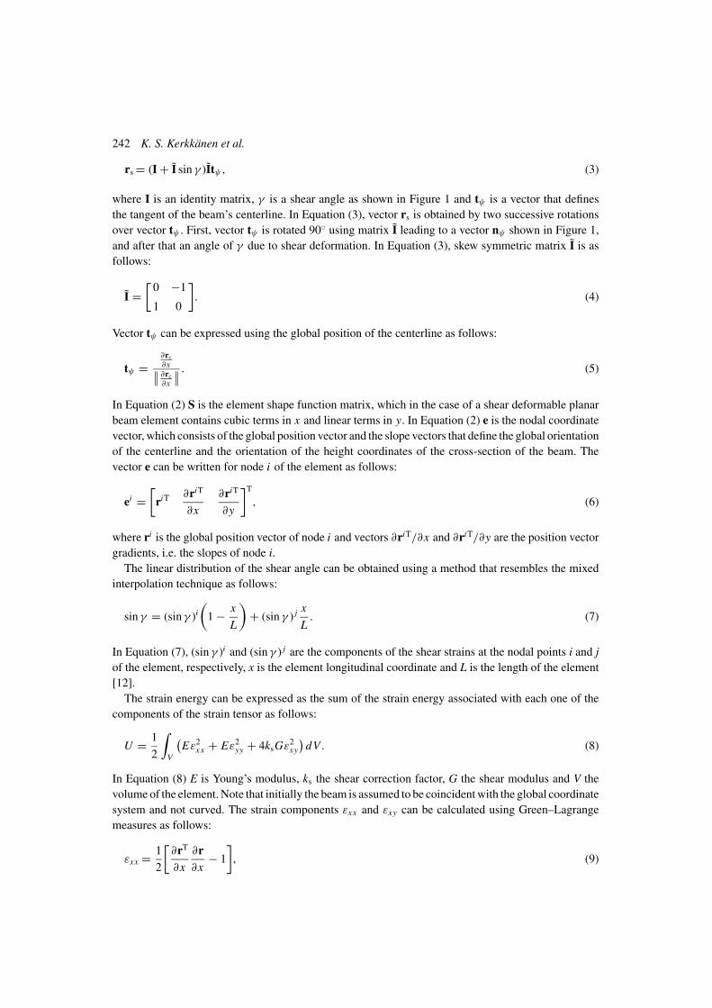
In the contact description, the element is allowed to penetrate the pulley at a certain distance d as
depicted in Figure 2, and, as a result of this penetration, a force, which is perpendicular to the surface of
the pulley and directed along vector n appears. This force is proportional to the penetration d and to its
time-derivative d . Due to the capability of the high-order element of adopting a curved configuration,
the penetration is a function of the longitudinal coordinate of the element, x, and as a consequence, the
normal and tangential contact forces also depend on x. Thus, the distributed normal reaction force fn,
between the pulley and the belt can be written as follows:
fn ={
(kpd + cpd)n, d ≥ 0
0, d < 0. (17)
In Equation (17), n is the unit normal vector at the contact surface, d denotes the closest distance between
an arbitrary point in the element and the contact surface and kp and cp are the stiffness and damping
coefficient per unit length of the penalty force, respectively.
Modeling of Belt-Drives 245
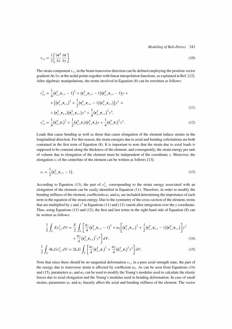
Figure 2. Description of the distributed contact forces.
Contact searching is executed through evaluation of the penetration distance d of an arbitrary point
in the centerline of the element, which can be defined using the following equations:
d = R −√
(r − rO )T(r − rO ). (18)
In Equation (18) R is the radius of the circular constraint, and r the location of an arbitrary point in
the centerline of the element, which can be evaluated using the shape function and the vector of the
nodal coordinates of the element. In Equation (18) ro is the location of the center of the constraint in
the global coordinate system. Superscripts that refer to the number of elements have been eliminated
for simplicity.
The normal unit vector n to the surface of the circular constraint can be expressed as follows:
n = r − rO√(r − rO )T(r − rO )
. (19)
In the Coulomb model, tangential forces due to friction are point-wise proportional to the modulus
of the normal forces. However, considering the pure Coulomb model, the integration of the equation
of motion results in a cumbersome process. The use of a tri-linear creep-rate law that depends on the
relative velocity between the contacting surfaces alleviates the friction model difficulties; therefore, the
resulting system of equations is, in a computational sense, less expensive to integrate.
The tangential friction force is governed by the creep-rate dependent frictional law and can be
expressed as follows:
ft = −μ(vt )‖fn‖t. (20)
In Equation (20) ft is the distributed tangential friction force, μ(vt) is the friction coefficient that
depends on the relative tangent velocity vt, and ‖ ·‖ denotes the L2 norm. In addition, t is the unit vector
perpendicular to the normal n as shown in Figure 2, and can be calculated as
t = In, (21)
where I can be written as introduced in Equation (4). The tangent relative velocity between the surfaces
in contact can be calculated in a straightforward manner since the pulleys are assumed to rotate around
246 K. S. Kerkkanen et al.
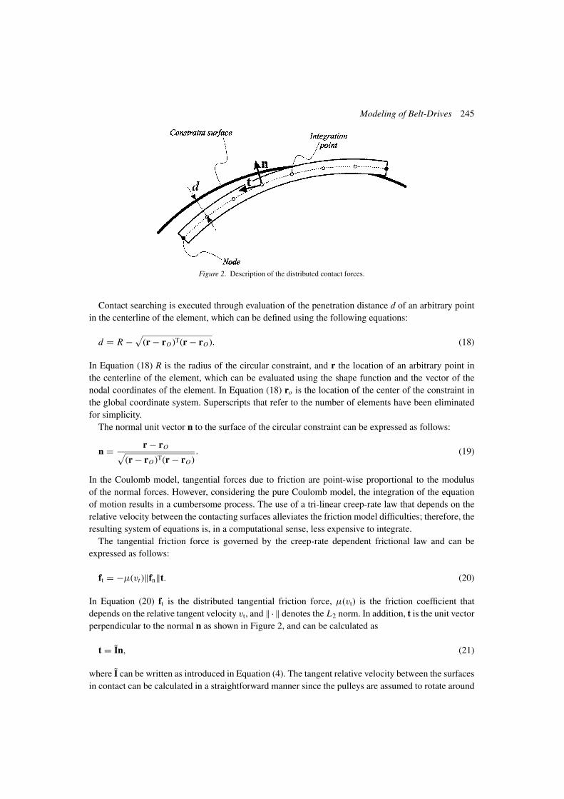
Figure 3. Tri-linear creep-rate dependent law [5].
their center of masses. Assuming that the angular velocity of the pulley is ω, the relative tangent velocity
of an arbitrary point in the centerline of the element can be written as follows:
vt = tT(r − ωRt). (22)
The dependency of the friction coefficient on the tangent velocity is shown in Figure 3.
The parameter νs in Figure 3 is the slope of the friction force with respect to tangent velocity at small
sliding velocities. The angular velocity ω of the pulley is usually an explicit function of time for a driver
pulley. In contrast, for a driven pulley, the moment equilibrium equation can be included in the system
of equations of motion considering the angle rotated by the pulley as a generalized coordinate. This
equation can be written as follows:
I θ =Ne∑
i=1
∫ Li
0
((R − d)n × (−ft))i dx + Ta. (23)
In Equation (23) I is the mass moment of inertia of the driven pulley, θ the angular acceleration, index
i refers to the number of elements, Ne is the number of elements of the model, Li the length of the
element i and Ta the possible opposing torque applied by the driven accessories on the constraint.
It is important to note that the model does not place any restriction for the possible slippage of a
point in the centerline. The use of the slopes as nodal coordinates enables the element to adopt curved
configurations. Due to this feature the normal and friction forces can be different from point to point
and, indeed, it should be possible to find areas of slippage and areas of sticking within the same element.
The virtual work done by the frictional contact forces can be used to obtain the expression of the
generalized frictional contact forces. Thus, the virtual work of the friction forces can be written as
δW =∫ L
0
δrT(fn + ft) dx = δeT
∫ L
0
ST0 (fn + ft) dx = δeTQc, (24)
where L is the length of the element and S0 is the shape function of the element evaluated at the centerline
of the beam element, that is, y = 0. The integral in Equation (24) is complicated to evaluate symbolically
and, for this reason, a Gaussian quadrature integration formula is employed to solve the integral of the
virtual work. Since the normal and friction forces are not smooth functions, a high enough number of
Modeling of Belt-Drives 247
integration points must be used. In addition, the number of integration points is related to the accuracy
of the definition of the slippage area of the element, as long as the information of sliding is obtained at
the integration points.
In the finite element assembling procedure, the distributed contact forces are converted to the gen-
eralized friction contact forces (i.e. equivalent nodal force) as expressed in Equation (24). This is
accomplished using the shape function matrix, which is a crucial step if the belt is modeled using a low
number of elements. Naturally, in the finite element sense, the use of the distributed contact force could
be replaced by a large number of discrete forces [1, 5, 7]. The use of the distributed contact forces with
the high-order elements allows reducing the number of elements and, therefore, the number of degrees
of freedom, since the curving of the elements into the circular shape of the pulley is no longer vis major.
It is worth remarking the importance of using a small number of elements to model the contact between
the pulley and the belt. The reason being that in belt and pulley applications, the distance between the
centers of the pulleys, the span length, is usually much larger than the arc length of the pulleys. It is
also usual that the pulleys are very different in size because of changes in velocities and torques. In this
case, the smallest pulley forces to use an excessive number of elements for the larger one. Hence, the
total number of elements in the model can be considerably decreased with a reduction in the number of
elements needed per pulley. Since, when using the Lagrangian mesh, all the elements of the belt have to
come in contact with the pulleys sooner or later, there is no possibility to use different element lengths.
When using the absolute nodal coordinate formulation, it is also easy to detect the possibility of the
element contact before the contact calculation procedure. Then, if the element cannot be in contact with
a pulley due to its location in the middle of one of the spans, there is no reason to check the forces in the
integration points. Neither is there need to find the limits of the contact area a priori since eventually
the integration point is checked when evaluating the integral in Equation (24). Based on these features,
the proposed model leads to the inclusion of contact in a systematic manner.
4. Modeling of the Joint Constraint and Equations of Motion
As in many other multibody applications, Lagrange equations can be used to obtain the equations of
motion of the belt-drive system. The belt is essentially treated as a beam whose ends are joined together
forming a closed-loop structure. Due to the use of absolute nodal coordinates, the constraints that come
from the rigid joint are linear. These linear constraints can be added to the equations of motion by the
use of Lagrange multipliers. On the other hand, the contact between the belt and the pulleys is simulated
by the inclusion of a set of external forces as explained in the previous section. Differentiating the
constraint equations twice with respect to time, the system equations of motion can be written as
[M CT
e
Ce 0
][eλ
]=
[QQd
], (25)
where M is the constant mass matrix of the system [11], Ce the Jacobian of the constraint equations, ethe acceleration vector of the nodal coordinates, λ the vector of Lagrange multipliers, Q the generalized
force vector that includes contact and elastic forces and Qd is obtained through differentiation of the
constraints as Cee = Qd.
It is worth remarking the convenience of using the absolute nodal coordinate formulation when
dealing with the Jacobian of the equations of motion. From Equation (25), it is possible to eliminate the
248 K. S. Kerkkanen et al.
Lagrange multipliers and write the acceleration vector of the nodal coordinates as follows:
e = [M−1 − M−1CT
e
(CeM−1CT
e
)−1CeM−1
]Q + [
M−1CTe
(CeM−1CT
e
)−1]Qd = g(e, e, t) (26)
Since the mass matrix and the Jacobian of the constraints, if the linear constraints are not eliminated, are
constant matrices, the terms in brackets in Equation (26) are constant during the evaluation of g(e, e, t).This is a valuable feature of the absolute nodal coordinate formulation when it is used to model belt-
drives. This feature allows for calculating constant terms once in advance and evaluating g(e, e, t), and
more significantly, its Jacobian with a small computational cost during the integration.
A further simplification of the equations of motion can be achieved when using absolute nodal
coordinates since it is possible to eliminate the linear constraint equations in a straightforward manner.
To this end, the first and last element of the belt can be defined in such a way that they share the
coordinates of the common node. Thus, after eliminating the constraint equations, the system equations
of motion can be simply written as follows [9]:
Me = Q. (27)
However, no excessive effort is required if the linear constraints are not eliminated. As can be seen, both
Equations (26) and (27) present a very simple structure that facilitates the use of any standard integrator.
5. Numerical Results
In this section, the applicability of the absolute nodal coordinate formulation in the modeling of belt-
drives is demonstrated using static and dynamic examples. The belt is discretized using elements that
are straight in their initial configuration. Thus, once the belt is forced over the surface of the pulleys it is
expected to have some initial stresses. Then, it is easy to imagine that if the belt were released from the
pulleys, it would obtain a circular shape in the equilibrium configuration due to the bending stiffness
even if it has been reduced, as long as all the elements have the same properties.
In order to show the capabilities of the absolute nodal coordinate formulation, a static analysis
is carried out to find the equilibrium configuration. In this example, the belt is studied without the
pulley contact. The material of the belt is assumed to have the Young’s modulus of 1.0 × 10⁸ N/m2,
a Poisson’s ratio of 0.3 and a mass density of 1,036 kg/m3. The cross-section of the belt is a 0.01-m
sided square and the length of the belt is assumed to be 1.276 m. Since the static analysis involves
the numerical solution of a nonlinear system of equations, an initial estimation of the solution is
needed. In this analysis, the initial configuration of the belt is working conditions, which can be seen
in Figure 4. In this configuration, the global coordinates of the centers of the pulleys, O1 and O2, are
(−0.191441 m, 0.0 m) and (0.191441 m, 0.0 m), respectively, and the radii R1 and R2 of pulleys are
0.08125 m.
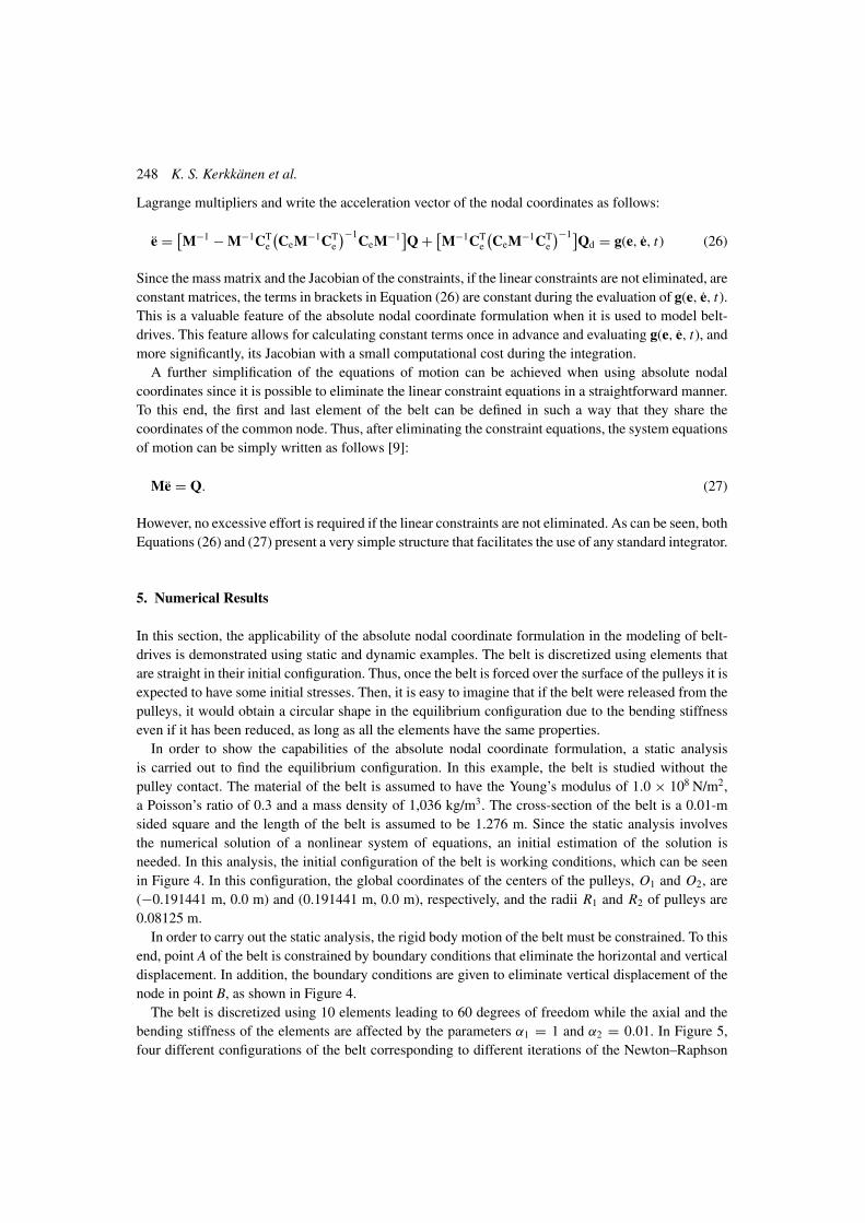
In order to carry out the static analysis, the rigid body motion of the belt must be constrained. To this
end, point A of the belt is constrained by boundary conditions that eliminate the horizontal and vertical
displacement. In addition, the boundary conditions are given to eliminate vertical displacement of the
node in point B, as shown in Figure 4.
The belt is discretized using 10 elements leading to 60 degrees of freedom while the axial and the
bending stiffness of the elements are affected by the parameters α1 = 1 and α2 = 0.01. In Figure 5,
four different configurations of the belt corresponding to different iterations of the Newton–Raphson
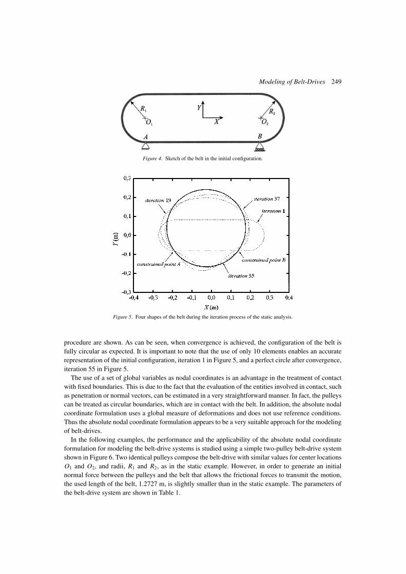
Modeling of Belt-Drives 249
Figure 4. Sketch of the belt in the initial configuration.
Figure 5. Four shapes of the belt during the iteration process of the static analysis.
procedure are shown. As can be seen, when convergence is achieved, the configuration of the belt is
fully circular as expected. It is important to note that the use of only 10 elements enables an accurate
representation of the initial configuration, iteration 1 in Figure 5, and a perfect circle after convergence,
iteration 55 in Figure 5.
The use of a set of global variables as nodal coordinates is an advantage in the treatment of contact
with fixed boundaries. This is due to the fact that the evaluation of the entities involved in contact, such
as penetration or normal vectors, can be estimated in a very straightforward manner. In fact, the pulleys
can be treated as circular boundaries, which are in contact with the belt. In addition, the absolute nodal
coordinate formulation uses a global measure of deformations and does not use reference conditions.
Thus the absolute nodal coordinate formulation appears to be a very suitable approach for the modeling
of belt-drives.
In the following examples, the performance and the applicability of the absolute nodal coordinate
formulation for modeling the belt-drive systems is studied using a simple two-pulley belt-drive system
shown in Figure 6. Two identical pulleys compose the belt-drive with similar values for center locations
O1 and O2, and radii, R1 and R2, as in the static example. However, in order to generate an initial
normal force between the pulleys and the belt that allows the frictional forces to transmit the motion,
the used length of the belt, 1.2727 m, is slightly smaller than in the static example. The parameters of
the belt-drive system are shown in Table 1.
250 K. S. Kerkkanen et al.
Table 1. Parameters of the studied belt-drive system.
Belt-drive parameter Symbol Assigned value
Radius of the driver pulley R1 0.08125 (m)
Radius of the driven pulley R2 0.08125 (m)
Span length L 0.382882 (m)
Coordinates of the center of the driver pulley O1 (−0.191441, 0.0) (m)
Coordinates of the center of the driven pulley O2 (0.191441, 0.0)(m)
Density of the belt material ρ 1036 (kg/m3)
Zero-strain cross-section of the belt A 0.01-m sided square
Young’s modulus E 1.0 × 10⁸ (N/m2)
Poisson’s ratio ν 0.3
Stiffness coefficient of the penalty spring-damper kp 1.0 × 10⁷ (N/m2)
Damping coefficient of the penalty spring-damper cp 1.0 × 101 (Ns/m2)
Friction coefficient between the belt and the pulley μ 1.2
Mass moment of inertia of the driven pulley I 0.1 (kg m2)
Friction creep-rate factor vS 1.0 × 10⁵ (kg/m s)
Axial stiffness parameter α1 1.0
Bending stiffness parameter α2 0.01
Figure 6. Two-pulley belt-drive system.
The driven pulley only has freedom to rotate about its center and the angular velocity of the driver
pulley is subjected to the following velocity profile:
ωdriver =
⎧⎪⎪⎨⎪⎪⎩0, if t ≤ 0.05
12t-0.05
0.6-0.05, if 0.05 < t ≤ 0.6
12, if 0.6 < t
. (28)
Due to Equation (28), the angular velocity of the driver pulley is linearly ramped from 0 to 12 rad/s in
0.55 s. After that, a constant driver pulley angular velocity is maintained until a final simulation time
is reached.
Figure 7 shows the angular velocity of the driver and driven pulleys during the simulation for dis-
cretizations of different number of elements. As can be seen in Figure 7, the results obtained using 20
(120 degrees of freedom), 25 (150 degrees of freedom) and 30 (180 degrees of freedom) elements are
practically equal. This observation indicates that convergence is achieved with a relatively low number
of elements. Based on this result, the model of 20 elements is considered to be accurate enough for this
study and is used in the following examples to introduce some comparisons. Thus, the model uses only
four elements (30 degrees of freedom) to discretize half of the pulley, which is significantly smaller
than the number of elements and degrees of freedom used in the models of Leamy and Wasfy [1, 7].
Modeling of Belt-Drives 251
Figure 7. Angular velocities of the pulleys for different number of elements.
The amplitude of the oscillations of the angular velocity of the driven pulley around the velocity
of the driver pulley can be reduced if the stiffness of the belt is increased as shown in Figure 8. Two
different values of the Young’s modulus, 1.0 × 10⁸ and 1.0 × 10⁹ N/m2, have been used to obtain the
results shown in Figure 8, while the other parameters of the model have not been changed.
Another important parameter of the model is the friction creep-rate factor, vS, since small values
of this parameter lead to a more computationally efficient integration procedure. However, the results
cannot be acceptable for certain values of vS since it may lead to excessive slippage of the belt over the
pulley and even the inability of the model to react to the changes of the angular velocity in the driver
pulley. The results of two simulations using the elements with a Young’s modulus of 1.0 × 10⁹ N/m2
and two different values of vS, 1.0×10⁴ and 1.0×10⁵ kg/m s are shown in Figure 9. As can be observed
from the figure, the smaller value of vS conduces to a delay in the velocity of the driven pulley when
Figure 8. Influence of the stiffness of the belt.
252 K. S. Kerkkanen et al.
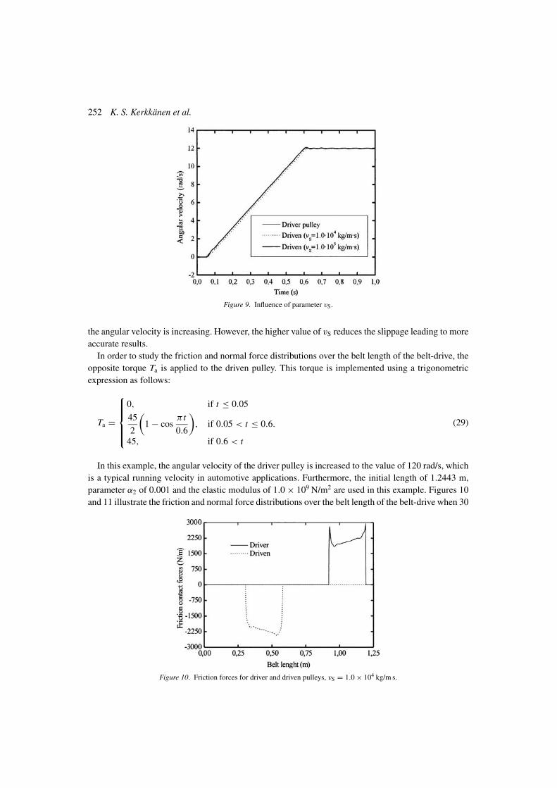
Figure 9. Influence of parameter vS.
the angular velocity is increasing. However, the higher value of vS reduces the slippage leading to more
accurate results.
In order to study the friction and normal force distributions over the belt length of the belt-drive, the
opposite torque Ta is applied to the driven pulley. This torque is implemented using a trigonometric
expression as follows:
Ta =
⎧⎪⎪⎪⎨⎪⎪⎪⎩0, if t ≤ 0.05
45
2
(1 − cos
π t
0.6
), if 0.05 < t ≤ 0.6.
45, if 0.6 < t
(29)
In this example, the angular velocity of the driver pulley is increased to the value of 120 rad/s, which
is a typical running velocity in automotive applications. Furthermore, the initial length of 1.2443 m,
parameter α2 of 0.001 and the elastic modulus of 1.0 × 10⁹ N/m2 are used in this example. Figures 10
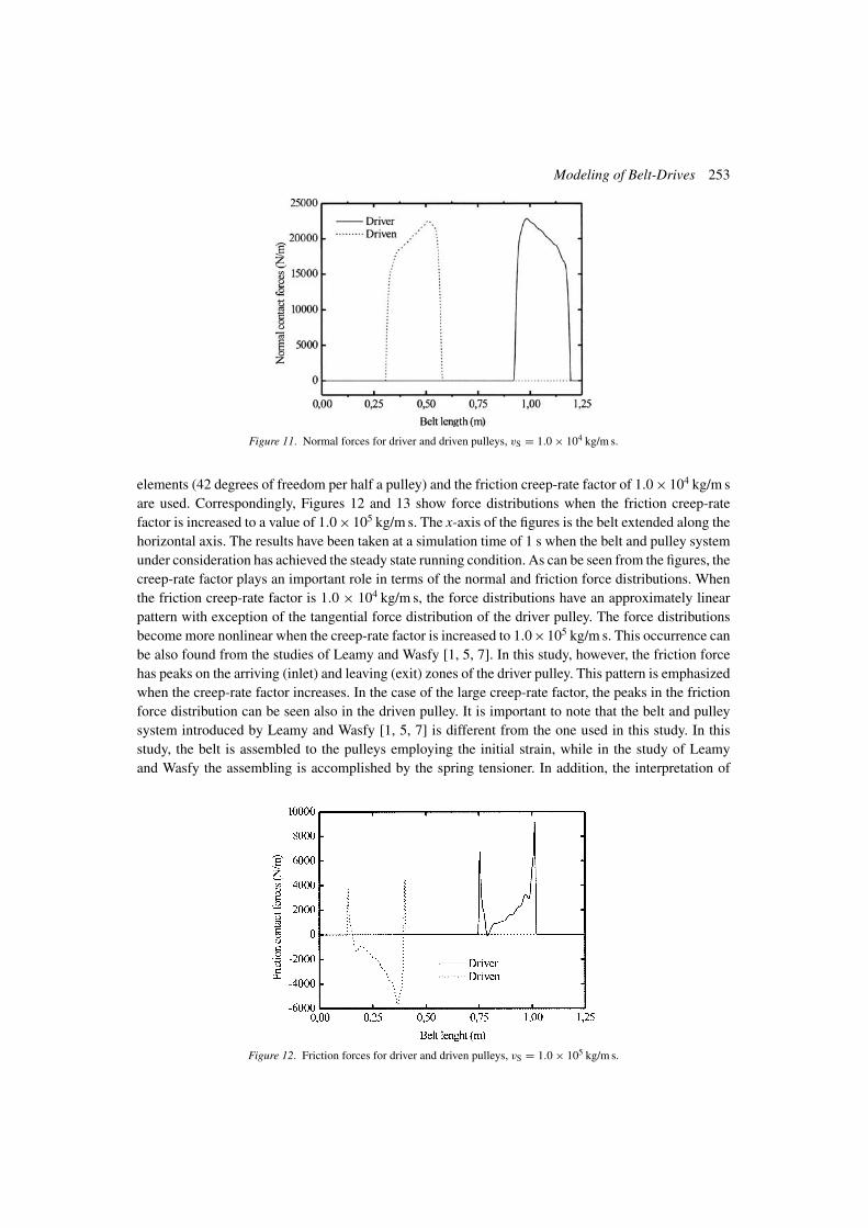
and 11 illustrate the friction and normal force distributions over the belt length of the belt-drive when 30
Figure 10. Friction forces for driver and driven pulleys, vS = 1.0 × 10⁴ kg/m s.
Modeling of Belt-Drives 253
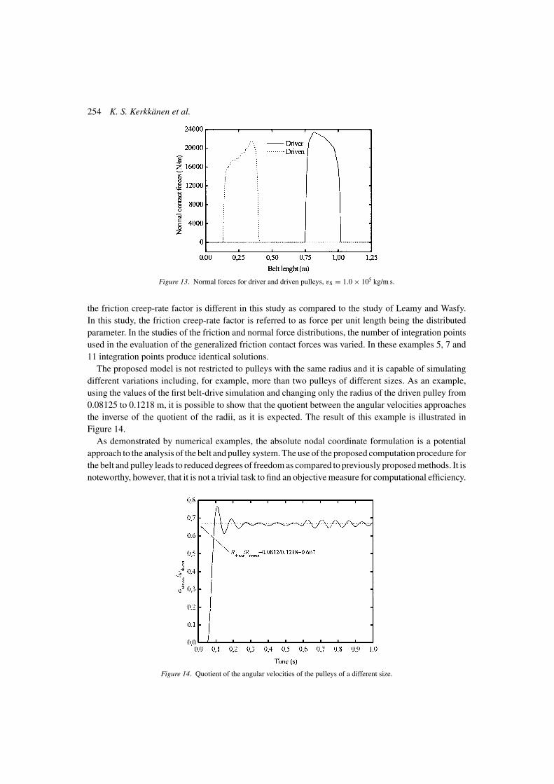
Figure 11. Normal forces for driver and driven pulleys, vS = 1.0 × 10⁴ kg/m s.
elements (42 degrees of freedom per half a pulley) and the friction creep-rate factor of 1.0 × 10⁴ kg/m s
are used. Correspondingly, Figures 12 and 13 show force distributions when the friction creep-rate
factor is increased to a value of 1.0 × 10⁵ kg/m s. The x-axis of the figures is the belt extended along the
horizontal axis. The results have been taken at a simulation time of 1 s when the belt and pulley system
under consideration has achieved the steady state running condition. As can be seen from the figures, the
creep-rate factor plays an important role in terms of the normal and friction force distributions. When
the friction creep-rate factor is 1.0 × 10⁴ kg/m s, the force distributions have an approximately linear
pattern with exception of the tangential force distribution of the driver pulley. The force distributions
become more nonlinear when the creep-rate factor is increased to 1.0×10⁵ kg/m s. This occurrence can
be also found from the studies of Leamy and Wasfy [1, 5, 7]. In this study, however, the friction force
has peaks on the arriving (inlet) and leaving (exit) zones of the driver pulley. This pattern is emphasized
when the creep-rate factor increases. In the case of the large creep-rate factor, the peaks in the friction
force distribution can be seen also in the driven pulley. It is important to note that the belt and pulley
system introduced by Leamy and Wasfy [1, 5, 7] is different from the one used in this study. In this
study, the belt is assembled to the pulleys employing the initial strain, while in the study of Leamy
and Wasfy the assembling is accomplished by the spring tensioner. In addition, the interpretation of
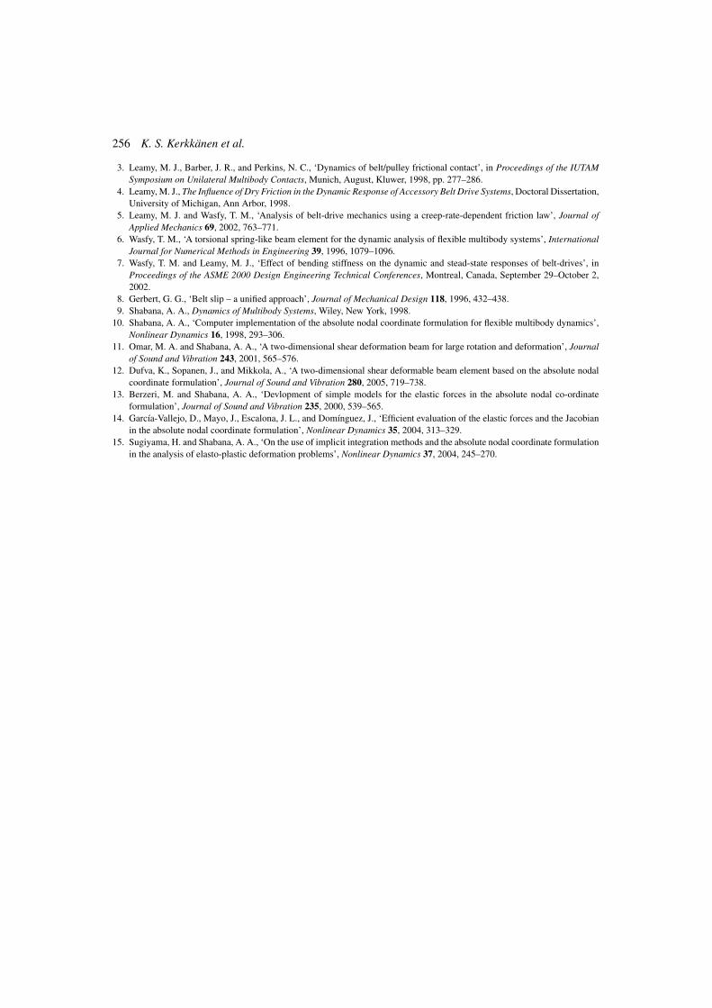
Figure 12. Friction forces for driver and driven pulleys, vS = 1.0 × 10⁵ kg/m s.
254 K. S. Kerkkanen et al.
Figure 13. Normal forces for driver and driven pulleys, vS = 1.0 × 10⁵ kg/m s.
the friction creep-rate factor is different in this study as compared to the study of Leamy and Wasfy.
In this study, the friction creep-rate factor is referred to as force per unit length being the distributed
parameter. In the studies of the friction and normal force distributions, the number of integration points
used in the evaluation of the generalized friction contact forces was varied. In these examples 5, 7 and
11 integration points produce identical solutions.
The proposed model is not restricted to pulleys with the same radius and it is capable of simulating
different variations including, for example, more than two pulleys of different sizes. As an example,
using the values of the first belt-drive simulation and changing only the radius of the driven pulley from
0.08125 to 0.1218 m, it is possible to show that the quotient between the angular velocities approaches
the inverse of the quotient of the radii, as it is expected. The result of this example is illustrated in
Figure 14.
As demonstrated by numerical examples, the absolute nodal coordinate formulation is a potential
approach to the analysis of the belt and pulley system. The use of the proposed computation procedure for
the belt and pulley leads to reduced degrees of freedom as compared to previously proposed methods. It is
noteworthy, however, that it is not a trivial task to find an objective measure for computational efficiency.
Figure 14. Quotient of the angular velocities of the pulleys of a different size.

Modeling of Belt-Drives 255
Even often used CPU time can easily be misleading due to different implementation techniques. In the
case of the absolute nodal coordinate formulation, a number of studies have recently been focused on the
improvement of the numerical performance of the formulation [14, 15]. Utilizing these improvement
proposals, the computer implementation of the absolute nodal coordinate formulation can be carried
out more efficiently in a computational sense.
6. Conclusions
The objective of this study is to find out the applicability of the absolute nodal coordinate formulation
to model the simple belt-drive system. The requirements for the successful and efficient analysis of the
belt-drive system are the exact modeling of the rigid body inertia during an arbitrary rigid body motion,
the consideration of the effect of the shear deformation, the exact description of the highly nonlinear
deformations and a simple and realistic description of the contact. All these requirements are fulfilled
by a recently proposed two-dimensional shear deformable beam element [12]. Based on this element, a
belt-like element has been presented in this paper. The new element allows the user to control the axial
and bending stiffness through the use of two parameters. Thus, the new element is capable of presenting
a very high stiffness in axial solicitation as well as of opposing a small resistance to bending, just as a
piece of a typical belt.
The contact between the belt and the pulleys was modeled using an elastic approach. This procedure
uses the penetration of the belt inside the pulley to calculate the normal and friction forces involved in
contact. Therefore, no constraint equations need to be added to the equations of motion of the system.
Due to the use of high-order elements the contact forces can be distributed along the length of the
element instead of concentrating them at the nodes as it has been done in the literature [1, 5, 7]. With
this contribution to the contact model there is no need to use a high number of nodes for realistic
representation of the boundary of the pulley.
Several numerical examples, including both static and dynamic tests, were used to demonstrate the
functionality and usability of the absolute nodal coordinate formulation in the modeling of the belt-drive
system. The numerical results show that using the distributed contact forces and high-order elements
based on the absolute nodal coordinate formulation, the realistic behavior of the belt-drives can be
obtained with a significantly smaller number of elements and degrees of freedom in comparison to the
previously published finite element models of belt-drives. The results of the examples demonstrate a
good functionality and suitability of the absolute nodal coordinate formulation for the computationally
efficient and realistic modeling of belt-drives.
Acknowledgments
This study was supported by the National Technology Agency in Finland (TEKES) and, in part, by the
Academy of Finland and the Spanish Ministry of Science and Technology.
References
1. Leamy, M. J. and Wasfy, T. M., ‘Transient and steady-state dynamic finite element modeling of belt-drives’, Journal ofDynamic Systems, Measurement and Control 124, 2002, 575–581.
2. Leamy, M. J., Barber, J. R., and Perkins, N. C., ‘Distortion of a harmonic elastic wave reflected from a dry friction support’,
Journal of Applied Mechanics 65, 1998, 851–857.
256 K. S. Kerkkanen et al.
3. Leamy, M. J., Barber, J. R., and Perkins, N. C., ‘Dynamics of belt/pulley frictional contact’, in Proceedings of the IUTAMSymposium on Unilateral Multibody Contacts, Munich, August, Kluwer, 1998, pp. 277–286.
4. Leamy, M. J., The Influence of Dry Friction in the Dynamic Response of Accessory Belt Drive Systems, Doctoral Dissertation,
University of Michigan, Ann Arbor, 1998.
5. Leamy, M. J. and Wasfy, T. M., ‘Analysis of belt-drive mechanics using a creep-rate-dependent friction law’, Journal ofApplied Mechanics 69, 2002, 763–771.
6. Wasfy, T. M., ‘A torsional spring-like beam element for the dynamic analysis of flexible multibody systems’, InternationalJournal for Numerical Methods in Engineering 39, 1996, 1079–1096.
7. Wasfy, T. M. and Leamy, M. J., ‘Effect of bending stiffness on the dynamic and stead-state responses of belt-drives’, in
Proceedings of the ASME 2000 Design Engineering Technical Conferences, Montreal, Canada, September 29–October 2,
2002.
8. Gerbert, G. G., ‘Belt slip – a unified approach’, Journal of Mechanical Design 118, 1996, 432–438.
9. Shabana, A. A., Dynamics of Multibody Systems, Wiley, New York, 1998.
10. Shabana, A. A., ‘Computer implementation of the absolute nodal coordinate formulation for flexible multibody dynamics’,
Nonlinear Dynamics 16, 1998, 293–306.
11. Omar, M. A. and Shabana, A. A., ‘A two-dimensional shear deformation beam for large rotation and deformation’, Journalof Sound and Vibration 243, 2001, 565–576.
12. Dufva, K., Sopanen, J., and Mikkola, A., ‘A two-dimensional shear deformable beam element based on the absolute nodal
coordinate formulation’, Journal of Sound and Vibration 280, 2005, 719–738.
13. Berzeri, M. and Shabana, A. A., ‘Devlopment of simple models for the elastic forces in the absolute nodal co-ordinate
formulation’, Journal of Sound and Vibration 235, 2000, 539–565.
14. Garcıa-Vallejo, D., Mayo, J., Escalona, J. L., and Domınguez, J., ‘Efficient evaluation of the elastic forces and the Jacobian
in the absolute nodal coordinate formulation’, Nonlinear Dynamics 35, 2004, 313–329.
15. Sugiyama, H. and Shabana, A. A., ‘On the use of implicit integration methods and the absolute nodal coordinate formulation
in the analysis of elasto-plastic deformation problems’, Nonlinear Dynamics 37, 2004, 245–270.