Metropolitan Road Traffic Simulation on FPGAs

Justin L. Tripp, Henning S. Mortveit, Anders̊A. Hansson, Maya GokhaleLos Alamos National Laboratory

Los Alamos, NM 87545Email: {jtripp, henning, hansson, maya}@lanl.gov

Abstract

This work demonstrates that road traffic simulation ofentire metropolitan areas is possible with reconfigurablesupercomputing that combines 64-bit microprocessors andFPGAs in a high bandwidth, low latency interconnect. Pre-viously, traffic simulation on FPGAs was limited to veryshort road segments or required a very large number of FP-GAs. Our data streaming approach overcomes scaling is-sues associated with direct implementations and still allowsfor high-level parallelism by dividing the data sets betweenhardware and software across the reconfigurable supercom-puter. Using one FPGA on the Cray XD1 supercomputer,we are able to achieve a 34.4× speed up over the AMD mi-croprocessor. System integration issues must be optimizedto exploit this speedup in the overall simulation.

1. Introduction

Modern society relies on a set of complex, interrelatedand interdependent infrastructures. Over the past ten years,Los Alamos National Laboratory has developed a sophis-ticated suite for simulating various infrastructure compo-nents, such as road networks (TRANSIMS [12]), communi-cation networks (AdHopNet [1]), and the spread of diseasein human populations (EpiSims [6]). These powerful sim-ulation tools can help policy makers understand and ana-lyze interrelated dynamical systems and support decision-making for better planning, monitoring, and proper re-sponse to disruptions. TRANSIMS, for example, can simu-late the traffic of entire cities, with people traveling in carson road networks. It is based on interacting cellular au-tomata (CA), and requires the use of large computer clustersfor efficient computation.

A short description of how TRANSIMS operates is asfollows: First, a syntheticpopulation is created based onsurvey data for the given city. It is created in a such a waythat all statistical quantities and averages considered areconsistent with the survey data. Examples of such quantities

are age distributions, household sizes, income distributions,and car ownership distributions. In the next stage, realistictravel plansare made for all the individuals for a twenty-four hour day. An example plan could be: 1) bring kids toschool, 2) go to work, 3) pick up kids, 4) stop at the grocerystore, 5) drive home. Theroutercoordinates the plans of allindividuals to produce realistictravel routeswith realistictravel times. The router operates together with themicro-simulatorwhich is the module responsible for moving enti-ties around. TRANSIMS uses the actual transportation in-frastructure of the city, so a route could look like: 1) start atA, 2) drive to B, 3) walk to C, 4) take shuttle to D. Furtherinformation can be found at [12] along with descriptions ofa recent study of the Portland metro area. Our FPGA imple-mentation accelerates the micro-simulator and is presentlylimited to cars. The details of the micro-simulator are givenin the next section.

The Portland TRANSIMS study is representative of alarge traffic micro-simulation [2]. The Portland road net-work representation has roughly 124,000 road segmentswith average length about250 meters. Assuming that thereare on average1.5 lanes in each direction on a road seg-ment and using the TRANSIMS standard7.5 meter roadcell length, there are roughly6.25 million road cells. Forcities like Chicago, Houston, and Los Angeles this numberis larger by a factor of3× to 10×.

In this work we study the acceleration of the road net-work simulation through an FPGA implementation. Sincethe simulation is parallel, with independent agents thatmake decisions based on local knowledge, it seems natu-ral to map to the large-scale spatial parallelism offered byFPGAs. The high degree of regularity found in the roadnetwork is another reason that this application is well suitedapplication to FPGAs. In contrast, other networks such asad hoc wireless communication networks or social contactnetworks relevant for transmission of contagious disease aremuch more irregular and dynamic.

2. Related Work

FPGAs have previously been applied to the traffic sim-ulation problem. The earliest system, by George Milne[7, 11], simulated road networks by directly implementingtheir behavior in hardware. Milne’s direct implementationuses Algotronix’s CAL FPGAs to create a long single-laneroad of traffic. The cars can be placed on the road and theirbehavior with respect to each other simulated. Results ofthe simulation are obtained using read-back from each ofthe chips used in the simulation. Cars were able to have twospeeds (go/stop) and their behavior was determined basedon the presence of their nearest neighbor. The direct imple-mentation approach has a very high degree of concurrencythat is limited by the amount of hardware available and thelevel of data visibility required by the simulation.

A more recent system, by Marc Bumble [3], implementsa generalized system for parallel event-driven simulation.His system consists of an event generator, an event queue, ascheduler, and a unifying communications network in eachprocessing element. Each of the processing elements canbe built in reconfigurable hardware at a cost of 30–34 Al-tera Apex FPGAs. The traffic simulation is calculated bystreaming data into processing elements. Each processingelement is capable of simulating one source, intersection,or destination node with the associated outbound roads oftraffic. Bumble states that a system composed of 8000 pro-cessing elements could simulate a large traffic network (at acost of 240,000 FPGAs).

Bumble does not address the scalability of his approach,the visibility of the simulated traffic or how data is trans-fered in and out of the system. Also, his road modelsare limited to single-lanes with simple four-way intersec-tions. This approach does not lend itself to the simulationof metropolitan areas.

The work presented here differs from previous ap-proaches in three ways. First, we are using simulation mod-els which are currently in production use. TRANSIMSmodels include acceleration, stochastic slow-down, differ-ent velocities and cars with routes. Second, we extend oursimulation to entire metropolitan areas rather than special-ized configuration with a small number roads and intersec-tions. Previously, the cost of metropolitan scale traffic sim-ulations solely on FPGAs was too expensive, so as a thirdpoint we will examine the cost of partitioning the simulationbetween the microprocessors and FPGA. All of these differ-ences help determine the utility of FPGAs in the context oflarge-scale simulations such as TRANSIMS.

3. CA Traffic Modeling

The TRANSIMS road network simulator, which is basedon [8–10], can best be described as a cellular automaton

computation on a semi-regular grid or cell network: Therepresentation of the city road network is split into nodesand links. Nodes correspond to locations where there isa change in the road network such as an intersection or alane merging point. Nodes are connected by links that con-sist of one or more unidirectional lanes (see Figure 3). Alane is divided into road cells each of which are7.5 meterslong. One cell can hold at most one car, and a car can travelwith velocity v ∈ {0, 1, 2, 3, 4, 5} cells per iteration step.The positions of the cars are updated once every iterationstep using a synchronous update, and each iteration step ad-vances the global time by one second. The basic driving

Figure 1. CA traffic in TRANSIMS

rules for multi-lane traffic in TRANSIMS can be describedby a four-step algorithm. In each step we consider a singlecell i in a given lane and link. Note that our model allowspassing on the left and the right. To avoid cars merging intothe same lane, cars may only change lanes to the left on oddtime steps and to the right on even time steps. This conven-tion, along with the four algorithm steps described below,produces realistic traffic flows as demonstrated by TRAN-SIMS.

3.1. Local driving rules

The micro-simulator has four basic driving rules. Welet ∆(i) andδ(i) denote the cell gap in front of celli andbehind celli, respectively.v is the velocity of the car in celli andvmax(i) is the maximum velocity for this particularroad cell, which may be lower than the globalvmax (e.g., alocal speed limit).

1. Lane Change Decision:Odd time stept: If cell i has acar and a left lane change isdesirable(car can go fasterin target lane) andpermissible(there is space for a safelane change) flag the car/cell for a left lane change.The case of even numbered time steps is analogous. Ifthe cell is empty nothing is done.

2. Lane Change:Odd time stept: If there is a car in celli,and this car is flagged for a left lane change then clearcell i. Otherwise, if there is no car in celli and if theright neighbor of celli is flagged for a left lane change

2

then move the car from the neighbor cell to celli. Thecase of even time stepst is analogous.

3. Velocity Update:Each celli that has a car updates thatcar’s velocity using the two-step sequence:

• vnext := min(v + 1, vmax(i),∆(i)) (accelera-tion)

• If [UniformRandom() < pbreak] and[v > 0]thenvnext := v − 1 (stochastic deceleration).

4. Position Update:If there is a car in celli with velocityv = 0, do nothing. If celli has a car withv > 0 thenclear celli. Else, if there is a carδ(i) + 1 cells behindcell i and the velocity of this car isδ(i) + 1 then movethis car to celli. The nature of the previous velocityupdate pass guarantees that there will be no collisions.

All cells in a road network are updated simultaneously. Thesteps 1–4 are performed for each road cell in the sequencethey appear. Each step above is thus a classical cellular au-tomatonΦi. The whole combined update pass is a productCA, that is, a functional composition of classical CAs:

Φ = Φ4 ◦ Φ3 ◦ Φ2 ◦ Φ1

Note that the CAs used for the lane change and the velocityupdate are stochastic CAs. The rationale for having stochas-tic braking is that it produces more realistic traffic. The factthat lane changes are done with a certain probability avoidsslamming behavior where whole rows of cars change lanesin complete synchrony.

3.2. Intersections and Global Behavior

The four basic rules handle the case of straight roadways.TRANSIMS uses travel routes to generate realistic trafficfrom a global point of view. Each traveler or car is assigneda route that he/she has to follow. Routes mainly affect thedynamics near turn-lanes and before intersections as carsneed to get into a lane that will allow them to perform thedesired turns.

To incorporate routes the road links need to have IDsassigned to them. Moreover, to keep computations as localas possible, cells need to hold information about the IDs ofupcoming left and right turns.

The following describes the extension of the four basicdriver rules to handle turn-lanes and intersections.

Modification of the lane change rule:

We consider a car in celli. As before, lane changes to theleft/right are only permissible on odd/even numbered timesteps. We refer to the adjacent candidate cell as the targetcell.

1. If the link ID of the target cell matches the next leg ofthe travel route and differs from the current link ID, alane change is desirable (desirable turn-lane).

2. Else, if the target cell has a link ID that does not matchthe next leg of the route and it differs from the cur-rent link ID of the route, a lane change is not desirable(wrong turn).

3. Else, if the current cell’s nextLeftLink (nextRightLink)ID matches the next leg of the route and the simulationtime is an odd (even) integer, a lane change is desirable(prepare for turn-lane or intersection).

4. Else, apply the basic lane changing rule describedabove.

Note that this handles lane changing prior to turn-lanesas well as intersections.

Intersection Logic

An intersection has a number of incoming and outgoinglinks associated with it. A simplified set of turning rules(assuming a four-way intersection) are as follows:

1. Only cars in an incoming left(right)-most lane of linkcan turn left(right). A car that turns left(right) mustinitially use the left(right)-most lane of the target link.

2. A car in any incoming lane can go straight. A car thatgoes straight must use the same lane number in the tar-get link as it used in the incoming link. It is assumedthat the lane counts for the relevant links agree.

More intricate intersection geometries can, of course, occurbut the basic idea remains the same. When intersections areclose it is natural to modify the first rule: when a left turnis followed by an immediate right turn the rightmost lane ischosen as target lane for the left turn.

An intersection has a set of immediate adjacent roadcells. We refer to these as theintersection road cells. Theintersections operate by dynamically assigning the front andback neighbor cell IDs of the intersection road cells. Thisallows us to naturally extend the driving rules for multi-lanetraffic to intersections without any modifications. The sub-set of the intersection road cells that come from incominglinks have their front neighbor cell set to zero by default.The same holds for the back neighbor of the intersectioncells belonging to outgoing links. The intersections operateby establishing front/back pairs between cells to accommo-date the routes. Stop intersections and traffic signal inter-sections impose additional constraints on which cars are al-lowed to drive at what times by controlling the correspond-ing connections.

3

Link

NodeMerge

IntersectionNode

Road Cell

VelocityUpdate

LaneChange

Random 5 Cell Neighbor Info

NeighborInfo

State

StateMachine

State Id

Computation Engine

NeighborInfo

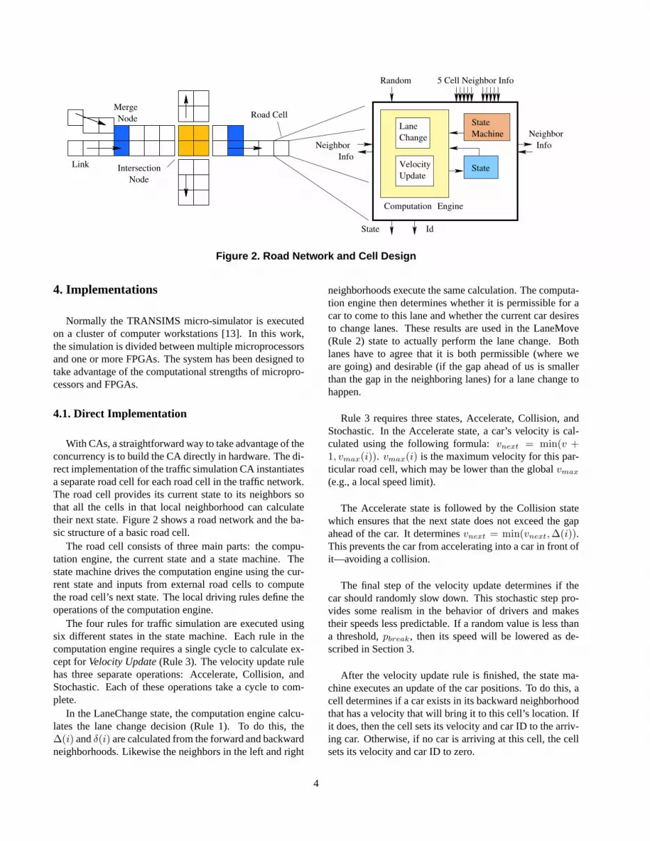
Figure 2. Road Network and Cell Design

4. Implementations

Normally the TRANSIMS micro-simulator is executedon a cluster of computer workstations [13]. In this work,the simulation is divided between multiple microprocessorsand one or more FPGAs. The system has been designed totake advantage of the computational strengths of micropro-cessors and FPGAs.

4.1. Direct Implementation

With CAs, a straightforward way to take advantage of theconcurrency is to build the CA directly in hardware. The di-rect implementation of the traffic simulation CA instantiatesa separate road cell for each road cell in the traffic network.The road cell provides its current state to its neighbors sothat all the cells in that local neighborhood can calculatetheir next state. Figure 2 shows a road network and the ba-sic structure of a basic road cell.

The road cell consists of three main parts: the compu-tation engine, the current state and a state machine. Thestate machine drives the computation engine using the cur-rent state and inputs from external road cells to computethe road cell’s next state. The local driving rules define theoperations of the computation engine.

The four rules for traffic simulation are executed usingsix different states in the state machine. Each rule in thecomputation engine requires a single cycle to calculate ex-cept forVelocity Update(Rule 3). The velocity update rulehas three separate operations: Accelerate, Collision, andStochastic. Each of these operations take a cycle to com-plete.

In the LaneChange state, the computation engine calcu-lates the lane change decision (Rule 1). To do this, the∆(i) andδ(i) are calculated from the forward and backwardneighborhoods. Likewise the neighbors in the left and right

neighborhoods execute the same calculation. The computa-tion engine then determines whether it is permissible for acar to come to this lane and whether the current car desiresto change lanes. These results are used in the LaneMove(Rule 2) state to actually perform the lane change. Bothlanes have to agree that it is both permissible (where weare going) and desirable (if the gap ahead of us is smallerthan the gap in the neighboring lanes) for a lane change tohappen.

Rule 3 requires three states, Accelerate, Collision, andStochastic. In the Accelerate state, a car’s velocity is cal-culated using the following formula:vnext = min(v +1, vmax(i)). vmax(i) is the maximum velocity for this par-ticular road cell, which may be lower than the globalvmax

(e.g., a local speed limit).

The Accelerate state is followed by the Collision statewhich ensures that the next state does not exceed the gapahead of the car. It determinesvnext = min(vnext,∆(i)).This prevents the car from accelerating into a car in front ofit—avoiding a collision.

The final step of the velocity update determines if thecar should randomly slow down. This stochastic step pro-vides some realism in the behavior of drivers and makestheir speeds less predictable. If a random value is less thana threshold,pbreak, then its speed will be lowered as de-scribed in Section 3.

After the velocity update rule is finished, the state ma-chine executes an update of the car positions. To do this, acell determines if a car exists in its backward neighborhoodthat has a velocity that will bring it to this cell’s location. Ifit does, then the cell sets its velocity and car ID to the arriv-ing car. Otherwise, if no car is arriving at this cell, the cellsets its velocity and car ID to zero.

4

4.2 A Scalable Approach

A common approach used on FPGAs in many appli-cations (like DSP) is to stream data through a number ofcomputational units. In the context of traffic simulation,streaming can be achieved through acomputation enginethat processes a stream of road data and subsequently out-puts a stream of updated data. Thus, the number of roadcells are no longer limited to available FPGA area. Instead,the only limiting factor is the size of the memory to holdthe state of the road cells and the associated access time.Thus, a streaming hardware design becomes scalable andcan handle large-scale road networks.

In our streaming design, we partition the road network insuch a way that straight road sections are processed by thehardware, while intersections and merging nodes are up-dated by a software module. Most importantly, this hybridhardware/software strategy means that hardware processingis governed by a simple, homogeneous set of traffic rules,while all road plan decisions are handled by software.

traffic flow update direction

overlap region II overlap region I

Figure 3. Road Link Structure.

The data representing straight lanes is fed to the hard-ware update engine against the flow of traffic, starting fromthe end of each lane. However, due to the partitioning ofthe road network, the cars in the lastvmax cells of each lanecannot be updated since the engine lacks knowledge aboutthe network topology and the road plans. For this reason wedefine anoverlap region I(see Figure 3), which is the lastvmax cells of each lane, and because of the processing di-rection of the computation engine, these cells are processedfirst. Although cars that are inside an overlap region at thebeginning of the hardware computation cannot be updatedby the engine, it is important to note that the engine canmove other carsinto these first cells during its computa-tional pass. Naturally, the software module needs to updatethe position and velocity of cars inside the overlap regionsat the end of each hardware update pass.

The software must also write information to the firstvmax cells of each lane, which corresponds to new carsmoving into a lane (arriving from other lanes, either throughan intersection or by merging). However, computing ve-locities and positions of these new cars requires completeknowledge of the firstvmax cells of each lane. In a sense,the firstvmax cells of each lane then constitute another over-lap region (see overlap region II in Figure 3) that needs to

be touched by software at the end of each pass. However,the hardware can only move carsfrom these first cells, andif the cells were empty at the beginning of the update pass,the software module does not need to read back the updatedstatus. Also, in order to minimize the cost of memory syn-chronization, we have chosen to process only single-lanetraffic in hardware.1 In fact, 90% of all roads in Portlandare one-lane roads, which means that most road cells arestill updated in hardware.

The hardware design, shown in Figure 4 implements amemory interface, whose main responsibility is to generateread and write addresses used for accessing the memories.Both the read and write addresses are generated by counters.The counter associated with the read starts from the lowestaddress each new time the computation engine is requestedto process data, and it continues to count until the softwaremodule schedules a new update request. The counter asso-ciated with the write address, on the other hand, monitors astatus signal provided by the computation engine, and stopscounting as soon as the engine signals it is done.

Update engine

Read Write

MemoryMemory

Addr_genAddr_gen

Enable

Figure 4. Structure of a straightforwardstreaming implementation.

Inside the compute engine, the car’s velocity is updatedfirst, and then its position. Of course, if no car exists in theincoming road cell, or if the incoming road cell belongs toan overlap region, the incoming velocity is passed out un-changed. In all other cases, the engine initially tests whetheran acceleration is permissible. There is also a probabilityof stochastic deceleration. A car slows down if a pseudo-random number is less than a predefined threshold value,pbreak.2 In order to test for acceleration permissibility, in-coming cars are streamed into a shift register, and this reg-

1Clearly, multiple-lane traffic requires overlap regions longer thanvmax cells since the lane changing rules assume knowledge of precedingcells. Only succeeding cell information is needed for single-lane traffic.

2The random number is internally generated by a standard 32-bit linearfeedback shift register.

5

ister is scanned to find the maximum number of cells a carcan move ahead.

Scancellsandoutput

Velocityupdate

Shift register

Figure 5. The Position Update

The streaming engine calculates a car’s position by shift-ing the car one cell every clock cycle (see Figure 5) untilits newly calculated velocity matches the distance from theend of the shift register, which isvmax +1 cells long. At thepoint when there is a match, the change state block exportsall car information to the destination road cell. This pipelin-ing design makes it possible for the computation engine toread and write one word of road data every clock cycle. Ifwe have access toN concurrent memories, it would be ad-vantageous to instantiateN parallel replicas of the computeengine.

5. Using the Cray XD1

The Cray XD1 supercomputer combines high perfor-mance microprocessors, a high speed, low latency intercon-nect network, and reconfigurable computing elements. Thisprovides an environment where data transfer latencies andbandwidth associated with I/O busses is greatly reduced.The tight integration of processors and reconfigurable com-puting changes the meaning of reconfigurable supercomput-ing. A supercomputing problem can be split between theCPU and FPGA with close synchronization and fast com-munication between software and hardware.

5.1. Machine Description

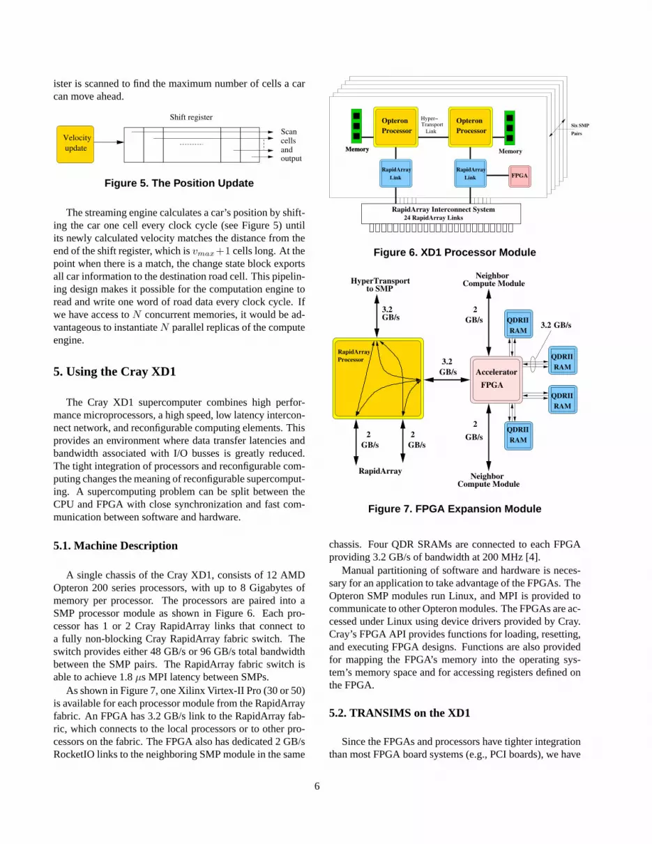
A single chassis of the Cray XD1, consists of 12 AMDOpteron 200 series processors, with up to 8 Gigabytes ofmemory per processor. The processors are paired into aSMP processor module as shown in Figure 6. Each pro-cessor has 1 or 2 Cray RapidArray links that connect toa fully non-blocking Cray RapidArray fabric switch. Theswitch provides either 48 GB/s or 96 GB/s total bandwidthbetween the SMP pairs. The RapidArray fabric switch isable to achieve 1.8µs MPI latency between SMPs.

As shown in Figure 7, one Xilinx Virtex-II Pro (30 or 50)is available for each processor module from the RapidArrayfabric. An FPGA has 3.2 GB/s link to the RapidArray fab-ric, which connects to the local processors or to other pro-cessors on the fabric. The FPGA also has dedicated 2 GB/sRocketIO links to the neighboring SMP module in the same

MemoryMemory Memory

Six SMP

Pairs

FPGA

Hyper−Transport

Link

RapidArray Interconnect System24 RapidArray Links

RapidArrayRapidArray

OpteronProcessor

OpteronProcessor

Link Link

Figure 6. XD1 Processor Module

RapidArray

2GB/s

2GB/s

2GB/s

2GB/s

QDRIIRAM

HyperTransportto SMP

3.2GB/s

3.2GB/s

NeighborCompute Module

NeighborCompute Module

QDRII

QDRII

QDRII

RAM

RAM

RAM

FPGAAccelerator

3.2 GB/s

RapidArrayProcessor

Figure 7. FPGA Expansion Module

chassis. Four QDR SRAMs are connected to each FPGAproviding 3.2 GB/s of bandwidth at 200 MHz [4].

Manual partitioning of software and hardware is neces-sary for an application to take advantage of the FPGAs. TheOpteron SMP modules run Linux, and MPI is provided tocommunicate to other Opteron modules. The FPGAs are ac-cessed under Linux using device drivers provided by Cray.Cray’s FPGA API provides functions for loading, resetting,and executing FPGA designs. Functions are also providedfor mapping the FPGA’s memory into the operating sys-tem’s memory space and for accessing registers defined onthe FPGA.

5.2. TRANSIMS on the XD1

Since the FPGAs and processors have tighter integrationthan most FPGA board systems (e.g., PCI boards), we have

6

partitioned the road traffic simulation between the FPGAand CPUs available in the system. Single-lane roads makeup 90% of the road segments in the Portland network. TheFPGAs are tailored to process single-lane traffic. The CPUsin the XD1 are responsible for data synchronization be-tween the hardware and the software, and simulating mul-tiple lanes and intersections. Based on the size of the datarequired, two FPGA nodes are needed for simulation so thatall of Portland can fit in the memories available.

The implementation on the XD1 is an improvement overour earlier Osiris based design [14] due in part to betterbandwidth between the memories and the FPGA. The QDRSRAMs on the XD1 are fully dual ported and allow for si-multaneous reads and writes to any memory location. Thisprovides a large amount of external memory bandwidth tothe FPGA.

Despite the large amount of bandwidth on the RapidAr-ray network between the FPGA and the Opteron CPUs, thesimulation attempts to reduce the required amount of datatraffic. Synchronization of data only occurs if there arecars on a particular road segment and only in the overlap(shared) data regions. This allows for better trade-off be-tween calculation and available bandwidth.

5.3. XD1 Communication Costs

As described in theXD1 FPGA Developmentmanual [5],there are asymmetric costs associated with reads and writesbetween the host and the FPGA’s QDR SRAMs. Writes cantake advantage of write combining in the Linux kernel andare non-blocking. On the other hand, reads are blockingand cannot be combined. This creates an asymmetric costwhich must be overcome.

RapidArrayProc.

QDRCore QDR

Memory

Write Ctrl

Write

Read

RT

Core

FPGA

To CPU

FabricArray

RapidTo

EngineTraffic

Figure 8. Default FPGA QDR SRAM access(only one memory shown).

The method for accessing the FPGA’s SRAMs is shownin Figure 8. The multiplexor (mux) between the traffic en-gine and the RapidArray Transport (RT) core allows both

the host and the traffic engine to write to the SRAMs. Readsdo not require a mux for the data, but both read and writerequire muxes for the address lines (not shown). Using thissetup we benchmarked reads and writes from the host to theFPGA.

Table 1. Read and Write Bandwidth (MB/s) forHosts to QDR SRAMS

Array Pointer MemcpyRead 5.94 5.95 6.01Write 1260 1320 1320

Table 1 shows the bandwidth results for reads and writesaccomplished using three different approaches. The FPGASRAMs are mapped into the hosts local memory and canbe accessed using arrays with indexes, using pointers, or byusing thememcpyfunction call. Array accesses were foundto be slight slower, but the bandwidth is roughly equivalent.However, the difference in cost between reads and writes isa factor of200. This asymmetric cost is overcome by usinga “write-only” architecture as suggested by Cray. The hostmust write data to the FPGA memory and the FPGA mustwrite the data that the host needs to read.

TrafficEngine

TrafficEngine

TrafficEngine

EngineTraffic

RoundRobin

RapidArrayFabric

RTCore

Fifos

DataPush

Mux

Figure 9. FPGA Push to write data to theOpteron host.

Figure 9 details the hardware added to the traffic designto make it a write-only architecture. Only cars in overlap ar-eas are transferred to the host. These overlap cars are storedin FIFOs since they can arrive in bursts of up to ten cars.3

The number of cars in overlap areas is dependent on thetraffic data in the memories, so a data push process watcheseach of the FIFOs through a mux that is rotating through theFIFOs in a round-robin fashion. When the data push processsees a FIFO with data in, it stops the round-robin controland sends up to four data words to the host (due to Hyper-Transport requirements). Finally, after sending the data the

3Bursts of ten cars can occur from overlap region 2 of the previous linkbeing adjacent to overlap region 1 of the next link.

7

round robin control moves the mux to the next FIFO. In-dependent of the data push, if a FIFO becomes full it willdisable its traffic engine until the FIFO is empty again.

Use of the FPGA data push process allows the traffic de-sign to reduce the time required to transmit the overlap dataupdates between the FPGA and the host. This allows moretime on the processor and FPGA to be spent processing datainstead of communicating.

6. Results

The results for two different implementations of roadtraffic simulation are presented here. The first, direct im-plementation, creates a physical circuit for each road cellto be simulated. The second, streaming implementation,creates a small number of parallel engines and the data isstreamed through in time. The two implementations repre-sent extremes in concurrency and scalability.

6.1. Direct Implementation

The direct implementation was written in VHDL andsynthesized to EDIF using Synplify v7.6. The EDIF de-scription was passed into Xilinx ISE v6.2 to produce theresults reported.

The results for the direct implementation for multi- andsingle-lane circular traffic are described in Table 2. Thehardware implementation of single-lane traffic has only fourstates, since single-lanes do not require the extra hardwarefor lane changes. The two-lane implementation that in-cludes the hardware to perform lane changes is 63% largerin area. As the table shows, both Xilinx chips can hold (atleast) 400 road cells.

Table 2. Direct Implementation Design Re-sults

One-lane Two-laneV2-6k V2p100 V2-6k V2p100

Cells 650 650 400 640LUTs/Cell 104 97 169 128Clock(MHz) 48.68 64.17 35.53 62.8Slices 33790 31576 33790 40973(% of Slices) (99%) (71%) (99%) (92%)

Table 3 compares the results for the two-lane traffic im-plementation achieved by the Xilinx XC2V6000 (V2-6k)and the XC2VP100 (V2p100) to a software implementationrunning on a 2.2 GHz Opteron processor. The V2-6k sim-ulates the road cells at a rate415.8× the Opteron and theV2p100 simulates traffic just short of1175×. This speedup

comes primarily from the fact that the FPGA implementa-tion is executing all cells concurrently, and the software im-plementation, which may have instruction level parallelism,calculates each cell individually.

Table 3. Direct Implementation Results Com-parison for Two Lanes

2.2GHzV2-6k V2p100 Opteron

Cells 400 640 2 MillionCells/sec 2.37× 109 6.70× 109 5.7× 106

Speedup 415.8 1175.4 1.0

Despite the large speedup that is possible using the directimplementation, the FPGA can only handle a small numberof road cells. Using the data from the Portland TRANSIMSstudy, we know that there are roughly6.6 million road cells.Simulating Portland would require at least 12,400 FPGAsto simulate the entire city. Also, the direct implementationdoes not provide high visibility to the simulation data.

6.2. Streaming Implementation

The streaming implementation was written in VHDL andplaced in VHDL interfaces provided by Cray for the Rap-idArray and QDR SRAMS (release 1.1). All of this wassynthesized using Xilinx XST and the bitstream generatedby Xilinx ISE v6.2.

Table 4. Comparison of Streaming with Soft-ware Simulation

2.2GHzV2p50 Opteron

Slices 1857Clock(MHz) 180 2199Cells/sec 7.2× 108 5.7× 106

Speedup 126.3 1.0

The results shown in Table 4 were timed using a timerregister, called the Time Stamp Counter (TSC), which mea-sures processor ticks at the processor clock rate. The 64-bit read-only counter is extremely accurate, as it is imple-mented as a Model-Specific Register, inside the CPU. Theoverhead of using this register is extremely low and the TSCregister on the 2.2GHz Opteron has a resolution of 450 pi-coseconds.

The design on the FPGA includes four streaming engines(limited by the number of available memories) and operatesat a rate126.3× the speed of a comparable software version

8

running on a 2.2 GHz Opteron. Table 5 shows a more accu-rate speedup which includes the cost of transferring data toand from the FPGAs. If results calculated by the FPGA areread directly by the host, the speed up is only4.5×. This isdue to the blocking nature of reads from the host. Pushingthe results up to the host, as described in Section 5.3, resultsin a more impressive speedup of34.4×.

Although the streaming implementation is a factor of 30slower than the direct approach, it is still enough of an im-provement to provide significant overall speedup. Addi-tional speedup is still possible with more FPGA boards. Themost crucial limiting factor in this implementation is thenumber of memory banks on each board; additional bankswould allow us to increase the number of simultaneous datastreams. In fact, with the current design, one compute en-gine requires less than 5% of chip area. Since each computenode has four concurrent memories, it is advantageous to in-stantiate four parallel engines, but already at this moderatelevel of parallelism, we run into a bandwidth bottleneck.

The hardware performs extremely well with the straightlane segments, which make up 70–90% of the road seg-ments in a given simulation. FPGA aided simulation donein the scalable, streaming approach may be the fastest wayto do extremely large metro-area traffic simulations, espe-cially in light of the advances being made in combined mi-croprocessor/FPGA computing systems. The cellular na-ture of the road segments meshes well with hardware, and acombined hardware/software approach for the full-fledgedsimulation fits each of their computational strengths.

Table 5. Comparison of Streaming includingCommunication Costs

w/o Push Push 2.2GHzV2p50 V2p50 Opteron

Cells/sec 2.56× 107 1.96× 108 5.7× 106

Speedup 4.5 34.4 1.0

6.3. System Integration Issues

We will now discuss costs associated with integrating theFPGA computation engine with the microprocessor and itssoftware environment, and how a realistic road network de-scription of Portland affects this integration.

A profile of the software execution time is shown in Ta-ble 6. The transaction cost of transferring data from theFPGA hardware to the software by having the micropro-cessor read the FPGA memory proved to be unacceptablylong—12.3% of the overall execution time of one simula-tion step. As a remedy for this problem, we implementeda push back mechanism (Section 5.3) in which the FPGA

writes back data to a memory space that is local to the host.This solution led to a hybrid design where the communica-tion time for data transfer is negligible (see Table 6).

Another bottleneck is the size of the FPGA memory. Outof 6.6 million road cells, the 16 MB available FPGA mem-ory can only hold 2 million cells, assuming that 64 bits areused to describe the status of each road cell. If the memorieswere deeper, it would be possible to off-load significantlymore of the overall computation to the FPGA.

We are currently investigating two alternatives to gettingmore road cells processed by hardware: (i) a more succinctrepresentation using only 32 bits instead of 64, and (ii) on-line FPGA data compression. As already explained, thesoftware is responsible for putting new cars in each single-lane road segment (corresponding to cars coming from adja-cent segments). By also keeping track of the order in whichthese new cars enter each segment, we would not have to en-code and send along any car IDs, since cars obviously haveto leave a single-lane road segment in the order in whichthey enter. This implicit road ID method would reduce thesize of a road cell to 32 bits.

To do compression, the FPGA could compress thedata written by the microprocessor using a simple on-linescheme such as run-length encoding. This is possible be-cause the data written by the microprocessor must first gothrough the FPGA. We could also use more aggressive com-pression techniques by exploiting the semantics of the traf-fic data.

Table 6. Percentage of Overall Execution Timeof one Simulation Step

Without push With pushNetwork state update 8.3% 9.7%Software to hardware 0.2% 0.18%Intersections 14.0% 13.8%Lane change update 13.3% 16.8%Velocity update 21.9% 25.5%Position update 30.0% 33.8%Hardware to software 12.3% 0.14%

7. Conclusion and Future Work

In this paper, we investigated hardware acceleration ofthe TRANSIMS road traffic simulator. Using a structuralapproach yields an upper bound on the potential speedup.For straight road segments, this speedup is as high as1175,under the assumption of no communication cost and usinga single FPGA. In comparison, the more scalable stream-ing implementation achieves126× speedup, which was ob-tained for a very simple network topology, excluding in-

9

tersections. In order to handle complex network topolo-gies, we relied on the hybrid nature of the Cray XD1, i.e.,we partitioned the road network such that intersections andmultiple lanes were processed by a software module, whilestraight road sections were processed by the FPGA. Our ap-proach exploits the low latency, high bandwidth intercon-nect network of the Cray XD1 to partition the the prob-lem between software and hardware. For a realistic roaddescription of Portland, we were able to achieve34.4×speedup.

The next step with accelerating this TRANSIMS simu-lation is to add one or more SMP modules to the systemand determine the cost of synchronizing data communica-tion over MPI. It may also be possible to have a single SMPmodule communicate to the other FPGAs via the RapidAr-ray Fabric. The Cray XD1 system provides an interestingtestbed for reconfigurable supercomputing applications.

Acceleration of TRANSIMS opens the door to a wholerange of simulations where FPGAs or other dedicated hard-ware can provide computational speedup. Many simulationsystems today, have a similar structure to the one found inTRANSIMS: there are highly complex computations bestsuited for software and a large collection of structured sim-ple calculations as in the road network simulator. TheTRANSIMS accelerator provides a prime example of howFPGAs can aid a large class of large-scale simulations.

References

[1] K. A. Atkins, C. L. Barret, R. J. Beckman, S. G. Eubank,N. W. Hengarter, G. Istrate, A. V. S. Kumar, M. V. Marathe,H. S. Mortveit, C. M. Reidys, P. R. Romero, R. A. Pistone,J. P. Smith, P. E. Stretz, C. D. Engelhart, M. Droza, M. M.Morin, S. S. Pathak, S. Zust, and S. S. Ravi. ADHOPNET:Integrated tools for end-to-end analysis of extremely largenext generation telecommunication networks. Technical re-port, Los Alamos National Laboratory, Los Alamos, NM,2003.

[2] C. L. Barrett, R. J. Beckman, K. P. Berkbigler, K. R. Bisset,B. W. Bush, K. Campbell, S. Eubank, K. M. Henson, J. M.Hurford, D. A. Kubicek, M. V. Marathe, P. R. Romero, J. P.Smith, L. L. Smith, P. E. Stretz, G. L. Thayer, E. Van Eeck-hout, and M. D. Williams. TRansportation ANalysis SIMu-lation system (TRANSIMS) portland study reports. Decem-ber 2002.

[3] M. D. Bumble. A Parallel Architecture for Non-deterministic Discrete Event Simulation. PhD thesis, Penn-sylvania State University, 2001.

[4] Cray Inc., Seattle, WA.Cray XD1 Datasheet, September2004.

[5] Cray, Inc., Seattle, WA. Cray XD1 FPGA Development,2004.

[6] S. Eubank, H. Guclu, V. S. A. Kumar, M. V.Madhav,A. Srinivasan, Z. Toroczkai, and N. Wang. Modelling dis-ease outbreaks in realistic urban social networks.Nature,429(6988):180–184, May 13, 2004.

[7] G. Milne, P. Cockshott, G. McCaskill, and P. Barrie. Re-alising massively concurrent systems on the space machine.In K. Pocek and D. Buell, editors,FPGAs for Custom Com-puting Machines, pages 26–32, Napa, CA USA, April 1993.IEEE Computer Society, IEEE Computer Society Press. In-spec 4630521.

[8] K. Nagel and M. Schreckenberg. A cellular automatonmodel for freeway traffic.Journal de Physique I, 2:2221–2229, December 1992.

[9] K. Nagel, M. Schreckenberg, A. Schadschneider, and N. Ito.Discrete stochastic models for traffic flow.Physical ReviewE, 51:2939–2949, April 1995.

[10] M. Rickert, K. Nagel, M. Schreckenberg, and A. Latour.Two lane traffic simulations using cellular automata.Phys-ica A, 231:534–550, October 1996.

[11] G. Russell, P. Shaw, and J. McInnes. Rapid simulation ofurban traffic using fpgas. 1994.

[12] L. L. Smith. Transims home page. 2002.[13] T. Sterling, D. Savarese, D. J. Becker, J. E. Dorband, U. A.

Ranawake, and C. V. Packer. BEOWULF: A parallel work-station for scientific computation. InProceedings of the24th International Conference on Parallel Processing, pagesI:11–14, Oconomowoc, WI, 1995.

[14] J. L. Tripp, H. S. Mortveit, M. S. Nassr, A. A. Hansson, andM. Gokhale. Acceleration of traffic simulation on recon-figurable hardware. Technical Report LA-UR 04-2795, LosAlamos National Laboratory, Los Alamos, NM USA, 2004.

10