Transportation Research Part D 16 (2011) 273–280

Contents lists available at ScienceDirect

Transportation Research Part D

journal homepage: www.elsevier .com/ locate/ t rd

Traffic flow evolution effects to nitrogen dioxides predictabilityin large metropolitan areas

Eleni I. Vlahogianni a,⇑, John C. Golias a, Ioannis C. Ziomas b

a Faculty of Civil Engineering, Department of Transportation Planning and Engineering, National Technical University of Athens, 5 Iroon Polutechniou Str.,Zografou 157 73, Greeceb Faculty of Chemical Engineering, National Technical University of Athens, 5 Iroon Polutechniou Str., Zografou 157 73, Greece

a r t i c l e i n f o a b s t r a c t

Keywords:Nitrogen dioxide predictionTemporal neural networksModular prediction genetic algorithms

1361-9209/$ - see front matter � 2011 Elsevier Ltddoi:10.1016/j.trd.2011.01.001

⇑ Corresponding author. Tel.: +30 2107721369; faE-mail address: elenivl@central.ntua.gr (E.I. Vlah

A genetically-optimized modular neural network is used to predict the temporal of nitro-gen dioxides in a highly congested urban freeway by integrating, in a single predictionshell, information on past values of nitrogen dioxide and ozone, as well as traffic volume,travel speed and occupancy. Results indicate that the approach is more accurate for oneand multiple steps ahead predictions when compared to a simple static neural network.They also indicate that the integration of traffic information in the process of predictionimproves to some extent the predictability of nitrogen dioxides evolution. It is also shownthat the look-back time window for pollutants-related data increases with relation to theincrease of the prediction horizon.

� 2011 Elsevier Ltd. All rights reserved.

1. Introduction

The dynamics of jointly considering pollutants and traffic variables may have significant benefits for air quality ‘‘manage-ment’’ and conservation in urban areas, especially when integrated with intelligent transportation systems. Several simula-tion models have been applied to link traffic flows to pollutant concentrations in urban areas. Moseholm et al. (1996) forexample considered volume, occupancy, speed and headway along with wind speed data to predict CO concentrations aturban intersections and Nagendra and Khare (2006) trained static neural network (ANNs) to relate traffic composition toNO2 concentration. Recently, Yang et al. (2008) considered traffic volumes and travel speeds to predict CO/CO2 levels anCai et al. (2009) predicted pollutants’ concentration based on factors such as traffic volume, composition, day of the weekand time of day, previous concentration levels, meteorological and geographical data.

Nevertheless, most efforts to incorporate real world traffic data to the process of pollutants prediction seem not to be sys-tematic or methodologically consistent with the short-term evolution of traffic flow; previous analyses on urban short-termtraffic time series data have shown evidence of non-stationary and nonlinear characteristics (Vlahogianni et al., 2006); thisstatistical characteristics should be addressed, either explicitly or implicitly, during the modeling of the interaction betweenpollutants and traffic flow. Moreover, the use of ANNs as more robust and accurate predictors of the anticipated pollutantsconcentration, has been restricted to structural and learning formulations that are not consistent with the possible non-sta-tionary and nonlinear features of traffic and pollutants time-series. Almost all studies mentioned above concern multilayerPerceptrons (MLPs) that are static in nature and contradict, at least conceptually, the initial consideration that both air pol-lutants and traffic flow are, in essence, dynamically evolving.

. All rights reserved.

x: +30 2107721454.ogianni).

274 E.I. Vlahogianni et al. / Transportation Research Part D 16 (2011) 273–280

This paper develops a modular structure of neural networks that can replicate the non-stationary and nonlinear charac-teristics of pollutants’ time-series evolution and may provide accurate predictions of the anticipated environmental condi-tions. The predictor consists of different modules with temporal extensions to consistently treat the non-stationary andnonlinear characteristics of both pollutants and traffic flow. Moreover, a comparative study to test whether informationof short-term traffic behavior can improve the predictability of pollutants concentration for more than one-steps ahead isalso undertaken.

2. Modular neural networks for pollutants concentration prediction

We use a modular architecture of temporal neural networks to predict the NO2 concentration from previous NO2 andOzone (O3) states, as well as lagged information of traffic volume, occupancy and speed. The importance of taking into con-sideration O3 evolution is that, apart from primary NO2 releases from exhausts, NO and O3 can interact and form NO2 (sec-ondary NO2) (Carslaw and Beevers, 2005). Regarding the selection of traffic flow variables, although traffic flow conditionscan be defined based on only two fundamental variables, for example the bivariate relationship of volume with speed, speedwith occupancy and so on, it was decided that time series from all the fundamental traffic variables should be included, dueto the lack of knowledge on which variable describes best the transitions between the different traffic flow conditions (free-flow, congestion and so on).

The difficulty of predicting is that the model is structured with an heterogeneous multivariate input space of two differenttypes of data; traffic and pollutants-related. In the specific study the contribution of each type of data to the predictability ofNO2 is unknown and the induced complexity is treated via the concept of modularity. Modularity is a fundamental attributeof most complex neural structures and can be defined as the subdivision of a complex object into simpler objects. An ANN ismodular if the computation of the network can be decomposed into two or more modules (subsystems) that operate on dis-tinct inputs without communicating with each other (Osherson et al., 1990). Modularity may assemble different kinds ofknowledge and processing leading to more efficient approximations of complex functions and enabling a learning economy(Príncipe et al., 2000).

In a modular ANN, assuming that each ANN module may perform better than another in a specific region of input space x,the different experts ANNs are integrated in a single model via the gating network. Let K be the number of expert networks ina modular ANN, the output of the Kth expert is defined as:

yk ¼ wTk x; k ¼ 1;2; . . . ;K ð1Þ

where x is the input vector and wTk the weight vector. The gating consists of k units, each assigned to a different expert. The

activation function of the gating units is a softmax function of the form:

gk ¼exp aT

kx� �

PKj¼1 exp aT

kx� � ; k ¼ 1;2; . . . ;K ð2Þ

where aTk is the weight vector. The interpretation of the gating network is that through the softmax action, the input vector is

mapped to a set of probabilities that satisfies:

0 6 gk 6 1 andXK

j¼1

gk ¼ 1 ð3Þ

The final output is modular NN is provided by:

y ¼XK

j¼1

gkyk ð4Þ

The modular neural network to predict the NO2 concentration is implemented by the parallel processing of two temporalMultilayer Perceptrons (MLPs). Each temporal MLP is assigned with either past NO2, NO and O3 concentration data, or laggedinformation of traffic volume, travel speed and occupancy. These networks encompass a memory mechanism in the inputlayer that reconstructs that time-series of – for example – speed S(t) to a vector:

SðtÞ ¼ fSðt � sÞ; . . . ; Sðt � ðm� 1ÞsÞg ð5Þ

in an m-dimensional vector space known as Phase Space, where s is the time delay of and m is the dimension. This recon-struction mechanism is extended to both data sub-spaces (pollutants and traffic). Following the processing of MLPS, resultsare combined in the final level of processing to produce the prediction of NO2. The training of such networks uses the com-mon gradient based learning approaches such as the back-propagation.

ANNs for prediction need to be optimized with respect to the number of hidden units, the learning parameters (for exam-ple the learning rate), as well as the depth of the memory associated to each input space. Genetic algorithms (GAs) constitutea popular optimization approach founded on the principles of the evolution; evolution of architectures enables neural net-works to adapt their topologies to different tasks without intervention, while evolution of learning rules can be regarded as aprocess of ‘‘learning to learn’’ (Yao, 1998). GAs are stochastic global search algorithms proven to be more efficient than other

E.I. Vlahogianni et al. / Transportation Research Part D 16 (2011) 273–280 275

local optimization, techniques because they use probabilistic transition rules and flexible because they work with a coding ofthe parameter set, not the parameters themselves.

GAs consists of a population of potential problem solutions, chromosomes, and work based on three operations – theselection, the cross-over and the mutation – that are repeated over many generations to lead the population of potentialproblem solutions towards convergence. Initially, the chromosomes consisting of random values of problem’s parameters,genes, usually bounded in a pre-determined range of values, are created and based on a fitness function the best chromo-somes are selected via a mechanism that recreates the population giving priority to the fitter chromosomes. In the selectionprocess, the role of cross-over is to ensure that the best characteristics of parents will be transmitted to the offspring,whereas mutation maintains the diversity in the population of problem solutions by altering the gene values in a chromo-some. The process repeats until a certain criterion of convergence is reached.

3. Application and results

3.1. The data

Athens has a population that exceeds four million with nearly half of Greece’s industrial and commercial activities con-centrated in the greater Athens area. The latter experiences serious traffic-related problems, since more that 2 million vehi-cles circulate daily in the area; this, in addition to the complex topography of the surrounding areas (low mountains, theSaronic Gulf in the Southwest), is responsible for the poor dispersion of air masses over the city, especially during low windperiods impose high levels of pollutants (Ziomas et al., 2000). In Athens (Greece), considerable NO2 emissions originate fromroad traffic. In particular, approximately 32% of atmospheric NO2 produced originated from road transportation (Symeonidiset al., 2004).

The study area is a highly congested urban freeway. Traffic is monitored by an extensive loop detector system, as well asby cameras that record volume per lane, occupancy and travel speeds per 90 s. Moreover, the station monitoring pollutants(N. Smyrni Station) is located at a nearby location. The available dataset consists of hourly measurements on traffic volume,travel speed and occupancy, as well as hourly concentrations of O3 (lg/m3) and NO2 (lg/m3) during the year 2006.

Fig. 1 shows the time series of traffic variables (volume, travel speed, occupancy) from a specific location in the study area,as well as the time series of the pollutants considered (NO2 and O3). As can be observed, a decrease in O3 concentration re-sults to an increase in NO2 that could be related to sudden drops in travel speed; the last applies to the case that traffic de-mand is starting to build up. In high volumes, sudden speed drops and increases in occupancy seem not to critically affectNO2 evolution. The above are more evident in Fig. 3 where bivariate relationships between all variables are depicted. More-over, as seen in Fig. 2, low volumes of NO2 are expected in congested conditions (high occupancy and low speeds), but theopposite does not apply. Furthermore, high values of NO2 are related to high speed values that may be observed in free-flowconditions. Nevertheless, the interrelationships between traffic variables and pollutants are not straightforward.

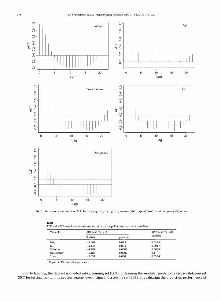
To examine the temporal structure of the available time series, the autocorrelation functions (ACF) are plotted in Fig. 3.The examination of the ACF of a series helps to uncover the stationary characteristics of the series and the degree of persis-tence in the data; a stationary and invertible time series have autocorrelations that exhibit fast exponential decay and henceshort-term memory, whereas the ACF of a series that exhibit long memory decay to a slow hyperbolic rate, reflecting dynam-ics where external shocks have a longer impact to the evolution of the phenomenon under examination (Karlaftis and Vlah-ogianni, 2009). McLeod and Hipel (1978) defined a long memory process as the one that has a non-finite quantity of theform: lim

n!1

Pnj¼�njqjj, where qj is the autocorrelation function at lag j of a discrete time series yt.

In the specific application, the decay in the ACF of both pollutants and traffic variables cannot be considered either hyper-bolic or exponential by a simple visual observation (Fig. 3). This, in relation to the irregular behavior observed in Figs. 1 and2, may imply the existence of non-stationarity in both pollutants and traffic time series, a situation not consistent with mostautoregressive time series models, e.g. the ARIMA models commonly used in modeling traffic and pollutants time series(Washington et al., 2010).

3.2. Testing against stationarity

A common approach in dealing with irregular time series is, first, to assume non-stationarity and, then, to difference thetime series d = 1, 2, . . . times to achieve covariance stationarity. In most transportation application parameter d is usually setto 1 (the series is then said to be integrated I(1)) and following, a Box–Jenkins approach (Box and Jenkins, 1970) is under-taken to model the series. However, this approach may lead to over-differentiation of the series and, consequently, an erro-neous correlation structure, in case the series is neither a I(0) or I(1) process and d should take values between �1 and 1(Granger and Joyeux, 1980).

We apply two tests to examine whether the available pollutants and traffic series are stationary, I(1) processes, or neitherof the above. The first test is the popular Augmented Dickey–Fuller (ADF) (MacKinnon, 1996), with the null hypothesis H0

that the series contain a unit root or should be I(1) integrated to achieve covariance stationarity and the KPSS (Kwiatkowski,Phillips, Schmidt, and Shin) test (Kwiatkowski et al., 1992) that evaluates the null hypothesis of a stationary I(0) process.

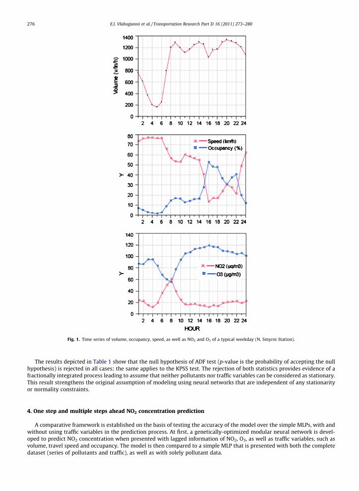
Fig. 1. Time series of volume, occupancy, speed, as well as NO2 and O3 of a typical weekday (N. Smyrni Station).

276 E.I. Vlahogianni et al. / Transportation Research Part D 16 (2011) 273–280

The results depicted in Table 1 show that the null hypothesis of ADF test (p-value is the probability of accepting the nullhypothesis) is rejected in all cases; the same applies to the KPSS test. The rejection of both statistics provides evidence of afractionally integrated process leading to assume that neither pollutants nor traffic variables can be considered as stationary.This result strengthens the original assumption of modeling using neural networks that are independent of any stationarityor normality constraints.

4. One step and multiple steps ahead NO2 concentration prediction

A comparative framework is established on the basis of testing the accuracy of the model over the simple MLPs, with andwithout using traffic variables in the prediction process. At first, a genetically-optimized modular neural network is devel-oped to predict NO2 concentration when presented with lagged information of NO2, O3, as well as traffic variables, such asvolume, travel speed and occupancy. The model is then compared to a simple MLP that is presented with both the completedataset (series of pollutants and traffic), as well as with solely pollutant data.

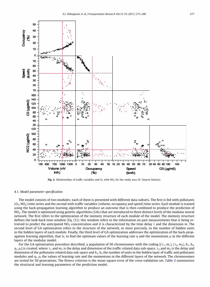
Fig. 2. Relationships of traffic variables and O3 with NO2 for the study area (N. Smyrni Station).

E.I. Vlahogianni et al. / Transportation Research Part D 16 (2011) 273–280 277

4.1. Model parameter specification

The model consists of two modules; each of them is presented with different data subsets. The first is fed with pollutants(O3, NO2) time series and the second with traffic variables (volume, occupancy and speed) time series. Each module is trainedusing the back-propagation learning algorithm to produce an outcome that is then combined to produce the prediction ofNO2. The model is optimized using genetic algorithms (GAs) that are introduced to three distinct levels of the modular neuralnetwork. The first refers to the optimization of the memory structure of each module of the model. The memory structuredefines the look-back time window (Eq. (5)); this window refers to the information on past measurements that is being re-trieved to predict the anticipated NO2 concentration and it is characterized by the time delay s and the dimension m. Thesecond level of GA optimization refers to the structure of the network, or more precisely, to the number of hidden unitsin the hidden layers of each module. Finally, the third level of GA optimization addresses the optimization of the back-prop-agation learning algorithm, that is, to find the optimum values of the learning rate g and the momentum l in the differentlayers of the modular model.

For the GA optimization procedure described, a population of 50 chromosomes with the coding {(s1, m1), (s2, m2), h1, h2,gi, li} is created, where s1 and m1 is the delay and dimension of the traffic-related data sub-space, s2 and m2 is the delay anddimension of the pollutants-related data sub-space and h1, h2 the number of units in the hidden layer of traffic and pollutantsmodules and gi, li the values of learning rate and the momentum in the different layers of the network. The chromosomesare tested for 50 generations. The fitness criterion is the mean square error of the cross-validation set. Table 2 summarizesthe structural and learning parameters of the prediction model.

0 5 10 15 20Lag

ACF

Lag

ACF

15 20

0 5 10 15 20Lag

ACF

Lag

ACF

0 5 10 15 20

0 5 10 15 20Lag

-0.4-0.2-0.0

0.20.40.60.81.0

0 5 10

0.0

0.2

0.4

0.6

0.8

1.0

-0.2

-0.0

0.2

0.4

0.6

1.0

-0.2

0.0

0.2

0.4

0.6

0.8

1.0

-0.2

-0.0

0.2

0.4

0.6

0.8

1.0

ACF

NO2

O3

Volume

Travel Speed

Occupancy

0.8

Fig. 3. Autocorrelation function (ACF) for NO2 (lg/m3), O3 (lg/m3), volume (vh/h), speed (km/h) and occupancy (%) series.

Table 1ADF and KPSS tests for unit root and stationarity for pollutants and traffic variables.

Variable ADF test H0: I(1) KPSS test H0: I(0)Statistic

Statistic p-Value

NO2 �3.061 0.013 0.0385*

O3 �4.134 0.003 0.0917*

Volume �4.497 0.0002 0.0695*

Occupancy �5.184 0.0002 0.11*

Speed �3.631 0.006 0.0364*

* Reject at 1% level of significance.

278 E.I. Vlahogianni et al. / Transportation Research Part D 16 (2011) 273–280

Prior to training, the dataset is divided into a training set (60%) for training the modular predictor, a cross-validation set(20%) for testing the training process against over-fitting and a testing set (20%) for evaluating the prediction performance of

Table 2Structural, learning and optimization specifications of the modular neural network.

Parameter Description Value

Input space Lagged information on traffic volume (vh/ln/h),occupancy (%), travel speed (km/h), O3 (lg/m3) and NO2

(lg/m3)Output space NO2 (lg/m3)Architecture Module Temporal NN

Memory (s, m) GA optimizedHidden layer GA optimizedActivation tan hOutput space 1

Learning rule Back-propagationGenetic algorithm Population 50

Generation 50Selection TournamentCrossover probability (pc) Uniform: 0.9Mutation probability (pm) 0.02Fitness function Mean square error

(cross-validation set)

Table 3Comparison of modeling approaches for 1 h ahead prediction.

Methodology Prediction step Input space Look-back time window Mean relative error (%)

Genetically-optimized modular MLP 1 Traffic/pollutants s = 1, m = 3 (traffic) 16.96s = 1, m = 4 (pollutants)

6 s = 1, m = 4 (traffic) 23.48s = 1, m = 8 (pollutants)

1 Only pollutants s = 1, m = 8 17.71

Genetically-optimized MLP 1 Traffic/pollutants s = 1, m = 3 (traffic) 24.63s = 1, m = 4 (pollutants)

1 Only pollutants s = 1, m = 8 24.19

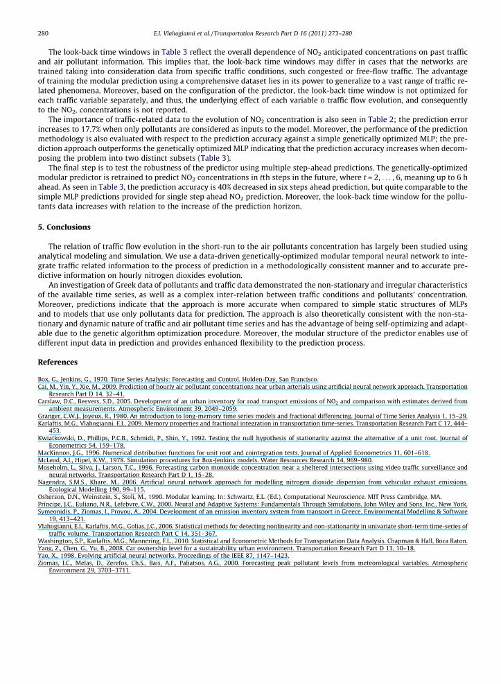
Fig. 4. Actual versus predicted values of NO2 using the modular genetically optimized prediction model.

E.I. Vlahogianni et al. / Transportation Research Part D 16 (2011) 273–280 279

the modular predictor. As the neural network operates under time series logic, database separation is based on entire dayconsideration to preserve data continuity in each subset.

The results of the NO2 prediction using the modular approach are illustrated in Table 3. The model can predict hourly NO2

concentration with 17.0% mean relative percent error using both traffic and pollutants data. As seen in Fig. 4 the predictionapproach provides a good approximation of the evolution of the actual NO2 values. The model seems to overestimate the lowvalues and underestimate larger ones. Regarding the look-back time window of prediction, Table 3 summarizes the inputspace for both traffic and pollutants-related data, as resulted from the genetic optimization. As can be observed, extendedinformation on the past evolution of pollutants is required when compared to traffic related information. More accurately,the optimized model ‘‘looks’’ four steps in the past for pollutants’ data and three steps in the past for traffic-related data topredict NO2 concentration one step ahead in the future.

280 E.I. Vlahogianni et al. / Transportation Research Part D 16 (2011) 273–280

The look-back time windows in Table 3 reflect the overall dependence of NO2 anticipated concentrations on past trafficand air pollutant information. This implies that, the look-back time windows may differ in cases that the networks aretrained taking into consideration data from specific traffic conditions, such congested or free-flow traffic. The advantageof training the modular prediction using a comprehensive dataset lies in its power to generalize to a vast range of traffic re-lated phenomena. Moreover, based on the configuration of the predictor, the look-back time window is not optimized foreach traffic variable separately, and thus, the underlying effect of each variable o traffic flow evolution, and consequentlyto the NO2, concentrations is not reported.

The importance of traffic-related data to the evolution of NO2 concentration is also seen in Table 2; the prediction errorincreases to 17.7% when only pollutants are considered as inputs to the model. Moreover, the performance of the predictionmethodology is also evaluated with respect to the prediction accuracy against a simple genetically optimized MLP; the pre-diction approach outperforms the genetically optimized MLP indicating that the prediction accuracy increases when decom-posing the problem into two distinct subsets (Table 3).

The final step is to test the robustness of the predictor using multiple step-ahead predictions. The genetically-optimizedmodular predictor is retrained to predict NO2 concentrations in tth steps in the future, where t = 2, . . . , 6, meaning up to 6 hahead. As seen in Table 3, the prediction accuracy is 40% decreased in six steps ahead prediction, but quite comparable to thesimple MLP predictions provided for single step ahead NO2 prediction. Moreover, the look-back time window for the pollu-tants data increases with relation to the increase of the prediction horizon.

5. Conclusions

The relation of traffic flow evolution in the short-run to the air pollutants concentration has largely been studied usinganalytical modeling and simulation. We use a data-driven genetically-optimized modular temporal neural network to inte-grate traffic related information to the process of prediction in a methodologically consistent manner and to accurate pre-dictive information on hourly nitrogen dioxides evolution.

An investigation of Greek data of pollutants and traffic data demonstrated the non-stationary and irregular characteristicsof the available time series, as well as a complex inter-relation between traffic conditions and pollutants’ concentration.Moreover, predictions indicate that the approach is more accurate when compared to simple static structures of MLPsand to models that use only pollutants data for prediction. The approach is also theoretically consistent with the non-sta-tionary and dynamic nature of traffic and air pollutant time series and has the advantage of being self-optimizing and adapt-able due to the genetic algorithm optimization procedure. Moreover, the modular structure of the predictor enables use ofdifferent input data in prediction and provides enhanced flexibility to the prediction process.

References

Box, G., Jenkins, G., 1970. Time Series Analysis: Forecasting and Control. Holden-Day, San Francisco.Cai, M., Yin, Y., Xie, M., 2009. Prediction of hourly air pollutant concentrations near urban arterials using artificial neural network approach. Transportation

Research Part D 14, 32–41.Carslaw, D.C., Beevers, S.D., 2005. Development of an urban inventory for road transport emissions of NO2 and comparison with estimates derived from

ambient measurements. Atmospheric Environment 39, 2049–2059.Granger, C.W.J., Joyeux, R., 1980. An introduction to long-memory time series models and fractional differencing. Journal of Time Series Analysis 1, 15–29.Karlaftis, M.G., Vlahogianni, E.I., 2009. Memory properties and fractional integration in transportation time-series. Transportation Research Part C 17, 444–

453.Kwiatkowski, D., Phillips, P.C.B., Schmidt, P., Shin, Y., 1992. Testing the null hypothesis of stationarity against the alternative of a unit root. Journal of

Econometrics 54, 159–178.MacKinnon, J.G., 1996. Numerical distribution functions for unit root and cointegration tests. Journal of Applied Econometrics 11, 601–618.McLeod, A.I., Hipel, K.W., 1978. Simulation procedures for Box-Jenkins models. Water Resources Research 14, 969–980.Moseholm, L., Silva, J., Larson, T.C., 1996. Forecasting carbon monoxide concentration near a sheltered intersections using video traffic surveillance and

neural networks. Transportation Research Part D 1, 15–28.Nagendra, S.M.S., Khare, M., 2006. Artificial neural network approach for modelling nitrogen dioxide dispersion from vehicular exhaust emissions.

Ecological Modelling 190, 99–115.Osherson, D.N., Weinstein, S., Stoli, M., 1990. Modular learning. In: Schwartz, E.L. (Ed.), Computational Neuroscience. MIT Press Cambridge, MA.Príncipe, J.C., Euliano, N.R., Lefebvre, C.W., 2000. Neural and Adaptive Systems: Fundamentals Through Simulations. John Wiley and Sons, Inc., New York.Symeonidis, P., Ziomas, I., Proyou, A., 2004. Development of an emission inventory system from transport in Greece. Environmental Modelling & Software

19, 413–421.Vlahogianni, E.I., Karlaftis, M.G., Golias, J.C., 2006. Statistical methods for detecting nonlinearity and non-stationarity in univariate short-term time-series of

traffic volume. Transportation Research Part C 14, 351–367.Washington, S.P., Karlaftis, M.G., Mannering, F.L., 2010. Statistical and Econometric Methods for Transportation Data Analysis. Chapman & Hall, Boca Raton.Yang, Z., Chen, G., Yu, B., 2008. Car ownership level for a sustainability urban environment. Transportation Research Part D 13, 10–18.Yao, X., 1998. Evolving artificial neural networks. Proceedings of the IEEE 87, 1147–1423.Ziomas, I.C., Melas, D., Zerefos, Ch.S., Bais, A.F., Paliatsos, A.G., 2000. Forecasting peak pollutant levels from meteorological variables. Atmospheric

Environment 29, 3703–3711.