long-range time-correlation properties of seismic sequences
TRANSCRIPT
Chaos, Solitons and Fractals 21 (2004) 387–393
www.elsevier.com/locate/chaos
Long-range time-correlation properties of seismic sequences
Luciano Telesca a,*, Vincenzo Lapenna a, Michele Lovallo a, Maria Macchiato b
a Institute of Methodologies for Environmental Analysis, National Research Council, IMAA-CNR, C. da S. Loja,
I-85050 Tito Scalo (PZ), Italyb Dipartimento di Scienze Fisiche, Universit�a ‘‘Federico II’’, Naples 80125, Italy
Accepted 10 December 2003
Communicated by I. Antoniou
Abstract
We performed the Allan factor analysis on the temporal distribution of seismicity of Italy from 1983 to 2002.
Significant power-law temporal behaviour has been identified analyzing both the full and the aftershock-depleted
seismic catalogues of Italy; this suggests that the correlated behaviour is due not only to the generation of aftershocks,
following the occurrence of large shocks, but is a feature of the background seismicity.
� 2004 Elsevier Ltd. All rights reserved.
1. Introduction
Earthquakes are a complex phenomenon in space and time domains. The distribution of the magnitudes of the
earthquakes follows the Gutenberg–Richter [1] power-law. The epicenter distribution is fractal in space and also the
faults have a fractal-like structure [2]. The Omori’s law establishes the presence of short-range temporal correlation
between earthquakes, stating that after a main large shock a series of aftershocks occurs, with a power-law time-fre-
quency decay [3].
Therefore, tectonic processes are considered to display fractal properties in time (e.g. [4–6]). Identifying whether the
time-occurrences of earthquakes are independent on each other or not, leads to the assessment of the statistical dis-
tribution ruling the event occurrence. Several distributions have been used to model seismic activity. Poisson statistics
has been undoubtly the most extensively used, since, in many cases, for large events a simple discrete Poisson distri-
bution provides a close fit [7]. But the complexity of the earthquake dynamics has revealed the presence of time-
clustering at both short and long timescales [2]. The analysis of the temporal variations of the scaling properties of
earthquakes has been used to characterize the main features of seismicity and to bring us insight the inner dynamics of
seismotectonic activity. The evolution of scaling exponents with respect to time has revealed the increase of the time-
clustering feature of seismicity corresponding to large events, mostly due to the aftershock activation [8]. The depth-
dependent variation of the time-clustering behaviour of seismicity has been interpreted in relation with the brittle and
ductile behaviour of the crust vs. depth [9].
The objective of this study is to analyze the spatial distribution of the long-range time correlation properties of the
Italian seismicity, investigated using the Allan factor analysis (AFA).
* Corresponding author. Tel.: +39-0971-427206; fax: +39-0971-427271.
E-mail address: [email protected] (L. Telesca).
0960-0779/$ - see front matter � 2004 Elsevier Ltd. All rights reserved.
doi:10.1016/j.chaos.2003.12.009
388 L. Telesca et al. / Chaos, Solitons and Fractals 21 (2004) 387–393
2. Methods
The standard technique to investigate the temporal properties of a time series is the power spectral density (PSD)
Sðf Þ, obtained by means of a Fourier transform of the signal. The PSD informs on how the power is concentrated at
various frequency bands. This information allows one to identify periodic, multi-periodic or non-periodic behaviours.
Usually the logarithmic power spectrum plot is used to better distinguish between the broadband and periodic com-
ponents. The power-law dependence (linear on a log–log plot) of the PSD, given by Sðf Þ � f a, is a hallmark of the
presence of long-range correlated properties in the data. The properties of the signal can be further classified in terms of
the numerical value of the spectral exponent a: if a ¼ 0, the signal is a realization of a white noise process, and is not
characterized by any kind of time correlation; if a > 0, the signal possesses the tendency for repeating the sign of its
fluctuations (i.e. if it increases in one period it will very likely increase in the next period), and, thus, it is persistent; if
a < 0, the signal is antipersistent and the fluctuations of opposite signs tend to alternate [10].
But, how to estimate a for a seismic sequence, for which it is not possible to simply calculate its Fourier Transform,
and then the PSD? This question is crucial, since our aim is to investigate the properties of the temporal fluctuations of
the seismicity.
The estimation of a or other parameter related to it, can be performed as follows. The approach consists into
representing a seismic sequence as a temporal point process, which describes events that occur at some random
locations in time [11], and expressed by a finite sum of Dirac’s delta functions centered on the occurrence times ti, withamplitude Ai proportional to the magnitude of the earthquake:
yðtÞ ¼XNi¼1
Aidðt � tiÞ; ð1Þ
where N represents the number of events recorded. In this representation we assume that there is an objective ‘‘clock’’
for the timing of the event.
Let us divide the time axis into equally spaced contiguous counting windows of duration s, and produce a sequence
of counts fZkðsÞg, with ZkðsÞ denoting the number of earthquakes in the kth window:
Zkðs; tÞ ¼Z tk
tk�1
Xn
j¼1
dðt � tjÞdt: ð2Þ
The Allan factor analysis (AFA) concerns the calculation of the Allan factor (AF), that is a measure which can be
used to distinguish fractal from Poissonian temporal fluctuations in point processes. This factor is defined as the
variance of successive counts for a specified counting time s divided by twice the mean number of events in that
counting time:
AFðsÞ ¼ hðZkþ1ðsÞ � ZkðsÞÞ2i2hZkðsÞi
: ð3Þ
The AF of a fractal point process varies with the counting time s with a power-law form:
AFðsÞ ¼ 1þ ss1
� �a
: ð4Þ
The monotonic power-law increase is representative of the presence of fluctuations on many time scales [12]; s1 is theso-called fractal onset time, and marks the lower limit for significant scaling behaviour in the AF, so that for s � s1 theclustering property becomes negligible within these timescales [13]. For Poissonian processes the AF assumes
approximately values near or below unity for all counting times s. From Eq. (4), the calculation of a can be performed
by estimating the slope of the straight line that fits in a least square sense the AF curve, plotted in log–log scales. Of
course, only the linear part of the curve will be considered to calculate the fractal exponent.
3. Data analysis
We have investigated the shallow (depth 6 100 km) Italian seismicity from 1983 to 2002, considering the earth-
quakes contained in a polygonal area surrounding the Italian coasts and borders within which the National Institute of
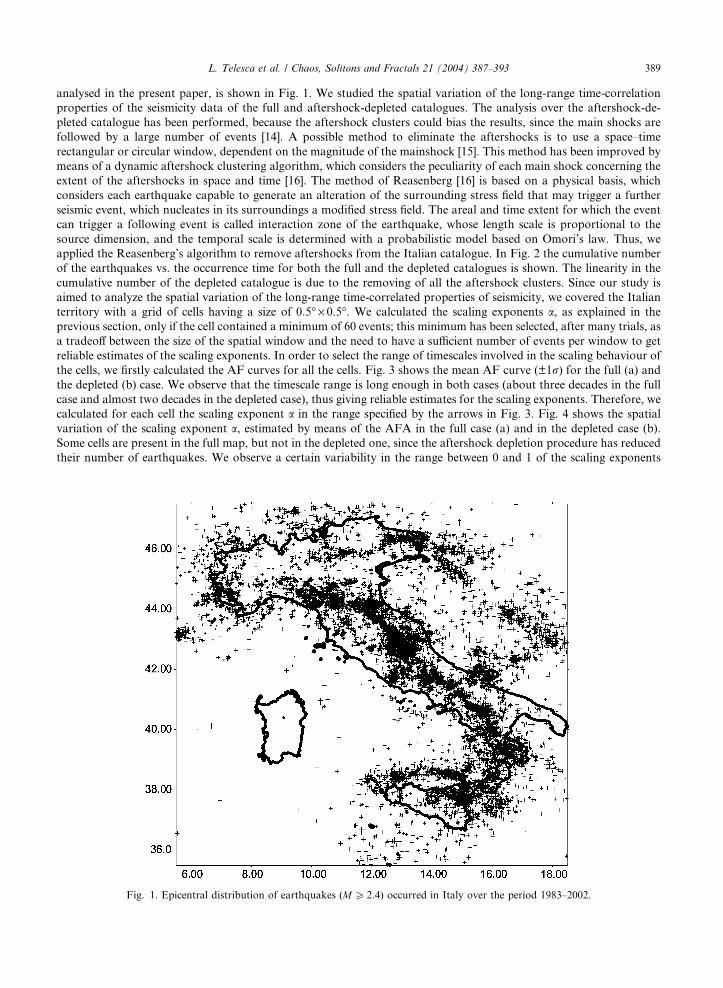
Geophysics and Volcanology has furnished reliable locations for the events of magnitude M P 2:4, that represents theminimum magnitude for which the catalogue can be considered complete. The spatial distribution of the earthquakes,
L. Telesca et al. / Chaos, Solitons and Fractals 21 (2004) 387–393 389
analysed in the present paper, is shown in Fig. 1. We studied the spatial variation of the long-range time-correlation
properties of the seismicity data of the full and aftershock-depleted catalogues. The analysis over the aftershock-de-
pleted catalogue has been performed, because the aftershock clusters could bias the results, since the main shocks are
followed by a large number of events [14]. A possible method to eliminate the aftershocks is to use a space–time
rectangular or circular window, dependent on the magnitude of the mainshock [15]. This method has been improved by
means of a dynamic aftershock clustering algorithm, which considers the peculiarity of each main shock concerning the
extent of the aftershocks in space and time [16]. The method of Reasenberg [16] is based on a physical basis, which
considers each earthquake capable to generate an alteration of the surrounding stress field that may trigger a further
seismic event, which nucleates in its surroundings a modified stress field. The areal and time extent for which the event
can trigger a following event is called interaction zone of the earthquake, whose length scale is proportional to the
source dimension, and the temporal scale is determined with a probabilistic model based on Omori’s law. Thus, we
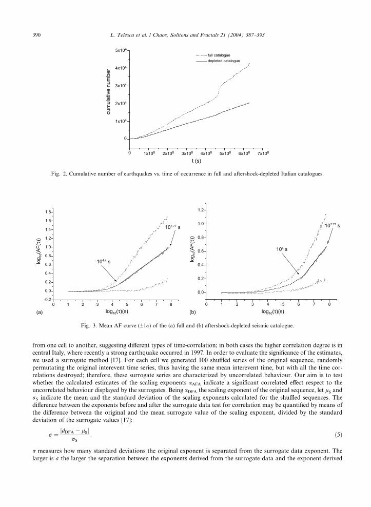
applied the Reasenberg’s algorithm to remove aftershocks from the Italian catalogue. In Fig. 2 the cumulative number
of the earthquakes vs. the occurrence time for both the full and the depleted catalogues is shown. The linearity in the
cumulative number of the depleted catalogue is due to the removing of all the aftershock clusters. Since our study is
aimed to analyze the spatial variation of the long-range time-correlated properties of seismicity, we covered the Italian
territory with a grid of cells having a size of 0.5� · 0.5�. We calculated the scaling exponents a, as explained in the
previous section, only if the cell contained a minimum of 60 events; this minimum has been selected, after many trials, as
a tradeoff between the size of the spatial window and the need to have a sufficient number of events per window to get
reliable estimates of the scaling exponents. In order to select the range of timescales involved in the scaling behaviour of
the cells, we firstly calculated the AF curves for all the cells. Fig. 3 shows the mean AF curve (±1r) for the full (a) andthe depleted (b) case. We observe that the timescale range is long enough in both cases (about three decades in the full
case and almost two decades in the depleted case), thus giving reliable estimates for the scaling exponents. Therefore, we
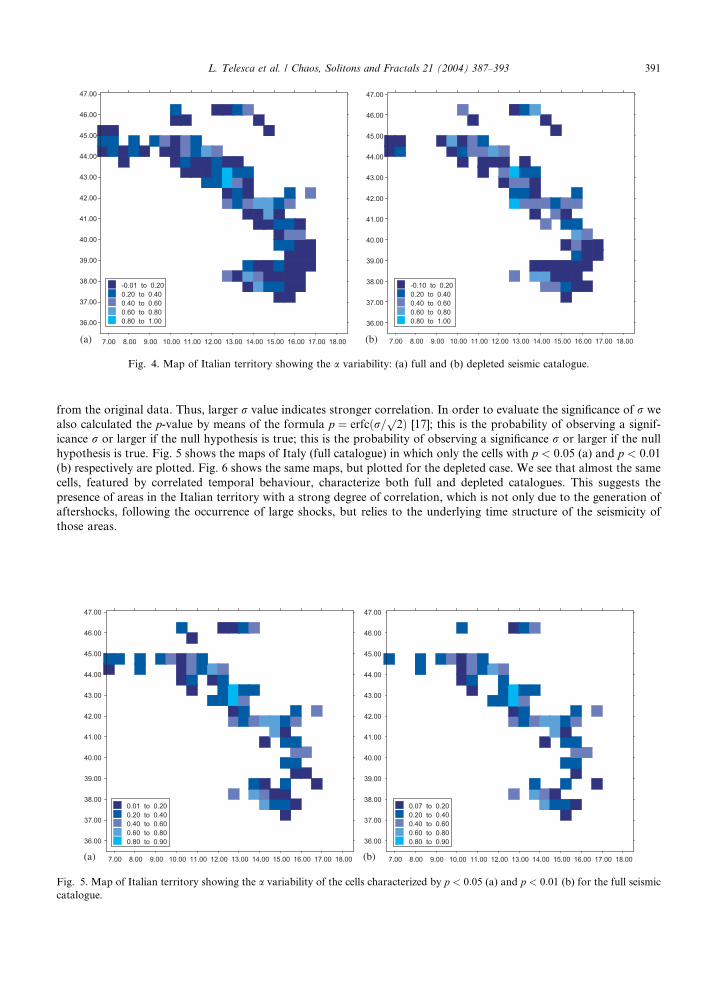
calculated for each cell the scaling exponent a in the range specified by the arrows in Fig. 3. Fig. 4 shows the spatial
variation of the scaling exponent a, estimated by means of the AFA in the full case (a) and in the depleted case (b).
Some cells are present in the full map, but not in the depleted one, since the aftershock depletion procedure has reduced
their number of earthquakes. We observe a certain variability in the range between 0 and 1 of the scaling exponents
Fig. 1. Epicentral distribution of earthquakes (M P 2:4) occurred in Italy over the period 1983–2002.
0 1 2 3 4 5 6 7 8-0.2
0.0
0.2
0.4
0.6
0.8
1.0
1.2
1.4
1.6
1.8
107.77 s
104.4 s
107.77 s
106 s
log 1
0(AF(
τ))
log10(τ)(s)0 1 2 3 4 5 6 7 8
0.0
0.2
0.4
0.6
0.8
1.0
1.2
log 1
0(AF(
τ))
log10(τ)(s)(a) (b)
Fig. 3. Mean AF curve (±1r) of the (a) full and (b) aftershock-depleted seismic catalogue.
0 1x10⁸ 2x10⁸ 3x10⁸ 4x10⁸ 5x10⁸ 6x10⁸ 7x10⁸
0
1x10⁴
2x10⁴
3x10⁴
4x10⁴
5x10⁴
full catalogue depleted catalogue
cum
ulat
ive
num
ber
t (s)
Fig. 2. Cumulative number of earthquakes vs. time of occurrence in full and aftershock-depleted Italian catalogues.
390 L. Telesca et al. / Chaos, Solitons and Fractals 21 (2004) 387–393
from one cell to another, suggesting different types of time-correlation; in both cases the higher correlation degree is in
central Italy, where recently a strong earthquake occurred in 1997. In order to evaluate the significance of the estimates,
we used a surrogate method [17]. For each cell we generated 100 shuffled series of the original sequence, randomly
permutating the original interevent time series, thus having the same mean interevent time, but with all the time cor-
relations destroyed; therefore, these surrogate series are characterized by uncorrelated behaviour. Our aim is to test
whether the calculated estimates of the scaling exponents aAFA indicate a significant correlated effect respect to the
uncorrelated behaviour displayed by the surrogates. Being aDFA the scaling exponent of the original sequence, let lS and
rS indicate the mean and the standard deviation of the scaling exponents calculated for the shuffled sequences. The
difference between the exponents before and after the surrogate data test for correlation may be quantified by means of
the difference between the original and the mean surrogate value of the scaling exponent, divided by the standard
deviation of the surrogate values [17]:
r ¼ jdDFA � lSjrS
: ð5Þ
r measures how many standard deviations the original exponent is separated from the surrogate data exponent. The
larger is r the larger the separation between the exponents derived from the surrogate data and the exponent derived
7.00 8.00 9.00 10.00 11.00 12.00 13.00 14.00 15.00 16.00 17.00 18.00
36.00
37.00
38.00
39.00
40.00
41.00
42.00
43.00
44.00
45.00
46.00
47.00
-0.01 to 0.20 0.20 to 0.40 0.40 to 0.60 0.60 to 0.80 0.80 to 1.00
7.00 8.00 9.00 10.00 11.00 12.00 13.00 14.00 15.00 16.00 17.00 18.00
36.00
37.00
38.00
39.00
40.00
41.00
42.00
43.00
44.00
45.00
46.00
47.00
-0.10 to 0.20 0.20 to 0.40 0.40 to 0.60 0.60 to 0.80 0.80 to 1.00
(a) (b)
Fig. 4. Map of Italian territory showing the a variability: (a) full and (b) depleted seismic catalogue.
L. Telesca et al. / Chaos, Solitons and Fractals 21 (2004) 387–393 391
from the original data. Thus, larger r value indicates stronger correlation. In order to evaluate the significance of r we
also calculated the p-value by means of the formula p ¼ erfcðr=p2Þ [17]; this is the probability of observing a signif-
icance r or larger if the null hypothesis is true; this is the probability of observing a significance r or larger if the null
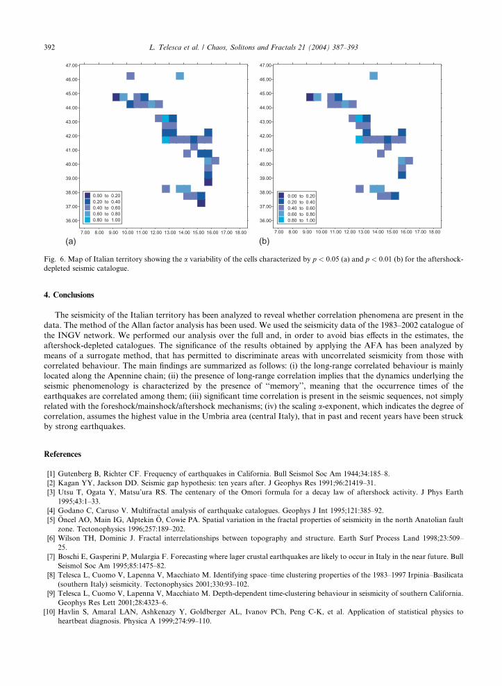
hypothesis is true. Fig. 5 shows the maps of Italy (full catalogue) in which only the cells with p < 0:05 (a) and p < 0:01(b) respectively are plotted. Fig. 6 shows the same maps, but plotted for the depleted case. We see that almost the same
cells, featured by correlated temporal behaviour, characterize both full and depleted catalogues. This suggests the
presence of areas in the Italian territory with a strong degree of correlation, which is not only due to the generation of
aftershocks, following the occurrence of large shocks, but relies to the underlying time structure of the seismicity of
those areas.
7.00 8.00 9.00 10.00 11.00 12.00 13.00 14.00 15.00 16.00 17.00 18.00
36.00
37.00
38.00
39.00
40.00
41.00
42.00
43.00
44.00
45.00
46.00
47.00
0.01 to 0.20 0.20 to 0.40 0.40 to 0.60 0.60 to 0.80 0.80 to 0.90
7.00 8.00 9.00 10.00 11.00 12.00 13.00 14.00 15.00 16.00 17.00 18.00
36.00
37.00
38.00
39.00
40.00
41.00
42.00
43.00
44.00
45.00
46.00
47.00
0.07 to 0.20 0.20 to 0.40 0.40 to 0.60 0.60 to 0.80 0.80 to 0.90
(a) (b)
Fig. 5. Map of Italian territory showing the a variability of the cells characterized by p < 0:05 (a) and p < 0:01 (b) for the full seismic
catalogue.
7.00 8.00 9.00 10.00 11.00 12.00 13.00 14.00 15.00 16.00 17.00 18.00
36.00
37.00
38.00
39.00
40.00
41.00
42.00
43.00
44.00
45.00
46.00
47.00
7.00 8.00 9.00 10.00 11.00 12.00 13.00 14.00 15.00 16.00 17.00 18.00
36.00
37.00
38.00
39.00
40.00
41.00
42.00
43.00
44.00
45.00
46.00
47.00
0.00 to 0.20 0.20 to 0.40 0.40 to 0.60 0.60 to 0.80 0.80 to 1.00
0.00 to 0.20 0.20 to 0.40 0.40 to 0.60 0.60 to 0.80 0.80 to 1.00
(a) (b)
Fig. 6. Map of Italian territory showing the a variability of the cells characterized by p < 0:05 (a) and p < 0:01 (b) for the aftershock-
depleted seismic catalogue.
392 L. Telesca et al. / Chaos, Solitons and Fractals 21 (2004) 387–393
4. Conclusions
The seismicity of the Italian territory has been analyzed to reveal whether correlation phenomena are present in the
data. The method of the Allan factor analysis has been used. We used the seismicity data of the 1983–2002 catalogue of
the INGV network. We performed our analysis over the full and, in order to avoid bias effects in the estimates, the
aftershock-depleted catalogues. The significance of the results obtained by applying the AFA has been analyzed by
means of a surrogate method, that has permitted to discriminate areas with uncorrelated seismicity from those with
correlated behaviour. The main findings are summarized as follows: (i) the long-range correlated behaviour is mainly
located along the Apennine chain; (ii) the presence of long-range correlation implies that the dynamics underlying the
seismic phenomenology is characterized by the presence of ‘‘memory’’, meaning that the occurrence times of the
earthquakes are correlated among them; (iii) significant time correlation is present in the seismic sequences, not simply
related with the foreshock/mainshock/aftershock mechanisms; (iv) the scaling a-exponent, which indicates the degree of
correlation, assumes the highest value in the Umbria area (central Italy), that in past and recent years have been struck
by strong earthquakes.
References
[1] Gutenberg B, Richter CF. Frequency of earthquakes in California. Bull Seismol Soc Am 1944;34:185–8.
[2] Kagan YY, Jackson DD. Seismic gap hypothesis: ten years after. J Geophys Res 1991;96:21419–31.
[3] Utsu T, Ogata Y, Matsu’ura RS. The centenary of the Omori formula for a decay law of aftershock activity. J Phys Earth
1995;43:1–33.
[4] Godano C, Caruso V. Multifractal analysis of earthquake catalogues. Geophys J Int 1995;121:385–92.
[5] €Oncel AO, Main IG, Alptekin €O, Cowie PA. Spatial variation in the fractal properties of seismicity in the north Anatolian fault
zone. Tectonophysics 1996;257:189–202.
[6] Wilson TH, Dominic J. Fractal interrelationships between topography and structure. Earth Surf Process Land 1998;23:509–
25.
[7] Boschi E, Gasperini P, Mulargia F. Forecasting where lager crustal earthquakes are likely to occur in Italy in the near future. Bull
Seismol Soc Am 1995;85:1475–82.
[8] Telesca L, Cuomo V, Lapenna V, Macchiato M. Identifying space–time clustering properties of the 1983–1997 Irpinia–Basilicata
(southern Italy) seismicity. Tectonophysics 2001;330:93–102.
[9] Telesca L, Cuomo V, Lapenna V, Macchiato M. Depth-dependent time-clustering behaviour in seismicity of southern California.
Geophys Res Lett 2001;28:4323–6.
[10] Havlin S, Amaral LAN, Ashkenazy Y, Goldberger AL, Ivanov PCh, Peng C-K, et al. Application of statistical physics to
heartbeat diagnosis. Physica A 1999;274:99–110.
L. Telesca et al. / Chaos, Solitons and Fractals 21 (2004) 387–393 393
[11] Cox DR, Isham V. Point processes. London: Chapman and Hall; 1980.
[12] Lowen SB, Teich MC. Estimation and simulation of fractal stochastic point processes. Fractals 1995;3:183–210.
[13] Thurner S, Lowen SB, Feurstein MC, Heneghan C, Feichtinger HG, Teich MC. Analysis, synthesis, and estimation of fractal-rate
stochastic point processes. Fractals 1997;5:565–96.
[14] Breitenberg C. Non-random spectral components in the seismicity of NE Italy. Earth Planet Sci Lett 2000;179:379–90.
[15] Gardner JK, Knopoff L. Statistical search for non-random features of the seismicity of strong earthquakes. Phys Earth Planet Int
1976;12:291–318.
[16] Reasenberg P. Second-order moment of central California seismicity, 1969–1982. J Geophys Res 1985;90:5479–95.
[17] Theiler J, Eubank S, Longtin A, Galdrikian B, Farmer JD. Testing for nonlinearity in time series: the method of surrogate data.
Physica D 1992;58:77–94.