sequences and difference equations
TRANSCRIPT
ASequences and Difference Equations
From mathematics you probably know the concept of a sequence, which is nothingbut a collection of numbers with a specific order. A general sequence is written as
x0; x1; x2; : : : ; xn; : : : ;
One example is the sequence of all odd numbers:
1; 3; 5; 7; : : : ; 2n C 1; : : :
For this sequence we have an explicit formula for the n-th term: 2nC1, and n takeson the values 0, 1, 2, : : :. We can write this sequence more compactly as .xn/1
nD0
with xn D 2n C 1. Other examples of infinite sequences from mathematics are
1; 4; 9; 16; 25; : : : .xn/1nD0; xn D .n C 1/2; (A.1)
1;1
2;
1
3;
1
4; : : : .xn/1
nD0; xn D 1
n C 1: (A.2)
The former sequences are infinite, because they are generated from all integers� 0 and there are infinitely many such integers. Nevertheless, most sequences fromreal life applications are finite. If you put an amount x0 of money in a bank, youwill get an interest rate and therefore have an amount x1 after one year, x2 after twoyears, and xN after N years. This process results in a finite sequence of amounts
x0; x1; x2; : : : ; xN ; .xn/NnD0 :
Usually we are interested in quite small N values (typically N � 20�30). Anyway,the life of the bank is finite, so the sequence definitely has an end.
For some sequences it is not so easy to set up a general formula for the n-th term.Instead, it is easier to express a relation between two or more consecutive elements.One example where we can do both things is the sequence of odd numbers. Thissequence can alternatively be generated by the formula
xnC1 D xn C 2 : (A.3)
645© Springer-Verlag Berlin Heidelberg 2016H.P. Langtangen, A Primer on Scientific Programming with Python,Texts in Computational Science and Engineering 6, DOI 10.1007/978-3-662-49887-3
646 A Sequences and Difference Equations
To start the sequence, we need an initial condition where the value of the first ele-ment is specified:
x0 D 1 :
Relations like (A.3) between consecutive elements in a sequence is called recur-rence relations or difference equations. Solving a difference equation can be quitechallenging in mathematics, but it is almost trivial to solve it on a computer. Thatis why difference equations are so well suited for computer programming, and thepresent appendix is devoted to this topic. Necessary background knowledge is pro-gramming with loops, arrays, and command-line arguments and visualization ofa function of one variable.
The program examples regarding difference equations are found in the foldersrc/diffeq1.
A.1 Mathematical Models Based on Difference Equations
The objective of science is to understand complex phenomena. The phenomenonunder consideration may be a part of nature, a group of social individuals, the trafficsituation in Los Angeles, and so forth. The reason for addressing something in a sci-entific manner is that it appears to be complex and hard to comprehend. A commonscientific approach to gain understanding is to create a model of the phenomenon,and discuss the properties of the model instead of the phenomenon. The basic ideais that the model is easier to understand, but still complex enough to preserve thebasic features of the problem at hand.
Essentially, all models are wrong, but some are useful. George E. P. Box, statistician,1919–2013.
Modeling is, indeed, a general idea with applications far beyond science. Sup-pose, for instance, that you want to invite a friend to your home for the first time.To assist your friend, you may send a map of your neighborhood. Such a map isa model: it exposes the most important landmarks and leaves out billions of detailsthat your friend can do very well without. This is the essence of modeling: a goodmodel should be as simple as possible, but still rich enough to include the importantstructures you are looking for.
Everything should be made as simple as possible, but not simpler.Paraphrased quote attributed to Albert Einstein, physicist, 1879–1955.
Certainly, the tools we apply to model a certain phenomenon differ a lot in vari-ous scientific disciplines. In the natural sciences, mathematics has gained a uniqueposition as the key tool for formulating models. To establish a model, you needto understand the problem at hand and describe it with mathematics. Usually, thisprocess results in a set of equations, i.e., the model consists of equations that mustbe solved in order to see how realistically the model describes a phenomenon. Dif-ference equations represent one of the simplest yet most effective type of equations
1 http://tinyurl.com/pwyasaa/diffeq
A.1 Mathematical Models Based on Difference Equations 647
arising in mathematical models. The mathematics is simple and the programmingis simple, thereby allowing us to focus more on the modeling part. Below we willderive and solve difference equations for diverse applications.
A.1.1 Interest Rates
Our first difference equation model concerns how much money an initial amountx0 will grow to after n years in a bank with annual interest rate p. You learned inschool the formula
xn D x0
�1 C p
100
�n
: (A.4)
Unfortunately, this formula arises after some limiting assumptions, like that ofa constant interest rate over all the n years. Moreover, the formula only gives usthe amount after each year, not after some months or days. It is much easier tocompute with interest rates if we set up a more fundamental model in terms ofa difference equation and then solve this equation on a computer.
The fundamental model for interest rates is that an amount xn�1 at some point oftime tn�1 increases its value with p percent to an amount xn at a new point of timetn:
xn D xn�1 C p
100xn�1 : (A.5)
If n counts years, p is the annual interest rate, and if p is constant, we can withsome arithmetics derive the following solution to (A.5):
xn D�1 C p
100
�xn�1 D
�1 C p
100
�2
xn�2 D : : : D�1 C p
100
�n
x0 :
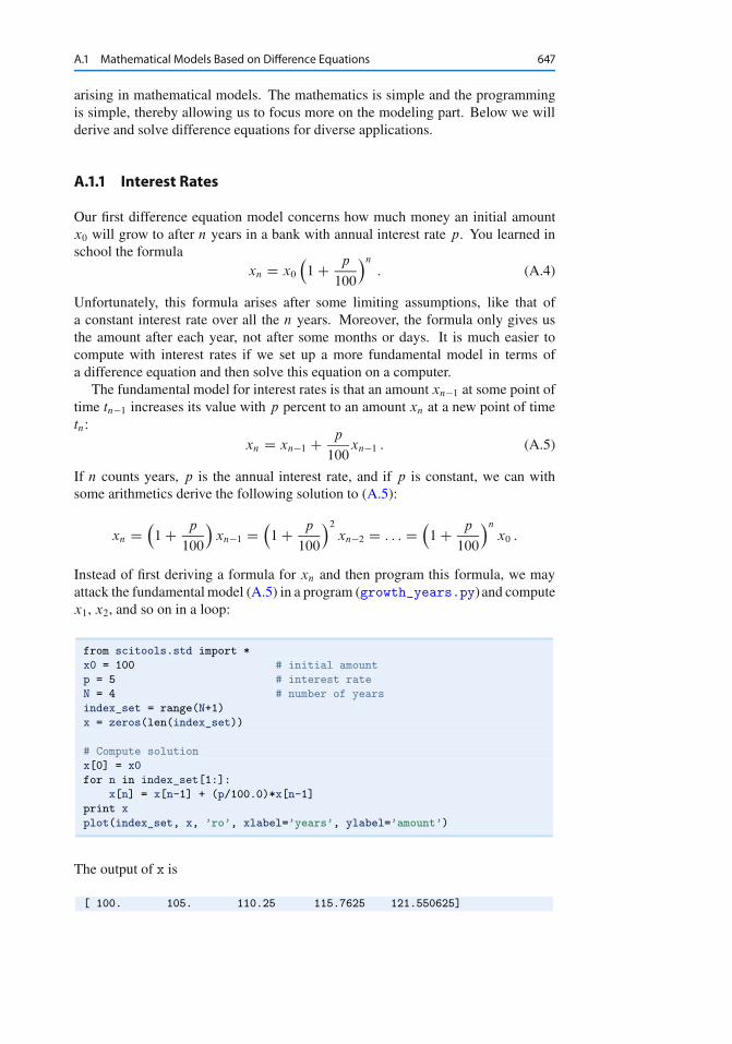
Instead of first deriving a formula for xn and then program this formula, we mayattack the fundamentalmodel (A.5) in a program (growth_years.py) and computex1, x2, and so on in a loop:
from scitools.std import *
x0 = 100 # initial amount
p = 5 # interest rate
N = 4 # number of years
index_set = range(N+1)
x = zeros(len(index_set))
# Compute solution
x[0] = x0
for n in index_set[1:]:
x[n] = x[n-1] + (p/100.0)*x[n-1]
print x
plot(index_set, x, ’ro’, xlabel=’years’, ylabel=’amount’)
The output of x is
[ 100. 105. 110.25 115.7625 121.550625]
648 A Sequences and Difference Equations
Programmers of mathematical software who are trained in making programs moreefficient, will notice that it is not necessary to store all the xn values in an array oruse a list with all the indices 0; 1; : : : ; N . Just one integer for the index and twofloats for xn and xn�1 are strictly necessary. This can save quite some memoryfor large values of N . Exercise A.3 asks you to develop such a memory-efficientprogram.
Suppose now that we are interested in computing the growth of money after N
days instead. The interest rate per day is taken as r D p=D if p is the annualinterest rate and D is the number of days in a year. The fundamental model is thesame, but now n counts days and p is replaced by r :
xn D xn�1 C r
100xn�1 : (A.6)
A common method in international business is to choose D D 360, yet let n countthe exact number of days between two dates (see the Wikipedia entry Day countconvention2 for an explanation). Python has a module datetime for convenientcalculations with dates and times. To find the number of days between two dates,we perform the following operations:
>>> import datetime
>>> date1 = datetime.date(2007, 8, 3) # Aug 3, 2007
>>> date2 = datetime.date(2008, 8, 4) # Aug 4, 2008
>>> diff = date2 - date1
>>> print diff.days
367
We can modify the previous program to compute with days instead of years:
from scitools.std import *
x0 = 100 # initial amount
p = 5 # annual interest rate
r = p/360.0 # daily interest rate
import datetime
date1 = datetime.date(2007, 8, 3)
date2 = datetime.date(2011, 8, 3)
diff = date2 - date1
N = diff.days
index_set = range(N+1)
x = zeros(len(index_set))
# Compute solution
x[0] = x0
for n in index_set[1:]:
x[n] = x[n-1] + (r/100.0)*x[n-1]
print x
plot(index_set, x, ’ro’, xlabel=’days’, ylabel=’amount’)
Running this program, called growth_days.py, prints out 122.5 as the finalamount.
2 http://en.wikipedia.org/wiki/Day_count_convention
A.1 Mathematical Models Based on Difference Equations 649
It is quite easy to adjust the formula (A.4) to the case where the interest is addedevery day instead of every year. However, the strength of the model (A.6) and theassociated program growth_days.py becomes apparent when r varies in time –and this is what happens in real life. In the model we can just write r.n/ to explic-itly indicate the dependence upon time. The corresponding time-dependent annualinterest rate is what is normally specified, and p.n/ is usually a piecewise constantfunction (the interest rate is changed at some specific dates and remains constantbetween these days). The construction of a corresponding array p in a program,given the dates when p changes, can be a bit tricky since we need to compute thenumber of days between the dates of changes and index p properly. We do notdive into these details now, but readers who want to compute p and who is readyfor some extra brain training and index puzzling can attack Exercise A.8. For nowwe assume that an array p holds the time-dependent annual interest rates for eachday in the total time period of interest. The growth_days.py program then needsa slight modification, typically,
p = zeros(len(index_set))
# set up p (might be challenging!)
r = p/360.0 # daily interest rate
...
for n in index_set[1:]:
x[n] = x[n-1] + (r[n-1]/100.0)*x[n-1]
For the very simple (and not-so-relevant) case where p grows linearly (i.e., dailychanges) from 4 to 6 percent over the period of interest, we have made a completeprogram in the file growth_days_timedep.py. You can compare a simulationwith linearly varying p between 4 and 6 and a simulation using the average p value5 throughout the whole time interval.
A difference equation with r.n/ is quite difficult to solve mathematically, but then-dependence in r is easy to deal with in the computerized solution approach.
A.1.2 The Factorial as a Difference Equation
The difference equationxn D nxn�1; x0 D 1 (A.7)
can quickly be solved recursively:
xn D nxn�1
D n.n � 1/xn�2
D n.n � 1/.n � 2/xn�3
D n.n � 1/.n � 2/ � � � 1 :
The result xn is nothing but the factorial of n, denoted as nŠ. Equation (A.7) thengives a standard recipe to compute nŠ.
650 A Sequences and Difference Equations
A.1.3 Fibonacci Numbers
Every textbook with somematerial on sequences usually presents a difference equa-tion for generating the famous Fibonacci numbers3:
xn D xn�1 C xn�2; x0 D 1; x1 D 1; n D 2; 3; : : : (A.8)
This equation has a relation between three elements in the sequence, not only twoas in the other examples we have seen. We say that this is a difference equationof second order, while the previous examples involving two n levels are said to bedifference equations of first order. The precise characterization of (A.8) is a homo-geneous difference equation of second order. Such classification is not importantwhen computing the solution in a program, but for mathematical solution methodsby pen and paper, the classification helps determine the most suitable mathematicaltechnique for solving the problem.
A straightforward program for generating Fibonacci numbers takes the form(fibonacci1.py):
import sys
import numpy as np
N = int(sys.argv[1])
x = np.zeros(N+1, int)
x[0] = 1
x[1] = 1
for n in range(2, N+1):
x[n] = x[n-1] + x[n-2]
print n, x[n]
Since xn is an infinite sequence we could try to run the program for very largeN . This causes two problems: the storage requirements of the x array may be-come too large for the computer, but long before this happens, xn grows in size farbeyond the largest integer that can be represented by int elements in arrays (theproblem appears already for N D 50). A possibility is to use array elements oftype int64, which allows computation of twice as many numbers as with standardint elements (see the program fibonacci1_int64.py). A better solution is touse float elements in the x array, despite the fact that the numbers xn are inte-gers. With float96 elements we can compute up to N D 23600 (see the programfibinacci1_float.py).
The best solution goes as follows. We observe, as mentioned after the growth_years.py program and also explained in Exercise A.3, that we need only threevariables to generate the sequence. We can therefore work with just three standardint variables in Python:
import sys
N = int(sys.argv[1])
xnm1 = 1
xnm2 = 1
3 http://en.wikipedia.org/wiki/Fibonacci_number
A.1 Mathematical Models Based on Difference Equations 651
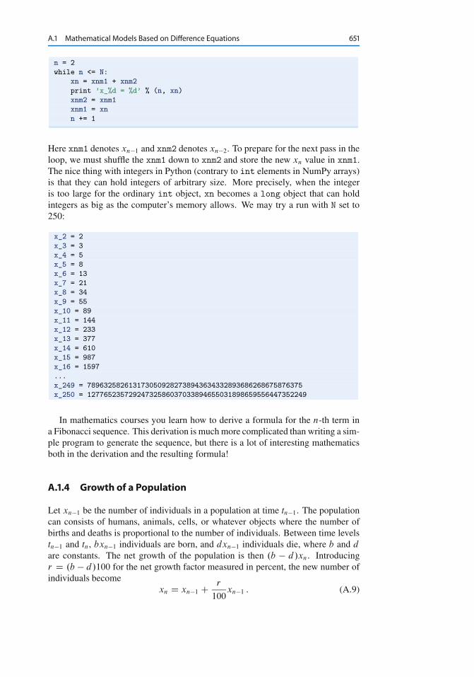
n = 2
while n <= N:
xn = xnm1 + xnm2
print ’x_%d = %d’ % (n, xn)
xnm2 = xnm1
xnm1 = xn
n += 1
Here xnm1 denotes xn�1 and xnm2 denotes xn�2. To prepare for the next pass in theloop, we must shuffle the xnm1 down to xnm2 and store the new xn value in xnm1.The nice thing with integers in Python (contrary to int elements in NumPy arrays)is that they can hold integers of arbitrary size. More precisely, when the integeris too large for the ordinary int object, xn becomes a long object that can holdintegers as big as the computer’s memory allows. We may try a run with N set to250:
x_2 = 2
x_3 = 3
x_4 = 5
x_5 = 8
x_6 = 13
x_7 = 21
x_8 = 34
x_9 = 55
x_10 = 89
x_11 = 144
x_12 = 233
x_13 = 377
x_14 = 610
x_15 = 987
x_16 = 1597
...
x_249 = 7896325826131730509282738943634332893686268675876375
x_250 = 12776523572924732586037033894655031898659556447352249
In mathematics courses you learn how to derive a formula for the n-th term ina Fibonacci sequence. This derivation is much more complicated than writing a sim-ple program to generate the sequence, but there is a lot of interesting mathematicsboth in the derivation and the resulting formula!
A.1.4 Growth of a Population
Let xn�1 be the number of individuals in a population at time tn�1. The populationcan consists of humans, animals, cells, or whatever objects where the number ofbirths and deaths is proportional to the number of individuals. Between time levelstn�1 and tn, bxn�1 individuals are born, and dxn�1 individuals die, where b and d
are constants. The net growth of the population is then .b � d/xn. Introducingr D .b � d/100 for the net growth factor measured in percent, the new number ofindividuals become
xn D xn�1 C r
100xn�1 : (A.9)
652 A Sequences and Difference Equations
This is the same difference equation as (A.5). It models growth of populations quitewell as long as there are optimal growing conditions for each individual. If not, onecan adjust the model as explained in Sect. A.1.5.
To solve (A.9) we need to start out with a known size x0 of the population. Theb and d parameters depend on the time difference tn � tn�1, i.e., the values of b andd are smaller if n counts years than if n counts generations.
A.1.5 Logistic Growth
The model (A.9) for the growth of a population leads to exponential increase in thenumber of individuals as implied by the solution (A.4). The size of the populationincreases faster and faster as time n increases, and xn ! 1 when n ! 1. In reallife, however, there is an upper limit M of the number of individuals that can existin the environment at the same time. Lack of space and food, competition betweenindividuals, predators, and spreading of contagious diseases are examples on factorsthat limit the growth. The number M is usually called the carrying capacity of theenvironment, the maximum population which is sustainable over time. With limitedgrowth, the growth factor r must depend on time:
xn D xn�1 C r.n � 1/
100xn�1 : (A.10)
In the beginning of the growth process, there is enough resources and the growthis exponential, but as xn approaches M , the growth stops and r must tend to zero.A simple function r.n/ with these properties is
r.n/ D %�1 � xn
M
�: (A.11)
For small n, xn � M and r.n/ � %, which is the growth rate with unlimitedresources. As n ! M , r.n/ ! 0 as we want. The model (A.11) is used for logisticgrowth. The corresponding logistic difference equation becomes
xn D xn�1 C %
100xn�1
�1 � xn�1
M
�: (A.12)
Below is a program (growth_logistic.py) for simulating N D 200 time inter-vals in a case where we start with x0 D 100 individuals, a carrying capacity ofM D 500, and initial growth of % D 4 percent in each time interval:
from scitools.std import *
x0 = 100 # initial amount of individuals
M = 500 # carrying capacity
rho = 4 # initial growth rate in percent
N = 200 # number of time intervals
index_set = range(N+1)
x = zeros(len(index_set))
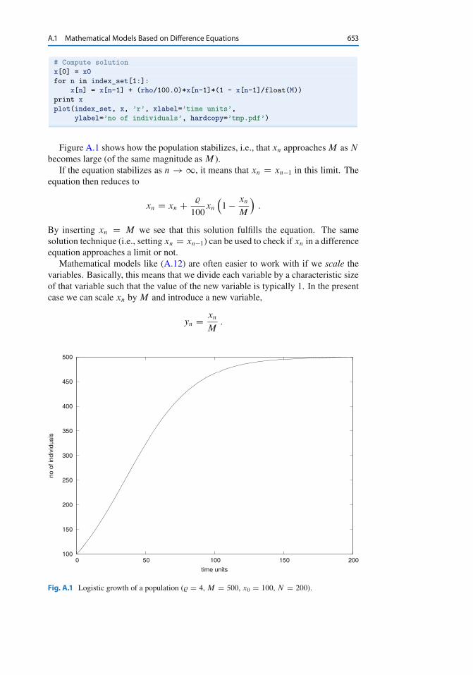
A.1 Mathematical Models Based on Difference Equations 653
# Compute solution
x[0] = x0
for n in index_set[1:]:
x[n] = x[n-1] + (rho/100.0)*x[n-1]*(1 - x[n-1]/float(M))
print x
plot(index_set, x, ’r’, xlabel=’time units’,
ylabel=’no of individuals’, hardcopy=’tmp.pdf’)
Figure A.1 shows how the population stabilizes, i.e., that xn approaches M as N
becomes large (of the same magnitude as M ).If the equation stabilizes as n ! 1, it means that xn D xn�1 in this limit. The
equation then reduces to
xn D xn C %
100xn
�1 � xn
M
�:
By inserting xn D M we see that this solution fulfills the equation. The samesolution technique (i.e., setting xn D xn�1) can be used to check if xn in a differenceequation approaches a limit or not.
Mathematical models like (A.12) are often easier to work with if we scale thevariables. Basically, this means that we divide each variable by a characteristic sizeof that variable such that the value of the new variable is typically 1. In the presentcase we can scale xn by M and introduce a new variable,
yn D xn
M:
100
150
200
250
300
350
400
450
500
0 50 100 150 200
no o
f ind
ivid
uals
time units
Fig. A.1 Logistic growth of a population (% D 4, M D 500, x0 D 100, N D 200).
654 A Sequences and Difference Equations
Similarly, x0 is replaced by y0 D x0=M . Inserting xn D Myn in (A.12) anddividing by M gives
yn D yn�1 C qyn�1 .1 � yn�1/ ; (A.13)
where q D %=100 is introduced to save typing. Equation (A.13) is simpler than(A.12) in that the solution lies approximately between y0 and 1 (values larger than1 can occur, see Exercise A.19), and there are only two dimensionless input pa-rameters to care about: q and y0. To solve (A.12) we need knowledge of threeparameters: x0, %, and M .
A.1.6 Payback of a Loan
A loan L is to be paid back over N months. The payback in a month consists of thefraction L=N plus the interest increase of the loan. Let the annual interest rate forthe loan be p percent. The monthly interest rate is then p
12. The value of the loan
after month n is xn, and the change from xn�1 can be modeled as
xn D xn�1 C p
12 � 100xn�1 �
�p
12 � 100xn�1 C L
N
�; (A.14)
D xn�1 � L
N; (A.15)
for n D 1; : : : ; N . The initial condition is x0 D L. A major difference between(A.15) and (A.6) is that all terms in the latter are proportional to xn or xn�1, while(A.15) also contains a constant term (L=N ). We say that (A.6) is homogeneous andlinear, while (A.15) is inhomogeneous (because of the constant term) and linear.The mathematical solution of inhomogeneous equations are more difficult to findthan the solution of homogeneous equations, but in a program there is no big differ-ence: we just add the extra term �L=N in the formula for the difference equation.
The solution of (A.15) is not particularly exciting (just use (A.15) repeatedly toderive the solution xn D L � nL=N ). What is more interesting, is what we payeach month, yn. We can keep track of both yn and xn in a variant of the previousmodel:
yn D p
12 � 100xn�1 C L
N; (A.16)
xn D xn�1 C p
12 � 100xn�1 � yn : (A.17)
Equations (A.16)–(A.17) is a system of difference equations. In a computer code,we simply update yn first, and then we update xn, inside a loop over n. Exercise A.4asks you to do this.
A.1 Mathematical Models Based on Difference Equations 655
A.1.7 The Integral as a Difference Equation
Suppose a function f .x/ is defined as the integral
f .x/ DxZ
a
g.t/dt : (A.18)
Our aim is to evaluate f .x/ at a set of points x0 D a < x1 < � � � < xN . Thevalue f .xn/ for any 0 � n � N can be obtained by using the Trapezoidal rule forintegration:
f .xn/ Dn�1XkD0
1
2.xkC1 � xk/.g.xk/ C g.xkC1//; (A.19)
which is nothing but the sum of the areas of the trapezoids up to the point xn (theplot to the right in Fig. 5.22 illustrates the idea.) We realize that f .xnC1/ is the sumabove plus the area of the next trapezoid:
f .xnC1/ D f .xn/ C 1
2.xnC1 � xn/.g.xn/ C g.xnC1// : (A.20)
This is a much more efficient formula than using (A.19) with n replaced by n C 1,since we do not need to recompute the areas of the first n trapezoids.
Formula (A.20) gives the idea of computing all the f .xn/ values through a differ-ence equation. Define fn as f .xn/ and consider x0 D a, and x1; : : : ; xN as given.We know that f0 D 0. Then
fn D fn�1 C 1
2.xn � xn�1/.g.xn�1/ C g.xn//; (A.21)
for n D 1; 2; : : : ; N . By introducing gn for g.xn/ as an extra variable in the differ-ence equation, we can avoid recomputing g.xn/ when we compute fnC1:
gn D g.xn/; (A.22)
fn D fn�1 C 1
2.xn � xn�1/.gn�1 C gn/; (A.23)
with initial conditions f0 D 0 and g0 D g.a/.A function can take g, a, x, and N as input and return arrays x and f for
x0; : : : ; xN and the corresponding integral values f0; : : : ; fN :
def integral(g, a, x, N=20):
index_set = range(N+1)
x = np.linspace(a, x, N+1)
g_ = np.zeros_like(x)
f = np.zeros_like(x)
g_[0] = g(x[0])
f[0] = 0
for n in index_set[1:]:
g_[n] = g(x[n])
f[n] = f[n-1] + 0.5*(x[n] - x[n-1])*(g_[n-1] + g_[n])
return x, f
656 A Sequences and Difference Equations
Note that g is used for the integrand function to call so we introduce g_ to be thearray holding sequence of g(x[n]) values.
Our first task, after having implemented a mathematical calculation, is to verifythe result. Here we can make use of the nice fact that the Trapezoidal rule is exactfor linear functions g.t/:
def test_integral():
def g_test(t):
"""Linear integrand."""
return 2*t + 1
def f_test(x, a):
"""Exact integral of g_test."""
return x**2 + x - (a**2 + a)
a = 2
x, f = integral(g_test, a, x=10)
f_exact = f_test(x, a)
assert np.allclose(f_exact, f)
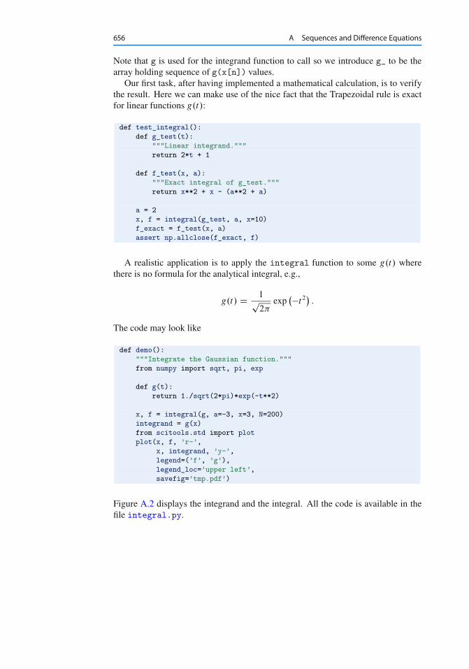
A realistic application is to apply the integral function to some g.t/ wherethere is no formula for the analytical integral, e.g.,
g.t/ D 1p2�
exp��t2
�:
The code may look like
def demo():
"""Integrate the Gaussian function."""
from numpy import sqrt, pi, exp
def g(t):
return 1./sqrt(2*pi)*exp(-t**2)
x, f = integral(g, a=-3, x=3, N=200)
integrand = g(x)
from scitools.std import plot
plot(x, f, ’r-’,
x, integrand, ’y-’,
legend=(’f’, ’g’),
legend_loc=’upper left’,
savefig=’tmp.pdf’)
Figure A.2 displays the integrand and the integral. All the code is available in thefile integral.py.

A.1 Mathematical Models Based on Difference Equations 657
0
0.1
0.2
0.3
0.4
0.5
0.6
0.7
0.8
-3 -2 -1 0 1 2 3
fg
Fig. A.2 Integral of 1p2�
exp��t 2
�from �3 to x.
A.1.8 Taylor Series as a Difference Equation
Consider the following system of two difference equations
en D en�1 C an�1; (A.24)
an D x
nan�1; (A.25)
with initial conditions e0 D 0 and a0 D 1. We can start to nest the solution:
e1 D 0 C a0 D 0 C 1 D 1;
a1 D x;
e2 D e1 C a1 D 1 C x;
a2 D x
2a1 D x2
2;
e3 D e2 C a2 D 1 C x C x2
2;
e4 D 1 C x C x2
2C x3
3 � 2;
e5 D 1 C x C x2
2C x3
3 � 2C x4
4 � 3 � 2
The observant reader who has heard about Taylor series (see Sect. B.4) will recog-nize this as the Taylor series of ex :
ex D1X
nD0
xn
nŠ: (A.26)
How do we derive a system like (A.24)–(A.25) for computing the Taylor poly-nomial approximation to ex? The starting point is the sum
P1nD0
xn
nŠ. This sum is
658 A Sequences and Difference Equations
coded by adding new terms to an accumulation variable in a loop. The mathematicalcounterpart to this code is a difference equation
enC1 D en C xn
nŠ; e0 D 0; n D 0; 1; 2; : : : : (A.27)
or equivalently (just replace n by n � 1):
en D en�1 C xn�1
n � 1Š; e0 D 0; n D 1; 2; 3; : : : : (A.28)
Now comes the important observation: the term xn=nŠ contains many of the com-putations we already performed for the previous term xn�1=.n � 1/Š because
xn
nŠD x � x � � � x
n.n � 1/.n � 2/ � � � 1;xn�1
.n � 1/ŠD x � x � � � x
.n � 1/.n � 2/.n � 3/ � � � 1 :
Let an D xn=nŠ. We see that we can go from an�1 to an by multiplying an�1 byx=n:
x
nan�1 D x
n
xn�1
.n � 1/ŠD xn
nŠD an; (A.29)
which is nothing but (A.25). We also realize that a0 D 1 is the initial condition forthis difference equation. In other words, (A.24) sums the Taylor polynomial, and(A.25) updates each term in the sum.
The system (A.24)–(A.25) is very easy to implement in a program and consti-tutes an efficient way to compute (A.26). The function exp_diffeq does the work:
def exp_diffeq(x, N):
n = 1
an_prev = 1.0 # a_0
en_prev = 0.0 # e_0
while n <= N:
en = en_prev + an_prev
an = x/n*an_prev
en_prev = en
an_prev = an
n += 1
return en
Observe that we do not store the sequences in arrays, but make use of the factthat only the most recent sequence element is needed to calculate a new element.The above function along with a direct evaluation of the Taylor series for ex anda comparison with the exact result for various N values can be found in the fileexp_Taylor_series_diffeq.py.
A.1.9 Making a Living from a Fortune
Suppose you want to live on a fortune F . You have invested the money in a safeway that gives an annual interest of p percent. Every year you plan to consume an
A.1 Mathematical Models Based on Difference Equations 659
amount cn, where n counts years. The development of your fortune xn from oneyear to the other can then be modeled by
xn D xn�1 C p
100xn�1 � cn�1; x0 D F : (A.30)
A simple example is to keep c constant, say q percent of the interest the first year:
xn D xn�1 C p
100xn�1 � pq
104F; x0 D F : (A.31)
A more realistic model is to assume some inflation of I percent per year. You willthen like to increase cn by the inflation. We can extend the model in two ways. Thesimplest and clearest way, in the author’s opinion, is to track the evolution of twosequences xn and cn:
xn D xn�1 C p
100xn�1 � cn�1; x0 D F; c0 D pq
104F; (A.32)
cn D cn�1 C I
100cn�1 : (A.33)
This is a system of two difference equations with two unknowns. The solutionmethod is, nevertheless, not much more complicated than the method for a differ-ence equation in one unknown, since we can first compute xn from (A.32) and thenupdate the cn value from (A.33). You are encouraged to write the program (seeExercise A.5).
Another way of making a difference equation for the case with inflation, is to usean explicit formula for cn�1, i.e., solve (A.32) and end up with a formula like (A.4).Then we can insert the explicit formula
cn�1 D�
1 C I
100
�n�1pq
104F
in (A.30), resulting in only one difference equation to solve.
A.1.10 Newton’s Method
The difference equation
xn D xn�1 � f .xn�1/
f 0.xn�1/; x0 given; (A.34)
generates a sequence xn where, if the sequence converges (i.e., if xn � xn�1 ! 0),xn approaches a root of f .x/. That is, xn ! x, where x solves the equationf .x/ D 0. Equation (A.34) is the famous Newton’s method for solving nonlinearalgebraic equations f .x/ D 0. When f .x/ is not linear, i.e., f .x/ is not on the formax C b with constant a and b, (A.34) becomes a nonlinear difference equation.This complicates analytical treatment of difference equations, but poses no extradifficulties for numerical solution.
660 A Sequences and Difference Equations
We can quickly sketch the derivation of (A.34). Suppose we want to solve theequation
f .x/ D 0
and that we already have an approximate solution xn�1. If f .x/ were linear, f .x/ Dax C b, it would be very easy to solve f .x/ D 0: x D �b=a. The idea is thereforeto approximate f .x/ in the vicinity of x D xn�1 by a linear function, i.e., a straightline f .x/ � Qf .x/ D ax C b. This line should have the same slope as f .x/, i.e.,a D f 0.xn�1/, and both the line and f should have the same value at x D xn�1.From this condition one can find b D f .xn�1/ � xn�1f
0.xn�1/. The approximatefunction (line) is then
Qf .x/ D f .xn�1/ C f 0.xn�1/.x � xn�1/ : (A.35)
This expression is just the two first terms of a Taylor series approximation to f .x/
at x D xn�1. It is now easy to solve Qf .x/ D 0 with respect to x, and we get
x D xn�1 � f .xn�1/
f 0.xn�1/: (A.36)
Since Qf is only an approximation to f , x in (A.36) is only an approximation toa root of f .x/ D 0. Hopefully, the approximation is better than xn�1 so we setxn D x as the next term in a sequence that we hope converges to the correct root.However, convergence depends highly on the shape of f .x/, and there is no guar-antee that the method will work.
The previous programs for solving difference equations have typically calculateda sequence xn up to n D N , where N is given. When using (A.34) to find rootsof nonlinear equations, we do not know a suitable N in advance that leads to an xn
where f .xn/ is sufficiently close to zero. We therefore have to keep on increasingn until f .xn/ < � for some small �. Of course, the sequence diverges, we will keepon forever, so there must be some maximum allowable limit on n, which we maytake as N .
It can be convenient to have the solution of (A.34) as a function for easy reuse.Here is a first rough implementation:
def Newton(f, x, dfdx, epsilon=1.0E-7, N=100):
n = 0
while abs(f(x)) > epsilon and n <= N:
x = x - f(x)/dfdx(x)
n += 1
return x, n, f(x)
This function might well work, but f(x)/dfdx(x) can imply integer division, sowe should ensure that the numerator or denumerator is of float type. There arealso two function evaluations of f(x) in every pass in the loop (one in the loop bodyand one in the while condition). We can get away with only one evaluation if westore the f(x) in a local variable. In the small examples with f .x/ in the presentcourse, twice as many function evaluations of f as necessary does not matter, butthe same Newton function can in fact be used for much more complicated functions,
A.1 Mathematical Models Based on Difference Equations 661
and in those cases twice as much work can be noticeable. As a programmer, youshould therefore learn to optimize the code by removing unnecessary computations.
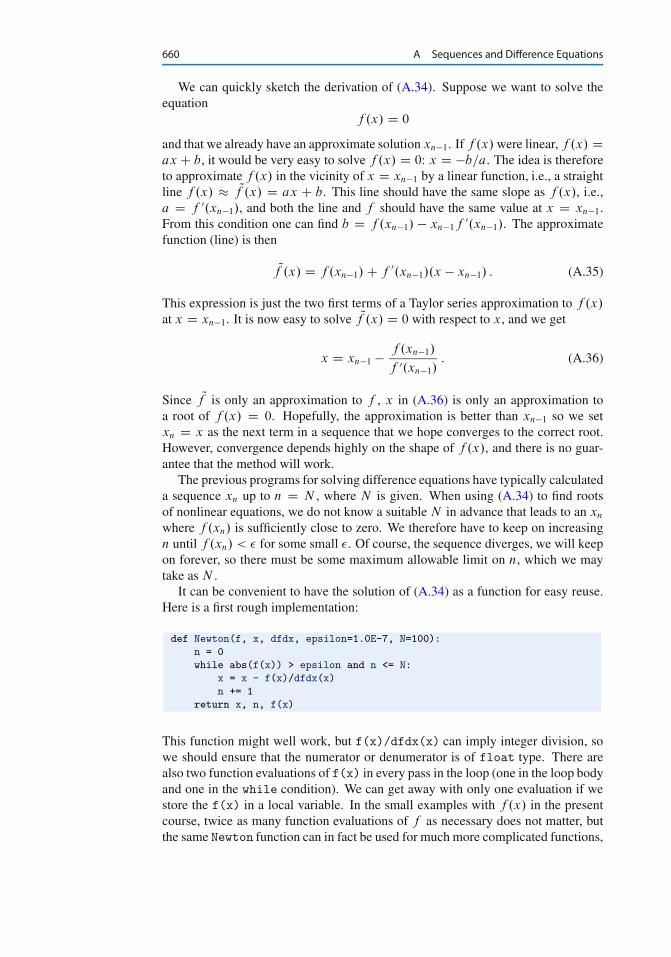
Another, more serious, problem is the possibility dividing by zero. Almost asserious, is dividing by a very small number that creates a large value, which mightcause Newton’s method to diverge. Therefore, we should test for small values off 0.x/ and write a warning or raise an exception.
Another improvement is to add a boolean argument store to indicate whetherwe want the .x; f .x// values during the iterations to be stored in a list or not. Theseintermediate values can be handy if we want to print out or plot the convergencebehavior of Newton’s method.
An improved Newton function can now be coded as
def Newton(f, x, dfdx, epsilon=1.0E-7, N=100, store=False):
f_value = f(x)
n = 0
if store: info = [(x, f_value)]
while abs(f_value) > epsilon and n <= N:
dfdx_value = float(dfdx(x))
if abs(dfdx_value) < 1E-14:
raise ValueError("Newton: f’(%g)=%g" % (x, dfdx_value))
x = x - f_value/dfdx_value
n += 1
f_value = f(x)
if store: info.append((x, f_value))
if store:
return x, info
else:
return x, n, f_value
Note that to use the Newton function, we need to calculate the derivative f 0.x/
and implement it as a Python function and provide it as the dfdx argument. Alsonote that what we return depends on whether we store .x; f .x// information duringthe iterations or not.
It is quite common to test if dfdx(x) is zero in an implementation of New-ton’s method, but this is not strictly necessary in Python since an exceptionZeroDivisionError is always raised when dividing by zero.
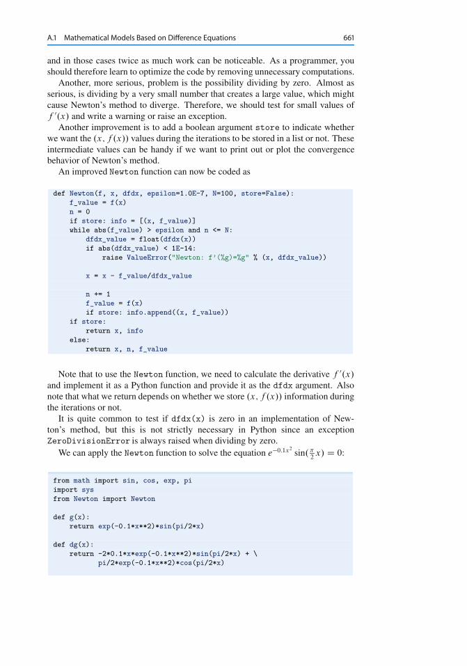
We can apply the Newton function to solve the equation e�0:1x2sin.�
2x/ D 0:
from math import sin, cos, exp, pi
import sys
from Newton import Newton
def g(x):
return exp(-0.1*x**2)*sin(pi/2*x)
def dg(x):
return -2*0.1*x*exp(-0.1*x**2)*sin(pi/2*x) + \
pi/2*exp(-0.1*x**2)*cos(pi/2*x)
662 A Sequences and Difference Equations
x0 = float(sys.argv[1])
x, info = Newton(g, x0, dg, store=True)
print ’root:’, x
for i in range(len(info)):
print ’Iteration %3d: f(%g)=%g’ % \
(i, info[i][0], info[i][1])
The Newton function and this program can be found in the file Newton.py. Run-ning this program with an initial x value of 1.7 results in the output
root: 1.999999999768449
Iteration 0: f(1.7)=0.340044
Iteration 1: f(1.99215)=0.00828786
Iteration 2: f(1.99998)=2.53347e-05
Iteration 3: f(2)=2.43808e-10
Fortunately you realize that the exponential function can never be zero, so the so-lutions of the equation must be the zeros of the sine function, i.e., �
2x D i� for
all integers i D : : : ; �2; 1; 0; 1; 2; : : :. This gives x D 2i as the solutions. We seefrom the output that the convergence is fast towards the solution x D 2. The erroris of the order 10�10 even though we stop the iterations when f .x/ � 10�7.
Trying a start value of 3, we would expect the method to find the root x D 2 orx D 4, but now we get
root: 42.49723316011362
Iteration 0: f(3)=-0.40657
Iteration 1: f(4.66667)=0.0981146
Iteration 2: f(42.4972)=-2.59037e-79
We have definitely solved f .x/ D 0 in the sense that jf .x/j � �, where � is a smallvalue (here � � 10�79). However, the solution x � 42:5 is not close to the correctsolution (x D 42 and x D 44 are the solutions closest to the computed x). Can youuse your knowledge of how the Newton method works and figure out why we getsuch strange behavior?
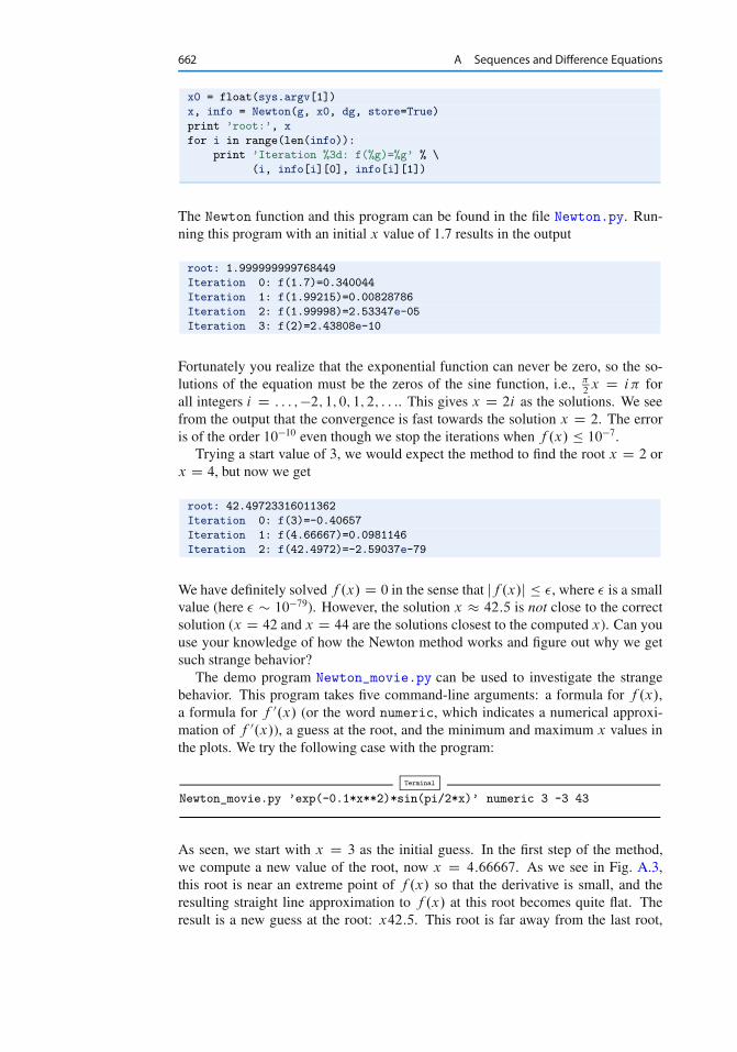
The demo program Newton_movie.py can be used to investigate the strangebehavior. This program takes five command-line arguments: a formula for f .x/,a formula for f 0.x/ (or the word numeric, which indicates a numerical approxi-mation of f 0.x/), a guess at the root, and the minimum and maximum x values inthe plots. We try the following case with the program:
Terminal
Newton_movie.py ’exp(-0.1*x**2)*sin(pi/2*x)’ numeric 3 -3 43
As seen, we start with x D 3 as the initial guess. In the first step of the method,we compute a new value of the root, now x D 4:66667. As we see in Fig. A.3,this root is near an extreme point of f .x/ so that the derivative is small, and theresulting straight line approximation to f .x/ at this root becomes quite flat. Theresult is a new guess at the root: x42:5. This root is far away from the last root,
A.1 Mathematical Models Based on Difference Equations 663
-0.8
-0.6
-0.4
-0.2
0
0.2
0.4
0.6
0.8
0 5 10 15 20 25 30 35 40
approximate root = 4.66667; f(4.66667) = 0.0981146
f(x)approx. rootapprox. line
Fig. A.3 Failure of Newton’s method to solve e�0:1x2sin. �
2x/ D 0. The plot corresponds to the
second root found (starting with x D 3).
but the second problem is that f .x/ is quickly damped as we move to increasing x
values, and at x D 42:5 f is small enough to fulfill the convergence criterion. Anyguess at the root out in this region would satisfy that criterion.
You can run the Newton_movie.py program with other values of the initial rootand observe that the method usually finds the nearest roots.
A.1.11 The Inverse of a Function
Given a function f .x/, the inverse function of f , say we call it g.x/, has the prop-erty that if we apply g to the value f .x/, we get x back:
g.f .x// D x :
Similarly, if we apply f to the value g.x/, we get x:
f .g.x// D x : (A.37)
By hand, you substitute g.x/ by (say) y in (A.37) and solve (A.37) with respect toy to find some x expression for the inverse function. For example, given f .x/ Dx2 � 1, we must solve y2 � 1 D x with respect to y. To ensure a unique solutionfor y, the x values have to be limited to an interval where f .x/ is monotone, sayx 2 Œ0; 1� in the present example. Solving for y gives y D p
1 C x, thereforeg.x/ D p
1 C x. It is easy to check that f .g.x// D .p
1 C x/2 � 1 D x.
664 A Sequences and Difference Equations
Numerically, we can use the “definition” (A.37) of the inverse function g at onepoint at a time. Suppose we have a sequence of points x0 < x1 < � � � < xN alongthe x axis such that f is monotone in Œx0; xN �: f .x0/ > f .x1/ > � � � > f .xN / orf .x0/ < f .x1/ < � � � < f .xN /. For each point xi , we have
f .g.xi // D xi :
The value g.xi / is unknown, so let us call it � . The equation
f .�/ D xi (A.38)
can be solved be respect � . However, (A.38) is in general nonlinear if f is a non-linear function of x. We must then use, e.g., Newton’s method to solve (A.38).Newton’s method works for an equation phrased as f .x/ D 0, which in our caseis f .�/ � xi D 0, i.e., we seek the roots of the function F.�/ f .�/ � xi . Alsothe derivative F 0.�/ is needed in Newton’s method. For simplicity we may use anapproximate finite difference:
dF
d�� F.� C h/ � F.� � h/
2h:
As start value �0, we can use the previously computed g value: gi�1. We introducethe short notation � D Newton.F; �0/ to indicate the solution of F.�/ D 0 withinitial guess �0.
The computation of all the g0; : : : ; gN values can now be expressed by
gi D Newton.F; gi�1/; i D 1; : : : ; N; (A.39)
and for the first point we may use x0 as start value (for instance):
g0 D Newton.F; x0/ : (A.40)
Equations (A.39)–(A.40) constitute a difference equation for gi , since given gi�1,we can compute the next element of the sequence by (A.39). Because (A.39) isa nonlinear equation in the new value gi , and (A.39) is therefore an example ofa nonlinear difference equation.
The following program computes the inverse function g.x/ of f .x/ at somediscrete points x0; : : : ; xN . Our sample function is f .x/ D x2 � 1:
from Newton import Newton
from scitools.std import *
def f(x):
return x**2 - 1
def F(gamma):
return f(gamma) - xi
A.2 Programmingwith Sound 665
def dFdx(gamma):
return (F(gamma+h) - F(gamma-h))/(2*h)
h = 1E-6
x = linspace(0.01, 3, 21)
g = zeros(len(x))
for i in range(len(x)):
xi = x[i]
# Compute start value (use last g[i-1] if possible)
if i == 0:
gamma0 = x[0]
else:
gamma0 = g[i-1]
gamma, n, F_value = Newton(F, gamma0, dFdx)
g[i] = gamma
plot(x, f(x), ’r-’, x, g, ’b-’,
title=’f1’, legend=(’original’, ’inverse’))
Note that with f .x/ D x2 � 1, f 0.0/ D 0, so Newton’s method divides by zeroand breaks down unless with let x0 > 0, so here we set x0 D 0:01. The f functioncan easily be edited to let the program compute the inverse of another function.The F function can remain the same since it applies a general finite difference toapproximate the derivative of the f(x) function. The complete program is found inthe file inverse_function.py.
A.2 Programming with Sound
Sound on a computer is nothing but a sequence of numbers. As an example, con-sider the famous A tone at 440Hz. Physically, this is an oscillation of a tuning fork,loudspeaker, string or another mechanical medium that makes the surrounding airalso oscillate and transport the sound as a compression wave. This wave may hit ourears and through complicated physiological processes be transformed to an electri-cal signal that the brain can recognize as sound. Mathematically, the oscillationsare described by a sine function of time:
s.t/ D A sin .2�f t/ ; (A.41)
where A is the amplitude or strength of the sound and f is the frequency (440Hzfor the A in our example). In a computer, s.t/ is represented at discrete points oftime. CD quality means 44100 samples per second. Other sample rates are alsopossible, so we introduce r as the sample rate. An f Hz tone lasting for m secondswith sample rate r can then be computed as the sequence
sn D A sin�2�f
n
r
�; n D 0; 1; : : : ; m � r : (A.42)
666 A Sequences and Difference Equations
With Numerical Python this computation is straightforward and very efficient. In-troducing some more explanatory variable names than r , A, and m, we can writea function for generating a note:
import numpy as np
def note(frequency, length, amplitude=1, sample_rate=44100):
time_points = np.linspace(0, length, length*sample_rate)
data = np.sin(2*np.pi*frequency*time_points)
data = amplitude*data
return data
A.2.1 Writing Sound to File
The note function above generates an array of float data representing a note. Thesound card in the computer cannot play these data, because the card assumes thatthe information about the oscillations appears as a sequence of two-byte integers.With an array’s astypemethod we can easily convert our data to two-byte integersinstead of floats:
data = data.astype(numpy.int16)
That is, the name of the two-byte integer data type in numpy is int16 (two bytesare 16 bits). The maximum value of a two-byte integer is 215 � 1, so this is also themaximum amplitude. Assuming that amplitude in the note function is a relativemeasure of intensity, such that the value lies between 0 and 1, we must adjust thisamplitude to the scale of two-byte integers:
max_amplitude = 2**15 - 1
data = max_amplitude*data
The data array of int16 numbers can be written to a file and played as an or-dinary file in CD quality. Such a file is known as a wave file or simply a WAVfile since the extension is .wav. Python has a module wave for creating such files.Given an array of sound, data, we have in SciTools a module sound with a func-tion write for writing the data to a WAV file (using functionality from the wavemodule):
import scitools.sound
scitools.sound.write(data, ’Atone.wav’)
You can now use your favorite music player to play the Atone.wav file, or you canplay it from within a Python program using
scitools.sound.play(’Atone.wav’)
The write function can take more arguments and write, e.g., a stereo file with twochannels, but we do not dive into these details here.
A.2 Programmingwith Sound 667
A.2.2 Reading Sound from File
Given a sound signal in a WAV file, we can easily read this signal into an arrayand mathematically manipulate the data in the array to change the flavor of thesound, e.g., add echo, treble, or bass. The recipe for reading a WAV file with namefilename is
data = scitools.sound.read(filename)
The data array has elements of type int16. Often we want to compute with thisarray, and then we need elements of float type, obtained by the conversion
data = data.astype(float)
The write function automatically transforms the element type back to int16 if wehave not done this explicitly.
One operation that we can easily do is adding an echo. Mathematically thismeans that we add a damped delayed sound, where the original sound has weight ˇ
and the delayed part has weight 1�ˇ, such that the overall amplitude is not altered.Let d be the delay in seconds. With a sampling rate r the number of indices in thedelay becomes dr , which we denote by b. Given an original sound sequence sn, thesound with echo is the sequence
en D ˇsn C .1 � ˇ/sn�b : (A.43)
We cannot start n at 0 since e0 D s0�b D s�b which is a value outside the sounddata. Therefore we define en D sn for n D 0; 1; : : : ; b, and add the echo thereafter.A simple loop can do this (again we use descriptive variable names instead of themathematical symbols introduced):
def add_echo(data, beta=0.8, delay=0.002, sample_rate=44100):
newdata = data.copy()
shift = int(delay*sample_rate) # b (math symbol)
for i in range(shift, len(data)):
newdata[i] = beta*data[i] + (1-beta)*data[i-shift]
return newdata
The problemwith this function is that it runs slowly, especially when we have soundclips lasting several seconds (recall that for CD quality we need 44100 numbers persecond). It is therefore necessary to vectorize the implementation of the differenceequation for adding echo. The update is then based on adding slices:
newdata[shift:] = beta*data[shift:] + \
(1-beta)*data[:len(data)-shift]
A.2.3 Playing Many Notes
How do we generate a melody mathematically in a computer program? With thenote function we can generate a note with a certain amplitude, frequency, and
668 A Sequences and Difference Equations
duration. The note is represented as an array. Putting sound arrays for differentnotes after each other will make up a melody. If we have several sound arraysdata1, data2, data3, : : :, we can make a new array consisting of the elements inthe first array followed by the elements of the next array followed by the elementsin the next array and so forth:
data = numpy.concatenate((data1, data2, data3, ...))
The frequency of a note4 that is h half tones up from a base frequency f is givenby f 2h=12. With the tone A at 440Hz, we can define notes and the correspondingfrequencies as
base_freq = 440.0
notes = [’A’, ’A#’, ’B’, ’C’, ’C#’, ’D’, ’D#’, ’E’,
’F’, ’F#’, ’G’, ’G#’]
notes2freq = {notes[i]: base_freq*2**(i/12.0)
for i in range(len(notes))}
With the notes to frequency mapping a melody can be made as a series of noteswith specified duration:
l = .2 # basic duration unit
tones = [(’E’, 3*l), (’D’, l), (’C#’, 2*l), (’B’, 2*l), (’A’, 2*l),
(’B’, 2*l), (’C#’, 2*l), (’D’, 2*l), (’E’, 3*l),
(’F#’, l), (’E’, 2*l), (’D’, 2*l), (’C#’, 4*l)]
samples = []
for tone, duration in tones :
s = note(notes2freq[tone], duration)
samples.append(s)
data = np.concatenate(samples)
data *= 2**15-1
scitools.sound.write(data, "melody.wav")
Playing the resulting file melody.wav reveals that this is the opening of the most-played tune during international cross country skiing competitions.
All the notes had the same amplitude in this example, but more dynamics caneasily be added by letting the elements in tones be triplets with tone, duration, andamplitude. The basic code above is found in the file melody.py.
A.2.4 Music of a Sequence
Problem The purpose of this example is to listen to the sound generated by twomathematical sequences. The first one is given by an explicit formula, constructedto oscillate around 0 with decreasing amplitude:
xn D e�4n=N sin.8�n=N / : (A.44)
4 http://en.wikipedia.org/wiki/Note
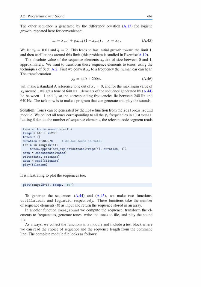
A.2 Programmingwith Sound 669
The other sequence is generated by the difference equation (A.13) for logisticgrowth, repeated here for convenience:
xn D xn�1 C qxn�1 .1 � xn�1/ ; x D x0 : (A.45)
We let x0 D 0:01 and q D 2. This leads to fast initial growth toward the limit 1,and then oscillations around this limit (this problem is studied in Exercise A.19).
The absolute value of the sequence elements xn are of size between 0 and 1,approximately. We want to transform these sequence elements to tones, using thetechniques of Sect. A.2. First we convert xn to a frequency the human ear can hear.The transformation
yn D 440 C 200xn (A.46)
will make a standard A reference tone out of xn D 0, and for the maximum value ofxn around 1 we get a tone of 640Hz. Elements of the sequence generated by (A.44)lie between �1 and 1, so the corresponding frequencies lie between 240Hz and640Hz. The task now is to make a program that can generate and play the sounds.
Solution Tones can be generated by the note function from the scitools.soundmodule. We collect all tones corresponding to all the yn frequencies in a list tones.Letting N denote the number of sequence elements, the relevant code segment reads
from scitools.sound import *
freqs = 440 + x*200
tones = []
duration = 30.0/N # 30 sec sound in total
for n in range(N+1):
tones.append(max_amplitude*note(freqs[n], duration, 1))
data = concatenate(tones)
write(data, filename)
data = read(filename)
play(filename)
It is illustrating to plot the sequences too,
plot(range(N+1), freqs, ’ro’)
To generate the sequences (A.44) and (A.45), we make two functions,oscillations and logistic, respectively. These functions take the numberof sequence elements (N) as input and return the sequence stored in an array.
In another function make_sound we compute the sequence, transform the el-ements to frequencies, generate tones, write the tones to file, and play the soundfile.
As always, we collect the functions in a module and include a test block wherewe can read the choice of sequence and the sequence length from the commandline. The complete module file looks as follows:
670 A Sequences and Difference Equations
from scitools.sound import *
from scitools.std import *
def oscillations(N):
x = zeros(N+1)
for n in range(N+1):
x[n] = exp(-4*n/float(N))*sin(8*pi*n/float(N))
return x
def logistic(N):
x = zeros(N+1)
x[0] = 0.01
q = 2
for n in range(1, N+1):
x[n] = x[n-1] + q*x[n-1]*(1 - x[n-1])
return x
def make_sound(N, seqtype):
filename = ’tmp.wav’
x = eval(seqtype)(N)
# Convert x values to frequences around 440
freqs = 440 + x*200
plot(range(N+1), freqs, ’ro’)
# Generate tones
tones = []
duration = 30.0/N # 30 sec sound in total
for n in range(N+1):
tones.append(max_amplitude*note(freqs[n], duration, 1))
data = concatenate(tones)
write(data, filename)
data = read(filename)
play(filename)
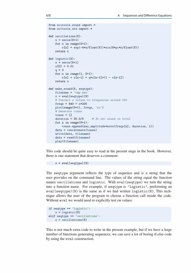
This code should be quite easy to read at the present stage in the book. However,there is one statement that deserves a comment:
x = eval(seqtype)(N)
The seqtype argument reflects the type of sequence and is a string that theuser provides on the command line. The values of the string equal the functionnames oscillations and logistic. With eval(seqtype) we turn the stringinto a function name. For example, if seqtype is ’logistic’, performing aneval(seqtype)(N) is the same as if we had written logistic(N). This tech-nique allows the user of the program to choose a function call inside the code.Without eval we would need to explicitly test on values:
if seqtype == ’logistic’:
x = logistic(N)
elif seqtype == ’oscillations’:
x = oscillations(N)
This is not much extra code to write in the present example, but if we have a largenumber of functions generating sequences, we can save a lot of boring if-else codeby using the eval construction.
A.3 Exercises 671
The next step, as a reader who have understood the problem and the implemen-tation above, is to run the program for two cases: the oscillations sequence withN D 40 and the logistic sequence with N D 100. By altering the q parameter tolower values, you get other sounds, typically quite boring sounds for non-oscillatinglogistic growth (q < 1). You can also experiment with other transformations of theform (A.46), e.g., increasing the frequency variation from 200 to 400.
A.3 Exercises
Exercise A.1: Determine the limit of a sequence
a) Write a Python function for computing and returning the sequence
an D 7 C 1=.n C 1/
3 � 1=.n C 1/2; n D 0; 2; : : : ; N :
Write out the sequence for N D 100. Find the exact limit as N ! 1 andcompare with aN .
b) Write a Python function for computing and returning the sequence
Dn D sin.2�n/
2�n; n D 0; : : : ; N :
Determine the limit of this sequence for large N .c) Given the sequence
Dn D f .x C h/ � f .x/
h; h D 2�n; (A.47)
make a function D(f, x, N) that takes a function f .x/, a value x, and thenumber N of terms in the sequence as arguments, and returns the sequence Dn
for n D 0; 1; : : : ; N . Make a call to the D function with f .x/ D sin x, x D 0,and N D 80. Plot the evolution of the computed Dn values, using small circlesfor the data points.
d) Make another call to D where x D � and plot this sequence in a separate figure.What would be your expected limit?
e) Explain why the computations for x D � go wrong for large N .
Hint Print out the numerator and denominator in Dn.Filename: sequence_limits.
672 A Sequences and Difference Equations
Exercise A.2: Compute � via sequencesThe following sequences all converge to � :
.an/1nD1; an D 4
nXkD1
.�1/kC1
2k � 1;
.bn/1nD1; bn D
6
nXkD1
k�2
!1=2
;
.cn/1nD1; cn D
90
nXkD1
k�4
!1=4
;
.dn/1nD1; dn D 6p
3
nXkD0
.�1/k
3k.2k C 1/;
.en/1nD1; en D 16
nXkD0
.�1/k
52kC1.2k C 1/� 4
nXkD0
.�1/k
2392kC1.2k C 1/:
Make a function for each sequence that returns an array with the elements in thesequence. Plot all the sequences, and find the one that converges fastest toward thelimit � .Filename: pi_sequences.
Exercise A.3: Reduce memory usage of difference equationsConsider the program growth_years.py from Sect. A.1.1. Since xn depends onxn�1 only, we do not need to store all the N C 1 xn values. We actually only needto store xn and its previous value xn�1. Modify the program to use two variablesand not an array for the entire sequence. Also avoid the index_set list and use aninteger counter for n and a while loop instead. Write the sequence to file such thatit can be visualized later.Filename: growth_years_efficient.
Exercise A.4: Compute the development of a loanSolve (A.16)–(A.17) in a Python function.Filename: loan.
Exercise A.5: Solve a system of difference equationsSolve (A.32)–(A.33) in a Python function and plot the xn sequence.Filename: fortune_and_inflation1.
Exercise A.6: Modify a model for fortune developmentIn the model (A.32)–(A.33) the new fortune is the old one, plus the interest, minusthe consumption. During year n, xn is normally also reduced with t percent tax onthe earnings xn�1 � xn�2 in year n � 1.
a) Extend the model with an appropriate tax term, implement the model, anddemonstrate in a plot the effect of tax (t D 27) versus no tax (t D 0).
A.3 Exercises 673
b) Suppose you expect to live for N years and can accept that the fortune xn van-ishes after N years. Choose some appropriate values for p, q, I , and t , andexperiment with the program to find how large the initial c0 can be in this case.
Filename: fortune_and_inflation2.
Exercise A.7: Change index in a difference equationA mathematically equivalent equation to (A.5) is
xiC1 D xi C p
100xi ; (A.48)
since the name of the index can be chosen arbitrarily. Suppose someone has madethe following program for solving (A.48):
from scitools.std import *
x0 = 100 # initial amount
p = 5 # interest rate
N = 4 # number of years
index_set = range(N+1)
x = zeros(len(index_set))
# Compute solution
x[0] = x0
for i in index_set[1:]:
x[i+1] = x[i] + (p/100.0)*x[i]
print x
plot(index_set, x, ’ro’, xlabel=’years’, ylabel=’amount’)
This program does not work. Make a correct version, but keep the difference equa-tions in its present form with the indices i+1 and i.Filename: growth1_index_ip1.
Exercise A.8: Construct time points from datesA certain quantity p (which may be an interest rate) is piecewise constant and un-dergoes changes at some specific dates, e.g.,
p changes to
8̂ˆ̂̂̂ˆ̂̂<ˆ̂̂̂ˆ̂̂̂:
4:5 on Jan 4, 2019
4:75 on March 21, 2019
6:0 on April 1, 2019
5:0 on June 30, 2019
4:5 on Nov 1, 2019
2:0 on April 1, 2020
(A.49)
Given a start date d1 and an end date d2, fill an array pwith the right p values, wherethe array index counts days. Use the datetimemodule to compute the number ofdays between dates.Filename: dates2days.
674 A Sequences and Difference Equations
Exercise A.9: Visualize the convergence of Newton’s methodLet x0; x1; : : : ; xN be the sequence of roots generated by Newton’s method appliedto a nonlinear algebraic equation f .x/ D 0 (see Sect. A.1.10). In this exercise,the purpose is to plot the sequences .xn/N
nD0 and .jf .xn/j/NnD0 such that we can
understand how Newton’s method converges or diverges.
a) Make a general function
Newton_plot(f, x, dfdx, xmin, xmax, epsilon=1E-7)
for this purpose. The arguments f and dfdx are Python functions represent-ing the f .x/ function in the equation and its derivative f 0.x/, respectively.Newton’s method is run until jf .xN /j � �, and the � value is available asthe epsilon argument. The Newton_plot function should make three sepa-rate plots of f .x/, .xn/N
nD0, and .jf .xn/j/NnD0 on the screen and also save these
plots to PNG files. The relevant x interval for plotting of f .x/ is given by thearguments xmin and xmax. Because of the potentially wide scale of values thatjf .xn/j may exhibit, it may be wise to use a logarithmic scale on the y axis.
Hint You can save quite some coding by calling the improved Newton functionfrom Sect. A.1.10, which is available in the module file Newton.py.
b) Demonstrate the function on the equation x6 sin�x D 0, with � D 10�13. Trydifferent starting values for Newton’s method: x0 D �2:6; �1:2; 1:5; 1:7; 0:6.Compare the results with the exact solutions x D : : : ; �2 � 1; 0; 1; 2; : : :.
c) Use the Newton_plot function to explore the impact of the starting point x0
when solving the following nonlinear algebraic equations:
sin x D 0; (A.50)
x D sin x; (A.51)
x5 D sin x; (A.52)
x4 sin x D 0; (A.53)
x4 D 16; (A.54)
x10 D 1; (A.55)
tanhx D 0; (A.56)
tanhx D x10 : (A.57)
Hint Such an experimental investigation is conveniently recorded in an IPythonnotebook. See Sect. H.4 for a quick introduction to notebooks.Filename: Newton2.
Exercise A.10: Implement the secant methodNewton’s method (A.34) for solving f .x/ D 0 requires the derivative of the func-tion f .x/. Sometimes this is difficult or inconvenient. The derivative can beapproximated using the last two approximations to the root, xn�2 and xn�1:
f 0.xn�1/ � f .xn�1/ � f .xn�2/
xn�1 � xn�2
:
A.3 Exercises 675
Using this approximation in (A.34) leads to the Secant method:
xn D xn�1 � f .xn�1/.xn�1 � xn�2/
f .xn�1/ � f .xn�2/; x0; x1 given : (A.58)
Here n D 2; 3; : : :. Make a program that applies the Secant method to solve x5 Dsin x.Filename: Secant.
Exercise A.11: Test different methods for root findingMake a program for solving f .x/ D 0 by Newton’s method (Sect. A.1.10), theBisection method (Sect. 4.11.2), and the Secant method (Exercise A.10). For eachmethod, the sequence of root approximations should be written out (nicely format-ted) on the screen. Read f .x/, f 0.x/, a, b, x0, and x1 from the command line.Newton’s method starts with x0, the Bisection method starts with the interval Œa; b�,whereas the Secant method starts with x0 and x1.
Run the program for each of the equations listed in Exercise A.9d. You shouldfirst plot the f .x/ functions so you know how to choose x0, x1, a, and b in eachcase.Filename: root_finder_examples.
Exercise A.12: Make difference equations for the Midpoint ruleUse the ideas of Sect. A.1.7 to make a similar system of difference equations andcorresponding implementation for the Midpoint integration rule:
bZ
a
f .x/dx � h
n�1XiD0
f .a � 1
2h C ih/;
where h D .b � a/=n and n counts the number of function evaluations (i.e., rectan-gles that approximate the area under the curve).Filename: diffeq_midpoint.
Exercise A.13: Compute the arc length of a curveSometimes one wants to measure the length of a curve y D f .x/ for x 2 Œa; b�. Thearc length from f .a/ to some point f .x/ is denoted by s.x/ and defined through anintegral
s.x/ DxZ
a
p1 C Œf 0.�/�2d� : (A.59)
We can compute s.x/ via difference equations as explained in Sect. A.1.7.
a) Make a Python function arclength(f, a, b, n) that returns an array s withs.x/ values for n uniformly spaced coordinates x in Œa; b�. Here f(x) is thePython implementation of the function that defines the curve we want to com-pute the arc length of.
b) How can you verify that the arclength function works correctly? Constructtest case(s) and write corresponding test functions for automating the tests.
676 A Sequences and Difference Equations
Hint Check the implementation for curves with known arc length, e.g., a semi-circle and a straight line.
c) Apply the function to
f .x/ DxZ
�2
D 1p2�
e�4t2
dt; x 2 Œ�2; 2� :
Compute s.x/ and plot it together with f .x/.
Filename: arclength.
Exercise A.14: Find difference equations for computing sinx
The purpose of this exercise is to derive and implement difference equations forcomputing a Taylor polynomial approximation to sin x:
sin x � S.xI n/ DnX
j D0
.�1/j x2j C1
.2j C 1/Š: (A.60)
To compute S.xI n/ efficiently, write the sum as S.xI n/ D Pnj D0 aj , and derive
a relation between two consecutive terms in the series:
aj D � x2
.2j C 1/2jaj �1 : (A.61)
Introduce sj D S.xI j � 1/ and aj as the two sequences to compute. We haves0 D 0 and a0 D x.
a) Formulate the two difference equations for sj and aj .
Hint Section A.1.8 explains how this task and the associated programming can besolved for the Taylor polynomial approximation of ex .
b) Implement the system of difference equations in a function sin_Taylor(x, n),which returns snC1 and janC1j. The latter is the first neglected term in the sum(since snC1 D Pn
j D0 aj ) and may act as a rough measure of the size of the errorin the Taylor polynomial approximation.
c) Verify the implementation by computing the difference equations for n D 2
by hand (or in a separate program) and comparing with the output from thesin_Taylor function. Automate this comparison in a test function.
d) Make a table or plot of sn for various x and n values to illustrate that the accuracyof a Taylor polynomial (around x D 0) improves as n increases and x decreases.
Hint Be aware of the fact that sin_Taylor(x, n) can give extremely inaccurateapproximations to sin x if x is not sufficiently small and n sufficiently large. Ina plot you must therefore define the axis appropriately.Filename: sin_Taylor_series_diffeq.
A.3 Exercises 677
Exercise A.15: Find difference equations for computing cosx
Solve Exercise A.14 for the Taylor polynomial approximation to cosx. (The rele-vant expression for the Taylor series is easily found in a mathematics textbook orby searching on the Internet.)Filename: cos_Taylor_series_diffeq.
Exercise A.16: Make a guitar-like soundGiven start values x0; x1; : : : ; xp , the following difference equation is known tocreate guitar-like sound:
xn D 1
2.xn�p C xn�p�1/; n D p C 1; : : : ; N : (A.62)
With a sampling rate r , the frequency of this sound is given by r=p. Make a programwith a function solve(x, p) which returns the solution array x of (A.62). Toinitialize the array x[0:p+1] we look at two methods, which can be implementedin two alternative functions:
x0 D 1, x1 D x2 D � � � D xp D 0
x0; : : : ; xp are uniformly distributed random numbers in Œ�1; 1�
Import max_amplitude, write, and play from the scitools.sound module.Choose a sampling rate r and set p D r=440 to create a 440Hz tone (A). Createan array x1 of zeros with length 3r such that the tone will last for 3 seconds. Ini-tialize x1 according to method 1 above and solve (A.62). Multiply the x1 array bymax_amplitude. Repeat this process for an array x2 of length 2r , but use method2 for the initial values and choose p such that the tone is 392Hz (G). Concatenatex1 and x2, call write and then play to play the sound. As you will experience,this sound is amazingly similar to the sound of a guitar string, first playing A for 3seconds and then playing G for 2 seconds.
The method (A.62) is called the Karplus-Strong algorithm and was discovered in1979 by a researcher, Kevin Karplus, and his student Alexander Strong, at StanfordUniversity.Filename: guitar_sound.
Exercise A.17: Damp the bass in a sound fileGiven a sequence x0; : : : ; xN �1, the following filter transforms the sequence toa new sequence y0; : : : ; yN �1:
yn D
8̂<:̂
xn; n D 0
� 14.xn�1 � 2xn C xnC1/; 1 � n � N � 2
xn; n D N � 1
(A.63)
If xn represents sound, yn is the same sound but with the bass damped. Load somesound file, e.g.,
x = scitools.sound.Nothing_Else_Matters()
# or
x = scitools.sound.Ja_vi_elsker()
678 A Sequences and Difference Equations
to get a sound sequence. Apply the filter (A.63) and play the resulting sound. Plotthe first 300 values in the xn and yn signals to see graphically what the filter doeswith the signal.Filename: damp_bass.
Exercise A.18: Damp the treble in a sound fileSolve Exercise A.17 to get some experience with coding a filter and trying it outon a sound. The purpose of this exercise is to explore some other filters that reducethe treble instead of the bass. Smoothing the sound signal will in general damp thetreble, and smoothing is typically obtained by letting the values in the new filteredsound sequence be an average of the neighboring values in the original sequence.
The simplest smoothing filter can apply a standard average of three neighboringvalues:
yn D
8̂<:̂
xn; n D 013.xn�1 C xn C xnC1/; 1 � n � N � 2
xn; n D N � 1
(A.64)
Two other filters put less emphasis on the surrounding values:
yn D
8̂<:̂
xn; n D 014.xn�1 C 2xn C xnC1/; 1 � n � N � 2
xn; n D N � 1
(A.65)
yn D
8̂<:̂
xn; n D 0; 1116
.xn�2 C 4xn�1 C 6xn C 4xnC1 C xnC2/; 2 � n � N � 3
xn; n D N � 2; N � 1
(A.66)Apply all these three filters to a sound file and listen to the result. Plot the first 300values in the xn and yn signals for each of the three filters to see graphically whatthe filter does with the signal.Filename: damp_treble.
Exercise A.19: Demonstrate oscillatory solutions of the logistic equation
a) Write a program to solve the difference equation (A.13):
yn D yn�1 C qyn�1 .1 � yn�1/ ; n D 0; : : : ; N :
Read the input parameters y0, q, and N from the command line. The variablesand the equation are explained in Sect. A.1.5.
b) Equation (A.13) has the solution yn D 1 as n ! 1. Demonstrate, by runningthe program, that this is the case when y0 D 0:3, q D 1, and N D 50.
c) For larger q values, yn does not approach a constant limit, but yn oscillatesinstead around the limiting value. Such oscillations are sometimes observed inwildlife populations. Demonstrate oscillatory solutions when q is changed to 2and 3.
A.3 Exercises 679
d) It could happen that yn stabilizes at a constant level for larger N . Demonstratethat this is not the case by running the program with N D 1000.
Filename: growth_logistic2.
Exercise A.20: Automate computer experimentsIt is tedious to run a program like the one from Exercise A.19 repeatedly for a widerange of input parameters. A better approach is to let the computer do the manualwork. Modify the program from Exercise A.19 such that the computation of yn andthe plot is made in a function. Let the title in the plot contain the parameters y0 andq (N is easily visible from the x axis). Also let the name of the plot file reflect thevalues of y0, q, and N . Then make loops over y0 and q to perform the followingmore comprehensive set of experiments:
y0 D 0:01; 0:3
q D 0:1; 1; 1:5; 1:8; 2; 2:5; 3
N D 50
How does the initial condition (the value y0) seem to influence the solution?
Hint If you do no want to get a lot of plots on the screen, which must be killed,drop the call to show() in Matplotlib or use show=False as argument to plot inSciTools.Filename: growth_logistic3.
Exercise A.21: Generate an HTML reportExtend the program made in Exercise A.20 with a report containing all the plots.The report can be written in HTML and displayed by a web browser. The plotsmust then be generated in PNG format. The source of the HTML file will typicallylook as follows:
<html>
<body>
<p><img src="tmp_y0_0.01_q_0.1_N_50.png">
<p><img src="tmp_y0_0.01_q_1_N_50.png">
<p><img src="tmp_y0_0.01_q_1.5_N_50.png">
<p><img src="tmp_y0_0.01_q_1.8_N_50.png">
...
<p><img src="tmp_y0_0.01_q_3_N_1000.png">
</html>
</body>
Let the program write out the HTML text to a file. You may let the function makingthe plots return the name of the plot file such that this string can be inserted in theHTML file.Filename: growth_logistic4.
680 A Sequences and Difference Equations
Exercise A.22: Use a class to archive and report experimentsThe purpose of this exercise is to make the program from Exercise A.21 more flex-ible by creating a Python class that runs and archives all the experiments (providedyou know how to program with Python classes). Here is a sketch of the class:
class GrowthLogistic(object):
def __init__(self, show_plot_on_screen=False):
self.experiments = []
self.show_plot_on_screen = show_plot_on_screen
self.remove_plot_files()
def run_one(self, y0, q, N):
"""Run one experiment."""
# Compute y[n] in a loop...
plotfile = ’tmp_y0_%g_q_%g_N_%d.png’ % (y0, q, N)
self.experiments.append({’y0’: y0, ’q’: q, ’N’: N,
’mean’: mean(y[20:]),
’y’: y, ’plotfile’: plotfile})
# Make plot...
def run_many(self, y0_list, q_list, N):
"""Run many experiments."""
for q in q_list:
for y0 in y0_list:
self.run_one(y0, q, N)
def remove_plot_files(self):
"""Remove plot files with names tmp_y0*.png."""
import os, glob
for plotfile in glob.glob(’tmp_y0*.png’):
os.remove(plotfile)
def report(self, filename=’tmp.html’):
"""
Generate an HTML report with plots of all
experiments generated so far.
"""
# Open file and write HTML header...
for e in self.experiments:
html.write(’<p><img src="%s">\n’ % e[’plotfile’])
# Write HTML footer and close file...
Each time the run_onemethod is called, data about the current experiment is storedin the experiments list. Note that experiments contains a list of dictionaries.When desired, we can call the reportmethod to collect all the plots made so far inan HTML report. A typical use of the class goes as follows:
N = 50
g = GrowthLogistic()
g.run_many(y0_list=[0.01, 0.3],
q_list=[0.1, 1, 1.5, 1.8] + [2, 2.5, 3], N=N)
g.run_one(y0=0.01, q=3, N=1000)
g.report()
A.3 Exercises 681
Make a complete implementation of class GrowthLogistic and test it with thesmall program above. The program file should be constructed as a module.Filename: growth_logistic5.
Exercise A.23: Explore logistic growth interactivelyClass GrowthLogistic from Exercise A.22 is very well suited for interactive ex-ploration. Here is a possible sample session for illustration:
>>> from growth_logistic5 import GrowthLogistic
>>> g = GrowthLogistic(show_plot_on_screen=True)
>>> q = 3
>>> g.run_one(0.01, q, 100)
>>> y = g.experiments[-1][’y’]
>>> max(y)
1.3326056469620293
>>> min(y)
0.0029091569028512065
Extend this session with an investigation of the oscillations in the solution yn. Forthis purpose, make a function for computing the local maximum values yn and thecorresponding indices where these local maximum values occur. We can say thatyi is a local maximum value if
yi�1 < yi > yiC1 :
Plot the sequence of local maximum values in a new plot. If I0; I1; I2; : : : constitutethe set of increasing indices corresponding to the local maximum values, we candefine the periods of the oscillations as I1 �I0, I2 �I1, and so forth. Plot the lengthof the periods in a separate plot. Repeat this investigation for q D 2:5.Filename: GrowthLogistic_interactive.
Exercise A.24: Simulate the price of wheatThe demand for wheat in year t is given by
Dt D apt C b;
where a < 0, b > 0, and pt is the price of wheat. Let the supply of wheat be
St D Apt�1 C B C ln.1 C pt�1/;
where A and B are given constants. We assume that the price pt adjusts such thatall the produced wheat is sold. That is, Dt D St .
a) For A D 1; a D �3; b D 5; B D 0, find from numerical computations, a stableprice such that the production of wheat from year to year is constant. That is,find p such that ap C b D Ap C B C ln.1 C p/.
b) Assume that in a very dry year the production of wheat is much less thanplanned. Given that price this year, p0, is 4:5 and Dt D St , compute in a pro-
682 A Sequences and Difference Equations
gram how the prices p1; p2; : : : ; pN develop. This implies solving the differenceequation
apt C b D Apt�1 C B C ln.1 C pt�1/ :
From the pt values, compute St and plot the points .pt ; St / for t D 0; 1; 2; : : : ;
N . How do the prices move when N ! 1?
Filename: wheat.
BIntroduction to Discrete Calculus
This appendix is authored by Aslak Tveito
In this chapter we will discuss how to differentiate and integrate functions on a com-puter. To do that, we have to care about how to treat mathematical functions ona computer. Handling mathematical functions on computers is not entirely straight-forward: a function f .x/ contains an infinite amount of information (functionvalues at an infinite number of x values on an interval), while the computer canonly store a finite amount of data. Think about the cosx function. There are typ-ically two ways we can work with this function on a computer. One way is to runan algorithm to compute its value, like that in Exercise 3.37, or we simply callmath.cos(x) (which runs a similar type of algorithm), to compute an approxima-tion to cosx for a given x, using a finite number of calculations. The other way isto store cosx values in a table for a finite number of x values (of course, we needto run an algorithm to populate the table with cos x numbers). and use the table ina smart way to compute cosx values. This latter way, known as a discrete repre-sentation of a function, is in focus in the present chapter. With a discrete functionrepresentation, we can easily integrate and differentiate the function too. Read onto see how we can do that.
The folder src/discalc1 contains all the program example files referred to inthis chapter.
B.1 Discrete Functions
Physical quantities, such as temperature, density, and velocity, are usually defined ascontinuous functions of space and time. However, as mentioned in above, discreteversions of the functions are more convenient on computers. We will illustrate theconcept of discrete functions through some introductory examples. In fact, we usediscrete functions when plotting curves on a computer: we define a finite set of co-ordinates x and store the corresponding function values f(x) in an array. A plottingprogram will then draw straight lines between the function values. A discrete rep-resentation of a continuous function is, from a programming point of view, nothing
1 http://tinyurl.com/pwyasaa/discalc
683
684 B Introduction to Discrete Calculus
but storing a finite set of coordinates and function values in an array. Nevertheless,we will in this chapter be more formal and describe discrete functions by precisemathematical terms.
B.1.1 The Sine Function
Suppose we want to generate a plot of the sine function for values of x between 0
and � . To this end, we define a set of x-values and an associated set of values ofthe sine function. More precisely, we define n C 1 points by
xi D ih for i D 0; 1; : : : ; n; (B.1)
where h D �=n and n � 1 is an integer. The associated function values are definedas
si D sin.xi / for i D 0; 1; : : : ; n : (B.2)
Mathematically, we have a sequence of coordinates .xi /niD0 and of function values
.si /niD0. (Here we have used the sequence notation .xi /
niD0 D x0; x1; : : : ; xn.) Often
we “merge” the two sequences to one sequence of points: .xi ; si /niD0. Sometimes
we also use a shorter notation, just xi , si , or .xi ; si / if the exact limits are not of im-portance. The set of coordinates .xi /
niD0 constitutes amesh or a grid. The individual
coordinates xi are known as nodes in the mesh (or grid). The discrete representationof the sine function on Œ0; �� consists of the mesh and the corresponding sequenceof function values .si /
niD0 at the nodes. The parameter n is often referred to as the
mesh resolution.In a program, we represent the mesh by a coordinate array, say x, and the func-
tion values by another array, say s. To plot the sine function we can simply write
from scitools.std import *
n = int(sys.argv[1])
x = linspace(0, pi, n+1)
s = sin(x)
plot(x, s, legend=’sin(x), n=%d’ % n, savefig=’tmp.pdf’)
Figure B.1 shows the resulting plot for n D 5; 10; 20 and 100. Because theplotting program draws straight lines between the points in x and s, the curve lookssmoother the more points we use, and since sin.x/ is a smooth function, the plotsin Fig. B.1 do not look sufficiently good. However, we can with our eyes hardlydistinguish the plot with 100 points from the one with 20 points, so 20 points seemsufficient in this example.
There are no tests on the validity of the input data (n) in the previous program.A program including these tests reads
from scitools.std import *
n = int(sys.argv[1])
x = linspace(0, pi, n+1)
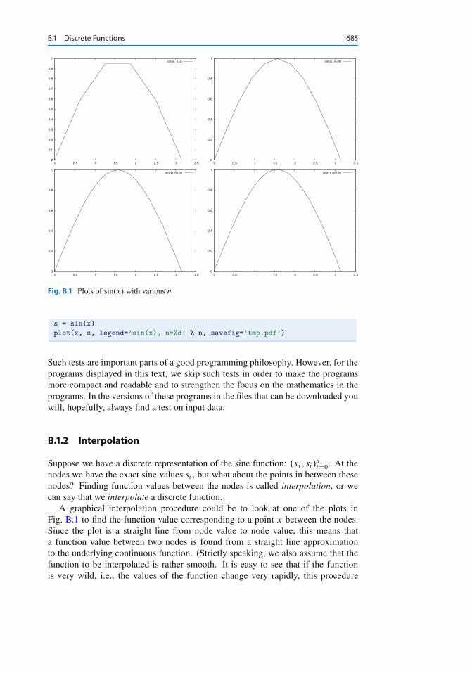
B.1 Discrete Functions 685
0
0.1
0.2
0.3
0.4
0.5
0.6
0.7
0.8
0.9
1
0 0.5 1 1.5 2 2.5 3 3.5
sin(x), n=5
0
0.2
0.4
0.6
0.8
1
0 0.5 1 1.5 2 2.5 3 3.5
sin(x), n=10
0
0.2
0.4
0.6
0.8
1
0 0.5 1 1.5 2 2.5 3 3.5
sin(x), n=20
0
0.2
0.4
0.6
0.8
1
0 0.5 1 1.5 2 2.5 3 3.5
sin(x), n=100
Fig. B.1 Plots of sin.x/ with various n
s = sin(x)
plot(x, s, legend=’sin(x), n=%d’ % n, savefig=’tmp.pdf’)
Such tests are important parts of a good programming philosophy. However, for theprograms displayed in this text, we skip such tests in order to make the programsmore compact and readable and to strengthen the focus on the mathematics in theprograms. In the versions of these programs in the files that can be downloaded youwill, hopefully, always find a test on input data.
B.1.2 Interpolation
Suppose we have a discrete representation of the sine function: .xi ; si /niD0. At the
nodes we have the exact sine values si , but what about the points in between thesenodes? Finding function values between the nodes is called interpolation, or wecan say that we interpolate a discrete function.
A graphical interpolation procedure could be to look at one of the plots inFig. B.1 to find the function value corresponding to a point x between the nodes.Since the plot is a straight line from node value to node value, this means thata function value between two nodes is found from a straight line approximationto the underlying continuous function. (Strictly speaking, we also assume that thefunction to be interpolated is rather smooth. It is easy to see that if the functionis very wild, i.e., the values of the function change very rapidly, this procedure
686 B Introduction to Discrete Calculus
may fail even for very large values of n. Section 5.4.2 provides an example.) Weformulate this procedure precisely in terms of mathematics in the next paragraph.
Assume that we know that a given x� lies in the interval from x D xk to xkC1,where the integer k is given. In the interval xk � x < xkC1, we define the linearfunction that passes through .xk; sk/ and .xkC1; skC1/:
Sk.x/ D sk C skC1 � sk
xkC1 � xk
.x � xk/ : (B.3)
That is, Sk.x/ coincides with sin.x/ at xk and xkC1, and between these nodes,Sk.x/ is linear. We say that Sk.x/ interpolates the discrete function .xi ; si /
niD0 on
the interval Œxk; xkC1�.
B.1.3 Evaluating the Approximation
Given the values .xi ; si /niD0 and the formula (B.3), we want to compute an approxi-
mation of the sine function for any x in the interval from x D 0 to x D � . In orderto do that, we have to compute k for a given value of x. More precisely, for a givenx we have to find k such that xk � x � xkC1. We can do that by defining
k D bx=hc
where the function bzc denotes the largest integer that is smaller than z. In Python,bzc is computed by int(z). The program below takes x and n as input and com-putes the approximation of sin.x/. The program prints the approximation S.x/ andthe exact value of sin.x/ so we can look at the development of the error when n isincreased. (The value is not really exact, it is the value of sin.x/ provided by thecomputer, math.sin(x), and this value is calculated from an algorithm that onlyyields an approximation to sin.x/. Exercise 3.37 provides an example of the typeof algorithm in question.)
from numpy import *
import sys
xp = eval(sys.argv[1])
n = int(sys.argv[2])
def S_k(k):
return s[k] + \
((s[k+1] - s[k])/(x[k+1] - x[k]))*(xp - x[k])
h = pi/n
x = linspace(0, pi, n+1)
s = sin(x)
k = int(xp/h)
print ’Approximation of sin(%s): ’ % xp, S_k(k)
print ’Exact value of sin(%s): ’ % xp, sin(xp)
print ’Eror in approximation: ’, sin(xp) - S_k(k)
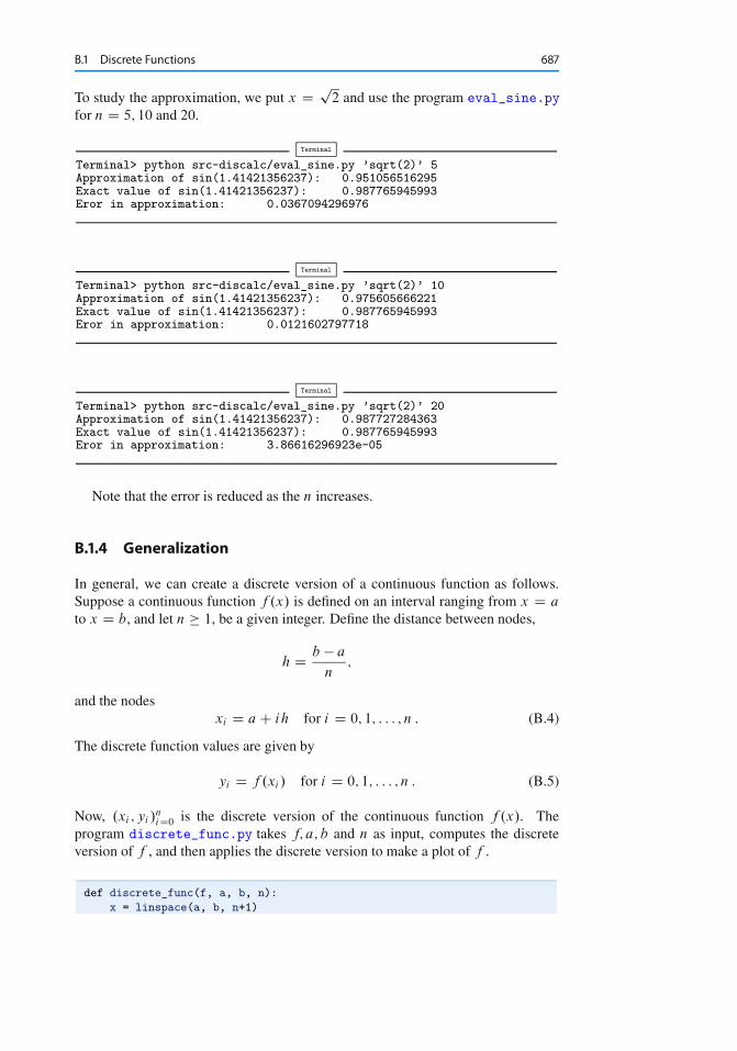
B.1 Discrete Functions 687
To study the approximation, we put x D p2 and use the program eval_sine.py
for n D 5; 10 and 20.
Terminal
Terminal> python src-discalc/eval_sine.py ’sqrt(2)’ 5Approximation of sin(1.41421356237): 0.951056516295Exact value of sin(1.41421356237): 0.987765945993Eror in approximation: 0.0367094296976
Terminal
Terminal> python src-discalc/eval_sine.py ’sqrt(2)’ 10Approximation of sin(1.41421356237): 0.975605666221Exact value of sin(1.41421356237): 0.987765945993Eror in approximation: 0.0121602797718
Terminal
Terminal> python src-discalc/eval_sine.py ’sqrt(2)’ 20Approximation of sin(1.41421356237): 0.987727284363Exact value of sin(1.41421356237): 0.987765945993Eror in approximation: 3.86616296923e-05
Note that the error is reduced as the n increases.
B.1.4 Generalization
In general, we can create a discrete version of a continuous function as follows.Suppose a continuous function f .x/ is defined on an interval ranging from x D a
to x D b, and let n � 1, be a given integer. Define the distance between nodes,
h D b � a
n;
and the nodesxi D a C ih for i D 0; 1; : : : ; n : (B.4)
The discrete function values are given by
yi D f .xi / for i D 0; 1; : : : ; n : (B.5)
Now, .xi ; yi /niD0 is the discrete version of the continuous function f .x/. The
program discrete_func.py takes f; a; b and n as input, computes the discreteversion of f , and then applies the discrete version to make a plot of f .
def discrete_func(f, a, b, n):
x = linspace(a, b, n+1)
688 B Introduction to Discrete Calculus
y = zeros(len(x))
for i in xrange(len(x)):
y[i] = func(x[i])
return x, y
from scitools.std import *
f_formula = sys.argv[1]
a = eval(sys.argv[2])
b = eval(sys.argv[3])
n = int(sys.argv[4])
f = StringFunction(f_formula)
x, y = discrete_func(f, a, b, n)
plot(x, y)
We can equally well make a vectorized version of the discrete_func function:
def discrete_func(f, a, b, n):
x = linspace(a, b, n+1)
y = f(x)
return x, y
However, for the StringFunction tool to work properly in vectorized mode, weneed to follow the recipe in Sect. 5.5.1:
f = StringFunction(f_formula)
f.vectorize(globals())
The corresponding vectorized program is found in the file discrete_func_vec.py.
B.2 Differentiation Becomes Finite Differences
You have heard about derivatives. Probably, the following formulas are well knownto you:
d
dxsin.x/ D cos.x/;
d
dxln.x/ D 1
x;
d
dxxm D mxm�1;
But why is differentiation so important? The reason is quite simple: the derivativeis a mathematical expression of change. And change is, of course, essential in mod-eling various phenomena. If we know the state of a system, and we know the lawsof change, then we can, in principle, compute the future of that system. Appendix Ctreats this topic in detail. Appendix A also computes the future of systems, basedon modeling changes, but without using differentiation. In Appendix C you will see
B.2 Differentiation Becomes Finite Differences 689
that reducing the step size in the difference equations results in derivatives insteadof pure differences. However, differentiation of continuous functions is somewhathard on a computer, so we often end up replacing the derivatives by differences.This idea is quite general, and every time we use a discrete representation of a func-tion, differentiation becomes differences, or finite differences as we usually say.
The mathematical definition of differentiation reads
f 0.x/ D lim"!0
f .x C "/ � f .x/
":
You have probably seen this definition many times, but have you understood whatit means and do you think the formula has a great practical value? Although thedefinition requires that we pass to the limit, we obtain quite good approximationsof the derivative by using a fixed positive value of ". More precisely, for a small" > 0, we have
f 0.x/ � f .x C "/ � f .x/
":
The fraction on the right-hand side is a finite difference approximation to the deriva-tive of f at the point x. Instead of using " it is more common to introduce h D " infinite differences, i.e., we like to write
f 0.x/ � f .x C h/ � f .x/
h: (B.6)
B.2.1 Differentiating the Sine Function
In order to get a feeling for how good the approximation (B.6) to the derivativereally is, we explore an example. Consider f .x/ D sin.x/ and the associatedderivative f 0.x/ D cos.x/. If we put x D 1;we have
f 0.1/ D cos.1/ � 0:540;
and by putting h D 1=100 in (B.6) we get
f 0.1/ � f .1 C 1=100/ � f .1/
1=100D sin.1:01/ � sin.1/
0:01� 0:536 :
The program forward_diff.py, shown below, computes the derivative of f .x/
using the approximation (B.6), where x and h are input parameters.
def diff(f, x, h):
return (f(x+h) - f(x))/float(h)
from math import *
import sys
x = eval(sys.argv[1])
h = eval(sys.argv[2])
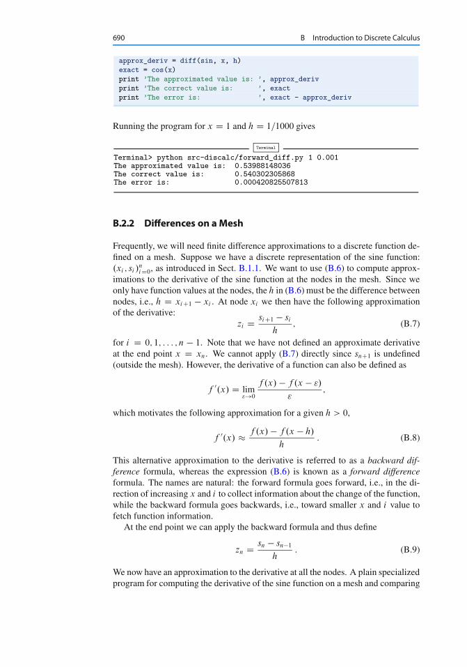
690 B Introduction to Discrete Calculus
approx_deriv = diff(sin, x, h)
exact = cos(x)
print ’The approximated value is: ’, approx_deriv
print ’The correct value is: ’, exact
print ’The error is: ’, exact - approx_deriv
Running the program for x D 1 and h D 1=1000 gives
Terminal
Terminal> python src-discalc/forward_diff.py 1 0.001The approximated value is: 0.53988148036The correct value is: 0.540302305868The error is: 0.000420825507813
B.2.2 Differences on aMesh
Frequently, we will need finite difference approximations to a discrete function de-fined on a mesh. Suppose we have a discrete representation of the sine function:.xi ; si /
niD0, as introduced in Sect. B.1.1. We want to use (B.6) to compute approx-
imations to the derivative of the sine function at the nodes in the mesh. Since weonly have function values at the nodes, the h in (B.6) must be the difference betweennodes, i.e., h D xiC1 � xi . At node xi we then have the following approximationof the derivative:
zi D siC1 � si
h; (B.7)
for i D 0; 1; : : : ; n � 1. Note that we have not defined an approximate derivativeat the end point x D xn. We cannot apply (B.7) directly since snC1 is undefined(outside the mesh). However, the derivative of a function can also be defined as
f 0.x/ D lim"!0
f .x/ � f .x � "/
";
which motivates the following approximation for a given h > 0,
f 0.x/ � f .x/ � f .x � h/
h: (B.8)
This alternative approximation to the derivative is referred to as a backward dif-ference formula, whereas the expression (B.6) is known as a forward differenceformula. The names are natural: the forward formula goes forward, i.e., in the di-rection of increasing x and i to collect information about the change of the function,while the backward formula goes backwards, i.e., toward smaller x and i value tofetch function information.
At the end point we can apply the backward formula and thus define
zn D sn � sn�1
h: (B.9)
We now have an approximation to the derivative at all the nodes. A plain specializedprogram for computing the derivative of the sine function on a mesh and comparing
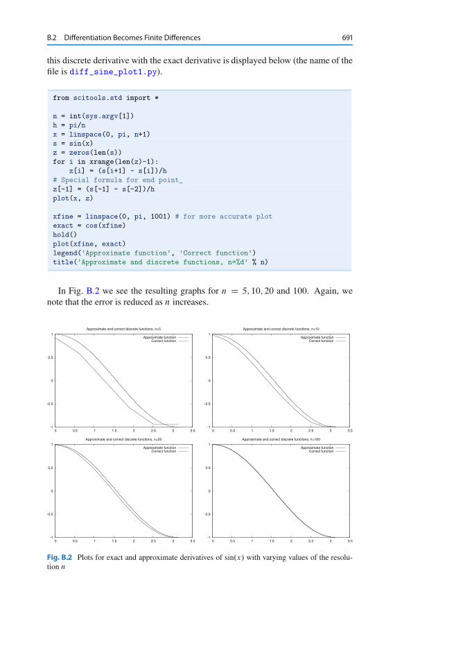
B.2 Differentiation Becomes Finite Differences 691
this discrete derivative with the exact derivative is displayed below (the name of thefile is diff_sine_plot1.py).
from scitools.std import *
n = int(sys.argv[1])
h = pi/n
x = linspace(0, pi, n+1)
s = sin(x)
z = zeros(len(s))
for i in xrange(len(z)-1):
z[i] = (s[i+1] - s[i])/h
# Special formula for end point_
z[-1] = (s[-1] - s[-2])/h
plot(x, z)
xfine = linspace(0, pi, 1001) # for more accurate plot
exact = cos(xfine)
hold()
plot(xfine, exact)
legend(’Approximate function’, ’Correct function’)
title(’Approximate and discrete functions, n=%d’ % n)
In Fig. B.2 we see the resulting graphs for n D 5; 10; 20 and 100. Again, wenote that the error is reduced as n increases.
-1
-0.5
0
0.5
1
0 0.5 1 1.5 2 2.5 3 3.5
Approximate and correct discrete functions, n=5
Approximate functionCorrect function
-1
-0.5
0
0.5
1
0 0.5 1 1.5 2 2.5 3 3.5
Approximate and correct discrete functions, n=10
Approximate functionCorrect function
-1
-0.5
0
0.5
1
0 0.5 1 1.5 2 2.5 3 3.5
Approximate and correct discrete functions, n=20
Approximate functionCorrect function
-1
-0.5
0
0.5
1
0 0.5 1 1.5 2 2.5 3 3.5
Approximate and correct discrete functions, n=100
Approximate functionCorrect function
Fig. B.2 Plots for exact and approximate derivatives of sin.x/ with varying values of the resolu-tion n
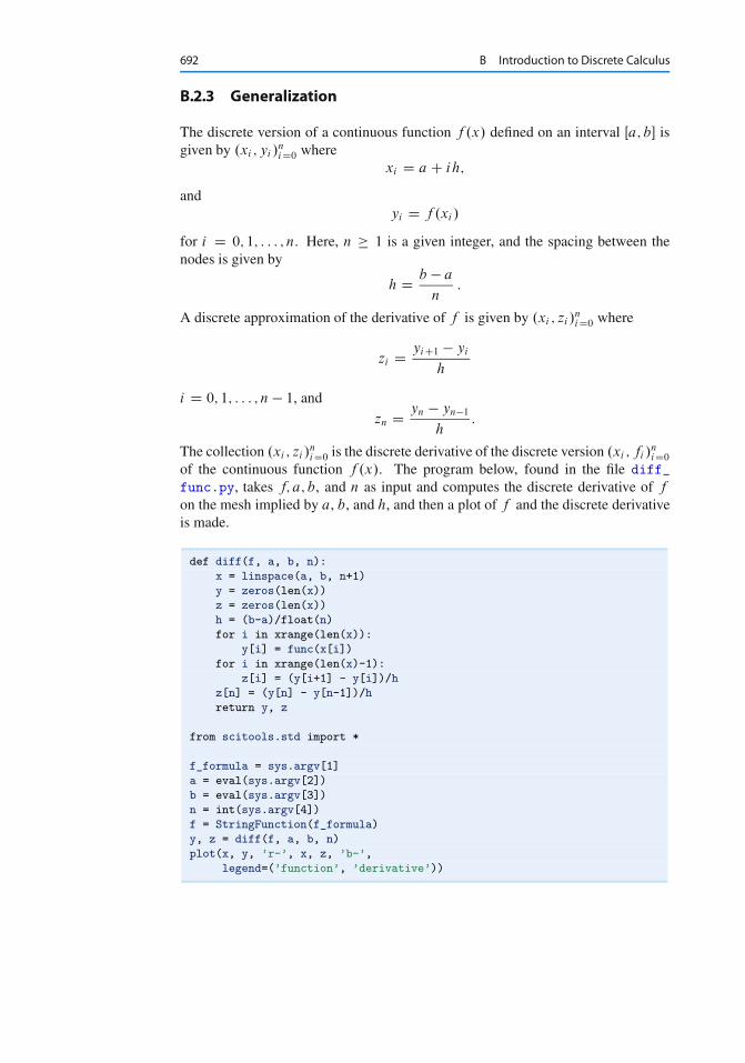
692 B Introduction to Discrete Calculus
B.2.3 Generalization
The discrete version of a continuous function f .x/ defined on an interval Œa; b� isgiven by .xi ; yi /
niD0 where
xi D a C ih;
andyi D f .xi /
for i D 0; 1; : : : ; n. Here, n � 1 is a given integer, and the spacing between thenodes is given by
h D b � a
n:
A discrete approximation of the derivative of f is given by .xi ; zi /niD0 where
zi D yiC1 � yi
h
i D 0; 1; : : : ; n � 1, and
zn D yn � yn�1
h:
The collection .xi ; zi /niD0 is the discrete derivative of the discrete version .xi ; fi /
niD0
of the continuous function f .x/. The program below, found in the file diff_func.py, takes f; a; b, and n as input and computes the discrete derivative of f
on the mesh implied by a, b, and h, and then a plot of f and the discrete derivativeis made.
def diff(f, a, b, n):
x = linspace(a, b, n+1)
y = zeros(len(x))
z = zeros(len(x))
h = (b-a)/float(n)
for i in xrange(len(x)):
y[i] = func(x[i])
for i in xrange(len(x)-1):
z[i] = (y[i+1] - y[i])/h
z[n] = (y[n] - y[n-1])/h
return y, z
from scitools.std import *
f_formula = sys.argv[1]
a = eval(sys.argv[2])
b = eval(sys.argv[3])
n = int(sys.argv[4])
f = StringFunction(f_formula)
y, z = diff(f, a, b, n)
plot(x, y, ’r-’, x, z, ’b-’,
legend=(’function’, ’derivative’))
B.3 Integration Becomes Summation 693
B.3 Integration Becomes Summation
Some functions can be integrated analytically. You may remember the followingcases,
Zxmdx D 1
m C 1xmC1 for m ¤ �1;
Zsin.x/dx D � cos.x/;
Zx
1 C x2dx D 1
2ln�x2 C 1
�:
These are examples of so-called indefinite integrals. If the function can be inte-grated analytically, it is straightforward to evaluate an associated definite integral.Recall, in general, that
Œf .x/�ba D f .b/ � f .a/:
Some particular examples are
1Z
0
xmdx D�
1
m C 1xmC1
1
0
D 1
m C 1;
�Z
0
sin.x/dx D Œ� cos.x/��0 D 2;
1Z
0
x
1 C x2dx D
�1
2ln�x2 C 1
�1
0
D 1
2ln 2:
But lots of functions cannot be integrated analytically and therefore definite inte-grals must be computed using some sort of numerical approximation. Above, weintroduced the discrete version of a function, and we will now use this constructionto compute an approximation of a definite integral.
B.3.1 Dividing into Subintervals
Let us start by considering the problem of computing the integral of sin.x/ fromx D 0 to x D � . This is not the most exciting or challenging mathematical prob-lem you can think of, but it is good practice to start with a problem you know wellwhen you want to learn a new method. In Sect. B.1.1 we introduce a discrete func-tion .xi ; si /
niD0 where h D �=n; si D sin.xi / and xi D ih for i D 0; 1; : : : ; n.
Furthermore, in the interval xk � x < xkC1, we defined the linear function
Sk.x/ D sk C skC1 � sk
xkC1 � xk
.x � xk/:
694 B Introduction to Discrete Calculus
We want to compute an approximation of the integral of the function sin.x/ fromx D 0 to x D � . The integral
�Z
0
sin.x/dx
can be divided into subintegrals defined on the intervals xk � x < xkC1, leading tothe following sum of integrals:
�Z
0
sin.x/dx Dn�1XkD0
xkC1Z
xk
sin.x/dx :
To get a feeling for this split of the integral, let us spell the sum out in the case ofonly four subintervals. Then n D 4; h D �=4,
x0 D 0;
x1 D �=4;
x2 D �=2;
x3 D 3�=4
x4 D �:
The interval from 0 to � is divided into four intervals of equal length, and we candivide the integral similarly,
�Z
0
sin.x/dx Dx1Z
x0
sin.x/dx Cx2Z
x1
sin.x/dxC
x3Z
x2
sin.x/dx Cx4Z
x3
sin.x/dx : (B.10)
So far we have changed nothing – the integral can be split in this way - with no ap-proximation at all. But we have reduced the problem of approximating the integral
�Z
0
sin.x/dx
down to approximating integrals on the subintervals, i.e. we need approximationsof all the following integrals
x1Z
x0
sin.x/dx;
x2Z
x1
sin.x/dx;
x3Z
x2
sin.x/dx;
x4Z
x3
sin.x/dx :
The idea is that the function to be integrated changes less over the subintervals thanover the whole domain Œ0; �� and it might be reasonable to approximate the sine bya straight line, Sk.x/, over each subinterval. The integration over a subinterval willthen be very easy.
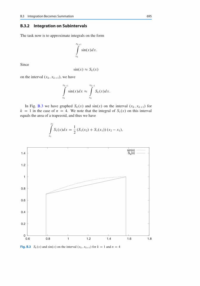
B.3 Integration Becomes Summation 695
B.3.2 Integration on Subintervals
The task now is to approximate integrals on the form
xkC1Z
xk
sin.x/dx:
Sincesin.x/ � Sk.x/
on the interval .xk; xkC1/, we have
xkC1Z
xk
sin.x/dx �xkC1Z
xk
Sk.x/dx:
In Fig. B.3 we have graphed Sk.x/ and sin.x/ on the interval .xk; xkC1/ fork D 1 in the case of n D 4. We note that the integral of S1.x/ on this intervalequals the area of a trapezoid, and thus we have
x2Z
x1
S1.x/dx D 1
2.S1.x2/ C S1.x1// .x2 � x1/;
0
0.2
0.4
0.6
0.8
1
1.2
1.4
0.6 0.8 1 1.2 1.4 1.6 1.8
sin(x)Sk(x)
Fig. B.3 Sk.x/ and sin.x/ on the interval .xk ; xkC1/ for k D 1 and n D 4
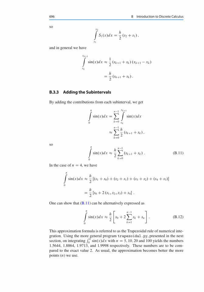
696 B Introduction to Discrete Calculus
sox2Z
x1
S1.x/dx D h
2.s2 C s1/ ;
and in general we have
xkC1Z
xk
sin.x/dx � 1
2.skC1 C sk/ .xkC1 � xk/
D h
2.skC1 C sk/ :
B.3.3 Adding the Subintervals
By adding the contributions from each subinterval, we get
�Z
0
sin.x/dx Dn�1XkD0
xkC1Z
xk
sin.x/dx
�n�1XkD0
h
2.skC1 C sk/ ;
so�Z
0
sin.x/dx � h
2
n�1XkD0
.skC1 C sk/ : (B.11)
In the case of n D 4, we have
�Z
0
sin.x/dx � h
2Œ.s1 C s0/ C .s2 C s1/ C .s3 C s2/ C .s4 C s3/�
D h
2Œs0 C 2 .s1Cs2Cs3/ C s4� :
One can show that (B.11) can be alternatively expressed as
�Z
0
sin.x/dx � h
2
"s0 C 2
n�1XkD1
sk C sn
#: (B.12)
This approximation formula is referred to as the Trapezoidal rule of numerical inte-gration. Using the more general program trapezoidal.py, presented in the nextsection, on integrating
R �
0sin.x/dx with n D 5; 10; 20 and 100 yields the numbers
1.5644, 1.8864, 1.9713, and 1.9998 respectively. These numbers are to be com-pared to the exact value 2. As usual, the approximation becomes better the morepoints (n) we use.
B.3 Integration Becomes Summation 697
B.3.4 Generalization
An approximation of the integral
bZ
a
f .x/dx
can be computed using the discrete version of a continuous function f .x/ definedon an interval Œa; b�. We recall that the discrete version of f is given by .xi ; yi /
niD0
wherexi D a C ih; and yi D f .xi /
for i D 0; 1; : : : ; n. Here, n � 1 is a given integer and h D .b � a/=n. TheTrapezoidal rule can now be written as
bZ
a
f .x/dx � h
2
"y0 C 2
n�1XkD1
yk C yn
#:
The program trapezoidal.py implements the Trapezoidal rule for a generalfunction f .
def trapezoidal(f, a, b, n):
h = (b-a)/float(n)
I = f(a) + f(b)
for k in xrange(1, n, 1):
x = a + k*h
I += 2*f(x)
I *= h/2
return I
from math import *
from scitools.StringFunction import StringFunction
import sys
def test(argv=sys.argv):
f_formula = argv[1]
a = eval(argv[2])
b = eval(argv[3])
n = int(argv[4])
f = StringFunction(f_formula)
I = trapezoidal(f, a, b, n)
print ’Approximation of the integral: ’, I
if __name__ == ’__main__’:
test()
We have made the file as a module such that you can easily import thetrapezoidal function in another program. Let us do that: we make a table
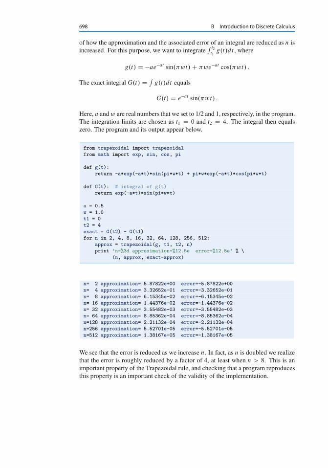
698 B Introduction to Discrete Calculus
of how the approximation and the associated error of an integral are reduced as n isincreased. For this purpose, we want to integrate
R t2t1
g.t/dt , where
g.t/ D �ae�at sin.�wt/ C �we�at cos.�wt/ :
The exact integral G.t/ D Rg.t/dt equals
G.t/ D e�at sin.�wt/ :
Here, a andw are real numbers that we set to 1/2 and 1, respectively, in the program.The integration limits are chosen as t1 D 0 and t2 D 4. The integral then equalszero. The program and its output appear below.
from trapezoidal import trapezoidal
from math import exp, sin, cos, pi
def g(t):
return -a*exp(-a*t)*sin(pi*w*t) + pi*w*exp(-a*t)*cos(pi*w*t)
def G(t): # integral of g(t)
return exp(-a*t)*sin(pi*w*t)
a = 0.5
w = 1.0
t1 = 0
t2 = 4
exact = G(t2) - G(t1)
for n in 2, 4, 8, 16, 32, 64, 128, 256, 512:
approx = trapezoidal(g, t1, t2, n)
print ’n=%3d approximation=%12.5e error=%12.5e’ % \
(n, approx, exact-approx)
n= 2 approximation= 5.87822e+00 error=-5.87822e+00
n= 4 approximation= 3.32652e-01 error=-3.32652e-01
n= 8 approximation= 6.15345e-02 error=-6.15345e-02
n= 16 approximation= 1.44376e-02 error=-1.44376e-02
n= 32 approximation= 3.55482e-03 error=-3.55482e-03
n= 64 approximation= 8.85362e-04 error=-8.85362e-04
n=128 approximation= 2.21132e-04 error=-2.21132e-04
n=256 approximation= 5.52701e-05 error=-5.52701e-05
n=512 approximation= 1.38167e-05 error=-1.38167e-05
We see that the error is reduced as we increase n. In fact, as n is doubled we realizethat the error is roughly reduced by a factor of 4, at least when n > 8. This is animportant property of the Trapezoidal rule, and checking that a program reproducesthis property is an important check of the validity of the implementation.
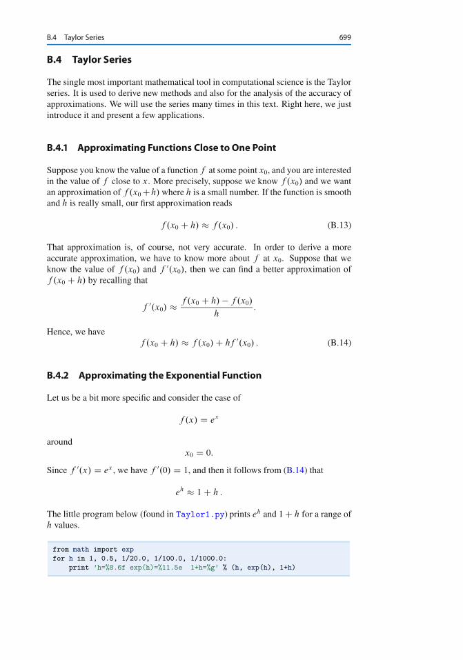
B.4 Taylor Series 699
B.4 Taylor Series
The single most important mathematical tool in computational science is the Taylorseries. It is used to derive new methods and also for the analysis of the accuracy ofapproximations. We will use the series many times in this text. Right here, we justintroduce it and present a few applications.
B.4.1 Approximating Functions Close to One Point
Suppose you know the value of a function f at some point x0, and you are interestedin the value of f close to x. More precisely, suppose we know f .x0/ and we wantan approximation of f .x0 Ch/ where h is a small number. If the function is smoothand h is really small, our first approximation reads
f .x0 C h/ � f .x0/ : (B.13)
That approximation is, of course, not very accurate. In order to derive a moreaccurate approximation, we have to know more about f at x0. Suppose that weknow the value of f .x0/ and f 0.x0/, then we can find a better approximation off .x0 C h/ by recalling that
f 0.x0/ � f .x0 C h/ � f .x0/
h:
Hence, we havef .x0 C h/ � f .x0/ C hf 0.x0/ : (B.14)
B.4.2 Approximating the Exponential Function
Let us be a bit more specific and consider the case of
f .x/ D ex
aroundx0 D 0:
Since f 0.x/ D ex , we have f 0.0/ D 1, and then it follows from (B.14) that
eh � 1 C h :
The little program below (found in Taylor1.py) prints eh and 1 C h for a range ofh values.
from math import exp
for h in 1, 0.5, 1/20.0, 1/100.0, 1/1000.0:
print ’h=%8.6f exp(h)=%11.5e 1+h=%g’ % (h, exp(h), 1+h)
700 B Introduction to Discrete Calculus
h=1.000000 exp(h)=2.71828e+00 1+h=2
h=0.500000 exp(h)=1.64872e+00 1+h=1.5
h=0.050000 exp(h)=1.05127e+00 1+h=1.05
h=0.010000 exp(h)=1.01005e+00 1+h=1.01
h=0.001000 exp(h)=1.00100e+00 1+h=1.001
As expected, 1 C h is a good approximation to eh the smaller h is.
B.4.3 More Accurate Expansions
The approximations given by (B.13) and (B.14) are referred to as Taylor series. Youcan read much more about Taylor series in any Calculus book. More specifically,(B.13) and (B.14) are known as the zeroth- and first-order Taylor series, respec-tively. The second-order Taylor series is given by
f .x0 C h/ � f .x0/ C hf 0.x0/ C h2
2f 00.x0/; (B.15)
the third-order series is given by
f .x0 C h/ � f .x0/ C hf 0.x0/ C h2
2f 00.x0/ C h3
6f 000.x0/; (B.16)
and the fourth-order series reads
f .x0 C h/ � f .x0/ C hf 0.x0/ C h2
2f 00.x0/ C h3
6f 000.x0/ C h4
24f 0000.x0/: (B.17)
In general, the n-th order Taylor series is given by
f .x0 C h/ �nX
kD0
hk
kŠf .k/.x0/; (B.18)
where we recall that f .k/ denotes the k�th derivative of f , and
kŠ D 1 � 2 � 3 � 4 � � � .k � 1/ � k
is the factorial. By again considering f .x/ D ex and x0 D 0, we have
f .x0/ D f 0.x0/ D f 00.x0/ D f 000.x0/ D f 0000.x0/ D 1
which gives the following Taylor series:
eh � 1 C h C 1
2h2 C 1
6h3 C 1
24h4 :
The program below, called Taylor2.py, prints the error of these approximationsfor a given value of h (note that we can easily build up a Taylor series in a list byadding a new term to the last computed term in the list).
B.4 Taylor Series 701
from math import exp
import sys
h = float(sys.argv[1])
Taylor_series = []
Taylor_series.append(1)
Taylor_series.append(Taylor_series[-1] + h)
Taylor_series.append(Taylor_series[-1] + (1/2.0)*h**2)
Taylor_series.append(Taylor_series[-1] + (1/6.0)*h**3)
Taylor_series.append(Taylor_series[-1] + (1/24.0)*h**4)
print ’h =’, h
for order in range(len(Taylor_series)):
print ’order=%d, error=%g’ % \
(order, exp(h) - Taylor_series[order])
By running the program with h D 0:2, we have the following output:
h = 0.2
order=0, error=0.221403
order=1, error=0.0214028
order=2, error=0.00140276
order=3, error=6.94248e-05
order=4, error=2.75816e-06
We see how much the approximation is improved by adding more terms. For h D 3
all these approximations are useless:
h = 3.0
order=0, error=19.0855
order=1, error=16.0855
order=2, error=11.5855
order=3, error=7.08554
order=4, error=3.71054
However, by adding more terms we can get accurate results for any h. The methodfrom Sect. A.1.8 computes the Taylor series for ex with n terms in general. Runningthe associated program exp_Taylor_series_diffeq.py for various values of h
shows how much is gained by adding more terms to the Taylor series. For h D 3,e3 D 20:086 and we have
n C 1 Taylor series2 44 138 19.84616 20.086
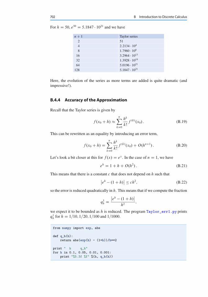
702 B Introduction to Discrete Calculus
For h D 50, e50 D 5:1847 � 1021 and we have
n C 1 Taylor series2 514 2:2134 � 104
8 1:7960 � 108
16 3:2964 � 1013
32 1:3928 � 1019
64 5:0196 � 1021
128 5:1847 � 1021
Here, the evolution of the series as more terms are added is quite dramatic (andimpressive!).
B.4.4 Accuracy of the Approximation
Recall that the Taylor series is given by
f .x0 C h/ �nX
kD0
hk
kŠf .k/.x0/ : (B.19)
This can be rewritten as an equality by introducing an error term,
f .x0 C h/ DnX
kD0
hk
kŠf .k/.x0/ C O.hnC1/ : (B.20)
Let’s look a bit closer at this for f .x/ D ex . In the case of n D 1, we have
eh D 1 C h C O.h2/ : (B.21)
This means that there is a constant c that does not depend on h such thatˇ̌eh � .1 C h/
ˇ̌ � ch2; (B.22)
so the error is reduced quadratically in h. This means that if we compute the fraction
q1h D
ˇ̌eh � .1 C h/
ˇ̌
h2;
we expect it to be bounded as h is reduced. The program Taylor_err1.py printsq1
h for h D 1=10; 1=20; 1=100 and 1=1000.
from numpy import exp, abs
def q_h(h):
return abs(exp(h) - (1+h))/h**2
print " h q_h"
for h in 0.1, 0.05, 0.01, 0.001:
print "%5.3f %f" %(h, q_h(h))
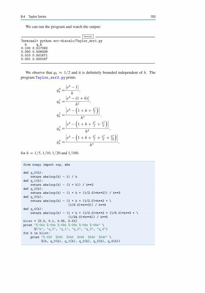
B.4 Taylor Series 703
We can run the program and watch the output:
Terminal
Terminal> python src-discalc/Taylor_err1.pyh q_h
0.100 0.5170920.050 0.5084390.010 0.5016710.001 0.500167
We observe that qh � 1=2 and it is definitely bounded independent of h. Theprogram Taylor_err2.py prints
q0h D
ˇ̌eh � 1
ˇ̌
h;
q1h D
ˇ̌eh � .1 C h/
ˇ̌
h2;
q2h D
ˇ̌ˇeh �
�1 C h C h2
2
�ˇ̌ˇ
h3;
q3h D
ˇ̌ˇeh �
�1 C h C h2
2C h3
6
�ˇ̌ˇ
h4;
q4h D
ˇ̌ˇeh �
�1 C h C h2
2C h3
6C h4
24
�ˇ̌ˇ
h5;
for h D 1=5; 1=10; 1=20 and 1=100.
from numpy import exp, abs
def q_0(h):
return abs(exp(h) - 1) / h
def q_1(h):
return abs(exp(h) - (1 + h)) / h**2
def q_2(h):
return abs(exp(h) - (1 + h + (1/2.0)*h**2)) / h**3
def q_3(h):
return abs(exp(h) - (1 + h + (1/2.0)*h**2 + \
(1/6.0)*h**3)) / h**4
def q_4(h):
return abs(exp(h) - (1 + h + (1/2.0)*h**2 + (1/6.0)*h**3 + \
(1/24.0)*h**4)) / h**5
hlist = [0.2, 0.1, 0.05, 0.01]
print "%-05s %-09s %-09s %-09s %-09s %-09s" \
%("h", "q_0", "q_1", "q_2", "q_3", "q_4")
for h in hlist:
print "%.02f %04f %04f %04f %04f %04f" \
%(h, q_0(h), q_1(h), q_2(h), q_3(h), q_4(h))
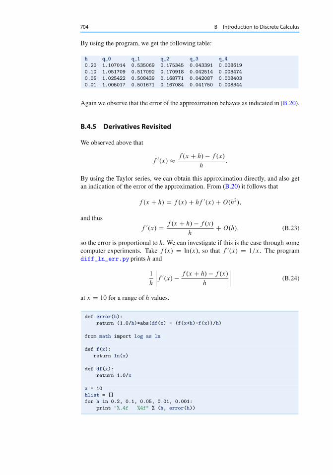
704 B Introduction to Discrete Calculus
By using the program, we get the following table:
h q_0 q_1 q_2 q_3 q_4
0.20 1.107014 0.535069 0.175345 0.043391 0.008619
0.10 1.051709 0.517092 0.170918 0.042514 0.008474
0.05 1.025422 0.508439 0.168771 0.042087 0.008403
0.01 1.005017 0.501671 0.167084 0.041750 0.008344
Again we observe that the error of the approximation behaves as indicated in (B.20).
B.4.5 Derivatives Revisited
We observed above that
f 0.x/ � f .x C h/ � f .x/
h:
By using the Taylor series, we can obtain this approximation directly, and also getan indication of the error of the approximation. From (B.20) it follows that
f .x C h/ D f .x/ C hf 0.x/ C O.h2/;
and thus
f 0.x/ D f .x C h/ � f .x/
hC O.h/; (B.23)
so the error is proportional to h. We can investigate if this is the case through somecomputer experiments. Take f .x/ D ln.x/, so that f 0.x/ D 1=x. The programdiff_ln_err.py prints h and
1
h
ˇ̌ˇ̌f 0.x/ � f .x C h/ � f .x/
h
ˇ̌ˇ̌ (B.24)
at x D 10 for a range of h values.
def error(h):
return (1.0/h)*abs(df(x) - (f(x+h)-f(x))/h)
from math import log as ln
def f(x):
return ln(x)
def df(x):
return 1.0/x
x = 10
hlist = []
for h in 0.2, 0.1, 0.05, 0.01, 0.001:
print "%.4f %4f" % (h, error(h))
B.4 Taylor Series 705
From the output
0.2000 0.004934
0.1000 0.004967
0.0500 0.004983
0.0100 0.004997
0.0010 0.005000
we observe that the quantity in (B.24) is constant (� 0:5) independent of h, whichindicates that the error is proportional to h.
B.4.6 More Accurate Difference Approximations
We can also use the Taylor series to derive more accurate approximations of thederivatives. From (B.20), we have
f .x C h/ � f .x/ C hf 0.x/ C h2
2f 00.x/ C O.h3/ : (B.25)
By using �h instead of h, we get
f .x � h/ � f .x/ � hf 0.x/ C h2
2f 00.x/ C O.h3/ : (B.26)
By subtracting (B.26) from (B.25), we have
f .x C h/ � f .x � h/ D 2hf 0.x/ C O.h3/;
and consequently
f 0.x/ D f .x C h/ � f .x � h/
2hC O.h2/: (B.27)
Note that the error is now O.h2/ whereas the error term of (B.23) is O.h/. In orderto see if the error is actually reduced, let us compare the following two approxima-tions
f 0.x/ � f .x C h/ � f .x/
hand f 0.x/ � f .x C h/ � f .x � h/
2h
by applying them to the discrete version of sin.x/ on the interval .0; �/. As usual,we let n � 1 be a given integer, and define the mesh
xi D ih for i D 0; 1; : : : ; n;
where h D �=n. At the nodes, we have the functional values
si D sin.xi / for i D 0; 1; : : : ; n;
706 B Introduction to Discrete Calculus
and at the inner nodes we define the first (F) and second (S) order approximationsof the derivatives given by
d Fi D siC1 � si
h;
andd S
i D siC1 � si�1
2h;
respectively for i D 1; 2; : : : ; n � 1. These values should be compared to the exactderivative given by
di D cos.xi / for i D 1; 2; : : : ; n � 1:
The following program, found in diff_1st2nd_order.py, plots the discrete func-tions .xi ; di /
n�1iD1; .xi ; d F
i /n�1iD1; and .xi ; d S
i /n�1iD1 for a given n. Note that the first three
functions in this program are completely general in that they can be used for anyf .x/ on any mesh. The special case of f .x/ D sin.x/ and comparing first- andsecond-order formulas is implemented in the example function. This latter func-tion is called in the test block of the file. That is, the file is a module and we canreuse the first three functions in other programs (in particular, we can use the thirdfunction in the next example).
def first_order(f, x, h):
return (f(x+h) - f(x))/h
def second_order(f, x, h):
return (f(x+h) - f(x-h))/(2*h)
def derivative_on_mesh(formula, f, a, b, n):
"""
Differentiate f(x) at all internal points in a mesh
on [a,b] with n+1 equally spaced points.
The differentiation formula is given by formula(f, x, h).
"""
h = (b-a)/float(n)
x = linspace(a, b, n+1)
df = zeros(len(x))
for i in xrange(1, len(x)-1):
df[i] = formula(f, x[i], h)
# Return x and values at internal points only
return x[1:-1], df[1:-1]
def example(n):
a = 0; b = pi;
x, dF = derivative_on_mesh(first_order, sin, a, b, n)
x, dS = derivative_on_mesh(second_order, sin, a, b, n)
# Accurate plot of the exact derivative at internal points
h = (b-a)/float(n)
xfine = linspace(a+h, b-h, 1001)
exact = cos(xfine)
plot(x, dF, ’r-’, x, dS, ’b-’, xfine, exact, ’y-’,
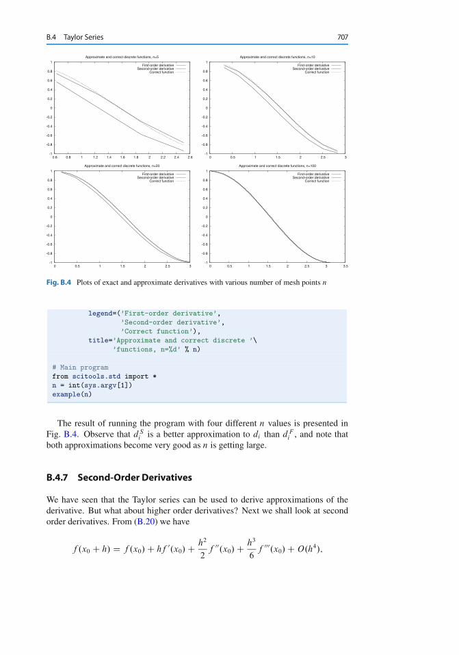
B.4 Taylor Series 707
-1
-0.8
-0.6
-0.4
-0.2
0
0.2
0.4
0.6
0.8
1
0.6 0.8 1 1.2 1.4 1.6 1.8 2 2.2 2.4 2.6
Approximate and correct discrete functions, n=5
First-order derivativeSecond-order derivative
Correct function
-1
-0.8
-0.6
-0.4
-0.2
0
0.2
0.4
0.6
0.8
1
0 0.5 1 1.5 2 2.5 3
Approximate and correct discrete functions, n=10
First-order derivativeSecond-order derivative
Correct function
-1
-0.8
-0.6
-0.4
-0.2
0
0.2
0.4
0.6
0.8
1
0 0.5 1 1.5 2 2.5 3
Approximate and correct discrete functions, n=20
First-order derivativeSecond-order derivative
Correct function
-1
-0.8
-0.6
-0.4
-0.2
0
0.2
0.4
0.6
0.8
1
0 0.5 1 1.5 2 2.5 3 3.5
Approximate and correct discrete functions, n=100
First-order derivativeSecond-order derivative
Correct function
Fig. B.4 Plots of exact and approximate derivatives with various number of mesh points n
legend=(’First-order derivative’,
’Second-order derivative’,
’Correct function’),
title=’Approximate and correct discrete ’\
’functions, n=%d’ % n)
# Main program
from scitools.std import *
n = int(sys.argv[1])
example(n)
The result of running the program with four different n values is presented inFig. B.4. Observe that d S
i is a better approximation to di than d Fi , and note that
both approximations become very good as n is getting large.
B.4.7 Second-Order Derivatives
We have seen that the Taylor series can be used to derive approximations of thederivative. But what about higher order derivatives? Next we shall look at secondorder derivatives. From (B.20) we have
f .x0 C h/ D f .x0/ C hf 0.x0/ C h2
2f 00.x0/ C h3
6f 000.x0/ C O.h4/;
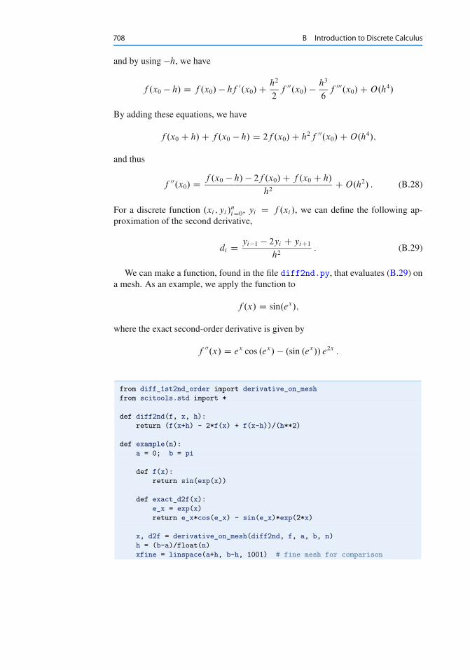
708 B Introduction to Discrete Calculus
and by using �h, we have
f .x0 � h/ D f .x0/ � hf 0.x0/ C h2
2f 00.x0/ � h3
6f 000.x0/ C O.h4/
By adding these equations, we have
f .x0 C h/ C f .x0 � h/ D 2f .x0/ C h2f 00.x0/ C O.h4/;
and thus
f 00.x0/ D f .x0 � h/ � 2f .x0/ C f .x0 C h/
h2C O.h2/ : (B.28)
For a discrete function .xi ; yi /niD0, yi D f .xi /, we can define the following ap-
proximation of the second derivative,
di D yi�1 � 2yi C yiC1
h2: (B.29)
We can make a function, found in the file diff2nd.py, that evaluates (B.29) ona mesh. As an example, we apply the function to
f .x/ D sin.ex/;
where the exact second-order derivative is given by
f 00.x/ D ex cos .ex/ � .sin .ex// e2x :
from diff_1st2nd_order import derivative_on_mesh
from scitools.std import *
def diff2nd(f, x, h):
return (f(x+h) - 2*f(x) + f(x-h))/(h**2)
def example(n):
a = 0; b = pi
def f(x):
return sin(exp(x))
def exact_d2f(x):
e_x = exp(x)
return e_x*cos(e_x) - sin(e_x)*exp(2*x)
x, d2f = derivative_on_mesh(diff2nd, f, a, b, n)
h = (b-a)/float(n)
xfine = linspace(a+h, b-h, 1001) # fine mesh for comparison
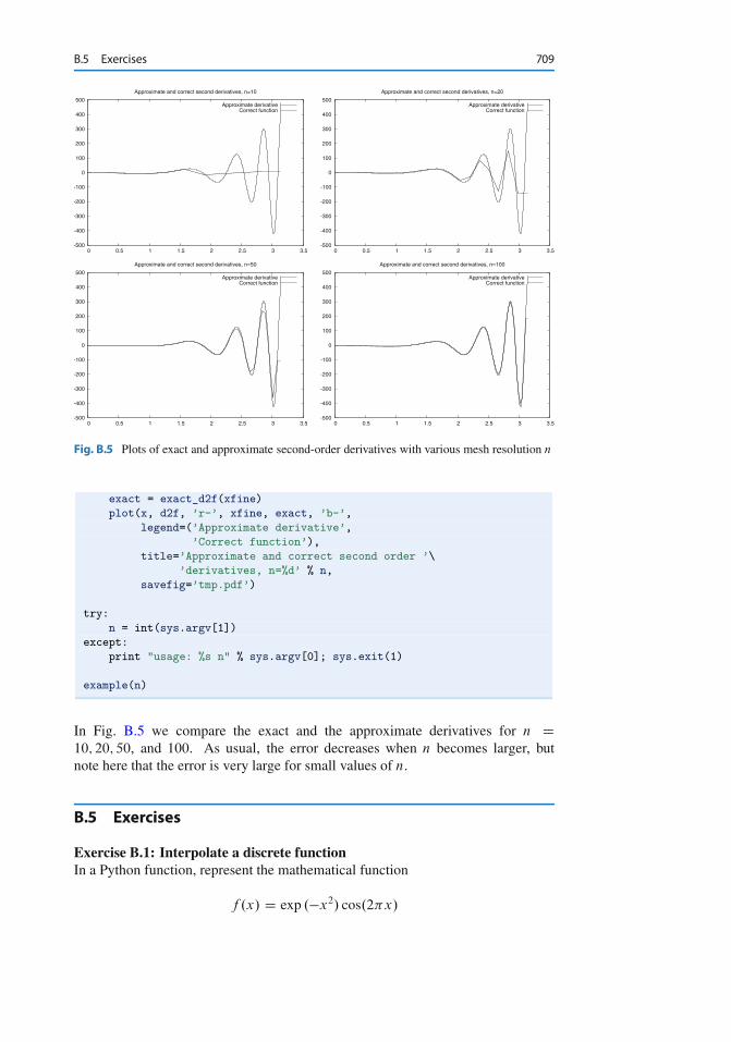
B.5 Exercises 709
-500
-400
-300
-200
-100
0
100
200
300
400
500
0 0.5 1 1.5 2 2.5 3 3.5
Approximate and correct second derivatives, n=10
Approximate derivativeCorrect function
-500
-400
-300
-200
-100
0
100
200
300
400
500
0 0.5 1 1.5 2 2.5 3 3.5
Approximate and correct second derivatives, n=20
Approximate derivativeCorrect function
-500
-400
-300
-200
-100
0
100
200
300
400
500
0 0.5 1 1.5 2 2.5 3 3.5
Approximate and correct second derivatives, n=50
Approximate derivativeCorrect function
-500
-400
-300
-200
-100
0
100
200
300
400
500
0 0.5 1 1.5 2 2.5 3 3.5
Approximate and correct second derivatives, n=100
Approximate derivativeCorrect function
Fig. B.5 Plots of exact and approximate second-order derivatives with various mesh resolution n
exact = exact_d2f(xfine)
plot(x, d2f, ’r-’, xfine, exact, ’b-’,
legend=(’Approximate derivative’,
’Correct function’),
title=’Approximate and correct second order ’\
’derivatives, n=%d’ % n,
savefig=’tmp.pdf’)
try:
n = int(sys.argv[1])
except:
print "usage: %s n" % sys.argv[0]; sys.exit(1)
example(n)
In Fig. B.5 we compare the exact and the approximate derivatives for n D10; 20; 50, and 100. As usual, the error decreases when n becomes larger, butnote here that the error is very large for small values of n.
B.5 Exercises
Exercise B.1: Interpolate a discrete functionIn a Python function, represent the mathematical function
f .x/ D exp .�x2/ cos.2�x/
710 B Introduction to Discrete Calculus
on a mesh consisting of q C 1 equally spaced points on Œ�1; 1�, and return 1) theinterpolated function value at x D �0:45 and 2) the error in the interpolated value.Call the function and write out the error for q D 2; 4; 8; 16.Filename: interpolate_exp_cos.
Exercise B.2: Study a function for different parameter valuesDevelop a program that creates a plot of the function f .x/ D sin. 1
xC"/ for x in the
unit interval, where " > 0 is a given input parameter. Use n C 1 nodes in the plot.
a) Test the program using n D 10 and " D 1=5.b) Refine the program such that it plots the function for two values of n; say n and
n C 10.c) How large do you have to choose n in order for the difference between these
two functions to be less than 0:1?
Hint Each function gives an array. Create a while loop and use the max functionof the arrays to retrieve the maximum value and compare these.
d) Let " D 1=10 and recalculate.e) Let " D 1=20 and recalculate.f) Try to find a formula for how large n needs to be for a given value of " such that
increasing n further does not change the plot so much that it is visible on thescreen. Note that there is no exact answer to this question.
Filename: plot_sin_eps.
Exercise B.3: Study a function and its derivativeConsider the function
f .x/ D sin�
1
x C "
�
for x ranging from 0 to 1, and the derivative
f 0.x/ D � cos�
1xC"
�
.x C "/2:
Here, " is a given input parameter.
a) Develop a program that creates a plot of the derivative of f D f .x/ based ona finite difference approximation using n computational nodes. The programshould also graph the exact derivative given by f 0 D f 0.x/ above.
b) Test the program using n D 10 and " D 1=5.c) How large do you have to choose n in order for the difference between these
two functions to be less than 0:1?
Hint Each function gives an array. Create a while loop and use the max functionof the arrays to retrieve the maximum value and compare these.
d) Let " D 1=10 and recalculate.
B.5 Exercises 711
e) Let " D 1=20 and recalculate.f) Try to determine experimentally how large n needs to be for a given value of
" such that increasing n further does not change the plot so much that you canview it on the screen. Note, again, that there is no exact solution to this problem.
Filename: sin_deriv.
Exercise B.4: Use the Trapezoidal methodThe purpose of this exercise is to test the program trapezoidal.py.
a) Let
a D1Z
0
e4xdx D 1
4e4 � 1
4:
Compute the integral using the program trapezoidal.py and, for a given n,let a.n/ denote the result. Try to find, experimentally, how large you have tochoose n in order for
ja � a.n/j � "
where " D 1=100.b) Recalculate with " D 1=1000.c) Recalculate with " D 1=10;000.d) Try to figure out, in general, how large n has to be such that
ja � a.n/j � "
for a given value of ".
Filename: trapezoidal_test_exp.
Exercise B.5: Compute a sequence of integrals
a) Let
bk D1Z
0
xkdx D 1
k C 1;
and let bk.n/ denote the result of using the program trapezoidal.py to com-pute
R 1
0xkdx. For k D 4; 6 and 8, try to figure out, by doing numerical
experiments, how large n needs to be in order for bk.n/ to satisfy
ˇ̌ˇbk � bk.n/
ˇ̌ˇ � 0:0001:
Note that n will depend on k.
Hint Run the program for each k, look at the output, and calculateˇ̌ˇbk � bk.n/
ˇ̌ˇ
manually.
712 B Introduction to Discrete Calculus
b) Try to generalize the result in the previous point to arbitrary k � 2.c) Generate a plot of xk on the unit interval for k D 2; 4; 6; 8; and 10, and try
to figure out if the results obtained in (a) and (b) are reasonable taking intoaccount that the program trapezoidal.py was developed using a piecewiselinear approximation of the function.
Filename: trapezoidal_test_power.
Exercise B.6: Use the Trapezoidal methodThe purpose of this exercise is to compute an approximation of the integral
I D1Z
�1e�x2
dx
using the Trapezoidal method.
a) Plot the function e�x2for x ranging from �10 to 10 and use the plot to argue
that 1Z
�1e�x2
dx D 2
1Z
0
e�x2
dx:
b) Let T .n; L/ be the approximation of the integral
2
LZ
0
e�x2
dx
computed by the Trapezoidal method using n subintervals. Develop a programthat computes the value of T for a given n and L.
c) Extend the program to write out values of T .n; L/ in a table with rows cor-responding to n D 100; 200; : : : ; 500 and columns corresponding to L D2; 4; 6; 8; 10.
d) Extend the program to also print a table of the errors in T .n; L/ for the same n
and L values as in (c). The exact value of the integral isp
� .
Filename: integrate_exp.
Remarks Numerical integration of integrals with finite limits requires a choice ofn, while with infinite limits we also need to truncate the domain, i.e., choose L inthe present example. The accuracy depends on both n and L.
Exercise B.7: Compute trigonometric integralsThe purpose of this exercise is to demonstrate a property of trigonometric functionsthat you will meet in later courses. In this exercise, you may compute the integralsusing the program trapezoidal.pywith n D 100.
B.5 Exercises 713
a) Consider the integrals
Ip;q D 2
1Z
0
sin.p�x/ sin.q�x/dx
and fill in values of the integral Ip;q in a table with rows corresponding to q D0; 1; : : : ; 4 and columns corresponding to p D 0; 1; : : : ; 4.
b) Repeat the calculations for the integrals
Ip;q D 2
1Z
0
cos.p�x/ cos.q�x/dx:
c) Repeat the calculations for the integrals
Ip;q D 2
1Z
0
cos.p�x/ sin.q�x/dx:
Filename: ortho_trig_funcs.
Exercise B.8: Plot functions and their derivatives
a) Use the program diff_func.py to plot approximations of the derivative for thefollowing functions defined on the interval ranging from x D 1=1000 to x D 1:
f .x/ D ln�
x C 1
100
�;
g.x/ D cos.e10x/;
h.x/ D xx:
b) Extend the program such that both the discrete approximation and the correct(analytical) derivative can be plotted. The analytical derivative should be evalu-ated in the same computational points as the numerical approximation. Test theprogram by comparing the discrete and analytical derivative of x3.
c) Use the program to compare the analytical and discrete derivatives of the func-tions f , g, and h. How large do you have to choose n in each case in order forthe plots to become indistinguishable on your screen. Note that the analyticalderivatives are given by:
f 0.x/ D 1
x C 1100
;
g0.x/ D �10e10x sin�e10x
�
h0.x/ D .ln x/ xx C xxx�1
Filename: diff_functions.
714 B Introduction to Discrete Calculus
Exercise B.9: Use the Trapezoidal methodDevelop an efficient program that creates a plot of the function
f .x/ D 1
2C 1p
�
xZ
0
e�t 2
dt
for x 2 Œ0; 10�. The integral should be approximated using the Trapezoidal methodand use as few function evaluations of e�t 2
as possible.Filename: plot_integral.
CIntroduction to differential equations
This appendix is authored by Aslak Tveito
Differential equations have proven to be an immensely successful instrument formodeling phenomena in science and technology. It is hardly an exaggeration to saythat differential equations are used to define mathematical models in virtually allparts of the natural sciences. In this chapter, we will take the first steps towardslearning how to deal with differential equations on a computer. This is a core issuein Computational Science and reaches far beyond what we can cover in this text.However, the ideas you will see here are reused in lots of advanced applications,so this chapter will hopefully provide useful introduction to a topic that you willprobably encounter many times later.
We will show you how to build programs for solving differential equations. Moreprecisely, we will show how a differential equation can be formulated in a discretemanner suitable for analysis on a computer, and how to implement programs tocompute the discrete solutions. The simplest differential equations can be solvedanalytically in the sense that you can write down an explicit formula for the solu-tions. However, differential equations arising in practical applications are usuallyrather complicated and thus have to be solved numerically on a computer. Thereforewe focus on implementing numerical methods to solve the equations. Appendix Edescribes more advanced implementation techniques aimed at making an easy-to-use toolbox for solving differential equations. Exercises in the present appendixand Appendix E aim at solving a variety of differential equations arising in variousdisciplines of science.
As with all the other chapters, the source code can be found in src, in thiscase in the subdirectory ode1. The short form ODE (plural: ODEs) is commonlyused as abbreviation for ordinary differential equation, which is the type of differ-ential equation that we address in this appendix. Actually, differential equationsare divided into two groups: ordinary differential equations and partial differentialequations. Ordinary differential equations contain derivatives with respect to onevariable (usually t in our examples), whereas partial differential equations containderivatives with respect to more than one variable, typically with respect to spaceand time. A typical ordinary differential equation is
u0.t/ D u.t/;
715
716 C Introduction to differential equations
and a typical partial differential equation is
@u
@tD @2u
@x2C @2u
@y2;
The latter is known as the heat or diffusion equation.
C.1 The simplest case
Consider the problem of solving the following equation
u0.t/ D t3 : (C.1)
The solution can be computed directly by integrating (C.1), which gives
u.t/ D 1
4t4 C C;
where C is an arbitrary constant. To obtain a unique solution, we need an extra con-dition to determine C . Specifying u.t1/ for some time point t1 represents a possibleextra condition. It is common to view (C.1) as an equation for the function u.t/ fort 2 Œ0; T �, and the extra condition is usually that the start value u.0/ is known. Thisis called the initial condition. Say
u.0/ D 1 : (C.2)
In general, the solution of the differential equation (C.1) subject to the initial con-dition (C.2) is
u.t/ D u.0/ CtZ
0
u0.�/d�;
D 1 CtZ
0
�3d�
D 1 C 1
4t4 :
If you are confused by the use of t and � , don’t get too upset:
In mathematics you don’t understand things. You just get used to them. John von Neumann,mathematician, 1903–1957.
Let us go back and check the solution derived above. Does u.t/ D 1C 14t4 really
satisfy the two requirements listed in (C.1) and (C.2)? Obviously, u.0/ D 1; andu0.t/ D t3; so the solution is correct.
More generally, we consider the equation
u0.t/ D f .t/ (C.3)
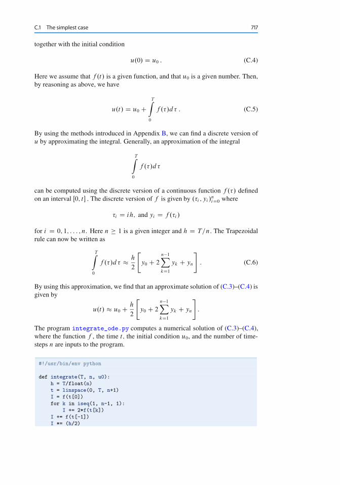
C.1 The simplest case 717
together with the initial condition
u.0/ D u0 : (C.4)
Here we assume that f .t/ is a given function, and that u0 is a given number. Then,by reasoning as above, we have
u.t/ D u0 CTZ
0
f .�/d� : (C.5)
By using the methods introduced in Appendix B, we can find a discrete version ofu by approximating the integral. Generally, an approximation of the integral
TZ
0
f .�/d�
can be computed using the discrete version of a continuous function f .�/ definedon an interval Œ0; t � : The discrete version of f is given by .�i ; yi /
niD0 where
�i D ih; and yi D f .�i /
for i D 0; 1; : : : ; n. Here n � 1 is a given integer and h D T=n: The Trapezoidalrule can now be written as
TZ
0
f .�/d� � h
2
"y0 C 2
n�1XkD1
yk C yn
#: (C.6)
By using this approximation, we find that an approximate solution of (C.3)–(C.4) isgiven by
u.t/ � u0 C h
2
"y0 C 2
n�1XkD1
yk C yn
#:
The program integrate_ode.py computes a numerical solution of (C.3)–(C.4),where the function f , the time t; the initial condition u0, and the number of time-steps n are inputs to the program.
#!/usr/bin/env python
def integrate(T, n, u0):
h = T/float(n)
t = linspace(0, T, n+1)
I = f(t[0])
for k in iseq(1, n-1, 1):
I += 2*f(t[k])
I += f(t[-1])
I *= (h/2)
718 C Introduction to differential equations
I += u0
return I
from scitools.std import *
f_formula = sys.argv[1]
T = eval(sys.argv[2])
u0 = eval(sys.argv[3])
n = int(sys.argv[4])
f = StringFunction(f_formula, independent_variables=’t’)
print "Numerical solution of u’(t)=%s: %.4f" % \
(f_formula, integrate(T, n, u0))
We apply the program for computing the solution of
u0.t/ D tet2
;
u.0/ D 0;
at time T D 2 using n D 10; 20; 50 and 100:
Terminal
Terminal> python src-ode1/integrate_ode.py ’t*exp(t**2)’ 2 0 10Numerical solution of u’(t)=t*exp(t**2): 28.4066
Terminal
Terminal> python src-ode1/integrate_ode.py ’t*exp(t**2)’ 2 0 20Numerical solution of u’(t)=t*exp(t**2): 27.2060
Terminal
Terminal> python src-ode1/integrate_ode.py ’t*exp(t**2)’ 2 0 50Numerical solution of u’(t)=t*exp(t**2): 26.8644
Terminal
Terminal> python src-ode1/integrate_ode.py ’t*exp(t**2)’ 2 0 100Numerical solution of u’(t)=t*exp(t**2): 26.8154
The exact solution is given by 12e22 � 1
2� 26:799; so we see that the approximate
solution becomes better as n is increased, as expected.
C.2 Exponential Growth
The example above was really not much of a differential equation, because thesolution was obtained by straightforward integration. Equations of the form
u0.t/ D f .t/ (C.7)
C.2 Exponential Growth 719
arise in situations where we can explicitly specify the derivative of the unknownfunction u: Usually, the derivative is specified in terms of the solution itself. Con-sider, for instance, population growth under idealized conditions as modeled inSect. A.1.4. We introduce the symbol vi for the number of individuals at time�i (vi corresponds to xn in Sect. A.1.4). The basic model for the evolution of vi is(A.9):
vi D .1 C r/vi�1; i D 1; 2; : : : ; and v0 known : (C.8)
As mentioned in Sect. A.1.4, r depends on the time difference �� D �i � �i�1: thelarger �� is, the larger r is. It is therefore natural to introduce a growth rate ˛ thatis independent of �� : ˛ D r=�� . The number ˛ is then fixed regardless of howlong jumps in time we take in the difference equation for vi . In fact, ˛ equals thegrowth in percent, divided by 100, over a time interval of unit length.
The difference equation now reads
vi D vi�1 C ˛�� vi�1 :
Rearranging this equation we get
vi � vi�1
��D ˛vi�1 : (C.9)
Assume now that we shrink the time step �� to a small value. The left-hand side of(C.9) is then an approximation to the time-derivative of a function v.�/ expressingthe number of individuals in the population at time � . In the limit �� ! 0, theleft-hand side becomes the derivative exactly, and the equation reads
v0.�/ D ˛v.�/ : (C.10)
As for the underlying difference equation, we need a start value v.0/ D v0. We haveseen that reducing the time step in a difference equation to zero, we get a differentialequation.
Many like to scale an equation like (C.10) such that all variables are withoutphysical dimensions and their maximum absolute value is typically of the orderof unity. In the present model, this means that we introduce new dimensionlessvariables
u D v
v0
; t D �
˛
and derive an equation for u.t/. Inserting v D v0u and � D ˛t in (C.10) gives theprototype equation for population growth:
u0.t/ D u.t/ (C.11)
with the initial conditionu.0/ D 1 : (C.12)
When we have computed the dimensionless u.t/, we can find the function v.�/ as
v.�/ D v0u.�=˛/ :
We shall consider practical applications of population growth equations later, butlet’s start by looking at the idealized case (C.11).
720 C Introduction to differential equations
Analytical solution Our differential equation can be written in the form
du
dtD u;
which can be rewritten asdu
uD dt;
and then integration on both sides yields
ln.u/ D t C c;
where c is a constant that has to be determined by using the initial condition. Puttingt D 0; we have
ln.u.0// D c;
hencec D ln.1/ D 0;
and thenln.u/ D t;
so we have the solutionu.t/ D et : (C.13)
Let us now check that this function really solves (C.7)–(C.11). Obviously, u.0/ De0 D 1; so (C.11) is fine. Furthermore
u0.t/ D et D u.t/;
thus (C.7) also holds.
Numerical solution We have seen that we can find a formula for the solution ofthe equation of exponential growth. So the problem is solved, and it is trivial towrite a program to graph the solution. We will, however, go one step further anddevelop a numerical solution strategy for this problem. We don’t really need sucha method for this problem since the solution is available in terms of a formula, butas mentioned earlier, it is good practice to develop methods for problems where weknow the solution; then we are more confident when we are confronted with morechallenging problems.
Suppose we want to compute a numerical approximation of the solution of
u0.t/ D u.t/ (C.14)
equipped with the initial condition
u.0/ D 1 : (C.15)
We want to compute approximations from time t D 0 to time t D 1. Let n � 1 bea given integer, and define
�t D 1=n : (C.16)
C.2 Exponential Growth 721
Furthermore, let uk denote an approximation of u.tk/ where
tk D k�t (C.17)
for k D 0; 1; : : : ; n. The key step in developing a numerical method for this differ-ential equation is to invoke the Taylor series as applied to the exact solution,
u.tkC1/ D u.tk/ C �tu0.tk/ C O.�t2/; (C.18)
which implies that
u0.tk/ � u.tkC1/ � u.tk/
�t: (C.19)
By using (C.14), we get
u.tkC1/ � u.tk/
�t� u.tk/ : (C.20)
Recall now that u.tk/ is the exact solution at time tk; and that uk is the approximatesolution at the same point in time. We now want to determine uk for all k � 0:
Obviously, we start by defining
u0 D u.0/ D 1:
Since we want uk � u.tk/; we require that uk satisfy the following equality
ukC1 � uk
�tD uk (C.21)
motivated by (C.20). It follows that
ukC1 D .1 C �t/uk : (C.22)
Since u0 is known, we can compute u1; u2 and so on by using the formula above.The formula is implemented in the program exp_growth.py. Actually, we do notneed the method and we do not need the program. It follows from (C.22) that
uk D .1 C �t/ku0
for k D 0; 1; : : : ; n which can be evaluated on a pocket calculator or even on yourcellular phone. But again, we show examples where everything is as simple aspossible (but not simpler!) in order to prepare your mind for more complex mattersahead.
#!/usr/bin/env python
def compute_u(u0, T, n):
"""Solve u’(t)=u(t), u(0)=u0 for t in [0,T] with n steps."""
u = u0
dt = T/float(n)
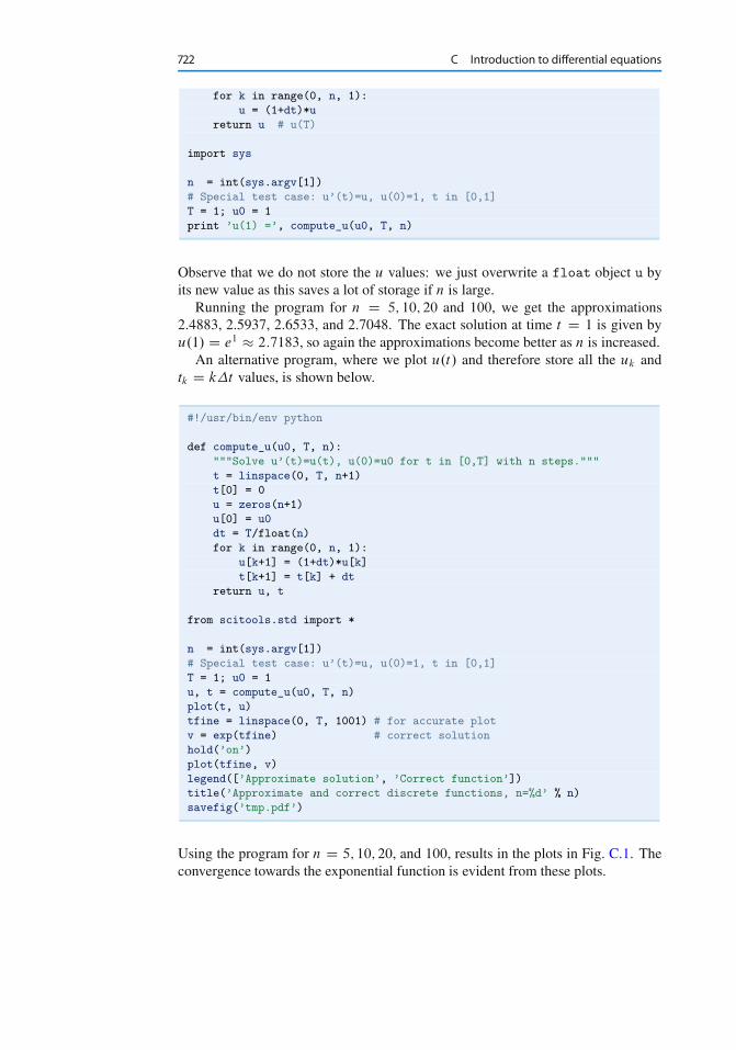
722 C Introduction to differential equations
for k in range(0, n, 1):
u = (1+dt)*u
return u # u(T)
import sys
n = int(sys.argv[1])
# Special test case: u’(t)=u, u(0)=1, t in [0,1]
T = 1; u0 = 1
print ’u(1) =’, compute_u(u0, T, n)
Observe that we do not store the u values: we just overwrite a float object u byits new value as this saves a lot of storage if n is large.
Running the program for n D 5; 10; 20 and 100, we get the approximations2.4883, 2.5937, 2.6533, and 2.7048. The exact solution at time t D 1 is given byu.1/ D e1 � 2:7183, so again the approximations become better as n is increased.
An alternative program, where we plot u.t/ and therefore store all the uk andtk D k�t values, is shown below.
#!/usr/bin/env python
def compute_u(u0, T, n):
"""Solve u’(t)=u(t), u(0)=u0 for t in [0,T] with n steps."""
t = linspace(0, T, n+1)
t[0] = 0
u = zeros(n+1)
u[0] = u0
dt = T/float(n)
for k in range(0, n, 1):
u[k+1] = (1+dt)*u[k]
t[k+1] = t[k] + dt
return u, t
from scitools.std import *
n = int(sys.argv[1])
# Special test case: u’(t)=u, u(0)=1, t in [0,1]
T = 1; u0 = 1
u, t = compute_u(u0, T, n)
plot(t, u)
tfine = linspace(0, T, 1001) # for accurate plot
v = exp(tfine) # correct solution
hold(’on’)
plot(tfine, v)
legend([’Approximate solution’, ’Correct function’])
title(’Approximate and correct discrete functions, n=%d’ % n)
savefig(’tmp.pdf’)
Using the program for n D 5; 10; 20, and 100, results in the plots in Fig. C.1. Theconvergence towards the exponential function is evident from these plots.
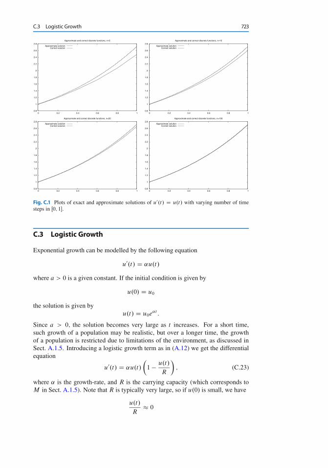
C.3 Logistic Growth 723
0.8
1
1.2
1.4
1.6
1.8
2
2.2
2.4
2.6
2.8
0 0.2 0.4 0.6 0.8 1
Approximate and correct discrete functions, n=5
Approximate solutionCorrect solution
0.8
1
1.2
1.4
1.6
1.8
2
2.2
2.4
2.6
2.8
0 0.2 0.4 0.6 0.8 1
Approximate and correct discrete functions, n=10
Approximate solutionCorrect solution
0.8
1
1.2
1.4
1.6
1.8
2
2.2
2.4
2.6
2.8
0 0.2 0.4 0.6 0.8 1
Approximate and correct discrete functions, n=20
Approximate solutionCorrect solution
0.8
1
1.2
1.4
1.6
1.8
2
2.2
2.4
2.6
2.8
0 0.2 0.4 0.6 0.8 1
Approximate and correct discrete functions, n=100
Approximate solutionCorrect solution
Fig. C.1 Plots of exact and approximate solutions of u0.t/ D u.t/ with varying number of timesteps in Œ0; 1�.
C.3 Logistic Growth
Exponential growth can be modelled by the following equation
u0.t/ D ˛u.t/
where a > 0 is a given constant. If the initial condition is given by
u.0/ D u0
the solution is given byu.t/ D u0e
˛t :
Since a > 0; the solution becomes very large as t increases. For a short time,such growth of a population may be realistic, but over a longer time, the growthof a population is restricted due to limitations of the environment, as discussed inSect. A.1.5. Introducing a logistic growth term as in (A.12) we get the differentialequation
u0.t/ D ˛u.t/
�1 � u.t/
R
�; (C.23)
where ˛ is the growth-rate, and R is the carrying capacity (which corresponds toM in Sect. A.1.5). Note that R is typically very large, so if u.0/ is small, we have
u.t/
R� 0
724 C Introduction to differential equations
for small values of t; and thus we have exponential growth for small t Iu0.t/ � au.t/:
But as t increases, and u grows, the term u.t/=R will become important and limitthe growth.
A numerical scheme for the logistic equation (C.23) is given by
ukC1 � uk
�tD ˛uk
�1 � uk
R
�;
which we can solve with respect to the unknown ukC1:
ukC1 D uk C �t˛uk
�1 � uk
R
�:
This is the form of the equation that is suited for implementation.
C.4 A Simple Pendulum
So far we have considered scalar ordinary differential equations, i.e., equations withone single function u.t/ as unknown. Now we shall deal with systems of ordinarydifferential equations, where in general n unknown functions are coupled in a sys-tem of n equations. Our introductory example will be a system of two equationshaving two unknown functions u.t/ and v.t/. The example concerns the motionof a pendulum, see Fig. C.2. A sphere with mass m is attached to a massless rodof length L and oscillates back and forth due to gravity. Newton’s second law ofmotion applied to this physical system gives rise the differential equation
00.t/ C ˛ sin./ D 0; (C.24)
where D .t/ is the angle the rod makes with the vertical, measured in radians,and ˛ D g=L (g is the acceleration of gravity). The unknown function to solvefor is , and knowing , we can quite easily compute the position of the sphere,its velocity, and its acceleration, as well as the tension force in the rod. Since thehighest derivative in (C.24) is of second order, we refer to (C.24) as a second-orderdifferential equations. Our previous examples in this chapter involved only first-order derivatives, and therefore they are known as first-order differential equations.
Equation (C.24) can be solved by the same numerical method as we use inSect. D.1.2, because (C.24) is very similar to Equation (D.8), which is the topicof Appendix D. The only difference is that (D.8) has extra terms, which can beskipped, while the kS term in (D.8) must be extended to ˛ sin.S/ to make (D.8)identical to (C.24). This extension is easily performed. However, here we shallnot solve the second-order equation (C.24) as it stands. We shall instead rewrite itas a system of two first-order equations so that we can use numerical methods forfirst-order equations to solve it.
To transform a second-order equation to a system of two first-order equations,we introduce a new variable for the first-order derivative (the angular velocity of thesphere): v.t/ D 0.t/. Using v and in (C.24) yields
v0.t/ C ˛ sin./ D 0 :
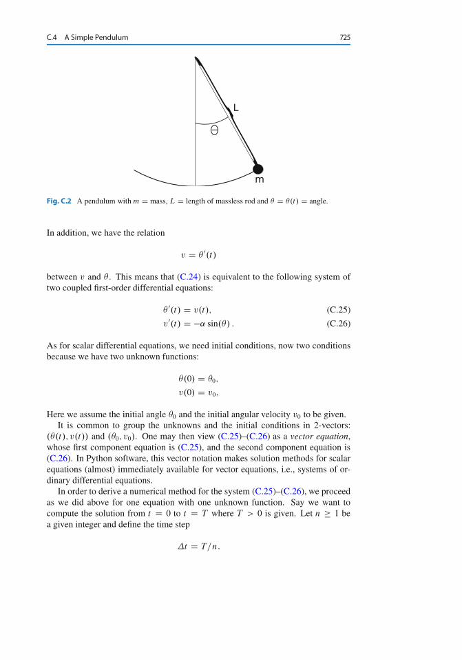
C.4 A Simple Pendulum 725
Fig. C.2 A pendulum with m D mass, L D length of massless rod and D .t/ D angle.
In addition, we have the relation
v D 0.t/
between v and . This means that (C.24) is equivalent to the following system oftwo coupled first-order differential equations:
0.t/ D v.t/; (C.25)
v0.t/ D �˛ sin./ : (C.26)
As for scalar differential equations, we need initial conditions, now two conditionsbecause we have two unknown functions:
.0/ D 0;
v.0/ D v0;
Here we assume the initial angle 0 and the initial angular velocity v0 to be given.It is common to group the unknowns and the initial conditions in 2-vectors:
..t/; v.t// and .0; v0/. One may then view (C.25)–(C.26) as a vector equation,whose first component equation is (C.25), and the second component equation is(C.26). In Python software, this vector notation makes solution methods for scalarequations (almost) immediately available for vector equations, i.e., systems of or-dinary differential equations.
In order to derive a numerical method for the system (C.25)–(C.26), we proceedas we did above for one equation with one unknown function. Say we want tocompute the solution from t D 0 to t D T where T > 0 is given. Let n � 1 bea given integer and define the time step
�t D T=n:
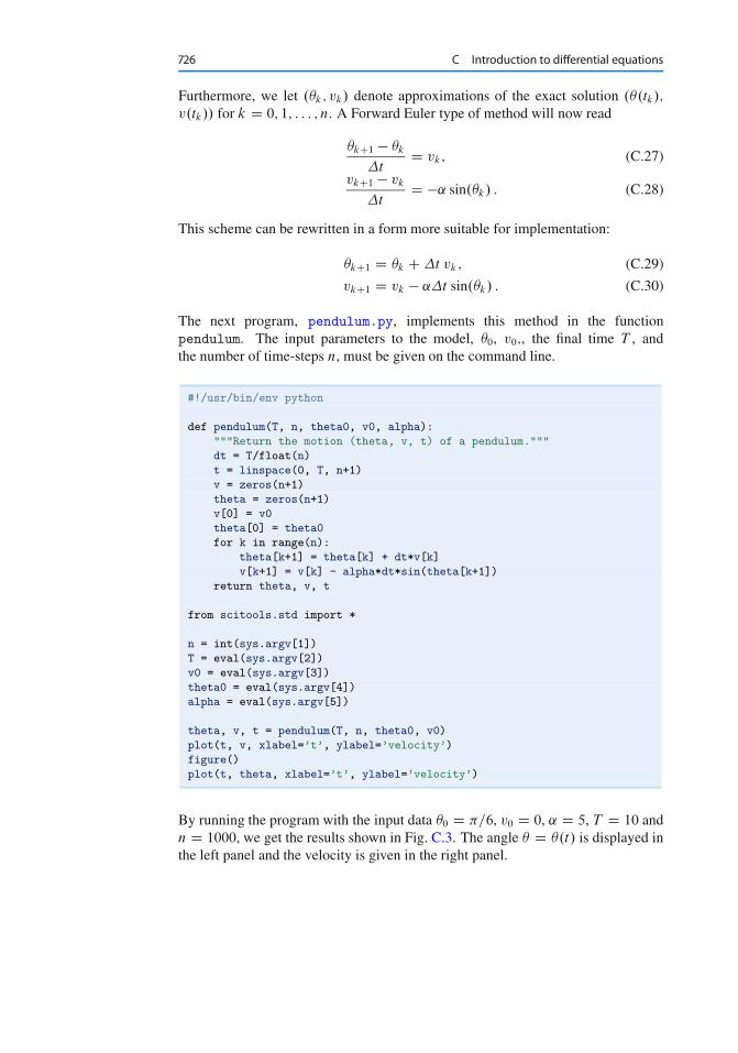
726 C Introduction to differential equations
Furthermore, we let .k; vk/ denote approximations of the exact solution ..tk/;
v.tk// for k D 0; 1; : : : ; n. A Forward Euler type of method will now read
kC1 � k
�tD vk; (C.27)
vkC1 � vk
�tD �˛ sin.k/ : (C.28)
This scheme can be rewritten in a form more suitable for implementation:
kC1 D k C �t vk; (C.29)
vkC1 D vk � ˛�t sin.k/ : (C.30)
The next program, pendulum.py, implements this method in the functionpendulum. The input parameters to the model, 0, v0;, the final time T , andthe number of time-steps n, must be given on the command line.
#!/usr/bin/env python
def pendulum(T, n, theta0, v0, alpha):
"""Return the motion (theta, v, t) of a pendulum."""
dt = T/float(n)
t = linspace(0, T, n+1)
v = zeros(n+1)
theta = zeros(n+1)
v[0] = v0
theta[0] = theta0
for k in range(n):
theta[k+1] = theta[k] + dt*v[k]
v[k+1] = v[k] - alpha*dt*sin(theta[k+1])
return theta, v, t
from scitools.std import *
n = int(sys.argv[1])
T = eval(sys.argv[2])
v0 = eval(sys.argv[3])
theta0 = eval(sys.argv[4])
alpha = eval(sys.argv[5])
theta, v, t = pendulum(T, n, theta0, v0)
plot(t, v, xlabel=’t’, ylabel=’velocity’)
figure()
plot(t, theta, xlabel=’t’, ylabel=’velocity’)
By running the program with the input data 0 D �=6, v0 D 0, ˛ D 5, T D 10 andn D 1000, we get the results shown in Fig. C.3. The angle D .t/ is displayed inthe left panel and the velocity is given in the right panel.
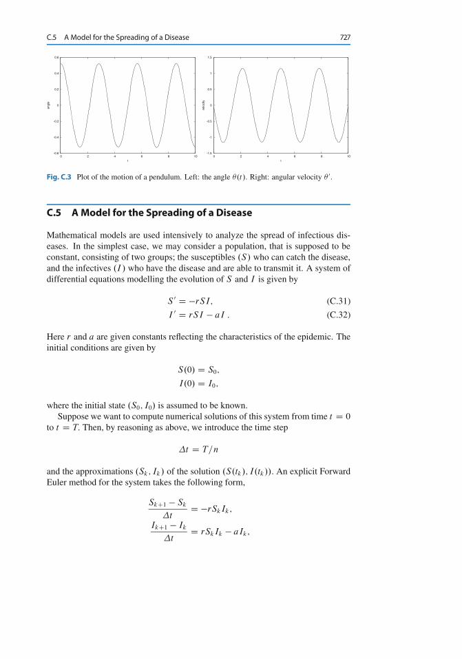
C.5 A Model for the Spreading of a Disease 727
-0.6
-0.4
-0.2
0
0.2
0.4
0.6
0 2 4 6 8 10
angl
e
t
-1.5
-1
-0.5
0
0.5
1
1.5
0 2 4 6 8 10
velo
city
t
Fig. C.3 Plot of the motion of a pendulum. Left: the angle .t/. Right: angular velocity 0.
C.5 AModel for the Spreading of a Disease
Mathematical models are used intensively to analyze the spread of infectious dis-eases. In the simplest case, we may consider a population, that is supposed to beconstant, consisting of two groups; the susceptibles .S/ who can catch the disease,and the infectives .I / who have the disease and are able to transmit it. A system ofdifferential equations modelling the evolution of S and I is given by
S 0 D �rSI; (C.31)
I 0 D rSI � aI : (C.32)
Here r and a are given constants reflecting the characteristics of the epidemic. Theinitial conditions are given by
S.0/ D S0;
I.0/ D I0;
where the initial state .S0; I0/ is assumed to be known.Suppose we want to compute numerical solutions of this system from time t D 0
to t D T: Then, by reasoning as above, we introduce the time step
�t D T=n
and the approximations .Sk; Ik/ of the solution .S.tk/; I.tk//: An explicit ForwardEuler method for the system takes the following form,
SkC1 � Sk
�tD �rSkIk;
IkC1 � Ik
�tD rSkIk � aIk;
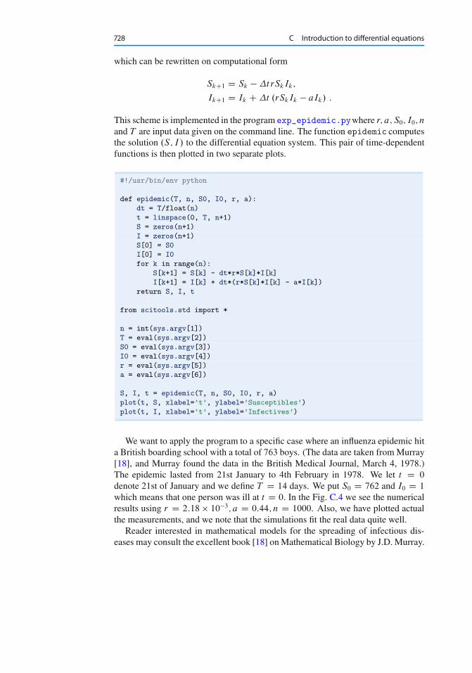
728 C Introduction to differential equations
which can be rewritten on computational form
SkC1 D Sk � �trSkIk;
IkC1 D Ik C �t .rSkIk � aIk/ :
This scheme is implemented in the program exp_epidemic.pywhere r; a; S0; I0; n
and T are input data given on the command line. The function epidemic computesthe solution .S; I / to the differential equation system. This pair of time-dependentfunctions is then plotted in two separate plots.
#!/usr/bin/env python
def epidemic(T, n, S0, I0, r, a):
dt = T/float(n)
t = linspace(0, T, n+1)
S = zeros(n+1)
I = zeros(n+1)
S[0] = S0
I[0] = I0
for k in range(n):
S[k+1] = S[k] - dt*r*S[k]*I[k]
I[k+1] = I[k] + dt*(r*S[k]*I[k] - a*I[k])
return S, I, t
from scitools.std import *
n = int(sys.argv[1])
T = eval(sys.argv[2])
S0 = eval(sys.argv[3])
I0 = eval(sys.argv[4])
r = eval(sys.argv[5])
a = eval(sys.argv[6])
S, I, t = epidemic(T, n, S0, I0, r, a)
plot(t, S, xlabel=’t’, ylabel=’Susceptibles’)
plot(t, I, xlabel=’t’, ylabel=’Infectives’)
We want to apply the program to a specific case where an influenza epidemic hita British boarding school with a total of 763 boys. (The data are taken fromMurray[18], and Murray found the data in the British Medical Journal, March 4, 1978.)The epidemic lasted from 21st January to 4th February in 1978. We let t D 0
denote 21st of January and we define T D 14 days. We put S0 D 762 and I0 D 1
which means that one person was ill at t D 0: In the Fig. C.4 we see the numericalresults using r D 2:18 � 10�3; a D 0:44; n D 1000. Also, we have plotted actualthe measurements, and we note that the simulations fit the real data quite well.
Reader interested in mathematical models for the spreading of infectious dis-eases may consult the excellent book [18] onMathematical Biology by J.D. Murray.
C.6 Exercises 729
0
100
200
300
400
500
600
700
800
0 2 4 6 8 10 12 14
Sus
cept
ible
s
t
0
50
100
150
200
250
300
0 2 4 6 8 10 12 14
Infe
ctiv
es
t
Numerical SolutionMeasured data
Fig. C.4 Graphs of susceptibles (left) and infectives (right) for an influenza in a British boardingschool in 1978.
C.6 Exercises
Exercise C.1: Solve a nonhomogeneous linear ODESolve the ODE problem
u0 D 2u � 1; u.0/ D 2; t 2 Œ0; 6�
using the Forward Euler method. Choose �t D 0:25. Plot the numerical solutiontogether with the exact solution u.t/ D 1
2C 3
2e2t .
Filename: nonhomogeneous_linear_ODE.
Exercise C.2: Solve a nonlinear ODESolve the ODE problem
u0 D uq; u.0/ D 1; t 2 Œ0; T �
using the Forward Euler method. The exact solution reads u.t/ D et for q D 1
and u.t/ D .t.1 � q/ C 1/1=.1�q/ for q > 1 and t.1 � q/ C 1 > 0. Read q, �t ,and T from the command line, solve the ODE, and plot the numerical and exactsolution. Run the program for different cases: q D 2 and q D 3, with �t D 0:01
and �t D 0:1. Set T D 6 if q D 1 and T D 1=.q � 1/ � 0:1 otherwise.Filename: nonlinear_ODE.
Exercise C.3: Solve an ODE for y.x/
We have given the following ODE problem:
dy
dxD 1
2.y � 1/; y.0/ D 1 C p
�; x 2 Œ0; 4�; (C.33)
where � > 0 is a small number. Formulate a Forward Euler method for this ODEproblem and compute the solution for varying step size in x: �x D 1, �x D 0:25,�x D 0:01. Plot the numerical solutions together with the exact solution y.x/ D1 C p
x C �, using 1001 x coordinates for accurate resolution of the latter. Set �
to 10�3. Study the numerical solution with �x D 1, and use that insight to explainwhy this problem is hard to solve numerically.Filename: yx_ODE.
730 C Introduction to differential equations
Exercise C.4: Experience instability of an ODEConsider the ODE problem
u0 D ˛u; u.0/ D u0;
solved by the Forward Euler method. Show by repeatedly applying the scheme that
uk D .1 C ˛�t/ku0 :
We now turn to the case ˛ < 0. Show that the numerical solution will oscillate if�t > �1=˛. Make a program for computing uk, set ˛ D �1, and demonstrateoscillatory solutions for �t D 1:1; 1:5; 1:9. Recall that the exact solution, u.t/ De˛t , never oscillates.
What happens if �t > �2=˛? Try it out in the program and explain why we donot experience that uk ! 0 as k ! 1.Filename: unstable_ODE.
Exercise C.5: Solve an ODE with time-varying growthConsider the ODE for exponential growth,
u0 D ˛u; u.0/ D 1; t 2 Œ0; T � :
Now we introduce a time-dependent ˛ such that the growth decreases with time:˛.t/ D a � bt . Solve the problem for a D 1, b D 0:1, and T D 10. Plot thesolution and compare with the corresponding exponential growth using the meanvalue of ˛.t/ as growth factor: e.a�bT=2/t .Filename: time_dep_growth.
DAComplete Differential Equation Project
The examples in the ordinary chapters of this book are quite compact and composedto convey programming constructs in a gentle pedagogical way. In this appendix theidea is to solve a more comprehensive real-world problem by programming. Theproblem solving process gets quite advanced because we bring together elementsfrom physics, mathematics, and programming, in a way that a scientific program-mer must master. Each individual element is quite straightforward in the sense thatyou have probably met the element already, either in high school physics or mathe-matics, or in this book. The challenge is to understand the problem, and analyze itby breaking it into a set of simpler elements. It is not necessary to understand thisproblem solving process in detail. As a computer programmer, all you need to un-derstand is how you translate the given algorithm into a working program and howto test the program. We anticipate that this task should be doable without a thoroughunderstanding of the physics and mathematics of the problem.
Sections D.1 and D.2 require basic knowledge of loops, lists, functions, andcommand-line parsing via the argparse module, while Sect. D.3 also requiresknowledge about curve plotting.
All Python files associated with this appendix are found in src/boxspring1.
D.1 About the Problem: Motion and Forces in Physics
D.1.1 The Physical Problem
We shall study a simple device for modeling oscillating systems. A boxwith massm
and height b is attached to a spring of length L as shown in Fig. D.1. The end of thespring is attached to a plate, which we can move up and down with a displacementw.t/, where t denotes time. There are two ways the box can be set in motion: wecan either stretch or compress the string initially by moving the box up or down, orwe can move the plate. If w D 0 the box oscillates freely, otherwise we have whatis called driven oscillations.
Why will such a system oscillate? When the box moves downward, the springis stretched, which results in a force that tries to move the box upward. The more
1 http://tinyurl.com/pwyasaa/boxspring
731
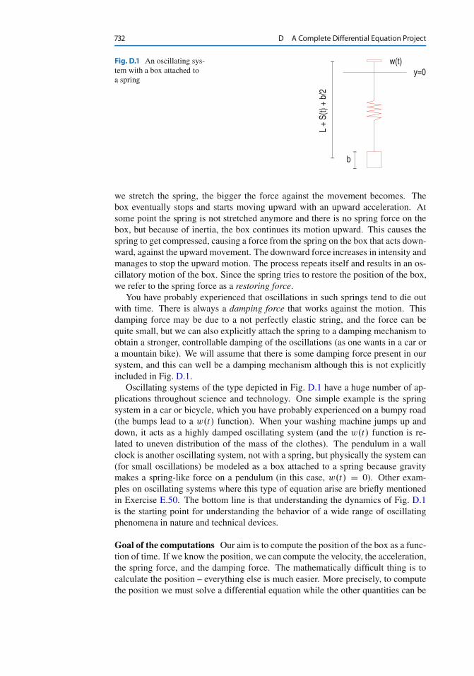
732 D A Complete Differential Equation Project
Fig. D.1 An oscillating sys-tem with a box attached toa spring
we stretch the spring, the bigger the force against the movement becomes. Thebox eventually stops and starts moving upward with an upward acceleration. Atsome point the spring is not stretched anymore and there is no spring force on thebox, but because of inertia, the box continues its motion upward. This causes thespring to get compressed, causing a force from the spring on the box that acts down-ward, against the upward movement. The downward force increases in intensity andmanages to stop the upward motion. The process repeats itself and results in an os-cillatory motion of the box. Since the spring tries to restore the position of the box,we refer to the spring force as a restoring force.
You have probably experienced that oscillations in such springs tend to die outwith time. There is always a damping force that works against the motion. Thisdamping force may be due to a not perfectly elastic string, and the force can bequite small, but we can also explicitly attach the spring to a damping mechanism toobtain a stronger, controllable damping of the oscillations (as one wants in a car ora mountain bike). We will assume that there is some damping force present in oursystem, and this can well be a damping mechanism although this is not explicitlyincluded in Fig. D.1.
Oscillating systems of the type depicted in Fig. D.1 have a huge number of ap-plications throughout science and technology. One simple example is the springsystem in a car or bicycle, which you have probably experienced on a bumpy road(the bumps lead to a w.t/ function). When your washing machine jumps up anddown, it acts as a highly damped oscillating system (and the w.t/ function is re-lated to uneven distribution of the mass of the clothes). The pendulum in a wallclock is another oscillating system, not with a spring, but physically the system can(for small oscillations) be modeled as a box attached to a spring because gravitymakes a spring-like force on a pendulum (in this case, w.t/ D 0). Other exam-ples on oscillating systems where this type of equation arise are briefly mentionedin Exercise E.50. The bottom line is that understanding the dynamics of Fig. D.1is the starting point for understanding the behavior of a wide range of oscillatingphenomena in nature and technical devices.
Goal of the computations Our aim is to compute the position of the box as a func-tion of time. If we know the position, we can compute the velocity, the acceleration,the spring force, and the damping force. The mathematically difficult thing is tocalculate the position – everything else is much easier. More precisely, to computethe position we must solve a differential equation while the other quantities can be
D.1 About the Problem: Motion and Forces in Physics 733
computed by differentiation and simple arithmetics. Solving differential equationsis historically considered very difficult, but computers have simplified this task dra-matically.
We assume that the boxmoves in the vertical direction only, so we introduce Y.t/
as the vertical position of the center point of the box. We shall derive a mathematicalequation that has Y.t/ as solution. This equation can be solved by an algorithm,which can be implemented in a program. Our focus is on the implementation, sincethis is a book about programming, but for the reader interested in how computersplay together with physics and mathematics in science and technology, we alsooutline how the equation and algorithm arise.
The key quantities Let S be the stretch of the spring, where S > 0 means stretchand S < 0 implies compression. The length of the spring when it is unstretched isL, so at a given point of time t the actual length is L C S.t/. Given the position ofthe plate, w.t/, the length of the spring, L C S.t/, and the height of the box, b, theposition Y.t/ is then, according to Fig. D.1,
Y.t/ D w.t/ � .L C S.t// � b
2: (D.1)
You can think as follows: we first “go up” to the plate at y D w.t/, then downL C S.t/ along the spring and then down b=2 to the center of the box. While L, w,and b must be known as input data, S.t/ is unknown and will be output data fromthe program.
D.1.2 The Computational Algorithm
Let us now go straight to the programming task and present the recipe for computingY.t/. The algorithm below actually computes S.t/, but at any point of time we caneasily find Y.t/ from (D.1) if we know S.t/. The S.t/ function is computed atdiscrete points of time, t D ti D i�t , for i D 0; 1; : : : ; N . We introduce thenotation Si for S.ti /. The Si values can be computed by the following algorithm.
Set the initial stretch S0 from input data and compute S1 by
SiC1 D 1
2m
�2mSi � �t2 kSi C m .wiC1 � 2wi C wi�1/ C �t2 mg
�; (D.2)
with i D 0. Then for i D 1; 2; : : : ; N � 1, compute SiC1 by
SiC1 D .m C �/�1�2mSi � mSi�1 C ��t Si�1 � �t2 kSiC
m.wiC1 � 2wi C wi�1/ C �t2 mg�
: (D.3)
The parameter � equals 12ˇ�t . The input data to the algorithm are the mass of
the box m, a coefficient k characterizing the spring, a coefficient ˇ characterizingthe amount of damping in the system, the acceleration of gravity g, the movementof the plate w.t/, the initial stretch of the spring S0, the number of time steps N ,and the time �t between each computation of S values. The smaller we choose �t ,the more accurate the computations become.
734 D A Complete Differential Equation Project
Now you have two options, either read the derivation of this algorithm inSects. D.1.3 and D.1.4 or jump right to implementation in Sect. D.2.
D.1.3 Derivation of theMathematical Model
To derive the algorithm we need to make a mathematical model of the oscillatingsystem. This model is based on physical laws. The most important physical law fora moving body is Newton’s second law of motion:
F D ma; (D.4)
where F is the sum of all forces on the body, m is the mass of the body, and a is theacceleration of the body. The body here is our box.
Let us first find all the forces on the box. Gravity acts downward with magnitudemg. We introduce Fg D �mg as the gravity force, with a minus sign becausea negative force acts downward, in negative y direction.
The spring force on the box acts upward if the spring is stretched, i.e., if S > 0
we have a positive spring force Fs . The size of the force is proportional to theamount of stretching, so we write Fs D kS , where k is commonly known as thespring constant. (Spring forces are often written in the canonical form F D �kx,where x is the stretch. The reason that we have no minus sign is that our stretchS is positive in the downward, negative direction.) We also assume that we havea damping force that is always directed toward the motion and proportional withthe velocity of the stretch, �dS=dt . Naming the proportionality constant ˇ, we canwrite the damping force as Fd D ˇdS=dt . Note that when dS=dt > 0, S increasesin time and the box moves downward, the Fd force then acts upward, against themotion, and must be positive. This is the way we can check that the damping forceexpression has the right sign.
The sum of all forces is now
F D Fg C Fs C Fd ;
D �mg C kS C ˇdS
dt: (D.5)
We now know the left-hand side of (D.4), but S is unknown to us. The acceler-ation a on the right-hand side of (D.4) is also unknown. However, acceleration isrelated to movement and the S quantity, and through this relation we can eliminatea as a second unknown. From physics, it is known that the acceleration of a bodyis the second derivative in time of the position of the body, so in our case,
a D d 2Y
dt2;
D d 2w
dt2� d 2S
dt2; (D.6)
(remember that L and b are constant).
D.1 About the Problem: Motion and Forces in Physics 735
Equation (D.4) now reads
� mg C kS C ˇdS
dtD m
�d 2w
dt2� d 2S
dt2
�: (D.7)
It is common to collect the unknown terms on the left-hand side and the knownquantities on the right-hand side, and let higher-order derivatives appear beforelower-order derivatives. With such a reordering of terms we get
md 2S
dt2C ˇ
dS
dtC kS D m
d 2w
dt2C mg : (D.8)
This is the equation governing our physical system. If we solve the equation forS.t/, we have the position of the box according to (D.1), the velocity v as
v.t/ D dY
dtD dw
dt� dS
dt; (D.9)
the acceleration as (D.6), and the various forces can be easily obtained from theformulas in (D.5).
A key question is if we can solve (D.8). If w D 0, there is in fact a well-knownsolution, which can be written
S.t/ D m
kg C
8̂<̂ˆ̂:
e�t�c1e
tp
ˇ2�1 C c2e�t
p2�1
�; > 1;
e�t .c1 C c2t/; D 1;
e�thc1 cos
�p1 � 2t
�C c2 sin
�p1 � 2t
�i; < 1 :
(D.10)Here, is a short form for ˇ=2, and c1 and c2 are arbitrary constants. That is, thesolution (D.10) is not unique.
To make the solution unique, we must determine c1 and c2. This is done byspecifying the state of the system at some point of time, say t D 0. In the presenttype of mathematical problem we must specify S and dS=dt . We allow the springto be stretched an amount S0 at t D 0. Moreover, we assume that there is noongoing increase or decrease in the stretch at t D 0, which means that dS=dt D 0.In view of (D.9), this condition implies that the velocity of the box is that of theplate, and if the latter is at rest, the box is also at rest initially. The conditions att D 0 are called initial conditions:
S.0/ D S0;dS
dt.0/ D 0 : (D.11)
These two conditions provide two equations for the two unknown constants c1 andc2. Without the initial conditions two things happen: (i) there are infinitely manysolutions to the problem, and (ii) the computational algorithm in a program cannotstart.
Also when w ¤ 0 one can find solutions S.t/ of (D.8) in terms of mathemat-ical expressions, but only for some very specific choices of w.t/ functions. Witha program we can compute the solution S.t/ for any “reasonable” w.t/ by a quitesimple method. The method gives only an approximate solution, but the approxi-mation can usually be made as good as desired. This powerful solution method isdescribed below.
736 D A Complete Differential Equation Project
D.1.4 Derivation of the Algorithm
To solve (D.8) on a computer, we do two things:
We calculate the solution at some discrete time points t D ti D i�t , i D0; 1; 2; : : : ; N .
We replace the derivatives by finite differences, which are approximate expres-sions for the derivatives.
The first and second derivatives can be approximated by the following finite differ-ences
dS
dt.ti / � S.tiC1/ � S.ti�1/
2�t; (D.12)
d 2S
dt2.ti / � S.tiC1/ � 2S.ti / C S.ti�1/
�t2: (D.13)
Derivations of such formulas can be found in Appendices B and C. It is common tosave some writing by introducing Si as a short form for S.ti /. The formulas thenread
dS
dt.ti / � SiC1 � Si�1
2�t; (D.14)
d 2S
dt2.ti / � SiC1 � 2Si C Si�1
�t2: (D.15)
Let (D.8) be valid at a point of time ti :
md 2S
dt2.ti / C ˇ
dS
dt.ti / C kS.ti / D m
d 2w
dt2.ti / C mg : (D.16)
We now insert (D.14) and (D.15) in (D.16) (observe that we can approximated 2w=dt2 in the same way as we approximate d 2S=dt2):
mSiC1 � 2Si C Si�1
�t2C ˇ
SiC1 � Si�1
2�tC kSi D m
wiC1 � 2wi C wi�1
�t2C mg :
(D.17)The computational algorithm starts with knowing S0, then S1 is computed, thenS2, and so on. Therefore, in (D.17) we can assume that Si and Si�1 are alreadycomputed, and that SiC1 is the new unknown to calculate. Let us as usual put theunknown terms on the left-hand side (and multiply by �t2):
mSiC1 C �SiC1 D 2mSi � mSi�1 C �Si�1 � �t2 kSiCm .wiC1 � 2wi C wi�1/ C �t2 mg; (D.18)
where we have introduced the short form � D 12ˇ�t to save space. Equation (D.18)
can easily be solved for SiC1:
SiC1 D .m C �/�1�2mSi � mSi�1 C �Si�1 � �t2 kSi Cm.wiC1 � 2wi C wi�1/ C �t2 mg
�; (D.19)
D.2 Program Development and Testing 737
One fundamental problem arises when we try to start the computations. Weknow S0 and want to apply (D.19) for i D 0 to calculate S1. However, (D.19)involves Si�1, that is, S�1, which is an unknown value at a point of time before wecompute the motion. The initial conditions come to rescue here. Since dS=dt D 0
at t D 0 (or i D 0), we can approximate this condition as
S1 � S�1
2�tD 0 ) S�1 D S1 : (D.20)
Inserting this relation in (D.19) when i D 0 gives a special formula for S1 (or SiC1
with i D 0, if we want):
SiC1 D 1
2m
�2mSi � �t2 kSi C m .wiC1 � 2wi C wi�1/ C �t2 mg
�: (D.21)
Remember that i D 0 in this formula. The overall algorithm is summarized below.
1. Initialize S0 from initial condition2. Use (D.21) to compute SiC1 for i D 0
3. For i D 0; 1; 2; : : : ; N � 1, use (D.19) to compute SiC1
D.2 Program Development and Testing
D.2.1 Implementation
The aim now is to implement the algorithm from Sect. D.1.2 in a Python program.There are naturally two parts of the program, one where we read input data suchas L, m, and w.t/, and one part where we run the computational algorithm. Let uswrite a function for each part.
The set of input data to the program consists of the mathematical symbols
m (the mass of the box) b (the height of the box) L (the length of the unstretched spring) ˇ (coefficient for the damping force) k (coefficient for the spring force) �t (the time step between each Si calculation) N (the number of computed time steps) S0 (the initial stretch of the spring) w.t/ (the vertical displacement of the plate) g (acceleration of gravity)
We make a function init_prms for initializing these input parameters from option-value pairs on the command line. That is, the user provides pairs like –m 2 and –dt0.1 (for �t). The argparse module from Sect. 4.4 can be used for this purpose.We supply default values for all parameters as arguments to the init_prms func-tion. The function returns all these parameters with the changes that the user hasspecified on the command line. The w parameter is given as a string expression
738 D A Complete Differential Equation Project
(called w_formula below), and the StringFunction tool from Sect. 4.3.3 can beused to turn the formula into a working Python function. An algorithmic sketchof the tasks in the init_prms function can be expressed by some pseudo Pythoncode:
def init_prms(m, b, L, k, beta, S0, dt, g, w_formula, N):
import argparse
parser = argparse.ArgumentParser()
parser.add_argument(’--m’, ’--mass’,
type=float, default=m)
parser.add_argument(’--b’, ’--boxheight’,
type=float, default=b)
...
args = parser.parse_args()
from scitools.StringFunction import StringFunction
w = StringFunction(args.w, independent_variables=’t’)
return args.m, args.b, args.L, args.k, args.beta, \
args.S0, args.dt, args.g, w, args.N
With such a sketch as a start, we can complete the indicated code and arrive ata working function for specifying input parameters to the mathematical model:
def init_prms(m, b, L, k, beta, S0, dt, g, w_formula, N):
import argparse
parser = argparse.ArgumentParser()
parser.add_argument(’--m’, ’--mass’,
type=float, default=m)
parser.add_argument(’--b’, ’--boxheight’,
type=float, default=b)
parser.add_argument(’--L’, ’--spring-length’,
type=float, default=L)
parser.add_argument(’--k’, ’--spring-stiffness’,
type=float, default=k)
parser.add_argument(’--beta’, ’--spring-damping’,
type=float, default=beta)
parser.add_argument(’--S0’, ’--initial-position’,
type=float, default=S0)
parser.add_argument(’--dt’,’--timestep’,
type=float, default=dt)
parser.add_argument(’--g’, ’--gravity’,
type=float, default=g)
parser.add_argument(’--w’, type=str, default=w_formula)
parser.add_argument(’--N’, type=int, default=N)
args = parser.parse_args()
from scitools.StringFunction import StringFunction
w = StringFunction(args.w, independent_variables=’t’)
return args.m, args.b, args.L, args.k, args.beta, \
args.S0, args.dt, args.g, w, args.N
You may wonder why we specify g (gravity) since this is a known constant, butit is useful to turn off the gravity force to test the program. Just imagine the oscil-lations take place in the horizontal direction – the mathematical model is the same,
D.2 Program Development and Testing 739
but Fg D 0, which we can obtain in our program by setting the input parameter gto zero.
The computational algorithm is quite easy to implement, as there is a quite directtranslation of the mathematical algorithm in Sect. D.1.2 to valid Python code. TheSi values can be stored in a list or array with indices going from 0 to N . We uselists and instead of arrays here to allow readers not familiar with the latter conceptto follow the code.
The function for computing Si reads
def solve(m, k, beta, S0, dt, g, w, N):
S = [0.0]*(N+1) # output list
gamma = beta*dt/2.0 # short form
t = 0
S[0] = S0
# Special formula for first time step
i = 0
S[i+1] = (1/(2.0*m))*(2*m*S[i] - dt**2*k*S[i] +
m*(w(t+dt) - 2*w(t) + w(t-dt)) + dt**2*m*g)
t = dt
for i in range(1,N):
S[i+1] = (1/(m + gamma))*(2*m*S[i] - m*S[i-1] +
gamma*dt*S[i-1] - dt**2*k*S[i] +
m*(w(t+dt) - 2*w(t) + w(t-dt))
+ dt**2*m*g)
t += dt
return S
The primary challenge in coding the algorithm is to set the index i and the timet right. Recall that in the updating formula for S[i+1] at time t+dt, the time onthe right-hand side shall be the time at time step i, so the t+=dt update must comeafter S[i+1] is computed. The same is important in the special formula for the firsttime step as well.
A main program will typically first set some default values of the 10 input pa-rameters, then call init_prms to let the user adjust the default values, and then callsolve to compute the Si values:
# Default values
from math import pi
m = 1; b = 2; L = 10; k = 1; beta = 0; S0 = 1;
dt = 2*pi/40; g = 9.81; w_formula = ’0’; N = 80;
m, b, L, k, beta, S0, dt, g, w, N = \
init_prms(m, b, L, k, beta, S0, dt, g, w_formula, N)
S = solve(m, k, beta, S0, dt, g, w, N)
So, what shall we do with the solution S? We can write out the values of this list,but the numbers do not give an immediate feeling for how the box moves. It will bebetter to graphically illustrate the S.t/ function, or even better, the Y.t/ function.This is straightforward and treated in Sect. D.3. In Sect. 9.4, we develop a drawingtool for drawing figures like Fig. D.1. By drawing the box, string, and plate atevery time level we compute Si , we can use this tool to make a moving figure that
740 D A Complete Differential Equation Project
illustrates the dynamics of the oscillations. Already now you can play around witha program doing that (boxspring_figure_anim.py).
D.2.2 Callback Functionality
It would be nice to make some graphics of the system while the computations takeplace, not only after the S list is ready. The user must then put some relevant state-ments in between the statements in the algorithm. However, such modificationswill depend on what type of analysis the user wants to do. It is a bad idea to mixuser-specific statements with general statements in a general algorithm. We there-fore let the user provide a function that the algorithm can call after each Si value iscomputed. This is commonly called a callback function (because a general functioncalls back to the user’s program to do a user-specific task). To this callback func-tion we send three key quantities: the S list, the point of time (t), and the time stepnumber (i C 1), so that the user’s code gets access to these important data.
If we just want to print the solution to the screen, the callback function can be assimple as
def print_S(S, t, step):
print ’t=%.2f S[%d]=%+g’ % (t, step, S[step])
In the solve function we take the callback function as a keyword argumentuser_action. The default value can be an empty function, which we can de-fine separately:
def empty_func(S, time, time_step_no):
return None
def solve(m, k, beta, S0, dt, g, w, N,
user_action=empty_func):
...
However, it is quicker to just use a lambda function (see Sect. 3.1.14):
def solve(m, k, beta, S0, dt, g, w, N,
user_action=lambda S, time, time_step_no: None):
The new solve function has a call to user_action each time a new S value hasbeen computed:
def solve(m, k, beta, S0, dt, g, w, N,
user_action=lambda S, time, time_step_no: None):
"""Calculate N steps forward. Return list S."""
S = [0.0]*(N+1) # output list
gamma = beta*dt/2.0 # short form
t = 0
S[0] = S0
user_action(S, t, 0)
# Special formula for first time step
i = 0
D.2 Program Development and Testing 741
S[i+1] = (1/(2.0*m))*(2*m*S[i] - dt**2*k*S[i] +
m*(w(t+dt) - 2*w(t) + w(t-dt)) + dt**2*m*g)
t = dt
user_action(S, t, i+1)
# Time loop
for i in range(1,N):
S[i+1] = (1/(m + gamma))*(2*m*S[i] - m*S[i-1] +
gamma*dt*S[i-1] - dt**2*k*S[i] +
m*(w(t+dt) - 2*w(t) + w(t-dt))
+ dt**2*m*g)
t += dt
user_action(S, t, i+1)
return S
def test_constant():
"""Test constant solution."""
from math import pi
m = 10.0; k = 5.0; g = 9.81;
S0 = m/k*g
m, b, L, k, beta, S0, dt, g, w, N = \
init_prms(m=10, b=0, L=5, k=5, beta=0, S0=S0,
dt=2*pi/40, g=g, w_formula=’0’, N=40)
S = solve(m, k, beta, S0, dt, g, w, N)
S_ref = S0 # S[i] = S0 is the reference value
tol = 1E-13
for S_ in S:
assert abs(S_ref - S_) < tol
def test_general_solve():
def print_S(S, t, step):
print ’t=%.2f S[%d]=%+g’ % (t, step, S[step])
# Default values
from math import pi
m = 1; b = 2; L = 10; k = 1; beta = 0; S0 = 1;
dt = 2*pi/40; g = 9.81; w_formula = ’0’; N = 80;
m, b, L, k, beta, S0, dt, g, w, N = \
init_prms(m, b, L, k, beta, S0, dt, g, w_formula, N)
S = solve(m, k, beta, S0, dt, g, w, N,
user_action=print_S)
S_reference = [
1, 1.1086890184669964, 1.432074279830456, 1.9621765725933782,
2.685916146951562, 3.5854354446841863]
for S_new, S_ref in zip(S, S_reference):
assert abs(S_ref - S_new) < 1E-14
def demo():
def print_S(S, t, step):
"""Callback function: user_action."""
print ’t=%.2f S[%d]=%+g’ % (t, step, S[step])
from math import pi
742 D A Complete Differential Equation Project
m, b, L, k, beta, S0, dt, g, w, N = \
init_prms(m=1, b=2, L=10, k=1, beta=0, S0=0,
dt=2*pi/40, g=9.81, w_formula=’0’, N=80)
S = solve(m, k, beta, S0, dt, g, w, N,
user_action=print_S)
import matplotlib.pyplot as plt
plt.plot(S)
plt.show()
if __name__ == ’__main__’:
#demo()
test_constant()
The two last arguments to user_actionmust be carefully set: these should betime value and index for the most recently computed S value.
D.2.3 Making aModule
The init_prms and solve functions can now be combined with many differenttypes of main programs and user_action functions. It is therefore preferable tohave the general init_prms and solve functions in a module boxspring andimport these functions in more user-specific programs. Making a module out ofinit_prms and solve is, according to Sect. 4.9, quite trivial as we just need to putthe functions in a file boxspring.py.
It is a good habit to include a demo function that quickly tells users how tooperate the key functions in the module. The demo function is often called from thetest block. Here is an example:
def demo():
def print_S(S, t, step):
"""Callback function: user_action."""
print ’t=%.2f S[%d]=%+g’ % (t, step, S[step])
from math import pi
m, b, L, k, beta, S0, dt, g, w, N = \
init_prms(m=1, b=2, L=10, k=1, beta=0, S0=0,
dt=2*pi/40, g=9.81, w_formula=’0’, N=80)
S = solve(m, k, beta, S0, dt, g, w, N,
user_action=print_S)
import matplotlib.pyplot as plt
plt.plot(S)
plt.show()
if __name__ == ’__main__’:
#demo()
test_constant()
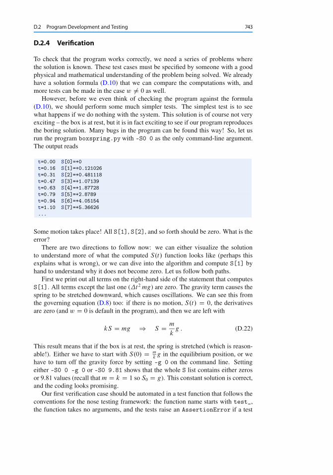
D.2 Program Development and Testing 743
D.2.4 Verification
To check that the program works correctly, we need a series of problems wherethe solution is known. These test cases must be specified by someone with a goodphysical and mathematical understanding of the problem being solved. We alreadyhave a solution formula (D.10) that we can compare the computations with, andmore tests can be made in the case w ¤ 0 as well.
However, before we even think of checking the program against the formula(D.10), we should perform some much simpler tests. The simplest test is to seewhat happens if we do nothing with the system. This solution is of course not veryexciting – the box is at rest, but it is in fact exciting to see if our program reproducesthe boring solution. Many bugs in the program can be found this way! So, let usrun the program boxspring.py with –S0 0 as the only command-line argument.The output reads
t=0.00 S[0]=+0
t=0.16 S[1]=+0.121026
t=0.31 S[2]=+0.481118
t=0.47 S[3]=+1.07139
t=0.63 S[4]=+1.87728
t=0.79 S[5]=+2.8789
t=0.94 S[6]=+4.05154
t=1.10 S[7]=+5.36626
...
Some motion takes place! All S[1], S[2], and so forth should be zero. What is theerror?
There are two directions to follow now: we can either visualize the solutionto understand more of what the computed S.t/ function looks like (perhaps thisexplains what is wrong), or we can dive into the algorithm and compute S[1] byhand to understand why it does not become zero. Let us follow both paths.
First we print out all terms on the right-hand side of the statement that computesS[1]. All terms except the last one (�t2 mg) are zero. The gravity term causes thespring to be stretched downward, which causes oscillations. We can see this fromthe governing equation (D.8) too: if there is no motion, S.t/ D 0, the derivativesare zero (and w D 0 is default in the program), and then we are left with
kS D mg ) S D m
kg : (D.22)
This result means that if the box is at rest, the spring is stretched (which is reason-able!). Either we have to start with S.0/ D m
kg in the equilibrium position, or we
have to turn off the gravity force by setting –g 0 on the command line. Settingeither –S0 0 –g 0 or –S0 9.81 shows that the whole S list contains either zerosor 9.81 values (recall that m D k D 1 so S0 D g). This constant solution is correct,and the coding looks promising.
Our first verification case should be automated in a test function that follows theconventions for the nose testing framework: the function name starts with test_,the function takes no arguments, and the tests raise an AssertionError if a test
744 D A Complete Differential Equation Project
fails (e.g., by using assert success, where success is a boolean variable re-flecting whether the test is successful or not).
A relevant test function sets the special input corresponding to the equilibriumposition and must test that every S[i] equals the constant reference value withina tolerance:
def test_constant():
"""Test constant solution."""
from math import pi
m = 10.0; k = 5.0; g = 9.81;
S0 = m/k*g
m, b, L, k, beta, S0, dt, g, w, N = \
init_prms(m=10, b=0, L=5, k=5, beta=0, S0=S0,
dt=2*pi/40, g=g, w_formula=’0’, N=40)
S = solve(m, k, beta, S0, dt, g, w, N)
S_ref = S0 # S[i] = S0 is the reference value
tol = 1E-13
for S_ in S:
assert abs(S_ref - S_) < tol
For the first test where S0 ¤ mg=k, we can plot the solution to see what it lookslike, using the program boxspring_plot:
Terminal
boxspring_plot.py --S0 0 --N 200
Figure D.2 shows the function Y.t/ for this case where the initial stretch is zero, butgravity is causing a motion. With some mathematical analysis of this problem wecan establish that the solution is correct. We have that m D k D 1 and w D ˇ D 0,which implies that the governing equation is
d 2S
dt2C S D g; S.0/ D 0; dS=dt.0/ D 0 :
Without the g term this equation is simple enough to be solved by basic techniquesyou can find in most introductory books on differential equations. Let us thereforeget rid of the g term by a little trick: we introduce a new variable T D S � g, andby inserting S D T C g in the equation, the g is gone:
d 2T
dt2C T D 0; T .0/ D �g;
dT
dt.0/ D 0 : (D.23)
This equation is of a very well-known type and the solution reads T .t/ D �g cos t ,which means that S.t/ D g.1 � cos t/ and
Y.t/ D �L � g.1 � cos t/ � b
2:
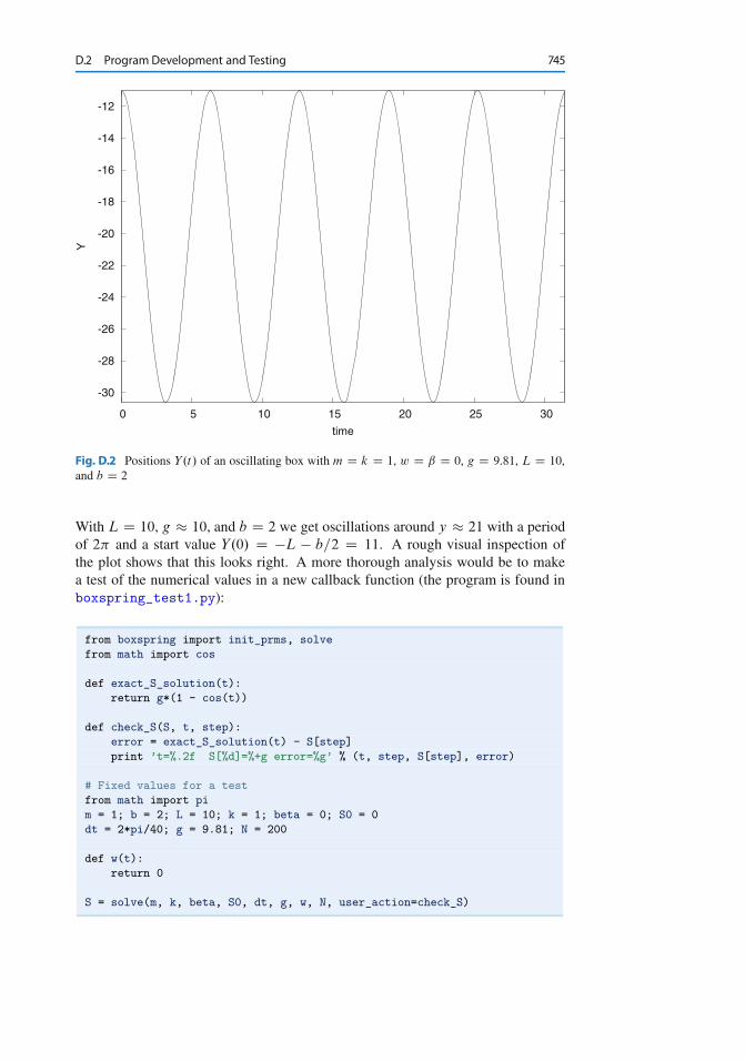
D.2 Program Development and Testing 745
-30
-28
-26
-24
-22
-20
-18
-16
-14
-12
0 5 10 15 20 25 30
Y
time
Fig. D.2 Positions Y.t/ of an oscillating box with m D k D 1, w D ˇ D 0, g D 9:81, L D 10,and b D 2
With L D 10, g � 10, and b D 2 we get oscillations around y � 21 with a periodof 2� and a start value Y.0/ D �L � b=2 D 11. A rough visual inspection ofthe plot shows that this looks right. A more thorough analysis would be to makea test of the numerical values in a new callback function (the program is found inboxspring_test1.py):
from boxspring import init_prms, solve
from math import cos
def exact_S_solution(t):
return g*(1 - cos(t))
def check_S(S, t, step):
error = exact_S_solution(t) - S[step]
print ’t=%.2f S[%d]=%+g error=%g’ % (t, step, S[step], error)
# Fixed values for a test
from math import pi
m = 1; b = 2; L = 10; k = 1; beta = 0; S0 = 0
dt = 2*pi/40; g = 9.81; N = 200
def w(t):
return 0
S = solve(m, k, beta, S0, dt, g, w, N, user_action=check_S)
746 D A Complete Differential Equation Project
The output from this program shows increasing errors with time, up as largevalues as 0.3. The difficulty is to judge whether this is the error one must expectbecause the program computes an approximate solution, or if this error points toa bug in the program – or a wrong mathematical formula.
From these sessions on program testing you will probably realize that verificationof mathematical software is challenging. In particular, the design of the test prob-lems and the interpretation of the numerical output require quite some experiencewith the interplay between physics (or another application discipline), mathematics,and programming.
D.3 Visualization
The purpose of this section is to add graphics to the oscillating system applicationdeveloped in Sect. D.2. Recall that the function solve solves the problem andreturns a list S with indices from 0 to N. Our aim is to plot this list and variousphysical quantities computed from it.
D.3.1 Simultaneous Computation and Plotting
The solve function makes a call back to the user’s code through a callback function(the user_action argument to solve) at each time level. The callback functionhas three arguments: S, the time, and the current time step number. Now we wantthe callback function to plot the position Y.t/ of the box during the computations.In principle this is easy, but S is longer than we want to plot, because S is allocatedfor the whole time simulation while the user_action function is called at timelevels where only the indices in S up to the current time level have been computed(the rest of the elements in S are zero). We must therefore use a sublist of S, fromtime zero and up to the current time. The callback function we send to solve as theuser_action argument can then be written like this:
def plot_S(S, t, step):
if step == 0: # nothing to plot yet
return None
tcoor = linspace(0, t, step+1)
S = array(S[:len(tcoor)])
Y = w(tcoor) - L - S - b/2.
plot(tcoor, Y)
Note that L, dt, b, and w must be global variables in the user’s main program.The major problem with the plot_S function shown is that the w(tcoor) eval-
uation does not work. The reason is that w is a StringFunction object, andaccording to Sect. 5.5.1, StringFunction objects do not work with array argu-ments unless we call their vectorize function once. We therefore need to do a
w.vectorize(globals())
D.3 Visualization 747
before calling solve (which calls plot_S repeatedly). Here is the main programwith this important statement:
from boxspring import init_prms, solve
from scitools.std import *
# Default values
m = 1; b = 2; L = 10; k = 1; beta = 0; S0 = 1;
dt = 2*pi/40; g = 9.81; w_formula = ’0’; N = 200;
m, b, L, k, beta, S0, dt, g, w, N = \
init_prms(m, b, L, k, beta, S0, dt, g, w_formula, N)
w.vectorize(globals())
S = solve(m, k, beta, S0, dt, g, w, N, user_action=plot_S)
Now the plot_S function works fine. You can try the program out by running
Terminal
boxspring_plot_v1.py
Fixing axes Both the t and the y axes adapt to the solution array in every plot. Theadaptation of the y is okay since it is difficult to predict the future minimum andmaximum values of the solution, and hence it is most natural to just adapt the y
axis to the computed Y points so far in the simulation. However, the t axis shouldbe fixed throughout the simulation, and this is easy since we know the start and endtimes. The end time is T D N�t and a relevant plot command becomes
plot(tcoor, Y,
axis=[0, N*dt, min(Y), max(Y)],
xlabel=’time’, ylabel=’Y’)
At the end of the simulation it can be nice to make a hardcopy of the last plotcommand performed in the plot_S function. We then just call
savefig(’tmp_Y.pdf’)
after the solve function is finished.In the beginning of the simulation it is convenient to skip plotting for a number
of steps until there are some interesting points to visualize and to use for computingthe axis extent. We also suggest to apply the recipe at the end of Sect. 5.5.1 tovectorize w. More precisely, we use w.vectorize in general, but turn to numpy’svectorize feature only if the string formula contains an inline if-else test (toavoid requiring users to use where to vectorize the string expressions). One reasonfor paying attention to if-else tests in the w formula is that sudden movements ofthe plate are of interest, and this gives rise to step functions and strings like ’1 ift>0 else 0’. A main program with all these features is listed next.
748 D A Complete Differential Equation Project
from boxspring import init_prms, solve
from scitools.std import *
def plot_S(S, t, step):
first_plot_step = 10 # skip the first steps
if step < first_plot_step:
return
tcoor = linspace(0, t, step+1) # t = dt*step
S = array(S[:len(tcoor)])
Y = w(tcoor) - L - S - b/2.0 # (w, L, b are global vars.)
plot(tcoor, Y,
axis=[0, N*dt, min(Y), max(Y)],
xlabel=’time’, ylabel=’Y’)
# Default values
m = 1; b = 2; L = 10; k = 1; beta = 0; S0 = 1
dt = 2*pi/40; g = 9.81; w_formula = ’0’; N = 200
m, b, L, k, beta, S0, dt, g, w, N = \
init_prms(m, b, L, k, beta, S0, dt, g, w_formula, N)
# Vectorize the StringFunction w
w_formula = str(w) # keep this to see if w=0 later
if ’ else ’ in w_formula:
w = vectorize(w) # general vectorization
else:
w.vectorize(globals()) # more efficient (when no if)
S = solve(m, k, beta, S0, dt, g, w, N, user_action=plot_S)
# First make a hardcopy of the the last plot of Y
savefig(’tmp_Y.pdf’)
D.3.2 Some Applications
What if we suddenly, right after t D 0, move the plate upward from y D 0 toy D 1? This will set the system in motion, and the task is to find out what themotion looks like.
There is no initial stretch in the spring, so the initial condition becomes S0 D 0.We turn off gravity for simplicity and try a w D 1 function since the plate has theposition y D w D 1 for t > 0:
Terminal
boxspring_plot.py --w ’1’ --S 0 --g 0
Nothing happens. The reason is that we specify w.t/ D 1, but in the equation onlyd 2w=dt2 has an effect and this quantity is zero. What we need to specify is a stepfunction: w D 0 for t � 0 and w D 1 for t > 0. In Python such a function can
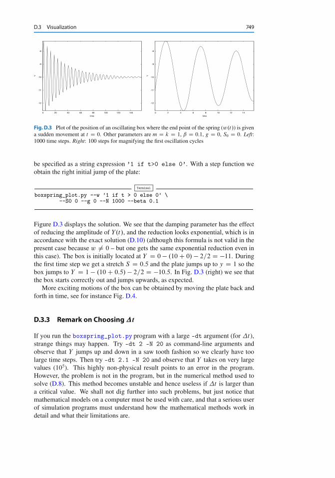
D.3 Visualization 749
-12
-11
-10
-9
-8
0 20 40 60 80 100 120 140
Y
time
-12
-11
-10
-9
-8
0 2 4 6 8 10 12 14
Y
time
Fig. D.3 Plot of the position of an oscillating box where the end point of the spring (w.t/) is givena sudden movement at t D 0. Other parameters are m D k D 1, ˇ D 0:1, g D 0, S0 D 0. Left:1000 time steps. Right: 100 steps for magnifying the first oscillation cycles
be specified as a string expression ’1 if t>0 else 0’. With a step function weobtain the right initial jump of the plate:
Terminal
boxspring_plot.py --w ’1 if t > 0 else 0’ \--S0 0 --g 0 --N 1000 --beta 0.1
Figure D.3 displays the solution. We see that the damping parameter has the effectof reducing the amplitude of Y.t/, and the reduction looks exponential, which is inaccordance with the exact solution (D.10) (although this formula is not valid in thepresent case because w ¤ 0 – but one gets the same exponential reduction even inthis case). The box is initially located at Y D 0 � .10 C 0/ � 2=2 D �11. Duringthe first time step we get a stretch S D 0:5 and the plate jumps up to y D 1 so thebox jumps to Y D 1 � .10 C 0:5/ � 2=2 D �10:5. In Fig. D.3 (right) we see thatthe box starts correctly out and jumps upwards, as expected.
More exciting motions of the box can be obtained by moving the plate back andforth in time, see for instance Fig. D.4.
D.3.3 Remark on Choosing�t
If you run the boxspring_plot.py program with a large –dt argument (for �t),strange things may happen. Try –dt 2 –N 20 as command-line arguments andobserve that Y jumps up and down in a saw tooth fashion so we clearly have toolarge time steps. Then try –dt 2.1 –N 20 and observe that Y takes on very largevalues (105). This highly non-physical result points to an error in the program.However, the problem is not in the program, but in the numerical method used tosolve (D.8). This method becomes unstable and hence useless if �t is larger thana critical value. We shall not dig further into such problems, but just notice thatmathematical models on a computer must be used with care, and that a serious userof simulation programs must understand how the mathematical methods work indetail and what their limitations are.
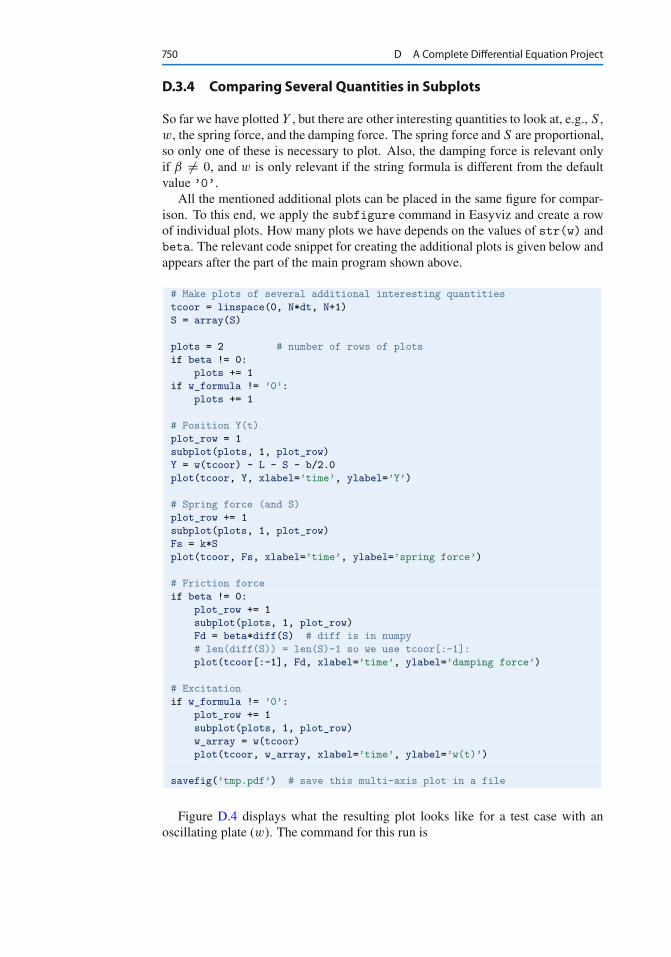
750 D A Complete Differential Equation Project
D.3.4 Comparing Several Quantities in Subplots
So far we have plotted Y , but there are other interesting quantities to look at, e.g., S ,w, the spring force, and the damping force. The spring force and S are proportional,so only one of these is necessary to plot. Also, the damping force is relevant onlyif ˇ ¤ 0, and w is only relevant if the string formula is different from the defaultvalue ’0’.
All the mentioned additional plots can be placed in the same figure for compar-ison. To this end, we apply the subfigure command in Easyviz and create a rowof individual plots. How many plots we have depends on the values of str(w) andbeta. The relevant code snippet for creating the additional plots is given below andappears after the part of the main program shown above.
# Make plots of several additional interesting quantities
tcoor = linspace(0, N*dt, N+1)
S = array(S)
plots = 2 # number of rows of plots
if beta != 0:
plots += 1
if w_formula != ’0’:
plots += 1
# Position Y(t)
plot_row = 1
subplot(plots, 1, plot_row)
Y = w(tcoor) - L - S - b/2.0
plot(tcoor, Y, xlabel=’time’, ylabel=’Y’)
# Spring force (and S)
plot_row += 1
subplot(plots, 1, plot_row)
Fs = k*S
plot(tcoor, Fs, xlabel=’time’, ylabel=’spring force’)
# Friction force
if beta != 0:
plot_row += 1
subplot(plots, 1, plot_row)
Fd = beta*diff(S) # diff is in numpy
# len(diff(S)) = len(S)-1 so we use tcoor[:-1]:
plot(tcoor[:-1], Fd, xlabel=’time’, ylabel=’damping force’)
# Excitation
if w_formula != ’0’:
plot_row += 1
subplot(plots, 1, plot_row)
w_array = w(tcoor)
plot(tcoor, w_array, xlabel=’time’, ylabel=’w(t)’)
savefig(’tmp.pdf’) # save this multi-axis plot in a file
Figure D.4 displays what the resulting plot looks like for a test case with anoscillating plate (w). The command for this run is
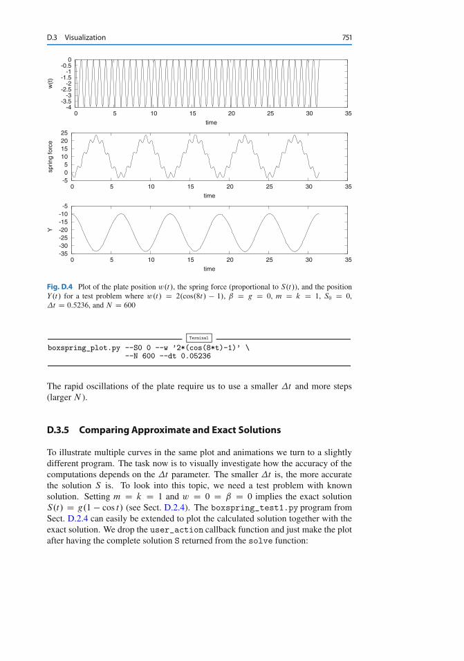
D.3 Visualization 751
-35-30-25-20-15-10-5
0 5 10 15 20 25 30 35
Y
time
-5 0 5
10 15 20 25
0 5 10 15 20 25 30 35
sprin
g fo
rce
time
-4-3.5
-3-2.5
-2-1.5
-1-0.5
0
0 5 10 15 20 25 30 35
w(t
)
time
Fig. D.4 Plot of the plate position w.t/, the spring force (proportional to S.t/), and the positionY.t/ for a test problem where w.t/ D 2.cos.8t/ � 1/, ˇ D g D 0, m D k D 1, S0 D 0,�t D 0:5236, and N D 600
Terminal
boxspring_plot.py --S0 0 --w ’2*(cos(8*t)-1)’ \--N 600 --dt 0.05236
The rapid oscillations of the plate require us to use a smaller �t and more steps(larger N ).
D.3.5 Comparing Approximate and Exact Solutions
To illustrate multiple curves in the same plot and animations we turn to a slightlydifferent program. The task now is to visually investigate how the accuracy of thecomputations depends on the �t parameter. The smaller �t is, the more accuratethe solution S is. To look into this topic, we need a test problem with knownsolution. Setting m D k D 1 and w D 0 D ˇ D 0 implies the exact solutionS.t/ D g.1 � cos t/ (see Sect. D.2.4). The boxspring_test1.py program fromSect. D.2.4 can easily be extended to plot the calculated solution together with theexact solution. We drop the user_action callback function and just make the plotafter having the complete solution S returned from the solve function:
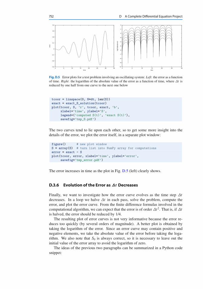
752 D A Complete Differential Equation Project
-0.3
-0.2
-0.1
0
0.1
0.2
0.3
0.4
0 5 10 15 20 25 30 35
erro
r
time
-10
-9
-8
-7
-6
-5
-4
-3
-2
-1
0
0 5 10 15 20 25 30
log1
0(ab
s(er
ror)
)
time
Fig.D.5 Error plots for a test problem involving an oscillating system: Left: the error as a functionof time. Right: the logarithm of the absolute value of the error as a function of time, where �t isreduced by one half from one curve to the next one below
tcoor = linspace(0, N*dt, len(S))
exact = exact_S_solution(tcoor)
plot(tcoor, S, ’r’, tcoor, exact, ’b’,
xlabel=’time’, ylabel=’S’,
legend=(’computed S(t)’, ’exact S(t)’),
savefig=’tmp_S.pdf’)
The two curves tend to lie upon each other, so to get some more insight into thedetails of the error, we plot the error itself, in a separate plot window:
figure() # new plot window
S = array(S) # turn list into NumPy array for computations
error = exact - S
plot(tcoor, error, xlabel=’time’, ylabel=’error’,
savefig=’tmp_error.pdf’)
The error increases in time as the plot in Fig. D.5 (left) clearly shows.
D.3.6 Evolution of the Error as �t Decreases
Finally, we want to investigate how the error curve evolves as the time step �t
decreases. In a loop we halve �t in each pass, solve the problem, compute theerror, and plot the error curve. From the finite difference formulas involved in thecomputational algorithm, we can expect that the error is of order �t2. That is, if �t
is halved, the error should be reduced by 1/4.The resulting plot of error curves is not very informative because the error re-
duces too quickly (by several orders of magnitude). A better plot is obtained bytaking the logarithm of the error. Since an error curve may contain positive andnegative elements, we take the absolute value of the error before taking the loga-rithm. We also note that S0 is always correct, so it is necessary to leave out theinitial value of the error array to avoid the logarithm of zero.
The ideas of the previous two paragraphs can be summarized in a Python codesnippet:
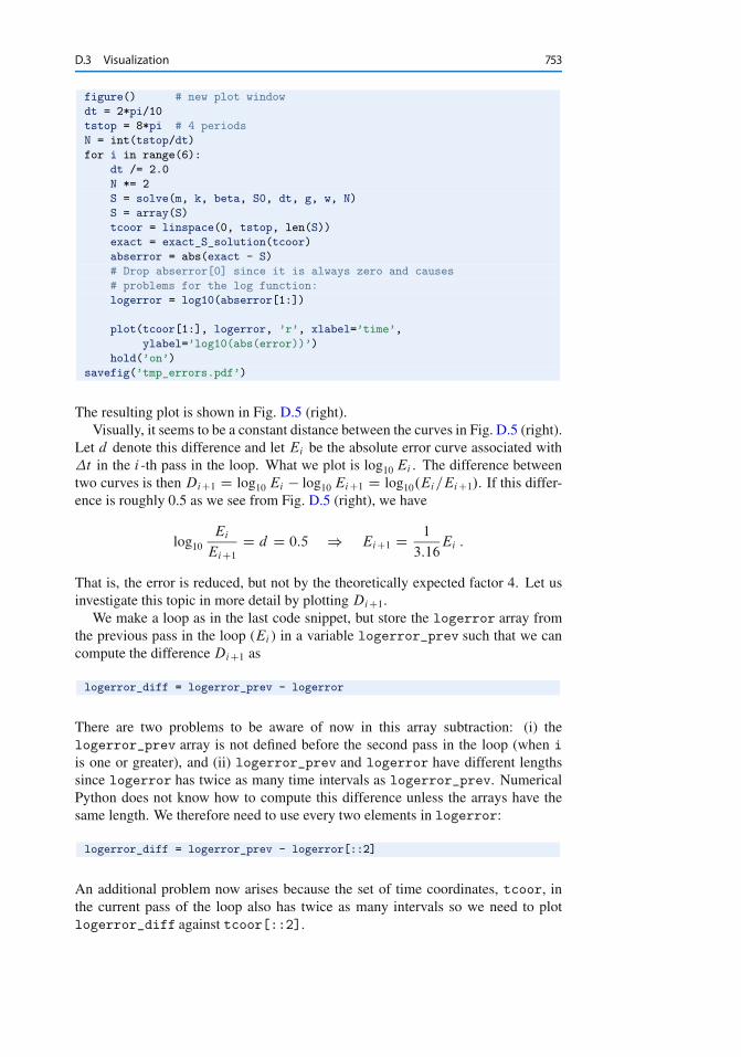
D.3 Visualization 753
figure() # new plot window
dt = 2*pi/10
tstop = 8*pi # 4 periods
N = int(tstop/dt)
for i in range(6):
dt /= 2.0
N *= 2
S = solve(m, k, beta, S0, dt, g, w, N)
S = array(S)
tcoor = linspace(0, tstop, len(S))
exact = exact_S_solution(tcoor)
abserror = abs(exact - S)
# Drop abserror[0] since it is always zero and causes
# problems for the log function:
logerror = log10(abserror[1:])
plot(tcoor[1:], logerror, ’r’, xlabel=’time’,
ylabel=’log10(abs(error))’)
hold(’on’)
savefig(’tmp_errors.pdf’)
The resulting plot is shown in Fig. D.5 (right).Visually, it seems to be a constant distance between the curves in Fig. D.5 (right).
Let d denote this difference and let Ei be the absolute error curve associated with�t in the i-th pass in the loop. What we plot is log10 Ei . The difference betweentwo curves is then DiC1 D log10 Ei � log10 EiC1 D log10.Ei =EiC1/. If this differ-ence is roughly 0.5 as we see from Fig. D.5 (right), we have
log10
Ei
EiC1
D d D 0:5 ) EiC1 D 1
3:16Ei :
That is, the error is reduced, but not by the theoretically expected factor 4. Let usinvestigate this topic in more detail by plotting DiC1.
We make a loop as in the last code snippet, but store the logerror array fromthe previous pass in the loop (Ei ) in a variable logerror_prev such that we cancompute the difference DiC1 as
logerror_diff = logerror_prev - logerror
There are two problems to be aware of now in this array subtraction: (i) thelogerror_prev array is not defined before the second pass in the loop (when iis one or greater), and (ii) logerror_prev and logerror have different lengthssince logerror has twice as many time intervals as logerror_prev. NumericalPython does not know how to compute this difference unless the arrays have thesame length. We therefore need to use every two elements in logerror:
logerror_diff = logerror_prev - logerror[::2]
An additional problem now arises because the set of time coordinates, tcoor, inthe current pass of the loop also has twice as many intervals so we need to plotlogerror_diff against tcoor[::2].
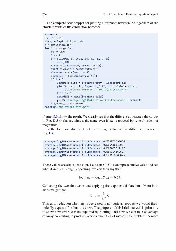
754 D A Complete Differential Equation Project
The complete code snippet for plotting differences between the logarithm of theabsolute value of the errors now becomes
figure()
dt = 2*pi/10
tstop = 8*pi # 4 periods
N = int(tstop/dt)
for i in range(6):
dt /= 2.0
N *= 2
S = solve(m, k, beta, S0, dt, g, w, N)
S = array(S)
tcoor = linspace(0, tstop, len(S))
exact = exact_S_solution(tcoor)
abserror = abs(exact - S)
logerror = log10(abserror[1:])
if i > 0:
logerror_diff = logerror_prev - logerror[::2]
plot(tcoor[1::2], logerror_diff, ’r’, xlabel=’time’,
ylabel=’difference in log10(abs(error))’)
hold(’on’)
meandiff = mean(logerror_diff)
print ’average log10(abs(error)) difference:’, meandiff
logerror_prev = logerror
savefig(’tmp_errors_diff.pdf’)
Figure D.6 shows the result. We clearly see that the differences between the curvesin Fig. D.5 (right) are almost the same even if �t is reduced by several orders ofmagnitude.
In the loop we also print out the average value of the difference curves inFig. D.6:
average log10(abs(error)) difference: 0.558702094666
average log10(abs(error)) difference: 0.56541814902
average log10(abs(error)) difference: 0.576489014172
average log10(abs(error)) difference: 0.585704362507
average log10(abs(error)) difference: 0.592109360025
These values are almost constant. Let us use 0.57 as an representative value and seewhat it implies. Roughly speaking, we can then say that
log10 Ei � log10 EiC1 D 0:57 :
Collecting the two first terms and applying the exponential function 10x on bothsides we get that
EiC1 D 1
3:7Ei :
This error reduction when �t is decreased is not quite as good as we would theo-retically expect (1/4), but it is close. The purpose of this brief analysis is primarilyto show how errors can be explored by plotting, and how we can take advantageof array computing to produce various quantities of interest in a problem. A more
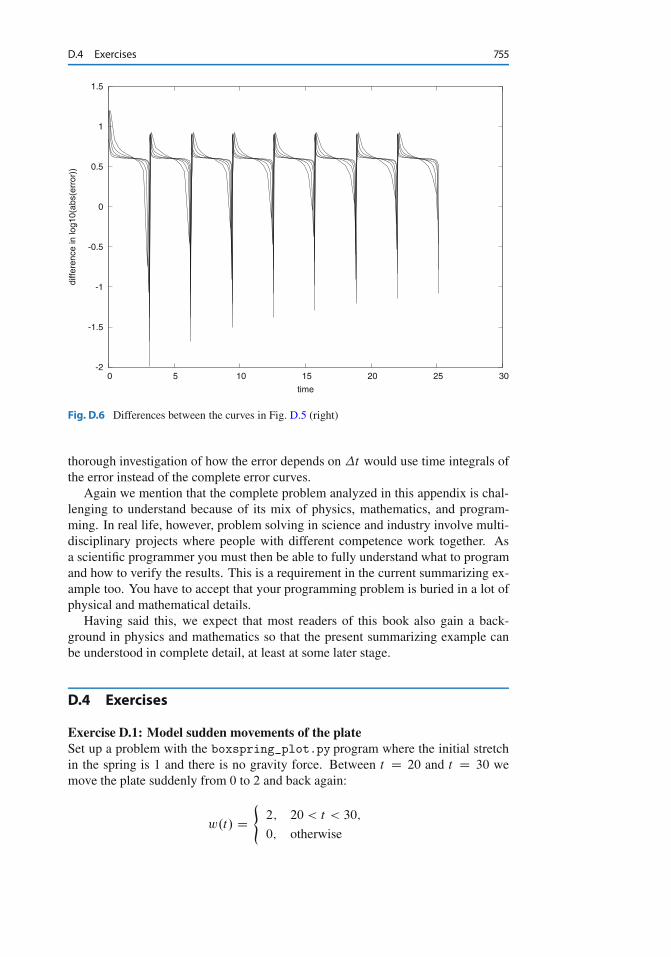
D.4 Exercises 755
-2
-1.5
-1
-0.5
0
0.5
1
1.5
0 5 10 15 20 25 30
diffe
renc
e in
log1
0(ab
s(er
ror)
)
time
Fig. D.6 Differences between the curves in Fig. D.5 (right)
thorough investigation of how the error depends on �t would use time integrals ofthe error instead of the complete error curves.
Again we mention that the complete problem analyzed in this appendix is chal-lenging to understand because of its mix of physics, mathematics, and program-ming. In real life, however, problem solving in science and industry involve multi-disciplinary projects where people with different competence work together. Asa scientific programmer you must then be able to fully understand what to programand how to verify the results. This is a requirement in the current summarizing ex-ample too. You have to accept that your programming problem is buried in a lot ofphysical and mathematical details.
Having said this, we expect that most readers of this book also gain a back-ground in physics and mathematics so that the present summarizing example canbe understood in complete detail, at least at some later stage.
D.4 Exercises
Exercise D.1: Model sudden movements of the plateSet up a problem with the boxspring_plot.py program where the initial stretchin the spring is 1 and there is no gravity force. Between t D 20 and t D 30 wemove the plate suddenly from 0 to 2 and back again:
w.t/ D(
2; 20 < t < 30;
0; otherwise
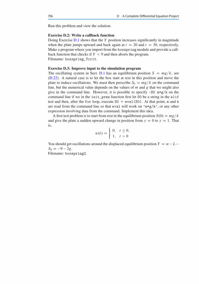
756 D A Complete Differential Equation Project
Run this problem and view the solution.
Exercise D.2: Write a callback functionDoing Exercise D.1 shows that the Y position increases significantly in magnitudewhen the plate jumps upward and back again at t D 20 and t D 30, respectively.Make a programwhere you import from the boxspringmodule and provide a call-back function that checks if Y < 9 and then aborts the program.Filename: boxspring_Ycrit.
Exercise D.3: Improve input to the simulation programThe oscillating system in Sect. D.1 has an equilibrium position S D mg=k, see(D.22). A natural case is to let the box start at rest in this position and move theplate to induce oscillations. We must then prescribe S0 D mg=k on the commandline, but the numerical value depends on the values of m and g that we might alsogive in the command line. However, it is possible to specify –S0 m*g/k on thecommand line if we in the init_prms function first let S0 be a string in the eliftest and then, after the for loop, execute S0 = eval(S0). At that point, m and kare read from the command line so that eval will work on ’m*g/k’, or any otherexpression involving data from the command. Implement this idea.
A first test problem is to start from rest in the equilibrium position S.0/ D mg=k
and give the plate a sudden upward change in position from y D 0 to y D 1. Thatis,
w.t/ D(
0; t � 0;
1; t > 0
You should get oscillations around the displaced equilibrium position Y D w �L�S0 D �9 � 2g.Filename: boxspring2.
EProgramming of Differential Equations
Appendices C and D give a brief introduction to differential equations, with a fo-cus on a few specific equations and programs that are tailored to these equations.The present appendix views differential equations from a more abstract point ofview, which allows us to formulate numerical methods and create general soft-ware that are applicable to a large family of widely different differential equationproblems from mathematics, physics, biology, and finance. More specifically, theabstract view is motivated by the slogan implement once, apply anywhere. Wehave in fact met this principle several places in the book: differentiation (f 00.x/) inSects. 3.1.12 and 7.3.2, integration (
R b
a f .x/dx) in Sects. 3.4.2 and 7.3.3, and rootfinding (f .x/ D 0) in Sect. 4.11.2 and Sect. A.1.10. In all of the referred implemen-tations, we work with a general function f .x/ so that any problem can be solved bythe same piece of code as long as we can define the problem in terms of a functionf .x/. This is an excellent demonstration of the power of mathematics, and thisabstract view of problems in terms of some f .x/ is especially powerful in numer-ical methods and programming. Now we shall formulate differential equations onthe abstract form u0 D f .u; t/ and create software that can solve any equation forwhich the f .u; t/ is given.
Before studying the present appendix, the reader should have some familiaritywith differential equations at the level of Appendix C. Appendix D can also beadvantageous to read, although this is not strictly required. Only fundamental pro-gramming skills regarding loops, lists, arrays, functions, if tests, command-linearguments, and curve plotting are required for the basic function-based material inthis appendix. However, Sects. E.1.7 and E.2.4, as well as many exercises, useclasses to a large extent and hence demand familiarity with the class concept fromChap. 7. The material on object-oriented programming in Sect. E.3 requires goodknowledge of class hierarchies and inheritance from Chap. 9.
All computer codes associated with this appendix is found in src/ode21.
1 http://tinyurl.com/pwyasaa/ode2
757
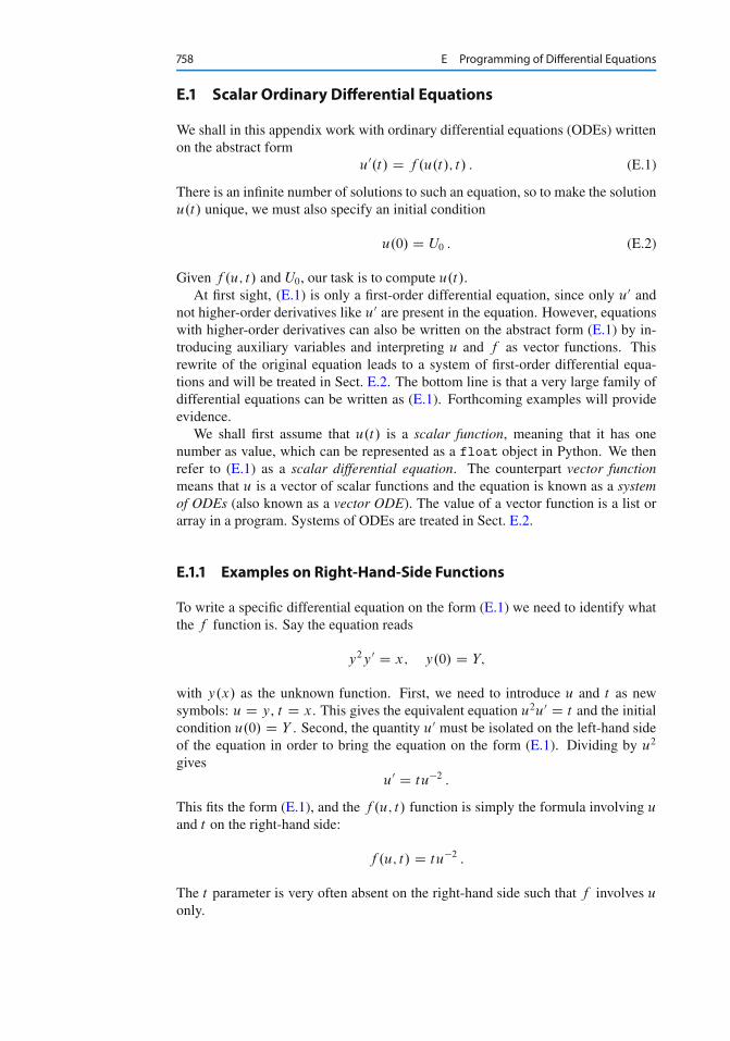
758 E Programming of Differential Equations
E.1 Scalar Ordinary Differential Equations
We shall in this appendix work with ordinary differential equations (ODEs) writtenon the abstract form
u0.t/ D f .u.t/; t/ : (E.1)
There is an infinite number of solutions to such an equation, so to make the solutionu.t/ unique, we must also specify an initial condition
u.0/ D U0 : (E.2)
Given f .u; t/ and U0, our task is to compute u.t/.At first sight, (E.1) is only a first-order differential equation, since only u0 and
not higher-order derivatives like u0 are present in the equation. However, equationswith higher-order derivatives can also be written on the abstract form (E.1) by in-troducing auxiliary variables and interpreting u and f as vector functions. Thisrewrite of the original equation leads to a system of first-order differential equa-tions and will be treated in Sect. E.2. The bottom line is that a very large family ofdifferential equations can be written as (E.1). Forthcoming examples will provideevidence.
We shall first assume that u.t/ is a scalar function, meaning that it has onenumber as value, which can be represented as a float object in Python. We thenrefer to (E.1) as a scalar differential equation. The counterpart vector functionmeans that u is a vector of scalar functions and the equation is known as a systemof ODEs (also known as a vector ODE). The value of a vector function is a list orarray in a program. Systems of ODEs are treated in Sect. E.2.
E.1.1 Examples on Right-Hand-Side Functions
To write a specific differential equation on the form (E.1) we need to identify whatthe f function is. Say the equation reads
y2y0 D x; y.0/ D Y;
with y.x/ as the unknown function. First, we need to introduce u and t as newsymbols: u D y, t D x. This gives the equivalent equation u2u0 D t and the initialcondition u.0/ D Y . Second, the quantity u0 must be isolated on the left-hand sideof the equation in order to bring the equation on the form (E.1). Dividing by u2
givesu0 D tu�2 :
This fits the form (E.1), and the f .u; t/ function is simply the formula involving u
and t on the right-hand side:
f .u; t/ D tu�2 :
The t parameter is very often absent on the right-hand side such that f involves u
only.
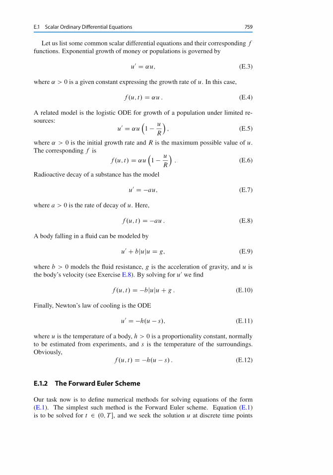
E.1 Scalar Ordinary Differential Equations 759
Let us list some common scalar differential equations and their corresponding f
functions. Exponential growth of money or populations is governed by
u0 D ˛u; (E.3)
where ˛ > 0 is a given constant expressing the growth rate of u. In this case,
f .u; t/ D ˛u : (E.4)
A related model is the logistic ODE for growth of a population under limited re-sources:
u0 D ˛u�1 � u
R
�; (E.5)
where ˛ > 0 is the initial growth rate and R is the maximum possible value of u.The corresponding f is
f .u; t/ D ˛u�1 � u
R
�: (E.6)
Radioactive decay of a substance has the model
u0 D �au; (E.7)
where a > 0 is the rate of decay of u. Here,
f .u; t/ D �au : (E.8)
A body falling in a fluid can be modeled by
u0 C bjuju D g; (E.9)
where b > 0 models the fluid resistance, g is the acceleration of gravity, and u isthe body’s velocity (see Exercise E.8). By solving for u0 we find
f .u; t/ D �bjuju C g : (E.10)
Finally, Newton’s law of cooling is the ODE
u0 D �h.u � s/; (E.11)
where u is the temperature of a body, h > 0 is a proportionality constant, normallyto be estimated from experiments, and s is the temperature of the surroundings.Obviously,
f .u; t/ D �h.u � s/ : (E.12)
E.1.2 The Forward Euler Scheme
Our task now is to define numerical methods for solving equations of the form(E.1). The simplest such method is the Forward Euler scheme. Equation (E.1)is to be solved for t 2 .0; T �, and we seek the solution u at discrete time points
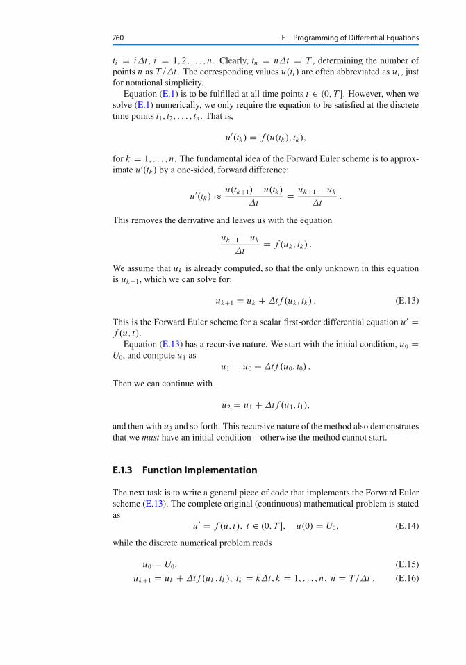
760 E Programming of Differential Equations
ti D i�t , i D 1; 2; : : : ; n. Clearly, tn D n�t D T , determining the number ofpoints n as T=�t . The corresponding values u.ti / are often abbreviated as ui , justfor notational simplicity.
Equation (E.1) is to be fulfilled at all time points t 2 .0; T �. However, when wesolve (E.1) numerically, we only require the equation to be satisfied at the discretetime points t1; t2; : : : ; tn. That is,
u0.tk/ D f .u.tk/; tk/;
for k D 1; : : : ; n. The fundamental idea of the Forward Euler scheme is to approx-imate u0.tk/ by a one-sided, forward difference:
u0.tk/ � u.tkC1/ � u.tk/
�tD ukC1 � uk
�t:
This removes the derivative and leaves us with the equation
ukC1 � uk
�tD f .uk; tk/ :
We assume that uk is already computed, so that the only unknown in this equationis ukC1, which we can solve for:
ukC1 D uk C �tf .uk; tk/ : (E.13)
This is the Forward Euler scheme for a scalar first-order differential equation u0 Df .u; t/.
Equation (E.13) has a recursive nature. We start with the initial condition, u0 DU0, and compute u1 as
u1 D u0 C �tf .u0; t0/ :
Then we can continue with
u2 D u1 C �tf .u1; t1/;
and then with u3 and so forth. This recursive nature of the method also demonstratesthat we must have an initial condition – otherwise the method cannot start.
E.1.3 Function Implementation
The next task is to write a general piece of code that implements the Forward Eulerscheme (E.13). The complete original (continuous) mathematical problem is statedas
u0 D f .u; t/; t 2 .0; T �; u.0/ D U0; (E.14)
while the discrete numerical problem reads
u0 D U0; (E.15)
ukC1 D uk C �tf .uk; tk/; tk D k�t; k D 1; : : : ; n; n D T=�t : (E.16)
E.1 Scalar Ordinary Differential Equations 761
We see that the input data to the numerical problem consist of f , U0, T , and �t orn. The output consists of u1; u2; : : : ; un and the corresponding set of time pointst1; t2; : : : ; tn.
Let us implement the Forward Euler method in a function ForwardEuler thattakes f , U0, T , and n as input, and that returns u0; : : : ; un and t0; : : : ; tn:
import numpy as np
def ForwardEuler(f, U0, T, n):
"""Solve u’=f(u,t), u(0)=U0, with n steps until t=T."""
t = np.zeros(n+1)
u = np.zeros(n+1) # u[k] is the solution at time t[k]
u[0] = U0
t[0] = 0
dt = T/float(n)
for k in range(n):
t[k+1] = t[k] + dt
u[k+1] = u[k] + dt*f(u[k], t[k])
return u, t
Note the close correspondence between the implementation and the mathemati-cal specification of the problem to be solved. The argument f to the ForwardEulerfunction must be a Python function f(u, t) implementing the f .u; t/ function inthe differential equation. In fact, f is the definition of the equation to be solved. Forexample, we may solve u0 D u for t 2 .0; 3/, with u.0/ D 1, and �t D 0:1 by thefollowing code utilizing the ForwardEuler function:
def f(u, t):
return u
u, t = ForwardEuler(f, U0=1, T=4, n=20)
With the u and t arrays we can easily plot the solution or perform data analysison the numbers.
E.1.4 Verifying the Implementation
Visual comparison Many computational scientists and engineers look at a plot tosee if a numerical and exact solution are sufficiently close, and if so, they concludethat the program works. This is, however, not a very reliable test. Consider a firsttry at running ForwardEuler(f, U0=1, T=4, n=10), which gives the plot to theleft in Fig. E.1. The discrepancy between the solutions is large, and the viewer maybe uncertain whether the program works correctly or not. Running n=20 shouldgive a better solution, depicted to the right in Fig. E.1, but is the improvement goodenough? Increasing n drives the numerical curve closer to the exact one. Thisbrings evidence that the program is correct, but there could potentially be errors inthe code that makes the curves further apart than what is implied by the numericalapproximations alone. We cannot know if such a problem exists.
762 E Programming of Differential Equations
0
10
20
30
40
50
60
0 0.5 1 1.5 2 2.5 3 3.5 4
u
t
Solution of the ODE u’=u, u(0)=1
numericalexact
0
10
20
30
40
50
60
0 0.5 1 1.5 2 2.5 3 3.5 4
u
t
Solution of the ODE u’=u, u(0)=1
numericalexact
Fig. E.1 Comparison of numerical exact solution for 10 intervals (left) and 20 (intervals)
Comparing with hand calculations A more rigorous way of verifying the imple-mentation builds on a simple principle: we run the algorithm by hand a few timesand compare the results with those in the program. For most practical purposes, itsuffices to compute u1 and u2 by hand:
u1 D 1 C 0:1 � 1 D 1:1; u2 D 1:1 C 0:1 � 1:1 D 1:21 :
These values are to be compared with the numbers produced by the code. A correctprogram will lead to deviations that are zero (to machine precision). Any such testshould be wrapped in a proper test function such that it can easily be repeated later.Here, it means we make a function
def test_ForwardEuler_against_hand_calculations():
"""Verify ForwardEuler against hand calc. for 3 time steps."""
u, t = ForwardEuler(f, U0=1, T=0.2, n=2)
exact = np.array([1, 1.1, 1.21]) # hand calculations
error = np.abs(exact - u).max()
success = error < 1E-14
assert success, ’|exact - u| = %g != 0’ % error
The test function is written in a way that makes it trivial to integrate it in thenose testing framework, see Sect. H.9 and the brief examples in Sects. 3.3.3, 3.4.2,and 4.9.4. This means that the name starts with test_, there are no function argu-ments, and the check for passing the test is done with assert success. The testfails if the boolean variable success is False. The string after assert successis a message that will be written out if the test fails. The error measure is most con-veniently a scalar number, which here is taken as the absolute value of the largestdeviation between the exact and the numerical solution. Although we expect the er-ror measure to be zero, we are prepared for rounding errors and must use a tolerancewhen testing if the test has passed.
Comparing with an exact numerical solution Another effective way to verifythe code, is to find a problem that can be solved exactly by the numerical methodwe use. That is, we seek a problem where we do not have to deal with numericalapproximation errors when comparing the exact solution with the one produced bythe program. It turns out that if the solution u.t/ is linear in t , the Forward Euler
E.1 Scalar Ordinary Differential Equations 763
method will reproduce this solution exactly. Therefore, we choose u.t/ D at C U0,with (e.g.) a D 0:2 and U0 D 3. The corresponding f is the derivative of u, i.e.,f .u; t/ D a. This is obviously a very simple right-hand side without any u or t .However, we can make f more complicated by adding something that is zero, e.g.,some expression with u � .at C U0/, say .u � .at C U0//
4, so that
f .u; t/ D a C .u � .at C U0//4 : (E.17)
We implement our special f and the exact solution in two functions f andu_exact, and compute a scalar measure of the error. As a above, we place thetest inside a test function and make an assertion that the error is sufficiently close tozero:
def test_ForwardEuler_against_linear_solution():
"""Use knowledge of an exact numerical solution for testing."""
def f(u, t):
return 0.2 + (u - u_exact(t))**4
def u_exact(t):
return 0.2*t + 3
u, t = ForwardEuler(f, U0=u_exact(0), T=3, n=5)
u_e = u_exact(t)
error = np.abs(u_e - u).max()
success = error < 1E-14
assert success, ’|exact - u| = %g != 0’ % error
A “silent” execution of the function indicates that the test works.The shown functions are collected in a file ForwardEuler_func.py.
E.1.5 From Discrete to Continuous Solution
The numerical solution of an ODE is a discrete function in the sense that we onlyknow the function values u0; u1; ldots; uN at some discrete points t0; t1; : : : ; tN intime. What if we want to know u between two computed points? For example,what is u between ti and tiC1, say at the midpoint t D ti C 1
2�t? One can use
interpolation techniques to find this value u. The simplest interpolation techniqueis to assume that u varies linearly on each time interval. On the interval Œti ; tiC1� thelinear variation of u becomes
u.t/ D ui C uiC1 � ui
tiC1 � ti.t � ti / :
We can then evaluate, e.g., u.ti C 12�t/ from this formula and show that it becomes
.ui C uiC1/=2.The function scitools.std.wrap2callable can automatically convert a dis-
crete function to a continuous function:
from scitools.std import wrap2callable
u_cont = wrap2callable((t, u))
764 E Programming of Differential Equations
From the arrays t and u, wrap2callable constructs a continuous function basedon linear interpolation. The result u_cont is a Python function that we can evaluatefor any value of its argument t:
dt = t[i+1] - t[i]
t = t[i] + 0.5*dt
value = u_cont(t)
In general, the wrap2callable function is handy when you have computedsome discrete function and you want to evaluate this discrete function at any point.
E.1.6 Switching Numerical Method
There are numerous alternative numerical methods for solving (E.13). One of thesimplest is Heun’s method:
u� D uk C �tf .uk; tk/; (E.18)
ukC1 D uk C 1
2�tf .uk; tk/ C 1
2�tf .u�; tkC1/ : (E.19)
This scheme is easily implemented in the ForwardEuler function by replacing theForward Euler formula
u[k+1] = u[k] + dt*f(u[k], t[k])
by (E.18) and (E.19):
u_star = u[k] + dt*f(u[k], t[k])
u[k+1] = u[k] + 0.5*dt*f(u[k], t[k]) + 0.5*dt*f(u_star, t[k+1])
We can, especially if f is expensive to calculate, eliminate a call f(u[k], t[k])by introducing an auxiliary variable:
f_k = f(u[k], t[k])
u_star = u[k] + dt*f_k
u[k+1] = u[k] + 0.5*dt*f_k + 0.5*dt*f(u_star, t[k+1])
E.1.7 Class Implementation
As an alternative to the general ForwardEuler function in Sect. E.1.3, we shall nowimplement the numerical method in a class. This requires, of course, familiaritywith the class concept from Chap. 7.
Class wrapping of a function Let us start with simply wrapping the ForwardEulerfunction in a class ForwardEuler_v1 (the postfix _v1 indicates that this is the very
E.1 Scalar Ordinary Differential Equations 765
first class version). That is, we take the code in the ForwardEuler function anddistribute it among methods in a class.
The constructor can store the input data of the problem and initialize data struc-tures, while a solvemethod can perform the time stepping procedure:
import numpy as np
class ForwardEuler_v1(object):
def __init__(self, f, U0, T, n):
self.f, self.U0, self.T, self.n = f, dt, U0, T, n
self.dt = T/float(n)
self.u = np.zeros(n+1)
self.t = np.zeros(n+1)
def solve(self):
"""Compute solution for 0 <= t <= T."""
self.u[0] = float(self.U0)
self.t[0] = float(0)
for k in range(self.n):
self.k = k
self.t[k+1] = self.t[k] + self.dt
self.u[k+1] = self.advance()
return self.u, self.t
def advance(self):
"""Advance the solution one time step."""
u, dt, f, k, t = \
self.u, self.dt, self.f, self.k, self.t
u_new = u[k] + dt*f(u[k], t[k])
return u_new
Note that we have introduced a third class method, advance, which isolates thenumerical scheme. The motivation is that, by observation, the constructor and thesolve method are completely general as they remain unaltered if we change thenumerical method (at least this is true for a wide class of numerical methods). Theonly difference between various numerical schemes is the updating formula. It istherefore a good programming habit to isolate the updating formula so that anotherscheme can be implemented by just replacing the advancemethod – without touch-ing any other parts of the class.
Also note that we in the advancemethod “strip off” the self prefix by introduc-ing local symbols with exactly the same names as in the mathematical specificationof the numerical method. This is important if we want a visually one-to-one corre-spondence between the mathematics and the computer code.
Application of the class goes as follows, here for the model problem u0 D u,u.0/ D 1:
def f(u, t):
return u
solver = ForwardEuler_v1(f, U0=1, T=3, n=15)
u, t = solver.solve()
766 E Programming of Differential Equations
Switching numerical method Implementing, for example, Heun’s method (E.18)–(E.19) is a matter of replacing the advancemethod by
def advance(self):
"""Advance the solution one time step."""
u, dt, f, k, t = \
self.u, self.dt, self.f, self.k, self.t
u_star = u[k] + dt*f(u[k], t[k])
u_new = u[k] + \
0.5*dt*f(u[k], t[k]) + 0.5*dt*f(u_star, t[k+1])
return u_new
Checking input data is always a good habit, and in the present class the construc-tor may test that the f argument is indeed an object that can be called as a function:
if not callable(f):
raise TypeError(’f is %s, not a function’ % type(f))
Any function f or any instance of a class with a __call__ method will makecallable(f) evaluate to True.
A more flexible class Say we solve u0 D f .u; t/ from t D 0 to t D T1. Wecan continue the solution for t > T1 simply by restarting the whole procedurewith initial conditions at t D T1. Hence, the implementation should allow severalconsequtive solve steps.
Another fact is that the time step �t does not need to be constant. Allowingsmall �t in regions where u changes rapidly and letting �t be larger in areas whereu is slowly varying, is an attractive solution strategy. The Forward Euler methodcan be reformulated for a variable time step size tkC1 � tk :
ukC1 D uk C .tkC1 � tk/f .uk; tk/ : (E.20)
Similarly, Heun’s method and many other methods can be formulated with a vari-able step size simply by replacing �t with tkC1 � tk . It then makes sense forthe user to provide a list or array with time points for which a solution is sought:t0; t1; : : : ; tn. The solvemethod can accept such a set of points.
The mentioned extensions lead to a modified class:
class ForwardEuler(object):
def __init__(self, f):
if not callable(f):
raise TypeError(’f is %s, not a function’ % type(f))
self.f = f
def set_initial_condition(self, U0):
self.U0 = float(U0)
E.1 Scalar Ordinary Differential Equations 767
def solve(self, time_points):
"""Compute u for t values in time_points list."""
self.t = np.asarray(time_points)
self.u = np.zeros(len(time_points))
# Assume self.t[0] corresponds to self.U0
self.u[0] = self.U0
for k in range(len(self.t)-1):
self.k = k
self.u[k+1] = self.advance()
return self.u, self.t
def advance(self):
"""Advance the solution one time step."""
u, f, k, t = self.u, self.f, self.k, self.t
dt = t[k+1] - t[k]
u_new = u[k] + dt*f(u[k], t[k])
return u_new
Usage of the class We must instantiate an instance, call the set_initial_conditionmethod, and then call the solvemethod with a list or array of the timepoints we want to compute u at:
def f(u, t):
"""Right-hand side function for the ODE u’ = u."""
return u
solver = ForwardEuler(f)
solver.set_initial_condition(2.5)
u, t = solver.solve(np.linspace(0, 4, 21))
A simple plot(t, u) command can visualize the solution.
Verification It is natural to perform the same verifications as we did for theForwardEuler function in Sect. E.1.4. First, we test the numerical solution againsthand calculations. The implementation makes use of the same test function, justthe way of calling up the numerical solver is different:
def test_ForwardEuler_against_hand_calculations():
"""Verify ForwardEuler against hand calc. for 2 time steps."""
solver = ForwardEuler(lambda u, t: u)
solver.set_initial_condition(1)
u, t = solver.solve([0, 0.1, 0.2])
exact = np.array([1, 1,1, 1.21]) # hand calculations
error = np.abs(exact - u).max()
assert error < 1E-14, ’|exact - u| = %g != 0’ % error
We have put some efforts into making this test very compact, mainly to demonstratehow Python allows very short, but still readable code. With a lambda function wecan define the right-hand side of the ODE directly in the constructor argument. Thesolvemethod accepts a list, tuple, or array of time points and turns the data into anarray anyway. Instead of a separate boolean variable successwe have inserted thetest inequality directly in the assert statement.
768 E Programming of Differential Equations
The second verification method applies the fact that the Forward Euler schemeis exact for a u that is linear in t . We perform a slightly more complicated test thanin Sect. E.1.4: now we first solve for the points 0; 0:4; 1; 1:2, and then we continuethe solution process for t1 D 1:4 and t2 D 1:5.
def test_ForwardEuler_against_linear_solution():
"""Use knowledge of an exact numerical solution for testing."""
u_exact = lambda t: 0.2*t + 3
solver = ForwardEuler(lambda u, t: 0.2 + (u - u_exact(t))**4)
# Solve for first time interval [0, 1.2]
solver.set_initial_condition(u_exact(0))
u1, t1 = solver.solve([0, 0.4, 1, 1.2])
# Continue with a new time interval [1.2, 1.5]
solver.set_initial_condition(u1[-1])
u2, t2 = solver.solve([1.2, 1.4, 1.5])
# Append u2 to u1 and t2 to t1
u = np.concatenate((u1, u2))
t = np.concatenate((t1, t2))
u_e = u_exact(t)
error = np.abs(u_e - u).max()
assert error < 1E-14, ’|exact - u| = %g != 0’ % error
Making a module It is a well-established programming habit to have class imple-mentations in files that act as Python modules. This means that all code is collectedwithin classes or functions, and that the main program is executed in a test block.Upon import, no test or demonstration code should be executed.
Everything we have made so far is in classes or functions, so the remaining taskto make a module, is to construct the test block.
if __name__ == ’__main__’:
import sys
if len(sys.argv) >= 2 and sys.argv[1] == ’test’:
test_ForwardEuler_v1_against_hand_calculations()
test_ForwardEuler_against_hand_calculations()
test_ForwardEuler_against_linear_solution()
The ForwardEuler_func.py file with functions from Sects. E.1.3 and E.1.4 isin theory a module, but not sufficiently cleaned up. Exercise E.15 encourages youto turn the file into a proper module.
Remark We do not need to call the test functions from the test block, sincewe can let nose run the tests automatically, see Sect. H.9, by nosetests -sForwardEuler.py.
E.1 Scalar Ordinary Differential Equations 769
E.1.8 Logistic Growth via a Function-Based Approach
A more exciting application than the verification problems above is to simulatelogistic growth of a population. The relevant ODE reads
u0.t/ D ˛u.t/
�1 � u.t/
R
�:
The mathematical f .u; t/ function is simply the right-hand side of this ODE. Thecorresponding Python function is
def f(u, t):
return alpha*u*(1 - u/R)
where alpha and R are global variables that correspond to ˛ and R. These must beinitialized before calling the ForwardEuler function (which will call the f(u,t)above):
alpha = 0.2
R = 1.0
from ForwardEuler_func2 import ForwardEuler
u, t = ForwardEuler(f, U0=0.1, T=40, n=400)
We have in this program assumed that Exercise E.15 has been carried out to cleanup the ForwardEuler_func.pyfile such that it becomes a proper module file withthe name ForwardEuler_func2.py.
With u and t computed we can proceed with visualizing the solution (seeFig. E.2):
from matplotlib.pyplot import *
plot(t, u)
xlabel(’t’); ylabel(’u’)
title(’Logistic growth: alpha=%s, R=%g, dt=%g’ %
(alpha, R, t[1]-t[0]))
savefig(’tmp.pdf’); savefig(’tmp.png’)
show()
The complete code appears in the file logistic_func.py.
E.1.9 Logistic Growth via a Class-Based Approach
The task of this section is to redo the implementation of Sect. E.1.8 using a prob-lem class to store the physical parameters and the f .u; t/ function, and using classForwardEuler from Sect. E.1.7 to solve the ODE. Comparison with the code inSect. E.1.8 will then exemplify what the difference between a function-based anda class-based implementation is. There will be two major differences. One is relatedto technical differences between programming with functions and programming
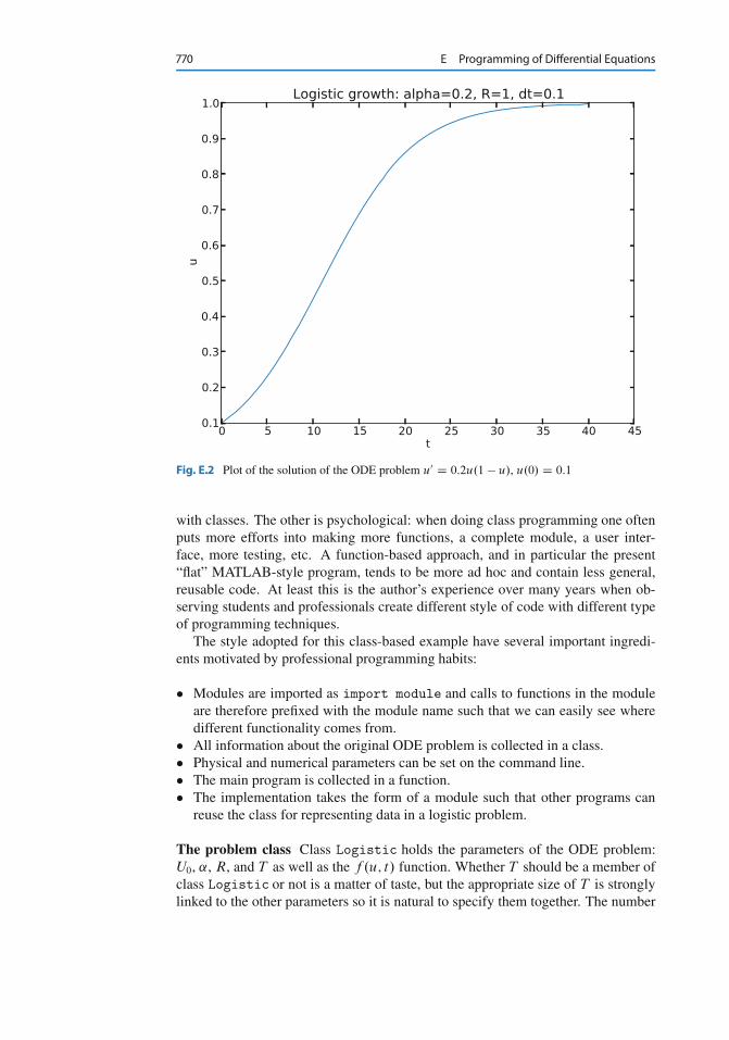
770 E Programming of Differential Equations
Fig. E.2 Plot of the solution of the ODE problem u0 D 0:2u.1 � u/, u.0/ D 0:1
with classes. The other is psychological: when doing class programming one oftenputs more efforts into making more functions, a complete module, a user inter-face, more testing, etc. A function-based approach, and in particular the present“flat” MATLAB-style program, tends to be more ad hoc and contain less general,reusable code. At least this is the author’s experience over many years when ob-serving students and professionals create different style of code with different typeof programming techniques.
The style adopted for this class-based example have several important ingredi-ents motivated by professional programming habits:
Modules are imported as import module and calls to functions in the moduleare therefore prefixed with the module name such that we can easily see wheredifferent functionality comes from.
All information about the original ODE problem is collected in a class. Physical and numerical parameters can be set on the command line. The main program is collected in a function. The implementation takes the form of a module such that other programs can
reuse the class for representing data in a logistic problem.
The problem class Class Logistic holds the parameters of the ODE problem:U0, ˛, R, and T as well as the f .u; t/ function. Whether T should be a member ofclass Logistic or not is a matter of taste, but the appropriate size of T is stronglylinked to the other parameters so it is natural to specify them together. The number
E.1 Scalar Ordinary Differential Equations 771
of time intervals, n, used in the numerical solution method is not a part of classLogistic since it influences the accuracy of the solution, but not the qualitativeproperties of the solution curve as the other parameters do.
The f .u; t/ function is naturally implemented as a __call__method such thatthe problem instance can act as both an instance and a callable function at the sametime. In addition, we include a __str__ for printing out the ODE problem. Thecomplete code for the class looks like
class Logistic(object):
"""Problem class for a logistic ODE."""
def __init__(self, alpha, R, U0, T):
self.alpha, self.R, self.U0, self.T = alpha, float(R), U0, T
def __call__(self, u, t):
"""Return f(u,t) for the logistic ODE."""
return self.alpha*u*(1 - u/self.R)
def __str__(self):
"""Return ODE and initial condition."""
return "u’(t) = %g*u*(1 - u/%g), t in [0, %g]\nu(0)=%g" % \
(self.alpha, self.R, self.T, self.U0)
Getting input from the command line We decide to specify ˛, R, U0, T , and n,in that order, on the command line. A function for converting the command-linearguments into proper Python objects can be
def get_input():
"""Read alpha, R, U0, T, and n from the command line."""
try:
alpha = float(sys.argv[1])
R = float(sys.argv[2])
U0 = float(sys.argv[3])
T = float(sys.argv[4])
n = float(sys.argv[5])
except IndexError:
print ’Usage: %s alpha R U0 T n’ % sys.argv[0]
sys.exit(1)
return alpha, R, U0, T, n
We have used a standard a try-except block to handle potential errors becauseof missing command-line arguments. A more user-friendly alternative would be toallow option-value pairs such that, e.g., T can be set by –T 40 on the commandline, but this requires more programming (with the argparsemodule).
Import statements The import statements necessary for the problem solving pro-cess are written as
import ForwardEuler
import numpy as np
import matplotlib.pyplot as plt
772 E Programming of Differential Equations
The two latter statements with their abbreviations have evolved as a standard inPython code for scientific computing.
Solving the problem The remaining necessary statements for solving a logisticproblem are collected in a function
def logistic():
alpha, R, U0, T, n = get_input()
problem = Logistic(alpha=alpha, R=R, U0=U0)
solver = ForwardEuler.ForwardEuler(problem)
solver.set_initial_condition(problem.U0)
time_points = np.linspace(0, T, n+1)
u, t = solver.solve(time_points)
plt.plot(t, u)
plt.xlabel(’t’); plt.ylabel(’u’)
plt.title(’Logistic growth: alpha=%s, R=%g, dt=%g’
% (problem.alpha, problem.R, t[1]-t[0]))
plt.savefig(’tmp.pdf’); plt.savefig(’tmp.png’)
plt.show()
Making a module Everything we have created is either a class or a function. Theonly remaining task to ensure that the file is a proper module is to place the call tothe “main” function logistic in a test block:
if __name__ == ’__main__’:
logistic()
The complete module is called logistic_class.py.
Pros and cons of the class-based approach If we quickly need to solve an ODEproblem, it is tempting and efficient to go for the function-based code, because itis more direct and much shorter. A class-based module, with a user interface andoften also test functions, usually gives more high-quality code that pays off whenthe software is expected to have a longer life time and will be extended to morecomplicated problems.
A pragmatic approach is to first make a quick function-based code, but refactorthat code to a more reusable and extensible class version with test functions whenyou experience that the code frequently undergo changes. The present simple lo-gistic ODE problem is, in my honest opinion, not complicated enough to defenda class version for practical purposes, but the primary goal here was to use a verysimple mathematical problem for illustrating class programming.
E.2 Systems of Ordinary Differential Equations
The software developed so far in this appendix targets scalar ODEs of the formu0 D f .u; t/ with initial condition u.0/ D U0. Our goal now is to build flexiblesoftware for solving scalar ODEs as well as systems of ODEs. That is, we want thesame code to work both for systems and scalar equations.
E.2 Systems of Ordinary Differential Equations 773
E.2.1 Mathematical Problem
A scalar ODE involves the single equation
u0.t/ D f .u.t/; t/
with a single function u.t/ as unknown, while a system of ODEs involves n scalarODEs and consequently n unknown functions. Let us denote the unknown functionsin the system by u.i/.t/, with i as a counter, i D 0; : : : ; m � 1. The system of n
ODEs can then be written in the following abstract form:
du.0/
dtD f .0/.u.0/; u.1/; : : : ; u.m�1/; t/; (E.21)
:::
du.i/
dtD f .i/.u.0/; u.1/; : : : ; u.m�1/; t/; (E.22)
:::
du.m�1/
dtD f .m�1/.u.0/; u.1/; : : : ; u.m�1/; t/; (E.23)
In addition, we need n initial conditions for the n unknown functions:
u.i/.0/ D U.i/0 ; i D 0; : : : ; m � 1 : (E.24)
Instead of writing out each equation as in (E.21)–(E.23), mathematicians like tocollect the individual functions u.0/; u.1/; : : : ; u.m�1/ in a vector
u D .u.0/; u.1/; : : : ; u.m�1// :
The different right-hand-side functions f .0/; f .1/; : : : ; f .m�1/ in (E.21)–(E.23) canalso be collected in a vector
f D .f .0/; f .1/; : : : ; f .m�1// :
Similarly, we put the initial conditions also in a vector
U0 D .U.0/0 ; U
.1/0 ; : : : ; U
.m�1/0 / :
With the vectors u, f , and U0, we can write the ODE system (E.21)–(E.23) withinitial conditions (E.24) as
u0 D f .u; t/; u.0/ D U0 : (E.25)
This is exactly the same notation as we used for a scalar ODE (!). The power ofmathematics is that abstractions can be generalized so that new problems look likethe familiar ones, and very often methods carry over to the new problems in the newnotation without any changes. This is true for numerical methods for ODEs too.
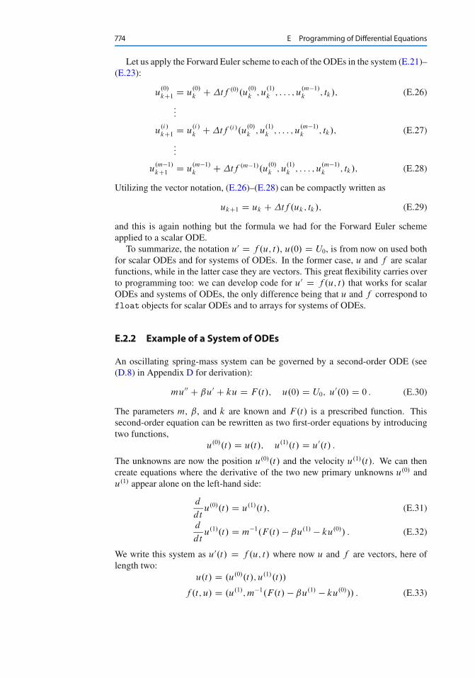
774 E Programming of Differential Equations
Let us apply the Forward Euler scheme to each of the ODEs in the system (E.21)–(E.23):
u.0/
kC1 D u.0/
k C �tf .0/.u.0/
k ; u.1/
k ; : : : ; u.m�1/
k ; tk/; (E.26)
:::
u.i/
kC1 D u.i/
k C �tf .i/.u.0/
k ; u.1/
k ; : : : ; u.m�1/
k ; tk/; (E.27)
:::
u.m�1/
kC1 D u.m�1/
k C �tf .m�1/.u.0/
k ; u.1/
k ; : : : ; u.m�1/
k ; tk/; (E.28)
Utilizing the vector notation, (E.26)–(E.28) can be compactly written as
ukC1 D uk C �tf .uk; tk/; (E.29)
and this is again nothing but the formula we had for the Forward Euler schemeapplied to a scalar ODE.
To summarize, the notation u0 D f .u; t/, u.0/ D U0, is from now on used bothfor scalar ODEs and for systems of ODEs. In the former case, u and f are scalarfunctions, while in the latter case they are vectors. This great flexibility carries overto programming too: we can develop code for u0 D f .u; t/ that works for scalarODEs and systems of ODEs, the only difference being that u and f correspond tofloat objects for scalar ODEs and to arrays for systems of ODEs.
E.2.2 Example of a System of ODEs
An oscillating spring-mass system can be governed by a second-order ODE (see(D.8) in Appendix D for derivation):
mu00 C ˇu0 C ku D F.t/; u.0/ D U0; u0.0/ D 0 : (E.30)
The parameters m, ˇ, and k are known and F.t/ is a prescribed function. Thissecond-order equation can be rewritten as two first-order equations by introducingtwo functions,
u.0/.t/ D u.t/; u.1/.t/ D u0.t/ :
The unknowns are now the position u.0/.t/ and the velocity u.1/.t/. We can thencreate equations where the derivative of the two new primary unknowns u.0/ andu.1/ appear alone on the left-hand side:
d
dtu.0/.t/ D u.1/.t/; (E.31)
d
dtu.1/.t/ D m�1.F.t/ � ˇu.1/ � ku.0// : (E.32)
We write this system as u0.t/ D f .u; t/ where now u and f are vectors, here oflength two:
u.t/ D .u.0/.t/; u.1/.t//
f .t; u/ D .u.1/; m�1.F.t/ � ˇu.1/ � ku.0/// : (E.33)
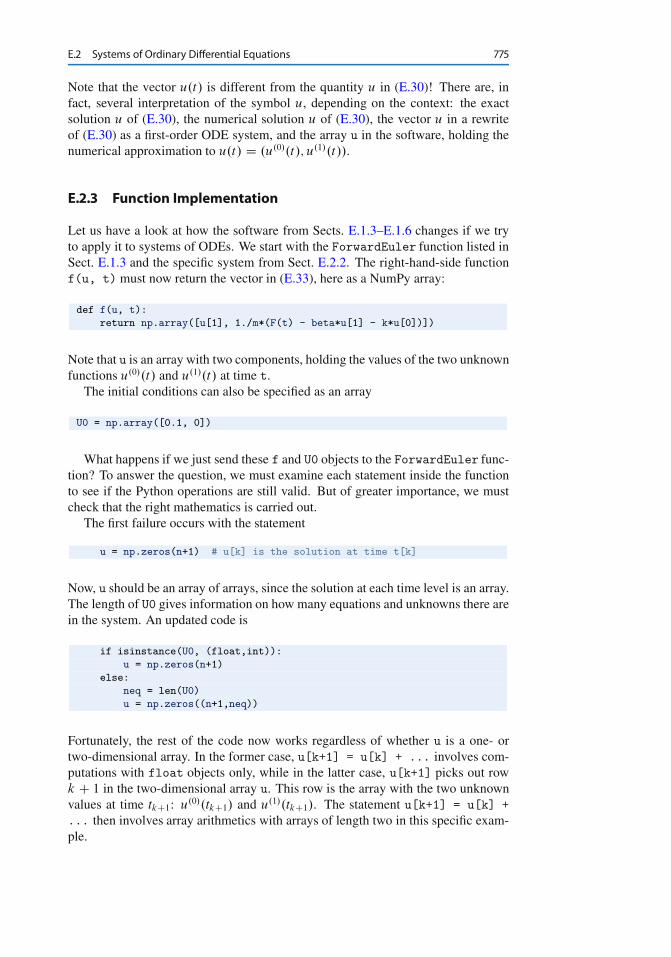
E.2 Systems of Ordinary Differential Equations 775
Note that the vector u.t/ is different from the quantity u in (E.30)! There are, infact, several interpretation of the symbol u, depending on the context: the exactsolution u of (E.30), the numerical solution u of (E.30), the vector u in a rewriteof (E.30) as a first-order ODE system, and the array u in the software, holding thenumerical approximation to u.t/ D .u.0/.t/; u.1/.t//.
E.2.3 Function Implementation
Let us have a look at how the software from Sects. E.1.3–E.1.6 changes if we tryto apply it to systems of ODEs. We start with the ForwardEuler function listed inSect. E.1.3 and the specific system from Sect. E.2.2. The right-hand-side functionf(u, t) must now return the vector in (E.33), here as a NumPy array:
def f(u, t):
return np.array([u[1], 1./m*(F(t) - beta*u[1] - k*u[0])])
Note that u is an array with two components, holding the values of the two unknownfunctions u.0/.t/ and u.1/.t/ at time t.
The initial conditions can also be specified as an array
U0 = np.array([0.1, 0])
What happens if we just send these f and U0 objects to the ForwardEuler func-tion? To answer the question, we must examine each statement inside the functionto see if the Python operations are still valid. But of greater importance, we mustcheck that the right mathematics is carried out.
The first failure occurs with the statement
u = np.zeros(n+1) # u[k] is the solution at time t[k]
Now, u should be an array of arrays, since the solution at each time level is an array.The length of U0 gives information on how many equations and unknowns there arein the system. An updated code is
if isinstance(U0, (float,int)):
u = np.zeros(n+1)
else:
neq = len(U0)
u = np.zeros((n+1,neq))
Fortunately, the rest of the code now works regardless of whether u is a one- ortwo-dimensional array. In the former case, u[k+1] = u[k] + ... involves com-putations with float objects only, while in the latter case, u[k+1] picks out rowk C 1 in the two-dimensional array u. This row is the array with the two unknownvalues at time tkC1: u.0/.tkC1/ and u.1/.tkC1/. The statement u[k+1] = u[k] +... then involves array arithmetics with arrays of length two in this specific exam-ple.
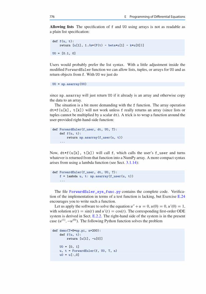
776 E Programming of Differential Equations
Allowing lists The specification of f and U0 using arrays is not as readable asa plain list specification:
def f(u, t):
return [u[1], 1./m*(F(t) - beta*u[1] - k*u[0])]
U0 = [0.1, 0]
Users would probably prefer the list syntax. With a little adjustment inside themodified ForwardEuler function we can allow lists, tuples, or arrays for U0 and asreturn objects from f. With U0 we just do
U0 = np.asarray(U0)
since np.asarray will just return U0 if it already is an array and otherwise copythe data to an array.
The situation is a bit more demanding with the f function. The array operationdt*f(u[k], t[k]) will not work unless f really returns an array (since lists ortuples cannot be multiplied by a scalar dt). A trick is to wrap a function around theuser-provided right-hand-side function:
def ForwardEuler(f_user, dt, U0, T):
def f(u, t):
return np.asarray(f_user(u, t))
...
Now, dt*f(u[k], t[k]) will call f, which calls the user’s f_user and turnswhatever is returned from that function into a NumPy array. A more compact syntaxarises from using a lambda function (see Sect. 3.1.14):
def ForwardEuler(f_user, dt, U0, T):
f = lambda u, t: np.asarray(f_user(u, t))
...
The file ForwardEuler_sys_func.py contains the complete code. Verifica-tion of the implementation in terms of a test function is lacking, but Exercise E.24encourages you to write such a function.
Let us apply the software to solve the equation u00 Cu D 0, u.0/ D 0, u0.0/ D 1,with solution u.t/ D sin.t/ and u0.t/ D cos.t/. The corresponding first-order ODEsystem is derived in Sect. E.2.2. The right-hand side of the system is in the presentcase .u.1/; �u.0//. The following Python function solves the problem
def demo(T=8*np.pi, n=200):
def f(u, t):
return [u[1], -u[0]]
U0 = [0, 1]
u, t = ForwardEuler(f, U0, T, n)
u0 = u[:,0]
E.2 Systems of Ordinary Differential Equations 777
Fig. E.3 Comparison of large (left) and small (right) time step when solving u00 C u D 0 by theForward Euler method
# Plot u0 vs t and compare with exact solution sin(t)
from matplotlib.pyplot import plot, show, savefig, legend
plot(t, u0, ’r-’, t, np.sin(t), ’b--’)
legend([’ForwardEuler, n=%d’ % n, ’exact’], loc=’upper left’)
savefig(’tmp.pdf’)
show()
Storage of the solution of ODE systemsWhen solving systems of ODEs, the computed solution u is a two-dimensionalarray where u[k,i] holds the unknown function number i at time point numberk: u.i/.tk/. Hence, to grab all the values associated with u.0/, we fix i as 0 andlet the k index take on all its legal values: u[:,0]. This slice of the u arrayrefers to the piece of u where the discrete values u.0/.t0/; u.0/.t1/; : : : ; u.0/.tn/
are stored. The remaining part of u, u[:,1], holds all the discrete values of thecomputed u0.t/.
From visualizing the solution, see Fig. E.3, we realize that the Forward Eulermethod leads to a growing amplitude, while the exact solution has a constant am-plitude. Fortunately, the amplification effect is reduced when �t is reduced, butother methods, especially the 4th-order Runge-Kutta method, can solve this prob-lem much more efficiently, see Sect. E.3.7.
To really understand how we generalized the code for scalar ODEs to systems ofODEs, it is recommended to do Exercise E.25.
E.2.4 Class Implementation
A class version of code in the previous section naturally starts with classForwardEuler from Sect. E.1.7. The first task is to make similar adjustmentsof the code as we did for the ForwardEuler function: the trick with the lambdafunction for allowing the user’s f to return a list is introduced in the constructor,and distinguishing between scalar and vector ODEs is required where self.U0 andself.u are created. The complete class looks as follows:
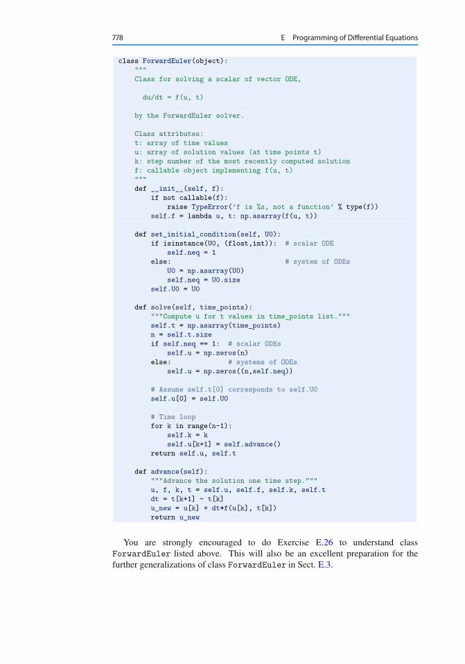
778 E Programming of Differential Equations
class ForwardEuler(object):
"""
Class for solving a scalar of vector ODE,
du/dt = f(u, t)
by the ForwardEuler solver.
Class attributes:
t: array of time values
u: array of solution values (at time points t)
k: step number of the most recently computed solution
f: callable object implementing f(u, t)
"""
def __init__(self, f):
if not callable(f):
raise TypeError(’f is %s, not a function’ % type(f))
self.f = lambda u, t: np.asarray(f(u, t))
def set_initial_condition(self, U0):
if isinstance(U0, (float,int)): # scalar ODE
self.neq = 1
else: # system of ODEs
U0 = np.asarray(U0)
self.neq = U0.size
self.U0 = U0
def solve(self, time_points):
"""Compute u for t values in time_points list."""
self.t = np.asarray(time_points)
n = self.t.size
if self.neq == 1: # scalar ODEs
self.u = np.zeros(n)
else: # systems of ODEs
self.u = np.zeros((n,self.neq))
# Assume self.t[0] corresponds to self.U0
self.u[0] = self.U0
# Time loop
for k in range(n-1):
self.k = k
self.u[k+1] = self.advance()
return self.u, self.t
def advance(self):
"""Advance the solution one time step."""
u, f, k, t = self.u, self.f, self.k, self.t
dt = t[k+1] - t[k]
u_new = u[k] + dt*f(u[k], t[k])
return u_new
You are strongly encouraged to do Exercise E.26 to understand classForwardEuler listed above. This will also be an excellent preparation for thefurther generalizations of class ForwardEuler in Sect. E.3.
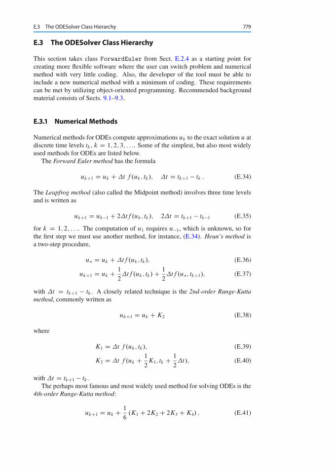
E.3 The ODESolver Class Hierarchy 779
E.3 The ODESolver Class Hierarchy
This section takes class ForwardEuler from Sect. E.2.4 as a starting point forcreating more flexible software where the user can switch problem and numericalmethod with very little coding. Also, the developer of the tool must be able toinclude a new numerical method with a minimum of coding. These requirementscan be met by utilizing object-oriented programming. Recommended backgroundmaterial consists of Sects. 9.1–9.3.
E.3.1 Numerical Methods
Numerical methods for ODEs compute approximations uk to the exact solution u atdiscrete time levels tk , k D 1; 2; 3; : : :. Some of the simplest, but also most widelyused methods for ODEs are listed below.
The Forward Euler method has the formula
ukC1 D uk C �t f .uk; tk/; �t D tkC1 � tk : (E.34)
The Leapfrog method (also called the Midpoint method) involves three time levelsand is written as
ukC1 D uk�1 C 2�tf .uk; tk/; 2�t D tkC1 � tk�1 (E.35)
for k D 1; 2; : : :. The computation of u1 requires u�1, which is unknown, so forthe first step we must use another method, for instance, (E.34). Heun’s method isa two-step procedure,
u� D uk C �tf .uk; tk/; (E.36)
ukC1 D uk C 1
2�tf .uk; tk/ C 1
2�tf .u�; tkC1/; (E.37)
with �t D tkC1 � tk . A closely related technique is the 2nd-order Runge-Kuttamethod, commonly written as
ukC1 D uk C K2 (E.38)
where
K1 D �t f .uk; tk/; (E.39)
K2 D �t f .uk C 1
2K1; tk C 1
2�t/; (E.40)
with �t D tkC1 � tk .The perhaps most famous and most widely used method for solving ODEs is the
4th-order Runge-Kutta method:
ukC1 D uk C 1
6.K1 C 2K2 C 2K3 C K4/ ; (E.41)
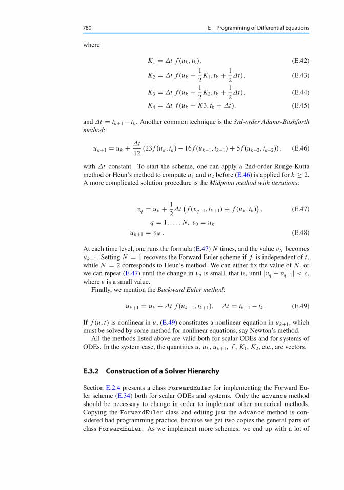
780 E Programming of Differential Equations
where
K1 D �t f .uk; tk/; (E.42)
K2 D �t f .uk C 1
2K1; tk C 1
2�t/; (E.43)
K3 D �t f .uk C 1
2K2; tk C 1
2�t/; (E.44)
K4 D �t f .uk C K3; tk C �t/; (E.45)
and �t D tkC1 � tk . Another common technique is the 3rd-order Adams-Bashforthmethod:
ukC1 D uk C �t
12.23f .uk; tk/ � 16f .uk�1; tk�1/ C 5f .uk�2; tk�2// ; (E.46)
with �t constant. To start the scheme, one can apply a 2nd-order Runge-Kuttamethod or Heun’s method to compute u1 and u2 before (E.46) is applied for k � 2.A more complicated solution procedure is the Midpoint method with iterations:
vq D uk C 1
2�t�f .vq�1; tkC1/ C f .uk; tk/
�; (E.47)
q D 1; : : : ; N; v0 D uk
ukC1 D vN : (E.48)
At each time level, one runs the formula (E.47) N times, and the value vN becomesukC1. Setting N D 1 recovers the Forward Euler scheme if f is independent of t ,while N D 2 corresponds to Heun’s method. We can either fix the value of N , orwe can repeat (E.47) until the change in vq is small, that is, until jvq � vq�1j < �,where � is a small value.
Finally, we mention the Backward Euler method:
ukC1 D uk C �t f .ukC1; tkC1/; �t D tkC1 � tk : (E.49)
If f .u; t/ is nonlinear in u, (E.49) constitutes a nonlinear equation in ukC1, whichmust be solved by some method for nonlinear equations, say Newton’s method.
All the methods listed above are valid both for scalar ODEs and for systems ofODEs. In the system case, the quantities u, uk, ukC1, f , K1, K2, etc., are vectors.
E.3.2 Construction of a Solver Hierarchy
Section E.2.4 presents a class ForwardEuler for implementing the Forward Eu-ler scheme (E.34) both for scalar ODEs and systems. Only the advance methodshould be necessary to change in order to implement other numerical methods.Copying the ForwardEuler class and editing just the advance method is con-sidered bad programming practice, because we get two copies the general parts ofclass ForwardEuler. As we implement more schemes, we end up with a lot of
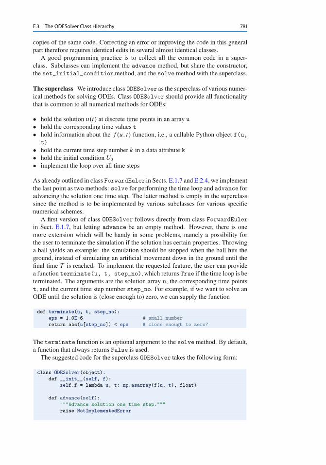
E.3 The ODESolver Class Hierarchy 781
copies of the same code. Correcting an error or improving the code in this generalpart therefore requires identical edits in several almost identical classes.
A good programming practice is to collect all the common code in a super-class. Subclasses can implement the advance method, but share the constructor,the set_initial_conditionmethod, and the solvemethod with the superclass.
The superclass We introduce class ODESolver as the superclass of various numer-ical methods for solving ODEs. Class ODESolver should provide all functionalitythat is common to all numerical methods for ODEs:
hold the solution u.t/ at discrete time points in an array u hold the corresponding time values t hold information about the f .u; t/ function, i.e., a callable Python object f(u,
t) hold the current time step number k in a data attribute k hold the initial condition U0
implement the loop over all time steps
As already outlined in class ForwardEuler in Sects. E.1.7 and E.2.4, we implementthe last point as two methods: solve for performing the time loop and advance foradvancing the solution one time step. The latter method is empty in the superclasssince the method is to be implemented by various subclasses for various specificnumerical schemes.
A first version of class ODESolver follows directly from class ForwardEulerin Sect. E.1.7, but letting advance be an empty method. However, there is onemore extension which will be handy in some problems, namely a possibility forthe user to terminate the simulation if the solution has certain properties. Throwinga ball yields an example: the simulation should be stopped when the ball hits theground, instead of simulating an artificial movement down in the ground until thefinal time T is reached. To implement the requested feature, the user can providea function terminate(u, t, step_no), which returns True if the time loop is beterminated. The arguments are the solution array u, the corresponding time pointst, and the current time step number step_no. For example, if we want to solve anODE until the solution is (close enough to) zero, we can supply the function
def terminate(u, t, step_no):
eps = 1.0E-6 # small number
return abs(u[step_no]) < eps # close enough to zero?
The terminate function is an optional argument to the solvemethod. By default,a function that always returns False is used.
The suggested code for the superclass ODESolver takes the following form:
class ODESolver(object):
def __init__(self, f):
self.f = lambda u, t: np.asarray(f(u, t), float)
def advance(self):
"""Advance solution one time step."""
raise NotImplementedError
782 E Programming of Differential Equations
def set_initial_condition(self, U0):
if isinstance(U0, (float,int)): # scalar ODE
self.neq = 1
U0 = float(U0)
else: # system of ODEs
U0 = np.asarray(U0)
self.neq = U0.size
self.U0 = U0
def solve(self, time_points, terminate=None):
if terminate is None:
terminate = lambda u, t, step_no: False
self.t = np.asarray(time_points)
n = self.t.size
if self.neq == 1: # scalar ODEs
self.u = np.zeros(n)
else: # systems of ODEs
self.u = np.zeros((n,self.neq))
# Assume that self.t[0] corresponds to self.U0
self.u[0] = self.U0
# Time loop
for k in range(n-1):
self.k = k
self.u[k+1] = self.advance()
if terminate(self.u, self.t, self.k+1):
break # terminate loop over k
return self.u[:k+2], self.t[:k+2]
Note that we return just the parts of self.u and self.t that have been filled withvalues (the rest are zeroes): all elements up to the one with index k+1 are computedbefore terminate may return True. The corresponding slice of the array is then:k+2 since the upper limit is not included in the slice. If terminate never returnsTrue we simply have that :k+1 is the entire array.
The Forward Euler method Subclasses implement specific numerical formulasfor numerical solution of ODEs in the advancemethod. The Forward Euler scheme(E.34) is implemented by defining the subclass name and copying the advancemethod from the ForwardEuler class in Sect. E.1.7 or E.1.7:
class ForwardEuler(ODESolver):
def advance(self):
u, f, k, t = self.u, self.f, self.k, self.t
dt = t[k+1] - t[k]
u_new = u[k] + dt*f(u[k], t[k])
return u_new
Remark on stripping off the self prefixWhen we extract data attributes to local variables with short names, we shouldonly use these local variables for reading values, not setting values. For example,if we do a k += 1 to update the time step counter, that increased value is not re-flected in self.k (which is the “official” counter). On the other hand, changing
E.3 The ODESolver Class Hierarchy 783
a list in-place, say u[k+1] = ..., is reflected in self.u. Extracting data at-tributes in local variables is done for getting the code closer to the mathematics,but has a danger of introducing bugs that might be hard to track down.
The 4th-order Runge-Kutta method Below is an implementation of the 4th-orderRunge-Kutta method (E.41):
class RungeKutta4(ODESolver):
def advance(self):
u, f, k, t = self.u, self.f, self.k, self.t
dt = t[k+1] - t[k]
dt2 = dt/2.0
K1 = dt*f(u[k], t[k])
K2 = dt*f(u[k] + 0.5*K1, t[k] + dt2)
K3 = dt*f(u[k] + 0.5*K2, t[k] + dt2)
K4 = dt*f(u[k] + K3, t[k] + dt)
u_new = u[k] + (1/6.0)*(K1 + 2*K2 + 2*K3 + K4)
return u_new
It is left as exercises to implement other numerical methods in the ODESolverclass hierarchy. However, the Backward Euler method (E.49) requires a much moreadvanced implementation than the other methods so that particular method deservesits own section.
E.3.3 The Backward Euler Method
The Backward Euler scheme (E.49) leads in general to a nonlinear equation at a newtime level, while all the other schemes listed in Sect. E.3.1 have a simple formulafor the new ukC1 value. The nonlinear equation reads
ukC1 D uk C �t f .ukC1; tkC1/ :
For simplicity we assume that the ODE is scalar so the unknown ukC1 is a scalar.It might be easier to see that the equation for ukC1 is nonlinear if we rearrange theequation to
F.w/ w � �tf .w; tkC1/ � uk D 0; (E.50)
where w D ukC1. If now f .u; t/ is a nonlinear function of u, F.w/ will also bea nonlinear function of w.
To solve F.w/ D 0 we can use the Bisection method from Sect. 4.11.2, New-ton’s method from Sect. A.1.10, or the Secant method from Exercise A.10. Here weapply Newton’s method and the implementation given in src/diffeq/Newton.py.A disadvantage with Newton’s method is that we need the derivative of F with re-spect to w, which requires the derivative @f .w; t/=@w. A quick solution is to usea numerical derivative, e.g., class Derivative from Sect. 7.3.2.
We make a subclass BackwardEuler. As we need to solve F.w/ D 0 at everytime step, we also need to implement the F.w/ function. This is conveniently donein a local function inside the advancemethod:
784 E Programming of Differential Equations
def advance(self):
u, f, k, t = self.u, self.f, self.k, self.t
def F(w):
return w - dt*f(w, t[k+1]) - u[k]
dFdw = Derivative(F)
w_start = u[k] + dt*f(u[k], t[k]) # Forward Euler step
u_new, n, F_value = self.Newton(F, w_start, dFdw, N=30)
if n >= 30:
print "Newton’s failed to converge at t=%g "\
"(%d iterations)" % (t, n)
return u_new
The local variables in the advance function, such as dt and u, act as “global”variables for the F function. Hence, when F is sent away to some self.Newtonfunction, F remembers the values of dt, f, t, and u (!). The derivative dF=dw isin our advance function computed numerically by a class Derivative, which isa slight modification of the similar class in Sect. 7.3.2, because we now want to usea more accurate, centered formula:
class Derivative(object):
def __init__(self, f, h=1E-5):
self.f = f
self.h = float(h)
def __call__(self, x):
f, h = self.f, self.h
return (f(x+h) - f(x-h))/(2*h)
This code is included in the ODESolver.py file.The next step is to call Newton’s method. For this purpose we need to import
the Newton function from the Newton module. The Newton.py file must thenreside in the same directory as ODESolver.py, or Newton.py must be in one ofthe directories listed in the sys.path list or the PYTHONPATH environment variable(see Sect. 4.9.7).
Having the Newton(f, x_start, dfdx, N) function from Sect. A.1.10 ac-cessible in our ODESolver.py file, we can make a call and supply our F function asthe argument f, a start value for the iteration, here called w_start, as the argumentx, and the derivative dFdw for the argument dfdx. We rely on default values for theepsilon and store arguments, while the maximum number of iterations is set toN=30. The program is terminated if it happens that the number of iterations exceedsthat value, because then the method is not considered to have converged (at leastnot quickly enough), and we have consequently not been able to compute the nextukC1 value.
The starting value for Newton’s method must be chosen. As we expect the so-lution to not change much from one time level to the next, uk could be a goodinitial guess. However, we can do better by using a simple Forward Euler stepuk C �tf .uk; tk/, which is exactly what we do in the advance function above.
E.3 The ODESolver Class Hierarchy 785
Since Newton’s method always has the danger of converging slowly, it can beinteresting to store the number of iterations at each time level as a data attribute inthe BackwardEuler class. We can easily insert extra statement for this purpose:
def advance(self):
...
u_new, n, F_value = Newton(F, w_start, dFdw, N=30)
if k == 0:
self.Newton_iter = []
self.Newton_iter.append(n)
...
Note the need for creating an empty list (at the first call of advance) before we canappend elements.
There is now one important question to ask: will the advancemethod work forsystems of ODEs? In that case, F.w/ is a vector of functions. The implementa-tion of F will work when w is a vector, because all the quantities involved in theformula are arrays or scalar variables. The dFdw instance will compute a numeri-cal derivative of each component of the vector function dFdw.f (which is simplyour F function). The call to the Newton function is more critical: It turns out thatthis function, as the algorithm behind it, works for scalar equations only. Newton’smethod can quite easily be extended to a system of nonlinear equations, but we donot consider that topic here. Instead we equip class BackwardEuler with a con-structor that calls the f object and controls that the returned value is a float andnot an array:
class BackwardEuler(ODESolver):
def __init__(self, f):
ODESolver.__init__(self, f)
# Make a sample call to check that f is a scalar function:
try:
u = np.array([1]); t = 1
value = f(u, t)
except IndexError: # index out of bounds for u
raise ValueError(’f(u,t) must return float/int’)
Observe that we must explicitly call the superclass constructor and pass on theargument f to achieve the right storage and treatment of this argument.
Understanding class BackwardEuler implies a good understanding of classesin general; a good understanding of numerical methods for ODEs, for numericaldifferentiation, and for finding roots of functions; and a good understanding on howto combine different code segments from different parts of the book. Therefore, ifyou have digested class BackwardEuler, you have all reasons to believe that youhave digested the key topics of this book.
E.3.4 Verification
The fundamental problemwith testing approximate numerical methods is that we donot normally know what the output from the computer should be. In some special
786 E Programming of Differential Equations
cases, however, we can find an exact solution of the discretized problem that thecomputer program solves. This exact solution should be reproduced to machineprecision by the program. It turns out that most numerical methods for ordinarydifferential equations are able to exactly reproduce a linear solution. That is, ifthe solution of the differential equation is u D at C b, the numerical method willproduce the same solution: uk D ak�t C b. We can use this knowledge to makea test function for verifying our implementations.
Let u D at C b be the solution of the test problem. A corresponding ODE isobviously u0 D a, with u.0/ D b. A more demanding ODE arises from addinga term that is zero, e.g., .u � .at C b//5. We therefore aim to solve
u0 D a C .u � .at C b//5; u.0/ D b :
Our test function loops over registered solvers in the ODESolver hierarchy,solves the test problem, and checks that the maximum deviation between the com-puted solution and the exact linear solution is within a tolerance:
registered_solver_classes = [
ForwardEuler, RungeKutta4, BackwardEuler]
def test_exact_numerical_solution():
a = 0.2; b = 3
def f(u, t):
return a + (u - u_exact(t))**5
def u_exact(t):
"""Exact u(t) corresponding to f above."""
return a*t + b
U0 = u_exact(0)
T = 8
n = 10
tol = 1E-15
t_points = np.linspace(0, T, n)
for solver_class in registered_solver_classes:
solver = solver_class(f)
solver.set_initial_condition(U0)
u, t = solver.solve(t_points)
u_e = u_exact(t)
max_error = (u_e - u).max()
msg = ’%s failed with max_error=%g’ % \
(solver.__class__.__name__, max_error)
assert max_error < tol, msg
Note how we can make a loop over class types (because the class is an ordinaryobject in Python). New subclasses can add their class type to the registered_solver_classes list and the test function will include such new classes in the testas well.
Remarks A more general testing technique is based on knowing how the error ina numerical method varies with the discretization parameter, here �t . Say we know
E.3 The ODESolver Class Hierarchy 787
that a particular method has an error that decays as �t2. In a problem where theexact analytical solution is known, we can run the numerical method for severalvalues of �t and compute the corresponding numerical error in each case. If thecomputed errors decay like �t2, it brings quite strong evidence for a correct imple-mentation. Such tests are called convergence tests and constitute the most generaltool we have for verifying implementations of numerical algorithms. Exercise E.37gives an introduction to the topic.
E.3.5 Example: Exponential Decay
Let us apply the classes in the ODESolver hierarchy to see how they solve theperhaps simplest of all ODEs: u0 D �u, with initial condition u.0/ D 1. The exactsolution is u.t/ D e�t , which decays exponentially with time. Application of classForwardEuler to solve this problem requires writing the following code:
import ODESolver
def f(u, t):
return -u
solver = ODESolver.ForwardEuler(f)
solver.set_initial_condition(1.0)
t_points = linspace(0, 3, 31)
u, t = solver.solve(t_points)
plot(t, u)
We can run various values of �t to see the effect on the accuracy:
# Test various dt values and plot
figure()
legends = []
T = 3
for dt in 2.0, 1.0, 0.5, 0.1:
n = int(round(T/dt))
solver = ODESolver.ForwardEuler(f)
solver.set_initial_condition(1)
u, t = solver.solve(linspace(0, T, n+1))
plot(t, u)
legends.append(’dt=%g’ % dt)
hold(’on’)
plot(t, exp(-t), ’bo’)
legends.append(’exact’)
legend(legends)
Figure E.4 shows alarming results. With �t D 2 we get a completely wrong solu-tion that becomes negative and then increasing. The value �t D 1 gives a peculiarsolution: uk D 0 for k � 1! Qualitatively correct behavior appears with �t D 0:5,and the results get quantitatively better as we decrease �t . The solution correspond-ing to � D 0:1 looks good from the graph.
Such strange results reveal that we most likely have programming errors in ourimplementation. Fortunately, we did some verification of the implementations in
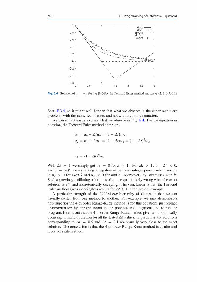
788 E Programming of Differential Equations
-0.6
-0.4
-0.2
0
0.2
0.4
0.6
0.8
1
0 0.5 1 1.5 2 2.5 3
dt=2dt=1
dt=0.5dt=0.1exact
Fig. E.4 Solution of u0 D �u for t 2 Œ0; 3� by the Forward Euler method and �t 2 f2; 1; 0:5; 0:1g
Sect. E.3.4, so it might well happen that what we observe in the experiments areproblems with the numerical method and not with the implementation.
We can in fact easily explain what we observe in Fig. E.4. For the equation inquestion, the Forward Euler method computes
u1 D u0 � �tu0 D .1 � �t/u0;
u2 D u1 � �tu1 D .1 � �t/u1 D .1 � �t/2u0;
:::
uk D .1 � �t/ku0 :
With �t D 1 we simply get uk D 0 for k � 1. For �t > 1, 1 � �t < 0,and .1 � �t/k means raising a negative value to an integer power, which resultsin uk > 0 for even k and uk < 0 for odd k. Moreover, jukj decreases with k.Such a growing, oscillating solution is of course qualitatively wrong when the exactsolution is e�t and monotonically decaying. The conclusion is that the ForwardEuler method gives meaningless results for �t � 1 in the present example.
A particular strength of the ODESolver hierarchy of classes is that we cantrivially switch from one method to another. For example, we may demonstratehow superior the 4-th order Runge-Kutta method is for this equation: just replaceForwardEuler by RungeKutta4 in the previous code segment and re-run theprogram. It turns out that the 4-th order Runge-Kutta method gives a monotonicallydecaying numerical solution for all the tested �t values. In particular, the solutionscorresponding to �t D 0:5 and �t D 0:1 are visually very close to the exactsolution. The conclusion is that the 4-th order Runge-Kutta method is a safer andmore accurate method.
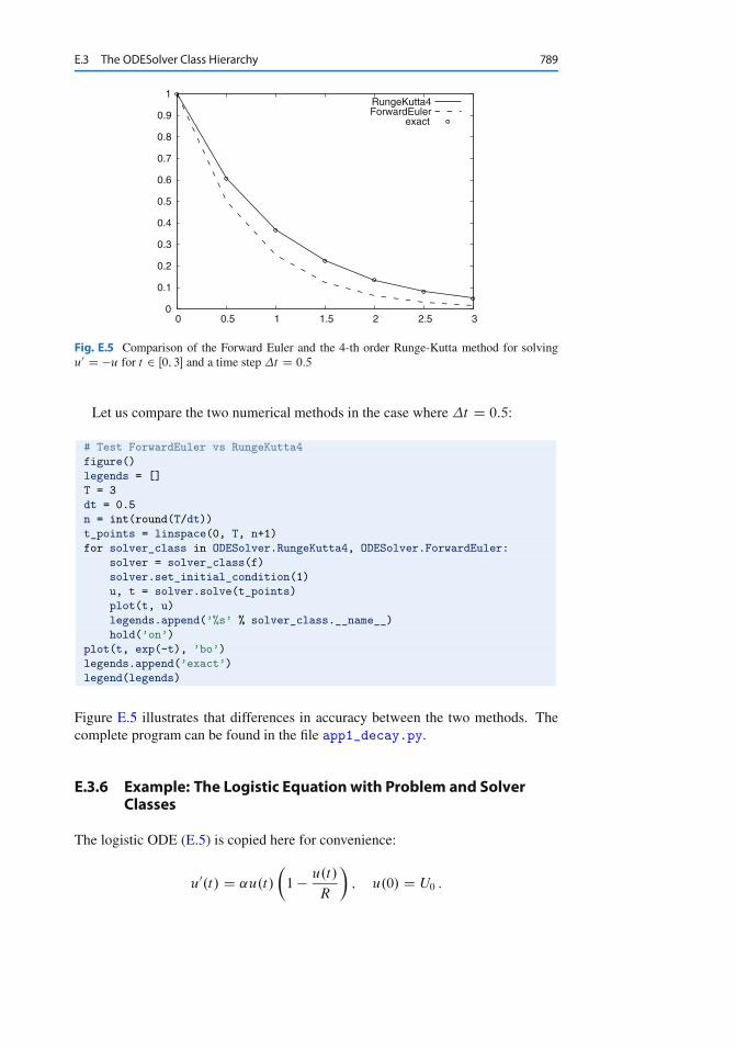
E.3 The ODESolver Class Hierarchy 789
0
0.1
0.2
0.3
0.4
0.5
0.6
0.7
0.8
0.9
1
0 0.5 1 1.5 2 2.5 3
RungeKutta4ForwardEuler
exact
Fig. E.5 Comparison of the Forward Euler and the 4-th order Runge-Kutta method for solvingu0 D �u for t 2 Œ0; 3� and a time step �t D 0:5
Let us compare the two numerical methods in the case where �t D 0:5:
# Test ForwardEuler vs RungeKutta4
figure()
legends = []
T = 3
dt = 0.5
n = int(round(T/dt))
t_points = linspace(0, T, n+1)
for solver_class in ODESolver.RungeKutta4, ODESolver.ForwardEuler:
solver = solver_class(f)
solver.set_initial_condition(1)
u, t = solver.solve(t_points)
plot(t, u)
legends.append(’%s’ % solver_class.__name__)
hold(’on’)
plot(t, exp(-t), ’bo’)
legends.append(’exact’)
legend(legends)
Figure E.5 illustrates that differences in accuracy between the two methods. Thecomplete program can be found in the file app1_decay.py.
E.3.6 Example: The Logistic Equation with Problem and SolverClasses
The logistic ODE (E.5) is copied here for convenience:
u0.t/ D ˛u.t/
�1 � u.t/
R
�; u.0/ D U0 :
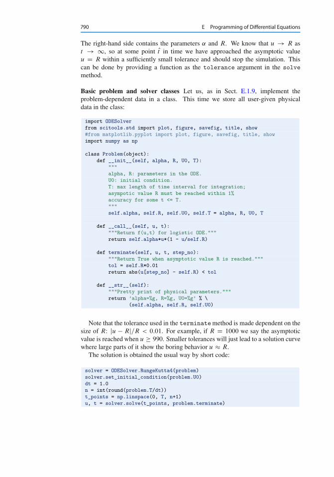
790 E Programming of Differential Equations
The right-hand side contains the parameters ˛ and R. We know that u ! R ast ! 1, so at some point Ot in time we have approached the asymptotic valueu D R within a sufficiently small tolerance and should stop the simulation. Thiscan be done by providing a function as the tolerance argument in the solvemethod.
Basic problem and solver classes Let us, as in Sect. E.1.9, implement theproblem-dependent data in a class. This time we store all user-given physicaldata in the class:
import ODESolver
from scitools.std import plot, figure, savefig, title, show
#from matplotlib.pyplot import plot, figure, savefig, title, show
import numpy as np
class Problem(object):
def __init__(self, alpha, R, U0, T):
"""
alpha, R: parameters in the ODE.
U0: initial condition.
T: max length of time interval for integration;
asympotic value R must be reached within 1%
accuracy for some t <= T.
"""
self.alpha, self.R, self.U0, self.T = alpha, R, U0, T
def __call__(self, u, t):
"""Return f(u,t) for logistic ODE."""
return self.alpha*u*(1 - u/self.R)
def terminate(self, u, t, step_no):
"""Return True when asymptotic value R is reached."""
tol = self.R*0.01
return abs(u[step_no] - self.R) < tol
def __str__(self):
"""Pretty print of physical parameters."""
return ’alpha=%g, R=%g, U0=%g’ % \
(self.alpha, self.R, self.U0)
Note that the tolerance used in the terminatemethod is made dependent on thesize of R: ju � Rj=R < 0:01. For example, if R D 1000 we say the asymptoticvalue is reached when u � 990. Smaller tolerances will just lead to a solution curvewhere large parts of it show the boring behavior u � R.
The solution is obtained the usual way by short code:
solver = ODESolver.RungeKutta4(problem)
solver.set_initial_condition(problem.U0)
dt = 1.0
n = int(round(problem.T/dt))
t_points = np.linspace(0, T, n+1)
u, t = solver.solve(t_points, problem.terminate)
E.3 The ODESolver Class Hierarchy 791
Let us pack these statements into a class Solver, which has two methods: solveand plot, and add some documentation and flexibility. The code may look like
class Solver(object):
def __init__(self, problem, dt,
method=ODESolver.ForwardEuler):
"""
problem: instance of class Problem.
dt: time step.
method: class in ODESolver hierarchy.
"""
self.problem, self.dt = problem, dt
self.solver = method
def solve(self):
solver = self.method(self.problem)
solver.set_initial_condition(self.problem.U0)
n = int(round(self.problem.T/self.dt))
t_points = np.linspace(0, self.problem.T, n+1)
self.u, self.t = solver.solve(t_points,
self.problem.terminate)
# The solution terminated if the limiting value was reached
if solver.k+1 == n: # no termination - we reached final T
self.plot()
raise ValueError(
’termination criterion not reached, ’\
’give T > %g’ % self.problem.T)
def plot(self):
filename = ’logistic_’ + str(self.problem) + ’.pdf’
plot(self.t, self.u)
title(str(self.problem) + ’, dt=%g’ % self.dt)
savefig(filename)
show()
Problem-dependent data related to the numerical quality of the solution, such asthe time step here, go to the Solver class. That is, class Problem contains thephysics and class Solver the numerics of the problem under investigation.
If the last computed time step, solver.k+1, equals the last possible index, n,problem.terminate never returned True, which means that the asymptotic limitwas not reached. This is treated as an erroneous condition. To guide the user,we launch a plot before raising the exception with an instructive message. Thecomplete code is found in the file app2_logistic.py.
Computing an appropriate �t Choosing an appropriate�t is not always so easy.The impact of �t can sometimes be dramatic, as demonstrated for the ForwardEuler method in Sect. E.3.5. We could automate the process of finding a suitable�t : start with a large �t , and keep halving �t until the difference between twosolutions corresponding to two consequtive �t values is small enough.
Say solver is a class Solver instance computed with time step �t andsolver2 is the instance corresponding to a computation with �t=2. Calculat-ing the difference between solver.u and solver2.u is not trivial as one of the
792 E Programming of Differential Equations
arrays has approximately twice as many elements as the other, and the last elementin both arrays does not necessarily correspond to the same time value since the timestepping and the terminate function may lead to slightly different terminationtimes.
A solution to these two problems is to turn each of the arrays solver.uand solver2.u into continuous functions, as explained in Sect. E.1.5, and thenevaluate the difference at some selected time points up to the smallest value ofsolver.t[-1] and solver2.t[-1]. The code becomes
# Make continuous functions u(t) and u2(t)
u = wrap2callable((solver. t, solver. u))
u2 = wrap2callable((solver2.t, solver2.u))
# Sample the difference in n points in [0, t_end]
n = 13
t_end = min(solver2.t[-1], solver.t[-1])
t = np.linspace(0, t_end, n)
u_diff = np.abs(u(t) - u2(t)).max()
The next step is to introduce a loop where we halve the time step in each iterationand solve the logistic ODE with the new time step and compute u_diff as shownabove. A complete function takes the form
def find_dt(problem, method=ODESolver.ForwardEuler,
tol=0.01, dt_min=1E-6):
"""
Return a "solved" class Solver instance where the
difference in the solution and one with a double
time step is less than tol.
problem: class Problem instance.
method: class in ODESolver hierarchy.
tol: tolerance (chosen relative to problem.R).
dt_min: minimum allowed time step.
"""
dt = problem.T/10 # start with 10 intervals
solver = Solver(problem, dt, method)
solver.solve()
from scitools.std import wrap2callable
good_approximation = False
while not good_approximation:
dt = dt/2.0
if dt < dt_min:
raise ValueError(’dt=%g < %g - abort’ % (dt, dt_min))
solver2 = Solver(problem, dt, method)
solver2.solve()
# Make continuous functions u(t) and u2(t)
u = wrap2callable((solver. t, solver. u))
u2 = wrap2callable((solver2.t, solver2.u))
# Sample the difference in n points in [0, t_end]
n = 13
t_end = min(solver2.t[-1], solver.t[-1])
E.3 The ODESolver Class Hierarchy 793
t = np.linspace(0, t_end, n)
u_diff = np.abs(u(t) - u2(t)).max()
print u_diff, dt, tol
if u_diff < tol:
good_approximation = True
else:
solver = solver2
return solver2
Setting the tolerance tol must be done with a view to the typical size of u,i.e., the size of R. With R D 100 and tol=1, the Forward Euler method meetsthe tolerance for �t D 0:25. Switching to the 4-th order Runge-Kutta methodmakes �t D 1:625 sufficient to meet the tolerance. Note that although the lattermethod can use a significantly larger time step, it also involves four times as manyevaluations of the right-hand side function at each time step.
Finally, we show how to make a class that behaves as class Solver, but withautomatic computation of the time step. If we do not provide a dt parameter tothe constructor, the find_dt function just presented is used to compute dt and thesolution, otherwise we use the standard Solver.solve code. This new class isconveniently realized as a subclass of Solver where we override the constructorand the solvemethod. The plotmethod can be inherited as is. The code becomes
class AutoSolver(Solver):
def __init__(self, problem, dt=None,
method=ODESolver.ForwardEuler,
tol=0.01, dt_min=1E-6):
Solver.__init__(self, problem, dt, method)
if dt is None:
solver = find_dt(self.problem, method,
tol, dt_min)
self.dt = solver.dt
self.u, self.t = solver.u, solver.t
def solve(self, method=ODESolver.ForwardEuler):
if hasattr(self, ’u’):
# Solution was computed by find_dt in constructor
pass
else:
Solver.solve(self)
The call hasattr(self, ’u’) returns True if u is a data attribute in objectself. Here this is used as an indicator that the solution was computed in the con-structor by the find_dt function. A typical use is
problem = Problem(alpha=0.1, R=500, U0=2, T=130)
solver = AutoSolver(problem, tol=1)
solver.solve(method=ODESolver.RungeKutta4)
solver.plot()
Dealing with time-dependent coefficients The carrying capacity of the environ-ment, R, may vary with time, e.g., due to seasonal changes. Can we extend the
794 E Programming of Differential Equations
previous code so that R can be specified either as a constant or as a function oftime?
This is in fact easy if we in the implementation of the right-hand side functionassume that R is a function of time. If R is given as a constant in the constructor ofclass Problem, we just wrap it as a function of time:
if isinstance(R, (float,int)): # number?
self.R = lambda t: R
elif callable(R):
self.R = R
else:
raise TypeError(
’R is %s, has to be number of function’ % type(R))
The terminatemethod is also affected as we need to base the tolerance on the R
value at the present time level. Also the __str__method must be changed since itis not meaningful to print a function self.R. That is, all methods in the generalizedproblem class, here called Problem2, must be altered. We have not chosen to makeProblem2 a subclass of Problem, even though the interface is the same and the twoclasses are closely related. While Problem is clearly a special case of Problem2,as a constant R is a special case of a function .R/, the opposite case is not true.
Class Problem2 becomes
class Problem2(Problem):
def __init__(self, alpha, R, U0, T):
"""
alpha, R: parameters in the ODE.
U0: initial condition.
T: max length of time interval for integration;
asympotic value R must be reached within 1%
accuracy for some t <= T.
"""
self.alpha, self.U0, self.T = alpha, U0, T
if isinstance(R, (float,int)): # number?
self.R = lambda t: R
elif callable(R):
self.R = R
else:
raise TypeError(
’R is %s, has to be number of function’ % type(R))
def __call__(self, u, t):
"""Return f(u,t) for logistic ODE."""
return self.alpha*u*(1 - u/self.R(t))
def terminate(self, u, t, step_no):
"""Return True when asymptotic value R is reached."""
tol = self.R(t[step_no])*0.01
return abs(u[step_no] - self.R(t[step_no])) < tol
def __str__(self):
return ’alpha=%g, U0=%g’ % (self.alpha, self.U0)
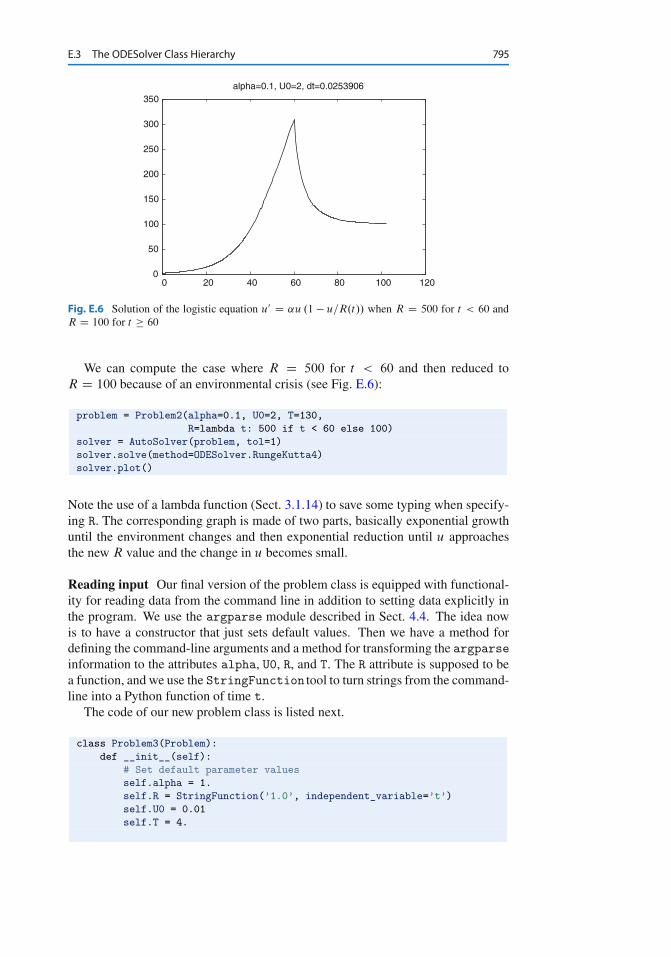
E.3 The ODESolver Class Hierarchy 795
0
50
100
150
200
250
300
350
0 20 40 60 80 100 120
alpha=0.1, U0=2, dt=0.0253906
Fig. E.6 Solution of the logistic equation u0 D ˛u .1 � u=R.t// when R D 500 for t < 60 andR D 100 for t � 60
We can compute the case where R D 500 for t < 60 and then reduced toR D 100 because of an environmental crisis (see Fig. E.6):
problem = Problem2(alpha=0.1, U0=2, T=130,
R=lambda t: 500 if t < 60 else 100)
solver = AutoSolver(problem, tol=1)
solver.solve(method=ODESolver.RungeKutta4)
solver.plot()
Note the use of a lambda function (Sect. 3.1.14) to save some typing when specify-ing R. The corresponding graph is made of two parts, basically exponential growthuntil the environment changes and then exponential reduction until u approachesthe new R value and the change in u becomes small.
Reading input Our final version of the problem class is equipped with functional-ity for reading data from the command line in addition to setting data explicitly inthe program. We use the argparse module described in Sect. 4.4. The idea nowis to have a constructor that just sets default values. Then we have a method fordefining the command-line arguments and a method for transforming the argparseinformation to the attributes alpha, U0, R, and T. The R attribute is supposed to bea function, and we use the StringFunction tool to turn strings from the command-line into a Python function of time t.
The code of our new problem class is listed next.
class Problem3(Problem):
def __init__(self):
# Set default parameter values
self.alpha = 1.
self.R = StringFunction(’1.0’, independent_variable=’t’)
self.U0 = 0.01
self.T = 4.
796 E Programming of Differential Equations
def define_command_line_arguments(self, parser):
"""Add arguments to parser (argparse.ArgumentParser)."""
def evalcmlarg(text):
return eval(text)
def toStringFunction(text):
return StringFunction(text, independent_variable=’t’)
parser.add_argument(
’--alpha’, dest=’alpha’, type=evalcmlarg,
default=self.alpha,
help=’initial growth rate in logistic model’)
parser.add_argument(
’--R’, dest=’R’, type=toStringFunction, default=self.R,
help=’carrying capacity of the environment’)
parser.add_argument(
’--U0’, dest=’U0’, type=evalcmlarg, default=self.U0,
help=’initial condition’)
parser.add_argument(
’--T’, dest=’T’, type=evalcmlarg, default=self.T,
help=’integration in time interval [0,T]’)
return parser
def set(self, **kwargs):
"""
Set parameters as keyword arguments alpha, R, U0, or T,
or as args (object returned by parser.parse_args()).
"""
for prm in (’alpha’, ’U0’, ’R’, ’T’):
if prm in kwargs:
setattr(self, prm, kwargs[prm])
if ’args’ in kwargs:
args = kwargs[’args’]
for prm in (’alpha’, ’U0’, ’R’, ’T’):
if hasattr(args, prm):
setattr(self, prm, getattr(args, prm))
else:
print ’Really strange’, dir(args)
def __call__(self, u, t):
"""Return f(u,t) for logistic ODE."""
return self.alpha*u*(1 - u/self.R(t))
def terminate(self, u, t, step_no):
"""Return True when asymptotic value R is reached."""
tol = self.R(t[step_no])*0.01
return abs(u[step_no] - self.R(t[step_no])) < tol
def __str__(self):
s = ’alpha=%g, U0=%g’ % (self.alpha, self.U0)
if isinstance(self.R, StringFunction):
s += ’, R=%s’ % str(self.R)
return s
The calls to parser.add_argument are straightforward, but notice that weallow strings for ˛, U0, and T to be interpreted by eval. The string for R is in-
E.3 The ODESolver Class Hierarchy 797
terpreted as a formula by StringFunction. The setmethod is flexible: it acceptsany set of keyword arguments, and first checks if these are the names of the prob-lem parameters, and thereafter if args=’ is given, the parameters are taken fromthe command line. The rest of the class is very similar to earlier versions.
The typical use of class Problem3 is shown below. First we set parametersdirectly:
problem = Problem3()
problem.set(alpha=0.1, U0=2, T=130,
R=lambda t: 500 if t < 60 else 100)
solver = AutoSolver(problem, tol=1)
solver.solve(method=ODESolver.RungeKutta4)
solver.plot()
Then we rely on reading parameters from the command line:
problem = Problem3()
import argparse
parser = argparse.ArgumentParser(
description=’Logistic ODE model’)
parser = problem.define_command_line_arguments(parser)
# Try --alpha 0.11 --T 130 --U0 2 --R ’500 if t < 60 else 300’
args = parser.parse_args()
problem.set(args=args)
solver = AutoSolver(problem, tol=1)
solver.solve(method=ODESolver.RungeKutta4)
solver.plot()
The last example using a problem class integrated with the command line is themost flexible way of implementing ODE models.
E.3.7 Example: An Oscillating System
The motion of a box attached to a spring, as described in detail in Appendix D,can be modeled by two first-order differential equations as listed in (E.33), hererepeated with F.t/ D mw00.t/, where the w.t/ function is the forced movement ofthe end of the spring.
du.0/
dtD u.1/;
du.1/
dtD w00.t/ C g � m�1ˇu.1/ � m�1ku.0/ :
The code related to this example is found in app3_osc.py. Because our right-hand side f contains several parameters, we implement it as a class with the pa-rameters as data attributes and a __call__ method for returning the 2-vector f .We assume that the user of the class supplies the w.t/ function, so it is natural tocompute w00.t/ by a finite difference formula.
798 E Programming of Differential Equations
class OscSystem:
def __init__(self, m, beta, k, g, w):
self.m, self.beta, self.k, self.g, self.w = \
float(m), float(beta), float(k), float(g), w
def __call__(self, u, t):
u0, u1 = u
m, beta, k, g, w = \
self.m, self.beta, self.k, self.g, self.w
# Use a finite difference for w’’(t)
h = 1E-5
ddw = (w(t+h) - 2*w(t) + w(t-h))/(h**2)
f = [u1, ddw + g - beta/m*u1 - k/m*u0]
return f
A simple test case arises if we set m D k D 1 and ˇ D g D w D 0:
du.0/
dtD u.1/;
du.1/
dtD �u.0/ :
Suppose that u.0/.0/ D 1 and u.1/.0/ D 0. An exact solution is then
u.0/.t/ D cos t; u.1/.t/ D � sin t :
We can use this case to check how the Forward Euler method compares with the4-th order Runge-Kutta method:
import ODESolver
from scitools.std import *
#from matplotlib.pyplot import *
legends = []
f = OscSystem(1.0, 0.0, 1.0, 0.0, lambda t: 0)
u_init = [1, 0] # initial condition
nperiods = 3.5 # no of oscillation periods
T = 2*pi*nperiods
for solver_class in ODESolver.ForwardEuler, ODESolver.RungeKutta4:
if solver_class == ODESolver.ForwardEuler:
npoints_per_period = 200
elif solver_class == ODESolver.RungeKutta4:
npoints_per_period = 20
n = npoints_per_period*nperiods
t_points = linspace(0, T, n+1)
solver = solver_class(f)
solver.set_initial_condition(u_init)
u, t = solver.solve(t_points)
# u is an array of [u0,u1] pairs for each time level,
# get the u0 values from u for plotting
u0_values = u[:, 0]
u1_values = u[:, 1]
u0_exact = cos(t)
u1_exact = -sin(t)
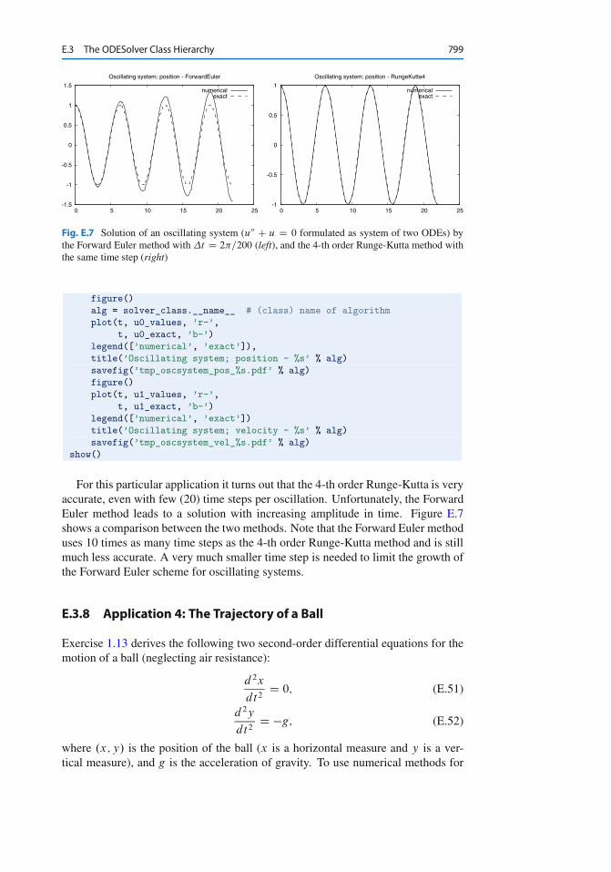
E.3 The ODESolver Class Hierarchy 799
-1.5
-1
-0.5
0
0.5
1
1.5
0 5 10 15 20 25
Oscillating system; position - ForwardEuler
numericalexact
-1
-0.5
0
0.5
1
0 5 10 15 20 25
Oscillating system; position - RungeKutta4
numericalexact
Fig. E.7 Solution of an oscillating system (u00 C u D 0 formulated as system of two ODEs) bythe Forward Euler method with �t D 2�=200 (left), and the 4-th order Runge-Kutta method withthe same time step (right)
figure()
alg = solver_class.__name__ # (class) name of algorithm
plot(t, u0_values, ’r-’,
t, u0_exact, ’b-’)
legend([’numerical’, ’exact’]),
title(’Oscillating system; position - %s’ % alg)
savefig(’tmp_oscsystem_pos_%s.pdf’ % alg)
figure()
plot(t, u1_values, ’r-’,
t, u1_exact, ’b-’)
legend([’numerical’, ’exact’])
title(’Oscillating system; velocity - %s’ % alg)
savefig(’tmp_oscsystem_vel_%s.pdf’ % alg)
show()
For this particular application it turns out that the 4-th order Runge-Kutta is veryaccurate, even with few (20) time steps per oscillation. Unfortunately, the ForwardEuler method leads to a solution with increasing amplitude in time. Figure E.7shows a comparison between the two methods. Note that the Forward Euler methoduses 10 times as many time steps as the 4-th order Runge-Kutta method and is stillmuch less accurate. A very much smaller time step is needed to limit the growth ofthe Forward Euler scheme for oscillating systems.
E.3.8 Application 4: The Trajectory of a Ball
Exercise 1.13 derives the following two second-order differential equations for themotion of a ball (neglecting air resistance):
d 2x
dt2D 0; (E.51)
d 2y
dt2D �g; (E.52)
where .x; y/ is the position of the ball (x is a horizontal measure and y is a ver-tical measure), and g is the acceleration of gravity. To use numerical methods for
800 E Programming of Differential Equations
first-order equations, we must rewrite the system of two second-order equationsas a system of four first-order equations. This is done by introducing to new un-knowns, the velocities vx D dx=dt and vy D dy=dt . We then have the first-ordersystem of ODEs
dx
dtD vx; (E.53)
dvx
dtD 0; (E.54)
dy
dtD vy; (E.55)
dvy
dtD �g : (E.56)
The initial conditions are
x.0/ D 0; (E.57)
vx.0/ D v0 cos ; (E.58)
y.0/ D y0; (E.59)
vy.0/ D v0 sin ; (E.60)
where v0 is the initial magnitude of the velocity of the ball. The initial velocity hasa direction that makes the angle with the horizontal.
The code related to this example is found in app4_ball.py. A function return-ing the right-hand side of our ODE system reads
def f(u, t):
x, vx, y, vy = u
g = 9.81
return [vx, 0, vy, -g]
It makes sense to solve the ODE system as long as the ball as above the ground, i.e.,as long as y � 0. We must therefore supply a terminate function as explained inSect. E.3:
def terminate(u, t, step_no):
y = u[:,2] # all the y coordinates
return y[step_no] < 0
Observe that all the y values are given by u[:,2] and we want to test the value atthe current step, which becomes u[step_no,2].
The main program for solving the ODEs can be set up as
v0 = 5
theta = 80*pi/180
U0 = [0, v0*cos(theta), 0, v0*sin(theta)]
T = 1.2; dt = 0.01; n = int(round(T/dt))
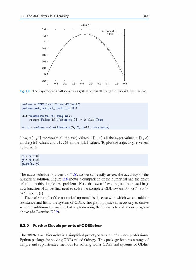
E.3 The ODESolver Class Hierarchy 801
-0.2
0
0.2
0.4
0.6
0.8
1
1.2
1.4
0 0.1 0.2 0.3 0.4 0.5 0.6 0.7 0.8 0.9
dt=0.01
numericalexact
Fig. E.8 The trajectory of a ball solved as a system of four ODEs by the Forward Euler method
solver = ODESolver.ForwardEuler(f)
solver.set_initial_condition(U0)
def terminate(u, t, step_no):
return False if u[step_no,2] >= 0 else True
u, t = solver.solve(linspace(0, T, n+1), terminate)
Now, u[:,0] represents all the x.t/ values, u[:,1] all the vx.t/ values, u[:,2]all the y.t/ values, and u[:,3] all the vy.t/ values. To plot the trajectory, y versusx, we write
x = u[:,0]
y = u[:,2]
plot(x, y)
The exact solution is given by (1.6), so we can easily assess the accuracy of thenumerical solution. Figure E.8 shows a comparison of the numerical and the exactsolution in this simple test problem. Note that even if we are just interested in y
as a function of x, we first need to solve the complete ODE system for x.t/, vx.t/,y.t/, and vy.t/.
The real strength of the numerical approach is the ease with which we can add airresistance and lift to the system of ODEs. Insight in physics is necessary to derivewhat the additional terms are, but implementing the terms is trivial in our programabove (do Exercise E.39).
E.3.9 Further Developments of ODESolver
The ODESolver hierarchy is a simplified prototype version of a more professionalPython package for solving ODEs called Odespy. This package features a range ofsimple and sophisticated methods for solving scalar ODEs and systems of ODEs.
802 E Programming of Differential Equations
Some of the solvers are implemented in Python, while others call up well-knownODE software in Fortran. Like the ODESolver hierarchy, Odespy offers a unifiedinterface to the different numerical methods, which means that the user can spec-ify the ODE problem as a function f(u,t) and send this function to all solvers.This feature makes it easy to switch between solvers to test a wide collection ofnumerical methods for a problem.
Odespy can be downloaded from http://hplgit.github.com/odespy. It isinstalled by the usual python setup.py install command.
E.4 Exercises
Exercise E.1: Solve a simple ODE with function-based codeThis exercise aims to solve the ODE problem u � 10u0 D 0, u.0/ D 0:2, fort 2 Œ0; 20�.
a) Identify the mathematical function f .u; t/ in the generic ODE form u0 Df .u; t/.
b) Implement the f .u; t/ function in a Python function.c) Use the ForwardEuler function from Sect. E.1.3 to compute a numerical solu-
tion of the ODE problem. Use a time step �t D 5.d) Plot the numerical solution and the exact solution u.t/ D 0:2e0:1t .e) Save the numerical solution to file. Decide upon a suitable file format.f) Perform simulations for smaller �t values and demonstrate visually that the
numerical solution approaches the exact solution.
Filename: simple_ODE_func.
Exercise E.2: Solve a simple ODE with class-based codeSolve the same ODE problem as in Exercise E.1, but use the ForwardEuler classfrom Sect. E.1.7. Implement the right-hand side function f as a class too.Filename: simple_ODE_class.
Exercise E.3: Solve a simple ODE with the ODEsolver hierarchySolve the same ODE problem as in Exercise E.1, but use the ForwardEuler classin the ODESolver hierarchy from Sect. E.3.Filename: simple_ODE_class_ODESolver.
Exercise E.4: Solve an ODE specified on the command lineWe want to make a program odesolver_cml.pywhich accepts an ODE problemto be specified on the command line. The command-line arguments are f u0 dt T,where f is the right-hand side f .u; t/ specified as a string formula, u0 is the initialcondition, dt is the time step, and T is the final time of the simulation. A fifth op-tional argument can be given to specify the name of the numerical solution method(set any method of your choice as default value). A curve plot of the solution versustime should be produced and stored in a file plot.png.
E.4 Exercises 803
Hint 1 Use StringFunction from scitools.std for convenient conversion ofa formula on the command line to a Python function.
Hint 2 Use the ODESolver hierarchy to solve the ODE and let the fifth command-line argument be the class name in the ODESolver hierarchy.Filename: odesolver_cml.
Exercise E.5: Implement a numerical method for ODEsImplement the numerical method (E.36)–(E.37). How can you verify that the im-plementation is correct?Filename: Heuns_method.
Exercise E.6: Solve an ODE for emptying a tankA cylindrical tank of radius R is filled with water to a height h0. By opening a valveof radius r at the bottom of the tank, water flows out, and the height of water, h.t/,decreases with time. We can derive an ODE that governs the height function h.t/.
Mass conservation of water requires that the reduction in height balances theoutflow. In a time interval �t , the height is reduced by �h, which corresponds toa water volume of �R2�h. The water leaving the tank in the same interval of timeequals �r2v�t , where v is the outflow velocity. It can be shown (from what isknown as Bernoulli’s equation) [15, 26] that
v.t/ Dp
2gh.t/ C h0.t/2;
where g is the acceleration of gravity. Note that �h > 0 implies an increase inh, which means that ��R2�h is the corresponding decrease in volume that mustbalance the outflow loss of volume �r2v�t . Elimination of v and taking the limit�t ! 0 lead to the ODE
dh
dtD �
� r
R
�2�
1 �� r
R
�4��1=2 p
2gh :
For practical applications r � R so that 1 � .r=R/4 � 1 is a reasonable approx-imation, since other approximations are done as well: friction is neglected in thederivation, and we are going to solve the ODE by approximate numerical methods.The final ODE then becomes
dh
dtD �
� r
R
�2p2gh : (E.61)
The initial condition follows from the initial height of water, h0, in the tank: h.0/ Dh0.
Solve (E.61) by a numerical method of your choice in a program. Set r D 1 cm,R D 20 cm, g D 9:81 m/s2, and h0 D 1 m. Use a time step of 10 seconds. Plotthe solution, and experiment to see what a proper time interval for the simulationis. Make sure to test for h < 0 so that you do not apply the square root function tonegative numbers. Can you find an analytical solution of the problem to comparethe numerical solution with?Filename: tank_ODE.
804 E Programming of Differential Equations
Exercise E.7: Solve an ODE for the arc lengthGiven a curve y D f .x/, the length of the curve from x D x0 to some point x isgiven by the function s.x/, which solves the problem
ds
dxDp
1 C Œf 0.x/�2; s.x0/ D 0 : (E.62)
Since s does not enter the right-hand side, (E.62) can immediately be integratedfrom x0 to x (see Exercise A.13). However, we shall solve (E.62) as an ODE.Use the Forward Euler method and compute the length of a straight line (for easyverification) and a parabola: f .x/ D 1
2x C 1, x 2 Œ0; 2�; f .x/ D x2, x 2 Œ0; 2�.
Filename: arclength_ODE.
Exercise E.8: Simulate a falling or rising body in a fluidA body moving vertically through a fluid (liquid or gas) is subject to three differenttypes of forces:
the gravity force Fg D �mg, where m is the mass of the body and g is theacceleration of gravity;
the drag forceFd D � 12CD%Ajvjv, where CD is a dimensionless drag coefficient
depending on the body’s shape, % is the density of the fluid, A is the cross-sectional area (produced by a cut plane, perpendicular to the motion, through thethickest part of the body), and v is the velocity;
the uplift or buoyancy (“Archimedes”) force Fb D %gV , where V is the volumeof the body.
(Roughly speaking, the Fd formula is suitable for medium to high velocities, whilefor very small velocities, or very small bodies, Fd is proportional to the velocity,not the velocity squared, see [26].)
Newton’s second law applied to the body says that the sum of the listed forcesmust equal the mass of the body times its acceleration a:
Fg C Fd C Fb D ma;
which gives
�mg � 1
2CD%Ajvjv C %gV D ma :
The unknowns here are v and a, i.e., we have two unknowns but only one equation.From kinematics in physics we know that the acceleration is the time derivative ofthe velocity: a D dv=dt . This is our second equation. We can easily eliminate a
and get a single differential equation for v:
�mg � 1
2CD%Ajvjv C %gV D m
dv
dt:
A small rewrite of this equation is handy: we express m as %bV , where %b is thedensity of the body, and we isolate dv=dt on the left-hand side,
dv
dtD �g
�1 � %
%b
�� 1
2CD
%A
%bVjvjv : (E.63)
This differential equation must be accompanied by an initial condition: v.0/ D V0.
E.4 Exercises 805
a) Make a program for solving (E.63) numerically, using any numerical method ofyour choice.
Hint It is not strictly necessary, but it is an elegant Python solution to implement theright-hand side of (E.63) in the __call__method of a class where the parametersg, %, %b, CD , A, and V are data attributes.
b) To verify the program, assume a heavy body in air such that the Fb force can beneglected, and assume a small velocity such that the air resistance Fd can alsobe neglected. Mathematically, setting % D 0 removes both these terms fromthe equation. The solution is then v.t/ D y0.t/ D v0 � gt . Observe throughexperiments that the linear solution is exactly reproduced by the numerical so-lution regardless of the value of �t . (Note that if you use the Forward Eulermethod, the method can become unstable for large �t , see Sect. E.3.5. and timesteps above the critical limit for stability cannot be used to reproduce the linearsolution.) Write a test function for automatically checking that the numericalsolution is uk D v0 � gk�t in this test case.
c) Make a function for plotting the forces Fg , Fb , and Fd as functions of t . See-ing the relative importance of the forces as time develops gives an increasedunderstanding of how the different forces contribute to changing the velocity.
d) Simulate a skydiver in free fall before the parachute opens. We set the densityof the human body as %b D 1003 kg=m3 and the mass as m D 80 kg, implyingV D m=%b D 0:08 m3. We can base the cross-sectional area A the assumptionof a circular cross section of diameter 50 cm, giving A D �R2 D 0:9 m2. Thedensity of air decreases with height, and we here use the value 0.79 kg/m3 whichis relevant for about 5000m height. The CD coefficient can be set as 0.6. Startwith v0 D 0.
e) A ball with the size of a soccer ball is placed in deep water, and we seek to com-pute its motion upwards. Contrary to the former example, where the buoyancyforce Fb is very small, Fb is now the driving force, and the gravity force Fg
is small. Set A D �a2 with a D 11 cm. The mass of the ball is 0.43 kg, thedensity of water is 1000 kg/m3, and CD can be taken as 0.4. Start with v0 D 0.
Filename: body_in_fluid.
Exercise E.9: Verify the limit of a solution as time growsThe solution of (E.63) often tends to a constant velocity, called the terminal veloc-ity. This happens when the sum of the forces, i.e., the right-hand side in (E.63),vanishes.
a) Compute the formula for the terminal velocity by hand.b) Solve the ODE using class ODESolver and call the solve method with
a terminate function that terminates the computations when a constant veloc-ity is reached, that is, when jv.tn/ � v.tn�1/j � �, where � is a small number.
c) Run a series of�t values and make a graph of the terminal velocity as a functionof �t for the two cases in Exercise E.8 d) and e). Indicate the exact terminalvelocity in the plot by a horizontal line.
Filename: body_in_fluid_termvel.
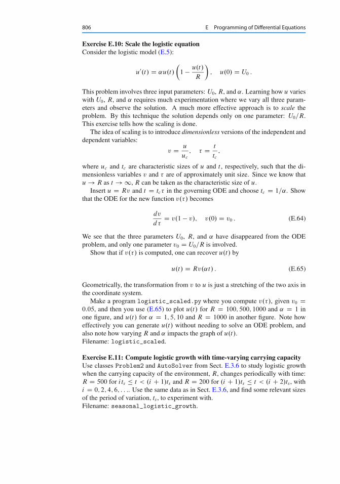
806 E Programming of Differential Equations
Exercise E.10: Scale the logistic equationConsider the logistic model (E.5):
u0.t/ D ˛u.t/
�1 � u.t/
R
�; u.0/ D U0 :
This problem involves three input parameters: U0, R, and ˛. Learning how u varieswith U0, R, and ˛ requires much experimentation where we vary all three param-eters and observe the solution. A much more effective approach is to scale theproblem. By this technique the solution depends only on one parameter: U0=R.This exercise tells how the scaling is done.
The idea of scaling is to introduce dimensionless versions of the independent anddependent variables:
v D u
uc
; � D t
tc;
where uc and tc are characteristic sizes of u and t , respectively, such that the di-mensionless variables v and � are of approximately unit size. Since we know thatu ! R as t ! 1, R can be taken as the characteristic size of u.
Insert u D Rv and t D tc� in the governing ODE and choose tc D 1=˛. Showthat the ODE for the new function v.�/ becomes
dv
d�D v.1 � v/; v.0/ D v0 : (E.64)
We see that the three parameters U0, R, and ˛ have disappeared from the ODEproblem, and only one parameter v0 D U0=R is involved.
Show that if v.�/ is computed, one can recover u.t/ by
u.t/ D Rv.˛t/ : (E.65)
Geometrically, the transformation from v to u is just a stretching of the two axis inthe coordinate system.
Make a program logistic_scaled.py where you compute v.�/, given v0 D0:05, and then you use (E.65) to plot u.t/ for R D 100; 500; 1000 and ˛ D 1 inone figure, and u.t/ for ˛ D 1; 5; 10 and R D 1000 in another figure. Note howeffectively you can generate u.t/ without needing to solve an ODE problem, andalso note how varying R and ˛ impacts the graph of u.t/.Filename: logistic_scaled.
Exercise E.11: Compute logistic growth with time-varying carrying capacityUse classes Problem2 and AutoSolver from Sect. E.3.6 to study logistic growthwhen the carrying capacity of the environment, R, changes periodically with time:R D 500 for i ts � t < .i C 1/ts and R D 200 for .i C 1/ts � t < .i C 2/ts , withi D 0; 2; 4; 6; : : :. Use the same data as in Sect. E.3.6, and find some relevant sizesof the period of variation, ts , to experiment with.Filename: seasonal_logistic_growth.
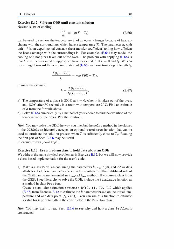
E.4 Exercises 807
Exercise E.12: Solve an ODE until constant solutionNewton’s law of cooling,
dT
dtD �h.T � Ts/ (E.66)
can be used to see how the temperature T of an object changes because of heat ex-change with the surroundings, which have a temperature Ts . The parameter h, withunit s�1 is an experimental constant (heat transfer coefficient) telling how efficientthe heat exchange with the surroundings is. For example, (E.66) may model thecooling of a hot pizza taken out of the oven. The problem with applying (E.66) isthat h must be measured. Suppose we have measured T at t D 0 and t1. We canuse a rough Forward Euler approximation of (E.66) with one time step of length t1,
T .t1/ � T .0/
t1D �h.T .0/ � Ts/;
to make the estimate
h D T .t1/ � T .0/
t1.Ts � T .0//: (E.67)
a) The temperature of a pizza is 200C at t D 0, when it is taken out of the oven,and 180C after 50 seconds, in a room with temperature 20C. Find an estimateof h from the formula above.
b) Solve (E.66) numerically by a method of your choice to find the evolution of thetemperature of the pizza. Plot the solution.
Hint You may solve the ODE the way you like, but the solvemethod in the classesin the ODESolver hierarchy accepts an optional terminate function that can beused to terminate the solution process when T is sufficiently close to Ts . Readingthe first part of Sect. E.3.6 may be useful.Filename: pizza_cooling1.
Exercise E.13: Use a problem class to hold data about an ODEWe address the same physical problem as in Exercise E.12, but we will now providea class-based implementation for the user’s code.
a) Make a class Problem containing the parameters h, Ts , T .0/, and �t as dataattributes. Let these parameters be set in the constructor. The right-hand side ofthe ODE can be implemented in a __call__ method. If you use a class fromthe ODESolver hierarchy to solve the ODE, include the terminate function asa method in class Problem.Create a stand-alone function estimate_h(t0, t1, T0, T1) which applies(E.67) from Exercise E.12 to estimate the h parameter based on the initial tem-perature and one data point .t1; T .t1//. You can use this function to estimatea value for h prior to calling the constructor in the Problem class.
Hint You may want to read Sect. E.3.6 to see why and how a class Problem isconstructed.
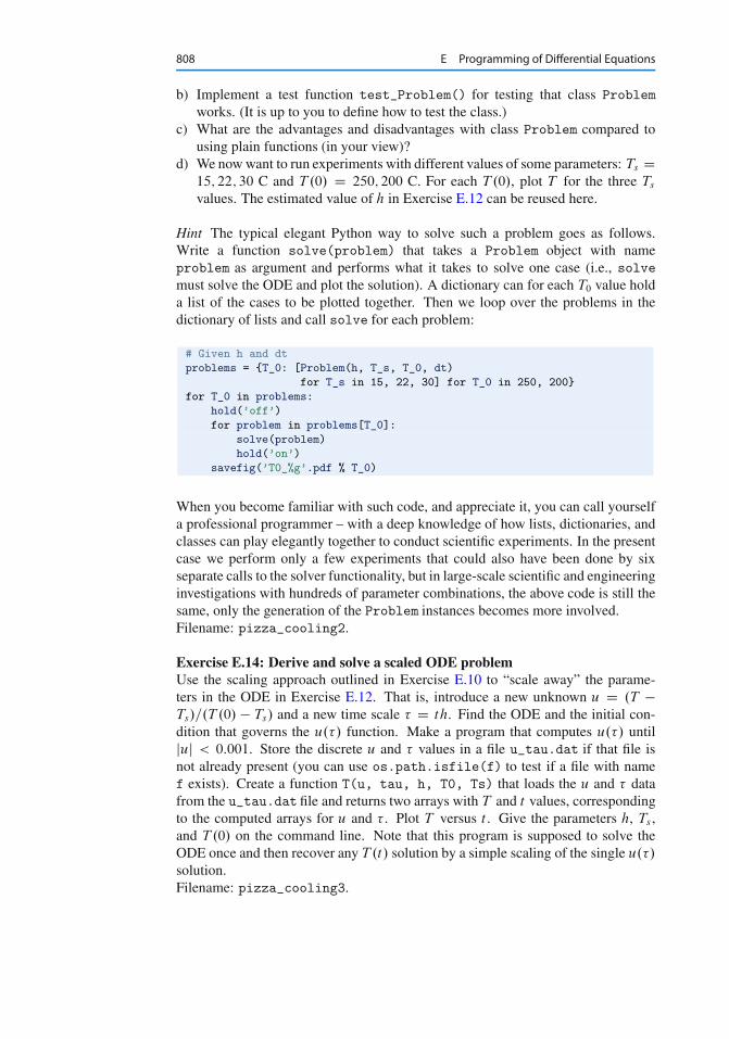
808 E Programming of Differential Equations
b) Implement a test function test_Problem() for testing that class Problemworks. (It is up to you to define how to test the class.)
c) What are the advantages and disadvantages with class Problem compared tousing plain functions (in your view)?
d) We nowwant to run experiments with different values of some parameters: Ts D15; 22; 30 C and T .0/ D 250; 200 C. For each T .0/, plot T for the three Ts
values. The estimated value of h in Exercise E.12 can be reused here.
Hint The typical elegant Python way to solve such a problem goes as follows.Write a function solve(problem) that takes a Problem object with nameproblem as argument and performs what it takes to solve one case (i.e., solvemust solve the ODE and plot the solution). A dictionary can for each T0 value holda list of the cases to be plotted together. Then we loop over the problems in thedictionary of lists and call solve for each problem:
# Given h and dt
problems = {T_0: [Problem(h, T_s, T_0, dt)
for T_s in 15, 22, 30] for T_0 in 250, 200}
for T_0 in problems:
hold(’off’)
for problem in problems[T_0]:
solve(problem)
hold(’on’)
savefig(’T0_%g’.pdf % T_0)
When you become familiar with such code, and appreciate it, you can call yourselfa professional programmer – with a deep knowledge of how lists, dictionaries, andclasses can play elegantly together to conduct scientific experiments. In the presentcase we perform only a few experiments that could also have been done by sixseparate calls to the solver functionality, but in large-scale scientific and engineeringinvestigations with hundreds of parameter combinations, the above code is still thesame, only the generation of the Problem instances becomes more involved.Filename: pizza_cooling2.
Exercise E.14: Derive and solve a scaled ODE problemUse the scaling approach outlined in Exercise E.10 to “scale away” the parame-ters in the ODE in Exercise E.12. That is, introduce a new unknown u D .T �Ts/=.T .0/ � Ts/ and a new time scale � D th. Find the ODE and the initial con-dition that governs the u.�/ function. Make a program that computes u.�/ untiljuj < 0:001. Store the discrete u and � values in a file u_tau.dat if that file isnot already present (you can use os.path.isfile(f) to test if a file with namef exists). Create a function T(u, tau, h, T0, Ts) that loads the u and � datafrom the u_tau.dat file and returns two arrays with T and t values, correspondingto the computed arrays for u and � . Plot T versus t . Give the parameters h, Ts ,and T .0/ on the command line. Note that this program is supposed to solve theODE once and then recover any T .t/ solution by a simple scaling of the single u.�/
solution.Filename: pizza_cooling3.
E.4 Exercises 809
Exercise E.15: Clean up a file to make it a moduleThe ForwardEuler_func.pyfile is not well organized to be used as a module, sayfor doing
>>> from ForwardEuler_func import ForwardEuler
>>> u, t = ForwardEuler(lambda u, t: -u**2, U0=1, T=5, n=30)
The reason is that this import statement will execute a main program in theForwardEuler_func.py file, involving plotting of the solution in an example.Also, the verification tests are run, which in more complicated problems couldtake considerable time and thus make the import statement hang until the tests aredone.
Go through the file and modify it such that it becomes a module where no codeis executed unless the module file is run as a program.Filename: ForwardEuler_func2.
Exercise E.16: Simulate radioactive decayThe equation u0 D �au is a relevant model for radioactive decay, where u.t/ isthe fraction of particles that remains in the radioactive substance at time t . Theparameter a is the inverse of the so-called mean lifetime of the substance. Theinitial condition is u.0/ D 1.
a) Introduce a class Decay to hold information about the physical problem: theparameter a and a __call__method for computing the right-hand side �au ofthe ODE.
b) Initialize an instance of class Decay with a D ln.2/=5600 1/y. The unit 1/ymeans one divided by year, so time is here measured in years, and the particularvalue of a corresponds to the Carbon-14 radioactive isotope whose decay is usedextensively in dating organic material that is tens of thousands of years old.
c) Solve u0 D �au with a time step of 500 y, and simulate the radioactive decay forT D 20; 000 y. Plot the solution. Write out the final u.T / value and compare itwith the exact value e�aT .
Filename: radioactive_decay.
Exercise E.17: Compute inverse functions by solving an ODEThe inverse function g of some function f .x/ takes the value of f .x/ back to x
again: g.f .x// D x. The common technique to compute inverse functions is to sety D f .x/ and solve with respect to x. The formula on the right-hand side is thenthe desired inverse function g.y/. Section A.1.11 makes use of such an approach,where y � f .x/ D 0 is solved numerically with respect to x for different discretevalues of y.
We can formulate a general procedure for computing inverse functions from anODE problem. If we differentiate y D f .x/ with respect to y, we get 1 D f 0.x/dx
dy
by the chain rule. The inverse function we seek is x.y/, but this function thenfulfills the ODE
x0.y/ D 1
f 0.x/: (E.68)
810 E Programming of Differential Equations
That y is the independent coordinate and x a function of y can be a somewhatconfusing notation, so we might introduce u for x and t for y:
u0.t/ D 1
f 0.u/:
The initial condition is x.0/ D xr where xr solves the equation f .xr / D 0 (x.0/
implies y D 0 and then from y D f .x/ it follows that f .x.0// D 0).Make a program that can use the described method to compute the inverse func-
tion of f .x/, given xr . Use any numerical method of your choice for solving theODE problem. Verify the implementation for f .x/ D 2x. Apply the method forf .x/ D p
x and plot f .x/ together with its inverse function.Filename: inverse_ODE.
Exercise E.18: Make a class for computing inverse functionsThe method for computing inverse functions described in Exercise E.17 is verygeneral. The purpose now is to use this general approach to make a more reusableutility, here called Inverse, for computing the inverse of some Python functionf(x) on some interval I=[a,b]. The utility can be used as follows to calculate theinverse of sin x on I D Œ0; �=2�:
def f(x):
return sin(x)
# Compute the inverse of f
inverse = Inverse(f, x0=0, I=[0, pi/2], resolution=100)
x, y = Inverse.compute()
plot(y, x, ’r-’,
x, f(x), ’b-’,
y, asin(y), ’go’)
legend([’computed inverse’, ’f(x)’, ’exact inverse’])
Here, x0 is the value of x at 0, or in general at the left point of the interval: I[0].The parameter resolution tells how many equally sized intervals �y we use inthe numerical integration of the ODE. A default choice of 1000 can be used if it isnot given by the user.
Write class Inverse and put it in a module. Include a test function test_Inverse() in the module for verifying that class Inverse reproduces the exactsolution in the test problem f .x/ D 2x.Filename: Inverse1.
Exercise E.19: Add functionality to a classExtend the module in Exercise E.18 such that the value of x.0/ (x0 in classInverse’s constructor) does not need to be provided by the user.
Hint Class Inverse can compute a value of x.0/ as the root of f .x/ D 0. You mayuse the Bisection method from Sect. 4.11.2, Newton’s method from Sect. A.1.10, orthe Secant method from Exercise A.10 to solve f .x/ D 0. Class Inverse shouldfigure out a suitable initial interval for the Bisection method or start values for the
E.4 Exercises 811
Newton or Secant methods. Computing f .x/ for x at many points and examiningthese may help in solving f .x/ D 0 without any input from the user.Filename: Inverse2.
Exercise E.20: Compute inverse functions by interpolationInstead of solving an ODE for computing the inverse function g.y/ of some func-tion f .x/, as explained in Exercise E.17, one may use a simpler approach based onideas from Sect. E.1.5. Say we compute discrete values of x and f .x/, stored inthe arrays x and y. Doing a plot(x, y) shows y D f .x/ as a function of x, anddoing plot(y, x) shows x as a function of y, i.e., we can trivially plot the inversefunction g.y/ (!).
However, if we want the inverse function of f .x/ as some Python function g(y)that we can call for any y, we can use the tool wrap2callable from Sect. E.1.5to turn the discrete inverse function, described by the arrays y (independent coordi-nate) and x (dependent coordinate), into a continuous function g(y):
from scitools.std import wrap2callable
g = wrap2callable((y, x))
y = 0.5
print g(y)
The g(y) function applies linear interpolation in each interval between the pointsin the y array.
Implement this method in a program. Verify the implementation for f .x/ D 2x,x 2 Œ0; 4�, and apply the method to f .x/ D sin x for x 2 Œ0; �=2�.Filename: inverse_wrap2callable.
Exercise E.21: Code the 4th-order Runge-Kutta method; functionUse the file ForwardEuler_func.py from Sect. E.1.3 as starting point for imple-menting the famous and widely used 4th-order Runge-Kutta method (E.41)–(E.45).Use the test function involving a linear u.t/ for verifying the implementation. Ex-ercise E.23 suggests an application of the code.Filename: RK4_func.
Exercise E.22: Code the 4th-order Runge-Kutta method; classCarry out the steps in Exercise E.21, but base the implementation on the fileForwardEuler.py from Sect. E.1.7.Filename: RK4_class.
Exercise E.23: Compare ODE methodsInvestigate the accuracy of the 4th-order Runge-Kutta method and the Forward Eu-ler scheme for solving the (challenging) ODE problem
dy
dxD 1
2.y � 1/; y.0/ D 1 C p
�; x 2 Œ0; 4�; (E.69)
where � is a small number, say � D 0:001. Start with four steps in Œ0; 4� and reducethe step size repeatedly by a factor of two until you find the solutions sufficiently
812 E Programming of Differential Equations
accurate. Make a plot of the numerical solutions along with the exact solutiony.x/ D 1 C p
x C � for each step size.Filename: yx_ODE_FE_vs_RK4.
Exercise E.24: Code a test function for systems of ODEsThe ForwardEuler_func.py file from Sect. E.1.3 does not contain any test func-tion for verifying the implementation. We can use the fact that linear functions oftime will be exactly reproduced by most numerical methods for ODEs. A simplesystem of two ODEs with linear solutions v.t/ D 2 C 3t and w.t/ D 3 C 4t is
v0 D 3 C .3 C 4t � w/3; (E.70)
w0 D 4 C .2 C 3t � v/4 (E.71)
Write a test function test_ForwardEuler() for comparing the numerical solutionof this system with the exact solution.Filename: ForwardEuler_sys_func2.
Exercise E.25: Code Heun’s method for ODE systems; functionUse the file ForwardEuler_sys_func.py from Sect. E.2.3 as starting point forimplementing Heun’s method (E.36)–(E.37) for systems of ODEs. Verify the solu-tion using the test function suggested in Exercise E.24.Filename: Heun_sys_func.
Exercise E.26: Code Heun’s method for ODE systems; classCarry out the steps in Exercise E.25, but make a class implementation based on thefile ForwardEuler_sys.py from Sect. E.2.4.Filename: Heun_sys_class.
Exercise E.27: Implement and test the Leapfrog method
a) Implement the Leapfrog method specified in formula (E.35) from Sect. E.3.1 ina subclass of ODESolver. Place the code in a separate module file Leapfrog.py.
b) Make a test function for verifying the implementation.
Hint Use the fact that the method will exactly produce a linear u, see Sect. E.3.4.
c) Make a movie that shows how the Leapfrog method, the Forward Euler method,and the 4th-order Runge-Kutta method converge to the exact solution as �t isreduced. Use the model problem u0 D u, u.0/ D 1, t 2 Œ0; 8�, with n D 2k
intervals, k D 1; 2 : : : ; 14. Place the movie generation in a function.d) Repeat c) for the model problem u0 D �u, u.0/ D 1, t 2 Œ0; 5�, with n D 2k
intervals, k D 1; 2 : : : ; 14. In the movie, start with the finest resolution andreduce n until n D 2. The lessons learned is that Leapfrog can give completelywrong, oscillating solutions if the time step is not small enough.
Filename: Leapfrog.
E.4 Exercises 813
Exercise E.28: Implement and test an Adams-Bashforth methodDo Exercise E.27 with the 3rd-order Adams-Bashforth method (E.46).Filename: AdamBashforth3.
Exercise E.29: Solve two coupled ODEs for radioactive decayConsider two radioactive substances A and B. The nuclei in substance A decay toform nuclei of type B with a mean lifetime �A, while substance B decay to formtype A nuclei with a mean lifetime �B . Letting uA and uB be the fractions of theinitial amount of material in substance A and B, respectively, the following systemof ODEs governs the evolution of uA.t/ and uB.t/:
u0A D uB=�B � uA=�A; (E.72)
u0B D uA=�A � uB=�B; (E.73)
with uA.0/ D uB.0/ D 1.
a) Introduce a problem class, which holds the parameters �A and �B and offersa __call__ method to compute the right-hand side vector of the ODE system,i.e., .uB=�B � uA=�A; uA=�A � uB=�B/.
b) Solve for uA and uB using a subclass in the ODESolver hierarchy and the pa-rameter choices �A D 8 minutes, �B D 40 minutes, and �t D 10 seconds.
c) Plot uA and uB against time measured in minutes.d) From the ODE system it follows that the ratio uA=uB ! �A=�B as t ! 1
(assuming u0A D u0
B D 0 in the limit t ! 1). Extend the problem classwith a test method for checking that two given solutions uA and uB fulfill thisrequirement. Verify that this is indeed the case with the computed solutions inb).
Filename: radioactive_decay2.
Exercise E.30: Implement a 2nd-order Runge-Kutta method; functionImplement the 2nd-order Runge-Kutta method specified in formula (E.38). Usea plain function RungeKutta2 of the type shown in Sect. E.1.2 for the ForwardEuler method. Construct a test problem where you know the analytical solution,and plot the difference between the numerical and analytical solution. Demonstratethat the numerical solution approaches the exact solution as �t is reduced.Filename: RungeKutta2_func.
Exercise E.31: Implement a 2nd-order Runge-Kutta method; class
a) Make a new subclass RungeKutta2 in the ODESolver hierarchy from Sect. E.3for solving ordinary differential equations with the 2nd-order Runge-Kuttamethod specified in formula (E.38).
b) Construct a test problemwhere you can find an exact solution. Run different val-ues of �t and demonstrate in a plot that the numerical solution approaches theexact solution as �t is decreased. Put the code that creates the plot in a function.
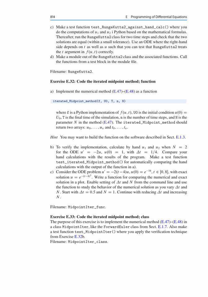
814 E Programming of Differential Equations
c) Make a test function test_RungeKutta2_against_hand_calc()where youdo the computations of u1 and u2 i Python based on the mathematical formulas.Thereafter, run the RungeKutta2 class for two time steps and check that the twosolutions are equal (within a small tolerance). Use an ODE where the right-handside depends on t as well as u such that you can test that RungeKutta2 treatsthe t argument in f .u; t/ correctly.
d) Make a module out of the RungeKutta2 class and the associated functions. Callthe functions from a test block in the module file.
Filename: RungeKutta2.
Exercise E.32: Code the iterated midpoint method; function
a) Implement the numerical method (E.47)–(E.48) as a function
iterated_Midpoint_method(f, U0, T, n, N)
where f is a Python implementation of f .u; t/, U0 is the initial condition u.0/ DU0, T is the final time of the simulation, n is the number of time steps, and N is theparameter N in the method (E.47). The iterated_Midpoint_method shouldreturn two arrays: u0; : : : ; un and t0; : : : ; tn.
Hint You may want to build the function on the software described in Sect. E.1.3.
b) To verify the implementation, calculate by hand u1 and u2 when N D 2
for the ODE u0 D �2u, u.0/ D 1, with �t D 1=4. Compare yourhand calculations with the results of the program. Make a test functiontest_iterated_Midpoint_method() for automatically comparing the handcalculations with the output of the function in a).
c) Consider the ODE problem u0 D �2.t �4/u, u.0/ D e�16, t 2 Œ0; 8�, with exactsolution u D e�.t�4/2
. Write a function for comparing the numerical and exactsolution in a plot. Enable setting of �t and N from the command line and usethe function to study the behavior of the numerical solution as you vary �t andN . Start with �t D 0:5 and N D 1. Continue with reducing �t and increasingN .
Filename: MidpointIter_func.
Exercise E.33: Code the iterated midpoint method; classThe purpose of this exercise is to implement the numerical method (E.47)–(E.48) ina class MidpointIter, like the ForwardEuler class from Sect. E.1.7. Also makea test function test_MidpointIter()where you apply the verification techniquefrom Exercise E.32b.Filename: MidpointIter_class.
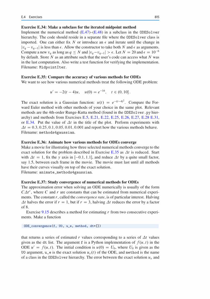
E.4 Exercises 815
Exercise E.34: Make a subclass for the iterated midpoint methodImplement the numerical method (E.47)–(E.48) in a subclass in the ODESolverhierarchy. The code should reside in a separate file where the ODESolver class isimported. One can either fix N or introduce an � and iterate until the change injvq � vq�1j is less than �. Allow the constructor to take both N and � as arguments.Compute a new vq as long as q � N and jvq �vq�1j > �. Let N D 20 and � D 10�6
by default. Store N as an attribute such that the user’s code can access what N wasin the last computation. Also write a test function for verifying the implementation.Filename: MidpointIter.
Exercise E.35: Compare the accuracy of various methods for ODEsWe want to see how various numerical methods treat the following ODE problem:
u0 D �2.t � 4/u; u.0/ D e�16; t 2 .0; 10� :
The exact solution is a Gaussian function: u.t/ D e�.t�4/2. Compare the For-
ward Euler method with other methods of your choice in the same plot. Relevantmethods are the 4th-order Runge-Kutta method (found in the ODESolver.py hier-archy) and methods from Exercises E.5, E.21, E.22, E.25, E.26, E.27, E.28 E.31,or E.34. Put the value of �t in the title of the plot. Perform experiments with�t D 0:3; 0:25; 0:1; 0:05; 0:01; 0:001 and report how the various methods behave.Filename: methods4gaussian.
Exercise E.36: Animate how various methods for ODEs convergeMake a movie for illustrating how three selected numerical methods converge to theexact solution for the problem described in Exercise E.35 as �t is reduced. Startwith �t D 1, fix the y axis in Œ�0:1; 1:1�, and reduce �t by a quite small factor,say 1.5, between each frame in the movie. The movie must last until all methodshave their curves visually on top of the exact solution.Filename: animate_methods4gaussian.
Exercise E.37: Study convergence of numerical methods for ODEsThe approximation error when solving an ODE numerically is usually of the formC�tr , where C and r are constants that can be estimated from numerical experi-ments. The constant r , called the convergence rate, is of particular interest. Halving�t halves the error if r D 1, but if r D 3, halving �t reduces the error by a factorof 8.
Exercise 9.15 describes a method for estimating r from two consecutive experi-ments. Make a function
ODE_convergence(f, U0, u_e, method, dt=[])
that returns a series of estimated r values corresponding to a series of �t valuesgiven as the dt list. The argument f is a Python implementation of f .u; t/ in theODE u0 D f .u; t/. The initial condition is u.0/ D U0, where U0 is given as theU0 argument, u_e is the exact solution ue.t/ of the ODE, and method is the nameof a class in the ODESolver hierarchy. The error between the exact solution ue and
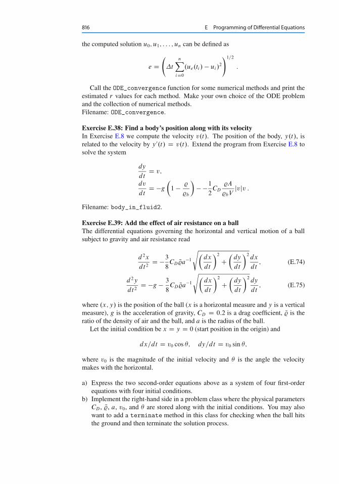
816 E Programming of Differential Equations
the computed solution u0; u1; : : : ; un can be defined as
e D
�t
nXiD0
.ue.ti / � ui/2
!1=2
:
Call the ODE_convergence function for some numerical methods and print theestimated r values for each method. Make your own choice of the ODE problemand the collection of numerical methods.Filename: ODE_convergence.
Exercise E.38: Find a body’s position along with its velocityIn Exercise E.8 we compute the velocity v.t/. The position of the body, y.t/, isrelated to the velocity by y0.t/ D v.t/. Extend the program from Exercise E.8 tosolve the system
dy
dtD v;
dv
dtD �g
�1 � %
%b
�� �1
2CD
%A
%bVjvjv :
Filename: body_in_fluid2.
Exercise E.39: Add the effect of air resistance on a ballThe differential equations governing the horizontal and vertical motion of a ballsubject to gravity and air resistance read
d 2x
dt2D �3
8CD N%a�1
s�dx
dt
�2
C�
dy
dt
�2dx
dt; (E.74)
d 2y
dt2D �g � 3
8CD N%a�1
s�dx
dt
�2
C�
dy
dt
�2dy
dt; (E.75)
where .x; y/ is the position of the ball (x is a horizontal measure and y is a verticalmeasure), g is the acceleration of gravity, CD D 0:2 is a drag coefficient, N% is theratio of the density of air and the ball, and a is the radius of the ball.
Let the initial condition be x D y D 0 (start position in the origin) and
dx=dt D v0 cos ; dy=dt D v0 sin ;
where v0 is the magnitude of the initial velocity and is the angle the velocitymakes with the horizontal.
a) Express the two second-order equations above as a system of four first-orderequations with four initial conditions.
b) Implement the right-hand side in a problem class where the physical parametersCD , N%, a, v0, and are stored along with the initial conditions. You may alsowant to add a terminate method in this class for checking when the ball hitsthe ground and then terminate the solution process.
E.4 Exercises 817
c) Simulate a hard football kick where v0 D 120 km/h and is 30 degrees. Takethe density of the ball as 0.017 hg=m3 and the radius as 11 cm. Solve the ODEsystem for CD D 0 (no air resistance) and CD D 0:2, and plot y as a function ofx in both cases to illustrate the effect of air resistance. Make sure you expressall units in kg, m, s, and radians.
Filename: kick2D.
Exercise E.40: Solve an ODE system for an electric circuitAn electric circuit with a resistor, a capacitor, an inductor, and a voltage source canbe described by the ODE
LdI
dtC RI C Q
CD E.t/; (E.76)
where LdI=dt is the voltage drop across the inductor, I is the current (measuredin amperes, A), L is the inductance (measured in henrys, H), R is the resistance(measured in ohms, ˝), Q is the charge on the capacitor (measured in coulombs,C), C is the capacitance (measured in farads, F), E.t/ is the time-variable voltagesource (measured in volts, V), and t is time (measured in seconds, s). There isa relation between I and Q:
dQ
dtD I : (E.77)
Equations (E.76)–(E.77) is a system two ODEs. Solve these for L D 1 H, E.t/ D2 sin!t V, !2 D 3:5 s�2, C D 0:25 C, R D 0:2 ˝, I.0/ D 1 A, and Q.0/ D 1C .Use the Forward Euler scheme with �t D 2�=.60!/. The solution will, after sometime, oscillate with the same period as E.t/, a period of 2�=!. Simulate 10 periods.Filename: electric_circuit.
Remarks It turns out that the Forward Euler scheme overestimates the amplitudesof the oscillations. The more accurate 4th-order Runge-Kutta method is much betterfor this type of differential equation model.
Exercise E.41: Simulate the spreading of a disease by a SIR modelWe shall in this exercise model epidemiological diseases such as measles or swineflu. Suppose we have three categories of people: susceptibles (S) who can get thedisease, infected (I) who have developed the disease and who can infect suscepti-bles, and recovered (R) who have recovered from the disease and become immune.Let S.t/, I.t/, and R.t/ be the number of people in category S, I, and R, respec-tively. We have that S CI CR D N , where N is the size of the population, assumedconstant here for simplicity.
When people mix in the population there are SI possible pairs of susceptiblesand infected, and a certain fraction ˇSI per time interval meets with the resultthat the infected “successfully” infect the susceptible. During a time interval �t ,ˇSI�t get infected and move from the S to the I category:
S.t C �t/ D S.t/ � ˇSI�t :
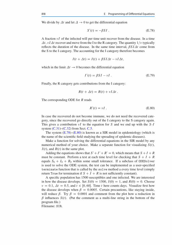
818 E Programming of Differential Equations
We divide by �t and let � ! 0 to get the differential equation
S 0.t/ D �ˇSI : (E.78)
A fraction �I of the infected will per time unit recover from the disease. In a time�t , �I�t recover and move from the I to the R category. The quantity 1=� typicallyreflects the duration of the disease. In the same time interval, ˇSI�t come fromthe S to the I category. The accounting for the I category therefore becomes
I.t C �t/ D I.t/ C ˇSI�t � �I�t;
which in the limit �t ! 0 becomes the differential equation
I 0.t/ D ˇSI � �I : (E.79)
Finally, the R category gets contributions from the I category:
R.t C �t/ D R.t/ C �I�t :
The corresponding ODE for R reads
R0.t/ D �I : (E.80)
In case the recovered do not become immune, we do not need the recovered cate-gory, since the recovered go directly out of the I category to the S category again.This gives a contribution �I to the equation for S and we end up with the S-Isystem (C.31)–(C.32) from Sect. C.5.
The system (E.78)–(E.80) is known as a SIR model in epidemiology (which isthe name of the scientific field studying the spreading of epidemic diseases).
Make a function for solving the differential equations in the SIR model by anynumerical method of your choice. Make a separate function for visualizing S.t/,I.t/, and R.t/ in the same plot.
Adding the equations shows that S 0 CI 0 CR0 D 0, which means that S CI CR
must be constant. Perform a test at each time level for checking that S C I C R
equals S0 C I0 C R0 within some small tolerance. If a subclass of ODESolveris used to solve the ODE system, the test can be implemented as a user-specifiedterminate function that is called by the solvemethod a every time level (simplyreturn True for termination if S C I C R is not sufficiently constant).
A specific population has 1500 susceptibles and one infected. We are interestedin how the disease develops. Set S.0/ D 1500, I.0/ D 1, and R.0/ D 0. Choose� D 0:1, �t D 0:5, and t 2 Œ0; 60�. Time t here counts days. Visualize first howthe disease develops when ˇ D 0:0005. Certain precautions, like staying inside,will reduce ˇ. Try ˇ D 0:0001 and comment from the plot how a reduction inˇ influences S.t/. (Put the comment as a multi-line string in the bottom of theprogram file.)Filename: SIR.
E.4 Exercises 819
Exercise E.42: Introduce problem and solver classes in the SIR modelThe parameters � and ˇ in the SIR model in Exercise E.41 can be constants orfunctions of time. Now we shall make an implementation of the f .u; t/ functionspecifying the ODE system such that � and ˇ can be given as either a constant ora Python function. Introduce a class for f .u; t/, with the following code sketch:
class ProblemSIR(object):
def __init__(self, nu, beta, S0, I0, R0, T):
"""
nu, beta: parameters in the ODE system
S0, I0, R0: initial values
T: simulation for t in [0,T]
"""
if isinstance(nu, (float,int)): # number?
self.nu = lambda t: nu # wrap as function
elif callable(nu):
self.nu = nu
# same for beta and self.beta
...
# store the other parameters
def __call__(self, u, t):
"""Right-hand side function of the ODE system."""
S, I, R = u
return [-self.beta(t)*S*I, # S equation
..., # I equation
self.nu(t)*I] # R equation
# Example:
problem = ProblemSIR(beta=lambda t: 0.0005 if t <= 12 else 0.0001,
nu=0.1, S0=1500, I0=1, R0=0, T=60)
solver = ODESolver.ForwardEuler(problem)
Write the complete code for class ProblemSIR based on the sketch of ideas above.The � parameter is usually not varying with time as 1=� is a characteristic size ofthe period a person is sick, but introduction of new medicine during the diseasemight change the picture such that time dependence becomes relevant.
We can also make a class SolverSIR for solving the problem (see Sect. E.3.6for similar examples):
class SolverSIR(object):
def __init__(self, problem, dt):
self.problem, self.dt = problem, dt
def solve(self, method=ODESolver.RungeKutta4):
self.solver = method(self.problem)
ic = [self.problem.S0, self.problem.I0, self.problem.R0]
self.solver.set_initial_condition(ic)
n = int(round(self.problem.T/float(self.dt)))
t = np.linspace(0, self.problem.T, n+1)
820 E Programming of Differential Equations
u, self.t = self.solver.solve(t)
self.S, self.I, self.R = u[:,0], u[:,1], u[:,2]
def plot(self):
# plot S(t), I(t), and R(t)
After the breakout of a disease, authorities often start campaigns for decreas-ing the spreading of the disease. Suppose a massive campaign telling people towash their hands more frequently is launched, with the effect that ˇ is significantlyreduced after some days. For the specific case simulated in Exercise E.41, let
ˇ.t/ D(
0:0005; 0 � t � 12;
0:0001; t > 12
Simulate this scenario with the Problem and Solver classes. Report the maximumnumber of infected people and compare it to the case where ˇ.t/ D 0:0005.Filename: SIR_class.
Exercise E.43: Introduce vaccination in a SIR modelWe shall now extend the SIR model in Exercise E.41 with a vaccination2 program.If a fraction p of the susceptibles per time unit is being vaccinated, and we say thatthe vaccination is 100 percent effective, pS�t individuals will be removed from theS category in a time interval �t . We place the vaccinated people in a new categoryV. The equations for S and V becomes
S 0 D �ˇSI � pS; (E.81)
V 0 D pS : (E.82)
The equations for I and R are not affected. The initial condition for V can be takenas V.0/ D 0. The resulting model is named SIRV.
Try the same parameters as in Exercise E.41 in combination with p D 0:1 andcompute the evolution of S.t/, I.t/, R.t/, and V.t/. Comment on the effect ofvaccination on the maximum number of infected.
Hint You can of course edit the code from Exercise E.42, but it is much betterto avoid duplicating code and use object-oriented programming to implement theextensions in the present exercise as subclasses of the classes from Exercise E.42.Filename: SIRV.
Exercise E.44: Introduce a vaccination campaign in a SIR modelLet the vaccination campaign in Exercise E.43 start 6 days after the outbreak of thedisease and let it last for 10 days,
p.t/ D(
0:1; 6 � t � 15;
0; otherwise
2 https://www.youtube.com/watch?v=s_6QW9sNPEY
E.4 Exercises 821
Plot the corresponding solutions S.t/, I.t/, R.t/, and V.t/. (It is clearly advan-tageous to have the SIRV model implemented as an extension to the classes inExercise E.42.)Filename: SIRV_varying_p.
Exercise E.45: Find an optimal vaccination periodLet the vaccination campaign in Exercise E.44 last for VT days:
p.t/ D(
0:1; 6 � t � 6 C VT ;
0; otherwise
Compute the maximum number of infected people, maxt I.t/, as a function of VT 2Œ0; 31�, by running the model for VT D 0; 1; 2 : : : ; 31. Plot this function. Determinefrom the plot the optimal VT , i.e., the smallest vaccination period VT such thatincreasing VT has negligible effect on the maximum number of infected people.Filename: SIRV_optimal_duration.
Exercise E.46: Simulate human-zombie interactionSuppose the human population is attacked by zombies. This is quite a common hap-pening in movies, and the “zombification” of humans acts much like the spreadingof a disease. Let us make a differential equation model, inspired by the SIR modelfrom Exercise E.41, to simulate how humans and zombies interact.
We introduce four categories of individuals:
1. S: susceptible humans who can become zombies.2. I: infected humans, being bitten by zombies.3. Z: zombies.4. R: removed individuals, either conquered zombies or dead humans.
The corresponding functions counting how many individuals we have in each cate-gory are named S.t/, I.t/, Z.t/, and R.t/, respectively.
The type of zombies considered here is inspired by the standard for modern zom-bies set by the classic movie The Night of the Living Dead, by George A. Romerofrom 1968. Only a small extension of the SIR model is necessary to model theeffect of human-zombie interaction mathematically. A fraction of the human sus-ceptibles is getting bitten by zombies and moves to the infected category. A fractionof the infected is then turned into zombies. On the other hand, humans can conquerzombies.
Now we shall precisely set up all the dynamic features of the human-zombiepopulations we aim to model. Changes in the S category are due to three effects:
1. Susceptibles are infected by zombies, modeled by a term ��tˇSZ, similar tothe S-I interaction in the SIR model.
2. Susceptibles die naturally or get killed and therefore enter the removed category.If the probability that one susceptible dies during a unit time interval is ıS , thetotal expected number of deaths in a time interval �t becomes �tıS S .
822 E Programming of Differential Equations
3. We also allow new humans to enter the area with zombies, as this effect may benecessary to successfully run a war on zombies. The number of new individualsin the S category arriving per time unit is denoted by ˙ , giving an increase inS.t/ by �t˙ during a time �t .
We could also add newborns to the S category, but we simply skip this effect sinceit will not be significant over time scales of a few days.
The balance of the S category is then
S 0 D ˙ � ˇSZ � ıS S;
in the limit �t ! 0.The infected category gets a contribution �tˇSZ from the S category, but loses
individuals to the Z and R category. That is, some infected are turned into zombies,while others die. Movies reveal that infected may commit suicide or that others(susceptibles) may kill them. Let ıI be the probability of being killed in a unit timeinterval. During time �t , a total of ıI �tI will die and hence be transferred to theremoved category. The probability that a single infected is turned into a zombieduring a unit time interval is denoted by �, so that a total of �t�I individuals arelost from the I to the Z category in time �t . The accounting in the I categorybecomes
I 0 D ˇSZ � �I � ıI I :
The zombie category gains ��t�I individuals from the I category. We disregardthe effect that any removed individual can turn into a zombie again, as we considerthat effect as pure magic beyond reasonable behavior, at least according to what isobserved in the Romero movie tradition. A fundamental feature in zombie moviesis that humans can conquer zombies. Here we consider zombie killing in a “man-to-man” human-zombie fight. This interaction resembles the nature of zombification(or the susceptible-infective interaction in the SIR model) and can be modeled bya loss �˛SZ for some parameter ˛ with an interpretation similar to that of ˇ. Theequation for Z then becomes
Z 0 D �I � ˛SZ :
The accounting in the R category consists of a gain ıS of natural deaths from theS category, a gain ıI from the I category, and a gain ˛SZ from defeated zombies:
R0 D ıSS C ıI I C ˛SZ :
The complete SIZR model for human-zombie interaction can be summarized as
S 0 D ˙ � ˇSZ � ıS S; (E.83)
I 0 D ˇSZ � �I � ıI I; (E.84)
Z 0 D �I � ˛SZ; (E.85)
R0 D ıS S C ıI I C ˛SZ : (E.86)
E.4 Exercises 823
The interpretations of the parameters are as follows:
˙ : the number of new humans brought into the zombified area per unit time. ˇ: the probability that a theoretically possible human-zombie pair actually meets
physically, during a unit time interval, with the result that the human is infected. ıS : the probability that a susceptible human is killed or dies, in a unit time
interval. ıI : the probability that an infected human is killed or dies, in a unit time interval. �: the probability that an infected human is turned into a zombie, during a unit
time interval. ˛: the probability that, during a unit time interval, a theoretically possible
human-zombie pair fights and the human kills the zombie.
Note that probabilities per unit time do not necessarily lie in the interval Œ0; 1�.The real probability, lying between 0 and 1, arises after multiplication by the timeinterval of interest.
Implement the SIZR model with a Problem and Solver class as explained inExercise E.42, allowing parameters to vary in time. The time variation is essentialto make a realistic model that can mimic what happens in movies.
Test the implementation with the following data: ˇ D 0:0012, ˛ D 0:0016,ıI D 0:014, ˙ D 2, � D 1, S.0/ D 10, Z.0/ D 100, I.0/ D 0, R.0/ D 0, andsimulation time T D 24 hours. Other parameters can be set to zero. These valuesare estimated from the hysterical phase of the movie The Night of the Living Dead.The time unit is hours. Plot the S , I , Z, and R quantities.Filename: SIZR.
Exercise E.47: Simulate a zombie movieThe movie The Night of the Living Dead has three phases:
1. The initial phase, lasting for (say) 4 hours, where two humans meet one zombieand one of the humans get infected. A rough (and uncertain) estimation ofparameters in this phase, taking into account dynamics not shown in the movie,yet necessary to establish a more realistic evolution of the S and Z categorieslater in the movie, is ˙ D 20, ˇ D 0:03, � D 1, S.0/ D 60, and Z.0/ D 1. Allother parameters are taken as zero when not specified.
2. The hysterical phase, when the zombie treat is evident. This phase lasts for24 hours, and relevant parameters can be taken as ˇ D 0:0012, ˛ D 0:0016,ıI D 0:014, ˙ D 2, � D 1.
3. The counter attack by humans, estimated to last for 5 hours, with parameters˛ D 0:006, ˇ D 0 (humans no longer get infected), ıS D 0:0067, � D 1.
Use the program from Exercise E.46 to simulate all three phases of the movie.
Hint It becomes necessary to work with piecewise constant functions in time.These can be hardcoded for each special case, our one can employ a ready-madetool for such functions (actually developed in Exercise 3.32):
824 E Programming of Differential Equations
from scitools.std import PiecewiseConstant
# Define f(t) as 1.5 in [0,3], 0.1 in [3,4] and 1 in [4,7]
f = PiecewiseConstant(domain=[0, 7],
data=[(0, 1.5), (3, 0.1), (4, 1)])
Filename: Night_of_the_Living_Dead.
Exercise E.48: Simulate a war on zombiesAwar on zombies can be implemented through large-scale effective attacks. A pos-sible model is to increase ˛ in the SIZR model from Exercise E.46 by some ad-ditional amount !.t/, where !.t/ varies in time to model strong attacks at m C 1
distinct points of time T0 < T1 < � � � < Tm. Around these t values we want ! tohave a large value, while in between the attacks ! is small. One possible mathe-matical function with this behavior is a sum of Gaussian functions:
!.t/ D a
mXiD0
exp
�1
2
�t � Ti
�2!
; (E.87)
where a measures the strength of the attacks (the maximum value of !.t/) and measures the length of the attacks, which should be much less than the timebetween the points of attack: typically, 4 measures the length of an attack, and wemust have 4 � Ti � Ti�1 for i D 1; : : : ; m. We should choose a significantlylarger than ˛ to make the attacks in the war on zombies much stronger than theusual “man-to-man” killing of zombies.
Modify the model and the implementation from Exercise E.46 to include a waron zombies. We start out with 50 humans and 3 zombies and ˇ D 0:03. Thisleads to rapid zombification. Assume that there are some small resistances againstzombies from the humans, ˛ D 0:2ˇ, throughout the simulations. In addition, thehumans implement three strong attacks, a D 50˛, at 5, 10, and 18 hours after thezombification starts. The attacks last for about 2 hours ( D 0:5). Set ıS D �I D˙ D 0, ˇ D 0:03, and � D 1, simulate for T D 20 hours, and see if the war onzombies modeled by the suggested !.t/ is sufficient to save mankind.Filename: war_on_zombies.
Exercise E.49: Explore predator-prey population interactionsSuppose we have two species in an environment: a predator and a prey. Howwill thetwo populations interact and change with time? A system of ordinary differentialequations can give insight into this question. Let x.t/ and y.t/ be the size of theprey and the predator populations, respectively. In the absence of a predator, thepopulation of the prey will follow the ODE derived in Sect. C.2:
dx
dtD rx;
with r > 0, assuming there are enough resources for exponential growth. Similarly,in the absence of prey, the predator population will just experience a death ratem > 0:
dy
dtD �my :
E.4 Exercises 825
In the presence of the predator, the prey population will experience a reduction inthe growth proportional to xy. The number of interactions (meetings) between x
and y numbers of animals is xy, and in a certain fraction of these interactions thepredator eats the prey. The predator population will correspondingly experiencea growth in the population because of the xy interactions with the prey population.The adjusted growth of both populations can now be expressed as
dx
dtD rx � axy; (E.88)
dy
dtD �my C bxy; (E.89)
for positive constants r , m, a, and b. Solve this system and plot x.t/ and y.t/ forr D m D 1, a D 0:3, b D 0:2, x.0/ D 1, and y.0/ D 1, t 2 Œ0; 20�. Try to explainthe dynamics of the population growth you observe. Experiment with other valuesof a and b.Filename: predator_prey.
Exercise E.50: Formulate a 2nd-order ODE as a systemIn this and subsequent exercises we shall deal with the following second-order or-dinary differential equation with two initial conditions:
m Ru C f . Pu/ C s.u/ D F.t/; t > 0; u.0/ D U0; Pu.0/ D V0 : (E.90)
The notation Pu and Ru means u0.t/ and u00.t/, respectively. Write (E.90) as a systemof two first-order differential equations. Also set up the initial condition for thissystem.
Physical applications Equation (E.90) has a wide range of applications throughoutscience and engineering. A primary application is damped spring systems in, e.g.,cars and bicycles: u is the vertical displacement of the spring system attached toa wheel; Pu is then the corresponding velocity; F.t/ resembles a bumpy road; s.u/
represents the force from the spring; and f . Pu/ models the damping force (friction)in the spring system. For this particular application f and s will normally be linearfunctions of their arguments: f . Pu/ D ˇ Pu and s.u/ D ku, where k is a springconstant and ˇ some parameter describing viscous damping.
Equation (E.90) can also be used to describe the motions of a moored ship oroil platform in waves: the moorings act as a nonlinear spring s.u/; F.t/ representsenvironmental excitation from waves, wind, and current; f . Pu/ models damping ofthe motion; and u is the one-dimensional displacement of the ship or platform.
Oscillations of a pendulum can be described by (E.90): u is the angle the pendu-lum makes with the vertical; s.u/ D .mg=L/ sin.u/, where L is the length of thependulum,m is the mass, and g is the acceleration of gravity; f . Pu/ D ˇj Puj Pu modelsair resistance (with ˇ being some suitable constant, see Exercises 1.11 and E.54);and F.t/ might be some motion of the top point of the pendulum.
Another application is electric circuits with u.t/ as the charge, m D L as theinductance, f . Pu/ D R Pu as the voltage drop across a resistor R, s.u/ D u=C as thevoltage drop across a capacitor C , and F.t/ as an electromotive force (supplied bya battery or generator).
826 E Programming of Differential Equations
Furthermore, Equation (E.90) can act as a (very) simplified model of many otheroscillating systems: aircraft wings, lasers, loudspeakers, microphones, tuning forks,guitar strings, ultrasound imaging, voice, tides, the El Ni no phenomenon, climatechanges – to mention some.
We remark that (E.90) is a possibly nonlinear generalization of Equation (D.8)explained in Sect. D.1.3. The case in Appendix D corresponds to the special choiceof f . Pu/ proportional to the velocity Pu, s.u/ proportional to the displacement u, andF.t/ as the acceleration Rw of the plate and the action of the gravity force.
Exercise E.51: Solve Ru C u D 0
Make a function
def rhs(u, t):
...
for returning a list with two elements with the two right-hand side expressions inthe first-order differential equation system from Exercise E.50. As usual, the u ar-gument is an array or list with the two solution components u[0] and u[1] at sometime t. Inside rhs, assume that you have access to three global Python functionsfriction(dudt), spring(u), and external(t) for evaluating f . Pu/, s.u/, andF.t/, respectively.
Test the rhs function in combination with the functions f . Pu/ D 0, F.t/ D0, s.u/ D u, and the choice m D 1. The differential equation then reads Ru Cu D 0. With initial conditions u.0/ D 1 and Pu.0/ D 0, one can show that thesolution is given by u.t/ D cos.t/. Apply three numerical methods: the 4th-orderRunge-Kutta method and the Forward Euler method from the ODESolver moduledeveloped in Sect. E.3, as well as the 2nd-order Runge-Kutta method developed inExercise E.31. Use a time step �t D �=20.
Plot u.t/ and Pu.t/ versus t together with the exact solutions. Also make a plotof Pu versus u (plot(u[:,0], u[:,1]) if u is the array returned from the solver’ssolve method). In the latter case, the exact plot should be a circle because thepoints on the curve are .cos t; sin t/, which all lie on a circle as t is varied. Ob-serve that the ForwardEuler method results in a spiral and investigate how the spiraldevelops as �t is reduced.
The kinetic energy K of the motion is given by 12m Pu2, and the potential en-
ergy P (stored in the spring) is given by the work done by the spring force: P DR u
0s.v/dv D 1
2u2. Make a plot with K and P as functions of time for both the
4th-order Runge-Kutta method and the Forward Euler method, for the same physi-cal problem described above. In this test case, the sum of the kinetic and potentialenergy should be constant. Compute this constant analytically and plot it togetherwith the sum K C P as calculated by the 4th-order Runge-Kutta method and theForward Euler method.Filename: oscillator_v1.
Exercise E.52: Make a tool for analyzing oscillatory solutionsThe solution u.t/ of the equation (E.90) often exhibits an oscillatory behavior (forthe test problem in Exercise E.51 we have that u.t/ D cos t). It is then of interestto find the wavelength of the oscillations. The purpose of this exercise is to find and
E.4 Exercises 827
visualize the distance between peaks in a numerical representation of a continuousfunction.
Given an array .y0; : : : ; yn�1/ representing a function y.t/ sampled at variouspoints t0; : : : ; tn�1, a local maximum of y.t/ occurs at t D tk if yk�1 < yk > ykC1.Similarly, a local minimum of y.t/ occurs at t D tk if yk�1 > yk < ykC1. Byiterating over the y1; : : : ; yn�2 values and making the two tests, one can collectlocal maxima and minima as .tk; yk/ pairs. Make a function minmax(t, y) whichreturns two lists, minima and maxima, where each list holds pairs (2-tuples) of t andy values of local minima or maxima. Ensure that the t value increases from one pairto the next. The arguments t and y in minmax hold the coordinates t0; : : : ; tn�1 andy0; : : : ; yn�1, respectively.
Make another function wavelength(peaks) which takes a list peaks of2-tuples with t and y values for local minima or maxima as argument and re-turns an array of distances between consecutive t values, i.e., the distancesbetween the peaks. These distances reflect the local wavelength of the com-puted y function. More precisely, the first element in the returned array ispeaks[1][0]-peaks[0][0], the next element is peaks[2][0]-peaks[1][0],and so forth.
Test the minmax and wavelength functions on y values generated by y Det=4 cos.2t/ and y D e�t=4 cos.t2=5/ for t 2 Œ0; 4��. Plot the y.t/ curve in eachcase, and mark the local minima and maxima computed by minmax with circlesand boxes, respectively. Make a separate plot with the array returned from thewavelength function (just plot the array against its indices – the point is to see ifthe wavelength varies or not). Plot only the wavelengths corresponding to maxima.
Make a module with the minmax and wavelength function, and let the test blockperform the tests specified above.Filename: wavelength.
Exercise E.53: Implement problem, solver, and visualizer classesThe user-chosen functions f , s, and F in Exercise E.51 must be coded with par-ticular names. It is then difficult to have several functions for s.u/ and experimentwith these. A much more flexible code arises if we adopt the ideas of a problemand a solver class as explained in Sect. E.3.6. Specifically, we shall here make useof class Problem3 in Sect. E.3.6 to store information about f . Pu/, s.u/, F.t/, u.0/,Pu.0/, m, T , and the exact solution (if available). The solver class can store param-eters related to the numerical quality of the solution, i.e., �t and the name of thesolver class in the ODESolver hierarchy. In addition we will make a visualizer classfor producing plots of various kinds.
We want all parameters to be set on the command line, but also have sensibledefault values. As in Sect. E.3.6, the argparse module is used to read data fromthe command line. Class Problem can be sketched as follows:
class Problem(object):
def define_command_line_arguments(self, parser):
"""Add arguments to parser (argparse.ArgumentParser)."""
parser.add_argument(
’--friction’, type=func_dudt, default=’0’,
help=’friction function f(dudt)’,
metavar=’<function expression>’)
828 E Programming of Differential Equations
parser.add_argument(
’--spring’, type=func_u, default=’u’,
help=’spring function s(u)’,
metavar=’<function expression>’)
parser.add_argument(
’--external’, type=func_t, default=’0’,
help=’external force function F(t)’,
metavar=’<function expression>’)
parser.add_argument(
’--u_exact’, type=func_t_vec, default=’0’,
help=’exact solution u(t) (0 or None: now known)’,
metavar=’<function expression>’)
parser.add_argument(
’--m’, type=evalcmlarg, default=1.0, help=’mass’,
type=float, metavar=’mass’)
...
return parser
def set(self, args):
"""Initialize parameters from the command line."""
self.friction = args.friction
self.spring = args.spring
self.m = args.m
...
def __call__(self, u, t):
"""Define the right-hand side in the ODE system."""
m, f, s, F = \
self.m, self.friction, self.spring, self.external
...
Several functions are specified as the type argument to parser.add_argumentfor turning strings into proper objects, in particular StringFunction objects withdifferent independent variables:
def evalcmlarg(text):
return eval(text)
def func_dudt(text):
return StringFunction(text, independent_variable=’dudt’)
def func_u(text):
return StringFunction(text, independent_variable=’u’)
def func_t(text):
return StringFunction(text, independent_variable=’t’)
def func_t_vec(text):
if text == ’None’ or text == ’0’:
return None
else:
f = StringFunction(text, independent_variable=’t’)
f.vectorize(globals())
return f
E.4 Exercises 829
The use of evalcmlarg is essential: this function runs the strings from the com-mand line through eval, which means that we can use mathematical formulas like–T ’4*pi’.
Class Solver is relatively much shorter than class Problem:
class Solver(object):
def __init__(self, problem):
self.problem = problem
def define_command_line_arguments(self, parser):
"""Add arguments to parser (argparse.ArgumentParser)."""
# add --dt and --method
...
return parser
def set(self, args):
self.dt = args.dt
self.n = int(round(self.problem.T/self.dt))
self.solver = eval(args.method)
def solve(self):
self.solver = self.method(self.problem)
ic = [self.problem.initial_u, self.problem.initial_dudt]
self.solver.set_initial_condition(ic)
time_points = linspace(0, self.problem.T, self.n+1)
self.u, self.t = self.solver.solve(time_points)
The Visualizer class holds references to a Problem and Solver instance andcreates plots. The user can specify plots in an interactive dialog in the terminalwindow. Inside a loop, the user is repeatedly asked to specify a plot until the userresponds with quit. The specification of a plot can be one of the words u, dudt,dudt-u, K, and wavelength which means a plot of u.t/ versus t , Pu.t/ versus t ,Pu versus u, K (D 1
2m Pu2, kinetic energy) versus t , and u’s wavelength versus its
indices, respectively. The wavelength can be computed from the local maxima of u
as explained in Exercise E.52.A sketch of class Visualizer is given next:
class Visualizer(object):
def __init__(self, problem, solver):
self.problem = problem
self.solver = solver
def visualize(self):
t = self.solver.t # short form
u, dudt = self.solver.u[:,0], self.solver.u[:,1]
# Tag all plots with numerical and physical input values
title = ’solver=%s, dt=%g, m=%g’ % \
(self.solver.method, self.solver.dt, self.problem.m)
# Can easily get the formula for friction, spring and force
# if these are string formulas.
if isinstance(self.problem.friction, StringFunction):
title += ’ f=%s’ % str(self.problem.friction)
830 E Programming of Differential Equations
if isinstance(self.problem.spring, StringFunction):
title += ’ s=%s’ % str(self.problem.spring)
if isinstance(self.problem.external, StringFunction):
title += ’ F=%s’ % str(self.problem.external)
# Let the user interactively specify what
# to be plotted
plot_type = ’’
while plot_type != ’quit’:
plot_type = raw_input(’Specify a plot: ’)
figure()
if plot_type == ’u’:
# Plot u vs t
if self.problem.u_exact is not None:
hold(’on’)
# Plot self.problem.u_exact vs t
show()
savefig(’tmp_u.pdf’)
elif plot_type == ’dudt’:
...
elif plot_type == ’dudt-u’:
...
elif plot_type == ’K’:
...
elif plot_type == ’wavelength’:
...
Make a complete implementation of the three proposed classes. Also makea main function that (i) creates a problem, solver, and visualizer, (ii) calls the func-tions to define command-line arguments in the problem and solver classes, (iii)reads the command line, (iv) passes on the command-line parser object to the prob-lem and solver classes, (v) calls the solver, and (vi) calls the visualizer’s visualizemethod to create plots. Collect the classes and functions in a module oscillator,which has a call to main in the test block.
The first task from Exercises E.51 can now be run as
Terminal
oscillator.py --method ForwardEuler --u_exact "cos(t)" \--dt "pi/20" --T "5*pi"
The other tasks from Exercises E.51 can be tested similarly.Explore some of the possibilities of specifying several functions on the command
line:
Terminal
oscillator.py --method RungeKutta4 --friction "0.1*dudt" \--external "sin(0.5*t)" --dt "pi/80" \--T "40*pi" --m 10
oscillator.py --method RungeKutta4 --friction "0.8*dudt" \--external "sin(0.5*t)" --dt "pi/80" \--T "120*pi" --m 50
Filename: oscillator.
E.4 Exercises 831
Exercise E.54: Use classes for flexible choices of modelsSome typical choices of f . Pu/, s.u/, and F.t/ in (E.90) are listed below:
Linear friction force (low velocities): f . Pu/ D 6��R Pu (Stokes drag), where R
is the radius of a spherical approximation to the body’s geometry, and � is theviscosity of the surrounding fluid.
Quadratic friction force (high velocities): f . Pu/ D 12CD%Aj Puj Pu. See Exer-
cise 1.11 for explanation of the symbols. Linear spring force: s.u/ D ku, where k is a spring constant. Sinusoidal spring force: s.u/ D k sinu, where k is a constant. Cubic spring force: s.u/ D k.u � 1
6u3/, where k is a spring constant.
Sinusoidal external force: F.t/ D F0 C A sin!t , where F0 is the mean value ofthe force, A is the amplitude, and ! is the frequency.
Bump force: F.t/ D H.t � t1/.1 � H.t � t2//F0, where H.t/ is the Heavisidefunction (H D 0 for x < 0 and H D 1 for x � 0), t1 and t2 are two given timepoints, and F0 is the size of the force. This F.t/ is zero for t < t1 and t > t2,and F0 for t 2 Œt1; t2�.
Random force 1: F.t/ D F0 C A � U.t I B/, where F0 and A are constants,and U.t I B/ denotes a function whose value at time t is random and uniformlydistributed in the interval Œ�B; B�.
Random force 2: F.t/ D F0 C A � N.t I �; /, where F0 and A are constants,and N.t I �; / denotes a function whose value at time t is random, Gaussiandistributed number with mean � and standard deviation .
Make a module functions where each of the choices above are implemented asa class with a __call__ special method. Also add a class Zero for a functionwhose value is always zero. It is natural that the parameters in a function are set asarguments to the constructor. The different classes for spring functions can all havea common base class holding the k parameter as data attribute.Filename: functions.
Exercise E.55: Apply software for oscillating systemsThe purpose of this exercise is to demonstrate the use of the classes from Exer-cise E.54 to solve problems described by (E.90).
With a lot of models for f . Pu/, s.u/, andF.t/ available as classes in functions.py, the initialization of self.friction, self.spring, etc., from the commandline does not work, because we assume simple string formulas on the commandline. Now we want to write things like –spring ’LinearSpring(1.0)’.There is a quite simple remedy: replace all the special conversion functionsto StringFunction objects by evalcmlarg in the type specifications in theparser.add_argument calls. If a from functions import * is also performedin the oscillator.py file, a simple eval will turn strings like ’LinearSpring(1.0)’ into living objects.
However, we shall here follow a simpler approach, namely dropping initializingparameters on the command line and instead set them directly in the code. Here isan example:
832 E Programming of Differential Equations
problem = Problem()
problem.m = 1.0
k = 1.2
problem.spring = CubicSpring(k)
problem.friction = Zero()
problem.T = 8*pi/sqrt(k)
...
This is the simplest way of making use of the objects in the functionsmodule.Note that the set method in classes Solver and Visualizer is unaffected
by the new objects from the functions module, so flexible initialization viacommand-line arguments works as before for –dt, –method, and plot. One mayalso dare to call the set method in the problem object to set parameters like m,initial_u, etc., or one can choose the safer approach of not calling set butinitialize all data attributes explicitly in the user’s code.
Make a new file say oscillator_test.py where you import class Problem,Solver, and Visualizer, plus all classes from the functions module. Providea main1 function for solving the following problem: m D 1, u.0/ D 1, Pu.0/ D 0,no friction (use class Zero), no external forcing (class Zero), a linear spring s.u/ Du, �t D �=20, T D 8� , and exact u.t/ D cos.t/. Use the Forward Euler method.
Then make another function main2 for the case with m D 5, u.0/ D 1, Pu.0/ D0, linear friction f . Pu/ D 0:1 Pu, s.u/ D u, F.t/ D sin. 1
2t/, �t D �=80, T D 60� ,
and no knowledge of an exact solution. Use the 4-th order Runge-Kutta method.Let a test block use the first command-line argument to indicate a call to main1
or main2.Filename: oscillator_test.
Exercise E.56: Model the economy of fishingA population of fish is governed by the differential equation
dxdt
D 110
x�1 � x
100
� � h; x.0/ D 500; (E.91)
where x.t/ is the size of the population at time t and h is the harvest.
a) Assume h D 0. Find an exact solution for x.t/. For which value of t is dxdt
largest? For which value of t is 1x
dxdt
largest?b) Solve the differential equation (E.91) by the Forward Euler method. Plot the
numerical and exact solution in the same plot.c) Suppose the harvest h depends on the fishers’ efforts, E, in the following way:
h D qxE, with q as a constant. Set q D 0:1 and assume E is constant. Showthe effect of E on x.t/ by plotting several curves, corresponding to different E
values, in the same figure.d) The fishers’ total revenue is given by � D ph � c
2E2, where p is a constant.
In the literature about the economy of fisheries, one is often interested in howa fishery will develop in the case the harvest is not regulated. Then new fisherswill appear as long as there is money to earn (� > 0). It can (for simplicity) bereasonable to model the dependence of E on � as
dE
dtD ��; (E.92)
E.4 Exercises 833
where � is a constant. Solve the system of differential equations for x.t/ andE.t/ by the 4th-order Runge-Kutta method, and plot the curve with points(x.t/; E.t/) in the two cases � D 1=2 and � ! 1. Choose c D 0:3, p D 10,E.0/ D 0:5, and T D 1.
Filename: fishery.
FDebugging
Testing a program to find errors usually takes much more time than to write thecode. This appendix is devoted to tools and good habits for effective debugging.Section F.1 describes the Python debugger, a key tool for examining the internalworkings of a code, while Sect. F.2 explains how to solve problems and write soft-ware to simplify the debugging process.
F.1 Using a Debugger
A debugger is a program that can help you find out what is going on in a computerprogram. You can stop the execution at any prescribed line number, print out vari-ables, continue execution, stop again, execute statements one by one, and repeatsuch actions until you have tracked down abnormal behavior and found bugs.
Here we shall use the debugger to demonstrate the program flow of the codeSimpson.py (which can integrate functions of one variable with the famous Simp-son’s rule). This development of this code is explained in Sect. 3.4.2. You arestrongly encouraged to carry out the steps below on your computer to get a glimpseof what a debugger can do.
Step 1 Go to the folder src/funcif1 where the program Simpson.py resides.
Step 2 If you use the Spyder Integrated Development Environment, choose Debugon the Run pull-down menu. If you run your programs in a plain terminal window,start IPython:
Terminal
Terminal> ipython
Run the program Simpson.pywith the debugger on (-d):
In [1]: run -d Simpson.py
1 http://tinyurl.com/pwyasaa/funcif
835
836 F Debugging
We now enter the debugger and get a prompt
ipdb>
After this prompt we can issue various debugger commands. The most importantones will be described as we go along.
Step 3 Type continue or just c to go to the first line in the file. Now you can seea printout of where we are in the program:
1---> 1 def Simpson(f, a, b, n=500):
2 """
3 Return the approximation of the integral of f
Each program line is numbered and the arrow points to the next line to be executed.This is called the current line.
Step 4 You can set a break point where you want the program to stop so that youcan examine variables and perhaps follow the execution closely. We start by settinga break point in the application function:
ipdb> break application
Breakpoint 2 at /home/.../src/funcif/Simpson.py:30
You can also say break X, where X is a line number in the file.
Step 5 Continue execution until the break point by writing continue or c. Nowthe program stops at line 31 in the application function:
ipdb> c
> /home/.../src/funcif/Simpson.py(31)application()
2 30 def application():
---> 31 from math import sin, pi
32 print ’Integral of 1.5*sin^3 from 0 to pi:’
Step 6 Typing step or just s executes one statement at a time:
ipdb> s
> /home/.../src/funcif/Simpson.py(32)application()
31 from math import sin, pi
---> 32 print ’Integral of 1.5*sin^3 from 0 to pi:’
33 for n in 2, 6, 12, 100, 500:
ipdb> s
Integral of 1.5*sin^3 from 0 to pi:
> /home/.../src/funcif/Simpson.py(33)application()
32 print ’Integral of 1.5*sin^3 from 0 to pi:’
---> 33 for n in 2, 6, 12, 100, 500:
34 approx = Simpson(h, 0, pi, n)
F.1 Using a Debugger 837
Typing another s reaches the call to Simpson, and a new s steps into the functionSimpson:
ipdb> s
--Call--
> /home/.../src/funcif/Simpson.py(1)Simpson()
1---> 1 def Simpson(f, a, b, n=500):
2 """
3 Return the approximation of the integral of f
Type a few more s to step ahead of the if tests.
Step 7 Examining the contents of variables is easy with the print (or p) command:
ipdb> print f, a, b, n
<function h at 0x898ef44> 0 3.14159265359 2
We can also check the type of the objects:
ipdb> whatis f
Function h
ipdb> whatis a
<type ’int’>
ipdb> whatis b
<type ’float’>
ipdb> whatis n
<type ’int’>
Step 8 Set a new break point in the application function so that we can jumpdirectly there without having to go manually through all the statements in theSimpson function. To see line numbers and corresponding statements around someline with number X, type list X. For example,
ipdb> list 32
27 def h(x):
28 return (3./2)*sin(x)**3
29
30 from math import sin, pi
31
2 32 def application():
33 print ’Integral of 1.5*sin^3 from 0 to pi:’
34 for n in 2, 6, 12, 100, 500:
35 approx = Simpson(h, 0, pi, n)
36 print ’n=%3d, approx=%18.15f, error=%9.2E’ % \
37 (n, approx, 2-approx)
We set a line break at line 35:
ipdb> break 35
Breakpoint 3 at /home/.../src/funcif/Simpson.py:35
Typing c continues execution up to the next break point, line 35.
838 F Debugging
Step 9 The command next or n is like step or s in that the current line is executed,but the execution does not step into functions, instead the function calls are justperformed and the program stops at the next line:
ipdb> n
> /home/.../src/funcif/Simpson.py(36)application()
3 35 approx = Simpson(h, 0, pi, n)
---> 36 print ’n=%3d, approx=%18.15f, error=%9.2E’ % \
37 (n, approx, 2-approx)
ipdb> print approx, n
1.9891717005835792 6
Step 10 The command disable X Y Z disables break points with numbers X, Y,and Z, and so on. To remove our three break points and continue execution until theprogram naturally stops, we write
ipdb> disable 1 2 3
ipdb> c
n=100, approx= 1.999999902476350, error= 9.75E-08
n=500, approx= 1.999999999844138, error= 1.56E-10
In [2]:
At this point, I hope you realize that a debugger is a very handy tool for moni-toring the program flow, checking variables, and thereby understanding why errorsoccur.
F.2 How to Debug
Most programmers will claim that writing code consumes a small portion of thetime it takes to develop a program: the major portion of the work concerns testingthe program and finding errors.
Debugging is twice as hard as writing the code in the first place. Therefore, if you write thecode as cleverly as possible, you are, by definition, not smart enough to debug it. Brian W.Kernighan, computer scientist, 1942-.
Newcomers to programming often panic when their program runs for the firsttime and aborts with a seemingly cryptic error message. How do you approach theart of debugging? This appendix summarizes some important working habits in thisrespect. Some of the tips are useful for problem solving in general, not only whenwriting and testing Python programs.
F.2.1 A Recipe for ProgramWriting and Debugging
1. Understand the problem Make sure that you really understand the task theprogram is supposed to solve. We can make a general claim: if you do not under-stand the problem and the solution method, you will never be able to make a correct
F.2 How to Debug 839
program. It may be argued that this claim is not entirely true: sometimes studentswith limited understanding of the problem are able to grab a similar program andguess at a few modifications, and actually get a program that works. But this tech-nique is based on luck and not on understanding. The famous Norwegian computerscientist Kristen Nygaard (1926–2002) phrased it precisely: Programming is un-derstanding. It may be necessary to read a problem description or exercise manytimes and study relevant background material before starting on the programmingpart of the problem solving process.
2. Work out examples Start with sketching one or more examples on input andoutput of the program. Such examples are important for controlling the understand-ing of the purpose of the program, and for verifying the implementation.
3. Decide on a user interface Find out how you want to get data into the program.You may want to grab data from the command-line, a file, or a dialog with questionsand answers.
4. Make algorithms Identify the key tasks to be done in the program and sketchrough algorithms for these. Some programmers prefer to do this on a piece of paper,others prefer to start directly in Python and write Python-like code with commentsto sketch the program (this is easily developed into real Python code later).
5. Look up information Few programmers can write the whole program withoutconsulting manuals, books, and the Internet. You need to know and understand thebasic constructs in a language and some fundamental problem solving techniques,but technical details can be looked up.
The more program examples you have studied (in this book, for instance), theeasier it is to adapt ideas from an existing example to solve a new problem.
6. Write the program Be extremely careful with what you write. In particular,compare all mathematical statements and algorithms with the original mathematicalexpressions.
In longer programs, do not wait until the program is complete before you starttesting it, test parts while you write.
7. Run the program If the program aborts with an error message from Python,these messages are fortunately quite precise and helpful. First, locate the line num-ber where the error occurs and read the statement, then carefully read the errormessage. The most common errors (exceptions) are listed below.
SyntaxError: Illegal Python code.
File "somefile.py", line 5
x = . 5
^
SyntaxError: invalid syntax
Often the error is precisely indicated, as above, but sometimes you have to searchfor the error on the previous line.
840 F Debugging
NameError: A name (variable, function, module) is not defined.
File "somefile.py", line 20, in <module>
table(10)
File "somefile.py", line 16, in table
value, next, error = L(x, n)
File "somefile.py", line 8, in L
exact_error = log(1+x) - value_of_sum
NameError: global name ’value_of_sum’ is not defined
Look at the last of the lines starting with File to see where in the program the erroroccurs. The most common reasons for a NameError are
a misspelled name, a variable that is not initialized, a function that you have forgotten to define, a module that is not imported.
TypeError: An object of wrong type is used in an operation.
File "somefile.py", line 17, in table
value, next, error = L(x, n)
File "somefile.py", line 7, in L
first_neglected_term = (1.0/(n+1))*(x/(1.0+x))**(n+1)
TypeError: unsupported operand type(s) for +: ’float’ and ’str’
Print out objects and their types (here: print x, type(x), n, type(n)), andyou will most likely get a surprise. The reason for a TypeError is often far awayfrom the line where the TypeError occurs.
ValueError: An object has an illegal value.
File "somefile.py", line 8, in L
y = sqrt(x)
ValueError: math domain error
Print out the value of objects that can be involved in the error (here: print x).IndexError: An index in a list, tuple, string, or array is too large.
File "somefile.py", line 21
n = sys.argv[i+1]
IndexError: list index out of range
Print out the length of the list, and the index if it involves a variable (here: printlen(sys.argv), i).
8. Verify the results Assume now that we have a program that runs without errormessages from Python. Before judging the results of the program, set precisely upa test case where you know the exact solution. This is in general quite difficult. Incomplicated mathematical problems it is an art to construct good test problems andprocedures for providing evidence that the program works.
F.2 How to Debug 841
If your program produces wrong answers, start to examine intermediate results.Never forget that your own hand calculations that you use to test the program maybe wrong!
9. Use a debugger If you end up inserting a lot of print statements in the pro-gram for checking intermediate results, you might benefit from using a debugger asexplained in Sect. F.1.
Some may think that this list of nine points is very comprehensive. However,the recipe just contains the steps that you should always carry out when developingprograms. Never forget that computer programming is a difficult task.
Program writing is substantially more demanding than book writing. Why is it so? I thinkthe main reason is that a larger attention span is needed when working on a large computerprogram than when doing other intellectual tasks. Donald Knuth [11, p. 18], computerscientist, 1938-.
F.2.2 Application of the Recipe
Let us illustrate the points above in a specific programming problem: implementa-tion of the Midpoint rule for numerical integration. The Midpoint rule for approxi-mating an integral
R b
af .x/dx reads
I D h
nXiD1
f .a C .i � 1
2/h/; h D b � a
n: (F.1)
We just follow the individual steps in the recipe to develop the code.
1. Understand the problem In this problem we must understand how to programthe formula (F.1). Observe that we do not need to understand how the formula isderived, because we do not apply the derivation in the program. What is impor-tant, is to notice that the formula is an approximation of an integral. Comparingthe result of the program with the exact value of the integral will in general showa discrepancy. Whether we have an approximation error or a programming error isalways difficult to judge. We will meet this difficulty below.
2. Work out examples As a test case we choose to integrate
f .x/ D sin�1.x/ : (F.2)
between 0 and � . From a table of integrals we find that this integral equals
hx sin�1.x/ C
p1 � x2
i�
0: (F.3)
The formula (F.1) gives an approximation to this integral, so the programwill (mostlikely) print out a result different from (F.3). It would therefore be very helpful toconstruct a calculation where there are no approximation errors. Numerical integra-tion rules usually integrate some polynomial of low order exactly. For the Midpoint
842 F Debugging
rule it is obvious, if you understand the derivation of this rule, that a constant func-tion will be integrated exactly. We therefore also introduce a test problem where weintegrate g.x/ D 1 from 0 to 10. The answer should be exactly 10.
Input and output The input to the calculations is the function to integrate, the in-tegration limits a and b, and the n parameter (number of intervals) in the formula(F.1). The output from the calculations is the approximation to the integral.
3. Decide on a user interface We find it easiest at this beginning stage to programthe two functions f .x/ and g.x/ directly in the program. We also specify thecorresponding integration limits a and b in the program, but we read a commonn for both integrals from the command line. Note that this is not a flexible userinterface, but it suffices as a start for creating a working program. A much betteruser interface is to read f , a, b, and n from the command line, which will be donelater in a more complete solution to the present problem.
4. Make algorithms Like most mathematical programming problems, also thisone has a generic part and an application part. The generic part is the formula(F.1), which is applicable to an arbitrary function f .x/. The implementation shouldreflect that we can specify any Python function f(x) and get it integrated. This prin-ciple calls for calculating (F.1) in a Python function where the input to the compu-tation (f , a, b, n) are arguments. The function heading can look as integrate(f,a, b, n), and the value of (F.1) is returned.
The test part of the program consists of defining the test functions f .x/ and g.x/
and writing out the calculated approximations to the corresponding integrals.A first rough sketch of the program can then be
def integrate(f, a, b, n):
# compute integral, store in I
return I
def f(x):
...
def g(x):
...
# test/application part:
n = sys.argv[1]
I = integrate(g, 0, 10, n)
print "Integral of g equals %g" % I
I = integrate(f, 0, pi, n)
# calculate and print out the exact integral of f
The next step is to make a detailed implementation of the integrate function.Inside this function we need to compute the sum (F.1). In general, sums are com-puted by a for loop over the summation index, and inside the loop we calculatea term in the sum and add it to an accumulation variable. Here is the algorithm inPython code:
F.2 How to Debug 843
s = 0
for i in range(1, n+1):
s = s + f(a + (i-0.5)*h)
I = s*h
5. Look up information Our test function f .x/ D sin�1.x/ must be evaluatedin the program. How can we do this? We know that many common mathematicalfunctions are offered by the math module. It is therefore natural to check if thismodule has an inverse sine function. The best place to look for Python modulesis the Python Standard Library2 [3] documentation, which has a search facility.Typing math brings up a link to the math module, there we find math.asin as thefunction we need. Alternatively, one can use the command line utility pydoc andwrite pydoc math to look up all the functions in the module.
In this simple problem, we use very basic programming constructs and there ishardly any need for looking at similar examples to get started with the problem solv-ing process. We need to know how to program a sum, though, via a for loop andan accumulation variable for the sum. Examples are found in Sects. 2.1.4 and 3.1.8.
6. Write the program Here is our first attempt to write the program. You can findthe whole code in the file integrate_v1.py.
def integrate(f, a, b, n):
s = 0
for i in range(1, n):
s += f(a + i*h)
return s
def f(x):
return asin(x)
def g(x):
return 1
# Test/application part
n = sys.argv[1]
I = integrate(g, 0, 10, n)
print "Integral of g equals %g" % I
I = integrate(f, 0, pi, n)
I_exact = pi*asin(pi) - sqrt(1 - pi**2) - 1
print "Integral of f equals %g (exact value is %g)’ % \
(I, I_exact)
7. Run the program We try a first execution from IPython
In [1]: run integrate_v1.py
2 http://docs.python.org/2/library/
844 F Debugging
Unfortunately, the program aborts with an error:
File "integrate_v1.py", line 8
return asin(x)
^
IndentationError: expected an indented block
We go to line 8 and look at that line and the surrounding code:
def f(x):
return asin(x)
Python expects that the return line is indented, because the function body mustalways be indented. By the way, we realize that there is a similar error in the g(x)function as well. We correct these errors:
def f(x):
return asin(x)
def g(x):
return 1
Running the program again makes Python respond with
File "integrate_v1.py", line 24
(I, I_exact)
^
SyntaxError: EOL while scanning single-quoted string
There is nothing wrong with line 24, but line 24 is a part of the statement startingon line 23:
print "Integral of f equals %g (exact value is %g)’ % \
(I, I_exact)
A SyntaxError implies that we have written illegal Python code. Inspecting line23 reveals that the string to be printed starts with a double quote, but ends witha single quote. We must be consistent and use the same enclosing quotes in a string.Correcting the statement,
print "Integral of f equals %g (exact value is %g)" % \
(I, I_exact)
and rerunning the program yields the output
Traceback (most recent call last):
File "integrate_v1.py", line 18, in <module>
n = sys.argv[1]
NameError: name ’sys’ is not defined
F.2 How to Debug 845
Obviously, we need to import sys before using it. We add import sys and runagain:
Traceback (most recent call last):
File "integrate_v1.py", line 19, in <module>
n = sys.argv[1]
IndexError: list index out of range
This is a very common error: we index the list sys.argv out of range because wehave not provided enough command-line arguments. Let us use n D 10 in the testand provide that number on the command line:
In [5]: run integrate_v1.py 10
We still have problems:
Traceback (most recent call last):
File "integrate_v1.py", line 20, in <module>
I = integrate(g, 0, 10, n)
File "integrate_v1.py", line 7, in integrate
for i in range(1, n):
TypeError: range() integer end argument expected, got str.
It is the final File line that counts (the previous ones describe the nested functionscalls up to the point where the error occurred). The error message for line 7 is veryprecise: the end argument to range, n, should be an integer, but it is a string. Weneed to convert the string sys.argv[1] to int before sending it to the integratefunction:
n = int(sys.argv[1])
After a new edit-and-run cycle we have other error messages waiting:
Traceback (most recent call last):
File "integrate_v1.py", line 20, in <module>
I = integrate(g, 0, 10, n)
File "integrate_v1.py", line 8, in integrate
s += f(a + i*h)
NameError: global name ’h’ is not defined
The h variable is used without being assigned a value. From the formula (F.1) wesee that h D .b � a/=n, so we insert this assignment at the top of the integratefunction:
def integrate(f, a, b, n):
h = (b-a)/n
...
846 F Debugging
A new run results in a new error:
Integral of g equals 9
Traceback (most recent call last):
File "integrate_v1.py", line 23, in <module>
I = integrate(f, 0, pi, n)
NameError: name ’pi’ is not defined
Looking carefully at all output, we see that the program managed to call theintegrate function with g as input and write out the integral. However, in thecall to integrate with f as argument, we get a NameError, saying that pi isundefined. When we wrote the program we took it for granted that pi was � ,but we need to import pi from math to get this variable defined, before we callintegrate:
from math import pi
I = integrate(f, 0, pi, n)
The output of a new run is now
Integral of g equals 9
Traceback (most recent call last):
File "integrate_v1.py", line 24, in <module>
I = integrate(f, 0, pi, n)
File "integrate_v1.py", line 9, in integrate
s += f(a + i*h)
File "integrate_v1.py", line 13, in f
return asin(x)
NameError: global name ’asin’ is not defined
A similar error occurred: asin is not defined as a function, and we need to importit from math. We can either do a
from math import pi, asin
or just do the rough
from math import *
to avoid any further errors with undefined names from the math module (we willget one for the sqrt function later, so we simply use the last “import all” kind ofstatement).
There are still more errors:
Integral of g equals 9
Traceback (most recent call last):
File "integrate_v1.py", line 24, in <module>
I = integrate(f, 0, pi, n)
File "integrate_v1.py", line 9, in integrate
s += f(a + i*h)
File "integrate_v1.py", line 13, in f
return asin(x)
ValueError: math domain error
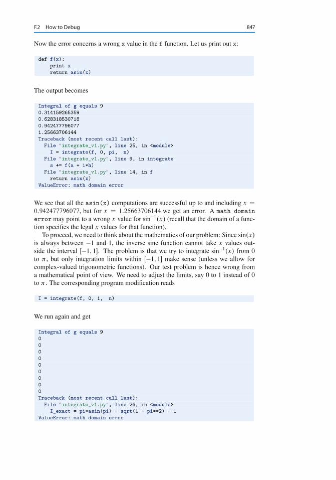
F.2 How to Debug 847
Now the error concerns a wrong x value in the f function. Let us print out x:
def f(x):
print x
return asin(x)
The output becomes
Integral of g equals 9
0.314159265359
0.628318530718
0.942477796077
1.25663706144
Traceback (most recent call last):
File "integrate_v1.py", line 25, in <module>
I = integrate(f, 0, pi, n)
File "integrate_v1.py", line 9, in integrate
s += f(a + i*h)
File "integrate_v1.py", line 14, in f
return asin(x)
ValueError: math domain error
We see that all the asin(x) computations are successful up to and including x D0:942477796077, but for x D 1:25663706144 we get an error. A math domainerrormay point to a wrong x value for sin�1.x/ (recall that the domain of a func-tion specifies the legal x values for that function).
To proceed, we need to think about the mathematics of our problem: Since sin.x/
is always between �1 and 1, the inverse sine function cannot take x values out-side the interval Œ�1; 1�. The problem is that we try to integrate sin�1.x/ from 0to � , but only integration limits within Œ�1; 1� make sense (unless we allow forcomplex-valued trigonometric functions). Our test problem is hence wrong froma mathematical point of view. We need to adjust the limits, say 0 to 1 instead of 0to � . The corresponding program modification reads
I = integrate(f, 0, 1, n)
We run again and get
Integral of g equals 9
0
0
0
0
0
0
0
0
0
Traceback (most recent call last):
File "integrate_v1.py", line 26, in <module>
I_exact = pi*asin(pi) - sqrt(1 - pi**2) - 1
ValueError: math domain error
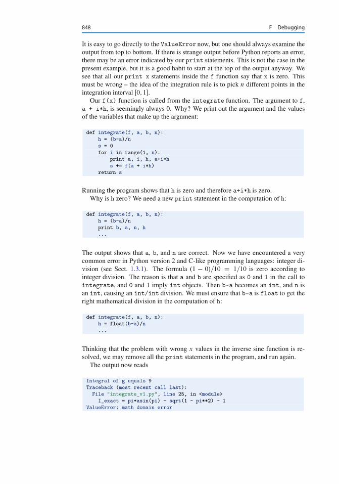
848 F Debugging
It is easy to go directly to the ValueError now, but one should always examine theoutput from top to bottom. If there is strange output before Python reports an error,there may be an error indicated by our print statements. This is not the case in thepresent example, but it is a good habit to start at the top of the output anyway. Wesee that all our print x statements inside the f function say that x is zero. Thismust be wrong – the idea of the integration rule is to pick n different points in theintegration interval Œ0; 1�.
Our f(x) function is called from the integrate function. The argument to f,a + i*h, is seemingly always 0. Why? We print out the argument and the valuesof the variables that make up the argument:
def integrate(f, a, b, n):
h = (b-a)/n
s = 0
for i in range(1, n):
print a, i, h, a+i*h
s += f(a + i*h)
return s
Running the program shows that h is zero and therefore a+i*h is zero.Why is h zero? We need a new print statement in the computation of h:
def integrate(f, a, b, n):
h = (b-a)/n
print b, a, n, h
...
The output shows that a, b, and n are correct. Now we have encountered a verycommon error in Python version 2 and C-like programming languages: integer di-vision (see Sect. 1.3.1). The formula .1 � 0/=10 D 1=10 is zero according tointeger division. The reason is that a and b are specified as 0 and 1 in the call tointegrate, and 0 and 1 imply int objects. Then b-a becomes an int, and n isan int, causing an int/int division. We must ensure that b-a is float to get theright mathematical division in the computation of h:
def integrate(f, a, b, n):
h = float(b-a)/n
...
Thinking that the problem with wrong x values in the inverse sine function is re-solved, we may remove all the print statements in the program, and run again.
The output now reads
Integral of g equals 9
Traceback (most recent call last):
File "integrate_v1.py", line 25, in <module>
I_exact = pi*asin(pi) - sqrt(1 - pi**2) - 1
ValueError: math domain error
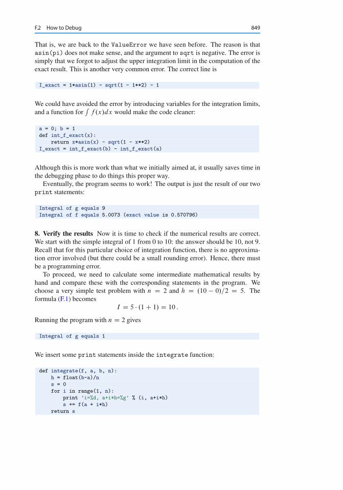
F.2 How to Debug 849
That is, we are back to the ValueError we have seen before. The reason is thatasin(pi) does not make sense, and the argument to sqrt is negative. The error issimply that we forgot to adjust the upper integration limit in the computation of theexact result. This is another very common error. The correct line is
I_exact = 1*asin(1) - sqrt(1 - 1**2) - 1
We could have avoided the error by introducing variables for the integration limits,and a function for
Rf .x/dx would make the code cleaner:
a = 0; b = 1
def int_f_exact(x):
return x*asin(x) - sqrt(1 - x**2)
I_exact = int_f_exact(b) - int_f_exact(a)
Although this is more work than what we initially aimed at, it usually saves time inthe debugging phase to do things this proper way.
Eventually, the program seems to work! The output is just the result of our twoprint statements:
Integral of g equals 9
Integral of f equals 5.0073 (exact value is 0.570796)
8. Verify the results Now it is time to check if the numerical results are correct.We start with the simple integral of 1 from 0 to 10: the answer should be 10, not 9.Recall that for this particular choice of integration function, there is no approxima-tion error involved (but there could be a small rounding error). Hence, there mustbe a programming error.
To proceed, we need to calculate some intermediate mathematical results byhand and compare these with the corresponding statements in the program. Wechoose a very simple test problem with n D 2 and h D .10 � 0/=2 D 5. Theformula (F.1) becomes
I D 5 � .1 C 1/ D 10 :
Running the program with n D 2 gives
Integral of g equals 1
We insert some print statements inside the integrate function:
def integrate(f, a, b, n):
h = float(b-a)/n
s = 0
for i in range(1, n):
print ’i=%d, a+i*h=%g’ % (i, a+i*h)
s += f(a + i*h)
return s
850 F Debugging
Here is the output:
i=1, a+i*h=5
Integral of g equals 1
i=1, a+i*h=0.5
Integral of f equals 0.523599 (exact value is 0.570796)
There was only one pass in the i loop in integrate. According to the formula,there should be n passes, i.e., two in this test case. The limits of i must be wrong.The limits are produced by the call range(1,n). We recall that such a call resultsin integers going from 1 up to n, but not including n. We need to include n as valueof i, so the right call to range is range(1,n+1).
We make this correction and rerun the program. The output is now
i=1, a+i*h=5
i=2, a+i*h=10
Integral of g equals 2
i=1, a+i*h=0.5
i=2, a+i*h=1
Integral of f equals 2.0944 (exact value is 0.570796)
The integral of 1 is still not correct. We need more intermediate results!In our quick hand calculation we knew that g.x/ D 1 so all the f .a C .i � 1
2/h/
evaluations were rapidly replaced by ones. Let us now compute all the x coordinatesa C .i � 1
2/h that are used in the formula:
i D 1 W a C�
i � 1
2
�h D 2:5; i D 2 W a C
�i � 1
2
�h D 7:5 :
Looking at the output from the program, we see that the argument to g has a differ-ent value – and fortunately we realize that the formula we have coded is wrong. Itshould be a+(i-0.5)*h.
We correct this error and run the program:
i=1, a+(i-0.5)*h=2.5
i=2, a+(i-0.5)*h=7.5
Integral of g equals 2
...
Still the integral is wrong. At this point youmay give up programming, but the moreskills you pick up in debugging, the more fun it is to hunt for errors! Debuggingis like reading an exciting criminal novel: the detective follows different ideas andtracks, but never gives up before the culprit is caught.
Now we read the code more carefully and compare expressions with those in themathematical formula. We should, of course, have done this already when writingthe program, but it is easy to get excited when writing code and hurry for the end.This ongoing story of debugging probably shows that reading the code carefullycan save much debugging time. (Actually, being extremely careful with what youwrite, and comparing all formulas with the mathematics, may be the best way to getmore spare time when taking a programming course!)
F.2 How to Debug 851
We clearly add up all the f evaluations correctly, but then this sum must be mul-tiplied by h, and we forgot that in the code. The return statement in integratemust therefore be modified to
return s*h
Eventually, the output is
Integral of g equals 10
Integral of f equals 0.568484 (exact value is 0.570796)
and we have managed to integrate a constant function in our program! Even thesecond integral looks promising!
To judge the result of integrating the inverse sine function, we need to runseveral increasing n values and see that the approximation gets better. For n D2; 10; 100; 1000 we get 0.550371, 0.568484, 0.570714, 0.570794, to be comparedto the exact value 0.570796. (This is not the mathematically exact value, because itinvolves computations of sin�1.x/, which is only approximately calculated by theasin function in the mathmodule. However, the approximation error is very small(� 10�16).) The decreasing error provides evidence for a correct program, but it isnot a strong proof. We should try out more functions. In particular, linear functionsare integrated exactly by the Midpoint rule. We can also measure the speed of thedecrease of the error and check that the speed is consistent with the properties ofthe Midpoint rule, but this is a mathematically more advanced topic.
The very important lesson learned from these debugging sessions is that youshould start with a simple test problem where all formulas can be computed byhand. If you start out with n D 100 and try to integrate the inverse sine function,you will have a much harder job with tracking down all the errors.
9. Use a debugger Another lesson learned from these sessions is that we neededmany print statements to see intermediate results. It is an open question if itwould be more efficient to run a debugger and stop the code at relevant lines. In anedit-and-run cycle of the type we met here, we frequently need to examine manynumerical results, correct something, and look at all the intermediate results again.Plain print statements are often better suited for this massive output than the puremanual operation of a debugger, unless one writes a program to automate the inter-action with the debugger.
The correct code for the implementation of the Midpoint rule is found inintegrate_v2.py. Some readers might be frightened by all the energy it tookto debug this code, but this is just the nature of programming. The experience ofdeveloping programs that finally work is very awarding.
People only become computer programmers if they’re obsessive about details, crave powerover machines, and can bear to be told day after day exactly how stupid they are. GregoryJ. E. Rawlins [24], computer scientist.
Refining the user interface We briefly mentioned that the chosen user interface,where the user can only specify n, is not particularly user friendly. We should
852 F Debugging
allow f , a, b, and n to be specified on the command line. Since f is a functionand the command line can only provide strings to the program, we may use theStringFunction object from scitools.std to convert a string expression forthe function to be integrated to an ordinary Python function (see Sect. 4.3.3). Theother parameters should be easy to retrieve from the command line if Sect. 4.2is understood. As suggested in Sect. 4.7, we enclose the input statements ina try-except block, here with a specific exception type IndexError (because anindex in sys.argv out of bounds is the only type of error we expect to handle):
try:
f_formula = sys.argv[1]
a = eval(sys.argv[2])
b = eval(sys.argv[3])
n = int(sys.argv[4])
except IndexError:
print ’Usage: %s f-formula a b n’ % sys.argv[0]
sys.exit(1)
Note that the use of eval allows us to specify a and b as pi or exp(5) or anothermathematical expression.
With the input above we can perform the general task of the program:
from scitools.std import StringFunction
f = StringFunction(f_formula)
I = integrate(f, a, b, n)
print I
Writing a test function Instead of having these test statements as a main programwe follow the good habits of Sect. 4.9 and make a module with
the integrate function, a test_integrate function for testing the integrate function’s ability to ex-
actly integrate linear functions, a main function for reading data from the command line and calling integrate
for the user’s problem at hand.
Any module should also have a test block, as well as doc strings for the moduleitself and all functions.
The test_integrate function can perform a loop over some specified n valuesand check that the Midpoint rule integrates a linear function exactly. As always,we must be prepared for rounding errors, so “exactly” means errors less than (say)10�14. The relevant code becomes
def test_integrate():
"""Check that linear functions are integrated exactly."""
def g(x):
return p*x + q # general linear function
def int_g_exact(x): # integral of g(x)
return 0.5*p*x**2 + q*x
F.2 How to Debug 853
a = -1.2; b = 2.8 # "arbitrary" integration limits
p = -2; q = 10
success = True # True if all tests below are passed
for n in 1, 10, 100:
I = integrate(g, a, b, n)
I_exact = int_g_exact(b) - int_g_exact(a)
error = abs(I_exact - I)
if error > 1E-14:
success = False
assert success
We have followed the programming standard that will make this test function auto-matically work with the nose test framework:
1. the name of the function starts with test_,2. the function has no arguments,3. checks of whether a test is passed or not are done with assert.
The assert success statement raises an AssertionError exception if successis false, otherwise nothing happens. The nose testing framework searches forfunctions whose name start with test_, execute each function, and record if anAssertionError is raised. It is overkill to use nose for small programs, but inlarger projects with many functions in many files, nose can run all tests with a shortcommand and write back a notification that all tests passed.
The main function is simply a wrapping of the main program given above. Thetest block may call or test_integrate function or main, depending on whetherthe user will test the module or use it:
if __name__ == ’__main__’:
if sys.argv[1] == ’verify’:
verify()
else:
# Compute the integral specified on the command line
main()
Here is a short demo computingR 2�
0.cos.x/ C sin.x//dx with the aid of the
integrate.py file:
Terminal
integrate.py ’cos(x)+sin(x)’ 0 2*pi 10-3.48786849801e-16
F.2.3 Getting Help from a Code Analyzer
The tools PyLint3 and Flake84 can analyze your code and point out errors and un-desired coding styles. Before point 7 in the lists above, Run the program, it can
3 http://www.pylint.org/4 https://flake8.readthedocs.org/en/2.0/
854 F Debugging
be wise to run PyLint and/or Flake8 to be informed about problems with the code.Flake8 complains in general a lot less than PyLint, and might be a more useful toolfor mathematical software (see the examples below), but both tools are very usefulduring program development to improve your code and ease further debugging.
Consider the first version of the integrate code, integrate_v1.py. RunningFlake8 gives
Terminal
Terminal> flake8 integrate_v1.pyintegrate_v1.py:7:1: E302 expected 2 blank lines, found 1integrate_v1.py:8:1: E112 expected an indented blockintegrate_v1.py:8:7: E901 IndentationError: expected an indented blockintegrate_v1.py:10:1: E302 expected 2 blank lines, found 1integrate_v1.py:11:1: E112 expected an indented block
Flake8 checks if the program obeys the official Style Guide for Python Code5
(known as PEP8). One of the rules in this guide is to have two blank lines beforefunctions and classes (a habit that is often dropped in this book to reduce the lengthof code snippets), and our program breaks the rule before the f and g functions.More serious and useful is the notification of expected an indented block atlines 8 and 11, but this error is quickly found by running the program too.
PyLint reports much less about integrate_v1.py:
Terminal
Terminal> pylint integrate_v1.pyE: 8, 0: expected an indented block (syntax-error)
Running Flak8 on integrate_v2.py leads to only three problems: missing twoblank lines before functions and doing from math import *. Applying PyLint tointegrate_v2.py results in many more problems:
Terminal
Terminal> pylint integrate_v2.pyC: 20, 0: Exactly one space required after commaI = integrate(f, 0, 1, n)
^ (bad-whitespace)W: 19, 0: Redefining built-in ’pow’ (redefined-builtin)C: 1, 0: Missing module docstring (missing-docstring)W: 1,14: Redefining name ’f’ from outer scope (line 8)W: 1,23: Redefining name ’n’ from outer scope (line 16)C: 1, 0: Invalid argument name "f" (invalid-name)C: 1, 0: Invalid argument name "a" (invalid-name)
There is much more output, but let us summarize what PyLint does not like aboutthe code:
1. Extra whitespace (after comma in a call to integrate)2. Missing doc string at the beginning of the file
5 http://www.python.org/dev/peps/pep-0008/

F.2 How to Debug 855
3. Missing doc strings in the functions4. Same name f used as local variable in integrate and global function name in
the f(x) function5. Too short variable names: a, b, n, etc.6. “Star import” of the form from math import *
In short programs where the one-to-one mapping between mathematical notationand the variable names is very important to make the code self-explanatory, thisauthor thinks that only points 1–3 qualify for attention. Nevertheless, for largernon-mathematical programs all the style violations pointed out are serious and leadto code that is easier to read, debug, maintain, and use.
GMigrating Python to Compiled Code
Python is a very convenient language for implementing scientific computations asthe code can be made very close to the mathematical algorithms. However, theexecution speed of the code is significantly lower than what can be obtained byprogramming in languages such as Fortran, C, or C++. These languages compile theprogram to machine language, which enables the computing resources to be utilizedwith very high efficiency. Frequently, and this includes almost all examples in thepresent book, Python is fast enough. But in the cases where speed really matters,can we increase the efficiency without rewriting the whole program in Fortran, C,or C++? The answer is yes, which will be illustrated through a case study in theforthcoming text.
Fortunately, Python was initially designed for being integrated with C. Thisfeature has spawned the development of several techniques and tools for callingcompiled languages from Python, allowing us to relatively easily reuse fast andwell-tested scientific libraries in Fortran, C, or C++ from Python, or migrate slowPython code to compiled languages. It often turns out that only smaller parts ofthe code, usually for loops doing heavy numerical computations, suffer from lowspeed and can benefit from being implemented in Fortran, C, or C++.
The primary technique to be advocated here is to use Cython. Cython can beviewed as an extension of the Python language where variables can be declaredwith a type and other information such that Cython is able to automatically generatespecial-purpose, fast C code from the Python code. We will show how to utilizeCython and what the computational gain might be.
The present case study starts with stating a computational problem involvingstatistical simulations, which are known to cause long execution times, especially ifaccurate results are desired.
G.1 Pure Python Code for Monte Carlo Simulation
A short, intuitive algorithm in Python is first developed. Then this code is vectorizedusing functionality of the Numerical Python package. Later sections migrate thealgorithm to Cython code and also plain C code for comparison. At the end thevarious techniques are ranked according to their computational efficiency.
857
858 G Migrating Python to Compiled Code
G.1.1 The Computational Problem
A die is thrown m times. What is the probability of getting six eyes at least n times?For example, if m D 5 and n D 3, this is the same as asking for the probability thatthree or more out of five dice show six eyes.
The probability can be estimated by Monte Carlo simulation. Chapter 8.3 pro-vides a background for this technique: We simulate the process a large number oftimes, N , and count how many times, M , the experiment turned out successfully,i.e., when we got at least n out of m dice with six eyes in a throw.
Monte Carlo simulation has traditionally been viewed as a very costly compu-tational method, normally requiring very sophisticated, fast computer implemen-tations in compiled languages. An interesting question is how useful high-levellanguages like Python and associated tools are for Monte Carlo simulation. Thiswill now be explored.
G.1.2 A Scalar Python Implementation
Let us introduce the more descriptive variables ndice for m and nsix for n. TheMonte Carlo method is simply a loop, repeated N times, where the body of the loopmay directly express the problem at hand. Here, we draw ndice random integers rin Œ1; 6� inside the loop and count of many (six) that equal 6. If six >= nsix, theexperiment is a success and we increase the counter M by one.
A Python function implementing this approach may look as follows:
import random
def dice6_py(N, ndice, nsix):
M = 0 # no of successful events
for i in range(N): # repeat N experiments
six = 0 # how many dice with six eyes?
for j in range(ndice):
r = random.randint(1, 6) # roll die no. j
if r == 6:
six += 1
if six >= nsix: # successful event?
M += 1
p = float(M)/N
return p
The float(M) transformation is important since M/N will imply integer divisionwhen M and N both are integers in Python v2.x and many other languages.
We will refer to this implementation is the plain Python implementation. Timingthe function can be done by:
import time
t0 = time.clock()
p = dice6_py(N, ndice, nsix)
t1 = time.clock()
print ’CPU time for loops in Python:’, t1-t0
G.1 Pure Python Code for Monte Carlo Simulation 859
The table to appear later shows the performance of this plain, pure Python coderelative to other approaches. There is a factor of 30+ to be gained in computationalefficiency by reading on.
The function above can be verified by studying the (somewhat simplified) casem D n where the probability becomes 6�n. The probability quickly becomes smallwith increasing n. For such small probabilities the number of successful eventsM is small, and M=N will not be a good approximation to the probability unlessM is reasonably large, which requires a very large N . For example, with n D 4
and N D 105 the average probability in 25 full Monte Carlo experiments is 0.00078while the exact answer is 0.00077. With N D 106 we get the two correct significantdigits from the Monte Carlo simulation, but the extra digit costs a factor of 10 incomputing resources since the CPU time scales linearly with N .
G.1.3 A Vectorized Python Implementation
A vectorized version of the previous program consists of replacing the explicit loopsin Python by efficient operations on vectors or arrays, using functionality in the Nu-merical Python (numpy) package. Each array operation takes place in C or Fortranand is hence much more efficient than the corresponding loop version in Python.
First, we must generate all the random numbers to be used in one operation,which runs fast since all numbers are then calculated in efficient C code. This isaccomplished using the numpy.randommodule. Second, the analysis of the largecollection of random numbers must be done by appropriate vector/array operationssuch that no looping in Python is needed. The solution algorithm must thereforebe expressed through a series of function calls to the numpy library. Vectorizationrequires knowledge of the library’s functionality and how to assemble the relevantbuilding blocks to an algorithm without operations on individual array elements.
Generation of ndice random number of eyes for N experiments is performed by
import numpy as np
eyes = np.random.random_integers(1, 6, size=(N, ndice))
Each row in the eyes array corresponds to one Monte Carlo experiment.The next step is to count the number of successes in each experiment. This
counting should not make use of any loop. Instead we can test eyes == 6 to geta boolean array where an element i,j is True if throw (or die) number j in MonteCarlo experiment number i gave six eyes. Summing up the rows in this booleanarray (True is interpreted as 1 and False as 0), we are interested in the rows wherethe sum is equal to or greater than nsix, because the number of such rows equalsthe number of successful events. The vectorized algorithm can be expressed as
def dice6_vec1(N, ndice, nsix):
eyes = np.random.random_integers(1, 6, size=(N, ndice))
compare = eyes == 6
throws_with_6 = np.sum(compare, axis=1) # sum over columns
nsuccesses = throws_with_6 >= nsix
M = np.sum(nsuccesses)
p = float(M)/N
return p
860 G Migrating Python to Compiled Code
The use of np.sum instead of Python’s own sum function is essential for thespeed of this function: using M = sum(nsucccesses) instead slows down thecode by a factor of almost 10! We shall refer to the dice6_vec1 function as thevectorized Python, version1 implementation.
The criticism against the vectorized version is that the original problem descrip-tion, which was almost literally turned into Python code in the dice6_py function,has now become much more complicated. We have to decode the calls to variousnumpy functionality to actually realize that dice6_py and dice6_vec correspondto the same mathematics.
Here is another possible vectorized algorithm, which is easier to understand,because we retain the Monte Carlo loop and vectorize only each individual experi-ment:
def dice6_vec2(N, ndice, nsix):
eyes = np.random.random_integers(1, 6, (N, ndice))
six = [6 for i in range(ndice)]
M = 0
for i in range(N):
# Check experiment no. i:
compare = eyes[i,:] == six
if np.sum(compare) >= nsix:
M += 1
p = float(M)/N
return p
We refer to this implementation as vectorized Python, version 2. As will beshown later, this implementation is significantly slower than the plain Python im-plementation (!) and very much slower than the vectorized Python, version 1approach. A conclusion is that readable, partially vectorized code, may run slowerthan straightforward scalar code.
G.2 Migrating Scalar Python Code to Cython
G.2.1 A Plain Cython Implementation
A Cython program starts with the scalar Python implementation, but all variablesare specified with their types, using Cython’s variable declaration syntax, like cdefint M = 0 where we in standard Python just write M = 0. Adding such variabledeclarations in the scalar Python implementation is straightforward:
import random
def dice6_cy1(int N, int ndice, int nsix):
cdef int M = 0 # no of successful events
cdef int six, r
cdef double p
for i in range(N): # repeat N experiments
six = 0 # how many dice with six eyes?
for j in range(ndice):
r = random.randint(1, 6) # roll die no. j
G.2 Migrating Scalar Python Code to Cython 861
if r == 6:
six += 1
if six >= nsix: # successful event?
M += 1
p = float(M)/N
return p
This code must be put in a separate file with extension .pyx. Running Cython onthis file translates the Cython code to C. Thereafter, the C code must be compiledand linked to form a shared library, which can be imported in Python as a module.All these tasks are normally automated by a setup.py script. Let the dice6_cy1function above be stored in a file dice6.pyx. A proper setup.py script looks asfollows:
from distutils.core import setup
from distutils.extension import Extension
from Cython.Distutils import build_ext
setup(
name=’Monte Carlo simulation’,
ext_modules=[Extension(’_dice6_cy’, [’dice6.pyx’],)],
cmdclass={’build_ext’: build_ext},
)
Running
Terminal
Terminal> python setup.py build_ext --inplace
generates the C code and creates a (shared library) file _dice6_cy.so (known asa C extension module) which can be loaded into Python as a module with name_dice6_cy:
from _dice6_cy import dice6_cy1
import time
t0 = time.clock()
p = dice6_cy1(N, ndice, nsix)
t1 = time.clock()
print t1 - t0
We refer to this implementation as Cython random.randint. Although most of thestatements in the dice6_cy1 function are turned into plain and fast C code, thespeed is not much improved compared with the original scalar Python code.
To investigate what takes time in this Cython implementation, we can performa profiling. The template for profiling a Python function whose call syntax is storedin some string statement, reads
import cProfile, pstats
cProfile.runctx(statement, globals(), locals(), ’tmp_profile.dat’)
s = pstats.Stats(’tmp_profile.dat’)
s.strip_dirs().sort_stats(’time’).print_stats(30)
862 G Migrating Python to Compiled Code
Data from the profiling are here stored in the file tmp_profile.dat. Our interestnow is the dice6_cy1 function so we set
statement = ’dice6_cy1(N, ndice, nsix)’
In addition, a Cython file in which there are functions we want to profile must startwith the line
# cython: profile=True
to turn on profiling when creating the extension module. The profiling output fromthe present example looks like
5400004 function calls in 7.525 CPU seconds
Ordered by: internal time
ncalls tottime percall cumtime percall filename:lineno(function)
1800000 4.511 0.000 4.863 0.000 random.py:160(randrange)
1800000 1.525 0.000 6.388 0.000 random.py:224(randint)
1 1.137 1.137 7.525 7.525 dice6.pyx:6(dice6_cy1)
1800000 0.352 0.000 0.352 0.000 {method ’random’ ...
1 0.000 0.000 7.525 7.525 {dice6_cy.dice6_cy1}
We easily see that it is the call to random.randint that consumes almost all thetime. The reason is that the generated C code must call a Python module (random),which implies a lot of overhead. The C code should only call plain C functions, orif Python functions must be called, they should involve so much computations thatthe overhead in calling Python from C is negligible.
Instead of profiling the code to uncover inefficient constructs we can generatea visual representation of how the Python code is translated to C. Running
Terminal
Terminal> cython -a dice6.pyx
creates a file dice6.html which can be loaded into a web browser to inspect whatCython has done with the Python code.
G.2 Migrating Scalar Python Code to Cython 863
White lines indicate that the Python code is translated into C code, while theyellow lines indicate that the generated C code must make calls back to Python(using the Python C API, which implies overhead). Here, the random.randintcall is in yellow, so this call is not translated to efficient C code.
G.2.2 A Better Cython Implementation
To speed up the previous Cython code, we have to get rid of the random.randintcall every time we need a random variable. Either we must call some C functionfor generating a random variable or we must create a bunch of random numberssimultaneously as we did in the vectorized functions shown above. We first try thelatter well-known strategy and apply the numpy.randommodule to generate all therandom numbers we need at once:
import numpy as np
cimport numpy as np
@cython.boundscheck(False) # turn off array bounds check
@cython.wraparound(False) # turn off negative indices ([-1,-1])
def dice6_cy2(int N, int ndice, int nsix):
# Use numpy to generate all random numbers
...
cdef np.ndarray[np.int_t, ndim=2, mode=’c’] eyes = \
np.random.random_integers(1, 6, (N, ndice))
This code needs some explanation. The cimport statement imports a special ver-sion of numpy for Cython and is needed after the standard numpy import. Thedeclaration of the array of random numbers could just go as
cdef np.ndarray eyes = np.random.random_integers(1, 6, (N, ndice))
However, the processing of the eyes array will then be slow because Cython doesnot have enough information about the array. To generate optimal C code, we mustprovide information on the element types in the array, the number of dimensionsof the array, that the array is stored in contiguous memory, that we do not wantthe overhead of checking whether indices are within their bounds or not, and thatwe do not need negative indices (which slows down array indexing). The lattertwo properties are taken care of by the @cython.boundscheck(False) and [email protected](False) statements (decorators) right before the function,respectively, while the rest of the information is specified within square brackets inthe cdef np.ndarray declaration. Inside the brackets, np.int_t denotes integerarray elements (np.int is the usual data type object, but np.int_t is a Cythonprecompiled version of this object), ndim=2 tells that the array has two dimensions(indices), and mode=’c’ indicates contiguous storage of the array. With all thisextra information, Cython can generate C code that works with numpy arrays asefficiently as native C arrays.
The rest of the code is a plain copy of the dice6_py function, but with therandom.randint call replaced by an array look-up eyes[i,j] to retrieve the next
864 G Migrating Python to Compiled Code
random number. The two loops will now be as efficient as if they were codeddirectly in pure C.
The complete code for the efficient version of the dice6_cy1 function looks asfollows:
import numpy as np
cimport numpy as np
import cython
@cython.boundscheck(False) # turn off array bounds check
@cython.wraparound(False) # turn off negative indices ([-1,-1])
def dice6_cy2(int N, int ndice, int nsix):
# Use numpy to generate all random numbers
cdef int M = 0 # no of successful events
cdef int six, r
cdef double p
cdef np.ndarray[np.int_t, ndim=2, mode=’c’] eyes = \
np.random.random_integers(1, 6, (N, ndice))
for i in range(N):
six = 0 # how many dice with six eyes?
for j in range(ndice):
r = eyes[i,j] # roll die no. j
if r == 6:
six += 1
if six >= nsix: # successful event?
M += 1
p = float(M)/N
return p
This Cython implementation is named Cython numpy.random.The disadvantage with the dice6_cy2 function is that large simulations (large
N) also require large amounts of memory, which usually limits the possibility forhigh accuracy much more than the CPU time. It would be advantageous to havea fast random number generator a la random.randint in C. The C library stdlibhas a generator of random integers, rand(), generating numbers from 0 to upRAND_MAX. Both the rand function and the RAND_MAX integer are easy to accessin a Cython program:
from libc.stdlib cimport rand, RAND_MAX
r = 1 + int(6.0*rand()/RAND_MAX) # random integer 1,...,6
Note that rand() returns an integer so we must avoid integer division by ensur-ing that the denominator is a real number. We also need to explicitly convert theresulting real fraction to int since r is declared as int.
With this way of generating random numbers we can create a version ofdice6_cy1 that is as fast as dice6_cy, but avoids all the memory demandsand the somewhat complicated array declarations of the latter:
from libc.stdlib cimport rand, RAND_MAX
def dice6_cy3(int N, int ndice, int nsix):
cdef int M = 0 # no of successful events
cdef int six, r
G.3 Migrating Code to C 865
cdef double p
for i in range(N):
six = 0 # how many dice with six eyes?
for j in range(ndice):
# Roll die no. j
r = 1 + int(6.0*rand()/RAND_MAX)
if r == 6:
six += 1
if six >= nsix: # successful event?
M += 1
p = float(M)/N
return p
This final Cython implementation will be referred to as Cython stdlib.rand.
G.3 Migrating Code to C
G.3.1 Writing a C Program
A natural next improvement would be to program the Monte Carlo simulation loopsdirectly in a compiled programming language, which guarantees optimal speed.Here we choose the C programming language for this purpose. The C version ofour dice6 function and an associated main program take the form
#include <stdio.h>
#include <stdlib.h>
double dice6(int N, int ndice, int nsix)
{
int M = 0;
int six, r, i, j;
double p;
for (i = 0; i < N; i++) {
six = 0;
for (j = 0; j < ndice; j++) {
r = 1 + rand()/(RAND_MAX*6.0); /* roll die no. j */
if (r == 6)
six += 1;
}
if (six >= nsix)
M += 1;
}
p = ((double) M)/N;
return p;
}
int main(int nargs, const char* argv[])
{
int N = atoi(argv[1]);
int ndice = 6;
int nsix = 3;
866 G Migrating Python to Compiled Code
double p = dice6(N, ndice, nsix);
printf("C code: N=%d, p=%.6f\n", N, p);
return 0;
}
This code is placed in a file dice6_c.c. The file can typically be compiled andrun by
Terminal
Terminal> gcc -O3 -o dice6.capp dice6_c.cTerminal> ./dice6.capp 1000000
This solution is later referred to as C program.
G.3.2 Migrating Loops to C Code via F2PY
Instead of programming the whole application in C, we may consider migrating theloops to the C function dice6 shown above and then have the rest of the program(essentially the calling main program) in Python. This is a convenient solution ifwe were to do many other, less CPU time critical things for convenience in Python.
There are many alternative techniques for calling C functions from Python. Herewe shall explain two. The first applies the program f2py to generate the necessarycode that glues Python and C. The f2py program was actually made for gluingPython and Fortran, but it can work with C too. We need a specification of theC function to call in terms of a Fortran 90 module. Such a module can be writ-ten by hand, but f2py can also generate it. To this end, we make a Fortran filedice6_c_signature.fwith the signature of the C function written in Fortran 77syntax with some annotations:
real*8 function dice6(n, ndice, nsix)
Cf2py intent(c) dice6
integer n, ndice, nsix
Cf2py intent(c) n, ndice, nsix
return
end
The annotations intent(c) are necessary to tell f2py that the Fortran variablesare to be treated as plain C variables and not as pointers (which is the default inter-pretation of variables in Fortran). The C2fpy are special comment lines that f2pyrecognizes, and these lines are used to provide extra information to f2py whichhave no meaning in plain Fortran 77.
We must run f2py to generate a .pyf file with a Fortran 90 module specificationof the C function to call:
Terminal
Terminal> f2py -m _dice6_c1 -h dice6_c.pyf \dice6_c_signature.f
G.3 Migrating Code to C 867
Here _dice6_c1 is the name of the module with the C function that is to be im-ported in Python, and dice6_c.pyf is the name of the Fortran 90 module file to begenerated. Programmers who know Fortran 90 may want to write the dice6_c.pyffile by hand.
The next step is to use the information in dice6_c.pyf to generate a (C ex-tension) module _dice6_c1. Fortunately, f2py generates the necessary code, andcompiles and links the relevant files, to form a shared library file _dice6_c1.so,by a short command:
Terminal
Terminal> f2py -c dice6_c.pyf dice6_c.c
We can now test the module:
>>> import _dice6_c1
>>> print dir(_dice6_c1) # module contents
[’__doc__’, ’__file__’, ’__name__’, ’__package__’,
’__version__’, ’dice6’]
>>> print _dice6_c1.dice6.__doc__
dice6 - Function signature:
dice6 = dice6(n,ndice,nsix)
Required arguments:
n : input int
ndice : input int
nsix : input int
Return objects:
dice6 : float
>>> _dice6_c1.dice6(N=1000, ndice=4, nsix=2)
0.145
The method of calling the C function dice6 via an f2py generated module is re-ferred to as C via f2py.
G.3.3 Migrating Loops to C Code via Cython
The Cython tool can also be used to call C code, not only generating C code fromthe Cython language. Our C code is in the file dice6_c.c, but for Cython to seethis code we need to create a header file dice6_c.h listing the definition of thefunction(s) we want to call from Python. The header file takes the form
extern double dice6(int N, int ndice, int nsix);
The next step is to make a .pyx file with a definition of the C function from theheader file and a Python function that calls the C function:
cdef extern from "dice6_c.h":
double dice6(int N, int ndice, int nsix)
def dice6_cwrap(int N, int ndice, int nsix):
return dice6(N, ndice, nsix)
868 G Migrating Python to Compiled Code
Cython must use this file, named dice6_cwrap.pyx, to generate C code, whichis to be compiled and linked with the dice6_c.c code. All this is accomplished ina setup.py script:
from distutils.core import setup
from distutils.extension import Extension
from Cython.Distutils import build_ext
sources = [’dice6_cwrap.pyx’, ’dice6_c.c’]
setup(
name=’Monte Carlo simulation’,
ext_modules=[Extension(’_dice6_c2’, sources)],
cmdclass={’build_ext’: build_ext},
)
This setup.py script is run as
Terminal
Terminal> python setup.py build_ext --inplace
resulting in a shared library file _dice6_c2.so, which can be loaded into Pythonas a module:
>>> import _dice6_c2
>>> print dir(_dice6_c2)
[’__builtins__’, ’__doc__’, ’__file__’, ’__name__’,
’__package__’, ’__test__’, ’dice6_cwrap’]
We see that the module contains the function dice6_cwrap, which was made tocall the underlying C function dice6.
G.3.4 Comparing Efficiency
All the files corresponding to the various techniques described above are avail-able in the directory src/cython. A file make.sh performs all the compilations,while compare.py runs all methods and prints out the CPU time required by eachmethod, normalized by the fastest approach. The results for N D 450; 000 arelisted below (MacBook Air running Ubuntu in a VMWare Fusion virtual machine).
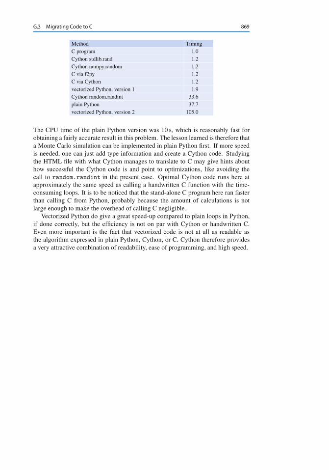
G.3 Migrating Code to C 869
Method TimingC program 1.0Cython stdlib.rand 1.2Cython numpy.random 1.2C via f2py 1.2C via Cython 1.2vectorized Python, version 1 1.9Cython random.randint 33.6plain Python 37.7vectorized Python, version 2 105.0
The CPU time of the plain Python version was 10 s, which is reasonably fast forobtaining a fairly accurate result in this problem. The lesson learned is therefore thata Monte Carlo simulation can be implemented in plain Python first. If more speedis needed, one can just add type information and create a Cython code. Studyingthe HTML file with what Cython manages to translate to C may give hints abouthow successful the Cython code is and point to optimizations, like avoiding thecall to random.randint in the present case. Optimal Cython code runs here atapproximately the same speed as calling a handwritten C function with the time-consuming loops. It is to be noticed that the stand-alone C program here ran fasterthan calling C from Python, probably because the amount of calculations is notlarge enough to make the overhead of calling C negligible.
Vectorized Python do give a great speed-up compared to plain loops in Python,if done correctly, but the efficiency is not on par with Cython or handwritten C.Even more important is the fact that vectorized code is not at all as readable asthe algorithm expressed in plain Python, Cython, or C. Cython therefore providesa very attractive combination of readability, ease of programming, and high speed.
HTechnical Topics
H.1 Getting Access to Python
A comprehensive eco system for scientific computing with Python used to be quitea challenge to install on a computer, especially for newcomers. This problem ismore or less solved today. There are several options for getting easy access toPython and the most important packages for scientific computations, so the biggestissue for a newcomer is to make a proper choice. An overview of the possibilitiestogether with my own recommendations appears next.
H.1.1 Required Software
The strictly required software packages for working with this book are
Python1 version 2.7 [23] Numerical Python2 (NumPy) [19, 20] for array computing Matplotlib3 [8, 9] for plotting
Desired add-on packages are
IPython4 [21, 22] for interactive computing SciTools5 [14] for add-ons to NumPy pytest6 or nose7 for testing programs pip8 for installing Python packages Cython9 for compiling Python to C
1 http://python.org2 http://www.numpy.org3 http://matplotlib.org4 http://ipython.org5 https://github.com/hplgit/scitools6 http://pytest.org/latest/7 https://nose.readthedocs.org8 http://www.pip-installer.org9 http://cython.org
871
872 H Technical Topics
SymPy10 [2] for symbolic mathematics SciPy11 [10] for advanced scientific computing
There are different ways to get access to Python with the required packages:
1. Use a computer system at an institution where the software is installed. Sucha system can also be used from your local laptop through remote login overa network.
2. Install the software on your own laptop.3. Use a web service.
A system administrator can take the list of software packages and install the missingones on a computer system. For the two other options, detailed descriptions aregiven below.
Using a web service is very straightforward, but has the disadvantage that youare constrained by the packages that are allowed to install on the service. There areservices at the time of this writing that suffice for working with most of this book,but if you are going to solve more complicated mathematical problems, you willneed more sophisticated mathematical Python packages, more storage and morecomputer resources, and then you will benefit greatly from having Python installedon your own computer.
This author’s experience is that installation of mathematical software on personalcomputers quickly becomes a technical challenge. Linux Ubuntu (or any Debian-based Linux version) contains the largest repository today of pre-built mathematicalsoftware and makes the installation trivial without any need for particular com-petence. Despite the user-friendliness of the Mac and Windows systems, gettingsophisticated mathematical software to work on these platforms requires consider-able competence.
H.1.2 Installing Software on Your Laptop: Mac OS X andWindows
There are various possibilities for installing the software on a Mac OS X or Win-dows platform:
1. Use .dmg (Mac) or .exe (Windows) files to install individual packages2. Use Homebrew or MacPorts to install packages (Mac only)3. Use a pre-built rich environment for scientific computing in Python:
Anaconda12
Enthought Canopy13
4. Use a virtual machine running Ubuntu: VMWare Fusion14
10 http://sympy.org11 http://scipy.org12 https://store.continuum.io/cshop/anaconda/13 https://www.enthought.com/products/canopy/14 http://www.vmware.com/products/fusion
H.1 Getting Access to Python 873
VirtualBox15
Vagrant16
Alternative 1 is the obvious and perhaps simplest approach, but usually requiresquite some competence about the operating system as a long-term solution whenyou need many more Python packages than the basic three. This author is notparticularly enthusiastic about Alternative 2. If you anticipate to use Python exten-sively in your work, I strongly recommend operating Python on an Ubuntu platformand going for Alternative 4 because that is the easiest and most flexible way to buildand maintain your own software ecosystem. Alternative 3 is recommended for thosewho are uncertain about the future needs for Python and think Alternative 4 is toocomplicated. My preference is then to use Anaconda for the Python installationand Spyder17 (comes with Anaconda) as a graphical interface with editor, an outputarea, and flexible ways of running Python programs.
H.1.3 Anaconda and Spyder
Anaconda18 is a free Python distribution produced by Continuum Analytics andcontains over 400 Python packages, as well as Python itself, for doing a wide rangeof scientific computations. Anaconda can be downloaded from http://continuum.io/downloads. Choose Python version 2.7.
The Integrated Development Environment (IDE) Spyder is included with Ana-conda and is my recommended tool for writing and running Python programs onMac and Windows, unless you have preference for a plain text editor for writingprograms and a terminal window for running them.
Spyder on Mac Spyder is started by typing spyder in a (new) Terminal applica-tion. If you get an error message unknown locale, you need to type the followingline in the Terminal application, or preferably put the line in your $HOME/.bashrcUnix initialization file:
export LANG=en_US.UTF-8; export LC_ALL=en_US.UTF-8
Installation of additional packages After installing Anaconda you have theconda tool at hand for installing additional packages registered on binstar.org19.For example,
Terminal
Terminal> sudo conda install --channel johannr scitools
(You do not need sudo on Windows.)
15 https://www.virtualbox.org/16 http://www.vagrantup.com/17 https://code.google.com/p/spyderlib/18 https://store.continuum.io/cshop/anaconda/19 https://binstar.org
874 H Technical Topics
Anaconda also installs the pip tool that is handy for installing additional pack-ages that are not on binstar.org. In a Terminal application on Mac or in a Pow-erShell terminal on Windows, write
Terminal
Terminal> sudo pip install --user packagename
(Drop sudo on Windows.)
Installing SciTools on Windows If the commands conda install or pipinstall do not succeed on Windows, the safest procedure is to download thesource of the packages you want and run setup.py. To install SciTools, go tohttps://github.com/hplgit/scitools/ and click on Download ZIP. Double-click on thedownloaded file in Windows Explorer and perform Extract all files to create a newfolder with all the SciTools files. Find the location of this folder, open a PowerShellwindow, and move to the location, e.g.,
Terminal
Terminal> cd C:\Users\username\Downloads\scitools-2db3cbb5076a
Installation is done by
Terminal
Terminal> python setup.py install
H.1.4 VMWare Fusion Virtual Machine
A virtual machine allows you to run another complete computer system in a separatewindow. For Mac users, I recommend VMWare Fusion over VirtualBox for runninga Linux (or Windows) virtual machine. (VMWare Fusion’s hardware integrationseems superior to that of VirtualBox.) VMWare Fusion is commercial software, butthere is a free trial version you can start with. Alternatively, you can use the simplerVMWare Player, which is free for personal use.
Installing Ubuntu The following recipe will install a Ubuntu virtual machine un-der VMWare Fusion.
1. Download Ubuntu20. Choose a version that is compatible with your computer,usually a 64-bit version nowadays.
2. Launch VMWare Fusion (the instructions here are for version 7).3. Click on File - New and choose to Install from disc or image.4. Click on Use another disc or disc image and choose your .iso file with the
Ubuntu image.
20 http://www.ubuntu.com/desktop/get-ubuntu/download
H.1 Getting Access to Python 875
5. Choose Easy Install, fill in password, and check the box for sharing files withthe host operating system.
6. Choose Customize Settings and make the following settings (these settings canbe changed later, if desired): Processors and Memory: Set a minimum of 2Gb memory, but not more
than half of your computer’s total memory. The virtual machine can use allprocessors.
Hard Disk: Choose how much disk space you want to use inside the virtualmachine (20Gb is considered a minimum).
7. Choose where you want to store virtual machine files on the hard disk. Thedefault location is usually fine. The directory with the virtual machine filesneeds to be frequently backed up so make sure you know where it is.
8. Ubuntu will now install itself without further dialog, but it will take some time.9. You may need to define a higher resolution of the display in the Ubuntu machine.
Find the System settings icon on the left, go to Display, choose some display(you can try several, click Keep this configuration when you are satisfied).
10.You can have multiple keyboards on Ubuntu. Launch System settings, go toKeyboard, click the Text entry hyperlink, add keyboard(s) (Input sources to use),and choose a shortcut, say Ctrl+space or Ctrl+backslash, in the Switchto next source using field. Then you can use the shortcut to quickly switchkeyboard.
11.A terminal window is key for programmers. Click on the Ubuntu icon on the topof the left pane, search for gnome-terminal, right-click its new icon in the leftpane and choose Lock to Launcher such that you always have the terminaleasily accessible when you log in. The gnome-terminal can have multipletabs (Ctrl+shift+t to make a new tab).
Installing software on Ubuntu You now have a full Ubuntu machine, but there isnot much software on a it for doing scientific computing with Python. Installation isperformed through the Ubuntu Software Center ( a graphical application) or throughUnix commands, typically
Terminal
Terminal> sudo apt-get install packagename
To look up the right package name, run apt-cache search followed by typicalwords of that package. The strength of the apt-get way of installing software isthat the package and all packages it depends on are automatically installed throughthe apt-get install command. This is in a nutshell why Ubuntu (or Debian-based Linux systems) are so user-friendly for installing sophisticated mathematicalsoftware.
Python packages are better installed via pip:
Terminal
Terminal> sudo pip install --user packagename
876 H Technical Topics
To install a lot of useful packages for scientific work, go to http://goo.gl/RVHixr,click on install_minimal_ubuntu.sh, click on Raw, download the file, and runit:
Terminal
Terminal> cd ~/DownloadsTerminal> bash install_minimal.sh
The program install_minimal.shwill run pip install and apt-get installcommands for quite some time, hopefully without problems. If it stops, set a com-ment sign # in front of the line where it stopped and rerun.
File sharing The Ubuntu machine can see the files on your host system if youdownload VMWare Tools. Go to the Virtual Machine pull-down menu in VMWareFusion and choose Install VMWare Tools. A tarfile is downloaded. Click on it and itwill open a folder vmware-tools-distrib, normally in your home folder. Moveto the new folder and run sudo perl vmware-install.pl. You can go with thedefault answers to all the questions.
On a Mac, you must open Virtual Machine - Settings. . . and choose Sharing tobring up a dialog where you can add the folders you want to be visible in Ubuntu.Just choose your home folder. Then turn on the file sharing button (or turn off andon again). Go to Ubuntu and check if you can see all your host system’s files in/mnt/hgfs/.
If you later detect that /mnt/hgfs/ folder has become empty, VMWare Toolsmust be reinstalled by first turning shared folders off, and then running
Terminal
Terminal> sudo /usr/bin/vmware-config-tools.pl
Occasionally it is necessary to do a full reinstall by sudo perl vmware-install.pl as above.
Backup of a VMWare virtual machine on a MacThe entire Ubuntu machine is a folder on the host computer, typically witha name like Documents/Virtual Machines/Ubuntu 64-bit. Backing upthe Ubuntu machine means backing up this folder. However, if you use toolslike Time Machine and work in Ubuntu during backup, the copy of the stateof the Ubuntu machine is likely to be corrupt. You are therefore strongly rec-ommended to shut down the virtual machine prior to running Time Machine orsimply copying the folder with the virtual machine to some backup disk.
If something happens to your virtual machine, it is usually a straightforwardtask to make a new machine and import data and software automatically fromthe previous machine.
H.1 Getting Access to Python 877
H.1.5 Dual Boot onWindows
Instead of running Ubuntu in a virtual machine, Windows users also have the optionof deciding on the operating system when turning on the machine (so-called dualboot). The Wubi21 tool makes it very easy to get Ubuntu on a Windows machinethis way. There are problems with Wubi on Windows 8, see instructions22 for howto get around them. It is also relatively straightforward to perform a direct install ofUbuntu by downloading an Ubuntu image, creating a bootable USB stick on Win-dows23 or Mac24, restarting the machine and finally installing Ubuntu25. However,with the powerful computers we now have, a virtual machine is more flexible sinceyou can switch between Windows and Ubuntu as easily as going from one windowto another.
H.1.6 Vagrant Virtual Machine
A vagrant machine is different from a standard virtual machine in that it is run ina terminal window on a Mac or Windows computer. You will write programs inMac/Windows, but run them inside a Vagrant Ubuntu machine that can work withyour files and folders on Mac/Windows. This is a bit simpler technology than a fullVMWare Fusion virtual machine, as described above, and allows you to work inyour original operating system. There is need to install VirtualBox and Vagrant,and on Windows also Cygwin. Then you can download a Vagrant machine withUbuntu and either fill it with software as explained above, or you can downloada ready-made machine. A special machine26 has been made for this book. We alsohave a larger and richer machine27. The username and password are fenics.
Pre-i3/5/7 Intel processors and 32 vs. 64 bitIf your computer has a pre-i3/5/7 Intel processor and the processor does not haveVT-x enabled, you cannot use the pre-packaged 64-bit virtual machines referredto above. Instead, you have to download a plain 32-bit Ubuntu image and installthe necessary software (see Sect. H.1.4). To check if your computer has VT-x(hardware virtualization) enabled, you can use this tool: https://www.grc.com/securable.htm.
21 http://wubi-installer.org22 https://www.youtube.com/watch?v=gZqsXAoLBDI23 http://www.ubuntu.com/download/desktop/create-a-usb-stick-on-windows24 http://www.ubuntu.com/download/desktop/create-a-usb-stick-on-mac-osx25 http://www.ubuntu.com/download/desktop/install-ubuntu-desktop26 http://goo.gl/hrdhGt27 http://goo.gl/uu5Kts
878 H Technical Topics
H.2 How toWrite and Run a Python Program
You have basically three choices to develop and test a Python program:
1. use the IPython notebook2. use an Integrated Development Environment (IDE), like Spyder, which offers
a window with a text editor and functionality to run programs and observe theoutput
3. use a text editor and a terminal window
The IPython notebook is briefly descried in Sect. H.4, while the other two optionsare outlined below.
H.2.1 The Need for a Text Editor
Since programs consist of plain text, we need to write this text with the help ofanother program that can store the text in a file. You have most likely extensiveexperience with writing text on a computer, but for writing your own programs youneed special programs, called editors, which preserve exactly the characters youtype. The widespread word processors, Microsoft Word being a primary example,are aimed at producing nice-looking reports. These programs format the text andare not acceptable tools for writing your own programs, even though they can savethe document in a pure text format. Spaces are often important in Python programs,and editors for plain text give you complete control of the spaces and all othercharacters in the program file.
Spyder Spyder is a graphical application for developing and running Python pro-grams, available on all major platforms. Spyder comes with Anaconda and someother pre-built environments for scientific computing with Python. On Ubuntu it isconveniently installed by sudo apt-get install spyder.
The left part of the Spyder window contains a plain text editor. Click in thiswindow and write print ’Hello!’ and return. Choose Run from the Run pull-down menu, and observe the output Hello! in the lower right window where theoutput from programs is visible.
You may continue with more advanced statements involving graphics:
import matplotlib.pyplot as plt
import numpy as np
x = np.linspace(0, 4, 101)
y = np.exp(-x)*np.sin(np.pi*x)
plt.plot(x,y)
plt.title(’First test of Spyder’)
plt.savefig(’tmp.png’)
plt.show()
Choosing Run - Run now leads to a separate window with a plot of the functione�x sin.�x/. Figure H.1 shows how the Spyder application may look like.
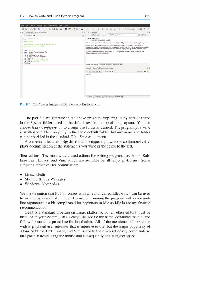
H.2 How to Write and Run a Python Program 879
Fig. H.1 The Spyder Integrated Development Environment.
The plot file we generate in the above program, tmp.png, is by default foundin the Spyder folder listed in the default text in the top of the program. You canchoose Run - Configure . . . to change this folder as desired. The program you writeis written to a file .temp.py in the same default folder, but any name and foldercan be specified in the standard File - Save as. . . menu.
A convenient feature of Spyder is that the upper right window continuously dis-plays documentation of the statements you write in the editor to the left.
Text editors The most widely used editors for writing programs are Atom, Sub-lime Text, Emacs, and Vim, which are available on all major platforms. Somesimpler alternatives for beginners are
Linux: Gedit Mac OS X: TextWrangler Windows: Notepad++
We may mention that Python comes with an editor called Idle, which can be usedto write programs on all three platforms, but running the program with command-line arguments is a bit complicated for beginners in Idle so Idle is not my favoriterecommendation.
Gedit is a standard program on Linux platforms, but all other editors must beinstalled in your system. This is easy: just google the name, download the file, andfollow the standard procedure for installation. All of the mentioned editors comewith a graphical user interface that is intuitive to use, but the major popularity ofAtom, Sublime Text, Emacs, and Vim is due to their rich set of key commands sothat you can avoid using the mouse and consequently edit at higher speed.
880 H Technical Topics
H.2.2 Terminal Windows
To run the Python program, you need a terminal window. This is a window whereyou can issue Unix commands in Linux and Mac OS X systems and DOS com-mands in Windows. On a Linux computer, gnome-terminal is my favorite, butother choices work equally well, such as xterm and konsole. On a Mac computer,launch the application Utilities - Terminal. On Windows, launch PowerShell.
You must first move to the right folder using the cd foldername command.Then running a python program prog.py is a matter of writing python prog.py.Whatever the program prints can be seen in the terminal window.
Using a plain text editor and a terminal window1. Create a folder where your Python programs can be located, say with name
mytest under your home folder. This is most conveniently done in the terminalwindow since you need to use this window anyway to run the program. Thecommand for creating a new folder is mkdir mytest.
2. Move to the new folder: cd mytest.3. Start the editor of your choice.4. Write a program in the editor, e.g., just the line print ’Hello!’. Save the
program under the name myprog1.py in the mytest folder.5. Move to the terminal window and write python myprog1.py. You should see
the word Hello! being printed in the window.
H.3 The SageMathCloud andWakari Web Services
You can avoid installing Python on your machine completely by using a web servicethat allows you to write and run Python programs. Computational science projectswill normally require some kind of visualization and associated graphics packages,which is not possible unless the service offers IPython notebooks. There are twoexcellent web services with notebooks: SageMathCloud at https://cloud.sagemath.com/ andWakari at https://www.wakari.io/wakari. At both sites you must create anaccount before you can write notebooks in the web browser and download them toyour own computer.
H.3.1 Basic Intro to SageMathCloud
Sign in, click on New Project, give a title to your project and decide whether itshould be private or public, click on the project when it appears in the browser,and click on Create or Import a File, Worksheet, Terminal or Directory. . . . If yourPython program needs graphics, you need to choose IPython Notebook, otherwiseyou can choose File. Write the name of the file above the row of buttons. As-suming we do not need any graphics, we create a plain Python file, say with namepy1.py. By clicking File you are brought to a browser window with a text editorwhere you can write Python code. Write some code and click Save. To run theprogram, click on the plus icon (New), choose Terminal, and you have a plain Unix
H.3 The SageMathCloud and Wakari Web Services 881
terminal window where you can write python py1.py to run the program. Tabsover the terminal (or editor) window make it easy to jump between the editor andthe terminal. To download the file, click on Files, point on the relevant line with thefile, and a download icon appears to the very right. The IPython notebook optionworks much in the same way, see Sect. H.4.
H.3.2 Basic Intro toWakari
After having logged in at the wakari.io site, you automatically enter an IPythonnotebook with a short introduction to how the notebook can be used. Click onthe New Notebook button to start a new notebook. Wakari enables creating andediting plain Python files too: click on the Add file icon in pane to the left, fill in theprogram name, and you enter an editor where you can write a program. PressingExecute launches an IPython session in a terminal window, where you can run theprogram by run prog.py if prog.py is the name of the program. To downloadthe file, select test2.py in the left pane and click on the Download file icon.
There is a pull-down menu where you can choose what type of terminal windowyou want: a plain Unix shell, an IPython shell, or an IPython shell with Matplotlibfor plotting. Using the latter, you can run plain Python programs or commands withgraphics. Just choose the type of terminal and click on+Tab to make a new terminalwindow of the chosen type.
H.3.3 Installing Your Own Python Packages
Both SageMathCloud and Wakari let you install your own Python packages. Toinstall any package packagename available at PyPi28, run
Terminal
pip install --user packagename
To install the SciTools package, which is useful when working with this book, runthe command
Terminal
pip install --user -e \git+https://github.com/hplgit/scitools.git#egg=scitools
28 https://pypi.python.org/pypi
882 H Technical Topics
H.4 Writing IPython Notebooks
The IPython notebook is a splendid interactive tool for doing science, but it canalso be used as a platform for developing Python code. You can either run itlocally on your computer or in a web service like SageMathCloud or Wakari. In-stallation on your computer is trivial on Ubuntu, just sudo apt-get installipython-notebook, and also on Windows and Mac29 by using Anaconda or En-thought Canopy for the Python installation.
The interface to the notebook is a web browser: you write all the code and seeall the results in the browser window. There are excellent YouTube videos on howto use the IPython notebook, so here we provide a very quick “step zero” to getanyone started.
H.4.1 A Simple Program in the Notebook
Start the IPython notebook locally by the command ipython notebook or go toSageMathCloud or Wakari as described above. The default input area is a cell forPython code. Type
g = 9.81
v0 = 5
t = 0.6
y = v0*t - 0.5*g*t**2
in a cell and run the cell by clicking on Run Selected (notebook running locallyon your machine) or on the “play” button (notebook running in the cloud). Thisaction will execute the Python code and initialize the variables g, v0, t, and y. Youcan then write print y in a new cell, execute that cell, and see the output of thisstatement in the browser. It is easy to go back to a cell, edit the code, and re-executeit.
To download the notebook to your computer, choose the File - Download asmenu and select the type of file to be downloaded: the original notebook format(.ipynb file extension) or a plain Python program version of the notebook (.py fileextension).
H.4.2 Mixing Text, Mathematics, Code, and Graphics
The real strength of IPython notebooks arises when you want to write a report todocument how a problem can be explored and solved. As a teaser, open a newnotebook, click in the first cell, and chooseMarkdown as format (notebook runninglocally) or switch from Code to Markdown in the pull-down menu (notebook inthe cloud). The cell is now a text field where you can write text with Markdown30
syntax. Mathematics can be entered as LATEX code. Try some text with inline math-ematics and an equation on a separate line:
29 http://ipython.org/install.html30 http://daringfireball.net/projects/markdown/syntax
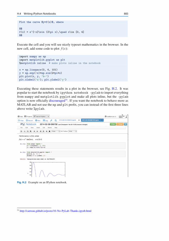
H.4 Writing IPython Notebooks 883
Plot the curve $y=f(x)$, where
$$
f(x) = e^{-x}\sin (2\pi x),\quad x\in [0, 4]
$$
Execute the cell and you will see nicely typeset mathematics in the browser. In thenew cell, add some code to plot f .x/:
import numpy as np
import matplotlib.pyplot as plt
%matplotlib inline # make plots inline in the notebook
x = np.linspace(0, 4, 101)
y = np.exp(-x)*np.sin(2*pi*x)
plt.plot(x, y, ’b-’)
plt.xlabel(’x’); plt.ylabel(’y’)
Executing these statements results in a plot in the browser, see Fig. H.2. It waspopular to start the notebook by ipython notebook –pylab to import everythingfrom numpy and matplotlib.pyplot and make all plots inline, but the –pylaboption is now officially discouraged31. If you want the notebook to behave more asMATLAB and not use the np and plt prefix, you can instead of the first three linesabove write %pylab.
Fig. H.2 Example on an IPython notebook.
31 http://carreau.github.io/posts/10-No-PyLab-Thanks.ipynb.html
884 H Technical Topics
H.5 Different Ways of Running Python Programs
Python programs are compiled and interpreted by another program called python.To run a Python program, you need to tell the operating system that your programis to be interpreted by the python program. This section explains various ways ofdoing this.
H.5.1 Executing Python Programs in iPython
The simplest and most flexible way of executing a Python program is to run it insideIPython. See Sect. 1.5.3 for a quick introduction to IPython. You start IPythoneither by the command ipython in a terminal window, or by double-clicking theIPython program icon (on Windows). Then, inside IPython, you can run a programprog.py by
In [1]: run prog.py arg1 arg2
where arg1 and arg2 are command-line arguments.This method of running Python programs works the same way on all platforms.
One additional advantage of running programs under IPython is that you can au-tomatically enter the Python debugger if an exception is raised (see Sect. F.1).Although we advocate running Python programs under IPython in this book, youcan also run them directly under specific operating systems. This is explained nextfor Unix, Windows, and Mac OS X.
H.5.2 Executing Python Programs in Unix
There are two ways of executing a Python program prog.py in Unix-based sys-tems. The first explicitly tells which Python interpreter to use:
Terminal
Unix> python prog.py arg1 arg2
Here, arg1 and arg2 are command-line arguments.There may be many Python interpreters on your computer system, usually cor-
responding to different versions of Python or different sets of additional packagesand modules. The Python interpreter (python) used in the command above is thefirst programwith the name python appearing in the folders listed in your PATH en-vironment variable. A specific python interpreter, say in /home/hpl/local/bin,can easily be used as default choice by putting this folder name first in the PATHvariable. PATH is normally controlled in the .bashrc file. Alternatively, we mayspecify the interpreter’s complete file path when running prog.py:
Terminal
Unix> /home/hpl/bin/python prog.py arg1 arg2
H.5 Different Ways of Running Python Programs 885
The other way of executing Python programs in Unix consists of just writing thename of the file:
Terminal
Unix> ./prog.py arg1 arg2
The leading ./ is needed to tell that the program is located in the current folder.You can also just write
Terminal
Unix> prog.py arg1 arg2
but then you need to have the dot in the PATH variable, which is not recommendedfor security reasons.
In the two latter commands there is no information on which Python interpreterto use. This information must be provided in the first line of the program, normallyas
#!/usr/bin/env python
This looks like a comment line, and behaves indeed as a comment line when werun the program as python prog.py. However, when we run the program as./prog.py, the first line beginning with #! tells the operating system to use theprogram specified in the rest of the first line to interpret the program. In this ex-ample, we use the first python program encountered in the folders in your PATHvariable. Alternatively, a specific python program can be specified as
#!/home/hpl/special/tricks/python
H.5.3 Executing Python Programs inWindows
In a DOS or PowerShell window you can always run a Python program by
Terminal
PowerShell> python prog.py arg1 arg2
if prog.py is the name of the program, and arg1 and arg2 are command-linearguments. The extension .py can be dropped:
Terminal
PowerShell> python prog arg1 arg2
If there are several Python installations on your system, a particular installation canbe specified:
886 H Technical Topics
Terminal
PowerShell> E:\hpl\myprogs\Python2.7.5\python prog arg1 arg2
Files with a certain extension can in Windows be associated with a file type,and a file type can be associated with a particular program to handle the file. Forexample, it is natural to associate the extension .py with Python programs. Thecorresponding program needed to interpret .py files is then python.exe. Whenwe write just the name of the Python program file, as in
Terminal
PowerShell> prog arg1 arg2
the file is always interpreted by the specified python.exe program. The details ofgetting .py files to be interpreted by python.exe go as follows:
Terminal
PowerShell> assoc .py=PyProgPowerShell> ftype PyProg=python.exe "%1" %*
Depending on your Python installation, such file extension bindings may already bedone. You can check this with
Terminal
PowerShell> assoc | find "py"
To see the programs associated with a file type, write ftype name where name isthe name of the file type as specified by the assoc command. Writing help ftypeand help assoc prints out more information about these commands along withexamples.
One can also run Python programs by writing just the basename of the pro-gram file, i.e., prog.py instead of prog.py, if the file extension is registered in thePATHEXT environment variable.
Double-clicking Python files The usual way of running programs in Windows isto double click on the file icon. This does not work well with Python programswithout a graphical user interface. When you double click on the icon for a fileprog.py, a DOS window is opened, prog.py is interpreted by some python.exeprogram, and when the program terminates, the DOS window is closed. There isusually too little time for the user to observe the output in this short-lived DOSwindow.
One can always insert a final statement that pauses the program by waiting forinput from the user:
raw_input(’Type CR:’)
H.5 Different Ways of Running Python Programs 887
or
sys.stdout.write(’Type CR:’); sys.stdin.readline()
The program will hang until the user presses the Return key. During this pause theDOS window is visible and you can watch the output from previous statements inthe program.
The downside of including a final input statement is that you must always hitReturn before the program terminates. This is inconvenient if the program is movedto a Unix-type machine. One possibility is to let this final input statement be activeonly when the program is run in Windows:
if sys.platform[:3] == ’win’:
raw_input(’Type CR:’)
Python programs that have a graphical user interface can be double-clicked inthe usual way if the file extension is .pyw.
H.5.4 Executing Python Programs in Mac OS X
Since a variant of Unix is used as core in the Mac OS X operating system, youcan always launch a Unix terminal and use the techniques from Sect. H.5.2 to runPython programs.
H.5.5 Making a Complete Stand-Alone Executable
Python programs need a Python interpreter and usually a set of modules to be in-stalled on the computer system. Sometimes this is inconvenient, for instance whenyou want to give your program to somebody who does not necessarily have Pythonor the required set of modules installed.
Fortunately, there are tools that can create a stand-alone executable program outof a Python program. This stand-alone executable can be run on every computerthat has the same type of operating system and the same chip type. Such a stand-alone executable is a bundling of the Python interpreter and the required modules,along with your program, in a single file.
The leading tool for creating a stand-alone executable (or alternatively a folderwith all necessary files) is PyInstaller32. Say you have program myprog.py thatyou want to distribute to people without the necessary Python environment on theircomputer. You run
Terminal
Terminal> pyinstaller --onefile myprog.py
32 http://www.pyinstaller.org/
888 H Technical Topics
and a folder dist is created with the (big) stand-alone executable file myprog (ormyprog.exe in Windows).
H.6 Doing Operating System Tasks in Python
Python has extensive support for operating system tasks, such as file and foldermanagement. The great advantage of doing operating system tasks in Python andnot directly in the operating system is that the Python code works uniformly onUnix/Linux, Windows, and Mac (there are exceptions, but they are few). Belowwe list some useful operations that can be done inside a Python program or in aninteractive session.
Make a folder Python applies the term directory instead of folder. The equivalentof the Unix mkdir mydir is
import os
os.mkdir(’mydir’)
Ordinary files are created by the open and close functions in Python.
Make intermediate folders Suppose you want to make a subfolder under yourhome folder:
$HOME/python/project1/temp
but the intermediate folders python and project1 do not exist. This requires eachnew folder to be made separately by os.mkdir, or you can make all folders at oncewith os.makedirs:
foldername = os.path.join(os.environ[’HOME’], ’python’,
’project1’, ’temp’)
os.makedirs(foldername)
With os.environ[var] we can get the value of any environment variable varas a string. The os.path.join function joins folder names and a filename ina platform-independent way.
Move to a folder The cd command reads os.chdir and cwd is os.getcwd:
origfolder = os.getcwd() # get name of current folder
os.chdir(foldername) # move ("change directory")
...
os.chdir(origfolder) # move back
Rename a file or folder The cross-platform mv command is
os.rename(oldname, newname)
H.6 Doing Operating System Tasks in Python 889
List files Unix wildcard notation can be used to list files. The equivalent of ls*.py and ls plot*[1-4]*.dat reads
import glob
filelist1 = glob.glob(’*.py’)
filelist2 = glob.glob(’plot*[1-4]*.dat’)
List all files and folders in a folder The counterparts to ls -a mydir and justls -a are
filelist1 = os.listdir(’mydir’)
filelist1 = os.listdir(os.curdir) # current folder (directory)
filelist1.sort() # sort alphabetically
Check if a file or folder exists The widely used constructions in Unix scripts fortesting if a file or folder exist are if [ -f $filename ]; then and if [ -d$dirname ]; then. These have very readable counterparts in Python:
if os.path.isfile(filename):
inputfile = open(filename, ’r’)
...
if os.path.isdir(dirnamename):
filelist = os.listdir(dirname)
...
Remove files Removing a single file is done with os.rename, and a loop is re-quired for doing rm tmp_*.df:
import glob
filelist = glob.glob(’tmp_*.pdf’)
for filename in filelist:
os.remove(filename)
Remove a folder and all its subfolders The rm -rf mytree command removesan entire folder tree. In Python, the cross-platform valid command becomes
import shutil
shutil.rmtree(foldername)
It goes without saying that this command must be used with great care!
Copy a file to another file or folder The cp fromfile tofile construction ap-plies shutil.copy in Python:
shutil.copy(’fromfile’, ’tofile’)
890 H Technical Topics
Copy a folder and all its subfolders The recursive copy command cp -r forfolder trees is in Python expressed by shell.copytree:
shutil.copytree(sourcefolder, destination)
Run any operating system command The simplest way of running another pro-gram from Python is to use os.system:
cmd = ’python myprog.py 21 --mass 4’ # command to be run
failure = os.system(cmd)
if failure:
print ’Execution of "%s" failed!\n’ % cmd
sys.exit(1)
The recommended way to run operating system commands is to use thesubprocessmodule. The above command is equivalent to
import subprocess
cmd = ’python myprog.py 21 --mass 4’
failure = subprocess.call(cmd, shell=True)
# or
failure = subprocess.call(
[’python’, ’myprog.py’, ’21’, ’--mass’, ’4’])
The output of an operating system command can be stored in a string object:
try:
output = subprocess.check_output(cmd, shell=True,
stderr=subprocess.STDOUT)
except subprocess.CalledProcessError as e:
# Raise a more informative exception
msg = ’Execution of "%s" failed! (error code: %s)’ + \
’\nOutput: %s’ % (cmd, e.returncode, e.output)
raise subprocess.CalledProcessError(msg)
# or do sys.exit(1)
# Process output
for line in output.splitlines():
...
The stderr argument ensures that the output string contains everything that thecommand cmd wrote to both standard output and standard error.
The constructions above are mainly used for running stand-alone programs. Anyfile or folder listing or manipulation should be done by the functionality in the osand shutilmodules.
Split file or folder name Given data/file1.dat as a file path relative to thehome folder /users/me ($HOME/data/file1.dat in Unix). Python has tools forextracting the complete folder name /users/me/data, the basename file1.dat,and the extension .dat:
H.7 Variable Number of Function Arguments 891
>>> path = os.path.join(os.environ[’HOME’], ’data’, ’file1.dat’)
>>> path
’/users/me/data/file1.dat’
>>> foldername, basename = os.path.split(path)
>>> foldername
’/users/me/data’
>>> basename
’file1.dat’
>>> stem, ext = os.path.splitext(basename)
>>> stem
’file1’
>>> ext
’.dat’
>>> outfile = stem + ’.out’
>>> outfile
’file1.out’
H.7 Variable Number of Function Arguments
Arguments to Python functions are of four types:
positional arguments, where each argument has a name, keyword arguments, where each argument has a name and a default value, a variable number of positional arguments, where each argument has no name,
but just a location in a list, a variable number of keyword arguments, where each argument is a name-value
pair in a dictionary.
The corresponding general function definition can be sketched as
def f(pos1, pos2, key1=val1, key2=val2, *args, **kwargs):
Here, pos1 and pos2 are positional arguments, key1 and key2 are keyword ar-guments, args is a tuple holding a variable number of positional arguments, andkwargs is a dictionary holding a variable number of keyword arguments. This ap-pendix describes how to program with the args and kwargs variables and whythese are handy in many situations.
H.7.1 Variable Number of Positional Arguments
Let us start by making a function that takes an arbitrary number of arguments andcomputes their sum:
>>> def add(*args):
... print ’args:’, args
... s = 0
... for arg in args:
... s = s + arg
892 H Technical Topics
... return s
...
>>> add(1)
args: (1,)
1
>>> add(1,5,10)
args: (1, 5, 10)
16
We observe that args is a tuple and that all the arguments we provide in a call toadd are stored in args.
Combination of ordinary positional arguments and a variable number of argu-ments is allowed, but the *args argument must appear after the ordinary positionalarguments, e.g.,
def f(pos1, pos2, pos3, *args):
In each call to f we must provide at least three arguments. If more arguments aresupplied in the call, these are collected in the args tuple inside the f function.
Example Consider a mathematical function with one independent variable t anda parameter v0, as in y.t I v0/ D v0t � 1
2gt2. A more general case with n parameters
is f .xI p1; : : : ; pn/. The Python implementation of such functions can take boththe independent variable and the parameters as arguments: y(t, v0) and f(x,p1, p2, ...,pn). Suppose that we have a general library routine that operateson functions of one variable. The routine can, e.g., perform numerical differentia-tion, integration, or root finding. A simple example is a numerical differentiationfunction
def diff(f, x, h):
return (f(x+h) - f(x))/h
This diff function cannot be used with functions f that take more than one argu-ment. For example, passing an y(t, v0) function as f leads to the exception
TypeError: y() takes exactly 2 arguments (1 given)
Section 7.1.1 provides a solution to this problem where y becomes a class instance.Here we shall describe an alternative solution that allows our y(t, v0) function tobe used as is.
The idea is that we pass additional arguments for the parameters in the f functionthrough the diff function. That is, we view the f function as f(x, *f_prms) indiff. Our diff routine can then be written as
def diff(f, x, h, *f_prms):
print ’x:’, x, ’h:’, h, ’f_prms:’, f_prms
return (f(x+h, *f_prms) - f(x, *f_prms))/h
Before explaining this function in detail, we demonstrate that it works in an exam-ple:
H.7 Variable Number of Function Arguments 893
def y(t, v0):
g = 9.81
return v0*t - 0.5*g*t**2
dydt = diff(y, 0.1, 1E-9, 3) # t=0.1, h=1E-9, v0=3
The output from the call to diff becomes
x: 0.1 h: 1e-09 f_prms: (3,)
The point is that the v0 parameter, which we want to pass on to our y function, isnow stored in f_prms. Inside the diff function, calling
f(x, *f_prms)
is the same as if we had written
f(x, f_prms[0], f_prms[1], ...)
That is, *f_prms in a call takes all the values in the tuple *f_prms and places themafter each other as positional arguments. In the present example with the y function,f(x, *f_prms) implies f(x, f_prms[0]), which for the current set of argumentvalues in our example becomes a call y(0.1, 3).
For a function with many parameters,
def G(x, t, A, a, w):
return A*exp(-a*t)*sin(w*x)
the output from
dGdx = diff(G, 0.5, 1E-9, 0, 1, 0.6, 100)
becomes
x: 0.5 h: 1e-09 f_prms: (0, 1, 1.5, 100)
We pass here the arguments t, A, a, and w, in that sequence, as the last four argu-ments to diff, and all the values are stored in the f_prms tuple.
The diff function also works for a plain function f with one argument:
from math import sin
mycos = diff(sin, 0, 1E-9)
In this case, *f_prms becomes an empty tuple, and a call like f(x, *f_prms) isjust f(x).
The use of a variable set of arguments for sending problem-specific parametersthrough a general library function, as we have demonstrated here with the difffunction, is perhaps the most frequent use of *args-type arguments.
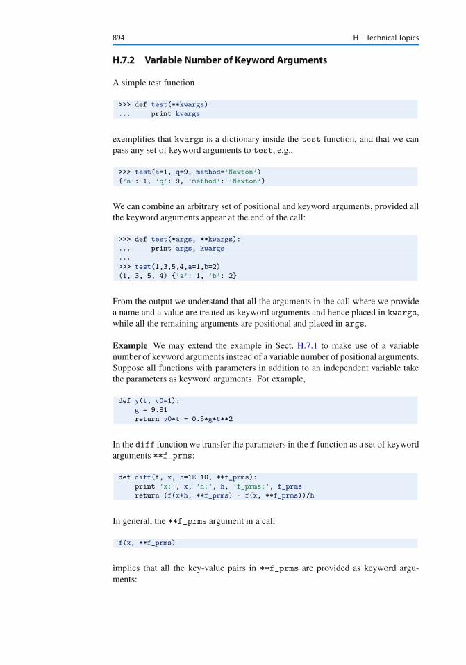
894 H Technical Topics
H.7.2 Variable Number of Keyword Arguments
A simple test function
>>> def test(**kwargs):
... print kwargs
exemplifies that kwargs is a dictionary inside the test function, and that we canpass any set of keyword arguments to test, e.g.,
>>> test(a=1, q=9, method=’Newton’)
{’a’: 1, ’q’: 9, ’method’: ’Newton’}
We can combine an arbitrary set of positional and keyword arguments, provided allthe keyword arguments appear at the end of the call:
>>> def test(*args, **kwargs):
... print args, kwargs
...
>>> test(1,3,5,4,a=1,b=2)
(1, 3, 5, 4) {’a’: 1, ’b’: 2}
From the output we understand that all the arguments in the call where we providea name and a value are treated as keyword arguments and hence placed in kwargs,while all the remaining arguments are positional and placed in args.
Example We may extend the example in Sect. H.7.1 to make use of a variablenumber of keyword arguments instead of a variable number of positional arguments.Suppose all functions with parameters in addition to an independent variable takethe parameters as keyword arguments. For example,
def y(t, v0=1):
g = 9.81
return v0*t - 0.5*g*t**2
In the diff function we transfer the parameters in the f function as a set of keywordarguments **f_prms:
def diff(f, x, h=1E-10, **f_prms):
print ’x:’, x, ’h:’, h, ’f_prms:’, f_prms
return (f(x+h, **f_prms) - f(x, **f_prms))/h
In general, the **f_prms argument in a call
f(x, **f_prms)
implies that all the key-value pairs in **f_prms are provided as keyword argu-ments:
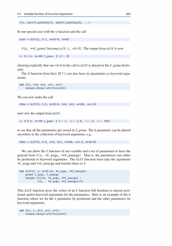
H.7 Variable Number of Function Arguments 895
f(x, key1=f_prms[key1], key2=f_prms[key2], ...)
In our special case with the y function and the call
dydt = diff(y, 0.1, h=1E-9, v0=3)
f(x, **f_prms) becomes y(0.1, v0=3). The output from diff is now
x: 0.1 h: 1e-09 f_prms: {’v0’: 3}
showing explicitly that our v0=3 in the call to diff is placed in the f_prms dictio-nary.
The G function from Sect. H.7.1 can also have its parameters as keyword argu-ments:
def G(x, t=0, A=1, a=1, w=1):
return A*exp(-a*t)*sin(w*x)
We can now make the call
dGdx = diff(G, 0.5, h=1E-9, t=0, A=1, w=100, a=1.5)
and view the output from diff,
x: 0.5 h: 1e-09 f_prms: {’A’: 1, ’a’: 1.5, ’t’: 0, ’w’: 100}
to see that all the parameters get stored in f_prms. The h parameter can be placedanywhere in the collection of keyword arguments, e.g.,
dGdx = diff(G, 0.5, t=0, A=1, w=100, a=1.5, h=1E-9)
We can allow the f function of one variable and a set of parameters to have thegeneral form f(x, *f_args, **f_kwargs). That is, the parameters can eitherbe positional or keyword arguments. The diff function must take the arguments*f_args and **f_kwargs and transfer these to f:
def diff(f, x, h=1E-10, *f_args, **f_kwargs):
print f_args, f_kwargs
return (f(x+h, *f_args, **f_kwargs) -
f(x, *f_args, **f_kwargs))/h
This diff function gives the writer of an f function full freedom to choose posi-tional and/or keyword arguments for the parameters. Here is an example of the Gfunction where we let the t parameter be positional and the other parameters bekeyword arguments:
def G(x, t, A=1, a=1, w=1):
return A*exp(-a*t)*sin(w*x)
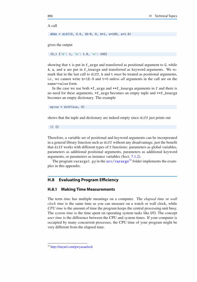
896 H Technical Topics
A call
dGdx = diff(G, 0.5, 1E-9, 0, A=1, w=100, a=1.5)
gives the output
(0,) {’A’: 1, ’a’: 1.5, ’w’: 100}
showing that t is put in f_args and transferred as positional argument to G, whileA, a, and w are put in f_kwargs and transferred as keyword arguments. We re-mark that in the last call to diff, h and t must be treated as positional arguments,i.e., we cannot write h=1E-9 and t=0 unless all arguments in the call are on thename=value form.
In the case we use both *f_args and **f_kwargs arguments in f and there isno need for these arguments, *f_args becomes an empty tuple and **f_kwargsbecomes an empty dictionary. The example
mycos = diff(sin, 0)
shows that the tuple and dictionary are indeed empty since diff just prints out
() {}
Therefore, a variable set of positional and keyword arguments can be incorporatedin a general library function such as diffwithout any disadvantage, just the benefitthat diff works with different types of f functions: parameters as global variables,parameters as additional positional arguments, parameters as additional keywordarguments, or parameters as instance variables (Sect. 7.1.2).
The program varargs1.py in the src/varargs33 folder implements the exam-ples in this appendix.
H.8 Evaluating Program Efficiency
H.8.1 Making TimeMeasurements
The term time has multiple meanings on a computer. The elapsed time or wallclock time is the same time as you can measure on a watch or wall clock, whileCPU time is the amount of time the program keeps the central processing unit busy.The system time is the time spent on operating system tasks like I/O. The conceptuser time is the difference between the CPU and system times. If your computer isoccupied by many concurrent processes, the CPU time of your program might bevery different from the elapsed time.
33 http://tinyurl.com/pwyasaa/tech
H.8 Evaluating Program Efficiency 897
The time module Python has a timemodule with some useful functions for mea-suring the elapsed time and the CPU time:
import time
e0 = time.time() # elapsed time since the epoch
c0 = time.clock() # total CPU time spent in the program so far
<do tasks...>
elapsed_time = time.time() - e0
cpu_time = time.clock() - c0
The term epoch means initial time (time.time() would return 0), which is00:00:00 January 1, 1970. The time module also has numerous functions fornice formatting of dates and time, and the newer datetimemodule has more func-tionality and an improved interface. Although the timing has a finer resolution thanseconds, one should construct test cases that last some seconds to obtain reliableresults.
Using timeit from IPython To measure the efficiency of a certain set of state-ments, an expression, or a function call, the code should be run a large number oftimes so the overall CPU time is of order seconds. Python’s timeit module hasfunctionality for running a code segment repeatedly. The simplest and most conve-nient way of using timeit is within an IPython shell. Here is a session comparingthe efficiency of sin(1.2) versus math.sin(1.2):
In [1]: import math
In [2]: from math import sin
In [3]: %timeit sin(1.2)
10000000 loops, best of 3: 198 ns per loop
In [4]: %timeit math.sin(1.2)
1000000 loops, best of 3: 258 ns per loop
That is, looking up sin through the math prefix degrades the performance by a fac-tor of 258=198 � 1:3.
Any statement, including function calls, can be timed the same way. Timing ofmultiple statements is possible by using %%timeit. The timeit module can beused inside ordinary programs as demonstrated in the file pow_eff.py.
Hardware information Along with CPU time measurements it is often conve-nient to print out information about the hardware on which the experiment wasdone. Python has a module platform with information on the current hardware.The function scitools.misc.hardware_info applies the platformmodule andother modules to extract relevant hardware information. A sample call is
>>> import scitools.misc, pprint
>>> pprint.pprint(scitools.misc.hardware_info())
{’numpy.distutils.cpuinfo.cpu.info’: [
{’address sizes’: ’40 bits physical, 48 bits virtual’,
898 H Technical Topics
’bogomips’: ’4598.87’,
’cache size’: ’4096 KB’,
’cache_alignment’: ’64’,
’cpu MHz’: ’2299.435’,
...
},
’platform module’: {
’identifier’: ’Linux-3.11.0-12-generic-x86_64-with-Ubuntu-13.10’,
’python build’: (’default’, ’Sep 19 2013 13:48:49’),
’python version’: ’2.7.5+’,
’uname’: (’Linux’, ’hpl-ubuntu2-mac11’, ’3.11.0-12-generic’,
’#19-Ubuntu SMP Wed Oct 9 16:20:46 UTC 2013’,
’x86_64’, ’x86_64’)}}
}
H.8.2 Profiling Python Programs
A profiler computes the time spent in the various functions of a program. From thetimings a ranked list of the most time-consuming functions can be created. This isan indispensable tool for detecting bottlenecks in the code, and you should alwaysperform a profiling before spending time on code optimization. The golden rule isto first write an easy-to-understand program, then verify it, then profile it, and thenthink about optimization.
I Premature optimization is the root of all evil.Donald Knuth, computer scientist, 1938–.
Python 2.7 comes with two recommended profilers, implemented in the mod-ules cProfile and profiles. The section The Python Profilers34 in the PythonStandard Library documentation [3] has a good introduction to the usage of thesemodules. The results produced by the modules are normally processed by a spe-cial statistics utility pstats developed for analyzing profiling results. The usageof the profile, cProfile, and pstats modules is straightforward, but some-what tedious. The SciTools package therefore comes with a command scitoolsprofiler that allows you to profile any program (say) m.py by just writing
Terminal
Terminal> scitools profiler m.py c1 c2 c3
Here, c1, c2, and c3 are command-line arguments to m.py.A sample output might read
1082 function calls (728 primitive calls) in 17.890 CPU s
Ordered by: internal time
List reduced from 210 to 20 due to restriction <20>
34 http://docs.python.org/2/library/profile.html
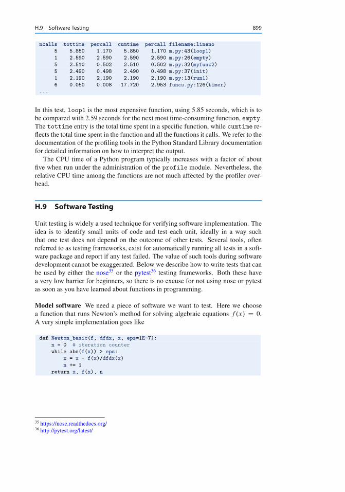
H.9 Software Testing 899
ncalls tottime percall cumtime percall filename:lineno
5 5.850 1.170 5.850 1.170 m.py:43(loop1)
1 2.590 2.590 2.590 2.590 m.py:26(empty)
5 2.510 0.502 2.510 0.502 m.py:32(myfunc2)
5 2.490 0.498 2.490 0.498 m.py:37(init)
1 2.190 2.190 2.190 2.190 m.py:13(run1)
6 0.050 0.008 17.720 2.953 funcs.py:126(timer)
...
In this test, loop1 is the most expensive function, using 5.85 seconds, which is tobe compared with 2.59 seconds for the next most time-consuming function, empty.The tottime entry is the total time spent in a specific function, while cumtime re-flects the total time spent in the function and all the functions it calls. We refer to thedocumentation of the profiling tools in the Python Standard Library documentationfor detailed information on how to interpret the output.
The CPU time of a Python program typically increases with a factor of aboutfive when run under the administration of the profile module. Nevertheless, therelative CPU time among the functions are not much affected by the profiler over-head.
H.9 Software Testing
Unit testing is widely a used technique for verifying software implementation. Theidea is to identify small units of code and test each unit, ideally in a way suchthat one test does not depend on the outcome of other tests. Several tools, oftenreferred to as testing frameworks, exist for automatically running all tests in a soft-ware package and report if any test failed. The value of such tools during softwaredevelopment cannot be exaggerated. Below we describe how to write tests that canbe used by either the nose35 or the pytest36 testing frameworks. Both these havea very low barrier for beginners, so there is no excuse for not using nose or pytestas soon as you have learned about functions in programming.
Model software We need a piece of software we want to test. Here we choosea function that runs Newton’s method for solving algebraic equations f .x/ D 0.A very simple implementation goes like
def Newton_basic(f, dfdx, x, eps=1E-7):
n = 0 # iteration counter
while abs(f(x)) > eps:
x = x - f(x)/dfdx(x)
n += 1
return x, f(x), n
35 https://nose.readthedocs.org/36 http://pytest.org/latest/
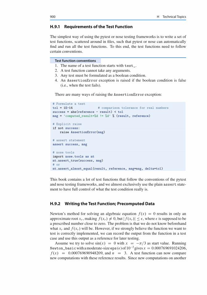
900 H Technical Topics
H.9.1 Requirements of the Test Function
The simplest way of using the pytest or nose testing frameworks is to write a set oftest functions, scattered around in files, such that pytest or nose can automaticallyfind and run all the test functions. To this end, the test functions need to followcertain conventions.
Test function conventions1. The name of a test function starts with test_.2. A test function cannot take any arguments.3. Any test must be formulated as a boolean condition.4. An AssertionError exception is raised if the boolean condition is false
(i.e., when the test fails).
There are many ways of raising the AssertionError exception:
# Formulate a test
tol = 1E-14 # comparison tolerance for real numbers
success = abs(reference - result) < tol
msg = ’computed_result=%d != %d’ % (result, reference)
# Explicit raise
if not success:
raise AssertionError(msg)
# assert statement
assert success, msg
# nose tools
import nose.tools as nt
nt.assert_true(success, msg)
# or
nt.assert_almost_equal(result, reference, msg=msg, delta=tol)
This book contains a lot of test functions that follow the conventions of the pytestand nose testing frameworks, and we almost exclusively use the plain assert state-ment to have full control of what the test condition really is.
H.9.2 Writing the Test Function; Precomputed Data
Newton’s method for solving an algebraic equation f .x/ D 0 results in only anapproximate root xr , making f .xr/ ¤ 0, but jf .xr/j � �, where � is supposed to bea prescribed number close to zero. The problem is that we do not know beforehandwhat xr and f .xr / will be. However, if we strongly believe the function we want totest is correctly implemented, we can record the output from the function in a testcase and use this output as a reference for later testing.
Assume we try to solve sin.x/ D 0 with x D ��=3 as start value. RunningNewton_basicwithamoderate-sizeeps (�)of10�2givesx D 0:000769691024206,f .x/ D 0:000769690948209, and n D 3. A test function can now comparenew computations with these reference results. Since new computations on another
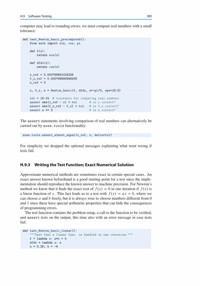
H.9 Software Testing 901
computer may lead to rounding errors, we must compare real numbers with a smalltolerance:
def test_Newton_basic_precomputed():
from math import sin, cos, pi
def f(x):
return sin(x)
def dfdx(x):
return cos(x)
x_ref = 0.000769691024206
f_x_ref = 0.000769690948209
n_ref = 3
x, f_x, n = Newton_basic(f, dfdx, x=-pi/3, eps=1E-2)
tol = 1E-15 # tolerance for comparing real numbers
assert abs(x_ref - x) < tol # is x correct?
assert abs(f_x_ref - f_x) < tol # is f_x correct?
assert n == 3 # is n correct?
The assert statements involving comparison of real numbers can alternatively becarried out by nose.tools functionality:
nose.tools.assert_almost_equal(x_ref, x, delta=tol)
For simplicity we dropped the optional messages explaining what went wrong iftests fail.
H.9.3 Writing the Test Function; Exact Numerical Solution
Approximate numerical methods are sometimes exact in certain special cases. Anexact answer known beforehand is a good starting point for a test since the imple-mentation should reproduce the known answer to machine precision. For Newton’smethod we know that it finds the exact root of f .x/ D 0 in one iteration if f .x/ isa linear function of x. This fact leads us to a test with f .x/ D ax C b, where wecan choose a and b freely, but it is always wise to choose numbers different from 0and 1 since these have special arithmetic properties that can hide the consequencesof programming errors.
The test function contains the problem setup, a call to the function to be verified,and assert tests on the output, this time also with an error message in case testsfail:
def test_Newton_basic_linear():
"""Test that a linear func. is handled in one iteration."""
f = lambda x: a*x + b
dfdx = lambda x: a
a = 0.25; b = -4
902 H Technical Topics
x_exact = 16
eps = 1E-5
x, f_x, n = Newton_basic(f, dfdx, -100, eps)
tol = 1E-15 # tolerance for comparing real numbers
assert abs(x - 16) < tol, ’wrong root x=%g != 16’ % x
assert abs(f_x) < eps, ’|f(root)|=%g > %g’ % (f_x, eps)
assert n == 1, ’n=%d, but linear f should have n=1’ % n
H.9.4 Testing of Function Robustness
Our Newton_basic function is very basic and suffers from several problems:
for divergent iterations it will iterate forever, it can divide by zero in f(x)/dfdx(x), it can perform integer division in f(x)/dfdx(x), it does not test whether the arguments have acceptable types and values.
A more robust implementation dealing with these potential problems look as fol-lows:
def Newton(f, dfdx, x, eps=1E-7, maxit=100):
if not callable(f):
raise TypeError(
’f is %s, should be function or class with __call__’
% type(f))
if not callable(dfdx):
raise TypeError(
’dfdx is %s, should be function or class with __call__’
% type(dfdx))
if not isinstance(maxit, int):
raise TypeError(’maxit is %s, must be int’ % type(maxit))
if maxit <= 0:
raise ValueError(’maxit=%d <= 0, must be > 0’ % maxit)
n = 0 # iteration counter
while abs(f(x)) > eps and n < maxit:
try:
x = x - f(x)/float(dfdx(x))
except ZeroDivisionError:
raise ZeroDivisionError(
’dfdx(%g)=%g - cannot divide by zero’ % (x, dfdx(x)))
n += 1
return x, f(x), n
The numerical functionality can be tested as described in the previous example,but we should include additional tests for testing the additional functionality. Onecan have different tests in different test functions, or collect several tests in one testfunction. The preferred strategy depends on the problem. Here it may be natural tohave different test functions only when the f .x/ formula differs to avoid repeatingcode.
H.9 Software Testing 903
To test for divergence, we can choose f .x/ D tanh.x/, which is known to leadto divergent iterations if not x is sufficiently close to the root x D 0. A start valuex D 20 reveals that the iterations are divergent, so we set maxit=12 and test thatthe actual number of iterations reaches this limit. We can also add a test on x, e.g.,that x is a big as we know it will be: x > 1050 after 12 iterations. The test functionbecomes
def test_Newton_divergence():
from math import tanh
f = tanh
dfdx = lambda x: 10./(1 + x**2)
x, f_x, n = Newton(f, dfdx, 20, eps=1E-4, maxit=12)
assert n == 12
assert x > 1E+50
To test for division by zero, we can find an f .x/ and an x such that f 0.x/ D0. One simple example is x D 0, f .x/ D cos.x/, and f 0.x/ D � sin.x/. Ifx D 0 is the start value, we know that a division by zero will take place in the firstiteration, and this will lead to a ZeroDivisionError exception. We can explicitlyhandle this exception and introduce a boolean variable success that is True if theexception is raised and otherwise False. The corresponding test function reads
def test_Newton_div_by_zero1():
from math import sin, cos
f = cos
dfdx = lambda x: -sin(x)
success = False
try:
x, f_x, n = Newton(f, dfdx, 0, eps=1E-4, maxit=1)
except ZeroDivisionError:
success = True
assert success
There is a special nose.tools.assert_raises helper function that can beused to test if a function raises a certain exception. The arguments to assert_raises are the exception type, the name of the function to be called, and all posi-tional and keyword arguments in the function call:
import nose.tools as nt
def test_Newton_div_by_zero2():
from math import sin, cos
f = cos
dfdx = lambda x: -sin(x)
nt.assert_raises(
ZeroDivisionError, Newton, f, dfdx, 0, eps=1E-4, maxit=1)
Let us proceed with testing that wrong input is caught by function Newton. Sincethe same type of exception is raised for different type of errors we shall now alsoexamine (parts of) the exception messages. The first test involves an argument fthat is not a function:
904 H Technical Topics
def test_Newton_f_is_not_callable():
success = False
try:
Newton(4.2, ’string’, 1.2, eps=1E-7, maxit=100)
except TypeError as e:
if "f is <type ’float’>" in e.message:
success = True
As seen, success = True demands that the right exception is raised and that itsmessage starts with f is <type ’float’>. What text to expect in the message isevident from the source in function Newton.
The nose.toolsmodule also has a function for testing the exception type andthe message content. This is illustrated when dfdx is not callable:
def test_Newton_dfdx_is_not_callable():
nt.assert_raises_regexp(
TypeError, "dfdx is <type ’str’>", Newton,
lambda x: x**2, ’string’, 1.2, eps=1E-7, maxit=100)
Checking that Newton catches maxit of wrong type or with a negative value canbe carried out by these test functions:
def test_Newton_maxit_is_not_int():
nt.assert_raises_regexp(
TypeError, "maxit is <type ’float’>",
Newton, lambda x: x**2, lambda x: 2*x,
1.2, eps=1E-7, maxit=1.2)
def test_Newton_maxit_is_neg():
nt.assert_raises_regexp(
ValueError, "maxit=-2 <= 0",
Newton, lambda x: x**2, lambda x: 2*x,
1.2, eps=1E-7, maxit=-2)
The corresponding support for testing exceptions in pytest is
import pytest
with pytest.raises(TypeError) as e:
Newton(lambda x: x**2, lambda x: 2*x, 1.2, eps=1E-7, maxit=-2)
H.9.5 Automatic Execution of Tests
Our code for the Newton_basic and Newton functions is placed in a file eq_solver.py together with the tests. To run all test functions with names of theform test_*() in this file, use the nosetests or py.test commands, e.g.:
H.9 Software Testing 905
Terminal
Terminal> nosetests -s eq_solver.py..........-------------------------------------------------------------------Ran 10 tests in 0.004s
OK
The -s option causes all output from the called functions in the program eq_solver.py to appear on the screen (by default, nosetests and py.test suppressall output). The final OK points to the fact that no test failed. Adding the option-v prints out the outcome of each individual test function. In case of failure, theAssertionError exception and the associated message, if existing, are displayed.Pytest also displays the code that failed.
WarningDo not use more than one period in the names of files with test functions(e.g., avoid names like ex7.23.py). Also, do not use hyphens in the name of(sub)directories. Both constructions confuse nosetests and py.test.
One can also collect test functions in separate files with names starting withtest. A simple command nosetests -s -v will look for all such files in thisfolder as well as in all subfolders if the folder names start with test or end with_test or _tests. By following this naming convention, nosetests can auto-matically run a potentially large number of tests and give us quick feedback. Thepy.test -s -v command will look for and run all test files in the entire tree ofany subfolder.
Remark on classical class-based unit testingThe pytest and nose testing frameworks allow ordinary functions, as explainedabove, to perform the testing. The most widespread way of implementing unittests, however, is to use class-based frameworks. This is also possible with noseand with a module unittest that comes with standard Python. The class-basedapproach is very accessible for people with experience from JUnit in Java andsimilar tools in other languages. Without such a background, plain functionsthat follow the pytest/nose conventions are faster and cleaner to write than theclass-based counterparts.
References
1. D. Beazley. Python Essential Reference. Addison-Wesley, 4th edition, 2009.
2. O. Certik et al. SymPy: Python library for symbolic mathematics. http://sympy.org/.
3. Python Software Foundation. The Python standard library. http://docs.python.org/2/library/.
4. C. Führer, J. E. Solem, and O. Verdier. Computing with Python - An Introduction to Pythonfor Science and Engineering. Pearson, 2014.
5. J. E. Grayson. Python and Tkinter Programming. Manning, 2000.
6. Richard Gruet. Python quick reference. http://rgruet.free.fr/.
7. D. Harms and K. McDonald. The Quick Python Book. Manning, 1999.
8. J. D. Hunter. Matplotlib: a 2d graphics environment. Computing in Science & Engineering, 9,2007.
9. J. D. Hunter et al. Matplotlib: Software package for 2d graphics. http://matplotlib.org/.
10. E. Jones, T. E. Oliphant, P. Peterson, et al. SciPy scientific computing library for Python. http://scipy.org.
11. D. E. Knuth. Theory and practice. EATCS Bull., 27:14–21, 1985.
12. H. P. Langtangen. Quick intro to version control systems and project hosting sites. http://hplgit.github.io/teamods/bitgit/html/.
13. H. P. Langtangen. Python Scripting for Computational Science, volume 3 of Texts in Compu-tational Science and Engineering. Springer, 3rd edition, 2009.
14. H. P. Langtangen and J. H. Ring. SciTools: Software tools for scientific computing. http://code.google.com/p/scitools.
15. L. S. Lerner. Physics for Scientists and Engineers. Jones and Barlett, 1996.
16. M. Lutz. Programming Python. O’Reilly, 4th edition, 2011.
17. M. Lutz. Learning Python. O’Reilly, 2013.
18. J. D. Murray. Mathematical Biology I: an Introduction. Springer, 3rd edition, 2007.
19. T. E. Oliphant. Python for scientific computing. Computing in Science & Engineering, 9, 2007.
20. T. E. Oliphant et al. NumPy array processing package for Python. http://www.numpy.org.
21. F. Perez and B. E. Granger. IPython: a system for interactive scientific computing. Computingin Science & Engineering, 9, 2007.
22. F. Perez, B. E. Granger, et al. IPython software package for interactive scientific computing.http://ipython.org/.
23. Python programming language. http://python.org.
24. G. J. E. Rawlins. Slaves of the Machine: The Quickening of Computer Technology. MIT Press,1998.
25. G. Ward and A. Baxter. Distributing Python modules. http://docs.python.org/2/distutils/.
26. F. M. White. Fluid Mechanics. McGraw-Hill, 2nd edition, 1986.
907
Index
%, 530**kwargs, 894*=, 54*args, 891+=, 54/=, 54-=, 54
Aallclose in numpy, 448allocate, 236animate, 540API, 457aplotter (from scitools), 255append (list), 58application, 12application programming interface, 457argparse module, 162array (from numpy), 234array (datatype), 233array computing, 233array shape, 271, 277array slicing, 234asarray (from numpy), 269assert statement, 120, 126, 192, 193, 431,
434, 448, 761AssertionError, 193Atom, 879attribute (class), 414average, 494
Bbackend (Easyviz), 245, 247base class, 568Bernoulli trials, 224bin (histogram), 492binomial distribution, 224bioinformatics, 113bits, 176blank lines in files, 354
blanks, 15body of a function, 92boolean expressions, 54boolean indexing, 264, 265break statement, 168bytes, 176
Ccall a function, 92callable objects, 432callback function, 740check an object’s type, 26, 270, 458, 571check file/folder existence (in Python), 889class hierarchy, 567class relationship
derived class, 568has-a, 572inheritance, 568is-a, 572subclass, 568superclass, 568
closure, 424, 435, 436, 587cmath module, 31command-line arguments, 151commands module, 890comments, 8comparing
floating-point numbers, 87objects, 87real numbers, 87
complex numbers, 29concatenate (from numpy), 667console (terminal) window, 4constructor (class), 412continue statement, 400convergence rate, 640, 815convert program, 540copy files (in Python), 889copy folders (in Python), 890CPU time measurements, 119, 896
909
910 Index
cross (from numpy), 283cumulative sum, 556curve plotting, 238
Ddate object, 348date conversion, 348datetime module, 340, 348, 648debugger demo, 835debugging, 838del, 58delete files (in Python), 253, 680, 889delete folders (in Python), 889derived class, 568determinant, 283dictionary, 333, 377
comprehensions, 338functionality, 396nested, 343
difference equations, 645nonlinear, 664
differential equations, 715, 757, 772, 833dir function, 462directory, 1, 4, 888DNA, 113doc strings, 105dot (from numpy), 283dtype, 269duck typing, 460dynamic binding, 578dynamic typing, 459
Eefficiency, 896efficiency measure, 533eigenvalues, 283eigenvectors, 283elapsed time, 896Emacs, 879endswith (string method), 353enumerate function, 66, 376, 480environment variables, 888eval function, 154, 581event loop, 187except, 179Exception, 183exceptions, 179, 839execute programs (from Python), 890execute Python program, 4, 27, 884expression, 14
Ffactorial function, 56, 138factory function, 582find (string method), 352first-order ODEs, 724Flake8, 853
f.__name__ (name of func. f), 120format (string method), 11format string syntax, 11formatting text and numbers, 9Forward Euler instability, 788Forward Euler scheme, 759Fourier series, 136frequency matrix, 375function arguments
keyword, 103named, 103positional, 103
function body, 92function header, 92function inside function, 783functional programming, 587
GGaussian function, 45Gedit, 879global, 96globals function, 95, 260, 746globals(), 580glob.glob function, 680, 889grid, 684
Hhas-a class relationship, 572Heaviside function, 139heterogeneous lists, 233histogram (normalized), 492
IIdle, 879immutable objects, 336, 445IndexError, 179, 181, 182, 840information hiding, 457initial condition, 645, 716, 735in-place array arithmetics, 268input (data), 15insert (list), 58instance (class), 413integer random numbers, 497integration
numerical, 438symbolic, 439
interactive sessionsIPython, 27standard Python shell, 24
interpolation, 321interval arithmetic, 466inverse, 283invoke a function, 92IPython, 27
command history, 28executing operating system commands, 27running Python programs, 27
Index 911
start-up file, 27is, 102is-a class relationship, 572isdigit (string method), 354isinstance function, 75, 270, 458, 571isspace (string method), 354
Jjoin, 153, 355
Kkeys (dictionaries), 334keyword arguments, 103, 891
LLagrange’s interpolation formula, 321lambda functions, 110, 113lambdify (in sympy), 34Leapfrog method for ODEs, 779least squares approximation, 317len (list), 58line break, 11linspace (from numpy), 234, 271Linux, 15list comprehension, 66, 67, 116list files (in Python), 889list functionality, 75list iteration, 114list, nested, 67lists, 57logical expressions, 54loops, 52lower (string method), 353lstrip (string method), 354
MMac OS X, 15main program, 109make a folder (in Python), 888making graphs, 238making movie, 540math module, 21matrix (mat) object, 277, 282max (from numpy), 284, 380mean (from numpy), 494, 495, 543measure time in programs, 533mesh, 684method (class), 60, 414Midpoint method for ODEs, 779, 814Midpoint method w/iterations for ODEs, 780,
815Midpoint rule for integration, 131, 329, 527,
587, 592, 640, 675, 841mod function, 126, 494, 530module folders, 197modules, 188Monte Carlo integration, 526
Monte Carlo simulation, 507move to a folder (in Python), 888multiple inheritance, 639mutable objects, 336, 445
Nnamed arguments, 103NameError, 182, 839namespace, 422nested dictionaries, 343nested lists, 67nested loops, 72newline character (line break), 11new-style classes, 416Newton’s method, 435, 659None, 102non-English characters, 8nonlinear difference equations, 664normal (from numpy.random), 496normally distributed random numbers, 496norms in numpy, 284nose package, 761nose tests, 120, 126, 192, 431, 899nosetests command, 904not, 54Notepad++, 879np prefix (numpy), 234np.array function, 234np.linspace function, 234np.zeros function, 234np.zeros_like function, 234Numerical Python, 233NumPy, 233numpy, 233numpy.lib.scimath module, 31
Oobject, inheritance from, 416object-based programming, 567object-oriented programming, 642objects, 17ODE, 715, 757Online Python Tutor, 93, 127, 571operating system (OS), 15optimization of Python code, 898option-value pairs (command line), 161OrderDict class, 339ordinary differential equations, 715, 757, 833os module, 888os.chdir function, 888oscillating systems, 724, 731, 737, 797os.listdir function, 889os.makedirs function, 888os.mkdir function, 888os.pardir, 198os.path.isdir function, 889os.path.isfile function, 889
912 Index
os.path.join function, 197, 888os.path.split function, 890os.remove function, 253, 680, 889os.rename function, 888os.system function, 890output (data), 15overloading (of methods), 591
Pparent class, 568pass, 456PATH environment variable, 198PEP8, 41, 853plot (from scitools), 245plotting, 238plotting data vs date, 348Poisson distribution, 224Poisson process, 224polymorphism, 591positional arguments, 103, 891pprint2 (from scitools), 69pprint.pformat, 69pprint.pprint, 69pretty print, 69printf syntax, 9private attributes (class), 457probability, 507profiler.py script, 898profiling, 898protected attributes (class), 445, 457pydoc program, 81PyLint, 853pysketcher, 599py.test command, 904pytest tests, 120, 126, 192, 431, 899PYTHONPATH environment variable, 198
Rr_ (array creation), 271raise, 183randint (from numpy.random), 537randn (from numpy.random), 496random module, 489, 493random numbers, 489
histogram, 492integers, 497integration, 526Monte Carlo simulation, 507normal distribution, 496random walk, 534statistics, 494uniform distribution, 491vectorization, 493
random strings, 118random walk, 534random_integers (from numpy.random),
537
random.normalvariate function, 496rank of a matrix, 288raw_input function, 150recursive function calls, 614refactoring, 212remove files (in Python), 253, 680, 889remove folders (in Python), 889rename file/folder (in Python), 888replace (string method), 353resolution (mesh), 684round function, 26rounding errors, 23rounding float to integer, 26rstrip (string method), 354run programs (from Python), 890run Python program, 4, 27, 884
Sscalar (math quantity), 229scalar code, 237scalar differential equation, 724, 758scalar function, 758scaling, 653scitools.pprint2 module, 69scitools.std, 244search for module files, 197Secant method, 674second-order ODEs, 724, 734, 797seed, 490sequence (data type), 76sequence (mathematical), 645shape (of an array), 271, 277shutil.copy function, 889shutil.copytree function, 890shutil.rmtree function, 889slicing, 70, 351software testing
nose, 899pytest, 899
sort (list), 144source code, 12special methods (class), 432split (string method), 353split filename, 890splitlines (string method), 353spread of a disease (model), 727standard deviation, 494standard error, 174standard input, 173standard output, 173startswith (string method), 353statements, 13static class attributes, 463static class methods, 463static class variables, 463static typing, 459std (from numpy), 495, 543
Index 913
str2obj (from scitools), 204string, 9
case change, 353find, 352joining words, 355replace, 353searching, 352splitting, 353stripping leading/trailing blanks, 354substitution, 353substrings, 351testing for number, 354
string iteration, 114string slicing, 351StringFunction (from scitools), 160strip (string method), 354strong typing, 459subarrays, 234subclass, 568Sublime Text, 879sublist, 70subprocess module, 890substitution (in text), 353substrings, 351sum, 116, 117, 284, 337, 498sum (˙ ) implementation, 77summing a list, 337summing over an iterator, 337superclass, 568symbolic computing, 439SymPy, 33
differentiation, 33, 436equation solving, 34integration, 33, 439Taylor series, 35
sympy, 33, 439syntax, 14SyntaxError, 182, 839sys module, 151sys.argv, 151sys.exit function, 179sys.path, 197sys.stderr, 174sys.stdin, 173sys.stdout, 173system time, 896systems of differential equations, 724, 772
Tterminal window, 4test block (in module files), 190test function, 120, 126, 192, 431, 434, 448,
761test_*() function, 120, 126, 192, 212, 431,
434, 448, 761, 767, 852TextWrangler, 879time module, 88, 121, 533, 535, 896
CPU, 896elapsed, 896system, 896user, 896
timeit, 897timing utilities, 896transpose (in numpy), 286Trapezoidal rule for integration, 130, 318, 330,
589, 592, 640, 655triple-quoted strings, 10try, 179tuples, 74type function, 26, 75type conversion, 26TypeError, 182, 840
UUML class diagram, 412uniform (from numpy.random), 493uniformly distributed random numbers, 491unit testing, 126, 192, 899Unix, 15upper (string method), 353urllib, 387user (of a program), 15user time, 896user-defined datatype (class), 413using a debugger, 835
VValueError, 181, 182, 840var (from numpy), 495, 543variable no. of function arguments, 891variance, 494vector computing, 229vectorization, 233, 236vectorized drawing of random numbers, 493vectors, 228verification, 849Vim, 879
Wweak typing, 459where (from numpy), 263whitespace, 15, 354widgets, 186Windows, 15with statement, 167wrap2callable, 763wrapper code, 438
Xxrange function, 236, 498
ZZeroDivisionError, 182zeros (from numpy), 234

914 Index
zeros_like (from numpy), 234zip function, 66
zombies, 821
Editorial Policy
§1. Textbooks on topics in the field of computational science and engineering willbe considered. They should be written for courses in CSE education. Both graduateand undergraduate textbooks will be published in TCSE. Multidisciplinary topicsand multidisciplinary teams of authors are especially welcome.
§2. Format: Only works in English will be considered. For evaluation pur-poses, manuscripts may be submitted in print or electronic form, in the latter case,preferably as pdf- or zipped ps-files. Authors are requested to use the LaTeX stylefiles available fromSpringer at: https://www.springer.com/gp/authors-editors/book-authors-editors/manuscript-preparation/5636 (Click on �! Templates �! LaTeX�! monographs)Electronic material can be included if appropriate. Please contact the publisher.
§3. Those considering a book which might be suitable for the series are stronglyadvised to contact the publisher or the series editors at an early stage.
General Remarks
Careful preparation of manuscripts will help keep production time short and ensurea satisfactory appearance of the finished book.
The following terms and conditions hold:
Regarding free copies and royalties, the standard terms for Springer mathematicstextbooks hold. Please write to [email protected] for details.
Authors are entitled to purchase further copies of their book and other Springerbooks for their personal use, at a discount of 33.3% directly from Springer-Verlag.

Series Editors
Timothy J. BarthNASA Ames Research CenterNAS DivisionMoffett Field, CA 94035, [email protected]
Michael GriebelInstitut für Numerische Simulationder Universität BonnWegelerstr. 653115 Bonn, [email protected]
David E. KeyesMathematical and Computer Sciencesand EngineeringKing Abdullah University of Scienceand TechnologyP.O. Box 55455Jeddah 21534, Saudi [email protected]
and
Department of Applied Physicsand Applied MathematicsColumbia University500 W. 120 th StreetNew York, NY 10027, [email protected]
Risto M. NieminenDepartment of Applied PhysicsAalto University School of Scienceand Technology00076 Aalto, [email protected]
Dirk RooseDepartment of Computer ScienceKatholieke Universiteit LeuvenCelestijnenlaan 200A3001 Leuven-Heverlee, [email protected]
Tamar SchlickDepartment of Chemistryand Courant Instituteof Mathematical SciencesNew York University251 Mercer StreetNew York, NY 10012, [email protected]
Editor for Computational Scienceand Engineering at Springer:Martin PetersSpringer-VerlagMathematics Editorial IVTiergartenstrasse 1769121 Heidelberg, [email protected]
Texts in Computational Scienceand Engineering
1. H. P. Langtangen, Computational Partial Differential Equations. Numerical Methods and DiffpackProgramming. 2nd Edition
2. A. Quarteroni, F. Saleri, P. Gervasio, Scientific Computing with MATLAB and Octave. 4th Edition
3. H. P. Langtangen, Python Scripting for Computational Science. 3rd Edition
4. H. Gardner, G. Manduchi, Design Patterns for e-Science.
5. M. Griebel, S. Knapek, G. Zumbusch, Numerical Simulation in Molecular Dynamics.
6. H. P. Langtangen, A Primer on Scientific Programming with Python. 5th Edition
7. A. Tveito, H. P. Langtangen, B. F. Nielsen, X. Cai, Elements of Scientific Computing.
8. B. Gustafsson, Fundamentals of Scientific Computing.
9. M. Bader, Space-Filling Curves.
10. M. Larson, F. Bengzon, The Finite Element Method: Theory, Implementation and Applications.
11. W. Gander, M. Gander, F. Kwok, Scientific Computing: An Introduction using Maple and MATLAB.
12. P. Deuflhard, S. Röblitz, A Guide to Numerical Modelling in Systems Biology.
13. M. H. Holmes, Introduction to Scientific Computing and Data Analysis.
14. S. Linge, H. P. Langtangen, Programming for Computations – A Gentle Introduction to NumericalSimulations with MATLAB/Octave.
15. S. Linge, H. P. Langtangen, Programming for Computations – A Gentle Introduction to NumericalSimulations with Python.
For further information on these books please have a look at our mathematics catalogue at the following
URL: www.springer.com/series/5151
Monographs in Computational Scienceand Engineering
1. J. Sundnes, G.T. Lines, X. Cai, B.F. Nielsen, K.-A. Mardal, A. Tveito, Computing the ElectricalActivity in the Heart.
For further information on this book, please have a look at our mathematics catalogue at the following
URL: www.springer.com/series/7417
Lecture Notesin Computational Scienceand Engineering
1. D. Funaro, Spectral Elements for Transport-Dominated Equations.
2. H.P. Langtangen, Computational Partial Differential Equations. Numerical Methods and DiffpackProgramming.
3. W. Hackbusch, G. Wittum (eds.),Multigrid Methods V.
4. P. Deuflhard, J. Hermans, B. Leimkuhler, A.E. Mark, S. Reich, R.D. Skeel (eds.), ComputationalMolecular Dynamics: Challenges, Methods, Ideas.
5. D. Kröner, M. Ohlberger, C. Rohde (eds.), An Introduction to Recent Developments in Theory andNumerics for Conservation Laws.
6. S. Turek, Efficient Solvers for Incompressible Flow Problems. An Algorithmic and ComputationalApproach.
7. R. von Schwerin, Multi Body System SIMulation. Numerical Methods, Algorithms, and Software.
8. H.-J. Bungartz, F. Durst, C. Zenger (eds.), High Performance Scientific and Engineering Comput-ing.
9. T.J. Barth, H. Deconinck (eds.), High-Order Methods for Computational Physics.
10. H.P. Langtangen, A.M. Bruaset, E.Quak (eds.),Advances in Software Tools for Scientific Comput-ing.
11. B. Cockburn, G.E. Karniadakis, C.-W. Shu (eds.), Discontinuous Galerkin Methods. Theory, Com-putation and Applications.
12. U. van Rienen, Numerical Methods in Computational Electrodynamics. Linear Systems in PracticalApplications.
13. B. Engquist, L. Johnsson, M. Hammill, F. Short (eds.), Simulation and Visualization on the Grid.
14. E. Dick, K. Riemslagh, J. Vierendeels (eds.), Multigrid Methods VI.
15. A. Frommer, T. Lippert, B. Medeke, K. Schilling (eds.), Numerical Challenges in Lattice QuantumChromodynamics.
16. J. Lang, Adaptive Multilevel Solution of Nonlinear Parabolic PDE Systems. Theory, Algorithm,and Applications.
17. B.I. Wohlmuth, Discretization Methods and Iterative Solvers Based on Domain Decomposition.
18. U. van Rienen, M. Günther, D. Hecht (eds.), Scientific Computing in Electrical Engineering.
19. I. Babuška, P.G. Ciarlet, T. Miyoshi (eds.), Mathematical Modeling and Numerical Simulation inContinuum Mechanics.
20. T.J. Barth, T. Chan, R. Haimes (eds.), Multiscale and Multiresolution Methods. Theory andApplications.
21. M. Breuer, F. Durst, C. Zenger (eds.), High Performance Scientific and Engineering Computing.
22. K. Urban, Wavelets in Numerical Simulation. Problem Adapted Construction and Applications.
23. L.F. Pavarino, A. Toselli (eds.), Recent Developments in Domain Decomposition Methods.
24. T. Schlick, H.H. Gan (eds.), Computational Methods for Macromolecules: Challenges andApplications.
25. T.J. Barth, H. Deconinck (eds.), Error Estimation and Adaptive Discretization Methods inComputational Fluid Dynamics.
26. M. Griebel, M.A. Schweitzer (eds.), Meshfree Methods for Partial Differential Equations.
27. S. Müller, Adaptive Multiscale Schemes for Conservation Laws.
28. C. Carstensen, S. Funken, W. Hackbusch, R.H.W. Hoppe, P. Monk (eds.), ComputationalElectromagnetics.
29. M.A. Schweitzer, A Parallel Multilevel Partition of Unity Method for Elliptic Partial DifferentialEquations.
30. T. Biegler, O. Ghattas, M. Heinkenschloss, B. van Bloemen Waanders (eds.), Large-Scale PDE-Constrained Optimization.
31. M. Ainsworth, P. Davies, D. Duncan, P. Martin, B. Rynne (eds.), Topics in Computational WavePropagation. Direct and Inverse Problems.
32. H. Emmerich, B. Nestler, M. Schreckenberg (eds.), Interface and Transport Dynamics. Computa-tional Modelling.
33. H.P. Langtangen, A. Tveito (eds.), Advanced Topics in Computational Partial DifferentialEquations. Numerical Methods and Diffpack Programming.
34. V. John, Large Eddy Simulation of Turbulent Incompressible Flows. Analytical and NumericalResults for a Class of LES Models.
35. E. Bänsch (ed.), Challenges in Scientific Computing – CISC 2002.
36. B.N. Khoromskij, G. Wittum, Numerical Solution of Elliptic Differential Equations by Reductionto the Interface.
37. A. Iske, Multiresolution Methods in Scattered Data Modelling.
38. S.-I. Niculescu, K. Gu (eds.), Advances in Time-Delay Systems.
39. S. Attinger, P. Koumoutsakos (eds.), Multiscale Modelling and Simulation.
40. R. Kornhuber, R. Hoppe, J. Périaux, O. Pironneau, O. Wildlund, J. Xu (eds.), Domain Decomposi-tion Methods in Science and Engineering.
41. T. Plewa, T. Linde, V.G. Weirs (eds.), Adaptive Mesh Refinement – Theory and Applications.
42. A. Schmidt, K.G. Siebert, Design of Adaptive Finite Element Software. The Finite Element ToolboxALBERTA.
43. M. Griebel, M.A. Schweitzer (eds.), Meshfree Methods for Partial Differential Equations II.
44. B. Engquist, P. Lötstedt, O. Runborg (eds.),Multiscale Methods in Science and Engineering.
45. P. Benner, V. Mehrmann, D.C. Sorensen (eds.), Dimension Reduction of Large-Scale Systems.
46. D. Kressner, Numerical Methods for General and Structured Eigenvalue Problems.
47. A. Boriçi, A. Frommer, B. Joó, A. Kennedy, B. Pendleton (eds.), QCD and Numerical Analysis III.
48. F. Graziani (ed.), Computational Methods in Transport.
49. B. Leimkuhler, C. Chipot, R. Elber, A. Laaksonen, A. Mark, T. Schlick, C. Schütte, R. Skeel (eds.),New Algorithms for Macromolecular Simulation.
50. M. Bücker, G. Corliss, P. Hovland, U. Naumann, B. Norris (eds.), Automatic Differentiation: Ap-plications, Theory, and Implementations.
51. A.M. Bruaset, A. Tveito (eds.), Numerical Solution of Partial Differential Equations on ParallelComputers.
52. K.H. Hoffmann, A. Meyer (eds.), Parallel Algorithms and Cluster Computing.
53. H.-J. Bungartz, M. Schäfer (eds.), Fluid-Structure Interaction.
54. J. Behrens, Adaptive Atmospheric Modeling.
55. O. Widlund, D. Keyes (eds.), Domain Decomposition Methods in Science and Engineering XVI.
56. S. Kassinos, C. Langer, G. Iaccarino, P. Moin (eds.), Complex Effects in Large Eddy Simulations.
57. M. Griebel, M.A Schweitzer (eds.), Meshfree Methods for Partial Differential Equations III.
58. A.N. Gorban, B. Kégl, D.C. Wunsch, A. Zinovyev (eds.), Principal Manifolds for Data Visualiza-tion and Dimension Reduction.
59. H. Ammari (ed.), Modeling and Computations in Electromagnetics: A Volume Dedicated to Jean-Claude Nédélec.
60. U. Langer, M. Discacciati, D. Keyes, O. Widlund, W. Zulehner (eds.), Domain DecompositionMethods in Science and Engineering XVII.
61. T. Mathew, Domain Decomposition Methods for the Numerical Solution of Partial DifferentialEquations.
62. F. Graziani (ed.), Computational Methods in Transport: Verification and Validation.
63. M. Bebendorf, Hierarchical Matrices. A Means to Efficiently Solve Elliptic Boundary ValueProblems.
64. C.H. Bischof, H.M. Bücker, P. Hovland, U. Naumann, J. Utke (eds.), Advances in AutomaticDifferentiation.
65. M. Griebel, M.A. Schweitzer (eds.),Meshfree Methods for Partial Differential Equations IV.
66. B. Engquist, P. Lötstedt, O. Runborg (eds.), Multiscale Modeling and Simulation in Science.
67. I.H. Tuncer, Ü. Gülcat, D.R. Emerson, K. Matsuno (eds.), Parallel Computational Fluid Dynamics2007.
68. S. Yip, T. Diaz de la Rubia (eds.), Scientific Modeling and Simulations.
69. A. Hegarty, N. Kopteva, E. O’Riordan, M. Stynes (eds.), BAIL 2008 – Boundary and InteriorLayers.
70. M. Bercovier, M.J. Gander, R. Kornhuber, O. Widlund (eds.), Domain Decomposition Methods inScience and Engineering XVIII.
71. B. Koren, C. Vuik (eds.), Advanced Computational Methods in Science and Engineering.
72. M. Peters (ed.), Computational Fluid Dynamics for Sport Simulation.
73. H.-J. Bungartz, M. Mehl, M. Schäfer (eds.), Fluid Structure Interaction II – Modelling, Simulation,Optimization.
74. D. Tromeur-Dervout, G. Brenner, D.R. Emerson, J. Erhel (eds.), Parallel Computational FluidDynamics 2008.
75. A.N. Gorban, D. Roose (eds.), Coping with Complexity: Model Reduction and Data Analysis.
76. J.S. Hesthaven, E.M. Rønquist (eds.), Spectral and High Order Methods for Partial DifferentialEquations.
77. M. Holtz, Sparse Grid Quadrature in High Dimensions with Applications in Finance and Insur-ance.
78. Y. Huang, R. Kornhuber, O.Widlund, J. Xu (eds.), Domain Decomposition Methods in Science andEngineering XIX.
79. M. Griebel, M.A. Schweitzer (eds.),Meshfree Methods for Partial Differential Equations V.
80. P.H. Lauritzen, C. Jablonowski, M.A. Taylor, R.D. Nair (eds.), Numerical Techniques for GlobalAtmospheric Models.
81. C. Clavero, J.L. Gracia, F.J. Lisbona (eds.), BAIL 2010 – Boundary and Interior Layers, Computa-tional and Asymptotic Methods.
82. B. Engquist, O. Runborg, Y.R. Tsai (eds.), Numerical Analysis and Multiscale Computations.
83. I.G. Graham, T.Y. Hou, O. Lakkis, R. Scheichl (eds.), Numerical Analysis of Multiscale Problems.
84. A. Logg, K.-A. Mardal, G. Wells (eds.), Automated Solution of Differential Equations by the FiniteElement Method.
85. J. Blowey, M. Jensen (eds.), Frontiers in Numerical Analysis – Durham 2010.
86. O. Kolditz, U.-J. Gorke, H. Shao, W.Wang (eds.), Thermo-Hydro-Mechanical-Chemical Processesin Fractured Porous Media – Benchmarks and Examples.
87. S. Forth, P. Hovland, E. Phipps, J. Utke, A. Walther (eds.), Recent Advances in Algorithmic Differ-entiation.
88. J. Garcke, M. Griebel (eds.), Sparse Grids and Applications.
89. M. Griebel, M.A. Schweitzer (eds.), Meshfree Methods for Partial Differential Equations VI.
90. C. Pechstein, Finite and Boundary Element Tearing and Interconnecting Solvers for MultiscaleProblems.
91. R. Bank, M. Holst, O. Widlund, J. Xu (eds.), Domain Decomposition Methods in Science andEngineering XX.
92. H. Bijl, D. Lucor, S. Mishra, C. Schwab (eds.), Uncertainty Quantification in Computational FluidDynamics.
93. M. Bader, H.-J. Bungartz, T. Weinzierl (eds.), Advanced Computing.
94. M. Ehrhardt, T. Koprucki (eds.), Advanced Mathematical Models and Numerical Techniques forMulti-Band Effective Mass Approximations.
95. M. Azaïez, H. El Fekih, J.S. Hesthaven (eds.), Spectral and High Order Methods for Partial Dif-ferential Equations ICOSAHOM 2012.
96. F. Graziani, M.P. Desjarlais, R. Redmer, S.B. Trickey (eds.), Frontiers and Challenges in WarmDense Matter.
97. J. Garcke, D. Pflüger (eds.), Sparse Grids and Applications – Munich 2012.
98. J. Erhel, M. Gander, L. Halpern, G. Pichot, T. Sassi, O. Widlund (eds.), Domain DecompositionMethods in Science and Engineering XXI.
99. R. Abgrall, H. Beaugendre, P.M. Congedo, C. Dobrzynski, V. Perrier, M. Ricchiuto (eds.), HighOrder Nonlinear Numerical Methods for Evolutionary PDEs – HONOM 2013.
100. M. Griebel, M.A. Schweitzer (eds.), Meshfree Methods for Partial Differential Equations VII.
101. R. Hoppe (ed.), Optimization with PDE Constraints – OPTPDE 2014.
102. S. Dahlke, W. Dahmen, M. Griebel, W. Hackbusch, K. Ritter, R. Schneider, C. Schwab,H. Yserentant (eds.), Extraction of Quantifiable Information from Complex Systems.
103. A. Abdulle, S. Deparis, D. Kressner, F. Nobile, M. Picasso (eds.), Numerical Mathematics andAdvanced Applications – ENUMATH 2013.
104. T. Dickopf, M.J. Gander, L. Halpern, R. Krause, L.F. Pavarino (eds.), Domain DecompositionMethods in Science and Engineering XXII.
105. M. Mehl, M. Bischoff, M. Schäfer (eds.), Recent Trends in Computational Engineering – CE2014.Optimization, Uncertainty, Parallel Algorithms, Coupled and Complex Problems.
106. R.M. Kirby, M. Berzins, J.S. Hesthaven (eds.), Spectral and High Order Methods for Partial Dif-ferential Equations – ICOSAHOM’14.

107. B. Jüttler, B. Simeon (eds.), Isogeometric Analysis and Applications 2014.
108. P. Knobloch (ed.), Boundary and Interior Layers, Computational and Asymptotic Methods – BAIL2014.
109. J. Garcke, D. Pflüger (eds.), Sparse Grids and Applications – Stuttgart 2014.
110. H.P. Langtangen, Finite Difference Computing with Exponential Decay Models.
111. A. Tveito, G.T. Lines, Computing Characterizations of Drugs for Ion Channels and ReceptorsUsing Markov Models
For further information on these books please have a look at our mathematics catalogue at the following
URL: www.springer.com/series/3527