RENEWAL SEQUENCES AND INTERMITTENCY

Stefano Isola

Dipartimento di Matematica, Universita degli Studi di Bologna,

piazza di Porta S.Donato 5, I-40127 Bologna, Italy.

e-mail: isola@dm.unibo.it

Abstract. In this paper we examine the generating function Φ(z) of a renewal

sequence arising from the distribution of return times in the ‘turbulent’ region

for a class of piecewise affine interval maps introduced by Gaspard and Wang(1)

and studied by several authors(2−8). We prove that it admits a meromorphic

continuation to the entire complex z-plane with a branch cut along the ray

(1,+∞). Moreover we compute the asymptotic behaviour of the coefficients of

its Taylor expansion at z = 0. From this, the exact polynomial asympotics for

the rate of mixing when the invariant measure is finite and of the scaling rate

when it is infinite are obtained.

1

0. INTRODUCTION.

The Pomeau-Manneville(9) type 1 intermittency model (at the tangent bifurca-

tion point) consists of a class of smooth transformations f : [0, 1] → [0, 1] which

are expanding everywhere but at a neutral fixed point at the origin. Such inter-

mittent interval maps provide with no doubt the simplest examples of ‘chaotic’

dynamical systems with anomalous statistical behaviour. For instance they may

possess but a σ-finite non-normalizable invariant measure(10−12). Or else, they

may leave invariant a probability measure with slow (e.g. polynomial) speed

of mixing(14−16). Finally, in the framework of thermodynamic formalism, they

may exhibit phase transitions(6−8) and dynamical ζ-functions with non-polar

singularities(14,18).

Here we consider a one parameter family of linearized intermittent interval maps

(see eq.(1.2) below) introduced by Gaspard and Wang(1,2). As far as its statis-

tical properties are concerned, it is equivalent to a Markov chain with countable

state space(13). It is also related to the statistical mechanics model introduced

by Fisher(17) and successively studied by Gallavotti(18) (see also Hofbauer(19)).

Without pretending to be a typical example, the main advantage of this approx-

imation scheme is that it partially allows for exact calculations.

The main concern of this paper is the study of the generating function of a

renewal sequence arising from the distribution of return times in a region where

the map is uniformly expanding. This function coincides, up to a factor (1−z)−1,

with the Ruelle dynamical ζ-function, and is shown to admit a meromorphic

continuation to the the entire complex z-plane with a branch cut along the ray

(1,+∞). It appears that finding analytic continuation of dynamically defined

functions, which are holomorphic in a domain given a priori, can be a rewarding

mathematical achievement in itself. Moreover, it will be shown that the main

statistical features of this dynamical system such as the rate of mixing or the

scaling rate, are embodied in the behaviour of its Taylor coefficients.

2

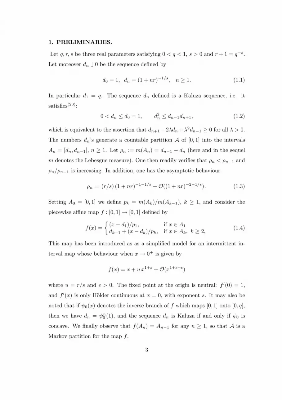
1. PRELIMINARIES.

Let q, r, s be three real parameters satisfying 0 < q < 1, s > 0 and r + 1 = q−s.

Let moreover dn ↓ 0 be the sequence defined by

d0 = 1, dn = (1 + nr)−1/s, n ≥ 1. (1.1)

In particular d1 = q. The sequence dn defined is a Kaluza sequence, i.e. it

satisfies(20):

0 < dn ≤ d0 = 1, d2n ≤ dn−1dn+1, (1.2)

which is equivalent to the assertion that dn+1−2λdn +λ2dn−1 ≥ 0 for all λ > 0.

The numbers dn’s generate a countable partition A of [0, 1] into the intervals

An = [dn, dn−1], n ≥ 1. Let ρn := m(An) = dn−1 − dn (here and in the sequel

m denotes the Lebesgue measure). One then readily verifies that ρn < ρn−1 and

ρn/ρn−1 is increasing. In addition, one has the asymptotic behaviour

ρn = (r/s) (1 + nr)−1−1/s + O((1 + nr)−2−1/s) . (1.3)

Setting A0 = [0, 1] we define pk = m(Ak)/m(Ak−1), k ≥ 1, and consider the

piecewise affine map f : [0, 1] → [0, 1] defined by

f(x) =

(x − d1)/p1, if x ∈ A1

dk−1 + (x − dk)/pk, if x ∈ Ak, k ≥ 2, (1.4)

This map has been introduced as as a simplified model for an intermittent in-

terval map whose behaviour when x → 0+ is given by

f(x) = x + u x1+s + O(x1+s+ε)

where u = r/s and ε > 0. The fixed point at the origin is neutral: f ′(0) = 1,

and f ′(x) is only Holder continuous at x = 0, with exponent s. It may also be

noted that if ψ0(x) denotes the inverse branch of f which maps [0, 1] onto [0, q],

then we have dn = ψn0 (1), and the sequence dn is Kaluza if and only if ψ0 is

concave. We finally observe that f(An) = An−1 for any n ≥ 1, so that A is a

Markov partition for the map f .

3

A countable Markov chain. One can say more: the iteration process xn =

fn(x), with f as above and x randomly chosen according to Lebesgue measure, is

actually isomorphic (mod 0) to a Markov chain with state space IN and transition

matrix P = (pij) given by

P =

ρ1 ρ2 ρ3 . . .1 0 0 . . .0 1 0 . . .0 0 1 . . ....

......

. . .

(1.5)

To see this, let X be the residual set of points in (0, 1] which are not preimages

of 1 with respect to the map f , namely X = (0, 1] \ dnn≥0. Let moreover Ω

be the set of all one-sided sequences ω = (ω0ω1 . . .), ωi ∈ IN s.t. given ωi then

ωi−1 = ωi + 1 or ωi−1 = 1. Then the map ϕ : Ω → [0, 1] defined by

ϕ(ω) = x according to f j(x) ∈ Aωj , j ≥ 0

is a bijection between Ω and X and conjugates the map f with the shift T

on Ω. It is then immediate to check that the stochastic process on Ω given

by xi(ω) = ωi, i ≥ 0, is a Markov chain with conditional probabilities pij =

P (xn(ω) = j |xn−1(ω) = i) = m(f−1(Aj)⋂

Ai)/m(Ai), which coincide with

those in (1.5). Since g.c.d.n : ρn > 0 = 1 the chain is aperiodic and recurrent.

Consider the infinite sequence t1, t2, . . . of successive entrance times in the state

1: t1 = infi ≥ 0 : ωi = 1 and, for j ≥ 2, tj = infi > tj−1 : ωi = 1. Let

moreover rj = tj+1 − tj be the sequence of times between returns. The state

1 being recurrent, the numbers rj are i.i.d.r.v. under the probability P1(·) =

P ( · |x0(ω) = 1). Their common distribution is P1(rj = n) = ρn and their

expectation value is given by E1(rj) =∑

n ρn =∑

dn, which may be finite

(positive-recurrent chain) or infinite (null-recurrent chain) according whether

s < 1 or s ≥ 1. More specifically, we can define a family of moments

M () = E1(rj) ≡

∑n ρn, ≥ 0, (1.6)

4

and say that the chain has ergodic degree if M () < ∞ but M (+1) = ∞. Notice

that M (0) = 1, so that the chain has degree at least zero (null-recurrent case).

Finally, the steady-state equation is πn =∑

i∈S πi pin and is formally solved by

πn = π1 dn−1, n ≥ 1. In the positive-recurrent case one finds π1 = (∑

dn)−1.

For more details on this Markov chain we refer to Isola(13).

Invariant measure and return times. An easy consequence of the previous

discussion is that the map f preserves an absolutely continuous σ-finite measure

ν, whose density e is given by

e(x) = πn/(ρnπ1) = dn−1/ρn, dn < x ≤ dn−1. (1.7)

It may be noted that

ν(An) = dn−1 =∑l≥n

m(Al). (1.8)

More specifically, for E ⊆ An we have, using (1.7),

ν(E) =m(E)m(An)

dn−1. (1.9)

Let τ : X → IN be the first passage time in the interval A1, that is

τ(x) = 1 + minn ≥ 0 : fn(x) ∈ A1 , (1.10)

so that An is the closure of the set x ∈ X : τ(x) = n. On the other hand, the

return time function r : X → IN in the interval A1 is given by

r(x) = minn ≥ 1 : fn(x) ∈ A1 = τ f(x). (1.11)

Let Bn = closure of x ∈ A1 : r(x) = n. Clearly Bn = A1 ∩ f−1An, and

therefore, using (1.9), we get

ν(Bn) =m(A1 ∩ f−1An)

m(A1)= m(An) (1.12)

as one can easily check. Putting togheter (1.8) and (1.12) we have the following

chain of formal identities:

ν([0, 1]) =∑

ν(An) =∑

n m(An) =∫ 1

0

τ(x) m(dx)

=∑

n

n ν(Bn) =∫

A1

r(x) ν(dx) = M (1),(1.13)

5

which is a version of Kac’s formula. Clearly (1.13) becomes meaningful under the

assumption that all terms involved are finite. Using the shorthand M ≡ M (1)

we then have the following dichotomy: either M < ∞, and then there exists

an f -invariant a.c. probability measure µ = ν/M ; or M = ∞ so that ν is not

normalizable and no invariant a.c. probability measure exists. In the latter case,

the ergodic means 1n

∑n−1k=0 δfk(x) converge weakly to the Dirac delta at 0(21,11).

For later use, we now define recursively a family of formal ‘tail sequences’ d()n ,

with ≥ 0, derived from dn as follows:

d(0)n = dn and d()

n =∑l>n

d(−1)l for > 0. (1.14)

Moreover we say that an and bn are asymptotically equivalent as n approaches

∞, denoted as an ∼ bn (n → ∞), if the quotient an/bn tends to unity. From

(1.1) (see also (1.3)) we have that if s < 1/, with ≥ 1, then the terms d(k)n are

finite for 0 ≤ k ≤ and satisfy

d(k)n ∼ (1 + (n + k)r)k− 1

s . (1.15)

It is also easy to check that M () is finite if and only if d()n is. Of special

importance will be the asymptotic behaviour of d(1)n , when s < 1:

d(1)n−1 = ν (x ∈ X : τ(x) > n) ∼ C n1− 1

s (1.16)

where C = r1− 1s .

2. THE GENERATING FUNCTION OF THE RETURN TIMES

DISTRIBUTION.

If we view the element An of the countable Markov partition A introduced in

Section 1 as the n-th ’state’ for our dynamical system, the number ρn can be

interpreted as the m-probability that a first passage in the state 1 occurs after

n iterates. Let us now consider the quantity un := m(f−(n−1)A1) which, for

6

n ≥ 1, gives the m-probability to observe a passage in the state 1 after n − 1

iterates (for the first time or not). We can write

un =n∑

r=1

ρ(f l(x) /∈ A1, 0 ≤ l < r − 1, fr−1(x) ∈ A1, fn−1(x) ∈ A1

)

=n∑

r=1

ρ (τ(x) = r) ρ(fn−1(x) ∈ A1 | τ(x) = r

)

=n∑

r=1

ρr ρ(fn−1(x) ∈ A1 | τ(x) = r

).

On the other hand, according to the discussion given in the previous Section,

the iteration process xn = fn(x) ‘starts afresh’ at each passage in the state 1.

This implies

ρ(fn−1(x) ∈ A1 | τ(x) = r

)= ρ

(fn−1(x) ∈ A1 |fr−1(x) ∈ A1

)= ρ

(fn−r(x) ∈ A1 |x ∈ A1

)= ρ

(fn−r−1(x) ∈ A1

)= un−r,

and therefore the sequence u0, u1, . . . satisfies the recurrence relation:

u0 = 1 and un = ρn + u1 ρn−1 · · · + un−1 ρ1 for n ≥ 1. (2.1)

In other words, u0, u1, . . . is the renewal sequence(20) associated with the se-

quence ρ1, ρ2, . . .. We now show that un is also equal to ν(A1 ∩ f−nA1), and

can thus be interpreted as the ν-probability to observe a return in the state 1

after n iterates (recall that ν(A1) = 1). Indeed, setting u(1)n := ν(A1 ∩ f−nA1)

and reasoning as above, we see that u(1)n satisfies the recurrence relation:

u(1)0 = 1 and u(1)

n = u(1)0 ν(Bn) + · · · + u

(1)n−1 ν(B1) for n ≥ 1, (2.2)

where Bn is defined after (1.11). On the other hand we know that ν(Bn) =

m(An) ≡ ρn and, comparing with (2.1), we get u(1)n ≡ un, ∀n.

We now turn to the study of the generating function Φ(z) of the sequence un,

which is given by

Φ(z) =∞∑

n=0

unzn =

(1 −

∞∑n=1

ρn zn

)−1

=

((1 − z)

∞∑n=0

dnzn

)−1

· (2.3)

7

The next result can be viewed as a sharpening of a renewal theorem proved by

Erdos, Feller and Pollard(22).

Theorem 2.1 (Part one). The power series defined in (2.3) defines a holo-

morphic function Φ(z) in the open unit disk and converges at every point of the

unit circle with the exception of z = 1, where it has a non-polar singular point.

Moreover, one has the following asymptotic behaviour of the coefficients un: let

C1 = sin(πs )/(π r1− 1

s ) and C2 = C1/M , then

a) for s < 1 we have vn := Mun − 1 ∼ C2 n1−1/s;

b) for s ≥ 1 we have

un ∼

C1 n−1+1/s, if s > 11/ log n if s = 1.

Proof. We first notice that

0 ≤ 1∑∞n=0 dn

=1M

< 1.

It is then easy to see that the function D(z) :=∑∞

n=0 dnzn has no zeros for

|z| ≤ 1. Indeed, for |z| < 1 this follows from (2.3), since ρn > 0 and therefore

|∑∞

n=1 ρnzn| < 1 for |z| < 1. Furthermore, from the above identity it follows

that any zeros of D(z) must be of the form eiφ, 0 < φ < 2π. Now, if D(eiφ) = 0

then (2.3) implies∑∞

n=1 ρn einφ = 1, that is cos (nφ) = 1, ∀n ≥ 1, which is

impossible. Then the function 1/D(z) has no singularities in |z| < 1 and we

can expand it in a power series 1/D(z) =∑∞

n=0 γnzn. Notice that γ0 = 1. Set

hn = −γn (n ≥ 1). We can then say more. By the property (1.2) of the sequence

dn we can aplly Hardy(23), Theorem 22, and obtain

hn ≥ 0,∞∑

n=1

hn ≤ 1.

In addition, if M = ∞, then∑∞

n=1 hn = 1. In particular, it appears that

1/∑∞

n=0 dnzn is absolutely convergent for |z| ≤ 1. This yields the announced

analytic properties of Φ(z) (the nature of the singularity at z = 1 will be clarified

at the end of the proof).

8

To show statement (b), it may be noted that un = 1 − h1 − . . . − hn so that,

if M = ∞, the sequence un decreases monotonically to 0. Assertion (b) then

follows from (1.15) and a repeated application of a Tauberian theorem for power

series (see, e.g., Feller(24), chap XIII.5, Theorem 5).

Next, we are going to prove statement (a), for s < 1. In this case, we have

un → 1/M as n → ∞. To obtain more information we first note that the

relation∞∑

n=0

unzn ·∞∑

n=0

dnzn =∞∑

n=0

zn

implies∞∑

n=0

vnzn ·∞∑

n=0

dnzn =∞∑

n=0

d(1)n zn (2.4)

where d(1)n is defined in (1.14) (see also (1.16)) and

vn = M un − 1 (n ≥ 0). (2.5)

Moreover we have vn = M∑

l>n hl, so that the sequence vn is positive and

decreases monotonically to 0.

Put first 1/2 ≤ s < 1. Then, according to (1.15), the term d(1)0 is finite and

the power series∑∞

n=0 d(1)n zn is divergent at z = 1. Thus, for these values of s,

a direct application of (1.15) and the same Tauberian theorem for power series

used above give vn ∼ C2 n1−1/s and hence (a). Furthermore, using again (1.15),

we have that if 1/( + 1) ≤ s < 1/, with > 1, then for k ≤ the terms d(k)0

are finite and the power series∑∞

n=0 d()n zn is divergent at z = 1. On the other

hand, it is easy to check that under these circumstances (2.4) can be rewritten

in the following way:∞∑

n=0

vnzn ·∞∑

n=0

dnzn = (z − 1)−1∞∑

n=0

d()n zn +

+∑

k=2

(z − 1)k−2(d(k−1)0 + d

(k)0

) (2.6)

so that the claimed result follows using the same reasoning as above, along with

the positivity and monotonicity of the sequences d()n .

9

It remains to show that z = 1 is a non-polar singularity for Φ(z). Now, from

(1.15) we have that if s ≥ 1, then (1 − z)Φ(z) → 0 even though Φ(z) → ∞ as

z → 1−. Moreover, if 1/(+1) ≤ s < 1/, then, denoting by H(z) the expression

in (2.6), we have, again by (1.15), (z−1)H(z) → 0 but (z−1)−1H(z) → ∞ as

z → 1−. The assertion then follows for each of these functions, and in particular

for Φ(z). q.e.d.

Let us now observe that the coefficients dn can be considered as values of a func-

tion d(x) when x ranges over the natural numbers. One may then examine the

relation between the analytic properties of the function d(x) determining the co-

efficients and those of the function defined by D(z) =∑

n dnzn (see for instance

Dienes(26), p.335). Along these lines we now prove the following theorem.

Theorem 2.1 (Part two). The function Φ(z) can be continued meromor-

phically to the entire z-plane with a branch cut along the ray (1,+∞). The

meromorphic continuation is given by the formula, valid for any δ > 0,

Φ(z) =1

(1 − z)

(1

2πi

∫ +∞

1

∫Re x=δ

d(x)t−x

t − zdxdt

)−1

where d(x) = (1 + rx)−1/s.

Proof. The following proof relies on standard techniques of analytic continuation

of power series based on the use of the Mellin transform. The first step in this

approach is the construction of a function d(x) defined on IR+, which reproduces

the numbers dn at x = n and extends to a function regular in the half-plane

Re x > 0. For our example this construction is effortless: d(x) = (1 + rx)−1/s.

Nevertheless we shall sketch below a procedure which may be applied in more

general situations, e.g. when the dn’s are not explicitly known. To this end,

we first recall that dn = ψn0 (1), where ψ0 is the inverse branch of f leaving

fixed the origin. Let moreover ψ : [0, 1] → [0, q] a suitable smooth function

which interpolates ψ0 at those points: ψ(dn) = dn+1, so that dn = ψn(1) as

well. Now, a standard method for dealing with the asymptotic behaviour of

iterated functions starts considering the Abel equation (see, e.g., de Bruijn(27),

10

p.160): G(ψ(x)) = G(x) + 1. If G is known, up to an additive constant, and ψ

satisfies the above equation, one finds ψn by solving G(ψn(x)) = G(x) + n for

ψn(x). Suppose one is able to determine a solution G : [q, 1] → [0, 1] of the Abel

equation1, satisfying G(1) = 0 and G(q) = 1. Let F (x) = G−1(x) : [0, 1] → [q, 1].

A candidate for the function d(x) is then obtained by extending F (x) to IR+ as

follows:

d(x) = ψn(F (x − n)

), n ≤ x ≤ n + 1, n ≥ 0.

It is easy to check that in our case the function

ψ(x) := x(1 + rxs)−1/s (2.7)

satisfies the above requirement2 and a real analytic solution G : [q, 1] → [0, 1] of

the Abel equation (with ψ as in (2.7)) which satisfies G(1) = 0 and G(q) = 1 is

given by G(x) = (x−s − 1)/r, and its inverse is F (x) = G−1(x) = (1 + rx)−1/s.

Therefore we get ψn(x) = F (G(x)+n) = x(1+nrxs)−1/s and d(x) as announced

above. Accordingly, the function d(x) extends to a function regular in the half-

plane Rex > 0 and, for any δ > 0,

d(x) → 0, d′(x) = O(x−1− 1s ), x → ∞, Re x ≥ δ

uniformly in arg x. We can then proceed as in Evgrafov(29), Section VII, Theo-

rem 6.1. First, we take the Mellin transform of d(−x),

d(−x) =∫ ∞

1

w(t) txdt

t, w(t) =

12πi

∫Re x=−δ

d(−x) t−x dx.

In the first expression we put x = −n and multiply by zn. Taking |z| smaller

than the distance from the origin to the contour (1,∞), that is |z| < 1, we sum

1 The problem of the existence of solutions of the Abel equation for a relatively

large class of intermittent maps has been investigated by Prellberg(6).2 By the way, (2.7) is but the exact solution of the fixed point equation for the

renormalization transformation with intermittency boundary conditions(28).

11

over n ≥ 0 and, as we may interchange the order of summation and integration,

we get∞∑

n=0

dnzn =∫ ∞

1

∞∑n=0

zn

tn+1w(t) dt =

∫ ∞

1

w(t)t − z

dt.

The last integral converges uniformly in any closed region not containing points

of the ray (1,∞). We finish the proof by inserting the representation of w(t) in

the above integral q.e.d.

Remarks.

1. If one wishes, one can investigate the behaviour of Φ(z) in a neighborhood of

the branch point z = 1 with the help of the above formula. For example, taking

s = 1 one finds that Φ(z) has a logarithmic branch point at z = 1.

2. Consider the dynamical zeta function ζ(z) defined by the following formal

series(30):

ζ(z) = exp∞∑

n=1

zn

nZn, Zn =

∑x=fn(x)

n−1∏k=0

1|f ′(fk(x))| .

It is an easy task to realize that Zn = 1 + tr(PN )n provided N > n, where PN

is the N × N truncation of the transition matrix (1.5) and the 1 comes from

the neutral fixed point. A staightforward algebraic calculation then gives

(1 − z)/ζ(z) = limN→∞

exp−∞∑

n=1

zn

ntr(PN )n

= limN→∞

det(I − zPN )

= 1 −∞∑

n=1

ρn zn

and therefore

ζ(z) = (1 − z)−1 Φ(z).

The above identity and Theorem 2.1 (Part two) answer the question raised by

Dalqvist(31) for this particular model (see also Rugh(32) for related results on

Fredholm determinants).

12

3. SCALING AND MIXING RATES.

We now briefly dwell upon some consequences of Theorem 2.1 (Part one). Given

U ∈ L2([0, 1],B, ν) one may consider the formal power series SU (z) given by

SU (z) :=∞∑

n=0

znν(U · U fn).

Take first U = χA1 , the indicator function of the interval A1. From the previous

Section we have that ν(χA1 · χA1 fn) = ν(A1 ∩ f−nA1) = un. Therefore

SχA1(z) = Φ(z). (3.1)

Mixing rate when the invariant measure is finite.

In this subsection we shall assume that s < 1 (so that M < ∞). We can then

consider the generating function of the auto-correlation function of probability

measure µ = ν/M for the observable χA1 . An easy calculation using (3.1) shows

that∞∑

n=0

zn

(µ(A1 ∩ f−nA1) − (µ(A1))2

)= (µ(A1))2 ·

∞∑n=0

vnzn (3.2)

where µ(A1) = 1/M and the vn’s are defined in statement (a) of Theorem 2.1

(Part one). The asymptotics of vn given there and (3.2) yield at once

µ(A1 ∩ f−nA1) − (µ(A1))2 ∼ C2 (µ(A1))2 n1− 1s . (3.3)

Next, given k ∈ IZ+, k > 1, the analogous of relation (2.2) for u(k)n := ν(Ak ∩

f−nAk) reads u(k)n = 0 for 0 < n < k, and

u(k)n

ν(Ak)= u0 ρn + · · · + un−k ρk, n ≥ k. (3.4)

Therefore we have

1ν(Ak)

∞∑n=k

znν(Ak ∩ f−nAk) = Φ(z) ·∞∑

n=k

zn ρn. (3.5)

13

From this, we obtain the following expression for the generating function of the

correlation function for the indicator function χAk:

∞∑n=k

zn

(µ(Ak ∩ f−nAk) − (µ(Ak))2

)

= (µ(Ak))2[

1µ(Ak)

Φ(z) ·∞∑

n=k

zn ρn −∞∑

n=k

zn

].

(3.6)

The term between square brackets can be decomposed as Sk(z) + Rk(z) with

Sk(z) =∑∞

n=k zn ρn

ν(Ak)·

∞∑n=0

zn vn (3.7)

and

Rk(z) =∑∞

n=k zn ρn

ν(Ak)(1 − z)−

∞∑n=k

zn = − 1ν(Ak)

∞∑n=k

dnzn . (3.8)

We now use the following result, whose proof can be found in Chung(33), Chap.

I.5, Lemma A.

Lemma 3.1. Let snn≥0 be a sequence of nonnegative numbers not all van-

ishing. If

limn→∞

sn∑nm=0 sm

= 0

then, whenever the sequence tnn≥0 of real numbers has a limit, we have

limn→∞

∑nm=0 smtn−m∑n

m=0 sm= lim

n→∞tn.

Using this result with tm = vm and sm = ρk+m we see that the coefficient of zn

(with n ≥ k) in Sk(z) is asymptotically equivalent to(∑n−k

m=0 ρk+m

ν(Ak)

)· vn−k ∼ vn (3.9)

where (1.8) has been used and the last asymptotic equivalence holds for each

fixed k ∈ IZ+. Putting together (3.6)-(3.9) along with statement (a) of Theorem

2.1 (Part one) and (1.15) we get,

µ(Ak ∩ f−nAk) − (µ(Ak))2 ∼ C2 (µ(Ak))2 n1− 1s . (3.10)

14

We now consider an arbitrary Borel subset E ⊆ Ak, with m(E) > 0. We have

ν(E ∩ f−nE) = 0 for 0 < n < k, and

ν(E ∩ f−nE)ν(E)

= u0 m(f−(n−k)(E) ∩ An) + · · · + un−k m(E), (3.11)

for n ≥ k, because whenever F ⊆ Bl we have ν(F ) = m(G) with G = f(F ) ⊆ Al.

Therefore, the generating function of the correlation function for the indicator

function χE is exactly the same as (3.6) provided Ak is replaced by E and ρn

by m(f−(n−k)(E) ∩ An) (n ≥ k). The same reasoning as above along with the

fact that ν(E) =∑

l≥0 m(f−l(E) ∩ Ak+l) then gives again

µ(E ∩ f−nE) − (µ(E))2 ∼ C2 (µ(E))2 n1− 1s . (3.12)

In an entirely analogous way one shows that (3.12) holds true for E ⊆ ∪l∈JAl

where J ⊂ IZ+ is any given finite set.

Let B be the Borel σ-algebra on [0, 1]. Given E ⊂ B, we define the mixing rate

µn(E) of E as

µn(E) :=µ(E ∩ f−nE) − (µ(E))2

(µ(E))2· (3.13)

The mixing rate is not uniform in E ⊂ B. For instance, (3.10) follows from

(3.6)-(3.8) for each fixed k ∈ IZ+, but not uniformly in k. To recover uniformity,

we define

B+ := ∪εE ∈ B : m(E) > 0, E ⊆ [0, 1] \ (0, ε) . (3.14)

An easy consequence of the above discussion is the following result:

Lemma 3.2. Let E, F ∈ B+. Then µn(E) ∼ µn(F ).

Therefore, one can define the (self-) mixing rate µn(f) of the map f as the rate

of asymptotic decay of the sequences µn(E), with E ∈ B+. We summarize

the above in the following

Theorem 3.3. If M < ∞ then µn(f) = C2 n1− 1s .

Remark 1. Let E ⊂ B, with 0 < m(E) < 1, and Ec = [0, 1] \E. The following

identity holds plainly

µ(Ec ∩ f−nEc)µ(Ec)

+µ(Ec ∩ f−nE)

µ(Ec)= 1.

15

Moreover, µ being f -invariant, we also have

µ(E ∩ f−nE)µ(E)

+µ(Ec ∩ f−nE)

µ(E)= 1.

One may then subtract µ(E)+µ(Ec) = 1 from these two relations, multiply the

resulting identities by µ(E) and µ(Ec), respectively, and compare the results.

One obtains

µ(E ∩ f−nE) − (µ(E))2 = µ(Ec ∩ f−nEc) − (µ(Ec))2.

Now assume that E ⊂ B+ so that Ec ⊂ B+. The above identity, Lemma 3.2

and Theorem 3.3 then imply that

µn(Ec) =(

µ(E)µ(Ec)

)2

C2 n1− 1s , E ⊂ B+, 0 < m(E) < 1.

This can be used, for instance, to evaluate the mixing rate of the set Dk =

∪l>kAl, for any k ∈ IZ+.

Remark 2. We point out that Theorem 3.3 gives the exact rate of mixing of the

map f , not just a bound for it. In particular they improve all previously known

bounds(4,5). The above results can be viewed as statements about the decay of

correlations for test functions as simple as indicators of sets in B+. This makes

the mixing rate (as defined above) determined by nothing but the distribution

of return times: νx ∈ X : τ(x) > n (compare (1.16)). On the other hand,

when dealing with correlation functions of a broader class of observables, one

expects a richer behaviour depending also of the smoothness properties of the

functions involved. In particular one may obtain faster decays. We refer to

Isola(14), Liverani et al(15) and Young(16) for different approaches yielding more

general results.

Scaling rate, wandering rate and return sequence when the invariant

measure is infinite.

When M = ∞, given E ⊂ B, with ν(E) > 0, we can define the scaling rate

σn(E) of E as

σn(E) :=ν(E ∩ f−nE)

(ν(E))2· (3.15)

16

Clearly we have σn(A1) = un. In addition, for any given k ∈ IZ+, using (3.5)

and Lemma 3.1 we have,

ν(Ak ∩ f−nAk) ∼ ν(Ak) ·(

n−k∑m=0

ρk+m

)· un−k ∼ (ν(Ak))2 · un (3.16)

More generally, reasoning as in the previous subsection, one shows that σn(E) ∼un for all E ∈ B+. We then define the scaling rate σn(f) of the map f as the rate

of asymptotic decay of the sequences σn(E), E ∈ B+. By virtue of statement

(b) in Theorem 2.1 (Part one) we obtain

Theorem 3.4. If M = ∞ we have

σn(f) =

C1 n−1+1/s, if s > 11/ log n if s = 1.

From the scaling rate, defined above, one can compute some other natural ob-

jects arising in the ergodic theory of transformations preserving infinite mea-

sures1, notably the wandering rate wn(f) and the return sequence rn(f). The

wandering rate wn(E) of a Borel set E is defined by wn(E) = ν(∪n−1k=0f−kE).

The asymptotic equivalence of wandering rates for sets in B+ has been proved

in Thaler(12), Theorem 3. Thus one defines wn(f) as the rate of growth of the

sequences wn(E), E ∈ B+. In our case this is simply given by the partial sums∑nk=0 dk. On the other hand, the existence of rn(f) is what makes the transfor-

mation f pointwise dual ergodic(10), namely such that 1rn

∑n−1k=0 P kU → e ·m(U)

for any U ∈ L1([0, 1],B, ν). Here P is the operator acting on L1([0, 1],B, ν) dual

to f , that is satisfying∫

PU · V dm =∫

U · V fdm. Notice however that this

property does not imply that the partial averages 1rn

∑n−1k=0 U fk converge m-

almost surely to the number ν(U). On the contrary, it can be proved(10,11) that

this cannot hold, not even for one particular sequence of constants rn. Never-

theless, if the sequence rn is (asymptotically equivalent to) the return sequence,

then these partial averages converge in measure to ν(U)(10,11). Now, such quan-

tities can be readily obtained putting together Theorem 3.4 and the asymptotic

1 For a general survey on infinite ergodic theory see Aaronson(34).

17

equivalences(10):

wn(f) ∼ n∑nk=0 σk

, rn(f) ∼n∑

k=0

σk. (3.17)

Concluding remarks. We finally point out that using the above and results

from Feller(25) one can obtain several limit theorems, at least for observables such

as indicator functions of sets in B+. To give an example where Feller results

are directly applicable, consider the test function U = χA1 . Then Nn(x) :=

U(x) + · · · + U(fn−1(x)) gives the number of passages in the state 1 up to the

n-th iterate of the map f . Let moreover g : X → X be the induced map defined

by g(x) = fτ(x)(x). Then Sn(x) := τ(x) + τ(g(x)) · · · + τ(gn−1(x)) is the total

number of iterates of f needed to observe n passages in the state 1. The relation

between un defined in Section 1 and the above quantities can be obtained as

follows: first notice that (Nn = k) = (Sk ≤ n < Sk+1) = (Sk ≤ n)− (Sk+1 ≤ n).

Thus m(Nn = k) = m(Sk ≤ n) − m(Sk+1 ≤ n), which is the same as m(Sk ≤n) =

∑nr=k m(Nn = r). Moreover m(Sk = n) = m(Sk ≤ n)−m(Sk ≤ n− 1) for

k < n and m(Sn = n) = m(Sn ≤ n). Therefore we have the following chain of

identities

un =n∑

k=1

m(Sk = n) =n∑

k=1

m(Sk ≤ n) −n−1∑k=1

m(Sk ≤ n − 1)

=n∑

k=1

n∑r=k

m(Nn = r) −n−1∑k=1

n−1∑r=k

m(Nn−1 = r) = m(Nn) − m(Nn−1)

where m(Nn) denotes the mean of the random variable Nn (set N0 = 0). Thus,

un may be regarded as the expected number of passages in the state 1 (renewals)

per iteration of the map f (after n − 1 iterations). The above identity relates

(2.1) with the standard renewal equation(35) for m(Nn). Take first s < 1/2.

Then, using the notation of Section 1, we have σ2 := M (2) − M2 < ∞. This

implies that the associated Markov chain has ergodic degree at least two. One

then shows(25) that the mean and the variance of Nn are asymptotically equal

to n/M and σ/M3/2. Observing that m(Nn ≥ k) = m(Sk ≤ n), one obtain the

18

following (central) limit theorem:

m

(x ∈ X : Nn(x) ≥ n

M− σ

√n

M3/2α

)→ 1

2π

∫ α

−∞e−y2/2dy.

In the case 1/2 ≤ s < 1, in which the associated Markov chain has ergodic

degree one, as well as in the null recurrent case (s ≥ 1), one obtains different,

non-normal, limiting distributions, for which we refer to Feller’s paper.

REFERENCES.

1. P. Gaspard and X.-J. Wang, Sporadicity: between periodic and chaotic dynam-

ical behaviors, Proc. Nat. Acad. Sci. USA 85 (1988), 4591-4595.

2. X.-J. Wang, Statistical physics of temporal intermittency, Phys. Rev. A40

(1989), 6647.

3. P. Collet, A. Galves and B. Schmitt, Unpredictability of the occurence time of a

long laminar period in a model of temporal intermittency, Ann. Inst. Poincare

57 (1992), 319-331.

4. A. Lambert, S. Siboni and S. Vaienti, Statistical properties of a non-uniformly

hyperbolic map of the interval, J. Stat. Phys. 72 (1993), 1305-1330.

5. M. Mori, On the intermittency of a piecewise linear map, Tokyo J. Math. 16

(1993), 411-428.

6. T. Prellberg, Ph.D. thesis, Virginia Poly. Inst. and State Univ., 1991.

7. T. Prellberg and J. Slawny, Maps of intervals with indifferent fixed points:

thermodynamic formalism and phase transitions, J. Stat. Phys. 66 (1992),

503-514.

8. A.O. Lopes, The zeta function, non-differentiability of the pressure and the

critical exponent of transition, Adv. in Math. 101 (1993), 133-165.

9. Y. Pomeau and P. Manneville, Intermittent transition to turbulence in dissipa-

tive dynamical systems, Comm. Math. Phys. 74 (1980), 189-197.

10. J. Aaronson, The asymptotic distributional behaviour of transformations pre-

serving infinite measures, J. d’analyse mathematique 39 (1981), 203-234.

19

11. M. Campanino and S. Isola, Infinite invariant measures for non-uniformly ex-

panding transformations of [0, 1]: weak law of large numbers with anomalous

scaling, Forum Mathem. 8 (1996), 71-92.

12. M. Thaler, Transformations on [0, 1] with infinite invariant measures, Israel J.

Math. 46 (1983), 67-96.

13. S. Isola, On the rate of convergence to equilibrium for countable ergodic Markov

chains, 1997 preprint.

14. S. Isola, Dynamical zeta functions and correlation functions for intermittent

interval maps, 1996 preprint.

15. C. Liverani, B. Saussol and S. Vaienti, A probabilistic approach to intermit-

tency, 1997 preprint.

16. L.-S. Young, Recurrence times and rates of mixing, Isr. J. Math. 110 (1999),

153-188.

17. M.E. Fisher, The theory of condensation and the critical point, Physics 3 (1967),

255-283.

18. G. Gallavotti, Funzioni zeta e insiemi basilari, Accad. Lincei Rend. Sc. fis.

mat. e nat. 61 (1976), 309-317.

19. F. Hofbauer, Examples for the non-uniqueness of the equilibrium states, Trans.

AMS 228 (1977), 133-141.

20. J.F.C. Kingman, Regenerative Phenomena, John Wiley, 1972.

21. H. Hu and L.-S. Young, Nonexistence of SRB measures for some systems that

are “almost Anosov”, Erg. Th. Dyn. Syst. 15 (1995), 67-76.

22. P. Erdos, W. Feller and H. Pollard, A property of power series with positive

coefficients, Bull. AMS 55 (1949), 201-204.

23. G.H. Hardy, Divergent series, Oxford, 1949.

24. W. Feller, An Introduction to Probability Theory and Its Applications, Volume

2, Wiley, New York 1970.

25. W. Feller, Fluctuation theory of recurrent events, TAMS 67 (1949), 99-119.

26. P. Dienes, The Taylor series, Dover, New York 1957.

20

27. N.G. de Bruijn, Asymptotic methods in analysis, Dover, New York 1981.

28. B. Hu and J. Rudnick, Exact solutions to the Feigenbaum renormalization-

group equations for intermittency, Phys. Rev. Lett. 48 (1982), 1645-1648.

29. M.A. Evgrafov, Analytic functions, Dover, New York 1966.

30. D. Ruelle, Thermodynamic Formalism, Addison-Wesley, 1978.

31. P. Dahlqvist, Do zeta functions for intermittent maps have branch points?, 1997

preprint.

32. H.H. Rugh, Intermittency and Regularized Fredholm Determinants, Invent.

Math. 135 (1999), 1-24.

33. K.L. Chung, Markov chains with stationary transition probabilities, Springer

1967.

34. J. Aaronson, An introduction to infinite ergodic theory, AMS, 1997.

35. B.A. Sevast’yanov, Renewal theory, J. Soviet Math 4 (1975), no.3.

21