How to quantify energy landscapes of solids.

Artem R. Oganov1,2* and Mario Valle3

1 Laboratory of Crystallography, Department of Materials ETH Zurich, HCI G 515, Wolfgang-Pauli-Str.

10, CH-8093 Zurich, Switzerland.

2 Geology Department, Moscow State University, 119992 Moscow, Russia.

3 Data Analysis and Visualization Services, Swiss National Supercomputing Centre (CSCS), via Cantonale,

Galleria 2, 6928 Manno, Switzerland.

* Now at Department of Geosciences and New York Center for Computational Science, Stony Brook

University, Stony Brook 11794-2100, USA.

Abstract. We explore whether the topology of energy landscapes in chemical systems

obeys any rules, and what these rules are. To answer this and related questions we use

several tools: (i) reduced energy surface and its density of states, (ii) descriptor of structure

called fingerprint function, which can be represented as a one-dimensional function or a

vector in abstract multidimensional space, (iii) definition of a „distance“ between two

structures, enabling quantification of energy landscapes, (iv) definition of a degree of order

of a structure, (v) definitions of the quasi-entropy, quantifying structural diversity. Our

approach can be used for rationalizing large databases of crystal structures and for tuning

computational algorithms for structure prediction. It enables quantitative and intuitive

representations of energy landscapes and reappraisal of some of the traditional chemical

notions and rules. Our analysis confirms the expectations that low-energy minima are

clustered in compact regions of configuration space („funnels“) and chemical systems tend

to have very few funnels, sometimes only one. This analysis can be applied to the physical

properties of solids, opening new ways of discovering structure-property relations. We

quantitatively demostrate that crystals tend to adopt one of the few simplest structures

consistent with their chemistry, providing a thermodynamic justification of Pauling’s 5th

rule.

I. Introduction.

Energy landscapes determine the behaviour and properties of chemical systems (molecules,

fluids, solids) – such as the melting temperature, strong/fragile behavious of liquids, the

glass transition, dynamics and kinetics of structural transformations (e.g. displacive, order-

disorder and reconstructive phase transitions, protein folding); see [1,2]. However, being a

multidimensional function, an energy landscape cannot be directly visualised and even

storing all values of this function on the computer would be impractical. The only way

forward is to apply some reduction procedure, whereby only the most essential information

is extracted and projected onto a small number of physically meaningful discriminators.

What kind of information is extracted and how the discriminators are defined depends on a

particular purpose, and several approaches have been proposed in the past [e.g. 3-8]. We

mention in particular landscape statistics (see, e.g., [3-5]), the disconnectivity graphs [7],

orientational bond order parameters [8], and various distance metrics [6,9,10]. Previous

works focussed mainly on kinetics and physical properties of clusters, liquids and glasses.

Our focus is on crystalline solids and simple ways of translating the immense information

contained in energy landscapes into an intuitive language of chemistry.

II. Energy surface, reduced energy surface and its density of states.

The most important piece of information is the set of energy minima (including, but not

restricted to, the global minimum). While for some purposes it is necessary also to explore

the saddle points (i.e. the transition states) of the landscape, here we analyse only the

minima – i.e. metastable and stable structures, which bear relevant chemical information,

can be experimentally observed and readily simulated.

The resulting reduced energy surface (i.e. the imaginary surface formed by local energy

minima) is much simpler, and often has an overall funnel-like shape (Fig. 1): the further a

local minimum is from the global minimum, the higher its energy. In more complex cases,

there can be several energy funnels corresponding to different arrangements of chemical

elements in the structure. The emergence of funnels on the energy landscape can be

understood by chemical intuition, and can be traced to scale-free properties of the

landscape in chemical systems [11].

The reduced energy surface is still multidimensional and overwhelmingly complex. Below

we will show how to map it in one or few dimensions and to establish whether it has one or

more energy funnels. Before that, we would like to dwell briefly on the useful information

contained in the density of states (DOS) of the reduced energy surface – see Fig. 2.

Such DOS plots provide a wealth of important information. Typically, there is a tall

maximum at high energies (denoted as “region 2” in Fig. 2), corresponding to disordered

liquid-like structures, and one or several smaller maxima at lower energies separated by

gaps (denoted as “region 1” in Fig. 2) and corresponding to ordered crystal structures and

their defective variants1. The melting temperature of the crystal is related to the energy

separation between the ground state and disordered structures.

As system size increases, the number of possible energy minima increases exponentially.

One might think that with more degrees of freedom, larger systems would have more

uniform DOS with filled energy gaps. However, just the opposite happens (Fig. 2b): the

liquid-like maximum (“region 2” of the DOS) becomes higher (at the expense of ordered

structures, which become more rare), narrower and more Gaussian-like (as argued in Ref. 5

1 At sufficiently large system size, structures corresponding to the 2nd, 3rd, ... lowest energy minima will simply be defective versions of the lowest-energy structure.

using the central limit theorem), and shifted to higher energies (disorder costs energy) – see

Fig. 2b. What we observe by examining energies and fingerprint functions (defined below)

is that all disordered structures become nearly identical for large system sizes. In the limit

of infinite system size all randomly produced structures will be identical and representative

of the amorphous state, DOS will look like a delta-function, and the corresponding energy

can be expected to correlate with the melting temperature. Finding the ground state with

random sampling will be exponentially impossible for increasingly large systems.

III. Fingerprint functions. Abstract distances, degree of structural simplicity.

1. Fingerprint functions.

Here we define a function (actually, one can propose a number of similarly defined

functions), which we call a fingerprint function and which uniquely characterises the

structure. Such a function should be (i) derived from the structure itself, rather than its

properties (such as energy), (ii) invariant with respect to shifts of the coordinate system,

rotations and reflections, (iii) sensitive to different orderings of the atoms (e.g. one should

be able to distinguish between different orderings in f.c.c. alloys), (iv) formally related

either to experiment (diffraction patterns) or microscopic energetics, (v) robust against

numerical errors. In addition, we require that fingerprints of similar structures be similar,

and the difference of fingerprint functions a reasonable measure of structural

(dis)similarity. In [15] we discussed definitions proposed by us [15,16] and other authors

[5,9,10]. The definition introduced in [15] involves a sum over all interatomic distances Rij:

1)(4

)(, 2

−−Δ

= ∑∑∑ celliij

j jij

ji

celljiji

RR

VN

R

bbbbNN

NRΦ δπ

(1)

The factor before the double sum is just a normalisation factor involving the total number N

of atoms in the unit cell, the numbers Ni and Nj of atoms of each type and their scalar

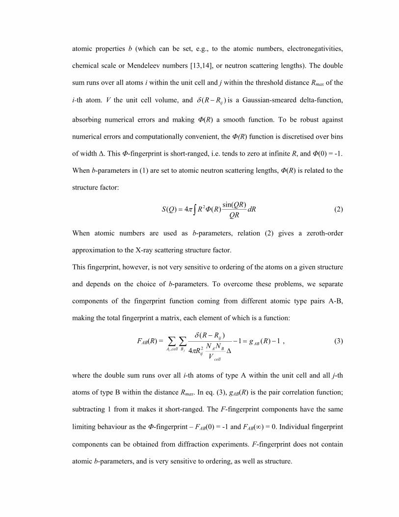
atomic properties b (which can be set, e.g., to the atomic numbers, electronegativities,

chemical scale or Mendeleev numbers [13,14], or neutron scattering lengths). The double

sum runs over all atoms i within the unit cell and j within the threshold distance Rmax of the

i-th atom. V the unit cell volume, and )( ijRR −δ is a Gaussian-smeared delta-function,

absorbing numerical errors and making Φ(R) a smooth function. To be robust against

numerical errors and computationally convenient, the Φ(R) function is discretised over bins

of width Δ. This Φ-fingerprint is short-ranged, i.e. tends to zero at infinite R, and Φ(0) = -1.

When b-parameters in (1) are set to atomic neutron scattering lengths, Φ(R) is related to the

structure factor:

∫= dRQR

QRRΦRQS )sin()(4)( 2π (2)

When atomic numbers are used as b-parameters, relation (2) gives a zeroth-order

approximation to the X-ray scattering structure factor.

This fingerprint, however, is not very sensitive to ordering of the atoms on a given structure

and depends on the choice of b-parameters. To overcome these problems, we separate

components of the fingerprint function coming from different atomic type pairs A-B,

making the total fingerprint a matrix, each element of which is a function:

FAB(R) = 1)(14

)(

, 2−=−

Δ

−∑ ∑ Rg

VNNR

RRAB

cellA B

cell

BAij

ij

i j π

δ , (3)

where the double sum runs over all i-th atoms of type A within the unit cell and all j-th

atoms of type B within the distance Rmax. In eq. (3), gAB(R) is the pair correlation function;

subtracting 1 from it makes it short-ranged. The F-fingerprint components have the same

limiting behaviour as the Φ-fingerprint – FAB(0) = -1 and FAB(∞) = 0. Individual fingerprint

components can be obtained from diffraction experiments. F-fingerprint does not contain

atomic b-parameters, and is very sensitive to ordering, as well as structure.

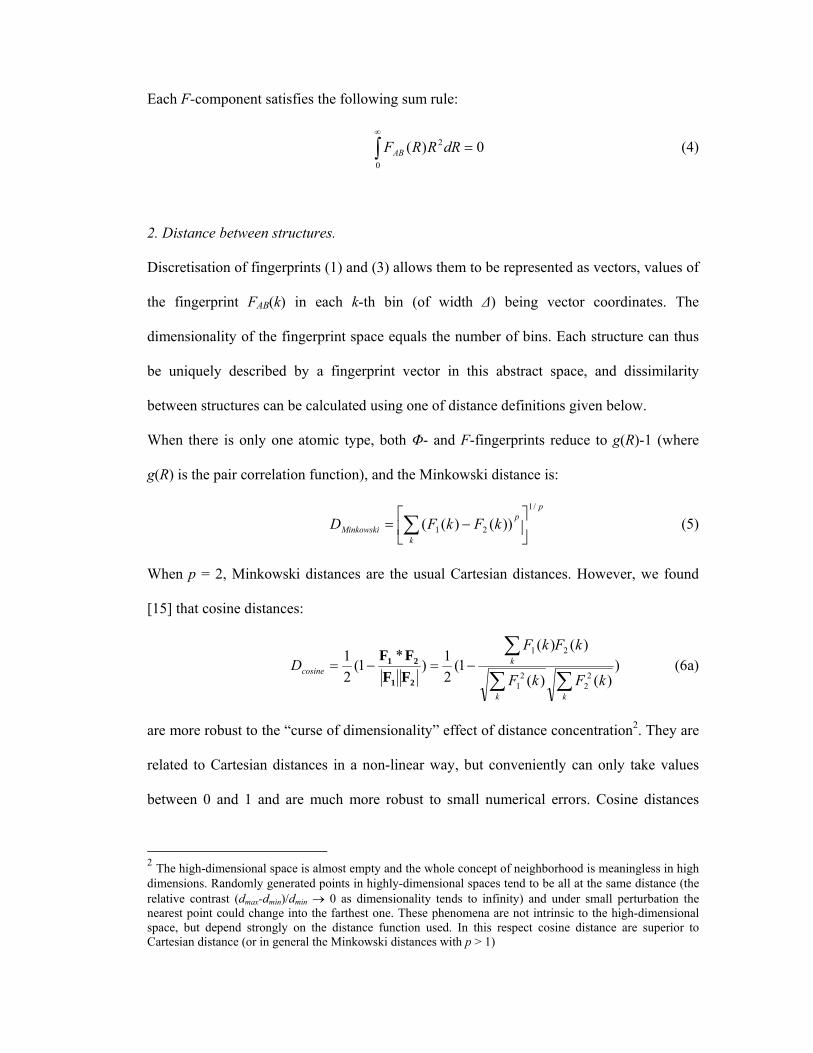
Each F-component satisfies the following sum rule:

∫∞

=0

2 0)( dRRRFAB (4)

2. Distance between structures.

Discretisation of fingerprints (1) and (3) allows them to be represented as vectors, values of

the fingerprint FAB(k) in each k-th bin (of width Δ) being vector coordinates. The

dimensionality of the fingerprint space equals the number of bins. Each structure can thus

be uniquely described by a fingerprint vector in this abstract space, and dissimilarity

between structures can be calculated using one of distance definitions given below.

When there is only one atomic type, both Φ- and F-fingerprints reduce to g(R)-1 (where

g(R) is the pair correlation function), and the Minkowski distance is:

pp

kMinkowski kFkFD

/1

21 ))()(( ⎥⎦

⎤⎢⎣

⎡−= ∑ (5)

When p = 2, Minkowski distances are the usual Cartesian distances. However, we found

[15] that cosine distances:

))()(

)()(1(

21)

*1(

21

22

21

21

∑∑

∑−=−=

kk

kcosine

kFkF

kFkFD

21

21

FFFF

(6a)

are more robust to the “curse of dimensionality” effect of distance concentration2. They are

related to Cartesian distances in a non-linear way, but conveniently can only take values

between 0 and 1 and are much more robust to small numerical errors. Cosine distances

2 The high-dimensional space is almost empty and the whole concept of neighborhood is meaningless in high dimensions. Randomly generated points in highly-dimensional spaces tend to be all at the same distance (the relative contrast (dmax-dmin)/dmin → 0 as dimensionality tends to infinity) and under small perturbation the nearest point could change into the farthest one. These phenomena are not intrinsic to the high-dimensional space, but depend strongly on the distance function used. In this respect cosine distance are superior to Cartesian distance (or in general the Minkowski distances with p > 1)

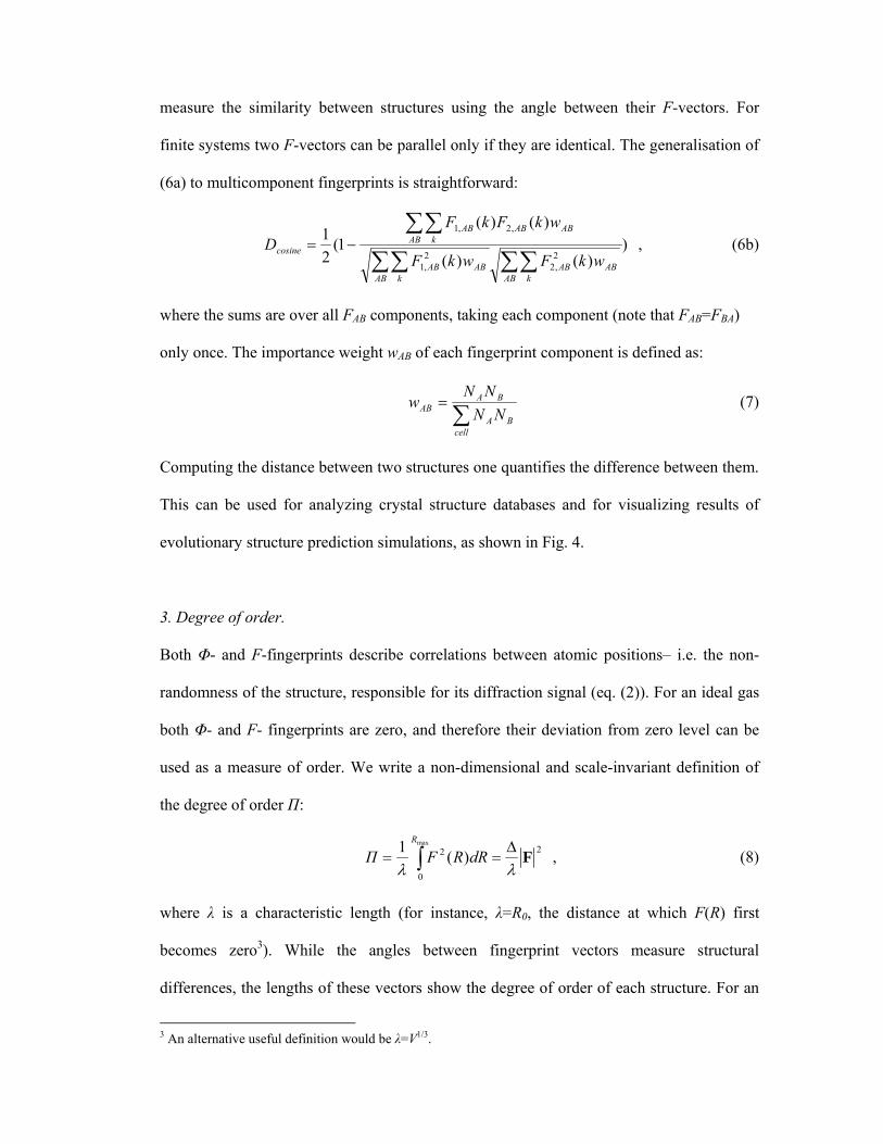
measure the similarity between structures using the angle between their F-vectors. For

finite systems two F-vectors can be parallel only if they are identical. The generalisation of

(6a) to multicomponent fingerprints is straightforward:

))()(

)()(1(

21

2,2

2,1

,2,1

∑∑∑∑

∑∑−=

AB kABAB

AB kABAB

AB kABABAB

cosinewkFwkF

wkFkFD , (6b)

where the sums are over all FAB components, taking each component (note that FAB=FBA)

only once. The importance weight wAB of each fingerprint component is defined as:

∑=

cellBA

BAAB NN

NNw (7)

Computing the distance between two structures one quantifies the difference between them.

This can be used for analyzing crystal structure databases and for visualizing results of

evolutionary structure prediction simulations, as shown in Fig. 4.

3. Degree of order.

Both Φ- and F-fingerprints describe correlations between atomic positions– i.e. the non-

randomness of the structure, responsible for its diffraction signal (eq. (2)). For an ideal gas

both Φ- and F- fingerprints are zero, and therefore their deviation from zero level can be

used as a measure of order. We write a non-dimensional and scale-invariant definition of

the degree of order Π:

2

0

2max

)(1 FλλΔ

== ∫R

dRRFΠ , (8)

where λ is a characteristic length (for instance, λ=R0, the distance at which F(R) first

becomes zero3). While the angles between fingerprint vectors measure structural

differences, the lengths of these vectors show the degree of order of each structure. For an

3 An alternative useful definition would be λ=V1/3.

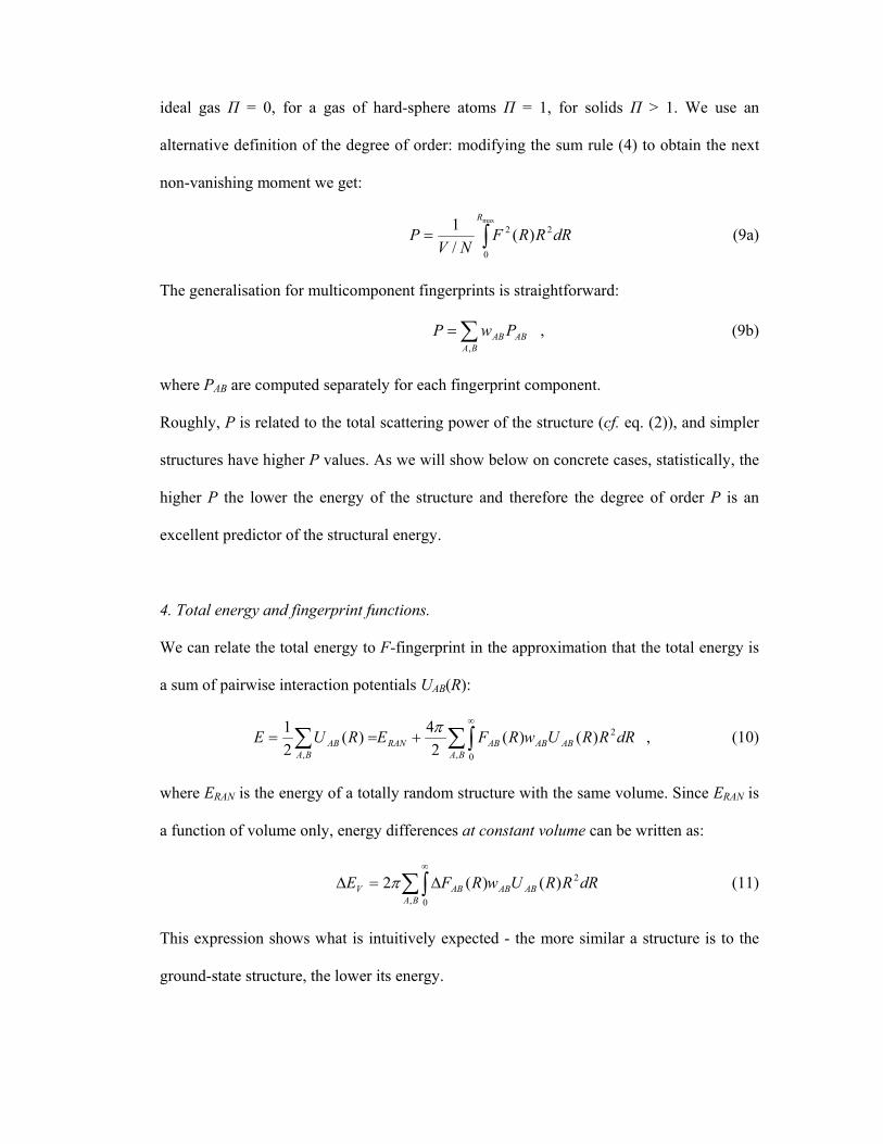
ideal gas Π = 0, for a gas of hard-sphere atoms Π = 1, for solids Π > 1. We use an

alternative definition of the degree of order: modifying the sum rule (4) to obtain the next

non-vanishing moment we get:

∫=max

0

22 )(/1 R

dRRRFNV

P (9a)

The generalisation for multicomponent fingerprints is straightforward:

∑=BA

ABAB PwP,

, (9b)

where PAB are computed separately for each fingerprint component.

Roughly, P is related to the total scattering power of the structure (cf. eq. (2)), and simpler

structures have higher P values. As we will show below on concrete cases, statistically, the

higher P the lower the energy of the structure and therefore the degree of order P is an

excellent predictor of the structural energy.

4. Total energy and fingerprint functions.

We can relate the total energy to F-fingerprint in the approximation that the total energy is

a sum of pairwise interaction potentials UAB(R):

dRRRUwRFERUE ABBA

ABABRANBA

AB2

, 0,)()(

24)(

21 ∑∫∑

∞

+==π , (10)

where ERAN is the energy of a totally random structure with the same volume. Since ERAN is

a function of volume only, energy differences at constant volume can be written as:

dRRRUwRFEBA

ABABABV2

, 0

)()(2 ∑∫∞

Δ=Δ π (11)

This expression shows what is intuitively expected - the more similar a structure is to the

ground-state structure, the lower its energy.

5. Quasi-entropy: a measure of structural diversity.

Based on our distance metric, and noting that cosine distances, just like occupation

numbers, take values between 0 and 1, we propose collective quasi-entropy:

)1ln( ijcoll DS −−= (12)

as a measure of collective diversity. Calculating Scoll for a set of structures gives a single

number measuring the diversity of that set. This is very useful for tuning global

optimization methods, where rapid decrease of quasi-entropy may indicate premature

convergence of the algorithm.

For each given structure, one may also compute its own quasi-entropy as a measure of

disorder and complexity of that structure (alternative to definitions (8) and (9)):

∑ −−=A

AAcell

Astr ji

DNN

S )1ln( , (13)

where distances ji AAD are measured between fingerprints4 of all i-th and j-th sites occupied

by chemical species A, and the total quasi-entropy is a weighted sum over all chemical

species. Standard crystallographic description gives the number of symmetrically

inequivalent atomic positions, but does not provide any measure of physical difference

between those positions – such a difference is given by eq. (13).

6. Summary of the formalism.

We have proposed two families of closely related fingerprint functions (1) and (3). Based

on these functions, we proposed a measure (6ab) of similarity (distance) between different

structures, and a new parameter (9ab) quantifying the simplicity and order of a crystal

4 For this, one needs to compute a fingerprint for each i-th atom (rather than atomic species), defined

by analogy with eq. (3) as 14

)(

2−

Δ

−= ∑

j

iB

cell

Bij

ijBA

VN

R

RRF

π

δ.

structure. Quasi-entropies (12) and (13) can be used for analysing the performance of

global optimization methods and provide another measure of structural complexity. Below

we show how these quantities can be used to map energy landscapes of solids and

rationalise them in terms of intuitive chemical concepts.

IV. Illustrations of our approach on realistic systems5.

1. Confirming the existence of energy funnels.

Chemical intuition tells us that since low-energy structures share many similarities (similar

coordination numbers, bond lengths and angles, sometimes even whole structural blocks),

they have to be clustered in the same region of parameter space. This would lead to an

overall bowl-like shape of the reduced energy surface (Fig. 1) and would have many

consequences of paramount importance. First, this would imply that low-energy structures

tend to be connected by relatively low energy barriers and short transition pathways (Bell-

Evans-Polanyi principle [24]). If there are several funnels, transitions between them are

likely to involve large activation barriers. Second, funnel-like topology of the landscape is

important for modern structure prediction methods (e.g. the evolutionary algorithm [16-19]

and all neighbourhood search methods) to be efficient.

If the funnel-like shape of the reduced energy landscape is valid, there would be a

correlation between the energy and the distance from the global minimum: the further from

the global minimum, the higher the energy. This correlation can now be easily checked and

5 In all illustrations given below, we used F-fingerprints (eq. (3)) with Rmax=15 Å, Δ = 0.05 Å, and Gaussian-smeared δ-function with σ = 0.075 Å. We use cosine distances and degree of order P (eq. 9a,b) throughout. The data analysed here include 2997 distinct local minima for GaAs (8 atoms/cell), 249 for Au8Pd4 (12 atoms/cell), 967 for MgO (32 atoms/cell), 949 for H2O (12 atoms/cell), 6977 for MgNH (12 atoms/cell), and 1949 distinct local minima for the AB2 Lennard-Jones crystal. All data were obtained in evolutionary and random sampling runs, duplicate minima were pruned using a clustering procedure described in [15]. Local optimizations for most systems were done within the generalized gradient approximation [20] (only for Au8Pd4, calculations were done within the local density approximation) using the VASP code [21]. Exceptions are MgO, for which we used the interatomic potential [22] and Lennard-Jones (see caption to Fig. 2 for the description of the potential model) systems – for both, structure relaxations and energy calculations were performed using the GULP code [23].

turns out to be excellent in many chemically simple systems – this is shown in Fig. 5 for

GaAs and in Fig. 6 for Au8Pd4.

At first surprisingly, for MgO with 32 atoms/cell the landscape turns out to be more

complex and contains three broad funnels with 6-, 5- and 4-coordinate Mg atoms,

respectively (Fig. 7a). The potential [22] used here correctly finds the ground state to have

the NaCl-type structure, and among the lowest-energy local minima we find an exciting

metastable structure with both Mg and O atoms in the fivefold coordination (Fig. 7b). This

structure was previously predicted in [26], but has not yet been identified experimentally.

Among other low-energy metastable structures are zincblende, wurtzite and their

polytypes. The ability of Mg atoms to adopt very different coordination numbers (ranging

from 4 to 8) in oxides and silicates is well known to mineralogists, and is the key to the

multi-funnel structure of the landscape. Fig. 7a shows that the funnels almost “touch” each

other and there are low-energy structures close to the boundaries between funnels. This

means that there may be relatively low-energy transition pathways between the funnels,

and the landscape can be considered intermediate between single-funnel and multi-funnel

types. The non-monotonic energy-distance plot reflects the complicated topology of the

landscape very clearly (Fig. 7c).

An extremely clear depiction of a multi-funnel energy landscape is provided by H2O with

12 atoms/cell. This landscape contains (at least) three clearly separated and chemically

distinct funnels (Fig. 8). These funnels have very different energies – structures in the

deepest funnel consist of H2O molecules, whereas structures belonging to the two higher-

energy funnels contain various mixtures of molecular groups (H2O, H2, O2, OH-, many

structures contain H2O2 and some H2O3 molecules). In many structures we find OH- ions,

which is at variance with previous calculations [27] where these ions were not seen at all.

The energy-distance correlation is clearly seen across the landscape and, of course, within

each funnel (Fig. 8b).

Among the systems we explored, the most complex landscapes are found for MgNH and

AB2 Lennard-Jones crystal with the potential described in caption to Fig. 2. Both systems,

though small (12 atoms/cell), possess remarkable complexity with multiple degeneracies.

For instance, for MgNH we found 25 structures with energies less than 2.5 meV/atom

above the ground state. Most of these structures contain NH2- groups, though some have

(NH2)- and N3- ions - low energies of the latter structures suggest (in agreement with

experiment) that MgNH is only marginally stable with respect to decomposition into

Mg3N2+Mg(NH2)2. Generally, the existence of funnels with energies close to the ground

state indicates that the system is close either to a phase transition or to decomposition. The

2D-map of the landscape and the energy-distance correlation plot for MgNH (Fig. 9a) show

low-energy funnels, some of which show very obvious structural differences. One of the

funnels consists entirely of layered structures, whereas in another funnel all structures

contain either parallel or antiparallel NH- groups. Finally, we note the gap in the energy

distribution, related to the dissociation of molecular ions – the higher-energy structures

contain atomic/ionic hydrogen, the formation of which requires breaking N-H bonds.

For the AB2 Lennard-Jones crystal the energy-distance plot (Fig. 9b) has several flat

regions with nearly constant energies, a feature characteristic of strong degeneracy. We

will see in the next section that several families of structures exist here, and within each

family the energy is nearly constant. The degeneracies originate from the short-rangedness

of interatomic interactions, where the length scale of typical geometric features (in this

case, interplanar distances) is longer than the range of interatomic interactions, and in the

competition between different interactions (in this model, A-A, B-B and A-B interactions

have the same strength and thus compete). Such degeneracies and complex energy

landscapes (probably less extreme than the case presented in Fig. 9b) may be expected in

systems forming quasicrystals and incommensurate phases, as well as systems unstable (as

the AB2 crystal here) or nearly unstable (as MgNH) agaist decomposition.

2. Does nature prefer simple structures?

Pauling’s fifth rule [28] states that “the number of essentially different kinds of constituents

in a crystal tends to be small” – in other words, structures tend to be simple. Some have

accepted this rule, some criticized it. Our approach enables its systematic analysis from the

viewpoint of structural energies. If Pauling’s rule is valid, one should see a clear correlation

between the energy and degree of order. Finding cases where the correlation breaks down

would indicate the limits of its applicability.

A vast majority of cases that we analysed shows an excellent correlation between the

energy and the degree of order. This correlation is equally good for single- and multi-

funneled landscapes; in other words, it is more fundamental. For GaAs, MgO and H2O

ground states are the most ordered structures among the multitude of structures that we

generated. For Au8Pd4 the ground state is among very few most ordered structures, and

even for heavily frustrated systems, such as MgNH and AB2 Lennard-Jones crystal, the

ground states still belong to a small number of most ordered structures. Fig. 10 shows such

correlation plots for MgO, Au8Pd4, H2O and Lennard-Jones AB2 crystal.

Furthermore, we see that all chemically interesting structures are on the high-order side of

the correlation plots. We illustrate this point for MgO (Fig. 10a), where a number of

interesting and even unexpected low-energy ordered structures were found with the help of

such a correlation plot. For AB2 Lennard-Jones crystal, we again see families of structures

with nearly identical energies. The two most ordered families include a family of defective

NaCl-type structures (cubic close-packings of the B atoms, with a half of octahedral voids

occupies by the A atoms – the well-known CdCl2 structure type also belongs to this family)

and a family of layered structures, where the B atoms form a defective hexagonal close

packing, interrupted by layers of the A atoms in the trigonal prismatic coordination (Fig.

11). It is the latter family that contains several degenerate ground-state structures. The A-

layers are topologically identical to the graphene sheet, and there is a striking structural

similarity between the ground states of the AB2 Lennard-Jones crystal and Al-C alloys

[29]. Another similarity is that both Al-C alloys and the AB2 Lennard-Jones crystal are

unstable to decomposition into pure elements.

Recently, Hart [30] found that for the special case of ordering in alloys the simplest

ordering schemes have the highest probability of occurring6. Here we have generalised this

conclusion to all structures (i.e. beyond the special case of ordering in alloys) and

confirmed it by analysing structural energies. We can conclude that: The ground state

normally adopts one of the simplest structures compatible with the chemistry of the

compound. Such structures tend to have lower energies. This rule is nothing else than an

energetics-based reformulation of Pauling’s fifth rule. The main limitation of this rule is the

presence of competing interactions, as in the case of AB2 Lennard-Jones crystal (Fig. 10 e).

Structural quasi-entropy Sstr, which is zero when each atomic species occupies only one

Wyckoff orbit and increases as the physical difference between the occupied sites

increases, is another and perhaps even more direct measure of structural simplicity. It more

directly relates to the original [28] formulation of Pauling’s 5th rule. Unlike the degree of

order, Sstr does not depend critically on the smoothing function δ(R-Rij) in the fingerprint

definition (eqs. 1,3) and its absolute (not only relative) values are meaningful. For all cases

investigated here, we found an excellent correlation between the energy and quasi-entropy

6 To quantify the simplicity of an alloy structure, Hart [30] introduced an index measuring the non-randomness of the distribution of atoms over sites. His index is valid only for the case of ordering in alloys. Our degree of order (eq. 9a,b) provides a universal criterion, equally valid for ordering in alloys of a given structure, as well as for the comparison of completely different structures.

Sstr – this is shown in Fig. 12 for MgO (32 atoms/cell) and MgNH (12 atoms/cell). Like

with the degree of order P, the correlation is worst for the AB2 Lennard-Jones crystal, the

reason being its instability to decomposition that leads to long-period layered structures

that contain quite diverse atomic sites. The same can be expected for other complex and

frustrated systems. A good example of which is the recently discovered [31] high-pressure

stable phase of boron, the structure of which contains atomic sites that are so different that

there is charge transfer between them [31] and the structure possesses large Sstr=0.18.

which formulates an intuitively reasonable expectation that in stable structures atoms

occupy. Our conclusion is that: In the ground state and low-energy structures, atoms of

each species tend to occupy similar crystallographic sites.

The degree of order P and structural quasi-entropy Sstr are not the only possible measures

of structural simplicity. One alternative is the set of orientational bond order parameters Qn

proposed by Steinhardt [8]. These parameters successfully differentiate between liquid-like

and crystal-like configurations and could be expected to be good predictors of the energy.

However, for all systems examined here (even as simple as MgO) the correlation of these

parameters with the energy is either very weak or non-existent – Fig. 13 shows this for the

Q6 parameter (we also checked for Q4, as well as W4 and W6 parameters [3132], and arrived

at the same conclusion). Thus, the degree of order P and structural quasi-entropy Sstr are

strong predictors of the energy, whereas the orientational bond order parameters Qn and Wn

are not.

Conclusions.

We have introduced a number of powerful tools to investigate structures and energy

landscapes of crystalline systems. These tools can be used for rationalising structural and

thermodynamic information on solids.

The basic function, from which all others are derived, is the fingerprint (eq. 3), which can

be represented as a vector in an abstract multidimensional space. The possibility of

computing a well-defined index of similarity (“distance”) between two crystal structures is

valuable for many purposes – as two examples, we mention monitoring of the progress of

structure prediction simulations [16] and the emerging field of crystallographic genomics

[33], where such analysis is central for the rationalisation of large databases of crystal

structures.

Typical dimensionalities of fingerprint vector spaces for cases studied here, 102-103, are

clearly redundant compared to the true dimensionality d = 3N + 3 (N is the number of

atoms in the unit cell). However, even d overestimates the true dimensionality of the

landscape, because it ignores short-range order that leads to certain constraints κ in relative

positions of the atoms. The actual intrinsic dimensionality:

d* = 3N + 3 – κ (14)

is generally a non-integer number and can be computed from the distance distribution.

Using the Grassberger-Procaccia algorithm in the modification [34], we obtain d* = 10.85

(d = 39) for Au8Pd4, d* = 32.5 (d = 39) for MgNH and d* = 11.6 (d = 99) for MgO. The

intrinsic dimensionality gives the minimum number of dimensions sufficient for mapping

the data exactly, but approximate mappings can be done in lower dimensions.

By allowing direct mapping of energy landscapes in any number of dimensions – from 1

(energy-distance plots extensively used here) to 2 (landscape “maps” also presented here)

to as many dimensions as needed, such analysis leads to a new level of chemical insight.

Based on the fingerprint function, we introduced two indices of structural simplicity, the

degree of order P (eq. 9ab) and structural quasi-entropy Sstr (eq. 13), which enabled us to

directly verify the well-known Pauling’s fifth rule (the parsimony rule): statistically,

simpler structures tend to have lower energies. Parameters P and Sstr are powerful tools for

analyzing results of crystal structure prediction simulations (see [15]) and crystal structure

databases. This analysis can be brought further: for instance, energy-order correlations for

order components PAB (eq. 9b) may indicate the dominant structure-forming interactions

and causes of geometric frustrations.

The tools developed here are helpful in monitoring structure prediction simulations, as

shown in Fig. 14. Furthermore, these tools, as well as improved understanding of energy

landscapes, can be (and already have been [35]) used to improve performance of the

existing global optimization methods for crystal structure prediction.

The same analysis can be done for the physical properties of crystals, leading to the

discovery of interesting structure-property relations. For many properties we also expect to

observe funnel-shapes landscapes, which would indicate types of structures that are of

particular interest. Many properties (e.g. the electrical conductivity) are expected to be well

correlated with the degree of order P and structural quasi-entropy Sstr. The analysis

presented here can thus provide the general link between the structure, properties and

stability of solids.

Acknowledgments. The formalism discussed here has been implemented by M.V. in the

STM4 toolkit, freely available toolkit, freely available at:

http://www.cscs.ch/~mvalle/STM4; fingerprint libraries can be found at:

http://trac.cscs.ch/crystalfp. We greatly appreciate discussions with A.O. Lyakhov. This

work was supported by Swiss National Science Foundation (grants 200021-111847/1 and

200021-116219).

References:

1. Stillinger F.H. (1995). A topographic view of supercooled liquids and glass formation. Science. 267,

1935-1939.

2. Wales D.J., Miller M.A., Walsh T.R. (1998). Archetypal energy landscapes. Nature 394, 758-760.

3. Angelani L., Ruocco G., Sampoli M. (2003). General features of the energy landscape in Lennard-Jones-

like model liquids. J. Chem. Phys. 119, 2120-2127.

4. Shah P., Chakravarty C. (2002). Potential-energy landscapes of simple solids. Phys. Rev. Lett. 88,

255501.

5. Büchner S., Heuer A. (1999). Potential energy landscape of a model glass former: Thermodynamics,

anharmonicities, and finite size effects. Phys. Rev. E60, 6507-6518.

6. Heuer A. (1997). Properties of a glass-forming system as derived from its potential energy landscape.

Phys. Rev. Lett. 78, 4051-4054.

7. Becker O.M., Karplus M. (1997). The topology of multidimensional potential energy surfaces: theory

and application to peptide structure and kinetics. J Chem. Phys. 106, 1495-1517.

8. Steinhardt P.J., Nelson D.R., Ronchetti M. (1983) Bond-orientational order in liquids and glasses. Phys.

Rev. B28, 784-805.

9. Willighagen E.L., Wehrens R., Verwer P., de Gelder R., and Buydens L.M.C. (2005). Method for the

computational comparison of crystal structures. Acta Crystallogr., B61, 29–36.

10. de Gelder R. (2006). Quantifying the similarity of crystal structures. IUCr CompComm Newsletter, 7,

59–69.

11. Doye J.P.K. (2002). Network topology of a potential energy landscape: a static scale-free network. Phys.

Rev. Lett. 88, 238701.

12. Doye J.P.K., Miller M.A., Wales D.J. (1999). The double-funnel energy landscape of the 38-atom

Lennard-Jones cluster. J. Chem. Phys. 110, 6896-6906.

13. Pettifor D.G. (1984). A chemical scale for crystal structure maps. Solid State Commun. 51, 31-34.

14. Pettifor D.G. (1986). The structures of binary compounds: I. Phenomenological structure maps. J. Phys.

C19, 285-313.

15. Valle M., Oganov A.R. (2008). Crystal structure classifier for an evolutionary algorithm structure

predictor. IEEE Symposium on Visual Analytics Science and Technology (October 21 - 23, Columbus,

Ohio, USA), pp. 11- 18.

16. Oganov A.R., Ma Y., Glass C.W., Valle M. (2007). Evolutionary crystal structure prediction: overview

of the USPEX method and some of its applications. Psi-k Newsletter, number 84, Highlight of the

Month, 142-171.

17. Oganov A.R., Glass C.W., Ono S. (2006). High-pressure phases of CaCO3: crystal structure prediction

and experiment. Earth Planet. Sci. Lett. 241, 95-103.

18. Oganov A.R., Glass C.W. (2006). Crystal structure prediction using ab initio evolutionary techniques:

principles and applications. J. Chem. Phys. 124, art. 244704.

19. Glass C.W., Oganov A.R., Hansen N. (2006). USPEX – evolutionary crystal structure prediction. Comp.

Phys. Comm. 175, 713-720.

20. Perdew J.P., Burke K., Ernzerhof M. (1996). Generalized gradient approximation made simple. Phys.

Rev. Lett. 77, 3865-3868.

21. Kresse G. & Furthmüller J. (1996). Efficiency of ab initio total-energy caclulations for metals and

semiconductors using a plane-wave basis set. Comp. Mater. Sci. 6, 15-50.

22. Lewis G.V. & Catlow C.R.A. (1985). Potential models for ionic oxides. J. Phys. C.: Solid State Phys. 18,

1149-1161.

23. Gale J.D. (2005). GULP: Capabilities and prospects. Z. Krist. 220, 552-554.

24. Roy S., Goedecker S., Hellmann V. (2008). Bell-Evans-Polanyi principle for molecular dynamics

trajectories and its implications for global optimization. Phys. Rev. E77, 056707.

25. Oganov A.R., Ma Y., Glass C.W., Valle M. (2007). Evolutionary crystal structure prediction: overview

of the USPEX method and some of its applications. Psi-k Newsletter, number 84, Highlight of the

Month, 142-171.

26. Schon J.C., Jansen M. (1996). First step towards planning of syntheses in solid-state chemistry:

determination of promising structure candidates by global optimisation. Angew. Chem. – Int. Ed. 35,

1287-1304.

27. Pickard C.J., Needs R.J. (2007). When is H2O not water? J. Chem. Phys. 127, 244503.

28. Pauling L. (1928). The principles determining the structure of complex ionic crystals. J. Am. Chem. Soc.

51, 1010-1026.

29. Oganov A.R., Glass C.W. (2008). Evolutionary crystal structure prediction as a tool in materials design.

J. Phys.: Cond. Mattter 20, art. 064210.

30. Hart G.L.W. (2007). Where are Nature's missing structures? Nature Materials 6, 941-945.

31. Oganov A.R., Chen J., Gatti C., Ma Y.-M., Yu T., Liu Z., Glass C.W., Ma Y.-Z., Kurakevich O.O.,

Solozhenko V.L. (2009). Ionic high-pressure form of elemental boron. Nature, in press.

32. van Duijneveldt J.S., Frenkel D. (1992). Computer simulation study of free energy barriers in crystal

nucleation. J. Chem. Phys. 96, 4655-4668.

33. Parkin A., Barr G., Dong W., Gilmore C.J., Jayatilaka D., MCKinnon J.J., Spackman M.A., Wilson C.C.

(2007). Comparing entire crystal structures: structural genetic fingerprinting. CrystEngComm 9, 648-652.

34. Camastra F., Vinciarelli A. (2001). Intrinsic dimension estimation of data: an approach based on

Grassberger-Procaccia’s algorithm. Neural Proc. Lett. 14, 27-34.

35. Lyakhov A.O., Oganov A.R., Valle M. (2009). How to predict large and complex crystal structures. In

prep.

FIGURE CAPTIONS:

Fig. 1. Conceptual depiction of an energy landscape (solid line) and reduced energy

landscape (filled squares connected by dashed lines). From [16].

Fig. 2. DOS of energy minima for (a) GaAs with 8 atoms/cell and (b) binary Lennard-

Jones crystal AB2 for several system sizes. Energies are shown relative to the ground

state. Data were obtained by locally optimising random structures, without pruning

identical structures. In (a), 3000 random structures were sampled, while in (b) we typically

sampled 5000 random structures at each system size. Calculation (a) was done using the

generalized gradient approximation [20] of density functional theory. In (b), for each

atomic pair the Lennard-Jones potential was written as ⎥⎦

⎤⎢⎣

⎡−= 6min,12min, )(2)(

RR

RR

U ijijijij ε ,

where Rmin,ij is the distance at which the potential reaches minimum, and ε is the depth of

the minimum). For all pairs we used the same ε, but different ideal lengths:

Rmin,BB=1.5Rmin,AB=2Rmin,AA. Competition between these simple spherically-symmetric

interactions leads to very complex energy landscapes and non-trivial ground states.

Fig. 3. F-fingerprint of the ground-state structure of Au8Pd4 (12 atoms/cell) found in

[16].

Fig. 4. Similarity matrix (dimensions 630x630) for an evolutionary structure

prediction simulation for Au8Pd4 (with 12 atoms/cell) at 1 atm. Each (N,M) pixel shows

the distance between the N-th and M-th structures. Note the increase of similarity between

the structures towards the end of the simulation – this is a consequence of “learning” in

evolutionary simulations. This matrix is by construction symmetric with respect to its

diagonal, and all diagonal (N,N) elements are zero (structure N is identical to itself).

Fig. 5. Energy-distance correlation for 2997 distinct local minima of GaAs (8

atoms/cell). The minima were found in several ab initio evolutionary and random

sampling simulations. Energy differences (per unit cell) and distances in this and all

subsequent graphs are relative to the ground state.

Fig. 6. Energy-distance correlation based on 249 distinct local minima of Au8Pd4

obtained in an ab initio evolutionary run [24]. Most structures are different decorations

of f.c.c. or h.c.p. structures.

Fig. 7. Energy landscape for MgO with 32 atoms/cell. (a) 2D-mapping of the landscape,

where each point represents a structure and distances between points on the graph are

maximally close to the distances between the corresponding fingerprints7. Darker points

indicate lower-energy structures. (b) Metastable structure of MgO with 5-coordinate Mg

and O atoms in the trigonal bipyramidal coordination. It has the space group P63/mmc, cell

parameters a=b=3.46 Å and c=4.18 Å, and atomic positions Mg (1/3, 2/3, 3/4) and O (2/3,

1/3, 3/4). (c) Energy-distance correlation.

Fig. 8. Energy landscape of H2O with 12 atoms/cell. (a) 2D-map of the landscape with

darker points indicating lower-energy structures. (b) Energy-distance correlation. The inset

shows only the 580 structures based on H2O molecules.

7 Of course, such mapping with reduced dimensionality cannot fully preserve distances (for the same reason, 2D-maps of the world show distorted distances). However, the topology of the landscape is correctly reproduced.

Fig. 9. Complex energy landscapes : (a) MgNH (12 atoms/cell) and (b) AB2 Lennard-

Jones crystal (12 atoms/cell).

Fig. 10. Energy-order correlation plots. (a) MgO (32 atoms/cell), (b) Au8Pd4 (12

atoms/cell), (c) H2O (12 atoms/cell), with inset showing only the 580 structures containing

only H2O molecules, (d) MgNH (12 atoms/cell) and (2) AB2 Lennard-Jones crystal (12

atoms/cell). Large red squares indicate the ground state.

Fig. 11. Families of nearly degenerate structures for AB2 Lennard-Jones crystal (12

atoms/cell). (a-c) ground states with layers of the A atoms in the trigonal prismatic

coordination, (d,e) defective NaCl-type structures. Structure (a) is the lowest-energy

structure we found.

Fig. 12. Energy – structural quasi-entropy Sstr correlation plots. (a) MgO (32

atoms/cell), (b) MgNH (12 atoms/cell). Note a clear energetic preference for simple

structures (those with lowest quasi-entropy).

Fig. 13. Energy-Q6 correlation plots. (a) MgO (32 atoms/cell), (b) AB2 Lennard-Jones

crystal (12 atoms/cell). It is obvious that, unlike the degree of order P (eq. 9ab) or

structural quasi-entropy (eq. 13), the orientational bond order parameter Q6 is not a good

predictor of energy.

Fig. 14. Progress of an evolutionary structure prediction simulation of the AB2

Lennard-Jones crystal (12 atoms/cell). Despite complexities of the energy landscape of

this system (the ground state was found only once after relaxing 5000 random structures),

the evolutionary algorithm USPEX [1619] finds the ground state after only 110 structure

relaxations. The initial population consisted of 50 random structures, and each subsequent

generation consisted of 10 best old non-identical structures and 10 new structures produced

from them using the variation operators described in [1619]. In each generation the

collective quasi-entropy Scoll was computed for a set of structures that were used for

producing the next generation. Scoll should not decrease too fast, and when it becomes

sufficiently small, the simulation can be terminated. Inset shows the lowest energy as a

function of generation number.

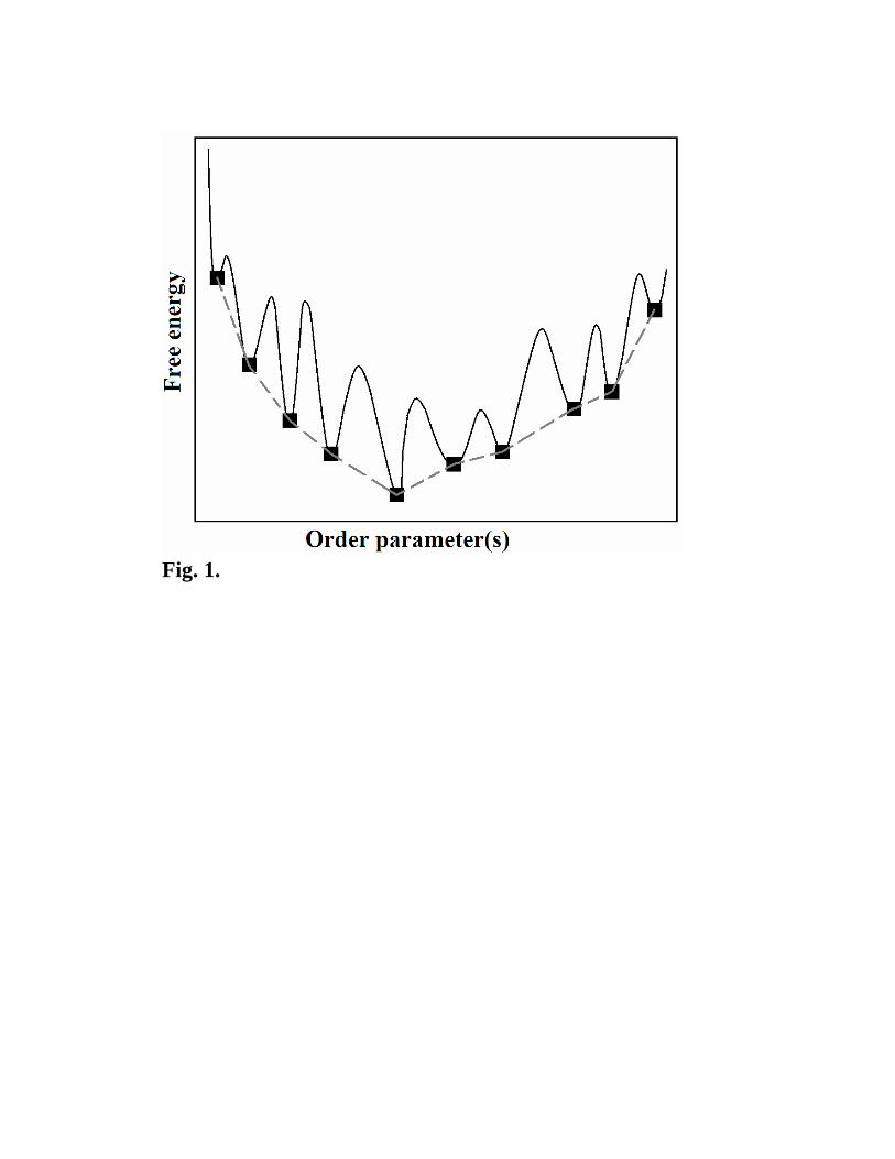
Fig. 1.

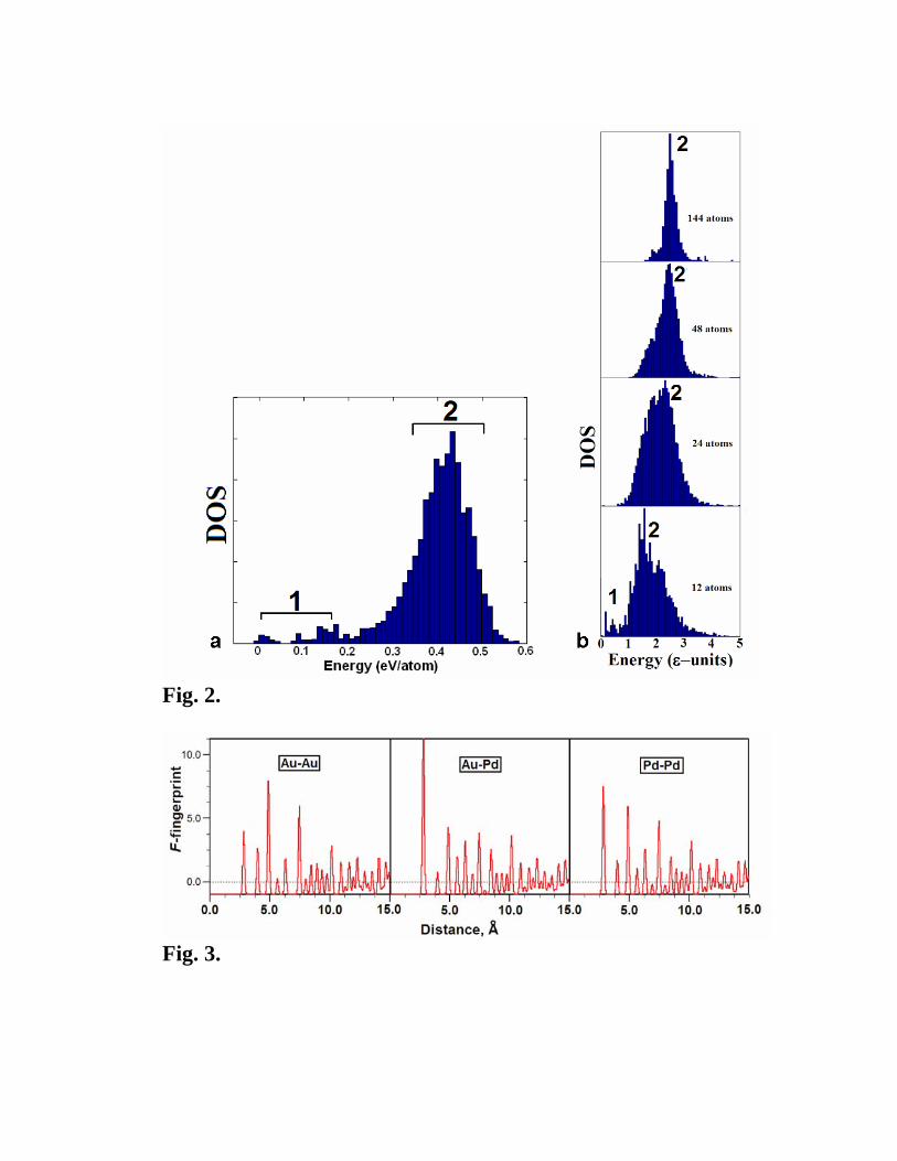
Fig. 2.

Fig. 3.

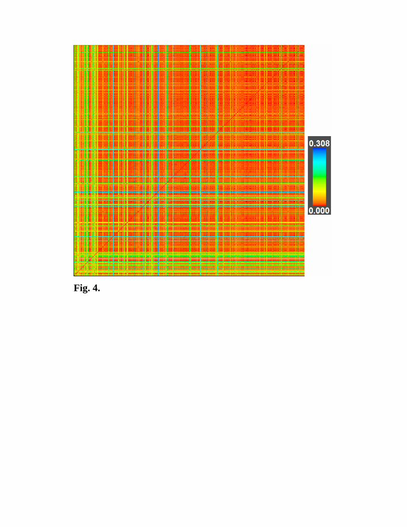
Fig. 4.

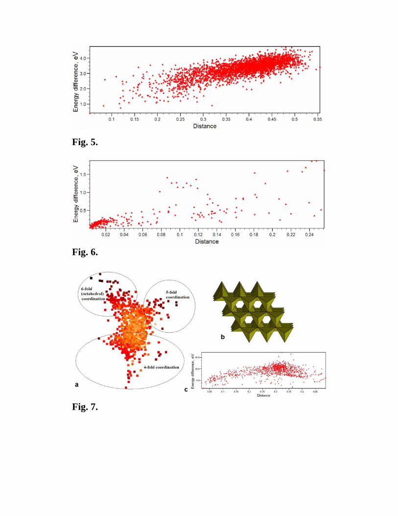
Fig. 5.

Fig. 6.

Fig. 7.

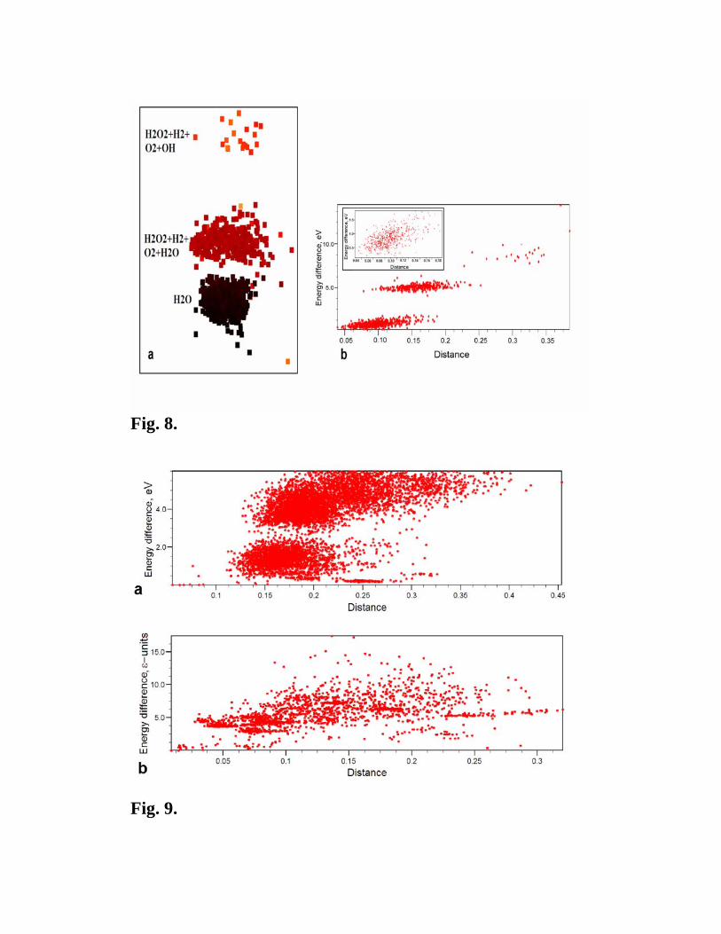
Fig. 8.

Fig. 9.

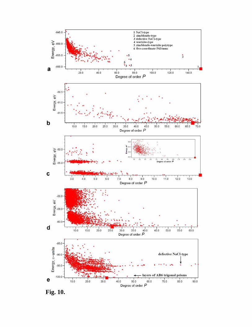
Fig. 10.

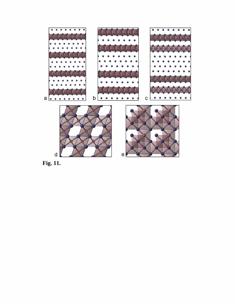
Fig. 11.

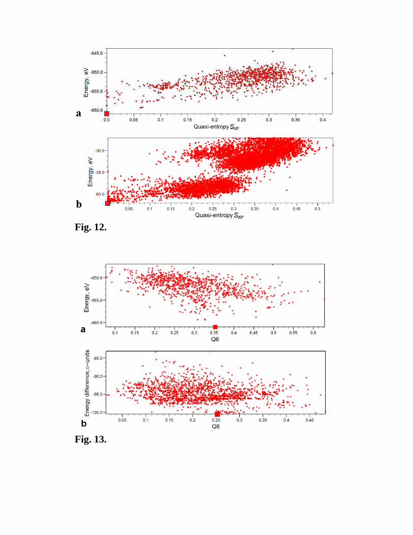
Fig. 12.

Fig. 13.

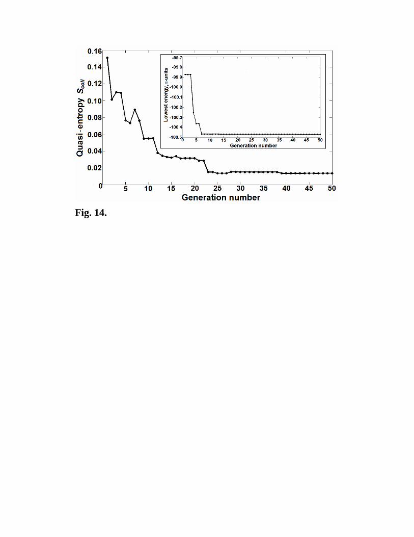
Fig. 14.