further development of a centrifugal solids
TRANSCRIPT

FURTHER DEVELOPMENT OF A CENTRIFUGAL SOLIDS SEPARATOR PROTOTYPE
T H E S I S – D E G R E E P R O G R A M I N E N V I R O N M E N T A L T E C H N O L O G Y SAVONIA UNIVERSITY OF APPLIED SCIENCES
Author:
Priscila Gandhi Estrada Reynoso
SAVONIA UNIVERSITY OF APPLIED SCIENCES THESIS Abstract
Field of Study Technology, Communication and Transport
Degree Program Degree Program in Environmental Technology Author Priscila Gandhi Estrada Reynoso
Title of Thesis
Further Development of a Centrifugal Solids Separator Prototype
Date 9 May 2016 Pages/Appendices 78 / 2
Supervisors Mr. Pasi Pajula, Principal Lecturer and Mr. Teemu Räsänen, Lecturer
Client Organization /Partners SansOx Ltd
Abstract This thesis was made for SansOx Ltd, part of the Finnish Cleantech cluster of companies, whose innovative ideas
in the water treatment area have been awarded the WssTP Water Innovation SME Award for two consecutive
years. The purpose of the thesis was to make a deeper theoretical research of the physical aspects related to solids
separation in one of SansOx’s innovations, a centrifugal solids separation device. Based on this research, it was
aimed to make a review of the previous tests of the pilot-scale prototypes of the device as well as to develop a
plan that would be the base for testing a prototype in a laboratory-scale.
The theory of solids separation in the device is strongly linked to hydraulics and particle settling, so the theoretical
research was divided into three main subjects: physics and hydraulics, particle separation, and solid separation
methods. Some basic principles of physics, such as vectors and forces, are the base for explaining the hydraulics
related to fluid flow through pipes as well as for explaining the basic theory of particle settling. Solids separation
methods were studied for a comparison between the commonly used methods in water treatment and SansOx’s
device. With the information of the theoretical research, a review of the conditions of the previous tests of the
prototype could be made, as well as finding a cause for the results obtained in the tests. Lastly, the same calcula-
tions were used to develop the sizing and testing plan of a laboratory-scale prototype.
The results of the calculations showed that the main challenge in the previous testing of the prototypes was to
achieve a discharge that would be high enough for separation. The parameters and calculations related to the
solids separation were gathered into one single Excel workbook that would serve as a tool for designing a prototype
depending on the characteristics of the solution to be treated. Finally, with this tool, a plan for the laboratory-scale
prototype was developed.
Keywords Water treatment, hydraulics, settling, solids removal, centrifugation
SAVONIA-AMMATTIKORKEAKOULU OPINNÄYTETYÖ Tiivistelmä
Koulutusala Tekniikan ja liikenteen ala Koulutusohjelma Ympäristöteknologian koulutusohjelma
Työn tekijä Priscila Gandhi Estrada Reynoso
Työn nimi
Keskipakovoimaan perustuvan kiintoaineenerotuslaitteen prototyypin jatkokehitys
Päiväys 9.5.2016 Sivumäärä/Liitteet 78 / 2
Ohjaajat
Yliopettaja Pasi Pajula ja lehtori Teemu Räsänen
Toimeksiantaja/Yhteistyökumppani
SansOx Oy
Tiivistelmä Opinnäytetyön tilaajana oli SansOx Oy, joka on yksi Suomen Cleantech -yrityksistä ja jonka innovatiiviset ideat on
palkittu WssTP Water Innovation SME Award -palkinnolla kahtena peräkkäisenä vuonna. Opinnäytetyön tavoitteena
oli tehdä teoriatarkastelu fysikaalisista ilmiöistä, jotka liittyvät SansOx:n kehittämään innovatiiviseen kiintoai-
neenerotusmenetelmään. Tarkasteltava menetelmä perustuu keskipakovoiman hyödyntämiseen, kun erotetaan
kiintoainetta nestefaasista. Tehdyn teoriatarkastelun perusteella on mahdollista arvioida aikaisempien laitteistopro-
totyyppien toimintaa ja testauksen tuloksia. Teoriatarkastelu luo samalla perustan laitteiston laboratoriomittakaa-
vaan kehitettävän version suunnittelutyöhön ja testaukseen.
Kiintoaineenerotuksen teoria liittyy vahvasti hydrauliikkaan ja partikkelin laskeutukseen, joten teoriatarkastelu oli
jaettu kolmeen pääaiheeseen: fysiikka ja hydrauliikka, partikkelin erotus sekä kiintoaineenerotusmenetelmät. Fy-
siikan peruskäsitteet, kuten vektorit ja voimat, täydentävät putkessa virtaavan nesteiden hydrauliikan sekä partik-
kelin laskeutuksen teoriaa. Muita kiintoaineenerotusmenetelmiä tarkasteltiin, jotta kehitettyä laitteistoa voitiin ver-
rata yleisesti vesien käsittelyssä käytettyihin menetelmiin. Teoriatarkastelun tietojen perusteella, voitiin arvioida
aikaisempien prototyyppien toimintaedellytyksiä ja kyettiin löytämään selittäviä tekijöitä kenttäkokeissa saatuihin
tuloksiin. Lopuksi, samoja laskelmia käyttäen pystyttiin kehittämään laitteiston seuraavan laboratoriomittakaavan
prototyypin konstruktio ja testaussuunnitelma.
Laskelmien tulokset osoittivat, että laitteiston aikaisempien prototyyppien kenttäkokeiden keskeisenä haasteena oli
riittävän suuren virtaaman aikaansaaminen laitteistoon. Kiintoaineenerotukseen liittyvät laskelmat ja niiden para-
metrit koottiin Excel-työkirjaan, joka voidaan hyödyntää jatkossa suunniteltaessa uusia laitteita erilaisiin kohteisiin.
Lopuksi, saman Excel-työkirjan avulla laadittiin suunnitelma laitteiston laboratoriomittakaavan prototyypin kon-
struktioksi.
Avainsanat Vedenkäsittely, hydrauliikka, laskeutus, kiintoaineenerotus, keskipakovoima
4 (78)
CONTENTS
1 INTRODUCTION .................................................................................................................. 6
2 PHYSICS AND HYDRAULICS ................................................................................................. 8
Vectors .................................................................................................................................. 8
2.1.1 Vector addition, subtraction and multiplication by a scalar ............................................... 8
2.1.2 Coordinate representation .......................................................................................... 10
Force ................................................................................................................................... 10
2.2.1 Gravitational force ..................................................................................................... 11
2.2.2 Centrifugal force ........................................................................................................ 12
2.2.3 Drag force ................................................................................................................ 12
Properties of fluids ................................................................................................................ 13
2.3.1 Density ..................................................................................................................... 13
2.3.2 Pressure ................................................................................................................... 14
2.3.3 Viscosity ................................................................................................................... 14
Pipe flow .............................................................................................................................. 16
2.4.1 Reynold’s number ...................................................................................................... 18
2.4.2 Continuity equation ................................................................................................... 19
2.4.3 Bernoulli equation ..................................................................................................... 19
2.4.4 Head loss .................................................................................................................. 21
2.4.5 Pumps ...................................................................................................................... 26
3 PARTICLE SEPARATION ..................................................................................................... 30
Particle characteristics ........................................................................................................... 30
3.1.1 Particle shape ........................................................................................................... 30
3.1.2 Particle size ............................................................................................................... 31
3.1.3 Particle charge .......................................................................................................... 31
3.1.4 Particle density .......................................................................................................... 32
3.1.5 Particle destabilization ................................................................................................ 33
Particle settling ..................................................................................................................... 34
3.2.1 Discrete settling ........................................................................................................ 34
3.2.2 Flocculent settling ...................................................................................................... 35
3.2.3 Hindered settling ....................................................................................................... 36
3.2.4 Compression settling .................................................................................................. 37
5 (78)
4 SOLID SEPARATION METHODS .......................................................................................... 38
Screening ............................................................................................................................. 38
Sedimentation ...................................................................................................................... 38
Flotation ............................................................................................................................... 40
Filtration .............................................................................................................................. 41
Centrifugation ....................................................................................................................... 43
4.4.1 Centrifuges ............................................................................................................... 43
4.4.2 Hydrocyclones ........................................................................................................... 45
5 SAOXFUGE PROTOTYPES ................................................................................................... 47
6 REVIEW OF THE PREVIOUS TESTS OF THE PROTOTYPES .................................................... 53
7 LABORATORY-SCALE PROTOTYPE DEVELOPMENT ............................................................... 59
8 CONCLUSIONS .................................................................................................................. 67
REFERENCES .......................................................................................................................... 69
APPENDIX 1. SAOXFUGE SPIRAL PROTOTYPE .......................................................................... 72
APPENDIX 2. EXCEL WORKBOOK TOOL ................................................................................... 73
6 (78)
1 INTRODUCTION
“Water is a limited natural resource and a public good fundamental for life and health. The
human right to water is indispensable for leading a life in human dignity. It is a prerequisite
for the realization of other human rights.”
United Nations Committee on Economic, Social, and Cultural Rights (2002)
Water, as it is found in nature, rarely fulfills the quality requirements set for human use without
previous treatment. Many human activities, from personal and domestic activities to industrial activi-
ties, can affect the quality and quantity of water. The purpose of water treatment is to provide safe
water to human use, while taking into consideration aesthetical and technical issues. Aesthetical as-
pects include color, smell, and flavor, among others, while technical aspects are related to corrosion
and damage of pipes and fittings. (RIL I 2003, 22, 41 - 43).
Global demographic and ecological challenges, like growing population, urbanization, and climate
change, highlight the importance of wastewater treatment. People have a right to have access to safe
water for personal and domestic use and, with limited water resources, the reuse of wastewater is a
significant strategy. Wastewater treatment can also improve the quality of the raw water for water
supply, so, with growing challenges, it is important to develop new and more effective technologies
for water and wastewater treatment. (WHO 2015; RIL I 2003, 43 - 44).
SansOx Ltd., founded in 2012, is a company focused on developing innovative technologies in the
water treatment area. It is part of the Finnish Cleantech cluster of companies and its innovations have
been awarded for two consecutive years the WssTP Water Innovation SME Award in Brussels.
SansOx’s main product is an aeration device called OxTube, with which oxygenation can be achieved
in less time and space compared to traditional aeration methods, requiring also less energy. (SansOx
2016).
Another of SansOx’s innovations is a centrifugal solids separation device called SaoxFuge. The Sao-
xFuge is a spiral-shaped pipe in which solid particles are separated by the influence of the centrifugal
force generated by high flow velocities. The first tests of a SaoxFuge pilot-sized prototype were carried
out in the summer of 2014 with water and wastewater from different sources. These tests were
followed by a second testing in the summer of 2015 with mine water from the apatite concentration
plant in Yara Finland’s Siilinjärvi site. Nevertheless, the results of the tests were inconclusive.
The purpose of this thesis is to perform a deeper theoretical research of the physical aspects related
to solids separation in the SaoxFuge. This theoretical research will be the base for making a review of
the 2015 tests of the SaoxFuge prototype in order to find out the possible causes of the inconclusive
results of the tests. With the research and the conclusions of the review of the past tests it is aimed
to develop a plan for designing and testing a SaoxFuge laboratory-sized prototype for having more
control over the conditions of the tests.
7 (78)
The theoretical research in this thesis is divided into three main subjects: physics and hydraulics,
particle separation, and solids separation methods, which are the subjects that are strongly linked to
the theory of solids separation in the SaoxFuge. The hydraulics theory is focused on flow through
pipes, while the particle separation theory focuses on particle settling. Both are complemented by the
theory of basic physical concepts, like vectors and forces. The solids separation methods are studied
for a better understanding of the commonly used methods in water treatment as well as for a com-
parison between some of them and the SaoxFuge.
The review and analysis of the previous tests of the prototypes takes the basic and general principles
of the subjects dealt with in the theoretical part of the thesis while also making some assumptions for
different calculations. The results of the calculations are used to consider possible reasons for the
inconclusive results of the tests.
With the same calculations, a plan is developed for the laboratory-scale prototype dimensions and
optimal testing conditions. The plan takes into consideration the particle sizes and densities most
commonly found in water and wastewater treatment facilities and its purpose is to pay attention to
the main parameters affecting the solids separation. As an aid for this, the calculations are gathered
into a single Excel workbook containing the parameters and formulas used in the development of this
plan.
Finally, it is important to clarify that the theories and calculations in this thesis serve as a general
guide for the design and testing of the prototype. More accurate and deeper investigation of the
phenomena occurring in the SaoxFuge can be done with the study of further literature and the use of
more advanced tools, like numerical analysis or tomography.
8 (78)
2 PHYSICS AND HYDRAULICS
Vectors
A vector is a physical quantity that requires not only a magnitude and a unit but also a direction to be
described, unlike scalar quantities, which are described only by their magnitude and unit. Such phys-
ical vector quantities are for example velocity, acceleration, and force, among others. (Benson 1995,
16).
The graphical representation of vectors is made either with bold letters or using an arrow on top of
the letters. For example, the acceleration vector can be represented as or as . If it is only referred
to the magnitude of a vector, it can be represented by using its letter without the arrow or with
absolute value signs. For example or | |. The geometric representation of a vector is an arrow
whose size is proportional to the magnitude of the vector and its angle and arrow tip show its direction
(Figure 1). A vector can be moved to any point in space without changing as long as its magnitude
and direction remain the same. (Benson 1995, 17; Croft, Davison & Hargreaves 2001, 203).
FIGURE 1. Vector
For making calculations with vectors, vector algebra is used. Some of the basic vector calculations
used in this thesis will be described next.
2.1.1 Vector addition, subtraction and multiplication by a scalar
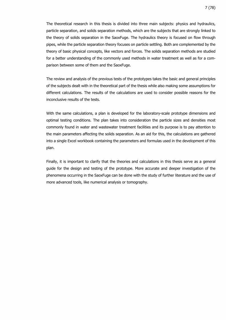
The sum of two or more vectors is called a resultant and these vectors become the resultant compo-
nents. The graphical sum of a vector is made by moving the vectors so that the end of one of the
vectors is the starting point of the next one. The resultant will be the vector that joins the starting
point of the first vector with the ending point of the last vector (Figure 2). Figure 2 also shows that
vector addition is commutative. (Benson 1995, 19; Tuomenlehto, Holmlund, Huuskonen, Makkonen
Surakka 2014, 169).
FIGURE 2. Graphical addition of two vectors
9 (78)
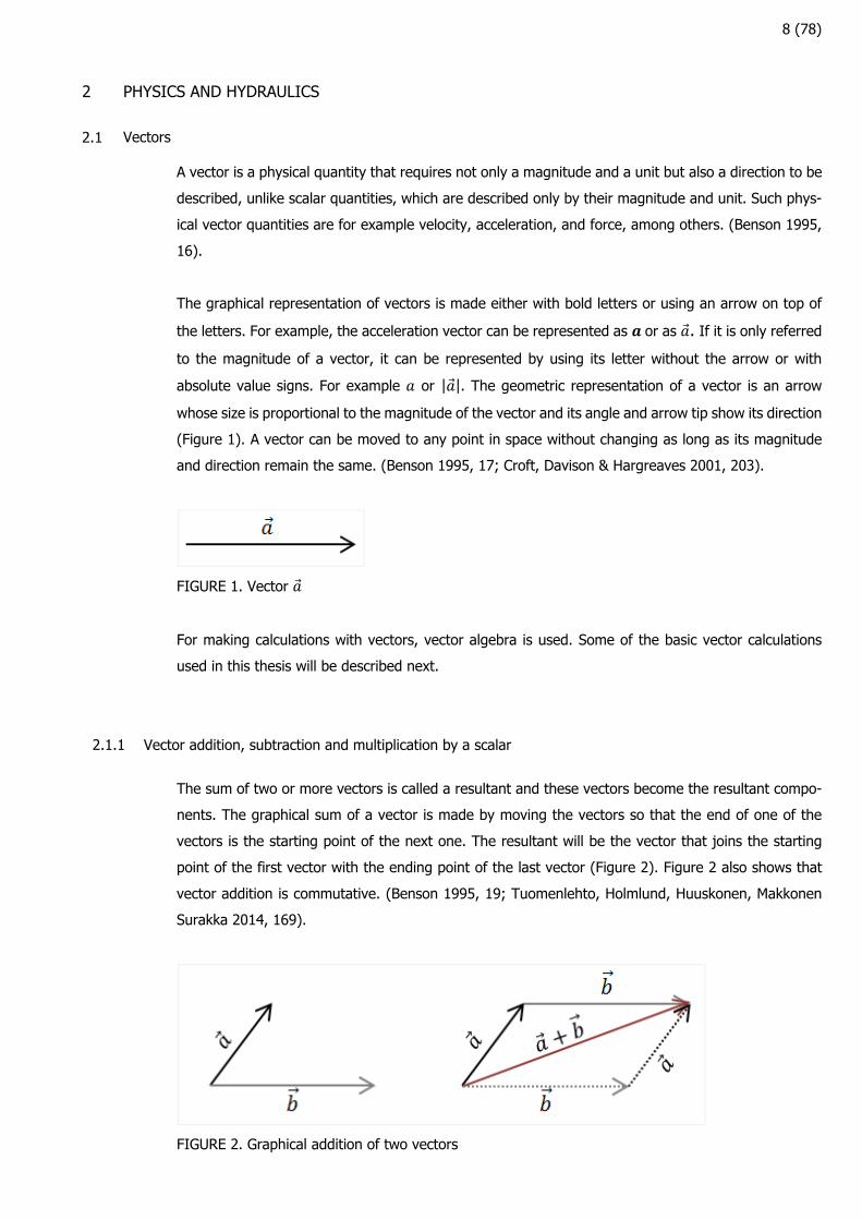
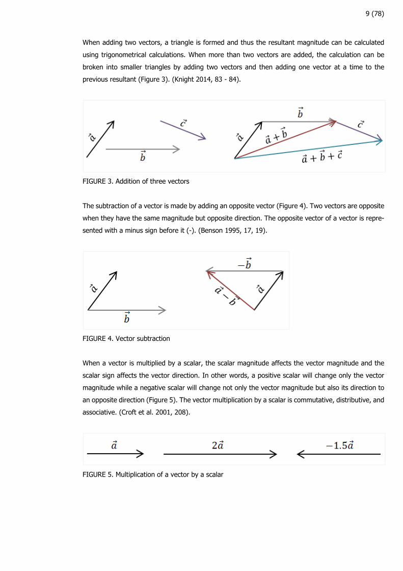
When adding two vectors, a triangle is formed and thus the resultant magnitude can be calculated
using trigonometrical calculations. When more than two vectors are added, the calculation can be
broken into smaller triangles by adding two vectors and then adding one vector at a time to the
previous resultant (Figure 3). (Knight 2014, 83 - 84).
FIGURE 3. Addition of three vectors
The subtraction of a vector is made by adding an opposite vector (Figure 4). Two vectors are opposite
when they have the same magnitude but opposite direction. The opposite vector of a vector is repre-
sented with a minus sign before it (-). (Benson 1995, 17, 19).
FIGURE 4. Vector subtraction
When a vector is multiplied by a scalar, the scalar magnitude affects the vector magnitude and the
scalar sign affects the vector direction. In other words, a positive scalar will change only the vector
magnitude while a negative scalar will change not only the vector magnitude but also its direction to
an opposite direction (Figure 5). The vector multiplication by a scalar is commutative, distributive, and
associative. (Croft et al. 2001, 208).
FIGURE 5. Multiplication of a vector by a scalar
10 (78)
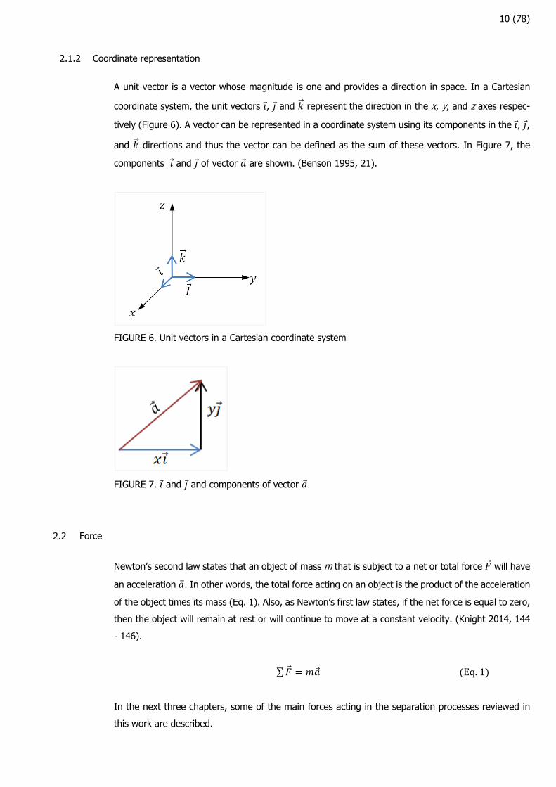
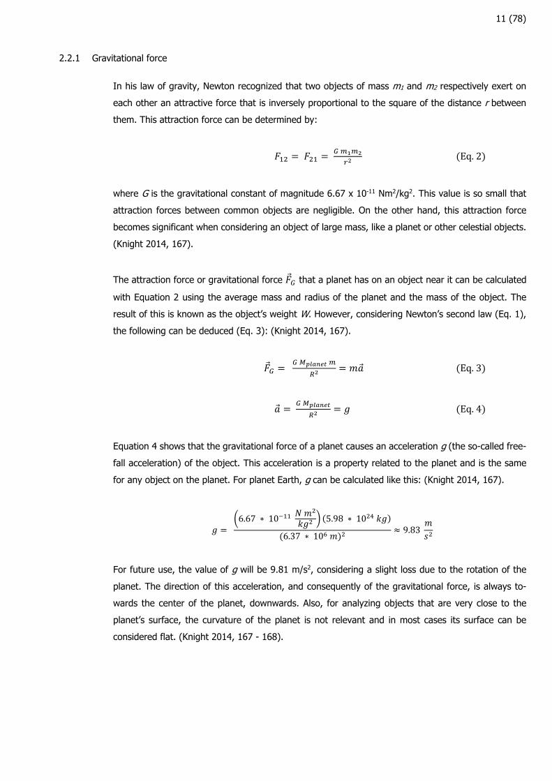
2.1.2 Coordinate representation
A unit vector is a vector whose magnitude is one and provides a direction in space. In a Cartesian
coordinate system, the unit vectors , and represent the direction in the x, y, and z axes respec-
tively (Figure 6). A vector can be represented in a coordinate system using its components in the , ,
and directions and thus the vector can be defined as the sum of these vectors. In Figure 7, the
components and of vector are shown. (Benson 1995, 21).
FIGURE 6. Unit vectors in a Cartesian coordinate system
FIGURE 7. and and components of vector
Force
Newton’s second law states that an object of mass m that is subject to a net or total force will have
an acceleration . In other words, the total force acting on an object is the product of the acceleration
of the object times its mass (Eq. 1). Also, as Newton’s first law states, if the net force is equal to zero,
then the object will remain at rest or will continue to move at a constant velocity. (Knight 2014, 144
- 146).
∑ Eq.1
In the next three chapters, some of the main forces acting in the separation processes reviewed in
this work are described.
11 (78)
2.2.1 Gravitational force
In his law of gravity, Newton recognized that two objects of mass m1 and m2 respectively exert on
each other an attractive force that is inversely proportional to the square of the distance r between
them. This attraction force can be determined by:
Eq.2
where G is the gravitational constant of magnitude 6.67 x 10⁻¹¹ Nm2/kg2. This value is so small that
attraction forces between common objects are negligible. On the other hand, this attraction force
becomes significant when considering an object of large mass, like a planet or other celestial objects.
(Knight 2014, 167).
The attraction force or gravitational force that a planet has on an object near it can be calculated
with Equation 2 using the average mass and radius of the planet and the mass of the object. The
result of this is known as the object’s weight W. However, considering Newton’s second law (Eq. 1),
the following can be deduced (Eq. 3): (Knight 2014, 167).
Eq.3
Eq.4
Equation 4 shows that the gravitational force of a planet causes an acceleration g (the so-called free-
fall acceleration) of the object. This acceleration is a property related to the planet and is the same
for any object on the planet. For planet Earth, g can be calculated like this: (Knight 2014, 167).
6.67 ∗ 10
5.98 ∗ 10
6.37 ∗ 10 9.83
For future use, the value of g will be 9.81 m/s2, considering a slight loss due to the rotation of the
planet. The direction of this acceleration, and consequently of the gravitational force, is always to-
wards the center of the planet, downwards. Also, for analyzing objects that are very close to the
planet’s surface, the curvature of the planet is not relevant and in most cases its surface can be
considered flat. (Knight 2014, 167 - 168).
12 (78)
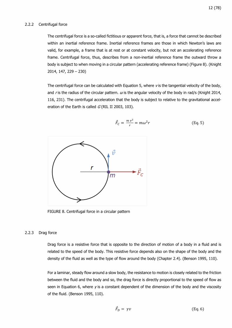
2.2.2 Centrifugal force
The centrifugal force is a so-called fictitious or apparent force, that is, a force that cannot be described
within an inertial reference frame. Inertial reference frames are those in which Newton’s laws are
valid, for example, a frame that is at rest or at constant velocity, but not an accelerating reference
frame. Centrifugal force, thus, describes from a non-inertial reference frame the outward throw a
body is subject to when moving in a circular pattern (accelerating reference frame) (Figure 8). (Knight
2014, 147, 229 – 230)
The centrifugal force can be calculated with Equation 5, where v is the tangential velocity of the body,
and r is the radius of the circular pattern. ω is the angular velocity of the body in rad/s (Knight 2014,
116, 231). The centrifugal acceleration that the body is subject to relative to the gravitational accel-
eration of the Earth is called G (RIL II 2003, 103).
Eq.5
FIGURE 8. Centrifugal force in a circular pattern
2.2.3 Drag force
Drag force is a resistive force that is opposite to the direction of motion of a body in a fluid and is
related to the speed of the body. This resistive force depends also on the shape of the body and the
density of the fluid as well as the type of flow around the body (Chapter 2.4). (Benson 1995, 110).
For a laminar, steady flow around a slow body, the resistance to motion is closely related to the friction
between the fluid and the body and so, the drag force is directly proportional to the speed of flow as
seen in Equation 6, where γ is a constant dependent of the dimension of the body and the viscosity
of the fluid. (Benson 1995, 110).
Eq.6
13 (78)
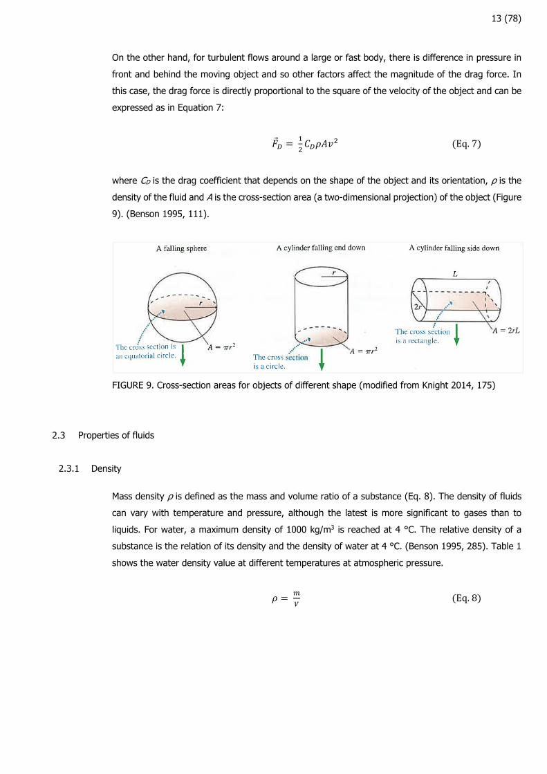
On the other hand, for turbulent flows around a large or fast body, there is difference in pressure in
front and behind the moving object and so other factors affect the magnitude of the drag force. In
this case, the drag force is directly proportional to the square of the velocity of the object and can be
expressed as in Equation 7:
Eq.7
where CD is the drag coefficient that depends on the shape of the object and its orientation, ρ is the
density of the fluid and A is the cross-section area (a two-dimensional projection) of the object (Figure
9). (Benson 1995, 111).
FIGURE 9. Cross-section areas for objects of different shape (modified from Knight 2014, 175)
Properties of fluids
2.3.1 Density
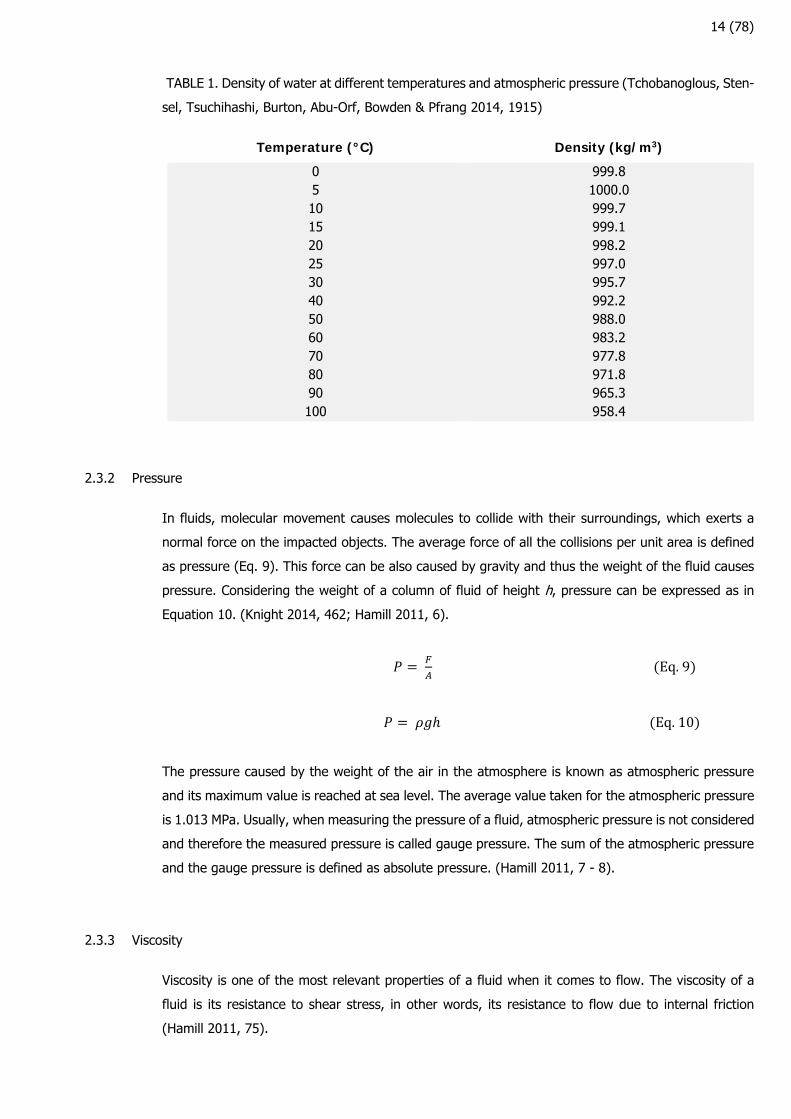
Mass density ρ is defined as the mass and volume ratio of a substance (Eq. 8). The density of fluids
can vary with temperature and pressure, although the latest is more significant to gases than to
liquids. For water, a maximum density of 1000 kg/m3 is reached at 4 °C. The relative density of a
substance is the relation of its density and the density of water at 4 °C. (Benson 1995, 285). Table 1
shows the water density value at different temperatures at atmospheric pressure.
Eq.8
14 (78)
TABLE 1. Density of water at different temperatures and atmospheric pressure (Tchobanoglous, Sten-
sel, Tsuchihashi, Burton, Abu-Orf, Bowden & Pfrang 2014, 1915)
Temperature (°C) Density (kg/m3)
0 5 10 15 20 25 30 40 50 60 70 80 90 100
999.8 1000.0 999.7 999.1 998.2 997.0 995.7 992.2 988.0 983.2 977.8 971.8 965.3 958.4
2.3.2 Pressure
In fluids, molecular movement causes molecules to collide with their surroundings, which exerts a
normal force on the impacted objects. The average force of all the collisions per unit area is defined
as pressure (Eq. 9). This force can be also caused by gravity and thus the weight of the fluid causes
pressure. Considering the weight of a column of fluid of height h, pressure can be expressed as in
Equation 10. (Knight 2014, 462; Hamill 2011, 6).
Eq.9
Eq.10
The pressure caused by the weight of the air in the atmosphere is known as atmospheric pressure
and its maximum value is reached at sea level. The average value taken for the atmospheric pressure
is 1.013 MPa. Usually, when measuring the pressure of a fluid, atmospheric pressure is not considered
and therefore the measured pressure is called gauge pressure. The sum of the atmospheric pressure
and the gauge pressure is defined as absolute pressure. (Hamill 2011, 7 - 8).
2.3.3 Viscosity
Viscosity is one of the most relevant properties of a fluid when it comes to flow. The viscosity of a
fluid is its resistance to shear stress, in other words, its resistance to flow due to internal friction
(Hamill 2011, 75).
15 (78)
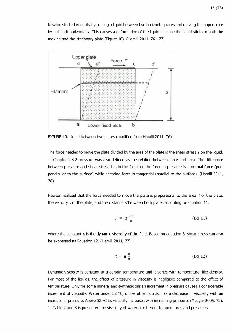
Newton studied viscosity by placing a liquid between two horizontal plates and moving the upper plate
by pulling it horizontally. This causes a deformation of the liquid because the liquid sticks to both the
moving and the stationary plate (Figure 10). (Hamill 2011, 76 - 77).
FIGURE 10. Liquid between two plates (modified from Hamill 2011, 76)
The force needed to move the plate divided by the area of the plate is the shear stress on the liquid.
In Chapter 2.3.2 pressure was also defined as the relation between force and area. The difference
between pressure and shear stress lies in the fact that the force in pressure is a normal force (per-
pendicular to the surface) while shearing force is tangential (parallel to the surface). (Hamill 2011,
76)
Newton realized that the force needed to move the plate is proportional to the area A of the plate,
the velocity v of the plate, and the distance d between both plates according to Equation 11:
Eq.11
where the constant µ is the dynamic viscosity of the fluid. Based on equation 8, shear stress can also
be expressed as Equation 12. (Hamill 2011, 77).
Eq.12
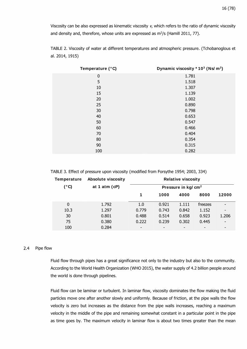
Dynamic viscosity is constant at a certain temperature and it varies with temperature, like density.
For most of the liquids, the effect of pressure in viscosity is negligible compared to the effect of
temperature. Only for some mineral and synthetic oils an increment in pressure causes a considerable
increment of viscosity. Water under 32 °C, unlike other liquids, has a decrease in viscosity with an
increase of pressure. Above 32 °C its viscosity increases with increasing pressure. (Mezger 2006, 72).
In Table 2 and 3 is presented the viscosity of water at different temperatures and pressures.
16 (78)
Viscosity can be also expressed as kinematic viscosity v, which refers to the ratio of dynamic viscosity
and density and, therefore, whose units are expressed as m2/s (Hamill 2011, 77).
TABLE 2. Viscosity of water at different temperatures and atmospheric pressure. (Tchobanoglous et
al. 2014, 1915)
Temperature (°C) Dynamic viscosity *103 (Ns/m2)
0 5 10 15 20 25 30 40 50 60 70 80 90 100
1.781 1.518 1.307 1.139 1.002 0.890 0.798 0.653 0.547 0.466 0.404 0.354 0.315 0.282
TABLE 3. Effect of pressure upon viscosity (modified from Forsythe 1954; 2003, 334)
Temperature
(°C)
Absolute viscosity
at 1 atm (cP)
Relative viscosity
Pressure in kg/cm2
1 1000 4000 8000 12000
0 10.3 30 75 100
1.792 1.297 0.801 0.380 0.284
1.0 0.779 0.488 0.222
-
0.921 0.743 0.514 0.239
-
1.111 0.842 0.658 0.302
-
freezes 1.152 0.923 0.445
-
- -
1.206 - -
Pipe flow
Fluid flow through pipes has a great significance not only to the industry but also to the community.
According to the World Health Organization (WHO 2015), the water supply of 4.2 billion people around
the world is done through pipelines.
Fluid flow can be laminar or turbulent. In laminar flow, viscosity dominates the flow making the fluid
particles move one after another slowly and uniformly. Because of friction, at the pipe walls the flow
velocity is zero but increases as the distance from the pipe walls increases, reaching a maximum
velocity in the middle of the pipe and remaining somewhat constant in a particular point in the pipe
as time goes by. The maximum velocity in laminar flow is about two times greater than the mean
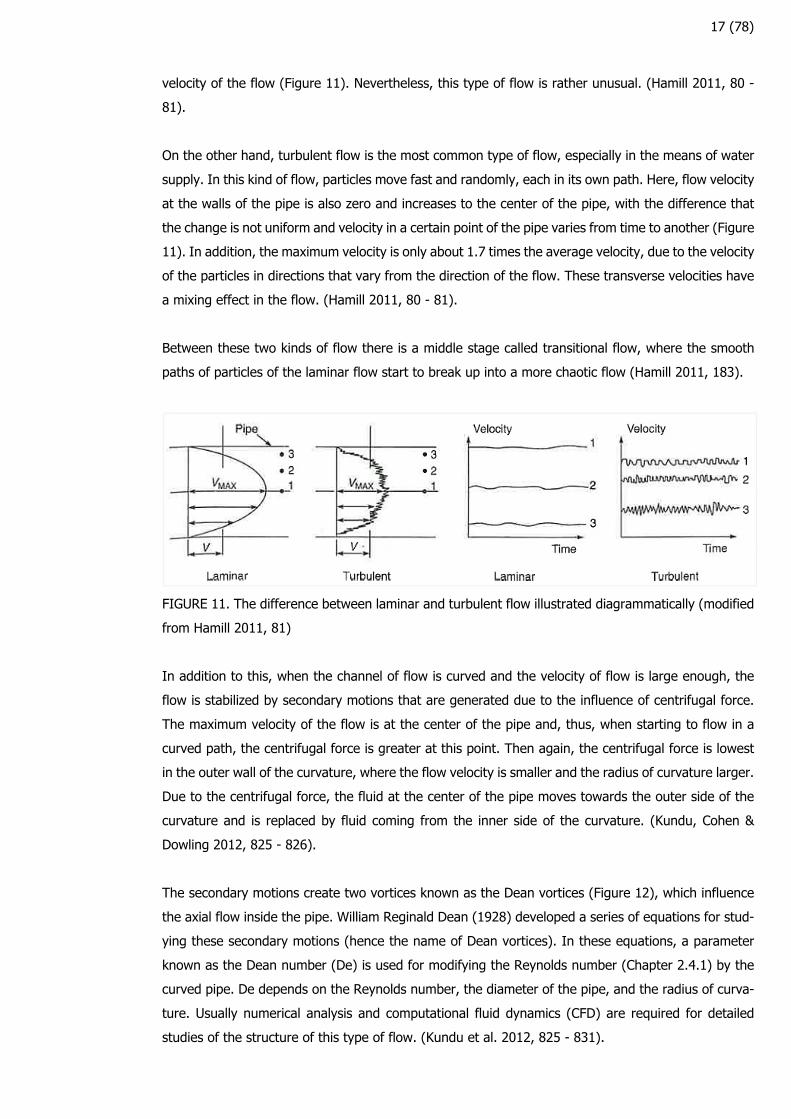
17 (78)
velocity of the flow (Figure 11). Nevertheless, this type of flow is rather unusual. (Hamill 2011, 80 -
81).
On the other hand, turbulent flow is the most common type of flow, especially in the means of water
supply. In this kind of flow, particles move fast and randomly, each in its own path. Here, flow velocity
at the walls of the pipe is also zero and increases to the center of the pipe, with the difference that
the change is not uniform and velocity in a certain point of the pipe varies from time to another (Figure
11). In addition, the maximum velocity is only about 1.7 times the average velocity, due to the velocity
of the particles in directions that vary from the direction of the flow. These transverse velocities have
a mixing effect in the flow. (Hamill 2011, 80 - 81).
Between these two kinds of flow there is a middle stage called transitional flow, where the smooth
paths of particles of the laminar flow start to break up into a more chaotic flow (Hamill 2011, 183).
FIGURE 11. The difference between laminar and turbulent flow illustrated diagrammatically (modified
from Hamill 2011, 81)
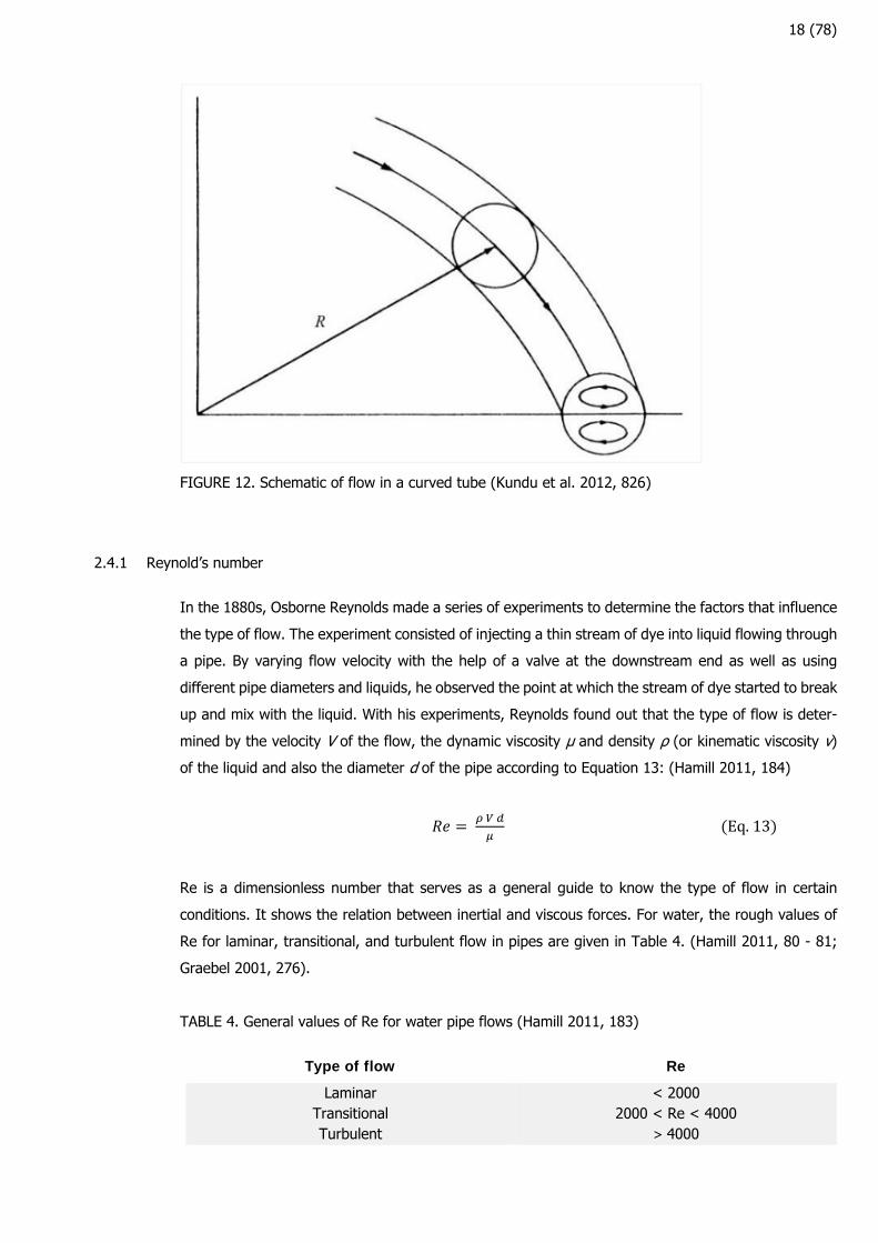
In addition to this, when the channel of flow is curved and the velocity of flow is large enough, the
flow is stabilized by secondary motions that are generated due to the influence of centrifugal force.
The maximum velocity of the flow is at the center of the pipe and, thus, when starting to flow in a
curved path, the centrifugal force is greater at this point. Then again, the centrifugal force is lowest
in the outer wall of the curvature, where the flow velocity is smaller and the radius of curvature larger.
Due to the centrifugal force, the fluid at the center of the pipe moves towards the outer side of the
curvature and is replaced by fluid coming from the inner side of the curvature. (Kundu, Cohen &
Dowling 2012, 825 - 826).
The secondary motions create two vortices known as the Dean vortices (Figure 12), which influence
the axial flow inside the pipe. William Reginald Dean (1928) developed a series of equations for stud-
ying these secondary motions (hence the name of Dean vortices). In these equations, a parameter
known as the Dean number (De) is used for modifying the Reynolds number (Chapter 2.4.1) by the
curved pipe. De depends on the Reynolds number, the diameter of the pipe, and the radius of curva-
ture. Usually numerical analysis and computational fluid dynamics (CFD) are required for detailed
studies of the structure of this type of flow. (Kundu et al. 2012, 825 - 831).
18 (78)
FIGURE 12. Schematic of flow in a curved tube (Kundu et al. 2012, 826)
2.4.1 Reynold’s number
In the 1880s, Osborne Reynolds made a series of experiments to determine the factors that influence
the type of flow. The experiment consisted of injecting a thin stream of dye into liquid flowing through
a pipe. By varying flow velocity with the help of a valve at the downstream end as well as using
different pipe diameters and liquids, he observed the point at which the stream of dye started to break
up and mix with the liquid. With his experiments, Reynolds found out that the type of flow is deter-
mined by the velocity V of the flow, the dynamic viscosity µ and density ρ (or kinematic viscosity v)
of the liquid and also the diameter d of the pipe according to Equation 13: (Hamill 2011, 184)
Eq.13
Re is a dimensionless number that serves as a general guide to know the type of flow in certain
conditions. It shows the relation between inertial and viscous forces. For water, the rough values of
Re for laminar, transitional, and turbulent flow in pipes are given in Table 4. (Hamill 2011, 80 - 81;
Graebel 2001, 276).
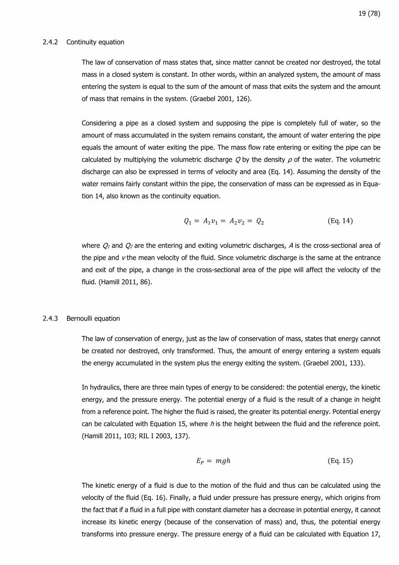
TABLE 4. General values of Re for water pipe flows (Hamill 2011, 183)
Type of flow Re
Laminar Transitional Turbulent
< 2000 2000 < Re < 4000
> 4000
19 (78)
2.4.2 Continuity equation
The law of conservation of mass states that, since matter cannot be created nor destroyed, the total
mass in a closed system is constant. In other words, within an analyzed system, the amount of mass
entering the system is equal to the sum of the amount of mass that exits the system and the amount
of mass that remains in the system. (Graebel 2001, 126).
Considering a pipe as a closed system and supposing the pipe is completely full of water, so the
amount of mass accumulated in the system remains constant, the amount of water entering the pipe
equals the amount of water exiting the pipe. The mass flow rate entering or exiting the pipe can be
calculated by multiplying the volumetric discharge Q by the density ρ of the water. The volumetric
discharge can also be expressed in terms of velocity and area (Eq. 14). Assuming the density of the
water remains fairly constant within the pipe, the conservation of mass can be expressed as in Equa-
tion 14, also known as the continuity equation.
Eq.14
where Q1 and Q2 are the entering and exiting volumetric discharges, A is the cross-sectional area of
the pipe and v the mean velocity of the fluid. Since volumetric discharge is the same at the entrance
and exit of the pipe, a change in the cross-sectional area of the pipe will affect the velocity of the
fluid. (Hamill 2011, 86).
2.4.3 Bernoulli equation
The law of conservation of energy, just as the law of conservation of mass, states that energy cannot
be created nor destroyed, only transformed. Thus, the amount of energy entering a system equals
the energy accumulated in the system plus the energy exiting the system. (Graebel 2001, 133).
In hydraulics, there are three main types of energy to be considered: the potential energy, the kinetic
energy, and the pressure energy. The potential energy of a fluid is the result of a change in height
from a reference point. The higher the fluid is raised, the greater its potential energy. Potential energy
can be calculated with Equation 15, where h is the height between the fluid and the reference point.
(Hamill 2011, 103; RIL I 2003, 137).
Eq.15
The kinetic energy of a fluid is due to the motion of the fluid and thus can be calculated using the
velocity of the fluid (Eq. 16). Finally, a fluid under pressure has pressure energy, which origins from
the fact that if a fluid in a full pipe with constant diameter has a decrease in potential energy, it cannot
increase its kinetic energy (because of the conservation of mass) and, thus, the potential energy
transforms into pressure energy. The pressure energy of a fluid can be calculated with Equation 17,
20 (78)
where p is the pressure of the fluid, A is the cross-sectional area of the pipe and L is the distance that
the fluid has travelled. (Hamill 2011, 103).
Eq.16
Eq.17
The total energy in the pipe is the sum of the three types of energy and it has to remain constant in
both ends of the pipe analyzed. Also, the amount of energy is usually expressed per unit weight of
fluid (W = mg), and therefore its unit is expressed in meters. The energy terms given in meters are
called heads: the elevation, velocity, and pressure heads. The amount of energy between two points
in a pipe can be expressed as in Equation 18, the so-called energy equation or Bernoulli equation:
(Hamill 2011, 103 - 105, 164; RIL I 2003, 137)
Eq.18
The last equation is valid assuming there are no energy losses due to factors like friction or bends,
among others. Hence, for a real fluid and flow, the energy head losses term (hf) can be added to the
Bernoulli equation and be expressed as in Equation 19. In Chapter 2.4.4 head losses calculation is
described. (Hamill 2011, 105).
Eq.19
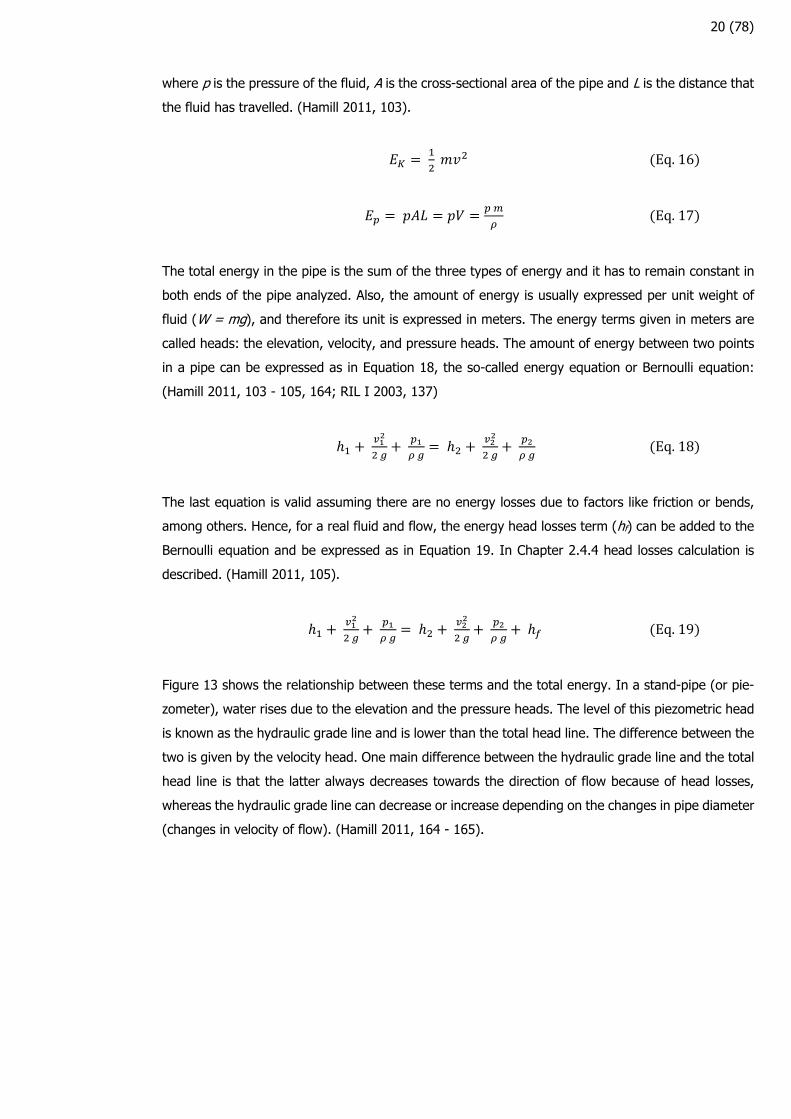
Figure 13 shows the relationship between these terms and the total energy. In a stand-pipe (or pie-
zometer), water rises due to the elevation and the pressure heads. The level of this piezometric head
is known as the hydraulic grade line and is lower than the total head line. The difference between the
two is given by the velocity head. One main difference between the hydraulic grade line and the total
head line is that the latter always decreases towards the direction of flow because of head losses,
whereas the hydraulic grade line can decrease or increase depending on the changes in pipe diameter
(changes in velocity of flow). (Hamill 2011, 164 - 165).
21 (78)
FIGURE 13. Water pipe flow and its energy types (modified from RIL I 2003, 137)
2.4.4 Head loss
The head losses (hf) mentioned in the previous chapter can be caused by friction between the water
and the pipe (friction losses), or minor losses caused by changes in the cross-sectional area of flow,
pipe diameter, bends, and fittings. Usually, friction losses would be more significant in long pipes,
while minor losses would be more significant in short pipes. (Hamill 2011, 169).
Some of the methods and equations for calculation of the head losses will be described next.
Poiseuille equation
In the 1840’s, Jean Louis Poiseuille developed an equation for the calculation of friction loss in laminar
flow (Eq. 20). In this type of flow, head losses due to friction are proportional to the velocity of the
flow and pipe roughness does not affect the flow, so in Poiseuille’s equation is expressed that head
losses hF in laminar flow depend on the kinematic viscosity v of the fluid, the length L and diameter
D of the pipe, and the mean velocity V of the flow. (Hamill 2011, 185).
Eq.20
22 (78)
Darcy-Weisbach equation
Around 1850, Henry Darcy and Julius Weisbach developed an equation for determining head losses
in full pipes. Unlike in laminar flow, the head loss in turbulent flow is directly proportional to the square
of the velocity. The Darcy-Weisbach equation considers this and also the effect of pipe roughness on
the flow (Equation 21).
Eq.21
where f is the pipe friction factor, L is the length of the pipe, V is the mean velocity of the flow, and
D is the inner diameter of the pipe. (Hamill 2011, 185; RIL I 2003, 140).
The friction factor value depends mainly on the Reynolds number and the relative pipe roughness.
For laminar flow, the viscosity of the fluid is the main factor affecting the friction factor, so equating
the Poiseuille equation with the Darcy-Weisbach equation, the friction factor can be calculated with
Equation 22: (Hamill 2001, 186)
Eq.22
Johann Nikuradse experimented in 1933 the effect of pipe roughness on head loss by gluing grains of
sand of known size (k) to the walls of a pipe and measuring the discharge. The relation between the
size of the grains of sand and the diameter of the pipe is known as the relative roughness of the pipe.
The results of these experiments were later compared to the results of tests with commercial pipes.
In 1938-1939, Frank Colebrook realized that Nikuradse’s experiment results could be expressed with
the formula in Equation 23. Lewis Moody graphed in 1944 the results of this formula, resulting in what
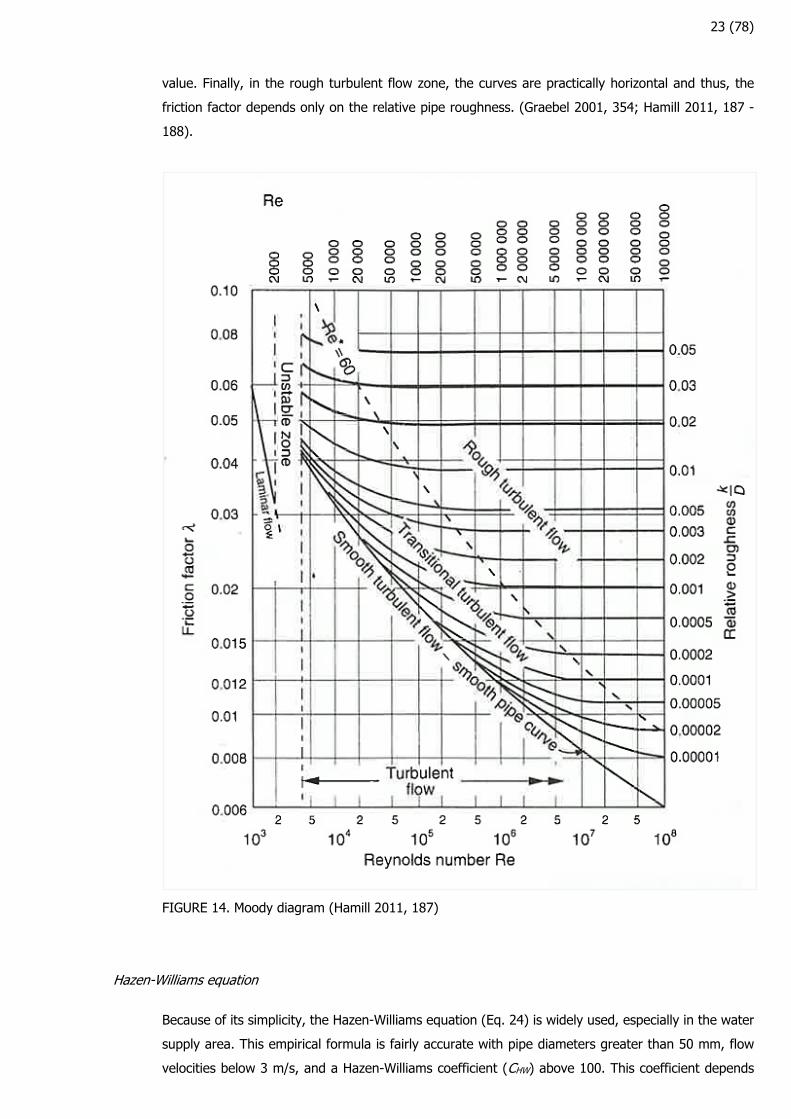
is called the Moody diagram (Figure 14), which can be used to determine the friction factor f. (Graebel
2001, 354; Hamill 2011, 186 - 187).
2 log .
.
Eq.23
The Moody diagram shows the friction factor values for the laminar flow (Eq. 22), as well as a critical
zone, and three different zones of turbulent flow: the smooth turbulent flow, the transitional turbulent
flow, and the rough turbulent flow (Graebel 2001, 354).
The critical zone corresponds to Reynolds number values of 2300 to about 4000, where the type of
flow is transitional, and thus it is difficult to determine accurately the friction factor in this area. The
smooth turbulent flow zone is at the bottom of the diagram. In this, the pipe roughness does not have
yet significance and the curve depends on the Reynolds number. In the transitional turbulent flow,
the curves of different relative roughness values start to separate from the smooth turbulent flow
curve, so both the Reynolds number and the relative roughness of the pipe affect the friction factor
23 (78)
value. Finally, in the rough turbulent flow zone, the curves are practically horizontal and thus, the
friction factor depends only on the relative pipe roughness. (Graebel 2001, 354; Hamill 2011, 187 -
188).
FIGURE 14. Moody diagram (Hamill 2011, 187)
Hazen-Williams equation
Because of its simplicity, the Hazen-Williams equation (Eq. 24) is widely used, especially in the water
supply area. This empirical formula is fairly accurate with pipe diameters greater than 50 mm, flow
velocities below 3 m/s, and a Hazen-Williams coefficient (CHW) above 100. This coefficient depends
24 (78)
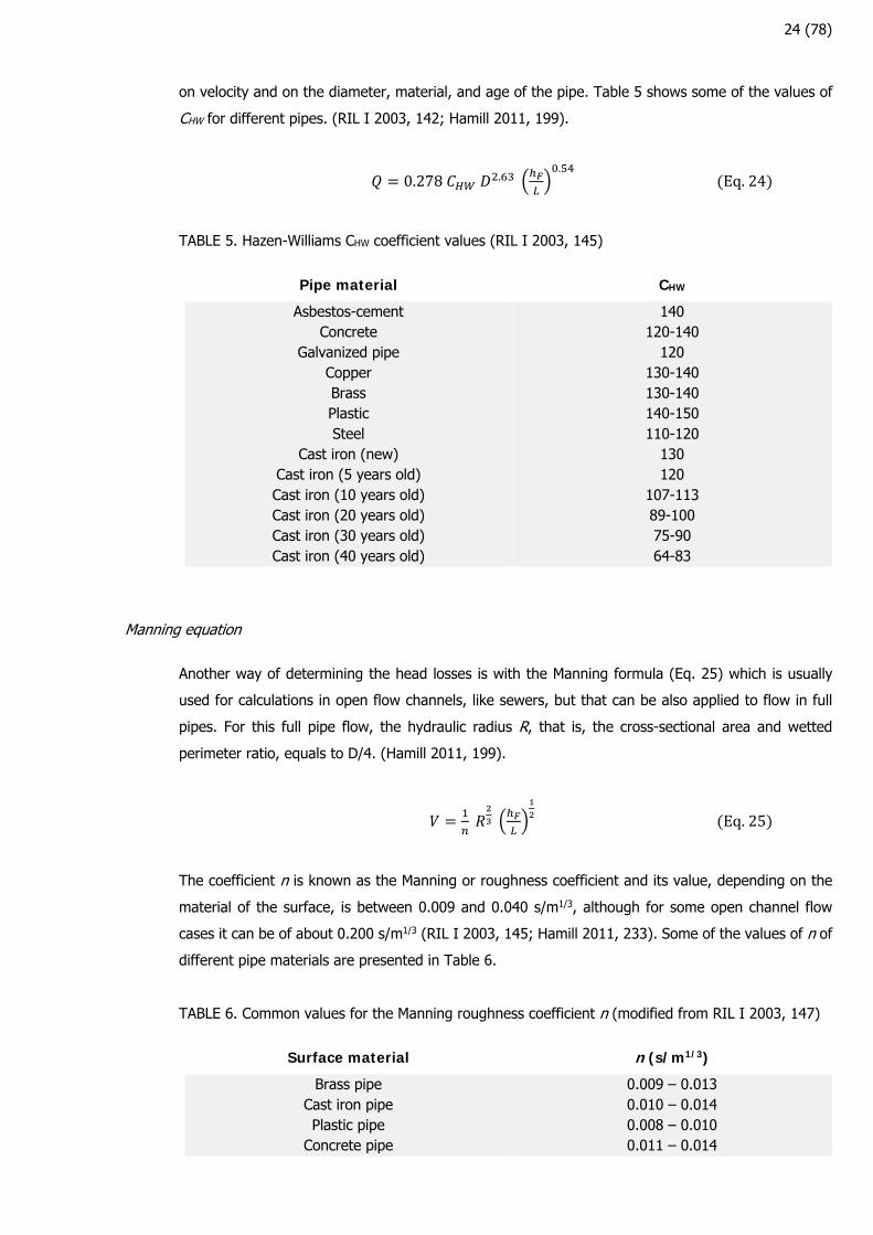
on velocity and on the diameter, material, and age of the pipe. Table 5 shows some of the values of
CHW for different pipes. (RIL I 2003, 142; Hamill 2011, 199).
0.278 . .
Eq.24
TABLE 5. Hazen-Williams CHW coefficient values (RIL I 2003, 145)
Pipe material CHW
Asbestos-cement Concrete
Galvanized pipe Copper Brass Plastic Steel
Cast iron (new) Cast iron (5 years old) Cast iron (10 years old) Cast iron (20 years old) Cast iron (30 years old) Cast iron (40 years old)
140 120-140
120 130-140 130-140 140-150 110-120
130 120
107-113 89-100 75-90 64-83
Manning equation
Another way of determining the head losses is with the Manning formula (Eq. 25) which is usually
used for calculations in open flow channels, like sewers, but that can be also applied to flow in full
pipes. For this full pipe flow, the hydraulic radius R, that is, the cross-sectional area and wetted
perimeter ratio, equals to D/4. (Hamill 2011, 199).
Eq.25
The coefficient n is known as the Manning or roughness coefficient and its value, depending on the
material of the surface, is between 0.009 and 0.040 s/m1/3, although for some open channel flow
cases it can be of about 0.200 s/m1/3 (RIL I 2003, 145; Hamill 2011, 233). Some of the values of n of
different pipe materials are presented in Table 6.
TABLE 6. Common values for the Manning roughness coefficient n (modified from RIL I 2003, 147)
Surface material n (s/m1/3)
Brass pipe Cast iron pipe Plastic pipe
Concrete pipe
0.009 – 0.013 0.010 – 0.014 0.008 – 0.010 0.011 – 0.014
25 (78)
Minor losses
Minor head losses are caused by changes in pipe diameter and cross-sectional area, as well as fittings
like valves and bends. Although called minor losses, these head losses can be of great significance,
especially in short pipes. (Hamill 2011, 169).
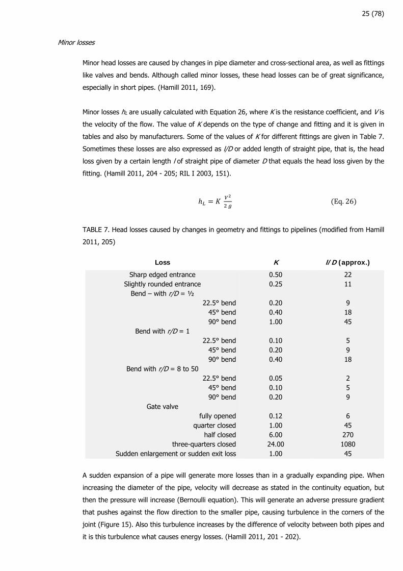
Minor losses hL are usually calculated with Equation 26, where K is the resistance coefficient, and V is
the velocity of the flow. The value of K depends on the type of change and fitting and it is given in
tables and also by manufacturers. Some of the values of K for different fittings are given in Table 7.
Sometimes these losses are also expressed as l/D or added length of straight pipe, that is, the head
loss given by a certain length l of straight pipe of diameter D that equals the head loss given by the
fitting. (Hamill 2011, 204 - 205; RIL I 2003, 151).
Eq.26
TABLE 7. Head losses caused by changes in geometry and fittings to pipelines (modified from Hamill
2011, 205)
Loss K l/D (approx.)
Sharp edged entrance Slightly rounded entrance
Bend – with r/D = ½ 22.5° bend
45° bend90° bend
Bend with r/D = 1 22.5° bend
45° bend90° bend
Bend with r/D = 8 to 50 22.5° bend
45° bend90° bend
Gate valve fully opened
quarter closedhalf closed
three-quarters closedSudden enlargement or sudden exit loss
0.50 0.25
0.20 0.40 1.00
0.10 0.20 0.40
0.05 0.10 0.20
0.12 1.00 6.00 24.00 1.00
22 11 9 18 45 5 9 18 2 5 9 6 45 270 1080 45
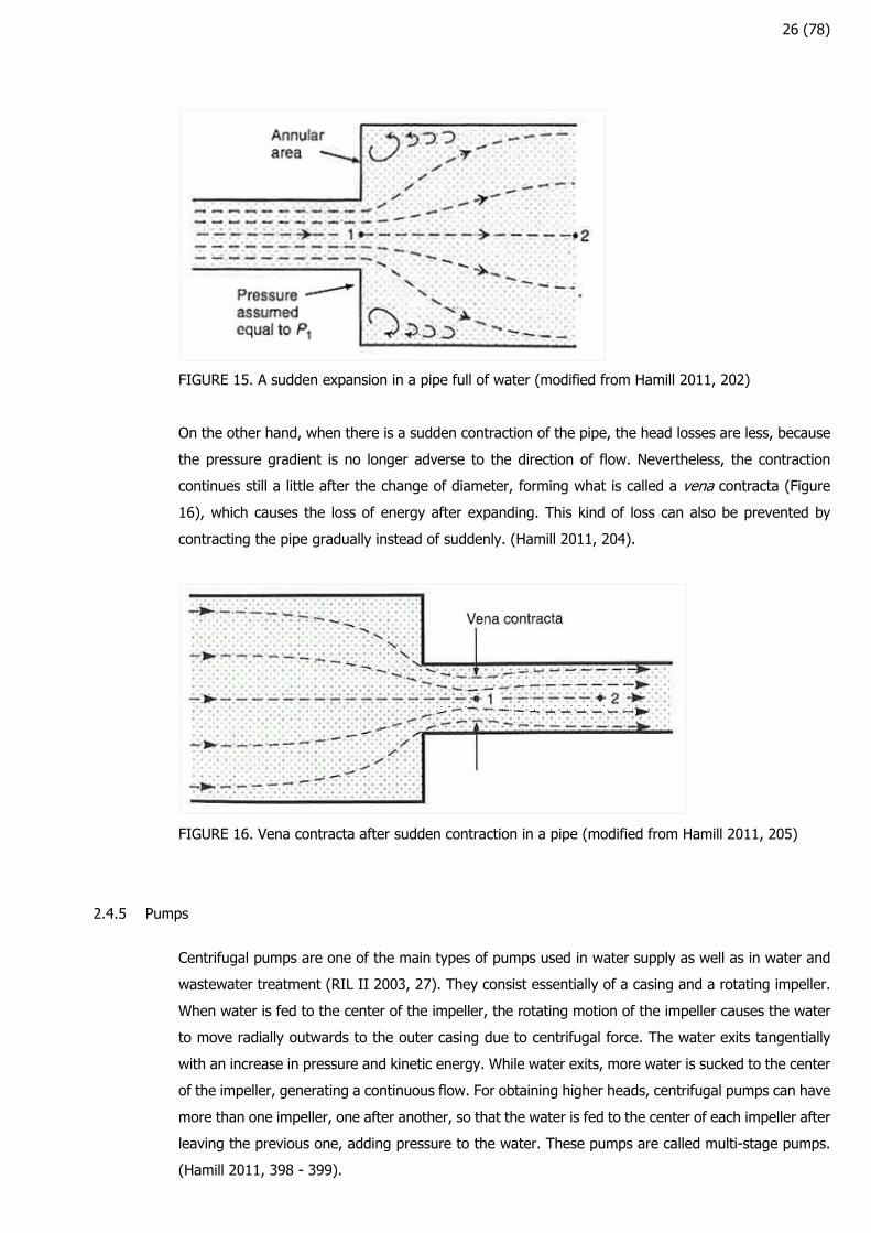
A sudden expansion of a pipe will generate more losses than in a gradually expanding pipe. When
increasing the diameter of the pipe, velocity will decrease as stated in the continuity equation, but
then the pressure will increase (Bernoulli equation). This will generate an adverse pressure gradient
that pushes against the flow direction to the smaller pipe, causing turbulence in the corners of the
joint (Figure 15). Also this turbulence increases by the difference of velocity between both pipes and
it is this turbulence what causes energy losses. (Hamill 2011, 201 - 202).
26 (78)
FIGURE 15. A sudden expansion in a pipe full of water (modified from Hamill 2011, 202)
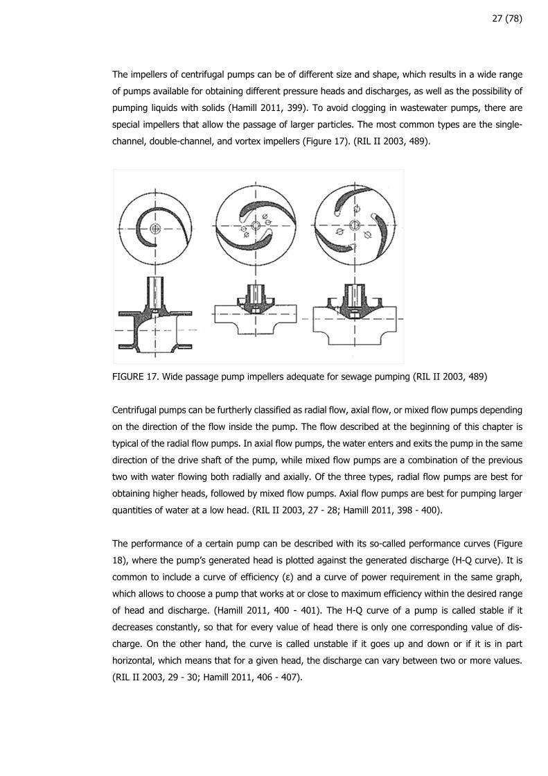
On the other hand, when there is a sudden contraction of the pipe, the head losses are less, because
the pressure gradient is no longer adverse to the direction of flow. Nevertheless, the contraction
continues still a little after the change of diameter, forming what is called a vena contracta (Figure
16), which causes the loss of energy after expanding. This kind of loss can also be prevented by
contracting the pipe gradually instead of suddenly. (Hamill 2011, 204).
FIGURE 16. Vena contracta after sudden contraction in a pipe (modified from Hamill 2011, 205)
2.4.5 Pumps
Centrifugal pumps are one of the main types of pumps used in water supply as well as in water and
wastewater treatment (RIL II 2003, 27). They consist essentially of a casing and a rotating impeller.
When water is fed to the center of the impeller, the rotating motion of the impeller causes the water
to move radially outwards to the outer casing due to centrifugal force. The water exits tangentially
with an increase in pressure and kinetic energy. While water exits, more water is sucked to the center
of the impeller, generating a continuous flow. For obtaining higher heads, centrifugal pumps can have
more than one impeller, one after another, so that the water is fed to the center of each impeller after
leaving the previous one, adding pressure to the water. These pumps are called multi-stage pumps.
(Hamill 2011, 398 - 399).
27 (78)
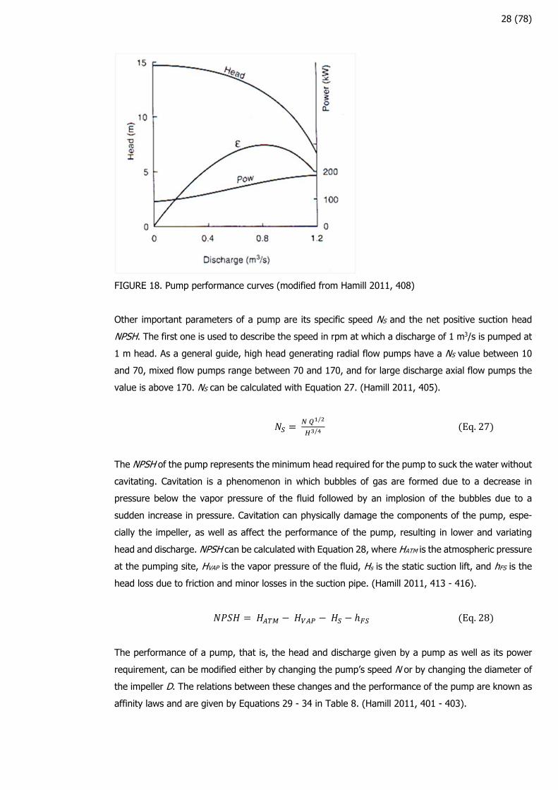
The impellers of centrifugal pumps can be of different size and shape, which results in a wide range
of pumps available for obtaining different pressure heads and discharges, as well as the possibility of
pumping liquids with solids (Hamill 2011, 399). To avoid clogging in wastewater pumps, there are
special impellers that allow the passage of larger particles. The most common types are the single-
channel, double-channel, and vortex impellers (Figure 17). (RIL II 2003, 489).
FIGURE 17. Wide passage pump impellers adequate for sewage pumping (RIL II 2003, 489)
Centrifugal pumps can be furtherly classified as radial flow, axial flow, or mixed flow pumps depending
on the direction of the flow inside the pump. The flow described at the beginning of this chapter is
typical of the radial flow pumps. In axial flow pumps, the water enters and exits the pump in the same
direction of the drive shaft of the pump, while mixed flow pumps are a combination of the previous
two with water flowing both radially and axially. Of the three types, radial flow pumps are best for
obtaining higher heads, followed by mixed flow pumps. Axial flow pumps are best for pumping larger
quantities of water at a low head. (RIL II 2003, 27 - 28; Hamill 2011, 398 - 400).
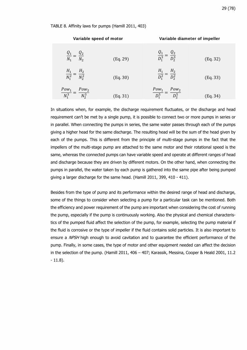
The performance of a certain pump can be described with its so-called performance curves (Figure
18), where the pump’s generated head is plotted against the generated discharge (H-Q curve). It is
common to include a curve of efficiency (ε) and a curve of power requirement in the same graph,
which allows to choose a pump that works at or close to maximum efficiency within the desired range
of head and discharge. (Hamill 2011, 400 - 401). The H-Q curve of a pump is called stable if it
decreases constantly, so that for every value of head there is only one corresponding value of dis-
charge. On the other hand, the curve is called unstable if it goes up and down or if it is in part
horizontal, which means that for a given head, the discharge can vary between two or more values.
(RIL II 2003, 29 - 30; Hamill 2011, 406 - 407).
28 (78)
FIGURE 18. Pump performance curves (modified from Hamill 2011, 408)
Other important parameters of a pump are its specific speed NS and the net positive suction head
NPSH. The first one is used to describe the speed in rpm at which a discharge of 1 m3/s is pumped at
1 m head. As a general guide, high head generating radial flow pumps have a NS value between 10
and 70, mixed flow pumps range between 70 and 170, and for large discharge axial flow pumps the
value is above 170. NS can be calculated with Equation 27. (Hamill 2011, 405).
/
/ Eq.27
The NPSH of the pump represents the minimum head required for the pump to suck the water without
cavitating. Cavitation is a phenomenon in which bubbles of gas are formed due to a decrease in
pressure below the vapor pressure of the fluid followed by an implosion of the bubbles due to a
sudden increase in pressure. Cavitation can physically damage the components of the pump, espe-
cially the impeller, as well as affect the performance of the pump, resulting in lower and variating
head and discharge. NPSH can be calculated with Equation 28, where HATM is the atmospheric pressure
at the pumping site, HVAP is the vapor pressure of the fluid, Hs is the static suction lift, and hFS is the
head loss due to friction and minor losses in the suction pipe. (Hamill 2011, 413 - 416).
Eq.28
The performance of a pump, that is, the head and discharge given by a pump as well as its power
requirement, can be modified either by changing the pump’s speed N or by changing the diameter of
the impeller D. The relations between these changes and the performance of the pump are known as
affinity laws and are given by Equations 29 - 34 in Table 8. (Hamill 2011, 401 - 403).
29 (78)
TABLE 8. Affinity laws for pumps (Hamill 2011, 403)
Variable speed of motor Variable diameter of impeller
Eq.29
Eq.30
Eq.31
Eq.32
Eq.33
Eq.34
In situations when, for example, the discharge requirement fluctuates, or the discharge and head
requirement can’t be met by a single pump, it is possible to connect two or more pumps in series or
in parallel. When connecting the pumps in series, the same water passes through each of the pumps
giving a higher head for the same discharge. The resulting head will be the sum of the head given by
each of the pumps. This is different from the principle of multi-stage pumps in the fact that the
impellers of the multi-stage pump are attached to the same motor and their rotational speed is the
same, whereas the connected pumps can have variable speed and operate at different ranges of head
and discharge because they are driven by different motors. On the other hand, when connecting the
pumps in parallel, the water taken by each pump is gathered into the same pipe after being pumped
giving a larger discharge for the same head. (Hamill 2011, 399, 410 - 411).
Besides from the type of pump and its performance within the desired range of head and discharge,
some of the things to consider when selecting a pump for a particular task can be mentioned. Both
the efficiency and power requirement of the pump are important when considering the cost of running
the pump, especially if the pump is continuously working. Also the physical and chemical characteris-
tics of the pumped fluid affect the selection of the pump, for example, selecting the pump material if
the fluid is corrosive or the type of impeller if the fluid contains solid particles. It is also important to
ensure a NPSH high enough to avoid cavitation and to guarantee the efficient performance of the
pump. Finally, in some cases, the type of motor and other equipment needed can affect the decision
in the selection of the pump. (Hamill 2011, 406 – 407; Karassik, Messina, Cooper & Heald 2001, 11.2
- 11.8).
30 (78)
3 PARTICLE SEPARATION
Solids in water and wastewater are present mainly as particles that need to be removed for health
and aesthetic issues. Solids separation from water can be done by many different methods. The
methods that are selected for the removal of solids in treatment plants depend on the characteristics
of the particles to be removed, like their concentration, density, and size, as well as their attachment
to other surfaces, including other particles. Usually more than one method is needed for a satisfactory
removal of solids from water. Solids removal methods can be categorized into three: gravity separa-
tion, granular media filtration, and membrane filtration. (Benjamin & Lawler 2013, 519 - 521). These
methods will be presented in Chapter 4. The particle characteristics of main importance for solids
removal will be described in the next chapters, as well as the main mechanisms involved in particle
sedimentation.
Particle characteristics
3.1.1 Particle shape
Particles that are found in water and wastewater have different shapes. Some particles can have a
specific shape, like organisms or minerals, but most are particles of very irregular shape, like flocs.
Because of this and also for simplicity, particle shape is usually taken as spherical. (Benjamin & Lawler
2013, 551).
For making a correct relation between the actual shape of the particle and its equivalent spherical
diameter, the particle’s sphericity factor ψ, which is the relation between the surface area of a sphere
that has the same volume as the particle and the area of the particle, is considered. Another measure
to describe a particle’s shape is the shape factor φ, which is the ratio of the area and volume of the
particle. Because the sphere is the shape that has the smaller area per volume ratio, the sphere’s
value of φ is 6 and thus, for any other shape, φ will always be >6 and ψ will always be <1. The
relation between these two terms is expressed in Equation 35. (Holdich 2002, 5 - 6; Benjamin &
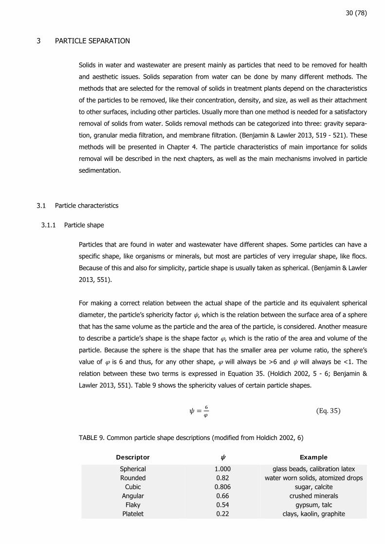
Lawler 2013, 551). Table 9 shows the sphericity values of certain particle shapes.
Eq.35
TABLE 9. Common particle shape descriptions (modified from Holdich 2002, 6)
Descriptor ψ Example
Spherical Rounded
Cubic Angular Flaky
Platelet
1.000 0.82 0.806 0.66 0.54 0.22
glass beads, calibration latex water worn solids, atomized drops
sugar, calcite crushed minerals
gypsum, talc clays, kaolin, graphite
31 (78)
3.1.2 Particle size
Particle size is expressed in terms of diameter, considering that the particle is spherical (Chapter
3.1.1), and its units are expressed in micrometers (µm). Particles in water and wastewater are present
in all sizes between a certain range. Usually the lower limit of this range is set arbitrarily or by the
measuring device’s detection capability. On the other hand, there is always an upper limit that depends
on the physical treatments that the water has received. (Benjamin & Lawler 2013, 546). The particles
present in water and wastewater can be classified as suspended particles or colloidal particles. Colloi-
dal particles are usually in the size range of 0.001 to 1 µm and cannot be separated by sedimentation
processes. (Tchobanoglous et al. 2014, 461 - 462).
There are different methods for measuring the size of the particles in a sample, the most simple being
observation through a microscope, although this method is limited and not very practical. More com-
monly, electronic particle size analyzers are used for this measurement. The measurement in this kind
of analyzers is based either in changes in the conductivity of the sample or in the light intensity
changes of a laser beam. These changes vary with respect to particle size and produce electrical
signals that are sensed by the analyzer, which has to be calibrated beforehand with spheres of differ-
ent and known sizes. Each of these electrical signals is then related to the size of the particle. (Ben-
jamin & Lawler 2013, 550 - 551; Tchobanoglous et al. 2014, 76 - 78).
The number of particles measured between each size range is the particle size distribution of the
sample. Particle size distribution is a function of the diameter and can be presented in terms of num-
ber, area, or volume of the particles, and also differentially or cumulatively. Differential distributions
in a logarithmic scale are most frequently used. Whether to present the number of particles, their
area or their volume in the distribution depends on the particle characteristic that is relevant to the
process. For example, for flocculation, surface area is relevant, whereas for sedimentation, it is the
volume that matters the most. Also, for different processes, the size ranges and their changes can
vary. For example, a decrease in smaller particles in flocculation and a decrease of larger particles in
sedimentation. (Benjamin & Lawler 2013, 548 – 549).
3.1.3 Particle charge
There are three main ways a particle’s surface becomes positively or negatively charged: isomorphic
substitution, chemical reactions, and adsorption. Isomorphic substitution occurs commonly in clays
and it is due to the substitution of certain elements in the crystal arrangements of a solid. If the
substitute element has a different valence than the replaced original element, the net charge of the
solid will change. Chemical reactions at the surface of a particle depend on the water’s pH. These
reactions happen in solids that have acidic or basic functional groups, like oxides, hydroxides, car-
bonates, phosphates, and the carboxyl and amino groups of bacteria, for example. With changes in
pH, these solids can become protonated or deprotonated and, thus, become positively or negatively
32 (78)
charged. Finally, adsorption on the particle surface is caused by the ions present in water and their
interactions with the particles. The adsorption of these ions contributes to the charge of the particle.
(Benjamin & Lawler 2013, 522 - 523).
The charge on the surface of particles helps the particle size distribution to remain the same, in other
words, makes the particles stable. Thus, for an efficient removal of particles from water, usually the
particles have to be destabilized, especially if the particles are colloidal. When two moving particles
are either positively or negatively charged, a rejection force between the two will prevent them from
collision. Nevertheless, despite being equally charged, if the two particles are close enough, the at-
tractive London-van der Waals forces could bring them together. (Benjamin & Lawler 2013, 521).
The London-van der Waals forces originate from the interaction of two molecules and their polariza-
tion. The movement of the electron cloud in a molecule can cause it to be slightly polar at certain
times, even if the molecule is nonpolar. When two molecules approach each other, the position of the
electron cloud with respect of the other molecule can cause an attraction or rejection between the
two of them. For example, if the electron cloud of one molecule faces the positive side of the other
molecule, they will experience an attraction. Usually, attractive forces will be longer and more stable
than rejection forces and will remain until the molecules separate due to their kinetic energy. (Benja-
min & Lawler 2013, 526 -527).
3.1.4 Particle density
The density of particles in water has a wide range, for example, the density of some mineral particles
is between 4 and 5 kg/m3 while flocs and organisms are almost as dense as water. It is the difference
between the density of the particles and the density of water that is of main importance for their
behavior in water and their further separation, especially in gravity separation. (Benjamin & Lawler
2013, 552). Table 10 shows the densities of some particles commonly encountered in water and
wastewater treatment.
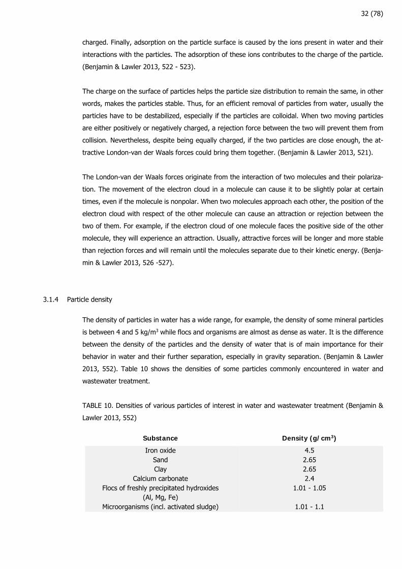
TABLE 10. Densities of various particles of interest in water and wastewater treatment (Benjamin &
Lawler 2013, 552)
Substance Density (g/cm3)
Iron oxide Sand Clay
Calcium carbonate Flocs of freshly precipitated hydroxides
(Al, Mg, Fe) Microorganisms (incl. activated sludge)
4.5 2.65 2.65 2.4
1.01 - 1.05
1.01 - 1.1
33 (78)
3.1.5 Particle destabilization
As noted in Chapters 3.1.2 and 3.1.3, particles that are difficult to settle, like colloids, have to be
destabilized in order to remove them by sedimentation processes. The mechanisms for particle desta-
bilization are mainly four: adsorption and charge neutralization, enmeshment in a precipitate (sweep
flocculation), adsorption and interparticle bridging, and compression of the diffuse layer. (Benjamin &
Lawler 2013, 535).
These mechanisms depend in part on the chemicals (also known as coagulants or flocculants) that
are added to the suspension. The type and amount of chemical to be added depends on the suspen-
sion properties and has to be determined beforehand with tests (called jar tests). The minimum
amount of chemical to destabilize the suspension is known as the critical coagulation concentration
(CCC). (Benjamin & Lawler 2013, 535 – 537).
The most commonly used chemicals for destabilization are aluminum and iron salts, and organic pol-
ymers. Aluminum is added as aluminum sulfate (Al2(SO4)3 · xH2O) and iron is added either as ferric
sulfate (Fe2(SO4)3) or ferric chloride (FeCl3). Hydroxides of these metals precipitate during destabili-
zation. Both metal chemistries are quite similar, with the difference that the pH for minimum solubility
of Al(OH)3 is about 6.5 while Fe(OH)3 is less soluble and its minimum solubility pH is about 8.0, which
makes the latest a more convenient choice in water treatment. The addition of the metal salts reduces
alkalinity and pH, so pH is usually monitored and controlled, as well as alkalinity in low alkalinity
waters, with the addition of a base. (Benjamin & Lawler 2013, 532 – 533).
The organic polymers that are usual in water and wastewater treatment are the positively charged,
low-molecular polydiallyldimethyl ammonium chloride (polyDADMAC) and epichlorohydrin dimethyla-
mine (epi-DMA). The use of these polymers is especially useful in cases where the pH varies quickly
in a wide range because their charge density does not change over a large pH range. Organic polymers
adsorb to particle surfaces, thus, changing particle characteristics and interactions with each other.
(Benjamin & Lawler 2013, 533 - 534).
The mechanism by which aluminum and iron salts, as well as organic polymers act, is the adsorption
and charge neutralization mechanism. Colloidal particles in water and wastewater are usually nega-
tively charged, and that is why these kinds of coagulants are the most common. Other chemicals and
their mechanisms are ferric chloride in sweep flocculation, synthetic (acrylamide based) polymers in
adsorption and interparticle bridging, and inorganic electrolytes (like sodium chloride or calcium chlo-
ride) in compression of the diffuse layer. (Benjamin & Lawler 2013, 535 - 541).
34 (78)
Particle settling
Particles denser than water can settle with the aid of gravity and be, thus, separated by sedimentation
processes (gravity separation). Particle sedimentation, or settling, can occur mainly in four different
ways: discrete settling, flocculent settling, hindered settling and compression settling (RIL II 2003,
78). The different gravity separation methods commonly used in water treatment are presented in
Chapter 4.
3.2.1 Discrete settling
Discrete settling, or Type I sedimentation, occurs in solutions that have low particle concentration and
particles that do not tend to flocculate, so the particles can settle individually without interacting with
any other particles (RIL II 2003, 76).
The particles of the solution settle influenced only by the gravitational force FG and the drag force FD
that originates from the particle motion inside a fluid. The mass of the particle considered in the
calculation of the gravitational force (Eq. 3) is given by the difference between the particle’s and the
water’s density. When both the gravitational and the drag forces are equal, the particle settles at a
steady velocity (Eq. 36).
Eq.36
where v is the settling velocity of the particle, ρp and ρw are the densities of the particle and the water
respectively, V is the volume of the particle, CD is the drag coefficient and Ap is the projected cross-
section area of the particle. Considering the particle a sphere of diameter d, Equation 28 can be
expressed as in Equation 37. (RIL II 2003, 79 - 80; Tchobanoglous et al. 2014, 346 - 348).
Eq.37
The drag coefficient CD of spherical particles in the laminar region can be calculated with Equation 38.
Substitution of CD in Equation 37 results in what is known as Stoke’s law (Eq. 39). (Tchobanoglous et
al. 2014, 347 - 348).
Eq.38
Eq.39
35 (78)
Although the Stoke’s law describes the downwards settling velocity of a particle, if the density of the
particle is less than that of the water, the same expression can be used for describing the particle’s
upwards flotation velocity. Nevertheless, the assumptions made in the Stoke’s law, like the spherical
shape of the particle and the settling in the laminar region, are conditions that rarely occur in water
treatment and, hence, limit its use. (Benjamin & Lawler 2013, 608).
For overcoming these limitations, the value of CD can be calculated as in Equation 40 for settling in
the transitional region and as in Equation 41 for settling in the turbulent region. Also, the shape of
the particle can be considered by multiplying Re by the sphericity ψ value of the particle or multiplying
CD by the particle’s shape factor φ (Chapter 3.1.1). (Tchobanoglous et al 2014, 347 - 348; RIL II
2003, 79 - 81).
√
0.34 Eq.40
0.4 Eq.41
3.2.2 Flocculent settling
In flocculent settling (Type II sedimentation), the solution’s particle concentration is low but, unlike
in discrete settling, the particles in the solution tend to flocculate. The settling velocity of the particles
is no longer constant, because when the particles start to stick together, their size and mass increase
and, thus, also their settling velocity increases. Flocculation will continue throughout the settling tra-
jectory and so the particles will constantly accelerate. For this reason, particles will settle faster than
in discrete settling. (Benjamin & Lawler, 603, 620).
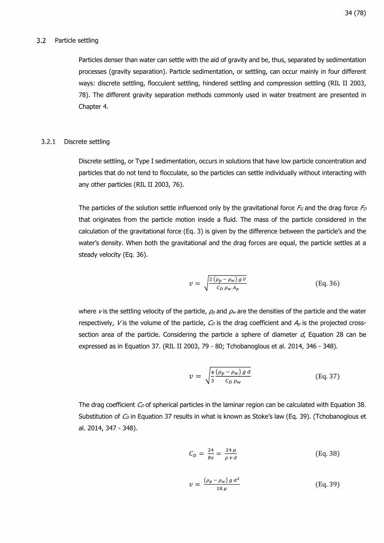
Flocculent settling is strongly influenced by particle concentration, as well as size range and detention
time, among others. For this reason, there is not enough theoretical information to predict the floc-
culation rate or the settling velocity of a certain solution and, therefore, sedimentation tests of the
solution have to be made in the laboratory. The results of these tests are usually represented in terms
of time, depth, and percentage of solids removal (Figure 19). (Tchobanoglous et al. 2014, 354; RIL
II 2003, 82; Droste 1997, 299).
36 (78)
FIGURE 19. Isoconcentration curves (modified from Droste 1997, 302)
3.2.3 Hindered settling
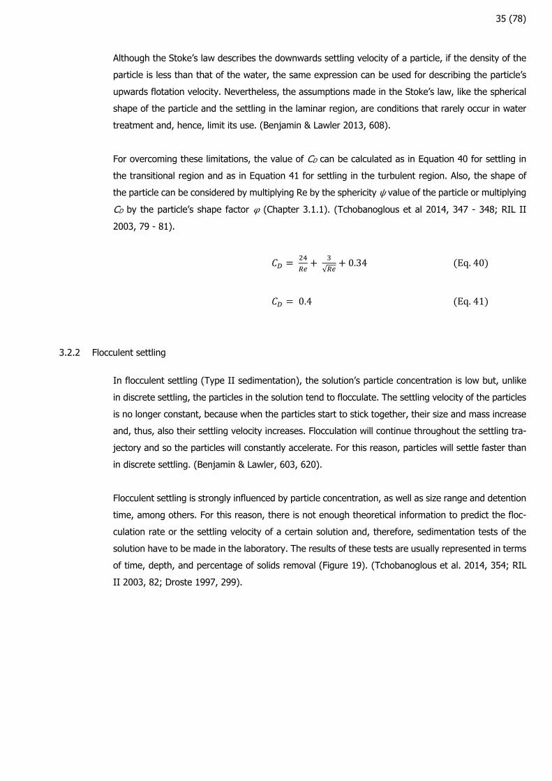
The third type of sedimentation, called hindered or zone settling, occurs in solutions with high solids
concentration. As particles settle, water flows upwards between the particles, causing the particles to
remain in the same position with respect of each other. Because of this, particles continue to settle
as an entity. During sedimentation, a zone of clear liquid starts to form on the top and a settling zone
at the bottom, which is the entity of settling particles. (Tchobanoglous et al. 2014, 360; Droste 1997,
308 - 309).
As time passes, the solids at the bottom start to get closer and compress, creating a compression
zone. Between the compression zone and the hindered zone becomes visible a transition zone, whose
concentration decreases from the compression zone to the hindered zone. Eventually, the solution will
reach what is called the critical point, when both the hindered zone and the transition zone disappear
(Figure 20). (Tchobanoglous et al. 2014, 360 - 361; RIL 2003, 82).
Although the velocity of sedimentation of a solution in this type of settling also has to be tested, in
1952, Kynch assumed that the settling velocity in each zone depends only on the solids concentration
of the zone. From his work is shown that particles in the hindered zone have a constant settling
velocity, which starts to decrease in the transition zone, until they finally reach the compression zone.
Before the hindered zone sometimes can be present an indefinite zone where flocs are formed. Par-
ticles remaining in the clear zone can settle as in discrete or flocculent settling, depending on their
characteristics. (Tchobanoglous et al. 2014, 360 - 361; RIL II 2003, 83).
37 (78)
FIGURE 20. Definition sketch for hindered settling (modified from Tchobanoglous et al. 2014, 360)
3.2.4 Compression settling
Finally, compression settling (Type IV sedimentation) occurs after hindered settling in high concen-
tration solutions (Figure 20). As particles settle, their weight pressures against the bottom layer of
flocs. Because of this compression, the flocs at the bottom get closer together and lose water. Further
compression of this layer can be obtained by stirring, which helps release more water from the flocs.
The characteristics of this kind of settling in a particular solution and the effects of stirring have to be
determined with sedimentation tests in the laboratory. (Tchobanoglous 2014, 360, 364; RIL II 2003,
82 - 84).
38 (78)
4 SOLID SEPARATION METHODS
Screening
Screening is one of the first solids removal processes in water and wastewater treatment, although
for raw water it is not always required and it is mostly needed in water intake from rivers. In this
process, large solids, like trash, paper, leaves and sticks, for example, are separated from the influent
water by passing the water through openings of certain, uniform size. The aim of screening is to
separate solids that could damage the equipment, like pumps, or affect the efficiency of the whole
treatment process. The openings of the screens can have any shape and can be made of bars (bar
racks), mesh or plate perforations. The solid material separated by a screen is called screenings. (RIL
II 2003, 53 - 54; Tchobanoglous et al. 2014, 310).
Screens can be classified as coarse, medium, and fine screens, depending on the size of their open-
ings. The smaller the size of the openings of the screen is, the more the amount of screenings and
need of cleaning. The opening size range for each type is about 40 to 100 mm for coarse screens, 10
to 40 mm for medium screens, and <10 mm for fine screens. In addition to these, there are fine
strainers and microscreens with an opening size of about 0.5 to 6 mm for the first and <0.5 mm for
the latter. However, these may be used in a different part of the treatment process and may replace
other sedimentation processes, since they can also separate some percentage of suspended solids.
(RIL II 2003, 53, 502; Tchobanoglous et al. 2014, 310 - 311, 323).
In the design or installation of screens, it is important to consider some aspects, like location, inclina-
tion, head loss, opening size, velocity, and screenings disposal, among others. Inclination is usually
between 30 to 60 degrees and is important especially in the means of cleaning of the screen, which
can be done manually or mechanically. The velocity of the water flow in screening should be over 0.4
m/s but less than 1 m/s. With a lower velocity, the solids could settle before the screen but, with a
high velocity, the solids could squeeze through the openings. (Tchobanoglous et al. 2014, 316; RIL II
2003, 53; Droste 1997, 287).
Sedimentation
Sedimentation is a settleable suspended solids removal process that usually comes as the first process
in water and wastewater treatment facilities after grit and coarse solids removal (like screening),
although it can also be used as a secondary treatment process after biological treatment. In this
process, settleable solids are let to settle in tanks of circular or rectangular shape, known as clarifiers
or sedimentation basins, and are then removed by scraping. Floating material (scum) can be removed
by skimming of the surface. (Tchobanoglous et al. 2014, 17, 382 - 383).
One of the main parameters for designing a clarifier is to determine its surface loading rate. A rectan-
gular tank of length l, width b, and depth h with a steady flow rate Q, has a flow velocity equal to:
39 (78)
Eq.42
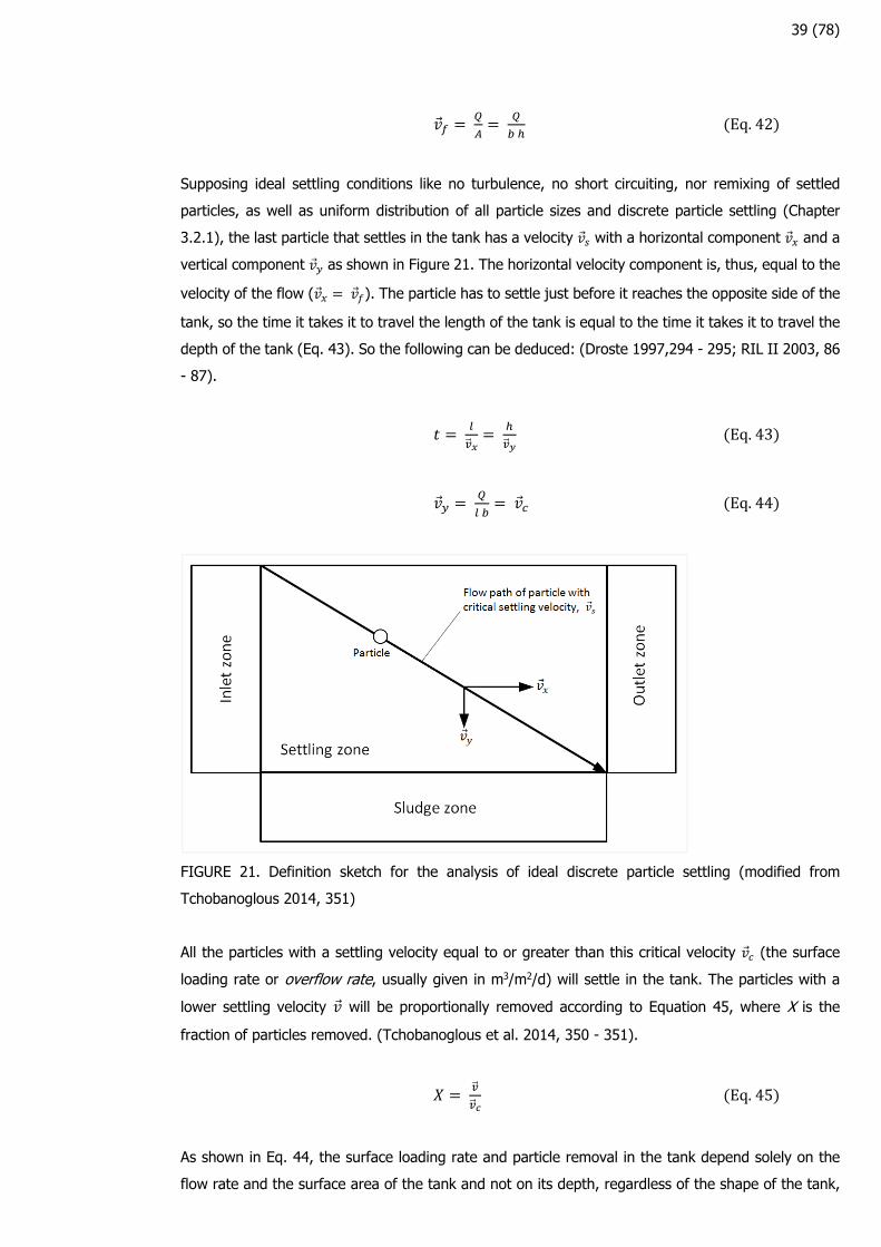
Supposing ideal settling conditions like no turbulence, no short circuiting, nor remixing of settled
particles, as well as uniform distribution of all particle sizes and discrete particle settling (Chapter
3.2.1), the last particle that settles in the tank has a velocity with a horizontal component and a
vertical component as shown in Figure 21. The horizontal velocity component is, thus, equal to the
velocity of the flow ( ). The particle has to settle just before it reaches the opposite side of the
tank, so the time it takes it to travel the length of the tank is equal to the time it takes it to travel the
depth of the tank (Eq. 43). So the following can be deduced: (Droste 1997,294 - 295; RIL II 2003, 86
- 87).
Eq.43
Eq.44
FIGURE 21. Definition sketch for the analysis of ideal discrete particle settling (modified from
Tchobanoglous 2014, 351)
All the particles with a settling velocity equal to or greater than this critical velocity (the surface
loading rate or overflow rate, usually given in m3/m2/d) will settle in the tank. The particles with a
lower settling velocity will be proportionally removed according to Equation 45, where X is the
fraction of particles removed. (Tchobanoglous et al. 2014, 350 - 351).
Eq.45
As shown in Eq. 44, the surface loading rate and particle removal in the tank depend solely on the
flow rate and the surface area of the tank and not on its depth, regardless of the shape of the tank,
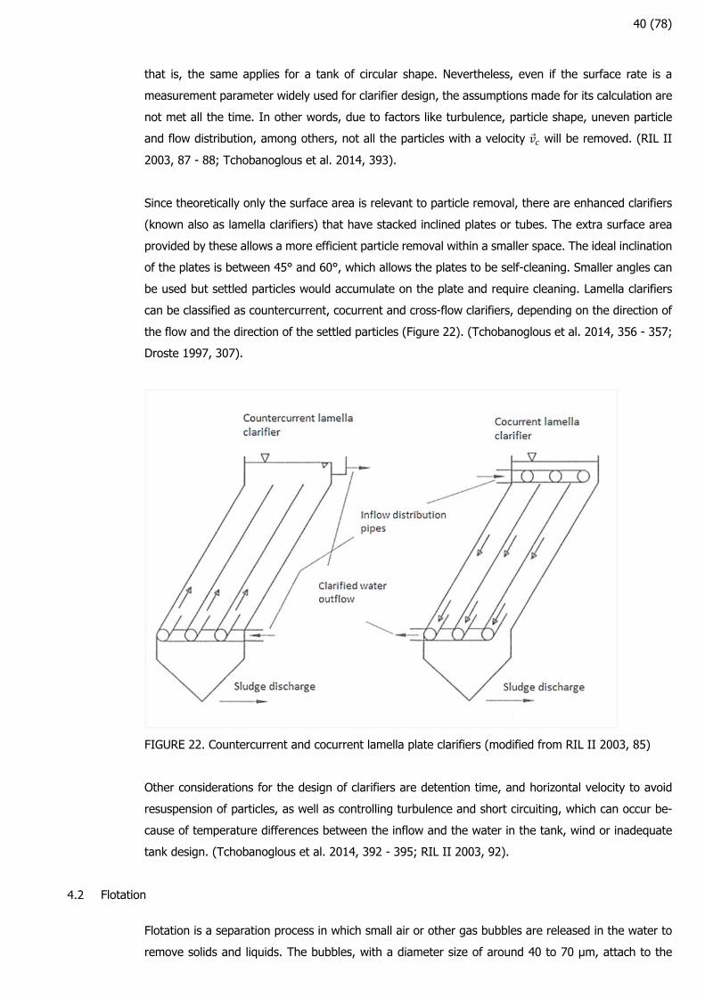
40 (78)
that is, the same applies for a tank of circular shape. Nevertheless, even if the surface rate is a
measurement parameter widely used for clarifier design, the assumptions made for its calculation are
not met all the time. In other words, due to factors like turbulence, particle shape, uneven particle
and flow distribution, among others, not all the particles with a velocity will be removed. (RIL II
2003, 87 - 88; Tchobanoglous et al. 2014, 393).
Since theoretically only the surface area is relevant to particle removal, there are enhanced clarifiers
(known also as lamella clarifiers) that have stacked inclined plates or tubes. The extra surface area
provided by these allows a more efficient particle removal within a smaller space. The ideal inclination
of the plates is between 45° and 60°, which allows the plates to be self-cleaning. Smaller angles can
be used but settled particles would accumulate on the plate and require cleaning. Lamella clarifiers
can be classified as countercurrent, cocurrent and cross-flow clarifiers, depending on the direction of
the flow and the direction of the settled particles (Figure 22). (Tchobanoglous et al. 2014, 356 - 357;
Droste 1997, 307).
FIGURE 22. Countercurrent and cocurrent lamella plate clarifiers (modified from RIL II 2003, 85)
Other considerations for the design of clarifiers are detention time, and horizontal velocity to avoid
resuspension of particles, as well as controlling turbulence and short circuiting, which can occur be-
cause of temperature differences between the inflow and the water in the tank, wind or inadequate
tank design. (Tchobanoglous et al. 2014, 392 - 395; RIL II 2003, 92).
Flotation
Flotation is a separation process in which small air or other gas bubbles are released in the water to
remove solids and liquids. The bubbles, with a diameter size of around 40 to 70 µm, attach to the
41 (78)
surface of the particles (or flocs of particles) increasing their buoyancy and making them float, even
if the particles are denser than water. The floating particles are then removed by skimming of the
surface of the water. The rise of particles less dense than water, like oil and grease, is also known as
natural flotation, although air flotation can be used to make them rise faster. Destabilization of the
particles by coagulation (Chapter 3.1.5) is also used along with this process to improve the attachment
of the bubbles to the particles. (RIL II 2003 97; Tchobanoglous et al. 2014, 403 - 406).
There are two main processes by which the bubbles in the water are formed. One way is to make the
water become supersaturated with air by saturating it under pressure and then releasing the pressure
to atmospheric level. This process is known as dissolved-air flotation (DAF) and it is the mostly used
in municipal wastewater treatment facilities. However, is not always convenient to pressurize all the
incoming flow, especially in large facilities, so it is only part of the treated water that is returned to
the process, pressurized, and saturated with air. The second way is to mix the air into the water at
atmospheric pressure with a rotating impeller, which is known as dispersed-air or induced-air flotation.
This process is used mostly for removal of oils and suspended solids of industrial wastewaters.
(Tchobanoglous et al. 2014, 404 - 405).
For the design of DAF systems, one of the most important parameters to determine is the volume of
air and mass of solids ratio (A/S). This parameter is a function of the solubility of air, the operating
pressure and the solids concentration and it is obtained experimentally with laboratory tests of the
actual solution to be treated. Other parameters that affect the clarification process are the solids
loading rate and the rise velocity of the particles. (Tchobanoglous et al. 2014, 406 - 407).
Filtration
Filtration is a process by which small suspended or colloidal particles are removed from water, which
is why filtration is often used as a complement after sedimentation or flotation (Droste 1997, 229).
Filtration can be divided as depth filtration or surface filtration. In the first one, filtration occurs by
passing the suspension through a whole layer of granular media, while in the latest, the solution is
passed through a thin, porous material. A third type of filtration is membrane filtration, which differs
from surface filtration by the size of the openings of the filter material, which are 5 – 30 µm for surface
filtration and <2 µm for membrane filtration. (Tchobanoglous et al. 2014, 1129, 1171).
Surface filtration can be used instead of granular filtration to remove suspended solids and algae or
as a pretreatment before membrane filtration. The filters in this type of filtration have openings of 5
to 30 µm and can be classified as two-dimensional (synthetic or woven metal fabrics) or three-dimen-
sional (like polyester needle felt cloth). Most commonly, surface filtration is accomplished by several
rotating metal disks on which the filter material is attached. (Tchobanoglous et al. 2014, 1171 - 1175).
On the other hand, membrane filtration can be furtherly classified as microfiltration, ultrafiltration,
nanofiltration, reverse osmosis, and electrodialysis, depending on the size of the pores of the filter
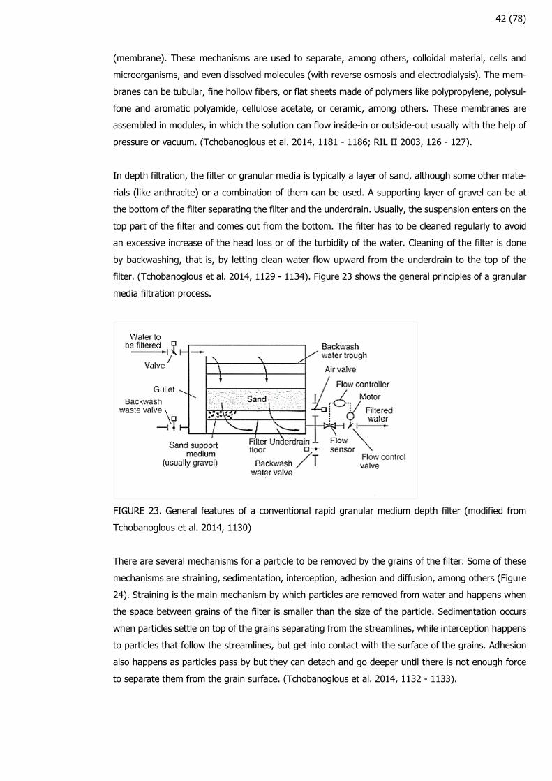
42 (78)
(membrane). These mechanisms are used to separate, among others, colloidal material, cells and
microorganisms, and even dissolved molecules (with reverse osmosis and electrodialysis). The mem-
branes can be tubular, fine hollow fibers, or flat sheets made of polymers like polypropylene, polysul-
fone and aromatic polyamide, cellulose acetate, or ceramic, among others. These membranes are
assembled in modules, in which the solution can flow inside-in or outside-out usually with the help of
pressure or vacuum. (Tchobanoglous et al. 2014, 1181 - 1186; RIL II 2003, 126 - 127).
In depth filtration, the filter or granular media is typically a layer of sand, although some other mate-
rials (like anthracite) or a combination of them can be used. A supporting layer of gravel can be at
the bottom of the filter separating the filter and the underdrain. Usually, the suspension enters on the
top part of the filter and comes out from the bottom. The filter has to be cleaned regularly to avoid
an excessive increase of the head loss or of the turbidity of the water. Cleaning of the filter is done
by backwashing, that is, by letting clean water flow upward from the underdrain to the top of the
filter. (Tchobanoglous et al. 2014, 1129 - 1134). Figure 23 shows the general principles of a granular
media filtration process.
FIGURE 23. General features of a conventional rapid granular medium depth filter (modified from
Tchobanoglous et al. 2014, 1130)
There are several mechanisms for a particle to be removed by the grains of the filter. Some of these
mechanisms are straining, sedimentation, interception, adhesion and diffusion, among others (Figure
24). Straining is the main mechanism by which particles are removed from water and happens when
the space between grains of the filter is smaller than the size of the particle. Sedimentation occurs
when particles settle on top of the grains separating from the streamlines, while interception happens
to particles that follow the streamlines, but get into contact with the surface of the grains. Adhesion
also happens as particles pass by but they can detach and go deeper until there is not enough force
to separate them from the grain surface. (Tchobanoglous et al. 2014, 1132 - 1133).
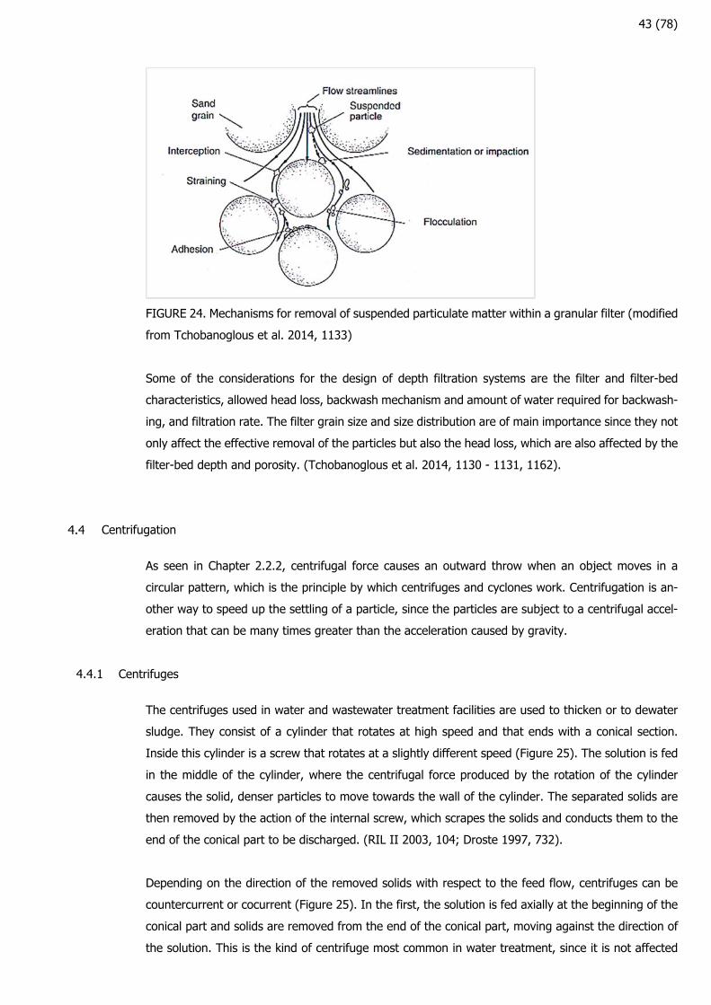
43 (78)
FIGURE 24. Mechanisms for removal of suspended particulate matter within a granular filter (modified
from Tchobanoglous et al. 2014, 1133)
Some of the considerations for the design of depth filtration systems are the filter and filter-bed
characteristics, allowed head loss, backwash mechanism and amount of water required for backwash-
ing, and filtration rate. The filter grain size and size distribution are of main importance since they not
only affect the effective removal of the particles but also the head loss, which are also affected by the
filter-bed depth and porosity. (Tchobanoglous et al. 2014, 1130 - 1131, 1162).
Centrifugation
As seen in Chapter 2.2.2, centrifugal force causes an outward throw when an object moves in a
circular pattern, which is the principle by which centrifuges and cyclones work. Centrifugation is an-
other way to speed up the settling of a particle, since the particles are subject to a centrifugal accel-
eration that can be many times greater than the acceleration caused by gravity.
4.4.1 Centrifuges
The centrifuges used in water and wastewater treatment facilities are used to thicken or to dewater
sludge. They consist of a cylinder that rotates at high speed and that ends with a conical section.
Inside this cylinder is a screw that rotates at a slightly different speed (Figure 25). The solution is fed
in the middle of the cylinder, where the centrifugal force produced by the rotation of the cylinder
causes the solid, denser particles to move towards the wall of the cylinder. The separated solids are
then removed by the action of the internal screw, which scrapes the solids and conducts them to the
end of the conical part to be discharged. (RIL II 2003, 104; Droste 1997, 732).
Depending on the direction of the removed solids with respect to the feed flow, centrifuges can be
countercurrent or cocurrent (Figure 25). In the first, the solution is fed axially at the beginning of the
conical part and solids are removed from the end of the conical part, moving against the direction of
the solution. This is the kind of centrifuge most common in water treatment, since it is not affected
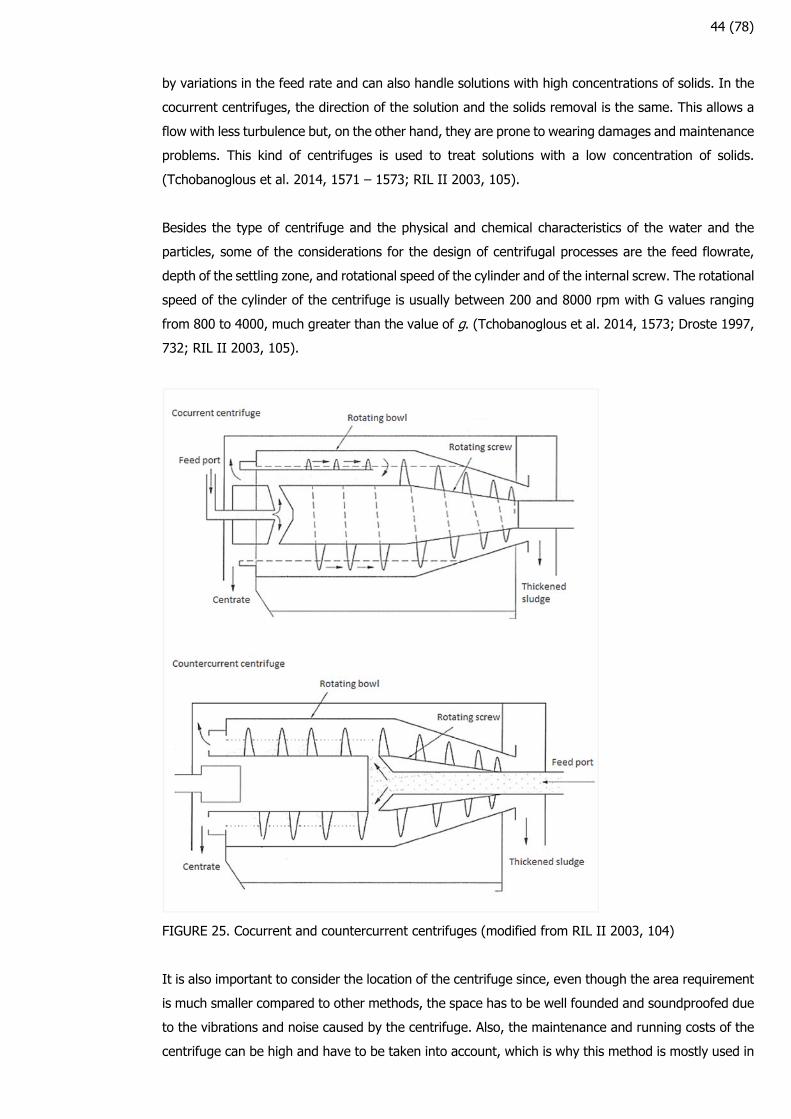
44 (78)
by variations in the feed rate and can also handle solutions with high concentrations of solids. In the
cocurrent centrifuges, the direction of the solution and the solids removal is the same. This allows a
flow with less turbulence but, on the other hand, they are prone to wearing damages and maintenance
problems. This kind of centrifuges is used to treat solutions with a low concentration of solids.
(Tchobanoglous et al. 2014, 1571 – 1573; RIL II 2003, 105).
Besides the type of centrifuge and the physical and chemical characteristics of the water and the
particles, some of the considerations for the design of centrifugal processes are the feed flowrate,
depth of the settling zone, and rotational speed of the cylinder and of the internal screw. The rotational
speed of the cylinder of the centrifuge is usually between 200 and 8000 rpm with G values ranging
from 800 to 4000, much greater than the value of g. (Tchobanoglous et al. 2014, 1573; Droste 1997,
732; RIL II 2003, 105).
FIGURE 25. Cocurrent and countercurrent centrifuges (modified from RIL II 2003, 104)
It is also important to consider the location of the centrifuge since, even though the area requirement
is much smaller compared to other methods, the space has to be well founded and soundproofed due
to the vibrations and noise caused by the centrifuge. Also, the maintenance and running costs of the
centrifuge can be high and have to be taken into account, which is why this method is mostly used in
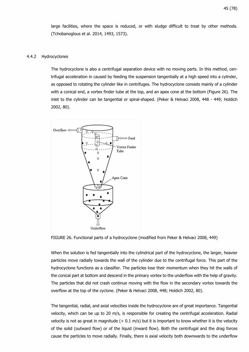
45 (78)
large facilities, where the space is reduced, or with sludge difficult to treat by other methods.
(Tchobanoglous et al. 2014, 1493, 1573).
4.4.2 Hydrocyclones
The hydrocyclone is also a centrifugal separation device with no moving parts. In this method, cen-
trifugal acceleration in caused by feeding the suspension tangentially at a high speed into a cylinder,
as opposed to rotating the cylinder like in centrifuges. The hydrocyclone consists mainly of a cylinder
with a conical end, a vortex finder tube at the top, and an apex cone at the bottom (Figure 26). The
inlet to the cylinder can be tangential or spiral-shaped. (Peker & Helvaci 2008, 448 - 449; Holdich
2002, 80).
FIGURE 26. Functional parts of a hydrocyclone (modified from Peker & Helvaci 2008, 449)
When the solution is fed tangentially into the cylindrical part of the hydrocyclone, the larger, heavier
particles move radially towards the wall of the cylinder due to the centrifugal force. This part of the
hydrocyclone functions as a classifier. The particles lose their momentum when they hit the walls of
the conical part at bottom and descend in the primary vortex to the underflow with the help of gravity.
The particles that did not crash continue moving with the flow in the secondary vortex towards the
overflow at the top of the cyclone. (Peker & Helvaci 2008, 448; Holdich 2002, 80).
The tangential, radial, and axial velocities inside the hydrocyclone are of great importance. Tangential
velocity, which can be up to 20 m/s, is responsible for creating the centrifugal acceleration. Radial
velocity is not as great in magnitude (< 0.1 m/s) but it is important to know whether it is the velocity
of the solid (outward flow) or of the liquid (inward flow). Both the centrifugal and the drag forces
cause the particles to move radially. Finally, there is axial velocity both downwards to the underflow
46 (78)
with the larger particles and upwards to the overflow with the lighter particles. (Holdich 2002, 80 -
81).
Axial velocity is important to the definition of the cut size (x50) of the hydrocyclone. Since there is axial
velocity downwards and also upwards, there must be a region at a certain radial distance where there
is no axial velocity. The particles that move within this region have the same chance to go to the
underflow or to the overflow and their size is known as the cut size of the hydrocyclone. Most of the
particles that are larger than the cut size will leave in the underflow, while most of the particles smaller
than the cut size will leave in the overflow. The proportion of larger particles that report to the overflow
and of the smaller particles that report to the underflow is given by the grade efficiency and reduced
grade efficiency curves, calculated with Equation 46 and 47. (Holdich 2002, 80 - 83).
Eq.46
Eq.47
where E is the grade efficiency of the hydrocyclone, is the mass flow in size grade in underflow,
is the mass flow size grade in feed, E’ is the reduced grade efficiency, and Rf is the volumetric flow
speed or recovery, which is the relation of volumetric flow in the underflow and the feed.
The separation efficiency of the hydrocyclone is a function of its dimensions, the pressure drop, and
the characteristics of the solution. Factors that reduce separation efficiency include the turbulence of
the flow, short circuiting from the feed to the vortex finder, and mixing in the apex cone area. (Peker
& Helvaci 2008, 450, 456).
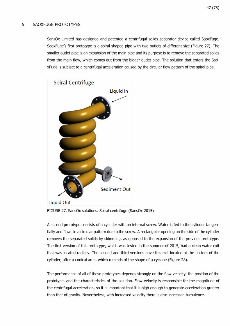
47 (78)
5 SAOXFUGE PROTOTYPES
SansOx Limited has designed and patented a centrifugal solids separator device called SaoxFuge.
SaoxFuge’s first prototype is a spiral-shaped pipe with two outlets of different size (Figure 27). The
smaller outlet pipe is an expansion of the main pipe and its purpose is to remove the separated solids
from the main flow, which comes out from the bigger outlet pipe. The solution that enters the Sao-
xFuge is subject to a centrifugal acceleration caused by the circular flow pattern of the spiral pipe.
FIGURE 27. SansOx solutions. Spiral centrifuge (SansOx 2015)
A second prototype consists of a cylinder with an internal screw. Water is fed to the cylinder tangen-
tially and flows in a circular pattern due to the screw. A rectangular opening on the side of the cylinder
removes the separated solids by skimming, as opposed to the expansion of the previous prototype.
The first version of this prototype, which was tested in the summer of 2015, had a clean water exit
that was located radially. The second and third versions have this exit located at the bottom of the
cylinder, after a conical area, which reminds of the shape of a cyclone (Figure 28).
The performance of all of these prototypes depends strongly on the flow velocity, the position of the
prototype, and the characteristics of the solution. Flow velocity is responsible for the magnitude of
the centrifugal acceleration, so it is important that it is high enough to generate acceleration greater
than that of gravity. Nevertheless, with increased velocity there is also increased turbulence.
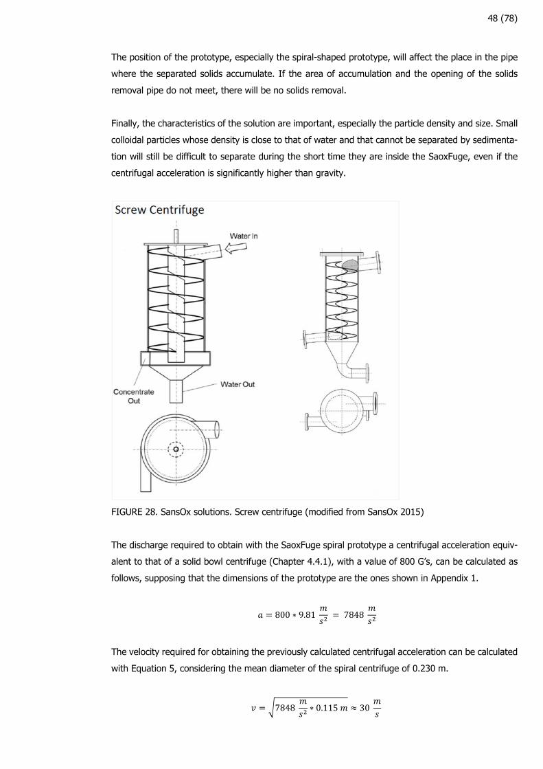
48 (78)
The position of the prototype, especially the spiral-shaped prototype, will affect the place in the pipe
where the separated solids accumulate. If the area of accumulation and the opening of the solids
removal pipe do not meet, there will be no solids removal.
Finally, the characteristics of the solution are important, especially the particle density and size. Small
colloidal particles whose density is close to that of water and that cannot be separated by sedimenta-
tion will still be difficult to separate during the short time they are inside the SaoxFuge, even if the
centrifugal acceleration is significantly higher than gravity.
FIGURE 28. SansOx solutions. Screw centrifuge (modified from SansOx 2015)
The discharge required to obtain with the SaoxFuge spiral prototype a centrifugal acceleration equiv-
alent to that of a solid bowl centrifuge (Chapter 4.4.1), with a value of 800 G’s, can be calculated as
follows, supposing that the dimensions of the prototype are the ones shown in Appendix 1.
800 ∗ 9.81 7848
The velocity required for obtaining the previously calculated centrifugal acceleration can be calculated
with Equation 5, considering the mean diameter of the spiral centrifuge of 0.230 m.
7848 ∗ 0.115 30
49 (78)
The discharge required to obtain this tangential velocity is then calculated by multiplying the velocity
by the cross-sectional area of the pipe. The velocity of the flow has been calculated taking into con-
sideration the lead angle of the spiral, which is approximately 9.4°.
30 ∗ ∗ 0.11032
0.29
The discharge of nearly 300 liters per second makes it quite challenging for the spiral prototype to
generate a centrifugal acceleration slightly similar to that of a solid bowl centrifuge. The challenge is
not only because of the costs of purchasing and especially running the required pump, but also be-
cause of the volume of water needed to be treated, which would be only found in remarkably large
water treatment facilities.
If it would be aimed to avoid the turbulent flow, the velocity needed for the flow to be laminar in the
spiral prototype can be calculated with Equation 13, with a Reynolds number value of 2000.
2000 ∗ 1.518 ∗ 10
1000 ∗ 0.1103 0.028
This velocity equals a flow rate of approximately 0.26 l/s and a centrifugal acceleration of 6.6 * 10-3
m/s2, which is much lower than that of gravity. Thus, the flow cannot be laminar if it is aimed to
generate a centrifugal acceleration that is greater than or even equal to gravity.
Considering the discrete settling of a particle whose density is 2000 kg/m3 and whose diameter is 100
µm in water at 4 °C, the settling velocity of the particle can be calculated with the Stokes law (Equation
36) as follows:
2000 1000 ∗ 9.81 ∗ 10 ∗ 10
18 ∗ 1.518 ∗ 10 0.004
The above mentioned characteristics of the particle and the conditions of the flow were set arbitrarily
but considering a density that is about two times greater than the water density and a size that is big
enough to be considered for removal with sedimentation processes. As mentioned in Chapter 3.2.1,
Stoke’s law considers the particle spherical in shape and the settling occurs in the laminar region.
To increase the settling velocity of this particle ten times with centrifugal force, an acceleration of 10
G’s is needed. To generate this acceleration in the spiral prototype, it would require a discharge of
approximately 33 l/s, as previously calculated. This flow rate, although still large, is more realistic and
accomplishable.
50 (78)
Rounding the discharge value to 30 l/s, which would generate about 8.5 G’s, the Reynolds number
value and the head losses of the flow are calculated.
1000 ∗ 3.14 ∗ 0.1103
1.518 ∗ 10 2.3 ∗ 10
Since the Reynolds number is considerably greater than 4000, the flow is obviously turbulent and
head loss by friction can be calculated using the Darcy-Weisbach equation (Eq. 21) with a friction
factor taken from the Moody diagram using a roughness value k of 0.1 mm (value for a new welded
acid-proof steel pipe from RIL I 2003, 142). The length of the pipe in the spiral has been estimated
using the data in Appendix 1.
0.02 ∗ 4 ∗ 3.14
2 ∗ 9.81 ∗ 0.11030.37
The minor losses in the spiral are caused by the continuous bend of the pipe. Each turn of the spiral
equals four 90° bends, amounting to 20 bends in total. The ratio of the radius of the spiral and the
diameter of the pipe is just about 1, so the resistance coefficient value, taken from Table 7, is 0.40
and the minor losses can be calculated with Equation 26.
20 0.40 ∗3.14
2 ∗ 9.814.0
The total head loss at a flow rate of 30 l/s would be about 4.4 m and it has to be taken into consid-
eration when choosing a pump.
Assuming that settling occurs in the turbulent zone, the particle is not spherical (taking ψ= 0.5), and
the main force acting on the particle is the centrifugal force and not the gravitational force, it is
possible to recalculate the settling velocity of the particle using Equation 36. The drag coefficient in
the turbulent region is calculated by multiplying the value given by Equation 41 by the shape factor
of the particle, calculated with Equation 35.
0.4 ∗ 6
4.8
2 ∗ 2000 1000 ∗ 83.42 ∗ 5.236 ∗ 10
4.8 ∗ 1000 ∗ 7.85 ∗ 10 0.048
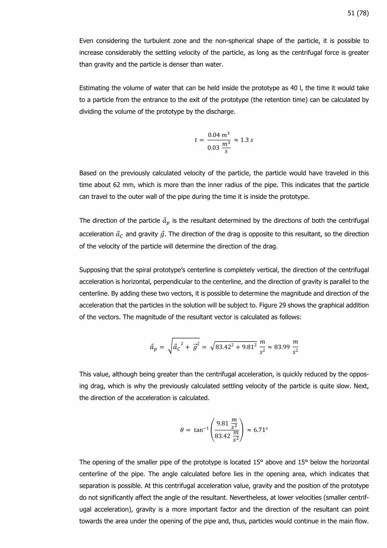
51 (78)
Even considering the turbulent zone and the non-spherical shape of the particle, it is possible to
increase considerably the settling velocity of the particle, as long as the centrifugal force is greater
than gravity and the particle is denser than water.
Estimating the volume of water that can be held inside the prototype as 40 l, the time it would take
to a particle from the entrance to the exit of the prototype (the retention time) can be calculated by
dividing the volume of the prototype by the discharge.
0.04
0.03 1.3
Based on the previously calculated velocity of the particle, the particle would have traveled in this
time about 62 mm, which is more than the inner radius of the pipe. This indicates that the particle
can travel to the outer wall of the pipe during the time it is inside the prototype.
The direction of the particle is the resultant determined by the directions of both the centrifugal
acceleration and gravity . The direction of the drag is opposite to this resultant, so the direction
of the velocity of the particle will determine the direction of the drag.
Supposing that the spiral prototype’s centerline is completely vertical, the direction of the centrifugal
acceleration is horizontal, perpendicular to the centerline, and the direction of gravity is parallel to the
centerline. By adding these two vectors, it is possible to determine the magnitude and direction of the
acceleration that the particles in the solution will be subject to. Figure 29 shows the graphical addition
of the vectors. The magnitude of the resultant vector is calculated as follows:
2
2
83.422 9.812 2 83.99 2
This value, although being greater than the centrifugal acceleration, is quickly reduced by the oppos-
ing drag, which is why the previously calculated settling velocity of the particle is quite slow. Next,
the direction of the acceleration is calculated.
tan9.81
83.42 6.71°
The opening of the smaller pipe of the prototype is located 15° above and 15° below the horizontal
centerline of the pipe. The angle calculated before lies in the opening area, which indicates that
separation is possible. At this centrifugal acceleration value, gravity and the position of the prototype
do not significantly affect the angle of the resultant. Nevertheless, at lower velocities (smaller centrif-
ugal acceleration), gravity is a more important factor and the direction of the resultant can point
towards the area under the opening of the pipe and, thus, particles would continue in the main flow.
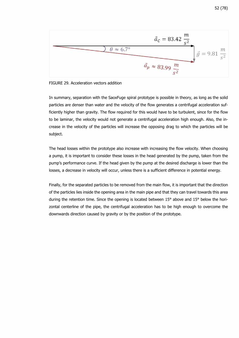
52 (78)
FIGURE 29. Acceleration vectors addition
In summary, separation with the SaoxFuge spiral prototype is possible in theory, as long as the solid
particles are denser than water and the velocity of the flow generates a centrifugal acceleration suf-
ficiently higher than gravity. The flow required for this would have to be turbulent, since for the flow
to be laminar, the velocity would not generate a centrifugal acceleration high enough. Also, the in-
crease in the velocity of the particles will increase the opposing drag to which the particles will be
subject.
The head losses within the prototype also increase with increasing the flow velocity. When choosing
a pump, it is important to consider these losses in the head generated by the pump, taken from the
pump’s performance curve. If the head given by the pump at the desired discharge is lower than the
losses, a decrease in velocity will occur, unless there is a sufficient difference in potential energy.
Finally, for the separated particles to be removed from the main flow, it is important that the direction
of the particles lies inside the opening area in the main pipe and that they can travel towards this area
during the retention time. Since the opening is located between 15° above and 15° below the hori-
zontal centerline of the pipe, the centrifugal acceleration has to be high enough to overcome the
downwards direction caused by gravity or by the position of the prototype.
53 (78)
6 REVIEW OF THE PREVIOUS TESTS OF THE PROTOTYPES
The first tests of the SaoxFuge spiral prototype were made during the summer of 2014. The tests
were joint tests of both the SaoxFuge and SansOx’s OxTube, which is an aeration device. The devices
were tested in four different locations with water of different characteristics in each one. These in-
cluded testing with municipal wastewater, industrial wastewater from Valio’s cheese factory in Lapin-
lahti and Powerflute’s Savon Sellu paperboard mill, a propylene glycol and water mix used as anti-
freeze on the airplanes at Kuopio airport, and, finally, groundwater with a high concentration of iron
and manganese.
The second tests of the spiral prototype and first tests of the screw prototype were carried out in the
summer of 2015 at Yara Finland Siilinjärvi site’s concentration plant, where the main product is apatite,
a source of phosphorus for use in fertilizers. These tests were made as part of the KaivosVV project,
a project aiming to improve the technologies for mine water treatment. This project was coordinated
by the Geological Survey of Finland (GTK) and done in cooperation with Savonia University of Applied
Sciences, the University of Eastern Finland (UEF), and the National Institute for Health and Welfare
(THL). In this thesis, only the SaoxFuge 2015 tests will be reviewed.
The water used for the 2015 tests was the overflow of the apatite clarifier of the concentration plant.
Initially, also the water from the intermediate clarifier at the site was intended to be used in the tests,
but because of technical difficulties only the apatite clarifier overflow was used. The site’s manager
Keränen (2015) gave general information about the clarifiers before the tests. For example that, de-
pending on the quarry, the solids feed to the apatite clarifier was about 110 to 140 tons per hour and
the solids concentration of the overflow fluctuated between 0.1 and 1%, with the target being that
the solids concentration of the overflow is permanently below 0.5%.
Before the tests, a preliminary research of the overflow water characteristics was carried out, in which
sedimentation tests, solids concentration and density determination, and particle size analysis were
done. In the sedimentation tests is was noticed that there was a little amount of solids that would
settle in under a minute, even in a few seconds, giving a settling velocity in the range of 0.03 to 0.003
m/s. Nevertheless, there were also a lot of colloidal solids that would not settle at all, or even some
solids that floated.
The solids concentration determination was made according to the SFS-EN 872:2005 standard. The
solids concentration of the apatite clarifier overflow samples was of 0.4%. The density of the solution
was technically the same as water, which can be explained with the fact that the solids concentration
was quite low and did not affect the density of the solution.
Finally, the particle size analysis was made with PAMAS S4031 analyzer, whose measuring range is
from 1 to 200 µm. The results of this analysis showed that the larger number of particles was between
the size range of 10 to 20 µm or smaller, while the larger volume was given by particles in the size
range of 20 to 40 µm.
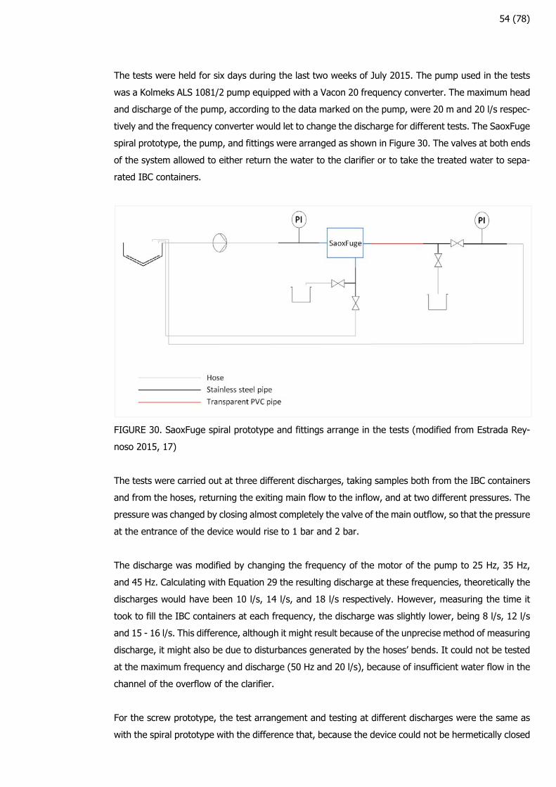
54 (78)
The tests were held for six days during the last two weeks of July 2015. The pump used in the tests
was a Kolmeks ALS 1081/2 pump equipped with a Vacon 20 frequency converter. The maximum head
and discharge of the pump, according to the data marked on the pump, were 20 m and 20 l/s respec-
tively and the frequency converter would let to change the discharge for different tests. The SaoxFuge
spiral prototype, the pump, and fittings were arranged as shown in Figure 30. The valves at both ends
of the system allowed to either return the water to the clarifier or to take the treated water to sepa-
rated IBC containers.
FIGURE 30. SaoxFuge spiral prototype and fittings arrange in the tests (modified from Estrada Rey-
noso 2015, 17)
The tests were carried out at three different discharges, taking samples both from the IBC containers
and from the hoses, returning the exiting main flow to the inflow, and at two different pressures. The
pressure was changed by closing almost completely the valve of the main outflow, so that the pressure
at the entrance of the device would rise to 1 bar and 2 bar.
The discharge was modified by changing the frequency of the motor of the pump to 25 Hz, 35 Hz,
and 45 Hz. Calculating with Equation 29 the resulting discharge at these frequencies, theoretically the
discharges would have been 10 l/s, 14 l/s, and 18 l/s respectively. However, measuring the time it
took to fill the IBC containers at each frequency, the discharge was slightly lower, being 8 l/s, 12 l/s
and 15 - 16 l/s. This difference, although it might result because of the unprecise method of measuring
discharge, it might also be due to disturbances generated by the hoses’ bends. It could not be tested
at the maximum frequency and discharge (50 Hz and 20 l/s), because of insufficient water flow in the
channel of the overflow of the clarifier.
For the screw prototype, the test arrangement and testing at different discharges were the same as
with the spiral prototype with the difference that, because the device could not be hermetically closed
55 (78)
and there was leakage from the lid, tests were carried out only a couple of times at a frequency of 15
Hz, 25 Hz, and 35 Hz.
Samples of both outflow pipes and of the clarifier overflow were taken during each test. The solids
concentration determination and particle size analysis of each sample was made in the laboratory like
it was done in the preliminary research.
If there had been solids separation in the prototypes, the solids concentration in the outflow of the
smaller pipe would have been greater than the one from the main outflow. However, the results of
the tests were inconclusive. While there was a slight difference in a few tests, for example, over
double solids concentration in the smaller pipe outflow in one of the tests at a 25 Hz, for other fre-
quencies and in other tests also at 25 Hz there would be very small difference (of about 0.01 to 0.1%)
or even a lower solids concentration in the smaller pipe outflow. Also the solids concentration results
given by the standard or by the particle analyzer would show differences between them. None of the
discharges or test arrangements would clearly indicate solids separation.
There may be a few reasons for these results. The mixing effect of the turbulent flow could be one of
the reasons. Nevertheless, since the solids were completely mixed before passing through the device,
the solids concentration in both outflows would be the same in every test if the solids continued to be
mixed by turbulence. The differences between the solids concentration results between the standard
and the particle analyzer are caused by the fact that the standard determines solids concentration by
mass, while the particle analyzer determines it by volume. Other reasons would be not enough cen-
trifugal acceleration or retention time to separate the particles, the settling velocities of the particles,
or the angle of accumulation not meeting the expansion of the pipe for removal.
Calculating as in Chapter 5 the conditions of the flow at each frequency (with the discharge and head
given by Equations 29 and 30), as well as the settling velocities of the particles, it is possible to
compare the theoretical conditions of the tests. The results of these calculations are presented in
Table 11.
For the calculation of the velocities of the particles, the diameter of the particles was taken as 30 µm,
which is the average of the size range that predominated in volume (20 – 40 µm), and their density
as the density of apatite, which is of about 3000 kg/m3 (Geologinen tutkimuslaitos 1982, 18). The
shape of the particles is considered spherical, since the particle analyzer results are given according
to the characteristics of a spherical particle.
Other things considered in the calculations were that the temperature of the water was 10 °C, and
the head loss between the pump and the device was given, in addition to the 90° bends of the device,
by the friction loss of the 9 m long lay-flat PVC hose (with a friction loss taken from Kuriyama of
America, Inc. 2013, 15) and also by the sudden contractions and expansions caused by the bends of
the hose (with a resistance coefficient taken from RIL I 2003, 154).
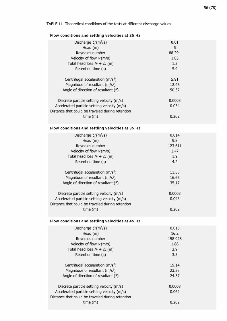
56 (78)
TABLE 11. Theoretical conditions of the tests at different discharge values
Flow conditions and settling velocities at 25 Hz
Discharge Q (m3/s) Head (m)
Reynolds number Velocity of flow v (m/s)
Total head loss hF + hL (m) Retention time (s)
Centrifugal acceleration (m/s2) Magnitude of resultant (m/s2)
Angle of direction of resultant (°)
Discrete particle settling velocity (m/s) Accelerated particle settling velocity (m/s)
Distance that could be traveled during retention time (m)
0.01 5
88 294
1.05 1.2 5.9
5.91 12.46 50.37
0.0008 0.034
0.202
Flow conditions and settling velocities at 35 Hz
Discharge Q (m3/s) Head (m)
Reynolds number Velocity of flow v (m/s)
Total head loss hF + hL (m) Retention time (s)
Centrifugal acceleration (m/s2) Magnitude of resultant (m/s2)
Angle of direction of resultant (°)
Discrete particle settling velocity (m/s) Accelerated particle settling velocity (m/s)
Distance that could be traveled during retention time (m)
0.014 9.8
123 611 1.47 1.9 4.2
11.58 16.66 35.17
0.0008 0.048
0.202
Flow conditions and settling velocities at 45 Hz
Discharge Q (m3/s) Head (m)
Reynolds number Velocity of flow v (m/s)
Total head loss hF + hL (m) Retention time (s)
Centrifugal acceleration (m/s2) Magnitude of resultant (m/s2)
Angle of direction of resultant (°)
Discrete particle settling velocity (m/s) Accelerated particle settling velocity (m/s)
Distance that could be traveled during retention time (m)
0.018 16.2
158 928 1.88 2.9 3.3
19.14 23.25 24.37
0.0008 0.062
0.202
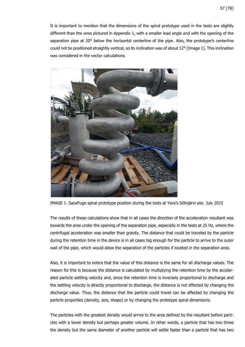
57 (78)
It is important to mention that the dimensions of the spiral prototype used in the tests are slightly
different than the ones pictured in Appendix 1, with a smaller lead angle and with the opening of the
separation pipe at 20° below the horizontal centerline of the pipe. Also, the prototype’s centerline
could not be positioned straightly vertical, so its inclination was of about 12° (Image 1). This inclination
was considered in the vector calculations.
IMAGE 1. SaoxFuge spiral prototype position during the tests at Yara’s Siilinjärvi site. July 2015
The results of these calculations show that in all cases the direction of the acceleration resultant was
towards the area under the opening of the separation pipe, especially in the tests at 25 Hz, where the
centrifugal acceleration was smaller than gravity. The distance that could be traveled by the particle
during the retention time in the device is in all cases big enough for the particle to arrive to the outer
wall of the pipe, which would allow the separation of the particles if located in the separation area.
Also, it is important to notice that the value of this distance is the same for all discharge values. The
reason for this is because the distance is calculated by multiplying the retention time by the acceler-
ated particle settling velocity and, since the retention time is inversely proportional to discharge and
the settling velocity is directly proportional to discharge, the distance is not affected by changing the
discharge value. Thus, the distance that the particle could travel can be affected by changing the
particle properties (density, size, shape) or by changing the prototype spiral dimensions.
The particles with the greatest density would arrive to the area defined by the resultant before parti-
cles with a lower density but perhaps greater volume. In other words, a particle that has two times
the density but the same diameter of another particle will settle faster than a particle that has two
58 (78)
times the diameter but the same density of another particle. If the heavier but smaller particles con-
tinued in the main flow due to the resultant’s direction and the bigger but lighter particles accumulated
in a higher area that could be separated from the main flow, this could explain why in some tests the
smaller pipe outflow had higher solids concentration with the particle analyzer and lower concentration
with the determination by the standard.
Considering the head given by the pump, even at a frequency of 25 Hz, the head loss due to friction
and bends is not that great, theoretically, that it would affect the discharge and explain the difference
between the measured and the theoretical discharge.
From all of this it is possible to deduce that, the inconclusive results of the 2015 tests at Yara’s
Siilinjärvi site might be caused in great part by the insufficient discharge at which the tests were done.
This could cause a centrifugal acceleration that is not high enough to overcome the downwards di-
rection of gravity and to accelerate the particles in the direction towards the separation opening of
the device. In the future, this can be prevented by choosing a more accurate pump for the tests, as
well as by measuring the discharge more precisely with a flow meter located just before the device.
Another reason for the results of the tests might be the particle characteristics of the solids in the
solution. Even if the size range of the particles could be known, in the calculations it was assumed
that the particles had the density of apatite. However, the particle density was not known and the
particles of the overflow of the apatite clarifier could have been of any other material that could be
found in the concentration process, perhaps having a lower density than apatite. The characteristics
of the particles in the solution would have to be known beforehand so that the theoretical data would
be more accurate and the tests of the prototype would be more precise.
Finally, it is appropriate to consider still the probability of mixing due to the turbulent flow and Dean
vortices. Some ways to study this are, for example, to have a transparent prototype that would allow
observing the areas where mixing and possible vortices occur inside the device, as well as with a
deeper theoretical and empirical research with the use of computational fluid dynamics or tomographic
analysis of the particles in the device.
59 (78)
7 LABORATORY-SCALE PROTOTYPE DEVELOPMENT
The conclusions made in Chapters 5 and 6 show the need for further testing and development of the
SaoxFuge. For a better understanding of the separation efficiency that can be achieved with the
SaoxFuge, it is essential to have more control over the variables in the testing of the prototype as well
as to identify what are the parameters that affect the separation process the most.
The size of the prototype used in the previous tests required a large discharge and, thus, a large
amount of water available to do the testing, which limited the testing location. In other words, the
places where the prototype was tested were selected based mainly on their available volume of water
and less on the characteristics of the solids in those waters compared to the characteristics of the
prototype. Another important factor is the variations in the characteristics of those waters (like solids
concentration), which can vary over time and affect also the testing results.
It is because of these reasons that it is suggested testing with a smaller prototype in a laboratory
scale. In the laboratory-scale testing the characteristics of the solution to be treated can be more
easily known or even artificially made (for example adding a certain amount of particles of known
size, density, and shape to water) and, with a smaller prototype, higher centrifugal acceleration can
be achieved with a lower discharge. Also sampling of the inflow and both outflows can be more
manageable compared to the sampling done from the lay-flat hoses or the IBC containers, and particle
size analysis can be achieved inline or online as well.
Based on the calculations made in the previous chapters, an Excel workbook containing the relevant
parameters of the calculations was created in order to visualize how each of the parameters affect
the results related to the theoretical particle separation. By trying different values of prototype dimen-
sions, particle characteristics, and discharges, it was aimed to find the most suitable ranges of proto-
type size as well as types of particles for solids separation testing in a certain prototype. Details of
this Excel workbook are presented in Appendix 2.
Firstly, for finding these ranges, it was considered that the prototype size has to be changed with
respect to the characteristics of the water that has to be treated since the characteristics of the water
are particular of each place of origin, so the first step was to gather general data of the particles
commonly encountered in water and wastewater treatment facilities. Industrial wastewater was lim-
itedly considered, because the characteristics of the particles in these waters depend on the specific
industry from where they come. Besides, the characteristics of the wastewater of a single factory can
also vary depending on its production.
According to Tchobanoglous et al. (2014, 1457), the solids in the primary sedimentation sludge have
a relative density of about 1.4. For the calculations, also the densities of sand, clay, flocs, and micro-
organisms were taken from Table 10 in Chapter 3.1.4. The size of the particles was assumed to be
between 30 and 1000 µm, which is the size range in which sedimentation is typically considered
appropriate. Particles in this size range are, for example, settleable solids, silt particles and some

60 (78)
microbial particles, like bacterial flocs, algae, protozoa, and worms, among others. The density of the
settleable solids was taken as 1200 kg/m3. (Tchobanoglous et al. 2014, 77; RIL II 2003, 106, 508).
Three sizes of prototype were compared to find the minimum density that a spherical particle of
certain diameter has to have in order to be separated in each prototype. This was made by considering
the distance that the particle could travel during the retention time and assuming there is no mixing
due to turbulence or vortices. It is good to notice that, even if both the spiral diameter and the pitch
affect the retention time, adding turns to the spiral is more effective for increasing the retention time,
so smaller particles have more time to travel to the outer wall of the spiral’s pipe.
The dimensions of the biggest prototype were the ones presented in Appendix 1. The sizing of the
other prototypes was made by changing the pipe diameter but keeping the relation between the pipe
diameter and the dimensions of the spiral somehow similar. The number of turns and the angle of the
opening of the separation pipe remained the same for all sizes. Table 12 shows the pipe and spiral
dimensions of each prototype used in the calculations as well as the minimum discharge required for
the direction of the resultant to be within the opening of the separation pipe.
TABLE 12. Dimensions of the prototypes used in the calculations
Prototype DN100
Pipe outer diameter (mm) Pipe inner diameter (mm)
Spiral mean diameter (mm) Pitch (mm)
Number of turns Lead angle (°)
Minimum discharge required (m3/s)
114,3 110,3 230 120 5
9,4 0,020
Prototype DN80
Pipe outer diameter (mm) Pipe inner diameter (mm)
Spiral mean diameter (mm) Pitch (mm)
Number of turns Lead angle (°)
Minimum discharge required (m3/s)
88,9 84,9 180 95 5
9,5 0,011
Prototype DN50
Pipe outer diameter (mm) Pipe inner diameter (mm)
Spiral mean diameter (mm) Pitch (mm)
Number of turns Lead angle (°)
Minimum discharge required (m3/s)
60,3 56,3 122 65 5
9,6 0,004
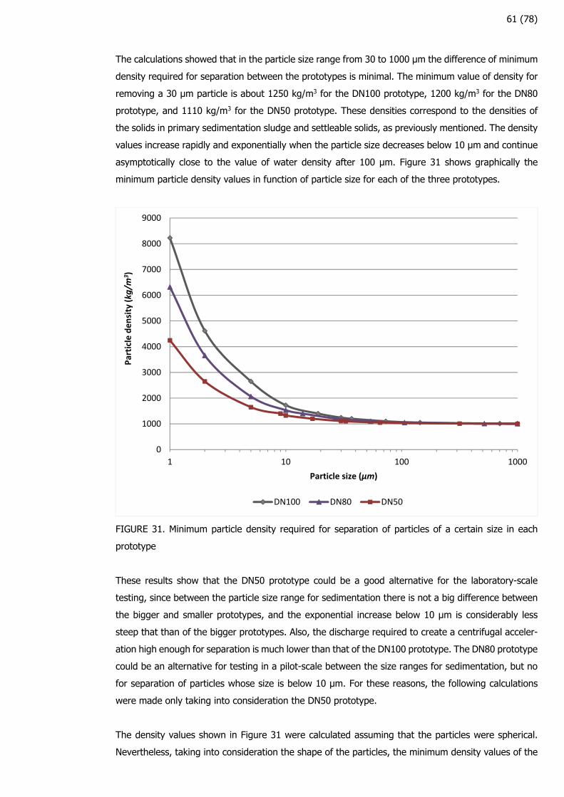
61 (78)
The calculations showed that in the particle size range from 30 to 1000 µm the difference of minimum
density required for separation between the prototypes is minimal. The minimum value of density for
removing a 30 µm particle is about 1250 kg/m3 for the DN100 prototype, 1200 kg/m3 for the DN80
prototype, and 1110 kg/m3 for the DN50 prototype. These densities correspond to the densities of
the solids in primary sedimentation sludge and settleable solids, as previously mentioned. The density
values increase rapidly and exponentially when the particle size decreases below 10 µm and continue
asymptotically close to the value of water density after 100 µm. Figure 31 shows graphically the
minimum particle density values in function of particle size for each of the three prototypes.
FIGURE 31. Minimum particle density required for separation of particles of a certain size in each
prototype
These results show that the DN50 prototype could be a good alternative for the laboratory-scale
testing, since between the particle size range for sedimentation there is not a big difference between
the bigger and smaller prototypes, and the exponential increase below 10 µm is considerably less
steep that than of the bigger prototypes. Also, the discharge required to create a centrifugal acceler-
ation high enough for separation is much lower than that of the DN100 prototype. The DN80 prototype
could be an alternative for testing in a pilot-scale between the size ranges for sedimentation, but no
for separation of particles whose size is below 10 µm. For these reasons, the following calculations
were made only taking into consideration the DN50 prototype.
The density values shown in Figure 31 were calculated assuming that the particles were spherical.
Nevertheless, taking into consideration the shape of the particles, the minimum density values of the
0
1000
2000
3000
4000
5000
6000
7000
8000
9000
1 10 100 1000
Particle density (kg/m
3)
Particle size (µm)
DN100 DN80 DN50
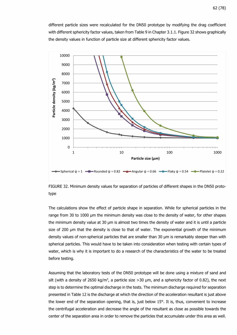
62 (78)
different particle sizes were recalculated for the DN50 prototype by modifying the drag coefficient
with different sphericity factor values, taken from Table 9 in Chapter 3.1.1. Figure 32 shows graphically
the density values in function of particle size at different sphericity factor values.
FIGURE 32. Minimum density values for separation of particles of different shapes in the DN50 proto-
type
The calculations show the effect of particle shape in separation. While for spherical particles in the
range from 30 to 1000 µm the minimum density was close to the density of water, for other shapes
the minimum density value at 30 µm is almost two times the density of water and it is until a particle
size of 200 µm that the density is close to that of water. The exponential growth of the minimum
density values of non-spherical particles that are smaller than 30 µm is remarkably steeper than with
spherical particles. This would have to be taken into consideration when testing with certain types of
water, which is why it is important to do a research of the characteristics of the water to be treated
before testing.
Assuming that the laboratory tests of the DN50 prototype will be done using a mixture of sand and
silt (with a density of 2650 kg/m3, a particle size >30 µm, and a sphericity factor of 0.82), the next
step is to determine the optimal discharge in the tests. The minimum discharge required for separation
presented in Table 12 is the discharge at which the direction of the acceleration resultant is just above
the lower end of the separation opening, that is, just below 15°. It is, thus, convenient to increase
the centrifugal acceleration and decrease the angle of the resultant as close as possible towards the
center of the separation area in order to remove the particles that accumulate under this area as well.
0
1000
2000
3000
4000
5000
6000
7000
8000
9000
10000
1 10 100 1000
Particle density (kg/m
3)
Particle size (µm)
Spherical ψ = 1 Rounded ψ = 0.82 Angular ψ = 0.66 Flaky ψ = 0.54 Platelet ψ = 0.22
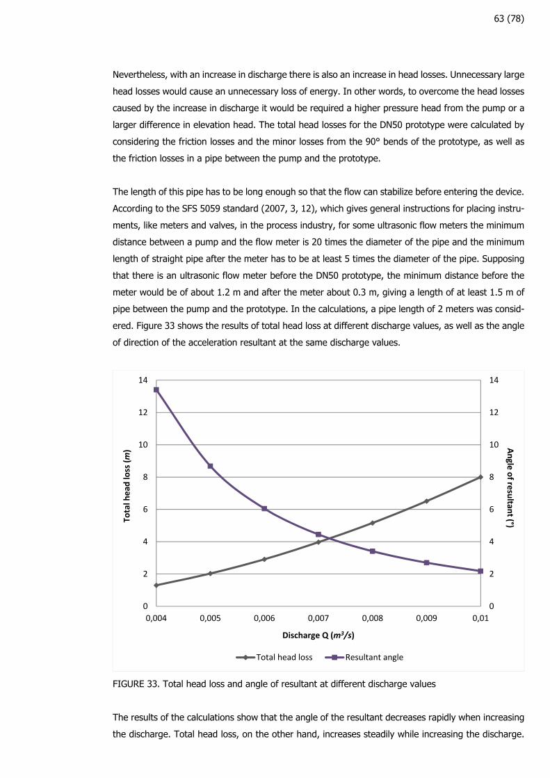
63 (78)
Nevertheless, with an increase in discharge there is also an increase in head losses. Unnecessary large
head losses would cause an unnecessary loss of energy. In other words, to overcome the head losses
caused by the increase in discharge it would be required a higher pressure head from the pump or a
larger difference in elevation head. The total head losses for the DN50 prototype were calculated by
considering the friction losses and the minor losses from the 90° bends of the prototype, as well as
the friction losses in a pipe between the pump and the prototype.
The length of this pipe has to be long enough so that the flow can stabilize before entering the device.
According to the SFS 5059 standard (2007, 3, 12), which gives general instructions for placing instru-
ments, like meters and valves, in the process industry, for some ultrasonic flow meters the minimum
distance between a pump and the flow meter is 20 times the diameter of the pipe and the minimum
length of straight pipe after the meter has to be at least 5 times the diameter of the pipe. Supposing
that there is an ultrasonic flow meter before the DN50 prototype, the minimum distance before the
meter would be of about 1.2 m and after the meter about 0.3 m, giving a length of at least 1.5 m of
pipe between the pump and the prototype. In the calculations, a pipe length of 2 meters was consid-
ered. Figure 33 shows the results of total head loss at different discharge values, as well as the angle
of direction of the acceleration resultant at the same discharge values.
FIGURE 33. Total head loss and angle of resultant at different discharge values
The results of the calculations show that the angle of the resultant decreases rapidly when increasing
the discharge. Total head loss, on the other hand, increases steadily while increasing the discharge.
0
2
4
6
8
10
12
14
0
2
4
6
8
10
12
14
0,004 0,005 0,006 0,007 0,008 0,009 0,01
Angle
of re
sultan
t (°)Total head
loss (m)
Discharge Q (m3/s)
Total head loss Resultant angle
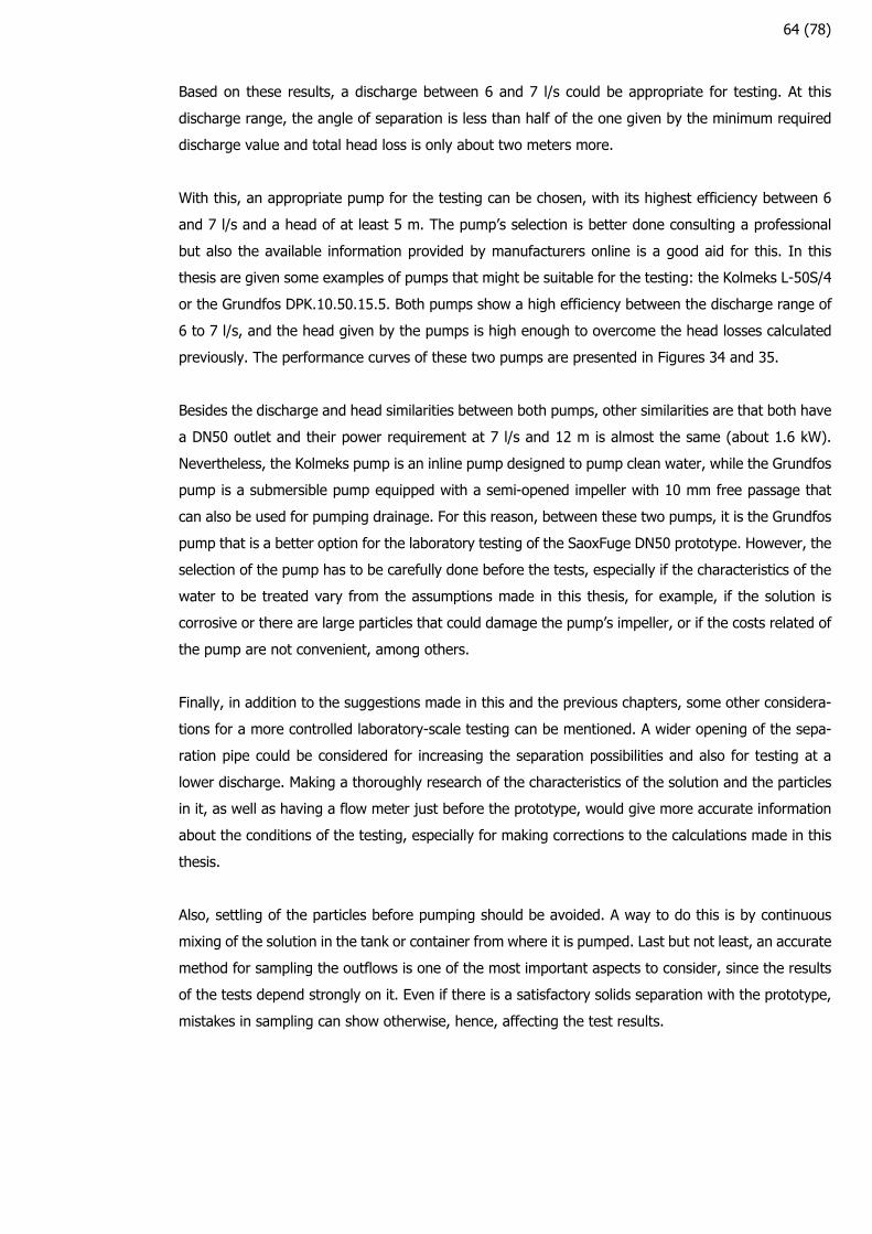
64 (78)
Based on these results, a discharge between 6 and 7 l/s could be appropriate for testing. At this
discharge range, the angle of separation is less than half of the one given by the minimum required
discharge value and total head loss is only about two meters more.
With this, an appropriate pump for the testing can be chosen, with its highest efficiency between 6
and 7 l/s and a head of at least 5 m. The pump’s selection is better done consulting a professional
but also the available information provided by manufacturers online is a good aid for this. In this
thesis are given some examples of pumps that might be suitable for the testing: the Kolmeks L-50S/4
or the Grundfos DPK.10.50.15.5. Both pumps show a high efficiency between the discharge range of
6 to 7 l/s, and the head given by the pumps is high enough to overcome the head losses calculated
previously. The performance curves of these two pumps are presented in Figures 34 and 35.
Besides the discharge and head similarities between both pumps, other similarities are that both have
a DN50 outlet and their power requirement at 7 l/s and 12 m is almost the same (about 1.6 kW).
Nevertheless, the Kolmeks pump is an inline pump designed to pump clean water, while the Grundfos
pump is a submersible pump equipped with a semi-opened impeller with 10 mm free passage that
can also be used for pumping drainage. For this reason, between these two pumps, it is the Grundfos
pump that is a better option for the laboratory testing of the SaoxFuge DN50 prototype. However, the
selection of the pump has to be carefully done before the tests, especially if the characteristics of the
water to be treated vary from the assumptions made in this thesis, for example, if the solution is
corrosive or there are large particles that could damage the pump’s impeller, or if the costs related of
the pump are not convenient, among others.
Finally, in addition to the suggestions made in this and the previous chapters, some other considera-
tions for a more controlled laboratory-scale testing can be mentioned. A wider opening of the sepa-
ration pipe could be considered for increasing the separation possibilities and also for testing at a
lower discharge. Making a thoroughly research of the characteristics of the solution and the particles
in it, as well as having a flow meter just before the prototype, would give more accurate information
about the conditions of the testing, especially for making corrections to the calculations made in this
thesis.
Also, settling of the particles before pumping should be avoided. A way to do this is by continuous
mixing of the solution in the tank or container from where it is pumped. Last but not least, an accurate
method for sampling the outflows is one of the most important aspects to consider, since the results
of the tests depend strongly on it. Even if there is a satisfactory solids separation with the prototype,
mistakes in sampling can show otherwise, hence, affecting the test results.
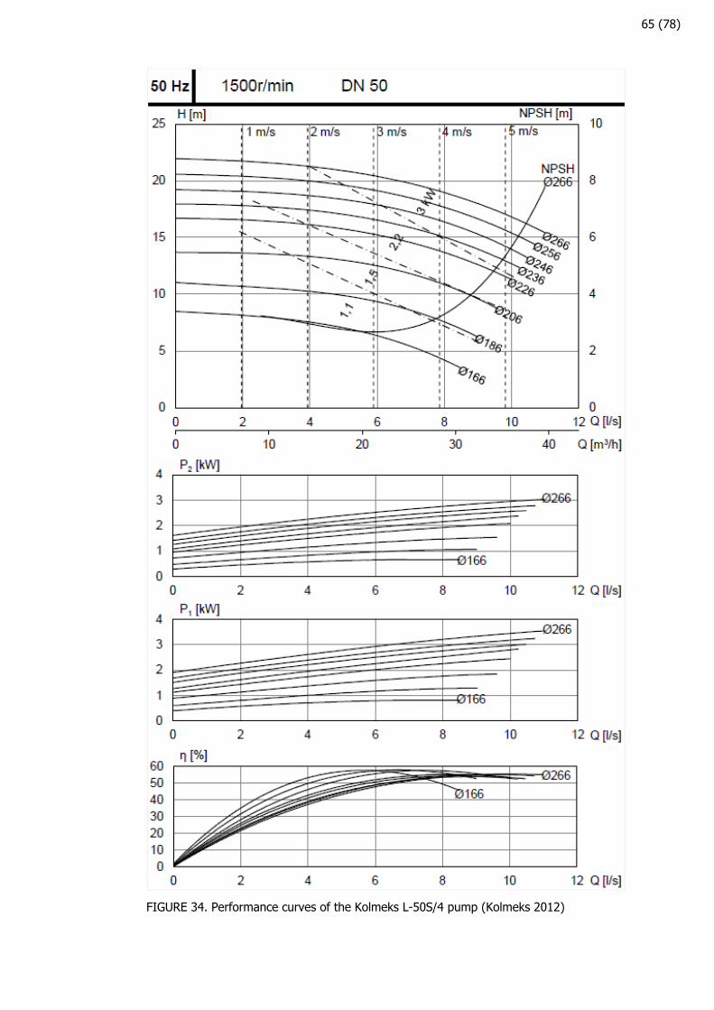
65 (78)
FIGURE 34. Performance curves of the Kolmeks L-50S/4 pump (Kolmeks 2012)
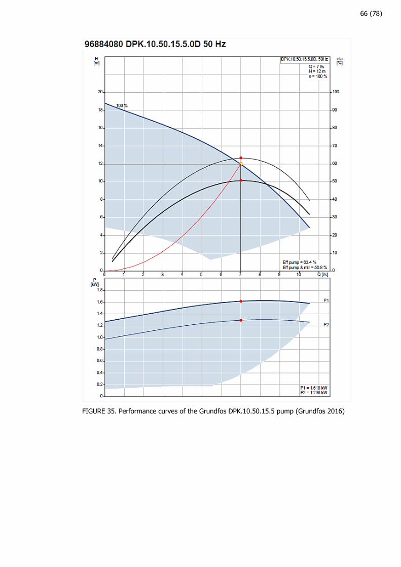
66 (78)
FIGURE 35. Performance curves of the Grundfos DPK.10.50.15.5 pump (Grundfos 2016)
67 (78)
8 CONCLUSIONS
The aim of this thesis was to make a deeper theoretical research of the physical aspects related to
solids separation in the SaoxFuge in order to make a review of the previous tests of the pilot-scale
prototype and find out the possible causes for the inconclusive results of the tests, as well as to
develop a plan for designing and testing a SaoxFuge laboratory-sized prototype for more controlled
conditions of testing.
The first part of the thesis was dedicated to the theoretical research. Firstly, in this research, an
investigation of the physics and hydraulics linked to particle separation and to pipe flow was carried
out. A remarkable realization in this investigation was the theory related to the vortices (known as
Dean vortices) generated in curved pipes due to the influence of the centrifugal force. Nevertheless,
due to the complexity of the study of these vortices, in the calculations made in the thesis, it was
assumed that these vortices do not happen in the SaoxFuge.
The particle separation theory contained basic explanations of the principal characteristics of particles,
like size, shape, and density, as well as the basic theory related to particle settling. The latter high-
lighted the effect of the drag that a particle experiences when moving within a fluid. Also, the way
that particles in a certain solution settle has to be determined, in many cases, with sedimentation
tests in the laboratory.
In the last part of the theoretical research, the solids separation methods most commonly used in
water treatment facilities were described. The purpose of the information gathered in this section was
to give some references for comparing the SaoxFuge to these methods. From this, it was noticed that,
for example, achieving with the SaoxFuge a centrifugal acceleration that is close to the one achieved
by a centrifuge is quite challenging. However, one of the main advantages that the SaoxFuge offers
is a retention time much shorter and a needed space much smaller compared to other methods.
In the second part of the thesis, the main conditions of the previous testing of the SaoxFuge proto-
types in the summer of 2015 were described and also the plan for the laboratory-sized prototype
sizing and testing was developed. The solids separation in the prototype was considered possible if
two conditions were met: that a particle traveling in the center of the pipe could travel during the
retention time a distance equal or greater than the size of the inner radius of the pipe, and that the
direction of the resultant of the acceleration of the particle was towards the opening area of the
separation pipe of the prototype.
With the information of the conditions at which the testing of the prototypes was made, it was possible
to find possible causes for the inconclusive results of the tests. The calculations made showed that
the discharge at which the tests were carried out was not enough to accelerate the particles in a
direction towards the area of the opening of the separation pipe, even though the particles could
travel a distance much larger than the radius of the pipe during the retention time.
68 (78)
An important observation was that by the distance that the particle could travel during the retention
time was not affected by changes in discharge. The reason for this was that even if an increase in
discharge would cause the settling velocity of the particle to increase, it would also cause the retention
time to decrease in the same proportion. So, changing the prototype dimensions, especially adding
turns of the spiral, would be a better way to increase the retention time in order to give a certain
particle more time to travel the length of the radius of the pipe.
Lastly, the development of the plan for the laboratory-scale testing was made with the aid of an Excel
workbook. All the parameters and formulas used in the calculations related to the solids separation in
the SaoxFuge prototype were gathered in this workbook. Warnings are showed in case the angle of
the resultant of the acceleration is too big, or if the retention time is too short for the particle to travel
the length of the radius of the pipe. In addition to this, information of the pump and fittings before
the prototype can be added, and also a warning sign appears if there is risk of pump cavitation. The
workbook contains also information about some parameters, like water properties at different tem-
peratures and roughness factors of different pipe materials, as well as diagrams of the sizing param-
eters of the prototype and a Moody diagram.
The plan for the laboratory-scale prototype considered the characteristics of the solids commonly
found in municipal wastewater and the comparison between three different prototype sizes. The re-
sults showed that a prototype of size DN50 would be convenient for the testing at a laboratory scale.
The optimal particle characteristics for separation with this prototype would be rounded or spherical
particles with a size greater than 30 µm and a density between 1100 and 2000 kg/m3. The calculations
also showed that the more the particle shape differs from that of a sphere, the more difficult its
separation will be. Flow conditions optimal for this testing would be between 6 and 7 l/s.
The results of this thesis are a general guide for developing a testing plan of the SaoxFuge prototype.
The characteristics of the solution to be treated and of the particles in it are the main parameters for
the prototype sizing, so it is of main relevance to know this information beforehand. Also a wider
opening of the separation pipe or adding turns to the spiral could be considered for increasing the
solids separation possibilities of the prototype. When testing the prototype, an adequate sampling
method is essential for having trustworthy test results.
In the future, a deeper analysis of the phenomena occurring in the SaoxFuge must be considered.
Numerical analysis and computational fluid dynamics would give a better understanding of the flow
conditions inside the SaoxFuge and the vortices caused by the spiral shape of the pipe and the turbu-
lent flow. Tomography can also be added to complement the testing of the prototypes. It would help
to study how the particles move inside the prototype and to identify critical zones.
69 (78)
REFERENCES
Benjamin, Mark M. & Lawler, Desmond F. 2013. Water quality engineering: physical/chemical treat-
ment processes. Hoboken, New Jersey: John Wiley & Sons, Inc.
Benson, Harris. 1995. University Physics. Revised edition. New York: John Wiley & Sons, Inc.
Croft, Anthony; Davison, Robert & Hargreaves, Martin. 2001. Engineering Mathematics: a foundation
for electronic, electrical, communications, and systems engineers. Third edition. Harlow, Essex: Pear-
son Education Ltd.
Droste, Ronald L. 1997. Theory and practice of water and wastewater treatment. New York: John
Wiley & Sons, Inc.
Estrada Reynoso, Priscila. 2015. Kiintoaineenerotuslaitteen SaoxFugen tutkimus. KaivosVV -hanke,
Yara Suomi Oy:n Siilinjärven rikastamo. [Electronic report] Located in the author’s electronic files.
Forsythe, William Elmer. 1954; 2003. Smithsonian physical tables. Ninth edition. Norwich, New York:
Knovel. [Accessed on 16 February 2016] Available from:
https://app.knovel.com/web/view/swf/show.v/rcid:kpSPTRE008/cid:kt002VRH31/view-
erType:pdf/root_slug:smithsonian-physical?cid=kt002VRH31&page=16&q=effect%20of%20pres-
sure%20upon%20viscosity&b-q=effect%20of%20pressure%20upon%20viscosity&sort_on=de-
fault&b-subs
Geologinen tutkimuslaitos. 1982. Perustietoa malminetsijälle. Opas 9. [Web document] Espoo: Geo-
loginen tutkimuslaitos. [Accessed on 31 March 2016] Available from:
http://tupa.gtk.fi/julkaisu/opas/op_009.pdf
Graebel, W. P. 2001. Engineering fluid mechanics. New York: Taylor & Francis Publishers.
Grundfos Pumps Corporation. 2016. Grundfos Product center. Find product. [Accessed on 15 April
2016] Available from:
http://product-selection.grundfos.com/product-detail.product-detail.html?custid=GMA&productnum-
ber=96884080&qcid=86311525
Hamill, Les. 2011. Understanding Hydraulics. Third edition. Basingstoke, Hampshire: Palgrave Mac-
millan.
Holdich, Richard G. 2002. Fundamentals of particle technology. Shepshed, Leicestershire: Midland
Information Technology and Publishing. [Accessed on 19 February 2016] Available from:
http://particles.org.uk/particle_technology_book/particle_book.htm
70 (78)
Karassik, Igor J; Messina, Joseph P.; Cooper, Paul & Heald, Charles C. 2001. Pump Handbook. Third
edition. New York: McGraw-Hill.
Keränen, Mikko. 2015. Mill manager at Yara Finland Siilinjärvi site. [Email] Receivers Priscila Estrada
Reynoso, Eero Antikainen and Pasi Pajula. Sent on 5 June 2015.
Knight, Randall D. 2014. Physics for Scientists and Engineers: a strategic approach with modern phys-
ics. Third edition. Harlow, Essex: Pearson Education Ltd.
Kolmeks Oy. 2012. Materiaalipankki. Datalehdet. Keskipakopumput. L_-50S/4. [Accessed on 15 April
2016]. Available from: http://www.kolmeks.fi/materiaalipankki/datalehdet/keskipakopumput
Kundu, Pijush K.; Cohen, Ira M. & Dowling, David R. 2012. Fluid Mechanics. Fifth edition. Oxford:
Elsevier Inc.
Kuriyama of America, Inc. 2013. Layflat discharge hoses. [Web catalogue]. Schaumburg, Illinois: Ku-
riyama of America, Inc. [Accessed on 31 March 2016] Available from:
http://products.kuriyama.com/asset/Kuriyama-Layflat-Products-16-Pg--Catalog_LR_-Final-3-01-
13GK.pdf
Mezger, Thomas G. 2006. The rheology handbook: for users of rotational and oscillatory rheometers.
Second revised edition. Hannover: Vincentz Network GmbH & Co. [Accessed on 3 February 2016].
Available from:
https://books.google.fi/books?id=N9Fdn0MEI-
DIC&pg=PA29&hl=fi&source=gbs_toc_r&cad=3#v=onepage&q&f=false
Peker, Sümer M. & Helvaci, Şerife Ş. 2008. Solid-liquid two phase flow. Amsterdam, NL: Elsevier.
[Accessed on 19 February 2016] Available from:
https://app.knovel.com/web/view/pdf/show.v/rcid:kpSLTPF001/cid:kt00C50672/view-
erType:pdf/root_slug:solid-liquid-two-phase/url_slug:classification-separation?cid=kt00C50672&b-
q=hydrocyclone&b-subscription=TRUE&b-group-by=true&b-search-type=tech-reference&b
RIL. 2003. 124-1 Vesihuolto I. Helsinki: Suomen Rakennusinsinöörien Liitto RIL r.y.
RIL. 2003. 124-1 Vesihuolto II. Helsinki: Suomen Rakennusinsinöörien Liitto RIL r.y.
SansOx. 2015. SansOx Solutions 2015. [Power Point presentation] Helsinki. Received via email from
Juhani Pylkkänen on 3 November 2015.
SansOx. 2016. [Website] [Accessed on 13 April 2016] Available from: www.sansox.fi
71 (78)
SFS 5059. 2007. Instrumentation. Placing of Process Instruments. Second Edition. Helsinki: Finnish
Standards Association.
Tchobanoglous, George; Stensel, H. David; Tsuchihashi, Ryujiro; Burton, Franklin; Abu-Orf, Moham-
mad; Bowden, Gregory & Pfrang, William. 2014. Wastewater engineering: treatment and resource
recovery. Fifth edition. New York: McGraw-Hill Education.
Tuomenlehto, Ari; Holmlund, Eero; Huuskonen, Maija; Makkonen, Heikki & Surakka, Jarkko. 2014.
Insinöörin matematiikka. First edition. Helsinki: Edita.
United Nations Committee on Economic, Social, and Cultural Rights. 2002. General Comment No. 15.
The right to water (arts. 11 and 12 of the International Covenant on Economic, Social and Cultural
Rights). Geneva. [Accessed on 13 April 2016]. Available from:
https://documents-dds-ny.un.org/doc/UNDOC/GEN/G03/402/29/PDF/G0340229.pdf?OpenElement
World Health Organization (WHO). 2015. Media centre. Fact sheets. Drinking water. [Website] June
2015. [Accessed on 28 January 2016] Available from:
http://www.who.int/mediacentre/factsheets/fs391/en/

APPENDIX 1. SAOXFUGE SPIRAL PROTOTYPE
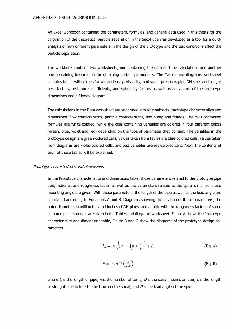
APPENDIX 2. EXCEL WORKBOOK TOOL
An Excel workbook containing the parameters, formulas, and general data used in this thesis for the
calculation of the theoretical particle separation in the SaoxFuge was developed as a tool for a quick
analysis of how different parameters in the design of the prototype and the test conditions affect the
particle separation.
The workbook contains two worksheets, one containing the data and the calculations and another
one containing information for obtaining certain parameters. The Tables and diagrams worksheet
contains tables with values for water density, viscosity, and vapor pressure, pipe DN sizes and rough-
ness factors, resistance coefficients, and sphericity factors as well as a diagram of the prototype
dimensions and a Moody diagram.
The calculations in the Data worksheet are separated into four subjects: prototype characteristics and
dimensions, flow characteristics, particle characteristics, and pump and fittings. The cells containing
formulas are white-colored, while the cells containing variables are colored in four different colors
(green, blue, violet and red) depending on the type of parameter they contain. The variables in the
prototype design are green-colored cells, values taken from tables are blue-colored cells, values taken
from diagrams are violet-colored cells, and test variables are red-colored cells. Next, the contents of
each of these tables will be explained.
Prototype characteristics and dimensions
In the Prototype characteristics and dimensions table, those parameters related to the prototype pipe
size, material, and roughness factor as well as the parameters related to the spiral dimensions and
mounting angle are given. With these parameters, the length of the pipe as well as the lead angle are
calculated according to Equations A and B. Diagrams showing the location of these parameters, the
outer diameters in millimeters and inches of DN pipes, and a table with the roughness factors of some
common pipe materials are given in the Tables and diagrams worksheet. Figure A shows the Prototype
characteristics and dimensions table, Figure B and C show the diagrams of the prototype design pa-
rameters.
∗ Eq.A
∗
Eq.B
where lp is the length of pipe, n is the number of turns, D is the spiral mean diameter, L is the length
of straight pipe before the first turn in the spiral, and θ is the lead angle of the spiral.
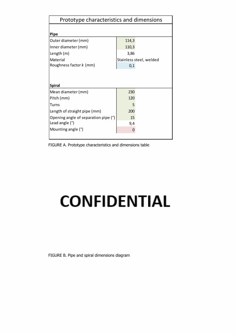
FIGURE A. Prototype characteristics and dimensions table
FIGURE B. Pipe and spiral dimensions diagram
Pipe
Outer diameter (mm) 114,3
Inner diameter (mm) 110,3
Length (m) 3,86
MaterialRoughness factor k (mm) 0,1
Spiral
Mean diameter (mm) 230
Pitch (mm) 120
Turns 5
Length of straight pipe (mm) 200
Opening angle of separation pipe (°) 15Lead angle (°) 9,4
Mounting angle (°) 0
Prototype characteristics and dimensions
Stainless steel, welded
FIGURE C. Lead angle of spiral and angle of the opening of the separation pipe
Flow characteristics
In the Flow characteristics table are the values related to the hydraulics of the flow and the centrifugal
acceleration and resultant values. There are three main sections: properties of the fluid, hydraulics
and physics (Figure D). The values for properties of the fluid, usually water, depend on its temperature
and, based on it, the values for density, viscosity, and vapor pressure of the water can be taken from
a table in the Tables and diagrams worksheet. The atmospheric pressure and vapor pressure of water
are relevant to determine if there is a risk of pump cavitation in the Pump and fittings table. The
pressure head is calculated by subtracting the total head losses to the head given by the pump.
In the hydraulics section, the values for discharge and friction factor are introduced for calculations
of the flow velocity, Reynold’s number, friction losses, minor losses, total head losses and retention
time. All of these are calculated as presented in Chapter 5 in this thesis. Minor losses are calculated
in the Pump and fittings table. The volume taken in the calculation of the retention time is calculated
by multiplying the cross-sectional area of the pipe times its length. The friction factor can be deter-
mined from the Moody diagram in the Tables and diagrams worksheet.
In the physics section, the gravitational and centrifugal acceleration as well as the magnitude and
angle of direction of the acceleration resultant are presented. The flow velocity and the spiral’s mean
diameter are taken for the centrifugal acceleration calculation as shown in Chapter 5. The calculation
of the magnitude and angle of direction of the resultant is done according to Equations C and D.
2 180 90 Eq.C
Eq.D
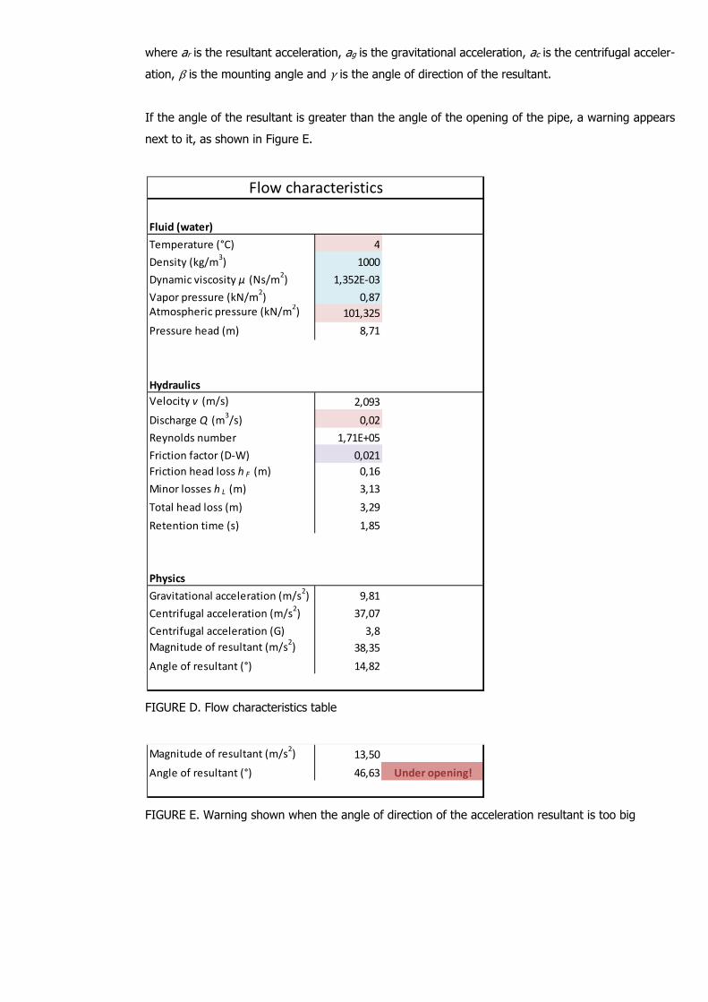
where ar is the resultant acceleration, ag is the gravitational acceleration, ac is the centrifugal acceler-
ation, β is the mounting angle and γ is the angle of direction of the resultant.
If the angle of the resultant is greater than the angle of the opening of the pipe, a warning appears
next to it, as shown in Figure E.
FIGURE D. Flow characteristics table
FIGURE E. Warning shown when the angle of direction of the acceleration resultant is too big
Fluid (water)
Temperature (°C) 4
Density (kg/m3) 1000
Dynamic viscosity µ (Ns/m2) 1,352E‐03
Vapor pressure (kN/m2) 0,87
Atmospheric pressure (kN/m2) 101,325
Pressure head (m) 8,71
Hydraulics
Velocity v (m/s) 2,093
Discharge Q (m3/s) 0,02
Reynolds number 1,71E+05
Friction factor (D‐W) 0,021
Friction head loss h F (m) 0,16
Minor losses h L (m) 3,13
Total head loss (m) 3,29
Retention time (s) 1,85
Physics
Gravitational acceleration (m/s2) 9,81
Centrifugal acceleration (m/s2) 37,07
Centrifugal acceleration (G) 3,8
Magnitude of resultant (m/s2) 38,35
Angle of resultant (°) 14,82
Flow characteristics
Magnitude of resultant (m/s2) 13,50
Angle of resultant (°) 46,63 Under opening!
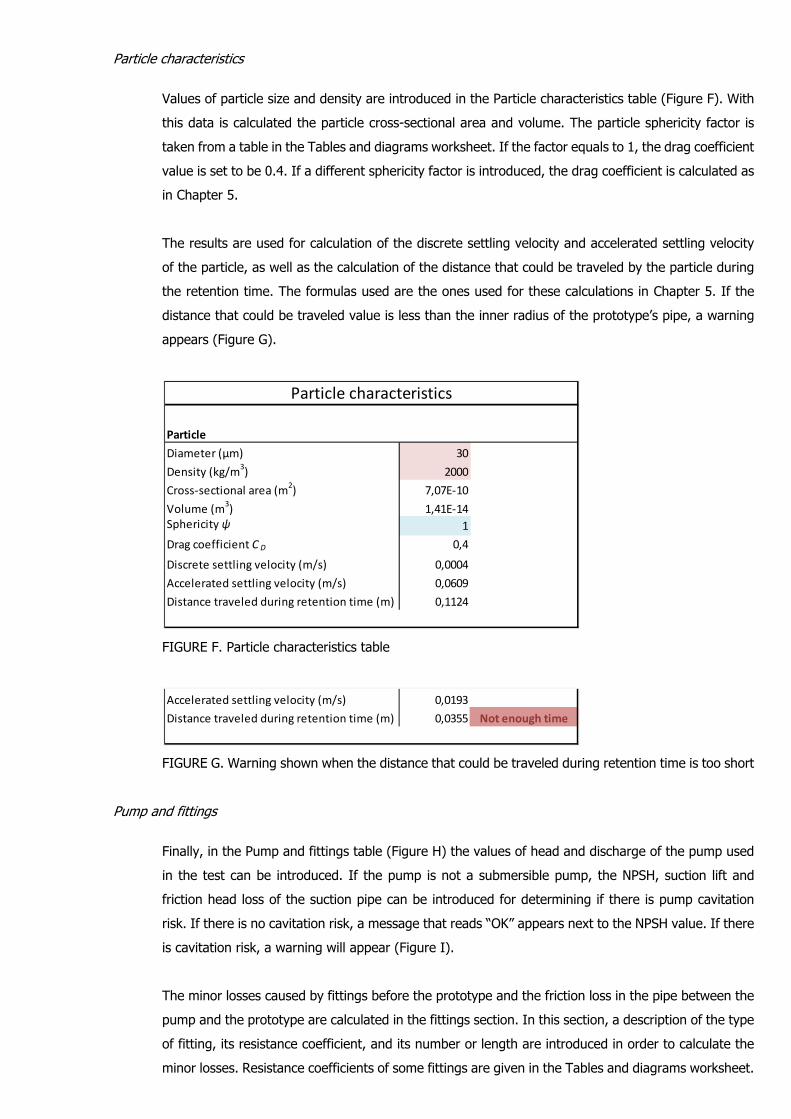
Particle characteristics
Values of particle size and density are introduced in the Particle characteristics table (Figure F). With
this data is calculated the particle cross-sectional area and volume. The particle sphericity factor is
taken from a table in the Tables and diagrams worksheet. If the factor equals to 1, the drag coefficient
value is set to be 0.4. If a different sphericity factor is introduced, the drag coefficient is calculated as
in Chapter 5.
The results are used for calculation of the discrete settling velocity and accelerated settling velocity
of the particle, as well as the calculation of the distance that could be traveled by the particle during
the retention time. The formulas used are the ones used for these calculations in Chapter 5. If the
distance that could be traveled value is less than the inner radius of the prototype’s pipe, a warning
appears (Figure G).
FIGURE F. Particle characteristics table
FIGURE G. Warning shown when the distance that could be traveled during retention time is too short
Pump and fittings
Finally, in the Pump and fittings table (Figure H) the values of head and discharge of the pump used
in the test can be introduced. If the pump is not a submersible pump, the NPSH, suction lift and
friction head loss of the suction pipe can be introduced for determining if there is pump cavitation
risk. If there is no cavitation risk, a message that reads “OK” appears next to the NPSH value. If there
is cavitation risk, a warning will appear (Figure I).
The minor losses caused by fittings before the prototype and the friction loss in the pipe between the
pump and the prototype are calculated in the fittings section. In this section, a description of the type
of fitting, its resistance coefficient, and its number or length are introduced in order to calculate the
minor losses. Resistance coefficients of some fittings are given in the Tables and diagrams worksheet.
Particle
Diameter (µm) 30
Density (kg/m3) 2000
Cross‐sectional area (m2) 7,07E‐10
Volume (m3) 1,41E‐14
Sphericity ψ 1
Drag coefficient C D 0,4
Discrete settling velocity (m/s) 0,0004
Accelerated settling velocity (m/s) 0,0609
Distance traveled during retention time (m) 0,1124
Particle characteristics
Accelerated settling velocity (m/s) 0,0193
Distance traveled during retention time (m) 0,0355 Not enough time
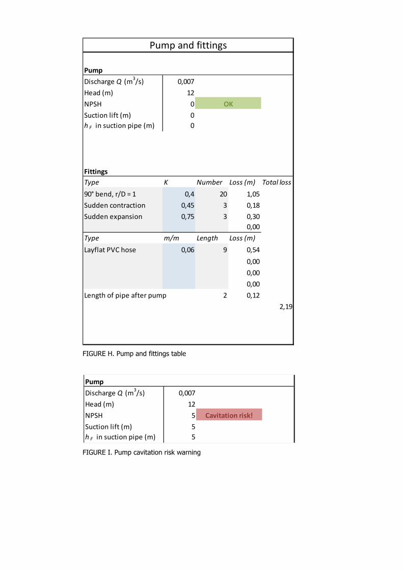
FIGURE H. Pump and fittings table
FIGURE I. Pump cavitation risk warning
Pump
Discharge Q (m3/s) 0,007
Head (m) 12
NPSH 0
Suction lift (m) 0
h F in suction pipe (m) 0
Fittings
Type K Number Loss (m) Total loss
90° bend, r/D = 1 0,4 20 1,05
Sudden contraction 0,45 3 0,18
Sudden expansion 0,75 3 0,30
0,00
Type m/m Length Loss (m)
Layflat PVC hose 0,06 9 0,54
0,00
0,00
0,00
Length of pipe after pump 2 0,12
2,19
Pump and fittings
OK
Pump
Discharge Q (m3/s) 0,007
Head (m) 12
NPSH 5
Suction lift (m) 5
h F in suction pipe (m) 5
Cavitation risk!