van der waals theory for solids

PHYSICAL REVIEW E VOLUME 50, NUMBER 4 OCTOBER 1994

van der Waals theory for solids

A.Daanoun, C. F. Tejero and M. BausFaculte des Sciences, Code Postal 881, Universite Libre de Bruzelles, B-1050 Brussels, Belgium

Facnltad de Ciencias Fisicas, Universidad Complatense de Madrid, F 280-$0 Madrid, Spain(Received 9 May 1994)

In analogy with the well-known theory for Huids, a van der Waals theory for solids is proposed.It is shown that, in agreement with recent predictions, the competition between the van der Waalsloop of the Quid and the van der Waals loop of the solid can produce three different types of phasediagrams for a simple Quid. This could be of relevance to the phase behavior of colloidal dispersions.

PACS number(s): 64.70.Dv, 64.10.+h, 82.70.—y

I. INTRODUCTION

The van der Waals (vdW) theory [1] is remarkable inthat, although based on very simple ideas about the in-termolecular interactions, it is nevertheless capable of de-scribing the complex behavior associated with the liquid-gas transition, including its critical point, with very sim-ple algebraic means. As such its value cannot be overes-timated, not only as a pedagogical tool but also becauseit did pave the way to the improved vdW-like theorieswhich lie at the heart of our present understanding ofthe liquid state [2].

Recently it was found, both by simulations [3] and bytheory [4], that a vdW loop can develop not only in thefluid phase, as in the original vdW theory, but also inthe solid phase. This then suggests that there shouldbe a solid-phase counterpart to the original fluid-phasevdW theory. In the present study, we will introduce sucha theory for the vdW loop of the solid and explore itsconsequences for the phase diagram. The purpose of thisstudy is hence to yield a better understanding of the moreexact results of [3,4] and to provide a simple analysis ofthe phase behavior of colloidal dispersions for which someof these phenomena could be observable.

In the following, we recall the approximations behindthe vdW theory (Sec. II) and derive the vdW theory forthe fluid (Sec. III) and the solid (Sec. IV) phases. Theresulting phase behavior is discussed in Sec. V, while ourconclusions are gathered in Sec. VI.

II. THE vdW APPROXIMATION

where P = 1/kjsT with T the temperature and ks Boltz-mann's constant, and H—:H(I'), the Hamiltonian of oursystem, is defined over the phase space I' with j dI' edenoting the usual canonical partition function. Let Fodenote the free energy of a reference system with Hamil-tonian Ho = Ho(I') defined over the same phase spaceI' and related to Fa by a relation similar to (2.1). Sub-tracting both relations we obtain, after some rewriting,

(2.2)

where ()o denotes the canonical average over the refer-ence system. Using the convexity of the logarithm wehave

P(H Hii)—) ~—

(l P(H Ho))— —(2.3)

where the right hand side of (2.3) equals P((H —Ho)—)s,and combining with (2.2) we obtain

F —Fp & ((H —Hp))p (2.4)

which is the announced Gibbs-Bogoliubov inequality.Equation (2.4) can be rewritten as

F & Fi ——Fo+ ((H —Hp))(), {2.5)

1F & Fi = Fp + — dri dr2 p2(ri, r2) [V(ri2)2

where F~ is identical to the first-order expansion of Faround Fo. When K and Ho dier only by the nature ofthe pair-potential we have for (2.5)

—pr = in f rti' e ~~i", (2.1)

There are many ways to present the vdW theory. In or-der to obtain a unified presentation for both the fluid andthe solid phases we will start &om the Gibbs-Bogoliubovinequality [2] but this is by no means the only way toproceed. The Gibbs-Bogoliubov inequality itself can alsobe derived in various ways. A short derivation goes asfollows. The definition of the Helmholtz free energy Freads

—V, (r»)], (2.6)

where ri2 ——~ri —r2~, while V(ri2) and Vo(ri2) denote,respectively, the pair potential of the system and of thereference system, and p2(ri, r2) is the pair density of thereference system. The vdW theory is based on taking, asa reference system, a system with purely repulsive forces.To this end we will split the total pair potential, V =V~ + V~, into a repulsive (VR) and an attractive (V~)part and take Vo = V~ so that (2.6) becomes with thischoice of reference system:

1063-651X/94/50(4)/2913(12)/$06. 00 50 2913 1994 The American Physical Society

2914 A. DAANOUN, C. F. TEJERO, AND M. BAUS

1F1 —FR +

2~&1 ~j 2 P2 ~1 &2 VA ~12

(2 7)

where I"~ and p2 (ri, r2) denote, respectively, the freeenergy and the pair density of a reference systemwith purely repulsive forces corresponding to the pair-potential V~(ri2). From the exact inequality (2.7) oneobtains the vdW theory by introducing three approxi-mations. First, one takes the upper bound F1 as theestimate of the &ee energy F:

where pi (r) is the one-body density of the reference sys-tem with V~(r) as pair potential. Notice that because of(2.9) the vdW theory is a mean-field approximation. Thevd%' approximation, F„g~, to the exact Bee energy, F,of a system with the pair potential, V = VR + VA, reads,thus,

R RF gw —+R + dri dr2 pi (ri) pi (r2) VA(+12)2

(2.10)

d&1 d&2 P2 &1 &2 VA ~12 (2.8)

~&2P2» &2

dr1 dr2P1 r1 P1 r2 VA r12, 2.9

and, second, one approximates the exact upper boundF1 by neglecting all the correlations within the domainof V~(ri2), i.e. ,

but for notational facility we will henceforth drop thesubscript vdW on F„gear. The final ingredient of thevdW theory, which can be considered as the third ap-proximation, consists in approximating VR by a simplehard-sphere (HS) potential which leads then to an ex-plicit expression for FR = FHS when the latter is obtainedby thermodynamic integration of a simple HS equation ofstate. We will thus write the pair potential V(r) hence-forth as, V(r) = e[PHs(z) + P~(z)], where z = r/o' witho. the HS diameter:

SW

(x) (b)

HS

I P (n=6)

FIG. 1. In the van der Waals(vdW) theory the repulsivepart (PR) of the total pair po-tential (PR + P~) is, as shownin (a), represented by a sim-

ple hard-sphere (HS) interac-tion. For the attractive part(P~) we will, for the purpose ofillustration, consider two cases:(b) a square-well (SW) attrac-tion of range p, and (c) an in-verse-power (IP) attraction ofindex n [see also (2.11—2.14);the IP potential shown herecorresponds to n = 6].

(x}

-1

50 van der WAALS THEORY FOR SOLIDS 2915

oo, x&14~s(*) =

0 (2.11)

and e the well depth of the attractions described by

(3.5) along an isotherm. As usual in the vdW theory,fus will be prescribed by adopting an equation of statefor the HS. For the latter we take a simple &ee-volumeapproximation:

0, &&1AA(x) = '4( (2.12) Ppas(p)

p) g(1

1 —g(3.6)

( )1, 1&x&1+p0, x &1+p (2.13)

as the prototype of a discontinuous potential, and (b) aninverse power (IP) potential of index n

where P(x) & 0, and P(x) tending to zero as x tendsto inhnity. Below we will moreover illustrate our resultswith the help of two simple forms of attraction: (a) asquare well (SW) of range p

so that (1 —ri)V is the average volume freely accessibleto the HS in a fluid of volume V. We write g = p/po, sothat po is the maximum density (p & po) for which theHS Quid can exist. The precise value of po is immaterialhere but will be discussed further in Sec. V. Notice thatthe standard vdW theory follows only when taking po ——

6/pro's, in which case rI is the packing fraction. Using(3.6), Eq. (3.4) can be easily integrated yielding for (3.2)and (3.5):

14(x) = —;n&3 (2.14) f =t Cz+ln

1 —rl(3.7)

as the prototype of a continuous potential (see Fig. 1).Obviously, many other choices are possible.

p, =t Cy+ln +7l

1 —g 1 —g—2gI', (3 8)

III. THE vdW THEORY OF THE FLUID PHASE

Although this theory is very well known [1], in orderto stress the analogy with the developments of the nextsection, we briefly repeat the main steps here. For auniform fluid phase we have

p (r) = pHS (3.1)

f = f~s+ &f

with, on using (3.1) and (2.12),

(3.2)

b,f = — dr V~(r) = 2vrprr — dxx P(x) (3.3)2E' 1

together with

f„,=t in(pA') —1+ P~

""',P —1~, (3.4)o P ( P )

where t = k~T/e is the reduced temperature and A thethermal de Broglie wavelength of the HS. From f one canobtain the reduced chemical potential, p = p/e, and thereduced pressure, p = po' /e, from

where p is the number density of the N particles. Usingdimensionless free energies per particle, f = F/Ne andf~s ——F~s/Ne, we rewrite (2.10, 2.11) as

p'7

poo 1 —g(3.9)

where

Cf = ln(poA ) —1; I' = 2z pocr dx x P(x), (3.10)1

or

I'sw = —7rpoo' [(1+p) —1] = 2z porr p ~

1+p + —p2 s s s (3 )

(3.11a)

27rpoo' s 1 ( 1I'yp = = 2~poo

n —3 1(3.11b)

Qp t9 p7 g 2 (3.12)

for, respectively, a SW attraction (a) of range p, and anIP attraction (b) of index n (n ) 3). It is also seen from(3.11) that for attractions of short range (p « 1 orn &) 1) 1/n plays the same role as p. The consequencesof the vdW theory embodied in (3.7—3.9) are well known.The form of (3.7) leads to a vdW loop. To obtain thecorresponding critical point (rk, t„p,) one solves

~(pf).p= ) p=gp Bv

(3.5)

which yields on using (3.9)

= —I'.1 8 p 1

27 Cpa 27(3.13)

where v = 1/pa s. We recall also that (3.4) is nothing butthe exact relation between the (HS) free energy and the(HS) equation of state or compressibility factor (Ppzs/p),which results kom integrating the pressure equation of

The complete fluid(Eq)-fluid(Fz) coexistence curve canalso be obtained by solving the two-phase coexistenceconditions:


p(r)i t) =P(r)2, t), (3.14a) r)2(I —r)i) 27 t,ln = —(r)2 —r)a)(2 —r)i —i)2): (3.»b)

r)i(l —r)2) 8

p, (r)i, t) = P(r)2, t), (3.14b)

8(ni+ n2)(I —ni)(I —n2) =

27 —,— (3.15a)

where gl denotes the value of g for the low-density fluidphase Fl, and g2 that of the high-density fluid phase I"2.From (3.8,3.9) we obtain for (3.14)

which since (3.15) depends only on t/t, and r)/rk embod-ies a law of corresponding states, leading to the universalcoexistence curves in the t —q and p —t planes shownin Fig. 2. Notice also that the law of rectilinear diam-eters which states that the midpoints of the coexistingdensities lie on a straight line in the t —r) diagram [5],r)i + r)2 —2t/3t„although very well satisfied near thecritical point (see Fig. 2) is not an exact property of(3.15).

1.2

(a)IV. THE vdW THEORY OF THE SOLID PHASE

0.8-

For a perfect crystal with lattice sites r~, we have in-stead of (3.1)

0.6— pi (r) = ) ip(r rj!i

0.4-

0.2—

where p(r —r~) describes the normalized (f droop(r) =-- I,'density profile around the site at r~. Substituting (4.1)into (2.10) yields for (3.2)

dr' p(r —r, )

(4.2)

1.2—

o.s I

while fHs is still given in terms of the HS equation of stateby (3.4). For the equation of state of the HS solid we will

adopt again a very simple expression [cf. (3.6)]. Like incell theory [6], we will use a free-distance approximatiori:

~PHs(P)

p 1 —P/3

0.4 &

0.2 1

0 I I I I I

0 02 04 06 08 1 12

FIG. 2. The universal coexistence curves in (a) thetemperature(t)-density(ri) and (b) the pressure (p)-temperature(t) planes for the Huid(Fi)- Huid(F2) coexistenceas obtained from the vdW free energy (3.7). Here Fi denotesthe Iow-density Huid (or gas) and Fz the high-density fluid (orliquid) phase in which the Huid phase F separates for temper-atures below the critical temperature. All quantitities are ref-ered to their critical point (full dot) values of (3.13). It is alsoseen that the midpoints of the coexisting densities (dash-dotline) is approximately a linear function of the temperature inthe vicinity of the critical point (the straight line is given asa guide to the eye). This corresponds to the so-called law ofrectilinear diameters [5] being approximately satisfied.

3P,p 3

p p—p 1

(4.4)

and we recover the usual free-volume behavior whichholds well [2] for HS at high densities [7] (cf. Fig. 3).In the opposite limit b ~ 0, (4.3) exhibits a free-particlebehavior [whereas (4.4) does not] so that, (3.4) can againbe easily integrated w'hen (4.3) is used, yielding

so that I' "3(1—6 ~s) is the average distance over whichthe HS can freely move in the HS crystal of volume V.We again write 8 = p/p, p, so that p, p is the maximunivalue of the density p for which the crystal can exist,i.e., p, p is the density at close packing (cp) of the givenlattice structure. Except for the change from free volumeto free distance, (4.3) is similar in spirit to (3.6), with p,.„being the equivalent for the solid of po for the fluid. Forp -+ p„p, (4.3) implies


65

55

45

(4.7) while for a Buid we have p(r) = p and (4.8) restores(3.3).

To proceed we can rewrite the lattice sum (4.7) interms of a sum over spherical shells of sites centeredaround the site at the origin, with the jth shell containingn~ sites:

35

25

sites shells

&f = --):4(z. ) = -- ) . n~ &(z~)2 2

(4.9)

15

50.55 0.6 0.65

KG PE

0.7 0.75

FIG. 3. The HS-compressibility factor (Pp/p) vs theHS-packing fraction (s'po /6) as obtained from the simpleEq. (4.3) (broken line) compared to the fit to the computersimulations of a fcc-HS solid (full line) as proposed by Hall[71.

1b,f = ——n1 p(z1),

2(4.10)

which is similar to the approximation already used else-where [8) for a purely repulsive potential. Notice thatthe site (shell) at the origin, zo ——0 and no ——1, does notcontribute to (4.9) because P(0) is a constant which canalways be put equal to zero, since in the presence of aHS repulsion p(z) need to be defined only for z ) 1 [cf.(2.12)]. Ordering the remaining shells by increasing radii(z1 ( z2 ( zs ) we can for a decreasing p(z) only keepthe dominant term:

fHs = t[C, + lnh —3 ln(1 —b / )]—:t[C, —3 ln(z1 —1)], (4 5)

where n1 is the number of nearest neighbors and x1 thereduced nearest-neighbor distance of the given crystalstructure as it appears already in (4.5,4.6). The presentvdW theory, (4.5) and (4.10), yields, thus,

where

C, = in(p, pAs) —1; 8 =pep

(4.6)

so that C, is the analog of Cf [cf. (3.10)], while z1 ——

(p,~/p)1/s is the reduced nearest-neighbor distance r1,i.e., z1 ——r1/rJ, for a crystal of density p and a crystalstructure of close packing density p,~. To proceed with(4.2) we distinguish two cases.

1f = t[C, —3 ln(z1 —1)] ——nrem(z1),2

+1p=t C, —3ln(z1 —1)+&1 —1

1 1

2nlrb'(z1) + nlz14 (z1)

6

t n1(V (z1)+p,pcs z, (z1 —1) 6z,

(4.11)

(4.12)

(4.13)

A. qb(z) is continuous for z ) 1

1&f = — dr &~(r)P (r)2E'

(4.8)

where p(r) is now the distribution of sites, then for thecrystal we have P(r) = g - h(r —ri) and (4.8) will restore

In this case, we can take into account the fact thatin the HS crystal the particles are strongly localized byapproximating the density profile y(r —ri) of (4.1) by adelta function, in which case (4.2) simply y1elds

1N N

1&f =2,~).).& (I ' — *I) =--, ).&(*')

i=1 j=1 j=1

where we have used (2.12) and taken into account thatin a perfect crystal all the sites are equivalent in order toreduce the double sum of (4.7) to a simple sum over thesites j with z~ = Ir~ —r; I/o being the reduced distanceof site j to an arbitrary site i taken as origin (r; = 0).At this stage it may be useful to notice the similarity of(4.7) with (3.3). Indeed, if we write

which are the equivalents for the solid of (3.7—3.9). Asusual, P'(z) = dP(z)/dz, etc. Since P(z) ) 0, (4.11)implies a vdW loop for the solid. From (4.13) we obtainfor the solid(S1)-solid(S2) critical point, using (3.12)

, =6,'

[zlzz" (zl) —2&'(zl)l (4.14)

2(2z; —1) 24'(zl) —(zl)'&'"(z1)(*;—1)(3z', —2) z;4"(*;)—24'(z;)

wlnle the solid(S1)-solid(S2) coexistence curve can be ob-tained from (4.12,4.13) using (3.14), yielding

2 2= —'[',O'(.)- ',4'(.)], (416.)

u1 —1 u2 —1 6t

I'u1 —11u2(u1 —1) —u1(u2 —1) + 3(u1 —1)(u2 —1) ln

I

gu2 —1)

=['.(.-1)-:(.-1)]ulcc' (u1) u24' (u2) 3[4 (ul) + 4 (u2)]

ul&'(u2) —u2&'(u1)

(4.16b)

2918 A. DAANOUN, C. F. TEJERO, AND M. BAUS 50

X1 2

(zc —l)2n, n(n+ 3)6t (z )"+'' (4.17)

2(2z, —1)(z; —1)(3z., —2)

(4.18)

From (4.18), one easily finds zi as

CX$

Qn2+ 16n+ 16+ 5n+ 4 2 4+ + o ~ e

6n n n2

(4.19)

where uz and u2 denote, respectively, the value of xz forSq and S2. We will assume u~ ( u2 so that S~ is thehigh-density solid and S2 the low-density solid. As anillustration, we will consider now the case of an IP at-traction, P(z) = 1/z" (cf. Fig. 1). Equations (4.14,4.15)reduce to

which, on substitution of (4.19) into (4.17), yields for thecritical temperature t .

2n, ( 3t~= 13e ( n

(4.20)

to dominant order in 1/n. Substituting (4.19) and (4.20)into (4.13) yields for the critical pressure p, /ep, „nt, /4, for n )) 1. The exact behavior of zi and t, vs 1/nis shown in Fig. 4. From (4.16) one can also obtain thecoexistence curve; a few examples are shown in Fig. 5.Notice that here there is no law of corresponding states,nor of rectilinear diameters. Also, when 1/n decreases„p,and t, increase towards an upper limit, respectively, p,„and 2ni/3e, whereas for the Quid p, remains constantwhile t, decreases towards zero [cf. (3.13)].

1.6-

1.5—

Xc 1.4-1

0.3-

II

II

I

l)

0.9 +————--0 0. 1 0 2 0, I

0.1 0.2 0.3 0.4 0.5 0 6 0.7 0.8

1.2 p—————

40t

0 8

0.4—

0

0.2

FIG. 4. The critical point values of (a) the nearest-neighbordistance (z', ) and (b) reduced temperature (t, ) for theisostructural solid-solid transition predicted by (4.11) for anIP attraction (2.14) of index n The full lines corre. spondto the exact results obtained from (4.17,4.18) and the bro-ken lines to the asymptotic expansions (4.19,4.20). Heretp —2ny/3e, with nq the number of nearest neighbors andhence to 1.08 for a fcc structure (nz ——12).

0.2

I IG. 5. A fever examples of coexistence curves in

the (a) temperature(t)-density(p) and (b) the pressure(p)-temperature(t) planes for the fcc isostructuralsolid(Sq)-solid(S2) transition as obtained from (4.16) for anIP attraction of index n = 50 (dashed line), 100 (dash dotline), and 200 (full line).


B. P(x) is discontinuous for z ) 1 (2/i)/s') Jp dh e ), while yi and y2 are given by

(4.21)

Substituting (4.21) into (4.2) and taking into accountthat the convolution of two Gaussians yields a Gaussian,we obtain for (4.2):

shells

Af = —) n, J drv~(r) y (, (~r —r, ~)26

(4.22)

In this case, we cannot use (4.7) because the discon-tinuity of P(z) will be transferred to the free energy f,which is not allowed by thermodynamics. To cope withthis case we have to maintain finite the width of the den-sity profile )p(r —r~) of (4.1,4.2). We observe that it hasbeen shown [9] that in the HS crystal y(r) is very nearlyGaussian and we can hence approximate it as

(4.26)

y3 z, —1

2L zg

i/3 xi —(1+p)2L

By definition L vanishes at close packing (p = p,~ orzi ——1), while it has a finite value of the order of 0.15 at

To proceed, we eliminate the inverse width of theGaussians, a02, in terms of the Lindemann ratio, L =g(r )/ri. For the Gaussian (4.21) we have, (r ) = 3/2nand hence L2 = 3/2z~io. 02. This allows us to rewrite(4.26) as

or comparing with (4.8), p(r) = P )p /2 (~r —r~ ~), where

in (4.22) we have put a site at the origin and sum overthe spherical shells of sites around the one at the origin.Using (2.12) and (4.21) we can reduce (4.22) to

shells t'

~f = ) n, , dzzP(z)2, (2 z )

1.6

1.4-

1.2-

—acr (a—x.) /2 —ncr (a+a ) /2 (4.23) 0.8-

where, as above, n~ denotes the number of sites in thejth shell located a distance, z~ = ~rz ~/o, from the site atthe origin. Since in a solid the Gaussians of (4.21) arevery narrow, i.e., no' is very large, we again keep onlythe dominant contribution to (4.23). We find that thecontribution to (4.23) from the site at the origin (np = 1,zp = 0) is exponentially small, while ordering the shellsas before (zi ( z2 ( zs . . ) we find that (4.23) is againdominated by the shell of nearest neighbors, i.e.,

b,f ——ni~ 2 ~

dzzQ(z)e1 ( oo2 l '

&2s'zi )

0.6

0.4

0.2

140

0.4 0.5 0.6

3nap6

0.7 0.8

(4.24)

where we took moreover into account that in (4.23) thecontribution of the second exponential is always smallwith respect to the first. We will illustrate here the useof (4.24) for the case of the SW potential of (2.13). Forthis case (4.24) reduces to

i/2ncr (a—u 1 ) /2

2 (27rzi)1= ——ng erf yg —erf y24

112-

84-

56-

28-

0.3 0.7 1.5t' 2 i '/'

KCl0 X~

2 2e "& —e ~2 (4.25)

where erf denotes the error function [erf x

FIG. 6. The same as in Fig. 5 but for a SW attraction ofrange p = 0.003 (full line), 0.01 (dash dot line), 0.03 (dashedline) as obtained &om (4.29,4.30) with Lp ——0.477 (see text).

2920 A. DAANQUN, C. F. TEJERO, AND M. BAUS

melting [2]. For HS it was found elsewhere [10] that Lvaries approximately linearly with the density in betweenthese two limits. We will write, hence,

g2 = gxxg 1

Qo = gi = Op2Lo

'

X21

Xl++1+ 1

(4.30)

L=L =Lp (4.28)

1f = t[C, —3 ln(zi —1)] — ni er—fyi —erfy2

1 —1+

~vrziyi(4.29)

with

1.15

where Lo = L /(1 —g ) and L and g are, respec-tively, the value of I and g at melting of the HS crystal.Combining (4.25—4.28) with (4.5) we obtain, thus, finallyfor (3.2):

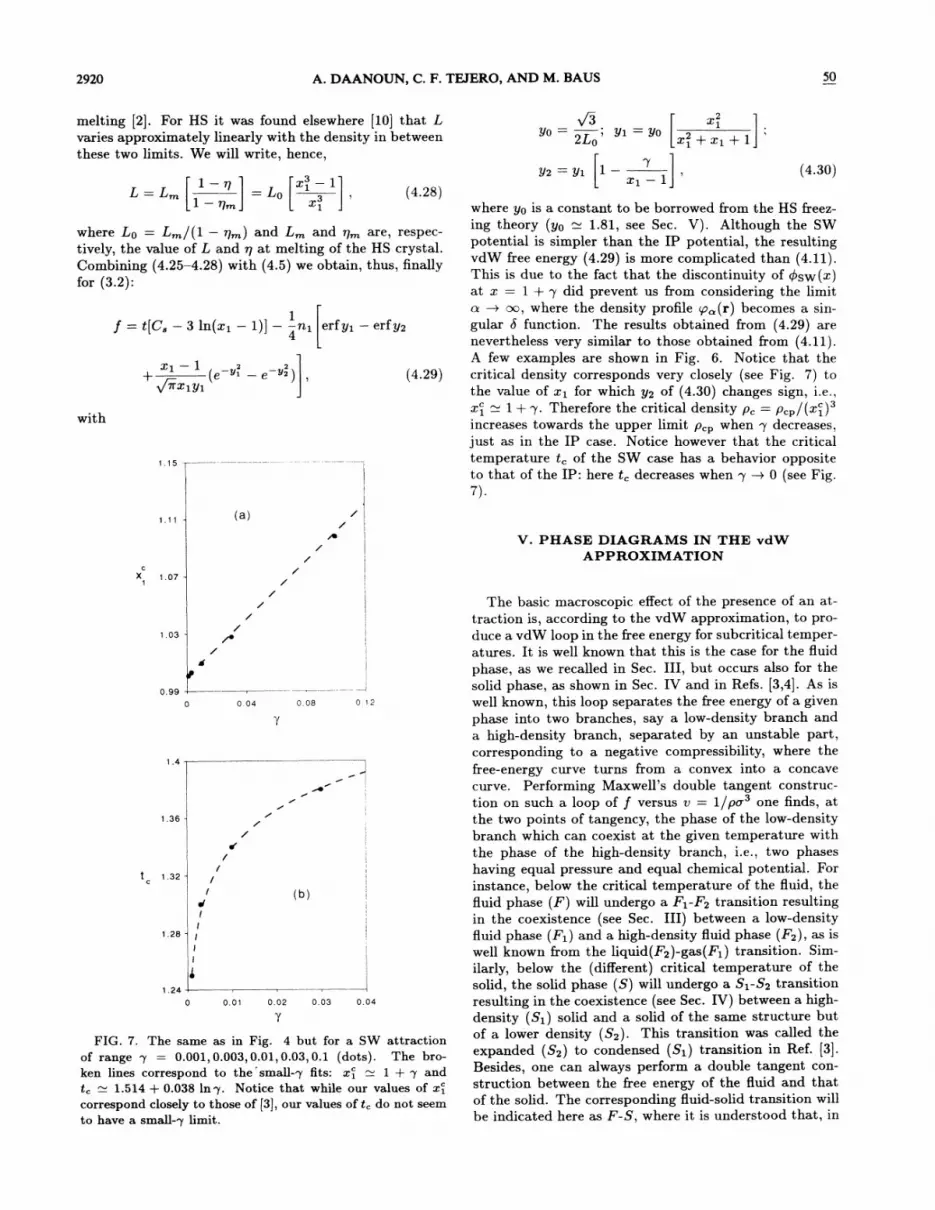
where yp is a constant to be borrowed from the HS freez-ing theory (yo 1.81, see Sec. V). Although the SWpotential is simpler than the IP potential, the resultingvdW free energy (4.29) is more complicated than (4.11).This is due to the fact that the discontinuity of Psw(z)at x = 1+ p did prevent us from considering the limito. m oo, where the density profile p (r) becomes a sin-gular b function. The results obtained from (4.29) arenevertheless very similar to those obtained &om (4.11).A few examples are shown in Fig. 6. Notice that thecritical density corresponds very closely (see Fig. 7) tothe value of zi for which y2 of (4.30) changes sign, i.e. ,

zi = 1+p. Therefore the critical density p, = p,p/(zi)increases towards the upper limit p,~ when p decreases,just as in the IP case. Notice however that the criticaltemperature t, of the SW case has a behavior oppositeto that of the IP: here t, decreases when p m 0 (see Fig.7).

C

X 1.07-1

1.03-

0.990.04

1.4

1.36-

t1.28-

0.01 0.02 0.03 0.04

FIG. 7. The same as in Fig. 4 but for a SW attractionof range p = 0.001,0.003, 0.01,0.03, 0.1 (dots). The bro-ken lines correspond to the'small-7 6ts: x& 1 + p andt, 1.514+ 0.038 lnp. Notice that while our values of 2:&

correspond closely to those of [3], our values of t, do not seemto have a small-p limit.

V. PHASE DIAGRAMS IN THE vdWAPPROXIMATION

The basic macroscopic e8'ect of the presence of an at-traction is, according to the vdW approximation, to pro-duce a vdW loop in the free energy for subcntical temper-atures. It is well known that this is the case for the Quid

phase, as we recalled in Sec. III, but occurs also for thesolid phase, as shown in Sec. IV and in Refs. [3,4]. As is

well known, this loop separates the free energy of a given

phase into two branches, say a low-density branch anda high-density branch, separated by an unstable part,corresponding to a negative compressibility, where thefree-energy curve turns from a convex into a concavecurve. Performing Maxwell's double tangent construc-tion on such a loop of f versus U = 1/pos one finds, atthe two points of tangency, the phase of the low-densitybranch which can coexist at the given temperature withthe phase of the high-density branch, i.e. , two phaseshaving equal pressure and equal chemical potential. Forinstance, below the critical temperature of the Quid, thefluid phase (F) will undergo a Fi F2 transition resu-lting

in the coexistence (see Sec. III) between a low-densityfluid phase (Fi) and a high-density fluid phase (F2), as iswell known from the liquid(F2)-gas(Fi) transition. Sim-

ilarly, below the (different) critical temperature of thesolid, the solid phase (S) will undergo a Si-S2 transitionresulting in the coexistence (see Sec. IV) between a high-

density (Si) solid and a solid of the same structure butof a lower density (S2). This transition was called theexpanded (S2) to condensed (Si) transition in Ref. [3].Besides, one can always perform a double tangent con-struction between the &ee energy of the Buid and thatof the solid. The corresponding Quid-solid transition will

be indicated here as I -S, where it is understood that, in


general, we have F g Fi g F2 and S g Si g S2. Not all

these transitions are thermodynamically stable however.

Only those phases are stable which belong to the convexenvelope constructed with the aid of the four &ee-energybranches (Fi, F2, Si, S2) and the three double tangents(Fi-F2, Si-S2, S F).-A closer inspection of the trian-

gles formed by the three double tangents indicates thatthe competition between the above two vdW loops canonly produce three distinct types of phase diagrams (seeFig. 8). Notice also that for P(z) expressions more com-

plicated than those considered here there could be morethan one vdW loop in the solid &ee energy but we will

not pursue this possibility here and stick to the two cases(2.13,2.14).

Before we can construct the phase diagrams, there re-mains to fix the relative position of the &ee energies. Asseen &om Sec. III, the free energy of the HS Quid dependsonly on the scaled density variable, p/po, where po fixes

the stability limit (0 ( p ( po) of the fiuid. Similarly,in Sec. IV we show that the &ee energy of the HS soliddepends on the scaled density variable, p/p, ~, where p,~fixes the stability limit of the solid (0 ( p ( p,~). When,as before, each phase is taken separately the value of thetwo constants, po and p,~, is immaterial except for the ob-vious geometric restrictions, 7ro po/6 ( 1, vrcr p,~/6 ( 1.When constructing the phase diagram the two phases arerequired and the relative &ee energy depends then on

ln(po/p, ~), which requires that we first fix the value ofthese constants. From the derivation in Sec. IV it is ob-vious that p,p is determined by the value of p at closepacking of the crystal structure considered. For exam-

ple, for a face centered cubic or fcc structure we have

p,~o = ~2 and ni ——12. As to po, the only restrictionis 0.494 & vr poo s/6 ( 1 since we know f'rom the computersimulations [2] that the HS fiuid is stable at least up tothe freezing density xpf ns/6 = 0.494. Here we will fix po

in such a manner that the HS &ee energies, in the absenceof any attraction [P(x) = 0], cross at mpcrs/6 = 0.515 inagreement with the results obtained elsewhere [10]. Thisis seen to imply z poa /6 = 0.5157, i.e., the HS fiuid be-comes unstable shortly after it becomes metastable withrespect to the fcc HS solid. When improved HS equationsof state are used, the HS &ee energies will automaticallycross at this density but notice that one cannot simplyimprove the equation of state of one phase, and keepa simple &ee-volume approximation for the other phasebecause some of these combinations are void of HS &ee-energy crossing. In order to keep the proper HS &ee-energy crossing, one usually will have to improve boththe description of the Quid and of the solid. As long asthe proper HS crossing is guaranteed the results are qual-itatively similar whatever the HS equations of state used.Here we have introduced an po parameter in the descrip-tion of the HS Quid in order to be able to use very simple(free-volume) equations of state, just as in the originalvdW theory, and then chosen the value of n poo /6 to beapproximately 0.52 so as to secure the proper HS freeenergy crossing. Once these constants (po, p,~) are fixed,the phase diagram of the system depends only on therange of the attractions, i.e., the value of p (SW) or 1/n(IP) in (2.13,2.14). Notice that in the particular case of

(a)

S-

(c)

S-1

FIG. 8. To construct the convex envelope of f vs v we

consider the 12 possible triangles formed by the three doubletangents (Fq-Fq, Sq-Sq, and S E) of negative -slope (positivepressure). For only six triangles will the S Fdouble tangent-always belong to the convex envelope. For only three of thesesix triangles do we have that the pressure of the coexistingsolids is larger than the pressure of the coexisting Suids . Thelatter three triangles generate (when changing the tempera-ture) the three types of phase diagrams found. An exampleof each of these three situations is shown in the figure (thedouble tangents belonging to the convex envelope are the full

lines while the dashed lines correspond to metastable coexis-tences). The three cases shown belong to attractions of long

(a), intermediate (b), and short (c) range.

2922 A. DAANOUN, C. F. TEJERO, AND M. BAUS SO

the discontinuous SW attraction we also need the valueof I,o [cf. (4.30)]. For the fcc-HS crystal, we have (see

[2]) I = 0.126 and g = 0.545 x (3y 2/vr) 0.736, andhence I0 0.477.

We now consider, as an illustration, the calculation ofthe phase diagrams, within the present vdW approxima-tion, for the particular case of a SW attraction (2.13),since this is a case for which simulations are available[3]. The two phases considered are, a fluid phase de-scribed by the free energy (3.7) and a fcc crystal describedby the free energy (4.29). For a fcc structure, we have

nq ——12 and n p, &o' /6 = m/3y 2. As explained above,the two inputs are vrpoo /6 = 0.5157 for the fluid andIo ——0.477 for the solid. Using the reduced tempera-ture, t = Ic~T/e, and the reduced pressure, p = pa /e,the phase diagrams will depend only on p, i.e. , the rangeof the SW-attraction relative to the HS repulsion. Inagreement with the other, more rigorous, calculations ofRefs. [3,4] and with the general argument above, we findthree diferent types of phase diagrams. For large p val-

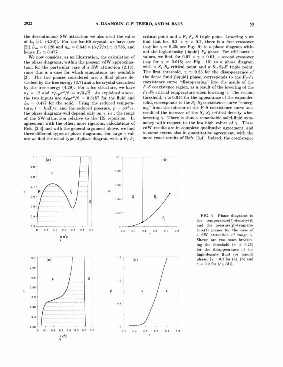
ues we find the usual type of phase diagram with a Fi-F2

critical point and a Fq-F2-S triple point. Lowering p wefind that for, 0.3 ) p ) 0.2, there is a first crossover(say for p 0.25; see Fig. 9) to a phase diagram with-out the high-density (liquid) F2 phase. For still lower pvalues, we find, for 0.02 ) p ) 0.01, a second crossover(say for p 0.015; see Fig. 10) to a phase diagramwith a Si-S2 critical point and a Si-S2-F triple point.The first threshold, p 0.25 for the disappearance ofthe dense Quid (liquid) phase, corresponds to the Fq-F2coexistence curve "disappearing" into the inside of theF-S coexistence region, as a result of the lowering of theFq-F2 critical temperature when lowering p. The secondthreshold, p 0.015 for the appearance of the expandedsolid, corresponds to the Si-S2 coexistence curve "emerg-ing" &om the interior of the F-S coexistence curve as aresult of the increase of the Si-S2 critical density whenlowering p. There is thus a remarkable solid-Quid sym-metry with respect to the low-high values of p. ThesevdW results are in complete qualitative agreement, andto some extent also in quantitative agreement, with themore exact results of Refs. [3,4]. Indeed, the coexistence

(a)0. 1

0.9-

0.8-F

0,08-

0.7- 0.06-

0.6-0.04-

0.5-

0.4

0.3 I I

0 0.1 0.2 0.3 0.4

3KG P6

(c)

0.65

0.5 0.6 0.4 0,5 0.6 0.7 0.8

1,8(d

FIG. 9. Phase diagrams inthe temperature(t)-density(p)and the pressure(p)-tempera-ture(t) planes for the case ofa SW attraction of rangeShown are two cases bracket-ing the threshold (p 0.25)for the disappearance of thehigh-density fluid (or liquid)phase. [p = 0.3 for (a), (b) and

p = 0.2 for (c), (d)].

0.6

0.55

0.5

0.45

0.4

]0.35 I I I I 1

0 0.1 0.2 0.3 0.4 0.5 0.6 0.7 0.3 C.4 0.5 0.6 0.7 0.8


0.8(a)

0.7

0.6 F 6

0.5

0.4p 4

0.32

0.2

0.1

1.7

1.5-

1.3-

0.2 0;4 0.6 0.8

40

30

0.2 0.4 0.6 0.8 FIG. 10. The same as inFig. 9 but for two valuesof p bracketing the threshold

(p 0.015) for the appear-ance of the low-density (or ex-panded) solid phase. [p = 0.02for (a), (b) and p = 0.01 for (c),(d)].

O.9-F S

P 2O

0.7-

0.5- 10

0.1

0.2 0.4 0.6 O.800.5 0.9 1.3 1.7

fE CX P3

6

curves found here are very similar to those of [3,4] whilethe thresholds and critical points are also comparable.Similar results are obtained for the IP attraction: here,the threshold values of n are, 7 & n & 8, for the firstthreshold and, 90 ( n & 100, for the second threshold.

VI. CONCLUSIONS

We have shown that the recent results [3,4] concerningthe eEect of the range of the attractions relative to therange of the repulsions of a simple Quid on its phase di-agram can be semiquantitatively understood in terms ofthe competition of the standard vdW theory of the Quidphase with the alternative [12] but equally simple vdWtheory of the solid-phase introduced above. In particu-lar, we have shown that this competition leads to threediferent types of phase diagrams with a remarkable solid-Buid symmetry. For the case of a square-well attractionof range p it was shown, in agreement with other find-

ings [11,3,4], that the liquid phase disappears as a stablephase for p values below p 0.25, while a new stablesolid phase appears for p values below p 0.015. Asdiscussed elsewhere [13,3,4] such small values of p canperhaps be realized in well-prepared colloidal dispersionswhere the depletion forces due to the added polymer willaccount for the attraction between the colloidal particlesallowing for a simple nuid" description to be used forthis otherwise complex system.

ACKNOWLEDGMENTS

G. F. Tejero acknowledges the DGIGYT (Spain)(PB91-0378) and M. Baus the FNRS (Belgium) and theAssociation Euratom-Etat Beige. M. Baus gratefully ac-knowledges valuable discussions with H. N. W. Lekkerk-erker about the interest of this study for the phase be-havior of colloidal dispersions.


[1] See, e.g. , L. D. Landau and E. M. Lifshitz, StatisticalPhysics, 3rd ed. (Pergamon Press, Oxford, 1989), Sec.76.

[2] J. P. Hansen and I. R. McDonald, Theory of Simple Liquids, 1st ed. (Academic Press, London, 1976).

[3] P. Bolhuis and D. Frenkel, Phys. Rev. Lett. 72, 2211(1994).

[4] C. F. Tejero, A. Daanoun, H. N. W. Lekkerkerker, andM. Baus, Phys. Rev. Lett. 73, 752 (1994).

[5] J. S. Rowlinson, Liquids and Liquid Mixtures (Butter-worths, London, 1959), p. 90.

[6] T. M. Reed and K. E. Gubbins, App/ied Statistica/ Mechanics (Mc Graw-Hill, Tokyo, 1973), p. 282.

[7] R. Hall, J. Chem. Phys. 57, 2252 (1972).[8] J. F. Lutsko and M. Baus, J. Phys. Condens. Matter 3.

[91

[10]'11]

ii 12)

l. 3]

6547 (1991).R. Ohnesorge, H. Lowen, and H. Wagner, EurophysicsLett. 22, 245 (1993).J. F Lutsko and M. Baus, Phys. Rev. A 41, 6647 (1990).A. P. Gast, C. K. Hall, and W. B. Russels 3. ColloidInterface Sci. 96, 251 (1983).An alternative vdW theory for the solid can be found inD. A. Young, J. Chem. Phys. 98, 9819 (1993).The lattervdW theory is inspired by the Buid-phase theory andhence treats the cohesive energy as a phenomenologicalconstant whereas here it is given explicitly in terms ofthe attractive potential P(x) by (4.10).For a recent review see, e.g. , H. N. W. Lekkerkerker, j.K. G. Dhont, H. Verduin, C. Smits, and 3. S. van Duijn-eveldt, Physica A (to be published).

van der waals theory for solids

Documents