1

A methodological roadmap to quantify animal-vectored spatial ecosystem subsidies 1 2 Diego Ellis-Soto1,2+, Kristy M. Ferraro3+, Matteo Rizzuto4, Emily Briggs3,5, Julia D. Monk3, Oswald 3 J. Schmitz3 4 5 1 Department of Ecology and Evolutionary Biology, Yale University, New Haven, CT, USA 6 2 Center for Biodiversity and Global Change, Yale University, New Haven, CT, USA 7 3 School of the Environment, Yale University, 370 Prospect Street, New Haven, CT, USA 8 4 Department of Biology, Memorial University of Newfoundland St. John’s, Canada 9 5 Department of Anthropology, Yale University, New Haven, CT, USA 10 Corresponding author: diego.ellissoto@yale.edu 11 12 + These authors contributed equally to this work 13 14 Keywords: Meta-ecosystem theory, animal movement, biogeochemistry, ecosystem ecology, 16 stoichiometry, remote sensing 17

18

2

Abstract 19 20 Ecosystems are open systems connected through spatial flows of energy, matter, and nutrients. 21 Predicting and managing ecosystem interdependence requires a rigorous quantitative 22 understanding of the drivers and vectors that connect ecosystems across spatio-temporal 23 scales. Animals act as such vectors when they transport nutrients across landscapes in the form 24 of excreta, egesta, and their own bodies. Here, we introduce a methodological roadmap that 25 combines movement, foraging, and ecosystem ecology to study the effects of animal-vectored 26 nutrient transport on meta-ecosystems. The meta-ecosystem concept — the notion that 27 ecosystems are connected in space and time by flows of energy, matter, and organisms across 28 boundaries — provides a theoretical framework on which to base our understanding of animal-29 vectored nutrient transport. However, partly due to its high level of abstraction, there are few 30 empirical tests of meta-ecosystem theory, and while we may label animals as important 31 mediators of ecosystem services, we lack predictive inference of their relative roles and impacts 32 on diverse ecosystems. Recently developed technologies and methods — tracking devices, 33 mechanistic movement models, diet reconstruction techniques and remote sensing — have the 34 potential to facilitate the quantification of animal-vectored nutrient flows and increase the 35 predictive power of meta-ecosystem theory. Understanding the mechanisms by which animals 36 shape ecosystem dynamics may be important for ongoing conservation, rewilding, and 37 restoration initiatives around the world, and for more accurate models of ecosystem nutrient 38 budgets. We provide conceptual examples that show how our proposed integration of 39 methodologies could help investigate ecosystem impacts of animal movement. We conclude by 40 describing practical applications to understanding cross-ecosystem contributions of animals on 41 the move. 42

43

3

Introduction 44 45 Ecosystems and animal nutrient cycling 46 47 Flows of energy, nutrients, matter, and organisms crisscross landscapes worldwide, connecting 48 intrinsically open ecosystems over space and time. The advancement of meta-ecosystem 49 theory (Loreau et al. 2003; Leroux & Loreau 2008; Massol et al. 2011; Marleau et al. 2014) has 50 aided our understanding of the influence of these spatial exchanges in both donor and recipient 51 ecosystem functioning (Gounand et al. 2018b). Classic ecosystem theory holds that the spatial 52 flow of organic and inorganic matter from source to recipient locations is largely passive, coming 53 for example from in situ weathering of parent geological material, release from riverine 54 sediments, wind-born dust, or rain-driven and snowmelt-driven run-off (Chapin et al. 2012). 55 Nevertheless, there is growing appreciation that ecosystems also receive subsidies via animal 56 movement (Vanni, 2002; Atkinson, Capps, Rugenski, & Vanni, 2017; Schmitz et al., 2018; 57 Mcinturf, Pollack, Yang, & Spiegel, 2019). Such movement can result in an influx of new prey or 58 predators to recipient locations, pulses of animal-transported nutrients in dung and urine, or the 59 accumulation of organic matter via decomposition of carcasses deposited in recipient locations 60 (henceforth, animal-vectored subsidies; Earl & Zollner 2017; Mcinturf et al. 2019). Whenever 61 biotic—such as animal-vectored subsidies—or abiotic processes influence the structure and 62 functioning of ecosystems, they are deemed ecosystem controls (Weathers et al. 2012). Theory 63 predicts that animals can exert top-down control on ecosystems via subsidies, the magnitude of 64 which could sometimes be equal to bottom-up (Leroux & Loreau, 2008; Allen & Wesner, 2016). 65 66 Increasingly, migratory populations of large bodied species are recognized for playing an 67 especially important role as landscape-scale vectors of ecosystem subsidies (Bauer & Hoye 68 2014). Yet at the same time, across the globe, their populations are in decline (Wilcove & 69 Wikelski 2008; Dirzo et al. 2014) and their movement is increasingly constrained by human 70 activities (Tucker et al. 2018). The implications of such effects on top-down control over 71 ecosystem functioning at broad spatial scales remain uncertain, but estimates suggest they can 72 be substantial (Doughty et al. 2016). Hence, an important avenue of new research in ecosystem 73 ecology is empirically resolving the relative importance of animal-vectored vs. passive subsides 74 on ecosystem functioning. We are at an opportune scientific and technical juncture to begin 75 synthesizing advances made in disparate fields. 76 77

4

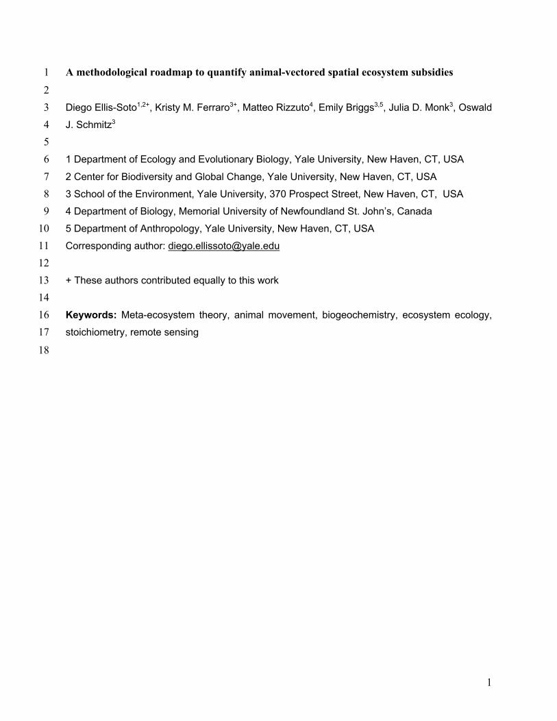
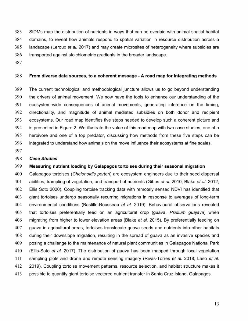
The empirical challenge in understanding and attributing how much control animals exert over 78 ecosystem functioning is to quantify spatial flows of different kinds of animal-vectored subsidies 79 (i.e. excretion, egestion, carcass deposition, reproductive material). While theory is in place to 80 identify the different components that need measuring to obtain a coherent understanding of this 81 phenomenon (Leroux & Loreau, 2008; Earl & Zollner, 2017; Gounand et al. 2018; Schmitz et al., 82 2018), it remains largely conceptual and offers few insights into how to operationalize empirical 83 measurement. Here, we address this limitation by offering a methodological road map that 84 discusses the various measurements that need to be integrated to develop a coherent picture of 85 the quantitative effects of animals on nutrient dynamics across ecosystems. There is now 86 unprecedented ability to characterize functional and structural properties of ecosystems 87 including topography, vegetation community composition, and habitat structure across vast 88 spaces (Bergen et al. 2009; Pettorelli et al. 2018). Likewise, movements of a wide range of 89 animal species can be monitored remotely (Kays, Crofoot, Jetz, & Wikelski, 2015; Wilmers et 90 al., 2015a), which can facilitate quantification of the net effects of animals on nutrient and 91 material transport. New DNA-based and isotopic analyses can resolve dietary nutrient sources. 92 Additionally, these nutrient sources and fates can be mapped spatially using nutrient distribution 93 modeling (West et al. 2010; Sitters et al. 2015; Leroux et al. 2017). While ripe for integration, 94 these methods and technologies continue to be deployed separately in research that examines 95 different components of animal movement and resource use within ecosystems. We show here 96 how these different methods can be used jointly to give a coherent, theory-driven understanding 97 of the ecosystem consequences of animal-vectored nutrient flows across landscapes. 98 99 Materials and Methods 100 101 Meta-ecosystem models to understand animal-vectored subsidies 102 103 The series of measurements we discuss are motivated by ecological theory on meta-ecosystem 104 dynamics. A multitrophic version of such an ecosystem model can be used to consider how 105 internal dynamics of ecosystems are connected by regional flows of materials and organisms 106 between the ecosystems (Marleau et al. 2014). To identify the processes that need to be 107 measured, we consider a model configured as a four trophic level food chain (Fig. 1), which 108 describes the dynamics of a single abiotic nutrient or element (N), a plant (P), a herbivore (H), 109

and a carnivore (C) within and between 𝑖 local ecosystems that together create the meta-110

ecosystem. This structure is intended for simple illustrative purposes to show how to relate the 111

5

dynamical systems model to the salient ecosystem and spatial processes that need to be 112 measured. The model can be made more complex by considering multiple nutrients to make it 113 stoichiometrically explicit (Leroux et al. 2012; Cherif & Loreau 2013) as well as multiple species 114 among trophic levels (McCann et al. 2005). Such granularity is beyond the scope of this paper. 115 Instead, we use this theoretical framework specifically to identify salient processes (and inherent 116 variables) that need to be measured to obtain a quantitative understanding the role of animals in 117 connecting and shaping the structure and functioning of local ecosystems across spatial scales. 118 The model reveals two salient processes that need to be considered: trophic interactions and 119 nutrient translocation and deposition. These two processes can be subdivided into five more 120 finely resolvable spatial components (Fig.1) that require detailed measurement. Hence, our 121 roadmap focuses on measuring these five components. 122 123 Trophic interactions within ecosystem 𝑖 determine nutrient uptake and assimilation by 124 herbivores and carnivores (Fig. 1) that may vary in size, and habitat structure within an 125 ecosystem determines species spatial occurrences and the nature of their interactions (Schmitz 126 et al. 2017). Thus, an accounting of animal spatial interactions will require analysis of: (1) the 127 spatial extent and spatial grain size for analysis of the focal animal species and their 128 interdependent predators or prey/resources (i.e., spatial trophic food chain structure) in relation 129 to (2) the habitat structure within and between source and recipient local ecosystems. Moreover, 130 animals can be selective in their choice of resources, necessitating further spatial analyses of 131 (3) the resources selected by animals in source and recipient locations. Nutrient translocation 132 and deposition in ecosystems will depend on (4) the movement rates and directional spatial 133 flows of animal species and animal-vectored nutrients, and (5) the amounts and spatial 134 deposition rate of animal transported nutrients or materials, which can include the animals’ own 135 body mass, waste products, reproductive material, and dispatched prey. Each of these 136 components can be measured with its own set of technologies (Fig. 2). We next provide a brief 137 review of these tools and of their potential use in the context of measuring animal-vectored 138 subsidies. 139 140 (1) Spatial trophic structure 141 The first step to understanding how animal movement shapes ecosystems is to describe the 142 geographic domain over which focal animals roam and their trophic position within food chains, 143 including the scope of interactions with predators and resources (Fig. 2). These factors will 144 determine the geographic area and spatial grain of interest, the animals’ habitat domain within 145

6

that area, and any ecosystem effects the animal could have within said domain through 146 cascading impacts on associated food webs. The habitat domain is the spatial extent of habitat 147 space used within a species’ broader home range that is relevant to interspecific interactions, 148 e.g., areas used for foraging or avoiding predation (Schmitz et al. 2017). 149 150 Characterizing the spatial grains at which animals interact with other species and their 151 environment is crucial to understanding their distributions. Animal movement can be described 152 at fine spatial scales (e.g. responses to environmental resources such as foraging [see section 153 3]) or at coarser scales, such as their broad home range (introduced in section 4) (Mertes et al. 154 2020). Fine and coarse spatial grains have been termed “response grain” and “occupancy 155 grains”, respectively (Mertes et al. 2020). To quantify an animal’s response grain, first passage 156 time analysis can be employed. These are defined as the time it takes an animal to cross a 157 circle with a defined radius -- and as such scale dependent -- and can quantify the time duration 158 of an individual animal present within such a circle (Fauchald & Tveraa 2003). First passage 159 time allows estimating the spatial scale at which an individual animal focuses its search efforts 160 (i.e. by plotting variance in first passage time against the spatial scale, Fauchald & Tveraa 2003, 161 Fig. 2 bottom left panel). As such, hierarchical scales of animal habitat selection (Johnson 1980; 162 Mertes & Jetz 2017; Mertes et al. 2020) should drive the spatial resolution of remote sensing 163 products selected for analysis, not the other way around. This is especially relevant for animal 164 movement data, which are typically measured at finer spatio-temporal resolutions than data 165 from remotely sensed imagery (Remelgado et al. 2017, 2019). The habitat domain can be 166 measured using movement data by tracked individuals across a landscape, to calculate an 167 animals utilization distribution and probabilities of spatial locations associated with foraging and 168 migration behaviour across a landscape (Schmitz et al. 2017). A three-dimensional utilization 169 distribution could be estimated if vertical movements are tracked, e.g. movement in forest 170 canopies (McLean et al. 2016). 171 172 Species interactions can alter animal movement behaviour, which can in turn impact ecosystem 173 nutrient dynamics (Schmitz, Hawlena, & Trussell, 2010; Schmitz et al., 2018). Hence 174 consideration of the amount and spatial domain of animal vectored subsidies needs to consider 175 species embeddedness within food chains. Moreover, such consideration will enhance the 176 appreciation that animal vectored subsidies can trigger the rearrangement of food chains or 177 initiate novel trophic interactions (Montagano et al. 2019). Generally in this context, primary 178 producers have a trophic position of 1, primary consumers have a trophic position of 2, 179

7

secondary consumers have a trophic position of 3, and so on (Leroux & Loreau 2012). Yet there 180 are many animals that occupy trophic positions between these discrete designations. For 181 example, an omnivore may consume mostly primary consumers, but also some secondary 182 consumers and therefore have a trophic position between 2 and 3 (Kelson et al 2020). We 183 discuss how stable isotopes may be used to determine trophic position in section 3, which is 184 important to resolve the nature and source of nutrients (e.g. largely plant-based vs. largely 185 animal-based) that comprise subsidies (see section 3, Kelson et al. 2020). 186

187 (2) Habitat structure within and between source and recipient locations 188 189 Habitat structure and topographic features, within and between source and recipient locations, 190 shape animal movement and nutrient transport within habitat domains (Leroux & Loreau, 2008; 191 Gounand, Little, Harvey, & Altermatt, 2018; Schmitz et al., 2018). A spatially accurate 192 characterization of these fundamental ecosystem attributes is key to understanding why, how, 193 and where animals move over the landscape (Fig. 2). Earth observation via satellite, airborne, 194 or drone imagery provides an important basis for developing such a characterization (Allan et al. 195 2018; Pettorelli et al. 2018). Remotely sensed landcover maps (i.e. forest, grassland, urban) can 196 be used to delineate ecosystem boundaries and assess how these change through time. 197 Advances of LiDAR (Light Detection and Ranging) make it possible to characterize vertical 198 habitat structure and above-ground vegetation biomass within and across ecosystem 199 boundaries. Furthermore, ecosystem productivity can be remotely measured and represented 200 as vegetation indices (de Araujo Barbosa et al. 2015; Pettorelli et al. 2018). Topographic 201 products, such as slope and topographic ruggedness (Amatulli et al. 2018), can resolve passive 202 abiotic flow pathways to pinpoint where nutrients may end up on the landscape (e.g., flow down 203 concave and into convex surfaces; Lindeman, 1942; Leroux & Loreau, 2008). Finally, LiDAR 204 estimates are becoming available from the Global Ecosystem Dynamics Investigation (GEDI) 205 mounted on the International Space Station, which measures forest structure and above-ground 206 biomass density across the globe (Hancock et al. 2019) 207 208 More finely resolved structure can be obtained within habitats using hyperspectral technologies 209 to collect hundreds of bands across the electromagnetic spectrum which distinguish unique 210 ‘fingerprints’, referred to as spectral signatures for different kind of environmental features 211 (Stuart et al. 2019). Such spectral signatures can be related to spatial patterns in plant 212 functional diversity, vegetation elemental composition, and plant density (Knyazikhin et al. 2013; 213

8

Jetz et al. 2016; Schneider et al. 2017; Durán et al. 2019). Further, endmember extraction from 214 multispectral imagery can be used to extract information on subpixel features, e.g., to identify 215 signatures of water availability and abundance (Xie et al. 2016) . 216 217 Remotely sensed environmental products have different pixel resolution, commonly referred to 218 as ‘grain size’. Accessing and utilizing a plethora of remote sensing products is facilitated 219 through geoprocessing tools such as Google Earth Engine, the Movebank Env-Data system, 220 and the getspatialdata package (Pettorelli et al. 2014; Clark et al. 2016; Wegmann 2017). We 221 list a collection of remote sensing products available to study ecosystem features across source 222 and recipient locations in Table 1. Regardless of the product used, coherent understanding 223 requires a grain size that aligns with the grain size of measurement of animal movement. 224 225 (3) Resources available to and selected by animals in source and recipient locations 226 227 Characterization of species habitat domains and structure can next be used to determine why 228 animals move where they do, and what resources they use in source and recipient locations 229 (Fig. 2). This can be accomplished using resource selection functions (RSF; Boyce et al. 2002) 230 and step selection functions (SSF; Fortin et al. 2005). Generally, these functions associate 231 environmental variables with locations used by individual animals and compare these with 232 randomly generated points representing locations available to, but not used by, them (Michelot 233 et al. 2019). Both methods estimate the probability of animal presence as a function of 234 environmental covariates. SSF can be used further to predict future movement paths of animals, 235 while RSF predicts spatial patterns of species occurrences over spatio-temporal scales 236 (Michelot et al. 2019). Parameters from SSF can highlight whether animals avoid or are 237 attracted to certain landscape features or resources. For example, SSF analysis reveals that in 238 Etosha National Park, Namibia, elephants avoided areas with high tree biomass and were 239 attracted to water sources and grassland patches with long term patterns of productivity 240 (Tsalyuk et al. 2019). This could indicate that waterholes and grasslands receive more animal-241 vectored subsidies from elephants when compared to steep areas or dense forests. Such 242 behavioural information would improve mechanistic predictions of nutrient redistribution by 243 these wide-ranging megafauna which are known to play a large effect on regional carbon 244 budgets (Berzaghi et al. 2018). 245 246

9

Resource selection is a hierarchical process (Courbin et al. 2013). While RSF and SSF are 247 broad-scale measures of animal movement and habitat use, more finely resolved measures are 248 needed to understand which food items are used by animals and their nutritional values within 249 different locations. This understanding of animal food consumption and eventual processing and 250 deposition (in body material, or as urine and fecal matter) can provide an understanding of 251 where and how nutrients removed from donor ecosystems end up in recipient ecosystems. 252 Additionally, the identity of consumed resources directly impacts the quantity and quality of 253 nutrients deposited by animals (Subalusky & Post 2018). 254 255 Traditionally, dietary analyses have been performed based on physical dissection and 256 microhistological analyses of stomach contents and fecal matter (Holechek et al., 1982, Joly, 257 2018). These methods, however, often require either opportunistic sampling of carcasses or 258 destructive harvesting of live animals. DNA-metabarcoding provides an alternative, as it allows 259 for the identification of materials consumed using fecal matter alone (Kartzinel et al. 2015; see 260 Deagle et al., 2019 for an overview of DNA-metabarcoding methods). DNA-metabarcoding can 261 shed important insights into the trophic ecology of source and recipient sites, and how 262 consumption, and thus acquisition and transport of nutrients, can change in time and space 263 (Pansu et al. 2019). For example, Atkins et al. (2019) combined GPS tracking data of bushbuck 264 (Tragelaphus sylvaticus) with DNA-metabarcoding of fecal samples to show that herbivores 265 occupy new habitats and forage on novel food items after extirpation of their predators. 266 Bushbuck presence further changed plant community composition (demonstrated by comparing 267 plant composition in exclosure and control plots) (Atkins et al. 2019). A playback experiment of 268 predator sounds was able to revert bushbuck behaviour as they perceived predation risk (Atkins 269 et al. 2019). 270 271 Stable isotopes, such as δ15N, δ13C, and δ18O, are also powerful tools in elucidating the trophic 272 position (Ben-David et al., 2012), diet, and foraging location of a focal species in a non-invasive 273 manner (Newsome et al. 2010; Kristensen et al. 2011). In general animals are enriched by ~3‰ 274 of nitrogen and ~1‰ of carbon compared to what they eat, providing an estimate of trophic 275 position (Post 2002). Therefore, trophic position can be discerned by using the isotopic 276 signature (i.e. δ15N) of the consumer, of the ecosystem’s primary producers, and a 277 discrimination factor for the change in δ15N enrichment between the ecosystem’s trophic levels 278 (Kelson et al. 2020). Using stable isotopes could also be a cost-effective way to identify the 279 correct primers when conducting DNA-metabarcoding. For example, while white-tailed deer are 280

10

primarily herbivores, there is some evidence that they sometimes consume animal matter (Ellis-281 Felege et al. 2008). If stable isotopes revealed that deer have an omnivorous diet, DNA-282 metabarcoding could be used to discern exactly what animal material they consumed. 283 284 Stable isotopes can also be used to arrive at approximate estimates of diet. The isotopic 285 signatures of food items (for example, C3 and C4 plants) often vary from one another. 286 Therefore, examining the isotopic signature in bone, tooth, or feces has shown a successful 287 method of coarsely understanding diet (Ben-David & Flaherty 2012). We recommend using 288 stable isotopes to determine diet if DNA-metabarcoding is not financially possible, when using 289 samples that have degraded and DNA-metabarcoding is no longer possible, or when a broad 290 understanding of diet is sufficient for the question at hand For an extensive overview of using 291 stable isotopes for ecological research, see Ben-David & Flaherty (2012), Hobson et al., (2019), 292 and West et al. (2010). 293 294 (4) The movement rates and directional patterns of animal species and subsequently 295 translocated nutrients 296 297 Animals can transport nutrients along and against biophysical gradients (Earl & Zollner, 2017; 298 Mcinturf et al., 2019). Therefore, an understanding of animal movements will elucidate the 299 nature and scale of consequent nutrient transfer (Fig. 2). Patterns of animal movement are 300 directly related to the degree of connectivity (cij, Fig. 1) among local ecosystems as well as the 301 movement rates of the animals (dH, dC, Fig. 1), which depend on the topography of the 302 biophysical gradient. Advances in animal tracking technologies – dubbed biologging – offer 303 possibilities to study internal (e.g., physiology, metabolism, reproduction) and external (e.g., 304 social, environmental) drivers of animal movement (Nathan et al. 2008). Biologging enables 305 quantification of the space-use and resource requirements of animals (Kays et al. 2015; Hays et 306 al. 2019). The frequency with which animals visit certain areas (e.g., waterholes, fruit bearing 307 tree, latrines) can be estimated via first passage times and recursive analysis (Mahoney & 308 Young 2017; Bracis et al. 2018; Mertes et al. 2020). 309 310 Migrations are among the greatest examples of animal movement. Extensive research has 311 explored their direction, length, and drivers (Dechmann et al. 2017; Somveille et al. 2018, 2019). 312 Locations of an animal’s track can be classified into specific movement strategies (i.e. disperser, 313 migrator, nomad, central place forager) by segmentation methods (Bastille-Rousseau et al. 314

11

2016; Edelhoff et al. 2016), thus setting the stage for further analysis. Fine-scale animal 315 behaviour (i.e. foraging, rest, travel) can be resolved in GPS data using behavioural change 316 point analysis, expected-maximum binary clustering methods (Garriga et al. 2016), and state-317 space models (Patterson et al. 2008). A promising approach combining state-space and 318 continuous time correlated random walk models (Michelot & Blackwell 2019) allows estimating 319 behavioural states when using tracking data that are not sampled at regular time intervals, 320 which is a common occurrence with biologging data. 321 322 Modern biologging tags are comprised of GPS units, accelerometers, and additional on-board 323 sensors. Accelerometers estimate change in velocity of body postures over time and can 324 classify behavioural states of wild animals, including hunting, killing, resting (Brown et al. 2013; 325 Williams et al. 2014), and even scent marking (Bidder et al. 2020). Accelerometers also allow 326 quantifying energy expenditure of animals and of specific behaviours. Common methods for 327 such energy expenditure are two closely linked metrics; Overall Dynamic Body acceleration 328 (ODBA) and Vectorized sum of the Dynamic Body Acceleration (VeDBA) (Wilson et al. 2006, 329 2020). We refer to Joo, Boone, Clay, & Patrick, (2019) for a review on animal movement 330 analysis. 331 332 Movement ecology increasingly studies fine scale behaviours such as foraging or sociality 333 (Strandburg-Peshkin et al. 2015; Bennison et al. 2018) that can determine fine scale spatial 334 heterogeneity in nutrient release, a process not yet considered in the current literature on 335 animal-vectored subsidies (Gounand et al. 2018b). At the same time, movement ecology rarely 336 quantifies the scale, scope, and magnitude of animal-mediated nutrient transfers. 337

338 (5) The amounts and deposition rate of animal transported nutrients or material 339 340 Remote sensing offers quantitative measures of ecosystem structure at broad geographic 341 scales. Collecting environmental data in the field provides detailed information that is essential 342 and complementary to remote sensing to understand how local microclimate influences 343 ecosystem dynamics and the distribution of animals and the resources they consume 344 (Zellweger et al. 2018) (Fig. 2, right panel). Local observations identify how trophic interactions 345 and community structure vary across habitats and environmental gradients. For example, one 346 could measure a site’s microtopography (slope, elevation, roughness), surrounding vegetation 347 type and cover. The development of methods to account for such micro-environmental variation 348

12

is necessary to facilitate realistic representations of environmental conditions experienced by 349 organisms. Downscaled remote sensing products show promise in providing such fine spatial 350 detail (Maclean et al. 2019; Maclean 2020) and, once overlaid with animal locations, enable 351 identification of habitats that are source and recipient locations for animal-vectored nutrient 352 subsidies. 353 354 Animal vectored subsidies involve several processes, including consumption, excretion, 355 egestion, and deposition of carcasses and parturition material (McSherry & Ritchie 2013; 356 Subalusky & Post 2018; Wenger et al. 2019). For example in the Maasai Mara National Park 357 Reserve, Kenya, every day Hippopotamus egest approximately 36 tons of wet biomass 358 consumed in terrestrial ecosystems into the Mara river, approximately 15 % of the dissolved 359 organic carbon loading from the upstream catchment (Subalusky et al. 2015). Also in the Mara, 360 mass drowning of wildebeest contributes ~18% of the total dissolved organic carbon to the river 361 ecosystem (Subalusky et al. 2017). 362 363 Standard biogeochemical methods, which include analyses that quantify elemental composition 364 of materials, can be used to characterize the stoichiometry and total nutritional composition of 365 food items (Vanni et al., 2002). Additionally, these methods can assess nutrient quality and 366 quantity of animal-deposited material (e.g. egesta, excreta, carcasses) as well as the magnitude 367 of nutrient influx into the surrounding environment through in situ measurement of various soil 368 and plant properties (e.g., pH, soil texture, plant community composition, soil and plant nutrient 369 content) at sites of animal activity (i.e. see Bump et al., 2009, Risch et al. 2020). Finally, given 370 that stable isotope that come from animal tissues and excreta are isotopically enriched 371 compared to their diet, enriched plant and soil materials surrounding the deposition can indicate 372 deposition and use of animal-vectorized subsidies (Bump et al 2009a). Such enrichment may 373 also help parse out passive from active subsidy input. 374 375

The tracing and mapping of spatial nutrient flows and deposition can be aided by using 376 stoichiometric distribution models (StDMs). Such models predict the geospatial distribution of 377 nutrients in forage items (Leroux et al. 2017). Similar to a species distribution model and point 378 Poisson process models, a resource – in this case a forage item’s nutrient content, either 379 absolute (g/m2; i.e. quantity) or relative (carbon:nitrogen ratio; i.e. quality) – can be defined as 380 the abundance of a given nutrient (nitrogen, phosphorus or carbon) in location xi which is 381 predicted by a vector of environmental covariates z(xi), their coefficients βi, and an error term Ɛ. 382

13

StDMs map the distribution of nutrients in ways that can be overlaid with animal spatial habitat 383 domains, to reveal how animals respond to spatial variation in resource distribution across a 384 landscape (Leroux et al. 2017) and may create microsites of heterogeneity where subsidies are 385 transported against stoichiometric gradients in the broader landscape. 386 387

From diverse data sources, to a coherent message - A road map for integrating methods 388

The current technological and methodological juncture allows us to go beyond understanding 389 the drivers of animal movement. We now have the tools to enhance our understanding of the 390 ecosystem-wide consequences of animal movements, generating inference on the timing, 391 directionality, and magnitude of animal mediated subsidies on both donor and recipient 392 ecosystems. Our road map identifies five steps needed to develop such a coherent picture and 393 is presented in Figure 2. We illustrate the value of this road map with two case studies, one of a 394 herbivore and one of a top predator, discussing how methods from these five steps can be 395 integrated to understand how animals on the move influence their ecosystems at fine scales. 396 397 Case Studies 398 Measuring nutrient loading by Galapagos tortoises during their seasonal migration 399 Galapagos tortoises (Chelonoidis porteri) are ecosystem engineers due to their seed dispersal 400 abilities, trampling of vegetation, and transport of nutrients (Gibbs et al. 2010; Blake et al. 2012; 401 Ellis Soto 2020). Coupling tortoise tracking data with remotely sensed NDVI has identified that 402 giant tortoises undergo seasonally recurring migrations in response to averages of long-term 403 environmental conditions (Bastille-Rousseau et al. 2019). Behavioural observations revealed 404 that tortoises preferentially feed on an agricultural crop (guava, Psidium guajava) when 405 migrating from higher to lower elevation areas (Blake et al. 2015). By preferentially feeding on 406 guava in agricultural areas, tortoises translocate guava seeds and nutrients into other habitats 407 during their downslope migration, resulting in the spread of guava as an invasive species and 408 posing a challenge to the maintenance of natural plant communities in Galapagos National Park 409 (Ellis-Soto et al. 2017). The distribution of guava has been mapped through local vegetation 410 sampling plots and drone and remote sensing imagery (Rivas-Torres et al. 2018; Laso et al. 411 2019). Coupling tortoise movement patterns, resource selection, and habitat structure makes it 412 possible to quantify giant tortoise vectored nutrient transfer in Santa Cruz Island, Galapagos. 413

14

Santa Cruz Island shows a distinct zonation of vegetation. Dry xerothermic plants dominate the 414 low elevations of the national park, with rainfall and the presence of introduced species (e.g., 415 guava) increasing with elevation (Itow 2003). During their downslope migration, adult tortoises 416 can migrate from agricultural areas at higher elevations into the lowlands of the Galapagos 417 National Park (identified through net square displacement, Suppl. Material 1). Overlapping 418 home ranges (Winner et al. 2018) of tagged tortoises located in the lowlands inside the national 419 park can reveal core areas of tortoise utilization distributions, providing a picture of spatial 420 trophic structure. Using this core area, a stratified sampling of surrounding vegetation, soil 421 samples, and description of microtopography can help understand nutrient composition, 422 microbial activity and abiotic properties of selected areas in an attempt to further characterize 423 habitat structure. Such measurements could be compared with samples obtained in areas 424 where tortoises are absent, serving as a control plot (i.e. via exclosures or randomly selecting 425 points outside the tortoise core area) to further isolate animal impacts on biogeochemical cycles 426 and ecosystem fluxes. 427

Given their different photosynthetic pathways (C3 and CAM, respectively) guava likely contains 428 a different isotopic signature (Sage & Zhu 2011) than the tortoises’ most-consumed xerothermic 429 plant at lower elevations of the National Park, the Opuntia echios cacti. Thus, stable isotope 430 analysis of fecal matter containing guava could disentangle contributions by tortoises during 431 their migrations from a donor ecosystem (agricultural areas) to a recipient ecosystem (lowlands 432 of the Galapagos National Park) and make spatially explicit predictions of this animal-vectored 433 nutrient flux. Finally, all of these measures can be combined to develop a nutrient budget for the 434 lowland ecosystem of the Galapagos National Park and include the downslope migration of C. 435 porteri as the mechanism for vectored subsidy (Fig. 3, Fig. 4). Such nutrient ecosystem budgets 436 often attempt to quantify the flows of nutrients through different pools providing an 437 understanding of how these flows may impact ecosystem functioning (Loreau & Holt 2004). 438 Coupling an assessment of nutrient loading with past and present tortoise population numbers 439 could provide a baseline for ongoing conservation initiatives aimed at restoring degraded island 440 habitats by reintroducing giant tortoises to act as ecosystem engineers (Gibbs et al. 2010; 441 Hunter et al. 2020). We provide the necessary code to replicate steps detailed in this conceptual 442 tortoise example (Suppl. Material 1). 443

Quantifying how Canis lupus creates landscape heterogeneity through prey hunting and 444 killing 445 446

15

Predators can have profound cascading impacts on ecosystem nutrient dynamics mediated by 447 their effects on prey mortality and space use (Fig. 5). For example, the hunting behaviour of 448 wolves (Canis lupus) and the subsequent deposition of prey carcasses may create nutrient 449 hotspots across a landscape, creating heterogeneity in nutrient distribution as carcasses 450 decompose at sites with high rates of predation (Bump et al. 2009a; Joseph et al. 2009). To 451 explore this, a recursive analysis (Bracis et al. 2018) based on how often animals return to 452 specific landscape areas defined by a determined circular radii — which could be chosen based 453 on grain sizes identified from First Passage Times (Mertes et al. 2020) — display where and 454 how collared wolves revisit areas in their range. Coupling accelerometer and animal location 455 data can identify hunting, eating, and killing by predators in the wild through behavioural 456 classification and ground-truthing GPS clusters at presumed kill sites (Williams et al. 2014; 457 Wang et al. 2015). These methodologies can pinpoint the exact coordinates and time of hunting 458 and killing events and therefore quantify the movement of the nutrients through these 459 processes. Once a carcass’s presence is identified, camera traps can provide insight into how 460 the predation behaviours of top predators may have cascading impacts on subsidizing 461 scavengers and invertebrates (Perrig et al. 2017; Cunningham et al. 2018). 462 463 Using a stratified sampling scheme of plant and soil characteristics, it is also possible to quantify 464 the nutrients deposited by the carcasses, explore the spatial diffusion of those nutrients, and 465 estimate how long those nutrients stay in the local system before leaching away or being 466 scavenged. These sites can be compared to measurements collected in randomly selected 467 points, which may serve as a control treatment. Assessing the plant community composition and 468 cover will help identify whether killing behaviour of predators leads to changes in plant 469 composition, while soil samples collected below carcasses can be used to compare microbial 470 activity and nutrient availability between carcass and control sites (Metcalf et al. 2016; Risch et 471 al. 2020). Both total soil and plant nutrient concentration as well as enriched δ15N in plant and 472 soil samples can be used to identify and quantify the impact of this animal vectorized subsidy 473 (Bump et al. 2009b; Holtgrieve et al. 2009; Barton et al. 2016). This conceptual study design 474 highlights how predators could concentrate nutrients at kill sites, contributing to landscape 475 heterogeneity with potential knock-on effects on scavenger and plant community distribution. 476 Such knowledge is key for understanding the ecosystem consequences of predator loss (Ripple 477 et al. 2014). 478 479 Moving forward: Future Directions 480

16

481 We have illustrated how individual studies may productively integrate disparate fields and tools 482 to address specific questions about animal-vectored nutrient subsidies within a study system. 483 These disciplines and methodologies can be united to address larger questions about animals 484 and nutrient transport in diverse systems and at multiple scales. Below, we identify the next 485 frontiers in ecological research, which can be resolved through synergistic research linking 486 animal movement and nutrient transport. 487 488 Improve tracing and mapping of animal vectorized subsidies 489 490 We see opportunities to improve predictions of animal vectored subsidies based on advances of 491 Species Distribution Modeling (SDM) such as incorporating a priori expert knowledge (Merow et 492 al. 2016) and joint species distribution modeling (jSDM) (Pollock et al. 2014). Such expert 493 knowledge can represent species geographic ranges or species specific elevational ranges as 494 known from field guides. Expert knowledge could enter StDM’s in the form of a statistical offset 495 which has been shown to improve model predictions from SDM’s (Ellis-Soto et al. n.d.; Merow 496 et al. 2016). Such offset is independent of the predictor variable (nutrient quantity or quality) and 497 would provide a priori expectations of how resources are distributed across a study region 498 rather than assuming an equal likelihood for each cell in a landscape. StDMs could also 499 incorporate soil nutrient maps derived from coarse scale remote sensing (soilgrids database) as 500 an offset reflecting the a priori expectation of a nutrient concentration in a cell. We refer to 501 Merow, Wilson, & Jetz, (2017) for specifics about deploying offsets in logistic regression, but the 502 motivation is that expert information can provide estimates that are complementary to point 503 estimates that could predict nutrient quantity (g/m2) or nutrient ratios (C:N). 504 505 jSDMs predict spatial occurrences of entire communities of species, rather than distributions of 506 single species, as in SDM (Pollock et al. 2014). StDMs could be similarly extended to consider 507 the distribution of multiple individual nutrients (not just their ratios). Particularly, we see potential 508 in adapting jSDM developments from Generalized joint attribute modelling (Clark et al. 2017), 509 Bayesian Ordination and Regression Analysis of Multivariate Abundance Data (Hui 2016), and 510 Spatial factor analysis (Thorson et al. 2015) to develop joint StDM. Such jStDM could be 511 overlapped with autocorrelated kernel density estimators (Fleming et al. 2015) to investigate 512 how animal space use relates to spatial stoichiometry. 513 514

17

We see potential in building upon mechanistic models of animal movement and seed and 515 nutrient dispersal to map the distribution and magnitude of animal vectored subsidies (Bampoh 516 et al. 2019; Kleyheeg et al. 2019; van Toor et al. 2019). These models couple animal movement 517 and gut retention with remotely sensed land cover information to create spatially explicit maps of 518 nutrient dispersal. Such models have provided insights about how extinct and extant animals 519 have influenced nutrient translocations at coarse spatial scales across the globe (Doughty et al. 520 2016; Doughty 2017). These estimates could be refined by incorporating movement models 521 such as allometric random walks (Hirt et al. 2018) and individual based movement models 522 (Bampoh et al. 2019), rather than coarser lateral diffusion movement models which have 523 hitherto been used. 524 525 Estimating animal-mediated nutrient translocation within a home range 526 527 Core areas where individuals within groups or populations might have strongest animal-528 vectorized subsidies effects can be identified using home range overlap indices between 529 individuals. Such overlap indices may be simple convex hulls around individual home ranges to 530 describe population ranges or more sophisticated utilization distributions based on bias-531 corrected Bhattacharyya coefficient as shown by Winner et al., (2018). RSFs of individuals with 532 overlapping home ranges could reflect how these animals utilize resources across long-term 533 timescales. 534 535 Behavioural pattern identification could characterize a suite of animal behaviours within home 536 ranges (e.g., forage, rest, fight, prey capture; Kie et al. 2010) to identify how animals transport 537 nutrients at shorter timescales (Fig. 3). Revisitation and accelerometer analysis hold promise to 538 identify feeding sites, scent marking sites or latrines (Bracis et al. 2018; Bidder et al. 2020). High 539 urine concentration at latrines could influence plant communities, soil nutrient loads, and 540 microbial communities, constituting a nutrient hotspot. Other methods estimate nest locations 541 and reproductive output from telemetry data (Picardi et al. 2019; Bidder et al. 2020). Such 542 behavioural identification can identify where animals assimilate or excrete resources and under 543 which conditions animals act as nutrient sources (bring more nutrients in than they consume, 544 i.e. high urine concentration at latrines or high offspring mortality at nests) or sinks (have a 545 negative net effect on nutrient concentrations at the site). Calculating integrated step selection 546 functions (Avgar et al. 2016) using exclusively animal locations that were associated with 547 foraging behaviour (Nathan et al. 2012) could identify such nutrient sources. Habitat selection 548

18

could be explored at fine detail by using drones to create study-site specific landcover maps 549 (Strandburg-Peshkin et al. 2017). 550 551 Animal-vectored subsidies in the Anthropocene 552 553 In human-modified landscapes, animals find themselves crossing a matrix of fragmented 554 habitats and human pressures (i.e. population density, infrastructure and agricultural areas) that 555 vary in permeability. Human modification of landscapes, such as urban development of roads or 556 C4 plant monocultures for agriculture, can alter diet and nutrient transfer by animals (Magioli et 557 al. 2019). For example, Roe deer (Capreolus capreolus) in central France routinely act as 558 vectors for large quantities of artificially-introduced nitrogen, which they obtain by foraging in 559 agricultural areas, which are deposited near resting sites in forested areas (Abbas et al. 2012). 560 In New Mexico, USA, snow geese (Chen caerulescens) perform daily foraging trips from wildlife 561 refuges to agricultural areas to feed on corn and alfalfa. This nutrient translocation was shown 562 to increase phosphorous nutrient loadings up to 75% in wetland ponds (Kitchell et al. 1999). 563 Thus, animals can link natural areas with human modified landscapes and modify the nutrient 564 budgets of ecosystems. 565

Mechanistic models of animal vectored subsidies (Bampoh et al. 2019) could predict 566 how nutrient budgets of ecosystems are altered by the removal of species, such as large bodied 567 animals (Bello et al. 2015; Sobral et al. 2017), or specific individuals (i.e. elephant bulls in 568 Kruger National Park (Davies & Asner 2019)), or animal introductions (goat introduction in the 569 Galapagos (Bastille-Rousseau et al. 2017)). These models could identify causal links between 570 ecosystem functioning and animal mediated subsidies. Such knowledge would provide evidence 571 to rewilding initiatives aiming to restore lost ecosystem services through animal reintroductions 572 (Falcon Wilfredo & Hansen 2018; Lundgren et al. 2018). 573 574 Conclusion 575 576 Understanding how animals move through both natural and human dominated landscapes to 577 influence ecosystem properties and functions is in need of concerted analysis. To this end, we 578 have provided a methodological road map that draws together methods of analysis across 579 disciplinary fields. We show how, when combined, these can lead to integrative, coherent 580 understanding of how animal vectored subsidies drive spatial ecosystem structure and 581 functioning. It is through the integration and collaboration of disciplines that we can address and 582

19

understand the importance of this type of nutrient transport in a spatially explicit manner. We 583 hope that the introduced methodological roadmap will facilitate empirical studies that quantify 584 how much the fluxes of nutrients from one pool to another across landscapes can be attributed 585 to animal-vectored subsidies. 586 587 Acknowledgments: We thank Kevin Winner, Brett Jesmer, Ruth Yvonne Oliver and Nathalie 588 Sommers for helpful feedback on this publication. We further appreciate support from Stephen 589 Blake, Fredy Cabrera, Sharon Deem, Ainoa Nieto, and José Haro for collecting Galapagos 590 tortoise movement data currently hosted on Movebank. We appreciate support from the 591 Galapagos National Park Service and Charles Darwin Foundation for logistical and 592 administrative support for D.E.S. work on Galapagos tortoises. The authors declare no 593 competing interests. This work was supported by a Rufford Small Grant to D.E.S. and a GRFP 594 to K.M.F. under NSF grant no. DGE-1752134. O.J.S. acknowledges funding from the Yale 595 School of the Environment. The authors declare no conflict of interest. All authors conceived the 596 ideas and designed methodology; D.E.S conducted all necessary data analysis; D.E.S and 597 K.M.F. led the writing of the manuscript. D.E.S. and O.J.S. created the figures of the 598 manuscript. All authors contributed to this work and provided final approval for publication. 599 600 601 602

603

20

Figures 604 605

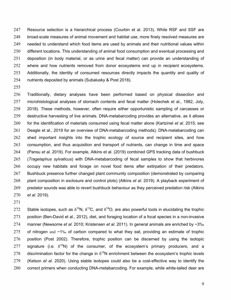
606 Figure 1: Meta-ecosystem model characterizing the trophic structure and dynamics of nutrients 607 (N), plants (P), herbivores (H) and carnivores (C) within and between four local ecosystems. In 608 the model carnivore abundance changes as a function of assimilated intake of 609 herbivore biomass within ecosystem 𝑖 (1- 𝛾C)WC(𝐻𝑖, C𝑖), where 𝛾C is the degree of inefficiency in 610

assimilation, loss due to natural mortality at rate LC(𝐶𝑖), and gain due to 611

migration from another local ecosystem dC ∑(𝑗=1) cijCj, where dC is the movement rate of a 612

carnivore and cij is the spatial connectivity between two local ecosystems (where high values 613 reflect high connectivity and hence high ease of flow). Herbivore abundance changes as a 614 function of assimilated intake of plant biomass (1- 𝛾𝐻 )WH(𝑃𝑖, H𝑖), loss due to natural mortality at 615

rate LH(𝐻𝑖), loss due to predation at rate WC(𝐻𝑖, C𝑖 ) and gain due to migration from another local 616

ecosystem dH ∑(𝑗=1)cijHj. Plant biomass changes as a function of nutrient uptake at rate 𝑈(𝑁𝑖, 𝑃𝑖), 617

loss due to senescence at rate M(𝑃𝑖) and herbivory at rate WH(𝑃𝑖, H𝑖). Finally nutrient 618

abundance changes due to global inputs I from weathering of parent geological material, 619 release from riverine sediments, wind-born dust, or rain-driven and snowmelt-driven run-620 off, loss due to leaching out of the ecosystem E𝑁𝑖 and plant uptake at rate 𝑈(𝑁𝑖, 𝑃𝑖), and 621

!"#

!$=I– E*+ – U(*+,/+)+2M(/+)

+45 LH(5+)+48 LC(8+)+:5W(/+,H+)+:8W(5+,C+)

+dH∑>?@A

cij :5W(/E, HE)+ dC ∑>?@A

cij :8W(5E, CE)

!F#

!$=G(*+,/+)- M(/+)- W(/+,HE)

!I#

!$=(1- :5 )WH(/+,H+) - LH(5+)+dH∑>?@

AcijHj - WC(5+,C+)

!K#

!$=(1- :C)WC(5+,C+) - LC(8+)+dC∑>?@

AcijCj

Ecosystem model component

Trophic interactionswithin and between local ecosystems

Nutrient translocation and depositiondue to within-ecosystem carcass and nutrient deposition and between ecosystem nutrient deposition

C

H

P

N

C

H

P

N

C

H

P

N

C

H

P

N

1 2

3 4

Spatial measurements needed (sections)

(i) The spatial extent and spatial grain size of animal movement(ii) Habitat structure shaping where animals move

(iii) Available and selected resources(iv) Movement rates directional spatial flow of animals and nutrients(v) Amount of animal carcass and nutrients deposited spatially

21

additions due to recycling of plant material 𝜖M(𝑃𝑖), herbivore and carnivore carcasses at 622

rates 𝜒𝐻LH(𝐻𝑖) + 𝜒𝐶LC(𝐶𝑖), and release of unassimilated consumption by herbivores an 623

carnivores (e.g. egesta) at rates 𝛾𝐻W(𝑃𝑖, H𝑖) + 𝛾𝐶W(𝐻𝑖, C𝑖). Local ecosystem nutrient budgets 624

are also subsidized by unassimilated nutrient release as herbivores and carnivores migrate 625 among local ecosystems dH ∑_(𝑗=1) cij 𝛾𝐻W𝑃𝑗, H𝑗) + dC ∑_(𝑗=1) cij 𝛾𝐶W(𝐻𝑗, C𝑗). These components 626

describing nutrient dynamics can ultimately be grouped according to two broad spatial 627 processes: spatial trophic interactions and spatial nutrient translocation and deposition. These 628 spatial processes can be further decomposed into five subprocesses that require different 629 methodologies to measure. A coherent picture of spatial nutrient dynamics can be developed 630 when data from the five subprocess measurements are combined into a dynamic map that 631 portrays spatial animal movement and nutrient flow in relation to the biophysical features within 632 and between local ecosystems across a landscape. Model and illustration adapted from 633 Marleau et al. (2014). 634 635

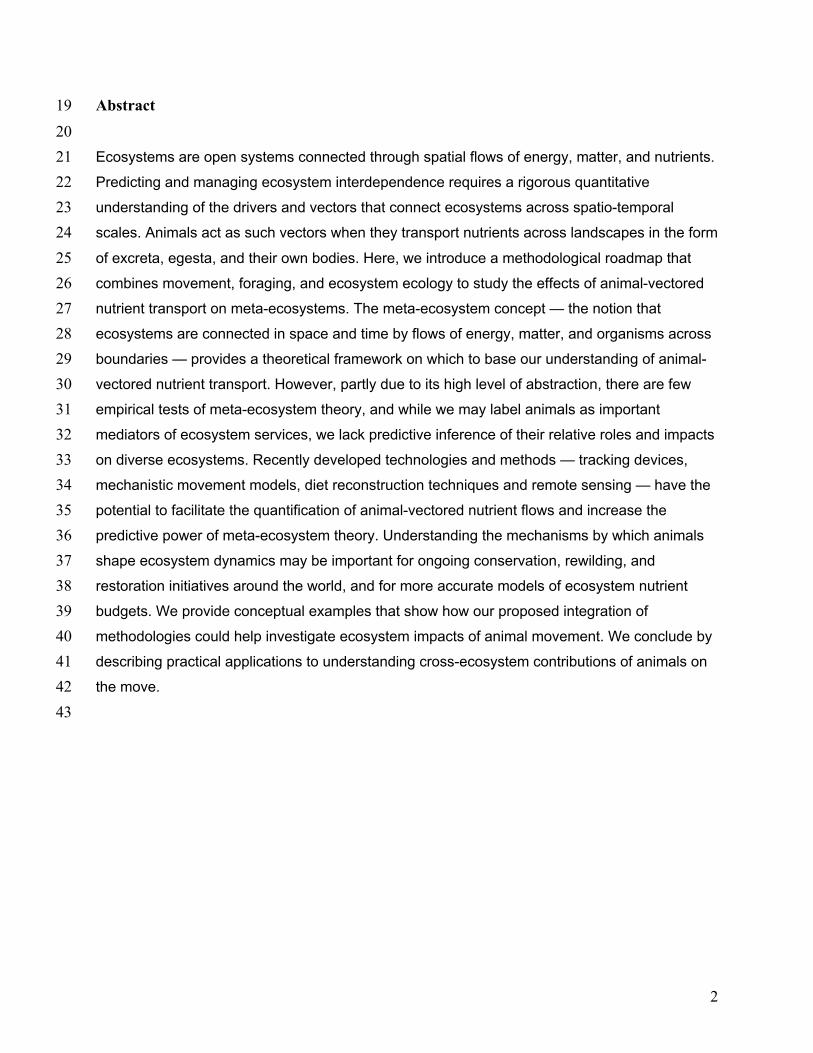
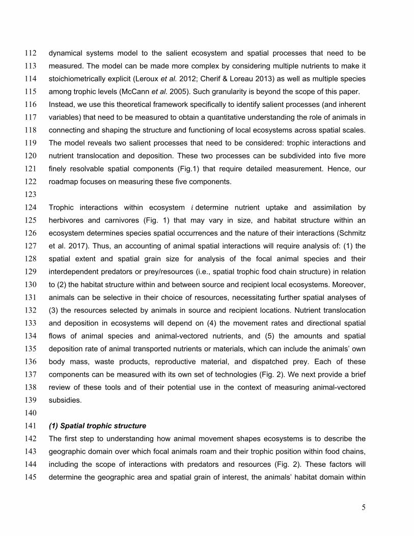
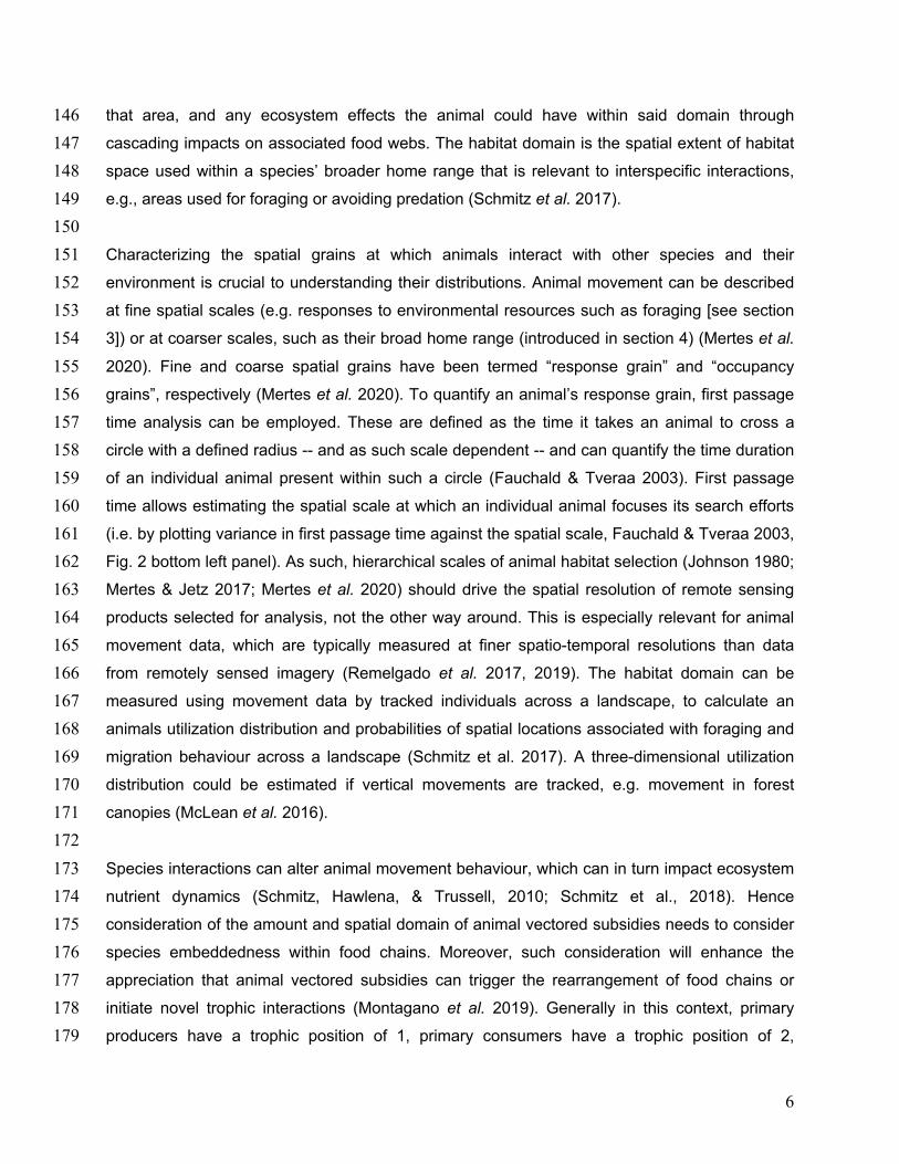
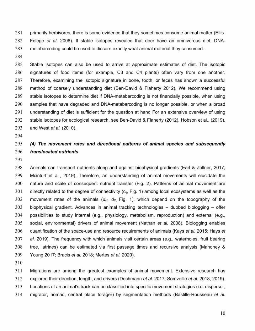
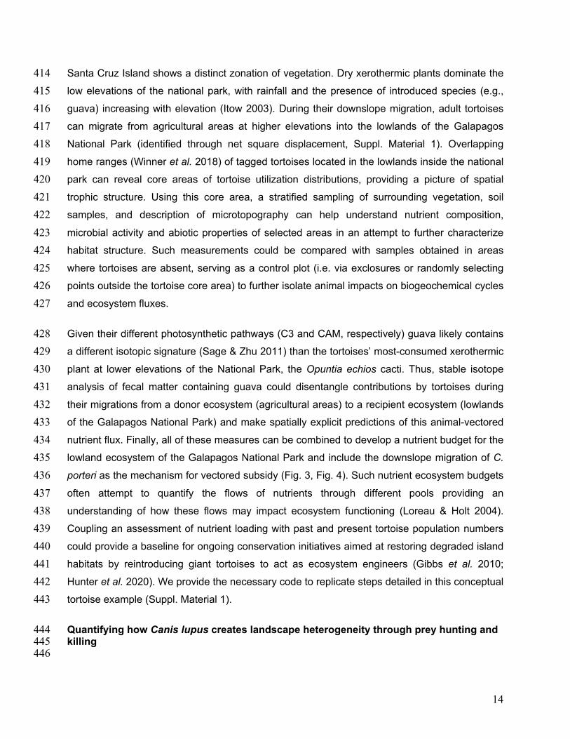
636 Figure 2: Conceptual demonstration of integrating different disciplines (sections 1,-4) for 637 quantifying animal vectorized subsidies across a landscape (section 5). (i) The habitat domain 638 helps understand the trophic position. In our hypothetical example, a roe deer (Capreolus 639 capreolus) travels across yellow patches containing agricultural areas and a green patch with 640 forested area. A first passage time analysis would reveal the scale of roe deer selection to be 641

ForestAgriculture

Water

Lidar

(i) Habitat domain

Stable Isotope Behavioral classification

Forage Travel

Home range analysis

Latit

ude

Longitude

100m

100m Varia

nce

of lo

g (F

PT)

Distance

1000m

Landcover

First PassageTime

(ii) Habitat structure (iv) Animal movement

Nutrient mapping

(v) Quantify animalvectorized subsidies

Trophic position

(iii) Resource selection

δ15N δ13C

δ18O

DNA-metabarcoding

Freq

uenc

y

SpeciesA B C

Nutrient budget model

22

strongest at approximately 100m. With this knowledge we can proceed on estimating the trophic 642 positions and interactions at that scale, choosing subsequent remote sensing products at the 643 same spatial scale. If we were to select a scale of 1000m – where extensive remove sensing 644 products are available (Table 1), we would see a weaker response of animals selecting their 645 environment. (ii) The habitat structure of our study region can be identified through remotely 646 sensed products, such as landcover maps. In this example, agriculture and water would be 647 convex ecosystems and likely receive abiotic inputs from forest leaves (concave ecosystem) 648 due to runoff. Convex and concave can be defined with elevation products or with Lidar to 649 obtain a 3D matrix of the environment across which animals navigate (i.e. against elevation 650 gradients during animal upslope movement). Lidar imagery was created using the rLidar and 651 rGedi packages. Habitat and environmental information (ii) can then be used as response 652 variables to understand how animals select and avoid resources and associated habitat 653 structures, using resource selection. Such resource use map is displayed in (iii) with green 654 colors indicating hotspots of habitat selection by our animal. Further, DNA-metabarcoding (iii) of 655 animal fecal matter in the study region can reveal the trophic position and the resources 656 consumed and deposited at great taxonomic detail. Understanding the stoichiometry of 657 resources consumed through stable isotopes (iii) provides insights into the composition and type 658 of nutrients that are moved by animals. (iv) Detailed information of roe deer movement obtained 659 through GPS collars reveals detailed space use of individuals (i.e. their home range) which can 660 be overlaid with the habitat structure of the landscape. Behavioural change point analysis (iv) 661 based on movement data could classify animal behaviour into foraging and travel. Coupling 662 behavioural classification and animal movement with faecal sampling for DNA-metabarcoding 663 and stable isotope can reveal sources (foraging locations) and sinks (excretion locations) of roe 664 deer-vectorized subsidies. (v) Integrating the different methodologies described, allows 665 quantifyng animal-vectorized subsidies through spatial modelling such as Stoichiometric 666 Distribution Models (section v; Leroux et al. 2017). Importantly, coupling such models with 667 abiotic nutrient deposition rates (e. g. leaching), allows us to contextualize the magnitude and 668 direction of biotic nutrient deposition rates. We could thus begin including animal vectorized 669 subsidies into ecosystem nutrient budget models (in our hypothetical case the roe deer brings 670 nutrients from the agricultural matrix into the forest ecosystem). Integrating these steps (i-v) 671 allows us to paint a picture of the landscape in which the ecological consequences of moving 672 animals are incorporated into cross-ecosystem models. Silhouettes were obtained from the 673 PhyloPic website (phylopic.org). 674 675

23

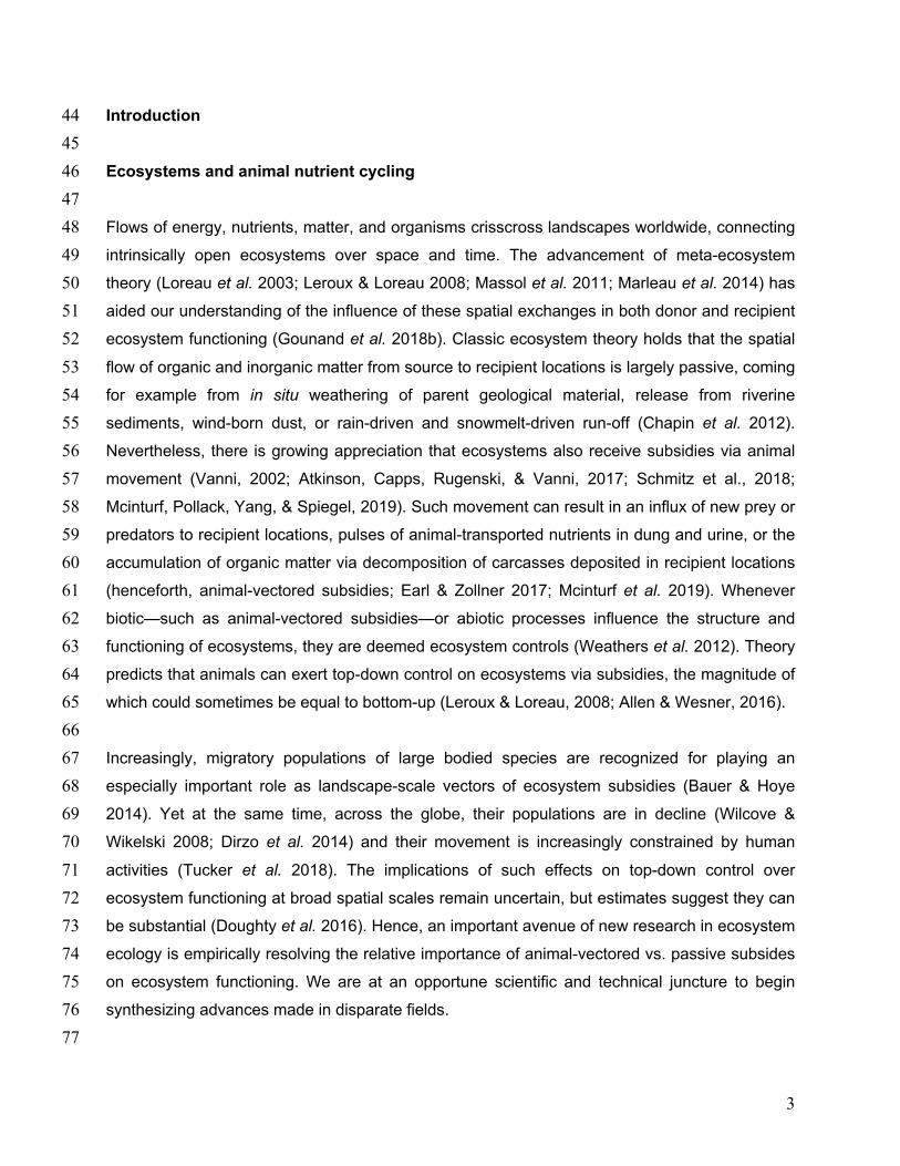
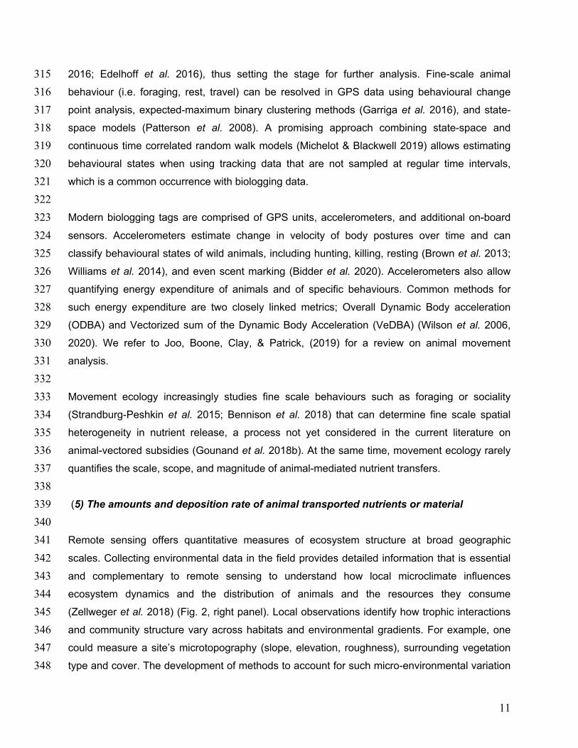
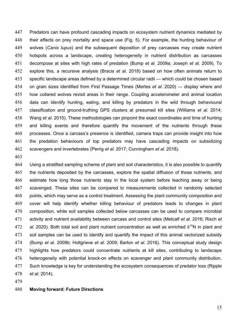
676 Figure 3: Integration of diverse disciplines and methodologies to characterize animal-vectored 677 subsidies; in this case nitrogen recycling and translocation by Galapagos tortoises (Chelonoidis 678 porteri) in time and space. (a) Movement determines the timing and direction of animal arrival 679 and departure of ecosystems. (b) Ecosystem nutrient budgets incorporate inputs from outside 680 ecosystem boundaries, such as animal-vectorized subsidies. (c) Careful sample design helps 681 elucidating drivers and predict consequences of nutrient transport by animals. Coupling large 682 extent (remote sensing, drones) with local field measurements (manual, drones) and animal 683 population estimates, allows (d) quantifying magnitude and flow of animal-vectorized subsidies 684 in a spatially explicit manner and estimate what proportion of total nutrients are being mobilized 685 by animals on the move. Tortoise silhouettes were obtained from the PhyloPic website 686 (phylopic.org). 687 688

Movement Ecosystem Prediction

Ntot = Nrecip + Nsource

Ntotal = Nsource

Migration(Translocation)

Sample design

Highlandrange(Source)

Lowlandrange(Recipie0nt)

C:N:P ratioHigh

Low

Latrine site

Drone

Manualobservations

Nutrient recycling

Nutrient translocation(Highland - Lowland)

Downslope migration(R)est, (F)orage, (T)ravel

Behavioral segmentation

Home range

Rest

TravelForage

24

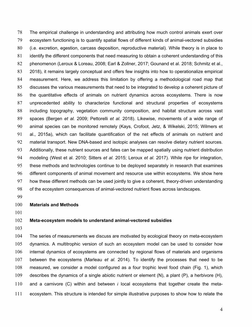
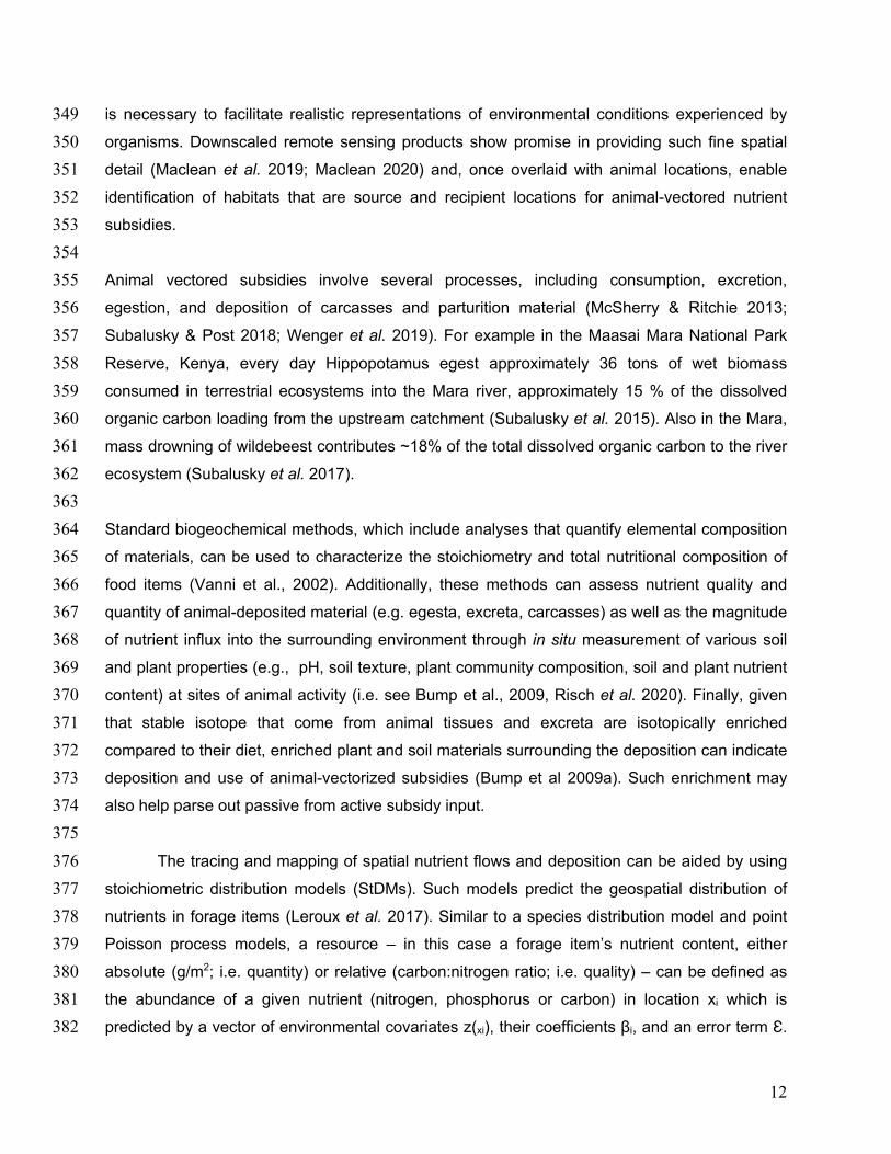
689 Figure 4: Conceptual example of studying nutrient transport of giant tortoises (Chelonidis 690 porteri) in Santa Cruz Island. Integrating known movement patterns and foraging behaviour of 691 this species with the distribution and nutritional composition of food items, it is possible to 692 design an experiment to estimate the influence of tortoises transporting nutrients to the 693 Galapagos National Park boundaries during their downslope migration. Silhouettes were 694 obtained from the PhyloPic website (phylopic.org). 695 696

(section i, ii, iv)

Galapagos tortoise (Chelonoidis porteri)

Migrating tortoises ”surf the green wave”

Julian day

Elev

atio

n

LongLa

t

A) Animal movement

Psidium guajava preferred food itemTree distribution

Elev

atio

n

Endmember

δN15

δC13

B) Foraging ecology

D) Spatially explicit animal vectored subsidiesC) Biogeochemistry

Map tortoise hotspots

Long

Lat

Tortoise Control

Vegetation plotsSoil samplesExclosure plotsDung decompositionFeces nutrient contentMicrotopography

Measure1 tortoise

Present population

Past population

Long

Lat

C, N, P

C, N, P

C, N, P

(section ii, iii)

(section ii, v) (section v)

25

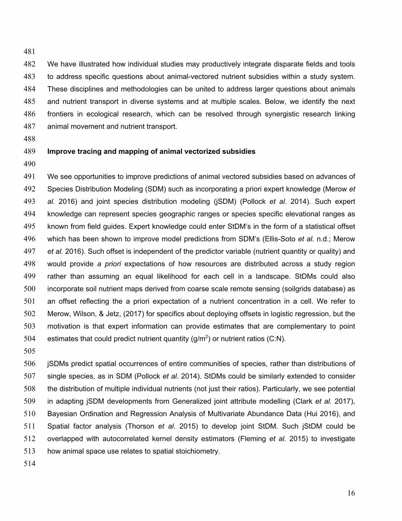
697 Figure 5: Conceptual example to identify killing sites of Wolfes (Canis lupus) with biologging 698 technologies and quantify how predators drive landscape heterogeneity. Identifying kill sites 699 allows studyng how carcass presence affects local biogeochemistry and community 700 composition when compared to control locations. Silhouettes were obtained from the PhyloPic 701 website (phylopic.org). 702 703 Table 1: Collection of applicable remote sensing products for animal mediated subsidies. We 704 elucidate the spatio-temporal resolution and grain size of these products. 705 706 Appendix – Supplementary Material 707 708 Supplementary Material 1: Necessary code to perform movement ecology and remote 709 sensing analysis of the Galapagos tortoise example 710 711 References 712 713 Abbas, F., Merlet, J., Morellet, N., Verheyden, H., Hewison, A.J.M., Cargnelutti, B., et al. (2012). 714

Roe deer may markedly alter forest nitrogen and phosphorus budgets across Europe, 1–8. 715 Allan, B.M., Nimmo, D.G., Ierodiaconou, D., VanDerWal, J., Koh, L.P. & Ritchie, E.G. (2018). 716

Futurecasting ecological research: the rise of technoecology. Ecosphere. 717

Wolf (Canis lupus)

D) Spatially explicit animal vectored subsidies

Time (s)

Walk Hunt Forage

Acce

lera

tion

(g) Walk

A) Animal behavior and movement

Identify hunting behavior & kill site

C) Biogeochemistry

B) Community ecology

Carcasses enhance invertebrate and scavenger diversityChange in plant communityControl

t(0) t(1) t(2)

Control

Stratified sampling

Vegetation plotsSoil samplesMicrotopographyMicrobial activity

Impact of prey killing on landscape heterogeneity

Compare predator impact withgame hunting carcass deposition

Study trophic cascade causedby absence of predators

Lat

Kill site

Long

Control

(section i, iv)

(section ii, v)

(section i, ii)

(section v)

26

Allen, C.D. & Wesner, S.J. (2016). Synthesis: comparing effects of resource and consumer 718 fluxes into recipient food webs using meta- analysis. Ecology, 97, 594–604. 719

Amatulli, G., Domisch, S., Tuanmu, M.-N., Parmentier, B., Ranipeta, A., Malczyk, J., et al. 720 (2018). A suite of global, cross-scale topographic variables for environmental and 721 biodiversity modeling. Sci. Data, 5, 180040. 722

de Araujo Barbosa, C.C., Atkinson, P.M. & Dearing, J.A. (2015). Remote sensing of ecosystem 723 services: A systematic review. Ecol. Indic., 52, 430–443. 724

Atkins, J.L., Long, R.A., Pansu, J., Daskin, J.H., Potter, A.B., Stalmans, M.E., et al. (2019). 725 Cascading impacts of large-carnivore extirpation in an African ecosystem. Science (80-. )., 726 364, 173–177. 727

Atkinson, C.L., Capps, K.A., Rugenski, A.T. & Vanni, M.J. (2017). Consumer-driven nutrient 728 dynamics in freshwater ecosystems : from individuals to ecosystems. Biol. Rev., 92, 2003–729 2023. 730

Avgar, T., Potts, J.R., Lewis, M.A. & Boyce, M.S. (2016). Integrated step selection analysis: 731 bridging the gap between resource selection and animal movement. Methods Ecol. Evol., 732 7, 619–630. 733

Bampoh, D., Earl, J.E. & Zollner, P.A. (2019). Examining the relative influence of animal 734 movement patterns and mortality models on the distribution of animal transported 735 subsidies. Ecol. Modell., 412, 108824. 736

Barton, P.S., McIntyre, S., Evans, M.J., Bump, J.K., Cunningham, S.A. & Manning, A.D. (2016). 737 Substantial long-term effects of carcass addition on soil and plants in a grassy eucalypt 738 woodland. Ecosphere, 7, e01537. 739

Bastille-Rousseau, G., Gibbs, J.P., Campbell, K., Yackulic, C.B. & Blake, S. (2017). Ecosystem 740 implications of conserving endemic versus eradicating introduced large herbivores in the 741 Galapagos Archipelago. Biol. Conserv., 209, 1–10. 742

Bastille-Rousseau, G., Potts, J.R., Yackulic, C.B., Frair, J.L., Ellington, E.H. & Blake, S. (2016). 743 Flexible characterization of animal movement pattern using net squared displacement and 744 a latent state model. Mov. Ecol., 4, 15. 745

Bastille-Rousseau, G., Yackulic, C., Gibbs, J., Frair, J., Cabrera, F. & Blake, S. (2019). 746 Migration triggers in a large herbivore: Galapagos giant tortoises navigating resource 747 gradients on volcanoes. Ecology, 100, 1–11. 748

Bauer, S. & Hoye, B.J. (2014). Migratory animals couple biodiversity and ecosystem functioning 749 worldwide. Science (80-. )., 344. 750

Bello, C., Galetti, M., Pizo, M.A., Magnago, L.F.S., Rocha, M.F., Lima, R.A.F., et al. (2015). 751

27

Defaunation affects carbon storage in tropical forests. Sci. Adv., 1, e1501105. 752 Ben-David, M. & Flaherty, E.A. (2012). Stable isotopes in mammalian research: a beginner’s 753

guide. J. Mammal., 93, 312–328. 754 Bennison, A., Bearhop, S., Bodey, T.W., Votier, S.C., Grecian, W.J., Wakefield, E.D., et al. 755

(2018). Search and foraging behaviors from movement data: A comparison of methods. 756 Ecol. Evol., 8, 13–24. 757

Bergen, K.M., Goetz, S.J., Dubayah, R.O., Henebry, G.M., Hunsaker, C.T., Imhoff, M.L., et al. 758 (2009). Remote sensing of vegetation 3-D structure for biodiversity and habitat: Review 759 and implications for lidar and radar spaceborne missions. J. Geophys. Res. 760 Biogeosciences, 114, G00E06. 761

Berzaghi, F., Verbeeck, H., Nielsen, M.R., Doughty, C.E., Bretagnolle, F., Marchetti, M., et al. 762 (2018). Assessing the role of megafauna in tropical forest ecosystems and biogeochemical 763 cycles - the potential of vegetation models. Ecography (Cop.)., 1934–1954. 764

Bidder, O.R., di Virgilio, A., Hunter, J.S., McInturff, A., Gaynor, K.M., Smith, A.M., et al. (2020). 765 Monitoring canid scent marking in space and time using a biologging and machine learning 766 approach. Sci. Rep., 10, 588. 767

Blake, S., Guézou, A., Deem, S.L., Yackulic, C.B. & Cabrera, F. (2015). The Dominance of 768 Introduced Plant Species in the Diets of Migratory Galapagos Tortoises Increases with 769 Elevation on a Human-Occupied Island. Biotropica, 47, 246–258. 770

Blake, S., Wikelski, M., Cabrera, F., Guezou, A., Silva, M., Sadeghayobi, E., et al. (2012). Seed 771 dispersal by Galapagos tortoises. J. Biogeogr., 39, 1961–1972. 772

Boyce, M.S., Vernier, P.R., Nielsen, S.E. & Schmiegelow, F.K.A. (2002). Evaluating resource 773 selection functions. Ecol. Modell., 281–300. 774

Bracis, C., Bildstein, K.L. & Mueller, T. (2018). Revisitation analysis uncovers spatio-temporal 775 patterns in animal movement data. Ecography (Cop.)., 41, 1801–1811. 776

Brown, D.D., Kays, R., Wikelski, M., Wilson, R. & Klimley, A.P. (2013). Observing the 777 unwatchable through acceleration logging of animal behavior. Anim. Biotelemetry, 1, 1–20. 778

Bump, J.K., Webster, C.R., Vucetich, J.A., Peterson, R.O., Shields, J.M. & Powers, M.D. 779 (2009a). Ungulate Carcasses Perforate Ecological Filters and Create Biogeochemical 780 Hotspots in Forest Herbaceous Layers Allowing Trees a Competitive Advantage. 781 Ecosystems, 12, 996–1007. 782

Bump, K.J., Rolf, O.P. & Vucetich, A.J. (2009b). Wolves modulate soil nutrient heterogeneity 783 and foliar nitrogen by configuring the distribution of ungulate carcasses. Ecology, 90, 784 3159–3167. 785

28

Chapin, F.S., Matson, P.A. & Vitousek, P.M. (2012). Principles of terrestrial ecosystem ecology. 786 Princ. Terr. Ecosyst. Ecol. Springer. 787

Cherif, M. & Loreau, M. (2013). Plant-herbivore-decomposer stoichiometric mismatches and 788 nutrient cycling in ecosystems. Proc. R. Soc. B Biol. Sci., 280, 20122453. 789

Clark, B.L., Bevanda, M., Aspillaga, E. & Jørgensen, N.H. (2016). Bridging disciplines with 790 training in remote sensing for animal movement: an attendee perspective. Remote Sens. 791 Ecol. Conserv., 3, 30–37. 792

Clark, J.S., Nemergut, D., Seyednasrollah, B., Turner, P.J. & Zhang, S. (2017). Generalized 793 joint attribute modeling for biodiversity analysis: median-zero, multivariate, multifarious 794 data. Ecol. Monogr., 87, 34–56. 795

Cunningham, C.X., Johnson, C.N., Barmuta, L.A., Hollings, T., Woehler, E.J. & Jones, M.E. 796 (2018). Top carnivore decline has cascading effects on scavengers and carrion 797 persistence. Proc. R. Soc. B Biol. Sci., 285, 20181582. 798

Davies, A.B. & Asner, G.P. (2019). Elephants limit aboveground carbon gains in African 799 savannas. Glob. Chang. Biol., 25, 1368–1382. 800

Deagle, B.E., Thomas, A.C., McInnes, J.C., Clarke, L.J., Vesterinen, E.J., Clare, E.L., et al. 801 (2019). Counting with DNA in metabarcoding studies: How should we convert sequence 802 reads to dietary data? Mol. Ecol., 28, 391–406. 803

Dechmann, D.K.N., Wikelski, M., Ellis-Soto, D., Safi, K. & Teague O’Mara, M. (2017). 804 Determinants of spring migration departure decision in a bat. Biol. Lett. 805

Dirzo, R., Young, H.S., Galetti, M., Ceballos, G., Isaac, N.J.B. & Collen, B. (2014). Defaunation 806 in the Anthropocene. Science (80-. ). 807

Doughty, C.E. (2017). Herbivores increase the global availability of nutrients over millions of 808 years. Nat. Ecol. Evol., 1, 1820–1827. 809

Doughty, C.E., Roman, J., Faurby, S., Wolf, A., Haque, A., Bakker, E.S., et al. (2016). Global 810 nutrient transport in a world of giants. Proc. Natl. Acad. Sci. U. S. A., 113, 868–73. 811

Durán, S.M., Martin, R.E., Díaz, S., Maitner, B.S., Malhi, Y., Salinas, N., et al. (2019). Informing 812 trait-based ecology by assessing remotely sensed functional diversity across a broad 813 tropical temperature gradient. Sci. Adv., 5, eaaw8114. 814

Earl, J.E. & Zollner, P.A. (2017). Advancing research on animal-transported subsidies by 815 integrating animal movement and ecosystem modelling. J. Anim. Ecol., 86, 987–997. 816

Edelhoff, H., Signer, J. & Balkenhol, N. (2016). Path segmentation for beginners: An overview of 817 current methods for detecting changes in animal movement patterns. Mov. Ecol., 4. 818

Ellis-Felege, S.N., Burnam, J.S., Palmer, W.E., Sisson, D.C., Wellendorf, S.D., Thornton, R.P., 819

29

et al. (2008). Cameras Identify White-tailed Deer Depredating Northern Bobwhite Nests. 820 Southeast. Nat., 7, 562–564. 821

Ellis-Soto, D., Blake, S., Soultan, A., Guézou, A., Cabrera, F. & Lötters, S. (2017). Plant species 822 dispersed by Galapagos tortoises surf the wave of habitat suitability under anthropogenic 823 climate change. PLoS One, 12, e0181333. 824

Ellis-Soto, D., Merow, C., Amatulli, G., Parra, J.L. & Jetz, W. (n.d.). Continental-scale 1km 825 hummingbird diversity derived from fusing point records with lateral and elevational expert 826 information. Ecography (Cop.)., in review. 827

Ellis Soto, D. (2020). Giant tortoises connecting terrestrial and freshwater ecosystems in Santa 828 Cruz Island. In: Galapagos Giant Tortoises (eds. Gibbs, J.P., Cayot, L.J. & Tapia, W.). 829 Elsevier, Amsterdam, p. 286. 830

Falcon Wilfredo & Hansen, D.M. (2018). Island rewilding with giant tortoises in an era of climate 831 change. 832

Fauchald, P. & Tveraa, T. (2003). USING FIRST-PASSAGE TIME IN THE ANALYSIS OF 833 AREA-RESTRICTED SEARCH AND HABITAT SELECTION. Ecology, 84, 282–288. 834

Fleming, C.H., Fagan, W.F., Mueller, T., Olson, K.A., Leimgruber, P. & Calabrese, J.M. (2015). 835 Rigorous home range estimation with movement data: a new autocorrelated kernel density 836 estimator. Ecology, 96, 1182–1188. 837

Fortin, D., Beyer, H.L., Boyce, M.S., Smith, D.W., Duchesne, T. & Mao, J.S. (2005). Wolves 838 influence elk movements: Behavior shapes a trophic cascade in Yellowstone National 839 Park. Ecology. 840

Garriga, J., Palmer, J.R.B., Oltra, A. & Bartumeus, F. (2016). Expectation-Maximization Binary 841 Clustering for Behavioural Annotation. PLoS One, 11, e0151984. 842

Gibbs, J.P., Sterling, E.J. & Zabala, F.J. (2010). Giant tortoises as ecological engineers: A long-843 term quasi-experiment in the Gal??pagos Islands. Biotropica, 42, 208–214. 844

Gounand, I., Harvey, E., Little, C.J. & Altermatt, F. (2018a). Meta-Ecosystems 2.0: Rooting the 845 Theory into the Field. Trends Ecol. Evol., 33, 36–46. 846

Gounand, I., Little, C.J., Harvey, E. & Altermatt, F. (2018b). Cross-ecosystem carbon flows 847 connecting ecosystems worldwide. Nat. Commun., 9, 4825. 848

Hancock, S., Hofton, M., Sun, X., Tang, H., Kellner, J.R., Armston, J., et al. (2019). The GEDI 849 simulator: A large-footprint waveform lidar simulator for calibration and validation of 850 spaceborne missions. Earth Sp. Sci., 294–310. 851

Hays, G.C., Bailey, H., Bograd, S.J., Bowen, W.D., Campagna, C., Carmichael, R.H., et al. 852 (2019). Translating Marine Animal Tracking Data into Conservation Policy and 853

30

Management. Trends Ecol. Evol., xx, 1–15. 854 Hirt, M.R., Grimm, V., Li, Y., Rall, B.C., Rosenbaum, B. & Brose, U. (2018). Bridging Scales: 855

Allometric Random Walks Link Movement and Biodiversity Research. Trends Ecol. Evol., 856 33, 701–712. 857

Hobson, K.A., Wassenaar, L.I., Bowen, G.J., Courtiol, A., Trueman, C.N., Voigt, C.C., et al. 858 (2019). Chapter 10 - Outlook for Using Stable Isotopes in Animal Migration Studies. In: 859 Tracking Animal Migration with Stable Isotopes (Second Edition) (eds. Hobson, K.A. & 860 Wassenaar, L.I.). Academic Press, pp. 237–244. 861

Holtgrieve, G.W., Schindler, D.E. & Jewett, P.K. (2009). Large predators and biogeochemical 862 hotspots: Brown bear (Ursus arctos) predation on salmon alters nitrogen cycling in riparian 863 soils. Ecol. Res. 864

Hui, F.K.C. (2016). boral – Bayesian Ordination and Regression Analysis of Multivariate 865 Abundance Data in r. Methods Ecol. Evol., 7, 744–750. 866

Hunter, E.A., Gibbs, J.P., Cayot, L.J., Tapia, W., Quinzin, M.C., Miller, J.M., et al. (2020). 867 Seeking compromise across competing goals in conservation translocations: The case of 868 the ‘extinct’ Floreana Island Galapagos giant tortoise. J. Appl. Ecol., 57, 136–148. 869

Itow, S. (2003). Zonation Pattern, Succession Process and Invasion by Aliens in Species-poor 870 Insular Vegetation of the Galápagos Islands. Glob. Environ. Res., 7, 39–58. 871

Jetz, W., Cavender-Bares, J., Pavlick, R., Schimel, D., Davis, F.W., Asner, G.P., et al. (2016). 872 Monitoring plant functional diversity from space. Nat. Plants, 2, 16024. 873

Johnson, D.H. (1980). The comparision of usage and availability measurements for evaluating 874 resource preference. Ecology, 61. 875

Joo, R., Boone, M.E., Clay, T.A. & Patrick, S.C. (2019). Navigating through the R packages for 876 movement, 1–29. 877

Joseph, K.B., Rolf, O.P. & John, A.V. (2009). Wolves modulate soil nutrient heterogeneity and 878 foliar nitrogen by configuring the distribution of ungulate carcasses. Ecology, 90, 3159–879 3167. 880

Kartzinel, T.R., Chen, P.A., Coverdale, T.C., Erickson, D.L., Kress, W.J., Kuzmina, M.L., et al. 881 (2015). DNA metabarcoding illuminates dietary niche partitioning by African large 882 herbivores. Proc. Natl. Acad. Sci., 112, 8019–8024. 883

Kays, R., Crofoot, M.C., Jetz, W. & Wikelski, M. (2015). Terrestrial animal tracking as an eye on 884 life and planet. Science (80-. )., 348, aaa2478. 885

Kelson, S.J., Power, M.E., Finlay, J.C. & Carlson, S.M. (2020). Partial migration alters 886 population ecology and food chain length: evidence from a salmonid fish. Ecosphere, 11, 887

31

e03044. 888 Kie, J.G., Matthiopoulos, J., Fieberg, J., Powell, R.A., Cagnacci, F., Mitchell, M.S., et al. (2010). 889

The home-range concept: are traditional estimators still relevant with modern telemetry 890 technology? Philos. Trans. R. Soc. B Biol. Sci., 365, 2221–2231. 891

Kitchell, J.F., Schindler, D.E., Herwig, B.R., Post, D.M., Olson, M.H. & Oldham, M. (1999). 892 Nutrient cycling at the landscape scale: The role of diel foraging migrations by geese at the 893 Bosque del Apache National Wildlife Refuge, New Mexico. Limnol. Oceanogr. 894

Kleyheeg, E., Fiedler, W., Safi, K., Waldenström, J., Wikelski, M. & van Toor, M.L. (2019). A 895 Comprehensive Model for the Quantitative Estimation of Seed Dispersal by Migratory 896 Mallards. Front. Ecol. Evol., 7, 1–14. 897

Knyazikhin, Y., Schull, M.A., Stenberg, P., Mõttus, M., Rautiainen, M., Yang, Y., et al. (2013). 898 Hyperspectral remote sensing of foliar nitrogen content. Proc. Natl. Acad. Sci., 110, E185--899 E192. 900

Kristensen, D.K., Kristensen, E., Forchhammer, M.C., Michelsen, A. & Schmidt, N.M. (2011). 901 Arctic herbivore diet can be inferred from stable carbon and nitrogen isotopes in C3 plants, 902 faeces, and wool. Can. J. Zool., 89, 892–899. 903

Laso, F.J., Ben, L., Rivas-torres, G., Sampedro, C. & Arce-nazario, J. (2019). Land Cover 904 Classification of Complex Agroecosystems in the Non-Protected Highlands of the 905 Galapagos Islands. 906

Leroux, S.J., Hawlena, D. & Schmitz, O.J. (2012). Predation risk, stoichiometric plasticity and 907 ecosystem elemental cycling. Proc. R. Soc. B Biol. Sci., 279, 4183–4191. 908

Leroux, S.J. & Loreau, M. (2008). Subsidy hypothesis and strength of trophic cascades across 909 ecosystems. Ecol. Lett., 11, 1147–1156. 910

Leroux, S.J. & Loreau, M. (2012). Dynamics of Reciprocal Pulsed Subsidies in Local and Meta-911 Ecosystems. Ecosystems, 15, 48–59. 912

Leroux, S.J., Wal, E. Vander, Wiersma, Y.F., Charron, L., Ebel, J.D., Ellis, N.M., et al. (2017). 913 Stoichiometric distribution models: ecological stoichiometry at the landscape extent. Ecol. 914 Lett., 20, 1495–1506. 915

Lindeman, R.L. (1942). The Trophic-Dynamic Aspect of Ecology. Ecology, 23, 399–417. 916 Loreau, M. & Holt, R.D. (2004). Spatial Flows and the Regulation of Ecosystems. Am. Nat., 163, 917

606–615. 918 Loreau, M., Mouquet, N. & Holt, R.D. (2003). IDEAS AND Meta-ecosystems : a theoretical 919

framework for a spatial ecosystem ecology, 673–679. 920 Lundgren, E.J., Ramp, D., Ripple, W.J. & Wallach, A.D. (2018). Introduced megafauna are 921

32

rewilding the Anthropocene. Ecography (Cop.)., 41, 857–866. 922 Maclean, I.M.D. (2020). Predicting future climate at high spatial and temporal resolution. Glob. 923

Chang. Biol., 26, 1003–1011. 924 Maclean, I.M.D., Mosedale, J.R. & Bennie, J.J. (2019). Microclima: An r package for modelling 925

meso- and microclimate. Methods Ecol. Evol., 10. 926 Magioli, M., Moreira, M.Z., Fonseca, R.C.B., Ribeiro, M.C., Rodrigues, M.G. & Ferraz, K.M.P.M. 927

de B. (2019). Human-modified landscapes alter mammal resource and habitat use and 928 trophic structure. Proc. Natl. Acad. Sci., 116, 18466–18472. 929

Mahoney, P.J. & Young, J.K. (2017). Uncovering behavioural states from animal activity and 930 site fidelity patterns. Methods Ecol. Evol., 8, 174–183. 931

Marleau, J.N., Guichard, F. & Loreau, M. (2014). Meta-ecosystem dynamics and functioning on 932 finite spatial networks. Proc. R. Soc. B Biol. Sci. 933

Massol, F., Gravel, D., Mouquet, N., Cadotte, M.W., Fukami, T. & Leibold, M.A. (2011). Linking 934 community and ecosystem dynamics through spatial ecology. Ecol. Lett., 14, 313–323. 935

McCann, K.S., Rasmussen, J.B. & Umbanhowar, J. (2005). The dynamics of spatially coupled 936 food webs. Ecol. Lett., 8, 513–523. 937

Mcinturf, A.G., Pollack, L., Yang, L.H. & Spiegel, O. (2019). Vectors with autonomy : what 938 distinguishes animal-mediated nutrient transport from abiotic vectors ? 939

McLean, K.A., Trainor, A.M., Asner, G.P., Crofoot, M.C., Hopkins, M.E., Campbell, C.J., et al. 940 (2016). Movement patterns of three arboreal primates in a Neotropical moist forest 941 explained by LiDAR-estimated canopy structure. Landsc. Ecol., 31, 1849–1862. 942

McSherry, M.E. & Ritchie, M.E. (2013). Effects of grazing on grassland soil carbon: a global 943 review. Glob. Chang. Biol., 19, 1347–1357. 944

Merow, C., Allen, J.M., Aiello-Lammens, M. & Silander, J.A. (2016). Improving niche and range 945 estimates with Maxent and point process models by integrating spatially explicit 946 information. Glob. Ecol. Biogeogr., 25, 1022–1036. 947

Merow, C., Wilson, A.M. & Jetz, W. (2017). Integrating occurrence data and expert maps for 948 improved species range predictions. Glob. Ecol. Biogeogr., 26, 243–258. 949

Mertes, K., Jarzyna, M.A. & Jetz, W. (2020). Hierarchical multi-grain models improve 950 descriptions of species’ environmental associations, distribution, and abundance. Ecol. 951 Appl. 952

Mertes, K. & Jetz, W. (2017). Disentangling scale dependencies in species environmental 953 niches and distributions. Ecography (Cop.). 954

Metcalf, J.L., Xu, Z.Z., Weiss, S., Lax, S., Van Treuren, W., Hyde, E.R., et al. (2016). Microbial 955

33

community assembly and metabolic function during mammalian corpse decomposition. 956 Science (80-. ). 957

Michelot, T. & Blackwell, P.G. (2019). State-switching continuous-time correlated random walks. 958 Methods Ecol. Evol., 0, 1–13. 959

Michelot, T., Blackwell, P.G. & Matthiopoulos, J. (2019). Linking resource selection and step 960 selection models for habitat preferences in animals. Ecology, 100, e02452. 961

Montagano, L., Leroux, S.J., Giroux, M.-A. & Lecomte, N. (2019). The strength of ecological 962 subsidies across ecosystems: a latitudinal gradient of direct and indirect impacts on food 963 webs. Ecol. Lett., 22, 265–274. 964

Nathan, R., Getz, W.M., Revilla, E., Holyoak, M., Kadmon, R., Saltz, D., et al. (2008). A 965 movement ecology paradigm for unifying organismal movement research Ran. Pnas, 105, 966 19052–19059. 967

Nathan, R., Spiegel, O., Fortmann-Roe, S., Harel, R., Wikelski, M. & Getz, W.M. (2012). Using 968 tri-axial acceleration data to identify behavioral modes of free-ranging animals: general 969 concepts and tools illustrated for griffon vultures. J. Exp. Biol., 215, 986–96. 970

Newsome, S.D., Clementz, M.T. & Koch, P.L. (2010). Using stable isotope biogeochemistry to 971 study marine mammal ecology. Mar. Mammal Sci., 26, 509–572. 972

Pansu, J., Guyton, J.A., Potter, A.B., Atkins, J.L., Daskin, J.H., Wursten, B., et al. (2019). 973 Trophic ecology of large herbivores in a reassembling African ecosystem. J. Ecol., 107, 974 1355–1376. 975

Patterson, T.A., Thomas, L., Wilcox, C., Ovaskainen, O. & Matthiopoulos, J. (2008). 976 State–space models of individual animal movement. Trends Ecol. Evol., 23, 87–977 94. 978

Perrig, P.L., Donadio, E., Middleton, A.D. & Pauli, J.N. (2017). Puma predation subsidizes an 979 obligate scavenger in the high Andes. J. Appl. Ecol., 54, 846–853. 980

Pettorelli, N., Laurance, W.F., O’Brien, T.G., Wegmann, M., Nagendra, H. & Turner, W. (2014). 981 Satellite remote sensing for applied ecologists: Opportunities and challenges. J. Appl. 982 Ecol., 51, 839–848. 983

Pettorelli, N., to Bühne, H., Tulloch, A., Dubois, G., Macinnis-Ng, C., Queirós, A.M., et al. 984 (2018). Satellite remote sensing of ecosystem functions: opportunities, challenges and way 985 forward. Remote Sens. Ecol. Conserv., 4, 71–93. 986

Picardi, S., Smith, B.J., Boone, M.E., Frederick, P.C., Cecere, J.G., Rubolini, D., et al. (2019). A 987 data-driven method to locate nest sites and estimate reproductive outcome from avian 988 telemetry data. bioRxiv, 562025. 989

34

Pollock, L.J., Tingley, R., Morris, W.K., Golding, N., O’Hara, R.B., Parris, K.M., et al. (2014). 990 Understanding co-occurrence by modelling species simultaneously with a Joint Species 991 Distribution Model (JSDM). Methods Ecol. Evol., 5, 397–406. 992

Post, D.M. (2002). Using stable isotopes to estimate trophic position: Models, methods, and 993 assumptions. Ecology. 994

Remelgado, R., Leutner, B., Safi, K., Sonnenschein, R., Kuebert, C. & Wegmann, M. (2017). 995 Linking animal movement and remote sensing - mapping resource suitability from a remote 996 sensing perspective. Remote Sens. Ecol. Conserv., 1–14. 997

Remelgado, R., Wegmann, M. & Safi, K. (2019). rsmove —An r package to bridge remote 998 sensing and movement ecology . Methods Ecol. Evol. 999

Ripple, W.J., Estes, J.A., Beschta, R.L., Wilmers, C.C., Ritchie, E.G., Hebblewhite, M., et al. 1000 (2014). Status and Ecological Effects of the World’s Largest Carnivores. Science (80-. )., 1001 343, 1241484. 1002

Risch, A.C., Frossard, A., Schütz, M., Frey, B., Morris, A.W. & Bump, J.K. (2020). Effects of elk 1003 and bison carcasses on soil microbial communities and ecosystem functions in 1004 Yellowstone, USA. Funct. Ecol., 00, 1–12. 1005

Rivas-Torres, G.F., Benítez, F.L., Rueda, D., Sevilla, C. & Mena, C.F. (2018). A methodology 1006 for mapping native and invasive vegetation coverage in archipelagos: An example from the 1007 Galápagos Islands. Prog. Phys. Geogr. 1008

Sage, R.F. & Zhu, X.-G. (2011). Exploiting the engine of C(4) photosynthesis. J. Exp. Bot. 1009 Schmitz, O.J., Hawlena, D. & Trussell, G.C. (2010). Predator control of ecosystem nutrient 1010

dynamics. Ecol. Lett. 1011 Schmitz, O.J., Miller, J.R.B., Trainor, A.M. & Abrahms, B. (2017). Toward a community ecology 1012

of landscapes: predicting multiple predator–prey interactions across geographic space. 1013 Ecology, 98, 2281–2292. 1014

Schmitz, O.J., Rosenblatt, A.E. & Smylie, M. (2016). Temperature dependence of predation 1015 stress and the nutritional ecology of a generalist herbivore. Ecology, 97, 3119–3130. 1016

Schmitz, O.J., Wilmers, C.C., Leroux, S.J., Doughty, C.E., Atwood, T.B., Galetti, M., et al. 1017 (2018). Animals and the zoogeochemistry of the carbon cycle. Science (80-. )., 362, 1018 eaar3213. 1019

Schneider, F.D., Morsdorf, F., Schmid, B., Schimel, D.S., Schaepman, M.E., Petchey, O.L., et 1020 al. (2017). Mapping functional diversity from remotely sensed morphological and 1021 physiological forest traits. Nat. Commun., 8. 1022

Sitters, J., Atkinson, C.L., Guelzow, N., Kelly, P. & Sullivan, L.L. (2015). Spatial stoichiometry: 1023

35

Cross-ecosystem material flows and their impact on recipient ecosystems and organisms. 1024 Oikos, 124, 920–930. 1025

Sobral, M., Silvius, K.M., Overman, H., Oliveira, L.F.B., Raab, T.K. & Fragoso, J.M.V. (2017). 1026 Mammal diversity influences the carbon cycle through trophic interactions in the Amazon. 1027 Nat. Ecol. Evol., 1, 1670–1676. 1028

Somveille, M., Manica, A. & Rodrigues, A.S.L. (2019). Where the wild birds go: explaining the 1029 differences in migratory destinations across terrestrial bird species, 225–236. 1030

Somveille, M., Rodrigues, A.S.L. & Manica, A. (2018). Energy efficiency drives the global 1031 seasonal distribution of birds. Nat. Ecol. Evol., 2, 962–969. 1032

Strandburg-Peshkin, A., Farine, D.R., Couzin, I.D. & Crofoot, M.C. (2015). Shared decision-1033 making drives collective movement in wild baboons. Science (80-. )., 348, 1358–1361. 1034

Strandburg-Peshkin, A., Farine, D.R., Crofoot, M.C. & Couzin, I.D. (2017). Habitat and social 1035 factors shape individual decisions and emergent group structure during baboon collective 1036 movement. Elife, 6. 1037

Stuart, M.B., McGonigle, A.J.S. & Willmott, J.R. (2019). Hyperspectral Imaging in Environmental 1038 Monitoring: A Review of Recent Developments and Technological Advances in Compact 1039 Field Deployable Systems. Sensors (Basel)., 19, 3071. 1040

Subalusky, A.L., Dutton, C.L., Rosi-Marshall, E.J. & Post, D.M. (2015). The hippopotamus 1041 conveyor belt: vectors of carbon and nutrients from terrestrial grasslands to aquatic 1042 systems in sub-Saharan Africa. Freshw. Biol., 60, 512–525. 1043

Subalusky, A.L., Dutton, C.L., Rosi, E.J. & Post, D.M. (2017). Annual mass drownings of the 1044 Serengeti wildebeest migration influence nutrient cycling and storage in the Mara River. 1045 Proc. Natl. Acad. Sci., 114, 7647 LP-7652. 1046

Subalusky, A.L. & Post, D.M. (2018). Context dependency of animal resource subsidies. Biol. 1047 Rev. 1048

Thorson, J.T., Scheuerell, M.D., Shelton, A.O., See, K.E., Skaug, H.J. & Kristensen, K. (2015). 1049 Spatial factor analysis: a new tool for estimating joint species distributions and correlations 1050 in species range. Methods Ecol. Evol., 6, 627–637. 1051

van Toor, M.L., O’Mara, M.T., Abedi-Lartey, M., Wikelski, M., Fahr, J. & Dechmann, D.K.N. 1052 (2019). Linking colony size with quantitative estimates of ecosystem services of African 1053 fruit bats. Curr. Biol., 29, R237–R238. 1054

Tsalyuk, M., Kilian, W., Reineking, B. & Getz, W.M. (2019). Temporal variation in resource 1055 selection of African elephants follows long-term variability in resource availability. Ecol. 1056 Monogr., 89, e01348. 1057

36

Tucker, M.A., Böhning-Gaese, K., Fagan, W.F., Fryxell, J.M., Van Moorter, B., Alberts, S.C., et 1058 al. (2018). Moving in the Anthropocene: Global reductions in terrestrial mammalian 1059 movements. Science (80-. ). 1060

Vanni, M.J. (2002). N UTRIENT C YCLING B Y A NIMALS IN F RESHWATER E COSYSTEMS. 1061 Wang, Y., Nickel, B., Rutishauser, M., Bryce, C.M., Williams, T.M., Elkaim, G., et al. (2015). 1062

Movement, resting, and attack behaviors of wild pumas are revealed by tri-axial 1063 accelerometer measurements. Mov. Ecol., 3, 2. 1064

Weathers, K.C., Strayer, D.L. & Likens, G.E. (2012). Fundamentals of ecosystem science. 1065 Fundam. Ecosyst. Sci. 1066

Wegmann, M. (2017). Remote Sensing Training in Ecology and Conservation – challenges and 1067 potential. Remote Sens. Ecol. Conserv., 3, 5–6. 1068

Wenger, S.J., Subalusky, A.L. & Freeman, M.C. (2019). The missing dead: The lost role of 1069 animal remains in nutrient cycling in North American Rivers. Food Webs, 18, e00106. 1070

West, J.B., Bowen, G.J., Dawson, T.E. & Tu, K.P. (2010). Isoscapes: Understanding movement, 1071 pattern, and process on earth through isotope mapping. Isoscapes Underst. Movement, 1072 Pattern, Process Earth Through Isot. Mapp. 1073

Wilcove, D.S. & Wikelski, M. (2008). Going, Going, Gone: Is Animal Migration Disappearing. 1074 PLoS Biol., 6, e188. 1075

Williams, T.M., Wolfe, L., Davis, T., Kendall, T., Richter, B., Wang, Y., et al. (2014). 1076 Instantaneous energetics of cougar kills reveals advantage of felid sneak attacks. Science 1077 (80-. )., 17331, 1–18. 1078

Wilmers, C.C., Nickel, B., Bryce, C.M., Smith, J.A., Wheat, R.E. & Yovovich, V. (2015). The 1079 golden age of bio-logging: how animal-borne sensors are advancing the frontiers of 1080 ecology. Ecology, 96, 1741–1753. 1081

Wilson, R.P., Börger, L., Holton, M.D., Scantlebury, D.M., Gómez-Laich, A., Quintana, F., et al. 1082 (2020). Estimates for energy expenditure in free-living animals using acceleration proxies: 1083 A reappraisal. J. Anim. Ecol., 89, 161–172. 1084

Wilson, R.P., WHITE, C.R., QUINTANA, F., HALSEY, L.G., LIEBSCH, N., MARTIN, G.R., et al. 1085 (2006). Moving towards acceleration for estimates of activity-specific metabolic rate in free-1086 living animals: the case of the cormorant. J. Anim. Ecol., 75, 1081–1090. 1087

Winner, K., Noonan, M.J., Fleming, C.H., Olson, K.A., Mueller, T., Sheldon, D., et al. (2018). 1088 Statistical inference for home range overlap. Methods Ecol. Evol., 9, 1679–1691. 1089

Xie, H., Luo, X., Xu, X., Pan, H. & Tong, X. (2016). Automated subpixel surface water mapping 1090 from heterogeneous urban environments using Landsat 8 OLI imagery. Remote Sens., 8, 1091

37

1–16. 1092 Zellweger, F., Coomes, D., Frenne, P. De, Lenoir, J. & Rocchini, D. (2018). Advances in 1093

Microclimate Ecology Arising from Remote Sensing. Trends Ecol. Evol., 1–15. 1094 1095