magnetic ordering in insulating solids - pure
TRANSCRIPT

Magnetic ordering in insulating solids
Citation for published version (APA):van Dalen, P. A. (1966). Magnetic ordering in insulating solids. Technische Hogeschool Eindhoven.https://doi.org/10.6100/IR90891
DOI:10.6100/IR90891
Document status and date:Published: 01/01/1966
Document Version:Publisher’s PDF, also known as Version of Record (includes final page, issue and volume numbers)
Please check the document version of this publication:
• A submitted manuscript is the version of the article upon submission and before peer-review. There can beimportant differences between the submitted version and the official published version of record. Peopleinterested in the research are advised to contact the author for the final version of the publication, or visit theDOI to the publisher's website.• The final author version and the galley proof are versions of the publication after peer review.• The final published version features the final layout of the paper including the volume, issue and pagenumbers.Link to publication
General rightsCopyright and moral rights for the publications made accessible in the public portal are retained by the authors and/or other copyright ownersand it is a condition of accessing publications that users recognise and abide by the legal requirements associated with these rights.
• Users may download and print one copy of any publication from the public portal for the purpose of private study or research. • You may not further distribute the material or use it for any profit-making activity or commercial gain • You may freely distribute the URL identifying the publication in the public portal.
If the publication is distributed under the terms of Article 25fa of the Dutch Copyright Act, indicated by the “Taverne” license above, pleasefollow below link for the End User Agreement:www.tue.nl/taverne
Take down policyIf you believe that this document breaches copyright please contact us at:[email protected] details and we will investigate your claim.
Download date: 11. Jan. 2022

MAGNETIC ORDERING IN INSULATING SOLIDS
P.A. VAN DALEN

MAGNETIC ORDERING IN INSULATING SOLIDS
MAGNETIC ORDERING IN INSULATING SOLIDS
PROEFSCHRIFT
TER VERKRIJGING VAN DE GRAAD VAN DOCTOR IN DE
TECHNISCHE WETENSCHAPPEN AAN DE TECHNISCHE
HOGESCHOOL TE EINDHOVEN, OP GEZAG VAN DE REC
TOR MAGNIFICUS DR.K.POSTHUMUS, HOOGLERAAR
IN DE AFDELING DER SCHEIKUNDIGE TECHNOLOGIB,
VOOR EEN COMMISSIB UIT DE SENAAT TE VER-
DEDIGEN OP DINSDAG 7 JUNI 1966 TE 16 UUR
door
PIETER ADRIAAN VAN DALEN Natuurkundig ingenieur
geboren te Sprang-Capelle
DIT PROEFSCHRIFf IS GOEDGEKEURD DOOR DE PROMOTORS
PROF. DR. P. VAN DER LEEDEN EN PROF. DR. M. J. STEENLAND
The publication of this thesis has obligingly been subsidized by the Netherlands Organisation for the Advancement of Pure Research (Z.W.O.).

Aan mijn ouders
1. Introduction . . . . . . 1
1.1. Physical background 1 1.2. Historical review. . 2 1.3. Survey of the present work. 3
2. The ligandfield in CuCl2 .2H2 0 . 6
2.1. Introduction . . . . . . 6 2.2. The cluster CuCI~ - .2H20 . 7 2.3. Molecular orbital approach (MO-LCAO) 11 2.4. Application of representation theory to the cluster CuCI~ - .2H20 14 2.5. The elements HlJ and SlJ . . . . . . 15 2.6. The influence of the surrounding crystal 24 2.7. The secular determinant. . 25 2.8. Discussion and conclusion. 28
Appendices . . . . . . . . . . . . . . . . . . . . 29 2A.1. Analysis of a molecular orbital calculation of water 29 2A.2. One-electron energies of the Cu2 +ion 31 2A.3. Molecular two-center integrals . . . . . . . . . 34
3. Interactions between unpaired electrons in insulating solids The magnetical/y ordered state of CuCl2.2H20 . . . . . 46
3.1. Introduction . . . . . . . . . . . . . . . . . 46 3.2. Mechanism ofisotropic exchange interactions in insulators . 48 3.3. The influence of spin-orbit coupling . . . . . . . . . . . 52 3.4. Studies of the magnetic state ofCuCl2 .2H20 . . . . . . . 52 3.5. Nurnerical calculation of the exchange parameters in CuCl2 .2H20 . 54
4. Magnetic resonance of the nuclei of non-magnetic atoms in ordered magnetic structures . . . . . .
4.1. Introduction . . . . . . . . . . . . . . . 4.2. Symmetry of thelocal field. . . . . . . . . . 4.3. Formula for electron-nucleus dipolar interaction
60
60 61 64
VII
4.4. Numerical calculation of the local field at a proton site in antiferromagnetic CuC12.2H20 . . . . . . . . . . . . . . . . . . . 65
Appendices . . . . . . . . . . . . . . . . . . . . . . . 69 4A.1. Heesch groups and corresponding local field symmetries 69 4A.2. Two-center electron-nucleus dipolar interaction integrals 72
5. Experiment al methods. . . . . . . . . . . 75
5.1. Susceptibility measurements . . . . . . 75 5.2. Detection ofnuclear magnetic resonance. 80
6. Susceptibility study of the magnetic state o/K3MoC16 • 85
6.1. Introduction . . . . . . . . . . . . . . . 85 6.2. The experiments . . . . . . . . . . . . . . 86 6.3. Statie susceptîbility measurements at temperatures of 1-300 °K 87 6.4. Dynamic susceptibility measurements at temperatures of 4-14 °K 89 6.5. The magnetic state . . . . . . . . 94 6.6. Discussion of the intermediate state . . . . . . . . . . . . . 96
7. Proton resonance study of the magnetic state o/FeCl2 .4H20 below 4.2 °K 100
7.1. Introduction . . . . . . . . . . . . . . . . 100 7.2. The experiment . . . . . . . . . . . . . . . 100 7.3. Proton resonance at temperatures of0.35-44.2 °K . 101 7.4. The antiferromagnetic state 101 7.5. Conclusion . . . . . . . . . . . . . . . . · . 105
8. Proton resonance study of the magnetic state of Cu(COOH)z.4H20 and Cu(COOH)i.4D20 at 4.2 °K . 106
8.1. Introduction . . . . . . 106 8.2. The experiment . . . . . 107 8.3. Proton resonance at 4.2 °K 107 8.4. The antiferromagnetic state 109 8.5. Conclusion . . . . . . . 110
Samenvatting 112
Résumé . .. 115
VIII
1. INTRODUCTION
1.1. PHYSICAL BACKGROUND
In solid state physics one defines the magnetically ordered state as the state in which a collection of magnetic moments can be transformed into one another through a group of operations. This collection can be one, two or three-dimensional. The description of the symmetry ofthis state is the field of magnetic space group or Shubnikov group theory. We restrict ourselves to insulators, which means that the unpaired electrons, the bearers of the magnetic moments, are localized in the crystal. The interactions which keep the magnetic moments in their symmetrical order are the exchange in teractions and the anisotropy interactions. The exchange interactions are interactions between the unpaired electrons. The anisotropy energy :fixes the magnetic moment system relative to the Iattice.
If one raises the temperature of a magnetically ordered crystal, at a certain temperature it changes into a disordered state, in which the magnetic moments are no langer fixed in certain directions in the crystal, but are almost completely free. This is the paramagnetic state. When a paramagnetic material is placed in an external magnetic field H, the magnetic moments µ tend to align themselves to this field, and a macroscopie magnetic moment M will be the result. If µH ~ kT, it is useful to define the magnetic susceptibility
x=M/H. (1.1.1)
For temperatures much higher than the order-disorder transition temperature, if one assumes the magnetic moments to be completely free, one can derive for
x = cr- 1 • (1.1.2)
Certain paramagnetic substances follow this Curie law (C being the Curie constant), but it has been experimentally found that most paramagnetics follow aCurie-Weiss Iaw
X = C(T- 19)- 1 . (l.1.3)
The occurrence of the Weiss constant e in this formula is mainly due to mutual interactions of the magnetic moments, which are the exchange interactions. In their simplest form the exchange interactions between two magnetic moments S 1 and S1 can be formulated by the Heisenberg-Dirac-Van Vleck hamiltonian
(1.1.4)
In this formula J denotes the exchange parameter. At low temperatures the exchange interaction leads to a magnetically ordered state. The two most occurring states are the ferromagnetic and antiferromagnetic states. In the former the magnetic moments are aligned in parallel, in the latter in anti parallel.
1.2. lilSTORJCAL REVIEW
The phenomenon of magnetic ordering bas led to a large amount of research from about 1925. From that time on, one bas tried to understand the exchange interactions. The three basic ideas about the interactions were stated around 1930: 1. The formulation of the Heisenberg-Dirac-Van Vleck hamiltonian (1, 2, 3). 2. The idea of "antiferromagnetism" by Néel (4) . . 3. Kramers' proposal of a "super" exchange mechanism (5). Besides these theoretica} studies, one also studied the interactions experimentally. Most of the early experimental work on insulators was concerned with the study of the Curie constant C, although values of e were also measured (3).
The next attack carne after the war, when the powerful techniques of magnetic resonance and neutron diffraction were introduced. With these Qew means one was able to determine many more properties which were of importance to the study ofmagnetic ordering and exchange interactions. For many substances the values of the Weiss constant and the position of the order-disorder transition temperature were determined. (For the estimation of exchange parameters from experimental data, see ref. 6).
Until now, the exchange mechanism in insulators bas been better understood than that in serniconductors or in metals. The most widely accepted model is the exchange mechanism outlined by Anderson (7, 8, 9). Unfortunately this model has not been tested quantitatively, because of calculational difficulties. The knowledge of the ligand-field theory is fundamental to the understanding of Anderson's model. With this theory one can calculate approximately the energy levels and wave functions of the electrons in transition-metal compounds. The most recent development in this field is the work of Watson and Freeman, who give a quantitative description of the cluster NiF!- (10).
Another, more forma!, aspect of magnetic ordering is the symmetry pattern. The extension of the ordinary crystallographic group theory by assigning a + or - sign to the symmetry operations by Alexander and Herrmann in 1928 (11), virtually started the magnetic space group theory. In 1930 Heesch (12) derived mathematically the theory of magnetic space groups, which are today called Shubnikov groups. This work was completed by Zamorzaev in 1953 (13). Belov et al. (14) gave a complete list of the Shubnikov groups. The extra element E', which changes the sign of the object is interesting from the physical point of
2
view, because it can be interpreted as time inversion. This will be clear, if one takes into consideration that a magnetic moment is essentially transformed as a circular current and is represented by an axial vector. The magnetic space group theory bas recently been reviewed by Opechowsky and Guccione (15).
The theory is mostly applied to the study of magnetic symmetry by neutron diffraction, which is the most commonly used means to investigate magnetic structures (16). Far fewer are the applications of this group theory to determine magnetic structures by means of magnetic resonance of the nuclei of nonmagnetic atoms in magnetically ordered substances (17, 18).
1.3. SURVEY OF THE PRESENT WORK
The purpose of the work described in this thesis is to investigate the magnetic ordering in some insulators by means of nuclear magnetic resonance and magnetic susceptibility techniques, and to analyze these data theoretically.
The magnetic behavior of K 3 MoC16 was investigated by magnetization and susceptibility measurements. Between about 4.5 °K and about 8.0 °K an intermediate magnetic state was found. In this region the course of the susceptibility could be explained by assuming two systems of magnetic ions, which order at different temperatures. Below about 4.5 °K an ordered magneticstate was found. Besides the ordinary antiferromagnetic behavior a weak ferromagnetism exists. This behavior could be explained by assuming a canted structure (19, 20), which is an antiferromagnetic arrangement of magnetic moments in which the magnetic moments are (completely ordered, hut) not exactly antiparallel.
The magnetically ordered state of the substances FeC12 .4H2 0 and Cu(COOH)2 .4H20 was determined by means of nuclear resonance. From the proton resonance we were able to determine the local fields at the proton sites caused by the ordered magnetic moments. By combining the symmetry revealed by these fields and the crystallographic symmetry, the magnetic symmetry of the substances could be derived. The magnetic symmetries of FeC12.4H20 and Cu(COOH)2.4H20 thus found correspond to an antiferromagnetic ordering in the substances, in which a canting of the magnetic moments is allowed (21, 22, 23, 24). The crystal structure of the two substances is the same (P2if c, P21/a respectively).
Recent determination of the crystal structure of K 3MoC16 showed that this material has the same crystal structure (25).
We also wanted to understand the theory of the experimentally studied properties and quantities. However, the three investigated substances proved too complicated to be studied theoretically. The simple antiferromagnet CuC12 .2H20 was chosen for three reasons: 1. It shows a magnetic behavior roughly similar to that of the experimentally
investigated salts.
3
2. lts crystal structure has more symmetry elements than that of the other materials.
3. The copper ion has only one unpaired electron. In section 1.2 it bas been briefiy indicated that for a qualitative and quan
titative understanding of the interactions between two unpaired electrons, localized at different atomie sites, the knowledge of the wave functions of these electrons is of primary importance. With certain restrictions we may use this wave function to describe a spin den si ty of theunpairedelectron, proportional to the charge density. This is presumably a good approximation of the physical situation, assuming that the magnetic moment of the electron due to orbital motion is completely quenched.
We therefore start by calculating approximately, using the Hund-MullikenVan Vleck scheme (26, 27, 28) for molecular orbitals, the wave function of the unpaired electron, localized at a Cu2+ ion site in CuCl2 .2H20.
Theo a model is formulated for the interactions between two localized unpaired electrons. From this model, using the approximated wave function, we calculate the exchange parameters in CuCl2.2H20, which can be compared quantitatively with the results derived from experimental data (29). The reported canting (30), which may exist in antiferromagnetic CuC12.2H20, bas been considered qualitatively.
The assumption of a localized spin density is fundamentaUn our formulation of the electron-nucleus dipolar interaction. We found an expression for the magnetic field at the nucleus, originated by a localized spin density. Using this formulation, we calculated numerically the local fields at the proton sites in antifecromagnetic CuC12.2H20, assuming the arrangement of magnetic moments as bas been determined by Shirane et al. (31).
lt is notified that henceforth instead of magnetic moment only the word spin will be used, since in the investigated substances the magnetic moment of an unpaired electron is chiefiy due to the electron spin.
Although the theoretical work was initiated by the results obtained from the experimental work, we here present first the theoretica! work.
REFERENCES
1. W. Heisenberg, Z. Phys., 49 (1928) 619. 2. P.A. M. Dirac, Proc. Roy. Soc., London, Al23 (1929) 714. 3. J. H. Van Vleck, The Theory of Electric and Magnetic Susceptibilities, Oxford Univ. Press,
London (1932). 4. L. Néel, Thesis, Masson, Paris (1932). 5. H. A. Kramers, Physica, l {1934) 182. 6. J. S. Smart, Magnetism lil, p. 63 (G. T. Rado and H. Suhl, eds.), Academie Press, New
York and London (1963). 7. P. W. Anderson, Phys. Rev" 115 (1959) 2.
4
8. P. W. Anderson, Solid State Physics, 14 (1963) 99. 9. P. W. Anderson, Magnetism J,p. 25 (G.T. Rado and H. Suhl, eds.), Academie Press, New
York and London (1963). 10. R. E. Watson and A. J. Freeman, Phys. Rev., 134 (1964) Al 526. 11. E. Alexander and K. Herrmann, Z. Kristal/ogr., 70 (1929) 328. 12. H. Heesch, Z. Kristal/ogr., 73 (1930) 325. 13. A.M. Zamorzaev, Soviet Physics Cryst., 3 (1958) 401. 14. N.V. Belov, N.N. Neronova and T. S. Smirnova, Soviet Physics Cryst., 2 (1957) 311. 15. W. Opechowsky and Rosalia Guccione, Magnetism IIA, p. 105 (G.T. Rado and H. Suhl,
eds.), Academie Press, New York and London (1965). 16. G. Donnay, L. M. Corliss, J. D. H . Donnay, N. Elliot and J. M. Hastings, Phys. Rev.,
112 (1958) 1917. 17. E. P. Riedel and R. D. Spence,Physica, 26(1960) 1174. 18. E. P. Riedel, Ph. D. Thesis, Michigan State University (1961). 19. P.A. van Dalen, Internal Report, Low Temperature Group, Technologica! University,
Eindhoven (1963). 20. P.A. van Dalen, H. M. Gijsman, N. Love and H. Forstat, Proc. /Xth Low Temperature
Conference, Columbus, Ohio (1964) 888. 21. R. D. Spence, R. Au and P.A. van Dalen, Physica, 30 (1964) 1612. 22. H. Kobayashi and T. Haseda, J. Phys. Soc. Japan, 18 (1963) 541. 23. W. J . M. de Jonge, Jnternal Report, Physical Analysis Group, Technological University,
Eindhoven (1965). 24. P. van der Leeden, P.A. van Dalen and W. J. M. de Jonge, Zeeman Centennia/ Conference,
Amsterdam (1965). 25. B. van Laar, R. C. N., Petten, The Netherlands, private eommunication. 26. F. Hund, Z. Physik, 40 (1927) 742; 42 (1927) 93. 27. R. S. Mulliken, Phys. Rev., 32 (1928) 186; 32 (1928) 761; 33 (1929) 730. 28. J. H. Van Vleck, J. Chem. Phys., 3 (1935) 803. 29. A.C. Hewson, D. ter Haar and M. E. Lines, Phys. Rev., 137 (1965) A1465. 30. T. Moriya, Phys. Rev., 120 (1960) 91. 31. G. Shirane, B. C. Frazer and S. A. Friedberg, Phys. Letters, 11(1965)95.
5
2. THE LIGAND FIELD IN CuCI2'2H20
In the introductory cbapter it has already been indicated why the knowledge of the wave function of the unpaired electron is important to us. In this chapter this wave function is approximately calculated, using the Hund-Mulliken-Van Vleck method of molecular orbitals (1, 2, 3).
Before carrying out tbis numerical calculation, we shall briefly outline the method and app!y group theory to simplify the calculations. Most of the mathematics used in the numerical calculation is summarized in the appendices at the end of the chapter. Computer programs which were developed to calculate the matrix elements are not included in this thesis. The calculation is preceded by a historica) digression in which a review is given of crystal-field calculations. The present quantitative treatment differs from the recent calculations of the Jigand field in the cluster Ni~- (4, 5, 6), mainly in that it considers also in first approximation the influence of the surrounding crystal.
2.1. INTRODUCTION
A solid like CuC12.2H20 can in first instance be considered as consisting of Cu2 + ions, ei- ions and H 2 0 molecules. It is clear that these constituent parts in the solid state show deviations in their electronic structure from free ions and free molecules. The way in which transition-metal ions are modified by the surrounding diamagnetic ligands, bas been the centra! theme of crystal-:field theory. Tbis tbeory bas undergone considerable changes since the early papers of Bethe (7) and Van Vleck (8). The crystal-:field theory considers the infiuence of the neighboring ligands on the tra!lsition-metal ion as an electric field, which shows a symmetry determined by the positions of the nuclei of the diamagnetic ligands surrounding the magnetic ion. This theory can only have a qualitative character, as no assumptions are made regarding the type of surroundingligands (9). Few attempts have been made in which the interaction of the transitionmetal ion with its environment was calculated. Van Vleck (10) and Polder (ll) made the first computations on a Cr3 + ion surrounded by six 0 2 - ions of water molecules. They approximated the effect of the ligands by an electrostatic field due to point charges or point dipoles. The calculated energy splitting of the 3delectrons was of the right sign and order of magnitude. Kleiner (12) repeated this calculation; he, however, took into account that the electrons on the ligands cannot be represented by a point charge, but are delocalized in electron orbits. His result was of the wrong sign. Tanabe and Sugano (13) also did a quantum mechanica! calculation on this cluster. Contrary to Kleiner, they
6
worked with basis d-functions which were orthogonal to the perturbing s and p-functions of the ligand electrons. They also took into account the exchange interaction between electrons at different ions. The calculated energy splitting was of the proper sign.
Investigations of hyperfine interaction by Owen and Stevens (14) by means of e.p.r. of IrCl~ - , and corresponding investigations by Shulman and Jaccarino (15) by means ofn.m.r. in MnF2 , indicated that covalency plays a role in these materials. Neutron diffraction studies by Nathans et al. (16) showed that covalency exists in these substances. The quantitative calculation of Sugano and Shulman (4) on the cluster NiF:- allows for this effect and shows that theory and experiment were in agreement. Their calculation has been considered critically by Watson and Freeman (5), and Simanek and Sroubek (6). They argue that covalency originates from the unpaired bonding orbitals instead of from the antibonding orbitals as was suggested by Sugano and Shulman. A modified calculation has been carried out by Ellis, Freeman and Watson (17). Rimmer (18) also did a quantum mechanical calculation on the cluster NiF:taking con.figuration interaction into account. Both computations have led to an agreement between experiment and theory.
If one takes covalency into consideration, one usually speaks of a ligandfield calculation.
2.2. THE CLUSTER CuCI!- .2H20
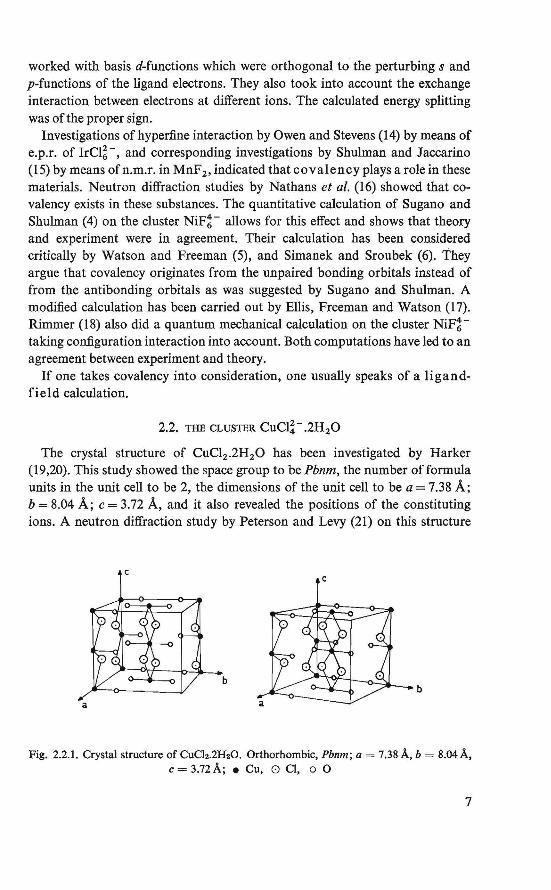
The crystal structure of CuC12 .2H20 has been investigated by Harker (19,20). This study showed the space group to be Pbnm, the number of formula units in the unit cell to be 2, the dimensions of the unit cell to be a = 7.38 A; b = 8.04 A; c = 3.72 A, and it also revealed the positions of the constituting ions. A neutron diffraction study by Peterson and Levy (21) on this structure
c c
b b
Fig. 2.2.1. Crystal structure of CuCb.2H20. Orthorhombic, Pbnm; a = 7.38 A, b = 8.04 A, c = 3.72 A; • Cu, o Cl, o o
7
has given about the same result, only the positions of the oxygen ions deviate slightly from those of the previous analysis. The neutron diffraction investigation also gives the proton sites. The result of this last structure analysis is shown in Fig. 2.2.1.
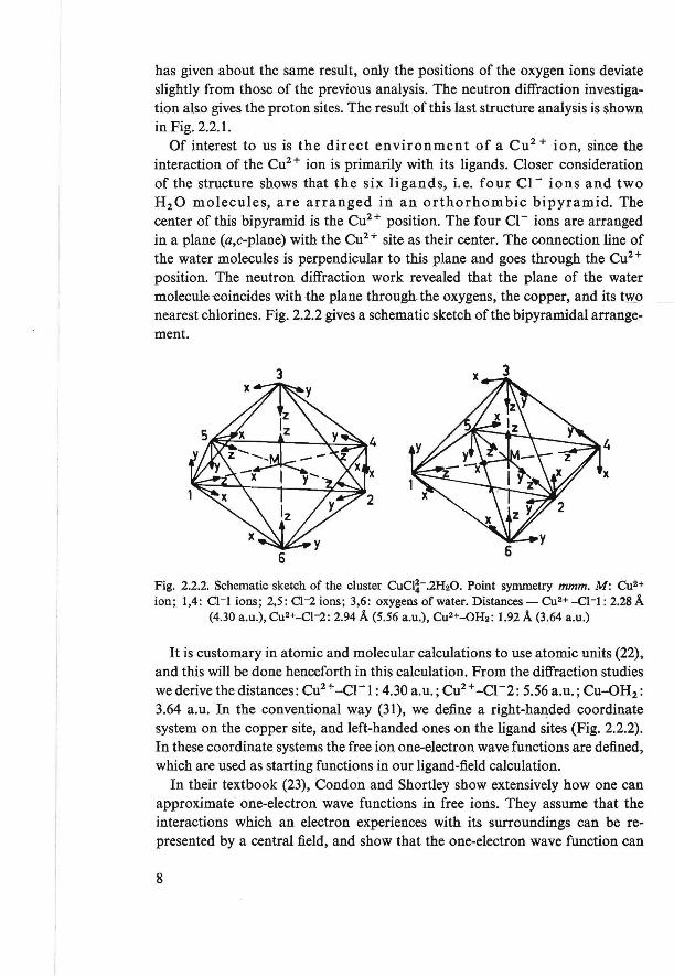
Of interest to us is the direct environment of a Cu2 + ion, since the interaction of the Cu2 + ion is primarily with its ligands. Closer consideration of the structure shows that the six ligands, i.e. four Cl - ions and two H 2 0 molecules, are arranged in an orthorhombic bipyramid. The center of this bipyramid is the Cu2 + position. The four c1- ions are arranged in a plane (a,c-plane) with the Cu2 + site as their center. The connection line of the water molecules is perpendicular to this plane and goes through the Cu2 +
position. The neutron diffraction work revealed that the plane of the water molecule -coincides with the plane through the oxygens, the copper, and its tw.o nearest chlorines. Fig. 2.2.2 gives a schematic sketch of the bipyramidal arrangement.
3
6
Fig. 2.2.2. Schematic sketch of the cluster CuCJ~-.2H20. Point symmetry mmm. M: eu2+ ion; 1,4: c1-1 ions; 2,5: Cl-Z ions; 3,6: oxygens of water. Distances- Cu2+-c1-1: 2.28 A
(4.30 a.u.), Cu2+-Cl-Z: 2.94 A (5.56 a.u.), Cu2+-0fü: 1.92 A (3.64 a.u.)
It is customary in atomie and molecular calculations to use atomie units (22), and this will be done henceforth in this calculation. From the diffraction studies we derive the distances: eu2 + -c1-1: 4.30 a.u.; Cu2+ -c1-2: 5.56 a.u.; Cu-OH2 :
3.64 a.u. In the conventional way (31), we define a right-handed coordinate system on the copper site, and left-handed ones on the ligand sites (Fig. 2.2.2). In these coordinate systems the free ion one-electron wave functions are defined, which are used as starting functions in our ligand-field calculation.
In their textbook (23), Condon and Shortley show extensively how one can approximate one-electron wave functions in free ions. They assume that the interactions which an electron experiences with its surroundings can be represented by a central field, and show that the one-electron wave function can
8
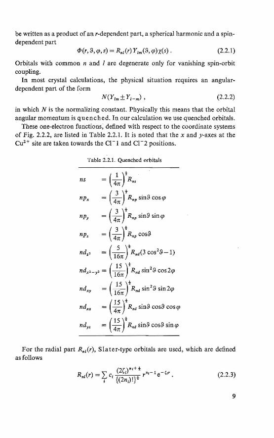
be written as a product of an r-dependent part, a spherical harmonie and a spindependent part
(2.2.1)
Orbitals with common n and l are degenerate only for vanishing spin-orbit coupling.
In most crystal calculations, the physical situation requires an angulardependent part of the form
(2.2.2)
in which N is the normalizing constant. Physically this means that the orbital angular momentum is quenched. In our calculation we use quenched orbitals.
These one-electron furictions; defined with respect to the coordinate systems of Fig. 2.2.2, are listed in Table 2.2.1. It is noted that the x and y-axes at the Cu2 + site are taken towards the Cl -1 and c1-2 positions.
Table 2.2.1. Quenched orbitals
ns = ( 4~ rR .. npx = ( :n rRnp sin.9 COS<p
npy = ( }n) t Rnp sin.9 sin <p
npz = ( :n rRnp cos.9
ndz2 = C~n r R.d(3 cos2.9-1)
ndx'-y' = ( ::n r Rnd sin2
.9 cos2<p
ndxy = ( 11:n r Rnd sin
2 8 sin 2<p
ndxz = ( !~ ) t Rnd sin.9 cos.9 cos <p
ndyz = ( !~ ) t Rnd sin.9 cos.9 sin <p
For the radial part R.1(r), Slater-type orbitals are used, which are defined as follows
(2.2.3)
9
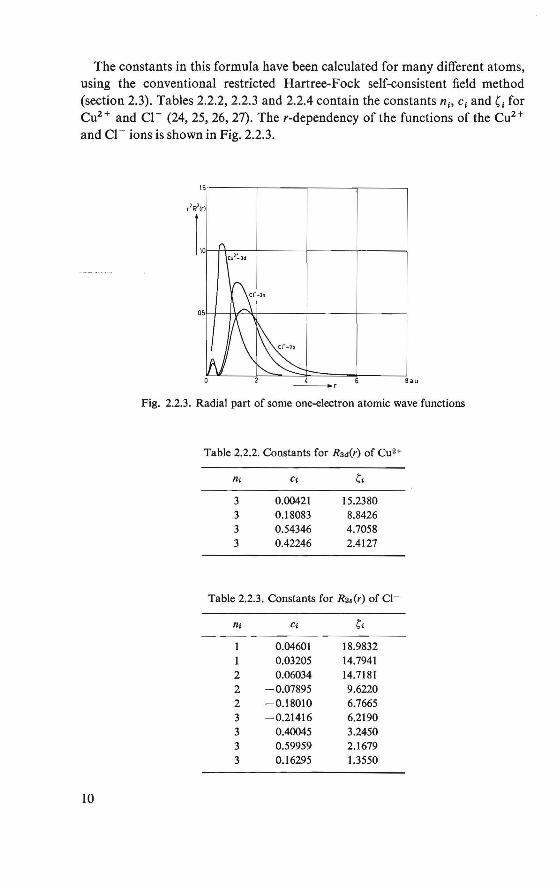
The constants in this formula have been calculated for many different atoms, using the conventional restricted Hartree-Fock self-consistent field method (section 2.3). Tables 2.2.2, 2.2.3 and 2.2.4 contain the constants ni, ei and C for Cu2 + and Cl - (24, 25, 26, 27). The r-dependency of the functions of the Cuz+ and Cl- ions is shown in Fig. 2.2.3.
10
l.Sc---~--~---~---
4 _, ea.u
Fig. 2.2.3. Radial part of some one-electron atomie wave functions
Table 2.2.2. Constants for Raii(r) of Cu2+
n1 Cl C1
3 0.00421 15.2380 3 0.18083 8.8426 3 0.54346 4.7058 3 0.42246 2.4127
Table 2.2.3. Constants for Rs,(r) of Cl-
rn C; C1
0.04601 18.9832 0.03205 14.7941
2 0.06034 14.7181 2 -0.07895 9.6220 2 -0.18010 6.7665 3 -0.21416 6.2190 3 0.40045 3.2450 3 0.59959 2.1679 3 0.16295 1.3550
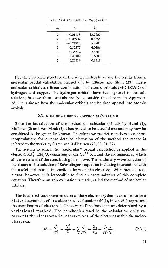
Table 2.2.4. Constants for Rsv(r) of Cl-
IU Cl Ct
2 -0.01158 13.7900 2 -0.03902 8.8355 2 -0.23912 5.3987 3 0.10277 4.0186 3 0.38612 2.4367 3 0.49189 1.6382 3 0.20319 0.8219
For the electronic structure of the water molecule we use the results from a molecular orbital calculation carried out by Ellison and Shull (28). These molecular orbitals are linear combinations of atomie orbitals (MO-LCAO) of hydrogen and oxygen. The hydrogen orbitals have been ignored in the calculation, because these orbitals are lying outside the cluster. In Appendix 2A. l it is shown how the molecular orbitals can be decomposed into atomie orbitals.
2.3. MOLECULAR ORBITAL APPROACH (MO-LCAO)
Since the introduction of the method of molecular orbitals by Hund (1), Mulliken (2) and Van Vleck (3) it has proved to be a useful one and may now be considered to be generally known. Therefore we restrict ourselves to a short recapitulation; for a more detailed discussion of the method the reader is referred to the works by Slater and Ballhausen (29, 30, 31, 32).
The system to which the "molecular" orbital calculation is applied is the cluster CuCii- .2H20, consisting of the Cu2 + ion and the six ligands, in which all the electrons of the constituting ions move. The stationary wave function of the electrons is a solution of Schrödinger's equation including interactions with the nuclei and mutual interactions between the electrons. With present techniques, however, it is impossible to find an exact solution of this complete equation. Therefore an approximation is made, called the method of molecular orbitals.
The total electronic wave function of the n-electron system is assumed to be a Sla ter determinant of one-electron wave functions i/t' (1), in which l represents the coordinates of electron 1. These wave functions then are determined by a
· variational method. The hamiltonian used in the calculation only represents the electrostatic in teractions of the electrons within the molecular system.
n v~ n z n 1 Jt= I --'+II-~+ I-,
t=I 2 a i=l ra.1 l<Jrlj (2.3.1)
11
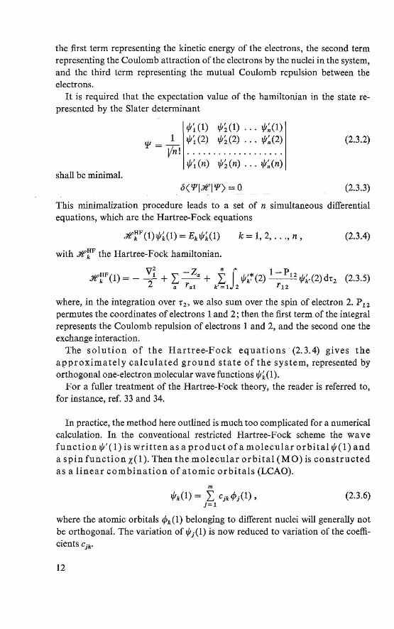
the first term representing the kinetic energy of the electrons, the second term representing the Coulomb attraction of the electrons by the nuclei in the system, and the third term representing the mutual Coulomb repulsion between the electrons.
It is required that the expectation value of the hamiltonian in the state represented by the Slater determinant
shall be minimal.
ifr~(l) iP;(l)." iP~(l) IJ' - _1 iP~ (2) iP; (2) . " iP~ (2)
- Vn1 .... .............. . iP~ (n) iP; (n) ... iP~(n)
<>< lJ'IYr'I P) = 0
(2.3.2)
(2.3.3)
This rninimalization procedure leads to a set of n simultaneous differential equations, which are the Hartree-Fock equations
Jr'~F (1) iP~(l) = Ed~(l)
with Jr'~F the Hartree-Fock hamiltonian.
k = 1, 2, ... , n,
Jr'~F(l)= - V2i + L -Za + f J iP~~(2) l-P12iP~· (2)dr2 " rai k' = 1 2 r 12
(2.3.4)
(2.3.5)
where, in the integration over r 2 , we also sum over the spin of electron 2. P 12
permutes the coordinates of electrons 1 and 2; then the first term of the integral represents the Coulomb repulsion of electrons 1 and 2, and the second one the exchange interaction.
The solution of the Hartree-Fock equations (2.3.4) gives the approximately calculated ground state of the system, represented by orthogonal one-electron molecular wave functions iP~(l).
Fora fuller treatment of the Hartree-Fock theory, the reader is referred to, for instance, ref. 33 and 34.
In practice, the method here outlined is much too complicated fora numerical calculation. In the conventional restricted Hartree-Fock scheme the wave function iP' ( 1) is wri tten as a product of a molecular orbi tal iP( 1) and a spin function x(l). Then the molecular orbi tal (MO) is constructed as a linear com bination of atomie orbitals (LCAO).
m
iPkCt) = 2: cjk<t>jU>, (2.3.6) j=l
where the atomie orbitals <f>k(l) belonging to different nuclei will generally not be orthogonal. The variation of iPJ{l) is now reduced to variation of the coefficients eik·
12
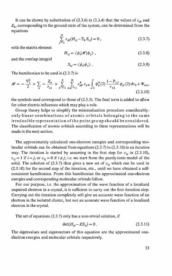
lt can be shown by substitution of (2.3.6) in (2.3.4) that the values of eik and Ek, corresponding to the ground state of the system, can be determined from the equations
m
(2.3.7)
with the matrix element (2.3.8)
and the overlap integral (2.3.9)
The hamiltonian to be used in (2.3. 7) is
VÎ " Z" ~ ~ * f * 1 - P 12 :Yé' ·=--2
+L,,--+ L,, L, Cpk'cp 'k' c/>p(2)--c/>p•(2)d-r2 +c!//0 xt> a ral k' = 1 p,p' = 1 2 r 12
(2.3.10)
the symbols used correspond to those of (2.3.5). The :final term is added to allow for other electric influences which may play a role.
Group theory helps to simplify the minimalization procedure considerably: only Jinear combinations of atomie orbitals belonging to the same irred uci bie represen tation of the point group should be co nsidered. The classi:fication of atomie orbitals according to these representations will be made in the next section.
The approximately calculated one-electron energies and corresponding molecular orbitals can be obtained from equations (2.3.7) to (2.3.10) in an iterative way. The iteration is started by assurning in the first step for c1i in (2.3.10), cu = 1 if i = j, or c1i = 0 if i # j; i.e. we start from the purely ionic model of the solid. The solution of (2.3.7) then gives a new set of c1i which can be used in (2.3.10) for the second step of the iteration, etc., until we have obtained a selfconsistent hamiltonian. From this hamiltonian the approximated one-electron energies and corresponding molecular orbitals follow.
For our purpose, i.e. the approximation of the wave function of a localized unpaired electron in a crystal, it is sufficient to carry out the first iteration step. Carrying out the iteration completely will give an accurate wave function of an electron in the isolated cluster, but not an accurate wave function of a localized electron in the crystal.
The set of equations (2.3.7) only has a non-trivial solution, if
(2.3.11)
The eigenvalues and eigenvectors of this equation are the approximated oneelectron energies and molecular orbitals respectively.
13
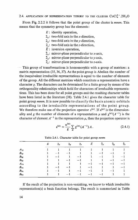
2.4. APPLICATION OF REPRESENTATION THEORY TO THE CLUSTER CuCli-.2H20
From Fig. 2.2.2 it follows that the point group of the cluster is mmm. This means that the symmetry group has the elements:
E : identity operation, 2x: two-fold axis in the x-direction, 2y: two-fold axis in the y-direction, 2z: two-fold axis in the z-direction, Ë : inversion operation, Ïx: mirror-plane perpendicular to x-axis, Ïy: mirror-plane perpendicular to y-axis, Ïz: mirror-plane perpendicular to z-axis.
-- This group of transformations is homomorphic with a group of matrices: a matrix representation (35, 36, 37). As the point group is Abelian the number of the inequivalent irreducible representations is equal to the number of elements of the group. All the different matrices which constitute a representation have a character X· The characters can be determined fora finite group by means of the orthogonality relationships which hold for characters of irreducible representations. This has been done for all point groups and the resulting character tables have been Iisted in the Iiterature (38). Table 2.4.1 gives the character table for point group mmm. lt is now possible to classify the basis atomie orbitals according to the irreducible representations of the point group. We therefore make use of the projection operator e<µ). If n<µJ is the dimensionality and g the number of elements of a representation µand x<µl(A- 1
) is the character of element A - 1 in the representation µ, then the projection operator is
À1g
Bio B2o Bag
A1u
B1u B2u Bsu
(µ)
e<µ> =~:Lx<µ>(A- 1)A. g A
Table 2.4.1 . Character table for point group mmm
E 2z 2y 2, 2"
1 1 -1 -1 -1 -1 -1 -1
-1 -1 1 -1 -1
-1 -1 -1 -1 1 -1 -1 1
-1 -1 -1 -1
(2.4.1)
2u
-1 1 -1
-1 -1 -1 -1
-1 -1 1
1
If the result of the projection is non-vanishing, we know to which irreducible representation(s) a basis function belongs. The result is summarized in Table
14
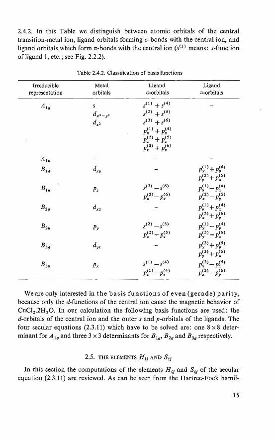
2.4.2. In this Table we distinguish between atomie orbitals of the central transition-metal ion, ligand orbitals fonning u-bonds with the central ion, and ligand orbitals which form n-bonds with the central ion (s< 1 > means: s-function of ligand 1, etc.; see Fig. 2.2.2).
Table 2.4.2. Classification of basis functions
Irreducible Metal Ligand Ligand representation orbitals a-orbitals n-orbitals
À1g s s<I) + s<4>
dx2-y2 s<2> + s<S>
dzl 5(3) + s<6)
p;1) + p;4) p;2) + p~5) p~3) + p~6)
A1u
B1u dxy p~l) + p~4) p~2)+ p~S)
B1u Pz s<J> -s<6> p~l)_ p~4}
p~3)_ p;6) p~2)_ p~5)
B2u dxz p~l)+ p~4)
p~3)+ p~6)
B2. Py s<2) _ 5(5) p~l)_ p~4)
p~2)_ p;s> p~3)_ p~6)
B3u dyz p~2)+ p~S)
p~3) + p~6)
B3u Px s<I) -s<4> p~2)_ p~S)
p~l)-p~4) p~3)_ p~6)
We are only interested in the basis functions of even (gerade) pari ty, because only the d-functions of the centra! ion cause the magnetic behavior of CuCl2 .2H20. In our calculation the following basis functions are used: the d-orbitals of the central ion and the outer s and p-orbitals of the ligands. The four secular equations (2.3.11) which have to be solved are: one 8 x 8 determinant for A 19 and three 3 x 3 determinants for B 19, B29 and B39 respectively.
2.5. THE ELEMENTS Hij AND Sij
In this section the computations of the elements HiJ and SiJ of the secular equation (2.3.11) are reviewed. As can be seen from the Hartree-Fock hamil-
15
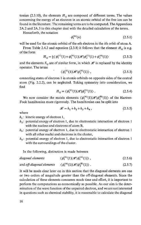
tonian (2.3.10), the elements HIJ are composed of different terms. The values concerning the energy of an electron in an atomie orbi tal of the free ion can be found in the literature. The remaining terms are to be computed. The Appendices 2A.2 and 2A.3 to this chapter deal with the detailed calculation of the terms.
Henceforth, the notation (2.5.1)
will be used for the atomie orbital of the nth electron in the ith or bit of atom A. From Table 2.4.2 and equation (2.3.8) it follows that the element Hii is e.g.
of the form (2.5.2)
and the elements Sii are of similar form, in which :lf is replaced by the identity operator. The terms
(2.5.3)
connecting states of electron l in atomie orbitals on opposite si des of the centra} atom (Fig. 2.2.2), can be neglected. Taking symmetry into consideration, we find
(2.5.4)
We now consider the matrix elements (</>lA)(l)l:lfl</>)Bl(l)) of the HartreeFock hamiltonian more rigorously. The hamiltonian can be split into
(2.5.5) where h1 : kinetic energy of electron 1, h2 : potential energy of electron l, due to electrostatic interaction of electron 1
with the nucleus and electrons of atom B, h3 : potential energy of electron l, due to electrostatic interaction of electron 1
with all other nuclei and electrons in the cluster, h4 : potential energy of electron 1, due to electrostatic interaction of electron 1
with the surroundings of the cluster.
In the following, distinction is made between
diagonal elements (</>~Al(l)l:lfl</>lA)(l)),
and off-diagonal e/ements (</>lA)(l)l:lfl</>)Bl(l)).
(2.5.6)
(2.5.7)
lt will be made clear later on in this section that the diagonal elements are one or two orders of magnitude greater than the off-diagonal elements. Since the calculation of these elements consumes much time and effort, it is important to perform the computations as economically as possible. As our aim is the determination of the wave function of the unpaired electron, and we are not interested in questions such as chemica! stability, it is reasonable to calculate the diagonal
16
elements accurately and leave some uncertainty in the off-diagonal elements by making an approximation.
DIAGONAL ELEMENTS
These elements can be split in two different types:
one-center integrals, elements with h1 and h2 ,
two-center integrals, elements with h3 and h4 .
One-center integrals As we have seen h1 +h2 gives the energy of an electron in the free ion state.
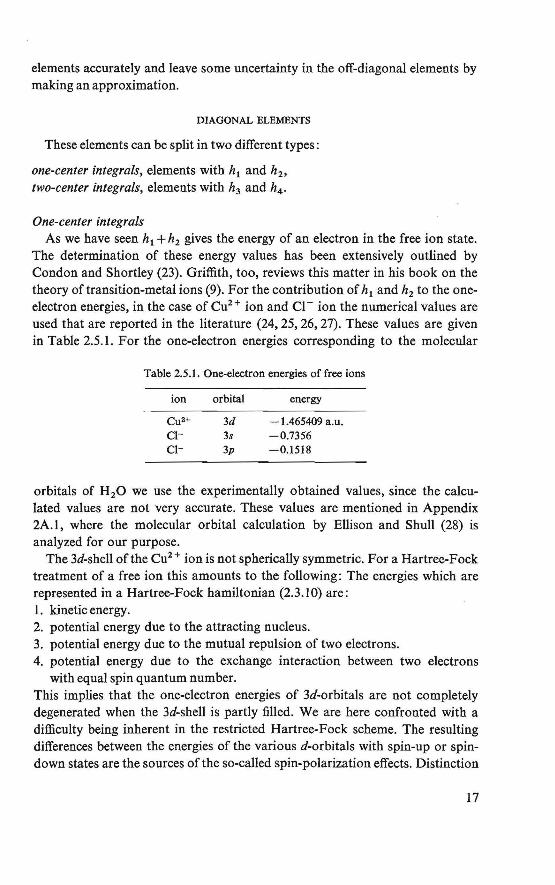
The determination of these energy values has been extensively outlined by Condon and Shortley (23). Griffith, too, reviews this matter in his book on the theory of transition-metal ions (9). For the contribution of h1 and h2 to the oneelectron energies, in the case of Cu2 + ion and ei- ion the numerical values are used that are reported in the literature (24, 25, 26, 27). These values are given in Table 2.5.1. For the one-electron energies corresponding to the molecular
Table 2.5.1. One-electron energies of free ions
ion orbital energy
Cu2+ 3d -1.465409 a.u. a- 3s -0.7356 c1- 3p -0.1518
orbitals of H 20 we use the experimentally obtained values, since the calculated values are not very accurate. These values are mentioned in Appendix 2A. l, where the molecular orbital calculation by Ellison and Shull (28) is analyzed for our purpose.
The 3d-shell of the Cu2 + ion is not spherically symmetrie.Fora Hartree-Fock treatment of a free ion this amounts to the following: The energies which are represented in a Hartree-Fock hamiltonian (2.3.10) are: 1. kinetic energy. 2. potential energy due to the attracting nucleus. 3. potential energy due to the mutual repulsion of two electrons. 4. potential energy due to the exchange interaction between two electrons
with equal spin quantum number. This implies that the one-electron energies of 3d-orbitals are not completely degenerated when the 3d-shell is partly filled. We are here confronted with a difficulty being inherent in the restricted Hartree-Fock scheme. The resulting differences between the energies of the various d-orbitals with spin-up or spindown states are the sources of the so-called spin-polarization effects. Distinction
17
between different spin-states would render our calculation much more complicated. We shall not consider this problem here, but deal with it in Appendix 2A.2.
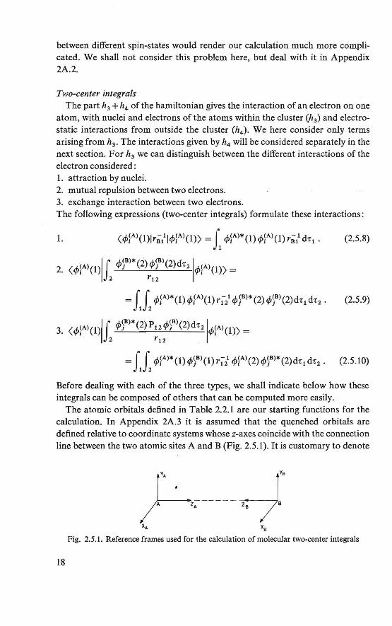
Two-center integrals The part h3 + h4 of the hamiltonian gives the interaction of an electron on one
atom, with nuclei and electrons of the atoms within the cluster (h3) and electrostatic interactions from outside the cluster (h4 ). We here consider only terms arising from h3 • The interactions given by h4 will be considered separately in the next section. For h3 we can distinguish between the different interactions of the electron considered : 1. attraction by nuclei. 2. mutual repulsion bet ween two electrons. 3. exchange interaction between two electrons. The following expressions (two-center integrals) formulate these interactions:
<4>fA)(l)lr8/14>fAl(l)) = f1 4>fAl*(l)</>fAl(l)r8/dt1.
2. <4>~Al(l)IJ 4>)B>*(2)</>)s>(2)dt214>lA>(1)) = 2 '12
1. (2.5.8)
= JJ2
</>fA)*(l)</>[A\l)r1-/4>JB)*(2)</>)8 )(2)dt1dt2. (2.5.9)
3. <4>lA>(1)IJ 4>)B>*(2)P124>)sl(2)dt214>lA>(1)) =
2 '12
Before dealing with each of the three types, we shall indicate below how these integrals can be composed of others that can be computed more easily.
The atomie orbitals defined in Table 2.2.1 are our starting functions for the calculation. In Appendix 2A.3 it is assumed that the quenched orbitals are defined relative to coordinate systems whose z-axes coincide with the connection line between the two atomie sites A and B (Fig. 2.5.1). It is customary to denote
f-ç-----~-~I ~ ~
Fig. 2.5.1. Reference frames used for the calculation of molecular two-center integrals
18
the quenched orbitals in this reference frame by (Fig. 2.5.1) s: s11; Pz: p11; Px.Py: pn; dz,: d11; dx"dyz: dn; dx2-yi, dxy: dö . In genera! (Fig. 2.2.2) the starting functions are not defined in such a frame. We, therefore, have to transform the original functions into a sum of 11, n, and ó-functions. lt can be shown by simpte algebra how the transformation can be performed (31,39). It then also fellows how the integrals which we want to calculate can be composed of the simpler ones, that have been calculated in the transformed reference frame (Fig. 2.5.1). lt is furthermore convenient for the calculation of Coulomb and exchange integrals, to decompose the angular-dependent part of the quenched orbitals in to spherical harmonies (2.2.2); then the integrals are computed for atomie functions having a spherical harmonie as angular-dependent part.
In Appendix 2A.3 the two-center integrals (2.5.8), (2.5.9), (2.5.10) are converted into a form which can be programmed for an electronic computer. The integrals (2.5.8) and (2.5.10) were programmed in Fortran to be computed on the IBM 1620 of the Mathematics Department of this University. The integrals (2.5.9) were programmed in Algol for calculation on the TR 4 of the Mathematics Department of the Technologica! University of Delft.
Nuclear attraction integrals: The numerical values of these integrals can readily be obtained for various cases by applying the formulae derived in Appendix 2A.3. The results of these calculations are summarized in Table 2.5.2.
Coulomb repulsion and exchange interaction integrals: For the d-functions of the Cul+ ion the Coulomb and exchange interaction integrals for the interaction with the outer ligand functions have been calculated (the 3p-functions of c1-and the 2p-functions of oxygen in H20). Only those integrals have to be calculated in which the azimuthal quantum numbers obey the relation
for the Coulomb repulsion integrals, or
for the exchange interaction integrals. The results of the computations are given in Table 2.5.3.
OFF-DIAGONAL ELEMENTS
lt is here discussed how the numerical values of the integrals
(2.5.7)
are obtained. In our calculation we use one-electron wave functions of free ions, which have been obtained from a restricted Hartree-Fock calculation. We
19
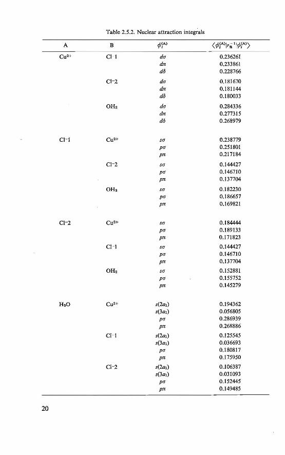
Table 2.5.2. Nuclear attraction integfals
A B rp'('> < r/J'f'>lriï 1lr/J'f'>) eu2+ c1-1 drJ 0.236261
dn 0.233861 do 0.228766
c1-2 drJ 0.181670 dn 0.181144 do 0.180033
OH2 drJ 0.284336 dn 0.277315 do 0.268979
c1-1 Cu2+ S(] 0:238779 PrJ 0.251801 p1'l 0.217184
c1-2 S(] 0.144427 prJ 0.146710 p1'l 0.137704
OH2 S(] 0.182230
PrJ 0.186657 p1'l 0.169821
c1-2 Cu2+ S(] 0.184444 prJ 0.189133 p1'l 0.171823
c1-1 SrJ 0.144427 prJ 0.146710 p1'l 0.137704
Ofü S(] 0.152881
PrJ 0.155752 p1'l 0.145279
H20 Cu2+ s(2a1) 0.194362 s(3a1) 0.056805
prJ 0.286939 p1'l 0.268886
c1-1 s(2a1) 0.125545 s(3a1) 0.036693
prJ 0.180817 p1'l 0.175950
c1-2 s(2a1) 0.106387 s(3a1) 0.031093
prJ 0.152445 p1'l 0.149485
20
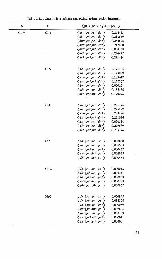
Table 2.5.3. Coulomb repulsion and exchange interaction integrals
A B < ef>(l)f lef>* (2)rl21ef>(2)f lef>(l))
Cu2+ c1-1 <da [pa pa [da) 0.254453 <da fpnpn Ida) 0.218649 (dn*[pa pa [dn±) 0.250878 <dn+[pn+pn+\dn+) 0.217060 < dn+ 1 pn-pn- f dn+ > 0.000338 <dö±[pa pa [do*) 0.244472 (dö± [pn±pn± 1 dö±) 0.213444
c1-2 (da jpa pa 1 da ) 0.191165 <da [pn±pn±jda) 0.173099 (dn*fpa pa [dn±) 0.189647 < dn+ 1 pn+pn+ 1 dn+ > 0.172267 (dn+ jpn-pn-j dn+) 0.000121 (dö±jpa pa jdö±) 0.186566 (dö± jpn±pn±j dö±) 0.170298
H20 (da jpa pa Ida) 0.296374 (da [pn±pn± 1 da ) 0.275292 (dn±[pa pa [dn±) 0.289474 (dn+fpn+pn+\dn+) 0.271076 (dn+jpn-pn-jdn+) 0.000334 ( dö± jpa pa 1 dö±) 0.279589 <do± lpn±pn± 1 do±) 0.263774
c1-1 (da 1 sa da 1 sa ) 0.000630 (da jpa da jpa ) 0.006705 <da jpn*da jpn±) 0.000467 (dn" [pa dn± jpa ) 0.002065 (dö±jpa do"fpa ) 0.000482
c1-2 <da 1 sa da 1 sa ) 0.000018 <da jpa da jpa ) 0.000441 (da jpn±da jpn±) 0.000088 (dn±jpa dn±jpa > 0.000188 <do±jpa dö±fpa) 0.000057
H20 (da 1 sa da 1 sa ) 0.000995 (da [pa da jpa ) 0.014226 (da \pn±da jpn±) 0.000059 <dn±jpa dn±[pa) 0.002624 (dö±jpa dö±fpa > 0.000183 <dn+jpn+dn+[pn+) 0.000011 <dn+ jpn-dn+ jpn-) 0.000001
21
assume that these wave functions are eigenfunctions of the self-consistent Hartree-Fock hamiltonian.
(2.5.11)
Then, for Ei we take the one-electron energies which we also used in the calculation of the diagonal elements. Hence
(2.5.12)
The remaining part
(2.5.13)
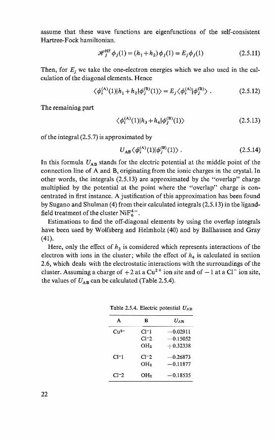
of the integral (2.5.7) is approximated by
U AB(<p~A)(l)lcf>)Bl(l)). (2.5.14)
In this formula UAB stands for the electric potential at the middle point of the connection line of A and B, originating from the ionic charges in the crystal. In other words, the integrals (2.5.13) are approximated by the "overlap" charge multiplied by the potential at the point where the "overlap" charge is concentrated in first instance. A justification of this approximation bas been found by Sugano and Shulman ( 4) from their calculated integrals (2.5.13) in the ligandfield treatment of the cluster NiF~-.
Estimations to find the off-diagonal elements by using the overlap integrals have been used by Wolfsberg and Helmholz (40) and by Ballhausen and Gray (41).
Here, only the effect of h3 is considered which represents interactions of the electron with ions in the cluster; while the effect of h4 is calculated in section 2.6, which deals with the electrostatic interactions with the surroundings of the cluster. Assuming a charge of+ 2 at a Cu2 + ion site and of - 1 at a ei- ion site, the values of U AB can be calculated (Table 2.5.4).
Table 2.5.4. Electric potential U AB
A B UAB
Cu2+ c1-1 -0.02911 c1-2 -0.15052 OH2 +0.32338
c1-1 c1-2 -0.26873 OH2 -0.11877
cr--i OH2 -0.18535
22
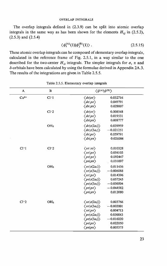
OVERLAP INTEGRALS
The overlap integrals defined in (2.3.9) can be split into atomie overlap integrals in the same way as bas been shown for the elements Hu in (2.5.2), (2.5.3) and (2.5.4)
(2.5.15)
These atomie overlap integrals can be composed of elementary overlap integrals, calculated in the reference frame of Fig. 2.5. l, in a way similar to the one described for the two-center H 11 integrals. The simpler integrals for a, n and 8-orbitals have been calculated by using the formulae derived in Appendix 2A.3. The results of the integrations are given in Table 2.5.5.
Table 2.5.5. Elementary overlap integrals
A B < <j>!All<f>!B>)
Cu2+ c1-1 (dulso) 0.032716 (dulpu) 0.049791 (dnlpn) 0.028007
(dulsu) 0.008548 (dulpu) 0.019531 (dnJpn) 0.008777
( duls(2ai)) 0.039959 ( duJs(3a1)) -0.021251 (duJpu) 0.059791 (dnJpn) 0.026006
(salsa) 0.010328 (sulpu) 0.054103 (pulpa) 0.092447 (pnlpn) 0.031097
Ofü (sa ls(2a1)) 0.011456 (sa ls(3a1)) -0.006088 (sulpu) 0.014396 (puJs(2a1)) 0.057245 (puls(3a1)) -0.030504 (pulpa) -0.044582 (pnlpn) 0.012080
Ofü (suJs(2a1)) 0.003766 (sa ls(3a1)) -0.002001 (sulpu) 0.004713 (puls(2a1)) 0.030063 (puJs(3a1)) -0.016020 (pulpa) 0.022050 (pnlpn) 0.005375
23
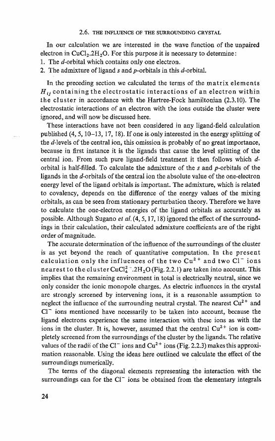
2.6. THE INFLUENCE OF THE SURROUNDING CRYSTAL
In our calculation we are interested in the wave function of the unpaired electron in CuC12 .2H20. For this purpose it is necessary to detennine: 1. The d-orbital which contains only one electron. 2. The admixture of ligand s and p-orbitals in this d-orbital.
In the preceding section we calculated the terms of the matrix elements Hli containing the electrostatic interactions of an electron within the cluster in accordance witb the Hartree-Fock bamiltonian (2.3.10). The electrostatic interactions of an electron with the ions outside the cluster were ignored, and will now be discussed here.
These interactions have not been considered in any ligand-field calculation published (4, 5, 10-13, 17, 18). If one is.only interested in the energy splitting of the d-levels of the central ion, this omission is probably of no great importance, because in first instance it is the ligands that cause the level splitting of the centra! ion. From such pure ligand-field treatment it then follows which dorbital is half-filled. To calculate the admixture of the s and p-orbitals of the ligands in the d-orbitals of the central ion the absolute value of the one-electron energy level of the ligand orbitals is important. The admixture, which is related to covalency, depends on the difference of the energy values of the mixing orbitals, as can be seen from stationary perturbation theory. Tberefore we have to calculate the one-electron energies of the ligand orbitals as accurately as possible. Although Sugano et al. (4, 5, 17, 18) ignored the effect of the surroundings in their calculation, their calculated admixture coefficients are of the right order of magnitude.
The accurate determination of the influence of the surroundings of the cluster is as yet beyond the reach of quantitative computation. In the present calculation only the influences of the two Cu2 + and two Cl - ions nearest to the cluster CuCl~- .2H20 (Fig. 2.2.1) are taken into account. This implies that the remaining environment in total is electrically neutra!, since we only consider the ionic monopole charges. As electric influences in the crystal are strongly screened by intervening ions, it is a reasonable assurnption to neglect the infiuence of the surrounding neutra! crystal. The nearest Cu2 + and ei- ions mentioned have necessarily to be taken into account, because the ligand electrons experience the same interaction with these ions as with the ions in the cluster. It is, however, assumed that the centra! Cu2+ ion is completely screened from the surroundings of the cluster by the ligands. The relative values of the radii of the Cl - ions and Cu2 + ions (Fig. 2.2.3) makes this approximation reasonable. Using the ideas here outlined we calculate the effect of the surroundings numerically.
The terms of the diagonal elements representing the interaction with the surroundings can for the ei- ions be obtained from the elementary integrals
24
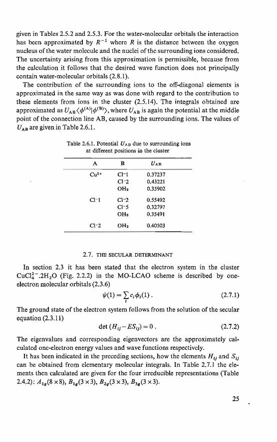
given in Tables 2.5.2 and 2.5.3. For the water-molecular orbitals the interaction has been approximated by R- 1 where R is the distance between the oxygen nucleus of the water molecule and the nuclei of the surrounding ions considered. The uncertainty arising from this approximation is permissible, because from the calculation it follows that the desired wave function does not principally contain water-molecular orbitals (2.8.1).
The contribution of the surrounding ions to the off-diagonal elements is approximated in the same way as was done with regard to the contribution to these elements from ions in the cluster (2.5.14). The integrals obtained are approximated as UAB (</><All<f/ 8 >), where UAB is again the potential at the middle point of the connection line AB, caused by the surrounding ions. The values of UAa are given in Table 2.6.1.
Table 2.6.1. Potential U AB due to surrounding ions at different positions in the cluster
A B UAB
Cu2+ c1-1 0.37237 c1-2 0.43221 OH2 0.35902
c1-2 0.55492 c1-5 0.32797 OH2 0.35491
OH2 0.40503
2. 7. THE SECULAR DETERMINANT
In section 2.3 it has been stated that the electron system in the cluster CuCI!- .2H20 (Fig. 2.2.2) in the MO-LCAO scheme is described by oneelectron molecular orbitals (2.3.6)
1/1(1) = ~::Ci</>1(1). (2.7.1) 1
The ground state of the electron system follows from the solution of the secular equation (2.3.11)
(2.7.2)
The eigenvalues and corresponding eigenvectors are the approximately calculated one-electron energy values and wave functions respectively.
It has been indicated in the preceding sections, how the elements Hli and Sli can be obtained from elementary molecular integrals. In Table 2.7.1 the elements then calculated are given for the four irreducible representations (Table 2.4.2): A19 (8 x8), B19 (3 x3), B2g(3 x3), B3g(3 x3).
25
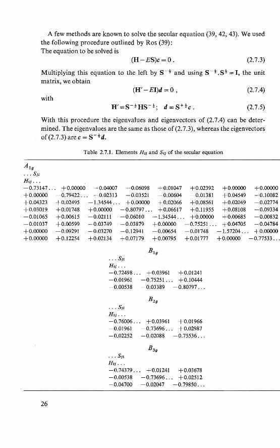
A few methods are known to solve the secular equation (39, 42, 43). We used the following procedure outlined by Ros (39): The equation to be solved is
(H-ES)c = 0. (2.7.3)
M ultiplying this equation to the left by s - t and using S - t. S t = 1, the unit matrix, we obtain
(H'-El)d = 0 , (2.7.4) with
(2.7.5)
With this procedure the eigenvalues and eigenvectors of (2.7.4) can be determined. The eigenvalues are the same as those of (2. 7.3), whereas the eigenvectors of(2.7.3) are c = s-td.
À1g
. •• S 11
H 11 •. .
- 0.73147 ... +0.00000 +0.04323 + 0.03019 -0.01065 - 0.01037 + 0-.00000 + 0.00000
26
Table 2.7.1. Elements H 11 and S11 of the secular equation
+0.00000 -0.79422 ... +0.02495 +0.01748 +0.00615 +0.00599 -0.09291 +0.12254
-0.04007 -0.06098 +0.01047 +0.02392 -0.02313 -0.03521 -0.00604 -0.01381
-1.34544 . . . +0.00000 +0.02066 +0.08561 +0.00000 -0.80797 .. . +0.06617 +0.11955 -0.02111 -0.06010 -1.34544 . .. +0.00000 -0.03749 -0.03879 + 0.00000 - 0.75251 ... -0.03270 -0.12941 - 0.00654 -0.01748 +0.02134 +0.07179 +0.00795 +0.01777
Big
• . • S11
H11 .. .
-0.72498 ... + 0.03961 +0.01241 - 0.01961 -0.00538
... s,, H11 . •.
-0.76006 .. . - 0.01961 - 0.02252
... s" H11 .••
-0.75251 ... + 0.10444 -0.03389 -0.80797 . . .
B2g
+ o.03961 + 0.01966 -0.73696 ... + 0.02987 -'--0.02088 -0.75536 . ..
B3g
- 0.74379... + 0.01241 +0.03678 -0.00538 -0.73696. .. + 0.02512 -0.04700 - 0.02047 -0.79850 . ..
+0.00000 +0.04549 + 0.02049 +0.08108 +0.00685 +0.04705
-1.57204 .. . +0.00000
+0.00000 -0.10082 -0.02774 -0.09334 -0.00832 - 0.04784 +0.00000
-0.77533 ...
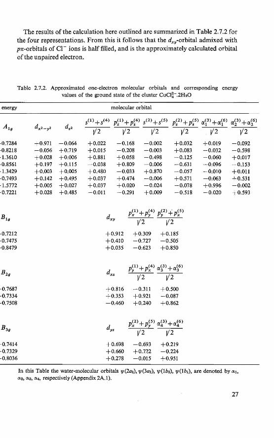
The results of the calculation here outlined are summarized in Table 2.7.2 for the four representations. From this it follows that the dxy-orbital admixed with pn-orbitals of Cl - ions is half filled, and is the approximately calculated orbi tal of the unpaired electron.
Table 2.7.2. Approximated one-electron molecular orbitals and corresponding energy values of the ground state of the cluster CuCJ~-.2H20
energy
·0.7284 -0.8218 · l.3610 ·0.8561 · l.3429 -0.7493 ·l.5772 ·0.7221
·0.7212 ·0.7475 ·0.8479
-0.7687 -0.7334 -0.7508
-0.7414 -0.7329 -0.8036
dx2-y2 dz2
+0.971 -0.064 -0.056 +0.719 +0.028 +0.006 +0.197 +0.115 +0.003 +0.005 +0.142 +0.495 +0.005 +0.027 +0.028 +0.485
rnolecular orbital
s<1> + s<4> p;1>+ P;4> s<2>+s<s> p;2> + p~s> a13) +a16)
v2 v2 v2 v2 +0.022 -0.168 -0.002 +0.032 +0.015 -0.208 -0.003 +0.083 +0.881 +0.058 -0.498 -0.125 -0.038 +0.809 -0.006 -0.631 +0.480 -0.033 +0.870 -0.057 +0.037 +0.474 -0.006 +0.571 +0.037 +0.020 -0.024 -0.078 -0.011 -0.291 +0.009 -0.518
dxy p~l) + p~4) p~2) + p~S)
v2 v2 +0.912 +o.309 +0.185 +0.410 -0.727 -0.505 +0.035 -0.623 +0.850
dxz P~1> + P~4> a~3> +a~6>
v2 v2 +0.816 -0.311 +0.500 +0.353 +0.921 -0.087 -0.460 +0.240 +0.862
p~2) + p~s> a1_3l + ai6l
v2 v2 +0.698 -0.693 +0.219
-0.224 +0.951
+o.660 +o.n2 +0.278 -0.015
v2 +0.019 -0.032 -0.060 -0.096 -0.010 -0.063 +0.996 -0.020
a~3) +a~6>
v2 -0.092 -0.598 +0.017 -0.153 +0.011 +0.531 -0.002 +0.593
In this Table the water-molecular orbitals 1/1(2a1), 1/1(3a1), VJ(lb2), 1/l(lb1), are denoted by 0:1, 0:2, ixs, lX4, respectively (Appendix 2A.l).
27
2.8. DISCUSSION AND CONCLUSION
The approximately calculated orbi tal of the unpaired electron is
(2.8.1)
We conclude from this that the admixtures of the d-orbitals are pn-orbitals of the chlorine ions only, hence the con:figuration of this molecular orbital is planar. This approximated orbital will be used in the following as the spacedependent part of the total wave function of the unpaired electron.
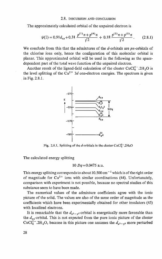
Another result of the ligand-field calculation of the cluster CuCl~ - .2H20 is the level splitting of the Cu2 + 3d one-electron energies. The spectrum is given in Fig. 2.8.1.
-0.70
E /dxy
î-~74 \:d'!'2 l d,2 y2
\;Ji~ 100q
! 32
-0.78 du
-0.82 d(I) z2
Fig. 2.8.1. Splitting of the d-orbitals in the cluster CuCI~-.2füO
The calculated energy splitting
10 Dq=0.0475 a.u.
This energy splitting corresponds to about 10.500 cm - t which is of the right order of magnitude for Cu2+ ions with similar coordinations (44). Unfortunately, comparison with experiment is not possible, because no spectra! studies of this substance seem to have been made.
The numerical values of the admixture coefficients agree with the ionic picture of the solid. The values are also of the same order of magnitude as the coefficients which have been experimentally obtained for other insulators (45) with localized electrons.
It is remarkable that the dx>-yi-orbital is energetically more favorable than the dxy-orbital. This is not expected from the pure ionic picture of the cluster CuCI!- .2H20, because in this picture one assumes the dx>- 11 more perturbed
28
by the point charges at the chlorine sites than the d-"Y-orbitals, since the lobes of the d:c2- y2 point towards the negative charges, while the d-"Y are in between. This is indeed found if only allowance is made for the Coulomb repulsion of the electron. However, the energy lowering owing to the exchange interaction causes the total one-electron energy of the d:c2- yz-orbital to be lower than that of the dxy-orbital.
The results of a recent investigation carried out by O'Sullivan, Simmons and Roberts (46, 47) on magnetic resonance of the chlorine nuclei, shows that the values they found for the admixture coefficients from the hyperfine interactions are of the same order of magnitude as the ones we calculated. They assumed that the dx•- yz-orbital is half filled, which is probably incorrect, and interpreted their results in accordance with this assumption. They also showed that this assumption is in accordance with their nuclear quadrupole resonance results. This interpretation, however, is based on the assumption that the ions in the solid can be replaced by point charges, which likely is too simple an assumption.
APPENDIX 2A.1 ANALYSIS OF A MOLBCULAR ORBITAL CALCULATION OF WATER
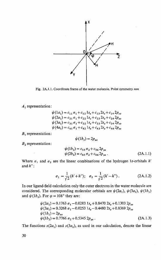
From the neutron diffraction data (21) we know that the nuclei of the water molecule lie in a plane, which coincides with the horizontal plane in Fig. 2.2.2. These data also show that the angle <p between the connection lines of the protons with the oxygen nucleus is 108°. This suggests that the water molecule in the solid is not strongly modified by its surroundings. Schematically, this horizontal plane looks as shown in Fig. 2A.1. l.
The molecular orbitals resulting from the calculation carried out by Ellison and Shull, will be analyzed for adaptation to our calculation. On account of the limited spatial distribution of the hydrogen orbitals, these atomie orbitals are ignored. Then the overlap of the starting orbitals in our calculation with the water-molecular orbitals is only due to that part of the molecular orbital centered around the oxygen site. The energy values corresponding to the molecular orbitals are taken from this treatment.
The point group of the symmetry of the water molecule is mm. We can distinguish four different irreducible representations of the group. From the molecular orbital calculation it follows that only the A1 , B1 and B 2 representations are relevant. According to Ellison and Shull's calculation the following linear combinations of atomie oxygen and hydrogen orbitals are possible within these representations.
29
x
H
z
Fig. 2A. l .1. Coordinate frame of the water molecule. Point syrnmetry mm
A 1 representation:
B 1 representation:
B2 representation:
l/J(la1) = c11 u1 +c12 ls0 +c13 2s0 +c14 2P:,,0
l/1(2a1) = C21 Ui +c22 lso+C232so+c242pzo l/1(3a1) = C3i u 1 +c32 ls0 +C332s0 +C342p,0
l/J(4a1) = C41 U1 +c42 lso +c43 2so +c44 2Pzo
l/J(lb2) = C55 U2 + Cs6 2pyo l/1(2b2) = C6s U2 + c66 2Pyo · (2A.1.1)
Where ui and u2 are the linear combinations of the hydrogen ls-orbitals h' and h":
""1 = /2
(h' +h"); a2 = / 2 (h'-h"). (2A.1.2)
In our ligand-:field calculation only the outer electrons in the water molecule are considered. The corresponding molecular orbitals are l/J(2a1), l/J(3ai), l/J(lb1) and l/J(lh2). For <p = 108° they are:
l/1(2a1) = 0.1763 u1 -0.0283 ls0 +0.8470 2s0 +0.1303 2Pzo l/1(3ai) = 0.3268 Ui -0.0253 ls0 -0.4480 2s0 +0.8369 2Pzo
l/J(lb1) = 2Pxo l/I (lb2) = 0. 7766 u 2 + 0.5345 2Pya . (2A.1.3)
The functions s(2ai) and s(3ai), as used in our calculation, denote the linear
30
combinations of the Is and 2s-atomic functions in 1/1(2a1) and l/f (3a1) respectively.
Ellison and Shull used Slater atomie functions </>0 with radial dependence
R (r) = (20"+t r"-1e-çr n {(2n)!}t
The constants they used are given in Table 2A. l. l.
Table 2A.l.l. Rn(r) of oxygen
Is 2s 2p
n
2 2
-7.700 -2.275 -2.275
(2A.l.4)
The numerical values of the one-electron energies corresponding to the molecular orbitals of water differ to some extent from the experimental values. Therefore we use the experimentally obtained values, also given by Ellison and Shull. These are tabulated in Table 2A.1.2.
Table 2A.l.2. One-electron energies for water-molecular orbitals
orbital energy
V1(2a1) -1.3600 vi(3a1) -0.5330 vi(lb2) - 0.5954 V'Oh1) -0.4630
When we consider the symmetry of the molecular orbitals with respect to the transformation of the point group mmm of the cluster, the ijJ (2a1) and 1/1 (3a1)
belong to the representation A 19 , while l/t(lh1) and l/l(lh2) belong to B39 and B29 respectively (Table 2.4.2).
APPENDIX 2A.2. ONE-ELBCTRON ENERGIES OF THE Cu2 + ION
It can be seen from the Hartree-Fock hamiltonian (2.3.5) for a free ion that for atomie functions of the form (2.2.3) the kinetic and nuclear attraction energy for all d-orbitals are equal. Owing to the Coulomb repuJsion and exchange interaction the energies of the 3d-orbitals in an incompletely filled shell differ, the difference depending on the config.uration of the d-electrons. This dependency is considered in the following.
31
Condon and Shortley (23) give a very useful expansion of rïl in spherical harmonies Y1m
- 1 co .a 4n r!: * 7 12 = .a~oµ2.a 2À+l r!+ 1 Y.aµ(.91, <Pi) Y.aµ(.9 2 , q> 2), (2A.2.1)
in which r < and r> are the lesser and greater respectively of r1 and r 2 •
Using one-electron atomie wave functions of the form (2.2.I), Condon and Shortley derive for the Coulomb repulsion
co
= L ck(l1>m1; l;,m1)ck(l1,m1; l1,m1)Fk(n1, 11; n1, 11). (2A.2.2) k=O
Analogously for the exchange interaction
(</>1(1)1 ( 4>7(2)rï21 P12 </>1 (2)d'r2 J</>1(1)) = f BkRk(n1, 11; n1, 11; n1, 11; n1, 11)=
~2 k=O co
= L {ck(l1,m1; l1,m1)}2 Gk(n;,11; n1, 11). (2A.2.3)
k=O
ck are the Gaunt coefficients, short notations for the product of two vectorcoupling coefficients
ck(l"m1; l1,m1) = ( 2:1t 1 )t r Yi:m,(.9,q>) Ykp(.9,q>) Yi1m/.9,q>)sin.9d.9dq>;
d + J 9,rp (2A.2.4)
an
(2A.2.5)
(2A.2.6)
The Rk, pk and Gk are functions depending only on the radial part of the wave functions (2.2.3). Noteworthy is that for electrons with the same quantum numbers n and l: pk= Gk. For furtherinf ormation and Tables of ck, the reader is referred to ref. 9 and 23.
In section 2.2 it has been indicated that the physical situation requires that the starting functions of out approximation calculation are quenched (2.2.2). In this case the preceding Condon and Shortley scheme of one-electron wave functions (2.2.1) has to be modified for quenched orbitals (2.2.2). This is done by writing in full the angular-dependent part of the matrix elements (2A.2.2) and (2A.2.3) in the above-mentioned Ak and Bk-terms.
Denoting, according to (2.2.2), the angular-dependent part of a quenched orbital by
32
N1{Y,,m1(l)±1Yi1-m,(1)} • (2A.2.7)
with N 1 the normalizing constant, and using the statement
ck(l1,m1; li,mi) = ö(p,m1-mi), (2A.2.8)
it follows that
Ak = ck(l1,m1; l1om1)ck(l1,m1; li,m1)+ ± 1 ±2 !ck(l1o mi; l" -m1)ck(li, m1; 11, -mj)A (m1o m1), (2A.2.9)
Bk = !{ck(l1,m1; l1,mi)}2 +!{ck(l;.m1; li, -m1)} 2 + ± 1 ± 2 !{ck(l1,m1; li,m1)}
2 A(m1,m1),
with A(m"m1) = 1 if m 1=mii=0, and A (m 1, mi) = 0 in all other cases.
(2A.2.10)
With the new scheme we investigate the energy values of the d-orbitals in Cu2+, assuming a hole in the 3d-shell. We assume here that e.g. the dx,_ y2
(Table 2.2.1) is halffilled. lt will be clear that there is then an energy difference between spin-up, x+ and spin-down, x- -states, because of the exchange term in the Hartree-Fock hamiltonian (2.3.5). The spatial configuration also introduces energy differences because of Coulomb repulsion.
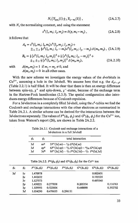
Fora 3d-electron in a completely filled 3d-shell, using the ck-tables we find the Coulomb and exchange interactions with the other electrons as summarized in Table 2A.2. l. A similar scheme can be derived for the interactions between the 3d-electrons separately. The values of Fk(<p1, <Pi) and Gk(</J1, <jJ1) for the Cu2 + ion, taken from Watson's report (26), are shown in Table 2A.2.2.
</>1 </>1
3d 1s 2s 3s 2p 3p 3d
Table 2A.2.I. Coulomb and exchange interactions of a 3d-electron in a full 3d-shell
</>1 </>1 total interaction
3d ns2 2F0 (3d,ns)- 1/5 G2(3d,ns) 3d np6 6F°(3d,np)- 2/5 G1(3d,np)- 9/s5 G8(3d,np) 3d 3d9 9F°(3d,3á)- 217 F2(3d,3á)- 217 F4(3d,3d)
Table 2A.2.2. P(</>1, <f>1) and Gk(<f>1, <f>1) for the Cu2+ ion
F°(</>1,</>1)
1.470978 1.442652 1.127073 1.450221 1.109993 1.034290
0.277038 0.523806 0.476633
F4(</>1,</>1)
0.296131
G1(</>1,</>1) G2(</>1,</>1)
0.002451 0.192235 0.489340
0.205354 0.648090
0.116763 0.392702
33
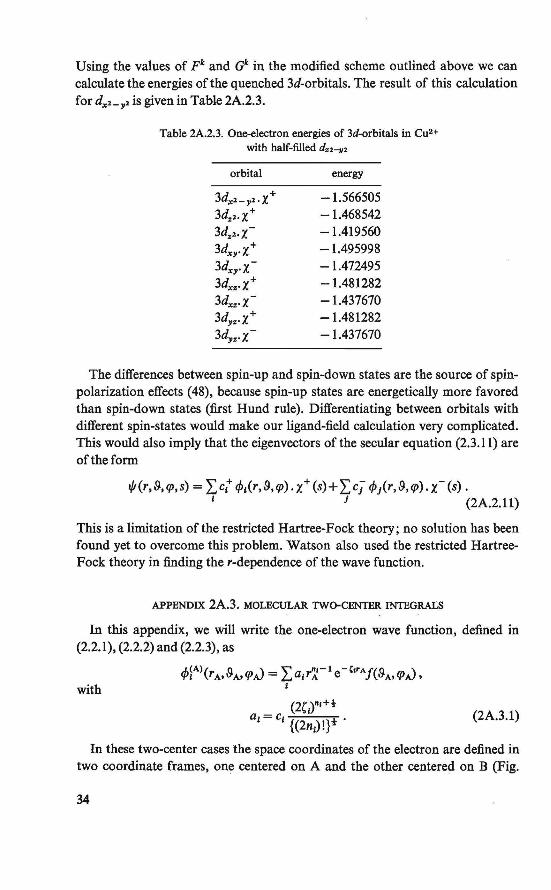
Using the values of pk and Gk in the modified scheme outlined above we can calculate the energies of the quenched 3d-orbitals. The result of this calculation for d"2_ 72 is given in Table 2A.2.3.
Table 2A.2.3. One-electron energies of 3d-orbitals in Cu2+
with half-filled d..2-y2
orbi tal energy
3d"2_,1.x+ -1.566505 3dz1·X+ -1.468542 3dz2·X- -1.419560 3dxy·X+ -1.495998
3d"".x- -1.472495 3dxz·X+ -1.481282 3d"Z'x- -1.437670 3dyz·X+ -1.481282 3dyz·X- -1.437670
The differences between spin-up and spin-down states are the source of spinpolarization effects (48), because spin-up states are energetically more favored than spin-down states (first Hund rule). Differentiating between orbitals with different spin-states would make our ligand-field calculation very complicated. This would also imply that the eigenvectors of the secular equation (2.3.11) are of the form
t/l(r,8,q>,s) = 1:Ct cf>t(r,8,q>). x+ (s)+ ~::Ci t/Jir,9,q>). x-(s). 1 i (2A.2.11)
This is a limitation of the restricted Hartree-Fock theory; no solution has been found yet to overcome this problem. Watson a]so used the restricted HartreeFock theory in finding the r-dependence of the wave function.
APPENDIX 2A.3. MOLECULAR TWO-CENTER INTEGRALS
In this appendix, we will write the one-electron wave function, defined in (2.2.1), (2.2.2) and (2.2.3), as
4'~A)(rA,8A>q>,J = L,a;r';:- 1 e-'"Af(8A,<f'~' with 1
(2()n1+t a -c --1
-..,-,- ' {(2n,)!}t .
(2A.3.1)
In these two-center cases the space coordinates of the electron are defined in two coordinate frames, one centered on A and the other centered on B (Fig.
34
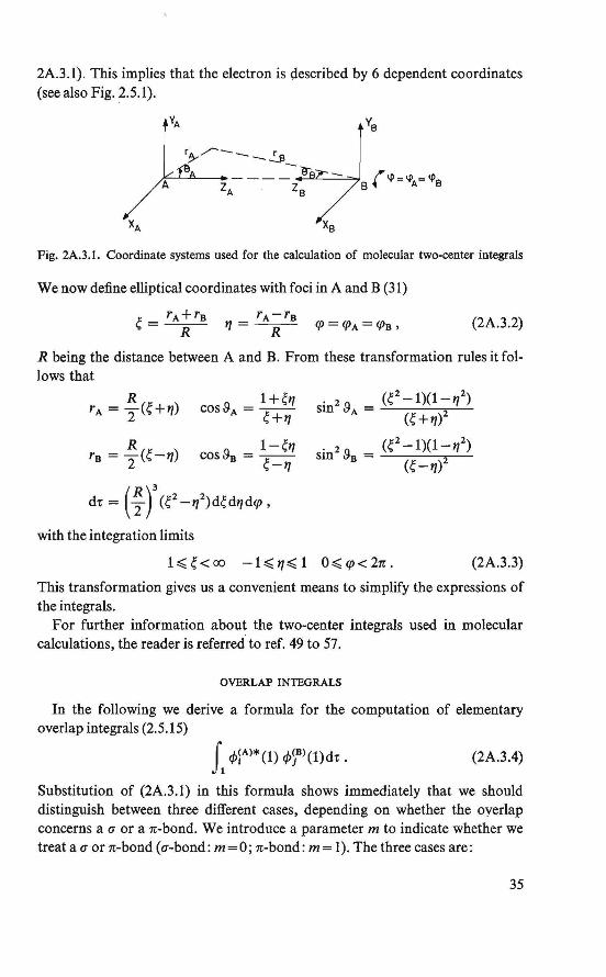
2A.3.l). This implies that the electron is çlescribed by 6 dependent coordinates (see also Fig. 2.5.1).
A
Fig. 2A.3.1. Coordinate systems used for the calculation of molecular two-center integrals
We now de:fine elliptical coordinates with foei in A and B (31)
Ç = rA +rB R <p = <fJA = <fJB, (2A.3.2)
R being the distance between A and B. From these transformation rules it follows that
R 1 +Ç17 rA = -(Ç+17) cos9A = --
2 Ç+17
R l-Ç17 rB = -(Ç-17) cos~= --
2 Ç-17
dt = ( ~ r (ç2-172)dÇd17d<p.
with the integration limits
sin 2 BA = (ÇZ-l)(l-172
)
(Ç +11)2
sin 2 9B = (ÇZ-l)(l-172
)
(Ç-17)2
1 ~ Ç < oo - 1 ~ 17 ~ 1 0 ~ <p < 2n . (2A.3.3)
This transformation gives us a convenient means to simplify the expressions of the integrals.
For further information about the two-center integrals used in molecular calculations, the reader is referred to ref. 49 to 57.
OVERLAP INTEGRALS
In the following we derive a formula for the computation of elementary overlap integrals (2.5.15)
(2A.3.4)
Substitution of (2A.3.l) in this formula shows immediately that we should distinguish between three different cases, depending on whether the overlap concerns au or an-bond. We introduce a parameter m to indicate whether we treat au or n-bond ( u-bond: m = 0; n-bond: m = 1 ). The three cases are:
35
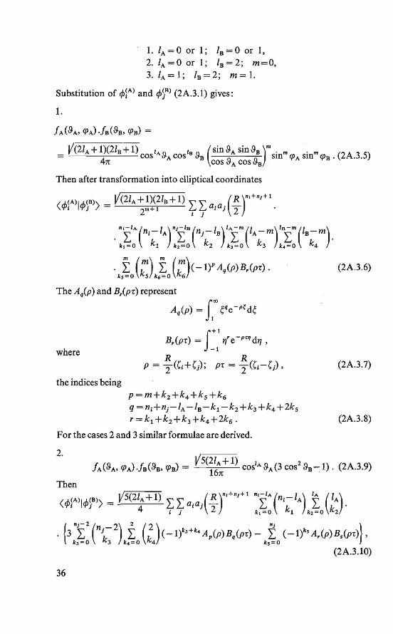
1. IA= 0 or 1; lu = 0 or 1, 2./A=Oorl; lu=2; m=O, 3. /A=l; lu=2; m=l.
Substitution of </>~A) and </>)u> (2A.3.1) gives:
1.
fA(9A, <pJ ·fu(9a, </Ju)=
_V(21A+1)(2lu+l) 1A 0 leo(sin9Asin9u)m·m ·· m (2A 3 S) -4
cos lJ' A cos ll'u 0 0 sm <p A sm </Ju . . . 1C COS l1' A COS "1l .
Then after transformation into elliptical coordinates
• k5~o (~) ko~o (~)(- l)P Aq(p)B,(pr).
The Aq(p) and B,(p•) represent
where
the indices being
Aq(p) = f~' Çqe-p~dÇ
p=m+k2 +k4 +k5 +k6
q =n1+ni-/A-lu-k1 -k2 +k3 +k4 +2k5
r=k1 +k2 +k3 +k4 +2k6 •
For the cases 2 and 3 similar formulae are derived.
2.
Then
(2A.3.6)
(2A.3.7)
(2A.3.8)
(</>~A)l</>)u» = V5(21A+l) L~>laj(~)"•+•J+l "•~A(n1 -lA) ~ (lA)· 4 i J 2 ki=O ki k1=0 k2
. {3 :~: (nik~ 2) k~J~J (-lt3+k
4 Ap(p)Bq(pt) - k~o (-l)k5 A,(p)B.(pi)},
(2A.3.10)
36
,h. d' . t e m tees bemg
3.
p = ni+n1-IA-k1 +k2 -k3 +k4 -2 q=k1+k2+k3+k4 r = n;+n1-IA-k 1 +k2 -k5
s=k1+k2+k5 •
fA(8A, <r>J.fs(Bs, <r>s) =
(2A.3.11)
V3(2ZA + 1)(218 + 1) 1A 0 10 0 (sin8A sin88 ) = cos "A cos "1l sin <f>A sin q>8 • (2A.3.12) 4n cos BA cos 88
The overlap integral is in this case f 3 x the expression (2A.3.6).
To obtain the numerical values of the integrals economically it is now important to carry out the integration quickly. It is readily shown that
and
with
q Aq(p) = Ao(P) + - Aq-1 (p)
p
e-p Ao(P) =-,
p
r B,(p;;) = B0 (p;;) + - B,_ 1 (p;;) for reven
p;;
r B,(p;;) = C(p;;) + - B,_ 1 (p;;) for r odd ,
p;;
eP'-e-P' -eP'-e-P' B0 (p;;) = and C(p;;) = ----
p;; p;;
NUCLEAR ATTRACTION INTEGRALS
The genera! expression for these integrals (2.5.8) is
Si </>~A)* (1) </>~A\1) r;} d;; .
(2A.3.13)
(2A.3.14)
(2A.3.15)
Substitution of the 8-dependent part of </>~Al leads to a general formulation of the nuclear attraction integrals. From
{g(8J} 2 = (cos2 8J1(sin2 8Jm (2A.3.16)
(2A.3.17)
37
the indices being N 1 = n1+n1-21-2m- I
r = N 1 -k1 +k2 +2k3
s= k 1 +k2 +2k4 • (2A.3.18)
The nuclear attraction integrals can be converted into these /(/, m) integrals, by carrying out the <p-integration and introducing the normalizing constants (Table 2.2.1):
«f>lA\n1, 0, O)lrä}l<J>~Al(n 1 , 0, 0)) = iJ(O, 0)
<tl>iA>(n1, 1, O)lrä"/11/>~Al(ni. 1, 0)) = tl(l, 0)
«f>lA\n 1, 1, l)lrä}l<J>lAl(n 1, 1, 1)) = tl(O, 1)
(t/>lAl(n 1 , 2, O)lrä/14>lA>(n1 , 2, 0)) = 48
51(2, 0) - 14
5 /(1, 0) + tJ(O, 0)
(tf>lAl(ni. 2, 2)1rä/ltf>fAl(n1, 2, 2)) = -ti-I(O, 2)
<4>lA>(n 1 , 2, l)lrä11 lt/>lA>(n1> 2, 1)) = ~5 1(1, 1). (2A.3.19)
COULOMB REPULSION INTEGRALS
The genera! formula for these integrals (2.5.9) is
<4>lA)(l)lf q,~B)*(2)tj>~)(2)d't'2 / <t>lA)(l)) = 2 '12
=IL 4>lAl*(l) </>lAJ(l)rïz1 </>)8 >*(2) t/>)8 '(2) d-r 1 d-r2 • (2A.3.20)
It is clear from the physical situation that this integral can be expressed as
(2A.3.21)
with U A (2) representing the potential of electron 2, caused by the charge density of electron 1, or
(2A.3.22)
As has already been mentioned in section 2.5, for the computation oftwo-center Coulomb and exchange integrals it is more convenient to decompose a quenched orbital in its constituting spherical harmonies Y1m and Yi-m (2.2.2). The final values of the integrals of quenched orbitals, are afterwards obtained from the integrals for the Yim· This becomes clear, if we use the Condon and Shortley expansion of rï2
1 (2A.2.1); see also ref. 58 and 59. The atomie orbitals to be used arethen
(2A.3.23)
Substitution of (2A.2.l) and (2A.3.23) in (2A.3.22) gives
38
"' ;. 4n * UA(2)= ;.~oµ~;.~ta1 ai 2,1,+l Y;.µ(9A2,<f'2) .
. r Yi!mA (9Al> <f'1) Yi:..m~ (9A1• <J>1) Y;.µ(9Al> <f'1)sin 9Al d9Al dq>l . J..9A J,t;01
(2A.3.24)
From (2A.2.4) it follows that U A (2) is zero unless µ=mA -m~. We define
D (Y.r +Y .r ) =îl xne-({,+{1)rA2"dx n \.i A2 \.1 A2 ·
0
which can be obtained from the recurrence relations
with
As
e-({1+{1)rA2
Eo=---((,+()rA2 •
Yim(9, q>) = ~V1 e1
m1p P1m(cos 9), 2n
(2A.3.25)
(2A.3.26)
(2A.3.27)
with P1m(cos 9) being an associate Legendre polynom.ial (60), the expression for U A (2) becomes
The space charge density J 2 </J)8 >* (2) </J)8> (2) di- equals
(2A.3.29)
Transforming the formulae (2A.3.28) and (2A.3.29) into elliptical coordinates
39
(2A.3.3) then gives the final form for the Coulomb repulsion integral as
Si''> f :: lj A(2) QB(2)( ~ r (ç2-172)dÇ d17. (2A.3.30)
This integral can be rewritten in a double quadrature sum
n n
L L A1AJ!(x1,xj) i= 1j=1
and approximated numerically (61, 62). The Gauss-Legendre formula was used, with n = 24 as a compromise between required accuracy and computation time. Tables of xk and corresponding Ak values are given by Krylov (62). This numerical integration has to be carried out between the limits - 1 < x < 1. Since the contribution to the integral is negligible for Ç > 3, at ordinary values of R ( 4-6 a. u.), the integration interval is reduced to 1 < Ç < 3, and this interval was transformed onto -1<x<1 by Ç = x+2.
EXCHANGE INTERACTION INTEGRALS
The general formula for these întegrals (2.5.10) is
<4>}A)(l)lf 4>)Bl*(2) P12</>)Bl(2)dr:21 </>}Al(l)) = 2 ri2
= JJ2 </>fAl*(l) </>)B)(l) r~21 </>}A)(2) t/>)B)*(2)dr;l dr:2. (2A.3.31)
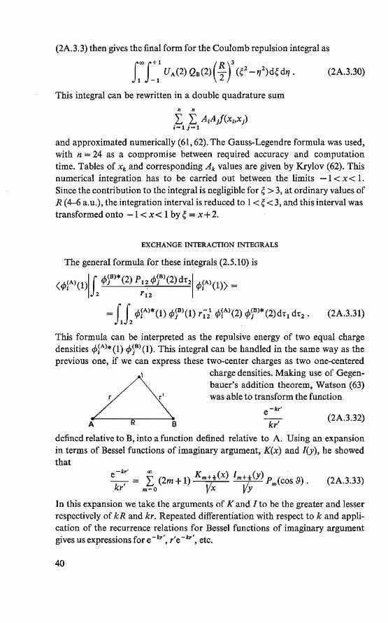
This formula can be interpreted as the repulsive energy of two equal charge densities tj>}A>*(l) t/>)8 >(1). This integral can be handled in the same way as the previous one, if we can express these two-center charges as two one-centered
A
charge densities. Making use of Gegenbauer's addition theorem, Watson (63)
r was able to transform the function
B
e -kr'
kr' (2A.3.32)
defined relative to B, into a function defined relative to A. Using an expansion in terms of Bessel functions of imaginary argument, K(x) and /(y), he showed that
e-k:' = E (2m+l) Km+t(x) lm+t(y) Pm(cos 9). kr m=O Vx VY (2A.3.33)
In this expansion we take the arguments of K and I to be the greater and lesser respectively of kR and kr. Repeated differentiation with respect tok and application of the recurrence relations for Bessel functions of imaginary argument gives us expressions for e-kr', r'e-kr', etc.
40
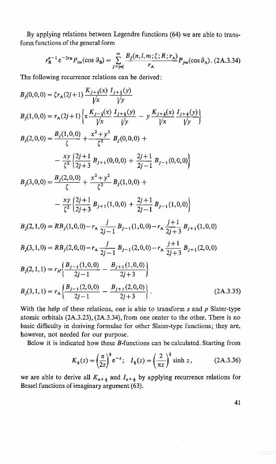
By applying relations between Legendre functions (64) we are able to transform functions of the general form
r~- l e-{•B P1m(cos 9
8) = Ï; BJ(n, l, m; (; R; r J P
1m(cos 9J. (2A.3.34)
j=JmJ rA
The following recurrence relations can be derived :
B/o,o,o) = (rA(2j+1) Kjv!<x) 11 -yy(y)
B.(l,0,0)=rA(2j+l){xK1- t(x) 11+t(Y) -yKJ+t(x) 11+t(Y)} J Vx VY Vx VY
B/2,0,0) = B1(lt,O) + x2~y2 B1(0,0,0) +
xy {2j+l 2j+l } - - 2 -.- B1+ 1 (0,0,0) + -. - B1_ 1 (0,0,0)
' 21+3 21-l
B .(3 0 0) = B1(2,0,0) xz + y2 B ·(1 0 0) J ' ' ' + (2 J ' ' +
xy {2j+l 2j+l } - ---y - .- B1+ 1 (1,0,0) + -:- B1_ 1 (1,0,0) ' 21+3 21-l
j j+l B/2, 1,0) = RB1(1,0,0)-rA -.- B1_1 (l,0,0)-rA-.- B1+ 1 (1,0,0)
21-l 21+3
j j+l Bj(3,1,0) = RBj(2,0,0)-rA-.- B1_1 (2,0,0)-rA -. - B1+ 1 (2,0,0)
21-l 21+3
B.(2 l l) = r ·{B1_ 1 (1,0,0) _ B1+ 1 (1,0,0)} J ' ' !i. 2j - 1 2j + 3
B.(3 l l) = r {B1_ 1 (2,0,0) _ B1+ 1 (2,0,0)}. J ' ' A 2j-1 2j+3
(2A.3.35)
With the help of these relations, one is able to transform s and p Slater-type atomie orbitals (2A.3.23), (2A.3.34), from one center to the other. There is no basic difficulty in deriving formulae for other Slater-type functions; they are, however, not needed for our purpose.
Below it is indicated how these B-functions can be calculated. Starting from
Kt(z) = (;zr e-•; Jt(z) = ( :z r sinh z, (2A.3.36)
we are able to derive all Kn+t and ln+t by applying recurrence relations for Bessel functions ofimaginary argument (63).
41
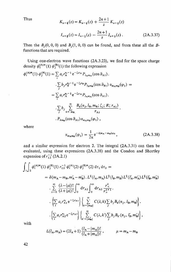
Thus
(2A.3.37)
Then the Bi(O, 0, 0) and Bi(l, 0, 0) can be found, and from these all the Bfunctions that are required.
Using one-electron wave functions (2A.3.23), we find for the space charge density </>~A)*(l) <P)Bl(l) the following expression
,i,.~A)*(l) ,i,.~B)(l) = "a.rn,-le-ç,rAp (cosO. ) 'f't 'f' J L., t A IAmA Al '
i
·Lbi Ï Bk(ni,la,ma;C;R;rA1 ).
i k= imaJ rAl
where
(2A.3.38)
and a similar expression for electron 2. The integral (2A.3.31) can then be evaluated, using these expressions (2A.3.38) and the Condon and Shortley expansion of r1z1 (2A.2.1)
IL </>~Al*(l) </>)Bl(l) r1z1 </>~A)(2) </>)Bl*(2) dr1 d1:2 =
= b(mA -m8,m~ -m~). Lt(lA,mJLt(ls, ms)L1(l~,m~ L1 (l~. m~)
"' (,1.-lµl)!J"' f"' r~ . I (,1. I I) 1 dr Al dr A2 """'ITI . .1.=0 + µ · 0 0 r>
with
42
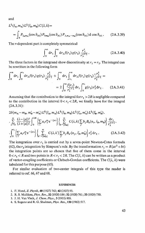
and
(2A.3.39)
The r-dependent part is completely symmetrical
(2A.3.40)
The three factors in the in te grand show discontinuity at r 1 = r 2 • The integral can be rewritten in the following form
(2A.3.41)
Assuming that the contribution to the integral for r 1 > 2R is negligible compared to the contribution in the interval 0 < r 1 < 2R, we finally have for the integral (2A.3.31):
2ö(mA -ma, m~-m;,.)Lt(lA, m~Lt(/8, m8)Lt(l~, m;,.)Lt(l~, m~).
~ (,1.-1µ1) ! f 2R {" "' -<•'•} { ~ C(À k) '\' b B ( l )} dr i • L.., (1 1 i)' 4'a;r1 e L., , 4' i k ni, e,me :::-r+I·
). = 0 11.+ µ . 0 • k=jmsl J rl
(2A.3.42)
The integration over r 1 is carried out by a seven-point Newton-Cotes formula (62), ther2 integration by Simpson's rule. By the transformation r 1 = R(at2 +bt) the integration points are so chosen that five of them come in the interval 0 < r 1 < Rand two points in R < r 1 < 2R. The C(,1., k) can be written as a product ofvector-coupling coefficients or Clebsch-Gordan coefficients. The C(,1., k) were tabulated for this purpose (65).
For sirnilar evaluation of two-center integrals of this type the reader is referred to ref. 66, 67 and 68.
REFERENCES
1. F. Hund, Z. Physik, 40 (1927) 742; 42 (1927) 93. 2. R. S. Mulliken, Phys. Rev., 32 (1928) 186; 32 (1928) 761; 33 (1929) 730. 3. J. H . Van Vleck, J. Chem. Phys., 3 (1935) 803. 4. S. Sugano and R. G. Shulman, Phys. Rev., 130 (1963) 517.
43
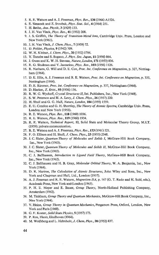
5. R. E. Watson and A. J. Freeman,Phys. Rev., 134 (1964) Al526. 6. E. Simanek and Z. Sroubek, Phys. Stat. Sol., 4 (1964) 251. 7. H. Bethe, Ann. Physik, 3 (1929) 133. 8. J. H. Van Vleck, Phys. Rev., 41 (1932) 208. 9. J. S. Griffith, The Theory of Transition-Metal !ons, Cambridge Univ. Press, London and
New York (1961). 10. J. H. Van Vleck, J. Chem. Phys., 7 (1939) 72. ll. D. Polder, Physica, 9 (1942) 709. 12. W. H. Kleiner, J. Chem.Phys., 20 (1952) 1784. 13. Y. Tanabe and S. Sugano, J. Phys. Soc. Japan, 11 (1956) 864. 14. J. Owen and K. W. H. Stevens, Nature,London, 111(1953)836. 15. R. G. ShuJman and V. Jaccarino, Phys. Rev., 103 (1956) 1126. 16. R. Nathans, G. Will and D. E. Cox, Proc. Int. Conference on Magnetism, p. 327, Notting
ham (1964). 17. D . E. Ellis, A. J. Freeman and R. E. Watson, Proc. Int. Conference on Magnetism, p. 335,
Nottingham (1964). 18. D. E. Rimmer, Proc. Int. Conference on Magnetism, p. 337, Nottingham (1964). 19. D. Harker, Z. Krist., 93 (1936) 136. 20. R. W.G. Wyekoff, Crystal Structures II, Int. Publishers, Ine., New York (1948). 21. S. W. Peterson and H.A. Levy, J. Chem. Phys., 26 (1957) 220. 22. H. ShuJI and G.G. Hall, Nature, London, 184 (1959) 1559. 23. E. U. Condon and G. H. Shortley, The Theory of Atomie Spectra, Cambridge Univ. Press,
London and New York (1953). 24. R. E. Watson, Phys. Rev., 118 (1960) 1036. 25. R. E. Watson, Phys. Rev., 119 (1960) 1934. 26. R. E. Watson, Technica/ Report, 12, Solid State and Molecular Theory Group, M.I.T.
(1959); private communieation. 27. R. E. Watson and A. J. Freeman,Phys. Rev., 123 (1961) 521. 28. F. 0. Ellison and H. Shull, J. Chem. Phys., 23 (1955) 2348. 29. J.C. Stater, Quantum Theory of Molecules and Solids 1, MeGraw-Hill Book Company,
Ine., New York (1963). 30. J.C. Slater, Quantum Theory of Molecules and So/ids Il, McGraw-Hill Book Company,
Ine., New York (1965). 31. C. J . Ballhausen, Introduction to Ligand Field Theory, McGraw-Hill Book Company,
Ine., New York (I 962). 32. C. J. Ballhausen and H. B. Gray, Molecular Orbital Theory, W. A. Benjamin, Ine., New
York(l964). 33. D. R. Hartree, The Calculation of Atomie Structures, John Wiley and Sons, Ine., New
York and Cbapman and Hall, Ltd., London (1957). 34. A. J. Freeman and R. E. Watson, Magnetism IIA, p. 167 (G.T. Rado and H. Sub!, eds.),
Academie Press, New York and London (I 965). 35. P. H . E. Meyer and E. Bauer, Group Theory, North-Holland Publishing Company,
Amsterdam (1962). 36. M. Tinkham, Group Theory and Quantum Mechanics, MeGraw-Hill Book Company, Ine.,
New York (1964). 37. V. Heine, Group Theory in Quantum Mechanics, Pergamon Press, Oxford, London, New
York and Paris (1960). 38. G. F. Koster, Solid State Physics, 5 (1957) 173. 39. P. Ros, Thesis, Eindhoven(l964). 40. M. Wolfsberg and L. Helmholz, J. Chem. Phys., 20 (1952) 837.
44
41. C. J. Ballhausenand H . B. Gray, lnorg. Chem., 1(1962)111. 42. G. W. Veltkamp and N. M. Clement, Bull. 25, Computation Center, Technologica!
University, Eindhoven (1963). 43. H. Johansen, Algol Programs /or Molecular Ca/culations, Chemistry Department, Uni
versity of Copenhagen (1965). 44. C. K. forgensen, Absorption Spectra and Chemica! Bonding in Complexes, Pergamon Press,
Oxford (1962). 45. J. Owen, Kjeller Report, 93, p. 127, Institutt for Atomenergi, Kjeller, Norway (1965). 46. W. J. O'Sullivan, W. W. Simmons and W. A. Robinson, Phys. Rev. Letters, 10 (1963) 475. 47. W. J. O'Sullivan, W. W. Simmons and W. A. Robinson, Phys. Rev., 140 (1965) Al 759. 48. P. W. Anderson, Magnetism l, p. 25 (G.T. Rado and H. Suhl, eds.), Academie Press,
New York and London (1963). 49. C. C. J. Roothaan, J. Chem. Phys., 19 (1951) 1445. 50. K . Ruedenberg, J. Chem. Phys., 19 (1951) 1459. 51. K. Ruedenberg, C. C. J. Roothaan and W. Jaunzemis, J. Chem. Phys., 24 (1956) 201. 52. C. C. J. Roothaan, J. Chem. Phys., 24 (1956) 947. 53. A.C. Wahl, P. E. Cade and C. C. J. Roothaan, J. Chem. Phys., 41 (1964) 2578. 54. A. Lofthus, Mol. Phys., 5 (1962) 105. 55. A. Lofthus, Mol. Phys., 6 (1963) 115. 56. E.A. Magnusson and C. Zauli, Proc. Phys. Soc., 78 (1961) 53. 57. E. A. Magnusson, Rev. Pure Appl. Chem., 14 (1964) 57. 58. Y. N. Chiu, J. Math. Phys., 5 (1964) 283. 59. R. A. Sack, J. Math. Phys., 5 (1964) 260. 60. Jahnke, Emde, Lösch, Tab/es of Higher Functions, B. G. Tuebner Verlagsgesellschaft,
Stuttgart (1960). 61. Z. Kopal, Numerical Analysis, Chapman and Hall, Ltd., London (1955). 62. V. 1. Krylov, Approximate Calculation of Integrals, The Macmillan Company, New York
(1962). 63. G. N. Watson, A Treatise on the Theory of Bessel Functions, Cambridge Univ. Press,
London and New York (1958). 64. E. T. Whittaker and G . N. Watson, A Course of Modern Analysis, Cambridge Univ. Press,
London and New York (1958). 65. M. Rotenberg, R. Bivins, N. Metropolis and J. K. Wooten Jr., The 3-j and 6-j Symbols,
Technology Press, M.I.T. (1959). 66. M. P. Barnett and C. A. Coulson, Phil. Trans. Roy. Soc., London, A243 (1951) 221. 67. M. P. Barnett, Methods in Computational Physics 2, p. 95 (B. Alder, S. Fernbach and
M. Rotenberg, eds.), Academie Press, New York and London (1963). 68. F. J. Corbato and A. C. Switendick, Methods in Computational Physics 2, p. 155 (B.
Alder, S. Fernbach and M. Rotenberg, eds.), Academie Press, New York and London (1963).
45
3. INTERACTIONS BETWEEN UNPAIRED ELECTRONS
IN INSULATING SOLIDS
THE MAGNETICALLY ORDERED STATE OF CuCl2 .2H20
In this chapter are described the interactions between two unpaired electrons, localized at different atomie sites in a solid . It is shown that these interactions lead to either ferromagnetic or antiferromagnetic ordering of the insulating solid. The influence of spin-orbit coupling on a system of two localized unpaired electrons is considered.
For CuCl2.2H20 the magnetically ordered structure is investigated quantitatively. The numerical values of the (exchange) interactions were obtained by using the approximated wave function of an unpaired electron localized at a Cu2+ site (chapter 2) in the mechanism described.
3.1. INTRODUCTION
The first explanation of exchange interactions was given by Heisenberg (1). He showed that the Coulomb repulsion between two electrons leads to an exchange interaction which couples the two electron spins parallel to each other. Dirac (2) proved that the exchange interaction for two electrons with spins S 1 and S2 can be expressed in the formula
-J(-t+2S1 .S2),
with J the (direct) exchange integral.
J = f f <Pi(l) <Pil) r;z1 <Pi(2) <Pi2) d•1 dr2
(3.1.1)
(3.1.2)
Since in practice the integral (see also 2.5.10) is always positive, the interaction always favors a parallel alignment of the electron spins. Van Vleck (3) first used the expression (3.1.1) as a basis for the theory of ferromagnetism.
The approximation of the Heisenberg-Dirac-Van Vleck hamiltonian
(3.1.3)
has proven to be very useful. However, the occurrence of antiferromagnetism, i.e. an antiparallel alignment of the electron spins, cannot be explained by this model. Neither is it in first instance clear why there exist interactions between unpaired electrons which are far apart, for instance in diluted salts. Kramers (4) was the first to introduce the idea of superexchange, i.e. how the ordering interaction works over long distances. His idea was that two unpaired electrons localized at atom sites A and B on opposite sides of a diamagnetic atom induce this diamagnetic atom in such a way that the antiparallel alignment of the electron spins at A and B is favored over the parallel alignment. After the
46
introduction of this conception, many specific realizations based on Kramers' superexchange idea were proposed (5, 6). The latter have been gradually modified, eventually resuiting in the model proposed by Anderson (7, 8, 9, 10).
Anderson, by using perturbation theory, showed that besides the exchange interaction (3.1.1) between two electrons, an overlap effect between two electrons, localized at different atoms, favors the antiparallel alignment of the eiectron spins. He derived that the interaction between two Iocalized electrons with spins S 1 and S 2 can be written in the form
(3.1.4)
with J representing the direct exchange and 2b2/V the superexchange. The quantity bis the matrix element of the self-consistent Hartree-Fock hamiltonian of the crystal connecting the two one-electron states for which the interaction is considered. U denotes the energy difference of the electron in the state Iocalized at A, with the one in which the electron is transferred to a localized state at B.
According to Anderson, the unpaired eiectron is transferred from A to B by the amount (b/ V)2
• He shows that this effect is microscopically the most important origin of antiferromagnetism, by assuming that the only important admixed state is the state in which the transferred spin is antiparallel to the electron spin(s) localized at B. This mechanism proposed is roughly analogous to the Heitler-London scheme of chemica! bonding (11).
In the next section we shall show that the Coulomb repulsion between two electrons can also favor the spin-antiparallel state over the spin-parallel state. According to this theory it follows that superexchange as well as direct exchange originate from the Coulomb repulsion. The expression derived for the superexchange bas the practical advantage that the interactioncan be calculated, which provides the possibility of a quantitative test of the model.
We are now confronted with two exchange mechanisms: the transfer effect and the one due to the Coulomb repulsion. However, we believe that in strongly diluted magnetic substances, Iike CuCl2 .2H2 0 , the transfer effect is much smaller than the other, and only the Coulomb repulsion gives rise to exchange interactions. This expectation is supported by the calculated numerical values of the exchange interactions in CuC12 .2H20, owing to the Coulomb repulsion. Unfortunately, the transfer effect cannot be calculated numerically, because of the extremely complicated form of the matrix element b. Anderson, however, shows that the term 2b2
/ U in the case of KNiF 3 is of the same order of magnitude as the experimentally determined values of the superexchange interaction.
Against the transfer effect the following objections can be raised : 1. It is not clear, why the mechanism leads to a lowering of only the spin
antipara!lel state (electron transfer to empty orbitals). 2. The electron transfer to empty orbitals at diamagnetic ions intervening the
magnetic ions, should be considered.
47
Thus, the conclusion is that the transfer effect is very complex, and one cannot decide upon this mechanism before it has been calculated.
3.2. MECHANISM OF ISOTROPIC EXCHANGE INTERACTIONS IN INSULATORS
It is generally accepted that in insulators localized one-electron wave functions can be considered as eigenfunctions of the self-consistent Hartree-Fock hamiltonian of the crystal. We use the following notation for a function localized at A:
p(A) (1) • (3.2.1)
The present section deals with the interaction between two unpaired electrons localized at different magnetic ion sites. To find the interaction between the two electrons, we consider this two-electron system. The total wave function of the two-electron system must be antisymmetric. We assume the total wave function to be a product of a space and spin-dependent part. Then either the space or the spin-dependent part is antisymmetric. The former case corresponds to the parallel alignment of the spins, the Jatter to the antiparallel alignment. As the electrostatic interactions are by far the strongest, we ignore other interactions. In the case of the symmetrie spin-dependent part, the spin functions are equal, the arising extra (quantum mechanica!) coupling energy of two parallel spins is the time-honored Heisenberg exchange.
In the following we consider the system of two localized unpaired electrons. h follows that the Coulomb repulsion gives an energy lowering of the spinantiparallel state as well as of the spin-parallel state. From the numerical calculation of this interaction between neighboring unpaired electrons in CuCl2 .2H20, we conclude that the energy lowering of the spin-antiparallel state due to the Coulomb repulsion agrees numerically with the values of the superexchange interactions in CuCl2 .2H2 0.
In this formalism the Coulomb repulsion is the microscopie origin of ferromagnetism and antiferromagnetism. The type of magnetic ordering of a substance depends on the relative values of the direct exchange and the superexchange interactions. The spin hamiltonian (12) resulting from the theory is a strong argument to apply the Heisenberg-Dirac-Van Vleck hamiltonian also for describing antiferromagnetic materials (3.1.3).
For simplicity, it is supposed that each magnetic ion has only one unpaired electron, and that the wave function of an unpaired electron can be written as
(3.2.2)
a product of the space-dependent part cjJ<A>(l) and the spin-dependent part x<A>(l). The perturbation hamiltonian of the two-electron system is
(3.2.3)
48
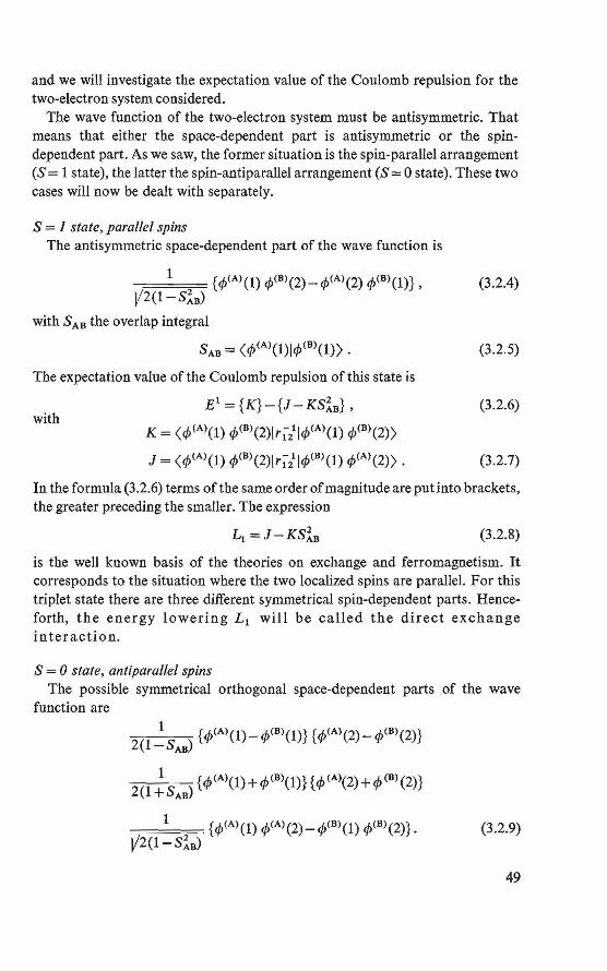
and we will investigate the expectation value of the Coulomb repulsion for the two-electron system considered.
The wave function of the two-electron system must be antisymmetric. That means that either the space-dependent part is antisymmetric or the spindependent part. As we saw, the former situation is the spin-parallel arrangement (S= 1 state), the latter the spin-antiparal!el arrangement (S= 0 state). These two cases will now be dealt with separately.
S = 1 state, parallel spins The antisymmetric space-dependent part of the wave function is
1 2 {<f/Al(l) </J(B)(2)-<f/A)(2) </J(B\1)}' V2(1-SAB)
with SAB the overlap integral
SAB = <<P(A)(l)l</J(B)(l)).
The expectation value of the Coulomb repuls ion of this state is
with E1 = {K}-{J-KS!8 },
K = <<P(A)(l) </J(B)(2)1rïll</J(A)(l) </J(B)(2))
J = (</J(A)(l) </J(B)(2)lrïll</J(B)(l) </J(A)(2)) ·
(3.2.4)
(3.2.5)
(3.2.6)
(3.2.7)
In the formula (3.2.6) terms of the same order of magnitude are put in to brackets, the greater preceding the smaller. The expression
(3.2.8)
is the well known basis of the theories on exchange and ferromagnetism. It corresponds to the situation where the two localized spins are parallel. For this triplet state there are three different symmetrical spin-dependent parts. Henceforth, the energy lowering L 1 will be called the direct exchange interaction.
S = 0 state, antiparallel spins The possible symmetrical orthogonal space-dependent parts of the wave
function are
1 {</J(A)(l)-</J(B)(l)} {</J(A)(2)-</J(B)(2)} 2(1-SAB)
1 { </J(A)(l)+ </J(B)(l)}{ </J (A)(2)+ </J (B) (2)} 2(1 +SAB)
1 . _ {</J(A)(l) </J(A)(2)-</J(B)(l) </J(B)(2)}. V2(1-S!B)
(3.2.9)
49
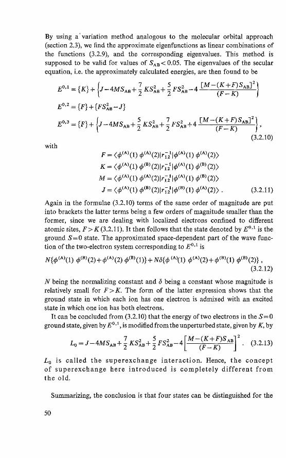
By using a' variation method analogous to the molecular orbital approach (section 2.3), we find the approximate eigenfunctions as linear combinations of the functions (3.2.9), and the corresponding eigenvalues. This metbod is supposed to be valid for values of S AB< 0.05. The eigenvalues of the secular equation, i.e. the approximately calculated energies, are then found to be
with
E0 •1 ={K}+{J-4MS +2Ks2 +~Fs2 -4 [M-(K+F)sABJ2
} AB 2 AB 2 AB (F-K)
E 0•2 = {F}+{FS,!B-J}
0 3 { } { 5 2 7 2 [ M - ( K + F) s AB] 2
} E' = F + J-4MSAB+Ï:KSAB+Ï:FSAB+4 (F-K) ,
F = (</>(A)(l) ct><Al(2)1rïllc/>(A)(l) c/>(A)(2))
K = (c/>(A)(l) <J><B>(2)1rïllc/>(A)(l) ct><B>(2))
M = (<p<Al(l) c/>(A)(2)1rïllc/><A\1) c/>(B)(2))
J = (c/>(A)(l) </>(B)(2)1rïllc/>(B)(l) </>(A)(2)) ·
(3.2.10)
(3.2.11)
Again in the formulae (3.2.10) terms of the same order of magnitude are put into brackets the Jatter terms being a few orders of magnitude smaller than the former, since we are dealing with locaJized electrons confined to different atomie sites, F > K (3.2.11). It then follows that the state denoted by E 0
•1 is the
ground S=O state. The approximated space-dependent part of the wave function of the two-electron system corresponding to E 0
•1 is
N{</>(A)(l) </>(B)(2)+</><A\2) c/>(B)(l)}+Nö{</>(A)(l) </>(A)(2)+</>(B)(l) </>(B)(2)} '
(3.2.12)
N being the normalizing constant and ö being a constant whose magnitude is relatively small for F >K. The form of the Jatter expression shows that the ground state in which each ion bas one electron is admixed with an excited state in which one ion bas both electrons.
It can be concluded from (3.2.10) that the energy of two electrons in the S = 0 ground state, given by E 0
•1
, is modified from the unperturbed state, given by K, by
7 2 5 2 [M-(K+F)SAB]2
L0 =J-4MSAB+2KSAB+ÏFSAB-4 (F-K) . (3.2.13)
L 0 is called the superexchange interaction. Hence, the concept of superexchange here introduced is compJetely different from the old.
Summarizing, the conclusion is that four states can be distinguished for the
50
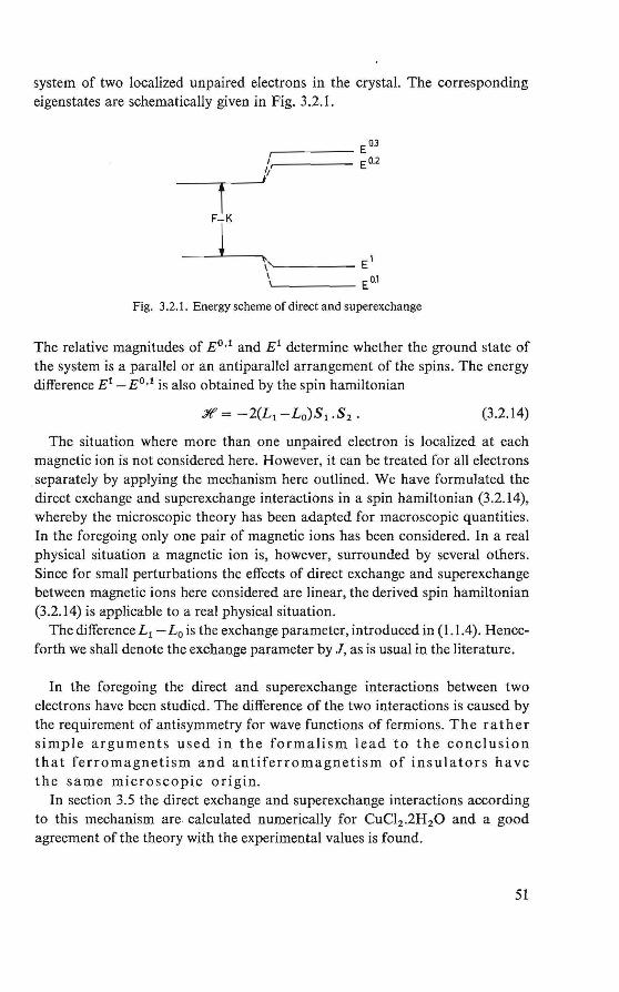
system of two localized unpaired electrons in the crystal. The corresponding eigenstates are schematically given in Fig. 3.2.1.
~'-----El 1 Eo.1
Fig. 3.2.1. Energy scheme of direct and superexchange
The relative magnitudes of E 0•1 and E 1 determine whether the ground state of
the system is a parallel or an anti parallel arrangement of the spins. The energy difference E1 -E0
•1 is also obtained by the spin hamiltonian
(3.2.14)
The situation where more than one unpaired electron is localized at each magnetic ion is not considered here. However, it can be treated for all electrons separately by applying the mechanism here outlined. We have formulated the direct exchange and superexchange interactions in a spin hamiltonian (3.2.14), whereby the microscopie theory has been adapted for macroscopie quantities. In the foregoing only one pair of magnetic ions has been considered. In a real physical situation a magnetic ion is, however, surrounded by several others. Since for small perturbations the effects of direct exchange and superexchange between magnetic ions here considered are linear, the derived spin hamiltonian (3.2.14) is applicable to a real physical situation.
The difference L1 - L 0 is the exchange parameter, introduced in ( l .1.4). Henceforth we shall denote the exchange parameter by J, as is usual in the literature.
In the foregoing the direct and superexchange interactions between two electrons have been studied. The difference of the two interactions is caused by the requirement of antisymmetry for wave functions of fermions. The ra ther simple arguments used in the formalism lead to the conclusion that ferromagnetism and antiferromagnetism of insulators have the same microscopie origin.
In section 3.5 the direct exchange and superexchange interactions according to this mechanism are calculated numerically for CuCl2 .2H20 and a good agreement of the theory with the experimental values is found.
51
3.3. THE INFLUENCE OF SPIN-ORBIT COUPLING
In this section we study the infiuence of spin-orbit coupling on a system of two localized electrons.
The one-electron hamiltonian, representing the spin-orbit coupling is (13, 14)
::lf = !S. (Vd// x p) , (3.3.1)
d/t being the potential, p the momentum and S the spin of the electron. The hamiltonian can be rewritten in the conventional way
::lf = 2A(l) . S(l) = A + (1) s-(1) + A- (1) s+(l)+2Az(l) Sz(l), with
(3.3.2)
From the variation method in 3.2 it followed (3.2.12) that for antipara!lel spins at atom sites A and B, the one-electron wave function mainly localized at A is given by
(3.3.3)
x+ and x- denoting the spin-up and spin-down states respectively. In the state (3.3.3) the spin-orbit coupling causes an energy change
L1E = 4ó(<f>(B)(J)IA+ (l)l</>(A)(l)), (3.3.4)
For two localized electrons with parallel spins this energy shift does not appear, because in the S = 1stateö=0 (3.2.4).
Moriya (14, 15) arrived at a similar expression using Anderson's exchange mechanism. He pointed out that the energy shift could lead to a canting of the electron spins from the exact anti parallel direction, if such magnetic structure is allowed by the symmetry of the crystal. He, too, showed (16, 17) that also inequivalent environments of transition metal ions by Iigands may lead to a canting of antiferromagnetically ordered spins. In this case the easy axes of the anisotropy energy on two magnetic ions are not parallel, which may result in a canting of the electron spins. Fora fuller treatment of this effect and also for the description of macroscopie properties of antiferromagnetics with a weak ferromagnetism, the reader is referred to ref. 17.
3.4. STUDIES OF THE MAGNETIC STATE OF CuC12.2H20
Experimental work Copper chloride is probably the antiferromagnetic substance most in
vestigated experimentally. Most of the early work was done at the Kamerlingh Onnes Laboratory in Leiden. Gorter (18) reviews the most important results.
52
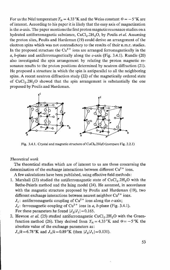
For us the Néel temperature TN = 4.33 °K and the Weiss constant e = -5 °K are of interest. According to his paper it is likely that the easy axis of magnetization is the a-axis. The paper mentions the first proton magnetic resonance studies on a hydrated antiferromagnetic substance, CuCl2 .2H20, by Poulis et al. Assuming the proton sites, Poulis and Hardeman (19) could derive an arrangement of the electron spins which was not contradictory to the results oftheir n.m.r. studies. In the proposed structure the Cu2 + ions are arranged ferromagnetically in the a, b-plane and antiferromagnetically along the c-axis (Fig. 3.4.1 ). Rundle (20) also investigated the spin arrangement by relating the proton magnetic resonance results to the proton positions determined by neutron diffraction (21). He proposed a structure in which the spin is antiparallel to all the neighboring spins. A recent neutron diffraction study (22) of the magnetically ordered state of CuC12 .2H20 showed that the spin arrangement is substantially the one proposed by Poulis and Hardeman.
c c
b
Fig. 3.4.1. Crystal and magnetic structure of CuCl2.2H20 (compare Fig. 2.2.1)
Theoretica/ work The theoretica! studies which are of interest to us are those concerning the
determination of the exchange interactions between different Cu2 + ions. A few calculations have been published, using effective field methods:
1. Marshall (23) studied the antiferromagnetic state of CuC12 .2H20 with the Bethe-Peierls method and the Ising model (24). He assmned, in accordance with the magnetic structure proposed by Poulis and Hardeman (19), two different exchange interactions between nearest neighbor eu2 + ions. J 1 : antiferromagnetic coupling of Cu2 + ions along the c-axis; J2 : ferromagnetic coupling of Cu2 + ions in a, b-plane (Fig. 3.4.1). For these parameters he found IJ2/J1 1 =0.165.
2. Hewson et al. (25) studied antiferromagnetic CuC12 .2H20 with the Greenfunction method (26). They derived from TN = 4.33°K and E>= -5°K the absolute value of the exchange parameters as: Jifk=6.78°K and J2 /k=0.89°K (then IJ2/Ji1=0.131).
53
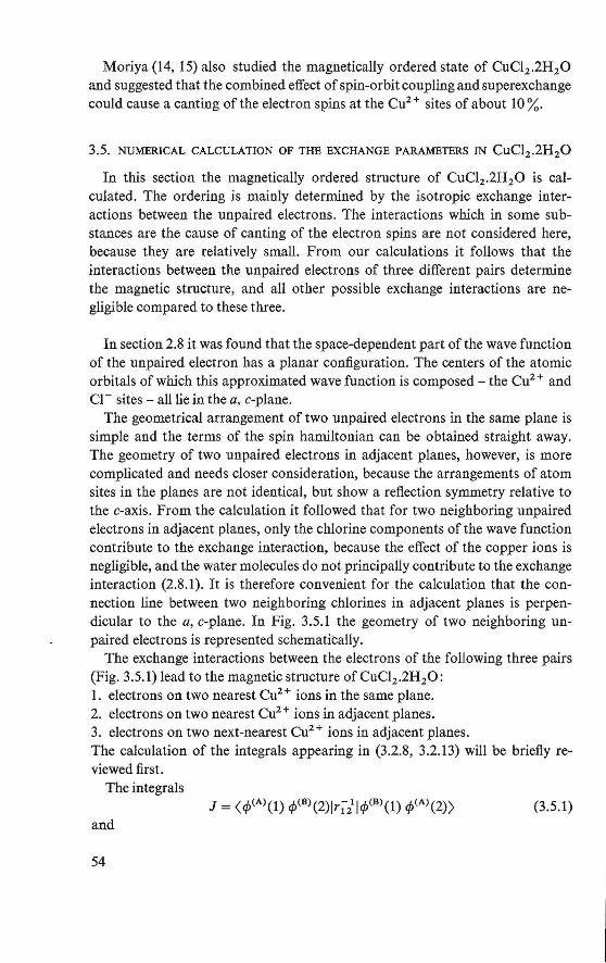
Moriya (14, 15) also studied the magnetically ordered state of CuCl2 .2H20 and suggested that the combined effect of spin-orbit coupling and superexchange could cause a canting of the eiectron spins at the Cu2 + sites of about 10 %.
3.5. NUMERICAL CALCULATION OF THE EXCHANGE PARAMETERS IN CuCl2 .2H20
In this section the magnetically ordered structure of CuCl2 .2H2 0 is calculated. The ordering is mainly determined by the isotropic exchange interactions between the unpaired electrons. The interactions which in some substances are the cause of canting of the electron spins are not considered here, because they are relatively small. From our calculations it follows that the interactions between the unpaired electrons of three different pairs determine the magnetic structure, and all other possible exchange interactions are negligible compared to these three.
In section 2.8 it was found that the space-dependent part of the wave function of the unpaired electron has a planar configuration. The centers of the atomie orbitals of which this approximated wave function is composed - the Cuz+ and Cl - sites - all lie in the a, c-plane.
The geometrical arrangement of two unpaired electrons in the same plane is simple and the terms of the spin hamiltonian can be obtained straight away. The geometry of two unpaired electrons in adjacent planes, however, is more complicated and needs closer consideration, because the arrangernents of atom sites in the planes are not identical, but show a refiection symrnetry relative to the c-axis. From the calculation it followed that for two neighboring unpaired electrons in adjacent planes, only the chlorine components of the wave function contribute to the exchange interaction, because the effect of the copper ions is negligible, and the water molecules do not principally contribute to the exchange interaction (2.8.1). It is therefore convenient for the calculation that the connection line between two neighboring chlorines in adjacent planes is perpendicular to the a, c-plane. In Fig. 3.5. l the geometry of two neighboring unpaired electrons is represented schematically.
The exchange interactions between the electrons of the following three pairs (Fig. 3.5.1) lead to the magnetic structure of CuCl2 .2H20: 1. electrons on two nearest Cu2 + ions in the same plane. 2. electrons on two nearest Cu2 + ions in adjacent planes. 3. eiectrons on two next-nearest eu2 + ions in adjacent planes. The calculation of the integrals appearing in (3.2.8, 3.2.13) will be briefiy reviewed first.
The integrals (3.5.1)
and
54
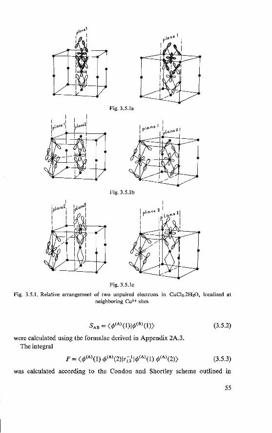
Fig. 3.5.Ja
Fig. 3.5.Jb
Fig. 3.5.lc
Fig. 3.5.1. Relative arrangement of two unpaired electrons in CuCl2.2H20, localized at neighboring Cu2+ sites
(3.5.2)
were calculated using the formulae derived in Appendix 2A.3. The integral
(3.5.3)
was calculated according to the Condon and Shortley scheme outlined in
55
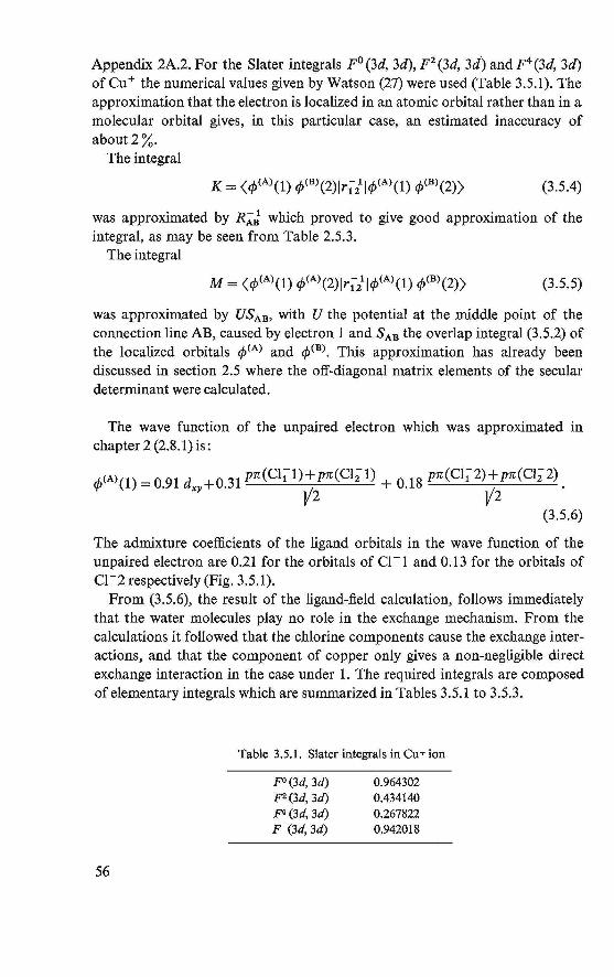
Appendix 2A.2. For the Slater integrals F 0 (3d, 3d), F 2 (3d, 3d) and F4 (3d, 3d) of cu+ the numerical values given by Watson (27) were used (Table 3.5.1). The approximation that the electron is localized in an atomie orbital rather than in a molecular orbital gives, in this particular case, an estimated inaccuracy of about2%.
The integral
(3.5.4)
was approximated by RAi which proved to give good approximation of the integral, as may be seen from Table 2.5.3.
The integral
(3.5.5)
was approximated by USAa. with U the potential at the middle point of the connection line AB, caused by electron 1 and SAB the overlap integral (3.5.2) of the localized orbitals <jJ<A> and <jJ<B>. This approximation has already been discussed in section 2.5 where the off-diagonal matrix elements of the secular determinant were calculated.
The wave function of the unpaired electron which was approximated in chapter 2 (2.8.1) is:
<P(A)(l) = 0.91 dxy+0.31 pn(Cl!l);;n(CI;l) + 0.18 pn(Cl12)V2pn(Cl22).
(3.5.6)
The admixture coefficients of the ligand orbitals in the wave function of the unpaired electron are 0.21 for the orbitals of Cl -1 and 0.13 for the orbitals of c1-2 respectively (Fig. 3.5.1).
From (3.5.6), the result of the ligand-field calculation, follows immediately that the water molecules play no role in the exchange mechanism. From the calculations it followed that the chlorine components cause the exchange interactions, and that the component of copper only gives a non-negligible direct exchange interaction in the case under 1. The required integrals are composed of elementary integrals which are summarized in Tables 3.5.1 to 3.5.3.
56
Table 3.5.1. Stater integrals in Cu+ ion
po(3d, 3d) F2(3d, 3d) F4 (3d, 3d) F (3d, 3d)
0.964302 0.434140 0.267822 0.942018
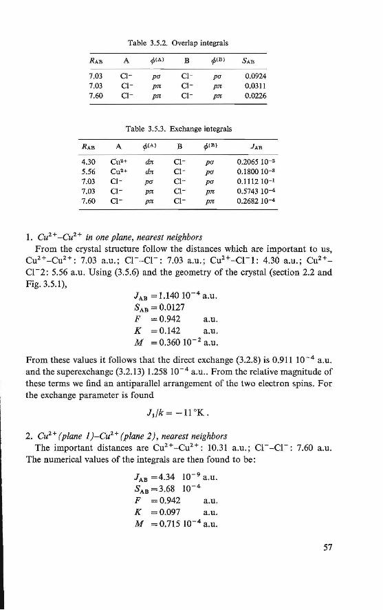
Table 3.5.2. Overlap integrals
RAB A </>(A) B <f><B) SAB
7.03 Cl- pa Cl- pa 0.0924 7.03 Cl- pn Cl- pn 0.0311 7.60 Cl- pn Cl- pn 0.0226
Table 3.5.3. Exchange integrals
RAB A </>(A) B <f><B) JAB
4.30 Cu2+ dn Cl- pa 0.2065 10-2
5.56 Cu2+ dn c1- pa 0.1800 10-s 7.03 Cl- pa c1- pa 0.1112 10-1
7.03 Cl- pn c1- pn 0.5743 10-4 7.60 Cl- pn Cl- pn 0.268210-4
1. Cu2 + -Cu2 + in one plane, nearest neighbors From the crystal structure follow the distances which are important to us,
eu2 +-cu2 +: 7.03 a.u.; c1--c1-: 7.03 a.u.; Cu2+-c1-1: 4.30 a.u.; Cu2 +c1-2: 5.56 a.u . Using (3.5.6) and the geometry of the crystal (section 2.2 and Fig. 3.5.1),
JAB = 1.140 10- 4 a.u. SAB = 0.0127 F = 0.942 a.u. K = 0.142 a.u . M = 0.360 10- 2 a.u.
From these values it follows that the direct exchange (3.2.8) is 0.911 10-4 a .u. and the superexchange (3.2.13) 1.258 10- 4 a.u .. From the relative magnitude of these terms we find an antiparallel arrangement of the two electron spins. For the exchange parameter is found
Jifk=-I1 °K.
2. Cu2 + (plane J)-Cu2 + (plane 2), nearest neighbors The important distances are Cu2 + - Cu2+: 10.31 a .u.; Cl--Cl-: 7.60 a.u.
The numerical values of the integrals are then found to be:
JAB =4.34 10- 9 a.u . SAB=3.68 10- 4
F = 0.942 a.u. K = 0.097 a.u. M = 0.715 10- 4 a.u.
57
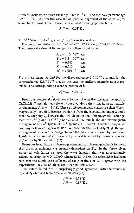
From this follows the direct exchange -8.8 10- 9 a.u. and for the superexchange 122.8 10- 9 a.u. Also in this case the antiparallel alignment of the spins is preferred to the parallel one. Hence the calculated exchange parameter is
J;/k = -0.04°K.
3. Cu2 + (plane J)-Cu2+ (plane 2), next-nearest neighbors The important distances are Cu2 +-cu2 +: 12.48 a.u.; c1--c1-: 7.60 a.u.
The numerical values of the integrals are then found to be:
lAB =4.10 10-s a.u. SAB =6.24 10- 4 a.u. F = 0.942 a.u. K = 0.080 a.u. M = 1.001 10- 4 a.u.
From these terms we find for the direct exchange 9.8 10- 9 a.u. and for the superexchange 525.7 10- 9 a.u. In this case the antiferromagnetic state is preferred. The corresponding exchange parameter is
l~/k = -O.l6°K.
From our numerical calculation it follows that in first instance the spins in CuC12 .2H20 are relatively strongly coupled along the c-axis in an antiparallel arrangement: lifk = -11 °K. These antiferromagnetic chains are then "ferromagnetically" coupled, because we derive from the calculations under 2 and 3 that the coupling 12 between the two chains in the "ferromagnetic" arrangement of Cu2 +(plane 1)-Cu2 +(plane 2) is 0.60°K and in the antiferromagnetic arrangement of Cu2 +(plane 1)-Cu2 +(plane 2): -0.60 °K. The "ferromagnetic" coupling is favored: 12/k = 0.60 °K. We conclude that for CuCl2 .2H20 the spin arrangement is the antiferromagnetic one that has been proposed by Poulis and Hardeman (19), and which has recently been determined by means of neutron diffraction by Shirane et al. (22).
From our formulation offerromagnetism and antiferromagnetism it followed that the superexchange was strongly dependent on SAB· In the above given numerical calculation we used the wave function that was approximately calculated using the MO-LCAO scheme (2.8.1, 3.5.6). In section 2.8 it has been said that the admixture coefficient of the p-orbitals of Cl -2 agrees with the experimental results obtained for other materials (28).
The values found are in surprisingly good agreement with the values of 11 and 12 obtained from experimental data (25)
lifk = - 6.78 °K 12 /k = 0.89°K.
58
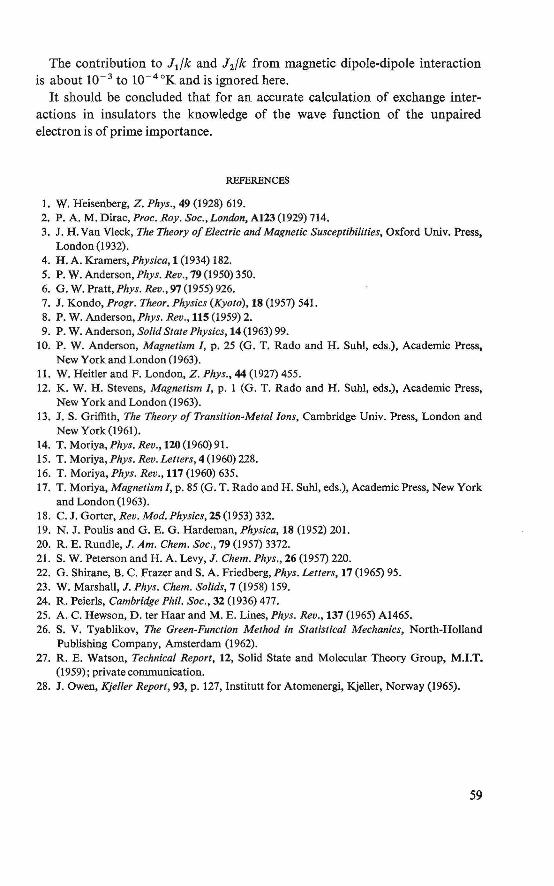
The contribution to Jif k and 12 /k from magnetic dipole-dipole interaction is about 10- 3 to 10-4 °K and is ignored here.
It should be concluded that for an accurate calculation of exchange interactions in insulators the knowledge of the wave function of the unpaired electron is of prime importance.
REFERENCES
1. W. Heisenberg, Z. Phys., 49 (1928) 619. 2. P. A. M. Dirac, Proc. Roy. Soc., London, A123 (1929) 714. 3. J. H. Van Vleck, The Theory of Electric and Magnetic Susceptibilities, Oxferd Univ. Press,
Londen (1932). 4. H.A. Kramers, Physica, 1 (1934) 182. 5. P. W. Anderson, Phys. Rev., 19 (1950) 350. 6. G. W. Pratt, Phys. Rev., 97 (1955) 926. 7. J. Kondo, Progr. Theor. Physics (Kyoto), 18 (1957) 541. 8. P. W. Anderson, Phys. Rev., 115 (1959) 2. 9. P. W. Anderson, Solid State Physics, 14 (1963) 99.
10. P. W. Anderson, Magnetism l, p. 25 (G.T. Rado and H. Suhl, eds.), Academie Press, New York and London (1963).
11. W. Heitler and F. London, Z. Phys., 44 (1927) 455. 12. K. W. H. Stevens, Magnetism I, p. l (G.T. Rado and H. Suhl, eds.), Academie Press,
New York and London (1963). 13. J . S. Griffith, The Theory of Transition-Meta/ Ions, Cambridge Univ. Press, London and
New York (1961). 14. T. Meriya,Phys. Rev., 120(1960)91. 15. T. Moriya,Phys. Rev.Letters,4(1960)228. 16. T. Moriya, Phys. Rev., 117 (1960) 635. 17. T. Meriya, Magnetism l, p. 85 (G.T. Rado and H. Suhl, eds.), Academie Press, New York
and Londen (1963). 18. C. J. Gorter, Rev. Mod. Physics, 25 (1953) 332. 19. N. J. Poulis and G. E.G. Hardeman, Physica, 18 (1952) 201. 20. R. E. Rundle, J. Am. Chem. Soc., 79 (1957) 3372. 21. S. W. Peterson and H.A. Levy, J. Chem. Phys., 26 (1957) 220. 22. G. Shirane, B. C. Frazer and S. A. Friedberg, Phys. Letters, 17 (1965) 95. 23. W. Marshall, J. Phys. Chem. Solids, 7 (1958) 159. 24. R. Peierls, Cambridge Phil. Soc" 32 (1936) 477. 25. A.C. Hewson, D. ter Haar and M. E. Lines, Phys. Rev" 137 (1965) Al465. 26. S. V. Tyablikov, The Green-Function Method in Statistica! Mechanics, North-Helland
Publishing Company, Amsterdam (1962). 27. R. E. Watson, Technica/ Report, 12, Solid State and Molecular Theory Group, M.I.T.
(1959); private cemmunication. 28. J. Owen, Kjeller Report, 93, p. 127, Institutt for Atomenergi, Kjeller, Norway (1965).
59
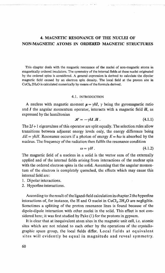
4. MAGNETIC RESONANCE OF THE NUCLEI OF
NON-MAGNETIC ATOMS IN ORDERED MAGNETIC STRUCTURES
This chapter deals with the magnetic resonance of the nuclei of non-magnetic atoms in magneticaliy ordered insulators. The symmetry of the internal fields at these nuclei originated by the ordered spins is considered. A genera! expression is derived to calculate the dipolar magnetic field caused by an electron spin density. The local field at the proton site in CuC12.2H20 is calculated numerically by means of the formula derived.
4.1. INTRODUCTION
A nucleus with magnetic momentµ= yhl, y being the gyromagnetic ratio and I the angular momentum operator, interacts with a magnetic field H, as expressed by the hamiltonian
Yf= -yhl.H. (4.1.1)
The 21+1 eigenvalues ofthis operator are split equally. The selection rules allow transitions between adjacent energy levels only, the energy difference being LJE = yhH. Resonance occurs if a photon of energy E = hw is absorbed by the nucleus. The frequency of the radiation then fulfils the resonance condition
w = yH. (4.1.2)
The magnetic field of a nucleus in a solid is the vector sum of the externally applied and of the internal fields arising from interactions of the nuclear spin with the ordered electron spins in the solid. Assuming that the angular momentum of the electron is completely quenched, the effects which may cause this internal field are: 1. Dipolar interactions. 2. Hyperfine interactions.
According to the result of the ligand-field calculation in chapter 2 the hyperfine interactions of, for instance, the Hand 0 nuclei in CuCl2 .2H20 are negligible. Sometimes a splitting of the proton resonance Iines is found because of the dipole-dipole interaction with other nuclei in the solid. This effect is not considered here; it was first studied by Pake (1) for the protons in gypsum.
lt is clear that at inequivalent atom sites in the magnetic unit cell, i.e. atomie sites which are not related to each other by the operations of the crystallographic space group, the local fields differ. Local fields at equivalent sites will evidently be equal in magnitude and reveal symmetry.
60
A general treatment of nuclear magnetic resonance in these solids has recently been given by Jaccarino (2).
4.2. SYMMETRY OF THE LOCAL FIELDS
The symmetry of magnetic fields at positions in the chemica! unit ceII, related to each other by operations of the space group, is of considerable importance as regards the study of magnetic structures. The symmetry of the local fields in these structures has been studied by Riedel and Spence (3). They apply the theory of Shubnikov groups or magnetic space groups for their purpose. Riedel deals extensively with this matter in his thesis (4).
After indicating the genera! themes of magnetic space group theory, we shall summarize the ideas of Riedel and Spence. Then we shall extend the work described by Riedel ( 4) by deriving which of the magnetic point groups correspond to a certain symm.etry of these local fields.
An angular magnetic moment is caused by a circular current and is thus transformed as an axial vector, and changes sign under time inversion. These transformation rules also hold for the magnetic moment caused by the spin moment. A crystal is regarded as a statie arrangement of atoms, which is invariant under the operations of the space group. Deviating from the definition of a crystal, we define a magnetic crystal as a statie arrangement of atoms where magnetic moments of equal magnitude are attached to equivalent atoms. A magnetic space group is defined as a group of elements, which leaves a statie arrangement of magnetic moments invariant. We here introduce the product group G of the space group and the group consisting of the identity E and the time inversion operation E'. From the de:finition it then follows that a magnetic crystal is not invariant under the operations of such a product group: a magnetic space group must not contain the time inversion operation as an element.
It has already been said in the introductory chapter that the magnetic group theory started by the introduction of an extra variable to the ordinary crystallographic groups: an extra plus or minus sign was added to each object. A usual way of applying the theory is to attach different colors to the object: the introduced operator E' causes a color change and one then speaks of colored and uncolored groups. 1651 of these new groups have been derived mathematically (5, 6). If this sign or col or change operator is interpreted as the time inversion operator, then it follows from the structure of these groups that a magnetic crystal is invariant under the operations of such a group. These new groups are called magnetic space groups, or Shubnikov groups. The 1651 groups are all Iisted (6, 7) and the orthorhombic and monoclinic groups have been worked out (8).
The ordinary 230 crystallographic space groups are subgroups of the magnet-
61
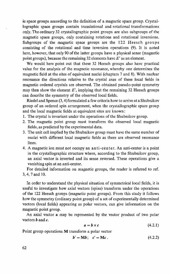
ic space groups according to the definition of a magnetic space group. Crystallographic space groups contain translational and rotational transformations only. The ordinary 32 crystallographic point groups are also subgroups of the magnetic space groups, only containing rotations and rotational inversions. Subgroups of the magnetic space groups are the 122 Heesch groups consisting of the rotational and time inversion operations (9). It is noted here, however, that only 90 of the latter groups have a physical sense (magnetic point groups), because the remaining 32 elements have E' as an element.
We would here point out that these 32 Heesch groups also have practical value for the analysis of the magnetic resonance, whereby one determines the magnetic field at the sites of equivalent nuclei (chapters 7 and 8). With nuclear resonance the directions relative to the crystal axes of these local fields in magnetic ordered crystals are observed. The obtained pseudo-point symmetry may then show the element E', implying that the remaining 32 Heesch groups can describe the symmetry of the observed local fields.
Riedel and Spence (3, 4)formulated a few criteria how to arrive at a Shubnikov group of an ordered spin arrangement, when the crystallographic space group and the local magnetic fields at equivalent sites are known: 1. The crystal is invariant under the operations of the Shubnikov group. 2. The magnetic point group must transform the observed local magnetic
fields, as predicted by the experimental data. 3. The unit cel! implied by the Shubnikov group must have the same number of
nuclei with different local magnetic fields as there are observed resonance lines.
4. A magnetic ion must not occupy an anti-center. An anti-center is a point in the crystallographic structure where, according to the Shubnikov group, an axial vector is inverted and its sense reversed. These operations give a vanishing spin at an anti-center. Por detailed information on magnetic groups, the reader is referred to ref.
3, 4, 7 and 10.
In order to understand the physical situation of symrnetrical local fields, it is useful to investigate how axial vectors (spins) transform under the operations of the 122 Heesch groups (magnetic point groups). From this study it follows how the symmetry ( ordinary point group) of a set of experimentally determined vectors Oocal fields) appearing as polar vectors, can give information on the magnetic point group.
An axial vector a may be represented by the vector product of two polar vectors b and c.
a =bxc
Point group operations M transform a polar vector
b'=Mb; c'=Mc.
62
(4.2.1)
(4.2.2)
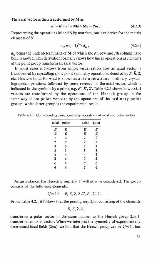
The axial vector is then transformed by M as
a' =b'xc' =MbxMc=Na. (4.2.3)
Representing the operations M and N by matrices, one can derive for the matrix elements of N
. i+Jd nil = ( -1) li, (4.2.4)
d11 being the underdeterminant of Mof which the ith row andjth column have been removed. This derivation formally shows how linear operations as elements of the point group transform an axial vector.
In most cases it follows from simpte visualization how an axial vector is transformed by crystallographic point symmetry operations, denoted by E, E, 2, etc. This also holds for what is known as anti-operations: ordinary crystallograpbic operations followed by sense reversal of the axial vector, which is indicated in the symbols by a prime, e.g. E', E', 2'. Table4.2.l shows how axial vectors are transformed by the operations of the Heesch group in the same way as are pol ar vectors by the operations of the ordinary point group, which latter group is the experimental result.
Table 4.2.1. Corresponding point syrnmetry operations of axial and polar vectors
axial po lar axial po lar
E E E' Ë E E Ë' Ë 2 2 2' 2 2 2 2' 2 3 3 3' 3 3 3 3' 3 4 4 4' 4 4 4 4' 4 6 6 6' ()
() 6 ()' ()
As an instance, the Heesch group 2/m l' will now be considered. The group consists of the following elements:
2/m I': E, E, 2, 2 E', E', 2', 2'.
From Table 4.2.1 it follows that the point group 2/m, consisting of the elements
E,E,2,2,
transforms a polar vector in the same manner as the Heesch group 2/m l' transforms an axial vector. When we interpret the symmetry of experimentally determined local fields (2/m), we find that the Heesch group can be 2/m l', but
63
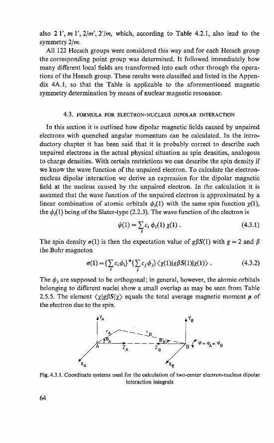
also 2 l', m 1', 2/m', 2'/m, which, according to Table 4.2.1, also lead to the symmetry 2/m.
All 122 Heesch groups were considered this way and for each Heesch group the corresponding point group was determined. lt followed immediately how many different local fields are transformed into each other through the operations of the Heesch group. These results were classified and listed in the Appendix 4A.l, so that the Table is applicable to the aforementioned magnetic symmetry determination by means of nuclear magnetic resonance.
4.3. FORMULA FOR ELECTRON-NUCLEUS DIPOLAR INTERACTION
In this section it is outlined how dipolar magnetic fields caused by unpaired electrons with quenched angular momentum can be calculated. In the introductory chapter it has been said that it is probably correct to describe such unpaired electrons in the actual physical situation as spin densities, analogous to charge densities. With certain restrictions we can describe the spin density if we know the wave function of the unpaired electron. To calculate the electronnucleus dipolar interaction we derive an expression for the dipolar magnetic field at the nucleus caused by the unpaired electron. In the calculation it is assumed that the wave function of the unpaired electron is approximated by a linear combination of atomie orbitals </>;(1) with the same spin function x(l), the <f>t(l) being of the Slater-type (2.2.3). The wave function of the electron is
( 4.3.1)
The spin density a(l) is then the expectation value of gpS(l) with g = 2 and p the Bohr magneton
a(1) ={2::C;</>J*ü::CAA<x(1)1gPS(1)1x(l)). (4.3.2) i j
The 4>; are supposed to be orthogonal; in genera!, however, the atomie orbitals belonging to different nuclei show a small overlap as may be seen from Table 2.5.5. The element <xlgPSlx> equals the total average magnetic moment µ of the electron due to the spin.
Fig. 4.3.1. Coordinate systems used for the calculation of two-center electron-nucleus dipolar interaction integrals
64
a(l) =µLei ei <Pi (1) tPi(l) (4.3.3) i
The spin density caused by </1 1(1) is centered around A, and Bis the nucleus site. The contribution to the total magnetic field at B owing to </J 1(1) is then given by
The x-component of this field is then, for instance,
+3J µ"x~+µyXaYa+µzxaza A.'!"(r 8 <p \A.(r 8 <p \dr 5 'l'i A> A> Al 'l'I A> A• AJ •
1 ra (4.3.5)
Substituting (x8 , y 8 , z 8) into spherical coordinatec;, taking for the </Ji(rA)
quenched orbitals (Tab Ie 2.2.1 ), transforrniog the resulting expression into elliptical coordioates (2A.3.2, Fig. 4.3.1), and using
f2" J 0 sinm <p cosn <p d<p = 0 if mor n odd, (4.3.6)
For Hy(B) and HAB) similar expressioos can be derived. The total field in B, caused by electron 1 can now be obtained by carrying out
the integrations (4.3.7) for all </J; (4.3.1) and adding the integrals properly (4.3.3).
4.4. NUMERICAL CALCULATION OF THE LOCAL FIELD ATA PROTON SITE
IN ANTIFERROMAGNETIC CuC12.2H20
In this section we calculate the local field at a proton position in CuCl2 .2H20, caused by the surrounding magnetically ordered electrons localized around the Cu2 + sites. The proton positions are supposed to be those found by Peterson and Levy (10) by means of neutron diffraction at room temperature. The arrangement of the magnetic moments is assumed to be roughly the one proposed by Poulis and Hardeman (11, 12) which also has been calculated in section 3.5. The canting of about lO % of the electron spins from the easy axis, as has been suggested by Moriya (14, section 3.3), is considered. For the wave
65
function of the unpaired electron we take the wave function approximaied in chapter 2.
The shortest Cu2 + -proton distance is about 5 a.u. The contribution to the magnetic field at the proton site of Cu2 + electrons at more than 25 a. u. has been neglected, inducing an inaccuracy in the result of the calculation of less than one per cent. The spin density at a eu2+ site is, according to the results of the ligand-field treatment (2.8. l, 4.3.3)
a(l) = µ {o.91 dxy+0.31 pn(Cl- l)V2pn(Cl- 4) + 0.18 pn(Cl-2)V2pn(CI-5)r ( 4.4.1)
The dxy is centered around the Cu2 + site and the pn-orbitals are centered around the chlorine sites (Fig. 2.2.2). In section 2.5 the atomie orbitals had to be expressed in u,n and ö-orbitals de:fined in the frame of Fig. 2.5.1. The same is done here. For all the Cu2+ and Cl- ions within 25 a.u. of the proton the dxy and pn-orbitals of (4.4.1) are expressed as linear combinations of u,n and ö-orbitals, defined in the reference frame of Fig. 4.3.1. In this way the spinsµ de:fined in the coordinate system of Fig. 2.2. l can also be expressed as linear combinations of spin components in the (xA, YA• z~ direction.
In the following it is briefiy shown how these transformations were performed. In Fig. 4.3. l are sketched the reference frames; in this Figure A represents the center of the magnetic orbital and B the proton position. For the transformation of the cluster coordinate system (Fig. 2.2.2), i.e. (x0 , y 0 , z0 ), to the coordinate system of the crystallographic structure, i.e. (x, y, z), holds
x0 = -x sin et+z cos et
Yc = x cos et+z sin et
Ze= y' (4.4.2)
et being the angle between the x and x0-axes. For the transformation of the crystallographic coordinate system to the elementary reference frame, 1.e. (xA, YA• z~, in which the integratîons (4.3.7) are carried out, we have
x = -cos<p cos8 xA +sin <p YA +cos<p sin8 zA
y =-sin <p cos8 xA-cos<p YA +sin <p sin8 zA
Z= + cos8 zA. (4.4.3)
All the transformations were carried out using the formulae (4.4.2) and (4.4.3). The local magnetic field in Bis then computed from the formula (4.3.7). The
integrals in (4.3.7) can be generalized to
I(p, q) =J c/>:'(rA, 8A, <PA)3</>i(rA, 8A, <p~ (sin2 8aY(cos2 8a)qd-r. (4.4.4) 1 ra
66
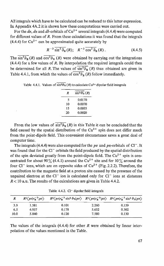
All integrals which have to be calculated can be reduced to this latter expression. In Appendix 4A.2 it is shown how these computations were carried out.
For the du, dn and db-orbitals of Cu2+ several integrals (4.4.4) were computed for different values of R. From these calculations it was found that the integrals (4.4.4) for eu2 + can be approximated quite accurately by
(4.4.5)
The sin2 .9 8 (R) and cos2 .98 (R) were obtained by carrying out the integrations (4.4.4) fora few values of R. By interpolation the required integrals could then
be determined for all R. The values of sin2.98 (R) thus obtained are given in Table 4.4.1, from which the values of cos2 .9 8 (R) follow immediately.
Table 4.4.1. Values of sin20-B (R) to calculate Cu2+ dipolar field integrals
R sin2~(R)
5 0.0170 JO 0.0070 15 0.0035 20 0.0020
From the low values of sin2.98 (R) in this Table it can be concluded that the field caused by the spatial distribution of the Cu2 + spin does not differ much from the point-dipole field. This convenient circumstance saves a great deal of computer time.
The integrals ( 4.4.4) were also computed for the pu and pn-orbitals of ei-. It was found that for the Cl - orbitals the field produced by the spatial distribution of the spin deviated greatly from the point-dipole field. The Cu2 + spin is concentrated for about 90% (4.4.1) around the Cu2+ site and for 10% around the four Cl - ions, which are on opposite si des of Cu2 + (Fig. 2.2.2). Therefore, the contribution to the magnetic field at a proton site caused by the presence of the unpaired electron at the Cl - ion is calculated only for Cl - ions at distances R < 10 a.u. The results of the calculations are given in Table 4.4.2.
Table 4.4.2. CJ- dipolar field integrals
R R4(p<1ir83/p<1) R4(p<1ir8 3 sin2 '!9-B IP<1) R4(pnlrij 3Jp.n) R4(pnJr; 3 sin2 '!9-Blpn)
3.9 1.581 0.101 2.260 0.159 6.5 4.957 0.178 5.632 0.302
10.0 5.840 0.120 7.580 0.130
The values of the integrals (4.4.4) for other R were obtained by linear interpolation of the values mentioned in the Table.
67
All the calculated values of (HxB> H, 8 , Hza) were transformed into the coordinates of the crystallographic structure, the transfonnation matrix being the inverted matrix of (4.4.3). The local field at the proton site is the vector sum of the fields produced by all the unpaired electrons in the crystal. Assuming the spin arrangement proposed by Poulis and Hardeman (11, 12, Fig. 3.4.1) we find the numerical values to be
IHxl = 26,650 A/m (335 Oe)
IH,I = 47,750 A/m (600 Oe)
IHzl = 10,350 A/m (130 Oe).
These values are in poor agreement with the values obtained experimentally by Poulis et al. (13),
IHxl = 42,900 A/m (539 Oe)
IH,I = 30,100 A/m (378 Oe)
IHzl = 30,200 A/m (380 Oe) .
From the calculation it followed that the calculated values are very sensitive to slight changes of direction of the spins of the Cu2+ ions. Tilting the spins 10° off the a-axis in the a,c-plane, Fig. 3.4.1, we find for the Iocal fields
IHxl = 28,600 A/m (360 Oe)
IH,I = 45,000 A/m (565 Oe)
IHzl = 31,800 A/m (400 Oe).
Variation of the proton positions will also give a great change of magnetic field values, because the calculated field values are the net sum of a great number of terms of about the same order of magnitude.
The conclusion is that better agreement between the experimentally determined and the calculated values cannot be reached if the proton positions in CuC12 .2H20 below the Néel point and the spin direction at a Cu2 + ion are not precisely known.
Attention is drawn to the fact that the delocalization of the unpaired electron at the Cl - ions does not strongly affect the calculated values.
Moriya (14) argued that CuCl2 .2H20 has a canted structure, i.e. the spins in one a,c-plane (Fig.3.4.1) are tilted in the positive c-direction, and in an adjacent a,c-plane in the negative c-direction. He supposed that the canting could amount to about 10 %. Contrary what Moriya expected, this canting of the electron spins in CuCl2 .2H20 does not, in our calculation, improve the agreement between calculated and experimental values of the local field.
68
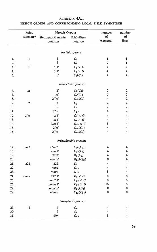
APPENDIX 4A. I HEESCH GROUPS AND CORRESPONDING LOCAL FIELD SYMMETRIES
Point Heesch Groups number number symmetry Hermann-Mauguin Schönfliess of of
notation notation elements lines
triclinic system :
1. 1 C1 2. I C1 2
3. ï 1 1' C1 x G 2 2 4. I 1' C1 x G 4 2 5. 1' C1(C1) 2 2
monoc/inic system:
6. m 2' C2(C1) 2 2 7. m' Cs(C1) 2 2 8. 2'/m' C21i(C1) 4 2
9. 2 2 C2 2 2 10. m Cs 2 2 11 . 2/m C2" 4 2 12. 2/m 2 1' C2 x G 4 4 13. ml' C, x G 4 4 14. 2/m 1' C211 x G 8 4 15. 2/m' C2"(C2) 4 4 16. 2'/m C21i(C,) 4 4
orthorhombic system:
17. mm2 m'm'2 C2v(C2) 4 4 18. mm'2' C2v(C,) 4 4 19. 22'2' Da(C2) 4 4 20. mm'm' D21,(C2v) 8 4
21. 222 222 Da 4 4 22. mm2 Cav 4 4 23. mmm Da1i 8 4
24. mmm 2221' Da X G 8 8 25. mm2 l' Cav X G 8 8 26. mmml' Da" x G 16 8 27. m'm'm' Da1i(D2) 8 8 28. m'mm C2"(C2v) 8 8
tetragonal system:
29. 4 4 C4 4 4 30. 4 S4 4 4 31. 4/m c4h 8 4
69
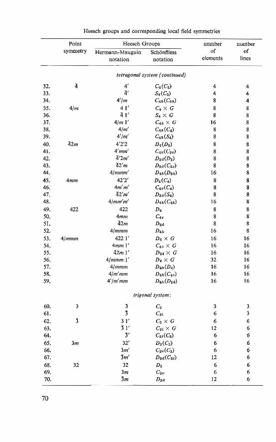
Heesch groups and corresponding local field symmetries
Point Heesch Groups number number symmetry Hermann-Mauguin Schönfliess of of
notation notation elernents lines
tetragonal system ( continued)
32. 4' C4(C2) 4 4 33. 4' S4(C2) 4 4 34. 4'/m Co(C2") 8 4 35. 4/m 4 1' C4 x G 8 8 36. 4 1' S4 x G 8 8 37. 4/m 1' C4" x G 16 8 38. 4/m' C4"(C4) 8 8 39. 4'/m' C4"(S4) 8 8 40. 42m 4'2'2 D4(D2) 8 8 41. 4'mm' C4v(C2v) 8 8 42. 4'2m' D2ct(D2) 8 8 43. 42'm D2ct(C2v) 8 8 44. 4/mmm' D4h(D21>) 16 8 45. 4mm 42'2' D4(C4) 8 8 46. 4 ' I mm C4v(C4) 8 8 47. 42'm' D2ct(S4) 8 8 48. 4/mm'm' D41>(C41i) 16 8 49. 422 422 D4 8 8 50. 4mm C4v 8 8 51. 42m Dart 8 8 52. 4/mmm D4n 16 8 53. 4/mmm 4221 ' D4 x G 16 16 54. 4mm l' C4v x G 16 16 55. 42m 1' D2rt x G 16 16 56. 4/mmm 1' D4 x G 32 16 57. 4/mmm D4h(D,V 16 16 58. 4/m'mm D4h(C4V) 16 16 59. 4'/m'mm D4"(D2rt) 16 16
trigonal system:
60. 3 3 Ca 3 3 61. 3 Cst 6 3
62. 3 3 1' Cs x G 6 6 63. 3 l' Cai x G 12 6 64. 3' Cs;(Ca) 6 6
65. 3m 32' Da(Ca) 6 6 66. 3m' Csv(Cs) 6 6 67. 3m' Dact(Ca1) 12 6
68. 32 32 Ds 6 6 69. 3m Cav 6 6 70. 3m Dart 12 6
70
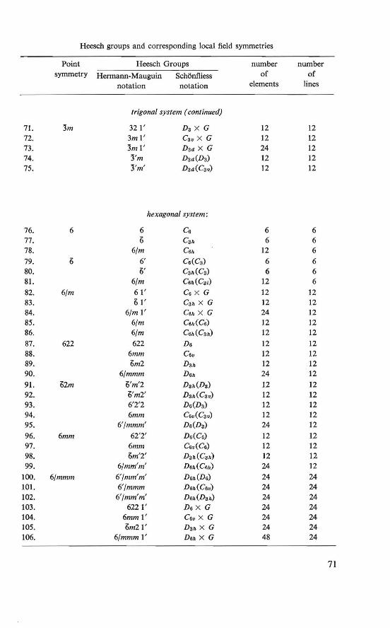
Heesch groups and corresponding local field symmetries
Point Heesch Groups nwnber nwnber symmetry Herrnann-Mauguin Schönfiiess of of
notation notation elements lines
trigonal system ( continued)
71. 3m 32 1' Ds X G 12 12 72. 3m 1' Cav X G 12 12 73. 3m l ' Daa X G 24 12 74. 3'm Dsa(Da) 12 12 75. 3'm' Daa(Cav) 12 12
hexagonal system:
76. 6 6 Cs 6 6 77. 0 Cah 6 6 78. 6/m Csh 12 6 79. 6' Cs(Ca) 6 6 80. o' Cs11(Cs) 6 6 81. 6/m Csh(CaJ) 12 6 82. 6/m 6 1' Cs x G 12 12 83. 0 l ' Ca11 x G 12 12 84. 6/m 1' Csh x G 24 12 85. 6/m Cs11(Cs) 12 12 86. 6/m Cs11(Ca11) 12 12 87. 622 622 Da 12 12 88. 6mm Cav 12 12 89. om2 Ds11 12 12 90. 6/mmm Dah 24 12
91. o2m o'm'2 Dah(Ds) 12 12 92. o'm2' Dsh(Csv) 12 12 93. 6'2'2 Ds(Da) 12 12 94. 6mm Csv(Cav) 12 12 95. 6'/mmm' Ds(Da) 24 12
96. 6mm 62'2' Ds(Cs) 12 12 97. 6mm Csv(Cs) 12 12 98. om'2' Da11(Ca11) 12 12 99. 6/mm'm' Ds11(Cs11) 24 12
100. 6/mmm 6'/mm'm' Dah(Ds) 24 24 101. 6'/mmm Dsh(Csv) 24 24 102. 6'/mm'm' Dsh(Da11) 24 24 103. 6221 ' Da x G 24 24 104. 6mm 1' Cav X G 24 24 105. om21 ' Ds11 x G 24 24 106. 6/mmm 1' Da11 x G 48 24
71
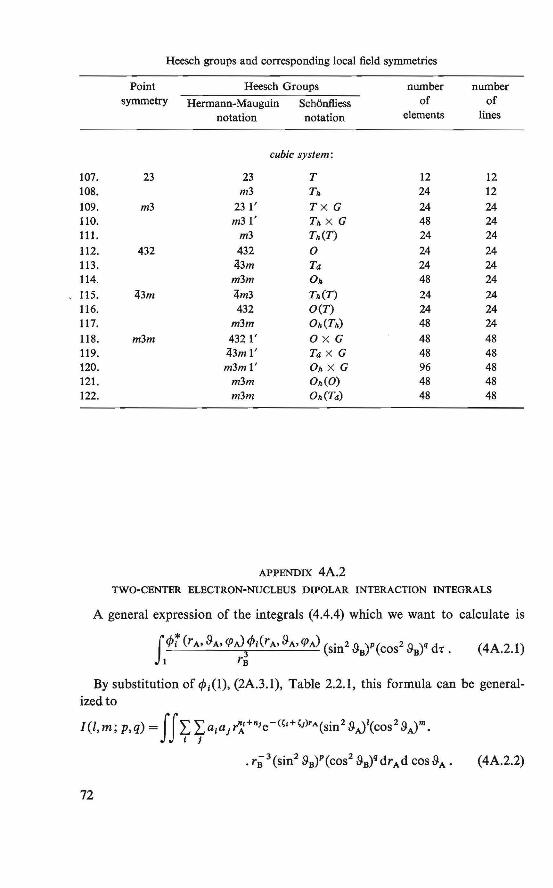
Heesch groups and corresponding Jocal field symmetries
Point Heesch Groups number number symmetry Hermann-Mauguin Schönfliess of of
notation notation elements lines
cubic system:
107. 23 23 T 12 12 108. m3 Tn 24 12 109. m3 23 l' Tx G 24 24 110. m3 l' T1o x G 48 24 lll. m3 T1o(T) 24 24 ll2. 432 432 0 24 24 113. 43m Ta 24 24 ll4. m3m o" 48 24 115. 43m 4m3 T"(T) 24 24 ll6. 432 O(T) 24 24 117. m3m O"(T1o) 48 24 118. m3m 432 1' OXG 48 48 119. 43m 1' Ta x G 48 48 120. m3ml' o" x G 96 48 121. m3m O"(O) 48 48 122. m3m O"(Ta) 48 48
APPENDIX 4A.2 TWO-CENTER ELECTRON-NUCLEUS DIPOLAR INTERACTION INTEGRALS
A genera! expression of the integrals (4.4.4) which we want to calculate is
J<fi (r A> 8A, <pJJ</>,(r A• 8A, <pJ (sin2 ~)P(cos2 ~)q d-r. 1 r8
(4A.2.l)
By substitution of </>1(1), (2A.3.1), Table 2.2.1, this formula can be generalized to
I(l,m; p,q) = J J ~ ~a1 a1 r~+n1e-<~i+ÇJ)'A(sin2 8J1(cos 2 8Jm.
(4A.2.2)
72
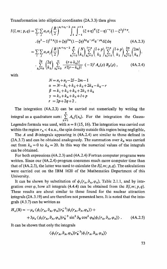
Transformation into elliptical coord.inates (2A.3.3) then gives
(4A.2.3)
(R)n1+n1-2 N (N) l+p (l+p) l+p (l+p) 2m (2m)
= IIa·a· - I I I I i j • J 2 k1=0 k1 k1=0 k2 k3=0 k3 k4=0 k4 .
lq (2q) 00
(r+k6)! Y . k,"'fo ks k"[;.O r!(r-k6)! (-1) A"(p) Bp(P), (4A.2.4)
with N = n1+n1-21-2m-1 a =N-k1+k2+k3+2k4 -k6 -r f3 = k1 +k2 +k3 +2k5 +k6
y =k3+k4 +k5 +l+p r =2p+2q+2.
The integration (4A.2.3) can be carried out numerically by writing the n
integral as a quadrature sum: I AJ(xJ. For the integration the Gauss-k= 1
Legendre formula was used, with n = 8 (15, 16). The integration was carried out within the region r A < 4 a.u., the spin density outside this region being negligible.
The A and B-integrals appearing in (4A.2.4) are similar to those defined in (2A.3.7) and can be obtained analogously. The summation over k 6 was carried out from k 6 = 0 to k 6 = 20. In this way the numerical values of the integrals can be obtained.
For both expressions (4A.2.3) and (4A.2.4) Fortran computer programs were written. Since our (4A.2.4)-program consumes much more computer time than that of (4A.2.3), the Jatter was used to calculate the /(/,m; p,q). The calculations were carried out on the IBM 1620 of the Mathematics Department of this University.
It can be shown by substitution of </> 1(rA,8A,<f>A), Table 2.1.1, and by integration over <p, how all integrals (4.4.4) can be obtained from the /(/,m; p,q). These results are about similar to those found for the nuclear attraction integrals (2A.3.19) and are therefore not presented here. It is noted that the integrals (4.3.7) can be written as
Hx(B) = - µx (</>1(r A• 8A, cpJlrä 3 1</>i(rA, 8A> cpJ) +
+3µx (</>1(r A• 8A, cpJlrä 3 sin2 8B cos2 <t>Bl</>1(r A• 8A, q>J) . (4A.2.5)
It can be shown that only the integrals
«f>1(r A> 8A> q>Jlrä 3 1</>i(r A• 8A, q>J)
73
and (4A.2.6)
need to be calculated and the other integrals can be derived from these.
REFERENCES
1. G. E. Pake, J. Chem. Phys., 16 (1948) 327. 2. V. Jaccarino, Magnetism l/A, p. 307 (G.T. Rado and H. Suhl,eds.),Academic Press, New
York and London (1965). 3. E. P. Riedel and R. D. Spence, Physica, 26 (1960) 1174. 4. E. P. Riedel, Ph.D. Thesis, Michigan State University (1961). 5. A. M. Zamorzaev, Soviet Physics Cryst., 3 (1958) 401. 6. N.V. Belov, N.N. Neronova and T. S. Srnirnova, Soviet Physics Cryst., 2 (1957) 311. 7. W. Opechowsky and Rosalia Guccione, Magrtetism IIA , p. 105 (G. T. Rado and H. Suhl,
eds.), Academie Press, New York and London (1965). 8. R. D . Spence, The Mortoclirtic and Orthorhombic Shubrtikov Groups, Unpublished Report,
Michigan State University (1963). 9. H. Heesch, Z. Krist., 73 (1930) 325.
10. R. R. Birss, Symmetry and Magrtetism, North-Holland Publishing Company, Amsterdam (1964).
11. N . J. Poulis and G. E.G. Hardeman, Physica, 18 (1952) 201. 12. G . Shirane, B. C. Frazer and S. A. Friedberg, Phys. Letters, 17 (1965) 95. 13. N. J. Poulis, G . E.G. Hardeman, W. van der Lugt and W. P.A. Hass, Physica, 24 (1958)
280. 14. T. Moriya, Phys. Rev., 120 (1960) 91. 15. V.I. Krylov, Approximate Calculation of lntegrals, The Macmillan Company, New York
(1962). 16. Z. Kopal, Numerical Analysis, Chapman and Hall, Ltd., London (1955).
74
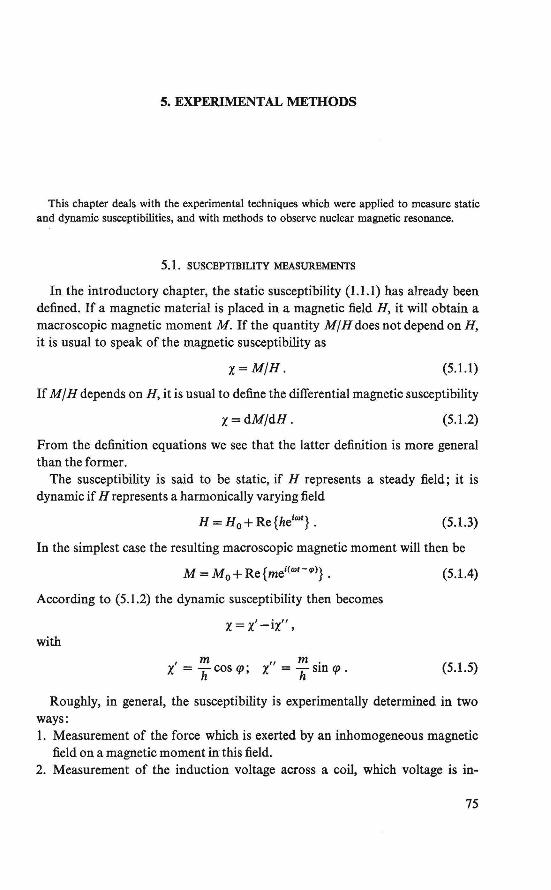
5. EXPERIMENTAL METHODS
This chapter deals with the experimental techniques which were applied to measure statie and dynamic susceptibilities, and with methods to observe nuclear magnetic resonance.
5.1. SUSCEPTIBILITY MEASUREMENTS
In the introductory chapter, the statie susceptibility (l.1.1) bas already been defined. If a magnetic material is placed in a magnetic field H, it will obtain a macroscopie magnetic moment M. If the quantity M / H does not depend on H, it is usual to speak of the magnetic susceptibility as
x=M/H. (5.1.1)
If M/H depends on H, it is usual to define the differential magnetic susceptibility
x=dM/dH. (5.1.2)
From the definition equations we see that the latter definition is more general than the former.
The susceptibility is said to be statie, if H represents a steady field; it is dynamic if H represents a harmonically varying field
(5.1.3)
In the simplest case the resulting macroscopie magnetic moment will then be
M = M0+ Re{mei(Q)t-q>)}. (5.1.4)
According to (5.1.2) the dynamic susceptibility then becomes
x = x'-ix", with
' m " m . X = h COS <p; X = h Slll <p • (5.1.5)
Roughly, in genera!, the susceptibility is experimentally deterrnined in two ways: l. Measurement of the force which is exerted by an inhomogeneous magnetic
field on a magnetic moment in this field. 2. Measurement of the induction voltage across a coil, which voltage is in-
75
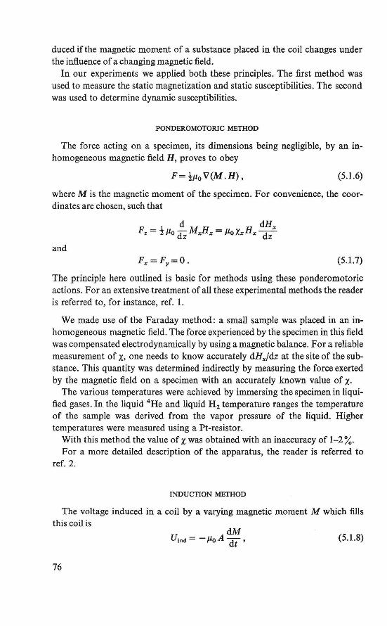
du eed if the magnetic moment of a substance placed in the co il changes under the infl.uence of a changing magnetic field.
In our experiments we applied both these principles. The first method was used to measure the statie magnetization and statie susceptibilities. The second was used to determine dynamic susceptibilities.
PONDEROMOTORIC METHOD
The force acting on a specimen, its dimensions being negligible, by an inhomogeneous magnetic field H, proves to obey
F= !µ0 V(M .H), (5.1.6)
where M is the magnetic moment of the specimen. For convenience, the coordinates are chosen, such that
and Fx=Fy=O. (5.1.7)
The principle here outlined is basic for methods using these ponderomotoric actions. For an extensive treatment of all these experimental methods the reader is referred to, for instance, ref. l.
We made use of the Faraday method: a small sample was placed in an inhomogeneous magnetic field. The force experienced by the specimen in this field was compensated electrodynarnically by using a magnetic balance. Fora reliable measurement of x, one needs to know accurately dHxf dz at the site of the substance. This quantity was determined indirectly by measuring the force exerted by the magnetic field on a specimen with an accurately known value of X·
The various temperatures were achieved by immersing the specimen in liquified gases. In the liquid 4 He and liquid H 2 temperature ranges the temperature of the sample was derived from the vapor pressure of the liquid. Higher temperatures were measured using a Pt-resistor.
With this method the value of x was obtained with an inaccuracy of 1-2 %. For a more detailed description of the apparatus, the reader is referred to
ref. 2.
INDUCTION METHOD
The voltage induced in a coil by a varying magnetic moment M which fills this coil is
(5.1.8)
76
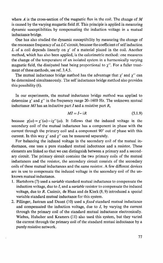
where A is the cross-section of the magnetic flux in the coil. The change of M
is caused by the varying magnetic field H. This principle is applied in measuring dynamic susceptibilities by compensating the induction voltage in a mutual inductance bridge.
One has also studied the dynamic susceptibility by measuring the change of the resonance frequency of an LC circuit, because the coefficient of self induction L of a coil depends linearly on x' of a material placed in the coil. Another method, which has also been applied, is the calorimetrie method: one measures the change of the temperature of an isolated system in a harmonically varying magnetic field, the dissipated heat being proportional to x". Fora fuller treatment of these methods, see ref. 3,4,5.
The mutual inductance bridge method has the advantage that x' and x" can be determîned simultaneously. The self inductance bridge method also provides this possibility (6).
In our experiments, the mutual inductance bridge method was applîed to determine x' and x" in the frequency range 20-1600 Hz. The unknown mutual inductance MI has an inductive part I and a resistive part R,
Ml=l-iR (5.1.9)
because x(m) = x'(m)-ix"(m). It follows that the induced voltage in the secondary coil of the mutual inductance has a component in phase with the current through the primary coil and a component 90° out of phase with this current. In this way x' and x" can be measured separately.
For balancing the induced voltage in the secondary coil of the mutual inductance, one uses a pure standard mutual inductance and a resistor. These elements are linked so that we can distinguish between a primary and a secondary circuit. The primary circuit contains the two primary coils of the mutual inductances and the resistor, the secondary circuit consists of the secondary coils of these mutual inductances and the .same resistor. A few different devices are in use to compensate the induced voltage in the secondary coil of the unknown mutual inductance. 1. Hartshom (7) used a variable standard mutual inductance to compensate the
induction voltage, due to /, and a variable resistor to compensate the induced voltage, due to R. Casimir, de Haas and de Klerk (8, 9) introduced a special variable standard mutual inductance for this system.
2. Pillinger, Jastram and Daunt (10) used afixed standard mutual inductance and compensated the induction voltage, due to /, by varying the current through the primary coil of the standard mutual inductance electronically. Wiebes, Hulscher and Kramers (11) also used this system, but they varied the current through the primary coil of the standard mutual inductance by a purely resistive network.
77
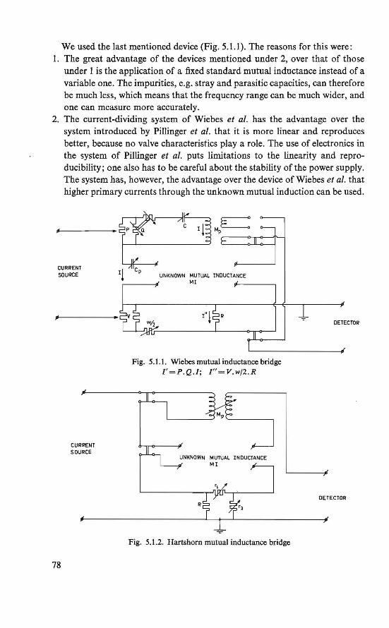
We used the last mentioned device (Fig. 5.1.1). The reasons for this were: 1. The great advantage of the devices mentioned under 2, over that of those
under 1 is the application of a fixed standard mutual inductance instead of a variable one. The impurities, e.g. stray and parasitic capacities, can therefore be much less, which means that the frequency range can be much wider, and one can measure more accurately.
2. The current-dividing system of Wiebes et al. bas the advantage over the system introduced by Pillinger et al. that it is more linear and reproduces better, because no valve characteristics play a role. The use of electronics in the system of Pillinger et al. puts limitations to the linearity and reproducibility; one also bas to be careful about the stability of the power supply. The system has, however, the advantage over the device of Wie bes et al. that higher primary currents through the unknown mutual induction can be used.
CURRENT SOURCE
78
CURRENT SOURCE
UNKNOWN MUTUAl INDUCTANCE MI
Fig. 5.1.1. Wiebes mutual inductance bridge l'=P.Q.l; l"=V.w/2.R
MUTUAL INDUCTANCE MI
R
Fig. 5.1.2. Hartsborn mutual inductance bridge
DETECTOR
DETECTOR
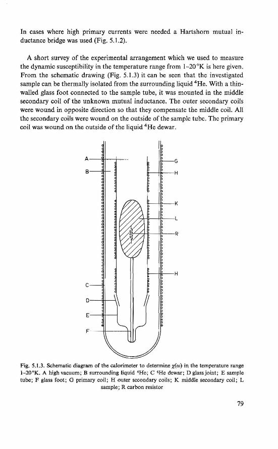
In cases where high primary currents were needed a Hartshorn mutual inductance bridge was used (Fig. 5.1.2).
A short survey of the experimental arrangement which we used to measure the dynamic susceptibility in the temperature range from l-20°K is here given. From the schematic drawing (Fig. 5.1.3) it can be seen that the investigated sample can be thermally isolated from the surrounding liquid 4He. With a thinwalled glass foot connected to the sample tube, it was mounted in the middle secondary coil of the unknown mutual inductance. The outer secondary coils were wound in opposite direction so that they compensate the middle coil. All the secondary coils were wound on the outside of the sample tube. The primary coil was wound on the outside of the liquid 4 He dewar.
Fig. 5.1.3. Schernatic diagram of the calorimeter to determine x(m) in the ternperature range 1-20°K. A high vacuum; B surrounding liquid 4He; C 4He dewar; D glassjoint; E sample tube; F glass foot; G primary coil; H outer secondary coils; K middle secondary coil; L
sample; R carbon resistor
79
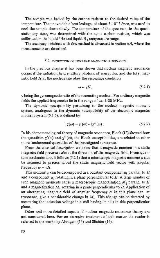
The sample was heated by the carbon resistor to the desired value of the temperature. The unavoidable heat leakage, of about 5. 10- 4 J/sec, was used to cool the sample down slowly. The temperature of the specimen, in the quasistationary state, was determined with the same carbon resistor, which was calibrated in the liquid 4 He and liquid H2 temperature range.
The accuracy obtained with this method is discussed in section 6.4, where the measurements are described.
5.2. DETECTION OF NUCLEAR MAGNETIC RESONANCE
In the previous chapter it has been shown that nuclear magnetic resonance occurs if the radiation field emitting photons of energy liw, and the total magnetic field H at the nucleus site obey the resonance condition
w = yH' (5.2.1)
y being the gyromagnetic ratio of the resonating nucleus. For ordinary magnetic fields the applied frequencies !ie in the range of ca. 1-80 MHz.
The dynamic susceptibility pertaining to the nuclear magnetic moment system, analogous to the dynamic susceptibility of the electronic magnetic moment system (5.1 .5), is defined by
' x(w) = x'(w)-ix"(w). (5.2.2)
In bis phenomenological theory of magnetic resonance, Bloch (12) showed how the quantities x'(w) and x"(w), the Bloch susceptibilities, are related to other more fundamental quantities of the investigated substance.
From the classica1 description we know that a magnetic moment in a statie magnetic field precesses about the direction of the magnetic field. From quantum mechanics too, it follows (5.2.1) that a microscop~c magnetic momentµ can be assumed to precess about the statie magnetic field vector with angular frequency w = yH.
This momentµ can be decomposed in a constant component µ 11 parallel to H and a component µl. rotating in a plane perpendicular to H. A large number of such magnetic momeots cause a macroscopie magnetization M 11 parallel to H and a magnetization Ml. rotating in a plane perpendicular to H. Application of an alteroating magnetic field of angular frequency w in this plane can, at resonance, give a considerable change in Ml.. This change can be detected by measuring the induction voltage in a coil having its axis in this perpendicular plane.
Other and more detailed aspects of nuclear magnetic resonance theory are not considered here. For an extensive treatment of this matter the reader is referred to the works by Abragam (13) and Slichter (14).
80
According to the principles here outlined one may, in genera!, distinguish between two detection techniques: 1. Single-coil system: Measurement of the change in impedance of a coil, when
resonance occurs. This can be easily seen from (5.2.2), because
iroL(ro) = iroL0 x' (ro) + wL0 x" (ro) . (5.2.3)
We may say that this impedance contains a dispersive part iroL0x' (w) and an absorption part wL0x'' (w). These quantities can be measured by electronic means. The system bas first been used by Purcell and co-workers (15).
2. Crossed-coil system: In this device the high-frequency field is produced by the transmitter coil. The induction voltage due to the change in Mi occurring near the resonance frequency in the receiving coil, is detected. This method bas been introduced by Bloch and co-workers (16).
Both methods have comparable application possibilities. The Jatter method can give a little more information. The simplicity of the first method, using one coil, makes it more attractive, especially, when one works at low temperatures. In our experiments the single-coil system was used.
The single-coil method can be realized in several ways, whicb fall into two essentially different categories: steady-state detection techniques and transienteffect detection techniques.
a. Steady-state detection techniques
Q-meter method This device was introduced by Rollin (17) in 1946. The principle is: The high
frequency field in the coil of a tuned LC circuit is fed by a constant-current source. If resonance occurs, the voltage across the circuit changes. The voltage change can be detected. In first approximation it is proportional to Qx", Q being the quality factor of the tuned circuit. The voltage change is small compared with the voltage across the circuit.
Bridge method This arrangement was first used by Purcell, Torrey and Pound (15) in 1946,
and modified by Bloembergen, Purcell and Pound (18). In this metbod, two identical tuned circuits are fed in parallel by a high-frequency signa! generator. The coil of one of these circuits contains the investigated material placed in the steady magnetic field. The output voltage of these circuits are subtracted and amplified. One can derive that this voltage is proportional to x' sin <p- x" cos <p,
<p being the phase angle between the two output voltages of the tuned circuits. By adjusting the bridge it is pos si bie to detect either x' or x".
Marginal oscillator method The system was first used by Pound (19) in 1947. The oscillator is tuned by an
81
LC circuit. The sample is placed in the coil with se!f inductance L. The level of oscillation depends strongly on the load of the tuning circuit. The change in oscillation level is strongest when the oscillation level is lowest (marginal). The modulation of the amplitude depends in first instance on x" and the resonance frequency shift on x'. Hence, application of amplitude modulation detection gives a signa! proportional to x" and frequency modulation detection gives a signa! proportional to x' (20).
b. Transient-effect detection techniques
Superregenerative method This system was first applied by Roberts (21) in 1947. The oscillator is tuned
by an LC circuit, in the coil ofwhich the sample is placed. The osci!lation grows and decays which is general!y contro!led by a quench oscillator. The spectrum of the oscillations then consists of a centra! frequency and two sideband frequencies, which gives a very complicated resonance pattem. The detection of the signa! is roughly analogous to the way described for the marginal oscillator.
Pu/se method In this method the higb-frequency field is modulated by a sharp pulse which
induces transitions in the nuclear system. This method is especially of advantage if one is interested in the measurement of relaxation times. lt was first described by Torrey (22) in 1949 and by Hahn (23) in 1950.
In the first four methods the steady magnetic field can be modulated slowly (e.g. 50 Hz) with an amplitude of about 2500 A/m to display the resonance line while the frequency is kept constant. When the steady field is close to the resonance value, the total field obeys the resonance condition twice each cycle (5.2.1 ). After amplification and detection the resonance line can then be displayed on an oscillograph.
For further information about these detecting systems the reader is referred to e.g. ref. 20, 24 and 25.
We are interested in the displacement of the resonance lines of a nucleus in a solid relative to the resonance line of the free nucleus (chapter 4). This displacement is of the order of 105 A/m. The resonance-line width is about 500 A/m. Operating frequencies are generally of 4-20 MHz; applied magnetic field: 0--5. 105 A/m.
In our experiments, the marginal oscillator method was used. Arguments were: 1. lt is electronical!y simpler than the other devices mentioned. 2. lt does not need very accurate adjustment, as is required in the case of the
bridge methods.
82
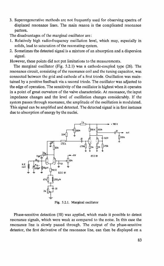
3. Superregenerative methods are not frequently used for observing spectra of displaced resonance lines. The main reason is the complicated resonance pattern.
The disadvantages of the marginal oscillator are: 1. Relatively high radio-frequency oscillation level, which may, especially in
solids, lead to saturation of the resonating system. 2. Sometimes the detected signa! is a mixture of an absorption and a dispersion
signa!. However, these points did not put lim.itations to the measurements.
The marginal oscillator (Fig. 5.2. l) was a cathode-coupled type (26). The resonance circuit, consisting of the resonance coil and the tuning capacitor, was connected between the grid and cathode of a first triode. Oscillation was maintained by a positive feedback via a second triode. The oscillator was adjusted to the edge of operation. The sensitivity of the oscillator is highest when it operates in a point of great curvature of the valve characteristic. At resonance, the input impedance changes and the level of oscillation changes considerably. If the system passes through resonance, the amplitude of the oscillation is modulated. This signa! can be amplified and detected. The detected signa! is in first înstance due to absorption of energy by the nuclei.
1 k
Fig. 5.2.1. Marginal oscillator
Phase-sensitive detection (18) was applied, which made it possible to detect resonance signals, which were weak as compared to the noise. In thîs case the resonance line is slowly passed through. The output of the phase-sensitive detector, the first derivative of the resonance line, can then be displayed on a
83
recorder. A further advantage of this recording system is the automatic operation of the apparatus.
REFERENCES
1. L. F. Bates, Modern Magnetism, Cambridge Univ. Press, London and New York (1961). 2. H. M. Gijsman, Thesis, Leiden (1958). 3. C. J. Gorter, Paramagnetic Relaxation, Elsevier Publishing Company, Amsterdam (1947). 4. L. J. F. Broer, Thesis, Amsterdam (1946). 5. L. J. Dijkstra, Thesis, Amsterdam (1943). 6. B. Hague, Alternating Current Bridge Methods, Sir Isaac Pitman and Sons, Ltd., London
(1955). 7. L. Hartshom, J. Sci. Instr., 2 (1925) 145. 8. H. B. G. Casimir, W. J. de Haas and D. de Klerk, Physica, 6 (1939) 241. 9. D. de Klerk, Thesis, Leiden (1948).
10. W. L. Pillinger, P. S. Jastram and J. G. Daunt, Rev. Sci. Instr" 29 (1958) 159. 11. J. Wiebes, W. S. Hulscher and H.C. Kramers, Appl. Sci. Res" UB (1965) 213. 12. F. Bloch, Phys. Rev" 70 (1946) 460. 13. A. Abragam, Nuclear Magnetism, Oxford Univ. Press, London (1961). 14. C. P. Stichter, Principles of Magnetic Resonance, Harper and Row, New York, Evanston
and London (1963). 15. E. M. Purcell, H.C. Torrey and R. V. Pound, Phys. Rev., 69 (1946) 37. 16. F. Bloch, W. W. Hansen and M. Packard, Phys. Rev" 69 (1946) 127; 70 (1946) 474. 17. B. V. Rollin, Nature, London, 158 (1946) 669. 18. N. Bloembergen, Thesis, Leiden (1948); Nuclear Magnetic Relaxation, W. A. Benjamin,
Ine., New York (1961). 19. R. V. Pound, Phys. Rev" 72 (1947) 527. 20. R. V. Pound, Progress in Nuclear Physics 2, p. 21 (0. R. Frisch ed.) Pergamon Press, Ltd.,
London (1952). 21. A. Roberts, Rev. Sci. lnstr" 18 (1947) 845. 22. H.C. Torrey, Phys. Rev., 76 (1949) 1059. 23. E. L. Hahn, Phys. Rev" 80 (1950) 580. 24. E. R. Andrew, Nuclear Magnetic Resonance, Cambridge Univ. Press, London and New
York (1958). 25. D.J.E. Ingram, Spectroscopy at Radio and Microwave Frequencies, Butterworths Scientific
Publications, London (1955). 26. J. A. Cowen and W. H. Tantilla, Am. J. Phys., 26 (1958) 381.
84
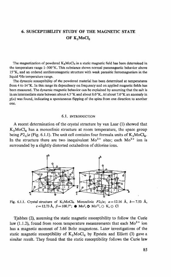
6. SUSCEPTIBILITY STUDY OF THE MAGNETIC STATE
OF K3MoCl6
. The magnetization of powdered KaMoCls in a statie magnetic field bas been detennined in the temperature range l-300°K. This substance shows normal paramagnetic behavior above 15°K, and an ordered antiferromagnetic structure with weak parasitic ferromagnetism in the liquid 4He temperature range.
The dynamic susceptibility of the powdered material has been determined at temperatures from 4 to 14 °K. In this range its dependency on frequency and on applied magnetic fields has been measured. The dynamic magnetic behavior can be explained by assuming that the salt is in an intermedia te state between about 4.5 °K and about 8.0 °K. At about 7 .0 °K an anomaly in x(w) was found, indicating a spontaneous flipping of the spins from one direction to another one.
6.1. INTRODUCTION
A recent determination of the crystal structure by van Laar (1) showed that K 3MoC16 bas a monoclinic structure at room temperature, the space group being P2ifa (Fig. 6. l.l}. The unit cell contains four formula units of K 3MoCl6 •
In the structure there are two inequivalent Mo3+ sites; each Mo3 + ion is surrounded by a slightly distorted octahedron of chlorine ions.
b b
Fig. 6.1.1. Crystal structure of KaMoCI@. Monoclinic P21/a; a=12.16 A, b=7.53 A, c= 12.73 A, P= 108.7°; • Mol, O Mon, O K, O Cl
Tjabbes (2), assuming the statie magnetic susceptibility to follow the Curie law (1.1.2), found from room temperature measurements that each Mo3 + ion bas a magnetic moment of 3.66 Bohr magnetons. Later investigations of the statie magnetic susceptibility of K 3MoCl6 by Epstein and Elliott (3) gave a similar result. They found that the statie susceptibility follows the Curie law
85
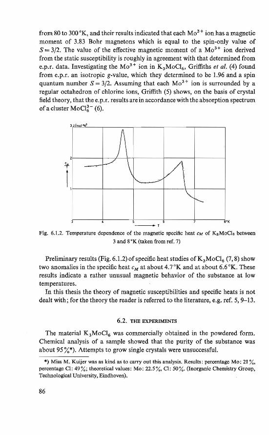
from 80 to 300 °K, and their results indicated that each Mo3 + ion has a magnetic moment of 3.83 Bohr magnetons which is equal to the spin-only value of S = 3/2. The value of the effective magnetic moment of a Mo3+ ion derived from the statie susceptibility is roughly in agreement with that determined from e.p.r. data. Investigating the Mo3+ ion in K 3MoCl 6 , Griffiths et al. (4) found from e.p.r. an isotropic g-value, which they determined to be 1.96 and a spin quantum number S = 3/2. Assuming that each Mo3 + ion is surrounded by a regular octahedron of chlorine ions, Griffith (5) shows, on the basis of crystal field theory, that the e.p.r. results are in accordance with the absorption spectrum of a cluster MoCl~ - (6).
)J m 1 1
2r--~~~-t-~r--1--+-~~~---t~~~~+-~~____,
5f
î 1r--~~~-t-~~~--+-~~~---t~~~~+--~~------i
8°K
Fig. 6.1.2. Temperature dependence of the magnetic specific heat CM of KaMoCla between
3 and 8 °K (taken from ref. 7)
Preliminary results (Fig. 6.1.2) of specific heat studies of K 3MoCl6 (7, 8) show two anomalies in the specific heat c M at about 4. 7 °K and at about 6.6 °K. These results indicate a rather unusual magnetic behavior of the substance at low temperatures.
In this thesis the theory of magnetic susceptibilities and specific heats is not dealt with; for the theory the reader is referred to the Iiterature, e.g. ref. 5, 9-13.
6.2. THE EXPERIMENTS
The material K 3MoCl6 was commercially obtained in the powdered form. Chemical analysis of a sample showed that the purity of the substance was about 95 %*). Attempts to grow single crystals were unsuccessful.
•)Miss M. Kuijer was as kind as to carry out this analysis. Results: percentage Mo: 21 %, percentage Cl: 49%; theoretica] values: Mo: 22.5%, Cl: 50%. (lnorganic Chemistry Group, Technological University, Eindhoven).
86
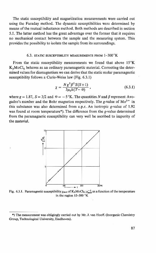
The statie susceptibility and magnetization measurements were carried out using the Faraday method. The dynamic susceptibilities were determined by means of the mutual inductance method. Both methods are described in section 5.1. The Jatter method has the great advantage over the former that it requires no mechanica) contact between the sample and the measuring system. This provides the possibility to isolate the sample from its surroundings.
6.3. STATIC SUSCEPTiBILITY MEASUREMENTS FROM l-300°K
From the statie susceptibility measurements we found that above 15 °K K3 MoC16 behaves as an ordinary paramagnetic material. Correcting the determined values for diamagnetism we can derive that the statie molar paramagnetic susceptibility follows a Curie-Weiss law (Fig. 6.3.1)
Ng 2 /J 2 S(S+l) X = 3µ0k(T- 0) ' (6.3.1)
where g = 1.87, S = 3/2 and e = -5 °K. The quantities N and {J represent Avogadro's number and the Bohr magneton respectively. The g-value of Mo3+ in this substance was also determined from e.p.r. An isotropic g-value of 1.92 was found at room temperature*). The difference from the g-value determined from the paramagnetic susceptibility can very well be ascribed to impurity of the material.
\S.-----,-----.....,.-------.,,
100 200 300°K --+r
Fig. 6.3.1. Paramagnetic susceptibility Xmo1 of KaMoCls; x;;;~1 as a function of the temperature in the region 1 S-300 °K
*)The measurement was obligingly carried out by Mr. J. van Hooff. (lnorganic Chemistry Group, Technologica! University, Eindhoven).
87
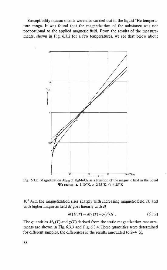
SusceptibUity measurements were also carried out in the liquid 4 He temperature range. lt was found that the magnetization of the substance was not proportional to the applied magnetic field. From the results of the measurements, shown in Fig. 6.3.2 for a few temperatures, we see that below about
20~---------------,--------,
25 50 75 - - --H
1óo.1o'A/m
Fig. 6.3.2. Magnetization Mmo! of K3 MoCls as a function of the rnagnetic field in the liquid 4He region; À 1.10°K, 6. 2.55 °K, O 4.25°K
105 A/m the magnetization rises sharply with increasing magnetic field H, and with higher magnetic field M goes linearly with H
M(H,T) = M 0 (T)+x(T)H. (6.3.2)
The quantities M 0 (T) and x(T) derived from the statie magnetization measurements are showri in Fig. 6.3.3 and Fig. 6.3.4. These quantities were determined for different samples, the differences in the results amounted to 2-4 %:
88
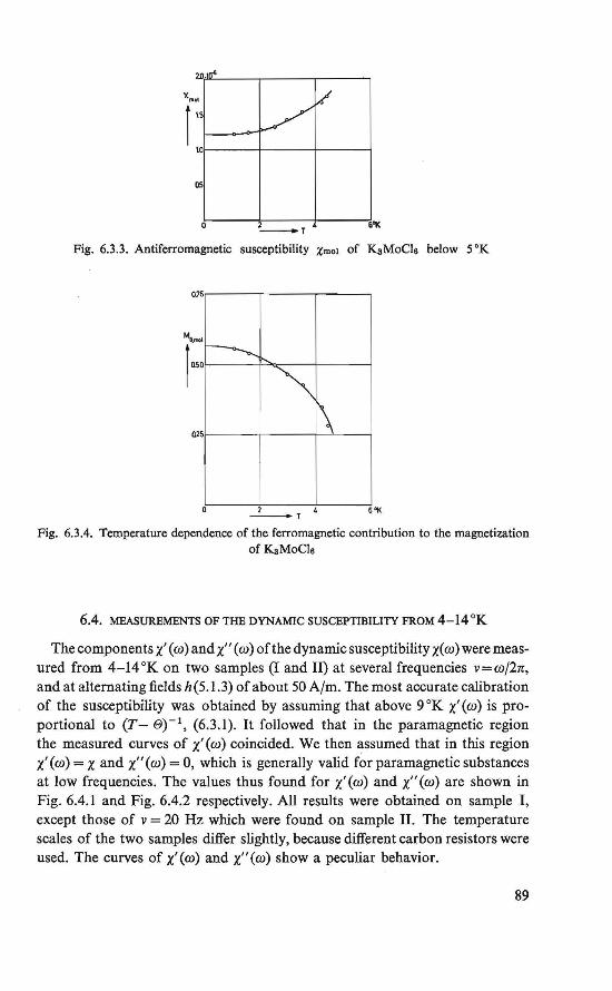
îl.S~ tOt----+----+-----i
os
~r' 6"K
Fig. 6.3.3. Antiferromagnetic susceptibility Xmo1 of KsMoCls below 5 °K
2 -r
6'1<
Fig. 6.3.4. Temperature dependence of the ferromagnetic contribution to the magnetization ofKaMoCls
6.4. MEASUREMENTS OF THE DYNAMIC SUSCEPTIBILITY FROM 4-14 °K
The components x' ( w) and x" ( w) of the dynamic susceptibility xC w) were measured from 4-14 °K on two samples (I and ID at several frequencies v=w/2n, and at alternating fields h(5. l.3) of about 50 A/m. The most accurate calibration of the susceptibility was obtained by assuming that above 9 °K x' (w) is proportional to (T- e)- 1
, (6.3.1). It followed that in the paramagnetic region the measured curves of x' ( w) coincided. We then assumed that in this region x' ( w) = x and x" ( w) = 0, which is generally valid for paramagnetic substances at low frequencies. The values thus found for x'(w) and x"(w) are shown in Fig. 6.4. l and Fig. 6.4.2 respectively. All results were obtained on sample I, except those of v = 20 Hz which were found on sample II. The temperature scales of the two samples differ slightly, because different carbon resistors were used. The curves of x'(w) and x"(w) show a peculiar behavior.
89
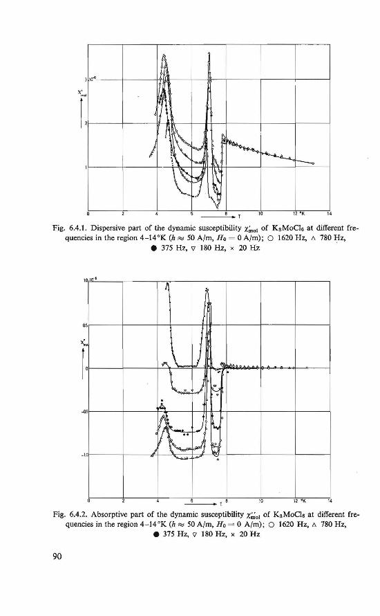
Fig. 6.4.1. Dispersive part of the dynamic susceptibility x;,,01 of K3 MoC16 at different frequencies in the region 4-l4°K (h""' 50 A/m, Ho= 0 A/m); O 1620 Hz, 1:; 780 Hz,
e 375 Hz, 'V 180 Hz, x 20 Hz
10 ,.,.,
~ L
05
x:. ~l ["
j j -"••.
L "' . ~
J ..j . ~
.QS
·~~-· b
..J \._
.J 5 .1.0
~ \-.--- - -;.
---•T 8 10 12 "K 14
Fig. 6.4.2. Absorptive part of the dynamic susceptibility x;,;01 of KaMoCls at different frequencies in the region 4-l4 °K (h""' 50 A/m, Ho= 0 A/m); O 1620 Hz, 1:; 780 Hz,
e 375 Hz, '\/ 180 Hz, x 20 Hz
90
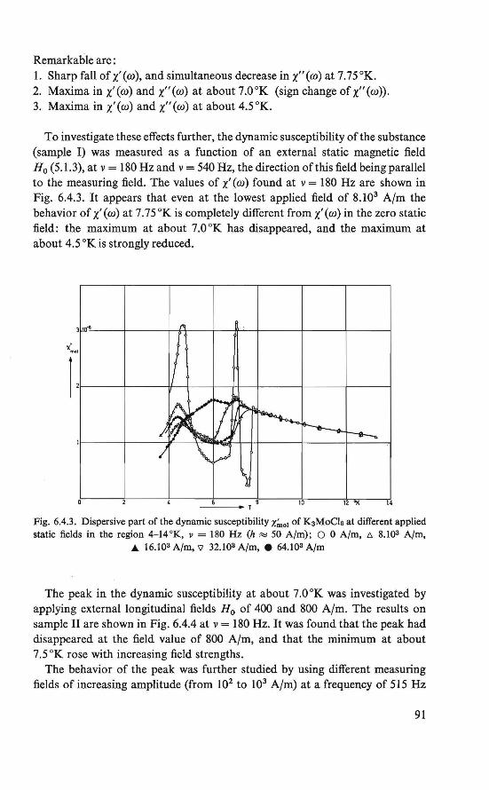
Remarkable are: l. Sharp fall of x' ( w ), and simultaneous decrease in x" ( w) at 7. 7 5 °K. 2. Maxima in x'(w) and x"(w) at about 7.0 °K (sign change ofx"(w)). 3. Maxima in x'(w) and x"(w) at about 4.5 °K.
To investigate these effects further, the dynamic susceptibility of the substance (sample 1) was measured as a function of an external statie magnetic field H0 (5.1.3), atv= 180 Hz and v = 540 Hz, the direction ofthis field being parallel to the measuring field. The values of x'(w) found atv= 180 Hz are shown in Fig. 6.4.3. lt appears that even at the lowest applied field of 8.103 A/m the behavior of x' (w) at 7.75 °K is completely different from x' (w) in the zero statie field: the maximum at about 7.0 °K bas disappeared, and the maximum at about 4.5 °K is strongly reduced.
10 12 'K
Fig. 6.4.3. Dispersive part of the dynamic susceptibility x;,,01 of K3MoCl6 at different applied statie fields in the region 4-14 °K, v = 180 Hz (h,,,; 50 A/m); O 0 A/m, e:. 8.103 A/m,
A. 16.103 A/m, 'il 32.103 A/m, e 64.103 A/m
The peak in the dynamic susceptibility at about 7.0 °K was investigated by applying external longitudinal fields H 0 of 400 and 800 A/m. The results on sample II are shown in Fig. 6.4.4 at v = 180 Hz. lt was found that the peak had disappeared at the field value of 800 A/m, and that the minimum at about 7.5 °K rose with increasing field strengths.
The behavior of the peak was further studied by using different measuring fields of increasing amplitude (from 102 to 103 A/m) at a frequency of 515 Hz
91
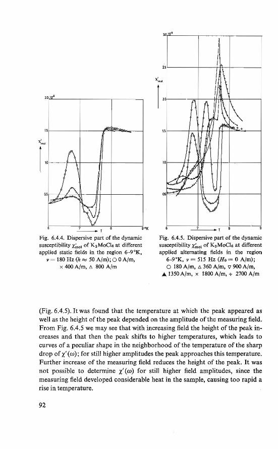
20~----,---------.------,
1.sl----+-----1'!-~~i......~---I
x' mol
Fig. 6.4.4. Dispersive part of the dynamic susceptibility x;,,01 of KsMoCl6 at different applied statie fields in the region 6-9 °K,
v = 180 Hz (h F:::i 50 A/m); O 0 A/m, x 400 A/m, t:. 800 A/m
10 •
Fig. 6.4.5. Dispersive part of the dynamic susceptibility x;,,01 of KsMoCfo at different applied alternating fields in the region
6-9°K, v = 515 Hz (Ho= 0 A/m); O 180 A/m, t:. 360 A/m, \/ 900 A/m,
À 1350 A/m, x 1800 A/m, + 2700 A/m
(Fig. 6.4.5). It was found that the temperature at which the peak appeared as well as the height of the peak depended on the amplitude of the measuring field. From Fig. 6.4.5 we may see that with increasing field the height of the peak increases and that then the peak shifts to higher temperatures, which leads to curves of a peculiar shape in the neighborhood of the temperature of the sharp drop of x' ( w); for still higher amplitudes the peak approaches this temperature. Further increase of the measuring field reduces the height of the peak. lt was not possible to determine x' (w) for still higher field amplitudes, since the measuring field developed considerable heat in the sample, causing too rapid a rise in temperature.
92
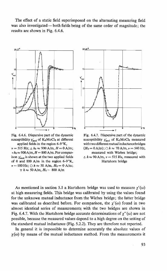
The effect of a statie field superimposed on the alternating measuring field was also investigated- both fields being of the same order of magnitude; the results are shown in Fig. 6.4.6.
20 •
-r
Fig. 6.4.6. Dispersive part of the dynamic susceptibility x;,,01 of KaMoC16 at different
applied fields in the region 6--9°K, v = 515 Hz; 6 ho~ 900 A/m, H = 0 A/m; x ho~ 900 A/m, H = 800 A/m. For comparison x;,,ol is shown at the two applied fields of 0 and 800 A/m in the region 6--9 °K, v = 180Hz; Oh~ 50 A/m, Ho= 0 A/m;
'V h ~ 50 A/m, Ho= 800 A/m
2.0 ·•
1.se------l-------4----I-....:.:::::~,.,_~
9 'K
Fig. 6.4.7. Dispersive part of the dynamic susceptibility x;,,01 of KaMoC16 measured with two different mutual inductancebridges (Ho= OA/m); 0 h ~ 70 A/m, v = 540 Hz,
measured with Wiebes bridge; 6 h ~ 90 A/m, v = 515 Hz, measured with
Hartshorn bridge
As mentioned in section 5.1 a Hartshorn bridge was used to measure x'(w) at high measuring fields. This bridge was calibrated by using the values found for the unknown mutual inductance from the Wie bes bridge; the latter bridge was calibrated as described before. For comparison, the x' (w) found in two almost identical series of measurement~ with the two bridges are shown in Fig. 6.4.7. With the Hartshorn bridge accurate determinations of x" (w) are not possible, because the measured values depend to a high degree on the setting of the standard mutual inductance (Fig. 5.2.2). They are therefore not reported.
In general it is impossible to determine accurately the absolute values of x(w) by means of the mutual inductance method. From the measurements it
93
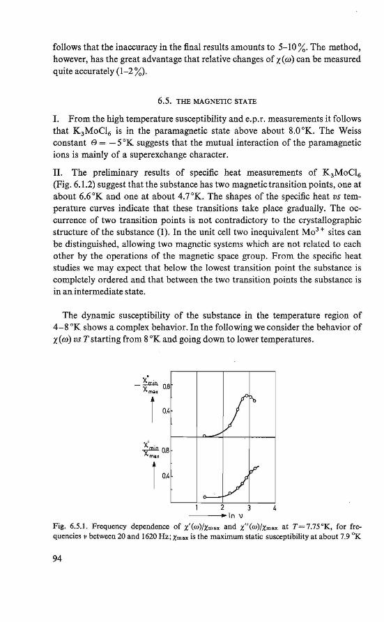
follows that the inaccuracy in the final results amounts to 5-10%. The method, however, has the great advantage that relative changes of x(w) can be measured quite accurately (1-2 %).
6.5. THE MAGNETIC STATE
I. From the high temperature susceptibility and e.p. r. measurements it follows that K 3 MoCl6 is in the paramagnetic state above about 8.0°K. The Weiss constant e = - 5 °K suggests that the mutual interaction of the paramagnetic ions is mainly of a superexchange character.
II. The prelim.inary results of specific heat m:easurements of K 3 MoCl6
(Fig. 6.1.2) suggest that the substance has two magnetic transition points, one at about 6.6°K and one at about 4.7°K. The shapes of the specific heat vs temperature curves indicate that these transitions take place gradually. The occurrence of two transition points is not contradictory to the crystallographic structure of the substance (1). In the unit cell two inequivalent Mo3 + sites can be distinguished, allowing two magnetic systems which are not related to each other by the operations of the magnetic space group. From the specific heat studies we may expect that below the lowest transition point the substance is completely ordered and that between the two transition points the substance is in an intermediate state.
The dynam.ic susceptibility of the substance in the temperature region of 4-8 °K shows a complex behavior. In the following we consider the behavior of x(w) VS Tstarting from 8 °K and going down to lower temperatures.
x· . -= 0.8 Xmor
x' . ~0.8
"'"'
1 OA
---•ln \1
Fig. 6.5.l. Frequency dependence of x'(w)/Xmax and x"(w)/Xma.x at T=7.75°K, for fr~ quencies v between 20 and 1620 Hz; Xma.x is the maximum statie susceptibility at about 7.9 °K
94
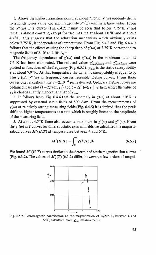
l. Above the highest transition point, at about 7.75°K, x' (w) suddenly drops to a much lower value and simultaneously x" ( w) reaches a large value. From the x"(w) vs T curves (Fig. 6.4.2) it may be seen that below 7.75 °K x"(w) remains almost constant, except for two maxima at about 7.0 °K and at about 4.7 °K. This suggests that the relaxation mechanism which obviously exists below 7.75°K, is independent of temperature. From Fig. 6.4.3 and Fig. 6.4.4 it follows that the effects causing the sharp drop of x' (w) at 7. 75 °K correspond to magnetic fields of 2.103 to 4.103 A/m.
The frequency dependence of x'(w) and x"(w) in the minimum at about 7.6°K has been elaborated. The reduced values X~;n/xmax and X'.:i;n/Xmax were plotted as functions of the frequency (Fig. 6.5.1) ; Xmax is the statie susceptibility x at about 7.9°K. At that temperature the dynamic susceptibility is equal to X· The x'(w), x"(w) vs frequency curves resemble Debije curves. From these curves one relaxation timer =2.10- 4 sec is derived. Ordinary Debije curves are obtained if we plot {1-2x' (w)/xd and { -2x" (w)/xi} vs lnw, where the value of X 1 is cbosen slightly higher than that of Xmax.
2. It follows from Fig. 6.4.4 tbat the anomaly in x(w) at about 7.0 °K is suppressed by external statie fields of 800 A/m. From the measurements of x(w) at relatively strong measuring fields (Fig. 6.4.5) it is derived that the peak shifts to higher temperatures at a rate whicb is roughly Iinear to the amplitude of the measuring field.
3. At about 4.5 °K there also occurs a maximum in x'(w) and x"(w). From the x' (w) vs Tcurves for different statie external fields we calculated the magnetization curves M'(H,T) at temperatures between 4 and 5°K.
M'(H, T) = LH x'(h, T)dh (6.5.1)
We found M' (H, T) curves similar to the determined statie magnetization curves (Fig. 6.3.2). The values of M~(T) (6.3.2) differ, however, a few orders of magni-
0.01 2
1 }\ M:...
) a~ .i' 1
M04
6"K ---+T
Fig. 6.5.2. Ferromagnetic contribution to the magnetization of K3MoCls between 4 and 5 °K, calculated from x;,,01 measurements
95
tude from the statie values (Fig. 6.3.4, Fig. 6.5.2). It may be seen from Fig. 6.3.4 and Fig. 6.5.2 that both M 0 andM~ become zero at about 5.0°K. If we compare Fig. 6.3.3 and Fig. 6.4.3 we note that below 4 °K x' (ro) tends to values below the statie susceptibility. The Iowering of M 0 (T) and x'(ro) compared with the statie values is presumably caused by the relaxation mechanism which obviously exists in this temperature region.
UI. In the liquid 4 He temperature region the substance is probably in an antiferromagnetic state, in which the electron spins are not exactly antiparallel but slightly canted, giving rise to a weak parasitic ferromagnetism. This follows from the statie magnetization measurements (Fig. 6.3.3, Fig. 6.3.4). The curves show that the substance has a rather normal magnetic behavior in the liquid 4 He temperature regioti (14). Extrapolation of the curve of Fig. 6.3.4 shows that the ferromagnetic component disappears at about 5.0 °K. At 0 °K the saturation value of the calculated average ferromagnetic component per Mo3 + ion is about 0.1 Bohr magneton.
It is noted here that such a canted antiferromagnetic structure is allowed by the crystallographic space group (compare sections 7.4 and 8.4).
The behavior of x' (ro) and x" (ro) at temperatures below 4 °K has not been investigated. However, it is clear that the dynamic susceptibility vs temperature shows a maximum at about 4.5 °K, and that the curves of both x vs T and x' (ro) vs T (Fig. 6.3.3, Fig. 6.4.1) at liquid 4 He temperatures decrease with decreasing temperature.
It should be noted that prelirninary measurements on the magnetic ordering of K3 MoC16 by means of neutron diffraction (1) revealed an onset of magnetic ordering at 4.2 °K and a completely ordered state at about 1.5 °K.
6.6. DISCUSSION OF THE INTERMEDIATE STATE
The salt K3 MoCl6 shows an unusual magnetic behavior between 4 and 8 °K. With due reserve we propose the following explanation of the observed phenomena:
From the structure analysis (6.1) it followed that in the crystallographic structure of K3 MoCJ6 two inequivalent Mo3 + sites can be distinguished. In the paramagnetic region the exchange interactions between the Mo3 + ions of one set differ from those between the Mo3 + ions of the two sets.
The specific heat studies suggest that one set of ions (system A) orders at about 6.6 °K and the other (system B) remains paramagnetic. The hightemperature expansion of the susceptibility ( e < 0) suggests that system A orders antiferromagnetically. In crystal structures of such a low symmetry this will be generally a canted antiferromagnetic structure.
The drop in x(ro) at 7.75°K can be understood when x(ro) is the difference of
96
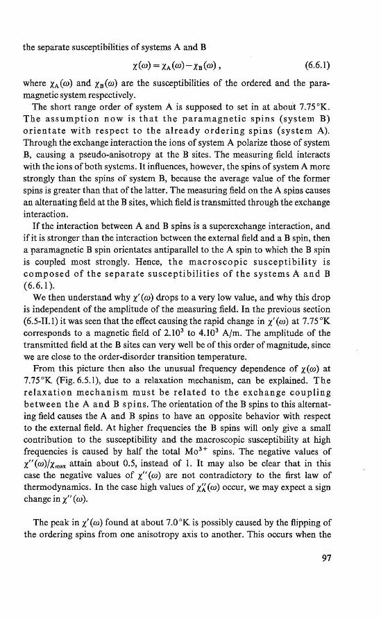
the separate susceptibilities of systems A and B
x(w) = XA(w)-xu(w)' (6.6.I)
where XA(w) and xu(w) are the susceptibilities of the ordered and the paramagnetic system respectively.
The short range order of system A is supposed to set in at about 7.75°K. The assumption now is that the paramagnetic spins (system B) orientate with respect to the already ordering spins (system A). Through the exchange interaction the ions of system A polarize those of system B, causing a pseudo-anisotropy at the B sites. The measuring field interacts with the ions ofboth systems. It influences, however, the spins of system Amore strongly than the spins of system B, because the average value of the former spins is greater than that of the latter. The measuring field on the A spins causes an a:lternating field at the B sites, which field is transmitted through the exchange interaction.
If the interaction between A and B spins is a superexchange interaction, and if it is stronger than the interaction between the external field and a B spin, then a paramagnetic B spin orientates antiparallel to the A spin to which the B spin is coupled most strongly. Hence, the macroscopie susceptibility is composed of the separate susceptibilities of the systems A and B (6.6.1).
We then understand why x'(w) drops toa very low value, and why this drop is independent of the amplitude of the measuring field. In the previous section (6.5-II.l) it was seen that the effect causing the rapid change in x' (w) at 7.75 °K corresponds to a magnetic field of 2.103 to 4.103 A/m. The amplitude of the transmitted field at the B sites can very well be of this order of magnitude, since we are close to the order-disorder transition temperature.
From this picture then also the unusual frequency dependence of x(w) at 7.75°K (Fig. 6.5.1), due to a relaxation mechanism, can be explained. The relaxation mechanism must be related to the exchange coupling between the A and B spins. The orientation of the B spins to this alternating field causes the A and B spins to have an opposite behavior with respect to the external field. At higher frequencies the B spins wil! only give a small contribution to the susceptibility and the macroscopie susceptibility at high frequencies is caused by half the total Mo3 + spins. The negative values of x" (w)/Xmax attain about 0.5, instead of 1. It may also be clear that in this case the negative values of x" ( w) are not contradictory to the first law of thermodynamics. In the case high values of x~ (w) occur, we may expect a sign change in x" ( w ).
The peak in x'(w) found at about 7.0°K is possibly caused by the flipping of the ordering spins from one anisotropy axis to another. This occurs when the
97
coupling of the spins-with average magnetic moment (µ)-to the measuring field becomes strong enough to overcome the potential barrier. lt may then be expected in this picture that with increasing amplitude of the measuring field the anomaly will shift to higher temperatures, implying a lower value of(µ), until the value of (µ) becomes negligibly small. Since the effect causing the anomaly corresponds to only 400 to 800 A/m, the anisotropy energy of the spins is supposed to be small compared with the coupling to a statie. field higher than, for instance, 103 A/m, and the peak will vanish, as it did in our experiments.
The maximum in x'(w) at about 4.5 °K can be ascribed to the onset of magnetic ordering of the paramagnetic system. As was derived from the statie magnetization measurements, the substance in the complete!y ordered state has a weak ferromagnetic component. This component, then, can give rise to a peak in x' (w); see also ref. 14.
Finally it is noted that in a few other substances, too, a somewhat similar magnetic behavior seems to occur. For instance, the salt Ni(I03) 2 .2H20 (15, 16, 17) shows two distinguishable peaks in the specific heat vs temperature curve, and antiferromagnetic ordering accompanied by a weak ferromagnetism at temperatures below the lowest specific heat maximum. The substances Ul3
(18), and CeCl3 , PrC13 , NdCl 3 (19) show anomalies in x'(w) vs Tof the type which we found at 7.0 °K.
These measurements, however, are too incomplete to allow of a detailed comparison, and it would be interesting to investigate these substances more rigorously, in order to check or modify the model which has been proposed by US.
REFERENCES
1. B. van Laar, R. C. N., Petten, The Netherlands, private communication. 2. B. Th. Tjabbes, Proc. Kon. Akad. Wetenschappen, 35 (1932) 693. 3. C. Epstein and N. Elliott, J. Chem. Phys., 22 (1954) 634. 4. J. H.E. Griffiths, J. Owen and I.M. Ward, Proc. Roy. Soc., Lorulon, A219 (1953) 526. 5. J . S. Griffith, The Theory of Transition-Metal /ons, Cambridge Univ. Press, London and
New York (1961). 6. H. Hartmann and H. J. Schmidt, Z . Physik. Chemie neue Fo/ge, 11(1957)234. 7. A. Herweijer, /nternal Report, Low Temperature Group, Technologica! University,
Eindhoven (1966). 8. P. A. van Dalen, H. M. G ijsman, N. Love and H. Forstat, Proc. /Xth Low Tempera/ure
Co11fere11ee, Columbus, Ohio (1964) 888. 9. J . H . Van Vleck, The Theory of Eleciric and Magnetic Susceptibilities, Oxford Univ. Press,
London (1932). 10. C. Domb and A. R. Miedema, Progress in Low Temperature Physics IV, p. 296 (C. J .
Gorter, ed.), North-Holland Publishing Company, Amsterdam (1964). 11. C. J. Gorter, Paramagnetic Re/axation, Elsevier Publishing Company, Amsterdam (1947). 12. C. J . Gorter, Progress ifi Low Temperature Physics II, p. 266 (C. J. Gorter, ed.), North
Holland Publishing Company, Amsterdam (1957).
98
13. H. M. Rosenberg, Low Tempera/ure Solid State Physics, Oxford Univ. Press, London (1963).
14. T. Moriya, Magnetism /, p. 85 (G. T. Rado and H. Suhl, eds.), Academie Press, New York and London (1963).
15. J.C. Burgiel, V. Jaccarino and A. L. Schawlow, Phys. Rev., 122 (1961) 429. 16. F. J. du Chatenier, B. M. Boerstoel and J. de Nobel, Physica, 30(1964)1625. 17. H.C. Meyer and J. van den Handel,Physica, 30 (1964) 1633. 18. L. D. Roberts and R. B. Murray, Phys. Rev., 100 (1955) 650. 19. J.C. Eisenstein, R. P. Hudson and B. W. Mangum, Phys. Rev., 137 (1965) A1886.
99
7. PROTON RESONANCE STUDY OF THE MAGNETIC STATE OF
FeCl2.4H2 0 BELOW 4.2 °K *)
This chapter describes the investigation of the ordered magnetic state in FeC12.4H20 by proton resonance. The proton resonance of FeCb.4H20 has been examined in the temperature range of 0.35 °K to 4.2 °K. In the region of 1.1 °K to 4.2 °K a proton resonance pattern was found, characteristic of the paramagnetic state, and below 0. 7 °K, lines were observed characteristic of the antiferromagnetic state. In the intermediate temperature range no proton resonance absorption could be detected. By combining the crystallographic symmetry and the symmetry of the local fields at the proton sites, a structure of the antiferromagnetic spin arrangement is proposed.
7.1. INTRODUCTION
The crystal structure of FeC12 .4H20 has been determined by Penfold and Grigor (1). The space group is P2ifc and there are two formula units in the chemical unit cell. The Fe2 + ions occupy inversion centers at the corners and the centers of the b, c-faces of the cell. Each magnetic ion is surrounded by four 0 2
- ions and two ei- ions in a distorted octahedral arrangement (local point symmetry 2/m). El Saffar and Murty, by studying proton resonance at room temperature, showed that the point symmetry of the hydrogen positions is also 2/m (2).
An onset of a specific heat anomaly in FeC12 .4H20 at approximately 1.1 °K was reported by Friedberg, Cohen and Schelling (3). Schriempf and Friedberg (4) reported that the susceptibility of FeC12 .4H20between 1.1°Kand4.2°Kis highly anisotropic with X~ > x:· > X~· Above 1.25 °K, X~ and x:· increase slowly with decreasing temperature, while x~ remains constant. Below 1.1 °K, x~ and x:· decrease rapidly and at approximately 0.7°K they become equal. Below 0.7°K, x:· and x~ remain equal to each other and are nearly temperature independent, and x~ decreases rapidly with decreasing temperature. These susceptibility data indicate a rather nonna! antiferromagnetic behavior of FeCl2 .4H20 below 0.7°K.
7 .2. THE EXPERIMENT
The temperature range between 0.35°K and l.5°K was achieved with a small glass 3 He cryostat (5). The coil of the marginal oscillator was wound on the outside of the vacuumjacket surrounding the 3 He and the crystal. Temperatures were determined by measuring the 3He vapor pressure and applying thermo-
•) This work was supported by the U.S. Air Force Office of Scientific Research.
100
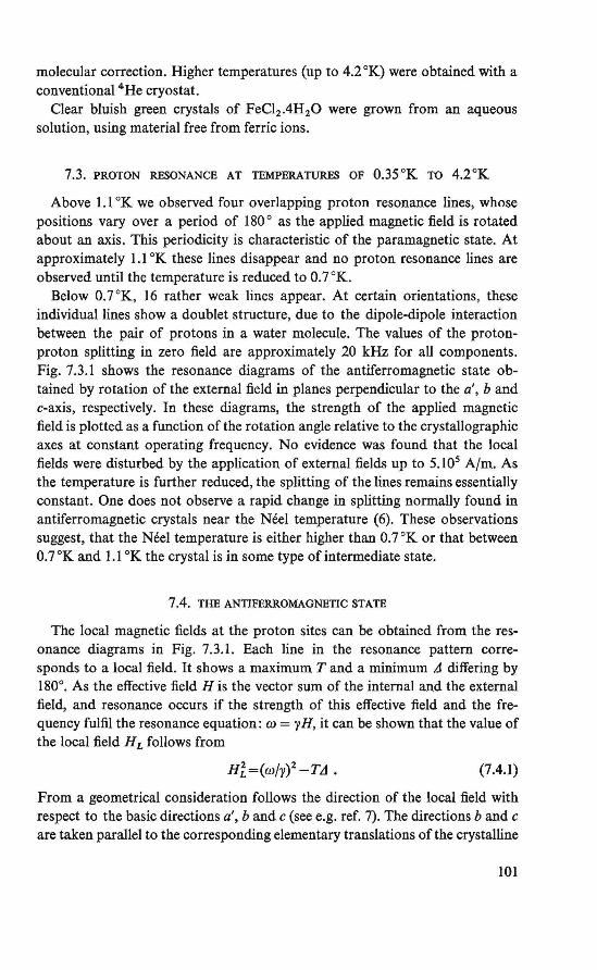
molecular correction. Higher temperatures (up to 4.2 °K) were obtained with a conventional 4 He cryostat.
Clear bluish green crystals of FeC12 .4H20 were grown from an aqueous solution, using material free from ferric ions.
7.3. PROTON RESONANCE AT TEMPERATURES OF 0.35°K TO 4.2°K
Above 1.1 °K we observed four overlapping proton resonance lines, whose positions vary over a period of 180 ° as the applied magnetic field is rotated about an axis. This periodicity is characteristic of the paramagnetic state. At approximately 1.1 °K these lines disappear and no proton resonance lines are observed until the temperature is reduced to 0.7°K.
Below 0.7°K, 16 rather weak lines appear. At certain orientations, these individual lines show a doublet structure, due to the dipole-dipole interaction between the pair of protons in a water molecule. The values of the protonproton splitting in zero field are approximately 20 kHz for all components. Fig. 7.3. l shows the resonance diagrams of the antiferromagnetic state obtained by rotation of the external field in planes perpendicular to the a', b and c-axis, respectively. In these diagrams, the strength of the applied magnetic field is plotted as a function of the rotation angle relative to the crystallographic axes at constant operating frequency. No evidence was found that the local fields were disturbed by the application of external fields up to 5.105 A/m. As the temperature is further reduced, the splitting of the Iines remains essentially constant. One does not observe a rapid change in splitting normally found in antiferromagnetic crystals near the Néel temperature (6). These observations suggest, that the Néel temperature is either higher than 0.7°K or that between 0.7°K and 1.1 °K the crystal is in some type ofintermediate state.
7.4. THE ANTIFERROMAGNETIC STATE
The local magnetic fields at the proton sites can be obtained from the resonance diagrams in Fig. 7.3.1. Each line in the resonance pattern corresponds to a local field. It shqws a maximum T and a minimum LI differing by 180°. As the effective field H is the vector sum of the internal and the external field, and resonance occurs if the strength of this effective field and the frequency fulfil the resonance equation: w = yH, it can be shown that the value of the local field HL follows from
(7.4.1)
From a geometrical consideration follows the direction of the local field with respect to the basic directions a', band c (see e.g. ref. 7). The directions band c are taken parallel to the corresponding elementary translations of the crystalline
101
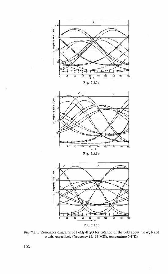
,,10'
Ê ~
u ·z t r,
20 40 60 80 100 120 140 160 180
' Fig. 7.3.la
a·
i ~ 'O
~ 3.10'!> u
c g 2.10'
j ,.. 20 40 1 0 _,
Fig. 7.3.lb
·~
f
r:l~o' ~~ Fig. 7.3.lc
Fig. 7.3.1. Resonance diagrams of FeCl2.4H20 for rotation of the field about the a', band c-axis respectively (frequency 12.155 MHz, temperature 0.4 °K)
102
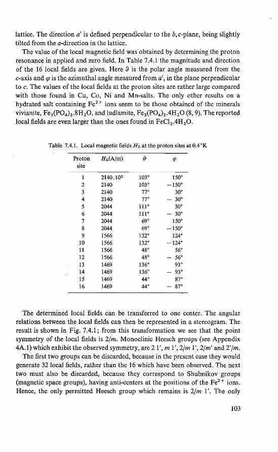
lattice. The direction a' is defined perpendicular to the b, c-plane, being slightly tilted from the a-direction in the lattice.
The value of the local magnetic field was obtained by determining the proton resonance in applied and zero field. In Table 7.4.1 the magnitude and direction of the 16 local fields are given. Here 8 is the polar angle measured from the c-axis and q> is the azimuthal angle measured from a', in the plane perpendicular to c. The values of the Jocal fields at the proton sites are rather large compared with those found in Cu, Co, Ni and Mn-salts. The onJy other results on a hydrated salt containing Fe2+ ions seem to be those obtained of the minerals vivianite, Fe3(P04 )i.8H20, and ludlamite, Fe3(P04 ) 2 .4H20 (8, 9). The reported local fields are even larger than the ones found in FeCl2 .4H20.
Table 7.4.1. Local magnetic fields HL at the proton sites at 0.4 °K
Proton HL(A/m) {} <p
site
2140.102 103° 150° 2 2140 103° -150° 3 2140 77° 30° 4 2140 770 - 30° 5 2044 111° 30° 6 2044 111° - 30° 7 2044 69° 150° 8 2044 69° -150° 9 1566 132° 124°
10 1566 132° -124° 11 1566 480 56° 12 1566 48° - 56° 13 1469 136° 93° 14 1469 136° 93° 15 1469 440 870
16 1469 440 87°
The determined Jocal fields can be transferred to one center. The anguJar relations between the local fields can then be represented in a stereogram. The result is shown in Fig. 7.4. l ; from this transformation we see that the point symmetry of the local fields is 2/m. Monoclinic Heesch grollps (see Appendix 4A.1) which exhibit the observed symmetry, are2 l', m I', 2/m l', 2/m' and 2'/m.
The first two groups can be discarded, because in the present case they would generate 32 local fields, rather than the 16 which have been observed. The next two must also be discarded, because they correspond to Shubnikov groups (magnetic space groups), having anti-centers at the positions of the Fe2 + ions. Hence, the only permitted Heesch group which remains is 2/m l'. The only
103
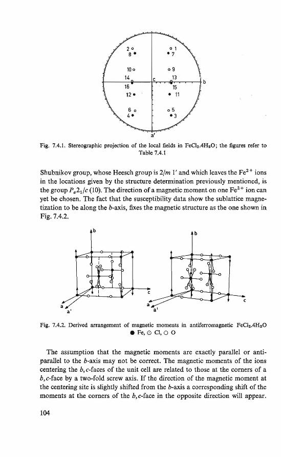
100 0 9
14 c 13 -i--~~----1t--~-r,.....,---r->trr--.-,....-,.----(-b
16 15
12. • 11
a'
Fig. 7.4.1. Stereographic projection of the local fields in FeCl2.4H20; the figures refer to Table 7.4.1
Shubnikov group, whose Heesch group is 2/m 1' and which leaves the Fe2 + ions in the locations given by the structure determination previously mentioned, is the group Pa2ifc (10). The direction of a magnetic moment on one Fe2 + ion can yet be chosen. The fact that the susceptibility data show the sublattice magnetization to be along the b-axis, fixes the magnetic structure as the one shown in Fig. 7.4.2.
b b
c
Fig. 7.4.2. Derived arrangement of magnetic moments in antiferromagnetic FeCl2.4H20 e Fe,O Cl, 0 0
The assumption that the magnetic moments are exactly parallel or antiparallel to the b-axis may not be correct. The magnetic moments of the ions centering the b, c-faces of the unit cel! are related to those at the corners of a b, c-face by a two-fold screw axis. If the direction of the magnetic moment at the centering site is slightly shifted from the b-axis a corresponding shift of the moments at the corners of the b,c-face in the opposite direction will appear.
104
7.5. CONCLUSION
Using the observed local fields and symmetry arguments a structure of the antiferromagnetic moments can be proposed. The susceptibility data also indicate normal antiferromagnetic behavior of FeCl2 .4H20 below 0.7°K. This is comprehensible, if we assume that the exchange mechanism between two Fe2 + ions via the chlorine ions is mainly of a superexchange character, and that via the water molecules ofhydration, it is mainly direct (chapter 3). We can very well imagine that in a crystal structure with the low symmetry P2ifa, a canting of the atomie magnetic moments is possible.
Since both the susceptibility and proton resonance leave the temperature range of0.7 to 1.1 °K as a region of ill-defined magnetic behavior, specific heat studies in this range would be most interesting. After the publication of the present work (11), Uryû (12) considered the ordered antiferromagnetic state of FeCl2 .4H20 from a theoretica! point of view. His result agrees with the proposed spin arrangement, in which the magnetic moments are slightly canted from the b-axis in the a-direction.
REFERENCES
1. B. R. Penfold and J. A. Grigor, Acta Cryst., 12 (1959) 850. 2. Z.H. El Saffar and C. R. K. Murty, Acta Cryst., 15 (1962) 285. 3. S. A. Friedberg, A. F. Cohen and J. H. Schelling, Proc. lrtt. Conference ort Magrtetism
and Crysta//ography, Kyoto, Japan, 1(1961)515. 4. J. T. Schriempf and S. A. Friedberg, Phys. Rev., 136 (1964) A518. 5. J. A. Cowen, R. D. Spence, H. Van Till and H. Weinstock, Rev. Sci. lnstr., 35 (1964) 914. 6. N. J. Poulis and G. E.G. Hardeman, Physica, 18 (1952) 201. 7. W. van der Lugt, Thesis, Leiden (1961). 8. W. van der Lugt and N. J. Poulis, Physica, 27 (1961) 733. 9. T. W. J. van Agt and N. J. Poulis, Physica, 30 (1964) 588.
10. E. P. Riedel and R. D. Spence, Physica, 26 (1960) 1174. 11. R. D. Spence, R. Au and P.A. van Dalen, Physica, 30 (1964) 1612. 12. N. Uryii, Phys. Rev., 136 (1964) A527.
105
8. PROTON RESONANCE STUDY OF THE MAGNETIC STATE OF
Cu(COOH)2.4H20 AND Cu(COOH)2.4020 AT 4.2 °K
The magnetic state of Cu(COOH)2.4H20 and Cu(COOH)2.4D20 at 4.2 °K has been investîgated by studying the proton resonance. We found a resonance pattem which is characterîstîc of the antiferromagnetîc state. From these resonance results we could determîne a magnetîc point symmetry. Making use of this symmetry and the crystallograpbic space group, a magnetîc stmcture could be proposed.
8.1. INTRODUCTION
The results of the paramagnetic susceptibility measurements of Martin and Waterman (1) on powdered Cu(COOH)i.4H20 from 80°K to 360°K showed a large Weiss constant of -175 °K indicating a strong exchange interaction between the Cu2 + ions. Haseda et al. (2) and Flippen et al. (3) studied the susceptibility of this substance on single crystals below 80°K. They found a broad weak maximum at 17 °K in two crystallographic directions. Proton resonance studies were reported by ltoh and Kamiya ( 4); they mention that the crystal is in the antiferromagnetic state below 17 °K. Magnetization and susceptibility measurements are also reported by Kobayashi and Haseda (5). They summarize their results as follows: "a broad maximum of the susceptibility at about 60 °K, a sharp transition to the antiferromagnetic state with parasitic ferromagnetism at 17.0°K and curious change of the magnetization with magnetic field at liquid helium temperatures".
The crystal structure of this material has been determined by Kiriyama et al. (6). They found the space groupP2 1/a, with two formula units in the unit cell. Remarkable for this structure is a definite layer structure. Four oxygen ions, belonging to different formate molecules surround a Cu2+ ion in a square planar configuration. These planes of copper formate were separated from each other by the water molecules of hydration. The hydrogen positions in this structure are studied by Kiriyama (7) by looking at the proton-proton interaction in a water molecules in the crystal with n.m. r. These positions are recently determined with a neutron diffraction study of this substance (8).
The purpose of the present study is the investigation of the magnetic ordering in Cu(COOH)i.4H20 below l7°K. The proton resonance spectra which were found in this temperature range, were very complicated. For this reason the H 20 molecules were replaced by molecules D 20. The nuclear resonance of the protons in the formate group was then investigated.
106
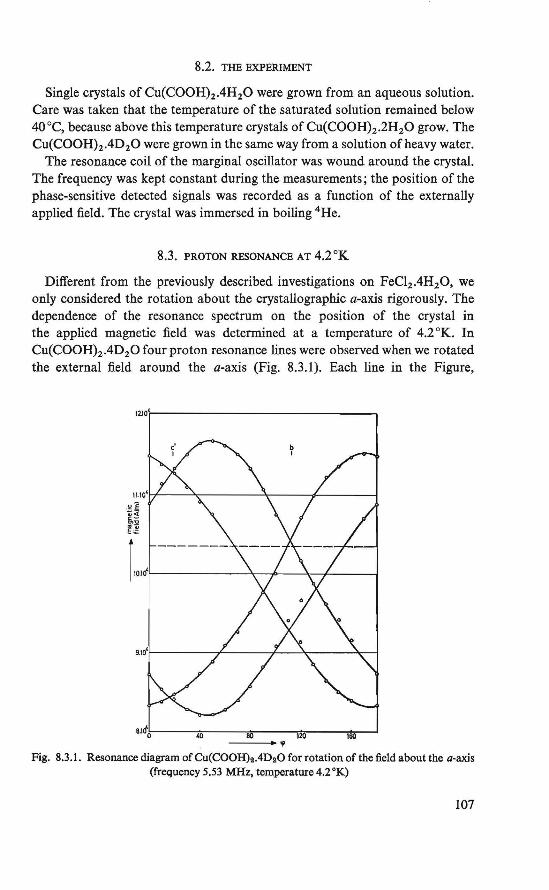
8.2. THE EXPERIMENT
Single crystals of Cu(COOH)i.4H20 were grown from an aqueous solution. Care was taken that the temperature of the saturated solution remained below 40 °C, because above this temperature crystals of Cu(COOH)i.2H20 grow. The Cu(COOH)i.4D20 were grown in the same way from a solution of heavy water.
The resonance coil of the marginal oscillator was wound around the crystal. The frequency was kept constant during the measurements; the position of the phase-sensitive detected signals was recorded as a function of the externally applied field. The crystal was immersed in boiling 4 He.
8.3. PROTON RESONANCE AT 4.2 °K
Different from the previously described investigations on FeCl2 .4H20, we only considered the rotation about the crystallographic a-axis rigorously. The dependence of the resonance spectrum on the position of the crystal in the applied magnetic field was determined at a temperature of 4.2 °K. In Cu(COOH)i.4D20 four proton resonance lines were observed when we rotated the external field around the a-axis (Fig. 8.3.1). Each line in the Figure,
12.104
b 1
11.10'
·~~ ~ -"'l3 Ë~
[",,
___ " Fig. 8.3.1. Resonance diagram of Cu(COOH)2.4D20 for rotation of the field about the a-axis
(frequency 5.53 MHz, temperature 4.2°K)
107
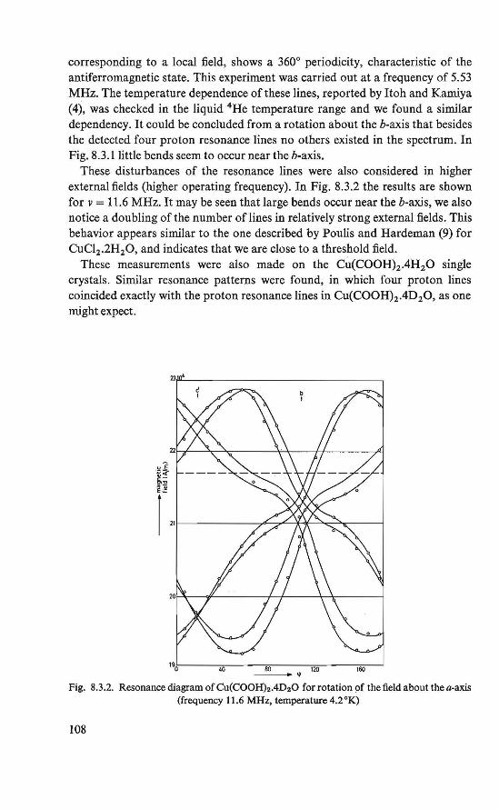
corresponding to a local field, shows a 360° periodicity, characteristic of the antiferromagnetic state. This experiment was carried out at a frequency of 5.53 MHz. The temperature dependence of these lines, reported by Itoh and Kamiya (4), was checked in the liquid 4 He temperature range and we found a similar dependency. It could be concluded from a rotation about the b-axis that besides the detected four proton resonance lines no others existed in the spectrum. In Fig. 8.3.1 little bends seem to occur near the b-axis.
These disturbances of the resonance lines were also considered in higher external fields (higher operating frequency). In Fig. 8.3.2 the results are shown for v = 11.6 MHz. It may be seen that large bends occur near the b-axis, we also notice a doubling of the number of lines in relatively strong extemal fields. This behavior appears similar to the one described by Poulis and Hardeman (9) for CuC12 .2H20, and indicates that we are close toa threshold field.
These measurements were also made on the Cu(COOH)i.4H20 single crystals. Similar resonance patterns were found, in which four proton lines coincided exactly with the proton resonance lines in Cu(COOH)2 .4D20, as one might ex peet.
g~ :!-"'" Ë~
r ",_______________....-------------
---.P
Fig. 8.3 .2. Resonance diagram of Cu(COOH)2.4D20 for rotation of the field about the a-axis (frequency 11.6 MHz, temperature 4.2 °K)
108
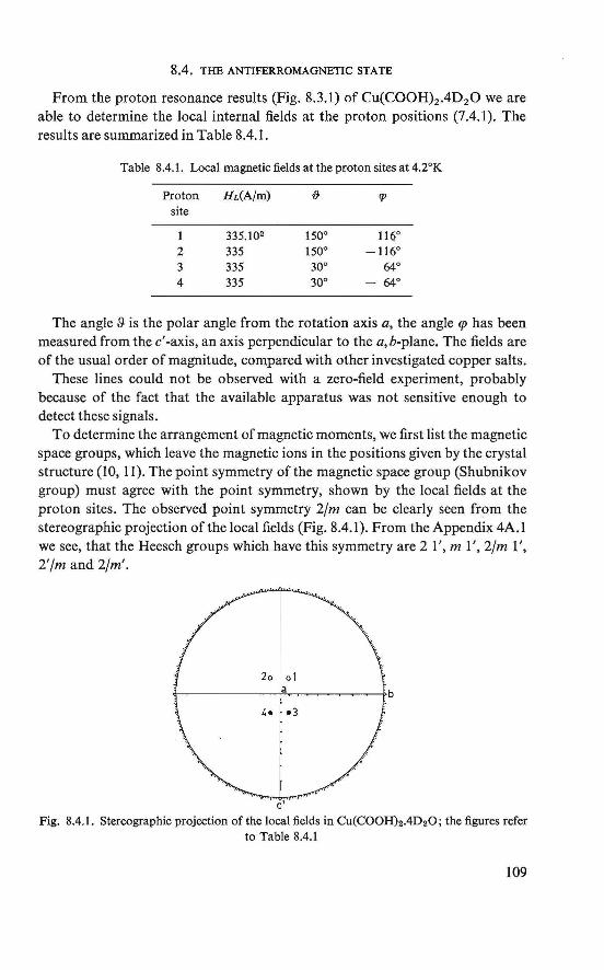
8.4. THE ANTIFERROMAGNETIC STATE
From the proton resonance results (Fig. 8.3.1) of Cu(COOH)i.4D2 0 we are able to determine the local internal fields at the proton positions (7.4.1). The results are summarized in Table 8.4.1.
Tab Ie 8.4.1. Local magnetic fields at the proton sites at 4.2°K
Proton HL(A/m) 1} rp site
1 335.102 150° 116° 2 335 150° -116° 3 335 30° 640
4 335 30° - 640
The angle 9 is the polar angle from the rotation axis a, the angle <p has been measured from the c' -axis, an axis perpendicular to the a, b-plane. The fields are of the usual order of magnitude, compared with other investigated copper salts.
These lines could not be observed with a zero-field experiment, probably because of the fact that the available apparatus was not sensitive enough to detect these signals.
To determine the arrangement of magnetic moments, we first list the magnetic space groups, which leave the magnetic ions in the positions given by the crystal structure (10, 11).The point symmetry of the magnetic space group (Shubnikov group) must agree with the point symmetry, shown by the local fields at the proton sites. The observed point symmetry 2/m can be clearly seen from the stereographic projection of the local fields (Fig. 8.4.1 ). From the Appendix 4A. l we see, that the Heesch groups which have this symmetry are 2 l', ml', 2/m l', 2'/m and 2/m'.
2o ol .,._~~~~~-t=a,,__..~~~~..---+b
4• •3
c' Fig. 8.4.1. Stereographic projection of the local fields in Cu(COOH)2.4D20; the figures refer
to Table 8.4.l
109
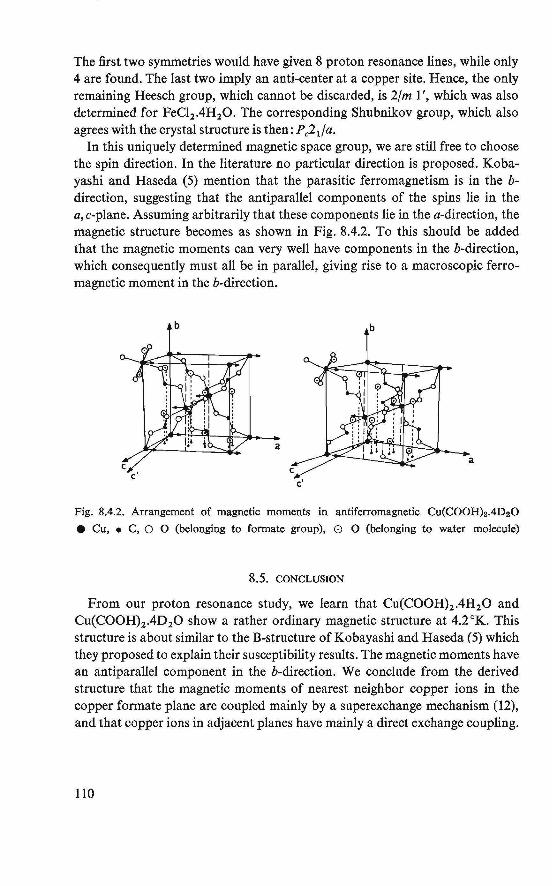
The first two symmetries would have given 8 proton resonance lines, while only 4 are found. The last two imply an anti-center at a copper site. Hence, the only remaining Heesch group, which cannot be discarded, is 2/m l', which was also determined for FeC12 .4H20. The corresponding Shubnikov group, which also agrees with the crystal structure is then: P ,,2 il a.
In this uniquely determined magnetic space group, we are still free to choose the spin direction. In the literature no particular direction is proposed. Kobayashi and Haseda (5) mention that the parasitic ferromagnetism is in the bdirection, suggesting that the antiparallel components of the spins lie in the a, c-plane. Assuming arbitrarily that these components lie in the a-direction, the magnetic structure becomes as shown in Fig. 8.4.2. To this should be added that the magnetic moments can very well have components in the b-direction, which consequently must all be in parallel, giving rise to a macroscopie ferromagnetic moment in the b-direction.
b b
a
Fig. 8.4.2. Arrangement of magnetic moments in antiferromagnetic Cu(COOH)2.4D20
e Cu, • C, O 0 (belonging to formate group), O 0 (belonging to water molecule)
8.5. CONCLUSION
From our proton resonance study, we learn that Cu(COOH)z.4H20 and Cu(COOH)z.4D20 show a rather ordinary magnetic structure at 4.2 °K. This structure is about similar to the B-structure of Kobayashi and Haseda (5) which they proposed to explain their susceptibility results. The magnetic moments have an antiparallel component in the b-direction. We conclude from the derived structure that the magnetic moments of nearest neighbor copper ions in the copper formate plane are coupled mainly by a superexchange mechanism (12), and that copper ions in adjacent planes have mainly a direct exchange coupling.
110
REFERENCES
1. R. L. Martin and H. Waterman, J. Chem. Soc. , (1959) 1359. 2. T. Haseda, A. R. Miedema, H . Kobayashi and E. Kanda, Proc. Int . Conference on
Magnetism and Crystallography, Kyoto, Japan, 1 (1961) 518. 3. R. B. Flippen and S. A. Friedberg, J. Chem. Phys., 38 (1963) 2652. 4. J. ltoh and Y. Kamiya, Proc. Int. Conference on Magnetism and Crystallography, Kyoto,
Japan, 1(1961)512. 5. H. Kobayashi and T. Haseda, J. Phys. Soc. Japan, 18 (1963) 541. 6. R. Kiriyama, H. Ibamoto and K. Matsuo, Acta Cryst" 1 (1954) 482. 7. H. Kiriyama, J. Chem. Soc. Japan, 35 (1962) 1205. 8. K. C. Turberfield, A.E. R. E., Harwell, U.K" private communication. 9. N. J. Poulis and G. E.G. Hardeman, Physica, 18 (1952) 315.
10. E. P. Riedel and R. D. Spence, Physica, 26 (1960) 1174. 11. E. P. Riedel, Ph.D. Thesis, Michigan State University (1 961). 12. A. Mookherji and S. C. Marthur, J. Phys. Chem. Solids, 24 (1963) 1386.
111
SAMENVATTING
In het eerste gedeelte van dit proefschrift wordt de statisch magnetisch geordende toestand van een antiferromagnetische stof - CuCl2 .2H20 - theoretisch onderzocht. Het tweede gedeelte bevat de resultaten van het experimentele onderzoek van de magnetische ordening van de isolatoren K 3MoC16 ,
FeC12 .4H20, Cu(COOH)i.4H2 0 en Cu(COOH)i.4D20. Hoofdstuk 1 geeft een algemene inleiding in het gebied van de magnetische
ordening en een overzicht van het werk, dat in deze dissertatie besproken wordt. In hoofdstuk 5 worden de toegepaste experimentele technieken besproken.
In hoofdstuk 2 wordt de golffunctie van het ongepaarde elektron, gelokaliseerd ter plaatse van het Cu2 + ion in CuC12 .2H20, geapproximeerd. De éénelektron golffuncties van het vrije Cu2 + ion worden gestoord door de ionen, die het Cu2 + ion omringen. Met behulp van variatierekening - de moleculaire banen van de elektronen worden benaderd door een lineaire combinatie van atomaire banen - worden de gestoorde één-elektron golffuncties van het eu2 +
ion en van de omringende ionen berekend. De coëfficienten van deze lineaire combinatie worden zodanig gevarieerd dat de totale energie van het veelelektronen systeem minimaal is. De effectieve Hartree-Fock hamiltonoperator, die als één-elektron harniltoniaan in de berekening gebruikt wordt, bevat alle elektrostatische interacties van een elektron met z'n omgeving. Deze berekening wijkt in zoverre af van de weinige dergelijke reeds bekende berekeningen, dat voor de elektronen gelokaliseerd bij het Cu2 + ion de invloed van de ionen, die het beschouwde eu2 + ion en z'n liganden omringen, in rekening gebracht wordt. Uit deze berekening volgt, dat de golffunctie van het ongepaarde elektron benaderd kan worden door een lineaire combinatie van eend-baan van het Cu2 + ion en pn-banen van de omringende Cl - ionen.
In hoofdstuk 3 wordt een nieuwe theorie geformuleerd van de (exchange) wisselwerking tussen ongepaarde elektronen, die gelokaliseerd zijn op atomen in een kristal. Uit deze theorie volgt, dat zowel ferromagnetisme als antiferromagnetisme een gevolg zijn van de Coulomb afstoting van elektronen. Tevens wordt in dit hoofdstuk de magnetische structuur van CuC12 .2H2 0 berekend door gebruik te maken van deze theorie en de benaderde golffunctie van het ongepaarde elektron, gelokaliseerd op een Cu2 + ion. De berekende magnetische structuur komt overeen met de experimenteel bepaalde en de numeriek be-
ll2
rekende exchange wisselwerkingen tussen de Cuz+ ionen in CuC12 .2H20 zijn in bèvredigende overeenstemming met de waarden, die afgeleid werden uit experimentele gegevens.
In hoofdstuk 4 worden de magnetische dipoolvelden op equivalente plaatsen in de eenheidscel beschouwd, die veroorzaakt worden door geordende ongepaarde elektronen in het kristal. Met behulp van magnetische groepentheorie wordt de symmetrie van dipoolvelden op equivalente plaatsen in de eenheidscel bestudeerd. Voor alle puntsymmetrieën, die deze lokale velden kunnen vertonen, wordt afgeleid welke magnetische puntsymmetrie hiermee correspondeert. Voor de berekening van de grootte en de richting van een lokaal veld tengevolge van een ongepaard elektron, dat beschouwd wordt als een spindichtheid, wordt een nieuwe algemene formule afgeleid. De lokale velden ter plaatse van de experimenteel bepaalde protonplaatsen in CuCl2 .2H20 worden numeriek berekend m.b.v. deze formule. Bij de berekening wordt uitgegaan van de benaderde golffunctie van het ongepaarde elektron ter plaatse van Cu2 + in CuC12 .2H20, en van de berekende magnetische structuur van CuC12 .2H20. De berekende waarden van deze velden stemmen slechts in orde van grootte overeen met de experimenteel gevonden waarden.
In hoofdstuk 6 worden statische en dynamische susceptibiliteitsmetingen beschreven, waarmee de magnetische toestand van K 3MoC16 onderzocht wordt. Uit de statische metingen kan worden afgeleid, dat boven 15 °K de stof een normaal paramagnetisch gedrag vertoont; de resultaten van de statische metingen in het temperatuurgebied van vloeibaar helium kunnen verklaard worden door aan te nemen, dat K 3MoC16 in dit temperatuurgebied antiferromagnetisch is met een zwak parasitair ferromagnetisme. De resultaten van de dynamische metingen tonen een gecompliceerd magnetisch gedrag van deze stof tussen 4 en 8 °K. Het blijkt, dat bij lage frequenties de susceptibiliteit zeer klein wordt bij ongeveer 7,75°K. De afhankelijkheid van de susceptibiliteit van de frequentie bij deze temperatuur is tegengesteld aan hetgeen men zou verwachten. Bovendien treedt bij ongeveer 7,0 °K een anomalie in de susceptibiliteit op, een piek in x' (w), gepaard gaande met tekenwisseling van x" (w). Dit ongewone magnetische gedrag kan verklaard worden door aan te nemen, dat in deze stof twee systemen magnetische ionen bestaan waarvan het ene systeem ordent bij ongeveer 6,5 °K en het andere bij ongeveer 4,5 °K. Door een koppeling tussen deze twee systemen te veronderstellen, kan het verloop van de magnetische susceptibiliteit begrepen worden.
Hoofdstuk 7 beschrijft het onderzoek van de magnetisch geordende toestand van FeC12 .4H2 0 met behulp van kernspinresonantie. De protonresonantie van deze stof werd onderzocht in het temperatuurgebied van 0,35-4,2 °K. In het temperatuurgebied van 0,35-0,70°K werden resonantielijnen gevonden, die karakteristiek zijn voor de antiferromagnetische toestand; van 1, 1 - 4,2 °K
113
werd een resonantiespectrum gevonden, dat karakteristiek is voor de paramagnetische toestand. In het tussengelegen gebied werd geen protonresonantie waargenomen. Uit de kristalsymmetrie en de symmetrie van de lokale velden op de protonplaatsen kon een magnetische structuur voor FeCl2 .4H2 0 tussen 0,35 en 0, 70 °K worden af geleid.
In hoofdstuk 8 worden de protonresonantie-metingen beschreven, waarmee de magnetische ordening in Cu(COOH)z.4H2 0 en Cu(COOH)2 .4D20 bij 4,2 °K onderzocht werd. Het patroon van het resonantiespectrum dat gevonden werd, is karakteristiek voor de antiferromagnetische toestand. Uit deze resultaten werd een puntsymmetrie voor de interne velden op de protonplaatsen gevonden. Gebruik makende van deze symmetrie en de kristalsymmetrie konden we voor Cu(COOH)z.4H20 en Cu(COOH)2 .4D20 een magnetische structuur bepalen.
114
RÉSUMÉ
Le but de la première partie de cette thèse est d'examiner théoriquement l'état ordonné magnétique d'une substance antiferromagnétique simple, Ie CuC12 .2H20. La deuxième partie décrit les résultats des investigations expérimentales de l'ordre magnétique des isolants K 3MoC16 , FeCl2 .4H20, Cu(COOH)i.4H20 et Cu(COOH)2 .4D20.
Le chapitre 1 donne une introduction générale dans Ie domaine de l'ordre magnétique et un sommaire du travail discuté dans cette thèse. Le chapitre 5 est consacré aux méthodes expérimentales utilisées.
Dans Ie chapitre 2 est établi une approximation de la fonction d'onde de l'électron non-apparié, localisé sur un ion Cu2 + dans Ie cristal CuCl2 .2H20. Les fonctions d'onde à un electron de l'ion libre de eu2 + sont perturbées parles ions qui l'entourent. A l'aide du calcul de variation, calcul des orbites moleculaires exprimées comme une combinaison linéaire des orbites atomiques, les fonctions d'onde des électrons de l'ion Cu2 + et de ses plus proches voisins ont été approchées. Les coefficients de cette combinaison linéaire sont variés de sorte que l'énergie. totale du système polyélectronique est minimum. Dans Ie calcul il est utilisé l'hamiltonien effectif de Hartree-Fock, dans lequel se traduisent toutes les interactions électrostatiques entre un électron et son entourage. Ce calcul se diffère de calculs semblables déjà connus, en tenant compte non seulement de l'influence exercée par les ligandes sur les électrons localisés sur l'ion euz+, mais encore de l'influence qu'excercent les plus proches voisins des ligandes. De ce calcul il résulte que la fonction d'onde de l'électron non-apparié est approchée par une combinaison linéaire d'une orbite-d de !'ion Cu2 + et des orbites-pn des ions Cl - environnant ce ion Cu2 +.
Dans Ie chapitre 3 est développée une nouvelle théorie des interactions (d'échange) entre des électrons non-appariés localisés sur des atomes du cristal. Cette théorie montre que Ie ferromagnétisme de même que l'antiferromagnétisme résultent de la répulsion coulombienne des électrons. En même temps, on y trouve un calcul de la structure magnétique du CuC12 .2H20, dans lequel sont utilisées cette théorie ainsi que la fonction d'onde de l'électron non-apparié localisé sur un ion Cu2 +. Ce calcul révèle que la structure calculée est conforme à la structure déterminée expérimentalement. De même que les interactions d'échange entre les ions cuz+ dans Ie CuC12 .2H20, calculées numériquement,
115
s'accordent d'une manière satisfaisante avec les valeurs dérivées des résultats expérimentaux.
Dans Ie chapitre 4 nous considérons les champs dipolaires magnétique sur des places équivalentes dans une maille élémentaire. A l'aide de la théorie de groupes magnétiques, la symétrie de ces champs dipolaires a été étudiée. Pour chaque symétrie ponctuelle que ces champs locaux peuvent montrer l'un à l'égard de l'autre, nous dérivons quelle symétrie magnétique ponctuelle correspond à la symétrie des champs. Pour Ie calcul de la grandeur et de la direction d'un champ Iocal créé par un électron considéré comme une densité de spin, nous dérivons une nouvelle formule générale. Les champs locaux sur les sites des protons déterminés expérimentalement dans Ie CuCl2 .2H20 sont calculés numériquement à l'aide de cette formule. Dans ces calculs la fonction d'onde de l'électron non-apparié sur !'ion Cu2 + et la structure magnétique calculée dans Ie CuCI2 .2H2 0 ont été utilisées. Les valeurs calculées de ces champs Iocaux correspondent approximativement aux valeurs obtenues de l'expérience.
Dans Ie chapitre 6 sont décrites les mesures de Ia susceptibilité statique et dynamique par lesquelles l'état magnétique de K3MoCl6 a été examiné. De ces mesures statiques il suit qu'au-dessus de 15°K Ie sel se comporte comme une substance paramagnétique ordinaire; on peut expliquer les résultats de mesures statiques au domaine de température de l'hélium liquide en admettant que cette substance soit antiferromagnétique avec une composante ferromagnétique faible. Les résultats des mesures dynamiques indiquent un comportement magnétique compliqué de ce sel entre 4 et 8 °K. II se trouve que la susceptibilité devient très petite à 7,75°K aux fréquences basses; et que la dépendance de la susceptibilité de la fréquence à cette température est opposée à ce qu' on peut s'attendre. En outre, à environ 7,0°K une anomalie de susceptibilité de x'(w) se produit, accompagné d'un changement de signe de x" (w). On peut expliquer Ie comportement magnétique singulier en distinguant dans ce cristal deux systèmes d'ions magnétiques: l'un des systèmes est ordré en-dessous d'environ 6,5°K, l'autreen-dessous d'environ 4,5°K. En admettant que ces deux systèmes soient couplés, l'évolution de la susceptibilité dynamique est compréhensible.
Le chapitre 7 décrit l'examen de l'état d'ordre magnétique du FeCl2 .4H20 au moyen de la résonance nucléaire. La résonance des protons de cette substance a été examinée aux températures de 0,35 à 4,2 °K. Au domaine des températures de 0,35 à 0,7°K, on trouvait des raies de résonance qui sont caractéristiques pour l'état antiferromagnétique; et nous avons trouvé aux températures de 1,1 à 4,2°K, une spectre de résonance qui est caractéristique pour l'état paramagnétique. Aux températures entre 0,7°K et 1,1 °K, la résonance des protons n'a pas été observée. De la symétrie cristalline et de la symétrie des champs locaux sur les sites des protons il a été dérivé une structure magnétique du FeC12 .4H20.
116
Le chapitre 8 décrit l'examen de l'ordre magnétique du Cu(COOH)2 .4H20 et Cu(COOH)i.4D20 par la résonance nucléaire. Les courbes de résonance observées, sont caractéristiques pour l'état antiferromagnétique. Il résulte de ces résultats une symétrie ponctuelle des champs internes sur les sites des protons. Utilisant cette symétrie et la symétrie cristalline il était possible de déterminer pour le Cu(COOH)i.4H20 et Ie Cu(COOH)2 .4D20 une structure magnétique.
117
Na de beëindiging van deze studie is het mij een eer allen, die mij geholpen hebben bij de voorbereiding van deze dissertatie, te danken.
Professor van der Leeden, het stemt mij tot grote dankbaarheid, dat U mij zoveel middelen en kansen gegeven hebt, die van zo groot belang waren voor mijn vorming. Ik dank U, dat Uw kritiek en steun hierbij, mij op geen enkel gebied onthouden werden.
Professor Steen/and, U hebt mij ingeleid in het gebied der magnetische ordening. Het was voor mij een voorrecht, dat ik het grootste gedeelte van mijn experimentele werk in Uw laboratorium heb mogen verrichten. Uw belangstelling heeft mij steeds gestimuleerd.
It is a great privilege to me to express my gratitude to the members of the Physics Department of Michigan State University (U.S.A.) for the hospitality extended to me. To you professor Spence I am greatly indebted to have profited from your theoretica/ knowledge and experimental experience. My stay was partly supported by the Eindhovens Hogeschool Fonds.
Gaarne dank ik Drs. B. van Laar van het Reactor Centrum Nederland te Petten voor de waardevolle samenwerking bij de bepaling van de magnetische structuur van K3MoCl6 •
Met genoegen geef ik blijk van mijn erkenning voor de snelle en efficiënte hulp van de staf van het Rekencentrum van deze hogeschool en de Wiskundige Dienst van de T.H. Delft bij de vele computerberekeningen.
Mijn dank gaat verder uit naar allen binnen de afdeling der Technische Natuurkunde, die hebben bijgedragen aan de totstandkoming van dit proefschrift. De effectieve organisatie van het laboratorium voor Lage Temperaturen door Dr. H.M. Gijsman bevorderde de voortgang van het experimentele werk uitermate. De vele theoretische discussies met Dr. B. J. Verhaar hebben voor mij zeer stimulerend en verhelderend gewerkt. Bij de uitvoering van de experimenten verleenden Ir. A. Herweijer, Ir. W. J. M. de Jonge en Drs. C. J. van der Want hun medewerking. Het technische personeel van de groep Lage Temperaturen, in het bijzonder de heer C. van der Steen, bood onmisbare hulp bij het experimentele onderzoek.
De heer H. J. A. van Beckum ben ik erkentelijk voor de correctie van de Engelse en Franse tekst. Tenslotte wil ik diegenen bedanken die behulpzaam waren bij het persklaar maken van het manuscript, met name mej. M. Terpstra voor het vervaardigen van de tekeningen.
118
CURRICULUM VITAE
Geboortedatum 12 maart 1942.
1958 Eindexamen H.B.S.-B, Willem van Oranje College te Waalwijk.
1963 Ingenieursexamen Technische Natuurkunde, T.H. Eindhoven; afgestudeerd bij Prof. Dr. M. J. Steenland op het onderwerp: magnetische susceptibiliteit van enige molybdeen- en rheniumzouten bij lage temperaturen.
1963 Assistant research instructor, Physics Department, Michigan State University (U.S.A.); gewerkt o.l.v. Prof. Dr. R. D. Spence aan magnetische structuurbepaling van isolatoren m.b.v. kernspinresonantie.
1964-heden Wetenschappelijk medewerker, werkzaam aan de Technische Hogeschool te Eindhoven in de groep Fysische Analysemethoden o.l.v. Prof. Dr. P. van der Leeden.
119

Printed in The Netherlands by Nederlandse Boekdruk Inrichting N.V" 's-Hertogenbosch

STELLINGEN
DISS,ERTAJ:LE. P- A •• VAN, DALEN:
T JUNr1966;
1. Het aantal etappes waarin de drie-dimensionale magnetische ordening van een kristal kan plaats vinden, is niet groter dan het aantal roosterplaatsen van de magnetische ionen dat qua equivalentie onderscheiden dient te worden.
2. Het superexchange-mechanisme in isolatoren, dat Anderson voorstelt als belangrijkste oorzaak voor het optreden van antiferromagnetisme, kan eveneens oorzaak zijn van ferromagnetisme.
P. W. Anderson, Phys. Rev" 115 (1959) 2. P. W. Anderson, Solid State Physics, 14 (1963) 99. P. W. Anderson, Magnetism !, p. 25 (G.T. Rado en H. Suhl, eds.), Academie Press, New York en Londen (1963). Dit proefschrift.
3. In de ligandenveld-berekening van Ni2 + in KNiF 3 wordt de invloed van de ionen buiten de cluster NiF!- niet in beschouwing genomen. Het belangrijkste argument hiervoor is het experimentele gegeven, dat de kristalveldsplitsing van een Ni2 + ion weinig afhankelijk is van de omgeving van de cluster. Tegen de interpretatie van dit gegeven zijn bezwaren aan te voeren.
S. Sugano en R. G. Shulman, Phys. Rev" 130 (1963) 517. R. E. Watson en A. J. Freeman, Phys. Rev., 134 (1964) Al526.
4. De magnetische hyperfijnvelden ter plaatse van de kern van een magnetisch ion kunnen mede een gevolg zijn van de "transfer" van een ongepaard elektron naar hoger gelegen ongevulde s-banen. Uit vergelijking van deze velden op kernen van magnetische ionen met verschillende lokale ruimtelijke symmetrie kan interessante informatie verkregen worden omtrent dit mechanisme.
5. Het is mogelijk de interne magnetische velden op gelijkwaardige roosterplaatsen in een magnetisch geordend kristal te bepalen m.b.v. kernresonantie, zonder daarbij een uitwendig magneetveld te gebruiken. Het verdient aanbeveling deze methode toe te passen om de magnetische structuur te bepalen van stoffen, die zich bij zeer lage temperatuur ordenen, daar deze stoffen dan door adiabatische demagnetisatie kunnen worden afgekoeld.
6. Als ijkpunt voor thermometrie beneden 1 °K wordt door Eisenstein, Hudson en Mangum de scherpe piek in de differentiële susceptibiliteit van CeCl3 bij 0,345 °K voorgesteld. Het verdient aanbeveling, na te gaan of de ligging van deze piek niet afhangt van de amplitude van het meetveld, alvorens aan te nemen dat deze piek steeds bij dezelfde temperatuur optreedt.
J. C. Eisenstein, R. P. Hudson en B. W. Mangum, Appl. Phys. Letters, 5 (1964) 231.
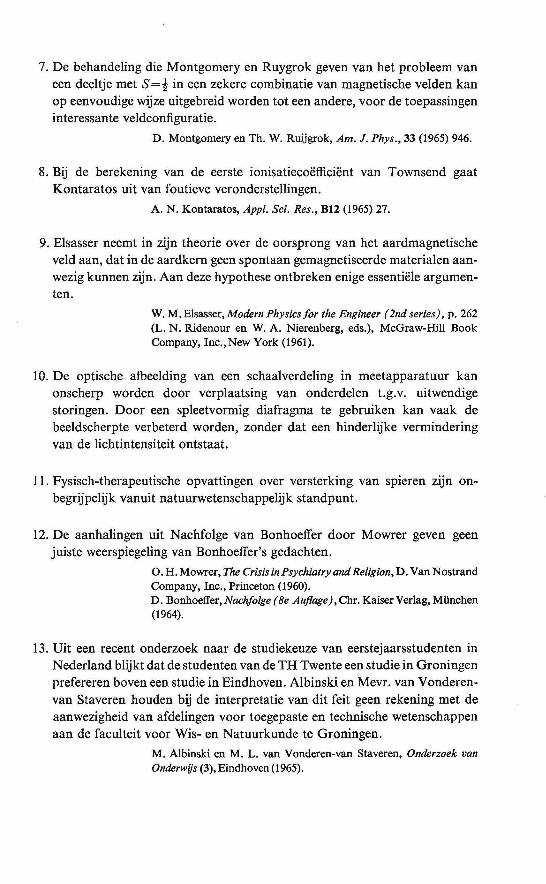
7. De behandeling die Montgomery en Ruygrok geven van het probleem van een deeltje met S=! in een zekere combinatie van magnetische velden kan op eenvoudige wijze uitgebreid worden tot een andere, voor de toepassingen interessante veldconfiguratie.
D. Montgomery en Th. W. Ruijgrok, Am. J. Phys., 33 (1965) 946.
8. Bij de berekening van de eerste ionisatiecoë:fficiënt van Townsend gaat Kontaratos uit van foutieve veronderstellingen.
A. N. Kontaratos, Appl. Sci. Res., B12 (1965) 27.
9. Elsasser neemt in zijn theorie over de oorsprong van het aardmagnetische veld aan, dat in de aardkern geen spontaan gemagnetiseerde materialen aanwezig kunnen zijn. Aan deze hypothese ontbreken enige essentiële argumenten.
W. M.Elsasser, Modern Physicsfor the Engineer (2nd series), p. 262 (L. N. Ridenour en W. A. Nierenberg, eds.), McGraw-Hill Book Company, Ine., New York (1961).
10. De optische afbeelding van een schaalverdeling in meetapparatuur kan onscherp worden door verplaatsing van onderdelen t.g.v. uitwendige storingen. Door een spleetvormig diafragma te gebruiken kan vaak de beeldscherpte verbeterd worden, zonder dat een hinderlijke vermindering van de lichtintensiteit ontstaat.
11. Fysisch-therapeutische opvattingen over versterking van spieren zijn onbegrijpelijk vanuit natuurwetenschappelijk standpunt.
12. De aanhalingen uit Nachfolge van Bonhoeffer door Mowrer geven geen juiste weerspiegeling van Bonhoeffer's gedachten.
0. H. Mowrer, The Crisis in Psychiatry and Re lig ion, D. Van N ostrand Company, Ine., Princeton (1960). D. Bonhoeffer, Nachfo/ge (Be Auflage), Chr. Kaiser Verlag, München (1964).
13. Uit een recent onderzoek naar de studiekeuze van eerstejaarsstudenten in Nederland blijkt dat de studenten van de TH Twente een studie in Groningen prefereren boven een studie in Eindhoven. Albinski en Mevr. van Vonderenvan Staveren houden bij de interpretatie van dit feit geen rekening met de aanwezigheid van afdelingen voor toegepaste en technische wetenschappen aan de faculteit voor Wis- en Natuurkunde te Groningen.
M. Albinski en M. L. van Vonderen-van Staveren, Onderzoek van Onderwijs (3), Eindhoven (1965).