examensarbete solving the generalized assignment problem by
TRANSCRIPT
Examensarbete
Solving the Generalized Assignment Problem by column
enumeration based on Lagrangian reduced costs
Peter Brommesson
LiTH - MAT - EX - - 2005 / 12 - - SE

Solving the Generalized Assignment Problem by column
enumeration based on Lagrangian reduced costs
Division of Optimization, Department of Mathematics , Linkoping University
Peter Brommesson
LiTH - MAT - EX - - 2005 / 12 - - SE
Examensarbete: 20 p
Level: D
Supervisors: Torbjorn Larsson,Division of Optimization, Department of Mathematics , Linkoping UniversityMaud Gothe-Lundgren,Division of Optimization, Department of Mathematics , Linkoping University
Examiner: Maud Gothe-Lundgren,Division of Optimization, Department of Mathematics , Linkoping University
Linkoping: January 2006

Matematiska Institutionen581 83 LINKOPINGSWEDEN
January 2006
x x
http://urn.kb.se/resolve?urn=urn:nbn:se:liu:diva-5583
LiTH - MAT - EX - - 2005 / 12 - - SE
Solving the Generalized Assignment Problem by column enumeration based on La-grangian reduced costs
Peter Brommesson
In this thesis a method for solving the Generalized Assignment Problem (GAP)is described. It is based on a reformulation of the original problem into a SetPartitioning Problem (SPP), in which the columns represent partial solutions tothe original problem. For solving this problem, column generation, with systematicovergeneration of columns, is used. Conditions that guarantee that an optimalsolution to a restricted SPP is optimal also in the original problem are given. Inorder to satisfy these conditions, not only columns with the most negative Lagrangianreduced costs need to be generated, but also others; this observation leads to the useof overgeneration of columns.
The Generalized Assignment Problem has shown to be NP-hard and therefore efficientalgorithms are needed, especially for large problems. The application of the proposedmethod decomposes GAP into several knapsack problems via Lagrangian relaxation,and enumerates solutions to each of these problems. The solutions obtained from theknapsack problems form a Set Partitioning Problem, which consists of combining onesolution from each knapsack problem to obtain a solution to the original problem.The algorithm has been tested on problems with 10 agents and 60 jobs. This leadsto 10 knapsack problems, each with 60 variables.
Generalized Assignment Problem, Knapsack Problems, Lagrangian Relaxation, Over-generation, Enumeration, Set Partitioning Problem.
Nyckelord
Keyword
Sammanfattning
Abstract
Forfattare
Author
Titel
Title
URL for elektronisk version
Serietitel och serienummer
Title of series, numbering
ISSN0348-2960
ISRN
ISBNSprak
Language
Svenska/Swedish
Engelska/English
Rapporttyp
Report category
Licentiatavhandling
Examensarbete
C-uppsats
D-uppsats
Ovrig rapport
Avdelning, Institution
Division, Department
Datum
Date

vi
Abstract
In this thesis a method for solving the Generalized Assignment Problem (GAP)is described. It is based on a reformulation of the original problem into a SetPartitioning Problem (SPP), in which the columns represent partial solutionsto the original problem. For solving this problem, column generation, with sys-tematic overgeneration of columns, is used. Conditions that guarantee that anoptimal solution to a restricted SPP is optimal also in the original problem aregiven. In order to satisfy these conditions, not only columns with the mostnegative Lagrangian reduced costs need to be generated, but also others; thisobservation leads to the use of overgeneration of columns.
The Generalized Assignment Problem has shown to be NP-hard and thereforeefficient algorithms are needed, especially for large problems. The applicationof the proposed method decomposes GAP into several knapsack problems viaLagrangian relaxation, and enumerates solutions to each of these problems. Thesolutions obtained from the knapsack problems form a Set Partitioning Problem,which consists of combining one solution from each knapsack problem to obtaina solution to the original problem. The algorithm has been tested on problemswith 10 agents and 60 jobs. This leads to 10 knapsack problems, each with 60variables.
Keywords: Generalized Assignment Problem, Knapsack Problems, LagrangianRelaxation, Overgeneration, Enumeration, Set Partitioning Problem.
Brommesson, 2006. vii

viii

Acknowledgments
I would like to thank my supervisors Maud Gothe-Lundgren and Torbjorn Lars-son for their guidance and help during this project.
I would also like to thank my opponent Anna Mahl for reading the reportcarefully and giving valuable criticism.
Finally, I would like to thank Mattias Eriksson for discussions regarding im-plementational issues.
Brommesson, 2006. ix

x
Contents
1 Introduction 1
1.1 The Generalized Assignment Problem . . . . . . . . . . . . . . . 11.2 Purpose . . . . . . . . . . . . . . . . . . . . . . . . . . . . . . . . 21.3 Outline of the thesis . . . . . . . . . . . . . . . . . . . . . . . . . 2
2 Background 3
2.1 Theoretical background . . . . . . . . . . . . . . . . . . . . . . . 32.2 A numerical example . . . . . . . . . . . . . . . . . . . . . . . . . 7
3 Method 9
3.1 Introduction to the method . . . . . . . . . . . . . . . . . . . . . 93.2 Finding near-optimal Lagrangian multipliers . . . . . . . . . . . 93.3 Finding feasible solutions and upper bounds to GAP . . . . . . . 103.4 Enumeration of knapsack solutions . . . . . . . . . . . . . . . . . 113.5 The Set Partitioning Problem . . . . . . . . . . . . . . . . . . . . 113.6 Parameter values . . . . . . . . . . . . . . . . . . . . . . . . . . . 12
3.6.1 The step length and number of iterations . . . . . . . . . 123.6.2 Feasible solutions and UBD . . . . . . . . . . . . . . . . . 123.6.3 The enumeration . . . . . . . . . . . . . . . . . . . . . . . 123.6.4 ρi in the numerical example . . . . . . . . . . . . . . . . 13
4 Tests, results and conclusions 15
4.1 The different tests . . . . . . . . . . . . . . . . . . . . . . . . . . 154.2 Variations in the quality of the near-optimal Lagrangian multipliers 154.3 Variation of κ . . . . . . . . . . . . . . . . . . . . . . . . . . . . 194.4 Variations of ρi, when equal for all i . . . . . . . . . . . . . . . . 224.5 Conclusions and future work . . . . . . . . . . . . . . . . . . . . 25
Brommesson, 2006. xi

xii Contents
Chapter 1
Introduction
1.1 The Generalized Assignment Problem
The Generalized Assignment Problem (GAP) is the problem of minimizing thecost of assigning n different items to m agents, such that each item is assignedto precisely one agent, subject to a capacity constraint for each agent. Thisproblem can be formulated as
[GAP ] min
m∑
i=1
n∑
j=1
cijxij
s.t.
n∑
j=1
aijxij ≤ bi, i = 1, . . . , m
m∑
i=1
xij = 1, j = 1, . . . , n
xij ∈ {0, 1}, i = 1, . . . , m,
j = 1, . . . , n.
Here, cij is the cost of assigning item j to agent i, aij is the claim on the ca-pacity of agent i by item j, and bi is the capacity of agent i.
GAP and its substructure appears in many problems, such as vehicle routingand facility location. GAP is known to be NP-hard (e.g. [4]) and therefore effi-cient algorithms is needed for its solution, especially for large problems. Manyexisting algorithms are based on using Lagrangian relaxation to decompose theproblem into m knapsack problems (e.g. [1],[9]).
Savelsbergh ([1]) uses a branch-and-price algorithm to solve GAP. This algo-rithm starts by solving the continuous relaxation of a Set Partitioning Problemreformulation of GAP by a column generation scheme. This is made in the rootnode of a branch-and-bound tree. Further, branching is performed to obtainan optimal integer solution to the Set Partitioning Problem. In this branching
Brommesson, 2006. 1
2 Chapter 1. Introduction
scheme, additional columns may be generated at any node in the branch-and-bound tree. The algorithm presented by Savelsbergh ([1]) guarantees the findingof an optimal solution, if feasible solutions exist.
Another algorithm that guarantees an optimal solution, is the one presentedby Nauss ([8]). This algorithm uses a special-purpose branch-and-bound algo-rithm to solve GAP. It is based on trying to prove that a valid lower bound isgreater or equal to a valid upper bound (if this can be shown, the upper boundis the optimal objective value). It uses minimal cover cuts, Lagrangian Relax-ation, penalties, feasibility based tests, and logical feasibility tests in order toincrease the lower bound, and feasible solution generators to decrease the upperbound.
Cattrysse et al. ([9]), present a heuristic Set Partitioning approach. They use acolumn generation procedure to generate knapsack solutions, and use these in aMaster Problem which has the form of a Set Partitioning Problem. This proce-dure, opposed to those presented in [1] and [8], does not guarantee an optimalsolution to GAP to be found.
1.2 Purpose
The main purpose of this thesis is to study a new method to solve the General-ized Assignment Problem, based on overgenerating columns to a Set Partition-ing Problem reformulation. The idea of this method is taken from a remark byLarsson and Patriksson ([11]). They propose an overgeneration of columns inthe root node in the branch-and-price algorithm presented by Savelsbergh ([1]),this in order to reduce, or completely remove, the need for further generation ofcolumns in the branch-and-bound tree. The proposal is based on the optimalityconditions that is presented by Larsson and Patriksson ([11]).
The algorithm presented in this thesis enumerates columns to the Set Parti-tioning Problem by solving knapsack problems (cf. [1] and [9]), and combinesat most one (typically exactly one) solution to every knapsack into a feasiblesolution to the Generalized Assignment Problem. We will study how the way ofenumerating knapsack solutions will affect the quality of the solution to Gener-alized Assignment Problem, obtained by solving a Set Partitioning Problem.
1.3 Outline of the thesis
Chapter 2 presents a theoretical background regarding the formulation of theGeneralized Assignment Problem as a Set Partitioning Problem and the gener-ation of knapsack solutions (i.e. columns). In Chapter 2, a numerical exampleof the theoretical discussion is also given. Chapter 3 gives a more detailed de-scription of the method and the different parameters that can be used to modifyit. Numerical tests, which are based on different values of the parameters, andresults are presented in Chapter 4. Chapter 4 also contains concluding remarksand suggestions for future research.
Chapter 2
Background
2.1 Theoretical background
The basic idea in this thesis is to reformulate the Generalized Assignment Prob-lem as a Set Partitioning Problem (SPP) and to enumerate columns to the latterproblem with respect to Lagrangian reduced cost. To find these columns, wedecompose the Generalized Assignment Problem via Lagrangian relaxation ofthe constraints that assert that every item is assigned to exactly one agent,and obtain m knapsack problems. Each knapsack problem corresponds to anagent in the original problem. By enumerating knapsack solutions (columns)it is possible to construct a Set Partitioning Problem, where each column rep-resents a knapsack solution. The Set Partitioning Problem can, in general, bedescribed as follows: Given a collection of subsets of a certain ground set andcosts associated with the subsets, the Set Partitioning Problem is the problemof finding a minimal cost partitioning of the ground set.
In this thesis, not only knapsack solutions with favorable sign of the reduced costare enumerated, but also knapsack solutions with “wrong” sign of the reducedcost. The reason for this is to obtain optimality in the integer Set PartitioningProblem. The theory presented by Larsson and Patriksson ([11]) motivates thisenumeration. They present global optimality and near-optimality conditions forthe Lagrangian formulation of an optimization problem. These conditions areconsistent for any size of the duality gap and provide, in our context, a possi-bility to assert optimality if specific knapsack solutions have been enumerated.The optimality condition are sufficient but not necessary, it is therefore reason-able to think that it is possible to find optimal solutions without fulfilling theseoptimality conditions.
Consider the Generalized Assignment Problem (GAP) with n items and m
Brommesson, 2006. 3
4 Chapter 2. Background
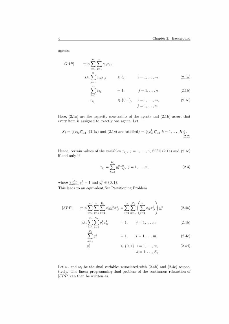
agents:
[GAP ] minm∑
i=1
n∑
j=1
cijxij
s.t.n∑
j=1
aijxij ≤ bi, i = 1, . . . , m (2.1a)
m∑
i=1
xij = 1, j = 1, . . . , n (2.1b)
xij ∈ {0, 1}, i = 1, . . . , m, (2.1c)
j = 1, . . . , n.
Here, (2.1a) are the capacity constraints of the agents and (2.1b) assert thatevery item is assigned to exactly one agent. Let
Xi = {(xij)nj=1| (2.1a) and (2.1c) are satisfied} = {(xk
ij)nj=1|k = 1, . . . , Ki}.
(2.2)
Hence, certain values of the variables xij , j = 1, . . . , n, fulfill (2.1a) and (2.1c)if and only if
xij =
Ki∑
k=1
yki xk
ij , j = 1, . . . , n, (2.3)
where∑Ki
k=1 yki = 1 and yk
i ∈ {0, 1}.
This leads to an equivalent Set Partitioning Problem
[SPP ] min
m∑
i=1
n∑
j=1
Ki∑
k=1
cijyki xk
ij =
m∑
i=1
Ki∑
k=1
n∑
j=1
cijxkij
yki (2.4a)
s.t.
m∑
i=1
Ki∑
k=1
yki xk
ij = 1, j = 1, . . . , n (2.4b)
Ki∑
k=1
yki = 1, i = 1, . . . , m (2.4c)
yki ∈ {0, 1} i = 1, . . . , m, (2.4d)
k = 1, . . . , Ki.
Let uj and wi be the dual variables associated with (2.4b) and (2.4c) respec-tively. The linear programming dual problem of the continuous relaxation of[SPP ] can then be written as
2.1. Theoretical background 5
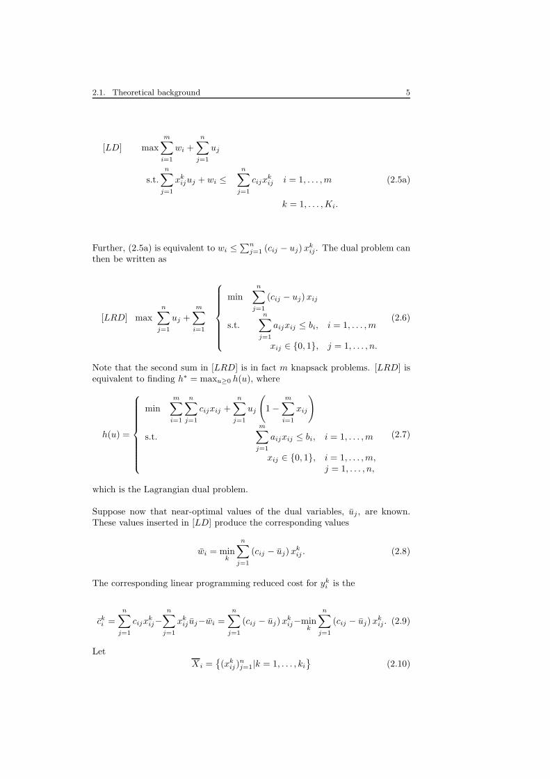
[LD] max
m∑
i=1
wi +
n∑
j=1
uj
s.t.
n∑
j=1
xkijuj + wi ≤
n∑
j=1
cijxkij i = 1, . . . , m (2.5a)
k = 1, . . . , Ki.
Further, (2.5a) is equivalent to wi ≤∑n
j=1 (cij − uj) xkij . The dual problem can
then be written as
[LRD] maxn∑
j=1
uj +m∑
i=1
minn∑
j=1
(cij − uj)xij
s.t.
n∑
j=1
aijxij ≤ bi, i = 1, . . . , m
xij ∈ {0, 1}, j = 1, . . . , n.
(2.6)
Note that the second sum in [LRD] is in fact m knapsack problems. [LRD] isequivalent to finding h∗ = maxu≥0 h(u), where
h(u) =
minm∑
i=1
n∑
j=1
cijxij +n∑
j=1
uj
(
1 −m∑
i=1
xij
)
s.t.
m∑
j=1
aijxij ≤ bi, i = 1, . . . , m
xij ∈ {0, 1}, i = 1, . . . , m,j = 1, . . . , n,
(2.7)
which is the Lagrangian dual problem.
Suppose now that near-optimal values of the dual variables, uj , are known.These values inserted in [LD] produce the corresponding values
wi = mink
n∑
j=1
(cij − uj)xkij . (2.8)
The corresponding linear programming reduced cost for yki is the
cki =
n∑
j=1
cijxkij−
n∑
j=1
xkij uj−wi =
n∑
j=1
(cij − uj)xkij−min
k
n∑
j=1
(cij − uj) xkij . (2.9)
Let
X i ={
(xkij)
nj=1|k = 1, . . . , ki
}
(2.10)
6 Chapter 2. Background
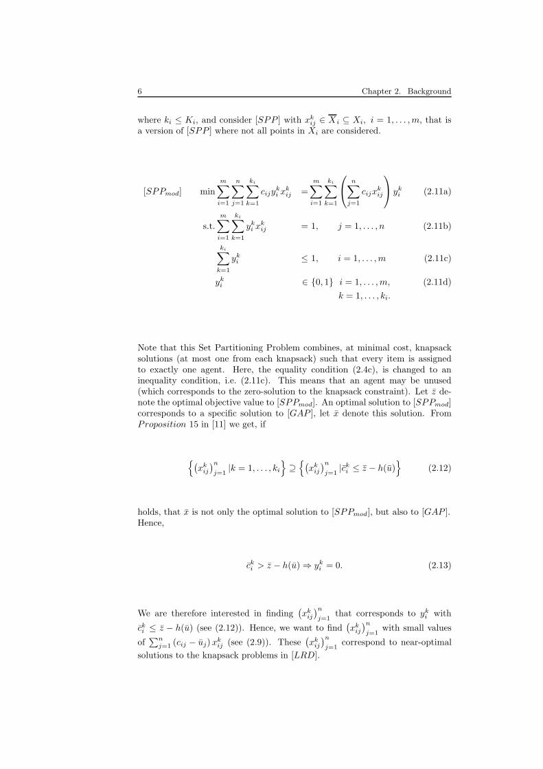
where ki ≤ Ki, and consider [SPP ] with xkij ∈ X i ⊆ Xi, i = 1, . . . , m, that is
a version of [SPP ] where not all points in Xi are considered.
[SPPmod] minm∑
i=1
n∑
j=1
ki∑
k=1
cijyki xk
ij =m∑
i=1
ki∑
k=1
n∑
j=1
cijxkij
yki (2.11a)
s.t.
m∑
i=1
ki∑
k=1
yki xk
ij = 1, j = 1, . . . , n (2.11b)
ki∑
k=1
yki ≤ 1, i = 1, . . . , m (2.11c)
yki ∈ {0, 1} i = 1, . . . , m, (2.11d)
k = 1, . . . , ki.
Note that this Set Partitioning Problem combines, at minimal cost, knapsacksolutions (at most one from each knapsack) such that every item is assignedto exactly one agent. Here, the equality condition (2.4c), is changed to aninequality condition, i.e. (2.11c). This means that an agent may be unused(which corresponds to the zero-solution to the knapsack constraint). Let z de-note the optimal objective value to [SPPmod]. An optimal solution to [SPPmod]corresponds to a specific solution to [GAP ], let x denote this solution. FromProposition 15 in [11] we get, if
{
(
xkij
)n
j=1|k = 1, . . . , ki
}
⊇{
(
xkij
)n
j=1|ck
i ≤ z − h(u)}
(2.12)
holds, that x is not only the optimal solution to [SPPmod], but also to [GAP ].Hence,
cki > z − h(u) ⇒ yk
i = 0. (2.13)
We are therefore interested in finding(
xkij
)n
j=1that corresponds to yk
i with
cki ≤ z − h(u) (see (2.12)). Hence, we want to find
(
xkij
)n
j=1with small values
of∑n
j=1 (cij − uj)xkij (see (2.9)). These
(
xkij
)n
j=1correspond to near-optimal
solutions to the knapsack problems in [LRD].
2.2. A numerical example 7
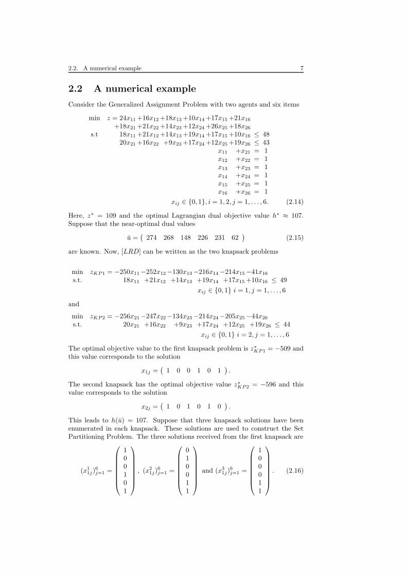
2.2 A numerical example
Consider the Generalized Assignment Problem with two agents and six items
min z = 24x11 +16x12 +18x13 +10x14 +17x15 +21x16
+18x21 +21x22 +14x23 +12x24 +26x25 +18x26
s.t 18x11 +21x12 +14x13 +19x14 +17x15 +10x16 ≤ 4820x21 +16x22 +9x23 +17x24 +12x25 +19x26 ≤ 43
x11 +x21 = 1x12 +x22 = 1x13 +x23 = 1x14 +x24 = 1x15 +x25 = 1x16 +x26 = 1
xij ∈ {0, 1}, i = 1, 2, j = 1, . . . , 6. (2.14)
Here, z∗ = 109 and the optimal Lagrangian dual objective value h∗ ≈ 107.Suppose that the near-optimal dual values
u =(
274 268 148 226 231 62)
(2.15)
are known. Now, [LRD] can be written as the two knapsack problems
min zKP1 = −250x11 −252x12 −130x13 −216x14 −214x15 −41x16
s.t. 18x11 +21x12 +14x13 +19x14 +17x15 +10x16 ≤ 49
xij ∈ {0, 1} i = 1, j = 1, . . . , 6
and
min zKP2 = −256x21 −247x22 −134x23 −214x24 −205x25 −44x26
s.t. 20x21 +16x22 +9x23 +17x24 +12x25 +19x26 ≤ 44
xij ∈ {0, 1} i = 2, j = 1, . . . , 6
The optimal objective value to the first knapsack problem is z∗KP1 = −509 andthis value corresponds to the solution
x1j =(
1 0 0 1 0 1)
.
The second knapsack has the optimal objective value z∗KP2 = −596 and thisvalue corresponds to the solution
x2j =(
1 0 1 0 1 0)
.
This leads to h(u) = 107. Suppose that three knapsack solutions have beenenumerated in each knapsack. These solutions are used to construct the SetPartitioning Problem. The three solutions received from the first knapsack are
(x11j)
6j=1 =
100101
, (x21j)
6j=1 =
010011
and (x31j)
6j=1 =
100011
. (2.16)
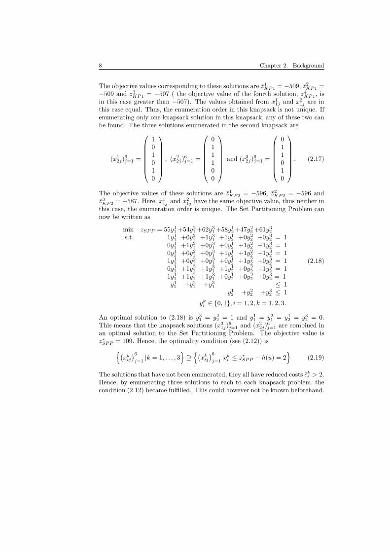
8 Chapter 2. Background
The objective values corresponding to these solutions are z1KP1 = −509, z2
KP1 =−509 and z3
KP1 = −507 ( the objective value of the fourth solution, z4KP1, is
in this case greater than −507). The values obtained from x11j and x2
1j are inthis case equal. Thus, the enumeration order in this knapsack is not unique. Ifenumerating only one knapsack solution in this knapsack, any of these two canbe found. The three solutions enumerated in the second knapsack are
(x12j)
6j=1 =
101010
, (x22j)
6j=1 =
011100
and (x32j)
6j=1 =
011010
. (2.17)
The objective values of these solutions are z1KP2 = −596, z2
KP2 = −596 andz3
KP2 = −587. Here, x11j and x2
1j have the same objective value, thus neither inthis case, the enumeration order is unique. The Set Partitioning Problem cannow be written as
min zSPP = 55y11 +54y2
1 +62y31 +58y1
2 +47y22 +61y3
2
s.t 1y11 +0y2
1 +1y31 +1y1
2 +0y22 +0y3
2 = 10y1
1 +1y21 +0y3
1 +0y12 +1y2
2 +1y32 = 1
0y11 +0y2
1 +0y31 +1y1
2 +1y22 +1y3
2 = 11y1
1 +0y21 +0y3
1 +0y12 +1y2
2 +0y32 = 1
0y11 +1y2
1 +1y31 +1y1
2 +0y22 +1y3
2 = 11y1
1 +1y21 +1y3
1 +0y12 +0y2
2 +0y32 = 1
y11 +y2
1 +y31 ≤ 1
y12 +y2
2 +y32 ≤ 1
(2.18)
yki ∈ {0, 1}, i = 1, 2, k = 1, 2, 3.
An optimal solution to (2.18) is y31 = y2
2 = 1 and y11 = y2
1 = y12 = y3
2 = 0.This means that the knapsack solutions (x3
1j)6j=1 and (x2
2j)6j=1 are combined in
an optimal solution to the Set Partitioning Problem. The objective value isz∗SPP = 109. Hence, the optimality condition (see (2.12)) is
{
(
xkij
)6
j=1|k = 1, . . . , 3
}
⊇{
(
xkij
)6
j=1|ck
i ≤ z∗SPP − h(u) = 2}
(2.19)
The solutions that have not been enumerated, they all have reduced costs cki > 2.
Hence, by enumerating three solutions to each to each knapsack problem, thecondition (2.12) became fulfilled. This could however not be known beforehand.
Chapter 3
Method
3.1 Introduction to the method
This thesis presents a Set Partitioning approach to solve GAP, based on thegeneration of feasible solutions to knapsack problems. This approach is similarto those presented in [1] and [9]. The main difference is how knapsack solutionsare generated and, different from [9], the possibility to assert optimality (see(2.12)). Even though optimal values of the dual variables for the constraints(2.1b) are not known, it is possible (due to (2.12)) to assert optimality. Cat-trysse et al. ([9]) use a column generation procedure that repeatedly generatesknapsack solutions, while we enumerate knapsack solutions only once, whennear-optimal values of the dual variables are known. One of the similaritiesbetween [9] and our approach, is the procedure to obtain near-optimal valuesof the dual variables corresponding to (2.1b). Both methods use a subgradientscheme to obtain these values.
Our method consists of the following steps:
1. (a) Find a lower bound to GAP and near-optimal Lagrangian multipliersfor (2.1b) via a subgradient scheme.
(b) Find a feasible solution and an upper bound to GAP.
2. Enumerate solutions to the knapsack problems in [LRD], given knownnear-optimal Lagrangian multipliers.
3. Solve the resulting [SPPmod] with the obtained knapsack solutions.
3.2 Finding near-optimal Lagrangian multipli-
ers
A fast method for finding near-optimal Lagrangian multipliers and a lowerbound to GAP is the subgradient optimization method. The goal is to findnear-optimal (or optimal) u in [LRD], which are then used to determine howto enumerate knapsack solutions. To find this near-optimal u a subgradientscheme is implemented, where γj = 1 −
∑m
i=1 xij is the subgradient used (i.e.
Brommesson, 2006. 9
10 Chapter 3. Method
the subgradient that corresponds to (2.1b)). In this procedure we initially setthe Lagrangian multipliers u = 0, the lower bound LBD = 0, and the upperbound UBD = M , were M is a very large number. In every iteration q, for givenuq, [LRD], i.e. the m knapsack problems are solved. This solution provides anLBD to [GAP ], defined as LBD = max(LBD, h(uq)). In every iteration, theLagrangian multipliers are updated according to uq+1 = uq + tqγq, where tq isthe step length in the subgradient scheme. Here, tq is defined as
tq =λq (UBD − h(uq))
‖γq‖2(3.1)
where λq is a parameter to be chosen (typically λ ∈ (0, 2)). This is a modificationof the Polyak step length where UBD = h∗, the optimal dual objective value,and 0 < ǫ1 ≤ λk ≤ 2−ǫ2 < 2. The values of λq and UBD will change throughoutthe iterations, and change the step length. The termination criterion for thesubgradient scheme is simply a maximal number of iterations. The choice ofthis number of iterations, the values of λq and the UBD will be discussed later.
3.3 Finding feasible solutions and upper bounds
to GAP
The subgradient scheme does not only provide a near-optimal dual solution u,but also knapsack solutions. Based on the knapsack solutions provided in thesubgradient scheme, a heuristic method to find feasible solutions to [GAP ] isimplemented. This heuristic is based on a strategy presented by Fisher ([3]).Since (2.1b) is dualized, these constraints may be violated. Thus, the itemscan be partitioned into three sets, depending on how many times each item isassigned to the agents. Letting x∗ denote an optimal solution to [LRD], thesesets can be defined as
S1 =
{
j ∈ J |
m∑
i=1
x∗ij = 0
}
S2 =
{
j ∈ J |m∑
i=1
x∗ij = 1
}
S3 =
{
j ∈ J |
m∑
i=1
x∗ij > 1
}
.
(3.2)
The constraints of [GAP ] that are violated correspond to j ∈ S1 ∪ S3. To finda feasible solution to [GAP ], a modification of x∗ corresponding to j ∈ S1 ∪ S3
is needed. This is easy for an item j ∈ S3. By removing the item j from allbut one knapsack, the constraint corresponding to this item is fulfilled. Thereare several ways to determine in which knapsack item j should be left (andthis will be discussed later). The critical set is S1. To fulfill the constraintcorresponding to item j ∈ S1, this item is assigned to the agent that minimizesthe cost without exceeding (2.1a). Although this procedure does not guarantee
3.4. Enumeration of knapsack solutions 11
a feasible solution to be found, tests show that the chances of finding one israther good. The feasible solution provides a UBD, which is used to calculatethe step length t.
3.4 Enumeration of knapsack solutions
The enumeration is reduced cost based, i.e. it ranks the knapsack solutionsaccording to reduced costs. The enumeration used in this thesis is based ona procedure presented by Revenius ([6]), which is a modification of a branch-and-bound algorithm for solving the binary knapsack problem ([2]). Below, thisprocedure is presented for a maximization problem. The enumeration startswith all xi = 0 and the variables ordered according to non-increasing efficienciesei = ci/ai. The purpose of starting with xi = 0, i = 1 . . . n, is to examine everybranch in the branch-and-bound tree. Let
C =
n∑
i=1
cixi and A =
n∑
i=1
aixi. (3.3)
Further, let t be an integer and let xi be fixed for i ∈ [1, t]. In the first branchingstep, n branches are created, each with one variable xi = 1. In every branch,let t = i. In the following steps, if A ≤ b, an item i > t is added to the knapsackand then t is set equal to i. This means that the t first items are fixed and thatthe branching is made over the n − t remaining items. If t = n (i.e. if t is thelast element) the branch is terminated, since all items have been used.
The number of solutions to be enumerated can be decided by either a maximumnumber of solutions or a parameter ρ ∈ [0, 1], which controls that solutions thathave objective values greater than ρz∗ are saved. The parameter ρ combinedwith the Dantzig upper bound, which is obtained by a continuous relaxation ofthe knapsack problem ([12]), provides a new upper bound which can be usedfor terminating the branching. Let z′ denote the best objective value found sofar. Then, a branch is terminated if A > b, or if A ≤ b and
C +(b − A)ct
at
< ρz′. (3.4)
That is, a branch is terminated if the capacity constraint is violated or if theupper bound is less than ρ ∗ 100 percent of the best solution found.
The best near-optimal solutions are saved in a complete binary min-heap. If anew near-optimal solution is found, and the heap is full, the newly found solu-tion is compared with the root-node, which is the solution in the heap with thelowest objective value. If the new solution is better than this solution, the newsolution is placed in the root-node and a percolate-down procedure is appliedto this node.
3.5 The Set Partitioning Problem
When near-optimal Lagrangian multipliers are known, these are used to enu-merate knapsack solutions. In the most favorable case, (2.12) holds when the
12 Chapter 3. Method
enumeration has been made. The enumeration of knapsack solutions strives tofulfill (2.12), and if this is successful, optimality in [GAP ] can be guaranteed.Since (2.12) is only a sufficient and not a necessary condition, this condition doesnot have to be fulfilled to obtain an optimal solution. Thus, hopefully less enu-merated knapsack solutions are needed, than (2.12) indicates. The enumeratedsolutions are used to construct the Set Partitioning Problem, [SPPmod]. Thenumber of enumerated solutions in each knapsack may vary, depending on theuser-defined maximum number of solutions, and/or the deviation between theoptimal solution and the enumerated ones. The knapsack solutions correspondto the points
(
xkij
)n
j=1in [SPPmod], i.e. there are ki solutions to every knapsack
constraint. One solution in every knapsack constraint should be chosen, subjectto that every item j is assigned to exactly one agent.
3.6 Parameter values
3.6.1 The step length and number of iterations
The step length (3.1) depends on the value of λq. There are several ways tochoose this parameter. It can be set to a fixed value throughout the subgradi-ent iterations but it can also be chosen to decrease in each iteration. This cansometimes be efficient. The reason for this strategy is to initially choose a largerstep, in order to quickly reach the neighborhood of the optimal solution. Thereason to choose a smaller step length in each iteration, is to ensure quick con-vergence to the optimal solution. In our experiments, λq = 0.999q. The Polyakstep length (presented in Section 3.2) ensures that the subgradient scheme willeventually provide us with an optimal solution (see [13]). By using λq = 0.999q
instead of 0 < ǫ1 ≤ λq ≤ 2 − ǫ2 < 2, and UBD instead of h∗, convergence toan optimum can not be asserted. This step length however works well in prac-tice. We choose to stop the subgradient scheme when the number of iterationsreaches a predefined number. In the tests, this number has been chosen between30 and 1000.
3.6.2 Feasible solutions and UBD
The upper bound, UBD, is the cost of the best available feasible solution to[GAP ]. The heuristic method for finding these solutions is as presented byFisher ([3]), but the criterion which determines in which knapsack an itemj ∈ S3 should be left, may be chosen in different ways. One way is to leave theitem in the knapsack that minimizes (cij − uj). Another possible choice is toconsider the ratio −(cij −uj)/aij . By doing so, the capacity that item j uses inknapsack i (corresponding to the capacity constraint in [LRD]), is considered.The first alternative is used in this thesis.
3.6.3 The enumeration
The number of solutions to be enumerated in each knapsack is in the tests(described in next the chapter) initially set fixed. As mentioned in Section 3.4,there is a second parameter, that controls the maximum allowed deviation fromthe optimal knapsack solution. Letting z∗i denote the value of the best, with
3.6. Parameter values 13
respect to Lagrangian reduced cost, enumerated knapsack solution for knapsacki, this parameter is defined as
ρi = 1 − κUBD − LBD
m|z∗i |, (3.5)
where κ is a parameter that may be chosen differently in each test. The purposeof this definition of ρi is to stop the enumeration in the knapsacks where it islikely that no further enumeration is needed. That is, when the objective value ofthe latest enumerated solution, in a specific knapsack i, is greater than ρi∗100%of the best solution found for this knapsack, the enumeration for this knapsackstops. Thus, ρi prevents enumeration of knapsack solutions that are not likelyto be a part of the optimal solution to [SPP ].
3.6.4 ρi in the numerical example
When enumerating knapsack solutions, the optimal objective value to (2.14) isof course not known. Suppose that a solution to (2.14) with objective value116 is known. This gives an upper bound, UBD = 116. Let further κ = 1.Application of these values leads to
ρ1 ≈ 0.9921 and ρ2 ≈ 0.9933. (3.6)
If these values of ρi are considered in (2.14), the number of knapsack solutionsto be enumerated are three and two, respectively. These knapsack solutionsprovide an optimal solution to (2.14). To assert optimality by means of (2.12),with z = 116 and h(u) = 107, the number of solutions enumerated would haveto be four and three, respectively. When (2.18) has been solved, optimalitycan be asserted. Its optimal objective value is z∗SPP = 109, and if this valueis used in (2.12) we can conclude that further enumeration does not lead to animprovement of the objective value in (2.14).

14 Chapter 3. Method
Chapter 4
Tests, results and
conclusions
4.1 The different tests
The tests performed in this thesis are all on maximization problems with 10agents and 60 items. The resource requirements aij are integers from the uni-form distribution U(5, 25), the cost coefficients cij are integers from U(15, 25)and the capacity of agent i is bi = 0.8
∑n
j=1 aij/10. These test problems arenamed gap12a - gap12e and are taken from [10]. In the tests performed, thekey-question was: Under what conditions, is a feasible solution and an optimalsolution obtained? Three variations were considered in the tests:
1. Variation in the quality of the near-optimal Lagrangian multipliers.
2. Variation of κ in (3.5).
3. Variation of ρi, when equal for every i.
4.2 Variations in the quality of the near-optimal
Lagrangian multipliers
If near-optimal Lagrangian multipliers are known, it is possible to assert opti-mality by means of 2.12. It seems likely that fewer solutions are needed to beenumerated the greater h(u) is, i.e. the closer h(u) is to the optimal value h(u∗).Note that although this seems highly probable, it need not always be the case.To study how the quality of the Lagrangian multipliers affect the the numberof solutions needed to find a feasible and an optimal solution, respectively, dif-ferent numbers of subgradient iterations have been used. The tests have beenperformed with 30, 40, 50, 100, 200, 500 and 1000 subgradient iterations, andthese different numbers of subgradient iterations result in different values ofh(u). There may exist other sets of multipliers that give the same value ofh(u) as the ones shown in the following figures. Thus, the enumeration is notunique for the values of h(u) obtained from the Lagrangian multipliers used here.
Brommesson, 2006. 15
16 Chapter 4. Tests, results and conclusions
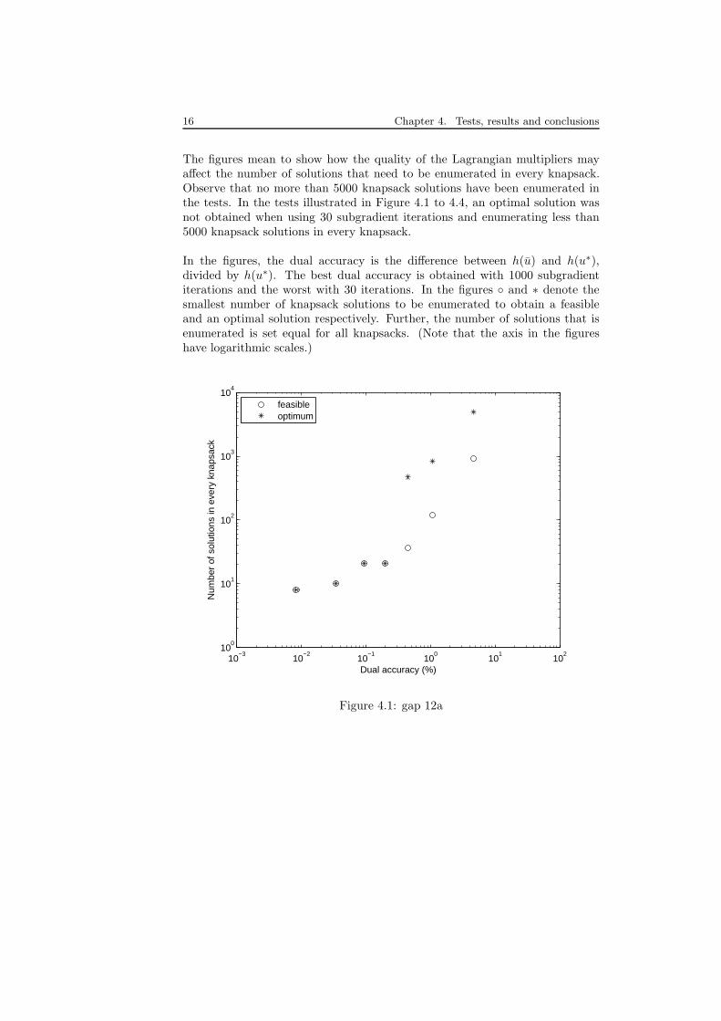
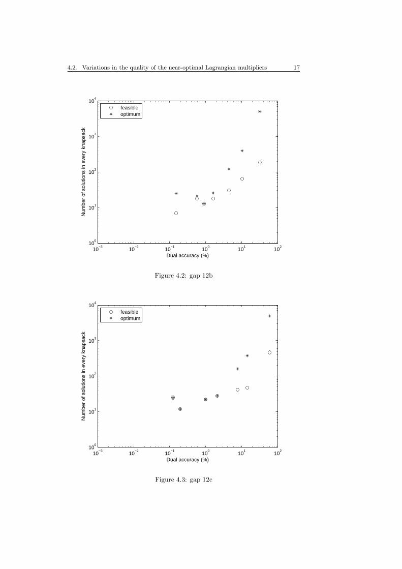
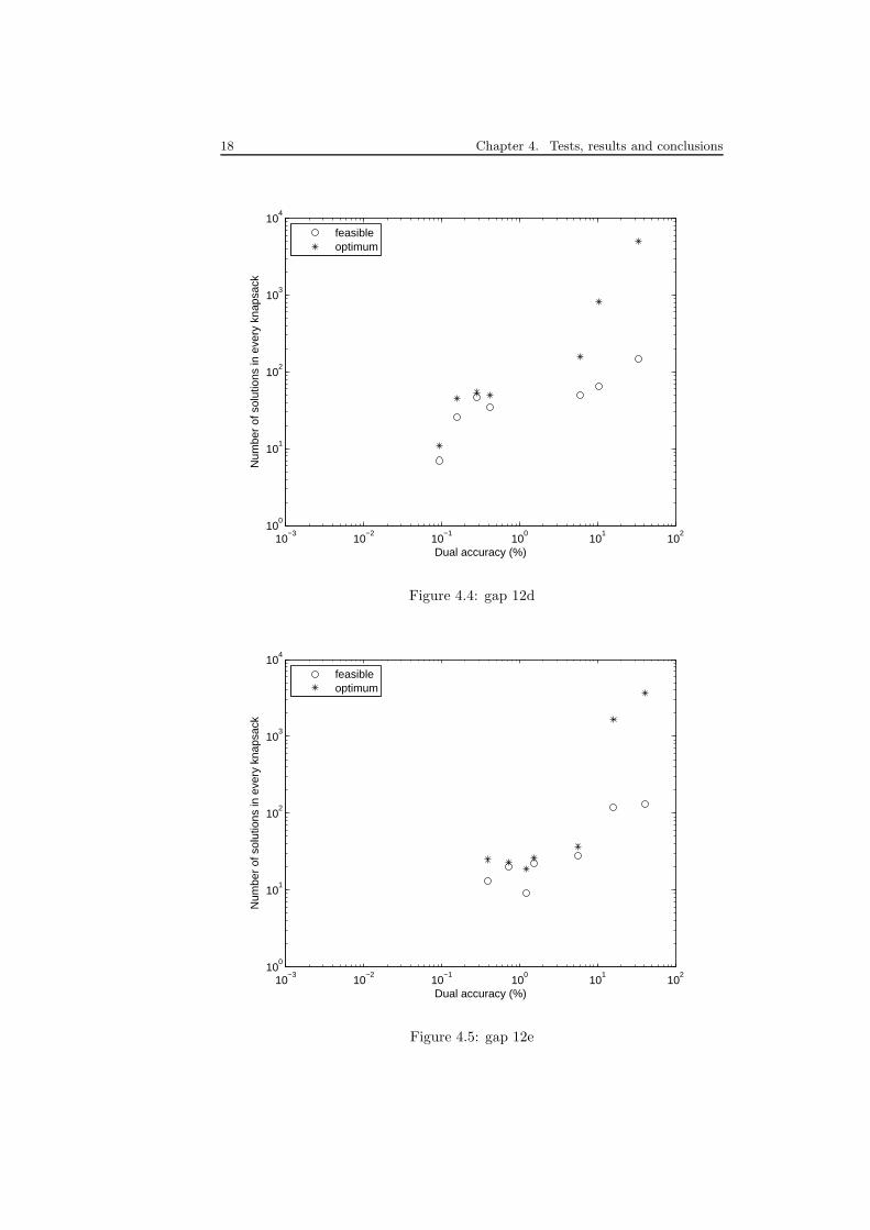
The figures mean to show how the quality of the Lagrangian multipliers mayaffect the number of solutions that need to be enumerated in every knapsack.Observe that no more than 5000 knapsack solutions have been enumerated inthe tests. In the tests illustrated in Figure 4.1 to 4.4, an optimal solution wasnot obtained when using 30 subgradient iterations and enumerating less than5000 knapsack solutions in every knapsack.
In the figures, the dual accuracy is the difference between h(u) and h(u∗),divided by h(u∗). The best dual accuracy is obtained with 1000 subgradientiterations and the worst with 30 iterations. In the figures ◦ and ∗ denote thesmallest number of knapsack solutions to be enumerated to obtain a feasibleand an optimal solution respectively. Further, the number of solutions that isenumerated is set equal for all knapsacks. (Note that the axis in the figureshave logarithmic scales.)
10−3
10−2
10−1
100
101
102
100
101
102
103
104
Dual accuracy (%)
Num
ber
of s
olut
ions
in e
very
kna
psac
k
feasibleoptimum
Figure 4.1: gap 12a
4.2. Variations in the quality of the near-optimal Lagrangian multipliers 17
10−3
10−2
10−1
100
101
102
100
101
102
103
104
Dual accuracy (%)
Num
ber
of s
olut
ions
in e
very
kna
psac
k
feasibleoptimum
Figure 4.2: gap 12b
10−3
10−2
10−1
100
101
102
100
101
102
103
104
Dual accuracy (%)
Num
ber
of s
olut
ions
in e
very
kna
psac
k
feasibleoptimum
Figure 4.3: gap 12c
18 Chapter 4. Tests, results and conclusions
10−3
10−2
10−1
100
101
102
100
101
102
103
104
Dual accuracy (%)
Num
ber
of s
olut
ions
in e
very
kna
psac
k
feasibleoptimum
Figure 4.4: gap 12d
10−3
10−2
10−1
100
101
102
100
101
102
103
104
Dual accuracy (%)
Num
ber
of s
olut
ions
in e
very
kna
psac
k
feasibleoptimum
Figure 4.5: gap 12e
4.3. Variation of κ 19
The figures above indicate that if the dual accuracy is relatively good, thenumbers of knapsack solutions needed to find a feasible respective an optimalsolution, are very close. On the other hand, as the difference between h(u∗)and h(u) increases, the difference between the number of knapsack solutionsneeded increases. The figures also indicate that for all reasonable small valuesof the difference h(u∗)−h(u), there is no remarkable difference in the number ofknapsack solutions needed to obtain neither optimality nor a feasible solution.The number of solutions needed may even increase if h(u∗) − h(u) decreases.
4.3 Variation of κ
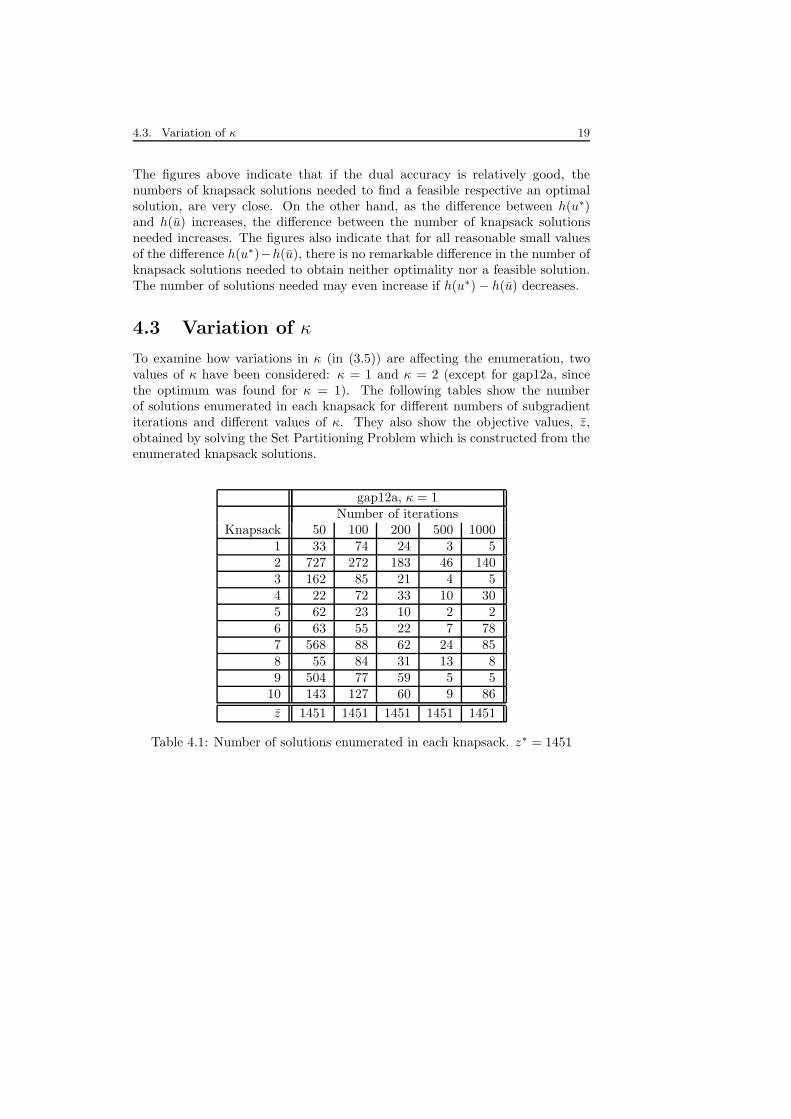
To examine how variations in κ (in (3.5)) are affecting the enumeration, twovalues of κ have been considered: κ = 1 and κ = 2 (except for gap12a, sincethe optimum was found for κ = 1). The following tables show the numberof solutions enumerated in each knapsack for different numbers of subgradientiterations and different values of κ. They also show the objective values, z,obtained by solving the Set Partitioning Problem which is constructed from theenumerated knapsack solutions.
gap12a, κ = 1Number of iterations
Knapsack 50 100 200 500 10001 33 74 24 3 52 727 272 183 46 1403 162 85 21 4 54 22 72 33 10 305 62 23 10 2 26 63 55 22 7 787 568 88 62 24 858 55 84 31 13 89 504 77 59 5 5
10 143 127 60 9 86
z 1451 1451 1451 1451 1451
Table 4.1: Number of solutions enumerated in each knapsack. z∗ = 1451
20 Chapter 4. Tests, results and conclusions
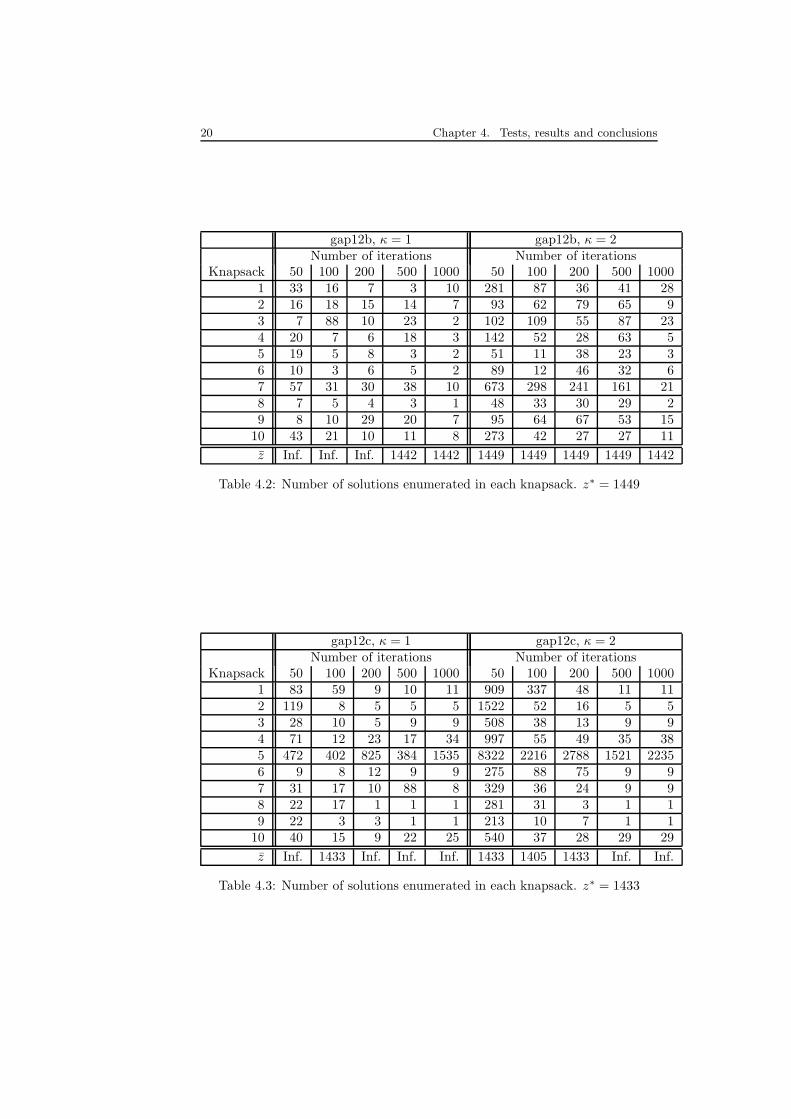
gap12b, κ = 1 gap12b, κ = 2Number of iterations Number of iterations
Knapsack 50 100 200 500 1000 50 100 200 500 10001 33 16 7 3 10 281 87 36 41 282 16 18 15 14 7 93 62 79 65 93 7 88 10 23 2 102 109 55 87 234 20 7 6 18 3 142 52 28 63 55 19 5 8 3 2 51 11 38 23 36 10 3 6 5 2 89 12 46 32 67 57 31 30 38 10 673 298 241 161 218 7 5 4 3 1 48 33 30 29 29 8 10 29 20 7 95 64 67 53 15
10 43 21 10 11 8 273 42 27 27 11
z Inf. Inf. Inf. 1442 1442 1449 1449 1449 1449 1442
Table 4.2: Number of solutions enumerated in each knapsack. z∗ = 1449
gap12c, κ = 1 gap12c, κ = 2Number of iterations Number of iterations
Knapsack 50 100 200 500 1000 50 100 200 500 10001 83 59 9 10 11 909 337 48 11 112 119 8 5 5 5 1522 52 16 5 53 28 10 5 9 9 508 38 13 9 94 71 12 23 17 34 997 55 49 35 385 472 402 825 384 1535 8322 2216 2788 1521 22356 9 8 12 9 9 275 88 75 9 97 31 17 10 88 8 329 36 24 9 98 22 17 1 1 1 281 31 3 1 19 22 3 3 1 1 213 10 7 1 1
10 40 15 9 22 25 540 37 28 29 29
z Inf. 1433 Inf. Inf. Inf. 1433 1405 1433 Inf. Inf.
Table 4.3: Number of solutions enumerated in each knapsack. z∗ = 1433
4.3. Variation of κ 21
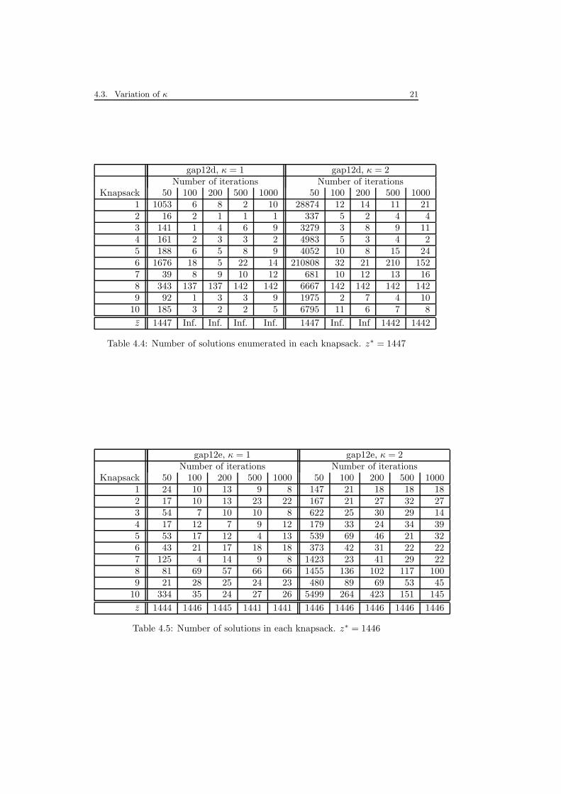
gap12d, κ = 1 gap12d, κ = 2Number of iterations Number of iterations
Knapsack 50 100 200 500 1000 50 100 200 500 10001 1053 6 8 2 10 28874 12 14 11 212 16 2 1 1 1 337 5 2 4 43 141 1 4 6 9 3279 3 8 9 114 161 2 3 3 2 4983 5 3 4 25 188 6 5 8 9 4052 10 8 15 246 1676 18 5 22 14 210808 32 21 210 1527 39 8 9 10 12 681 10 12 13 168 343 137 137 142 142 6667 142 142 142 1429 92 1 3 3 9 1975 2 7 4 10
10 185 3 2 2 5 6795 11 6 7 8
z 1447 Inf. Inf. Inf. Inf. 1447 Inf. Inf 1442 1442
Table 4.4: Number of solutions enumerated in each knapsack. z∗ = 1447
gap12e, κ = 1 gap12e, κ = 2Number of iterations Number of iterations
Knapsack 50 100 200 500 1000 50 100 200 500 10001 24 10 13 9 8 147 21 18 18 182 17 10 13 23 22 167 21 27 32 273 54 7 10 10 8 622 25 30 29 144 17 12 7 9 12 179 33 24 34 395 53 17 12 4 13 539 69 46 21 326 43 21 17 18 18 373 42 31 22 227 125 4 14 9 8 1423 23 41 29 228 81 69 57 66 66 1455 136 102 117 1009 21 28 25 24 23 480 89 69 53 45
10 334 35 24 27 26 5499 264 423 151 145
z 1444 1446 1445 1441 1441 1446 1446 1446 1446 1446
Table 4.5: Number of solutions in each knapsack. z∗ = 1446
22 Chapter 4. Tests, results and conclusions
The tables indicate that no general conclusions of neither the number of knap-sack solutions nor the objective value of the corresponding Set PartitioningProblem can be made. The expression (3.5) indicates however, that if there isa big difference between the upper bound and the lower bound, the value of ρi
tends to be small, which implies that more solutions need to be enumerated.But since the difference between the upper bound and the lower bound is large,it is likely that more knapsack solutions are needed to obtain a feasible or anoptimal solution. If a particular set of Lagrangian multipliers is considered, i.e.the difference between the upper bound and the lower bound is fix for everyknapsack. Then, the difference in the number of solutions in every knapsackis depending on the variation of z∗i (for each i), and the number of solutionsthat are close to the optimal solution in a certain knapsack. If there is a bigdifference between z∗i for different i, there will be a big difference in ρi as well.This will most likely lead to differences in the number of enumerated solutionsin the knapsacks.
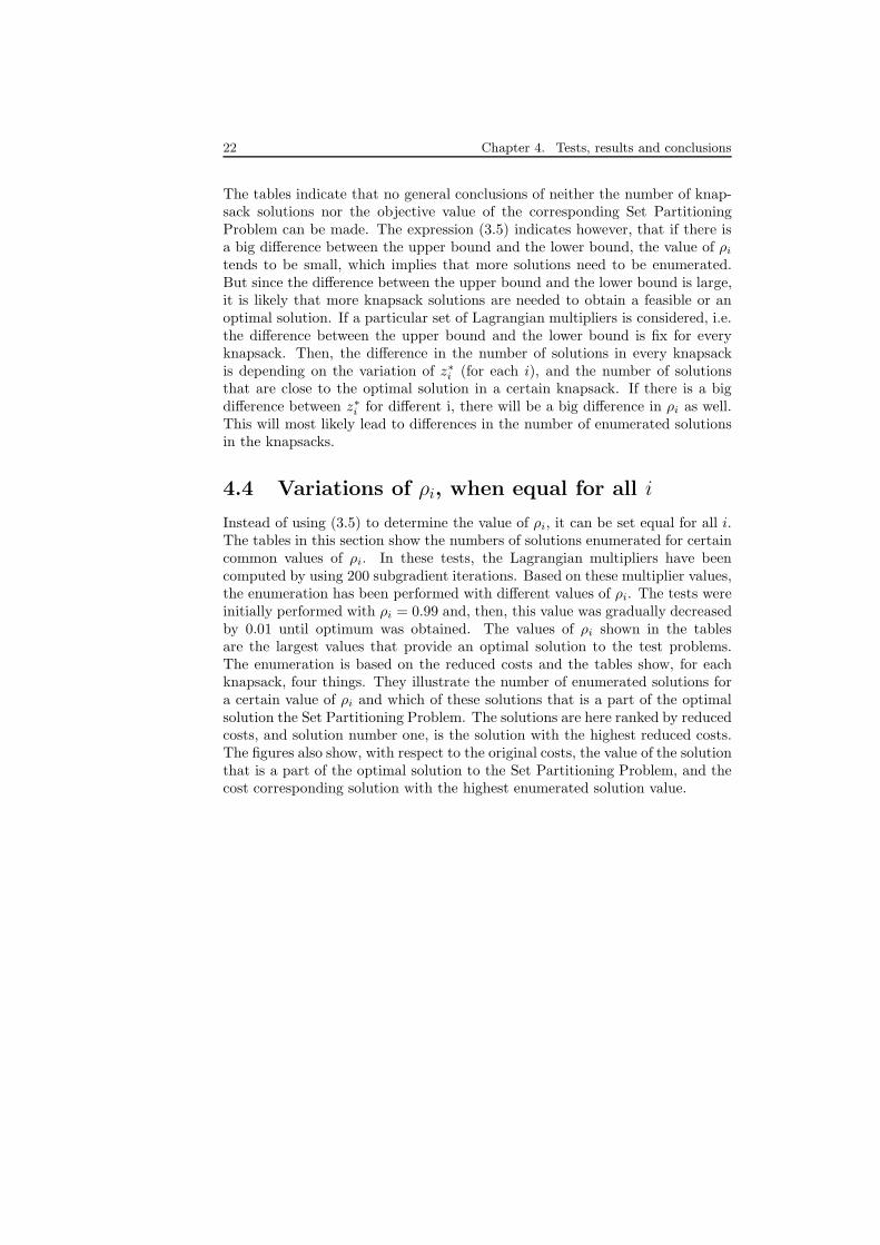
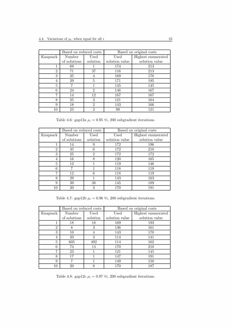
4.4 Variations of ρi, when equal for all i
Instead of using (3.5) to determine the value of ρi, it can be set equal for all i.The tables in this section show the numbers of solutions enumerated for certaincommon values of ρi. In these tests, the Lagrangian multipliers have beencomputed by using 200 subgradient iterations. Based on these multiplier values,the enumeration has been performed with different values of ρi. The tests wereinitially performed with ρi = 0.99 and, then, this value was gradually decreasedby 0.01 until optimum was obtained. The values of ρi shown in the tablesare the largest values that provide an optimal solution to the test problems.The enumeration is based on the reduced costs and the tables show, for eachknapsack, four things. They illustrate the number of enumerated solutions fora certain value of ρi and which of these solutions that is a part of the optimalsolution the Set Partitioning Problem. The solutions are here ranked by reducedcosts, and solution number one, is the solution with the highest reduced costs.The figures also show, with respect to the original costs, the value of the solutionthat is a part of the optimal solution to the Set Partitioning Problem, and thecost corresponding solution with the highest enumerated solution value.
4.4. Variations of ρi, when equal for all i 23
Based on reduced costs Based on original costsKnapsack Number Used Used Highest enumerated
of solutions solution solution value solution value1 69 1 174 2132 71 37 116 2133 35 4 169 1704 29 5 171 1955 7 1 145 1456 24 2 146 1677 14 12 167 1678 25 3 121 1649 18 2 143 166
10 25 2 99 121
Table 4.6: gap12a ρi = 0.95 ∀i, 200 subgradient iterations.
Based on reduced costs Based on original costsKnapsack Number Used Used Highest enumerated
of solutions solution solution value solution value1 14 9 172 1962 35 6 172 2183 25 2 172 1724 16 8 120 1655 12 1 119 1466 7 1 118 1197 12 6 118 1198 29 1 143 1639 39 38 145 189
10 20 3 170 191
Table 4.7: gap12b ρi = 0.96 ∀i, 200 subgradient iterations.
Based on reduced costs Based on original costsKnapsack Number Used Used Highest enumerated
of solutions solution solution value solution value1 18 18 169 1932 8 3 136 1613 10 4 143 1704 33 3 114 1415 605 492 114 1626 74 14 170 2107 23 1 121 1458 17 1 147 1919 7 1 149 150
10 20 8 170 187
Table 4.8: gap12c ρi = 0.97 ∀i, 200 subgradient iterations.
24 Chapter 4. Tests, results and conclusions
Based on reduced costs Based on original costsKnapsack Number Used Used Highest enumerated
of solutions solution solution value solution value1 51 12 144 2112 8 1 150 1503 25 1 173 1744 29 2 146 1875 38 1 122 1226 20 1 140 1637 20 19 143 1668 144 140 141 1999 34 1 145 145
10 8 1 143 143
Table 4.9: gap12d ρi = 0.96 ∀i, 200 subgradient iterations.
Based on reduced costs Based on original costsKnapsack Number Used Used Highest enumerated
of solutions solution solution value solution value1 34 5 149 1722 27 4 162 1863 31 1 143 1644 32 2 169 1715 64 7 171 1926 24 11 147 1657 36 4 170 1948 67 59 93 1409 28 2 123 144
10 9 6 119 145
Table 4.10: gap12e ρi = 0.95 ∀i, 200 subgradient iterations.
4.5. Conclusions and future work 25
In the tests performed in this section, it is in one or two knapsacks, necessaryto enumerate many more solutions to obtain optimality, compared to the otherknapsacks. Note that if a knapsack solution has the highest value with respectto the reduced cost, it does not imply that it has the highest value with respectto the original cost.
4.5 Conclusions and future work
In this thesis, a method for solving the Generalized Assignment Problem hasbeen presented. After applying Lagrangian relaxation the problem separatesinto one knapsack problem for each agent. Then, solutions to the knapsackproblems that arose from the Lagrangian relaxation are enumerated. The nextstep is to choose one solution to every knapsack, and to put these solutions to-gether to form a solution to the original Generalized Assignment Problem. Bychanging the values of different parameters, various test results were obtained.Based on these results, we can draw some preliminary conclusions regarding themethod.
Due to the type of test data used, no general conclusion regarding the methodcan be drawn. The tests indicate, however, that it is worth the effort of comput-ing fairly near-optimal Lagrangian multipliers. Good values of these multipliersyield a smaller number of knapsack solutions that needs to be enumerated. Thetests also indicate that there is no need in computing the value of the parameterρi (the parameter that controls the maximum deviation in the original costs ofthe enumerated knapsack solutions to knapsack i) as in Section 3.5, instead itseems favorable to set ρi equal for all i. One possible reason for the great differ-ence in the number of enumerated solutions when ρi is calculated as in Section3.5, is that |z∗i | (the objective value of the optimal solution to knapsack i, withrespect to Lagrangian reduced costs) in the denominator has greater effect thanexpected. This could be an explanation to the results in Section 4.3.
Since all of the test problems are of the same size and type, a natural proceed-ing of this thesis would be an extension of the test data set. Another possiblesubject for future work is to study the difference between the optimal knapsacksolutions, with respect to their reduced costs. In Section 4.4, one can observe,that there is one or two knapsacks where the solutions used have a significantlower ranking than the solutions used in the other knapsacks. This is an in-teresting observation and it could be a subject for future work (if this is truein more general cases) to, before the enumeration begins, determine in whichknapsacks large numbers of solutions need to be enumerated. Future work canalso include a study of the CPU-time needed to solve the Generalized Assign-ment Problem with this method. This would indicate whether the method isworth further consideration.

26 Chapter 4. Tests, results and conclusions
Bibliography
[1] Martin Savelsbergh, A branch-and-price algorithm for the generalized as-signment problem, Operations Research 45, 1997, 831-841.
[2] David Pisinger, An expanding-core algorithm for the exact 0-1 knapsackproblem, European Journal of Operational Research 87, 1995, 175-187.
[3] Marshall L. Fisher, The Lagrangian relaxation method for solving integerprogramming problems, Management Science 27, 1981, 1-18.
[4] Sartaj Sahni and Teofilo Gonzalez, P-complete approximation problems,Journal of the Association for Computing Machinery 23, 1976, 555-565.
[5] Mutsunori Yagiura, Toshilde Ibaraki and Fred Glover, An ejection chainapproach for the generalized assignment problem, INFORMS Journal onComputing 16, 2004, 131-151.
[6] Asa Revenius, Enumeration of Solutions to the Binary Knapsack Prob-lem, LITH-MATH-EX-2004-07, Master thesis, Department of Mathemat-ics, Linkoping University, Sweden.
[7] Ravindra K. Ahuja, Thomas L. Magnati and James B. Orlin, NetworkFlows, Theory Algorithms and Applications, Percentice-Hall, New Jersey,1993.
[8] Robert M. Nauss, Solving the generalized assignment problem: an optimiz-ing and heuristic approach, INFORMS Journal on Computing 15, 2003,249-266.
[9] Dirk. G. Cattrysse, Marc Salomon and Luk N. Van Wassenhove, A setpartitioning heuristic for the generalized assignment problem, EuropeanJournal of Operational Research 72, 1994, 167-174.
[10] John E. Beasley, http://people.brunel.ac.uk/∼mastjjb/jeb/orlib/gapinfo.html.
[11] Torbjorn Larsson and Michael Patriksson, Global optimality conditionsfor discrete and nonconvex optimization-With applications to Lagrangianheuristics and column generation, Forthcoming in Operations Research.
[12] George. B. Dantzig, Discrete variables extremum problems, Operations Re-search 5, 1957, 266-277.
[13] Niclas Andreasson, Anton Evgrafov and Michael Patriksson, An Intro-duction to Continuous Optimization: Foundations and Fundamental Al-gorithms, Studentlitteratur, 2005.
Brommesson, 2006. 27

28 Bibliography
LINKÖPING UNIVERSITY
ELECTRONIC PRESS
Copyright
The publishers will keep this document online on the Internet - or its possi-ble replacement - for a period of 25 years from the date of publication barringexceptional circumstances. The online availability of the document implies apermanent permission for anyone to read, to download, to print out single copiesfor your own use and to use it unchanged for any non-commercial research andeducational purpose. Subsequent transfers of copyright cannot revoke this per-mission. All other uses of the document are conditional on the consent of thecopyright owner. The publisher has taken technical and administrative mea-sures to assure authenticity, security and accessibility. According to intellectualproperty law the author has the right to be mentioned when his/her work isaccessed as described above and to be protected against infringement. For ad-ditional information about the Linkoping University Electronic Press and itsprocedures for publication and for assurance of document integrity, please referto its WWW home page: http://www.ep.liu.se/
Upphovsratt
Detta dokument halls tillgangligt pa Internet - eller dess framtida ersattare- under 25 ar fran publiceringsdatum under forutsattning att inga extraordi-nara omstandigheter uppstar. Tillgang till dokumentet innebar tillstand forvar och en att lasa, ladda ner, skriva ut enstaka kopior for enskilt bruk ochatt anvanda det oforandrat for ickekommersiell forskning och for undervisning.Overforing av upphovsratten vid en senare tidpunkt kan inte upphava dettatillstand. All annan anvandning av dokumentet kraver upphovsmannens med-givande. For att garantera aktheten, sakerheten och tillgangligheten finns detlosningar av teknisk och administrativ art. Upphovsmannens ideella ratt in-nefattar ratt att bli namnd som upphovsman i den omfattning som god sedkraver vid anvandning av dokumentet pa ovan beskrivna satt samt skydd motatt dokumentet andras eller presenteras i sadan form eller i sadant sammanhangsom ar krankande for upphovsmannens litterara eller konstnarliga anseende elleregenart. For ytterligare information om Linkoping University Electronic Pressse forlagets hemsida http://www.ep.liu.se/
c© 2006, Peter Brommesson
Brommesson, 2006. 29