quadrotor assignment

Modeling and simulation of Quad rotor helicopter using H infinity controllerABSTRACT

This report will present an integral predictive/H infinity control structure design in order to provide a solution for the path following quad rotor helicopter. By utilizing Taylor’s series this work will develop a linearized dynamic equation for the system. Therefore the developed model will be simulated by utilizing Mat lab/Simulink software. The simulation results therefore are to enhance the performance of the proposed control design strategy.

2013

OKOYE CHUKWUNAENYE NNANNA .S.UNIVERSITY OF DERBY

5/29/2013

Modeling and simulation of Quadrotor helicopter using H infinity

controller

2013

ContentsCHAPTER 1............................................................2

INTRODUCTION........................................................2CHAPTER 2............................................................2

STATE OF ART........................................................2CHAPTER 3............................................................4

QUAD ROTOR MODEL AND SYSTEM.........................................43.1 Basic Concepts................................................4

3.2 Newton-Euler model............................................83.3 DC Motor.....................................................11

Voltage and angular velocity of propeller...........................13Voltage and thrust..................................................13

CHAPTER 4...........................................................18CONTROL ALGORITHM..................................................18

4.1 Control modeling.............................................184.2 H infinity controller........................................20

4.3 Quad rotor Simulation........................................234.3 Simulation Results...........................................25

4.4 Discussion...................................................294.5 Conclusion...................................................30

4.6 Reference....................................................304.6 Appendix.....................................................31

1 MSc in Control and Instrumentation

Modeling and simulation of Quad rotor helicopter using H infinity controllerABSTRACT

This report will present an integral predictive/H infinity control structure design in order to provide a solution for the path following quad rotor helicopter. By utilizing Taylor’s series this work will develop a linearized dynamic equation for the system. Therefore the developed model will be simulated by utilizing Mat lab/Simulink software. The simulation results therefore are to enhance the performance of the proposed control design strategy.


controller

2013

CHAPTER 1INTRODUCTIONThe design of unmanned aerial vehicles (UAV’S) have much

advantages especially in control area throughout last decades.

Currently this unmanned aerial vehicle has many applications

which include searching and rescuing operations, military

application, and wildlife protection exploration of building

together with security and inspection task. This UAV are very

important especially when all this applications are being

executed in a most dangerous and unapproachable surroundings or

environments. For the past few years the configuration of UAV in

the quad rotor has been noted in so many articles. This vehicle

mostly relies on vertical take-off and landing concepts which is

also known as VTOL which can be also utilized in the development



controller

2013

of control laws. Moreover in this kind of helicopter it makes use

of the equilibrium forces developed by the four rotors. Therefore

among the advantages of this configured quad rotor is its ability

of load capacity. Mostly this helicopter can be maneuverable i.e.

it can be able to maneuver in different direction which does

enable take-off and landing as well as flight in a rugged

environment. The main aims of this report are the system

modeling, control technique or algorithm, evaluation and

simulation design.

CHAPTER 2STATE OF ARTFor the past few years, the state of the art in vertical take-off

and landing (VTOL) unmanned aerial vehicle has attracted

different contributes. Some project which relies on commercially

available platforms such as Draganflyer, X-UFO and MD4-200. Some

of the researchers instead prefer to develop their own structure.

A few other works directs its attention on modeling derivation



controller

2013

and efficient configuration. The most important techniques and

the respective publication are now presented:

The first control is done using Lyapunov theory.

The second control is provided by PD2 feedback and PID structure.

On the contrary a PID structure does not require some specific

model parameters and the control law is much simpler to

implement.

The third control uses an adaptive technique.

While fourth control is based on linear quadratic regulator (LQR)

the main advantage of this technique is that the optimal input

signals turn out to be obtained from full state feedback by

solving the Ricatti equation.

The fifth control is done with back stepping control technique.

The sixth control is provided by dynamic feedback.

CHAPTER 34 MSc in Control and Instrumentation


controller

2013

QUAD ROTOR MODEL AND SYSTEMConsidering this chapter, the quad rotor models are derived. The

result is indeed crucial due to the movement of the helicopter

with respect to its inputs. Therefore through the equation it

makes it easy to predict the position acquired by the helicopter

by observing its motor speed.

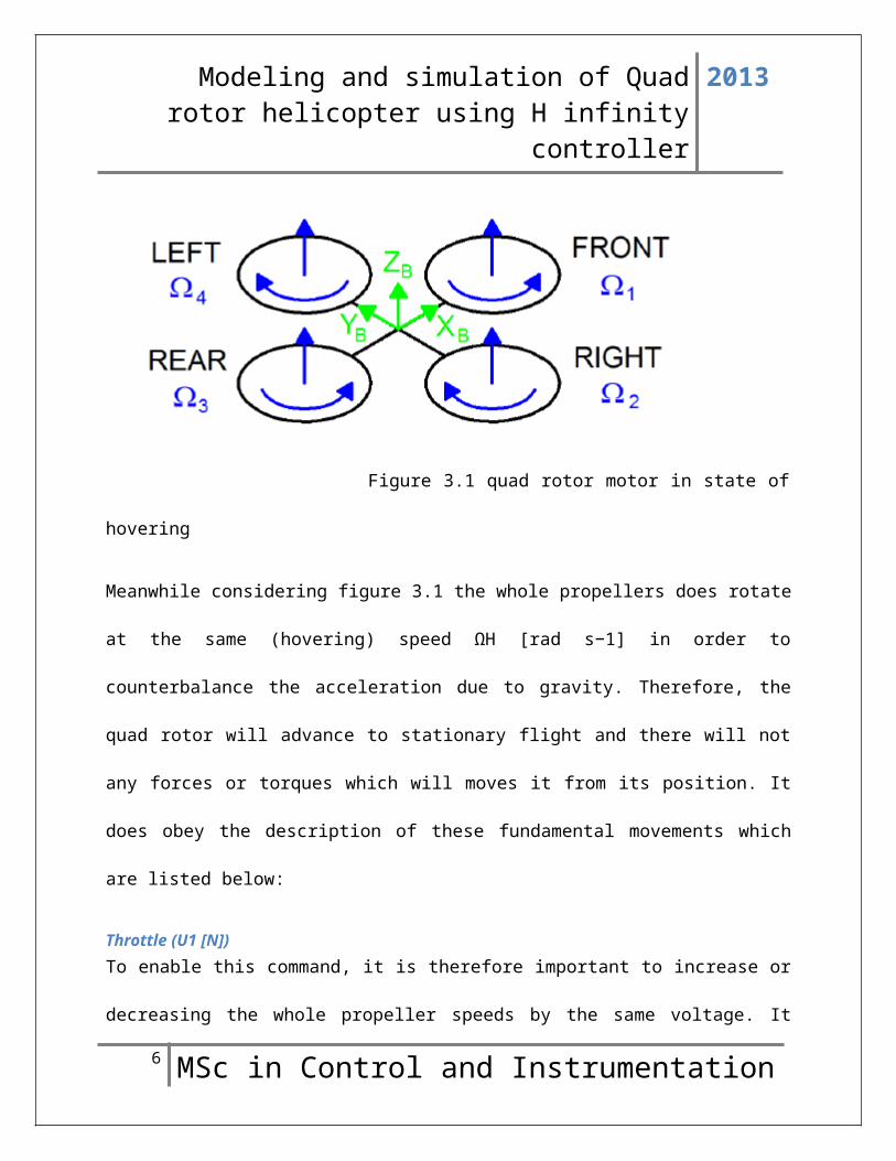
3.1 Basic ConceptsA quad rotor can be said to be a model which consist of four

rotors in a cross configuration position. Concerning the cross

configuration it physical structure is light and thin, therefore

it displays robustness by connecting the motors mechanically.

While rotating the front and rear propellers rotate counter clock

wise, while both the left and right movies in clock wise

direction. Due to this configuration it does eliminate the

requirement for a tail rotor. The diagram below displays the

physical structure model in the state of hovering, where by all

the propeller has equal speed.



controller

2013

Figure 3.1 quad rotor motor in state of

hovering

Meanwhile considering figure 3.1 the whole propellers does rotate

at the same (hovering) speed ΩH [rad s−1] in order to

counterbalance the acceleration due to gravity. Therefore, the

quad rotor will advance to stationary flight and there will not

any forces or torques which will moves it from its position. It

does obey the description of these fundamental movements which

are listed below:

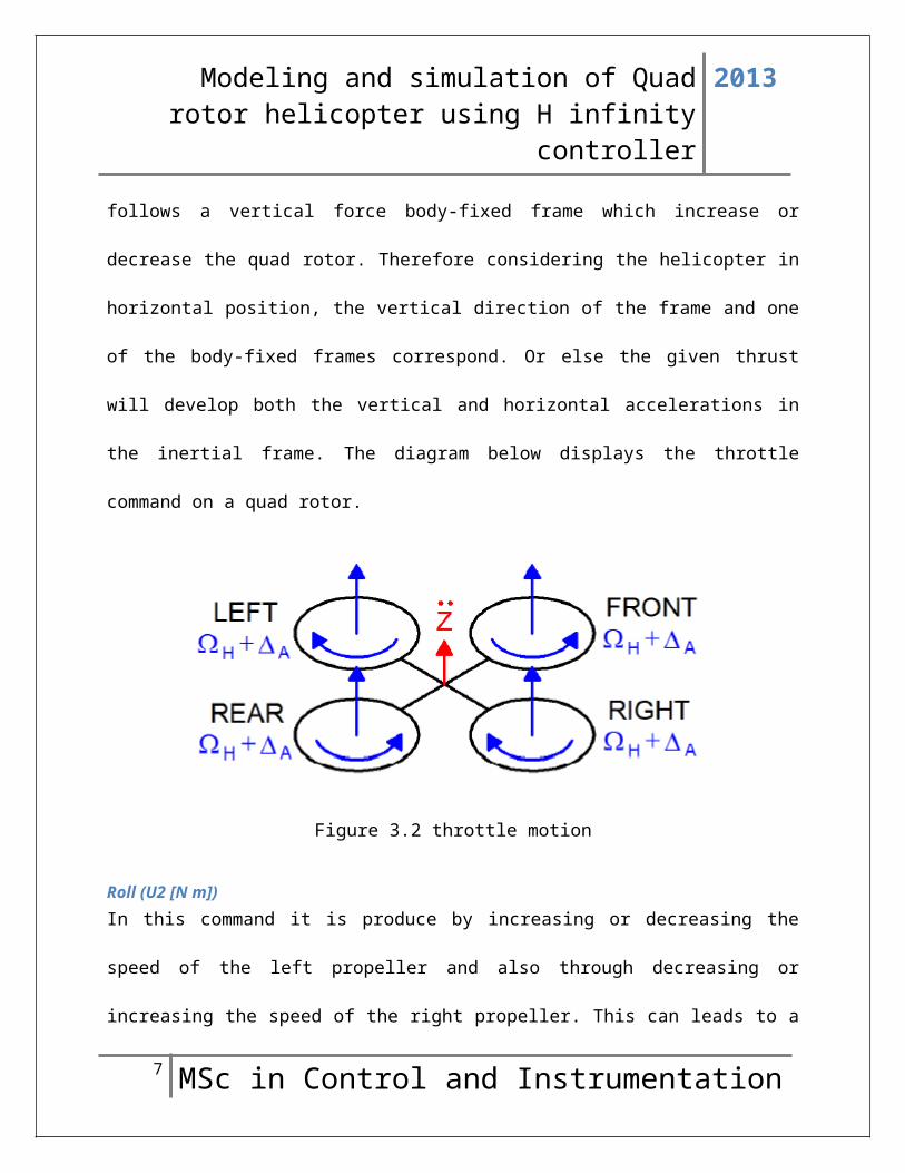
Throttle (U1 [N])To enable this command, it is therefore important to increase or

decreasing the whole propeller speeds by the same voltage. It



controller

2013

follows a vertical force body-fixed frame which increase or

decrease the quad rotor. Therefore considering the helicopter in

horizontal position, the vertical direction of the frame and one

of the body-fixed frames correspond. Or else the given thrust

will develop both the vertical and horizontal accelerations in

the inertial frame. The diagram below displays the throttle

command on a quad rotor.

Figure 3.2 throttle motion

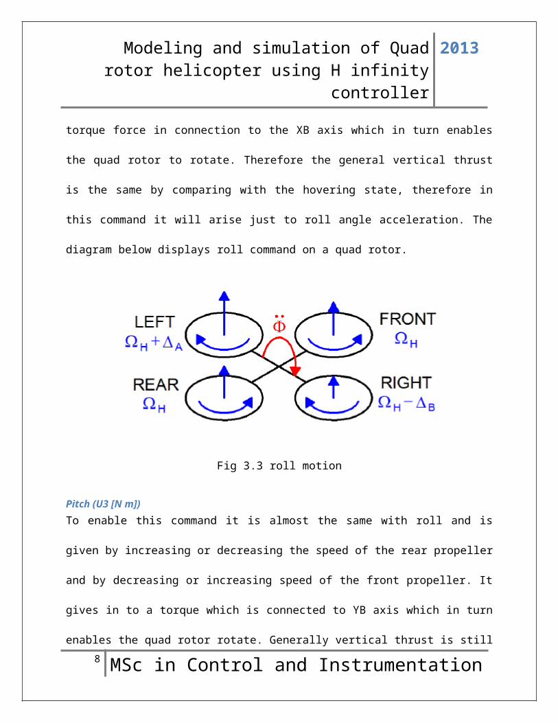
Roll (U2 [N m])In this command it is produce by increasing or decreasing the

speed of the left propeller and also through decreasing or

increasing the speed of the right propeller. This can leads to a



controller

2013

torque force in connection to the XB axis which in turn enables

the quad rotor to rotate. Therefore the general vertical thrust

is the same by comparing with the hovering state, therefore in

this command it will arise just to roll angle acceleration. The

diagram below displays roll command on a quad rotor.

Fig 3.3 roll motion

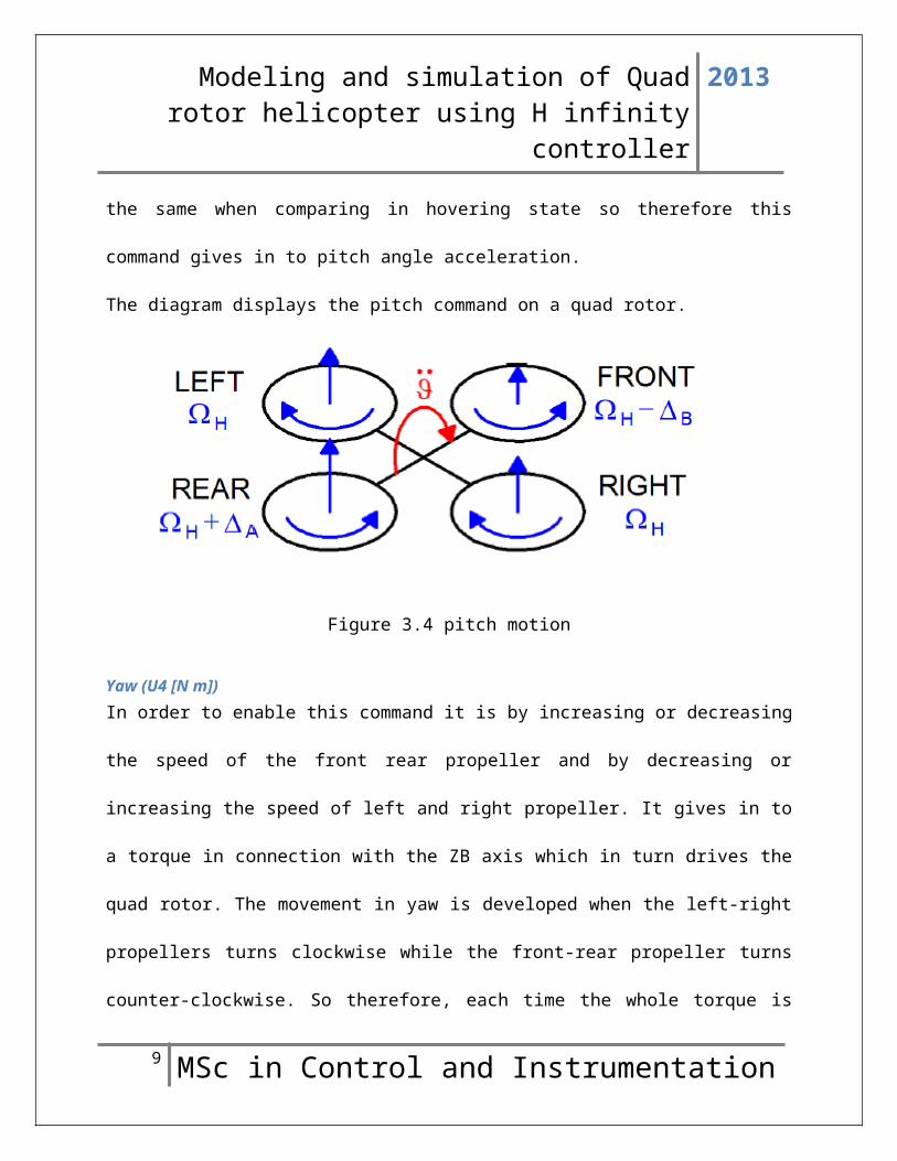
Pitch (U3 [N m])To enable this command it is almost the same with roll and is

given by increasing or decreasing the speed of the rear propeller

and by decreasing or increasing speed of the front propeller. It

gives in to a torque which is connected to YB axis which in turn

enables the quad rotor rotate. Generally vertical thrust is still8 MSc in Control and Instrumentation


controller

2013

the same when comparing in hovering state so therefore this

command gives in to pitch angle acceleration.

The diagram displays the pitch command on a quad rotor.

Figure 3.4 pitch motion

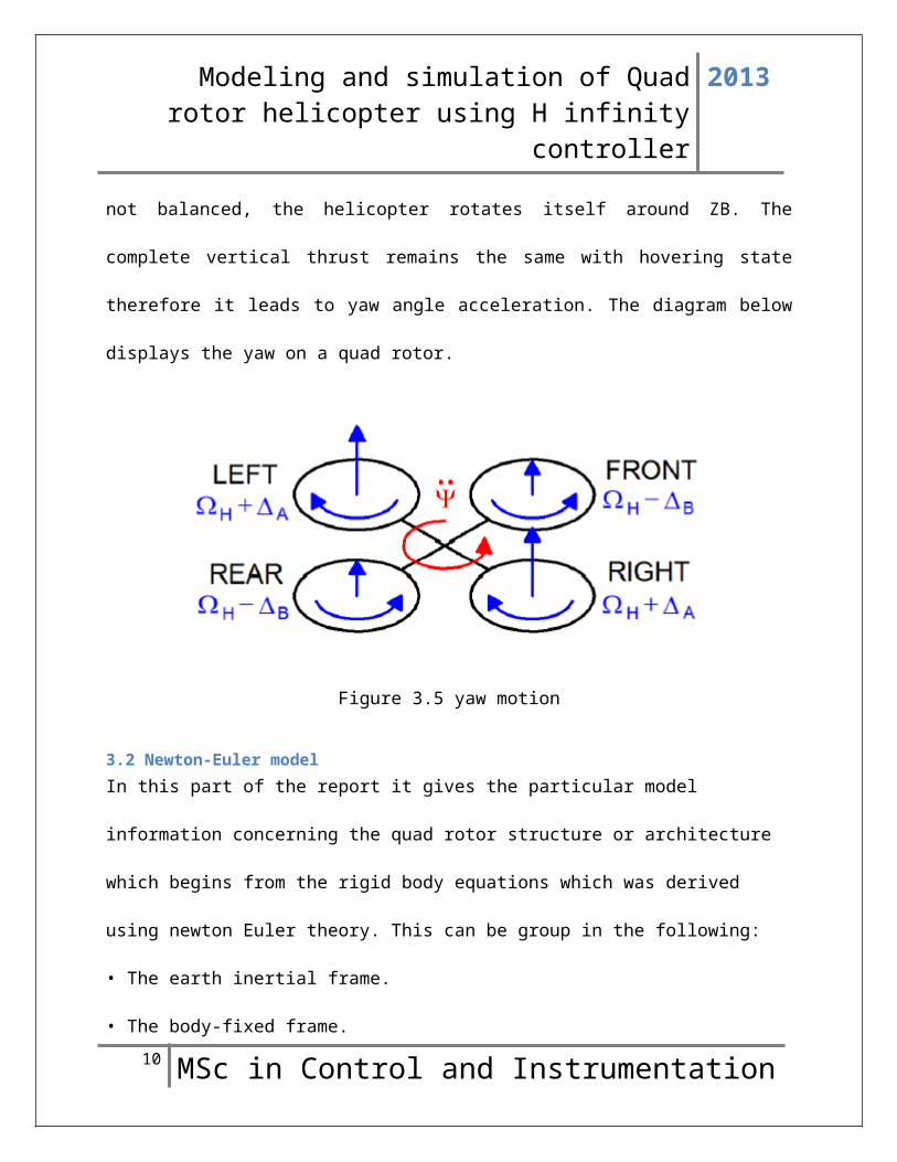
Yaw (U4 [N m])In order to enable this command it is by increasing or decreasing

the speed of the front rear propeller and by decreasing or

increasing the speed of left and right propeller. It gives in to

a torque in connection with the ZB axis which in turn drives the

quad rotor. The movement in yaw is developed when the left-right

propellers turns clockwise while the front-rear propeller turns

counter-clockwise. So therefore, each time the whole torque is



controller

2013

not balanced, the helicopter rotates itself around ZB. The

complete vertical thrust remains the same with hovering state

therefore it leads to yaw angle acceleration. The diagram below

displays the yaw on a quad rotor.

Figure 3.5 yaw motion

3.2 Newton-Euler modelIn this part of the report it gives the particular model

information concerning the quad rotor structure or architecture

which begins from the rigid body equations which was derived

using newton Euler theory. This can be group in the following:

• The earth inertial frame.

• The body-fixed frame.10 MSc in Control and Instrumentation


controller

2013

• The inertia matrix is time-invariant.

The motion equation is more easily created in the body-fixed

frame due to some certain reasons:

• The body symmetry can be assumed to analyze the equations.

Equation (3.1) explains the kinematics of a rigid-body.

ᶓ = JӨ V ---------------------------------------- (3.1)

Where by ᶓ is the velocity vector E-frame, V is the velocity

vector B-frame and JӨ is the generalized matrix.

ᶓ is composed of the quad rotor linear ᴦE [m] and angular ΘE

[rad] position vectors-frame as shown in equation (3.2)

ᶓ=¿ ------------------------- (3.2)

Similarly is composed of the quad rotor linear VB [m s−1] and

angular ῳB [rad s−1] velocity vectors WRT B-frame as shown in

equation (3.3)

V=¿ ---------------------------- (3.3)

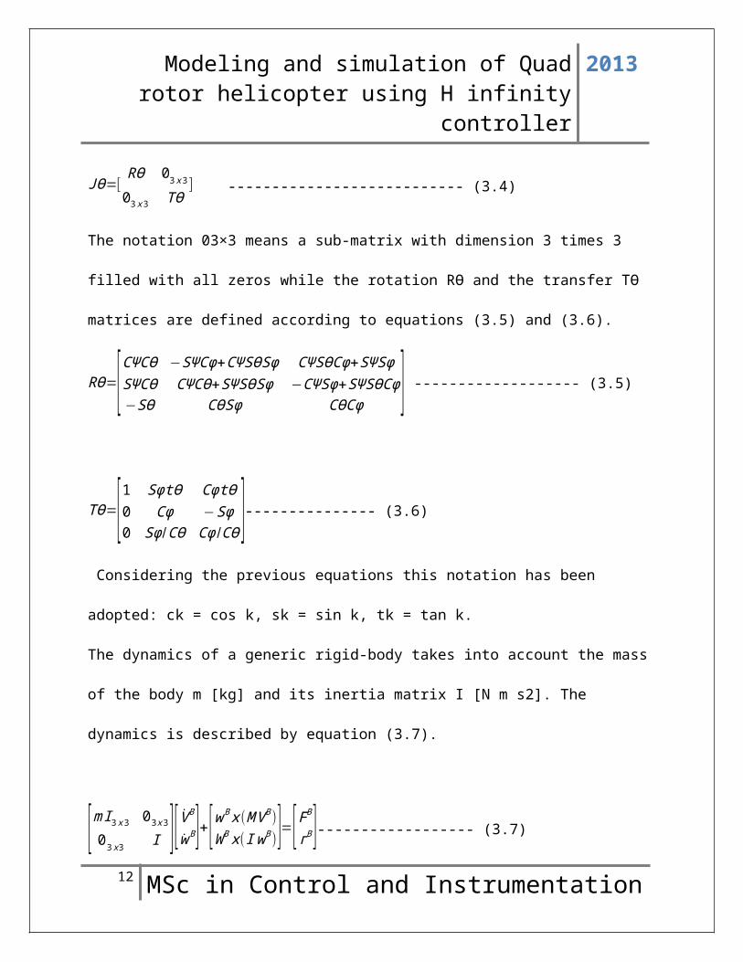
In addition, the generalized matrix JӨ is composed of 4 sub-matrixes according to equation (3.4).



controller

2013

JӨ=[RӨ 03x303x3 TӨ

] --------------------------- (3.4)

The notation 03×3 means a sub-matrix with dimension 3 times 3

filled with all zeros while the rotation RӨ and the transfer TӨ

matrices are defined according to equations (3.5) and (3.6).

RӨ=[CΨCӨ −SΨCϕ+CΨSӨSϕ CΨSӨCϕ+SΨSϕSΨCӨ CΨCӨ+SΨSӨSϕ −CΨSϕ+SΨSӨCϕ−SӨ CӨSϕ CӨCϕ ] ------------------- (3.5)

TӨ=[1 SϕtӨ CϕtӨ0 Cϕ −Sϕ0 Sϕ/CӨ Cϕ /CӨ ]--------------- (3.6)

Considering the previous equations this notation has been

adopted: ck = cos k, sk = sin k, tk = tan k.

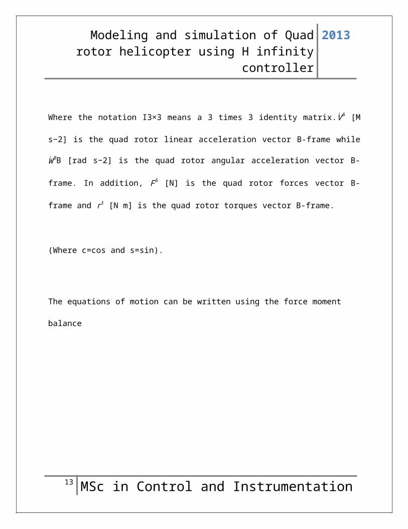
The dynamics of a generic rigid-body takes into account the mass

of the body m [kg] and its inertia matrix I [N m s2]. The

dynamics is described by equation (3.7).

[mI3x3 03x3

03x3 I ][VB

wB]+[wBx(MVB)WBx(IwB)]=[FBᴦB]------------------ (3.7)



controller

2013

Where the notation I3×3 means a 3 times 3 identity matrix.VB [M

s−2] is the quad rotor linear acceleration vector B-frame while

WBB [rad s−2] is the quad rotor angular acceleration vector B-

frame. In addition, FB [N] is the quad rotor forces vector B-

frame and ᴦB [N m] is the quad rotor torques vector B-frame.

(Where c=cos and s=sin).

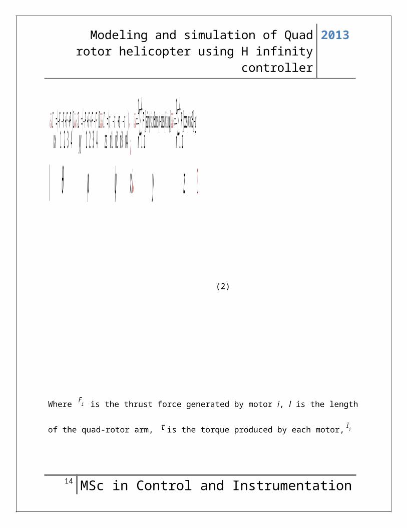
The equations of motion can be written using the force moment

balance



controller

2013

| θ¿⋅¿I

xx=(−F

1−F

2+F3

+F4)l ¿

ϕ¿⋅¿I

yy=(−F

1+F2+F3

−F4

)l ¿

ψ¿⋅¿I

zz=(τ

m1−τ

m2+τm3

−τm4

)¿

x¿

¿ y¿⋅¿=1

m∑14F

i[sinψsinθcosϕ−cosψsin ϕ] ¿

z¿⋅¿=1

m∑14 F

i[cos ϕcosθ ]−g

¿

(2)

Where Fi is the thrust force generated by motor i, l is the length

of the quad-rotor arm, τ is the torque produced by each motor, Ii



controller

2013

’s the moments of inertia with respect to the axes and m the mass

of the helicopter.

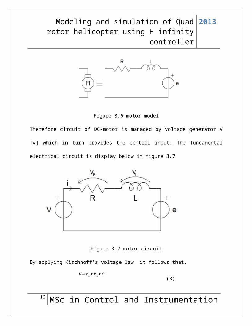
3.3 DC MotorThe DC-motor can be defined as an actuator which therefore

converts electrical energy into mechanical energy. It comprises

of two circuits which are electromagnetic in nature. Therefore

the first is known as rotor which moves around in seconds while

the other is known as stator which does not move. Through the

application DC-current flow in windings, the rotor rotates due to

the force develop through electrical and magnetic reactions.

Moreover the model comprises of resistor R [Ω] in series,

inductor L [H] together with a voltage generator e [V]. Finally

the voltage supplies a voltage which is proportional to the speed

of motor. The model is displays in figure 3.6



controller

2013

Figure 3.6 motor model

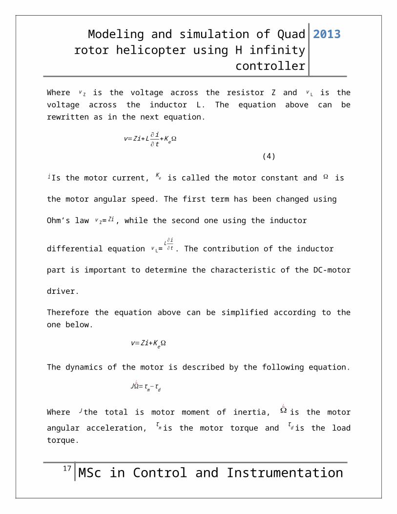
Therefore circuit of DC-motor is managed by voltage generator V

[v] which in turn provides the control input. The fundamental

electrical circuit is display below in figure 3.7

Figure 3.7 motor circuit

By applying Kirchhoff’s voltage law, it follows that.

v=vZ+vL+e (3)



controller

2013

Where v Z is the voltage across the resistor Z and v L is thevoltage across the inductor L. The equation above can berewritten as in the next equation.

v=Zi+L ∂i∂t

+KeΩ

(4)

iIs the motor current, Ke is called the motor constant and Ω is

the motor angular speed. The first term has been changed using

Ohm’s law v Z= Zi , while the second one using the inductor

differential equation v L=L ∂i

∂t . The contribution of the inductor

part is important to determine the characteristic of the DC-motor

driver.

Therefore the equation above can be simplified according to theone below.

v=Zi+KeΩ

The dynamics of the motor is described by the following equation.

JΩ¿=τm−τd

Where J the total is motor moment of inertia, Ω¿

is the motor

angular acceleration, τm is the motor torque and τd is the loadtorque.



controller

2013

Voltage and angular velocity of propeller

Since the voltage inputs V to motors affect the rotational speedΩ of propellers.

V−e=iZ

The dynamics of the motor is described by the following equation

τm−τd=JΩ¿

(8)

Equation (8) states that when the motor torque τm and the drag

torque τd are not equal there is an acceleration (ordeceleration). The back electromotive-force voltage isproportional to motor speed

e=KeΩ (9)

The motor torque is proportional to the field current

τm=Kqi (10)

On substituting, we get

V=τdZKq

+ZJΩ

¿

Kq+KeΩ

(11)

As stated earlier, the drag torque is proportional to the squareof propeller’s speed

τd=DΩ2(12)

The relationship between angular velocity and voltage as found in[51] and [5] can thus be obtained as



controller

2013

V=ZDΩ2

Kq+ZJΩ

¿

Kq+KeΩ

(13)

Voltage and thrust

Voltage is the input of the quad-rotor plant and each rotorproduces a thrust force as it turns. The motor torque is known tobe proportional to the field current

τm=Kqi (14)

τmKq

=i(15)

The electrical power according to Joule’s law is

P=IV=τmKq

V(16)

And the mechanical power output is given as

Pm=ηP=ητmKq

V(17)

With η as the motor efficiency.

The propeller’s figure of merit f is defined as the ratio of

the induced power in air Ph to the mechanical power Pm [2].

f=PhPm (18)

Where Ph is given by

Ph=ηfτmKq

V(19)



controller

2013

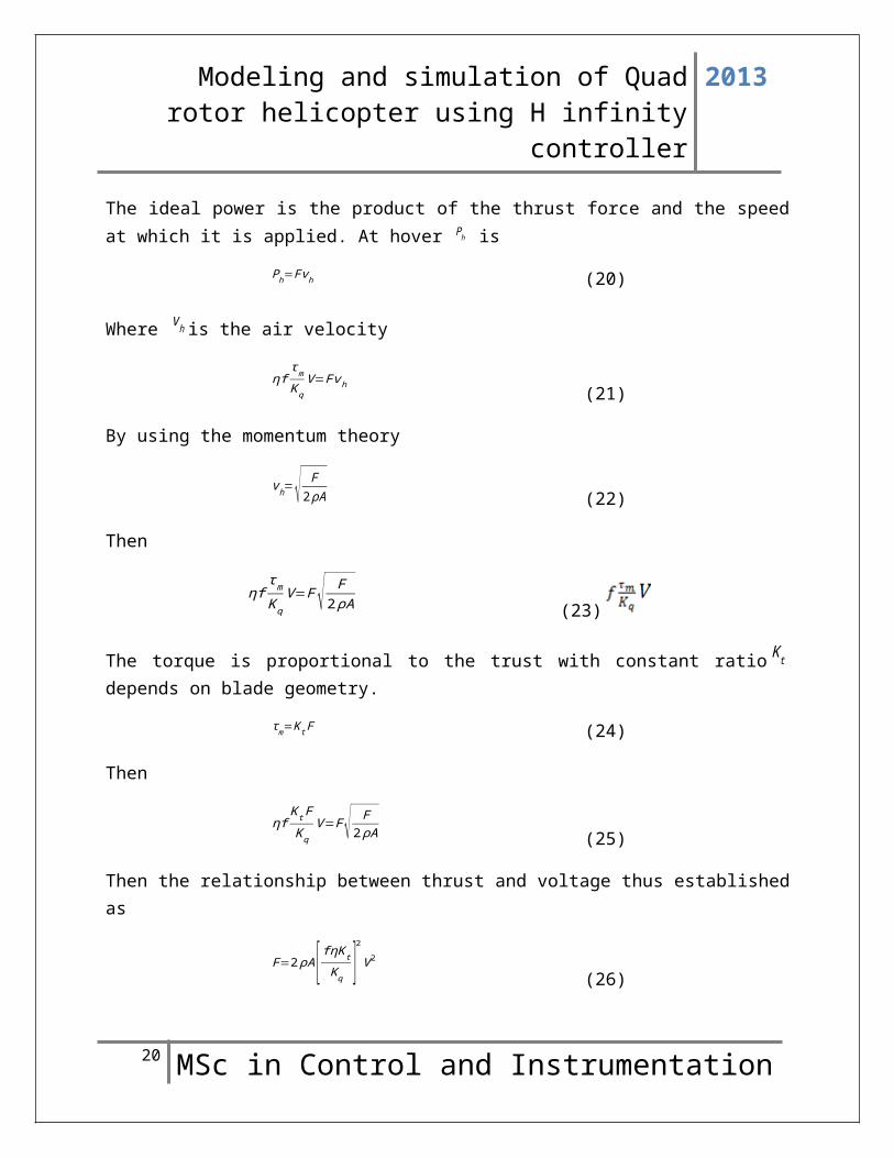
The ideal power is the product of the thrust force and the speedat which it is applied. At hover Ph is

Ph=Fvh (20)

Where vh is the air velocity

ηfτmKq

V=Fvh (21)

By using the momentum theory

vh=√ F2ρA (22)

Then

ηfτmKq

V=F√ F2ρA (23)

The torque is proportional to the trust with constant ratio Ktdepends on blade geometry.

τm=KtF (24)

Then

ηfKtFKq

V=F√ F2ρA (25)

Then the relationship between thrust and voltage thus establishedas

F=2ρA [fηKtKq ]2

V2

(26)



controller

2013

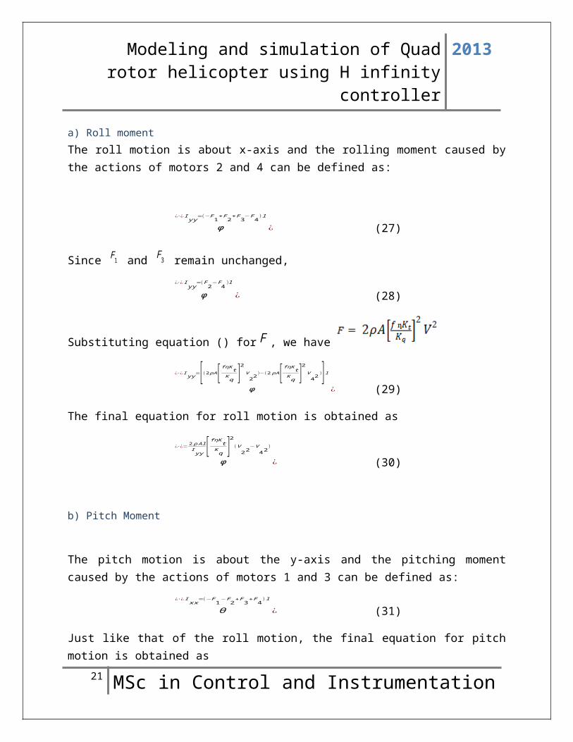
a) Roll momentThe roll motion is about x-axis and the rolling moment caused bythe actions of motors 2 and 4 can be defined as:

ϕ¿⋅¿Iyy=(−F

1+F2

+F3−F

4)l

¿ (27)

Since F1 and F3 remain unchanged,

ϕ¿⋅¿I

yy=(F

2−F

4)l

¿ (28)

Substituting equation () for F , we have

ϕ

¿⋅¿Iyy=[(2ρA[fηKtKq ]2V22

)−(2ρA[fηKtKq ]2V42

)]l¿ (29)

The final equation for roll motion is obtained as

ϕ

¿⋅¿=2ρAlIyy [fηKtKq ]

2(V22

−V42

)

¿ (30)

b) Pitch Moment

The pitch motion is about the y-axis and the pitching momentcaused by the actions of motors 1 and 3 can be defined as:

θ¿⋅¿Ixx=(−F

1−F

2+F3

+F4

)l

¿ (31)

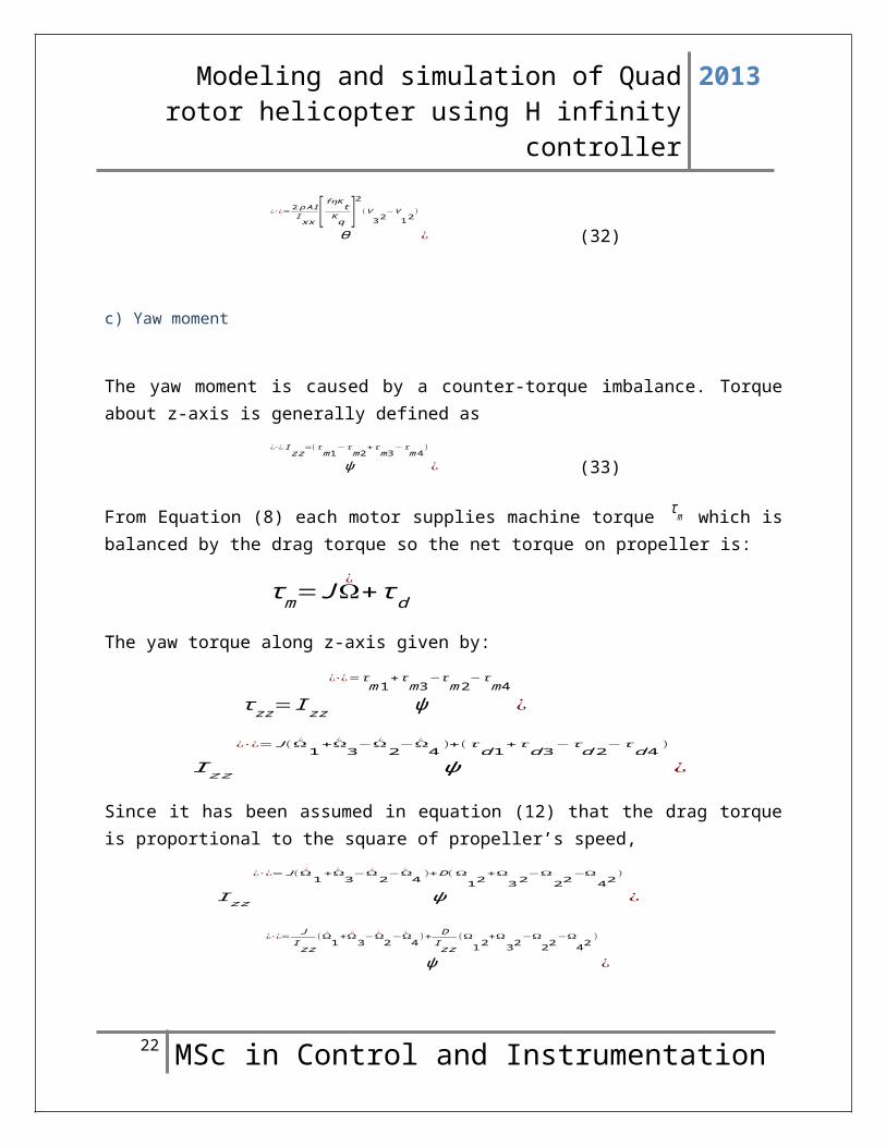
Just like that of the roll motion, the final equation for pitchmotion is obtained as



controller

2013

θ

¿⋅¿=2ρAlIxx [fηKtKq ]

2(V32

−V12

)

¿ (32)

c) Yaw moment

The yaw moment is caused by a counter-torque imbalance. Torqueabout z-axis is generally defined as

ψ¿⋅¿Izz=(τm1−τm2+τm3−τm4)

¿ (33)

From Equation (8) each motor supplies machine torque τm which isbalanced by the drag torque so the net torque on propeller is:

τm=JΩ¿+τd

The yaw torque along z-axis given by:

τzz=Izz ψ¿⋅¿=τm1+τm3−τm2−τm4

¿

Izz ψ¿⋅¿=J(Ω

¿

1+Ω

¿

3−Ω

¿

2−Ω

¿

4)+(τd1+τd3−τd2−τd4 )

¿

Since it has been assumed in equation (12) that the drag torqueis proportional to the square of propeller’s speed,

Izz ψ¿⋅¿=J(Ω

¿

1+Ω

¿

3−Ω

¿

2−Ω

¿

4)+D( Ω

12+Ω

32−Ω

22−Ω

42)

¿

ψ

¿⋅¿= JIzz

(Ω¿

1+Ω

¿

3−Ω

¿

2−Ω

¿

4)+

DIzz

(Ω

12+Ω

32−Ω

22−Ω

42)

¿



controller

2013

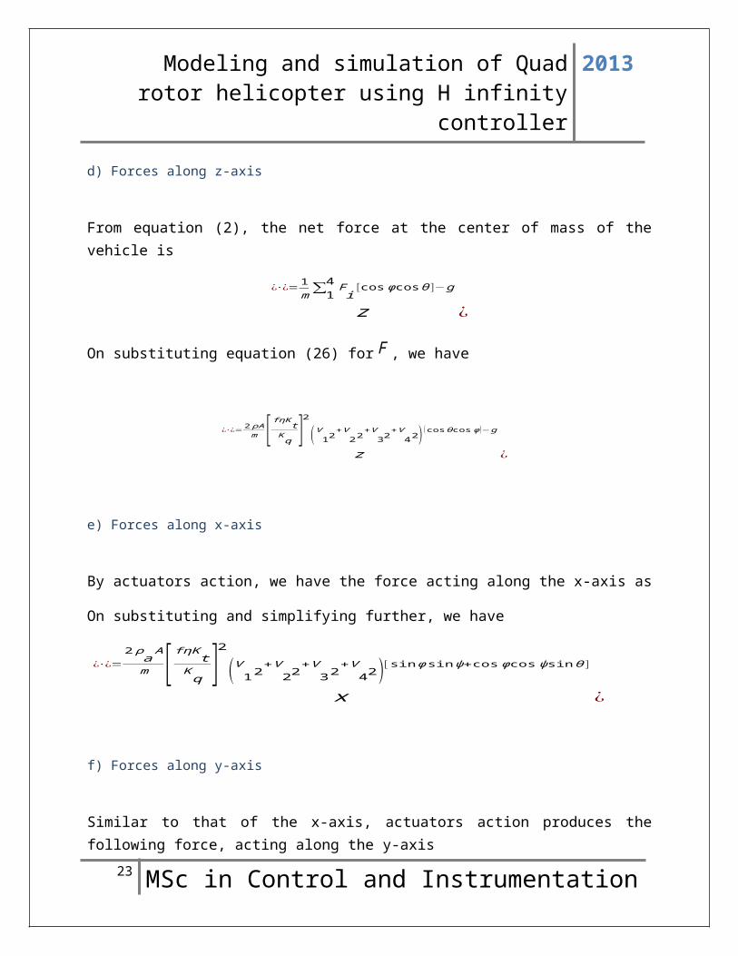
d) Forces along z-axis

From equation (2), the net force at the center of mass of thevehicle is

z¿⋅¿=1

m∑14 Fi [cos ϕcosθ ]−g

¿

On substituting equation (26) for F , we have

z

¿⋅¿=2ρAm [fηKtKq ]

2

(V12+V22

+V32

+V42) (cosθcos ϕ)−g

¿

e) Forces along x-axis

By actuators action, we have the force acting along the x-axis as

On substituting and simplifying further, we have

x

¿⋅¿=2ρaAm [fηKtKq ]

2

(V12+V22

+V32

+V42)[sinϕsinψ+cosϕcos ψsinθ ]

¿

f) Forces along y-axis

Similar to that of the x-axis, actuators action produces thefollowing force, acting along the y-axis



controller

2013

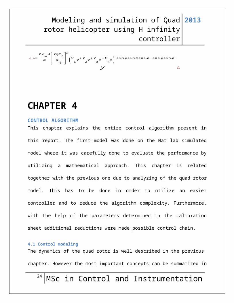
y


2

(V12+V22

+V32

+V42)[sinψsinθcosϕ−cosψsinϕ ]

¿

CHAPTER 4CONTROL ALGORITHMThis chapter explains the entire control algorithm present in

this report. The first model was done on the Mat lab simulated

model where it was carefully done to evaluate the performance by

utilizing a mathematical approach. This chapter is related

together with the previous one due to analyzing of the quad rotor

model. This has to be done in order to utilize an easier

controller and to reduce the algorithm complexity. Furthermore,

with the help of the parameters determined in the calibration

sheet additional reductions were made possible control chain.

4.1 Control modelingThe dynamics of the quad rotor is well described in the previous

chapter. However the most important concepts can be summarized in



controller

2013

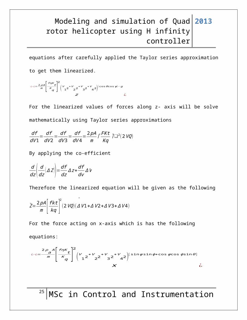
equations after carefully applied the Taylor series approximation

to get them linearized.

z

¿⋅¿=2ρAm [fηKtKq ]

2

(V12+V22

+V32

+V42) (cosθcos ϕ)−g

¿

For the linearized values of forces along z- axis will be solve

mathematically using Taylor series approximations

dfdV1

=dfdV2

=dfdV3

=dfdV 4

=2pAm

⌈FKtKq

⌉2(2VQ)

By applying the co-efficient

ddz ( ddz (∆Z ))=df

dz∆z+

dfdv

∆V

Therefore the linearized equation will be given as the following

¨Z=

2pAm [fktkq ]

2

(2VQ)(∆V1+∆ V2+∆V3+∆V4)

For the force acting on x-axis which is has the following

equations:

x


2

(V12+V22

+V32

+V42)[sinϕsinψ+cos ϕcos ψsinθ ]

¿



controller

2013

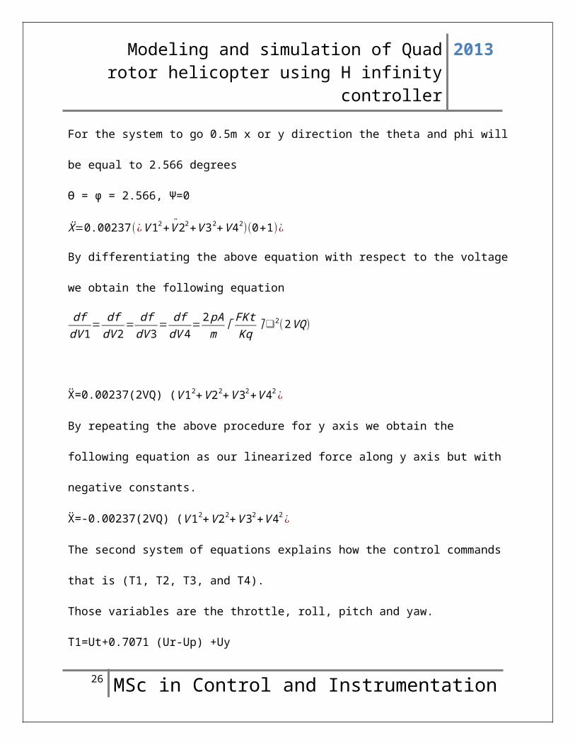
For the system to go 0.5m x or y direction the theta and phi will

be equal to 2.566 degrees

Ө = ϕ = 2.566, Ψ=0

¨Ẍ=0.00237(¿V12+V22+V32+V42)(0+1)¿

By differentiating the above equation with respect to the voltage

we obtain the following equation

dfdV1

=dfdV2

=dfdV3

=dfdV 4

=2pAm

⌈FKtKq

⌉2(2VQ)

Ẍ=0.00237(2VQ) (V12+V22+V32+V42 ¿

By repeating the above procedure for y axis we obtain the

following equation as our linearized force along y axis but with

negative constants.

Ẍ=-0.00237(2VQ) (V12+V22+V32+V42 ¿

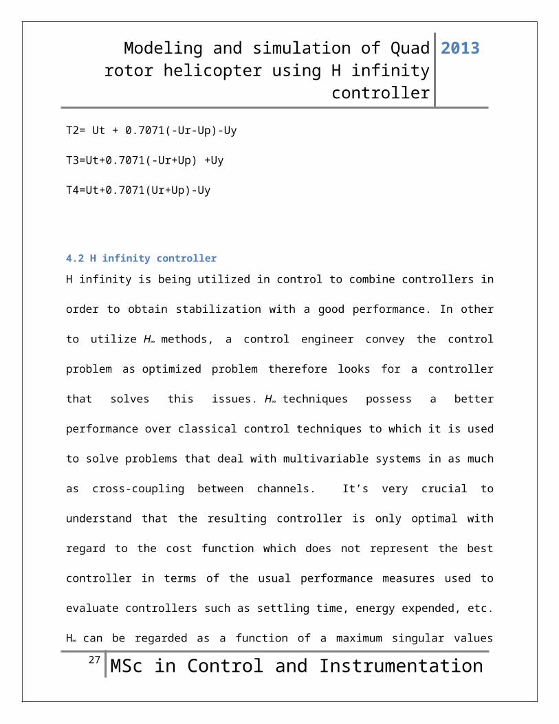
The second system of equations explains how the control commands

that is (T1, T2, T3, and T4).

Those variables are the throttle, roll, pitch and yaw.

T1=Ut+0.7071 (Ur-Up) +Uy



controller

2013

T2= Ut + 0.7071(-Ur-Up)-Uy

T3=Ut+0.7071(-Ur+Up) +Uy

T4=Ut+0.7071(Ur+Up)-Uy

4.2 H infinity controller

H infinity is being utilized in control to combine controllers in

order to obtain stabilization with a good performance. In other

to utilize H∞ methods, a control engineer convey the control

problem as optimized problem therefore looks for a controller

that solves this issues. H∞ techniques possess a better

performance over classical control techniques to which it is used

to solve problems that deal with multivariable systems in as much

as cross-coupling between channels. It’s very crucial to

understand that the resulting controller is only optimal with

regard to the cost function which does not represent the best

controller in terms of the usual performance measures used to

evaluate controllers such as settling time, energy expended, etc.

H∞ can be regarded as a function of a maximum singular values27 MSc in Control and Instrumentation


controller

2013

over a space. (This can be described as a total gain in every

direction and at some frequency, considering SISO systems; this

is efficiently the total magnitude of the frequency

response.). H∞ techniques can equally be used to reduce the

closed loop effect of a perturbation, which does depending on the

problem formulation; the effect will be obtained in terms of

stabilization or performance.

It can be derived by dissolving Riccati’s two equations.

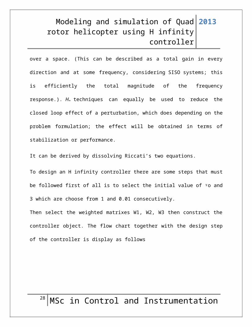
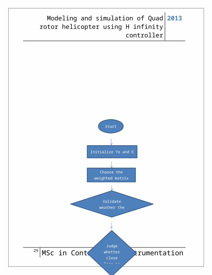
To design an H infinity controller there are some steps that must

be followed first of all is to select the initial value of ᵞo and

З which are choose from 1 and 0.01 consecutively.

Then select the weighted matrixes W1, W2, W3 then construct the

controller object. The flow chart together with the design step

of the controller is display as follows



controller

2013


Start

Initialize ϒo and Є

Choose theweighted matrix

Validateweather the

Judgewhetterclose

loop is


controller

2013

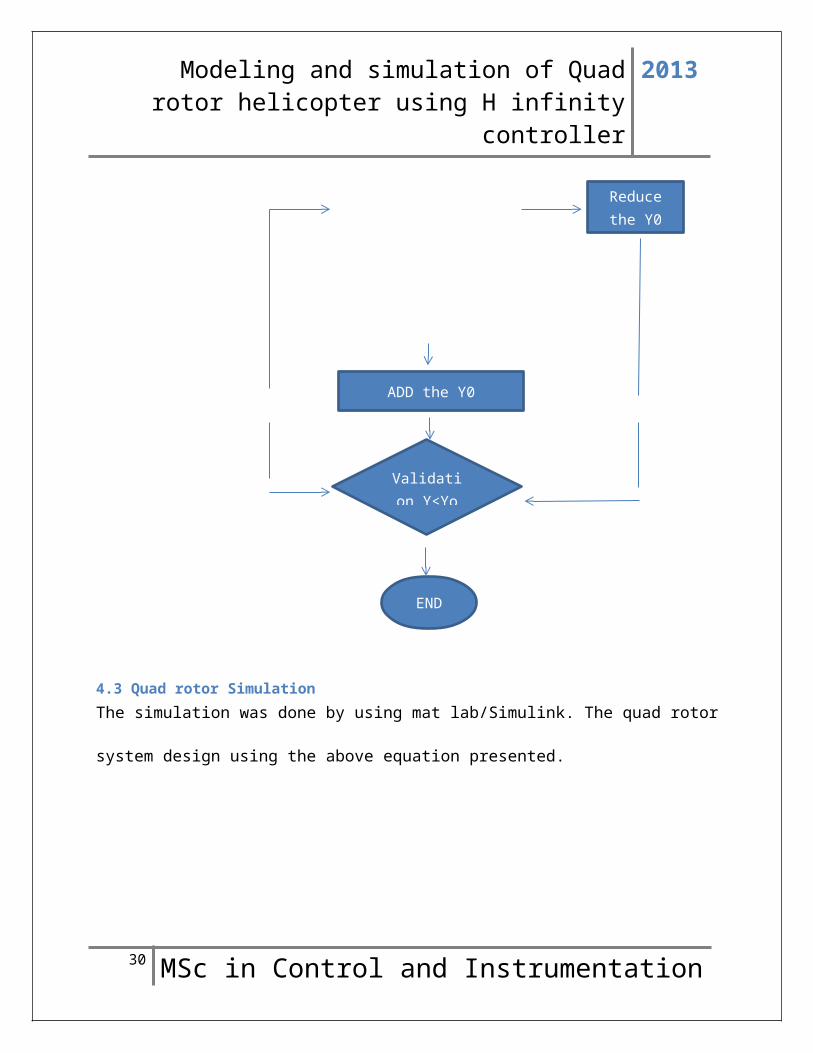
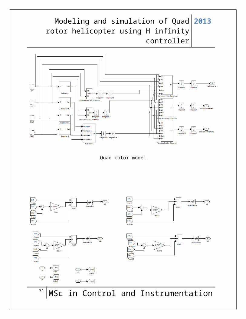
4.3 Quad rotor SimulationThe simulation was done by using mat lab/Simulink. The quad rotor

system design using the above equation presented.


Validation ϒ<ϒo

ADD the ϒ0

END

Reducethe ϒ0


controller

2013

Quad rotor model



controller

2013

Motor Mixing model

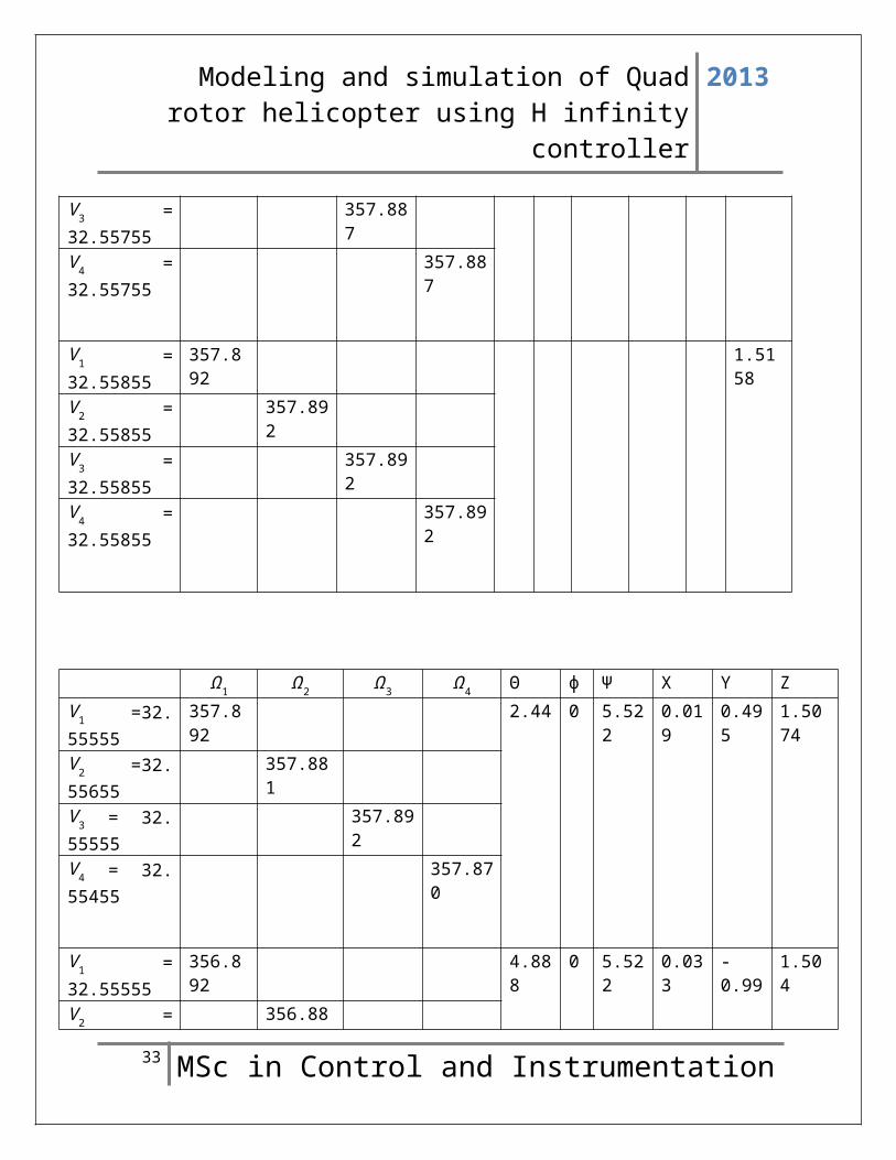
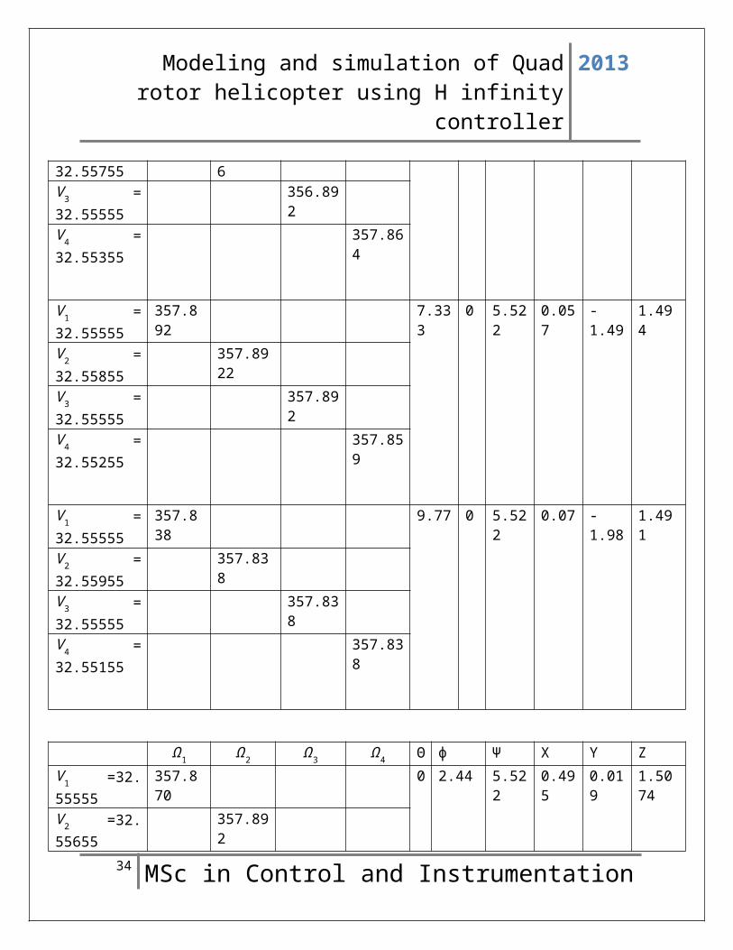
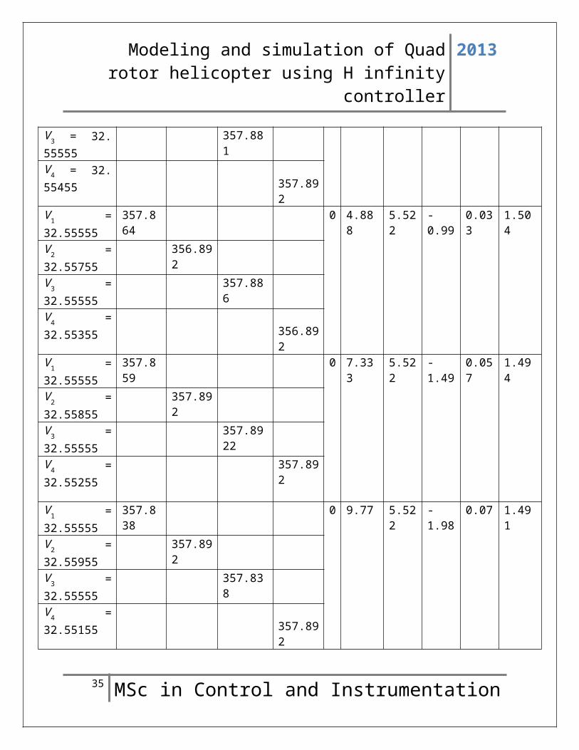
4.3 Simulation Results

Vertical movement In order to attain a particular height, all the voltage inputswere varied at the same rate.

Ω1 Ω2 Ω3 Ω4 Θ ɸ Ψ X Y ZV1 =32.55555

357.876

1.5010

V2 =32.55555

357.876

V3 = 32.55555

357.876

V4 = 32.55555

357.876

V1 =32.55655

356.831

1.5059

V2 =32.55655

356.831

V3 =32.55655

356.831

V4 =32.55655

356.831

V1 =32.55755

357.887

1.5109

V2 =32.55755

357.887



controller

2013

V3 =32.55755

357.887

V4 =32.55755

357.887

V1 =32.55855

357.892

1.5158

V2 =32.55855

357.892

V3 =32.55855

357.892

V4 =32.55855

357.892

Ω1 Ω2 Ω3 Ω4 Θ ɸ Ψ X Y ZV1 =32.55555

357.892

2.44 0 5.522

0.019

0.495

1.5074

V2 =32.55655

357.881

V3 = 32.55555

357.892

V4 = 32.55455

357.870

V1 =32.55555

356.892

4.888

0 5.522

0.033

-0.99

1.504

V2 = 356.88



controller

2013

32.55755 6V3 =32.55555

356.892

V4 =32.55355

357.864

V1 =32.55555

357.892

7.333

0 5.522

0.057

-1.49

1.494

V2 =32.55855

357.8922

V3 =32.55555

357.892

V4 =32.55255

357.859

V1 =32.55555

357.838

9.77 0 5.522

0.07 -1.98

1.491

V2 =32.55955

357.838

V3 =32.55555

357.838

V4 =32.55155

357.838

Ω1 Ω2 Ω3 Ω4 Θ ɸ Ψ X Y ZV1 =32.55555

357.870

0 2.44 5.522

0.495

0.019

1.5074

V2 =32.55655

357.892



controller

2013

V3 = 32.55555

357.881

V4 = 32.55455 357.89

2V1 =32.55555

357.864

0 4.888

5.522

-0.99

0.033

1.504

V2 =32.55755

356.892

V3 =32.55555

357.886

V4 =32.55355 356.89

2V1 =32.55555

357.859

0 7.333

5.522

-1.49

0.057

1.494

V2 =32.55855

357.892

V3 =32.55555

357.8922

V4 =32.55255

357.892

V1 =32.55555

357.838

0 9.77 5.522

-1.98

0.07 1.491

V2 =32.55955

357.892

V3 =32.55555

357.838

V4 =32.55155 357.89

2



controller

2013

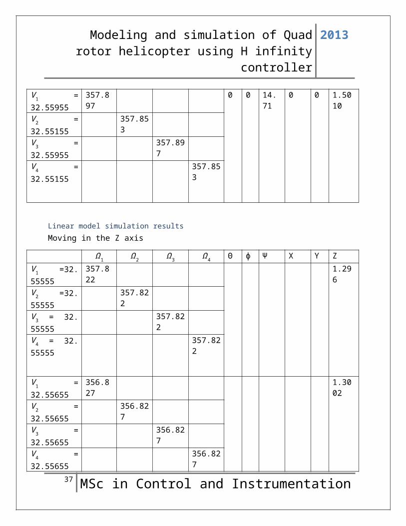
Yaw

Ω1 Ω2 Ω3 Ω4 Θ ɸ Ψ X Y ZV1 =32.55655

357.881

0 0 3.684

0 0 1.5010

V2 =32.55455

357.870

V3 = 32.55655

357.881

V4 = 32.55455

357.870

V1 =32.55755

356.886

0 0 7.359

0 0 1.5010

V2 =32.55355

356.864

V3 =32.55755

356.886

V4 =32.55355

356.864

V1 =32.55855

357.892

0 0 11.04

0 0 1.5100

V2 =32.55255

357.859

V3 =32.55855

357.892

V4 =32.55255

357.859



controller

2013

V1 =32.55955

357.897

0 0 14.71

0 0 1.5010

V2 =32.55155

357.853

V3 =32.55955

357.897

V4 =32.55155

357.853

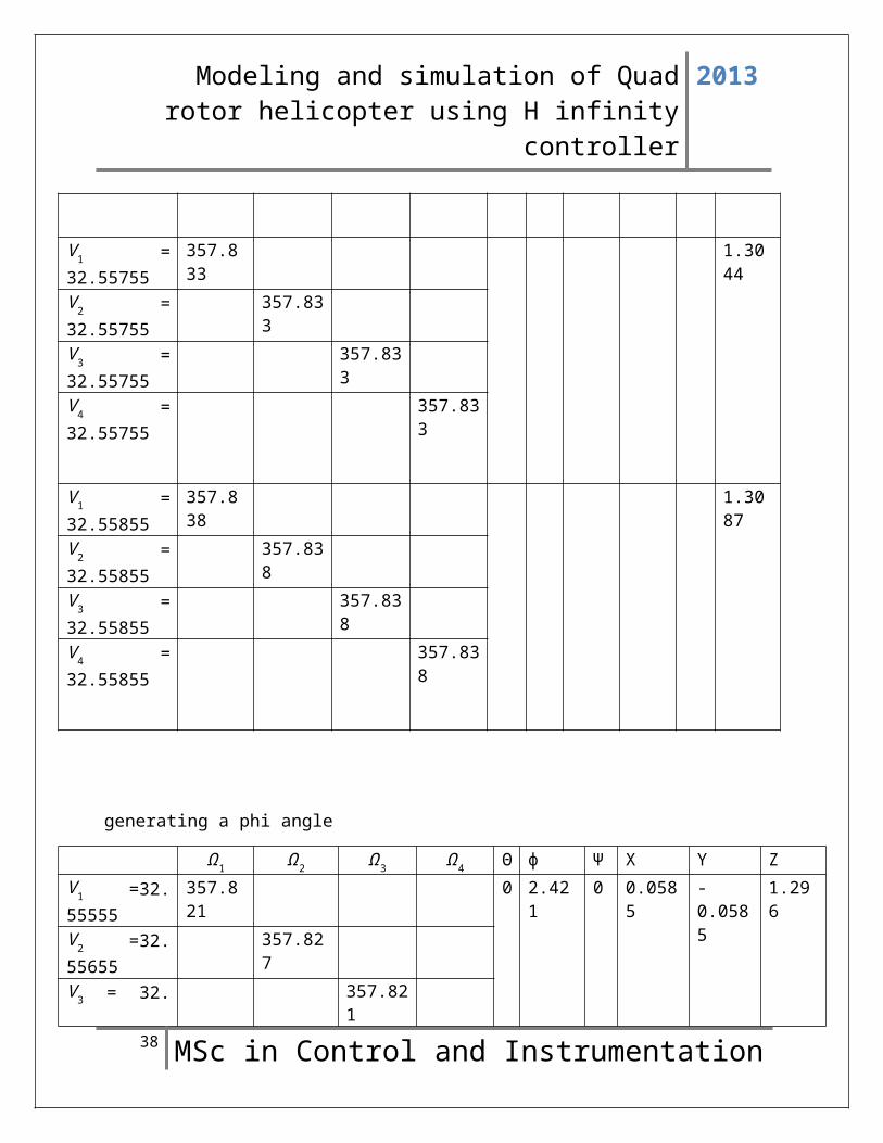
Linear model simulation resultsMoving in the Z axis

Ω1 Ω2 Ω3 Ω4 Θ ɸ Ψ X Y ZV1 =32.55555

357.822

1.296

V2 =32.55555

357.822

V3 = 32.55555

357.822

V4 = 32.55555

357.822

V1 =32.55655

356.827

1.3002

V2 =32.55655

356.827

V3 =32.55655

356.827

V4 =32.55655

356.827



controller

2013

V1 =32.55755

357.833

1.3044

V2 =32.55755

357.833

V3 =32.55755

357.833

V4 =32.55755

357.833

V1 =32.55855

357.838

1.3087

V2 =32.55855

357.838

V3 =32.55855

357.838

V4 =32.55855

357.838

generating a phi angle

Ω1 Ω2 Ω3 Ω4 Θ ɸ Ψ X Y ZV1 =32.55555

357.821

0 2.421

0 0.0585

-0.0585

1.296

V2 =32.55655

357.827

V3 = 32. 357.821



controller

2013

55555V4 = 32.55455

357.816

V1 =32.55555

356.821

0 4.841

0 0.0585

-0.0585

1.296

V2 =32.55755

356.832

V3 =32.55555

356.821

V4 =32.55355

357.810

V1 =32.55555

357.821

0 7.262

0 0.0585

-0.0585

1.296

V2 =32.55855

357.838

V3 =32.55555

357.821

V4 =32.55255

357.804

V1 =32.55555

357.821

0 9.682

0 0.0585

-0.0585

1.296

V2 =32.55955

357.844

V3 =32.55555

357.821

V4 =32.55155

357.799



controller

2013

Ω1 Ω2 Ω3 Ω4 Θ ɸ Ψ X Y ZV1 =32.55555

357.816

2.421

0 0 -0.0585

0.0585

1.296

V2 =32.55655

357.821

V3 = 32.55555

357.827

V4 = 32.55455 357.82

1V1 =32.55555

357.810

4.841

0 0 -0.0585

0.0585

1.296

V2 =32.55755

356.821

V3 =32.55555

356.832

V4 =32.55355

356.821

V1 =32.55555

357.804

7.262

0 0 -0.0585

0.0585

1.296

V2 =32.55855

357.821

V3 =32.55555

357.838

V4 =32.55255 357.82

1V1 =32.55555

357.799

9.682

0 0 -0.058

0.0585

1.296



controller

2013

5V2 =32.55955

357.821

V3 =32.55555

357.844

V4 =32.55155 357.82

1

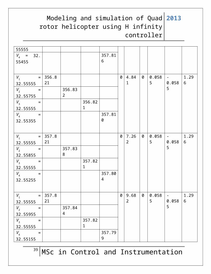
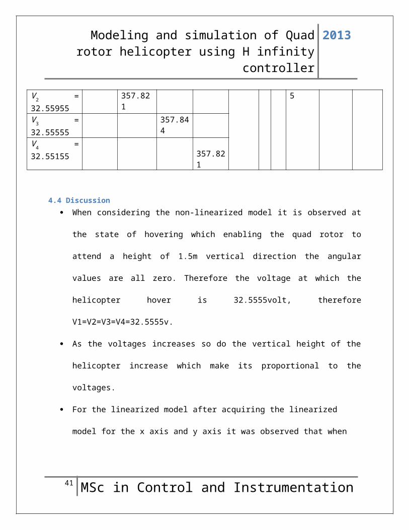
4.4 Discussion When considering the non-linearized model it is observed at

the state of hovering which enabling the quad rotor to

attend a height of 1.5m vertical direction the angular

values are all zero. Therefore the voltage at which the

helicopter hover is 32.5555volt, therefore

V1=V2=V3=V4=32.5555v.

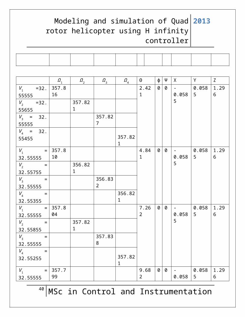
As the voltages increases so do the vertical height of the

helicopter increase which make its proportional to the

voltages.

For the linearized model after acquiring the linearized

model for the x axis and y axis it was observed that when



controller

2013

the voltage are being change that is V1 and V3 the X and Y

axis which is the distance was not moving.

Another observation noticed was that for the nonlinear model

the angular distance was affecting the movement of the

helicopter while linearize model the angular distance has no

effect on the z, y and x.

4.5 ConclusionThe objective of this test was not successful because the

linearized model for y axis and x axis is mathematically wrong so

the values when the simulation is being debugged show wrong

values.

And beside the H infinity controller was not achieved because the

group initially was supposed to use visual feedback for the model

controller but because school does not have the required

facilities or equipment (camera) for the model. So therefore the

group members decide to use another controller which is H

infinity but when the decision was made it was late for the group

to work on the controller so extra extension was ask but was42 MSc in Control and Instrumentation


controller

2013

turned down so because of the limited time the group was not able

to develop the controller for the assignment.

4.6 Reference Jianying Liu, Shiyue Liu, Qingbo Geng “ The H infinity

Control Algorithm of 3-DOF four Rotor System” Beinjin

Institute of Technology, 2012

University of Derby, Msc in control and instrumentation,

interim report, “Modelling and stimulation of Quad rotor

Helicopter’’

Tommaso Bricsciani, “Modeling, Identification and Control of

a Quad rotor helicopter”, Department of Automatic control

Lund University, October 2008.



controller

2013

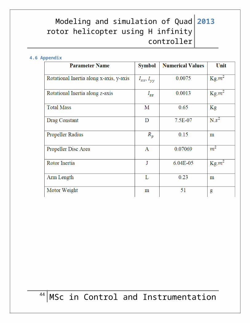
4.6 Appendix



controller

2013


quadrotor assignment

Documents