a novel overactuated quadrotor uav
TRANSCRIPT
A Novel Overactuated
Quadrotor UAV
Von der Fakultät Konstruktions-, Produktions- und Fahrzeugtechnik
der Universität Stuttgart zur Erlangung der Würde eines
Doktor-Ingenieurs (Dr.-Ing.) genehmigte Abhandlung
Vorgelegt von
Markus Ryll
aus Stuttgart
Hauptberichter: Prof. Dr.-Ing. Frank Allgöwer
Mitberichter: Prof. Dr. Heinrich H.Bülthoff
Prof. Dr. Lorenzo Marconi
Tag der mündlichen Prüfung: 06. Februar 2015
Institut für Systemtheorie und Regelungstechnik
Universität Stuttgart
2015


Acknowledgements
First of all I would like to thank my direct supervisor Dr. Paolo Robuffo Giordano for the
supervision of my thesis, his great support at any day and night time, steady encouragement
and continuous motivation. Working together with Paolo is always a great joy. I also want
to express my thankfulness to Prof. Dr. Heinrich H. Bülthoff for his support and the
promotion of my PhD by stimulating me in my research and asking critical questions in
the right moment. Prof. Dr. Heinrich H. Bülthoff created a great melting pot of scientists
from different backgrounds at the Max Planck Institute for Biological Cybernetics that is
probably unique in the world. In the same manner I want thank Prof. Dr. Frank Allgöwer,
for accepting me as his Ph.D.-student at the University of Stuttgart, without him this work
would not have been possible. Many thanks go to all the current and previous members of
the ’Autonomous Robotics and Human-Machine Systems’-group. I enjoyed every single
day spent with you in- and outside the office. As well I want to thank all the people that
accompanied me in the last 4 years and often became good friends.
I am also grateful to my family, my parents and my siblings Thomas and Karoline, for
the background they gave me. Most of all I would like to thank Katharina for always
standing by me in the office and at home. You fill my and Lotta’s life with love, happiness
and adventure.
Tübingen, July 2014
Markus Ryll
iii

Table of Contents
List of Variables ix
List of Abbreviations xiii
Abstract xv
Deutsche Kurzfassung xvii
1 Introduction 1
1.1 Summary of Contributions . . . . . . . . . . . . . . . . . . . . . . . . . . . 4
1.2 Organization of the Thesis . . . . . . . . . . . . . . . . . . . . . . . . . . . 6
2 Dynamical Model of the Holocopter 9
2.1 Preliminary definitions . . . . . . . . . . . . . . . . . . . . . . . . . . . . . 9
2.2 Equations of motion . . . . . . . . . . . . . . . . . . . . . . . . . . . . . . 11
2.3 Additional Aerodynamic Effects . . . . . . . . . . . . . . . . . . . . . . . . 13
3 Motion Control of the Holocopter 19
3.1 Control Design . . . . . . . . . . . . . . . . . . . . . . . . . . . . . . . . . 20
3.2 Optimization of Additional Criteria . . . . . . . . . . . . . . . . . . . . . . 24
3.2.1 Dynamic adaptation of wrest . . . . . . . . . . . . . . . . . . . . . . 26
3.3 Final Considerations . . . . . . . . . . . . . . . . . . . . . . . . . . . . . . 26
4 Holocopter Prototype and System Architecture 29
4.1 Prototype I . . . . . . . . . . . . . . . . . . . . . . . . . . . . . . . . . . . 29
4.1.1 Propeller motor brushless controller . . . . . . . . . . . . . . . . . . 33
4.1.2 OpenServo . . . . . . . . . . . . . . . . . . . . . . . . . . . . . . . . 34
v
Table of Contents
4.1.3 System architecture . . . . . . . . . . . . . . . . . . . . . . . . . . . 35
4.1.4 Coping with the non-idealities of the servo motors . . . . . . . . . . 38
4.2 Prototype II . . . . . . . . . . . . . . . . . . . . . . . . . . . . . . . . . . . 41
4.2.1 Mechanical design . . . . . . . . . . . . . . . . . . . . . . . . . . . . 41
4.2.2 System architecture . . . . . . . . . . . . . . . . . . . . . . . . . . . 44
4.3 Energetic efficiency of the holocopter in hovering . . . . . . . . . . . . . . . 46
5 Simulation Results 49
5.1 Ideal Simulations . . . . . . . . . . . . . . . . . . . . . . . . . . . . . . . . 50
5.1.1 Rotation on spot . . . . . . . . . . . . . . . . . . . . . . . . . . . . 50
5.1.2 Eight-shape trajectory . . . . . . . . . . . . . . . . . . . . . . . . . 51
5.1.3 Squared trajectory . . . . . . . . . . . . . . . . . . . . . . . . . . . 54
5.2 Realistic Simulations . . . . . . . . . . . . . . . . . . . . . . . . . . . . . . 57
5.2.1 Rotation on Spot . . . . . . . . . . . . . . . . . . . . . . . . . . . . 59
5.2.2 Eight-shape trajectory . . . . . . . . . . . . . . . . . . . . . . . . . 60
5.2.3 Effect of servo control frequency . . . . . . . . . . . . . . . . . . . . 63
6 Experimental Results 65
6.1 Hovering on the spot . . . . . . . . . . . . . . . . . . . . . . . . . . . . . . 65
6.2 Rotation on Spot . . . . . . . . . . . . . . . . . . . . . . . . . . . . . . . . 67
6.3 Eight-shape trajectory . . . . . . . . . . . . . . . . . . . . . . . . . . . . . 68
6.4 Combined trajectory . . . . . . . . . . . . . . . . . . . . . . . . . . . . . . 68
6.5 Summary . . . . . . . . . . . . . . . . . . . . . . . . . . . . . . . . . . . . 72
7 Perspectives on Aerial Interaction 75
7.1 Admittance control . . . . . . . . . . . . . . . . . . . . . . . . . . . . . . . 76
7.2 Force Observer . . . . . . . . . . . . . . . . . . . . . . . . . . . . . . . . . 79
7.3 Outline . . . . . . . . . . . . . . . . . . . . . . . . . . . . . . . . . . . . . . 80
8 Conclusions 83
vi

Table of Contents
Appendix 85
A Technical Proofs 87
B Schematics 91
B.1 Mechanical schematics . . . . . . . . . . . . . . . . . . . . . . . . . . . . . 91
B.2 Electrical schematics . . . . . . . . . . . . . . . . . . . . . . . . . . . . . . 103
Bibliography 109
vii

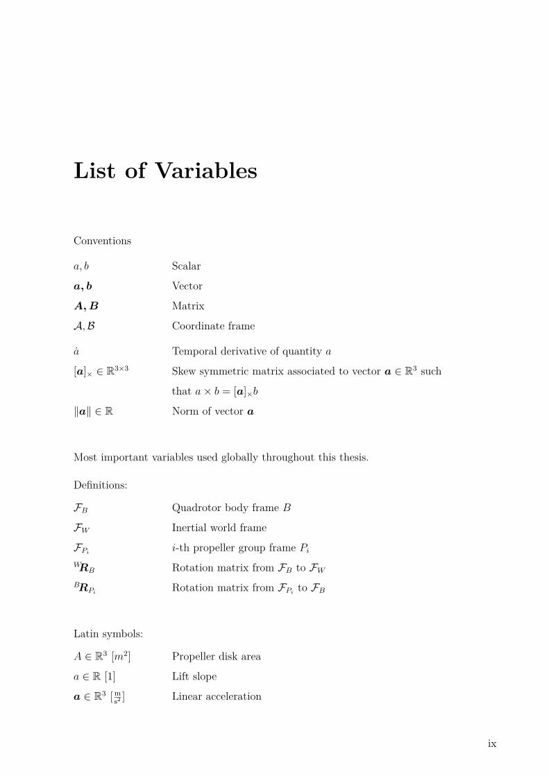
List of Variables
Conventions
a, b Scalar
a, b Vector
A,B Matrix
A,B Coordinate frame
a Temporal derivative of quantity a
[a]× ∈ R3×3 Skew symmetric matrix associated to vector a ∈ R3 such
that a× b = [a]×b
‖a‖ ∈ R Norm of vector a
Most important variables used globally throughout this thesis.
Definitions:
FB Quadrotor body frame B
FW Inertial world frame
FPii-th propeller group frame Pi
WRB Rotation matrix from FB to FWBRPi
Rotation matrix from FPito FB
Latin symbols:
A ∈ R3 [m2] Propeller disk area
a ∈ R [1] Lift slope
a ∈ R3 [ms2 ] Linear acceleration
ix
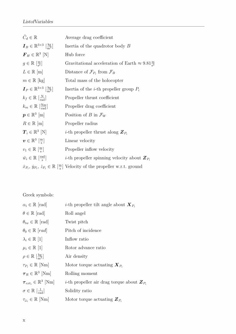
ListofVariables
Cd ∈ R Average drag coefficient
IB ∈ R3×3 [ kgm2 ] Inertia of the quadrotor body B
FH ∈ R3 [N] Hub force
g ∈ R [ms2 ] Gravitational acceleration of Earth ≈ 9.81ms2
L ∈ R [m] Distance of FPifrom FB
m ∈ R [kg] Total mass of the holocopter
IP ∈ R3×3 [ kgm2 ] Inertia of the i-th propeller group Pikf ∈ R [ N
rad ] Propeller thrust coefficient
km ∈ R [Nmrad ] Propeller drag coefficient
p ∈ R3 [m] Position of B in FWR ∈ R [m] Propeller radius
T i ∈ R3 [N] i-th propeller thrust along ZPi
v ∈ R3 [ms ] Linear velocity
v1 ∈ R [ms ] Propeller inflow velocity
wi ∈ R [ rads ] i-th propeller spinning velocity about ZPi
xPi, yPi
, zPi∈ R [ms ] Velocity of the propeller w.r.t. ground
Greek symbols:
αi ∈ R [rad] i-th propeller tilt angle about XPi
θ ∈ R [rad] Roll angel
θtw ∈ R [rad] Twist pitch
θ0 ∈ R [rad] Pitch of incidence
λi ∈ R [1] Inflow ratio
µi ∈ R [1] Rotor advance ratio
ρ ∈ R [ kgm3 ] Air density
τPi∈ R [Nm] Motor torque actuating XPi
τR ∈ R3 [Nm] Rolling moment
τ exti ∈ R3 [Nm] i-th propeller air drag torque about ZPi
σ ∈ R [ 1rad ] Solidity ratio
τωi∈ R [Nm] Motor torque actuating ZPi
x
List of Variables
φ ∈ R [rad] Pitch angel
ψ ∈ R3 [rad] Yaw angel
ωB ∈ R3 [ rads ] Angular velocity of B in FB
All other symbols are only defined locally for one section and might be used in other sections
in a different context. This allowed the authors to adapt to common notations and symbols
whenever possible. For the reader’s convenience most important symbols of a section are
summarized in tables in the same section.
xi

List of Abbreviations
A/D Analog/Digital
ATX Advanced Technology eXtended
BL-Ctrl Brushless controller
CAD Computer-aided design
CAN Controller area network
DC Direct current
DDR2 Double Data Rate 2
dof Degree of freedom
e.g. Exempli gratia
EC Electronically commutated
Fig. Figure
I2C Inter-Integrated Circuit
i.e Id est
IMU Inertial measurement unit
LTS Long-term support
MAV Micro aerial vehicel
MEMS Microelectromechanical systems
MoCap Motion capture system
MOSFETS Metal-oxide-semiconductor field-effect transistor
OS Operating system
PC Personal computer
PID Proportional-integral-derivative
PWM Pulse-width modulation
RAM Random-access memory
xiii
ListofAbbreviations
RC Remote control
Sect. Section
TTL Transistor-transistor logic
UAV Unmanned aerial vehicle
USB Universal Serial Bus
w.r.t. With respect to
xiv
Abstract
Standard quadrotor UAVs are inherently underactuated as they posses only four independent
control inputs - their four propeller spinning velocities. Therefore they only possess a
limited mobility in space for the six dofs parameterizing the quadrotor position/orientation.
This implies that for standard quadrotors it is impossible to follow an arbitrarily designed
trajectory. A standard quadrotor for example cannot translate position while remaining
horizontal. The common use of UAVs and quadrotors in particular is changing from
common observer tasks to more applied flying service robot tasks including interaction with
the environment. Here the loss of mobility on the basis of the inherent underactuation
can constitute a limiting factor. In this thesis we will present a novel quadrotor UAV
design that surmounts these limitations by additional four control inputs actuating the
four propeller tilting angles. First, we will show that our novel quadrotor UAV with
tilting propellers offers behavior as a fully-actuated flying vehicle with full actuation of
the quadrotor position and orientation in space. Second, a comprehensive modeling and
control framework for the proposed quadrotor is presented, and the hardware/software
specifications of an experimental prototype will be introduced. Finally, the results of several
simulations and real experiments are reported to illustrate the capabilities of the proposed
novel UAV design.
xv


Deutsche Kurzfassung
Neue Ansätze zur Regelung über-
aktuierter, unbemannte Luftfahr-
zeuge
Unbemannte Quadrocopter und ähnliche Luftfahrzeuge (z.B. Hubschrauber) haben eine
eingeschränkte Manövrierbarkeit aufgrund ihres konzeptuell unteraktuierten Systems. Das
heißt diese Luftfahrzeuge besitzen weniger Steuereingänge (im Falle von Quadrocoptern die
vier Rotationsgeschwindigkeiten der Rotoren) als die sechs translatorischen und rotatori-
schen Freiheitsgrade eines Körpers im Raum. Daraus folgt das diese Luftfahrzeuge einer
beliebigen Trajektorie im Raum nicht notwendigerweise folgen können. Beispielsweiße ist
eine horizontale Translation ohne Rotation nicht möglich. Da unbemannte Luftfahrzeuge
mehr und mehr als fliegende Serviceroboter, die auf ihre Umgebung einwirken, verwendet
werden, ist dieser Mangel an Mobilität ein grundsätzlich limitierender Faktor. In dieser
Doktorarbeit wird ein konstruktiv neuartiger Entwurf eines Luftfahrzeuges vorgestellt -
der Holocopter. Beim Holocopter ist zusätzlich die Orientierung der Rotoren regelbar,
hier durch ist die beschriebene Unteraktuierung nicht mehr gegeben. Das System ist nun
überaktuiert, da den nun acht Steuereingängen sechs Freiheitsgrade gegenüberstehen. Die
vier zusätzlichen Steuereingänge ermöglichen eine vollständige Steuerbarkeit der Position
und Orientierung des Holocopters im Raum. Daher lässt sich der Holocopter als vollständig
steuerbarer, fliegender Roboter verwenden. In dieser Arbeit wurde zunächst ausführlich
das kinematische Modell des Holocopters hergeleitet und ein passender Regler basierend
auf dynamischer, linearisierter Zustandsrückführung entworfen. Anschließend wurde ein
xvii

Deutsche Kurzfassung
Prototyp entworfen und gebaut und das nötige Software-Framework entwickelt. Zentraler
Bestandteil der Arbeit sind ausführliche Simulationen und tatsächliche Tests mit den
Prototypen. Abschließend bietet die Arbeit einen Ausblick auf Interaktionsszenarios des
Holocopters mit der Umgebung.
xviii
Chapter 1
Introduction
In the past decade research on Unmanned Aerial Vehicles (UAVs) experienced an enormous
increment of growth (see e.g. Bouabdallah et al. (2007); Gurdan et al. (2007); Mellinger et al.
(2010); Pounds et al. (2010); Valavanis (2007)). A literature research lists 117 publications
containing the phrase "‘Unmanned Aerial Vehicles"’ in major journals and conferences in
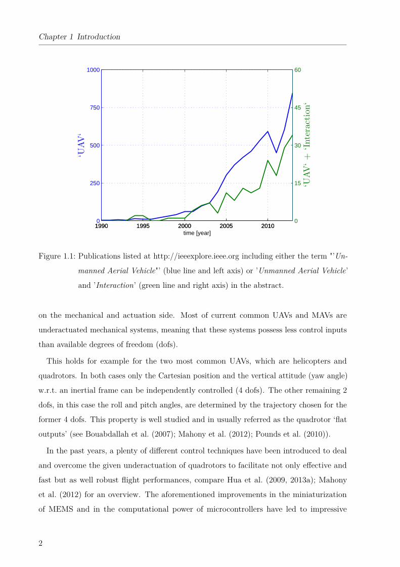
2003. In 2008 this are already 459 publications while in 2013 it exceeds 845 articles (see
figure 1.1). In particular micro aerial vehicles (MAVs) contribute to this interest. This
vast growth is due to several facts e.g. advances in microelectromechanical systems and
sensors (MEMS), increasing computational power of microcontrollers and miniaturized
computer systems, improvements in energy storage on batteries and the overall decreasing
costs for UAVs. All this offers new application areas for UAVs and MAVs in various fields
like search and rescue missions, data collection, autonomous exploration and surveillance
in inaccessible disaster areas, beneficial from a research point of view as well as for our
society. While MAV research in its beginning mainly focused on general control of the MAV
system and it localization (here self localization and mapping has to be mentioned) a new
topic rose in the last years - the transitional use of MAVs from ‘autonomous flying vehicles’
into more robotic oriented ‘autonomous flying service robots’. This means a transition
from pure observer tasks to the possibility of actual interaction with the environment
either by robust incidental interaction (Briod (2014)), simple grasping/manipulation tasks
(Lindsey et al. (2011); Pound et al. (2011)) or desired long term contact in the meaning of
manipulation (Gentili et al. (2008); Gioioso et al. (2014); Naldi and Marconi (2010)). The
extension of tasks as well as their complexity demands as well innovative breakthroughs
1
Chapter 1 Introduction
1990 1995 2000 2005 20100
250
500
750
1000
‘UAV‘
1990 1995 2000 2005 20100
15
30
45
60
‘UAV‘+
‘Interaction‘
time [year]
Figure 1.1: Publications listed at http://ieeexplore.ieee.org including either the term "’Un-
manned Aerial Vehicle"’ (blue line and left axis) or ’Unmanned Aerial Vehicle’
and ’Interaction’ (green line and right axis) in the abstract.
on the mechanical and actuation side. Most of current common UAVs and MAVs are
underactuated mechanical systems, meaning that these systems possess less control inputs
than available degrees of freedom (dofs).
This holds for example for the two most common UAVs, which are helicopters and
quadrotors. In both cases only the Cartesian position and the vertical attitude (yaw angle)
w.r.t. an inertial frame can be independently controlled (4 dofs). The other remaining 2
dofs, in this case the roll and pitch angles, are determined by the trajectory chosen for the
former 4 dofs. This property is well studied and in usually referred as the quadrotor ‘flat
outputs’ (see Bouabdallah et al. (2007); Mahony et al. (2012); Pounds et al. (2010)).
In the past years, a plenty of different control techniques have been introduced to deal
and overcome the given underactuation of quadrotors to facilitate not only effective and
fast but as well robust flight performances, compare Hua et al. (2009, 2013a); Mahony
et al. (2012) for an overview. The aforementioned improvements in the miniaturization
of MEMS and in the computational power of microcontrollers have led to impressive
2
achievements by employing quadrotor UAVs as robotics platforms: planning and control
for aggressive flight maneuvers (Mellinger et al. (2010)), collective control of multiple small-
and micro-quadrotors (Franchi et al. (2012); Kushleyev et al. (2012)), and vision-based
state estimation for autonomous flight (Shen et al. (2013)) are just a few examples.
However the underactuated design of most common UAVs still limits on one hand the
maneuverability in either free or cluttered environments and on the other hand and probably
even more importantly corrupts diversity of possible interactions with the environment by
exerting desired but arbitrary forces and torques in all directions. In particular this limiting
factor determines common quadrotor UAVs while they are more and more exploited as
autonomous flying service robots. Flying robots is a vast growing academic and economic
branch of robotics as e.g. proven by the recently funded EU projects “AIRobots” EU
Collaborative Project ICT-248669 AIRobots and “ARCAS” EU Collaborative Project
ICT-287617 ARCAS. Indeed, several groups have been addressing the possibility to allow
for an actual interaction with the environment, either in the form of direct contact Gentili
et al. (2008); Marconi and Naldi (2012); Naldi and Marconi (2010) or by considering aerial
grasping/manipulation tasks Lindsey et al. (2011); Manubens et al. (2013); Pound et al.
(2011); Spica et al. (2012); Sreenath and Kumar (2013). In this respect, as also recognized
in Hua et al. (2013b); Long and Cappelleri (2013), it is interesting to explore different
actuation strategies that can overcome the aforementioned underactuation problem and
allow for full motion and force control in all directions in space.
Motivated by these considerations, several solutions have been proposed in the past liter-
ature spanning different concepts as, e.g., using multiple UAVs to manipulate a cable-towed
object Manubens et al. (2013), ducted-fan designs Naldi et al. (2010), tilt-wing mecha-
nisms Oner et al. (2008, 2009), UAVs with non-parallel (but fixed) thrust directions Voyles
and Jiang (2012), or tilt-rotor actuations Kendoul et al. (2006); Sanchez et al. (2008).
In Forte et al. (2012b), the possibility of combining several modules of underactuated
ducted-fan vehicles to achieve full 6-dof actuation for the assembled robot is theoretically
explored, with a special focus on the optimal allocation of the available (redundant) control
inputs. In contrast, the authors of Hua et al. (2013b) consider the possibility of a ‘thrust-
tilted’ quadrotor UAV in which the main thrust direction (2 dofs) can be actively regulated.
A trajectory tracking control strategy is then proposed, which is able to explicitly take
3
Chapter 1 Introduction
into account a limited range of the thrust tilting angles. Finally, in Long and Cappelleri
(2013) a UAV made of two central coaxial counter-rotating propellers surrounded by three
tilting thrusters has been presented along with some preliminary experimental results. The
prototype is capable of two flight modalities: a ‘fixed configuration’ in which it essentially
behaves as a standard underactuated UAV, and a ‘variable angle’ configuration which
guarantees some degree of full actuation as shown in the reported results.
1.1 Summary of Contributions
Inspired by the aforementioned works for this theses we opted for a novel actuation concept
of a quadrotor UAV with propellers actuated revolvable about the axes connecting them to
the main body frame Falconi and Melchiorri (2012); Ryll et al. (2012, 2013). As explained
before standard quadrotor designs suffer from their intrinsic underactuation with only 4
control inputs (spinning velocity of the 4 rotors) which prevents an independent control
of the position and orientation of the UAV at the same time. For example, for classical
quadrotors lateral transitions are impossible without changing the attitude to accelerate into
the desired lateral direction. In other words classical quadrotors can hover only stationary
if the plane in which the motors lie is parallel to the ground plane (vertical to gravity
vector). In opposition to standard quadrotors the presented quadrotor is able to gain full
controllability over position and orientation by exploiting the additional actuation of the
propeller orientation, thus transforming it, as a matter of fact, in a fully actuated flying
rigid body1. Apart from the challenges inherent to the control design for this novel UAV,
we believe that endowing UAVs with full 6 dofs mobility will represent an important feature
in many future applications, especially those involving interaction and manipulation as well
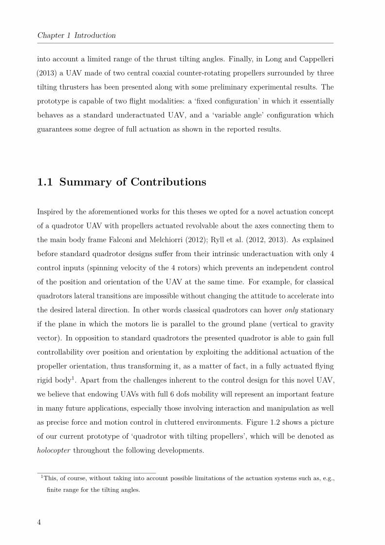
as precise force and motion control in cluttered environments. Figure 1.2 shows a picture
of our current prototype of ‘quadrotor with tilting propellers’, which will be denoted as
holocopter throughout the following developments.
1This, of course, without taking into account possible limitations of the actuation systems such as, e.g.,
finite range for the tilting angles.
4
1.1 Summary of Contributions
Figure 1.2: Picture of the holocopter prototype. The four propeller groups are slightly
tilted. The red bar indicates the positive direction of the XB holocopter body
axis
5
Chapter 1 Introduction
1.2 Organization of the Thesis
The thesis, as well as its main contributions, are organized as follows:
1. a complete dynamical model of the holocopter is first derived in Sect. 2 by taking
into account the dominant aerodynamic forces/torques (the propeller actuation), and
by analyzing the effects of the main neglected terms;
2. a trajectory tracking controller is then presented in Sect. 3 aimed at exploiting the
actuation capabilities of the holocopter for tracking arbitrary trajectories for its body
position and orientation. As the holocopter is actually overactuated (8 control inputs
for 6 controlled dofs), suitable strategies to exploit the actuation redundancy are also
discussed: these are aimed at preserving full controllability of the holocopter pose
and at minimizing the total energy consumption during flight;
3. a thorough description of the hardware/software architecture of the prototype shown
in Fig. 1.2 is then given in Sect. 4, including the identification of its dynamical
parameters and a discussion of the main non-idealities w.r.t. the dynamical model
developed in Sect. 2. In particular, a predictive scheme complementing the control
action of Sect. 3 is introduced in order to cope with the poor performance of the
employed servo motors. Subsequently the hardware/software architecture of the
improved and more advanced second prototype that is currently under final testing is
as well thoroughly discussed and described;
4. an extensive set of ideal/realistic simulations and experimental results on the holo-
copter prototype is then presented in Sects. 5–8, showing the appropriateness of the
various modeling assumptions and of the adopted control design. A video collecting
several experimental flights is also available at http://youtu.be/hA-uNHW8MLE;
5. an outline of future developments on the control design for enabling interaction tasks
is presented focusing on an admittance based control scheme utilizing the position
controller presented in Sect. 3 and an force/torque observer to avoid the need of a
force/torque sensor;
6. conclusions and some future discussions are then given in Sect. 8 with a focus on
interaction tasks and the second prototype;
6
1.2 Organization of the Thesis
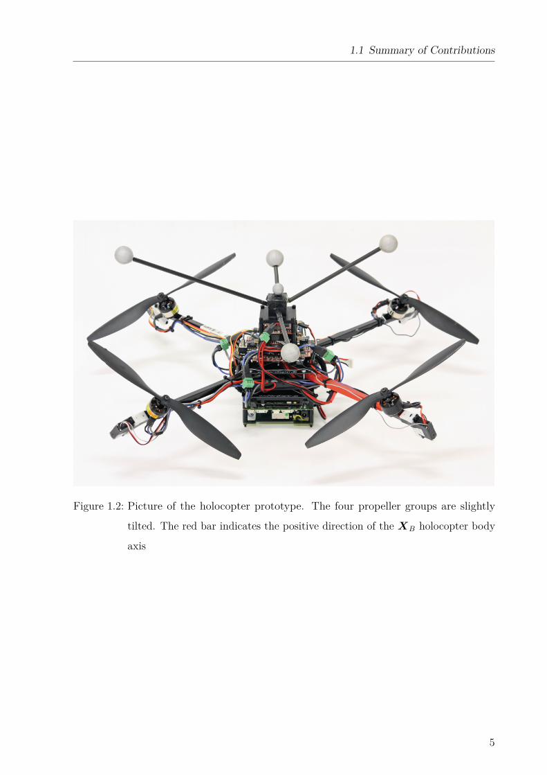
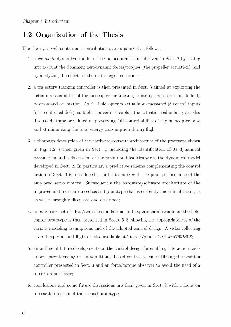
Figure 1.3: CAD model of the quadrotor with tilting propellers. The model is based on a
quadrotor from mikrokopter.de, and is composed of: (1) Micro controller, (2)
Brushless controller, (3) Lander, (4) Propeller motor, (5) Tilting actuator, (6)
Battery.
We finally note that parts of this thesis have already been published in Ryll et al. (2012,
2013, to be published 2014).
7

Chapter 2
Dynamical Model of the Holocopter
This chapter has been mainly reproduced from an article published in ICRA 2012: Ryll
et al. (2012)
The quadrotor analyzed in this thesis can be considered as a connection of 5 main
rigid bodies in relative motion among themselves: the quadrotor body itself B and the
4 propeller groups Pi. These consist of the propeller arm hosting the motor responsible
for the tilting actuation mechanism, and the propeller itself connected to the rotor of the
motor responsible for the propeller spinning actuation1 (see Figs. 1.2–2.2). The aim of this
Section is to derive the equations of motion of this multi-body system.
2.1 Preliminary definitions
Let FW : {OW ; XW , Y W , ZW} be a world inertial frame and FB : {OB; XB, Y B, ZB}
a moving frame attached to the quadrotor body at its center of mass (see Fig. 2.1). We
also define FPi: {OPi
; XPi, Y Pi
, ZPi}, i = 1 . . . 4, as the frames associated to the i-th
propeller group, with XPirepresenting the tilting actuation axis and ZPi
the propeller
actuated spinning (thrust Ti) axis (see Fig. 2.2).
As usual, we let 1R2 ∈ SO(3) be the rotation matrix representing the orientation of frame
2 w.r.t. frame 1: therefore, WRB will represent the orientation of the body frame w.r.t. the
world frame, while BRPithe orientation of the propeller group i-th frame w.r.t. the body
1For simplicity we are here considering each propeller groups Pi as a ‘single body approximation’ of both
the propeller/rotor and its hoisting mechanism.
9
Chapter 2 Dynamical Model of the Holocopter
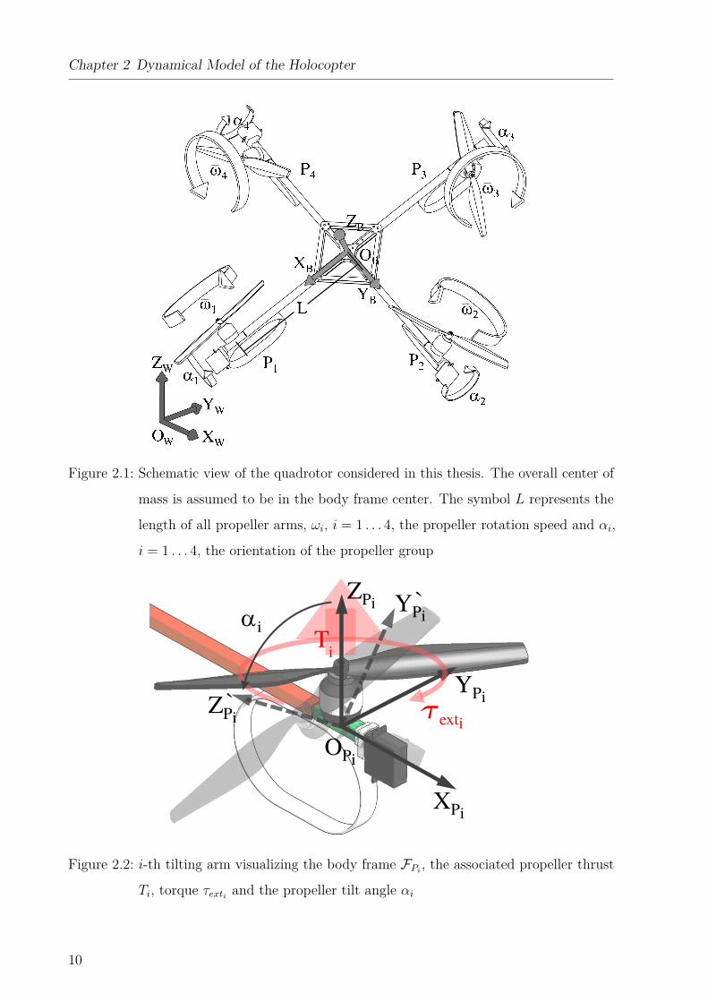
Figure 2.1: Schematic view of the quadrotor considered in this thesis. The overall center of
mass is assumed to be in the body frame center. The symbol L represents the
length of all propeller arms, ωi, i = 1 . . . 4, the propeller rotation speed and αi,
i = 1 . . . 4, the orientation of the propeller group
XPi
YPi
ZPi
ZPi
YPi
`
` αi
OPi
Ti
texti
Figure 2.2: i-th tilting arm visualizing the body frame FPi, the associated propeller thrust
Ti, torque τexti and the propeller tilt angle αi
10
2.2 Equations of motion
frame. By denoting with αi ∈ R the propeller tilt angle about axis XPi, it follows from
Fig. 2.1 that2
BRPi= RZ
((i− 1)π2
)RX(αi), i = 1 . . . 4.
Similarly, we also let
BOPi= RZ
((i− 1)π2
)L
0
0
, i = 1 . . . 4
be the origin of the propeller frames FPiin the body frame with L being the distance of
OPifrom OB.
Summarizing, the quadrotor configuration is completely determined by the body position
p = WOB ∈ R3 and orientation WRB in the world frame, and by the 4 tilt angles αispecifying the propeller group orientations in the body frame (rotations about XPi
). We
omit the propeller spinning angles about ZPias configuration variables, although the
propeller spinning velocities wi about ZPiwill be part of the system model (see next
Sections).
2.2 Equations of motion
By exploiting standard techniques (e.g., Newton-Euler procedure), it is possible to derive a
complete description of the quadrotor dynamic model by considering the forces/moments
generated by the propeller motion, as well as any cross-coupling due to gyroscopic and
inertial effects arising from the relative motion of the 5 bodies composing the quadrotor. As
aerodynamic forces and torques, we will only consider those responsible for the quadrotor
actuation and neglect any additional second-order effects/disturbances. Indeed, as discussed
in the next Sect. 2.3, for the typical ‘slow’ flight regimes considered in this work, the propeller
actuation forces and torques result significantly dominant w.r.t. other aerodynamic effects.
We now discuss in detail the main conceptual steps needed to derive the quadrotor dynamical
model.2Throughout the following, RX(θ), RY (θ), RZ(θ) will denote the canonical rotation matrixes about the
X, Y , Z axes of angle θ, respectively.
11
Chapter 2 Dynamical Model of the Holocopter
To this end, let ωB ∈ R3 be the angular velocity of the quadrotor body B expressed in
the body frame3, and consider the i-th propeller group Pi. The angular velocity of the i-th
propeller (i.e., of FPi) w.r.t. FW and expressed in FPi
is just
ωPi= BRT
PiωB + [αi 0 wi]T ,
where αi is the tilting velocity about XPiand wi ∈ R the spinning velocity about ZPi
,
both w.r.t. FB (see Sect. 2.1). This results in an angular acceleration
ωPi= BRT
PiωB + BR
T
PiωB + [αi 0 ˙wi]T .
By applying the Euler equations of motion, it follows that
τ Pi= IPi
ωPi+ ωPi
× IPiωPi− τ exti . (2.1)
Here, IPi∈ R3×3 is the (constant) symmetric and positive definite inertia matrix of the
i-th propeller/rotor assembly approximated as an equivalent disc (the inertia of the tilting
mechanism is supposed lumped into the main body B), and τ exti any external torque
applied to the propeller. As usual, see e.g. Valavanis (2007), we assume presence of a
counter-rotating torque about the ZPiaxis caused by air drag and modeled as
τ exti = [0 0 − kmωPiZ|ωPiZ
|]T , km > 0 (2.2)
with ωPiZbeing the third component of ωPi
.
Let now
T Pi= [0 0 kf wi|wi|]T , kf > 0, (2.3)
represent the i-th propeller force (thrust) along the ZPiaxis and acting at BOPi
in FB. By
considering the quadrotor body B and the torques generated by the four propellers Pi, one
then obtains4∑i=1
(BOPi
×BRPiT Pi− BRPi
τ Pi
)= IBωB + ωB × IBωB, (2.4)
with IB ∈ R3×3 being the (constant) symmetric and positive definite Inertia matrix of B.
As for the translational dynamics, we assume for simplicity that the barycenter of each
propeller group Pi coincides with OPi. This allows us to neglect inertial effects on the
3In the following, we will assume that every quantity is expressed in its own frame, e.g., ωB =BωB .
12
2.3 Additional Aerodynamic Effects
propeller groups due to the quadrotor body acceleration in space. Therefore, by recalling
that p = WOB is the quadrotor body position in world frame, one has
mp = m
0
0
−g
+ WRB
4∑i=1
BRPiT Pi
(2.5)
wherem is the total mass of the quadrotor and propeller bodies and g the scalar gravitational
acceleration of Earth.
Summarizing, equations (2.1)–(2.4)–(2.5) describe the rotational/translational dynamics
of the quadrotor body and propeller groups. Note that the inputs of this model are the motor
torques actuating the propeller tilting axes XPiand spinning axes ZPi
. These are denoted
as ταi= τ TPi
XPi∈ R and τwi
= τ TPiZPi∈ R, i = 1 . . . 4, respectively, for a total of 4 + 4 = 8
independent control torques (inputs). The propeller spinning velocities wi (actuated by τwi)
will then generate the forces and torques affecting the translational/rotational motion of
the quadrotor body B as a function of its current configuration, in particular of the tilting
angles αi actuated by ταi. For the reader’s convenience, Table 2.1 lists the main quantities
introduced in this section.
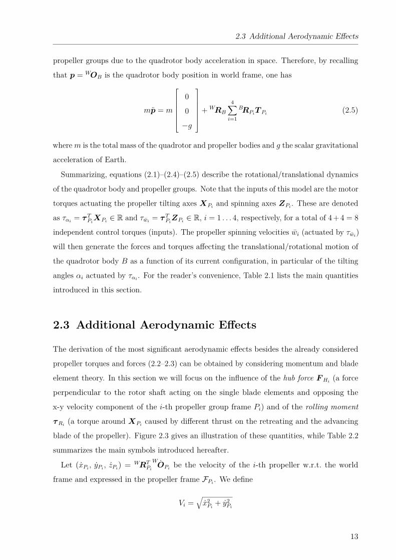
2.3 Additional Aerodynamic Effects
The derivation of the most significant aerodynamic effects besides the already considered
propeller torques and forces (2.2–2.3) can be obtained by considering momentum and blade
element theory. In this section we will focus on the influence of the hub force FHi(a force
perpendicular to the rotor shaft acting on the single blade elements and opposing the
x-y velocity component of the i-th propeller group frame Pi) and of the rolling moment
τRi(a torque around XPi
caused by different thrust on the retreating and the advancing
blade of the propeller). Figure 2.3 gives an illustration of these quantities, while Table 2.2
summarizes the main symbols introduced hereafter.
Let (xPi, yPi
, zPi) = WRT
Pi
WOPi
be the velocity of the i-th propeller w.r.t. the world
frame and expressed in the propeller frame FPi. We define
Vi =√x2Pi
+ y2Pi
13
Chapter 2 Dynamical Model of the Holocopter
Symbols Definitions
FW inertial world frame
FB quadrotor body frame B
FPii-th propeller group frame Pi
p position of B in FWWRB rotation matrix from FB to FWBRPi
rotation matrix from FPito FB
αi i-th propeller tilt angle about XPi
wi i-th propeller spinning velocity about ZPi
ωB angular velocity of B in FBτ exti i-th propeller air drag torque about ZPi
T i i-th propeller thrust along ZPi
τPimotor torque actuating XPi
τωimotor torque actuating ZPi
m total mass of the holocopter
IP inertia of the i-th propeller group PiIB inertia of the quadrotor body B
kf propeller thrust coefficient
km propeller drag coefficient
L distance of FPifrom FB
g gravitational acceleration of Earth
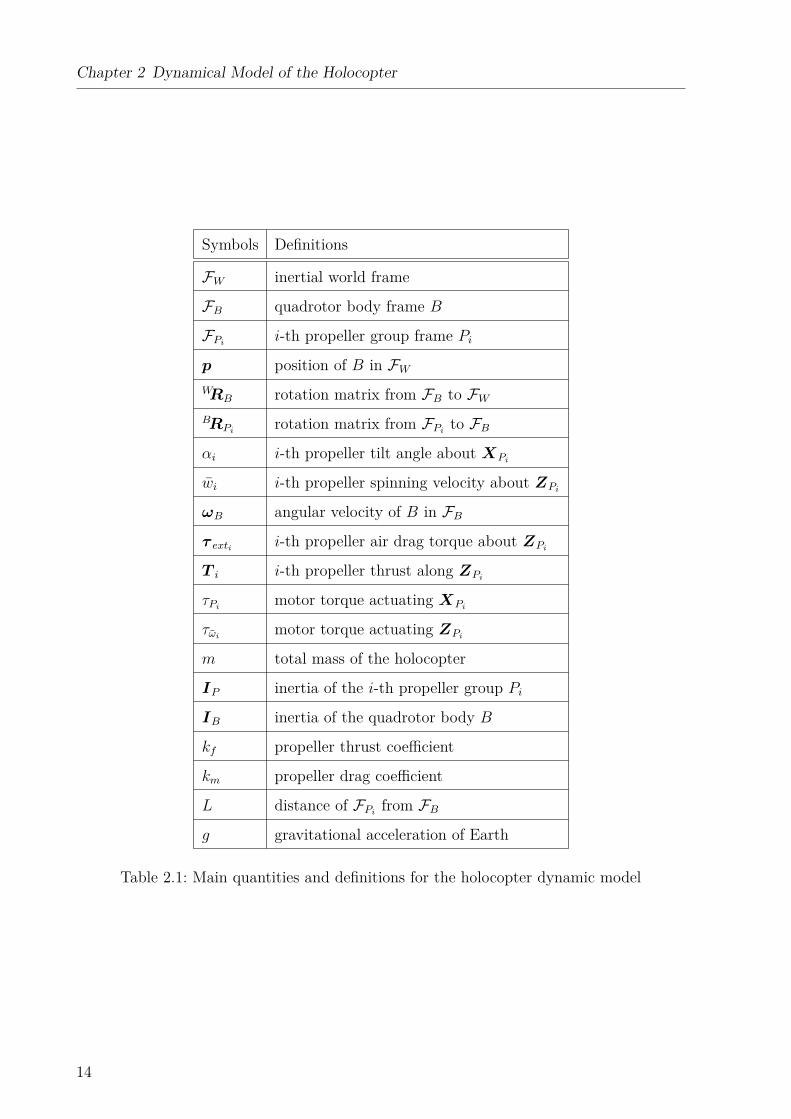
Table 2.1: Main quantities and definitions for the holocopter dynamic model
14
2.3 Additional Aerodynamic Effects
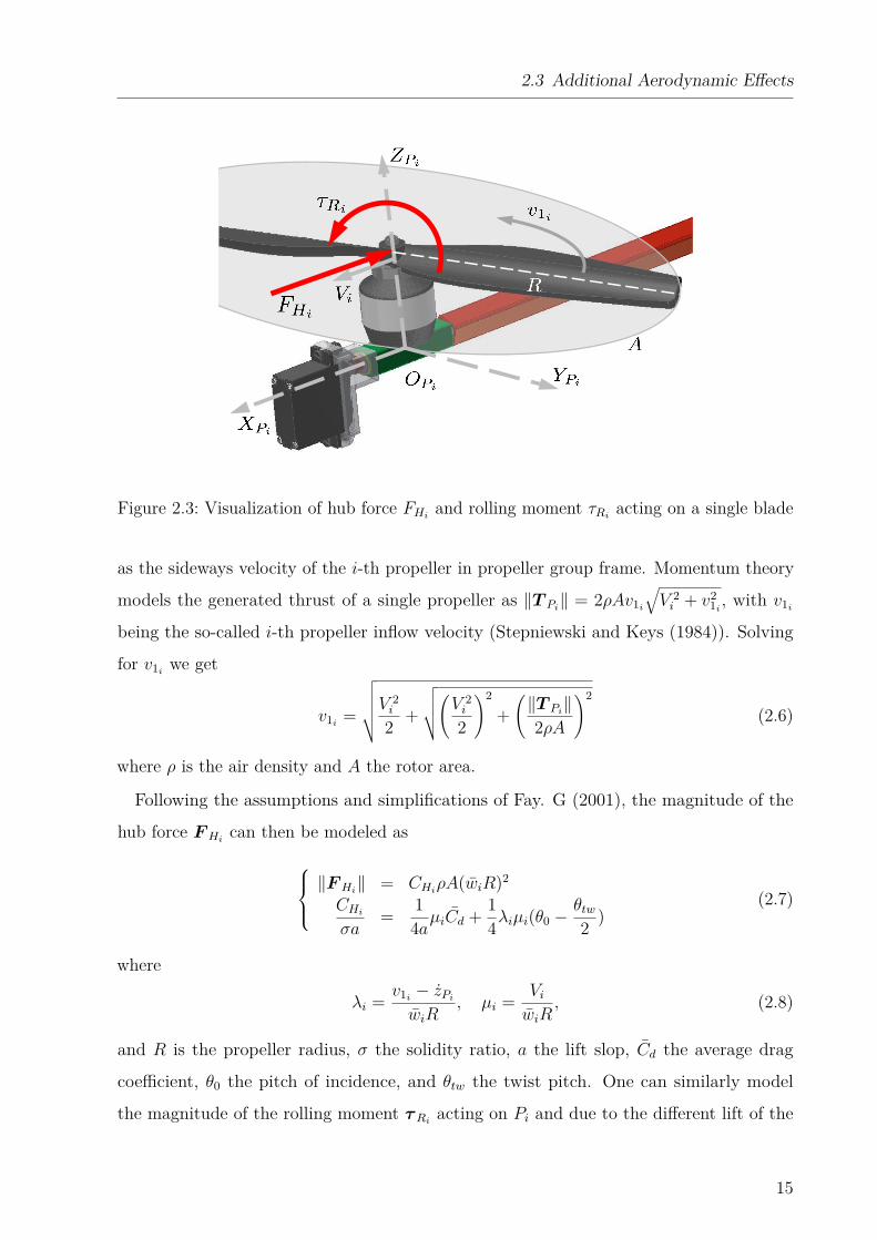
Figure 2.3: Visualization of hub force FHiand rolling moment τRi
acting on a single blade
as the sideways velocity of the i-th propeller in propeller group frame. Momentum theory
models the generated thrust of a single propeller as ‖T Pi‖ = 2ρAv1i
√V 2i + v2
1i, with v1i
being the so-called i-th propeller inflow velocity (Stepniewski and Keys (1984)). Solving
for v1iwe get
v1i=
√√√√√V 2i
2 +
√√√√(V 2i
2
)2
+(‖T Pi
‖2ρA
)2
(2.6)
where ρ is the air density and A the rotor area.
Following the assumptions and simplifications of Fay. G (2001), the magnitude of the
hub force FHican then be modeled as
‖FHi
‖ = CHiρA(wiR)2
CHi
σa= 1
4aµiCd + 14λiµi(θ0 −
θtw2 )
(2.7)
where
λi = v1i− zPi
wiR, µi = Vi
wiR, (2.8)
and R is the propeller radius, σ the solidity ratio, a the lift slop, Cd the average drag
coefficient, θ0 the pitch of incidence, and θtw the twist pitch. One can similarly model
the magnitude of the rolling moment τRiacting on Pi and due to the different lift of the
15
Chapter 2 Dynamical Model of the Holocopter
0 5 10 15 20 25 30 35 40 450
1
2
3
4
5
6
7
8
||T1||[N
]
time [s]0 5 10 15 20 25 30 35 40 45
0
0.01
0.02
0.03
0.04
||FH
1||[N
](a)
0 5 10 15 20 25 30 35 40 450
0.02
0.04
0.06
0.08
0.1
0.12
0.14
0.16
||τext 1||[N
m]
time [s]0 5 10 15 20 25 30 35 40 45
0
0.01
0.02
0.03
0.04
||τR
1||[N
m]
(b)
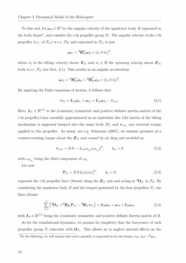
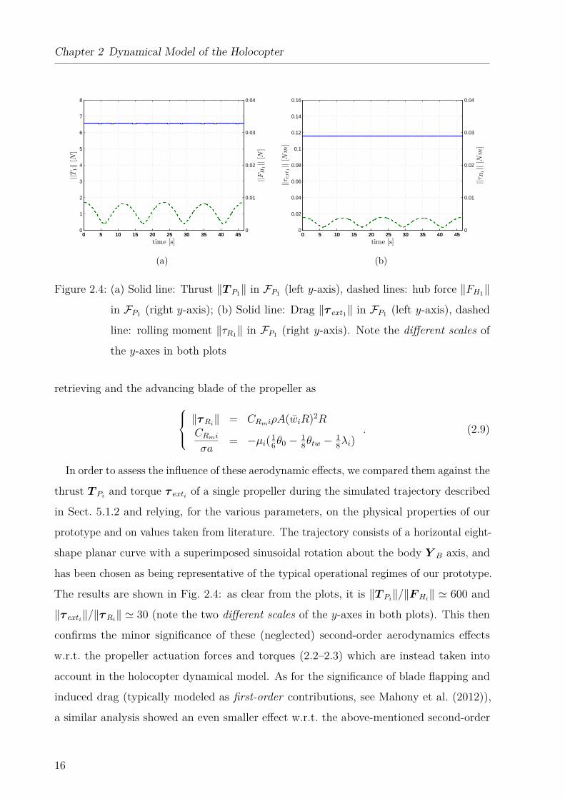
Figure 2.4: (a) Solid line: Thrust ‖T P1‖ in FP1 (left y-axis), dashed lines: hub force ‖FH1‖
in FP1 (right y-axis); (b) Solid line: Drag ‖τ ext1‖ in FP1 (left y-axis), dashed
line: rolling moment ‖τR1‖ in FP1 (right y-axis). Note the different scales of
the y-axes in both plots
retrieving and the advancing blade of the propeller as‖τRi‖ = CRmiρA(wiR)2R
CRmi
σa= −µi(1
6θ0 − 18θtw −
18λi)
. (2.9)
In order to assess the influence of these aerodynamic effects, we compared them against the
thrust T Piand torque τ exti of a single propeller during the simulated trajectory described
in Sect. 5.1.2 and relying, for the various parameters, on the physical properties of our
prototype and on values taken from literature. The trajectory consists of a horizontal eight-
shape planar curve with a superimposed sinusoidal rotation about the body Y B axis, and
has been chosen as being representative of the typical operational regimes of our prototype.
The results are shown in Fig. 2.4: as clear from the plots, it is ‖T Pi‖/‖FHi
‖ ' 600 and
‖τ exti‖/‖τRi‖ ' 30 (note the two different scales of the y-axes in both plots). This then
confirms the minor significance of these (neglected) second-order aerodynamics effects
w.r.t. the propeller actuation forces and torques (2.2–2.3) which are instead taken into
account in the holocopter dynamical model. As for the significance of blade flapping and
induced drag (typically modeled as first-order contributions, see Mahony et al. (2012)),
a similar analysis showed an even smaller effect w.r.t. the above-mentioned second-order
16
2.3 Additional Aerodynamic Effects
0 5 10 15 20 25 30 35 40 450
1
2
3
4
5
6
7
8
||TP1||[N
]
time [s]0 5 10 15 20 25 30 35 40 45
0
0.01
0.02
0.03
0.04
||FAero||[N
]
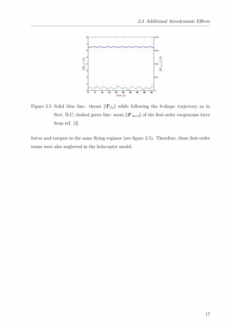
Figure 2.5: Solid blue line: thrust ‖T P1‖ while following the 8-shape trajectory as in
Sect. II.C; dashed green line: norm ‖F Aero‖ of the first-order exogenouse force
from ref. [3].
forces and torques in the same flying regimes (see figure 2.5). Therefore, these first-order
terms were also neglected in the holocopter model.
17
Chapter 2 Dynamical Model of the Holocopter
Symbols Definitions
ρ [kg/m3] Air density
A [m2] Propeller disk area
v1 [m/s] Propeller inflow velocity
FH [N ] Hub force
τR [Nm] Rolling moment
R [m] Propeller radius
a Lift slope
σ [rad−1] Solidity ratio
Cd Average drag coefficient
λi Inflow ratio
µi Rotor advance ratio
θ0 [rad] Pitch of incidence
θtw [rad] Twist pitch
xPi, yPi
, zPi[m/s] Velocity of the propeller w.r.t. ground
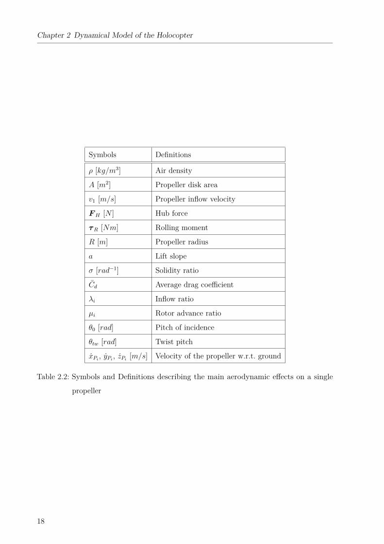
Table 2.2: Symbols and Definitions describing the main aerodynamic effects on a single
propeller
18
Chapter 3
Motion Control of the Holocopter
This chapter has been mainly reproduced from an article published in ICRA 2012: Ryll
et al. (2012)
We start with some preliminary considerations: the dynamic model illustrated in the
previous Section is useful for simulation purposes as it captures the main effects of the
quadrotor motion in space (apart from unmodeled aerodynamics forces and torques). Some
simplifications are however useful for transforming it into a ‘reduced model’ more suited to
control design. First, as in many practical situations, we assume that the motors actuating
the tilting/spinning axes are implementing a fast high-gain local controller able to impose
desired speeds wαi= αi and wi with negligible transients1. This allows to neglect the motor
dynamics, and to consider wαiand wi, i = 1 . . . 4, as (virtual) control inputs in place of the
motor torques ταiand τwi
. Second, in this simplified model we also neglect the internal
gyroscopic/inertial effects by considering them as second-order disturbances to be rejected
by the controller2. We note that the validity of these assumptions will be discussed in
Sect. 5.1 where the proposed controller will be tested against the complete dynamic model
of Sect. 2 representing the actual dynamics of the quadrotor.
Let us then define α = [α1 . . . α4]T ∈ R4, wα = [wα1 . . . wα4 ]T ∈ R4 and w =
[w1|w1| . . . w4|w4|]T ∈ R4. Note that the elements of vector w are the signed squares
of the spinning velocities wi, as the torques and forces in (2.2)–(2.3) are a (approx. linear)1For instance, in the standard quadrotor case, the spinning velocities wi are usually taken as control
inputs.2Obviously, this assumption holds as long as the inertia of the propeller group is small w.r.t. the main
holocopter body.
19
Chapter 3 Motion Control of the Holocopter
function of these quantities. Therefore, in the following analysis, wi = wi|wi| will be
considered as input ‘spinning velocity’ of the i-th propeller, with the understanding that
one can always recover the actual speed wi = sign(wi)√|wi|. Under the stated assumptions,
the quadrotor dynamic model can be simplified into
p =
0
0
−g
+ 1m
WRBF (α)w
ωB = I−1B τ (α)w
α = wα
WRB = WRB[ωB]∧
(3.1)
with [·]∧ being the usual map taking a vector a ∈ R3 into the associated skew-symmetric
matrix [a]× ∈ so(3), and
F (α) =
0 −kfs2 0 kfs4
−kfs1 0 kfs3 0
kfc1 −kfc2 kfc3 −kfc4
,
τ (α) =
0 −Lkfc2 − kms2
−Lkfc1 + kms1 0
−Lkfs1 − kmc1 Lkfs2 − kmc2
0 Lkfc4 + kms4
Lkfc3 − kms3 0
−Lkfs3 − kmc3 Lkfs4 − kmc4
(3.2)
the 3 × 4 input coupling matrixes (si = sin(αi) and ci = cos(αi)). Note that input w
appears linearly in (3.1) as expected. The subsequent control design is then performed on
the simplified model (3.1–3.2).
3.1 Control Design
The control problem considered in this thesis is an output tracking problem: how to track,
with the available inputs, a desired (and arbitrary) trajectory (pd(t), Rd(t)) ∈ R3 × SO(3)
20
3.1 Control Design
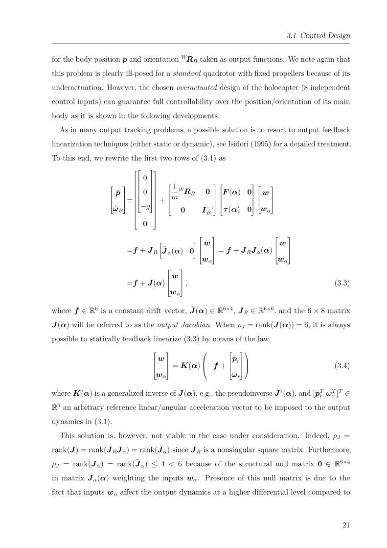
for the body position p and orientation WRB taken as output functions. We note again that
this problem is clearly ill-posed for a standard quadrotor with fixed propellers because of its
underactuation. However, the chosen overactuated design of the holocopter (8 independent
control inputs) can guarantee full controllability over the position/orientation of its main
body as it is shown in the following developments.
As in many output tracking problems, a possible solution is to resort to output feedback
linearization techniques (either static or dynamic), see Isidori (1995) for a detailed treatment.
To this end, we rewrite the first two rows of (3.1) as
pωB
=
0
0
−g
0
+
1m
WRB 0
0 I−1B
F (α) 0
τ (α) 0
wwα
=f + JR[Jα(α) 0
] wwα
= f + JRJα(α)
wwα
=f + J(α)
wwα
, (3.3)
where f ∈ R6 is a constant drift vector, J(α) ∈ R6×4, JR ∈ R6×6, and the 6 × 8 matrix
J(α) will be referred to as the output Jacobian. When ρJ = rank(J(α)) = 6, it is always
possible to statically feedback linearize (3.3) by means of the lawwwα
= K(α)
−f +
prωr
(3.4)
whereK(α) is a generalized inverse of J(α), e.g., the pseudoinverse J †(α), and [pTr ωTr ]T ∈
R6 an arbitrary reference linear/angular acceleration vector to be imposed to the output
dynamics in (3.1).
This solution is, however, not viable in the case under consideration. Indeed, ρJ =
rank(J) = rank(JRJα) = rank(Jα) since JR is a nonsingular square matrix. Furthermore,
ρJ = rank(Jα) = rank(Jα) ≤ 4 < 6 because of the structural null matrix 0 ∈ R6×4
in matrix Jα(α) weighting the inputs wα. Presence of this null matrix is due to the
fact that inputs wα affect the output dynamics at a higher differential level compared to
21
Chapter 3 Motion Control of the Holocopter
inputs w. Therefore, a direct inversion at the acceleration level is bound to exploit only
inputs w resulting in a loss of controllability for the system. Intuitively, the instantaneous
linear/angular acceleration of the quadrotor body is directly affected by the propeller speeds
w and tilting configuration α (thanks to the dependence in Jα(α)), but not by α = wα,
i.e., the tilting velocities3.
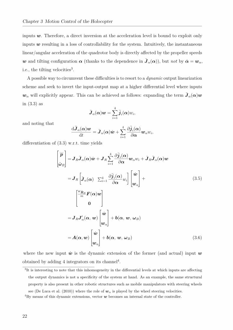
A possible way to circumvent these difficulties is to resort to a dynamic output linearization
scheme and seek to invert the input-output map at a higher differential level where inputs
wα will explicitly appear. This can be achieved as follows: expanding the term Jα(α)w
in (3.3) as
Jα(α)w =4∑i=1ji(α)wi,
and noting thatdJα(α)w
dt = Jα(α)w +4∑i=1
∂ji(α)∂α
wαwi,
differentiation of (3.3) w.r.t. time yields ...pωB
=JRJα(α)w + JR4∑i=1
∂ji(α)∂α
wαwi + JRJα(α)w
=JR[Jα(α) ∑4
i=1∂ji(α)∂α
wi
] wwα
+ (3.5)
WRB
mF (α)w
0
=JRJ ′α(α, w)
wwα
+ b(α, w, ωB)
=A(α,w)
wwα
+ b(α, w, ωB) (3.6)
where the new input w is the dynamic extension of the former (and actual) input w
obtained by adding 4 integrators on its channel4.3It is interesting to note that this inhomogeneity in the differential levels at which inputs are affecting
the output dynamics is not a specificity of the system at hand. As an example, the same structural
property is also present in other robotic structures such as mobile manipulators with steering wheels
see (De Luca et al. (2010)) where the role of wα is played by the wheel steering velocities.4By means of this dynamic extensions, vector w becomes an internal state of the controller.
22
3.1 Control Design
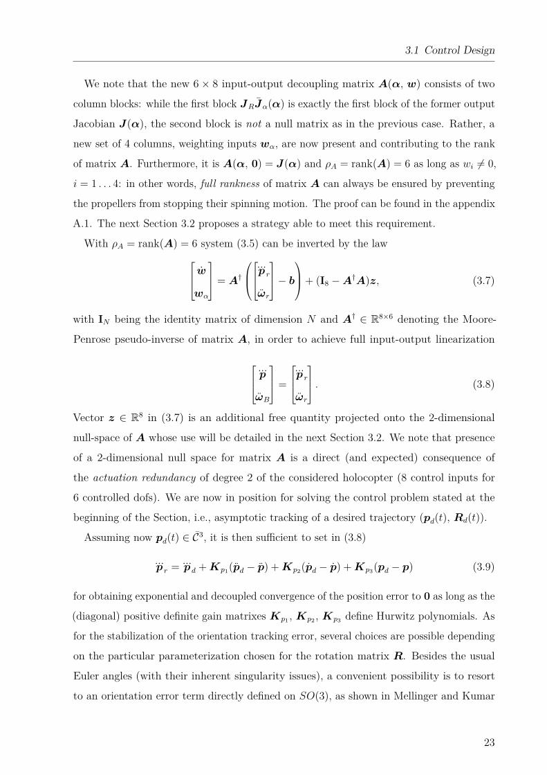
We note that the new 6 × 8 input-output decoupling matrix A(α, w) consists of two
column blocks: while the first block JRJα(α) is exactly the first block of the former output
Jacobian J(α), the second block is not a null matrix as in the previous case. Rather, a
new set of 4 columns, weighting inputs wα, are now present and contributing to the rank
of matrix A. Furthermore, it is A(α, 0) = J(α) and ρA = rank(A) = 6 as long as wi 6= 0,
i = 1 . . . 4: in other words, full rankness of matrix A can always be ensured by preventing
the propellers from stopping their spinning motion. The proof can be found in the appendix
A.1. The next Section 3.2 proposes a strategy able to meet this requirement.
With ρA = rank(A) = 6 system (3.5) can be inverted by the law wwα
= A†
...p rωr
− b+ (I8 −A†A)z, (3.7)
with IN being the identity matrix of dimension N and A† ∈ R8×6 denoting the Moore-
Penrose pseudo-inverse of matrix A, in order to achieve full input-output linearization
...pωB
=
...p rωr
. (3.8)
Vector z ∈ R8 in (3.7) is an additional free quantity projected onto the 2-dimensional
null-space of A whose use will be detailed in the next Section 3.2. We note that presence
of a 2-dimensional null space for matrix A is a direct (and expected) consequence of
the actuation redundancy of degree 2 of the considered holocopter (8 control inputs for
6 controlled dofs). We are now in position for solving the control problem stated at the
beginning of the Section, i.e., asymptotic tracking of a desired trajectory (pd(t), Rd(t)).
Assuming now pd(t) ∈ C3, it is then sufficient to set in (3.8)
...p r = ...
pd +Kp1(pd − p) +Kp2(pd − p) +Kp3(pd − p) (3.9)
for obtaining exponential and decoupled convergence of the position error to 0 as long as the
(diagonal) positive definite gain matrixes Kp1 , Kp2 , Kp3 define Hurwitz polynomials. As
for the stabilization of the orientation tracking error, several choices are possible depending
on the particular parameterization chosen for the rotation matrix R. Besides the usual
Euler angles (with their inherent singularity issues), a convenient possibility is to resort
to an orientation error term directly defined on SO(3), as shown in Mellinger and Kumar
23
Chapter 3 Motion Control of the Holocopter
(2011) and Lee et al. (2010). Assume, as before, that Rd(t) ∈ C3 and let ωd = [RTd Rd]∨,
where [·]∨ represents the inverse map from so(3) to R3. By defining the orientation error as
eR = 12[WRT
BRd −RTdWRB]∨ (3.10)
the choice
ωr = ωd +Kω1(ωd − ωB) +Kω2(ωd − ωB) +Kω3eR (3.11)
in (3.8) yields an exponential convergence for the orientation tracking error to 0 as desired,
provided that the (diagonal) gain matrixes Kω1 , Kω2 , Kω3 define a Hurwitz polynomial.
3.2 Optimization of Additional Criteria
As a final step, we now discuss how to exploit the 2-dimensional actuation redundancy of
the holocopter by exploiting vector z in (3.7).
Being projected onto the null space of A, vector z does not produce actions interfering
with the output tracking objective and can thus be exploited to fulfill additional tasks.
In our case, a first mandatory requirement is to keep ρA = 6 at all times for avoiding
singularities of the decoupling matrix A in (3.7). As explained, this objective can be easily
met by ensuring w 6= 0. Likewise another important requirement is to minimize the norm
of w in order to reduce the energy consumption during flight since, for instance, the air
drag torques τ exti in (2.2) are always performing a dissipative work against wi.
A possible cost function H(w) taking into account these two competing objectives is
H(w) =4∑i=1
h(wi)
with
h(wi) =
kh1 tan2(γ1|wi|+ γ2) wmin < |wi| ≤ wrest
kh2(|wi| − wrest)2 |wi| > wrest
, (3.12)
γ1 = π2(wrest−wmin) , γ2 = −γ1wrest, and kh1 > 0, kh2 > 0 suitable scalar gains. Here, wmin > 0
represents a minimum value for the propeller spinning velocities and wrest > wmin a suitable
‘rest’ speed. Furthermore, functions hi(wi) are such that hi(wi)→∞ if either |wi| → wmin
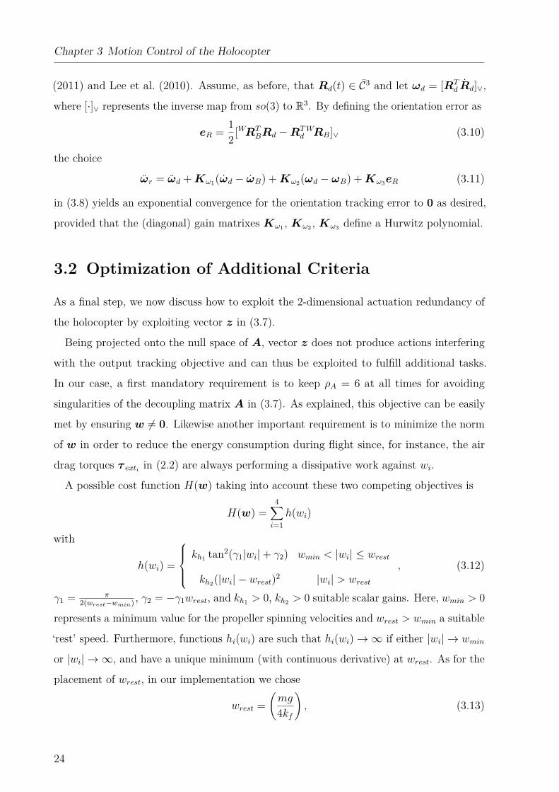
or |wi| → ∞, and have a unique minimum (with continuous derivative) at wrest. As for the
placement of wrest, in our implementation we chose
wrest =(mg
4kf
), (3.13)
24
3.2 Optimization of Additional Criteria
0 0.5 1 1.5 2 2.5 3 3.5 4
x 105
0
0.5
1
1.5
2
2.5
3
3.5
4x 10
11
hi(w
i)
|wi| [rad2/s2]
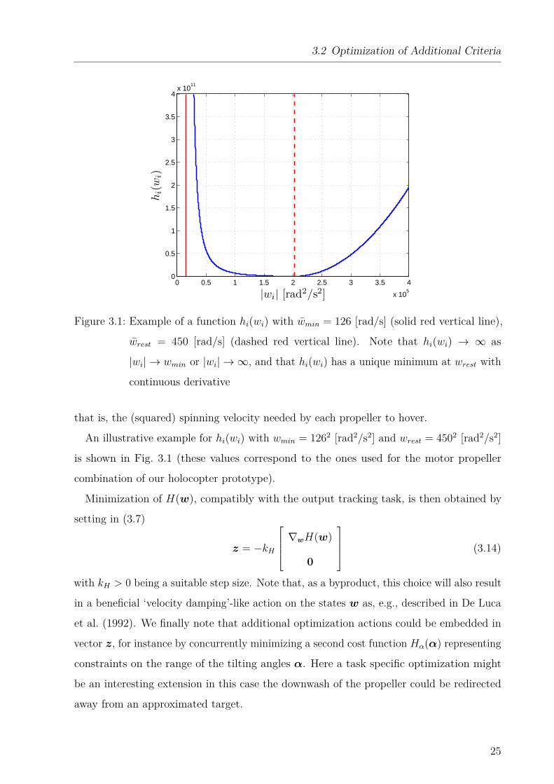
Figure 3.1: Example of a function hi(wi) with wmin = 126 [rad/s] (solid red vertical line),
wrest = 450 [rad/s] (dashed red vertical line). Note that hi(wi) → ∞ as
|wi| → wmin or |wi| → ∞, and that hi(wi) has a unique minimum at wrest with
continuous derivative
that is, the (squared) spinning velocity needed by each propeller to hover.
An illustrative example for hi(wi) with wmin = 1262 [rad2/s2] and wrest = 4502 [rad2/s2]
is shown in Fig. 3.1 (these values correspond to the ones used for the motor propeller
combination of our holocopter prototype).
Minimization of H(w), compatibly with the output tracking task, is then obtained by
setting in (3.7)
z = −kH
∇wH(w)
0
(3.14)
with kH > 0 being a suitable step size. Note that, as a byproduct, this choice will also result
in a beneficial ‘velocity damping’-like action on the states w as, e.g., described in De Luca
et al. (1992). We finally note that additional optimization actions could be embedded in
vector z, for instance by concurrently minimizing a second cost function Hα(α) representing
constraints on the range of the tilting angles α. Here a task specific optimization might
be an interesting extension in this case the downwash of the propeller could be redirected
away from an approximated target.
25
Chapter 3 Motion Control of the Holocopter
3.2.1 Dynamic adaptation of wrest
The optimization as introduced in Sect. 3.2 guarantees a minimum energy consumption
under a non-dynamic flight regime (p = 0). In this case the internal forces are minimized.
Under a dynamic fight regime (p 6= 0) this is not given as the constant value of wrest is
determined as in (3.13), which is the minimum value for hovering condition but not the
minimum value for a desired acceleration p. Therefore the determination of the term wrest
can be extended by a dynamical term describing the currently desired vertical acceleration
wrest =
(m
4kf(g + pz)
)kswmin ≤ wrest
kswmin = wrest kswmin > wrest
, (3.15)
with pz being the z-component of the desired acceleration pd in (3.9) and ks being a
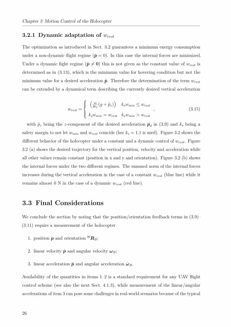
safety margin to not let wmin and wrest coincide (her ks = 1.1 is used). Figure 3.2 shows the
different behavior of the holocopter under a constant and a dynamic control of wrest. Figure
3.2 (a) shows the desired trajectory for the vertical position, velocity and acceleration while
all other values remain constant (position in x and y and orientation). Figure 3.2 (b) shows
the internal forces under the two different regimes. The summed norm of the internal forces
increases during the vertical acceleration in the case of a constant wrest (blue line) while it
remains almost 0 N in the case of a dynamic wrest (red line).
3.3 Final Considerations
We conclude the section by noting that the position/orientation feedback terms in (3.9)–
(3.11) require a measurement of the holocopter
1. position p and orientation WRB;
2. linear velocity p and angular velocity ωB;
3. linear acceleration p and angular acceleration ωB.
Availability of the quantities in items 1–2 is a standard requirement for any UAV flight
control scheme (see also the next Sect. 4.1.3), while measurement of the linear/angular
accelerations of item 3 can pose some challenges in real-world scenarios because of the typical
26
3.3 Final Considerations
1 1.5 2 2.5 3 3.5 4 4.5 5−1
−0.5
0
pzd[m
]
time [s]
1 1.5 2 2.5 3 3.5 4 4.5 5−5
0
5
pzd[ms]
time [s]
1 1.5 2 2.5 3 3.5 4 4.5 5−10
0
10
pzd[m s2
]
time [s]
(a)
1 1.5 2 2.5 3 3.5 4 4.5 50
2
4
6
8
10
12
||Fint||[N
]
time [s]
(b)
Figure 3.2: (a): The desired trajectory is a movement along the z axis. The position in x
and y and the orientation remain constant. (b): Summed norm of the internal
forces: blue - constant wrest, red - dynamic wrest
high noise level of these signals when obtained from onboard sensors (e.g., accelerometers)
or numerical differentiation of velocity-like quantities.
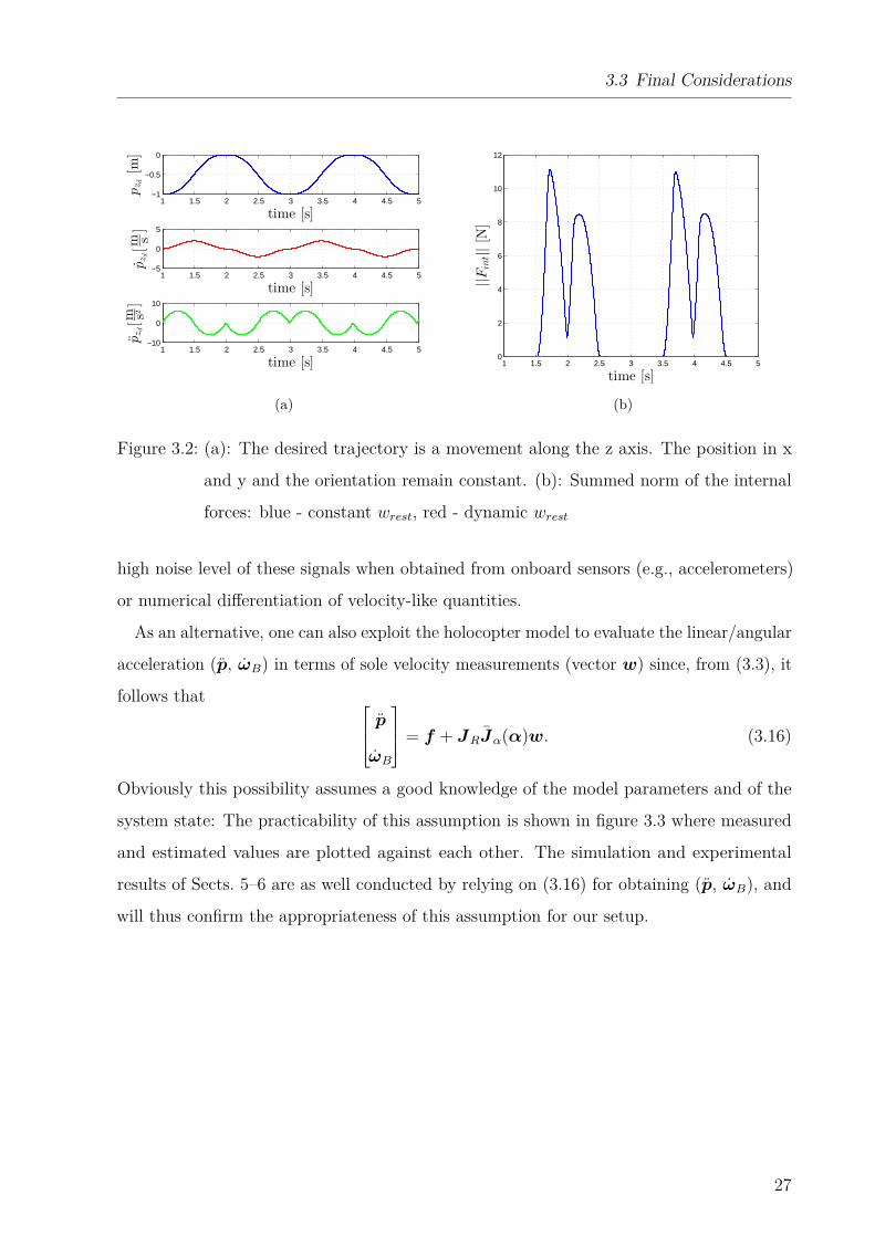
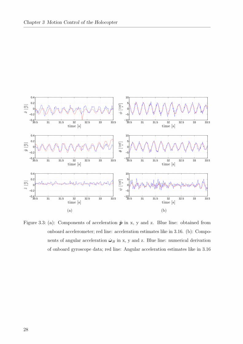
As an alternative, one can also exploit the holocopter model to evaluate the linear/angular
acceleration (p, ωB) in terms of sole velocity measurements (vector w) since, from (3.3), it
follows that pωB
= f + JRJα(α)w. (3.16)
Obviously this possibility assumes a good knowledge of the model parameters and of the
system state: The practicability of this assumption is shown in figure 3.3 where measured
and estimated values are plotted against each other. The simulation and experimental
results of Sects. 5–6 are as well conducted by relying on (3.16) for obtaining (p, ωB), and
will thus confirm the appropriateness of this assumption for our setup.
27
Chapter 3 Motion Control of the Holocopter
30.5 31 31.5 32 32.5 33 33.5−0.4
−0.2
0
0.2
0.4
x[m s
2]
time [s]30.5 31 31.5 32 32.5 33 33.5
−10
−5
0
5
10
φ[r
ad
s]
time [s]
30.5 31 31.5 32 32.5 33 33.5−0.4
−0.2
0
0.2
0.4
y[m s
2]
time [s]30.5 31 31.5 32 32.5 33 33.5
−10
−5
0
5
10
θ[r
ad
s]
time [s]
30.5 31 31.5 32 32.5 33 33.5−0.4
−0.2
0
0.2
0.4
z[m s
2]
time [s]
(a)
30.5 31 31.5 32 32.5 33 33.5−10
−5
0
5
10
ψ[r
ad
s]
time [s]
(b)
Figure 3.3: (a): Components of acceleration p in x, y and z. Blue line: obtained from
onboard accelerometer; red line: acceleration estimates like in 3.16. (b): Compo-
nents of angular acceleration ωB in x, y and z. Blue line: numerical derivation
of onboard gyroscope data; red line: Angular acceleration estimates like in 3.16
28
Chapter 4
Holocopter Prototype and System
Architecture
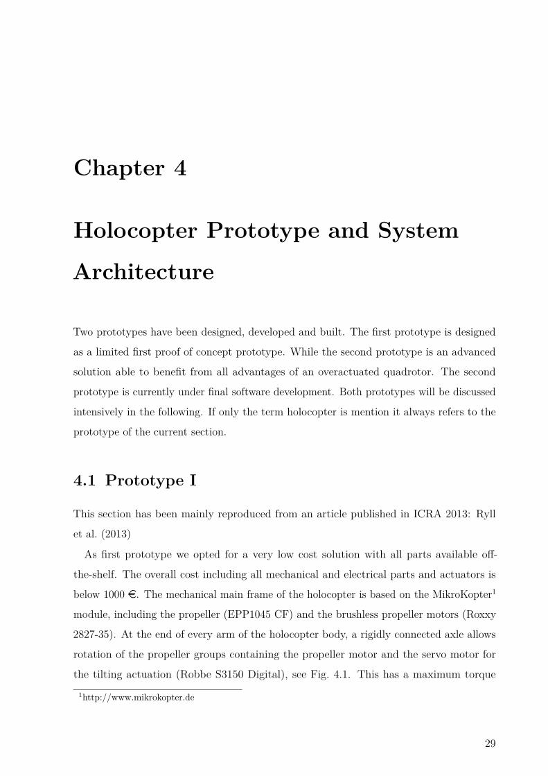
Two prototypes have been designed, developed and built. The first prototype is designed
as a limited first proof of concept prototype. While the second prototype is an advanced
solution able to benefit from all advantages of an overactuated quadrotor. The second
prototype is currently under final software development. Both prototypes will be discussed
intensively in the following. If only the term holocopter is mention it always refers to the
prototype of the current section.
4.1 Prototype I
This section has been mainly reproduced from an article published in ICRA 2013: Ryll
et al. (2013)
As first prototype we opted for a very low cost solution with all parts available off-
the-shelf. The overall cost including all mechanical and electrical parts and actuators is
below 1000 e. The mechanical main frame of the holocopter is based on the MikroKopter1
module, including the propeller (EPP1045 CF) and the brushless propeller motors (Roxxy
2827-35). At the end of every arm of the holocopter body, a rigidly connected axle allows
rotation of the propeller groups containing the propeller motor and the servo motor for
the tilting actuation (Robbe S3150 Digital), see Fig. 4.1. This has a maximum torque1http://www.mikrokopter.de
29
Chapter 4 Holocopter Prototype and System Architecture
Reflective markers
Servo motors
Brushless motor IMU board
Propeller group
Marker tree
Axle
Power-supply board
µC board
Brushless controllers
Q7-board
Battery
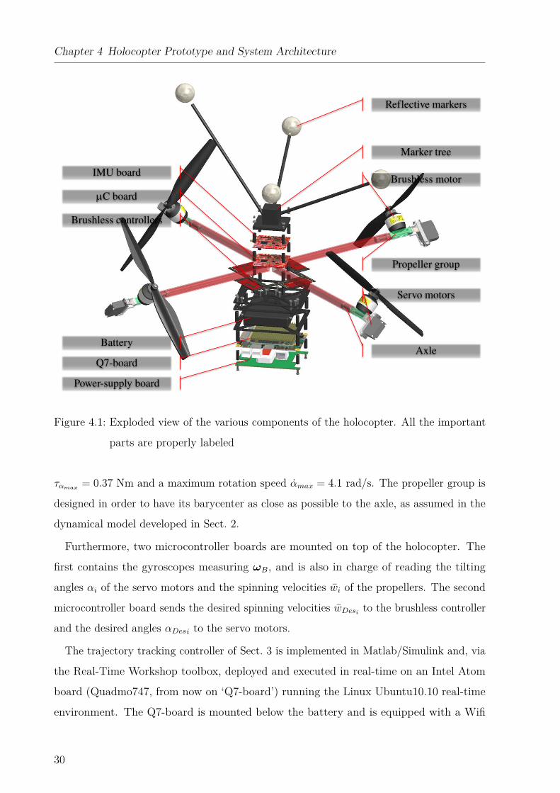
Figure 4.1: Exploded view of the various components of the holocopter. All the important
parts are properly labeled
ταmax = 0.37 Nm and a maximum rotation speed αmax = 4.1 rad/s. The propeller group is
designed in order to have its barycenter as close as possible to the axle, as assumed in the
dynamical model developed in Sect. 2.
Furthermore, two microcontroller boards are mounted on top of the holocopter. The
first contains the gyroscopes measuring ωB, and is also in charge of reading the tilting
angles αi of the servo motors and the spinning velocities wi of the propellers. The second
microcontroller board sends the desired spinning velocities wDesito the brushless controller
and the desired angles αDesi to the servo motors.
The trajectory tracking controller of Sect. 3 is implemented in Matlab/Simulink and, via
the Real-Time Workshop toolbox, deployed and executed in real-time on an Intel Atom
board (Quadmo747, from now on ‘Q7-board’) running the Linux Ubuntu10.10 real-time
environment. The Q7-board is mounted below the battery and is equipped with a Wifi
30

4.1 Prototype I
Figure 4.2: Illustrating snap shot series of the holocopter simulation. Holocopter performs
a rotation of π2 rad around x-axis. Please note the orientation of the propellers
during the maneuver
USB-dongle for communication. As only one RS-232 port (TTL level) is available on the
Q7-board, the second microcontroller board is connected via USB-port and an USBToSerial
converter. The Q7-board is powered by a battery, with the necessary voltage conversion
and stabilization performed by a power-supply board containing a 12V DC/DC power
converter.
The nominal mass of the full holocopter is 1.32 kg. From a high detail CAD model of
the body and propeller groups we also obtained the following inertia matrixes
IPi=
8.450e−5 0 0
0 8.450e−5 0
0 0 4.580e−5
[kg m2
]
and
IB =
0.0154 0 0
0 0.0154 0
0 0 0.0263
[kg m2
].
In the current setup, the servo motors are limited in their rotation by mechanical end stops
in the range of -90 deg < αi < 90 deg. For our particular prototype, these limits translate
into a maximum achievable rotation (in hover) of ≈ ±55 deg around the roll or pitch axes
for the body frame B (this value was experimentally determined) (Ryll et al. (2012)).
How the servo motor positions αi are changing over a main body rotation maneuver can be
seen in figure 4.2. The fourth holocopter from the left in the figure illustrates the maximum
achievable rotation for the prototype and the servo motors with −α1 = α3 ≈ 90 deg.
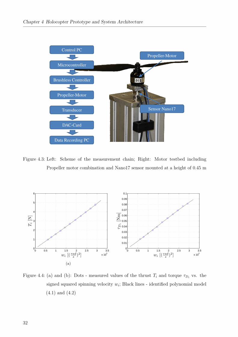
In order to obtain accurate values of kf and km for the used motor-propeller combination,
we made use of a testbed equipped with a 6-dof force/torque sensor (ATI Nano17-E, see
31
Chapter 4 Holocopter Prototype and System Architecture
Transducer
DAC-Card
Data Recording PC
Control PC
Microcontroller
Brushless Controller
Propeller-Motor
Sensor Nano17
Propeller-Motor
Figure 4.3: Left: Scheme of the measurement chain; Right: Motor testbed including
Propeller motor combination and Nano17 sensor mounted at a height of 0.45 m
0 0.5 1 1.5 2 2.5 3 3.5
x 105
0
1
2
3
4
5
6
Ti[N
]
wi [(rads )2]
(a)
0 0.5 1 1.5 2 2.5 3 3.5
x 105
0
0.01
0.02
0.03
0.04
0.05
0.06
0.07
0.08
0.09
0.1
τ Di[N
m]
wi [(rads )2]
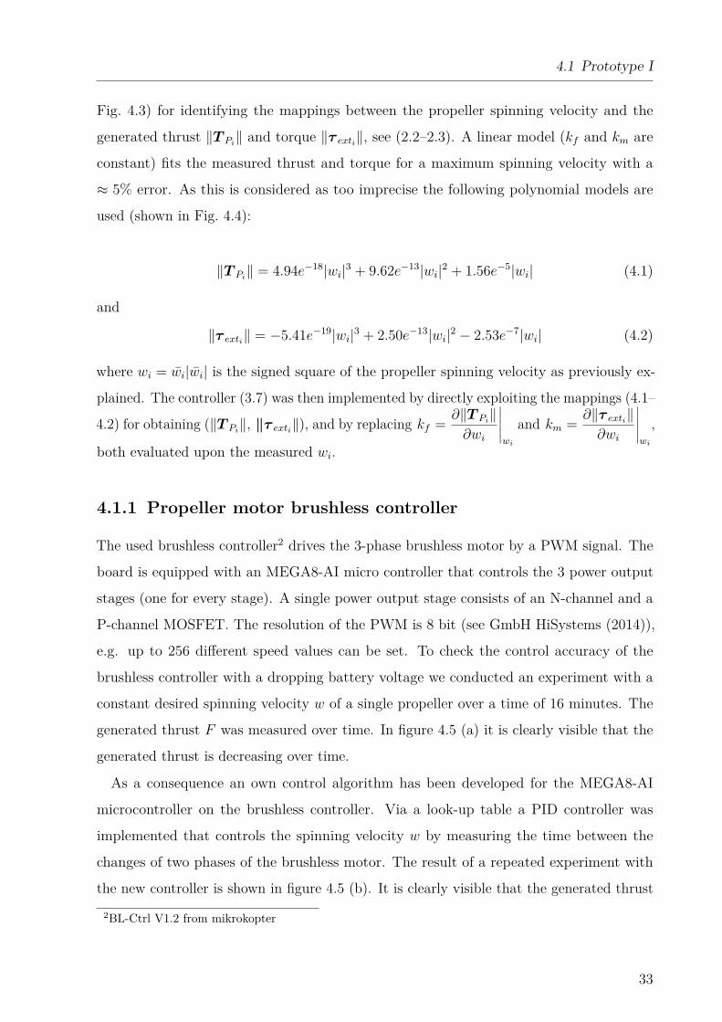
Figure 4.4: (a) and (b): Dots - measured values of the thrust Ti and torque τDivs. the
signed squared spinning velocity wi; Black lines - identified polynomial model
(4.1) and (4.2)
32
4.1 Prototype I
Fig. 4.3) for identifying the mappings between the propeller spinning velocity and the
generated thrust ‖T Pi‖ and torque ‖τ exti‖, see (2.2–2.3). A linear model (kf and km are
constant) fits the measured thrust and torque for a maximum spinning velocity with a
≈ 5% error. As this is considered as too imprecise the following polynomial models are
used (shown in Fig. 4.4):
‖T Pi‖ = 4.94e−18|wi|3 + 9.62e−13|wi|2 + 1.56e−5|wi| (4.1)
and
‖τ exti‖ = −5.41e−19|wi|3 + 2.50e−13|wi|2 − 2.53e−7|wi| (4.2)
where wi = wi|wi| is the signed square of the propeller spinning velocity as previously ex-
plained. The controller (3.7) was then implemented by directly exploiting the mappings (4.1–
4.2) for obtaining (‖T Pi‖, ‖τ exti‖), and by replacing kf = ∂‖T Pi
‖∂wi
∣∣∣∣∣wi
and km = ∂‖τ exti‖∂wi
∣∣∣∣∣wi
,
both evaluated upon the measured wi.
4.1.1 Propeller motor brushless controller
The used brushless controller2 drives the 3-phase brushless motor by a PWM signal. The
board is equipped with an MEGA8-AI micro controller that controls the 3 power output
stages (one for every stage). A single power output stage consists of an N-channel and a
P-channel MOSFET. The resolution of the PWM is 8 bit (see GmbH HiSystems (2014)),
e.g. up to 256 different speed values can be set. To check the control accuracy of the
brushless controller with a dropping battery voltage we conducted an experiment with a
constant desired spinning velocity w of a single propeller over a time of 16 minutes. The
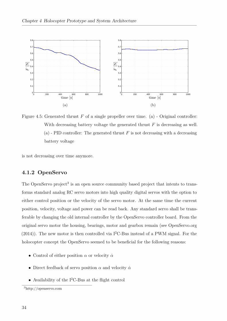
generated thrust F was measured over time. In figure 4.5 (a) it is clearly visible that the
generated thrust is decreasing over time.
As a consequence an own control algorithm has been developed for the MEGA8-AI
microcontroller on the brushless controller. Via a look-up table a PID controller was
implemented that controls the spinning velocity w by measuring the time between the
changes of two phases of the brushless motor. The result of a repeated experiment with
the new controller is shown in figure 4.5 (b). It is clearly visible that the generated thrust2BL-Ctrl V1.2 from mikrokopter
33
Chapter 4 Holocopter Prototype and System Architecture
0 200 400 600 800 10005
5.1
5.2
5.3
5.4
5.5
5.6
5.7
5.8
F[N
]
time [s]
(a)
0 200 400 600 800 10005
5.1
5.2
5.3
5.4
5.5
5.6
5.7
5.8
F[N
]
time [s]
(b)
Figure 4.5: Generated thrust F of a single propeller over time. (a) - Original controller:
With decreasing battery voltage the generated thrust F is decreasing as well.
(a) - PID controller: The generated thrust F is not decreasing with a decreasing
battery voltage
is not decreasing over time anymore.
4.1.2 OpenServo
The OpenServo project3 is an open source community based project that intents to trans-
forms standard analog RC servo motors into high quality digital servos with the option to
either control position or the velocity of the servo motor. At the same time the current
position, velocity, voltage and power can be read back. Any standard servo shall be trans-
ferable by changing the old internal controller by the OpenServo controller board. From the
original servo motor the housing, bearings, motor and gearbox remain (see OpenServo.org
(2014)). The new motor is then controlled via I2C-Bus instead of a PWM signal. For the
holocopter concept the OpenServo seemed to be beneficial for the following reasons:
• Control of either position α or velocity α
• Direct feedback of servo position α and velocity α
• Availability of the I2C-Bus at the flight control3http://openservo.com
34
4.1 Prototype I
• Shorter signal delay of I2C-Bus compared with PWM
• Higher control frequency (standard servos /approx50 Hz)
• Very lightweight
• Directly available and cheap solution
For a first test an OpenServo v2-module has been used combined with a Robbe s3150
servo motor. The results were very disappointing. A stable or accurate control could not
be achieved. Additionally in a final position the servo motor was still oscillating. Therefore
it was decided to not use the OpenServo-modules any more but directly the original Robbe
s3150 servo motors with a maximum torque of τmax = 0.046Nm and a maximum velocity
of αmax ≈ 4.133rads (see robbe Modellsport GmbH & Co. KG (2014)).
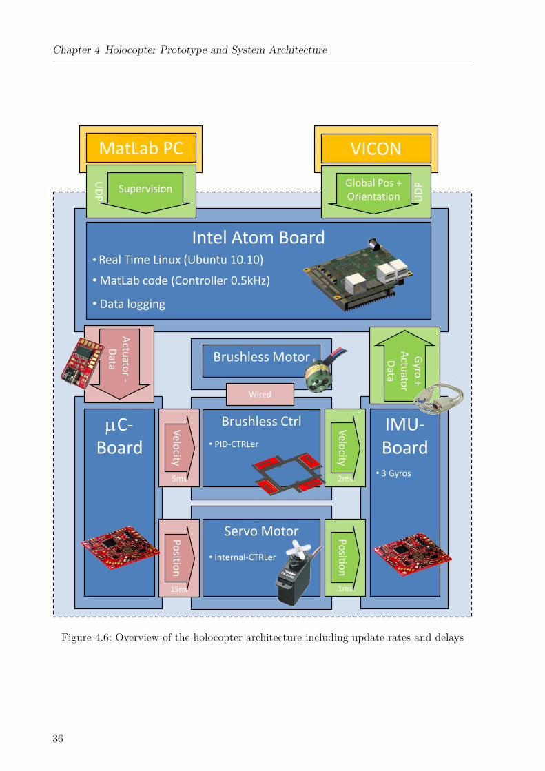
4.1.3 System architecture
The Q7-board runs a GNU-Linux Ubuntu 10.10 real time OS and executes the Matlab-
generated code. The controller runs at 500 Hz and takes as inputs: (i) the desired trajectory
(pd(t), Rd(t)) and needed derivatives (pd(t), pd(t),...pd(t)) and (ωd(t), ωd(t), ωd(t)), (ii)
the current position/orientation of the holocopter (p, WRB) and its linear/angular velocity
(p, ωB), (iii) the spinning velocities of the propellers wi, (iv) the tilting angles αi.
The position p and orientation WRB of the holocopter are directly obtained from an
external motion capture system4 (MoCap) at 200 Hz. A marker tree consisting of five
infra-red markers is mounted on top of the holocopter for this purpose. Knowing p, the
linear velocity p is then obtained via numerical differentiation, while the angular velocity
ωB is measured by the onboard IMU (3 ADXRS610 gyroscopes).
Due to performance reasons (bottleneck in serial communication), the sending of the
desired motor speeds and tilting angles, and the reading of the IMU-data, of the actual
spinning velocities, and of tilting angles is split among two communication channels and
two microcontrollers (called, from now on, ‘µC-Board’ and ‘IMU-Board’). The desired
motor spinning velocities wDesiare sent from the Q7-board to the µC-Board via a serial
connection at the frequency of 250 Hz and 8 bit resolution, and from the µC-Board to the4http://www.vicon.com/products/bonita.html
35
Chapter 4 Holocopter Prototype and System Architecture
Intel Atom Board
• Real Time Linux (Ubuntu 10.10)
• MatLab code (Controller 0.5kHz)
• Data logging
VICON
UD
P Global Pos + Orientation
IMU-Board
• 3 Gyros
µC-Board
Gyro +
Actuator D
ata
Actuator -
Data
Servo Motor
• Internal-CTRLer
Brushless Ctrl
• PID-CTRLer
Brushless Motor
Wired
15ms
5ms
1ms
2ms
Velocity Position
Position Velocity
MatLab PC
UD
P
Supervision
Figure 4.6: Overview of the holocopter architecture including update rates and delays
36
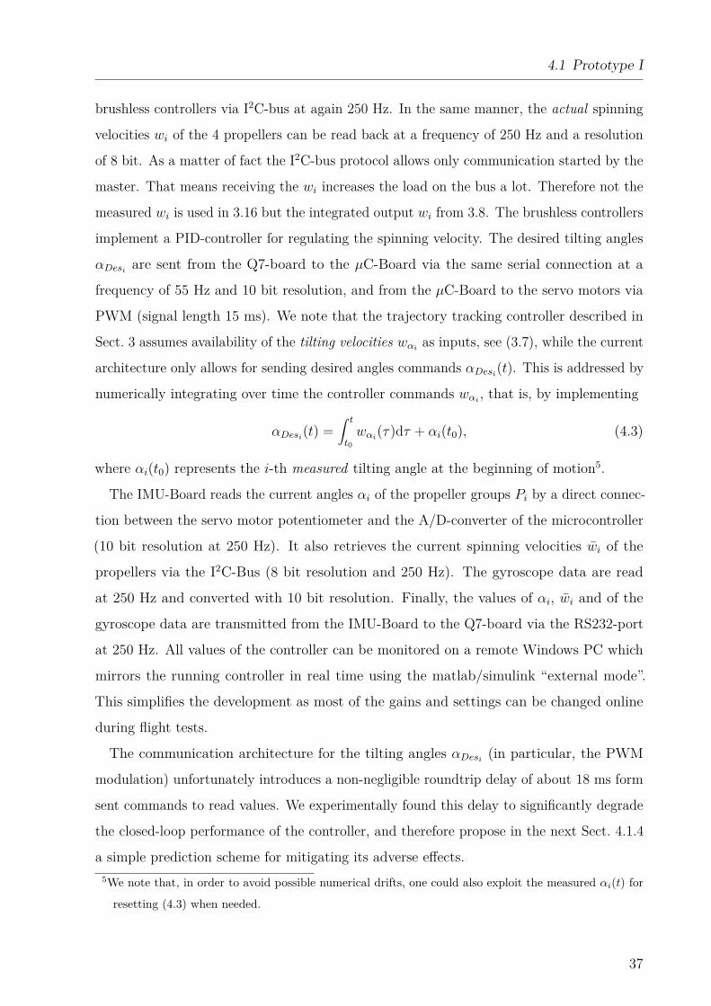
4.1 Prototype I
brushless controllers via I2C-bus at again 250 Hz. In the same manner, the actual spinning
velocities wi of the 4 propellers can be read back at a frequency of 250 Hz and a resolution
of 8 bit. As a matter of fact the I2C-bus protocol allows only communication started by the
master. That means receiving the wi increases the load on the bus a lot. Therefore not the
measured wi is used in 3.16 but the integrated output wi from 3.8. The brushless controllers
implement a PID-controller for regulating the spinning velocity. The desired tilting angles
αDesiare sent from the Q7-board to the µC-Board via the same serial connection at a
frequency of 55 Hz and 10 bit resolution, and from the µC-Board to the servo motors via
PWM (signal length 15 ms). We note that the trajectory tracking controller described in
Sect. 3 assumes availability of the tilting velocities wαias inputs, see (3.7), while the current
architecture only allows for sending desired angles commands αDesi(t). This is addressed by
numerically integrating over time the controller commands wαi, that is, by implementing
αDesi(t) =
∫ t
t0wαi
(τ)dτ + αi(t0), (4.3)
where αi(t0) represents the i-th measured tilting angle at the beginning of motion5.
The IMU-Board reads the current angles αi of the propeller groups Pi by a direct connec-
tion between the servo motor potentiometer and the A/D-converter of the microcontroller
(10 bit resolution at 250 Hz). It also retrieves the current spinning velocities wi of the
propellers via the I2C-Bus (8 bit resolution and 250 Hz). The gyroscope data are read
at 250 Hz and converted with 10 bit resolution. Finally, the values of αi, wi and of the
gyroscope data are transmitted from the IMU-Board to the Q7-board via the RS232-port
at 250 Hz. All values of the controller can be monitored on a remote Windows PC which
mirrors the running controller in real time using the matlab/simulink “external mode”.
This simplifies the development as most of the gains and settings can be changed online
during flight tests.
The communication architecture for the tilting angles αDesi(in particular, the PWM
modulation) unfortunately introduces a non-negligible roundtrip delay of about 18 ms form
sent commands to read values. We experimentally found this delay to significantly degrade
the closed-loop performance of the controller, and therefore propose in the next Sect. 4.1.4
a simple prediction scheme for mitigating its adverse effects.5We note that, in order to avoid possible numerical drifts, one could also exploit the measured αi(t) for
resetting (4.3) when needed.
37
Chapter 4 Holocopter Prototype and System Architecture
2 2. 5 3 3. 5 4 4. 5 5 5. 5 6−10
0
10
20
30
40
50
time [s]
α[deg]
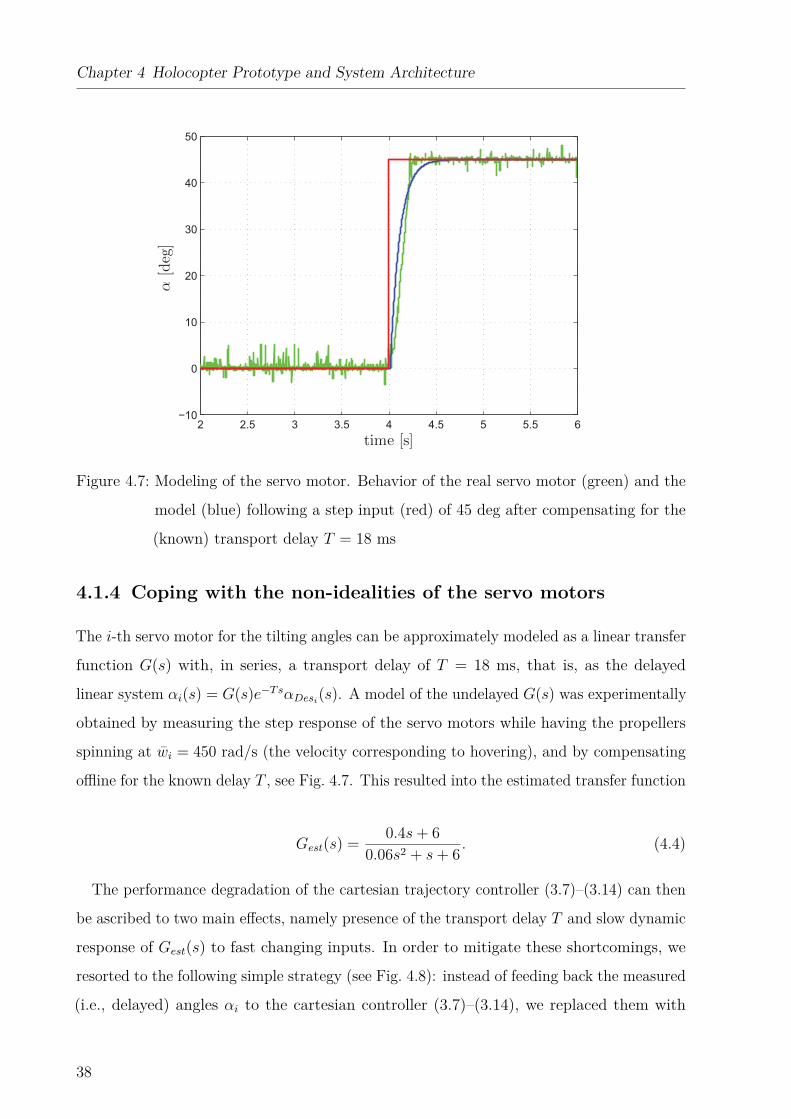
Figure 4.7: Modeling of the servo motor. Behavior of the real servo motor (green) and the
model (blue) following a step input (red) of 45 deg after compensating for the
(known) transport delay T = 18 ms
4.1.4 Coping with the non-idealities of the servo motors
The i-th servo motor for the tilting angles can be approximately modeled as a linear transfer
function G(s) with, in series, a transport delay of T = 18 ms, that is, as the delayed
linear system αi(s) = G(s)e−TsαDesi(s). A model of the undelayed G(s) was experimentally
obtained by measuring the step response of the servo motors while having the propellers
spinning at wi = 450 rad/s (the velocity corresponding to hovering), and by compensating
offline for the known delay T , see Fig. 4.7. This resulted into the estimated transfer function
Gest(s) = 0.4s+ 60.06s2 + s+ 6 . (4.4)
The performance degradation of the cartesian trajectory controller (3.7)–(3.14) can then
be ascribed to two main effects, namely presence of the transport delay T and slow dynamic
response of Gest(s) to fast changing inputs. In order to mitigate these shortcomings, we
resorted to the following simple strategy (see Fig. 4.8): instead of feeding back the measured
(i.e., delayed) angles αi to the cartesian controller (3.7)–(3.14), we replaced them with
38
4.1 Prototype I
Servo-Motor
Servo-Model
Delay
Controller αi Des
Cartesian Controller αi
Filter
+ -
-
+ +
+
αi Real
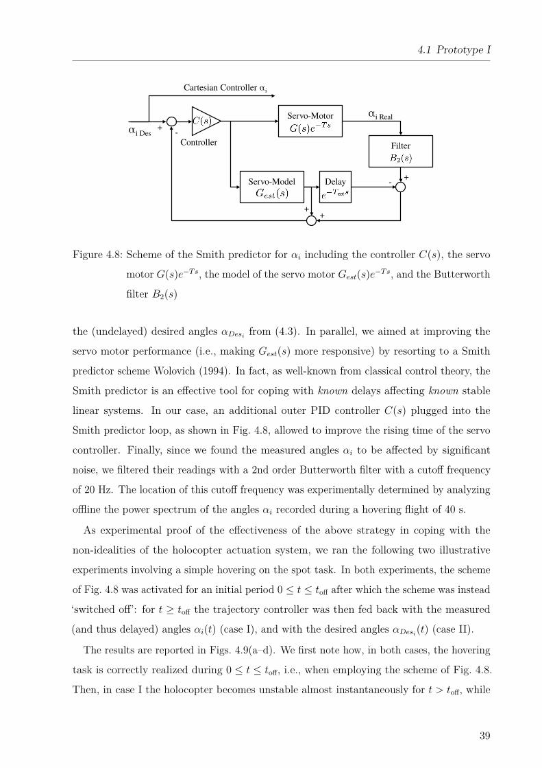
Figure 4.8: Scheme of the Smith predictor for αi including the controller C(s), the servo
motor G(s)e−Ts, the model of the servo motor Gest(s)e−Ts, and the Butterworth
filter B2(s)
the (undelayed) desired angles αDesifrom (4.3). In parallel, we aimed at improving the
servo motor performance (i.e., making Gest(s) more responsive) by resorting to a Smith
predictor scheme Wolovich (1994). In fact, as well-known from classical control theory, the
Smith predictor is an effective tool for coping with known delays affecting known stable
linear systems. In our case, an additional outer PID controller C(s) plugged into the
Smith predictor loop, as shown in Fig. 4.8, allowed to improve the rising time of the servo
controller. Finally, since we found the measured angles αi to be affected by significant
noise, we filtered their readings with a 2nd order Butterworth filter with a cutoff frequency
of 20 Hz. The location of this cutoff frequency was experimentally determined by analyzing
offline the power spectrum of the angles αi recorded during a hovering flight of 40 s.
As experimental proof of the effectiveness of the above strategy in coping with the
non-idealities of the holocopter actuation system, we ran the following two illustrative
experiments involving a simple hovering on the spot task. In both experiments, the scheme
of Fig. 4.8 was activated for an initial period 0 ≤ t ≤ toff after which the scheme was instead
‘switched off’: for t ≥ toff the trajectory controller was then fed back with the measured
(and thus delayed) angles αi(t) (case I), and with the desired angles αDesi(t) (case II).
The results are reported in Figs. 4.9(a–d). We first note how, in both cases, the hovering
task is correctly realized during 0 ≤ t ≤ toff, i.e., when employing the scheme of Fig. 4.8.
Then, in case I the holocopter becomes unstable almost instantaneously for t > toff, while
39
Chapter 4 Holocopter Prototype and System Architecture
60 60.5 61 61.5 62 62.5 63 63.5 64 64.5−1
−0.8
−0.6
−0.4
−0.2
0
0.2
0.4
0.6
0.8
1
α[rad]
time [s]
(a)
60 60.5 61 61.5 62 62.5 63 63.5 64 64.5−0.1
−0.08
−0.06
−0.04
−0.02
0
0.02
0.04
0.06
0.08
0.1
eP[m
]time [s]
(b)
25 30 35 40 45 50 55−1
−0.8
−0.6
−0.4
−0.2
0
0.2
0.4
0.6
0.8
1
α[rad]
time [s]
(c)
25 30 35 40 45 50 55−0.1
−0.08
−0.06
−0.04
−0.02
0
0.02
0.04
0.06
0.08
0.1
eP[m
]
time [s]
(d)
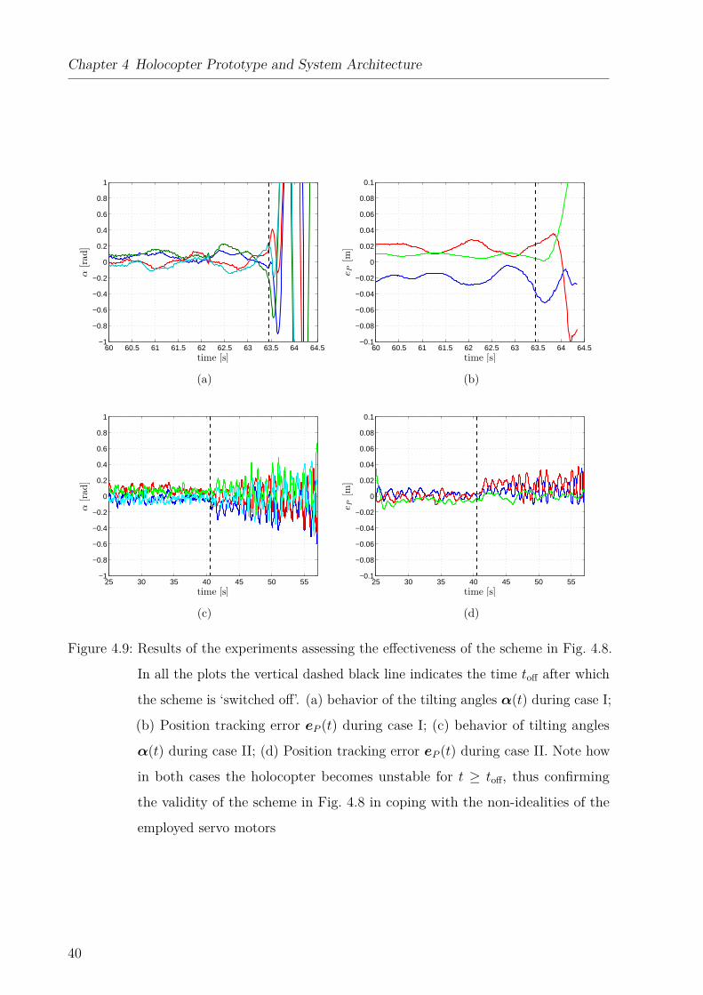
Figure 4.9: Results of the experiments assessing the effectiveness of the scheme in Fig. 4.8.
In all the plots the vertical dashed black line indicates the time toff after which
the scheme is ‘switched off’. (a) behavior of the tilting angles α(t) during case I;
(b) Position tracking error eP (t) during case I; (c) behavior of tilting angles
α(t) during case II; (d) Position tracking error eP (t) during case II. Note how
in both cases the holocopter becomes unstable for t ≥ toff, thus confirming
the validity of the scheme in Fig. 4.8 in coping with the non-idealities of the
employed servo motors
40
4.2 Prototype II
in case II the servo motors start to slowly oscillate to then reach practical instability at
about t > toff + 15 s. These results allow us to then conclude the ability of the proposed
strategy to cope with the shortcomings of the holocopter actuation system.
4.2 Prototype II
4.2.1 Mechanical design
After very promising experiments (see section 6) with the first prototype it has been decided
to design and build a second prototype based on the experiences of the first holocopter.
Based on simulations the low control rate and especially the communication delay of the
servo motor have been identified as the bottleneck of precise position and orientation
tracking of the first prototype (see section 5.2.3). Furthermore, a list of requirements has
been defined to additionally improve the holocopter:
• Revision of the servo motors
– Control frequency ≥ 200 Hz
– Communication send delay ≤ 5 ms
– Continuous rotation of the servo arm
• Reduction of weight by ≥ 20 %
• Reduction of inertia by ≥ 20 %
• Increase of computational power
• Center of gravity coincides with center of arm rotation
• Center of arm rotation in alignment with center of thrust and drag
To fulfill these requirements a complete redesign was necessary (see figure 4.10). To
achieve an alignment between the arm rotation and the center of generated thrust as well
as the center of gravity of the main body, it was mandatory to not let the propeller motors
directly rotate around their arms. Therefore the servo motors of the second prototype are
41
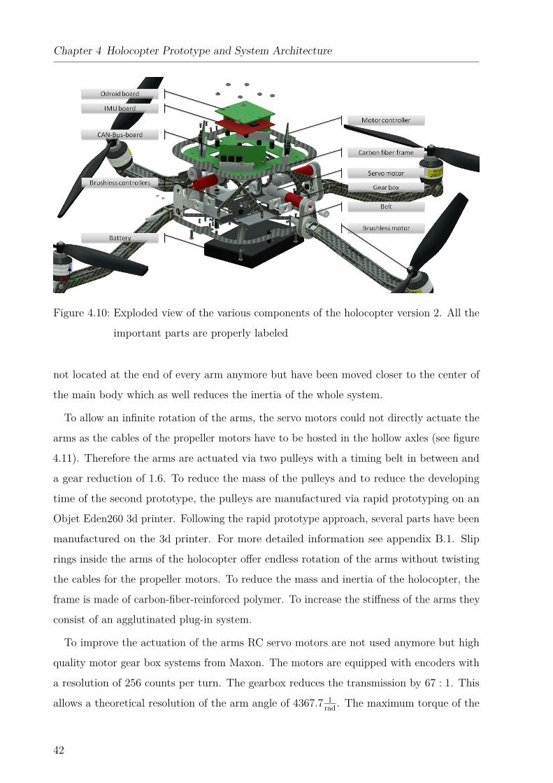
Chapter 4 Holocopter Prototype and System Architecture
Figure 4.10: Exploded view of the various components of the holocopter version 2. All the
important parts are properly labeled
not located at the end of every arm anymore but have been moved closer to the center of
the main body which as well reduces the inertia of the whole system.
To allow an infinite rotation of the arms, the servo motors could not directly actuate the
arms as the cables of the propeller motors have to be hosted in the hollow axles (see figure
4.11). Therefore the arms are actuated via two pulleys with a timing belt in between and
a gear reduction of 1.6. To reduce the mass of the pulleys and to reduce the developing
time of the second prototype, the pulleys are manufactured via rapid prototyping on an
Objet Eden260 3d printer. Following the rapid prototype approach, several parts have been
manufactured on the 3d printer. For more detailed information see appendix B.1. Slip
rings inside the arms of the holocopter offer endless rotation of the arms without twisting
the cables for the propeller motors. To reduce the mass and inertia of the holocopter, the
frame is made of carbon-fiber-reinforced polymer. To increase the stiffness of the arms they
consist of an agglutinated plug-in system.
To improve the actuation of the arms RC servo motors are not used anymore but high
quality motor gear box systems from Maxon. The motors are equipped with encoders with
a resolution of 256 counts per turn. The gearbox reduces the transmission by 67 : 1. This
allows a theoretical resolution of the arm angle of 4367.7 1rad . The maximum torque of the
42
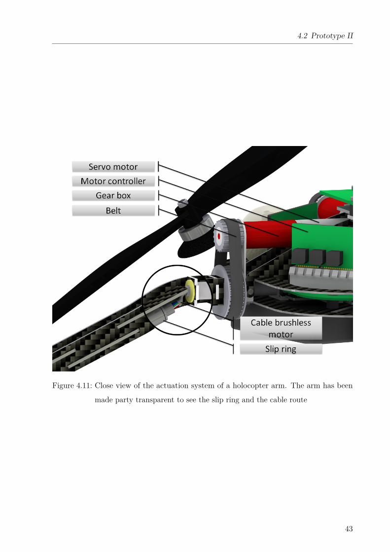
4.2 Prototype II
Figure 4.11: Close view of the actuation system of a holocopter arm. The arm has been
made party transparent to see the slip ring and the cable route
43
Chapter 4 Holocopter Prototype and System Architecture
whole actuation system including the transmission is τmax = 0.497 Nm and the maximum
velocity is α = 7.543 rads . The servo motors are driven by Maxon EPOS2 controllers.
The overall mass of the holocopter is m = 1.03 kg and from a high detail CAD model of
the body and propeller groups we also obtained the following inertia matrices
IPi=
7.15e−5 0 0
0 44.0e−5 0
0 0 41.3e−5
[kg m2
]
and
IB =
7.92e−4 0 0
0 9.99e−4 0
0 0 12.38e−4
[kg m2
].
The defined requirement for a reduction of the mass could be achieved with a nominal
reduction of 22%. If the inertia of the whole holocopter prototypes is compared (main
body including arms with α = 0 for all arms referred as IHC) a reduction of 20% has been
achieved for IHC11 and IHC22 while for IHC33 only a negligible reduction of 1% has been
achieved. This is due to a larger diameter of 52.5 mm of the second prototype and the fact
that an essential part of the mass is concentrated in the propeller motors that are on the
outer most of the diameter.
4.2.2 System architecture
The system architecture is similar to the first prototype but all parts have been updated to
later products. On board of the holocopter is a pico ATX format computer board equipped
with an Intel Atom D525, 1.83 GHz microprocessor and 4 GB DDR2 RAM. The OS running
on board is Ubuntu 12.04 LTS on a compact flash card.
EPOS2 controllers are high quality miniaturized position or velocity controllers for a
variety of motor types (e.g. brushed DC motors, brushless EC motors). They can either
be interfaced via CANopen or RS232. A single controller can be used as a gateway to
other EPOS controllers. As the computer module of the holocopter is not equipped with
a CAN-bus port the latter option has been implemented. A carrier board that has been
designed to host the 4 EPOS2 controllers is as well equipped with an USB to serial converter
(see appendix B.2). Following, the Intel Atom board is connected to the carrier board via
44
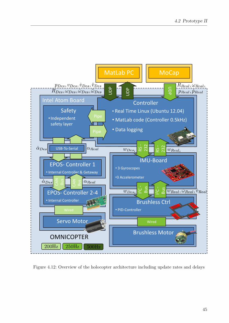
4.2 Prototype II
Intel Atom Board Controller
• Real Time Linux (Ubuntu 12.04)
• MatLab code (Controller 0.5kHz)
• Data logging
IMU-Board • 3 Gyroscopes
•3 Accelerometer
EPOS- Controller 2-4 • Internal Controller
Brushless Motor
Brushless Ctrl • PID-Controller
MatLab PC
Safety
• Independent safety layer
Servo Motor
Pipe
Pipe
RS
-2
32
RS
-2
32
I2C
-
Bu
s
I2C
-
Bu
s
Wired
Wired
OMNICOPTER
UD
P
UD
P
MoCap
UD
P
EPOS- Controller 1 • Internal Controller & Getaway
CA
NB
us
CA
N
Bu
s
USB-To-Serial
Figure 4.12: Overview of the holocopter architecture including update rates and delays
45
Chapter 4 Holocopter Prototype and System Architecture
USB. Here the bus data are converted to RS232-bus and send to the first EPOS controller.
The first EPOS controller is used as a gateway and connected to the three other EPOS
controllers via CAN-Bus (see figure 4.12).
The IMU-board and the brushless controllers are purchased from mikrokopter. Compared
to the first holocopter, IMU-board V2.1 (before V2.0) and brushless controller V2.0 (before
V1.2) are used now. The new brushless controllers allow for a higher thrust and a more
precise value resolution of the desired thrust of 11 bit (before 8 bit resolution). In the
new control scheme the desired servo arm position αDiand the current position αi is not
transmitted via the IMU board anymore therefore the overall traffic on the serial bus is
reduced. This allows for a general increase of the communication frequency of the desired
motor speed wi and the sensor reading frequency of the gyroscopes and accelerometers
(increased to 250 Hz).
The new holocopter is currently under final software development. Therefore all reported
flight experiments are performed with the first holocopter.
4.3 Energetic efficiency of the holocopter in hovering
As final consideration, we briefly discuss the energetic efficiency of the holocopter in a
hovering condition. Indeed, we note that the holocopter energetic efficiency for arbitrary
hovering orientations can be less than in the (standard) horizontal case (φ = 0, θ = 0), and
also despite the optimization action (3.14). This is due to the adopted mechanical design
which allows each propeller to ‘only’ rotate about one tilting angle (angles αi): therefore,
there will exist hovering orientations at which the thrust vectors T Picannot be aligned
against gravity, with thus some of the thrust lost in internal forces. This reduced efficiency
cannot be completely avoided with the adopted design, but only partially mitigated via
optimization actions such as (3.14). In this sense, the following Table 4.1 gives an illustration
of the energetic efficiency of our prototype (in terms of the mean spinning velocity of the
four propellers) obtained at several hovering conditions (including the horizontal one).
46
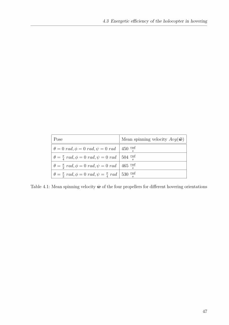
4.3 Energetic efficiency of the holocopter in hovering
Pose Mean spinning velocity Avg(w)
θ = 0 rad, φ = 0 rad, ψ = 0 rad 450 rads
θ = π4 rad, φ = 0 rad, ψ = 0 rad 504 rad
s
θ = π2 rad, φ = 0 rad, ψ = 0 rad 465 rad
s
θ = π2 rad, φ = 0 rad, ψ = π
4 rad 530 rads
Table 4.1: Mean spinning velocity w of the four propellers for different hovering orientations
47

Chapter 5
Simulation Results
This chapter has been mainly reproduced from an article published in IEEE Transactions
on Control Systems Technology: Ryll et al. (to be published 2014)
We now report simulation results aimed at validating the proposed control design. We
first consider in Sect. 5.1 an ‘ideal’ case in which controller (3.7) is tested on the complete
holocopter dynamical model of Sect. 2, that is, by including all the inertial and gyroscopic
effects neglected at the control design stage. These results are meant to illustrate the flying
performance of the holocopter in ideal conditions, that is, when not taking into account all
the limitations and non-idealities affecting the real prototype as in Sect. 4.1.3.
Subsequently, we present in Sect. 5.2 an additional set of ‘realistic’ simulations that
explicitly include the prototype main non-idealities (data exchange rates, control frequencies,
and actuation delays). In these simulations the controller (3.7) is also complemented with
the prediction scheme of Sect. 4.1.4 so as to replicate, as much as possible, the control
architecture of the real prototype. The results are intended to show the robustness of the
adopted control approach as the holocopter is still able to execute complex trajectories
although with a poorer flight performance compared to the ‘ideal’ case (as expected).
Furthermore, a comparison between both cases clearly shows the margin left for improving
the actuation system of our prototype in its second generation (see Sect. 8).
49
Chapter 5 Simulation Results
5.1 Ideal Simulations
The aim of the following simulations is twofold: on one side, we want to highlight the tracking
capabilities of the proposed controller and the beneficial action of the null-space term (19)
in avoiding singularities for the decoupling matrix A(α, ω). On the other side, we also want
to show the robustness of the controller against all the inertial/gyroscopic effects neglected
at the control design stage but included in the quadrotor dynamic model (2.1)–(2.4)–(2.5).
5.1.1 Rotation on spot
In this first simulation, we tested a simple trajectory involving a rotation of π rad on
the spot along the Y B axis1. The initial conditions were set to p(t0) = 0, p(t0) = 0,
R(t0) = I3, ωB(t0) = 0, α(t0) = 0, α(t0) = 0, and w(t0) = wrest. The desired trajectory
was chosen as pd(t) ≡ 0 and Rd(t) = RX(φ(t)) with φ(t) following a smooth profile with
maximum velocity φmax = 0.49 rad/s and maximum acceleration φmax = 0.16 rad/s2. The
trajectory was executed twice by (i) including and (ii) not including the null-space term
z (3.14) into (3.7) (kH = 1 or kH = 0). The gains in (3.9)–(3.11) were set to Kp1 = 28.5I3,
Kp2 = 271I3, Kp3 = 857I3 and Kω1 = 45 I3, Kω2 = 675 I3, and Kω3 = 3375I3.
Figures 5.2(a–f) show the results of the simulation in these two cases. In particular,
Fig. 5.2(a) shows the superimposition of H(w) when including z (red dashed line, case
(i)) and not including z (blue solid line, case (ii)). It is clear that, in the first case,
H(w) attains a lower value over time thanks to the optimization action in (3.14). As a
consequence, this results in a lower value for ‖w‖ over time as depicted in Fig. 5.2(b) (same
color pattern), showing that the given task (rotation on the spot) can be realized in a
more ‘energy-efficient’ way when properly shaping the cost function H(w). Note that, as
a byproduct, the better performance of case (i) comes at the expense of a more complex
reorientation of the propeller groups during the motion. This is shown in Figs. 5.2(c–d)
which report the behavior of the 4 tilt angles αi in cases (i) (left) and (ii) (right): compared
to Fig. 5.2(d), note the rotation of two propellers starting from t ≈ 25.8 [s] in Fig. 5.2(c).1This upside-down flip motion would be clearly unfeasible for a standard quadrotor. This trajectory is
a continuation of the illustrated trajectory in figure 4.2 where the first half rotation is shown. It is
(unfortunately) also unfeasible for the current experimental prototype because of the mechanical end
stops in the propeller tilting actuation, see Sect. 4.1.
50
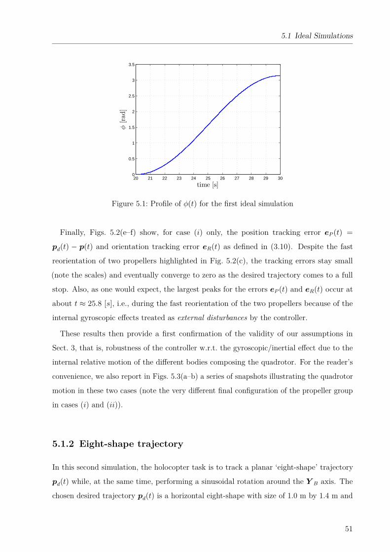
5.1 Ideal Simulations
20 21 22 23 24 25 26 27 28 29 300
0.5
1
1.5
2
2.5
3
3.5
φ[rad]
time [s]
Figure 5.1: Profile of φ(t) for the first ideal simulation
Finally, Figs. 5.2(e–f) show, for case (i) only, the position tracking error eP (t) =
pd(t) − p(t) and orientation tracking error eR(t) as defined in (3.10). Despite the fast
reorientation of two propellers highlighted in Fig. 5.2(c), the tracking errors stay small
(note the scales) and eventually converge to zero as the desired trajectory comes to a full
stop. Also, as one would expect, the largest peaks for the errors eP (t) and eR(t) occur at
about t ≈ 25.8 [s], i.e., during the fast reorientation of the two propellers because of the
internal gyroscopic effects treated as external disturbances by the controller.
These results then provide a first confirmation of the validity of our assumptions in
Sect. 3, that is, robustness of the controller w.r.t. the gyroscopic/inertial effect due to the
internal relative motion of the different bodies composing the quadrotor. For the reader’s
convenience, we also report in Figs. 5.3(a–b) a series of snapshots illustrating the quadrotor
motion in these two cases (note the very different final configuration of the propeller group
in cases (i) and (ii)).
5.1.2 Eight-shape trajectory
In this second simulation, the holocopter task is to track a planar ‘eight-shape’ trajectory
pd(t) while, at the same time, performing a sinusoidal rotation around the Y B axis. The
chosen desired trajectory pd(t) is a horizontal eight-shape with size of 1.0 m by 1.4 m and
51
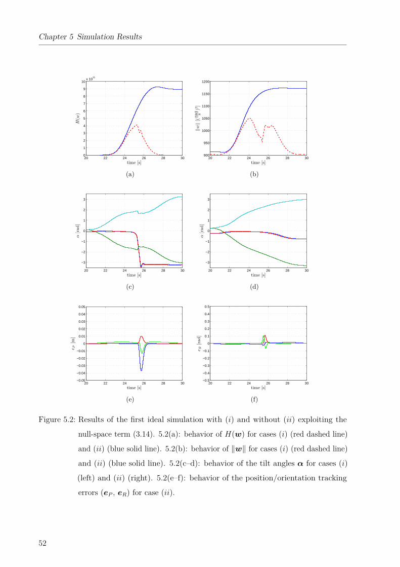
Chapter 5 Simulation Results
20 22 24 26 28 300
1
2
3
4
5
6
7
8
9
10x 10
11H(w
)
time [s]
(a)
20 22 24 26 28 30900
950
1000
1050
1100
1150
1200
||w||[(rad s)2]
time [s]
(b)
20 22 24 26 28 30
−3
−2
−1
0
1
2
3
α[rad]
time [s]
(c)
20 22 24 26 28 30
−3
−2
−1
0
1
2
3α[rad]
time [s]
(d)
20 22 24 26 28 30−0.05
−0.04
−0.03
−0.02
−0.01
0
0.01
0.02
0.03
0.04
0.05
eP[m
]
time [s]
(e)
20 22 24 26 28 30−0.5
−0.4
−0.3
−0.2
−0.1
0
0.1
0.2
0.3
0.4
0.5
eR[rad]
time [s]
(f)
Figure 5.2: Results of the first ideal simulation with (i) and without (ii) exploiting the
null-space term (3.14). 5.2(a): behavior of H(w) for cases (i) (red dashed line)
and (ii) (blue solid line). 5.2(b): behavior of ‖w‖ for cases (i) (red dashed line)
and (ii) (blue solid line). 5.2(c–d): behavior of the tilt angles α for cases (i)
(left) and (ii) (right). 5.2(e–f): behavior of the position/orientation tracking
errors (eP , eR) for case (ii).
52
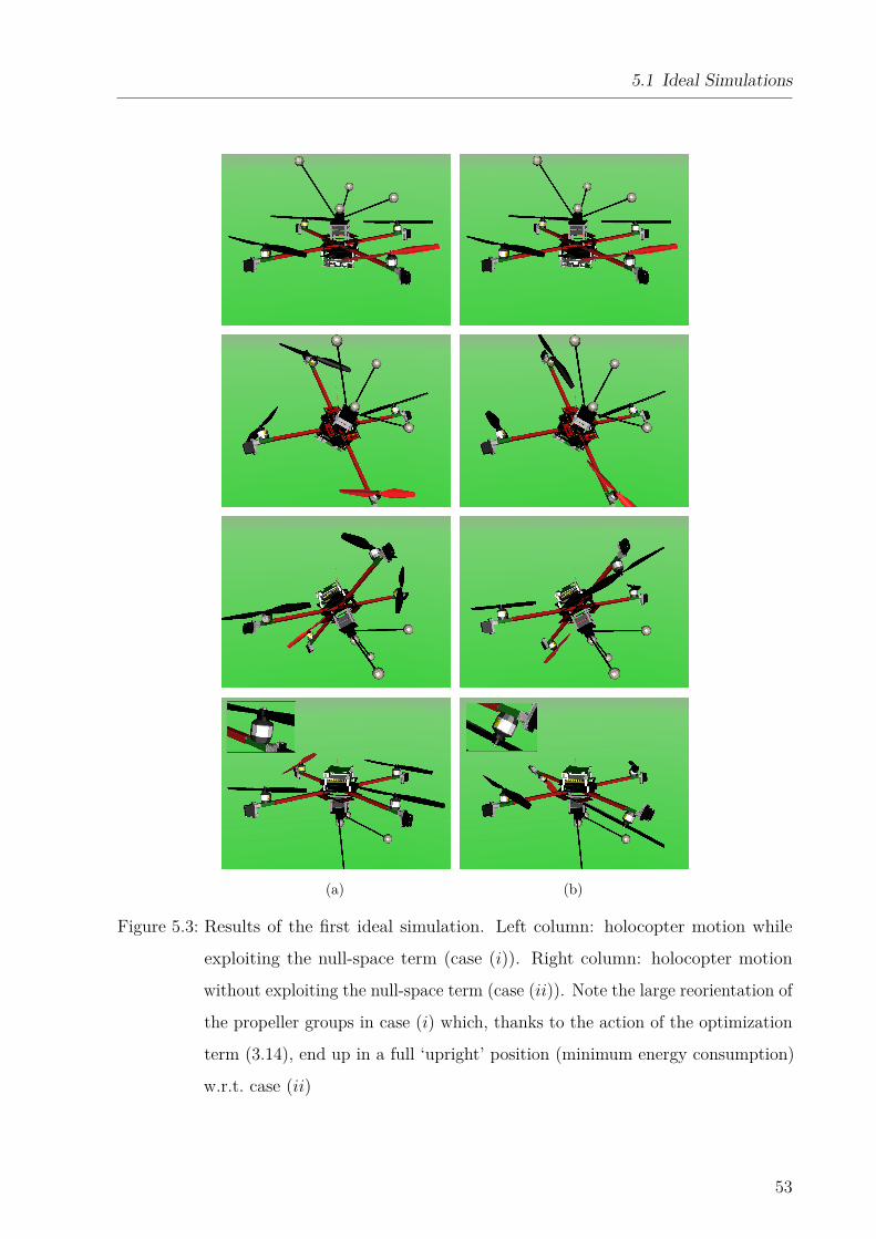
5.1 Ideal Simulations
(a) (b)
Figure 5.3: Results of the first ideal simulation. Left column: holocopter motion while
exploiting the null-space term (case (i)). Right column: holocopter motion
without exploiting the null-space term (case (ii)). Note the large reorientation of
the propeller groups in case (i) which, thanks to the action of the optimization
term (3.14), end up in a full ‘upright’ position (minimum energy consumption)
w.r.t. case (ii)
53
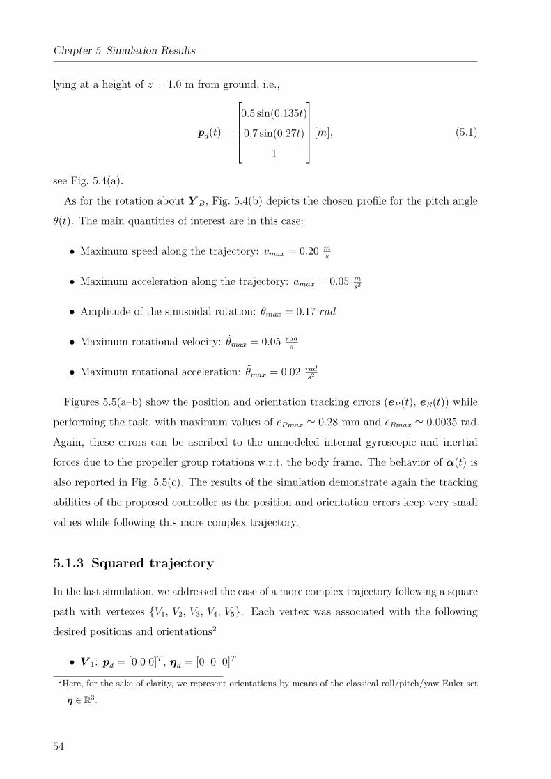
Chapter 5 Simulation Results
lying at a height of z = 1.0 m from ground, i.e.,
pd(t) =
0.5 sin(0.135t)
0.7 sin(0.27t)
1
[m], (5.1)
see Fig. 5.4(a).
As for the rotation about Y B, Fig. 5.4(b) depicts the chosen profile for the pitch angle
θ(t). The main quantities of interest are in this case:
• Maximum speed along the trajectory: vmax = 0.20 ms
• Maximum acceleration along the trajectory: amax = 0.05 ms2
• Amplitude of the sinusoidal rotation: θmax = 0.17 rad
• Maximum rotational velocity: θmax = 0.05 rads
• Maximum rotational acceleration: θmax = 0.02 rads2
Figures 5.5(a–b) show the position and orientation tracking errors (eP (t), eR(t)) while
performing the task, with maximum values of ePmax ' 0.28 mm and eRmax ' 0.0035 rad.
Again, these errors can be ascribed to the unmodeled internal gyroscopic and inertial
forces due to the propeller group rotations w.r.t. the body frame. The behavior of α(t) is
also reported in Fig. 5.5(c). The results of the simulation demonstrate again the tracking
abilities of the proposed controller as the position and orientation errors keep very small
values while following this more complex trajectory.
5.1.3 Squared trajectory
In the last simulation, we addressed the case of a more complex trajectory following a square
path with vertexes {V1, V2, V3, V4, V5}. Each vertex was associated with the following
desired positions and orientations2
• V 1: pd = [0 0 0]T , ηd = [0 0 0]T
2Here, for the sake of clarity, we represent orientations by means of the classical roll/pitch/yaw Euler set
η ∈ R3.
54
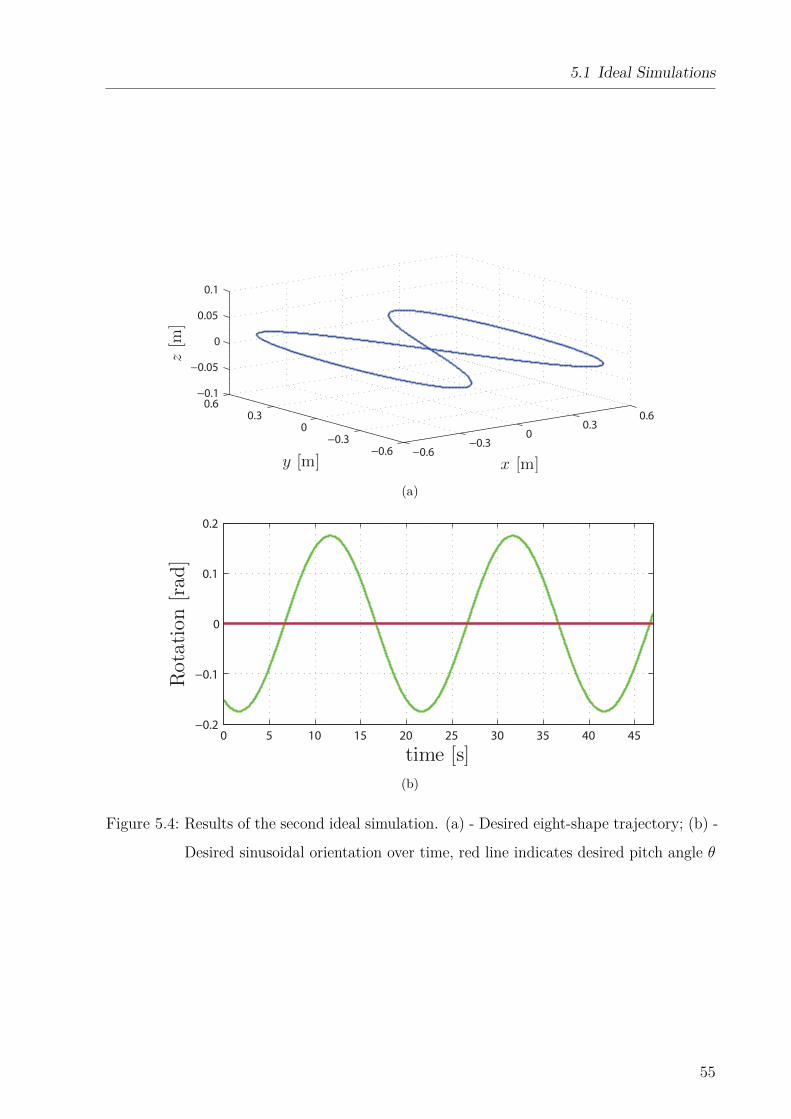
5.1 Ideal Simulations
−0.6−0.3
00.3
0.6
−0.6
−0.3
0
0.3
0.6−0.1
−0.05
0
0.05
0.1
x [m]y [m]
z[m
]
(a)
0 5 10 15 20 25 30 35 40 45−0.2
−0.1
0
0.1
0.2
Rotation[rad]
time [s]
(b)
Figure 5.4: Results of the second ideal simulation. (a) - Desired eight-shape trajectory; (b) -
Desired sinusoidal orientation over time, red line indicates desired pitch angle θ
55
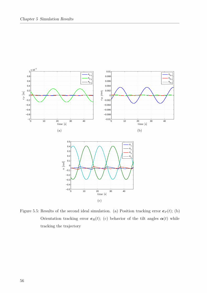
Chapter 5 Simulation Results
0 10 20 30 40−1
−0.8
−0.6
−0.4
−0.2
0
0.2
0.4
0.6
0.8
1x 10
−3
e P[m
]
time [s]
eP x
eP y
eP z
(a)
0 10 20 30 40−0.01
−0.008
−0.006
−0.004
−0.002
0
0.002
0.004
0.006
0.008
0.01
e R[rad]
time [s]
eR x
eR y
eR z
(b)
0 10 20 30 40−0.5
−0.4
−0.3
−0.2
−0.1
0
0.1
0.2
0.3
0.4
0.5
α[rad]
time [s]
α1
α2
α3
α4
(c)
Figure 5.5: Results of the second ideal simulation. (a) Position tracking error eP (t); (b)
Orientation tracking error eR(t); (c) behavior of the tilt angles α(t) while
tracking the trajectory
56
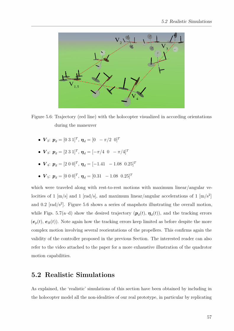
5.2 Realistic Simulations
Figure 5.6: Trajectory (red line) with the holocopter visualized in according orientations
during the maneuver
• V 2: pd = [0 3 1]T , ηd = [0 − π/2 0]T
• V 3: pd = [2 3 1]T , ηd = [−π/4 0 − π/4]T
• V 4: pd = [2 0 0]T , ηd = [−1.41 − 1.08 0.25]T
• V 5: pd = [0 0 0]T , ηd = [0.31 − 1.08 0.25]T
which were traveled along with rest-to-rest motions with maximum linear/angular ve-
locities of 1 [m/s] and 1 [rad/s], and maximum linear/angular accelerations of 1 [m/s2]
and 0.2 [rad/s2]. Figure 5.6 shows a series of snapshots illustrating the overall motion,
while Figs. 5.7(a–d) show the desired trajectory (pd(t), ηd(t)), and the tracking errors
(ep(t), eR(t)). Note again how the tracking errors keep limited as before despite the more
complex motion involving several reorientations of the propellers. This confirms again the
validity of the controller proposed in the previous Section. The interested reader can also
refer to the video attached to the paper for a more exhaustive illustration of the quadrotor
motion capabilities.
5.2 Realistic Simulations
As explained, the ‘realistic’ simulations of this section have been obtained by including in
the holocopter model all the non-idealities of our real prototype, in particular by replicating
57
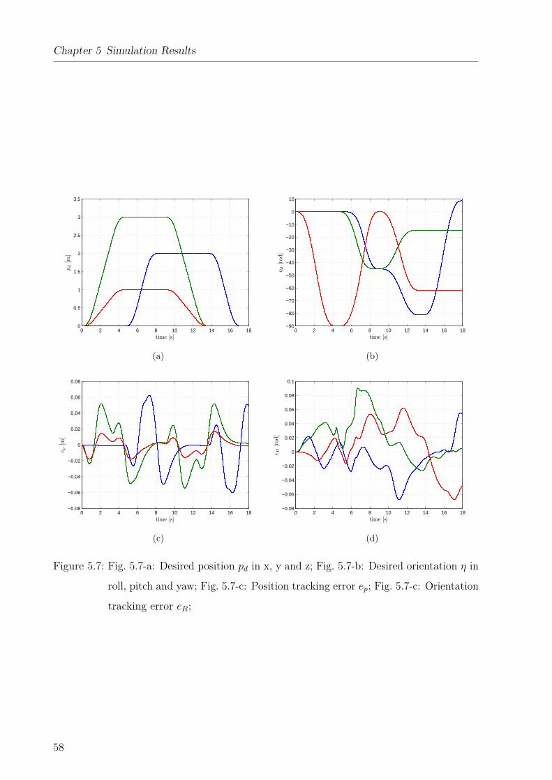
Chapter 5 Simulation Results
0 2 4 6 8 10 12 14 16 180
0.5
1
1.5
2
2.5
3
3.5
p d[m
]
time [s]
(a)
0 2 4 6 8 10 12 14 16 18−90
−80
−70
−60
−50
−40
−30
−20
−10
0
10
η d[rad
]
time [s]
(b)
0 2 4 6 8 10 12 14 16 18−0.08
−0.06
−0.04
−0.02
0
0.02
0.04
0.06
0.08
e p[m
]
time [s]
(c)
0 2 4 6 8 10 12 14 16 18−0.08
−0.06
−0.04
−0.02
0
0.02
0.04
0.06
0.08
0.1
e R[rad]
time [s]
(d)
Figure 5.7: Fig. 5.7-a: Desired position pd in x, y and z; Fig. 5.7-b: Desired orientation η in
roll, pitch and yaw; Fig. 5.7-c: Position tracking error ep; Fig. 5.7-c: Orientation
tracking error eR;
58
5.2 Realistic Simulations
the various signal and control frequencies (e.g., motion capture frequency at 200 Hz, servo
motor frequency at 70 Hz) and delays (e.g., servo motor delay of 18 ms). In addition,
we also considered the noise of onboard sensor readings (gyroscopes, accelerometers and
measurement of angles α), of the actuators (servo and propeller motors), and of the
motion capture system by either obtaining the noise characteristics from data sheets, or
via a preliminary off-line identification. Finally, the prediction scheme of Sect. 4.1.4 was
implemented in the control loop.
To identify the noise level of the used motion capture system two experiments have been
conducted. In the first experiment the position and orientation of a static object has been
measured over time while in the second experiment the object was in motion. The standard
variation of the position and orientation has been calculated in both cases. For the static
case the noise has been found as being negligible with a standard deviation of
V (pstatic) =
2.7472e−10
5.1316e−10
2.3642e−10
[m2], V (Rstatic) =
1.6769e−08
1.7920e−08
1.5669e−08
[rad2]. (5.2)
For the dynamic case the standard deviation has been found as
V (pdynamic) =
4.5375e−4
4.4425e−4
2.2471e−7
[m2], V (Rdynamic) =
7.7348e−7
8.1188e−7
1.0425e−4
[rad2]. (5.3)
Here the error is not negligible anymore. The simulated MoCap position and orientation
data have thus been modeled with a standard deviation according to the values obtained
from the lalter case.
Despite assessing the effects of these non-idealities on the overall flight performance, the
results of this section are also helpful for saving development time as they allow a pre-tuning
of the various control gains for the deployment on the real prototype, and the identification
of the most influential parameters to be optimized in view of a second-generation prototype.
5.2.1 Rotation on Spot
Because of the limited range of the tilting angles α in the real prototype, it is not possible
to perform a full rotation on the spot as in the previous ideal case of Sect. 5.1.1. Therefore
59
Chapter 5 Simulation Results
we opted for a (more feasible) sinusoidal rotation around the Y B-axis (pitch), i.e., with
Rd(t) = RY (θ(t)) with θmax = 0.436 rad and θmax = 0.07 rad/s. The initial conditions
were set to hovering (p(t0) = 0, p(t0) = 0, R(t0) = I3, ωB(t0) = 0, α(t0) = 0, and
w(t0) = wrest), and the controller gains were chosen as Kp1 = 30I3, Kω1 = 55.5I3,
Kp2 = 300I3, Kω2 = 1027I3, Kp3 = 1000I3, Kω3 = 6331I3.
The results are reported in Fig. 5.8(a–d): Fig. 5.8(a) shows the behavior of the quadrotor
orientation during flight (blue - roll, green - pitch, red - yaw) and Fig. 5.8(b) the behavior
of the orientation error eR(t). The maximum rotation errors are 0.240 rad (roll), 0.079 rad
(pitch), and 0.144 rad (yaw). Figure 5.8(c) shows the behavior of the position tracking
error eP (t) characterized by a mean value avg(‖eP (t)‖) ≈ 1.6 cm and a maximum value
max(‖eP (t)‖) ≈ 4.4 cm. Finally, Figure 5.8(d) shows the behavior of the tilting angles α(t)
over time.
Therefore, despite the (expected) worse overall performance w.r.t. the ‘ideal’ case, in this
‘realistic’ case the holocopter is still able to fulfill the assigned motion task with a good
enough accuracy.
5.2.2 Eight-shape trajectory
In this simulation we considered the same eight-shape trajectory of Sect. 5.1.2. Figures 5.9(a–
b) report the behavior of the position and orientation error vectors (eP (t), eR(t)) over
time. The average position tracking error results about 0.034 m with a maximum of
0.050 m. The maximum rotation errors are 0.097 rad (roll), 0.061 rad (pitch), and 0.039 rad
(yaw). Finally, Fig. 5.9(c) shows the behavior of the tilting angles αi(t) while following the
trajectory.
It is interesting to compare these results with those of the ‘ideal’ simulation of Sect. 5.1.2
(Figs. 5.5(a–c)): again, the overall tracking performance results degraded w.r.t. the ideal
case, although the holocopter can still realize the task with a sufficient accuracy. Also, note
how the angles αi(t) in Fig. 5.9(c) follow essentially the same behavior as those of the ideal
case in Fig. 5.5(c) despite the higher noise level present in the system.
60
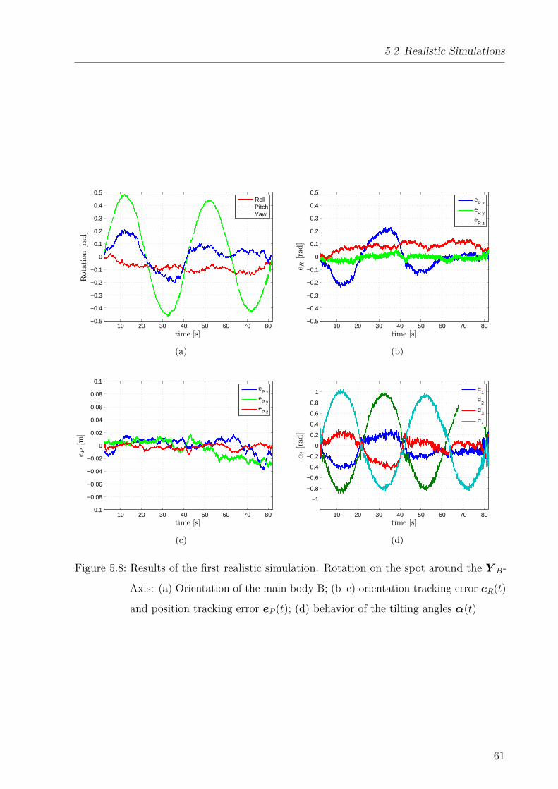
5.2 Realistic Simulations
10 20 30 40 50 60 70 80−0.5
−0.4
−0.3
−0.2
−0.1
0
0.1
0.2
0.3
0.4
0.5
Rotation[rad]
time [s]
RollPitchYaw
(a)
10 20 30 40 50 60 70 80−0.5
−0.4
−0.3
−0.2
−0.1
0
0.1
0.2
0.3
0.4
0.5
e R[rad]
time [s]
eR x
eR y
eR z
(b)
10 20 30 40 50 60 70 80−0.1
−0.08
−0.06
−0.04
−0.02
0
0.02
0.04
0.06
0.08
0.1
e P[m
]
time [s]
eP x
eP y
eP z
(c)
10 20 30 40 50 60 70 80
−1
−0.8
−0.6
−0.4
−0.2
0
0.2
0.4
0.6
0.8
1
αi[rad]
time [s]
α1
α2
α3
α4
(d)
Figure 5.8: Results of the first realistic simulation. Rotation on the spot around the Y B-
Axis: (a) Orientation of the main body B; (b–c) orientation tracking error eR(t)
and position tracking error eP (t); (d) behavior of the tilting angles α(t)
61
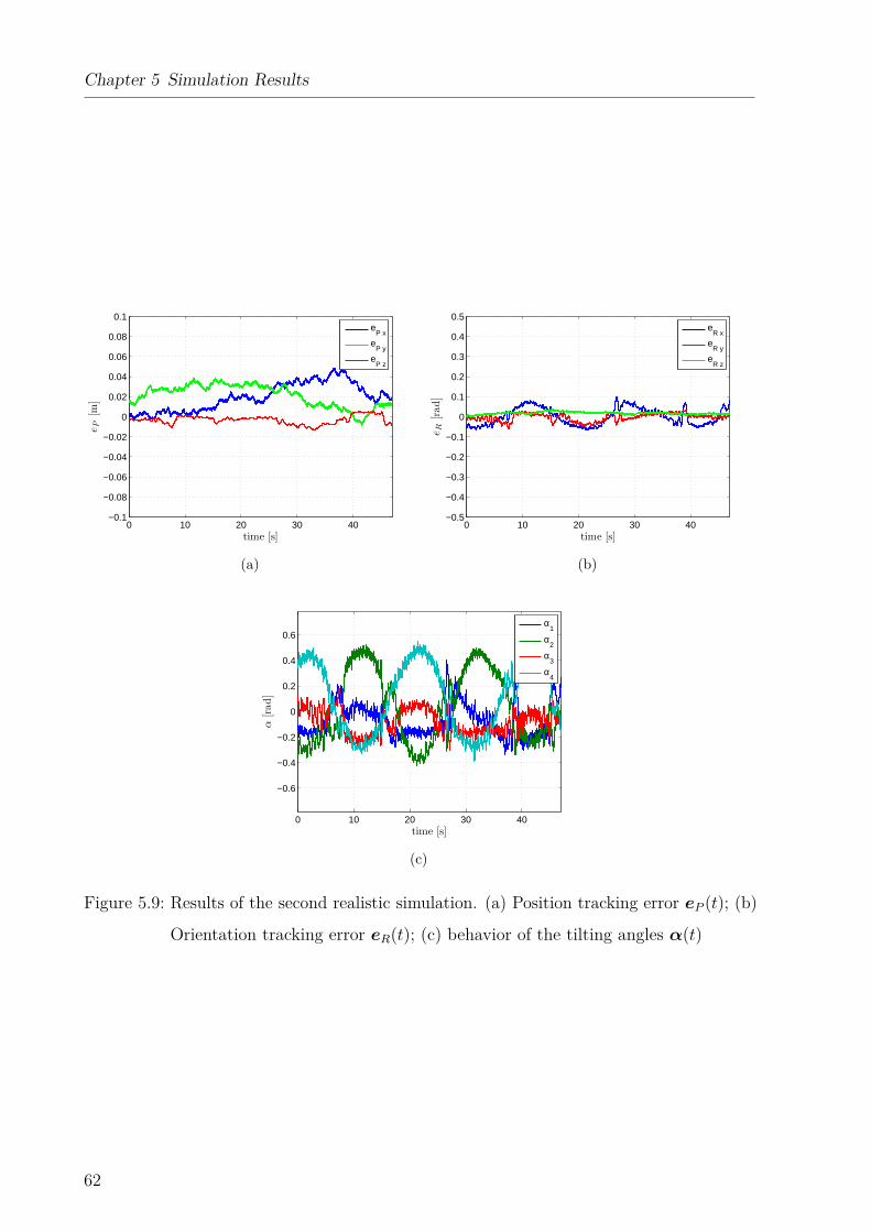
Chapter 5 Simulation Results
0 10 20 30 40−0.1
−0.08
−0.06
−0.04
−0.02
0
0.02
0.04
0.06
0.08
0.1
e P[m
]
time [s]
eP x
eP y
eP z
(a)
0 10 20 30 40−0.5
−0.4
−0.3
−0.2
−0.1
0
0.1
0.2
0.3
0.4
0.5
e R[rad]
time [s]
eR x
eR y
eR z
(b)
0 10 20 30 40
−0.6
−0.4
−0.2
0
0.2
0.4
0.6
α[rad]
time [s]
α1
α2
α3
α4
(c)
Figure 5.9: Results of the second realistic simulation. (a) Position tracking error eP (t); (b)
Orientation tracking error eR(t); (c) behavior of the tilting angles α(t)
62
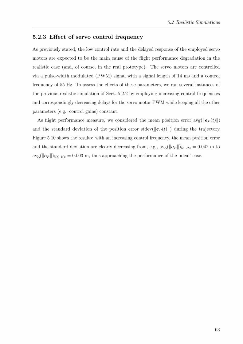
5.2 Realistic Simulations
5.2.3 Effect of servo control frequency
As previously stated, the low control rate and the delayed response of the employed servo
motors are expected to be the main cause of the flight performance degradation in the
realistic case (and, of course, in the real prototype). The servo motors are controlled
via a pulse-width modulated (PWM) signal with a signal length of 14 ms and a control
frequency of 55 Hz. To assess the effects of these parameters, we ran several instances of
the previous realistic simulation of Sect. 5.2.2 by employing increasing control frequencies
and correspondingly decreasing delays for the servo motor PWM while keeping all the other
parameters (e.g., control gains) constant.
As flight performance measure, we considered the mean position error avg(‖eP (t)‖)
and the standard deviation of the position error stdev(‖eP (t)‖) during the trajectory.
Figure 5.10 shows the results: with an increasing control frequency, the mean position error
and the standard deviation are clearly decreasing from, e.g., avg(‖eP‖)55 Hz = 0.042 m to
avg(‖eP‖)500 Hz = 0.003 m, thus approaching the performance of the ‘ideal’ case.
63
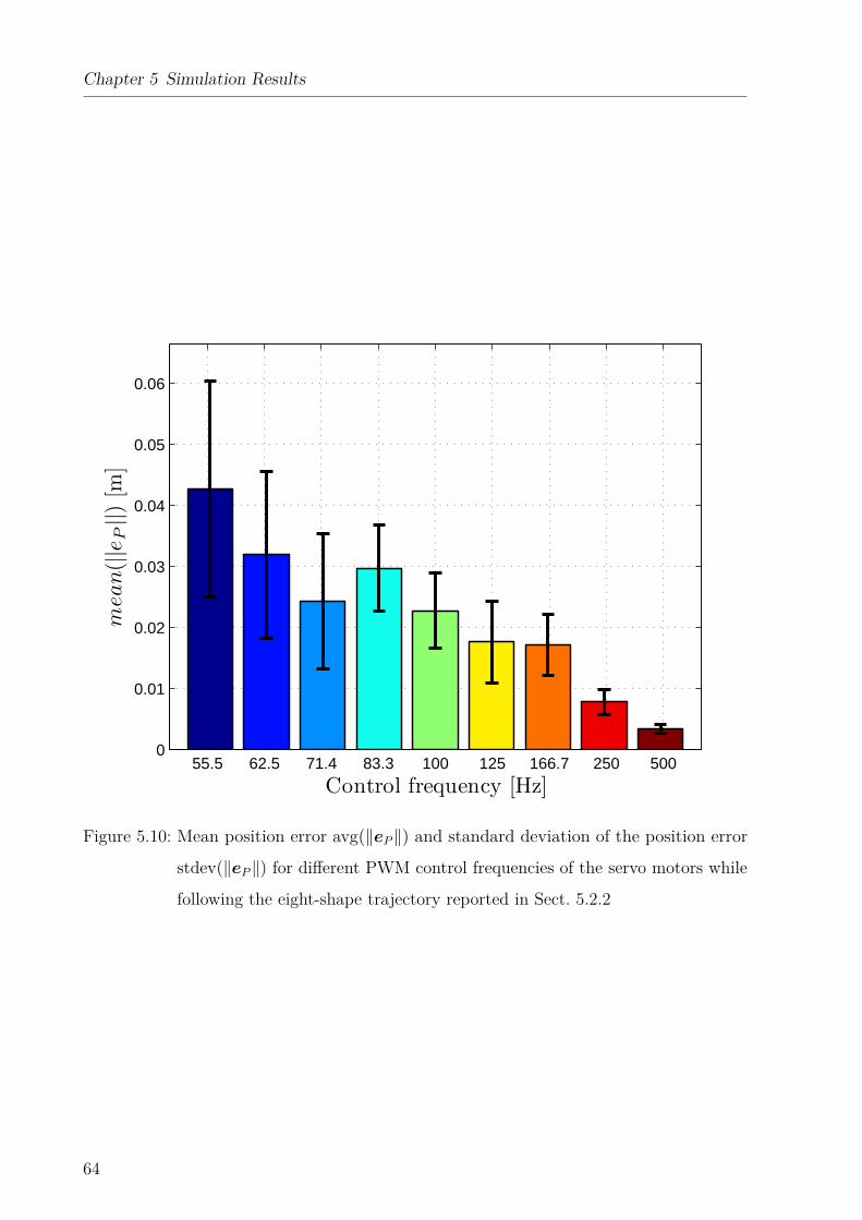
Chapter 5 Simulation Results
55.5 62.5 71.4 83.3 100 125 166.7 250 5000
0.01
0.02
0.03
0.04
0.05
0.06
mea
n(||e P
||)[m
]
Control frequency [Hz]
Figure 5.10: Mean position error avg(‖eP‖) and standard deviation of the position error
stdev(‖eP‖) for different PWM control frequencies of the servo motors while
following the eight-shape trajectory reported in Sect. 5.2.2
64
Chapter 6
Experimental Results
This chapter has been mainly reproduced from an article published in IEEE Transactions
on Control Systems Technology: Ryll et al. (to be published 2014)
In this last section we finally present results from three experiments conducted with the
holocopter prototype. The first experiment is a hovering task meant to show the overall
performance in the simplest scenario, and also to highlight again the importance of having
included the null-space optimization term (3.14) in the control strategy. The other two
experiments involve instead the more complex trajectories of Sect. 5.2.1 and Sect. 5.2.2.
Finally we encourage the reader to watch the video clip available at http://youtu.be/
hA-uNHW8MLE where several holocopter maneuvers are shown along with additional details
on the employed prototype.
6.1 Hovering on the spot
In the first experiment, following what was done in the ‘ideal’ case of Sect. 5.1.1, we show
the importance of having included the minimization of the cost function H(w) in the
proposed controller. To this end, we report the results of a simple hovering on the spot by
(i) including and (ii) not including the null-space optimization term (3.14).
The quadrotor starts from the initial state of p(t0) = 0, p(t0) = 0, R(t0) = I3, ωB(t0) =
0, α(t0) = 0, and w(t0) = wrest, and is commanded to stay still while maintaining
the desired attitude Rd = I3. The gains in (3.9) and (3.11) were set to Kp1 = 30I3,
Kω1 = 55.5I3, Kp2 = 300I3, Kω2 = 1027I3, Kp3 = 1000I3, Kω3 = 6331I3 (these values
65
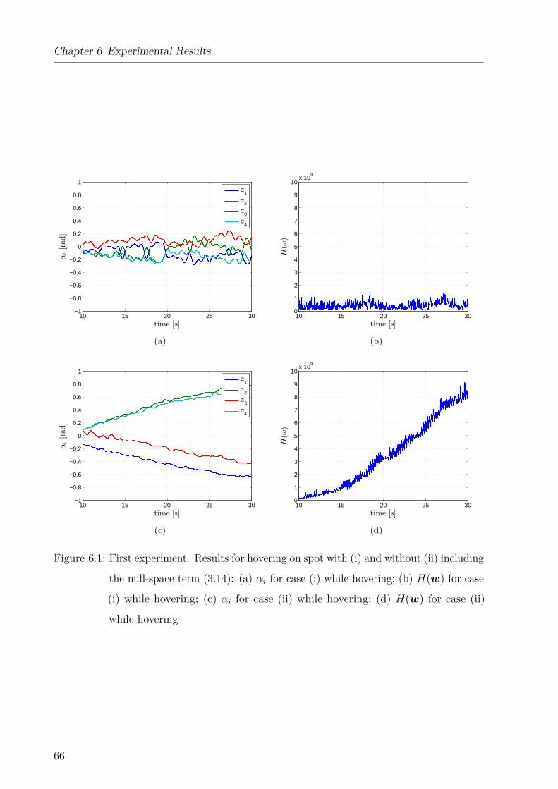
Chapter 6 Experimental Results
10 15 20 25 30−1
−0.8
−0.6
−0.4
−0.2
0
0.2
0.4
0.6
0.8
1
αi[rad]
time [s]
α1
α2
α3
α4
(a)
10 15 20 25 300
1
2
3
4
5
6
7
8
9
10x 10
9
H(ω
)
time [s]
(b)
10 15 20 25 30−1
−0.8
−0.6
−0.4
−0.2
0
0.2
0.4
0.6
0.8
1
αi[rad]
time [s]
α1
α2
α3
α4
(c)
10 15 20 25 300
1
2
3
4
5
6
7
8
9
10x 10
9
H(ω
)
time [s]
(d)
Figure 6.1: First experiment. Results for hovering on spot with (i) and without (ii) including
the null-space term (3.14): (a) αi for case (i) while hovering; (b) H(w) for case
(i) while hovering; (c) αi for case (ii) while hovering; (d) H(w) for case (ii)
while hovering
66
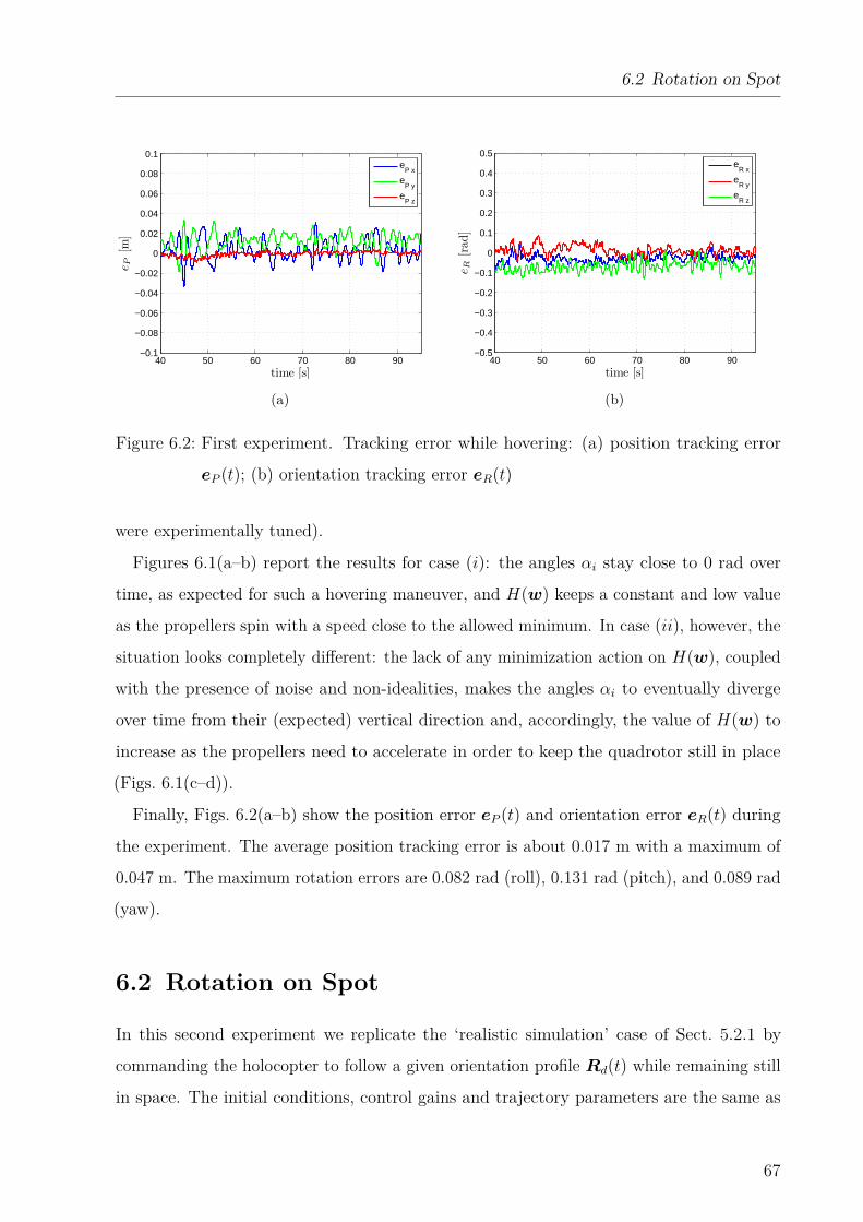
6.2 Rotation on Spot
40 50 60 70 80 90−0.1
−0.08
−0.06
−0.04
−0.02
0
0.02
0.04
0.06
0.08
0.1
e P[m
]
time [s]
eP x
eP y
eP z
(a)
40 50 60 70 80 90−0.5
−0.4
−0.3
−0.2
−0.1
0
0.1
0.2
0.3
0.4
0.5
e R[rad]
time [s]
eR x
eR y
eR z
(b)
Figure 6.2: First experiment. Tracking error while hovering: (a) position tracking error
eP (t); (b) orientation tracking error eR(t)
were experimentally tuned).
Figures 6.1(a–b) report the results for case (i): the angles αi stay close to 0 rad over
time, as expected for such a hovering maneuver, and H(w) keeps a constant and low value
as the propellers spin with a speed close to the allowed minimum. In case (ii), however, the
situation looks completely different: the lack of any minimization action on H(w), coupled
with the presence of noise and non-idealities, makes the angles αi to eventually diverge
over time from their (expected) vertical direction and, accordingly, the value of H(w) to
increase as the propellers need to accelerate in order to keep the quadrotor still in place
(Figs. 6.1(c–d)).
Finally, Figs. 6.2(a–b) show the position error eP (t) and orientation error eR(t) during
the experiment. The average position tracking error is about 0.017 m with a maximum of
0.047 m. The maximum rotation errors are 0.082 rad (roll), 0.131 rad (pitch), and 0.089 rad
(yaw).
6.2 Rotation on Spot
In this second experiment we replicate the ‘realistic simulation’ case of Sect. 5.2.1 by
commanding the holocopter to follow a given orientation profile Rd(t) while remaining still
in space. The initial conditions, control gains and trajectory parameters are the same as
67
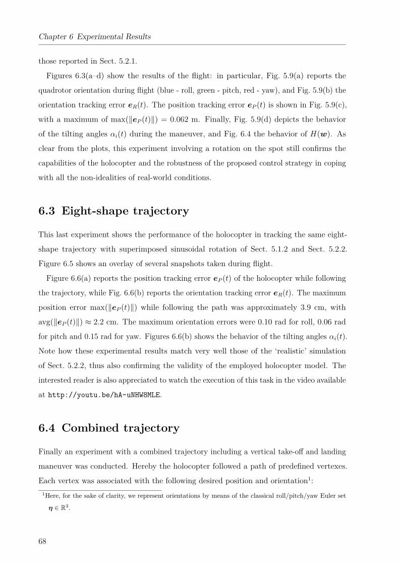
Chapter 6 Experimental Results
those reported in Sect. 5.2.1.
Figures 6.3(a–d) show the results of the flight: in particular, Fig. 5.9(a) reports the
quadrotor orientation during flight (blue - roll, green - pitch, red - yaw), and Fig. 5.9(b) the
orientation tracking error eR(t). The position tracking error eP (t) is shown in Fig. 5.9(c),
with a maximum of max(‖eP (t)‖) = 0.062 m. Finally, Fig. 5.9(d) depicts the behavior
of the tilting angles αi(t) during the maneuver, and Fig. 6.4 the behavior of H(w). As
clear from the plots, this experiment involving a rotation on the spot still confirms the
capabilities of the holocopter and the robustness of the proposed control strategy in coping
with all the non-idealities of real-world conditions.
6.3 Eight-shape trajectory
This last experiment shows the performance of the holocopter in tracking the same eight-
shape trajectory with superimposed sinusoidal rotation of Sect. 5.1.2 and Sect. 5.2.2.
Figure 6.5 shows an overlay of several snapshots taken during flight.
Figure 6.6(a) reports the position tracking error eP (t) of the holocopter while following
the trajectory, while Fig. 6.6(b) reports the orientation tracking error eR(t). The maximum
position error max(‖eP (t)‖) while following the path was approximately 3.9 cm, with
avg(‖eP (t)‖) ≈ 2.2 cm. The maximum orientation errors were 0.10 rad for roll, 0.06 rad
for pitch and 0.15 rad for yaw. Figures 6.6(b) shows the behavior of the tilting angles αi(t).
Note how these experimental results match very well those of the ‘realistic’ simulation
of Sect. 5.2.2, thus also confirming the validity of the employed holocopter model. The
interested reader is also appreciated to watch the execution of this task in the video available
at http://youtu.be/hA-uNHW8MLE.
6.4 Combined trajectory
Finally an experiment with a combined trajectory including a vertical take-off and landing
maneuver was conducted. Hereby the holocopter followed a path of predefined vertexes.
Each vertex was associated with the following desired position and orientation1:1Here, for the sake of clarity, we represent orientations by means of the classical roll/pitch/yaw Euler set
η ∈ R3.
68
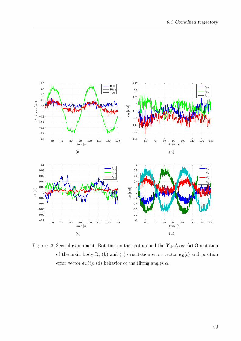
6.4 Combined trajectory
60 70 80 90 100 110 120 130−0.5
−0.4
−0.3
−0.2
−0.1
0
0.1
0.2
0.3
0.4
0.5
Rotation[rad]
time [s]
RollPitchYaw
(a)
60 70 80 90 100 110 120 130−0.25
−0.2
−0.15
−0.1
−0.05
0
0.05
0.1
0.15
e R[rad]
time [s]
eR x
eR y
eR z
(b)
60 70 80 90 100 110 120 130−0.1
−0.08
−0.06
−0.04
−0.02
0
0.02
0.04
0.06
0.08
0.1
e P[m
]
time [s]
eP x
eP y
eP z
(c)
60 70 80 90 100 110 120 130−1
−0.8
−0.6
−0.4
−0.2
0
0.2
0.4
0.6
0.8
1
αi[rad]
time [s]
α1
α2
α3
α4
(d)
Figure 6.3: Second experiment. Rotation on the spot around the Y B-Axis: (a) Orientation
of the main body B; (b) and (c) orientation error vector eR(t) and position
error vector eP (t); (d) behavior of the tilting angles αi
69
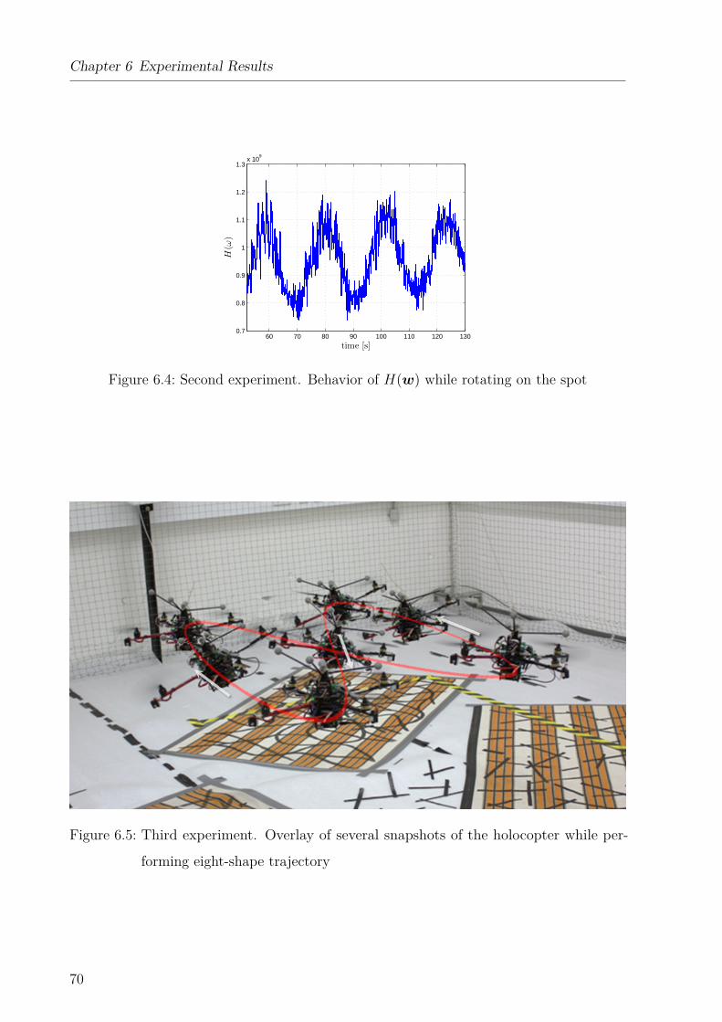
Chapter 6 Experimental Results
60 70 80 90 100 110 120 1300.7
0.8
0.9
1
1.1
1.2
1.3x 10
9
H(ω
)
time [s]
Figure 6.4: Second experiment. Behavior of H(w) while rotating on the spot
Figure 6.5: Third experiment. Overlay of several snapshots of the holocopter while per-
forming eight-shape trajectory
70
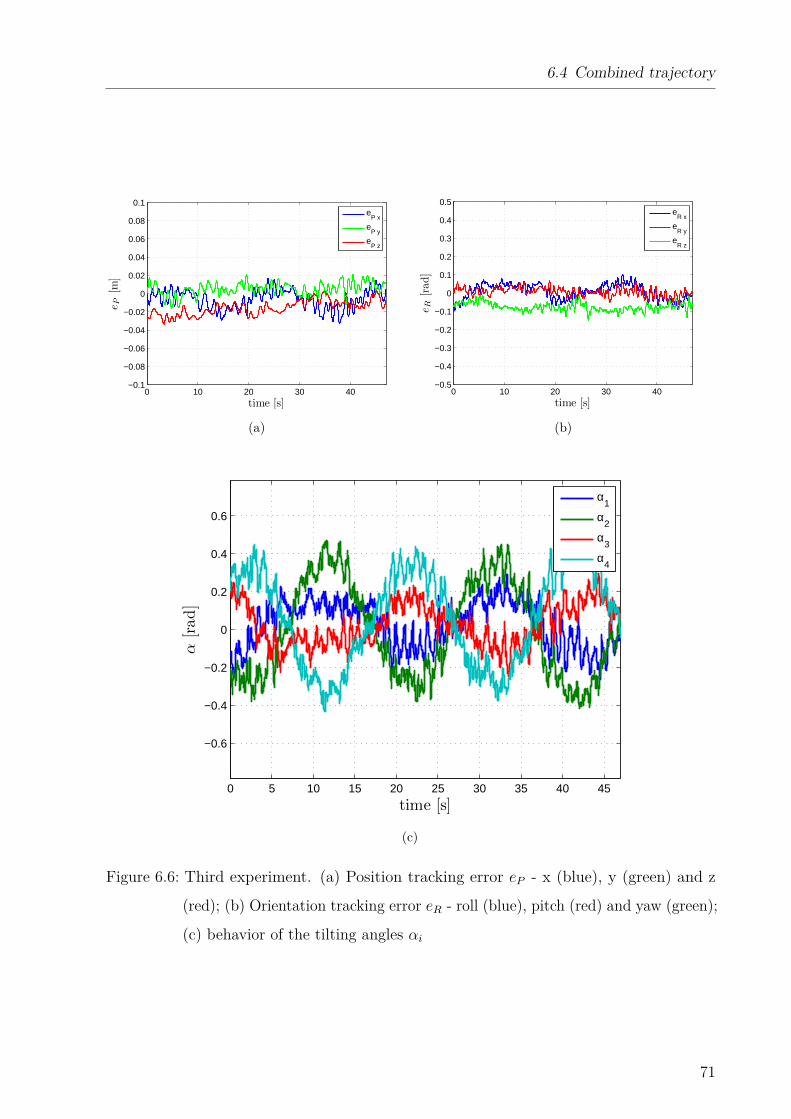
6.4 Combined trajectory
0 10 20 30 40−0.1
−0.08
−0.06
−0.04
−0.02
0
0.02
0.04
0.06
0.08
0.1
e P[m
]
time [s]
eP x
eP y
eP z
(a)
0 10 20 30 40−0.5
−0.4
−0.3
−0.2
−0.1
0
0.1
0.2
0.3
0.4
0.5
e R[rad]
time [s]
eR x
eR y
eR z
(b)
0 5 10 15 20 25 30 35 40 45
−0.6
−0.4
−0.2
0
0.2
0.4
0.6
α[rad]
time [s]
α
1
α2
α3
α4
(c)
Figure 6.6: Third experiment. (a) Position tracking error eP - x (blue), y (green) and z
(red); (b) Orientation tracking error eR - roll (blue), pitch (red) and yaw (green);
(c) behavior of the tilting angles αi
71

Chapter 6 Experimental Results
• V 1: pd = [0.33 − 0.17 0.7]T , ηd = [0 0 0]T
• V 2: pd = [0.33 − 0.17 1.0]T , ηd = [0 0 0]T
• V 3: pd = [0.0 0.0 1.05]T , ηd = [0 0 0]T
• V 4: pd = [0.0 0.0 1.05]T , ηd = [ π12 0 0]T
• V 5: pd = [0.0 0.0 1.05]T , ηd = [ π12 0 2π]T
• V 6: pd = [0.0 0.0 1.05]T , ηd = [0 0 2π]T
• V 7: pd = [0.33 − 0.17 1.15]T , ηd = [0 0 2π]T
• V 8: pd = [0.33 − 0.17 0.7]T , ηd = [0 0 2π]T
The performed trajectory is plotted in figure 6.7-(a) and (b). The take-off and landing
platform was located at the position pd = [0.33 − 0.17 0.8]T . The actually desired
landing and starting positions V1 and V8 could therefore not be achieved. The mismatch
between desired and actual landing position was consciously chosen to achieve a more
stable behavior in the lift-off and touch-down moment. The maximum translational
velocity is ||pBmax|| = 0.21 m
s and the maximum rotational velocity during the trajectory is
||ωBmax|| = 0.26 rads .
The maximum position error max(‖eP (t)‖) while following the path was approximately
9.8 cm, with avg(‖eP (t)‖) ≈ 3.7 cm. The maximum orientation errors were 0.10 rad for roll,
0.25 rad for pitch and 0.07 rad for yaw. Figure 6.7-(d) shows the advanced and continuous
reorientation of the servo motors.
6.5 Summary
In this section we presented a broad variety of experimental results starting from ’Hovering
on Spot’-maneuvers where the benefit and importance of the optimization from Section 3.2
over simple trajectories (see Sect. 6.2) although impossible for common quadrotors to finally
more advanced trajectories with multiple overlaid transitions and rotation including take-off
and landing in Section 6.4. We showed that the presented controller from Section 3 is able
to control the holocopter main body independently in position and orientation as originally
72
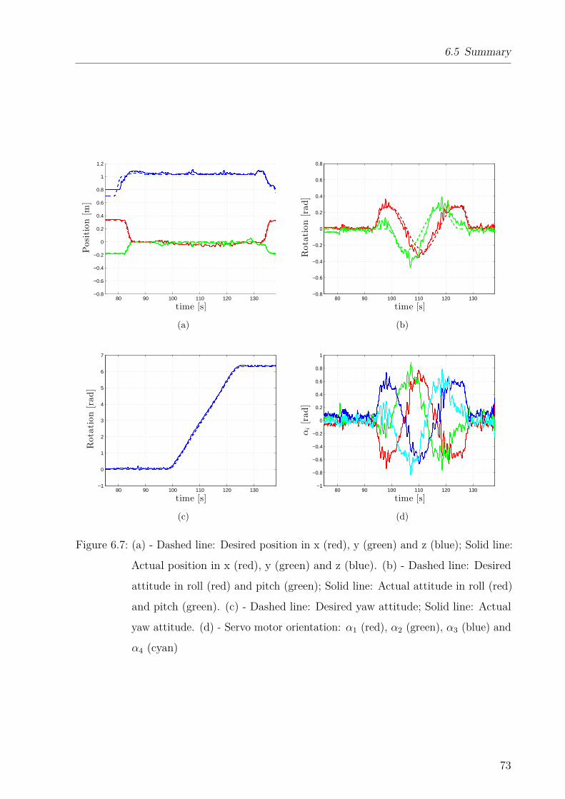
6.5 Summary
80 90 100 110 120 130−0.8
−0.6
−0.4
−0.2
0
0.2
0.4
0.6
0.8
1
1.2
Position[m
]
time [s]
(a)
80 90 100 110 120 130−0.8
−0.6
−0.4
−0.2
0
0.2
0.4
0.6
0.8
Rotation[rad]
time [s]
(b)
80 90 100 110 120 130−1
0
1
2
3
4
5
6
7
Rotation[rad]
time [s]
(c)
80 90 100 110 120 130−1
−0.8
−0.6
−0.4
−0.2
0
0.2
0.4
0.6
0.8
1
αi[rad]
time [s]
(d)
Figure 6.7: (a) - Dashed line: Desired position in x (red), y (green) and z (blue); Solid line:
Actual position in x (red), y (green) and z (blue). (b) - Dashed line: Desired
attitude in roll (red) and pitch (green); Solid line: Actual attitude in roll (red)
and pitch (green). (c) - Dashed line: Desired yaw attitude; Solid line: Actual
yaw attitude. (d) - Servo motor orientation: α1 (red), α2 (green), α3 (blue) and
α4 (cyan)
73
Chapter 6 Experimental Results
proposed. With this section the experimental results end and we will now present an outline
on possible interaction control scenarios with the holocopter.
74
Chapter 7
Perspectives on Aerial Interaction
Aerial manipulation of the environment and cooperative interaction with other robots
(UAVs or ground robots) is an emerging field of research. In cooperative arrangements,
UAVs are used to collectively transport higher payloads (e.g. Fink et al. (2010)) or to
manipulate a single airborne object (e.g. Michael et al. (2009) and Sreenath and Kumar
(2013)). Different approaches aim to use a single UAV to interact with the environment
either for inspection scenarios where a constant force has to be applied to an object (see
Forte et al. (2012a)) or more general a single UAV can also be used to apply arbitrary
forces on an object (see Gioioso et al. (2013)). A general drawback of standard UAVs
for manipulation is their intrinsic underactuation which results in a limited interaction
with the environment. As in the aforementioned publications several UAVs are needed to
manipulate an object or only a subset of possible forces and torques can be applied on an
object. This limitation does not hold for the holocopter where one clearly benefits from
the full actuation of the main body B. This final chapter will provide some guidelines
for possible future applications involving the interaction between the holocopter and the
physical world.
To get an insight on the importance of a well designed control scheme for interaction
tasks, one can note that tracking a desired end-effector trajectory will always imply presence
of some tracking errors (especially in the context of aerial manipulation). In an interaction
task this may result in a contact force and an additional deviation of the end effector
position. A standard control scheme will try to generate forces which attempt to reduce
the tracking error, and this will additionally increase the contact forces. A high stiffness
75
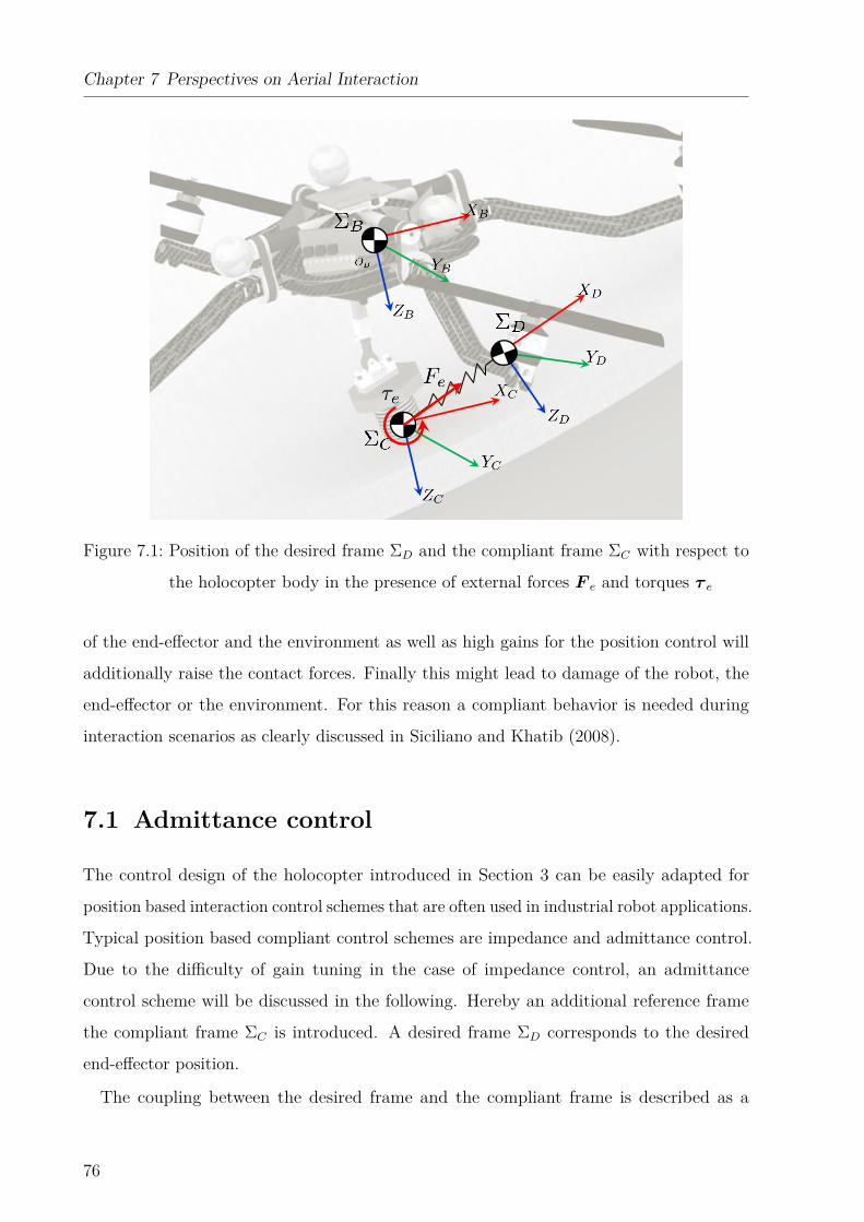
Chapter 7 Perspectives on Aerial Interaction
Figure 7.1: Position of the desired frame ΣD and the compliant frame ΣC with respect to
the holocopter body in the presence of external forces F e and torques τ e
of the end-effector and the environment as well as high gains for the position control will
additionally raise the contact forces. Finally this might lead to damage of the robot, the
end-effector or the environment. For this reason a compliant behavior is needed during
interaction scenarios as clearly discussed in Siciliano and Khatib (2008).
7.1 Admittance control
The control design of the holocopter introduced in Section 3 can be easily adapted for
position based interaction control schemes that are often used in industrial robot applications.
Typical position based compliant control schemes are impedance and admittance control.
Due to the difficulty of gain tuning in the case of impedance control, an admittance
control scheme will be discussed in the following. Hereby an additional reference frame
the compliant frame ΣC is introduced. A desired frame ΣD corresponds to the desired
end-effector position.
The coupling between the desired frame and the compliant frame is described as a
76
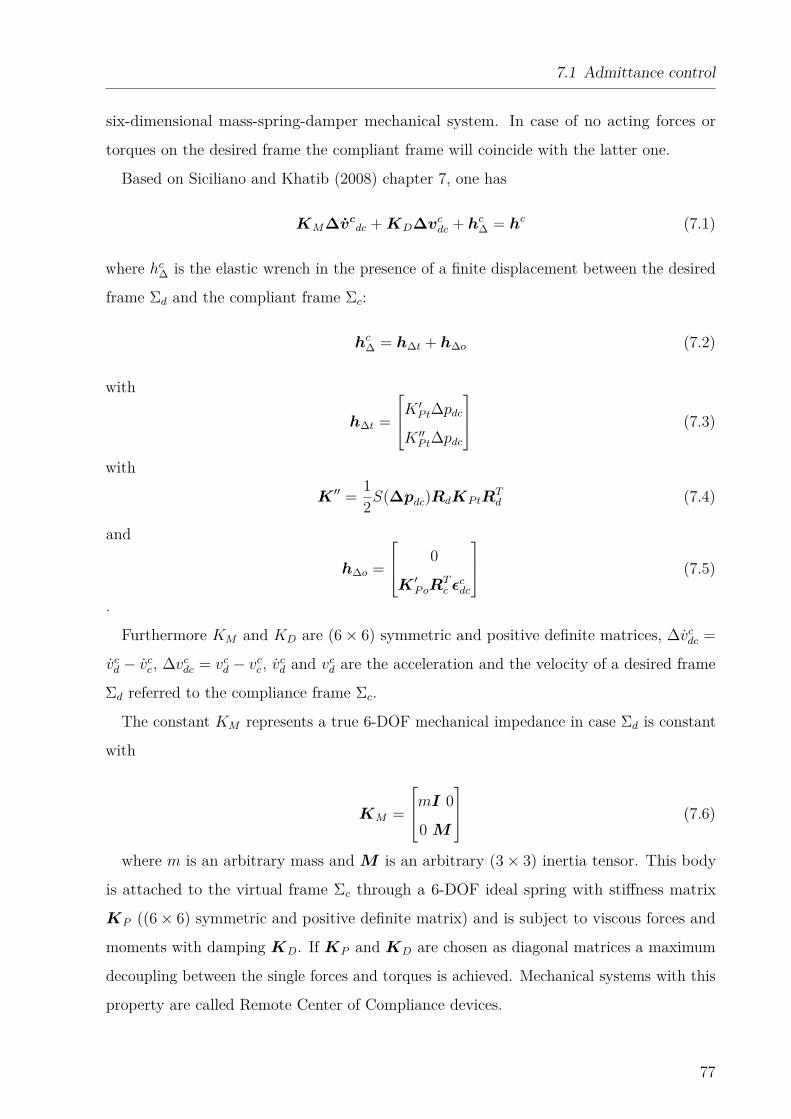
7.1 Admittance control
six-dimensional mass-spring-damper mechanical system. In case of no acting forces or
torques on the desired frame the compliant frame will coincide with the latter one.
Based on Siciliano and Khatib (2008) chapter 7, one has
KM∆vcdc +KD∆vcdc + hc∆ = hc (7.1)
where hc∆ is the elastic wrench in the presence of a finite displacement between the desired
frame Σd and the compliant frame Σc:
hc∆ = h∆t + h∆o (7.2)
with
h∆t =
K ′Pt∆pdcK ′′Pt∆pdc
(7.3)
with
K ′′ = 12S(∆pdc)RdKPtR
Td (7.4)
and
h∆o =
0
K ′PoRTc ε
cdc
(7.5)
.
Furthermore KM and KD are (6× 6) symmetric and positive definite matrices, ∆vcdc =
vcd − vcc, ∆vcdc = vcd − vcc, vcd and vcd are the acceleration and the velocity of a desired frame
Σd referred to the compliance frame Σc.
The constant KM represents a true 6-DOF mechanical impedance in case Σd is constant
with
KM =
mI 0
0 M
(7.6)
where m is an arbitrary mass and M is an arbitrary (3× 3) inertia tensor. This body
is attached to the virtual frame Σc through a 6-DOF ideal spring with stiffness matrix
KP ((6× 6) symmetric and positive definite matrix) and is subject to viscous forces and
moments with damping KD. If KP and KD are chosen as diagonal matrices a maximum
decoupling between the single forces and torques is achieved. Mechanical systems with this
property are called Remote Center of Compliance devices.
77
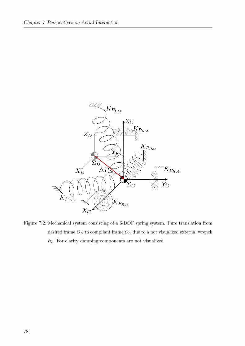
Chapter 7 Perspectives on Aerial Interaction
Figure 7.2: Mechanical system consisting of a 6-DOF spring system. Pure translation from
desired frame OD to compliant frame OC due to a not visualized external wrench
he. For clarity damping components are not visualized
78
7.2 Force Observer
The arbitrary selection of m and M allows a redesign of the dynamical behavior of the
holocopter. The actual mass and inertia are transparent to the interaction task. WithKD =
diag{KDp, KDp, KDp, KDr, KDr, KDr}, KD = diag{KP p, KP p, KP p, KP r, KP r, KP r} and
KM = diag{m,m,m,M1,M2,M3} equation (7.1) results in
mpcx (t)
mpcy (t)
mpcz (t)
M1ocx (t)
M2ocy (t)
M3ocz (t)
=
mpdx (t) +KDp (pdx (t)− pcx (t)) +KP (pdx (t)− pcx (t))− Fx
mpdy (t) +KDp (pdy (t)− pcy (t)) +KP (pdy (t)− pcy (t))− Fy
mpdz (t) +KDp (pdz (t)− pcz (t)) +KP (pdz (t)− pcz (t))− Fz
M1odx (t) +KDr (odx (t)− ocx (t))− τx
M2ody (t) +KDr (ody (t)− ocy (t))− τy
M3odz (t) +KDr (odz (t)− ocz (t))− τz
(7.7)
From (7.7) the decoupling between the single forces and torques becomes clear.
7.2 Force Observer
For closing the control loop knowledge of the reaction force and torques (wrench hc) is
needed. This can be achieved by an onboard force torque sensor inside the end-effector.
However this solution has several drawbacks (Iida and Ohnishi (2003), Katsura et al. (2003)),
amongst others:
• High additional payload for sensor, digital measuring and evaluation system and
mechanics
• Sensor noise: especially a problem on UAVs due to vibrations of the propellers
• Narrow bandwidth: due to vibrations the sensor signals have to be filtered by a low
pass
A possibility to circumvent these problems is the use of a force observer. In a similar
manner the state of a quadrotor is estimated in Benallegue et al. (2006) for the attitude
control and in Jeong et al. (2012) for estimating external disturbances such as wind gusts.
The complete admittance control scheme including an observer is presented in figure 7.3.
79
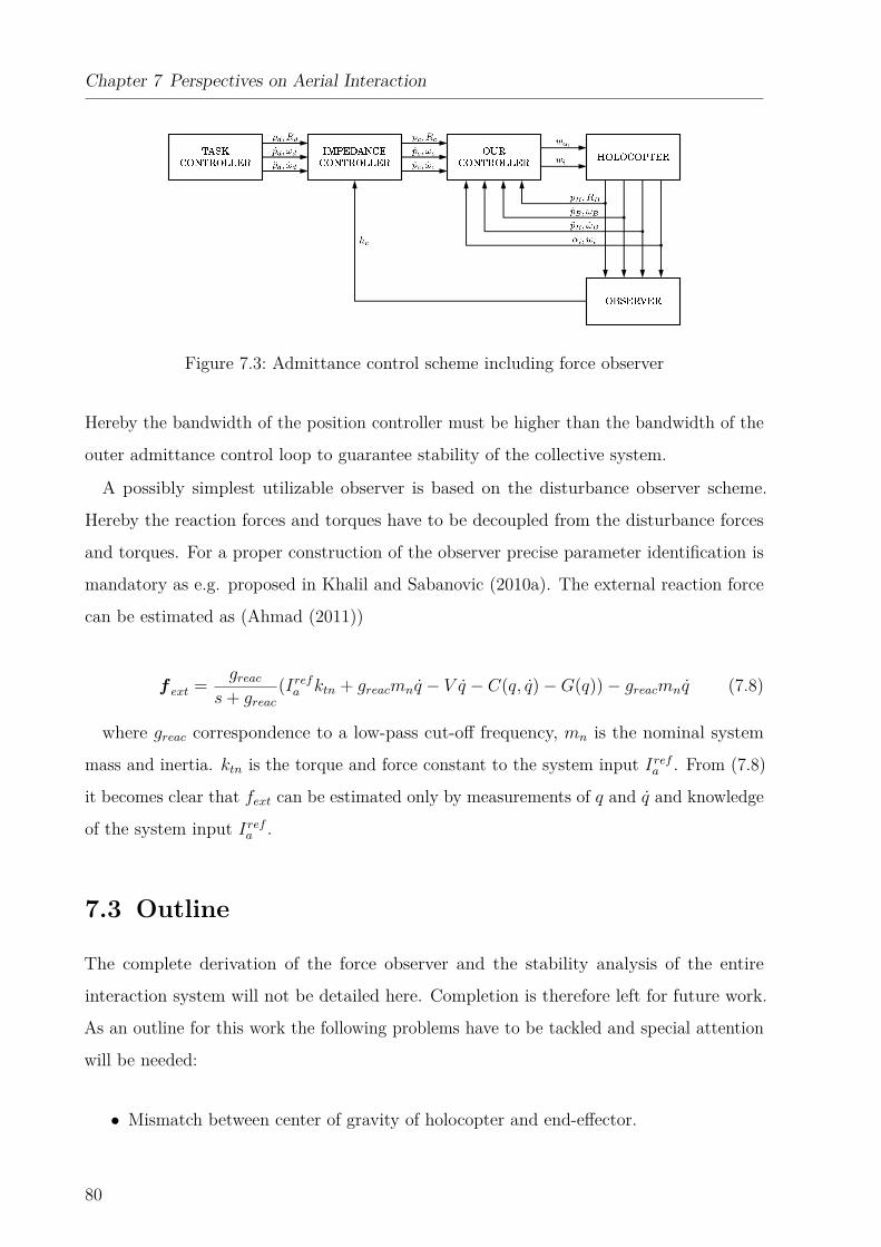
Chapter 7 Perspectives on Aerial Interaction
Figure 7.3: Admittance control scheme including force observer
Hereby the bandwidth of the position controller must be higher than the bandwidth of the
outer admittance control loop to guarantee stability of the collective system.
A possibly simplest utilizable observer is based on the disturbance observer scheme.
Hereby the reaction forces and torques have to be decoupled from the disturbance forces
and torques. For a proper construction of the observer precise parameter identification is
mandatory as e.g. proposed in Khalil and Sabanovic (2010a). The external reaction force
can be estimated as (Ahmad (2011))
f ext = greacs+ greac
(Irefa ktn + greacmnq − V q − C(q, q)−G(q))− greacmnq (7.8)
where greac correspondence to a low-pass cut-off frequency, mn is the nominal system
mass and inertia. ktn is the torque and force constant to the system input Irefa . From (7.8)
it becomes clear that fext can be estimated only by measurements of q and q and knowledge
of the system input Irefa .
7.3 Outline
The complete derivation of the force observer and the stability analysis of the entire
interaction system will not be detailed here. Completion is therefore left for future work.
As an outline for this work the following problems have to be tackled and special attention
will be needed:
• Mismatch between center of gravity of holocopter and end-effector.
80
7.3 Outline
• The bandwidth of the outer loop admittance controller has to be lower than the
bandwidth of the position controller. Additionally the measurements of force observer
are low pass filtered to find a good balance between response and noise attenuation.
These might lead to a low reaction time of the force observer.
• The measurements of q and q together with the parameter identification might not be
accurate to utilize the introduced observer. In this case either an observer without any
sensor information could be used (see Khalil and Sabanovic (2010b)) or a parameter
non-sensitive observer scheme would be required (e.g. sliding mode observer).
81

Chapter 8
Conclusions
In this Ph.D. thesis a novel overactuated quadrotor UAV - the ‘holocopter’ - has been
presented. Exploiting these additional 4 control inputs which yield overactuation, the
holocopter can achieve full controllability over its 6-dof body pose in space. Hereby the
holocopter overcomes the usual limitations of most other UAVs including quadrotors and
helicopters where for any desired trajectory the attitude (roll and pitch) of the UAV is
coupled with its desired position. In the presented concept the ‘holocopter’ 4 additional
degrees of freedom are implemented by individual control of the tilting angles of its four
propellers (vertically fixed for standard quadrotors). This new set of 4 + 4 available control
inputs guarantees as proven in this thesis full controllability over the 6-dimensional pose of
the holocopter main body in space.
In a detailed modeling section the holocopter equations of motion have been derived and
the influence of aerodynamic effects under the desired flight regime has been investigated.
Based on these results a control scheme was developed and adjusted so as to cope with the
practical shortcomings of the first prototype.
A broad variety of ideal and realistic simulations have been conducted, discussed and
reported to assess the effectiveness of the control strategy, to optimize the tuning process
of the various gains and to identify deficits of the first prototype. Satisfactory flight
performances could be presented in a broad variety of real experiments where complex
maneuvers could be presented - impossible for standard quadrotor UAVs.
Additionally the second prototype, a completely revised system has been presented, that
is currently under final software development (see figure 8.1). The new prototype aims
83
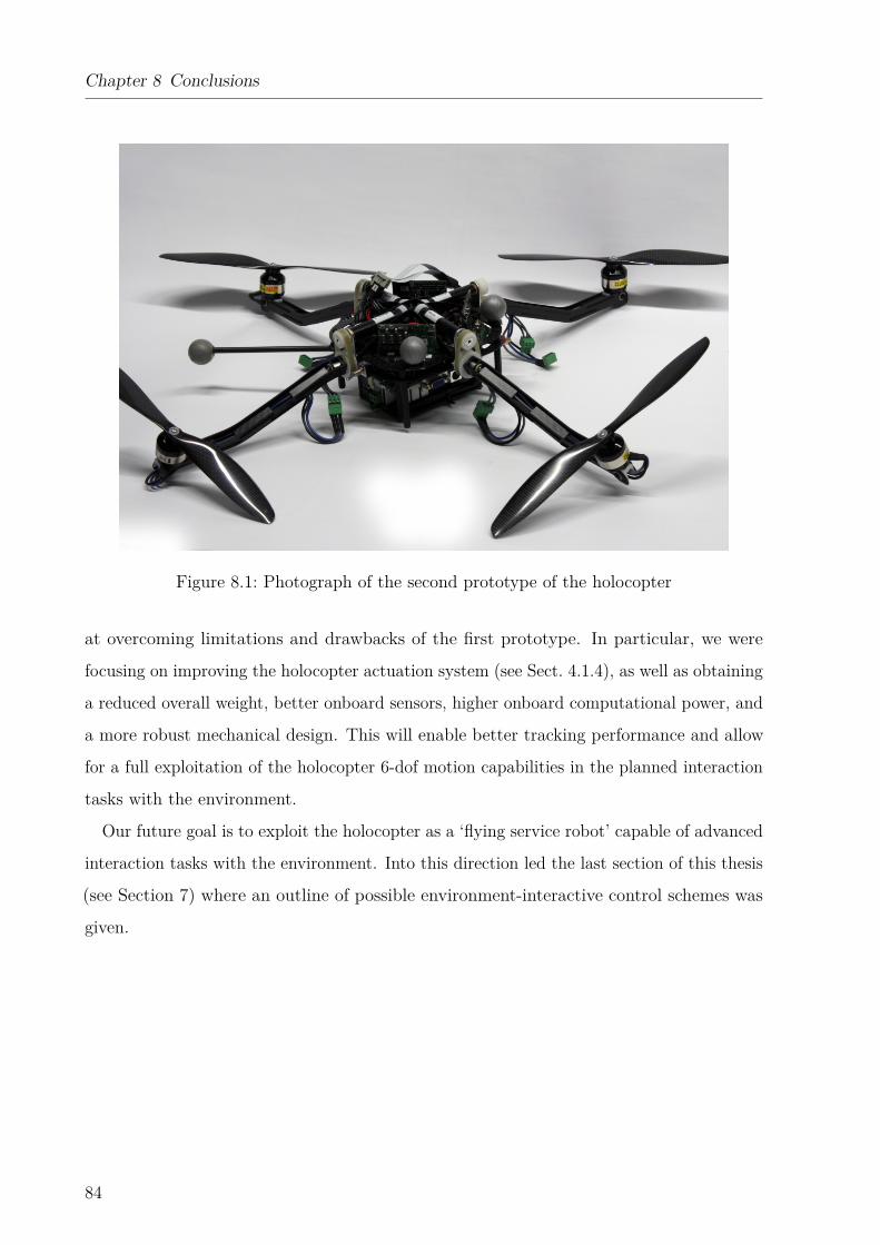
Chapter 8 Conclusions
Figure 8.1: Photograph of the second prototype of the holocopter
at overcoming limitations and drawbacks of the first prototype. In particular, we were
focusing on improving the holocopter actuation system (see Sect. 4.1.4), as well as obtaining
a reduced overall weight, better onboard sensors, higher onboard computational power, and
a more robust mechanical design. This will enable better tracking performance and allow
for a full exploitation of the holocopter 6-dof motion capabilities in the planned interaction
tasks with the environment.
Our future goal is to exploit the holocopter as a ‘flying service robot’ capable of advanced
interaction tasks with the environment. Into this direction led the last section of this thesis
(see Section 7) where an outline of possible environment-interactive control schemes was
given.
84

Appendix
85

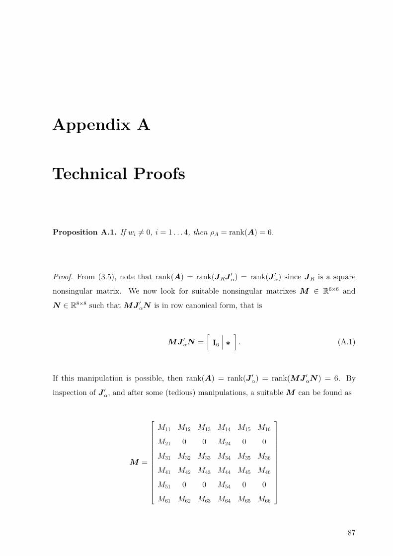
Appendix A
Technical Proofs
Proposition A.1. If wi 6= 0, i = 1 . . . 4, then ρA = rank(A) = 6.
Proof. From (3.5), note that rank(A) = rank(JRJ ′α) = rank(J ′α) since JR is a square
nonsingular matrix. We now look for suitable nonsingular matrixes M ∈ R6×6 and
N ∈ R8×8 such that MJ ′αN is in row canonical form, that is
MJ ′αN =[
I6 ∗]. (A.1)
If this manipulation is possible, then rank(A) = rank(J ′α) = rank(MJ ′αN) = 6. By
inspection of J ′α, and after some (tedious) manipulations, a suitable M can be found as
M =
M11 M12 M13 M14 M15 M16
M21 0 0 M24 0 0
M31 M32 M33 M34 M35 M36
M41 M42 M43 M44 M45 M46
M51 0 0 M54 0 0
M61 M62 M63 M64 M65 M66
87
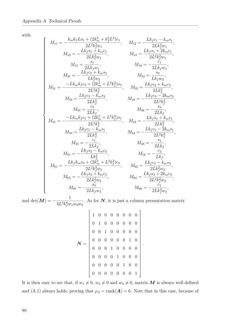
Appendix A Technical Proofs
with
M11 = −kmkfLs1 + (2k2
m + k2fL
2)c1
2L2k3fw1
, M12 = −Lkfc1 − kms1
2Lk2fw1
,
M13 = −Lkfs1 + kmc1
2Lk2fw1
, M14 = Lkfs1 + 2kmc1
2L2k2fw1
,
M15 = s1
2Lkfw1, M16 = − c1
2Lkfw1,
M21 = −Lkfc2 + kms2
Lk2fw2
, M24 = s2
Lkfw2,
M31 = −−Lkmkfc3 + (2k2
m + L2k2f )s3
2L2k3f
, M32 = Lkfs3 + kmc3
2Lk2f
,
M33 = Lkfc3 − kms3
2Lk2f
, M34 = −Lkfc3 − 2kms3
2L2k2f
,
M35 = c3
2Lkf, M36 = − s3
2Lkf,
M41 = −−Lkmkfc1 + (2k2
m + L2k2f )s1
2L2k3f
, M42 = −Lkfs1 + kmc1
2Lk2f
,
M43 = Lkfc1 − kms1
2Lk2f
, M44 = −Lkfc1 − 2kms1
2L2k2f
,
M45 = − c1
2Lkf, M46 = − s1
2Lkf,
M51 = −Lkfs2 − kmc2
Lk2f
, M54 = − c2
Lkf,
M61 = −Lkfkms3 + (2k2
m + L2k2f )c3
2L2k3fw3
, M62 = Lkfc3 − kms3
2Lk2fw3
,
M63 = −Lkfs3 + kmc3
2Lk2fw3
, M64 = Lkfs3 + 2kmc3
2L2k2fw3
,
M65 = − s3
2Lkfw3, M66 = − c1
2Lk2fw3
,
and det(M) = − 14L3k6
fw1w2w3. As for N , it is just a column permutation matrix
N =
1 0 0 0 0 0 0 0
0 1 0 0 0 0 0 0
0 0 1 0 0 0 0 0
0 0 0 0 0 0 1 0
0 0 0 1 0 0 0 0
0 0 0 0 1 0 0 0
0 0 0 0 0 1 0 0
0 0 0 0 0 0 0 1
.
It is then easy to see that, if w1 6= 0, w2 6= 0 and w3 6= 0, matrix M is always well-defined
and (A.1) always holds, proving that ρA = rank(A) = 6. Note that in this case, because of
88
the particular choice made for M , no condition is present on w4 (w4 could vanish). This is
coherent with the intuition that three actuated propellers can be sufficient to provide full
mobility to the quadrotor body (6 inputs for 6 rigid body dofs). However, presence of a
fourth active propeller (w4 6= 0 in this case) guarantees the needed actuation redundancy
exploited in Sect. 3.
89

Appendix B
Schematics
B.1 Mechanical schematics
91
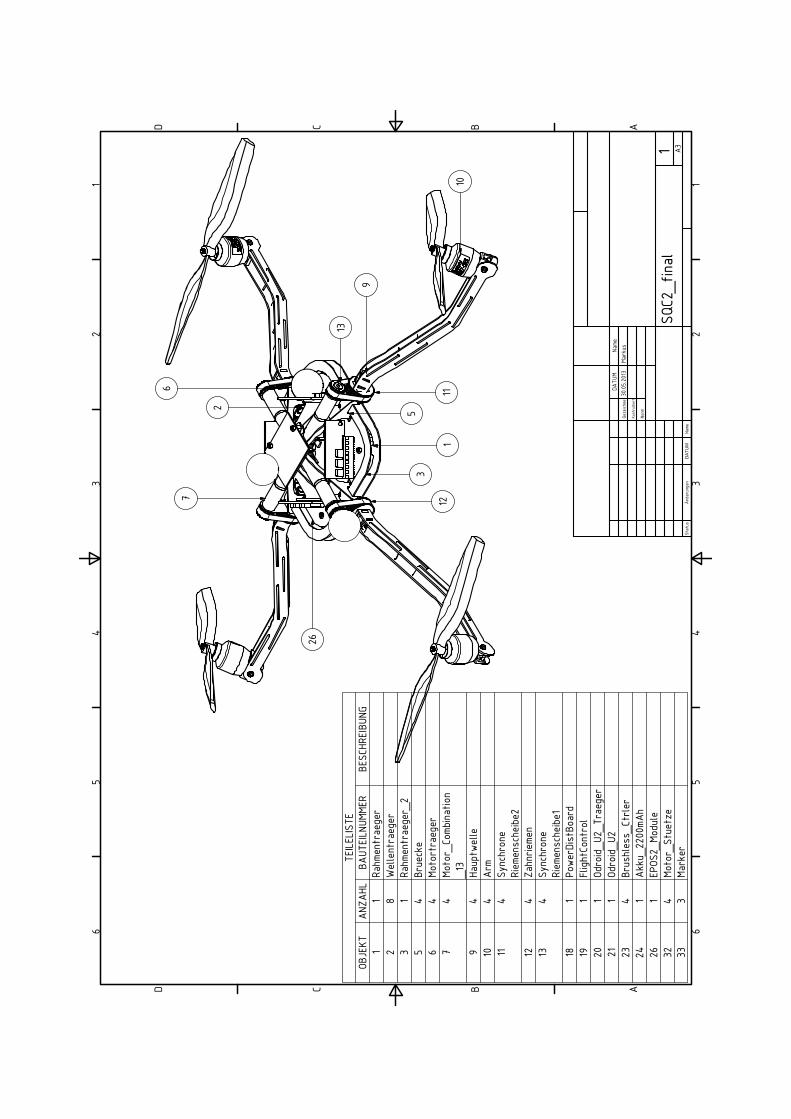
TEILEL
ISTE
BESC
HREIBU
NGBA
UTEILN
UMME
RAN
ZAHL
OBJE
KT
Rahm
entrae
ger
11
Wellent
raeg
er8
2
Rahm
entrae
ger_
21
3
Brue
cke
45
Mo
tortra
eger
46
Mo
tor_
Comb
inat
ion
_13
47
Ha
uptw
elle
49
Ar
m4
10
Sync
hron
e Riem
ensc
heibe2
411
Za
hnrie
men
412
Sy
nchr
one
Riem
ensc
heibe1
413
Po
werD
istB
oard
118
Flight
Cont
rol
119
Od
roid_U
2_Tr
aege
r1
20
Odro
id_U
21
21
Brus
hles
s_Ct
rler
423
Ak
ku_2
200m
Ah1
24
EPOS
2_Mo
dule
126
Mo
tor_
Stue
tze
432
Ma
rker
333
1 1
2 2
3 3
4 4
5 5
6 6
AA
BB
CC
DD
1 A3
SQC2
_final
Stat
usÄn
deru
ngen
DA
TU
MNa
me
Geze
ichne
t
Kont
rollier
t
Norm
DATU
MNa
me30
.05.20
13Ma
rkus
6
9
2
1
3
11
7
10
26
5
13
12
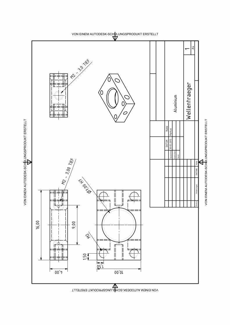
VO
N E
IN
EM
A
UT
OD
ES
K-S
CH
UL
UN
GS
PR
OD
UK
T E
RS
TE
LLT
VO
N E
IN
EM
A
UT
OD
ES
K-S
CH
UL
UN
GS
PR
OD
UK
T E
RS
TE
LLT
VON EINEM AUTODESK-SCHULUNGSPRODUKT ERSTELLTVON EINEM AUTODESK-SCHULUNGSPRODUKT ERSTELLT
1 A4
Wellent
raeg
erSt
atus
Ände
rung
enD
AT
UM
Name
Geze
ichne
t
Kont
rollier
t
Norm
DATU
MNa
me30
.05.20
13Ma
rkus
16,00
4,00 10,00
7,00
H7
1,50
1,50
M2
Alum
inium
M2 -
3,00 TIEF
M2 -
3,0 TIEF
9,00
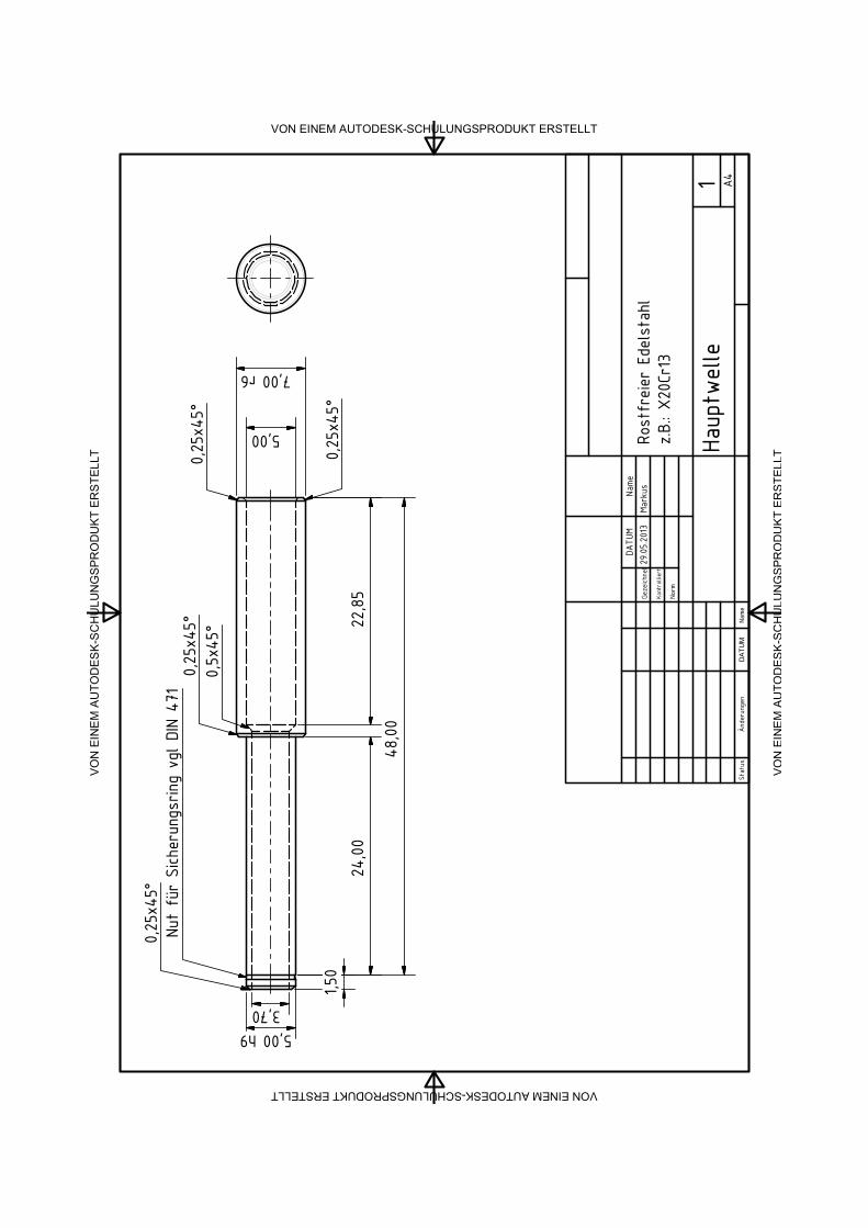
VO
N E
IN
EM
A
UT
OD
ES
K-S
CH
UL
UN
GS
PR
OD
UK
T E
RS
TE
LLT
VO
N E
IN
EM
A
UT
OD
ES
K-S
CH
UL
UN
GS
PR
OD
UK
T E
RS
TE
LLT
VON EINEM AUTODESK-SCHULUNGSPRODUKT ERSTELLTVON EINEM AUTODESK-SCHULUNGSPRODUKT ERSTELLT
1 A4
Haup
twelle
Stat
usÄn
deru
ngen
DA
TU
MNa
me
Geze
ichne
t
Kont
rollier
t
Norm
DATU
MNa
me29
.05.20
13Ma
rkus
7,00 r6
5,00 h9
0,25
x45°
1,50
24,00
48,00
5,00
3,70
22,85
Nut fü
r Sich
erun
gsrin
g vg
l DIN
471
0,5x
45°
0,25
x45°
0,25
x45°
0,25
x45°
Rost
freier
Ede
lsta
hlz.B.: X
20Cr
13
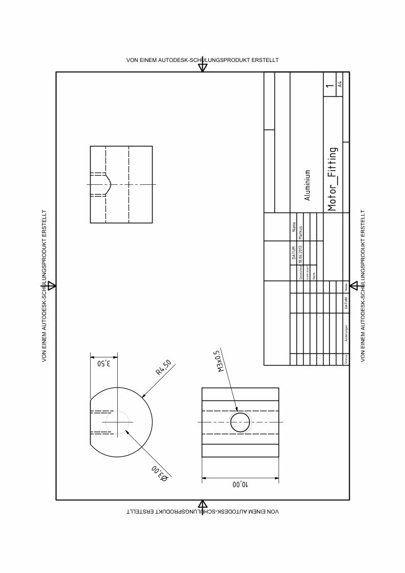
VO
N E
IN
EM
A
UT
OD
ES
K-S
CH
UL
UN
GS
PR
OD
UK
T E
RS
TE
LLT
VO
N E
IN
EM
A
UT
OD
ES
K-S
CH
UL
UN
GS
PR
OD
UK
T E
RS
TE
LLT
VON EINEM AUTODESK-SCHULUNGSPRODUKT ERSTELLTVON EINEM AUTODESK-SCHULUNGSPRODUKT ERSTELLT
1 A4
Moto
r_Fitting
Stat
usÄn
deru
ngen
DA
TU
MNa
me
Geze
ichne
t
Kont
rollier
t
Norm
DATU
MNa
me18
.06.20
13Ma
rkus
10,00
R4,50
3,00
3,50M3
x0.5
Alum
inium
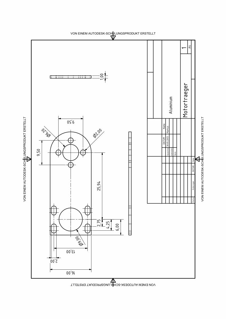
VO
N E
IN
EM
A
UT
OD
ES
K-S
CH
UL
UN
GS
PR
OD
UK
T E
RS
TE
LLT
VO
N E
IN
EM
A
UT
OD
ES
K-S
CH
UL
UN
GS
PR
OD
UK
T E
RS
TE
LLT
VON EINEM AUTODESK-SCHULUNGSPRODUKT ERSTELLTVON EINEM AUTODESK-SCHULUNGSPRODUKT ERSTELLT
1 A4
Moto
rtra
eger
Stat
usÄn
deru
ngen
DA
TU
MNa
me
Geze
ichne
t
Kont
rollier
t
Norm
DATU
MNa
me30
.05.20
13Ma
rkus
16,00
25,94
1,00
2,00
13,00
9,00
2,75
4,25
6,00
2,006,20
Alum
inium
9,50
9,50
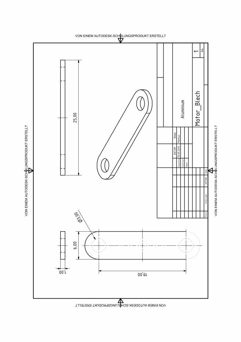
VO
N E
IN
EM
A
UT
OD
ES
K-S
CH
UL
UN
GS
PR
OD
UK
T E
RS
TE
LLT
VO
N E
IN
EM
A
UT
OD
ES
K-S
CH
UL
UN
GS
PR
OD
UK
T E
RS
TE
LLT
VON EINEM AUTODESK-SCHULUNGSPRODUKT ERSTELLTVON EINEM AUTODESK-SCHULUNGSPRODUKT ERSTELLT
1 A4
Moto
r_Blec
hSt
atus
Ände
rung
enD
AT
UM
Name
Geze
ichne
t
Kont
rollier
t
Norm
DATU
MNa
me30
.05.20
13Ma
rkus
3,00
6,00
19,00
25,00
1,00
Alum
inium
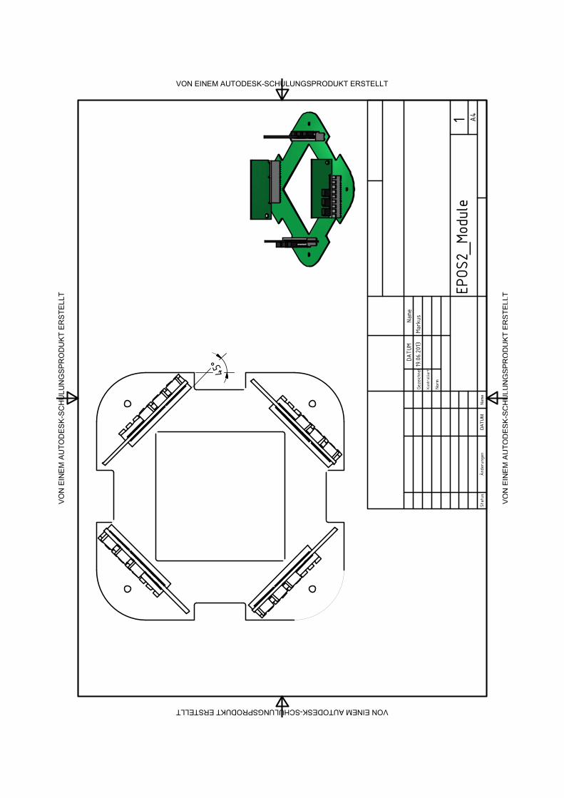
VO
N E
IN
EM
A
UT
OD
ES
K-S
CH
UL
UN
GS
PR
OD
UK
T E
RS
TE
LLT
VO
N E
IN
EM
A
UT
OD
ES
K-S
CH
UL
UN
GS
PR
OD
UK
T E
RS
TE
LLT
VON EINEM AUTODESK-SCHULUNGSPRODUKT ERSTELLTVON EINEM AUTODESK-SCHULUNGSPRODUKT ERSTELLT
1 A4
EPOS
2_Mo
dule
Stat
usÄn
deru
ngen
DA
TU
MNa
me
Geze
ichne
t
Kont
rollier
t
Norm
DATU
MNa
me19
.06.20
13Ma
rkus
45°
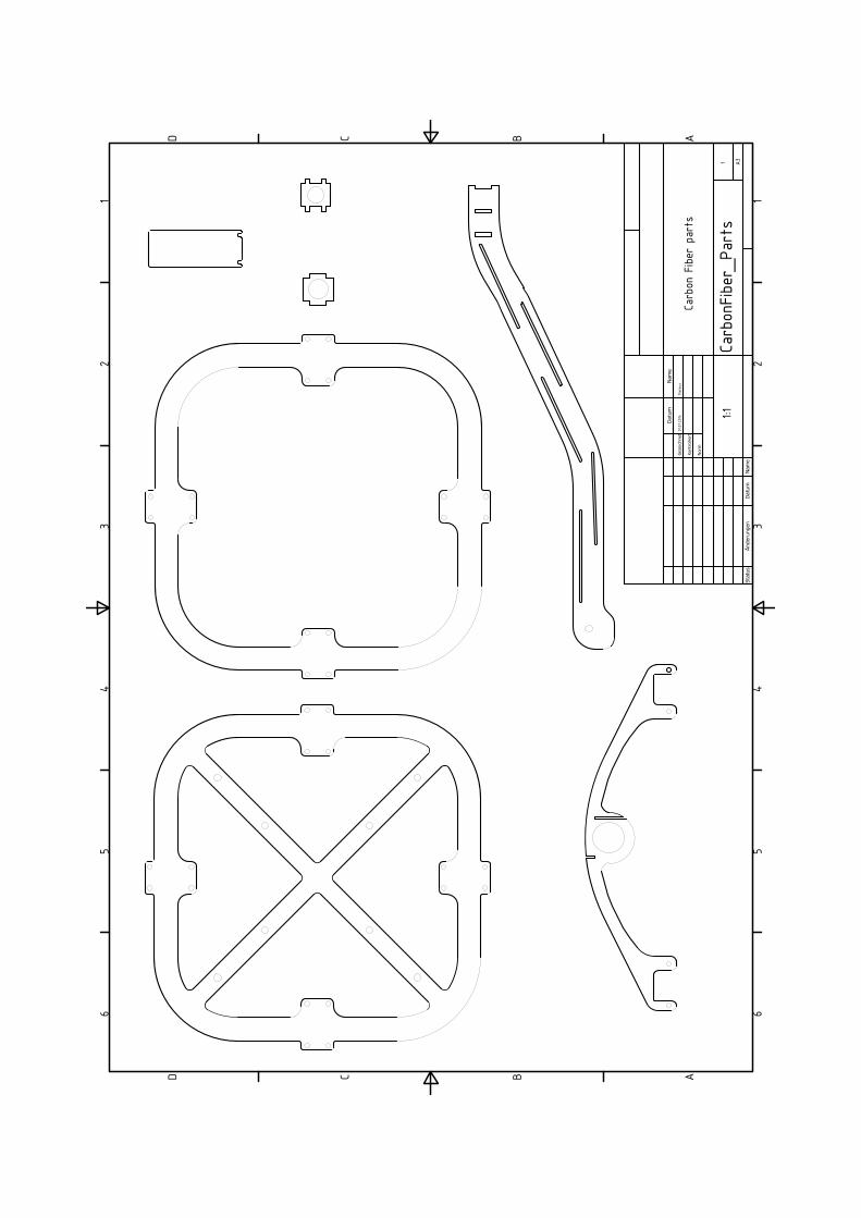
1 1
2 2
3 3
4 4
5 5
6 6
AA
BB
CC
DD
1 A3Ca
rbon
Fibe
r_Pa
rts
Status
Änderungen
Datum
Nam
e
Gezeichnet
Kontrolliert
Norm
Datum
Nam
e
01.07.20
14Ma
rkus
Carb
on F
iber
par
ts
1:1
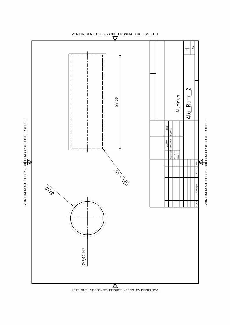
VO
N E
IN
EM
A
UT
OD
ES
K-S
CH
UL
UN
GS
PR
OD
UK
T E
RS
TE
LLT
VO
N E
IN
EM
A
UT
OD
ES
K-S
CH
UL
UN
GS
PR
OD
UK
T E
RS
TE
LLT
VON EINEM AUTODESK-SCHULUNGSPRODUKT ERSTELLTVON EINEM AUTODESK-SCHULUNGSPRODUKT ERSTELLT
1 A4
Alu_
Rohr
_2St
atus
Ände
rung
enD
AT
UM
Name
Geze
ichne
t
Kont
rollier
t
Norm
DATU
MNa
me19
.06.20
13Ma
rkus
Alum
inium
8,50
7,00
H7
22,00
0,30 X 45°
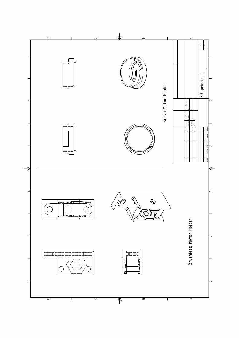
1 1
2 2
3 3
4 4
5 5
6 6
AA
BB
CC
DD
1 A33D
_prin
ter_
IStatus
Änderungen
Datum
Nam
e
Gezeichnet
Kontrolliert
Norm
Datum
Nam
e
01.07.20
14Ma
rkus
Brus
hles
s Mo
tor Ho
lder
Serv
o Mo
tor Ho
lder
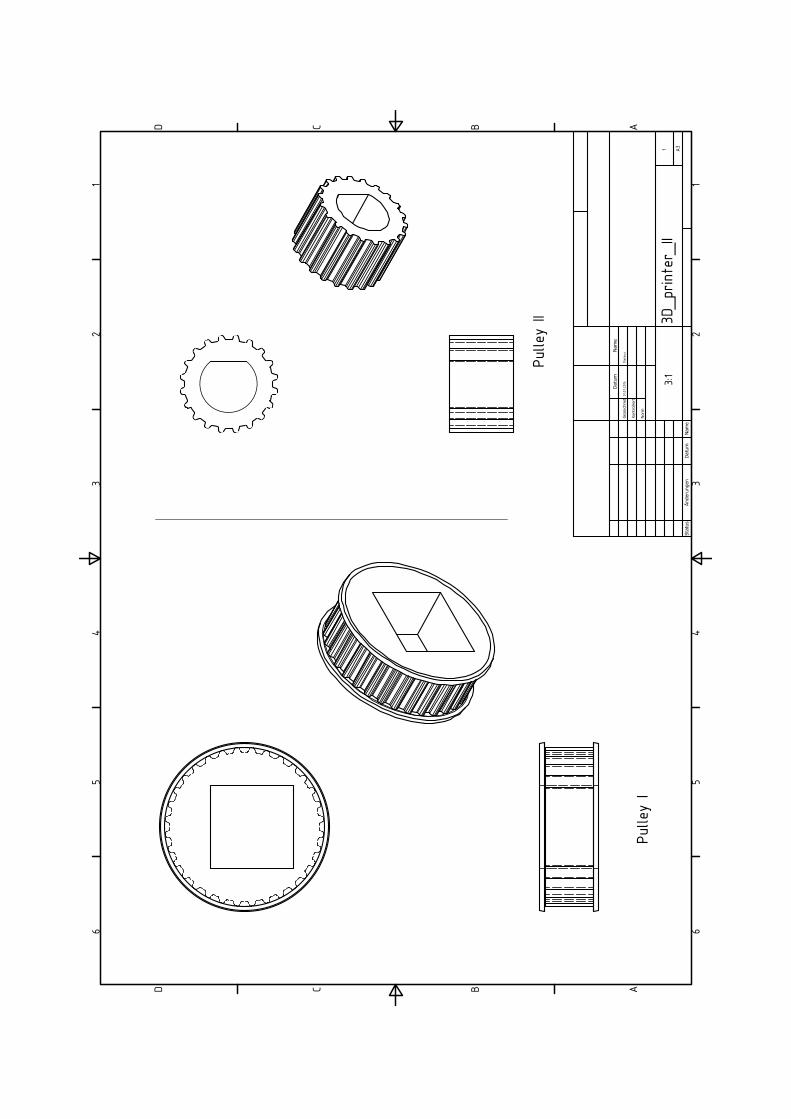
1 1
2 2
3 3
4 4
5 5
6 6
AA
BB
CC
DD
1 A33D
_prin
ter_
IIStatus
Änderungen
Datum
Nam
e
Gezeichnet
Kontrolliert
Norm
Datum
Nam
e
01.07.20
14Ma
rkus
Pulle
y I
Pulle
y II
3:1

B.2 Electrical schematics
B.2 Electrical schematics
103
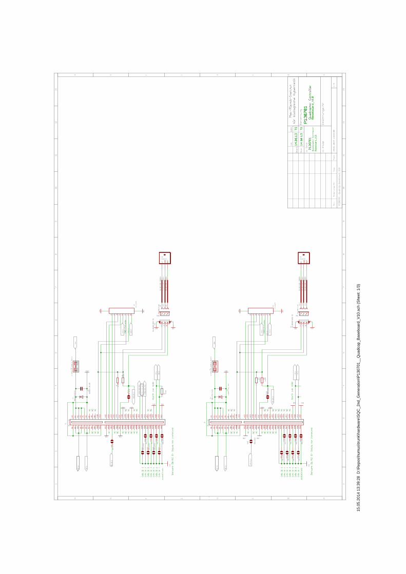
15.0
5.20
14 1
3:39
:28
D:\R
epos
\hum
us\tr
unk\
hard
war
e\S
QC
_2nd
_Gen
erat
ion\
P13
0701
__Q
uadc
op_B
aseb
oard
_V10
.sch
(She
et: 1
/3)
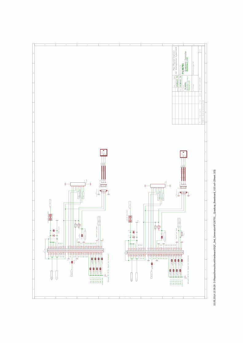
15.0
5.20
14 1
3:39
:29
D:\R
epos
\hum
us\tr
unk\
hard
war
e\S
QC
_2nd
_Gen
erat
ion\
P13
0701
__Q
uadc
op_B
aseb
oard
_V10
.sch
(She
et: 2
/3)
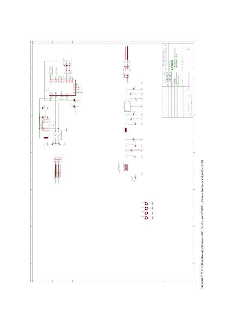
15.0
5.20
14 1
3:39
:29
D:\R
epos
\hum
us\tr
unk\
hard
war
e\S
QC
_2nd
_Gen
erat
ion\
P13
0701
__Q
uadc
op_B
aseb
oard
_V10
.sch
(She
et: 3
/3)
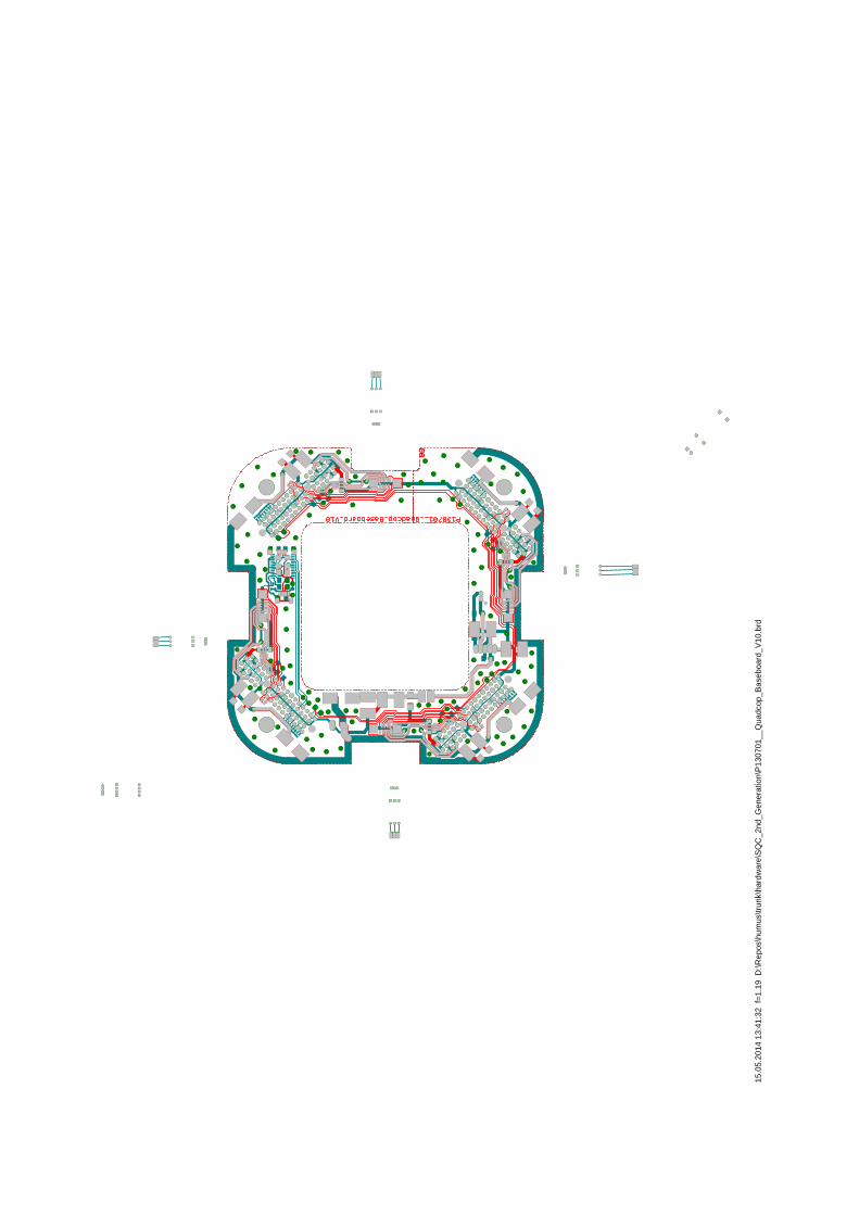
15.0
5.20
14 1
3:41
:32
f=1.
19 D
:\Rep
os\h
umus
\trun
k\ha
rdw
are\
SQ
C_2
nd_G
ener
atio
n\P
1307
01__
Qua
dcop
_Bas
eboa
rd_V
10.b
rd

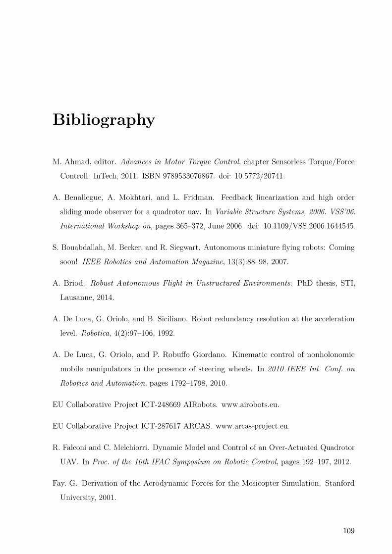
Bibliography
M. Ahmad, editor. Advances in Motor Torque Control, chapter Sensorless Torque/Force
Controll. InTech, 2011. ISBN 9789533076867. doi: 10.5772/20741.
A. Benallegue, A. Mokhtari, and L. Fridman. Feedback linearization and high order
sliding mode observer for a quadrotor uav. In Variable Structure Systems, 2006. VSS’06.
International Workshop on, pages 365–372, June 2006. doi: 10.1109/VSS.2006.1644545.
S. Bouabdallah, M. Becker, and R. Siegwart. Autonomous miniature flying robots: Coming
soon! IEEE Robotics and Automation Magazine, 13(3):88–98, 2007.
A. Briod. Robust Autonomous Flight in Unstructured Environments. PhD thesis, STI,
Lausanne, 2014.
A. De Luca, G. Oriolo, and B. Siciliano. Robot redundancy resolution at the acceleration
level. Robotica, 4(2):97–106, 1992.
A. De Luca, G. Oriolo, and P. Robuffo Giordano. Kinematic control of nonholonomic
mobile manipulators in the presence of steering wheels. In 2010 IEEE Int. Conf. on
Robotics and Automation, pages 1792–1798, 2010.
EU Collaborative Project ICT-248669 AIRobots. www.airobots.eu.
EU Collaborative Project ICT-287617 ARCAS. www.arcas-project.eu.
R. Falconi and C. Melchiorri. Dynamic Model and Control of an Over-Actuated Quadrotor
UAV. In Proc. of the 10th IFAC Symposium on Robotic Control, pages 192–197, 2012.
Fay. G. Derivation of the Aerodynamic Forces for the Mesicopter Simulation. Stanford
University, 2001.
109
Bibliography
J. Fink, N. Michael, S. Kim, and V. Kumar. Planning and control for cooperative
manipulation and transportation with aerial robots. Intern. Journal of Robotics Research,
30(3), 2010.
F. Forte, R. Naldi, A. Macchelli, and L. Marconi. Impedance control of an aerial manipulator.
In American Control Conference (ACC), 2012, pages 3839–3844, June 2012a.
F. Forte, R. Naldi, A. Serrani, and L. Marconi. Control of Modular Aerial Robots:
Combining Under- and Fully-Actuated Behaviors. In 2012 IEEE Conf. on Decision and
Control, pages 1160–1165, 2012b.
A. Franchi, C. Secchi, M. Ryll, H. H. Bülthoff, and P. Robuffo Giordano. Shared control:
Balancing autonomy and human assistance with a group of quadrotor uavs. IEEE
Robotics and Automation Magazine, 19(3):57–68, 2012.
L. Gentili, R. Naldi, and L. Marconi. Modelling and control of VTOL UAVs interacting
with the environment. In 2008 IEEE Conf. on Decision and Control, pages 1231–1236,
2008.
G. Gioioso, M. Ryll, D. Prattichizzo, H. Bülthoff, and A. Franchi. Turning a near-hovering
controlled quadrotor into a 3d force effector. ICRA 2013, 2013.
G. Gioioso, M. Ryll, D. Prattichizzo, H. H. Bülthoff, and A. Franchi. Turning a near-
hovering controlled quadrotor into a 3d force effector. In 2014 IEEE Int. Conf. on
Robotics and Automation, Hong Kong, China, 05/2014 2014.
GmbH HiSystems. Available: http://www.mikrokopter.de. online, 6 2014.
D. Gurdan, J. STumpf, M. Achtelik, K.-M. Dorh, G. Hirzinger, and D. Rus. Energy-efficient
autonomous four-rotor flying robot controlled at 1 kHz. In 2007 IEEE Int. Conf. on
Robotics and Automation, pages 361–366, 2007.
M.-D. Hua, T. Hamel, P. Morin, and C. Samson. A Control Approach for Thrust-Propelled
Underactuated Vehicles and its Application to VTOL Drones. IEEE Trans. on Automatic
Control, 54(8):1837–1853, 2009.
110
Bibliography
M.-D. Hua, T. Hamel, P. Morin, and C. Samson. Introduction to feedback control of
underactuated vtol vehicles: A review of basic control design ideas and principles. IEEE
Control System Magazine, 33(1):61–75, 2013a.
M.-D. Hua, T. Hamel, and C. Samson. Control of VTOL Vehicles with Thrust-direction
Tilting. arXiv:1308.0191, 2013b.
W. Iida and K. Ohnishi. Sensorless force control with force error observer. In Industrial
Technology, 2003 IEEE International Conference on, volume 1, pages 157–162 Vol.1, Dec
2003. doi: 10.1109/ICIT.2003.1290260.
A. Isidori. Nonlinear Control Systems. Springer, 3rd edition, 1995.
S. Jeong, S. Jung, and M. Tomizuka. Attitude control of a quad-rotor system using an
acceleration-based disturbance observer: An empirical approach. In Advanced Intelligent
Mechatronics (AIM), 2012 IEEE/ASME International Conference on, pages 916–921,
July 2012. doi: 10.1109/AIM.2012.6265965.
S. Katsura, Y. Matsumoto, and K. Ohnishi. Modeling of force sensing and validation of
disturbance observer for force control. In Industrial Electronics Society, 2003. IECON
’03. The 29th Annual Conference of the IEEE, volume 1, pages 291–296 vol.1, Nov 2003.
doi: 10.1109/IECON.2003.1279994.
F. Kendoul, I. Fantoni, and R. Lozano. Modeling and control of a small autonomous aircraft
having two tilting rotors. IEEE Trans. on Robotics, 22(6):1297–1302, 2006.
I. Khalil and A. Sabanovic. Action-reaction based parameters identification and states
estimation of flexible systems. In Industrial Electronics (ISIE), 2010 IEEE International
Symposium on, pages 46–51, July 2010a. doi: 10.1109/ISIE.2010.5637217.
I. Khalil and A. Sabanovic. Sensorless action-reaction-based residual vibration suppression
for multi-degree-of-freedom flexible systems. In IECON 2010 - 36th Annual Conference
on IEEE Industrial Electronics Society, pages 1633–1638, Nov 2010b. doi: 10.1109/
IECON.2010.5675440.
A. Kushleyev, D. Mellinger, and V. Kumar. Towards A Swarm of Agile Micro Quadrotors.
In 2012 Robotics: Science and Systems, 2012.
111
Bibliography
T. Lee, M. Leok, and N. H. McClamroch. Geometric tracking control of a quadrotor UAV
on SE(3). In 2010 IEEE Conf. on Decision and Control, pages 5420–5425, 2010.
Q. Lindsey, D. Mellinger, and V. Kumar. Construction of cubic structures with quadrotor
teams. In Robotics: Science and Systems, 2011.
Y. Long and D. J. Cappelleri. Linear Control Design, Allocation, and Implementation for
the Omnicopter MAV. In 2013 IEEE Int. Conf. on Robotics and Automation, pages
289–294, 2013.
R. Mahony, V. Kumar, and P. Corke. Multirotor aerial vehicles: Modeling, estimation, and
control of quadrotor. IEEE Robotics & Automation Magazine, 19(3):20–32, 2012.
M. Manubens, D. Devaurs, L. Ros, and J. Cortés. Motion Planning for 6-D Manipulation
with Aerial Towed-cable Systems. In 2013 Robotics: Science and Systems, Berlin,
Germany, June 2013.
L. Marconi and R. Naldi. Control of aerial robots. hybrid force/position feedback for a
ducted-fan. IEEE Control System Magazine, 32(4):43–65, 2012.
D. Mellinger and V. Kumar. Minimum snap trajectory generation and control for quadrotors.
In 2011 IEEE Int. Conf. on Robotics and Automation, pages 2520–2525, 2011.
D. Mellinger, N. Michael, and V. Kumar. Trajectory generation and control for precise ag-
gressive maneuvers with quadrotors. In Proc. of the 2010 Int. Symposium on Experimental
Robotics, 2010.
N. Michael, J. Fink, and V. Kumar. Cooperative manipulation and transportation with
aerial robots. In Robotics: Science and Systems, Seattle, USA, June 2009.
R. Naldi and L. Marconi. Modeling and control of the interaction between flying robots
and the environment. In Proc. of the 2010 IFAC NOLCOS, 2010.
R. Naldi, L. Gentili, L. Marconi, and A. Sala. Design and experimental validation of a
nonlinear control law for a ducted-fan miniature aerial vehicle. Control Engineering
Practice, 18(7):747–760, 2010.
112
Bibliography
K. T. Oner, E. Cetinsoy, M. Unel, M. F. Aksit, I. Kandemir, and K. Gulez. Dynamic model
and control of a new quadrotor unmanned aerial vehicle with tilt-wing mechanism. In
Proc. of the 2008 World Academy of Science, Engineering and Technology, pages 58–63,
2008.
K. T. Oner, E. Cetinsoy, E. Sirimoglu, C. Hancer, T. Ayken, and M. Unel. LQR and SMC
stabilization of a new unmanned aerial vehicle. In Proc. of the 2009 World Academy of
Science, Engineering and Technology, pages 554–559, 2009.
OpenServo.org. Available: http://openservo.com. online, 6 2014.
P. E. I. Pound, D. R. Bersak, and A. M. Dollar. Grasping from the air: Hovering capture
and load stability. In 2011 IEEE Int. Conf. on Robotics and Automation, pages 2491–2498,
2011.
P. Pounds, R. Mahony, and P. Corke. Modelling and control of a large quadrotor robot.
Control Engineering Practice, 18(7):691–699, 2010.
robbe Modellsport GmbH & Co. KG. Available: http://www.robbe.de/servo-s-3150-
digital.html. online, 6 2014.
M. Ryll, H. H. Bülthoff, and P. Robuffo Giordano. Modeling and Control of a Quadrotor
UAV with Tilting Propellers. In 2012 IEEE Int. Conf. on Robotics and Automation,
pages 4606–4613, 2012.
M. Ryll, H. H. Bülthoff, and P. Robuffo Giordano. First Flight Tests for a Quadrotor UAV
with Tilting Propellers. In 2013 IEEE Int. Conf. on Robotics and Automation, pages
295–302, 2013.
M. Ryll, H. H. Bülthoff, and P. Robuffo Giordano. A novel overactuated quadrotor uav:
Modeling, control and experimental validation. IEEE Transactions on Control Systems
Technology, to be published 2014.
A. Sanchez, J. Escareño, O. Garcia, and R. Lozano. Autonomous hovering of a noncyclic
tiltrotor UAV: Modeling, control and implementation. In Proc. of the 17th IFAC Wold
Congress, pages 803–808, 2008.
113
Bibliography
S. Shen, Y. Mulgaonkar, N. Michael, and V. Kumar. Vision-Based State Estimation and
Trajectory Control Towards High-Speed Flight with a Quadrotor. In 2013 Robotics:
Science and Systems, 2013.
B. Siciliano and O. Khatib, editors. Handbook of Robotics, chapter Force Control. Springer,
2008. ISBN 9783540239574.
R. Spica, A. Franchi, G. Oriolo, H. H. Bülthoff, and P. Robuffo Giordano. Aerial Grasping
of a Moving Target with a Quadrotor UAV. In 2012 IEEE/RSJ Int. Conf. on Intelligent
Robots and Systems, pages 4985–4992, 2012.
K. Sreenath and V. Kumar. Dynamics, Control and Planning for Cooperative Manipulation
of Payloads Suspended by Cables from Multiple Quadrotor Robots. In 2013 Robotics:
Science and Systems, 2013.
W. Stepniewski and C. Keys, editors. Rotary-Wing Aerodynamics. Dover Publications,
1984.
K. P. Valavanis, editor. Advances in Unmanned Aerial Vehicles: State of the Art and the
Road to Autonomy. Springer, 2007.
R. Voyles and G. Jiang. Hexrotor uav platform enabling dextrous interaction with structures
- preliminary work. In Safety, Security, and Rescue Robotics (SSRR), 2012 IEEE
International Symposium on, pages 1–7, 2012.
W. A. Wolovich. Automatic Control Systems. Oxford University Press, 1994.
114