Landmark Feature Signatures for UAV Navigation

Aakash Dawadee, Javaan Chahl, D(Nanda) Nandagopal and Zorica Nedic

Division of IT, Engineering and the Environment

University of South Australia (UniSA)

Mawson Lakes, SA, Australia

Email: {Aakash.Dawadee, Javaan.Chahl, Nanda.Nandagopal, Zorica.Nedic}@unisa.edu.au

Abstract—We present a landmark detection method for vision-

based Unmanned Aerial Vehicle (UAV) navigation. An image is

normalized and a reference point is taken as the intersection of

two major edges on the image. A number of objects are then

extracted and their centroids are computed. Sections of image

covering landmarks are circularly cropped from the normalized

image with their center as centroid of landmarks. For each pixel

on the border of cropped section, a line is drawn from the center.

We represent landmark feature signature as summation of all

pixels along the lines. These feature signatures are unique for

different objects and hence can be used for landmark detection

for navigation of UAVs. Our results show successful detection of

landmarks on simulated images as well as real images. The

results also show that the algorithm is robust against large

variation in illumination, rotation and scale.

Keywords—Unmanned Aerial Vehicle; Landmark; Feature

Signature.

I. INTRODUCTION

The autonomy level of UAVs has been growing dramatically over the past few years due to advances in technologies that underpin autonomous system. Complete and reliable navigation of unmanned systems is achieved with the use of active sensors such as Radio Frequency (RF) and Global Positioning System (GPS) [1]. Despite the success of active methods, there is a growing interest in passive methods such as vision. Recently, passive vision methods have been proposed to assist GPS systems to mitigate GPS outage problems [2], [3]. Over the years, systems have been developed with GPS and vision combined with sensors such as Inertial Measurement Unit (IMU), Pressure Sensor Altimeter (PSA) etc. [4], [5], [6]. These systems rely on active navigation methods and cannot be guaranteed against jamming or spoofing. Hence, a completely passive system would be advantageous if it was feasible. A vision-based system is a strong candidate for building fully passive navigation. In vision-based navigation, it is of critical importance to correctly identify landmarks in the terrain. In this paper, we present a method that could be used for landmark identification for vision-based UAV navigation. A significant amount of research has been carried out over the past few years in the fields of object detection and image matching. In the next section, we present a brief overview of current state of the art of object detection approaches. The proposed feature signature computation algorithm is described in Section III, followed by results in section IV, discussions in section V and conclusion / future work in section VI.

II. LITERATURE REVIEW: OBJECT DETECTION

Online Robot Landmark Processing System (RLPS) was

developed to detect, classify and localize different types of

objects during robot navigation [7]. A single camera model for

extraction and recognition of visual landmarks was described

in [8] where quadrangular landmarks were used for indoor

navigation. Landmarks were extracted during environment

exploration and robot was navigating by searching those

landmarks to localize itself. Madhavan and Durrant-Whyte [9]

described an algorithm for UGV navigation with the aid of

natural landmarks in unstructured environments. This

algorithm used maximum curvature points with laser scan data

as point landmarks. Then, a Curvature Scale Space (CSS)

algorithm was developed and used to locate maximum

curvature points. Eventually, these points are combined in an

Extended Kalman Filter (EKF) to determine location of the

vehicle. Google-earth imagery simulating a camera was used

for the autonomous navigation of UAVs [10]. In this work

authors proposed the landmark recognition algorithm for UAV

navigation with the use of current Geo-systems such as

Google-earth which excludes gathering of complex data from

sensors. Wu and Tsai [11] used Omni-directional vision with

artificial circular landmarks on ceilings to provide location

estimation for an indoor autonomous system. Cesetti et al. [12]

proposed a landmark matching method for vision based

guidance and safe landing of UAVs.

III. ALGORITHM DESCRIPTION: FEATURE SIGNATURE

We propose a novel approach to represent features of a landmark from a grayscale image as a one-dimensional signature vector. An image represented by a two-dimensional function such as I(X,Y) is mapped to a sub-space i(x,y) within the image.

I(X,Y) → i(x,y). (1)

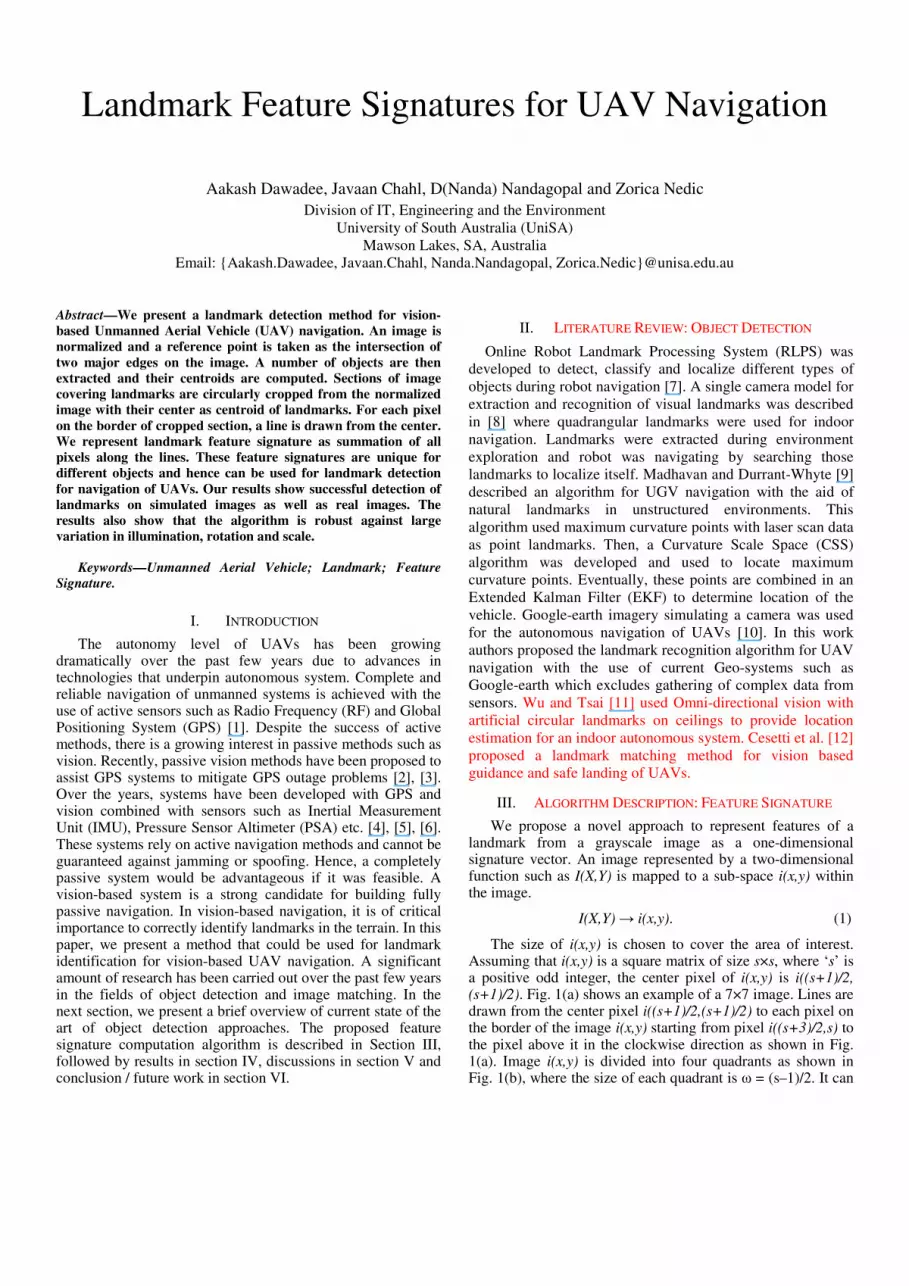
The size of i(x,y) is chosen to cover the area of interest. Assuming that i(x,y) is a square matrix of size s×s, where ‘s’ is a positive odd integer, the center pixel of i(x,y) is i((s+1)/2, (s+1)/2). Fig. 1(a) shows an example of a 7×7 image. Lines are drawn from the center pixel i((s+1)/2,(s+1)/2) to each pixel on the border of the image i(x,y) starting from pixel i((s+3)/2,s) to the pixel above it in the clockwise direction as shown in Fig. 1(a). Image i(x,y) is divided into four quadrants as shown in Fig. 1(b), where the size of each quadrant is ω = (s–1)/2. It can

be observed that there are 2ω lines in each quadrant. For each quadrant, a set of equations is formulated.

Figure 1: (a) An image with 7×7 pixels; (b) Four quadrants of an image.

i. Angles made by ω lines with:

horizontal axis at the center pixel for the first and third quadrants or vertical axis at the center pixel for second and fourth quadrants,

1tan , {1, 2,..., }.i

iiθ ω

ω

− = ∈

(2)

ii. Angles made by remaining ω lines with:

vertical axis at the center pixel for the first and third quadrants or horizontal axis at the center pixel for the second and fourth quadrants,

1tan , {1, 2,..., }.i

ii

ωφ ω

ω

− − = ∈

(3)

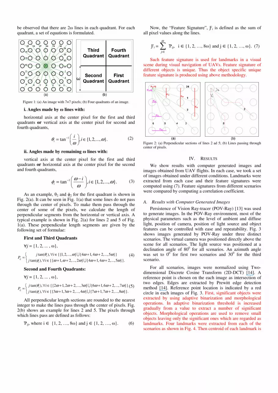
As an example, θ2 and ϕ2 for the first quadrant is shown in Fig. 2(a). It can be seen in Fig. 1(a) that some lines do not pass through the center of pixels. To make them pass through the center of some of the pixels, we calculate the length of perpendicular segments from the horizontal or vertical axis. A typical example is shown in Fig. 2(a) for lines 2 and 5 of Fig. 1(a). These perpendicular length segments are given by the following set of formulae:

First and Third Quadrants

∀j = {1, 2, ... , ω},

tan( ), {{1, 2,..., } {4 1, 4 2,...,5 }}

tan( ), {{ 1, 2,..., 2 } {4 1,4 2,...,5 }}.

i

ij

i

j iP

j i

θ ω ω ω ω

φ ω ω ω ω ω ω

∀ ∈ + +=

∀ ∈ + + + +

∪

∪

(4)

Second and Fourth Quadrants:

∀j = {1, 2, ... , ω},

tan( ), {{2 1, 2 2,...,3 } {6 1,6 2,..., 7 }}

tan( ), {{3 1,3 2,..., 4 } {7 1,7 2,...,8 }}.

i

ij

i

j iP

j i

θ ω ω ω ω ω ω

φ ω ω ω ω ω ω

∀ ∈ + + + +=

∀ ∈ + + + +

∪

∪

(5)

All perpendicular length sections are rounded to the nearest integer to make the lines pass through the center of pixels. Fig. 2(b) shows an example for lines 2 and 5. The pixels through which lines pass are defined as follows:

Ƥij, where i ∈ {1, 2, …, 8ω} and j ∈{1, 2, …, ω}. (6)

Now, the “Feature Signature”, Ƒi is defined as the sum of all pixel values along the lines.

Ƒi =

1j

ω

=

∑ Ƥij, i ∈{1, 2, …, 8ω} and j ∈{1, 2, …, ω}. (7)

Such feature signature is used for landmarks in a visual scene during visual navigation of UAVs. Feature signature of different objects is unique. Thus the object specific unique feature signature is produced using above methodology.

Figure 2: (a) Perpendicular sections of lines 2 ad 5; (b) Lines passing through center of pixels.

IV. RESULTS

We show results with computer generated images and images obtained from UAV flights. In each case, we took a set of images obtained under different conditions. Landmarks were extracted from each case and their feature signatures were computed using (7). Feature signatures from different scenarios were compared by computing a correlation coefficient.

A. Results with Computer Generated Images

Persistence of Vision Ray-tracer (POV-Ray) [13] was used to generate images. In the POV-Ray environment, most of the physical parameters such as the level of ambient and diffuse light, position of camera, position of light source and object features can be controlled with ease and repeatability. Fig. 3 shows images generated by POV-Ray under three distinct scenarios. The virtual camera was positioned directly above the scene for all scenarios. The light source was positioned at a declination angle of 80

0 for all scenarios. An azimuth angle

was set to 00 for first two scenarios and 30

0 for the third

scenario.

For all scenarios, images were normalized using Two-dimensional Discrete Cosine Transform (2D-DCT) [14]. A reference point is chosen on the each image as intersection of two edges. Edges are extracted by Prewitt edge detection method [14]. Reference point location is indicated by a red circle in each images of Fig. 3. First, significant objects were extracted by using adaptive binarization and morphological operations. In adaptive binarization threshold is increased gradually from a value to extract a number of significant objects. Morphological operations are used to remove small objects leaving only the significant ones which are regarded as landmarks. Four landmarks were extracted from each of the scenarios as shown in Fig. 4. Then centroid of each landmark is

computed and image section covering landmarks are circularly cropped from normalized images. These cropped images were scaled by taking a reference to the camera position to make the algorithm scale-invariant. Each of the circularly cropped section are rotated by bicubic interpolation such that line joining the center of the cropped section and the reference

point lay on positive x-axis as shown in Fig. 5. This was done to make the algorithm rotation-invariant. For all of these objects, the one-dimensional feature signatures were computed using (7) which are shown in Fig. 6. Table 1 shows correlation coefficients between landmark feature signatures of scenario-1 against scenario-2 and 3.

Figure 3: POV-Ray Images. (a) Scenario-1: An image with two lines and four objects taken under good lighting conditions; (b) Scenario-2: Image of Fig. 3(a) under

low lighting conditions; (c) Scenario-3: Image of Fig. 3(a) with two extra lines, random clutter and change in scale/ rotation.

Figure 4: POV-Ray: Landmarks obtained after adaptive binarization and morphological operations. (a) Scenario-1; (b) Scenario-2; (c) Scenario-3.

Figure 5: POV-Ray: Circularly cropped objects extracted from normalized images after rotation. (a) Scenario-1; (b) Scenario-2; (c) Scenario-3.

Figure 6: POV-Ray: Feature Signature of objects from three different scenarios. (a) Scenario-1; (b) Scenario-2; (c) Scenario-3.

B. Results with Real World Field Images

In this section, we show results with images taken by a camera in the field under different illumination, scale and rotation. Images taken under three different scenarios are shown in Fig. 7 with reference point location indicated by red circles. As in the case of computer generated images, images of all three scenarios were normalized using 2D-DCT. Images

were scaled by taking a reference to the camera position to make the algorithm scale-invariant. Objects were circularly cropped from normalized images. Cropped sections were rotated with logic explained in the previous section. Fig. 8 shows cropped sections after rotation. Fig. 9 shows the one-dimensional feature signatures of landmarks. Table 2 shows correlation coefficients between landmark feature signatures of scenario-1 against scenario-2 and 3.

Table 1: POV-Ray Images: Correlation coefficients between landmark feature signatures of scenario-1 against scenario-2 and scenario-3

Scenario-2 Features Scenario-3 Features

Scenario-1

Features

(i) (ii) (iii) (iv) (i) (ii) (iii) (iv)

(i) 0.9925 0.3017 –0.1465 0.6804 0.9876 0.2513 –0.1257 0.6200

(ii) 0.2127 0.9831 0.5881 0.5357 0.2243 0.9655 0.6053 0.5583

(iii) –0.1405 0.5578 0.9966 –0.2855 –0.1176 0.5753 0.9906 –0.2677

(iv) 0.6281 0.5700 –0.2654 0.9995 0.6263 0.5350 –0.2429 0.9787

Figure 7: Real-world Field Images. (a) Scenario-1: An image taken in the field under moderate lighting conditions; (b) Scenario-2: An image taken in the field under

low lighting conditions with change in view angle (rotation) and camera position away from scene (scale); (c) Scenario-3: An image taken in the field under high lighting conditions with change in view angle (rotation), camera position further away from the scene (scale) and introduction of random clutter around the

landmarks.

Figure 8: Real-world Field Images: Circularly cropped objects extracted from normalized images after rotation. (a) Scenario-1; (b) Scenario-2; (c) Scenario-3.

Figure 9: Real-world Field Images: Feature Signature of objects from three different scenarios. (a) Scenario-1; (b) Scenario-2; (c) Scenario-3.

Table 2: Real-world Field Images: Correlation coefficients between landmark feature signatures of scenario-1 against scenario-2 and scenario-3.

Scenario-2 Features Scenario-3 Features

Scenario-1

Features

(i) (ii) (iii) (iv) (v) (vi) (vii) (viii)

(i) 0.8171 0.5559 0.3378 0.4425 0.8761 0.5380 0.2060 0.5670

(ii) 0.6819 0.8666 0.6094 0.4970 0.5749 0.8584 0.4606 0.5699

(iv) 0.2713 0.5990 0.8903 –0.1103 0.2148 0.5060 0.8218 –0.0598

(vi) 0.4898 0.5065 0.0003 0.8351 0.4349 0.5928 –0.1079 0.8281

V. DISCUSSION

For computer generated images, we used three different

scenarios varying in illumination, scale and rotation. The

background was consistent in all cases. This enhanced the

normalization process. There were four significant objects

in the image in all cases which were regarded as landmarks.

Landmark feature signatures from scenario-1 were

compared against those of scenario-2 and 3 by computing

correlation coefficients. As shown in Table 1, feature

signatures corresponding to same objects from different

scenarios had very high correlation whereas those

corresponding to different objects had significantly low

correlation. Although images in three different scenarios

were obtained in different illumination, scale, rotation and

noise (i.e. clutter) conditions, we achieved correlation

coefficients higher than 96% in all cases of matching.

The algorithm was then tested on images obtained from

real world field images. As shown in Fig. 6, images chosen

for three different scenarios were different in terms of

illumination, rotation and scale. In spite of such differing

scenarios, we obtained good correlation between landmark

feature signatures of same objects from different scenarios.

As shown in Table 2, feature signatures (i), (ii), (iii) and (iv)

of scenario-1 (Fig. 9(a)) were correctly matched with

corresponding feature signatures of scenario-2 (Fig. 9(b))

with correlation value greater than 81%. Correlation

coefficients between feature signatures corresponding to

different objects from these two scenarios were significantly

low. Also, features (i), (ii), (iii) and (iv) of scenario-1 were

matched with corresponding features of scenario-3 (Fig.

9(c)) with correlation coefficients greater than 82%. Again,

we obtained low correlation values for different objects

from these two scenarios. Slightly lower values of

correlation coefficients for matched landmark feature

signatures as compared to simulated results were due to

various reasons. Firstly as seen in Fig. 8, view angle in

different scenarios altered the appearance of the objects.

Moreover, slight errors were accumulated during rescaling

and rotation of images. We intend to improve on these

causes in our future work. Nevertheless, we have been able

to correctly match landmarks from vastly differing

scenarios. Identified landmarks can be used to localize an

UAV in the space and used for the navigation.

Method demonstrated in [11] is used for only circular

landmarks whereas our method considers variety of

landmark shapes. Popular method of object matching such

as Scale Invariant Feature Transform (SIFT) [15] are proven

computationally expensive [12]. Our method is simple and

computationally inexpensive and has great potential for real

time application of UAVs. Moreover, landmark matching

approach described in [12] considers single landmark

matching scheme which increases a chance of deadlock

when a matching is not obtained. Our method considers

multiple landmarks that ultimately form a waypoint. Hence,

even though some landmarks are occluded, detected

landmarks could be used to form a waypoint for UAV

navigation.

VI. CONCLUSION AND FUTURE WORK

We presented a method for computing unique one-

dimensional feature signature from terrain images for

landmark recognition. The results demonstrate high

correlation coefficients for the same objects captured in

different scenarios under different conditions. However,

different objects from two scenarios had low correlation as

expected. Further work is underway to improve the

algorithm’s performance to achieve even higher levels of

correlation under more challenging conditions.

ACKNOWLEDGMENT

This research was partially supported by Defense Science and Technology Organization (DSTO), Australia. Their support is greatly appreciated.

REFERENCES

[1] G. Loegering and D. Evans, “ The Evolution of the Global Hawk and MALD Avionics Systems,” in Proceedings of 18th Digital Avionics Systems Converence, IEEE, vol. 2, 1999, pp. 6.A.1–1–6.A.1–8.

[2] M. George and S. Sukkarieh, “Camera Aided Inertial Navigation in Poor GPS Environments,” in IEEE Aerospace Conference, March 2007, pp. 1–12.

[3] F. Kendoul, Y. Zhenyu, and K. Nonami, “Embedded Autopilot for Accurate Waypoint Navigation and Trajectory Tracking: Application to Miniature Rotorcraft UAVs,” in IEEE International Conference on Robotics and Automation, May 2009, pp. 2884–2890.

[4] J. Kelly, S. Saripalli, and G. Sukhatme, “Combined Visual and Inertial Navigation for an Unmanned Aerial Vehicle,” in Field and Service Robotics, Springer, 2008, pp. 255–264.

[5] J. Wendel, O. Meister, C. Schlaile, and G. Trommer, “An integrated GPS/MEMS-IMU Navigation System for an Autonomous Helicopter,” in Aerospace Science and Technology, vol. 10, no. 6, pp. 527–533, 2006.

[6] N. Frietsch, A. Maier, C. Kessler, O. Meister, J. Seibold, and G. F.

Trommer, “Image Based Augmentation of an Autonomous VTOL-

MAV,” in Unmanned/Unattended Sensors and Sensor Networks VI,

E. M. Carapezza, vol. 7480. SPIE, 2009, p. 748010.

[7] M. Elmogy, “Landmark Manipulation System for Mobile Robot

Navigation,” in International Conference on Computer Engineering

and Systems (ICCES), December 2010, pp. 120– 25.

[8] A J. Hayet, F. Lerasle, and M. Devy, “A visual Landmark Framework

for Mobile Robot Navigation,” Image and Vision Computing, vol. 25,

no. 8, pp. 1341–1351, 2007.

[9] R. Madhavan and H. F. Durrant-Whyte, “Natural Landmark-Based

Autonomous Vehicle Navigation,” Robotics and Autonomous

Systems, vol. 46, no. 2, pp. 79–95, 2004.

[10] E. Michaelsen and K. Jaeger, “A GOOGLE-Earth Based Test Bed for

Structural Image-Based UAV Navigation,” in 12th International

Conference on Information Fusion. FUSION ’09. IEEE, 2009, pp.

340–346.

[11] C.J. Wu and W.H. Tsai, "Location estimation for indoor autonomous

vehicle navigation by omni-directional vision using circular

landmarks on ceilings," Robotics and Autonomous Systems 57.5,

2009, pp. 546–555.

[12] A. Cesetti, E. Frontoni, A. Mancini, P. Zingaretti, & S. Longhi, S. “A

vision-based guidance system for UAV navigation and safe landing

using natural landmarks,” the 2nd International Symposium on UAVs,

Reno, Nevada, USA, Springer, Netherlands, 2010, pp. 233–257.

[13] Persistence of Vision Pty. Ltd.(2004), Persistence of Vision Raytracer

(Version 3.6) [computer software], retrieved from

http://www.povray.org/download/.

[14] M.S. Nixon and A.S. Aguado, Feature Extraction and Image

Processing, Academic Press, 2008.

[15] D.G. Lowe, "Object recognition from local scale-invariant features,"

The proceedings of the seventh IEEE international conference on

Computer vision, Vol. 2. IEEE, 1999, pp. 1150–1157.