dedication - escholarship
TRANSCRIPT
UNIVERSITY OF CALIFORNIA,IRVINE
Experimental and Theoretical Investigation of the Emission and Diffraction of DiscreteTone Noise Generated from the Exhaust of a Ducted Fan
DISSERTATION
submitted in partial satisfaction of the requirementsfor the degree of
DOCTOR OF PHILOSOPHY
in Mechanical and Aerospace Engineering
by
Alexander Truong
Dissertation Committee:Professor Dimitri Papamoschou, Chair
Professor Feng LiuProfessor Haithem Taha
2018

© 2018 Alexander Truong

DEDICATION
To Newton’s third law.You have to leave something behind
to go forward.
ii

TABLE OF CONTENTS
Page
LIST OF FIGURES v
LIST OF TABLES viii
NOMENCLATURE ix
CURRICULUM VITAE xii
ABSTRACT OF THE DISSERTATION xiii
1 Background and Motivation 11.1 Objectives . . . . . . . . . . . . . . . . . . . . . . . . . . . . . . . . . . . . . 71.2 Thesis Overview . . . . . . . . . . . . . . . . . . . . . . . . . . . . . . . . . . 7
2 Discrete Turbomachinery Noise Sources 92.1 Generation and Transmission of Acoustic Duct Modes . . . . . . . . . . . . . 102.2 Rotor-Stator Interaction . . . . . . . . . . . . . . . . . . . . . . . . . . . . . 182.3 Sound Radiation from a Duct . . . . . . . . . . . . . . . . . . . . . . . . . . 212.4 Connecting Analytic Solutions to Noise Model . . . . . . . . . . . . . . . . . 25
3 Noise Source Modeling, Parametrization, and Scattering Prediction 293.1 Wavepacket Model Formulation . . . . . . . . . . . . . . . . . . . . . . . . . 29
3.1.1 Far Field Approximation . . . . . . . . . . . . . . . . . . . . . . . . . 353.2 Wavepacket Parameterization . . . . . . . . . . . . . . . . . . . . . . . . . . 37
3.2.1 Parameterization based on Cross-spectra . . . . . . . . . . . . . . . . 383.3 Integration into Boundary Element Method (BEM) . . . . . . . . . . . . . . 40
4 Experimental Details 444.1 Ducted Fan Rig . . . . . . . . . . . . . . . . . . . . . . . . . . . . . . . . . . 44
4.1.1 Shield Apparatus . . . . . . . . . . . . . . . . . . . . . . . . . . . . . 494.2 Test Facility . . . . . . . . . . . . . . . . . . . . . . . . . . . . . . . . . . . . 504.3 Algorithm of the Vold-Kalman Filter . . . . . . . . . . . . . . . . . . . . . . 55
4.3.1 Data Equation . . . . . . . . . . . . . . . . . . . . . . . . . . . . . . 564.3.2 Structural Equation . . . . . . . . . . . . . . . . . . . . . . . . . . . . 574.3.3 The Least-Squares Problem . . . . . . . . . . . . . . . . . . . . . . . 584.3.4 Comparison With Other Transforms . . . . . . . . . . . . . . . . . . 60
iii
5 Results and Discussion 655.1 Decomposition of Time Traces . . . . . . . . . . . . . . . . . . . . . . . . . . 665.2 Narrowband Spectra . . . . . . . . . . . . . . . . . . . . . . . . . . . . . . . 675.3 Effect of Nacelle Axial Position and Shield Installation . . . . . . . . . . . . 695.4 Comparison with NASA Large Scale Tests . . . . . . . . . . . . . . . . . . . 715.5 Wavepacket Source Parameterization . . . . . . . . . . . . . . . . . . . . . . 74
5.5.1 Far Field Parameterization . . . . . . . . . . . . . . . . . . . . . . . . 755.5.2 Near Field Statistics and Parameterization . . . . . . . . . . . . . . . 78
5.6 Diffraction Predictions . . . . . . . . . . . . . . . . . . . . . . . . . . . . . . 81
6 Conclusion and Future Work 846.1 Recommendations For Future Work . . . . . . . . . . . . . . . . . . . . . . . 86
Bibliography 90
A Aerodynamic Design of a Sub-Scaled Ducted Fan 96A.1 NASA’s Ultra-High Bypass Turbofans . . . . . . . . . . . . . . . . . . . . . 97
A.1.1 Flowpath and Airfoil Specifications . . . . . . . . . . . . . . . . . . . 98A.2 Scaling of UCI Ducted Fan . . . . . . . . . . . . . . . . . . . . . . . . . . . . 101A.3 Blade Calculation Procedure . . . . . . . . . . . . . . . . . . . . . . . . . . . 104
A.3.1 Mean-Line Analysis . . . . . . . . . . . . . . . . . . . . . . . . . . . . 106A.4 Radial Equilibrium and Blade Stacking . . . . . . . . . . . . . . . . . . . . . 123A.5 Computation Fluid Dynamics . . . . . . . . . . . . . . . . . . . . . . . . . . 127
B Brushless RPM Sensor 131B.1 Brushless motors . . . . . . . . . . . . . . . . . . . . . . . . . . . . . . . . . 131B.2 RPM sensing . . . . . . . . . . . . . . . . . . . . . . . . . . . . . . . . . . . 134B.3 Processing of RPM data . . . . . . . . . . . . . . . . . . . . . . . . . . . . . 137
iv
LIST OF FIGURES
Page
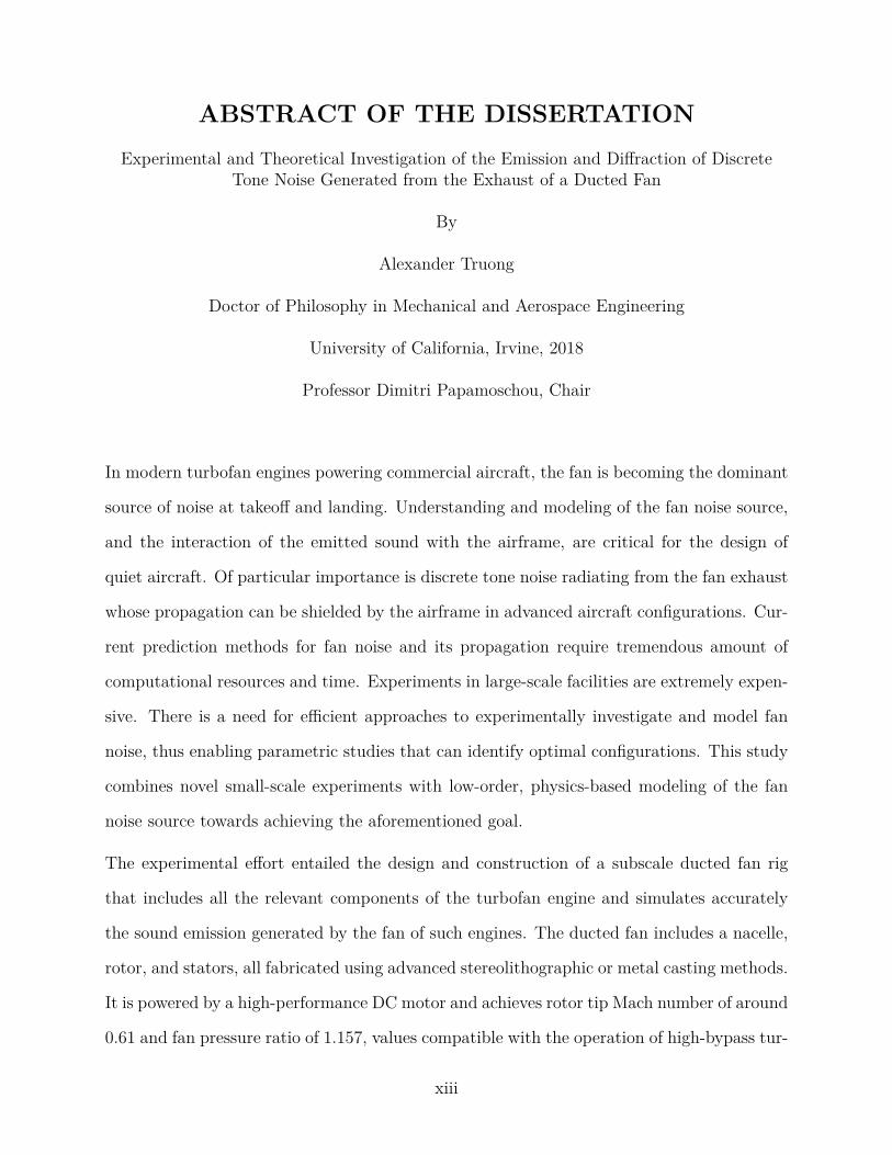
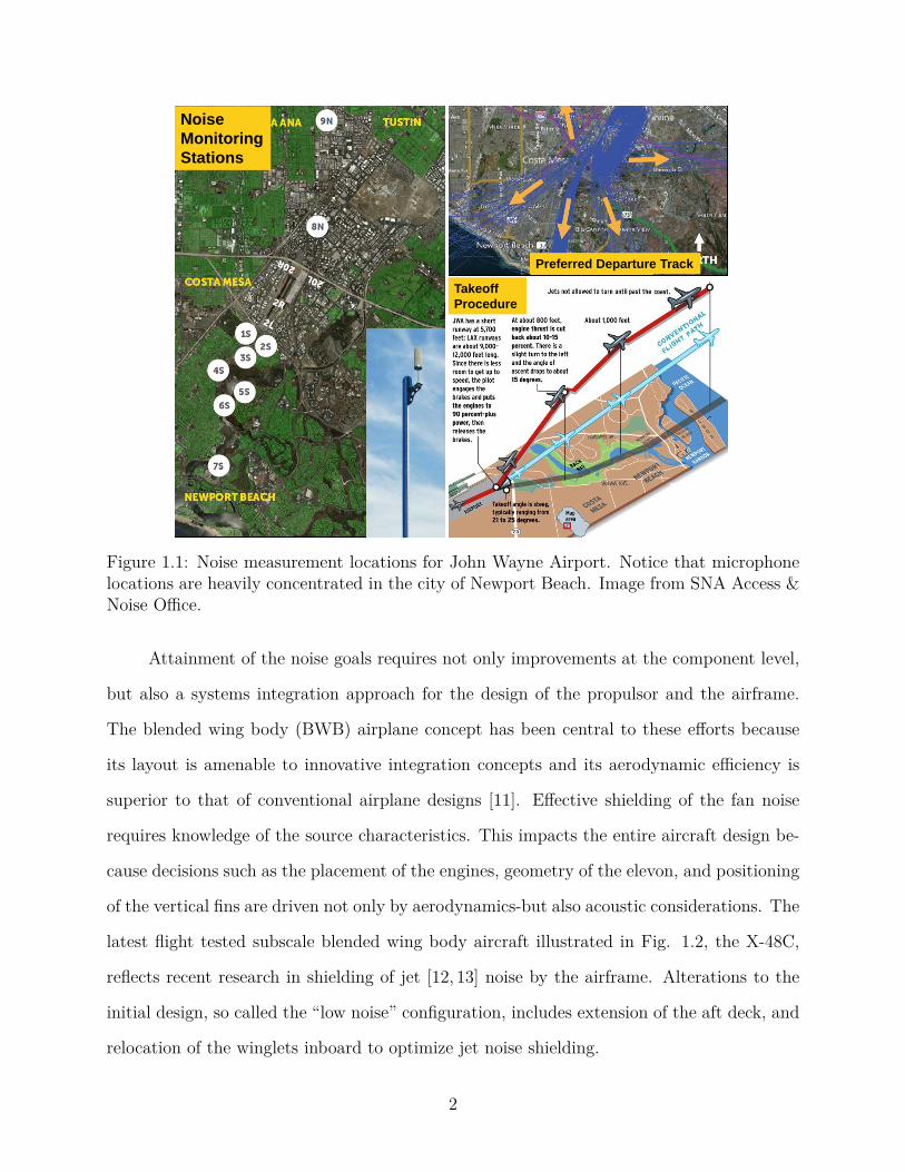
1.1 Noise measurement locations for John Wayne Airport. Notice that micro-phone locations are heavily concentrated in the city of Newport Beach. Imagefrom SNA Access & Noise Office. . . . . . . . . . . . . . . . . . . . . . . . . 2
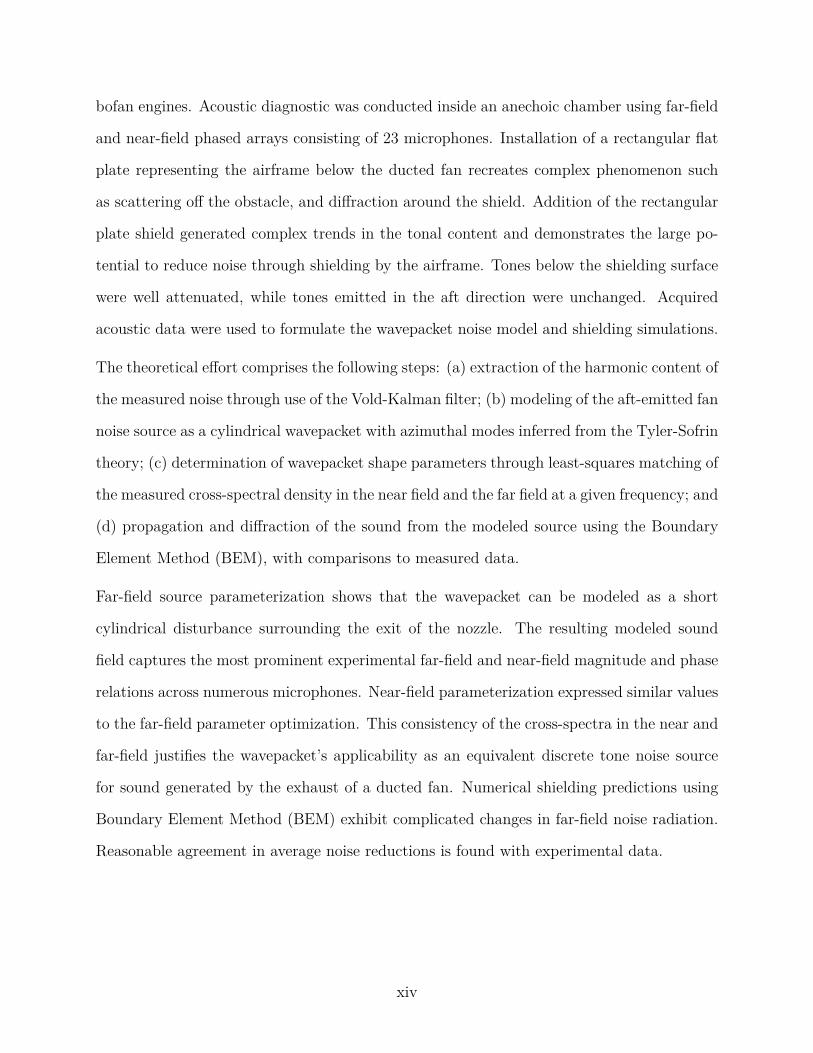
1.2 The X-48C Hybrid Wing Body research aircraft banks right over NASA’sDryden Flight Research Center at Edwards Air Force Base during one of thesub-scale aircraft’s final test flights on Feb. 28, 2013. Credits: NASA CarlaThomas. . . . . . . . . . . . . . . . . . . . . . . . . . . . . . . . . . . . . . . 3
1.3 Boeing Low Speed Aeroacoustics Facility configured for Hybrid Wind Bodyinstallation effects testing from Boeing (left). NASA Langley HWB test sec-tion configuration from NASA George Holmich. . . . . . . . . . . . . . . . . 4
2.1 Organization of literature review chapter. . . . . . . . . . . . . . . . . . . . . 102.2 Display of pressure field components and phase relationship at a fixed instant
of time. . . . . . . . . . . . . . . . . . . . . . . . . . . . . . . . . . . . . . . 112.3 Input pressure distribution and boundary condition of the 3-dimensional wave
guide problem. . . . . . . . . . . . . . . . . . . . . . . . . . . . . . . . . . . 132.4 Surface of constant phase for acoustic transmission through a cylindrical duct
with harmonic forcing. . . . . . . . . . . . . . . . . . . . . . . . . . . . . . . 152.5 Pressure perturbation over a wavy wall for subsonic (left), supersonic (right). 162.6 Pressure perturbation from a wave guide for a subsonic (top), and supersonic
rotor (bottom) for the circumferential and radial mode m = 2, n = 2. Rightimage depicts modal-frequency spectrum of ducted fan noise. . . . . . . . . . 17
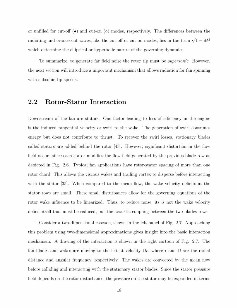
2.7 Depiction of the rotor wakes interaction with the stator (left). Schematic ofrotor wake interaction (right). Image courtesy of Ed Envia of NASA GlennResearch Center [1]. . . . . . . . . . . . . . . . . . . . . . . . . . . . . . . . . 19
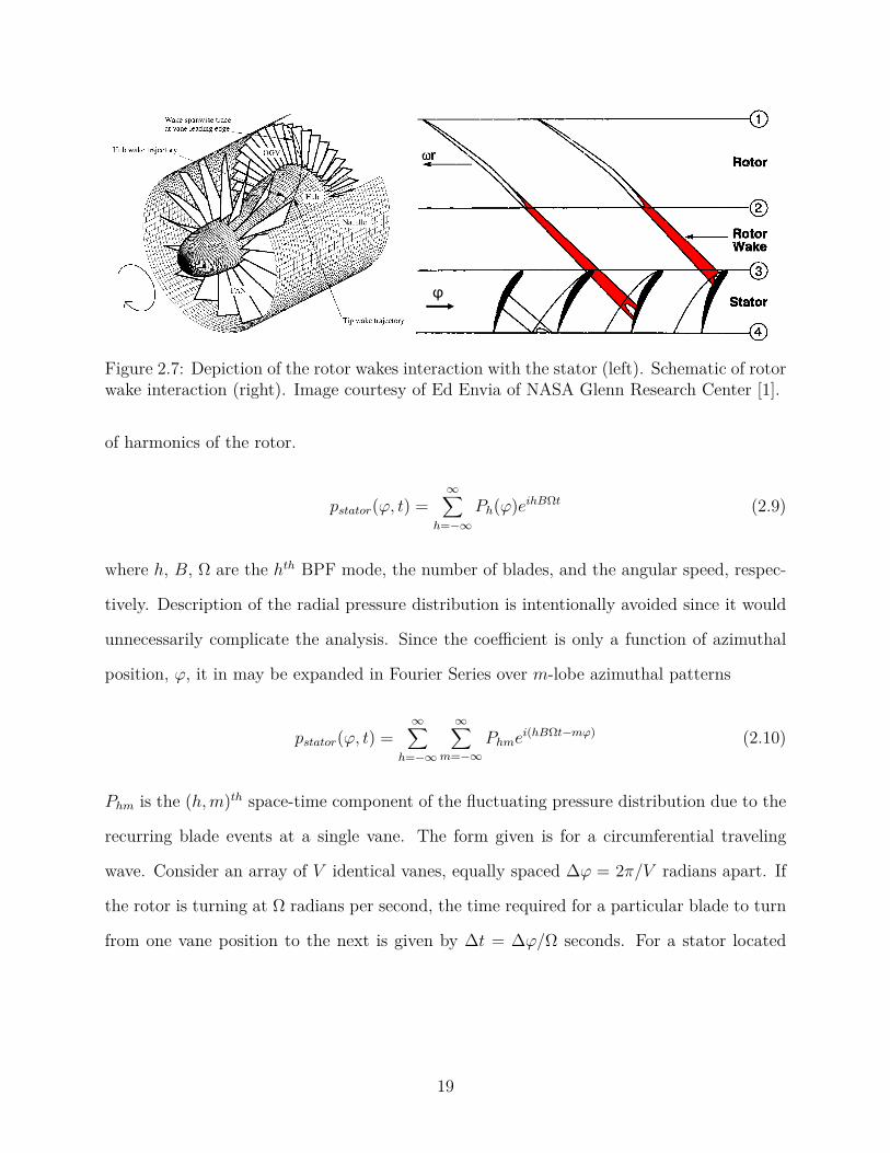
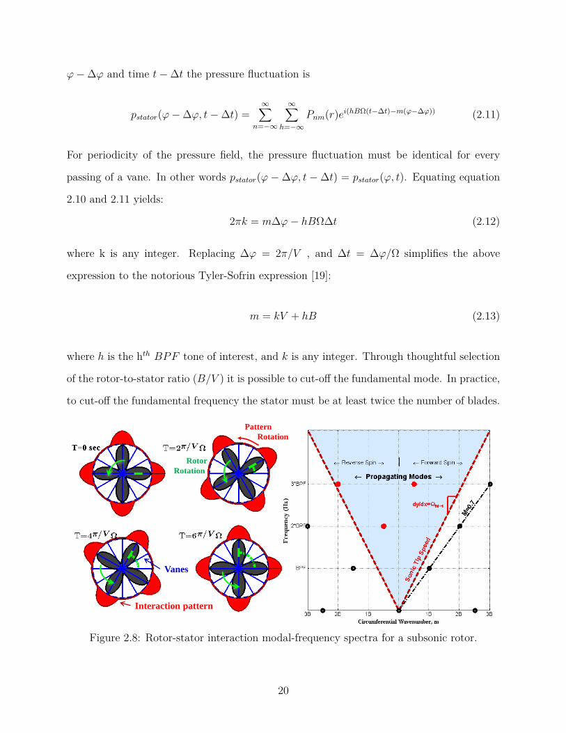
2.8 Rotor-stator interaction modal-frequency spectra for a subsonic rotor. . . . . 202.9 A sketch of the semi-infinite annular duct geometry. . . . . . . . . . . . . . . 222.10 Location of zeros (), and poles (•) of the Wiener-Hopf kernel for annular jet
operating with ω = 4, M2=5, M1 = 0.25, D1 = C1 =1, h=0 . Image fromRienstra [2]. . . . . . . . . . . . . . . . . . . . . . . . . . . . . . . . . . . . . 24
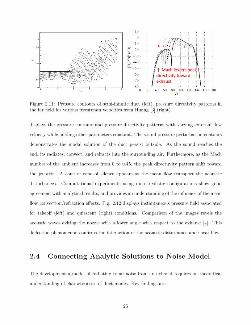
2.11 Pressure contours of semi-infinite duct (left), pressure directivity patterns inthe far field for various freestream velocities from Huang [3] (right). . . . . . 25
2.12 Instantaneous perturbed aft pressure field radiated by the exhaust under take-off M∞ = 0.26, and into a quiescent free stream M∞ = 0 from Redonnet [4]. 26
v
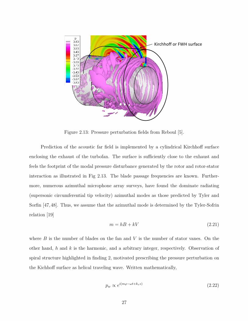
2.13 Pressure perturbation fields from Reboul [5]. . . . . . . . . . . . . . . . . . . 27
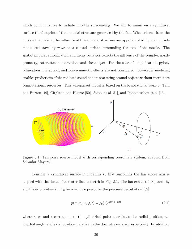
3.1 Fan noise source model with corresponding coordinate system, adapted fromSalvador Mayoral. . . . . . . . . . . . . . . . . . . . . . . . . . . . . . . . . . 30
3.2 Graph of the Hankel function of the first and second kind in the complex plane. 323.3 Flowchart for calculation of near-field pressure. . . . . . . . . . . . . . . . . . 343.4 Schematic of cross-spectra between two microphones. . . . . . . . . . . . . . 363.5 Source Parameterization Procedure . . . . . . . . . . . . . . . . . . . . . . . 383.6 Setup of wavepacket as a radiating body with a boundary . . . . . . . . . . . 403.7 Program layout of wavepacket optimization routine . . . . . . . . . . . . . . 43
4.1 Stations locations of a ducted fan. . . . . . . . . . . . . . . . . . . . . . . . . 454.2 Vector diagram and blade profiles at hub, meanline, and tip. The axial veloc-
ity, cz is independent of radius. Figure adapted from Mechanics and Thermo-dynamics of Propulsion (pg. 334). . . . . . . . . . . . . . . . . . . . . . . . . 46
4.3 Fluent CFD simulation of the rotor blade row. . . . . . . . . . . . . . . . . . 474.4 Overview of the ducted fan design. a) cross-sectional view; b) picture of the
3D printed rotor. . . . . . . . . . . . . . . . . . . . . . . . . . . . . . . . . . 484.5 Principal power components and their installation. . . . . . . . . . . . . . . 494.6 Schematic (left) and picture (right) of airframe shielding rig with insert-able
strips for lengthening of the chord. . . . . . . . . . . . . . . . . . . . . . . . 504.7 Schematic of anechoic chamber and microphone array (left). Picture inside
anechoic showing downward arm holding 24 microphones (right). . . . . . . . 514.8 Installation of fully extended (addition of all strips) shielding surface in ane-
choic chamber (left). Attachment of nearfield microphone array to fan rig(right). . . . . . . . . . . . . . . . . . . . . . . . . . . . . . . . . . . . . . . . 52
4.9 Frame grab of video of flow visualization using smoke and a HeNe laser sheetfor illumination. . . . . . . . . . . . . . . . . . . . . . . . . . . . . . . . . . . 53
4.10 Flowchart of RPM measurement and phasor frequency determination process. 544.11 Frequency time trace during a typical test run (262144 samples). The red
line represents the low-pass filtered component of the RPM sensor output.Rotor speed indicates an average RPM near 57,000 (13.33 kHz) The rotorslows down slightly during the experiment. . . . . . . . . . . . . . . . . . . . 55
4.12 Vold Kalman filter transfer function for various pole counts. . . . . . . . . . 604.13 The Hilbert transform in complex space-time. The analytic signal in complex
space is projected onto the real axis to form the signal. Projection onto theimaginary axis (quadrature) shifts the phase of the real signal by 90. Thiscomplex signal can be written as a complex phasor with amplitude and phase:a(t)ei2πft. . . . . . . . . . . . . . . . . . . . . . . . . . . . . . . . . . . . . . 61
4.14 Oscillator system response in the (y,y,t) space. Projecting the trajectory ontothe displacement time axis gives the measured signal. Mapping the curve tospace and velocity gives the phase portrait. . . . . . . . . . . . . . . . . . . . 62
5.1 Time domain signal decomposition of the ducted fan noise at various polarangles. Total signal (red), broadband (blue), harmonic (black). . . . . . . . . 66
vi
5.2 Narrowband SPL spectra at two polar angles. Total signal (top), harmonic(middle), broadband (bottom). . . . . . . . . . . . . . . . . . . . . . . . . . 67
5.3 Contour plots of narrowband SPL spectra. . . . . . . . . . . . . . . . . . . . 685.4 Effect of shield on acoustics. . . . . . . . . . . . . . . . . . . . . . . . . . . . 705.5 Effect of shield on acoustic directivity of the BPF tones. . . . . . . . . . . . 715.6 Comparison of UCI and NASA Narrowband SPL from Shah [6] for a exhaust
arc microphone at θ = 65.5. . . . . . . . . . . . . . . . . . . . . . . . . . . . 725.7 Comparison of UCI and NASA one-third octave band directivities. Total
signal (red), broadband (blue), harmonic (black). . . . . . . . . . . . . . . . 745.8 Results of parameterization for fundamental blade passage frequency (1 ×
BPF). Plotted is the wavepacket shape. Optimum parameters are ε = 291.8,kz = 169.05 (Uc = 490 m/s), b1/D0 =0.13, b2/D0 =0.70, z0/D0 =0.21. . . . 75
5.9 Results of parameterization for fundamental blade passage frequency (1 ×BPF) in the far-field. Plotted are the modeled (blue) and experimental(black)auto and cross-spectra, and a sketch of the microphone layout. . . . . . . . 76
5.10 Results of parameterization for 2nd harmonic (2 × BPF). Plotted is thewavepacket shape. Optimum parameters are ε = 292.0, kz = 312.57 (Uc =530.68 m/s), b1/D0 =0.10, b2/D0 =0.50, z0/D0 =0.12. . . . . . . . . . . . . 78
5.11 Results of parameterization for fundamental blade passage frequency (2 ×BPF) in the far-field. Plotted are the modeled (blue) and experimental (black)auto and cross-spectra, and a sketch of the microphone layout. . . . . . . . 78
5.12 Results of parameterization for the fundamental blade passage frequency (1 ×BPF) in the near-field. Plotted are the near field parameterized model (blue),far field parameterized model (red), and experimental (black) auto and cross-spectra. The near-field microphone layout is sketched in the lower left corner.. . . . . . . . . . . . . . . . . . . . . . . . . . . . . . . . . . . . . . . . . . . 79
5.13 Rectangular flat plate mesh used in boundary element method (BEM) compu-tations. Red dots in the right image represents the source centers for varioustrailing edge locations, XTE. . . . . . . . . . . . . . . . . . . . . . . . . . . . 81
5.14 Comparison of 1× BPF aft fan noise shielding intensity distributions for ex-perimental investigations and BEM predictions. . . . . . . . . . . . . . . . . 82
6.1 Noise reduction concepts (a) Serrated rotor blade from Gliebe [7], and geom-etry and definition of stator vane: (b) sweep angle and (c) lean angle formEnvia [1]. . . . . . . . . . . . . . . . . . . . . . . . . . . . . . . . . . . . . . 88
vii

LIST OF TABLES
Page
4.1 Design Point Specifications . . . . . . . . . . . . . . . . . . . . . . . . . . . 454.2 Rectangular Shield Specifications . . . . . . . . . . . . . . . . . . . . . . . . 504.3 Filter Comparison . . . . . . . . . . . . . . . . . . . . . . . . . . . . . . . . 64
5.1 Test Matrix for Rectangular Shielded Experiments . . . . . . . . . . . . . . . 695.2 Summary of Fan Specifications and Experimental Conditions . . . . . . . . 725.3 Dominant Azimuthal Modes from Tyler-Sofrin Rule . . . . . . . . . . . . . . 755.4 Far and Near-Field Parameterized Wavepacket Variables . . . . . . . . . . . 805.5 Surface Dimensions and Noise Source Location . . . . . . . . . . . . . . . . . 825.6 Computational and Experimental Shielding Insertion Loss . . . . . . . . . . 83
viii

NOMENCLATURE
AbbreviationsANOPP Aircraft Noise Prediction ProgramBEC Battery Eliminator CircuitBEM Boundary Element MethodBPF Blade Passage FrequencyBWB Blended Wing BodyCAD Computer-Aided DesignCFD Computational Fluid DynamicsDC Direct CurrentFPR Fan Pressure RatioEPNL Effective Perceived Noise LevelESC Electronic Speed ControlFAA Federal Aviation AdministrationFAR Federal Aviation RegulationFFT Fast Fourier TransformFW-H Ffowcs-Williams and HawkingGRC Glenn Research CenterLiPo Lithium-ion Polymer BatteryNASA National Aeronautics and Space AdministrationOASPL Overall Sound Pressure LevelPWM Pulse Width ModulationRANS Reynolds Average Navier-StokesRC Radio ControlRPM Revolution Per MinuteSDT Source Diagnostic TestSLA Sterolithography ApparatusSNA John Wayne Airport, Orange CountySPL Sound Pressure LevelUCI University of California, IrvineVK Vold-KalmanRoman Symbolsa Speed of soundA Structural equation matrixAk Wavepacket parameter vectorb Asymmetric Gaussian widthB Blade countc Chord length of wingcgroup Group velocity: speed at which envelope propagate through spaceC Flow velocity in the absolute frame of reference
ix
Ck Complex phasor matrixCu Absolute tangential velocityCz Axial component of velocitydB DecibelD0 Nozzle exit diameterf Frequencyf(t) Instantaneous frequencyF Fourier TransformG 3D free-space Green’s functionh Harmonic numberH(1)m (z) Hankel function of the first kind of order m, H(1)
m (z) = Jm(z) + iYm(z)H(2)m (z) Hankel function of the second kind of order m, H(2)
m (z) = Jm(z)− iYm(z)Hz Hertzi imaginary unit =
√−1
I Identity matrixJ(x) Cost functionJm(z) Bessel Function of the first kind of order mk Wavenumber or integer in Tyler-Sofrin Rulek0 Acoustic wavenumber, k0 = ω/a∞kr Radial wavenumberkz Axial wavenumberM Mach numberm Azimuthal mode numberm Mass flow ratep Acoustic pressureP Spatial Fourier transform of acoustic pressureP Frequency/Wavenumber Fourier Transform of Pressurep0(z) Wavepacket envelopeP0 Total pressurer Weighting factor in VK filter or radial positionr0 Radius of cylindrical surface on which wavepacket is prescribed onS Wingspant Timet/c Airfoil thickness to chord ratio in percentT0 Total temperatureU VelocityV Vane countvp Phase velocity: rate at which the phase of the wave propagates in spaceW Flow velocity in the relative frame of referenceW (z) Faddeva functionWu Relative tangential velocityx, y, z Cartesian coordinate system positionxk(t) Time-varying (complex) envelope of order ky(t) Total measured acoustic signalYm(z) Bessel Function of the second kind of order mz0 Peak noise location of wavepacket relative to nozzle exit
x
Greek Symbolsα Flow angle in the absolute frame of reference as measured from the axial directionβ Flow angle in the relative frame of reference as measured from the axial directionδ Delta function∆ϕ Angle between stator blades∆t Time for rotor blade to rotate between stator bladesε(t) Error in structural equation fitη(t) Broadband or shaft-uncorrelated noiseη(z) Radial displacement of the vortex sheetθ Polar angle relative to downstream axis (degrees)λ Wavelengthµmn Separation eigenvalue constant for m harmonic and nth zero crossingπ Mathematical constant, π = 3.14159..ρ Densityφ Velocity potentialϕ Azimuthal angleω0 Angular acoustic frequencyΩ Shaft angular frequency (rad/s)∇pxk[n] Structural equation of order p∇2 Laplace operator() Round brackets denote continuous signals[] Square brackets denote discrete signalsSubscripts and Superscriptsexit exit of nozzleexp experimentfar far-fieldH Hermitiani incidentk harmonic or order of signalmax maximum valuemodel modeledm reference microphone number for cross-spectra or azimuthal mode numberstator statorT TransposeTE Trailing edgez Axial∞ Ambient or freestream
xi
CURRICULUM VITAE
Alexander Truong
2018 Ph.D, Mechanical and Aerospace EngineeringUniversity of California, Irvine
2012 Master of Science in Mechanical and Aerospace EngineeringUniversity of California, Irvine
2010 Bachelor of Science in Aerospace EngineeringUniversity of California, Irvine
Publications
Truong, A., and Papamoschou, D.,”Harmonic and Broadband Separation of Noise from aSmall Ducted Fan,” AIAA paper 2015-3282, 21st Aeroacoustics Conference, 22-26 June 2015,Dallas, Texas.
Truong, A., and Papamoschou, D., ”Experimental Simulation of Ducted Fan Acoustics atVery Small Scale,” AIAA paper 2014-0718, 52nd Aerospace Sciences Meeting, 13-17 January2014, National Harbor, Maryland.
Truong, A., and Papamoschou, D., ”Aeroacoustic Testing of Open Rotors at Very SmallScale, ” AIAA paper 2013-0217, 51st Aerospace Sciences Meeting, 07-10 January 2013, Ft.Worth, Texas.
xii
ABSTRACT OF THE DISSERTATIONExperimental and Theoretical Investigation of the Emission and Diffraction of Discrete
Tone Noise Generated from the Exhaust of a Ducted Fan
By
Alexander Truong
Doctor of Philosophy in Mechanical and Aerospace Engineering
University of California, Irvine, 2018
Professor Dimitri Papamoschou, Chair
In modern turbofan engines powering commercial aircraft, the fan is becoming the dominant
source of noise at takeoff and landing. Understanding and modeling of the fan noise source,
and the interaction of the emitted sound with the airframe, are critical for the design of
quiet aircraft. Of particular importance is discrete tone noise radiating from the fan exhaust
whose propagation can be shielded by the airframe in advanced aircraft configurations. Cur-
rent prediction methods for fan noise and its propagation require tremendous amount of
computational resources and time. Experiments in large-scale facilities are extremely expen-
sive. There is a need for efficient approaches to experimentally investigate and model fan
noise, thus enabling parametric studies that can identify optimal configurations. This study
combines novel small-scale experiments with low-order, physics-based modeling of the fan
noise source towards achieving the aforementioned goal.
The experimental effort entailed the design and construction of a subscale ducted fan rig
that includes all the relevant components of the turbofan engine and simulates accurately
the sound emission generated by the fan of such engines. The ducted fan includes a nacelle,
rotor, and stators, all fabricated using advanced stereolithographic or metal casting methods.
It is powered by a high-performance DC motor and achieves rotor tip Mach number of around
0.61 and fan pressure ratio of 1.157, values compatible with the operation of high-bypass tur-
xiii
bofan engines. Acoustic diagnostic was conducted inside an anechoic chamber using far-field
and near-field phased arrays consisting of 23 microphones. Installation of a rectangular flat
plate representing the airframe below the ducted fan recreates complex phenomenon such
as scattering off the obstacle, and diffraction around the shield. Addition of the rectangular
plate shield generated complex trends in the tonal content and demonstrates the large po-
tential to reduce noise through shielding by the airframe. Tones below the shielding surface
were well attenuated, while tones emitted in the aft direction were unchanged. Acquired
acoustic data were used to formulate the wavepacket noise model and shielding simulations.
The theoretical effort comprises the following steps: (a) extraction of the harmonic content of
the measured noise through use of the Vold-Kalman filter; (b) modeling of the aft-emitted fan
noise source as a cylindrical wavepacket with azimuthal modes inferred from the Tyler-Sofrin
theory; (c) determination of wavepacket shape parameters through least-squares matching of
the measured cross-spectral density in the near field and the far field at a given frequency; and
(d) propagation and diffraction of the sound from the modeled source using the Boundary
Element Method (BEM), with comparisons to measured data.
Far-field source parameterization shows that the wavepacket can be modeled as a short
cylindrical disturbance surrounding the exit of the nozzle. The resulting modeled sound
field captures the most prominent experimental far-field and near-field magnitude and phase
relations across numerous microphones. Near-field parameterization expressed similar values
to the far-field parameter optimization. This consistency of the cross-spectra in the near and
far-field justifies the wavepacket’s applicability as an equivalent discrete tone noise source
for sound generated by the exhaust of a ducted fan. Numerical shielding predictions using
Boundary Element Method (BEM) exhibit complicated changes in far-field noise radiation.
Reasonable agreement in average noise reductions is found with experimental data.
xiv

1
Cha
pter
Background and Motivation
It has been over 50 years since the Boeing 707 ushered in both the jet age and the era
of federal mandates requiring minimum noise standards for aircraft entering service.
Takeoff and landing noise in the immediate vicinity of an airport is regulated, cruise is
not. Lack of visible noise abatement technology has been a recognized barrier to unhindered
airport operations. Airports such as JohnWayne in Orange County, California (SNA) enforce
some of the most stringent noise regulations in the United States. Orginally founded as a
rural flight school, the orginal landing strip once surronded by celery fields is now surronded
by permanent noise monitoring stations dispersed amidst suburbia, as portrayed in Fig. 1.1.
For every decibel over the noise limit, approximately twenty passengers must be offloaded
to get inside the limit [8]. Aircraft incapable of meeting noise limitations are not permitted
to land, take-off, or be based at the airport. Such trade-offs and financial liabilities have
motivated considerable research effort in the past to suppress jet noise and understand the
physical process of sound generation of the jet [9]. However, jet noise is no longer the
dominant noise source in modern turbofan powered commercial aircraft [10]. With every
new set of regulations, the airline industry requires upgrades to its jet aircraft, if not new
designs. The combined reality of continued growth in air traffic, increasingly more stringent
environmental goals, and the supplementary limitations imposed by airports- such as curfews,
still results in continued strong demand for aircraft noise reduction technology.
1
Noise
Monitoring
Stations
Takeoff
Procedure
Preferred Departure Track
Figure 1.1: Noise measurement locations for John Wayne Airport. Notice that microphonelocations are heavily concentrated in the city of Newport Beach. Image from SNA Access &Noise Office.
Attainment of the noise goals requires not only improvements at the component level,
but also a systems integration approach for the design of the propulsor and the airframe.
The blended wing body (BWB) airplane concept has been central to these efforts because
its layout is amenable to innovative integration concepts and its aerodynamic efficiency is
superior to that of conventional airplane designs [11]. Effective shielding of the fan noise
requires knowledge of the source characteristics. This impacts the entire aircraft design be-
cause decisions such as the placement of the engines, geometry of the elevon, and positioning
of the vertical fins are driven not only by aerodynamics-but also acoustic considerations. The
latest flight tested subscale blended wing body aircraft illustrated in Fig. 1.2, the X-48C,
reflects recent research in shielding of jet [12, 13] noise by the airframe. Alterations to the
initial design, so called the “low noise” configuration, includes extension of the aft deck, and
relocation of the winglets inboard to optimize jet noise shielding.
2
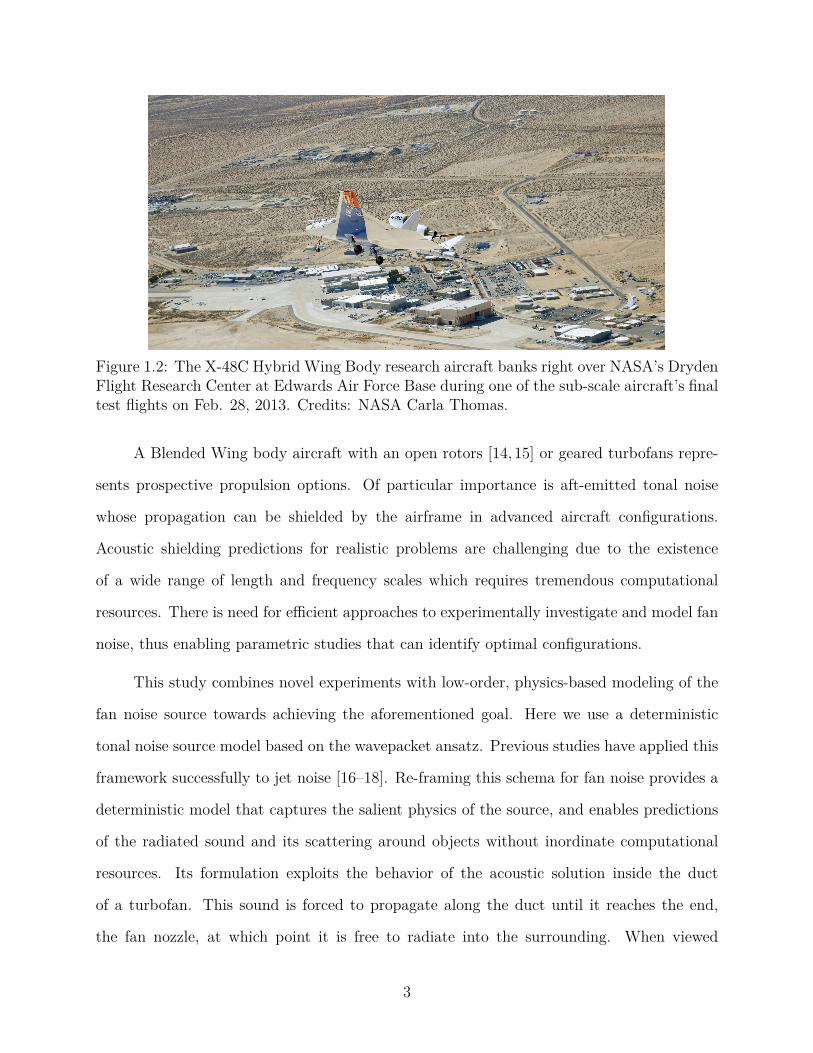
Figure 1.2: The X-48C Hybrid Wing Body research aircraft banks right over NASA’s DrydenFlight Research Center at Edwards Air Force Base during one of the sub-scale aircraft’s finaltest flights on Feb. 28, 2013. Credits: NASA Carla Thomas.
A Blended Wing body aircraft with an open rotors [14, 15] or geared turbofans repre-
sents prospective propulsion options. Of particular importance is aft-emitted tonal noise
whose propagation can be shielded by the airframe in advanced aircraft configurations.
Acoustic shielding predictions for realistic problems are challenging due to the existence
of a wide range of length and frequency scales which requires tremendous computational
resources. There is need for efficient approaches to experimentally investigate and model fan
noise, thus enabling parametric studies that can identify optimal configurations.
This study combines novel experiments with low-order, physics-based modeling of the
fan noise source towards achieving the aforementioned goal. Here we use a deterministic
tonal noise source model based on the wavepacket ansatz. Previous studies have applied this
framework successfully to jet noise [16–18]. Re-framing this schema for fan noise provides a
deterministic model that captures the salient physics of the source, and enables predictions
of the radiated sound and its scattering around objects without inordinate computational
resources. Its formulation exploits the behavior of the acoustic solution inside the duct
of a turbofan. This sound is forced to propagate along the duct until it reaches the end,
the fan nozzle, at which point it is free to radiate into the surrounding. When viewed
3
from the outside the nacelle, the footprint of these modal structures is approximated as a
amplitude modulated traveling wave on a imaginary control surface surrounding the exit of
the nozzle. The fan noise source model shape are described by parameters and azimuthal
modes inferred from Tyler and Sofrin’s rule [19, 20]. The superposition of wavepackets at
various BPF frequencies will reproduce the far-field sound intensity distribution.
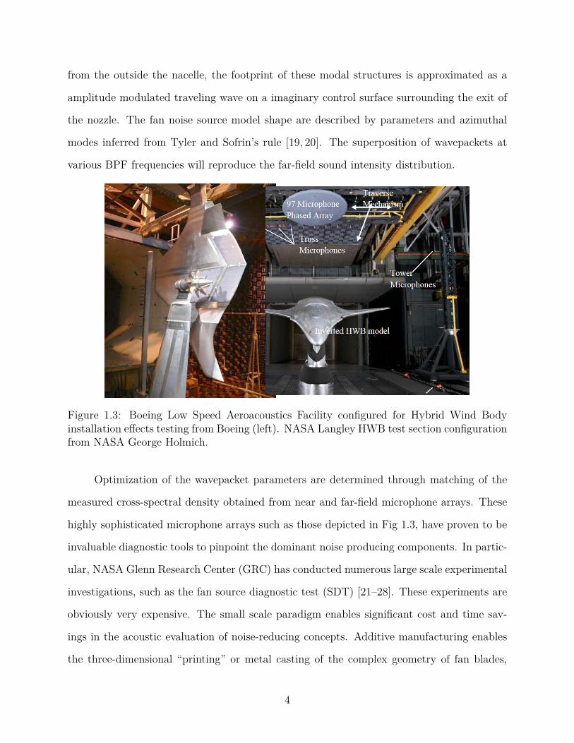
Figure 1.3: Boeing Low Speed Aeroacoustics Facility configured for Hybrid Wind Bodyinstallation effects testing from Boeing (left). NASA Langley HWB test section configurationfrom NASA George Holmich.
Optimization of the wavepacket parameters are determined through matching of the
measured cross-spectral density obtained from near and far-field microphone arrays. These
highly sophisticated microphone arrays such as those depicted in Fig 1.3, have proven to be
invaluable diagnostic tools to pinpoint the dominant noise producing components. In partic-
ular, NASA Glenn Research Center (GRC) has conducted numerous large scale experimental
investigations, such as the fan source diagnostic test (SDT) [21–28]. These experiments are
obviously very expensive. The small scale paradigm enables significant cost and time sav-
ings in the acoustic evaluation of noise-reducing concepts. Additive manufacturing enables
the three-dimensional “printing” or metal casting of the complex geometry of fan blades,
4
and the nacelle structure that are nearly impossible to fabricate using conventional machin-
ing. The rapid-prototyping approach has been used successfully with jet noise testing of
realistic nozzle configurations and open-rotor spinning at full-scale tip speed powered by
high-performance DC motors [12, 15]. More recently, assessments of the relevance of UCI’s
small scale ducted fan indicate that small-scale models reproduce with good fidelity the main
acoustic features [29] . This simulator generates tonal, broadband, and jet noise components
simultaneously.
Noise assessment requires the determination of the tonal and broadband components to
properly assess the efficacy of noise mitigation strategies and for validating prediction codes.
Fan harmonic components occurs at integer multiples of the fundamental frequency (the so-
called orders), i.e., engine rotational speed. On the other hand, broadband noise is random
in nature and is generated from an array of source mechanisms such as turbulence interaction
noise, rotor-stator interaction noise, and trailing edge noise [8]. Each noise component, tonal
or broadband, can have different directivity. The level of shielding will depend not only on the
source location, but also the directivity and radiation patterns. Thus, knowledge of the tonal
and broadband noise content is essential for predicting and optimizing propulsion-airframe
integration. Even when tones strongly protrude from the background, the decomposition of
the tonal and broadband noise components establishes the importance of broadband noise
[30].
Since propulsion noise sources have different characteristics, thus different acoustic
propagation effects, the data must be decomposed into its tonal and broadband components.
Tonal isolation techniques include the peak-finding algorithm, moving medium curve, phase
averaging, and Sree’s Method [14,30–32]. However, frequency domain methods cannot easily
localize information in the time domain, nor compensate for fluctuations intrinsic to real
world experiments. A recent NASA SDT investigation employed a Vold-Kalman (VK) signal
processing technique to filter out the harmonic noise sources [6,33]. This tool performs a time-
domain decomposition of a measured signal into phase-accurate time history of fan harmonic
5
and broadband constituents. The output from the filter has a much higher resolution and
dynamic range than a Fast Fourier Transform (FFT) or phase averaging procedure. In a
similar fashion, this study applies the Vold-Kalman order tracking to acoustics measurements
of a small ducted fan.
The experimental effort entailed the design and construction of a small-scaled ducted
fan rig that includes all the relevant components of the turbofan engine and simulates ac-
curately the sound emission generated by the fan of such engines. The ducted fan includes
a nacelle, rotor, and stators, all fabricated using advanced stereolithographic methods. It
is powered by a high performance brushless motor and achieves rotor tip Mach number of
around 0.61 and fan pressure ratio of 1.157, values comparable with operation of high-bypass
turbofan engines. This one-of-a-kind experimental rig produces radiation patterns compara-
ble with those measured in large-scale NASA experiments at similar conditions. Installation
of a surface representing the airframe enables experimental studies on the diffraction of the
sound generated by a ducted fan.
The theoretical effort comprises the following steps: (a) extraction of the harmonic
content of the measured noise through use of the Vold-Kalman filter; (b) modeling of the
aft-emitted fan noise source as a cylindrical wavepacket with azimuthal modes inferred from
the Tyler-Sofrin theory; (c) determination of wavepacket shape parameters through least-
squares matching of the measured cross-spectral density in the near and far field at a given
frequency; and (d) propagation and diffraction of the sound from the modeled source using
the Boundary Element Method (BEM), with comparisons to measured data. The intent is to
develop predictive methodologies that will be integrated in the next generation Aircraft Noise
Prediction Program (ANOPP) tool to provide better prediction of future aircraft technology.
Thus, we aim to provide the capability and framework to integrate acoustic approaches for
aircraft noise component prediction, and quantifying propulsion system installation effects.
This new framework provides more general methods for the effects related to propulsion
airframe aeroacoustic interaction, and allows for low-noise optimization of the BWB aircraft
6
with geared turbofans. In addition, such improvements strengthen insight and understanding
into controlling noise physics.
1.1 Objectives
The major goals of the study are:
• Development of small-scale ducted fan with realistic noise emission pattern.
• Acoustic far-field and near-field phased array investigation of the sound generated from
the exhaust of a ducted fan.
• Extraction of tonal and broadband components from a small-scale simulator that cap-
tures the physics of fan noise generation using a Vold-Kalman filter.
• Development of a novel exhaust fan noise source model based on the wavepacket ansatz
that captures the salient physics of the source and reproduces faithfully the acoustic
field.
• Source parameterization and application of minimization methods to match the cross-
spectral density of the near and far-field sound at a given BPF frequency.
• Computation of the scattered acoustic field from the wavepacket noise source model
using boundary element method (BEM).
1.2 Thesis Overview
• Chapter 1 : Discusses the historical background and the objective of the research.
• Chapter 2: Literature review of the concepts and equations vital to the study of
ducted fan noise.
7

• Chapter 3: Wavepacket noise source model, wavepacket shape reconstruction from
experimental data, and numerical scattering predictions.
• Chapter 4: Details the facilities used in the experiments and signal processing tech-
niques.
• Chapter 5: Presents and discusses the acoustic results.
• Chapter 6: Conclusion and future work.
8
2
Cha
pter
Discrete Turbomachinery Noise
Sources
This section introduces the concepts and equations that are central to the study of
discrete turbofan noise. The aim is to understand the characteristics and mechanisms
of aft-emitted tonal sound from a turbofan engine to effectively formulate the noise source
representation. To begin, fan noise is caused by periodic motion of the rotor blades. In
high bypass ratio turbofans, the fan is enclosed within a duct system which contain stators.
This duct confines the propagation of noise downstream until it is radiated from the exhaust
of the ducted fan. Thus, the acoustic system consist of the fan noise source, the duct, the
stators, and the exterior of the engine to which the acoustic field is radiated. It is intuitive
to isolate these constituents. Specifically, the development of concepts is broken down into
four distinct segments. First, the characteristics and mechanism of rotor noise are described,
and then extended to duct transmission. Next, we tackle rotor-stator interaction. Lastly,
the emission from the exhaust of the ducted fan is reviewed. This chapter is based on the
synthesis of literature from Magliozzi and Smith and many others [1, 8, 20, 34–36]. It is
assumed no coupling between other source term exists. This simplification allows the source
contribution of each element to be considered independently and is foundation to many fan
noise models [1, 37]. That is, the coupling between the rotor and stators is only acoustical.
9
These findings enable the development of a physics-based noise source model. Knowledge of
the mode pattern and propagating characteristics will help configure a accurate noise source
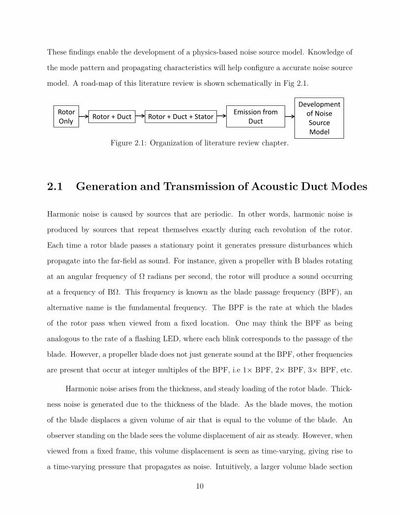
model. A road-map of this literature review is shown schematically in Fig 2.1.
RotorOnly
Rotor + Duct Rotor + Duct + StatorEmission from
Duct
Development of Noise Source Model
Figure 2.1: Organization of literature review chapter.
2.1 Generation and Transmission of Acoustic Duct Modes
Harmonic noise is caused by sources that are periodic. In other words, harmonic noise is
produced by sources that repeat themselves exactly during each revolution of the rotor.
Each time a rotor blade passes a stationary point it generates pressure disturbances which
propagate into the far-field as sound. For instance, given a propeller with B blades rotating
at an angular frequency of Ω radians per second, the rotor will produce a sound occurring
at a frequency of BΩ. This frequency is known as the blade passage frequency (BPF), an
alternative name is the fundamental frequency. The BPF is the rate at which the blades
of the rotor pass when viewed from a fixed location. One may think the BPF as being
analogous to the rate of a flashing LED, where each blink corresponds to the passage of the
blade. However, a propeller blade does not just generate sound at the BPF, other frequencies
are present that occur at integer multiples of the BPF, i.e 1× BPF, 2× BPF, 3× BPF, etc.
Harmonic noise arises from the thickness, and steady loading of the rotor blade. Thick-
ness noise is generated due to the thickness of the blade. As the blade moves, the motion
of the blade displaces a given volume of air that is equal to the volume of the blade. An
observer standing on the blade sees the volume displacement of air as steady. However, when
viewed from a fixed frame, this volume displacement is seen as time-varying, giving rise to
a time-varying pressure that propagates as noise. Intuitively, a larger volume blade section
10
generates more thickness noise. Hence, one should use a thinner section to reduce thickness
noise.
Steady loading noise is the sound that is created by the steady aerodynamic forces
acting on the blade surfaces. In the case of steady loading, the lift and drag on the blade
are constant when the observer is attached to the moving blade. Transformation to a fixed
reference frame, gives a different perspective where the observer sees the direction of the
aerodynamic force vector change in time. This phenomenon gives rise to a time-varying
pressure field that propagates as sound.
T = t0
Fu
nd
am
en
tal
Mo
de
T = t1
T = t2
T = t0
1st
Harm
on
ic
T = t1
T = t2
p
p()
2nd
har
monic
ϕ
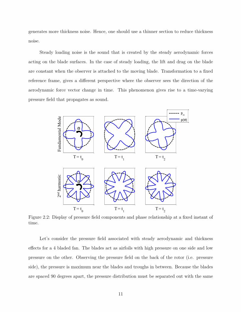
Figure 2.2: Display of pressure field components and phase relationship at a fixed instant oftime.
Let’s consider the pressure field associated with steady aerodynamic and thickness
effects for a 4 bladed fan. The blades act as airfoils with high pressure on one side and low
pressure on the other. Observing the pressure field on the back of the rotor (i.e. pressure
side), the pressure is maximum near the blades and troughs in between. Because the blades
are spaced 90 degrees apart, the pressure distribution must be separated out with the same
11
angular division, as illustrated in the upper left image of Fig 2.2 [38]. As time advances, the
pressure distribution spins with the angular velocity of the fan, Ω with respect to a fixed
observer on the ground. The form of the pressure field, p(ϕ, t) is a spinning wave with 4
lobe pattern rotating at the shaft speed. The spinning pressure patterns generated by the
rotating fan blades are called acoustic modes. The total rotor pressure field consists of a
superposition of lobed patterns all turning with the shaft speed. These pressure pattern are
like spokes on a wheel. The fundamental is associated with a 4 lobe pattern, while the second
harmonic have patterns twice this number of lobes as depicted in the lower panel of Fig 2.2.
The fluctuating pressure field is defined by its circumferential order m, and represented as a
Fourier series specified at some reference plane near the rotor by [39]:
p(r, ϕ, t) =∞∑
m=−∞Fm(r) exp
[i(mBΩt−mBϕ)
](2.1)
Where the F (r) represents the radial distribution, B is the number of blades, and m is the
harmonic.
When the fan is enclosed in a duct, the pressure perturbations must propagate through
the channel before emanating to an observer outside the duct. The dynamics of the propa-
gation are governed by the Naiver-Stokes equations, or the Euler equations- if viscosity can
be neglected. For small disturbances, the governing dynamics are linearized [40]. Reduction
to the canonical wave equation is possible when the flow is uniform (exact) or a potential
(low-Mach number approximation). For a uniform axial flow (~U = Uz + 0er + 0eϕ) the
pressure field satisfies the convective wave equation:
1a2∞
( ∂∂t
+ U∂
∂z)2p = ∇2p
Expand−−−−→ 1a2∞
(∂2p
∂t2+ 2U ∂p
∂t∂z+ U2∂
2p
∂z2 ) = ∇2p (2.2)
where p is the acoustic pressure, and ∇2 is the three-dimensional Laplace operator. A
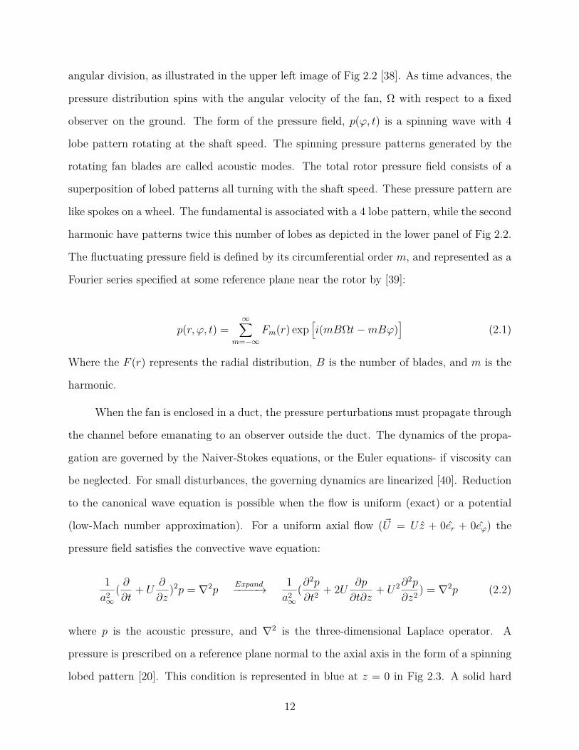
pressure is prescribed on a reference plane normal to the axial axis in the form of a spinning
lobed pattern [20]. This condition is represented in blue at z = 0 in Fig 2.3. A solid hard
12
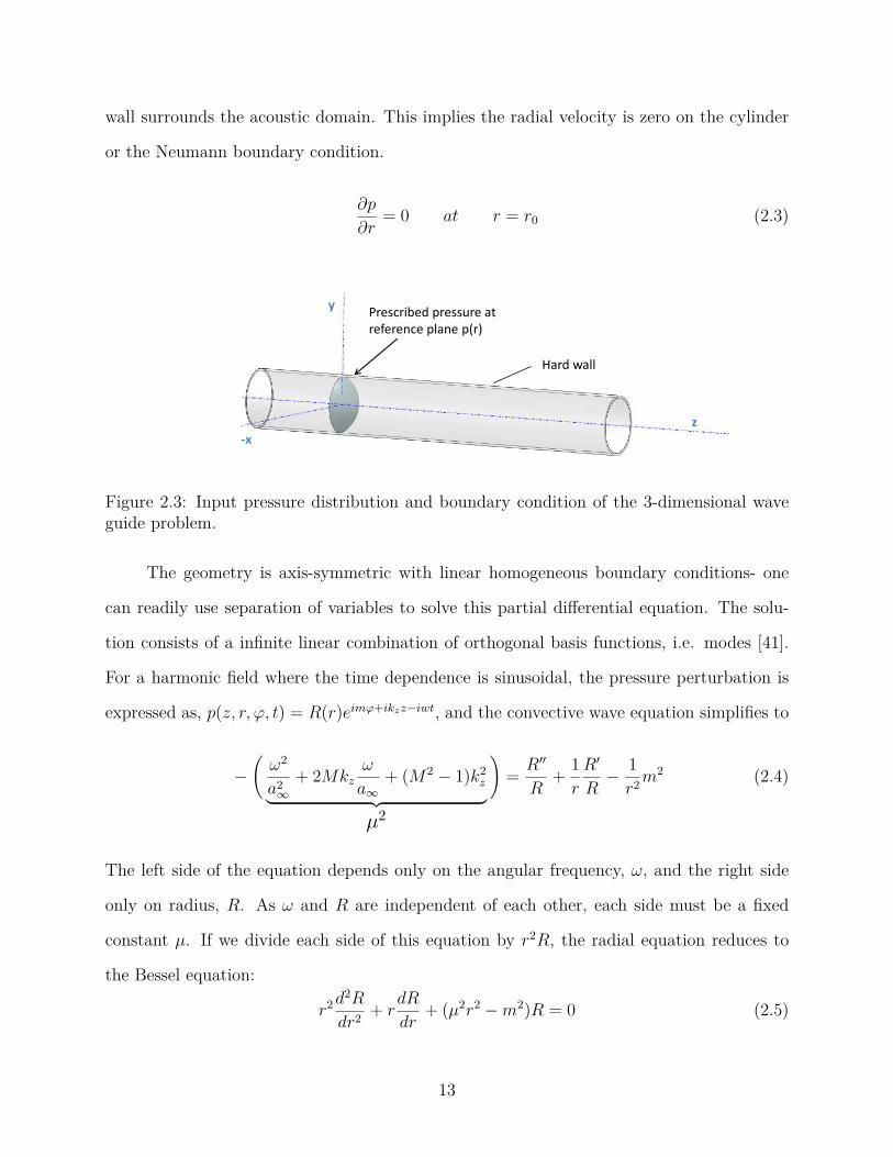
wall surrounds the acoustic domain. This implies the radial velocity is zero on the cylinder
or the Neumann boundary condition.
∂p
∂r= 0 at r = r0 (2.3)
-x
y
z
Hard wall
Prescribed pressure at reference plane p(r)
Figure 2.3: Input pressure distribution and boundary condition of the 3-dimensional waveguide problem.
The geometry is axis-symmetric with linear homogeneous boundary conditions- one
can readily use separation of variables to solve this partial differential equation. The solu-
tion consists of a infinite linear combination of orthogonal basis functions, i.e. modes [41].
For a harmonic field where the time dependence is sinusoidal, the pressure perturbation is
expressed as, p(z, r, ϕ, t) = R(r)eimϕ+ikzz−iwt, and the convective wave equation simplifies to
−(ω2
a2∞
+ 2Mkzω
a∞+ (M2 − 1)k2
z︸ ︷︷ ︸µ2
)= R′′
R+ 1r
R′
R− 1r2m
2 (2.4)
The left side of the equation depends only on the angular frequency, ω, and the right side
only on radius, R. As ω and R are independent of each other, each side must be a fixed
constant µ. If we divide each side of this equation by r2R, the radial equation reduces to
the Bessel equation:
r2d2R
dr2 + rdR
dr+ (µ2r2 −m2)R = 0 (2.5)
13
This well known ODE has a general solution consisting of two linearly independent functions,
Jm(µmnr), Ym(µmnr). Using the boundness condition |R(0)| < ∞, eliminates Ym(r). In
addition, in order for R(r) to be zero on the boundary of the pipe (no-slip), we must pick
the separation constant µ to be one of the roots of J ′m(µr0) = 0. That is, the radial wave
number, kr,mn are the position of the nth zero crossing of the derivative of the Bessel function
of the first kind (d/dzJm(z)) of order m.
µmn = kr,mnr0
(2.6)
These roots are obtained numerically or from tables. Recalling the expression for the separa-
tion constant, µ and denoting the acoustic wave number as k0 = ω/a∞, the axial wavenum-
ber, kz,mn of the (m,n) acoustic mode is given by [42]
k±z,mn =Mk0 ±
√k2
0 − µ2mn(1−M2)
1−M2 = k0
1−M2
[M ±
√√√√1− µ2mn(1−M2)
k20
](2.7)
The above equation gives the axial wavenumber kz in terms of the acoustic wavenumber
k0. This expression is called the dispersion relation. Note that the dispersion equation is
not linear, i.e kz depends on the square of the acoustic wavenumber k0 and the combined
radial-circumferential wave number µmn. Waves with different frequencies have different
phase speeds and as a result the waves disperse as they propagate through the waveguide.
We have just solved the eigenvalue problem. The solution is the product of each spatial
component in the r, ϕ, and z directions. The solution for the acoustic field is:
p(z, r, ϕ, ω) =∞∑
m=−∞
∞∑n=1
A±mnJm(kr,mnr
r0) exp(i[mϕ+ k±z,mnz − ωt]) (2.8)
Three key findings can be inferred from the above expression. Firstly, the acoustic
14
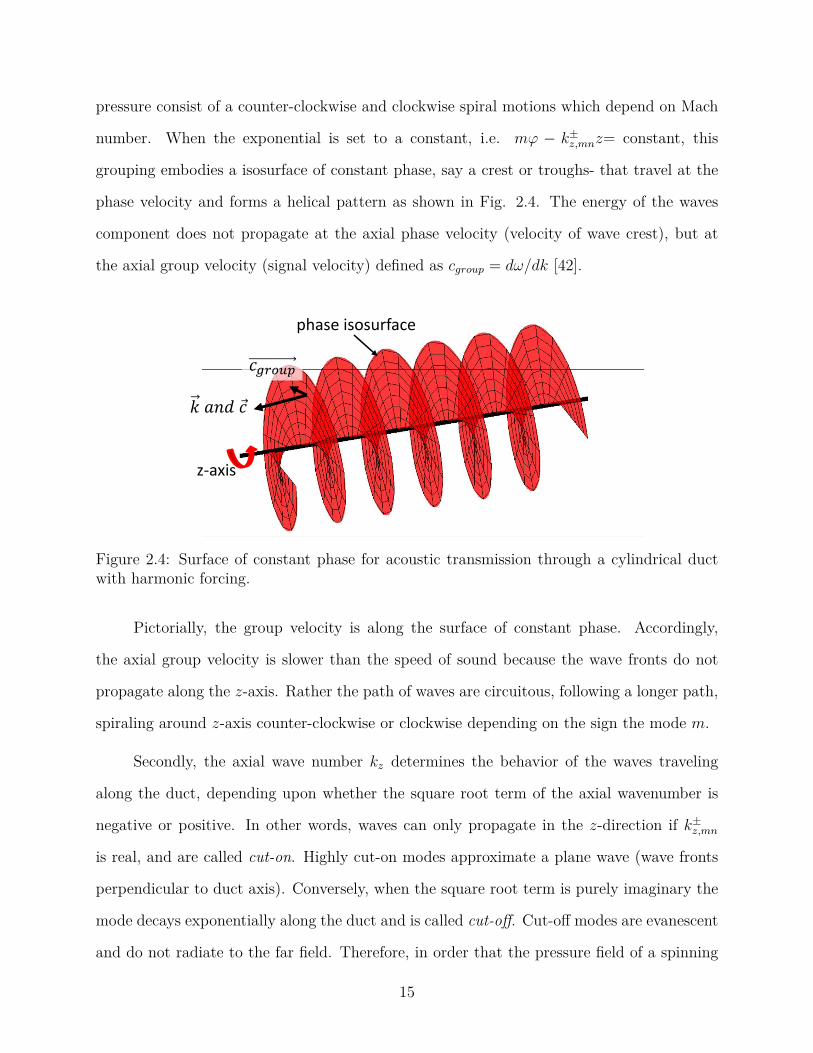
pressure consist of a counter-clockwise and clockwise spiral motions which depend on Mach
number. When the exponential is set to a constant, i.e. mϕ − k±z,mnz= constant, this
grouping embodies a isosurface of constant phase, say a crest or troughs- that travel at the
phase velocity and forms a helical pattern as shown in Fig. 2.4. The energy of the waves
component does not propagate at the axial phase velocity (velocity of wave crest), but at
the axial group velocity (signal velocity) defined as cgroup = dω/dk [42].
z-axis
phase isosurface
𝑘 𝑎𝑛𝑑 Ԧ𝑐
𝑐𝑔𝑟𝑜𝑢𝑝
Figure 2.4: Surface of constant phase for acoustic transmission through a cylindrical ductwith harmonic forcing.
Pictorially, the group velocity is along the surface of constant phase. Accordingly,
the axial group velocity is slower than the speed of sound because the wave fronts do not
propagate along the z-axis. Rather the path of waves are circuitous, following a longer path,
spiraling around z-axis counter-clockwise or clockwise depending on the sign the mode m.
Secondly, the axial wave number kz determines the behavior of the waves traveling
along the duct, depending upon whether the square root term of the axial wavenumber is
negative or positive. In other words, waves can only propagate in the z-direction if k±z,mn
is real, and are called cut-on. Highly cut-on modes approximate a plane wave (wave fronts
perpendicular to duct axis). Conversely, when the square root term is purely imaginary the
mode decays exponentially along the duct and is called cut-off. Cut-off modes are evanescent
and do not radiate to the far field. Therefore, in order that the pressure field of a spinning
15
lobed pattern pattern to propagate, the circumferential Mach number,Mϕ at which it sweeps
the annuls walls, must be supersonic. So, if the helical blade tip Mach number is smaller
than the speed of sound, the rotor does not emit sound into the far field. This quantization
of discrete modes is equivalent to the radiating and evanescent modes of the classical wavy
wall problem.
X/L
Y/L
Pressure contour of M=1.4
0 5 10 15 20 25 30 35 400
5
10
15
20
25
30
35
40
X/L
Y/L
Pressure contour of M=0.6
M
0 5 10 15 20 25 30 35 400
5
10
15
20
25
30
35
40
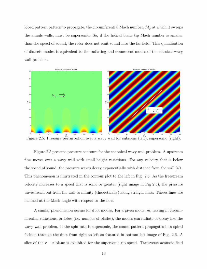
Figure 2.5: Pressure perturbation over a wavy wall for subsonic (left), supersonic (right).
Figure 2.5 presents pressure contours for the canonical wavy wall problem. A upstream
flow moves over a wavy wall with small height variations. For any velocity that is below
the speed of sound, the pressure waves decay exponentially with distance from the wall [40].
This phenomenon is illustrated in the contour plot to the left in Fig. 2.5. As the freestream
velocity increases to a speed that is sonic or greater (right image in Fig 2.5), the pressure
waves reach out from the wall to infinity (theoretically) along straight lines. Theses lines are
inclined at the Mach angle with respect to the flow.
A similar phenomenon occurs for duct modes. For a given mode, m, having m circum-
ferential variations, or lobes (i.e. number of blades), the modes can radiate or decay like the
wavy wall problem. If the spin rate is supersonic, the sound pattern propagates in a spiral
fashion through the duct from right to left as featured in bottom left image of Fig. 2.6. A
slice of the r − z plane is exhibited for the supersonic tip speed. Transverse acoustic field
16
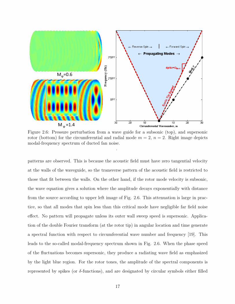
Mϕ=0.6
M ϕ =1.4
Figure 2.6: Pressure perturbation from a wave guide for a subsonic (top), and supersonicrotor (bottom) for the circumferential and radial mode m = 2, n = 2. Right image depictsmodal-frequency spectrum of ducted fan noise.
.
patterns are observed. This is because the acoustic field must have zero tangential velocity
at the walls of the waveguide, so the transverse pattern of the acoustic field is restricted to
those that fit between the walls. On the other hand, if the rotor mode velocity is subsonic,
the wave equation gives a solution where the amplitude decays exponentially with distance
from the source according to upper left image of Fig. 2.6. This attenuation is large in prac-
tice, so that all modes that spin less than this critical mode have negligible far field noise
effect. No pattern will propagate unless its outer wall sweep speed is supersonic. Applica-
tion of the double Fourier transform (at the rotor tip) in angular location and time generate
a spectral function with respect to circumferential wave number and frequency [19]. This
leads to the so-called modal-frequency spectrum shown in Fig. 2.6. When the phase speed
of the fluctuations becomes supersonic, they produce a radiating wave field as emphasized
by the light blue region. For the rotor tones, the amplitude of the spectral components is
represented by spikes (or δ-functions), and are designated by circular symbols either filled
17
or unfilled for cut-off (•) and cut-on () modes, respectively. The differences between the
radiating and evanescent waves, like the cut-off or cut-on modes, lies in the term√
1−M2
which determine the elliptical or hyperbolic nature of the governing dynamics.
To summarize, to generate far field noise the rotor tip must be supersonic. However,
the next section will introduce a important mechanism that allows radiation for fan spinning
with subsonic tip speeds.
2.2 Rotor-Stator Interaction
Downstream of the fan are stators. One factor leading to loss of efficiency in the engine
is the induced tangential velocity or swirl to the wake. The generation of swirl consumes
energy but does not contribute to thrust. To recover the swirl losses, stationary blades
called stators are added behind the rotor [43]. However, significant distortion in the flow
field occurs since each stator modifies the flow field generated by the previous blade row as
depicted in Fig. 2.6. Typical fan applications have rotor-stator spacing of more than one
rotor chord. This allows the viscous wakes and trailing vortex to disperse before interacting
with the stator [35]. When compared to the mean flow, the wake velocity deficits at the
stator rows are small. These small disturbances allow for the governing equations of the
rotor wake influence to be linearized. Thus, to reduce noise, its is not the wake velocity
deficit itself that must be reduced, but the acoustic coupling between the two blades rows.
Consider a two-dimensional cascade, shown in the left panel of Fig. 2.7. Approaching
this problem using two-dimensional approximations gives insight into the basic interaction
mechanism. A drawing of the interaction is shown in the right cartoon of Fig. 2.7. The
fan blades and wakes are moving to the left at velocity Ωr, where r and Ω are the radial
distance and angular frequency, respectively. The wakes are convected by the mean flow
before colliding and interacting with the stationary stator blades. Since the stator pressure
field depends on the rotor disturbance, the pressure on the stator may be expanded in terms
18
ϕ
Figure 2.7: Depiction of the rotor wakes interaction with the stator (left). Schematic of rotorwake interaction (right). Image courtesy of Ed Envia of NASA Glenn Research Center [1].
of harmonics of the rotor.
pstator(ϕ, t) =∞∑
h=−∞Ph(ϕ)eihBΩt (2.9)
where h, B, Ω are the hth BPF mode, the number of blades, and the angular speed, respec-
tively. Description of the radial pressure distribution is intentionally avoided since it would
unnecessarily complicate the analysis. Since the coefficient is only a function of azimuthal
position, ϕ, it in may be expanded in Fourier Series over m-lobe azimuthal patterns
pstator(ϕ, t) =∞∑
h=−∞
∞∑m=−∞
Phmei(hBΩt−mϕ) (2.10)
Phm is the (h,m)th space-time component of the fluctuating pressure distribution due to the
recurring blade events at a single vane. The form given is for a circumferential traveling
wave. Consider an array of V identical vanes, equally spaced ∆ϕ = 2π/V radians apart. If
the rotor is turning at Ω radians per second, the time required for a particular blade to turn
from one vane position to the next is given by ∆t = ∆ϕ/Ω seconds. For a stator located
19
ϕ−∆ϕ and time t−∆t the pressure fluctuation is
pstator(ϕ−∆ϕ, t−∆t) =∞∑
n=−∞
∞∑h=−∞
Pnm(r)ei(hBΩ(t−∆t)−m(ϕ−∆ϕ)) (2.11)
For periodicity of the pressure field, the pressure fluctuation must be identical for every
passing of a vane. In other words pstator(ϕ−∆ϕ, t−∆t) = pstator(ϕ, t). Equating equation
2.10 and 2.11 yields:
2πk = m∆ϕ− hBΩ∆t (2.12)
where k is any integer. Replacing ∆ϕ = 2π/V , and ∆t = ∆ϕ/Ω simplifies the above
expression to the notorious Tyler-Sofrin expression [19]:
m = kV + hB (2.13)
where h is the hth BPF tone of interest, and k is any integer. Through thoughtful selection
of the rotor-to-stator ratio (B/V ) it is possible to cut-off the fundamental mode. In practice,
to cut-off the fundamental frequency the stator must be at least twice the number of blades.
Vanes
Interaction pattern
Pattern
Rotation
Rotor
Rotation
Figure 2.8: Rotor-stator interaction modal-frequency spectra for a subsonic rotor.
20
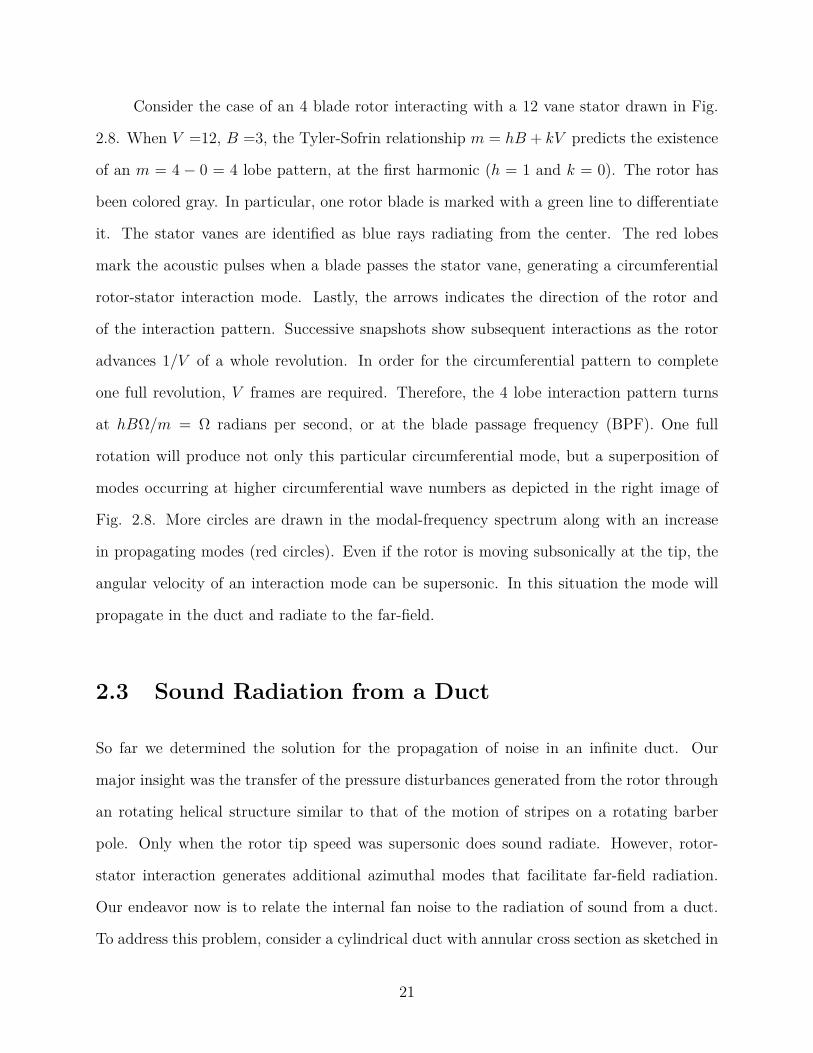
Consider the case of an 4 blade rotor interacting with a 12 vane stator drawn in Fig.
2.8. When V =12, B =3, the Tyler-Sofrin relationship m = hB + kV predicts the existence
of an m = 4 − 0 = 4 lobe pattern, at the first harmonic (h = 1 and k = 0). The rotor has
been colored gray. In particular, one rotor blade is marked with a green line to differentiate
it. The stator vanes are identified as blue rays radiating from the center. The red lobes
mark the acoustic pulses when a blade passes the stator vane, generating a circumferential
rotor-stator interaction mode. Lastly, the arrows indicates the direction of the rotor and
of the interaction pattern. Successive snapshots show subsequent interactions as the rotor
advances 1/V of a whole revolution. In order for the circumferential pattern to complete
one full revolution, V frames are required. Therefore, the 4 lobe interaction pattern turns
at hBΩ/m = Ω radians per second, or at the blade passage frequency (BPF). One full
rotation will produce not only this particular circumferential mode, but a superposition of
modes occurring at higher circumferential wave numbers as depicted in the right image of
Fig. 2.8. More circles are drawn in the modal-frequency spectrum along with an increase
in propagating modes (red circles). Even if the rotor is moving subsonically at the tip, the
angular velocity of an interaction mode can be supersonic. In this situation the mode will
propagate in the duct and radiate to the far-field.
2.3 Sound Radiation from a Duct
So far we determined the solution for the propagation of noise in an infinite duct. Our
major insight was the transfer of the pressure disturbances generated from the rotor through
an rotating helical structure similar to that of the motion of stripes on a rotating barber
pole. Only when the rotor tip speed was supersonic does sound radiate. However, rotor-
stator interaction generates additional azimuthal modes that facilitate far-field radiation.
Our endeavor now is to relate the internal fan noise to the radiation of sound from a duct.
To address this problem, consider a cylindrical duct with annular cross section as sketched in
21
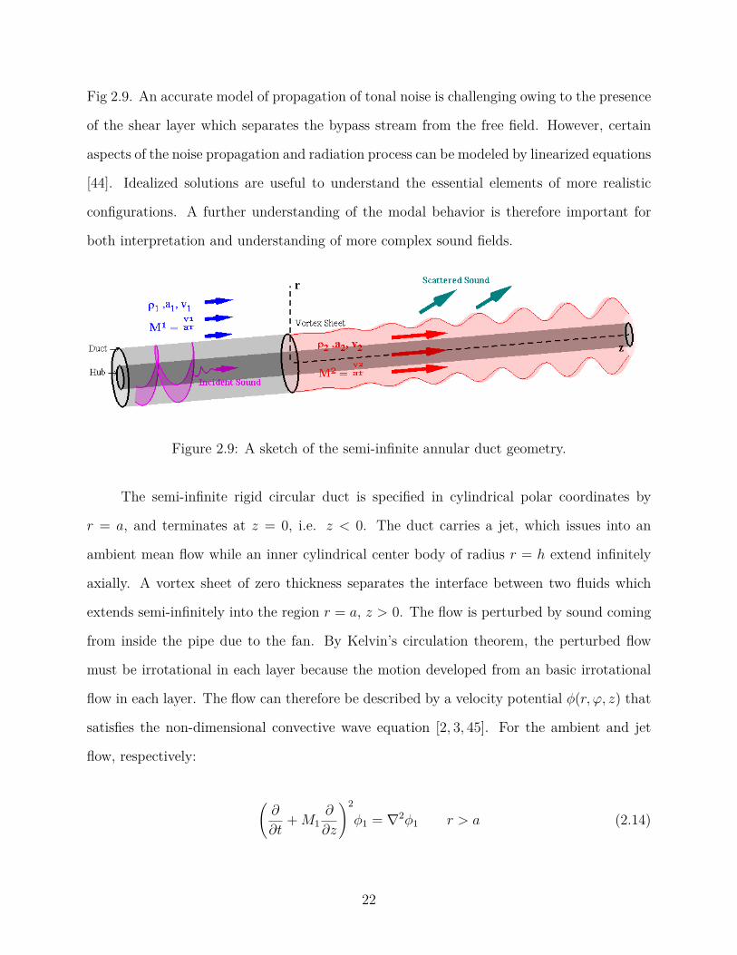
Fig 2.9. An accurate model of propagation of tonal noise is challenging owing to the presence
of the shear layer which separates the bypass stream from the free field. However, certain
aspects of the noise propagation and radiation process can be modeled by linearized equations
[44]. Idealized solutions are useful to understand the essential elements of more realistic
configurations. A further understanding of the modal behavior is therefore important for
both interpretation and understanding of more complex sound fields.
Figure 2.9: A sketch of the semi-infinite annular duct geometry.
The semi-infinite rigid circular duct is specified in cylindrical polar coordinates by
r = a, and terminates at z = 0, i.e. z < 0. The duct carries a jet, which issues into an
ambient mean flow while an inner cylindrical center body of radius r = h extend infinitely
axially. A vortex sheet of zero thickness separates the interface between two fluids which
extends semi-infinitely into the region r = a, z > 0. The flow is perturbed by sound coming
from inside the pipe due to the fan. By Kelvin’s circulation theorem, the perturbed flow
must be irrotational in each layer because the motion developed from an basic irrotational
flow in each layer. The flow can therefore be described by a velocity potential φ(r, ϕ, z) that
satisfies the non-dimensional convective wave equation [2, 3, 45]. For the ambient and jet
flow, respectively:
(∂
∂t+M1
∂
∂z
)2
φ1 = ∇2φ1 r > a (2.14)
22
C21
(∂
∂t+M2
∂
∂z
)2
φ2 = ∇2φ2 h < r < a (2.15)
Note that the non-dimensional quantities M1,M2 are the Mach number in terms of the
sound speed in the free stream, c1. That is, M2 is not the local Mach number. The ratio of
the speed of sound is denoted C1 = c1/c2. The hard wall, kinematic, dynamic, far field , and
Kutta boundary conditions are:
∂φ
∂r(a, ϕ, z) = 0, z ≤ 0 (2.16)
(∂
∂t+M1
∂
∂z
)η(z) =
(∂
∂t+M2
∂
∂z
)η(z) = ∂φ
∂r(a±, z) z ≥ 0 (2.17)
(∂
∂t+M1
∂
∂z
)φ1(a+, z) = D1
(∂
∂t+M2
∂
∂z
)φ2(a−, z) z ≥ 0 (2.18)
φ→ 0 as |z| → ∞ φ = O(|z| 32 ) as |z| → 0 (2.19)
where D1 = ρ2/ρ1 is the ratio of the jet and ambient densities and η(z) is the radial
displacement of the vortex sheet. We split the total acoustic field as the sum of the incident
wave φ and diffracted field ψ. The solution includes K, the Wiener-Hopf Kernel which
encapsulate the physical behavior of the scattered acoustic field [46].
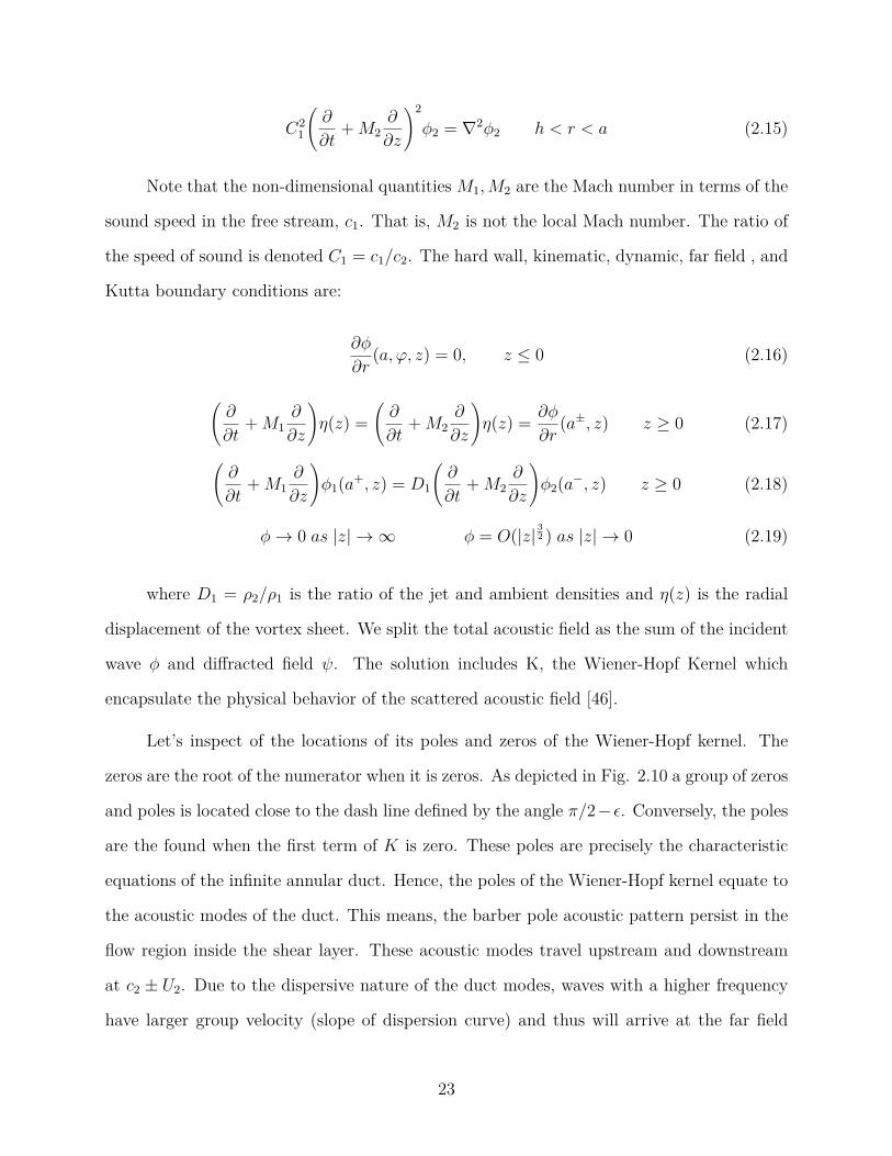
Let’s inspect of the locations of its poles and zeros of the Wiener-Hopf kernel. The
zeros are the root of the numerator when it is zeros. As depicted in Fig. 2.10 a group of zeros
and poles is located close to the dash line defined by the angle π/2− ε. Conversely, the poles
are the found when the first term of K is zero. These poles are precisely the characteristic
equations of the infinite annular duct. Hence, the poles of the Wiener-Hopf kernel equate to
the acoustic modes of the duct. This means, the barber pole acoustic pattern persist in the
flow region inside the shear layer. These acoustic modes travel upstream and downstream
at c2 ± U2. Due to the dispersive nature of the duct modes, waves with a higher frequency
have larger group velocity (slope of dispersion curve) and thus will arrive at the far field
23
Figure 2.10: Location of zeros (), and poles (•) of the Wiener-Hopf kernel for annular jetoperating with ω = 4, M2=5, M1 = 0.25, D1 = C1 =1, h=0 . Image from Rienstra [2].
.
sooner than waves with a lower frequency. Another set of zeros exist that are related to the
instability of the vortex sheet. In the case of a cold jet, the phase velocity according to high
frequency approximation is found as:
vp = M1 +M2
2 ± i
2
√1− (
√1 + (M2 −M1)2 − 2)2 (2.20)
Vortical modes convective velocities are similar to those predicted from Kelvin-Helmholtz
instability. When the jet is subsonic, i.e. M < 1 the second term is always imaginary and
represent the amplification of the instability which is driven by the difference of velocity
between the two streams. The real part correspond to waves moving at the average speed
of the two streams. This field is non-decaying in the downstream direction, and therefore
contributes to the far field. However, it is purely hydrodynamic (involves no pressure varia-
tions) and is only significant near the vortex sheet. Such growth cannot continue indefinitely
since at some stage the finite thickness of the shear layer will become important.
An interaction between acoustic and non acoustic modes takes place. Figure 2.11
24
↑ Mach lowers peak directivity toward exhaust
Figure 2.11: Pressure contours of semi-infinite duct (left), pressure directivity patterns inthe far field for various freestream velocities from Huang [3] (right).
displays the pressure contours and pressure directivity patterns with varying external flow
velocity while holding other parameters constant. The sound pressure perturbation contours
demonstrates the modal solution of the duct persist outside. As the sound reaches the
end, its radiates, convect, and refracts into the surrounding air. Furthermore, as the Mach
number of the ambient increases from 0 to 0.45, the peak directuvity pattern shift toward
the jet axis. A cone of cone of silence appears as the mean flow transport the acoustic
disturbances. Computational experiments using more realistic configurations show good
agreement with analytical results, and provides an understanding of the influence of the mean
flow convection/refraction effects. Fig. 2.12 displays instantaneous pressure field associated
for takeoff (left) and quiescent (right) conditions. Comparison of the images revels the
acoustic waves exiting the nozzle with a lower angle with respect to the exhaust [4]. This
deflection phenomenon confirms the interaction of the acoustic disturbance and shear flow.
2.4 Connecting Analytic Solutions to Noise Model
The development a model of radiating tonal noise from an exhaust requires an theoretical
understanding of characteristics of duct modes. Key findings are:
25
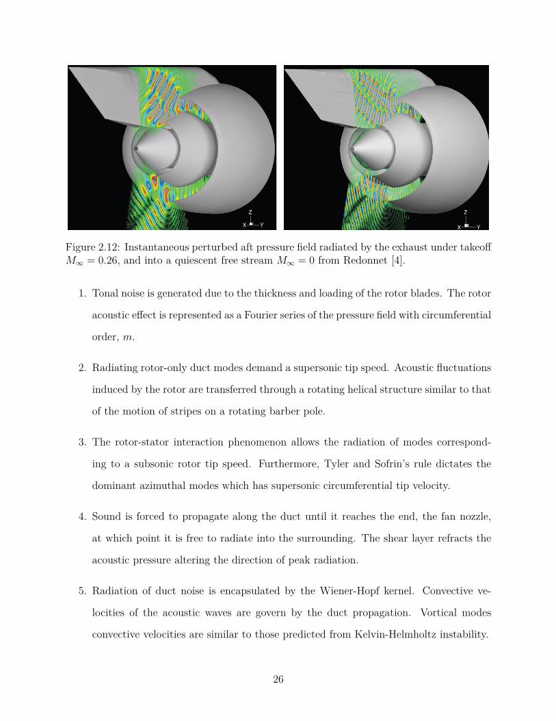
Figure 2.12: Instantaneous perturbed aft pressure field radiated by the exhaust under takeoffM∞ = 0.26, and into a quiescent free stream M∞ = 0 from Redonnet [4].
1. Tonal noise is generated due to the thickness and loading of the rotor blades. The rotor
acoustic effect is represented as a Fourier series of the pressure field with circumferential
order, m.
2. Radiating rotor-only duct modes demand a supersonic tip speed. Acoustic fluctuations
induced by the rotor are transferred through a rotating helical structure similar to that
of the motion of stripes on a rotating barber pole.
3. The rotor-stator interaction phenomenon allows the radiation of modes correspond-
ing to a subsonic rotor tip speed. Furthermore, Tyler and Sofrin’s rule dictates the
dominant azimuthal modes which has supersonic circumferential tip velocity.
4. Sound is forced to propagate along the duct until it reaches the end, the fan nozzle,
at which point it is free to radiate into the surrounding. The shear layer refracts the
acoustic pressure altering the direction of peak radiation.
5. Radiation of duct noise is encapsulated by the Wiener-Hopf kernel. Convective ve-
locities of the acoustic waves are govern by the duct propagation. Vortical modes
convective velocities are similar to those predicted from Kelvin-Helmholtz instability.
26
Kirchhoff or FWH surface
Figure 2.13: Pressure perturbation fields from Reboul [5].
Prediction of the acoustic far field is implemented by a cylindrical Kirchhoff surface
enclosing the exhaust of the turbofan. The surface is sufficiently close to the exhaust and
feels the footprint of the modal pressure disturbance generated by the rotor and rotor-stator
interaction as illustrated in Fig 2.13. The blade passage frequencies are known. Further-
more, numerous azimuthal microphone array surveys, have found the dominate radiating
(supersonic circumferential tip velocity) azimuthal modes as those predicted by Tyler and
Sorfin [47,48]. Thus, we assume that the azimuthal mode is determined by the Tyler-Sofrin
relation [19]
m = hB + kV (2.21)
where B is the number of blades on the fan and V is the number of stator vanes. On the
other hand, h and k is the harmonic, and a arbitrary integer, respectively. Observation of
spiral structure highlighted in finding 2, motivated prescribing the pressure perturbation on
the Kichhoff surface as helical traveling wave. Written mathematically,
pw ∝ ei(mϕ−ωt+kzz) (2.22)
27
wherem,ω, kz are the azimutal mode, angular frequency, and axial wavenumber, respectively.
Estimates of the wavenumber, kz (or more importantly the convective velocity) may be
obtained from the knowledge of the property of the Wiener-Hopf kernel. By assuming a
locally constant cross section the dispersion relation for azimuth mode m and h harmonic is
estimated by:
k±z,mn =−M2C
21 ±
√C2
1 − (1−M22C
21)(µmn
ω)2
1−M22C
21
(2.23)
where k0 is the acoustic frequency, M is the mean flow Mach number, kz,mn is the wave
number of the right (+) and left (−) traveling modes. Due to the dispersive nature of the
duct modes, waves with a higher frequency will propagate faster to the far field than longer
wavelength waves. µmn are the roots of the wall boundary condition.
d
dz[Ym(zh)]Jm(z)− d
dz[Jm(zh)]Ym(z) = 0 (2.24)
in which Jm(z) and Ym(z) are the Bessel function of the first and second kind of order
m, and h is the hub-to-tip ratio of the duct. Realistic wavenumber will deviate depending on
the area variation of the nozzle. Numerical optimization will provide the actual convective
velocity, but these analytical expressions provides an good start and sanity check of our
computational methods. Lastly, the amplification and decay of the acoustic waves due to
the duct geometry and shear layer influence are reproduced by an envelope function, po(z).
Combining these findings, the pressure prescribed on the surface is:
p(m, r0, z, ϕ, t) = p0(z)ei(mϕ−ωt) (2.25)
28
3
Cha
pter
Noise Source Modeling,
Parametrization, and Scattering
Prediction
So far, we discussed the principal sources of fan noise and their respective generating
mechanics. This chapter will propose a low-order, physics-based model of the aft fan
noise source. Here we start with a deterministic noise source model based on the wavepacket
ansatz. This model contain a finite set parameters that must be determined experimentally.
In the second half, we will discuss the reconstruction of the parameters of the wavepacket
model from measurements and computational scattering predictions.
3.1 Wavepacket Model Formulation
In a infinite annular duct with uniform flow, any acoustic field can be decomposed as a
sum of rotating mode patterns with circumferential and radial (order m and n) pressure
distributions. These are elementary solutions to the convective Helmholtz’s equation. The
sound is forced to propagate along the duct until it reaches the end, the fan nozzle, at
29
which point it is free to radiate into the surrounding. We aim to mimic on a cylindrical
surface the footprint of these modal structure generated by the fan. When viewed from the
outside the nacelle, the influence of these modal structure are approximated by a amplitude
modulated traveling wave on a control surface surrounding the exit of the nozzle. The
spatiotemporal amplification and decay behavior reflects the influence of the complex nozzle
geometry, rotor/stator interaction, and shear layer. For the sake of simplification, pylon/
bifurcation interaction, and non-symmertic effects are not considered. Low-order modeling
enables predictions of the radiated sound and its scattering around objects without inordinate
computational resources. This wavepacket model is based on the foundational work by Tam
and Burton [49], Cirghton and Huerre [50], Avital et al [51], and Papamoschou et al [16].
G
Figure 3.1: Fan noise source model with corresponding coordinate system, adapted fromSalvador Mayoral.
Consider a cylindrical surface Γ of radius ro that surrounds the fan whose axis is
aligned with the ducted fan center-line as sketch in Fig. 3.1. The fan exhaust is replaced by
a cylinder of radius r = r0 on which we prescribe the pressure pertubation [52]:
p(m, r0, z, ϕ, t) = p0(z)ei(mϕ−ωt) (3.1)
where r, ϕ, and z correspond to the cylindrical polar coordinates for radial position, az-
imuthal angle, and axial position, relative to the downstream axis, respectively. In addition,
30
m is the azimuthal mode, t represents time, and ω is the angular frequency. Lastly, p0(z)
describes the shape or modulation envelope of the wavepacket. This amplification-decay en-
velope represent the refraction phenomenon of the shear layer on the acoustic waveform, and
duct effects. A number of such partial field on the radiator surface is necessary to replicate
the characteristics of the pressure field at a given frequency. Specifically, the noise source
will be represented as an aggregation of deterministic partial fields that, overall, sum up
to capture the complex, extended and directional aft soundscape of the ducted fan. The
propagation of the pressure fluctuations away from the source is governed by the wave equa-
tion. In three-dimensional cylindrical polar coordinates the mathematical statement for a
stationary medium is:
1a2∞
∂2p
∂t2−[
1r
∂
∂r(r∂p∂r
) + 1r2∂2p
∂ϕ2 + ∂2p
∂z2
]= 0 (3.2)
To guarantee that the far field solution for p represents an outgoing wave (i.e. no reflections),
the Sommerfeld radiation condition at r →∞ is imposed
limr→∞
(∂p
∂r− ikp
)= 0 (3.3)
where k is the spatial frequency of a wave (acoustic wavenumber). The wave equation
(3.2) with the prescribed pressure boundary condition on the surface (3.1), along with the
Sommerfeld condition (3.3) may be solved using Fourier transform. Converting the acoustic
pressure from a time/space domain (ϕ, z, t) representation to the frequency/wave number
domain (m, kz, ω) can be accomplished using the multidimensional transform pair:
Pm(m, kz, ω) =∫ ∞−∞
∫ ∞−∞
∫ π
−πp(ϕ, z, t)e[i(ωt−kzz−mϕ)]dϕdtdz
p(ϕ, z, t) = 1(2π)3
∞∑m=−∞
∫ ∞−∞
∫ ∞−∞
Pm(m, kz, ω)e[−i(ωt−kzz−mϕ)]dωdkz (3.4)
where m, kz, ω are the azimuthal mode, axial wavenumber, and angular frequency. Summa-
31
tion over the azimuthal mode occurred since the wavenumber m is discrete. Transformation
of the wave equation to the frequency domain and simplification yield a second-order linear
differential equation with variable coefficient known as Bessel’s differential equation.
r2∂2Pm
∂r2 + r∂Pm
∂r+ (r2kr
2 −m2)Pm = 0 (3.5)
where kr is the radial wave number, kr =√k2 − k2
z . The general solution is given by:
Pm(r,m, kz, ω) = Cm1(k, ω)H(1)m (krr) + Cm2(k, ω)H(2)
m (krr) (3.6)
with Cm1, Cm2 as constants and P denotes the spatial Fourier transform of p(z). The
Hankel function of the first and second kind, H(1)m and H(2)
m are a linear combination of
Bessel functions of the first and second kind defined as
H(1)m (z) = Jm(z) + iYm(z) H(2)
m (z) = Jm(z)− iYm(z) (3.7)
010
2030
4050
-1
0
1
2
-2
-1.5
-1
-0.5
0
0.5
1
z
Hankel Function of First Kind
Real
Imaginary
H0(1) (z)
H1(1) (z)
H2(1) (z)
010
2030
4050
-1
0
1
2
-2
-1.5
-1
-0.5
0
0.5
1
1.5
2
z
Hankel Function of Second Kind
Real
Imaginary
H0(2) (z)
H1(2) (z)
H2(2) (z)
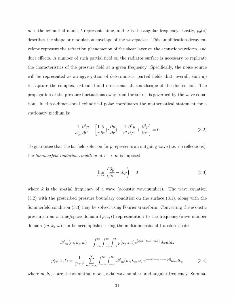
Figure 3.2: Graph of the Hankel function of the first and second kind in the complex plane.
Fig 3.2 plots the general behavior of the complex value function. The Hankel functions
form spirals, spinning around in the complex plane. Spirals can be either left-handed or
32
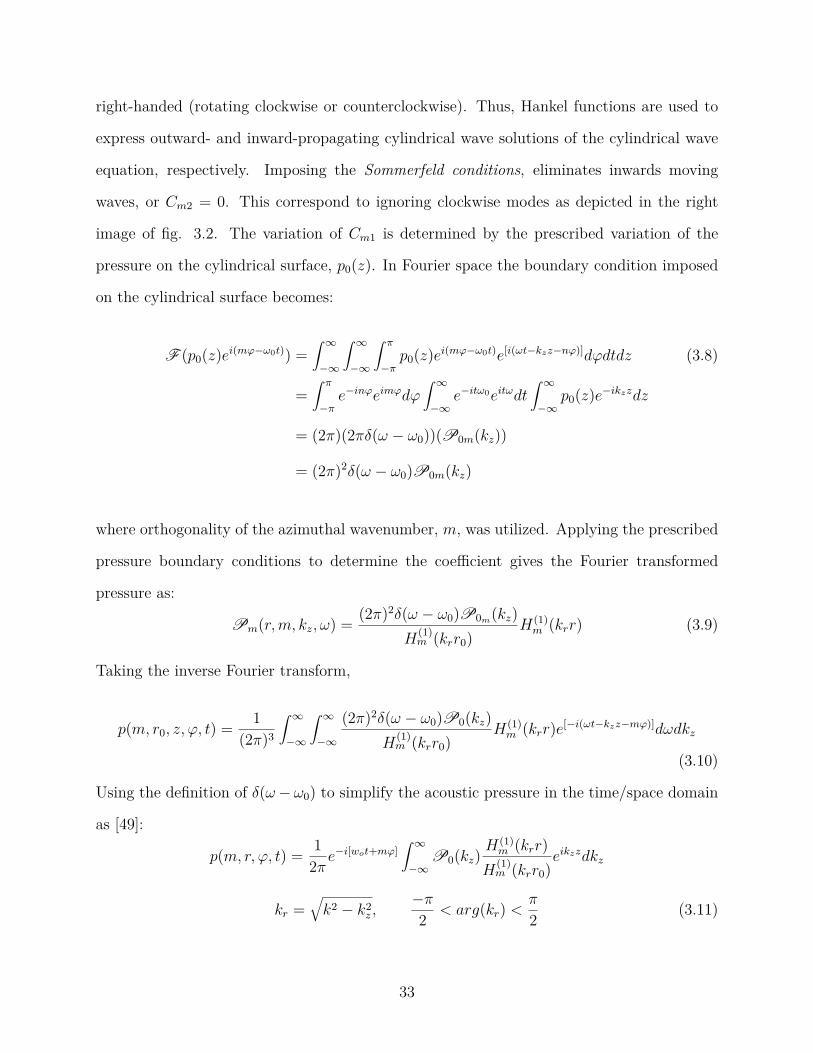
right-handed (rotating clockwise or counterclockwise). Thus, Hankel functions are used to
express outward- and inward-propagating cylindrical wave solutions of the cylindrical wave
equation, respectively. Imposing the Sommerfeld conditions, eliminates inwards moving
waves, or Cm2 = 0. This correspond to ignoring clockwise modes as depicted in the right
image of fig. 3.2. The variation of Cm1 is determined by the prescribed variation of the
pressure on the cylindrical surface, p0(z). In Fourier space the boundary condition imposed
on the cylindrical surface becomes:
F (p0(z)ei(mϕ−ω0t)) =∫ ∞−∞
∫ ∞−∞
∫ π
−πp0(z)ei(mϕ−ω0t)e[i(ωt−kzz−nϕ)]dϕdtdz (3.8)
=∫ π
−πe−inϕeimϕdϕ
∫ ∞−∞
e−itω0eitωdt∫ ∞−∞
p0(z)e−ikzzdz
= (2π)(2πδ(ω − ω0))(P0m(kz))
= (2π)2δ(ω − ω0)P0m(kz)
where orthogonality of the azimuthal wavenumber, m, was utilized. Applying the prescribed
pressure boundary conditions to determine the coefficient gives the Fourier transformed
pressure as:
Pm(r,m, kz, ω) = (2π)2δ(ω − ω0)P0m(kz)H
(1)m (krr0)
H(1)m (krr) (3.9)
Taking the inverse Fourier transform,
p(m, r0, z, ϕ, t) = 1(2π)3
∫ ∞−∞
∫ ∞−∞
(2π)2δ(ω − ω0)P0(kz)H
(1)m (krr0)
H(1)m (krr)e[−i(ωt−kzz−mϕ)]dωdkz
(3.10)
Using the definition of δ(ω−ω0) to simplify the acoustic pressure in the time/space domain
as [49]:
p(m, r, ϕ, t) = 12πe
−i[wot+mϕ]∫ ∞−∞
P0(kz)H(1)m (krr)
H(1)m (krr0)
eikzzdkz
kr =√k2 − k2
z ,−π2 < arg(kr) <
π
2 (3.11)
33
where the argument (or phase) of the radial eigenvalue kr is bounded to ensure the behavior of
H(1)m (krr) forms a radially outward spiral in the far field- i.e. satisfies Sommerfeld condition.
The formulation recreates the radiative and nonradiative behavior typical of helical waves.
A wavepacket moving with a phase speed that is subsonic generates an evanescent acoustic
field. Conversely, a wave moving with a supersonic phase speed radiates. Equation 3.11 is
the exact solution to the linearized acoustic problem, valid everywhere for r ≥ r0. Once the
wavepacket shape p0(z) is determined, Eq. 3.11 yields the incident field pi on the object
surface and at the field points.
𝑝0(𝑧) න−∞
∞
𝑒𝑖𝑘𝑧𝑧𝑑𝑘𝑧𝒫0(𝑘𝑧)
Fourier Trans.
𝑝𝑒𝑥𝑎𝑐𝑡(𝑧, 𝑟)
Mic r position
𝐻𝑚1
𝑧 = 𝐽𝑚 𝑧 + 𝑖𝑌𝑚(𝑧)
Mic z positionMic position
envelope shape
×𝐻𝑚(1)
𝑘𝑟𝑟
𝐻𝑚1(𝑘𝑟𝑟0)
Kernel
Inverse Fourier Transform
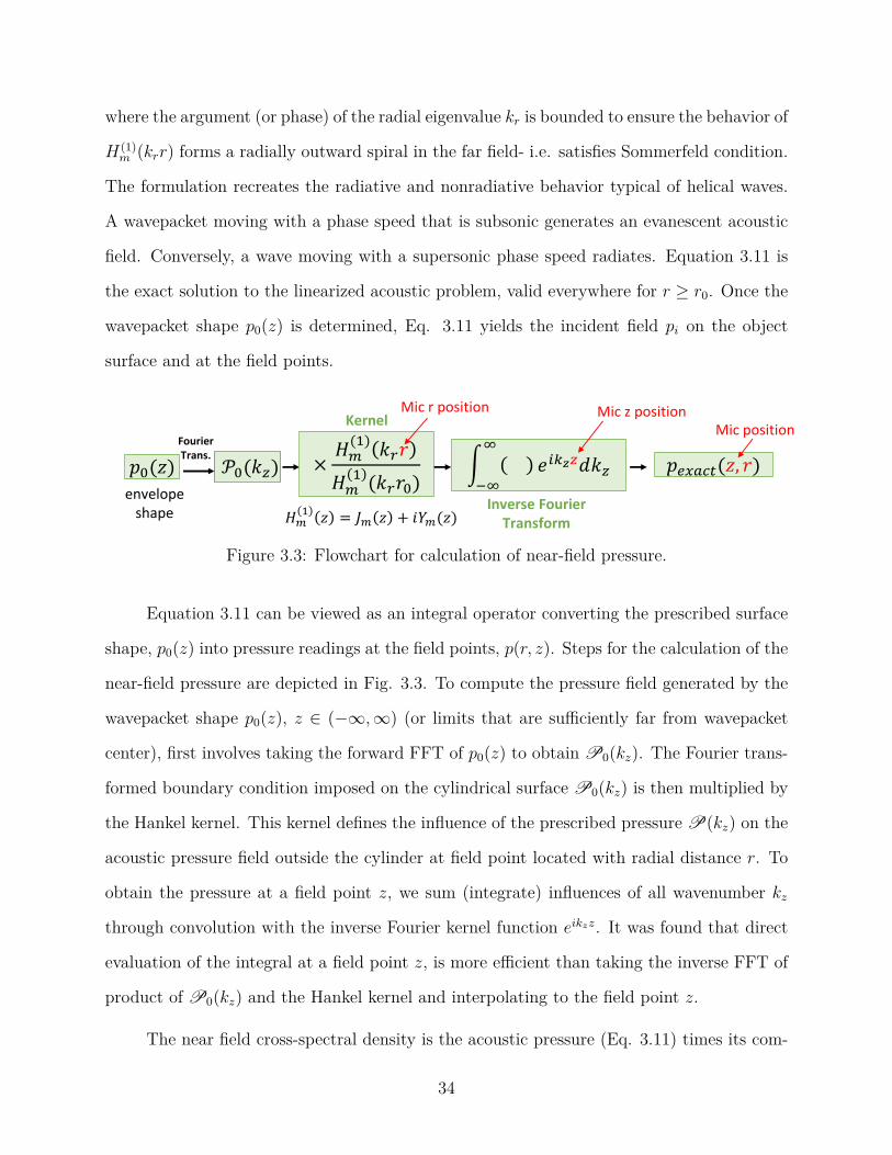
Figure 3.3: Flowchart for calculation of near-field pressure.
Equation 3.11 can be viewed as an integral operator converting the prescribed surface
shape, p0(z) into pressure readings at the field points, p(r, z). Steps for the calculation of the
near-field pressure are depicted in Fig. 3.3. To compute the pressure field generated by the
wavepacket shape p0(z), z ∈ (−∞,∞) (or limits that are sufficiently far from wavepacket
center), first involves taking the forward FFT of p0(z) to obtain P0(kz). The Fourier trans-
formed boundary condition imposed on the cylindrical surface P0(kz) is then multiplied by
the Hankel kernel. This kernel defines the influence of the prescribed pressure P(kz) on the
acoustic pressure field outside the cylinder at field point located with radial distance r. To
obtain the pressure at a field point z, we sum (integrate) influences of all wavenumber kz
through convolution with the inverse Fourier kernel function eikzz. It was found that direct
evaluation of the integral at a field point z, is more efficient than taking the inverse FFT of
product of P0(kz) and the Hankel kernel and interpolating to the field point z.
The near field cross-spectral density is the acoustic pressure (Eq. 3.11) times its com-
34
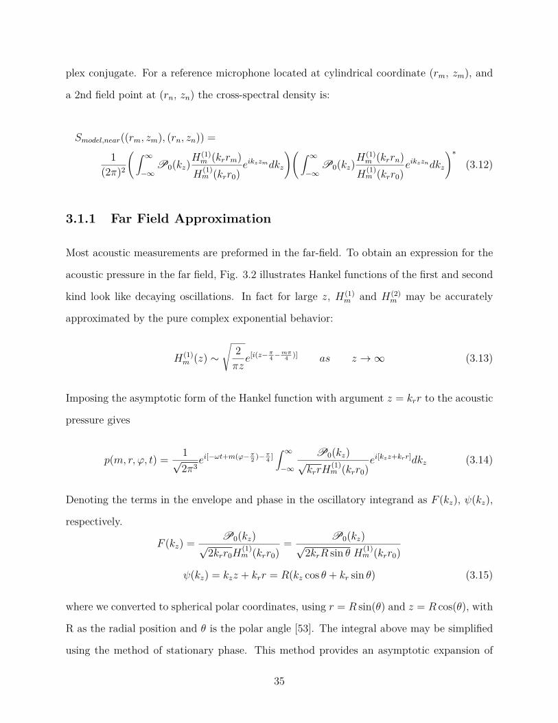
plex conjugate. For a reference microphone located at cylindrical coordinate (rm, zm), and
a 2nd field point at (rn, zn) the cross-spectral density is:
Smodel,near((rm, zm), (rn, zn)) =
1(2π)2
(∫ ∞−∞
P0(kz)H(1)m (krrm)
H(1)m (krr0)
eikzzmdkz
)(∫ ∞−∞
P0(kz)H(1)m (krrn)
H(1)m (krr0)
eikzzndkz
)∗(3.12)
3.1.1 Far Field Approximation
Most acoustic measurements are preformed in the far-field. To obtain an expression for the
acoustic pressure in the far field, Fig. 3.2 illustrates Hankel functions of the first and second
kind look like decaying oscillations. In fact for large z, H(1)m and H(2)
m may be accurately
approximated by the pure complex exponential behavior:
H(1)m (z) ∼
√2πze[i(z−π4−
mπ4 )] as z →∞ (3.13)
Imposing the asymptotic form of the Hankel function with argument z = krr to the acoustic
pressure gives
p(m, r, ϕ, t) = 1√2π3
ei[−ωt+m(ϕ−π2 )−π4 ]∫ ∞−∞
P0(kz)√krrH
(1)m (krr0)
ei[kzz+krr]dkz (3.14)
Denoting the terms in the envelope and phase in the oscillatory integrand as F (kz), ψ(kz),
respectively.
F (kz) = P0(kz)√2krr0H
(1)m (krr0)
= P0(kz)√2krR sin θ H(1)
m (krr0)
ψ(kz) = kzz + krr = R(kz cos θ + kr sin θ) (3.15)
where we converted to spherical polar coordinates, using r = R sin(θ) and z = R cos(θ), with
R as the radial position and θ is the polar angle [53]. The integral above may be simplified
using the method of stationary phase. This method provides an asymptotic expansion of
35
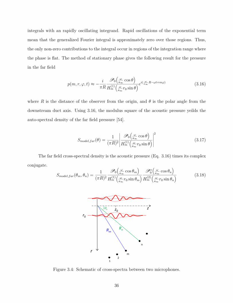
integrals with an rapidly oscillating integrand. Rapid oscillations of the exponential term
mean that the generalized Fourier integral is approximately zero over those regions. Thus,
the only non-zero contributions to the integral occur in regions of the integration range where
the phase is flat. The method of stationary phase gives the following result for the pressure
in the far field
p(m, r, ϕ, t) ≈ − i
πR
P0(ωa∞
cos θ)
H(1)m
(ωa∞r0 sin θ
)ei( ωa∞
R−ωt+mϕ) (3.16)
where R is the distance of the observer from the origin, and θ is the polar angle from the
downstream duct axis. Using 3.16, the modulus square of the acoustic pressure yeilds the
auto-spectral density of the far field pressure [54].
Smodel,far(θ) = 1(πR)2
∣∣∣∣∣∣P0
(ωa∞
cos θ)
H(1)m
(ωa∞r0 sin θ
)∣∣∣∣∣∣2
(3.17)
The far field cross-spectral density is the acoustic pressure (Eq. 3.16) times its complex
conjugate.
Smodel,far(θm, θn) = 1(πR)2
P0(ωa∞
cos θm)
H(1)m
(ωa∞r0 sin θm
) P∗0
(ωa∞
cos θn)
H(2)m
(ωa∞r0 sin θn
) (3.18)
z
r
Rm
qn z0r0
12
m
n
Rn
Figure 3.4: Schematic of cross-spectra between two microphones.
36
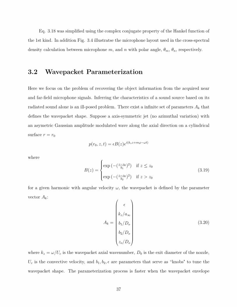
Eq. 3.18 was simplified using the complex conjugate property of the Hankel function of
the 1st kind. In addition Fig. 3.4 illustratse the microphone layout used in the cross-spectral
density calculation between microphone m, and n with polar angle, θm, θn, respectively.
3.2 Wavepacket Parameterization
Here we focus on the problem of recovering the object information from the acquired near
and far-field microphone signals. Inferring the characteristics of a sound source based on its
radiated sound alone is an ill-posed problem. There exist a infinite set of parameters Ak that
defines the wavepacket shape. Suppose a axis-symmetric jet (no azimuthal variation) with
an asymetric Gaussian amplitude modulated wave along the axial direction on a cylindrical
surface r = r0
p(r0, z, t) = εB(z)ei(kzz+mϕ−ωt)
where
B(z) =
exp (−( z−z0
b1)2) if z ≤ z0
exp (−( z−z0b2
)2) if z > z0
(3.19)
for a given harmonic with angular velocity ω, the wavepacket is defined by the parameter
vector Ak:
Ak =
ε
kz/a∞
b1/Do
b2/Do
zo/Do
(3.20)
where kz = ω/Uc is the wavepacket axial wavenumber, D0 is the exit diameter of the nozzle,
Uc is the convective velocity, and b1, b2, ε are parameters that serve as “knobs" to tune the
wavepacket shape. The parameterization process is faster when the wavepacket envelope
37
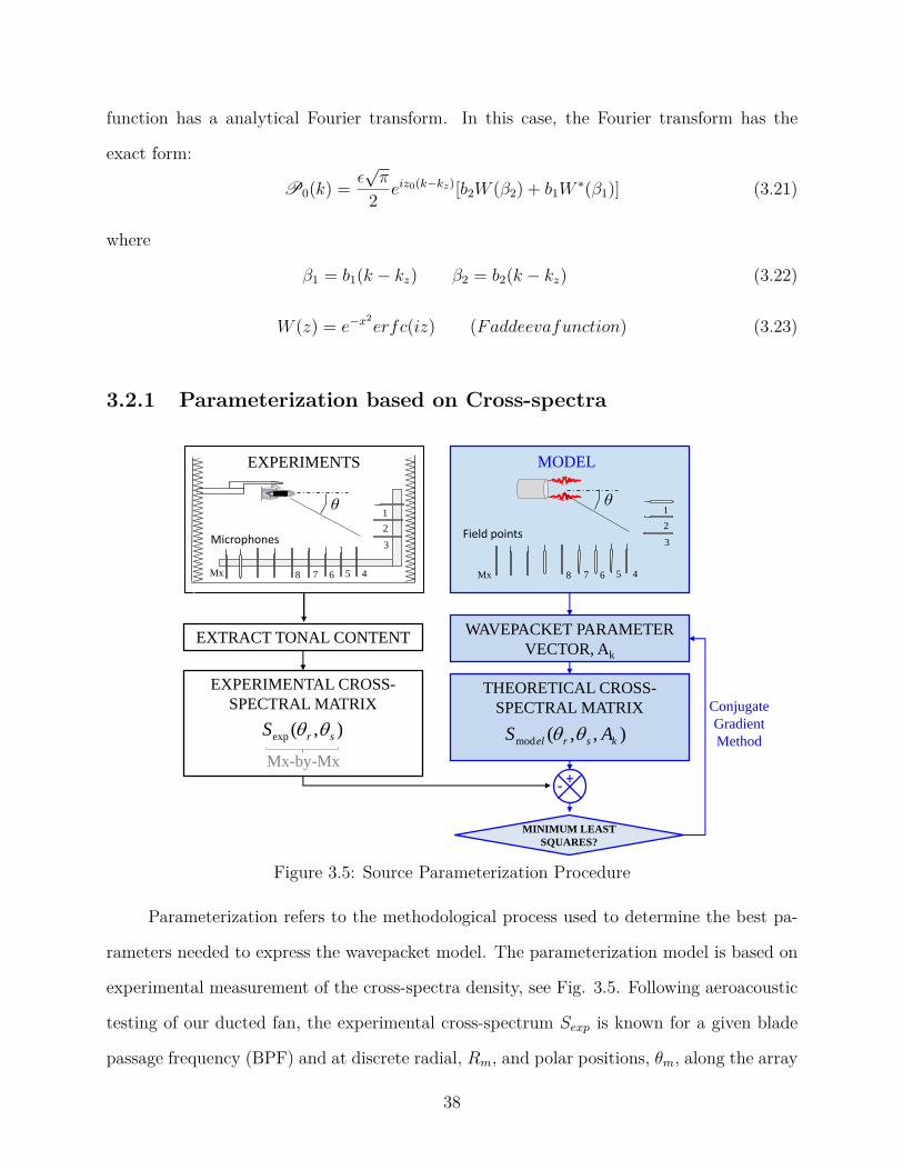
function has a analytical Fourier transform. In this case, the Fourier transform has the
exact form:
P0(k) = ε√π
2 eiz0(k−kz)[b2W (β2) + b1W∗(β1)] (3.21)
where
β1 = b1(k − kz) β2 = b2(k − kz) (3.22)
W (z) = e−x2erfc(iz) (Faddeevafunction) (3.23)
3.2.1 Parameterization based on Cross-spectra
WAVEPACKET PARAMETER
VECTOR, Ak
EXTRACT TONAL CONTENT
EXPERIMENTAL CROSS-
SPECTRAL MATRIXTHEORETICAL CROSS-
SPECTRAL MATRIX
),,(mod ksrel AS ),(exp srS
MINIMUM LEAST
SQUARES?
Conjugate
Gradient
Method
Field points
MODEL
θ
Microphones
EXPERIMENTS
θ1
2
3
Mx 45678
Mx-by-Mx
1
2
3
Mx 45678
+-
Figure 3.5: Source Parameterization Procedure
Parameterization refers to the methodological process used to determine the best pa-
rameters needed to express the wavepacket model. The parameterization model is based on
experimental measurement of the cross-spectra density, see Fig. 3.5. Following aeroacoustic
testing of our ducted fan, the experimental cross-spectrum Sexp is known for a given blade
passage frequency (BPF) and at discrete radial, Rm, and polar positions, θm, along the array
38
consisting of Mx microphones (m = 1, . . . ,Mx). For a given BPF, the azimutal mode m
is given by Tyler and Sofrin’s rule. A starting value of the wavenumber kz is estimated
from the analytical dispersion relation. The minimization process aims to select the optimal
parameter vector Ak in a way that minimizes the difference between the modeled Smodel(f)
and the experimental cross-spectral density Sexp(f) at all the measurement polar angles.
The parameter vector Ak is obtained through the least-square minimization of:
F (Ak) = 1M
M∑m,n=1
∣∣∣∣∣S∗exp(θm, θn)− S∗model(θm, θn, Ak)
S∗exp(θm, θn)
∣∣∣∣∣2
(3.24)
where the function sums over the unique values of the cross-spectra matrix consisting of
entries on and above the main diagonal. For a experiment with Mx microphones, the upper
limit isM = Mx (Mx+1)/2. The superscript, ∗ represent the normalized distribution. This
minimization scheme aims to match the normalized modeled intensity distribution S∗model to
the experimental intensity distribution S∗exp. We are only interested in matching the shape
(directivity) of the polar intensity distribution, and not so much its absolute value. Thus,
the modeled and experimental intensities are normalized by their corresponding maximum
value
S∗model(θm, θn, Ak) = Smodel(θm, θn, Ak)Smodel,max
S∗exp = Sexp(θm, θn)Sexp,max
(3.25)
where Sexp,max and Smodel, max denotes the maximum real-part of the cross spectra matrix for
the experimental and model, respectively. A FORTRAN code was developed to postprocess
the Vold-Kalman filtered tonal noise data. A schematic of the code is shown in Fig. 3.7. The
minimization process of the above equation uses the Restarted Conjugate Gradient method
of Shanno and Phua [55]. The Hankel Functions were determined from TOM algorithm
644 [56]. Once the wavepacket shaped is matched, the absolute levels are scaled to the
appropriate amplitude.
39
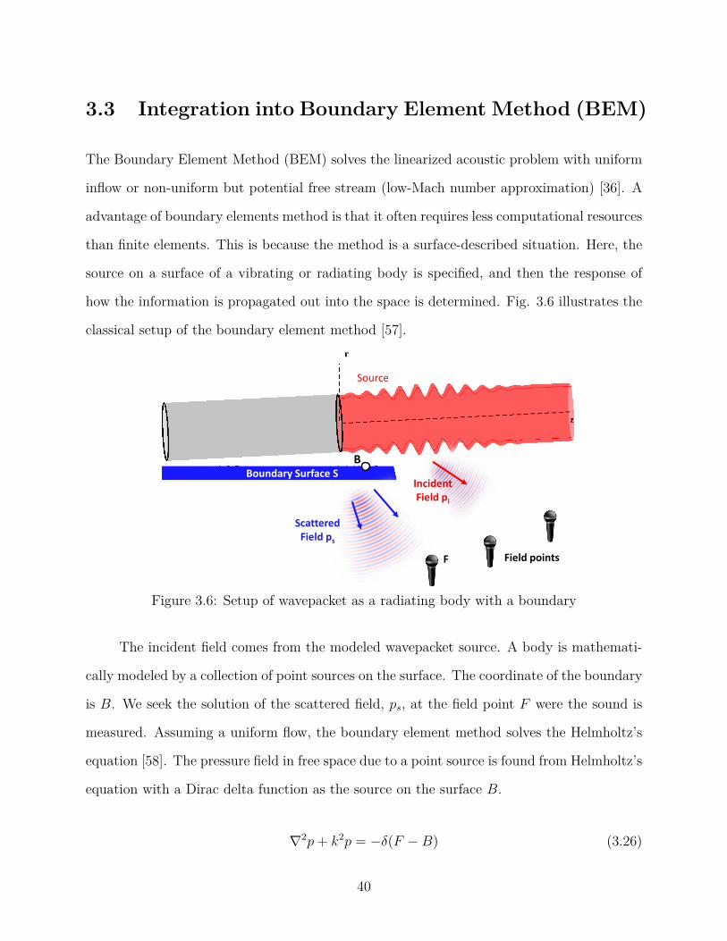
3.3 Integration into Boundary Element Method (BEM)
The Boundary Element Method (BEM) solves the linearized acoustic problem with uniform
inflow or non-uniform but potential free stream (low-Mach number approximation) [36]. A
advantage of boundary elements method is that it often requires less computational resources
than finite elements. This is because the method is a surface-described situation. Here, the
source on a surface of a vibrating or radiating body is specified, and then the response of
how the information is propagated out into the space is determined. Fig. 3.6 illustrates the
classical setup of the boundary element method [57].
Source
Boundary Surface SIncident Field pi
Scattered Field ps
Field pointsF
B
Figure 3.6: Setup of wavepacket as a radiating body with a boundary
The incident field comes from the modeled wavepacket source. A body is mathemati-
cally modeled by a collection of point sources on the surface. The coordinate of the boundary
is B. We seek the solution of the scattered field, ps, at the field point F were the sound is
measured. Assuming a uniform flow, the boundary element method solves the Helmholtz’s
equation [58]. The pressure field in free space due to a point source is found from Helmholtz’s
equation with a Dirac delta function as the source on the surface B.
∇2p+ k2p = −δ(F −B) (3.26)
40
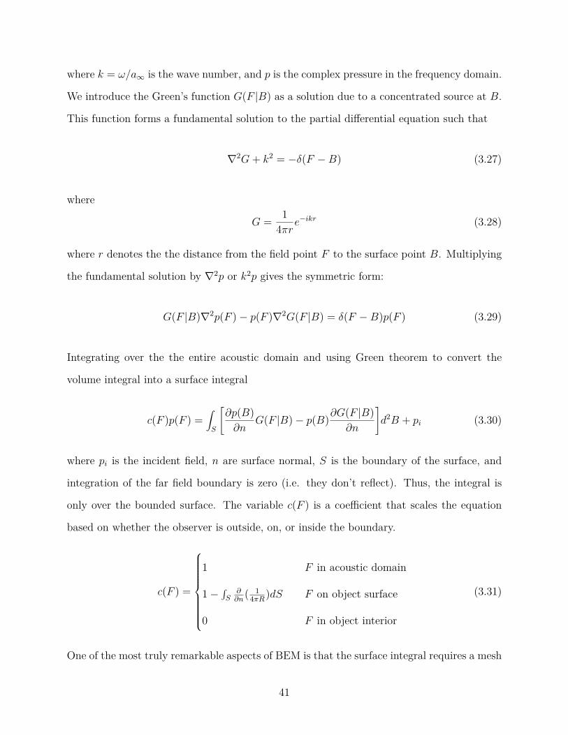
where k = ω/a∞ is the wave number, and p is the complex pressure in the frequency domain.
We introduce the Green’s function G(F |B) as a solution due to a concentrated source at B.
This function forms a fundamental solution to the partial differential equation such that
∇2G+ k2 = −δ(F −B) (3.27)
where
G = 14πre
−ikr (3.28)
where r denotes the the distance from the field point F to the surface point B. Multiplying
the fundamental solution by ∇2p or k2p gives the symmetric form:
G(F |B)∇2p(F )− p(F )∇2G(F |B) = δ(F −B)p(F ) (3.29)
Integrating over the the entire acoustic domain and using Green theorem to convert the
volume integral into a surface integral
c(F )p(F ) =∫S
[∂p(B)∂n
G(F |B)− p(B)∂G(F |B)∂n
]d2B + pi (3.30)
where pi is the incident field, n are surface normal, S is the boundary of the surface, and
integration of the far field boundary is zero (i.e. they don’t reflect). Thus, the integral is
only over the bounded surface. The variable c(F ) is a coefficient that scales the equation
based on whether the observer is outside, on, or inside the boundary.
c(F ) =
1 F in acoustic domain
1−∫S
∂∂n
( 14πR)dS F on object surface
0 F in object interior
(3.31)
One of the most truly remarkable aspects of BEM is that the surface integral requires a mesh
41
of a surface rather than a solid volume. Thus, this formulation simplifies the labor required
to mesh complex geometries. Typically, the boundary surface is discretize using triangular
meshes with a resolution of 8 nodes per wavelength. Boundary element formulation give
rise to dense matrices. This means that the storage requirements grows according to O(N2)
for a system of N nodes. The BEM code developed by T.W. Wu was used for scattering
predictions [59].
42
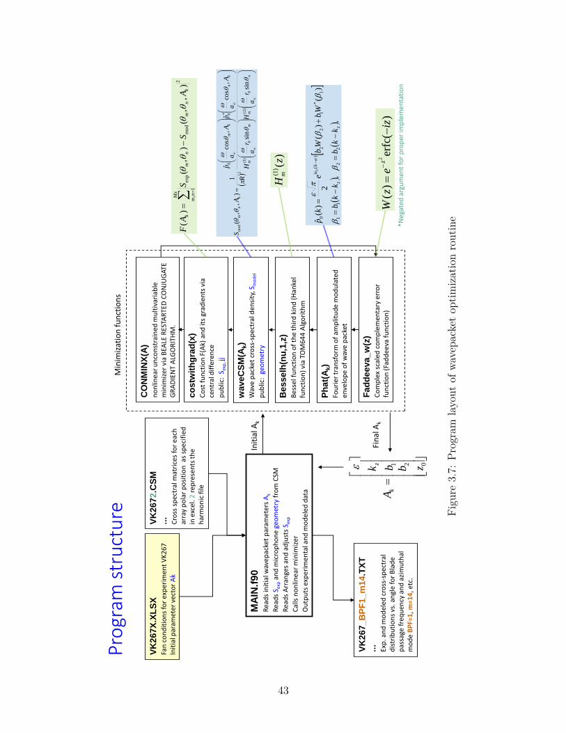
Pro
gram
str
uct
ure
MA
IN.f
90
Rea
ds
init
ial w
avep
acke
tp
aram
eter
s A
k
Rea
ds
S exp
and
mic
rop
ho
ne
geo
met
ry f
rom
CSM
Rea
ds
Arr
ange
s an
d a
dju
sts
S exp
Cal
ls n
on
linea
r m
inim
izer
Ou
tpu
ts e
xper
imen
tal a
nd
mo
del
ed
dat
a
CO
NM
INX
(A)
no
nlin
ear
un
con
stra
ined
mu
ltiv
aria
ble
m
inim
izer
via
BEA
LE R
ESTA
RTE
D C
ON
JUG
ATE
GR
AD
IEN
T A
LGO
RIT
HM
.
co
stw
ith
gra
d(x
)C
ost
fu
nct
ion
F(A
k) a
nd
its
grad
ien
ts v
ia
cen
tral
dif
fere
nce
pu
blic
: S e
xp, j
j
wave
CS
M(A
k)
Wav
e p
acke
t cr
oss
-sp
ectr
al d
ensi
ty, S
mo
del
pu
blic
: ge
om
etry
Init
ial A
k
Fin
al A
k
Min
imiz
atio
n f
un
ctio
ns
VK
26
7X
.XL
SX
Fan
co
nd
itio
ns
for
exp
erim
ent
VK
26
7
Init
ial p
aram
eter
vec
tor
Ak
VK
26
72.C
SM
...
Cro
ss s
pec
tral
mat
rice
s fo
r ea
ch
arra
y p
ola
r p
osi
tio
n a
s sp
ecif
ied
in
exc
el. 2
rep
rese
nts
th
e h
arm
on
ic f
ile
VK
26
7_
BP
F1
_m
14.T
XT
...
Exp
. an
d m
od
ele
d c
ross
-sp
ectr
al
dis
trib
uti
on
s vs
. an
gle
for
Bla
de
pas
sage
fre
qu
ency
an
d a
zim
uth
al
mo
de BPF=1
, m=14
, etc
.
Be
sse
lh(n
u,1
,z)
Bes
sel f
un
ctio
n o
f th
e th
ird
kin
d (
Han
kel
fun
ctio
n) v
ia T
OM
64
4 A
lgo
rith
m
Ph
at(
Ak)
Fou
rier
tra
nsf
orm
of
amp
litu
de
mo
du
late
d
enve
lop
e o
f w
ave
pac
ket
Fa
dd
ee
va
_w
(z)
Co
mp
lex
scal
ed c
om
ple
men
tary
err
or
fun
ctio
n (F
add
eeva
fun
ctio
n)
Mx n
m
kn
mn
mk
AS
SA
F1
,
2
mo
dex
p)
,,
()
,(
)(
nm
mm
kn
km
kn
m
ra
Hr
aH
Aa
pA
ap
RA
S
sin
sin
,co
sˆ
,co
sˆ
1)
,,
(
0
)2(
0
)1(
* 00
2m
od
)(
)1(
zH
m
,
,
)(
)(
2)
(ˆ
22
11
1
*
12
2
)(
00
zz
kiz
kk
bk
kb
Wb
Wb
ek
p
)(
erfc
)(
2
ize
zW
z
*Neg
ated
arg
um
ent
for
pro
per
imp
lem
enta
tio
n
021 zbbk
Az
k
Figu
re3.7:
Program
layout
ofwa
vepa
cket
optim
izationroutine
43
4
Cha
pter
Experimental Details
4.1 Ducted Fan Rig
The experimental effort entailed the design and construction of a small-scaled ducted fan
rig that includes all the relevant components of the turbofan engine and simulates accu-
rately the sound emission by the fan of such engines. The scale of the fan is approximately
1:38, based on a full-scale inlet diameter of 2.67 m (105 in.) [29]. The fan was designed
to simulate the low fan pressure ratio (high bypass ratio) operation of a geared turbofan
engine. Various design elements of the rotor and stators were extracted from published re-
ports based on NASA/GE Source Diagnostic Test (SDT), particularly Refs. [22,24,25]. The
rotor and stator counts were 14 and 24, respectively, giving a rotor-stator ratio of 0.58. The
relatively low counts was selected for manufacturing considerations; however, having gained
experience with the manufacturing process, higher counts will be possible in the future. The
aerodynamic design process begins with non-negotiable characteristics that the compressor
must meet as documented in Table 4.1. These specifications are constrained by the power
capacity of the brushless motors.
Preliminary design and layout of the engine involves working first with simple one-
dimensional mean-line analysis. A schematic for the mean line (one-dimensional) calculation
stations is illustrated in Fig 4.1. Corresponding velocity triangles are drawn in the lower
44
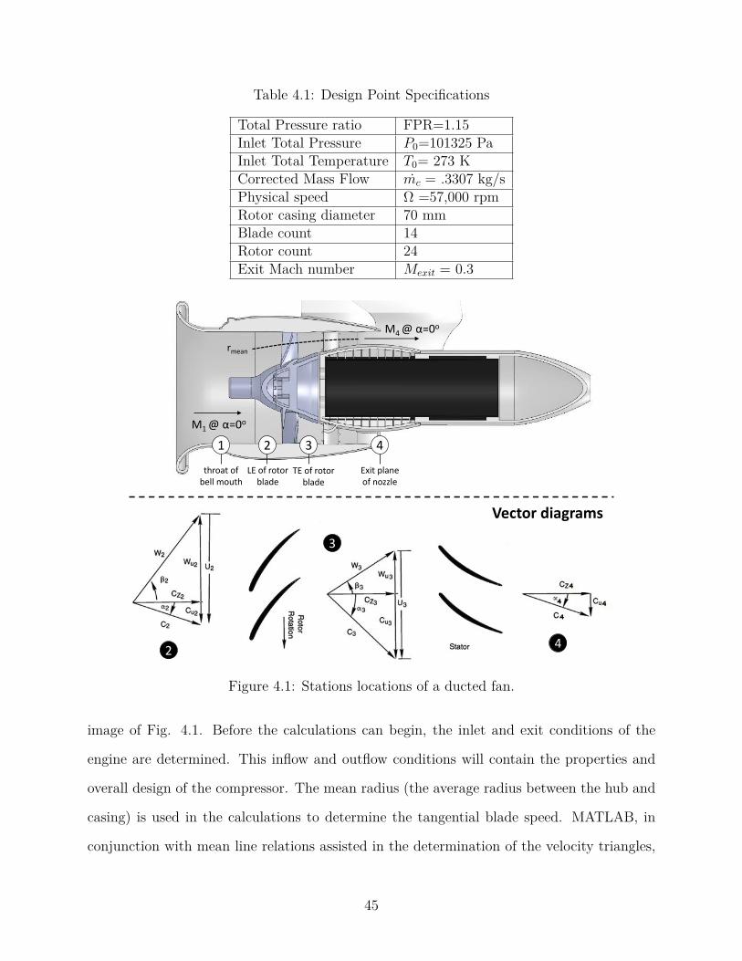
Table 4.1: Design Point Specifications
Total Pressure ratio FPR=1.15Inlet Total Pressure P0=101325 PaInlet Total Temperature T0= 273 KCorrected Mass Flow mc = .3307 kg/sPhysical speed Ω =57,000 rpmRotor casing diameter 70 mmBlade count 14Rotor count 24Exit Mach number Mexit = 0.3
1 2 3 4
throat of bell mouth
LE of rotor blade
TE of rotor blade
Exit plane of nozzle
M1 @ α=0o
M4 @ α=0o
rmean
2
3
4
Vector diagrams
Figure 4.1: Stations locations of a ducted fan.
image of Fig. 4.1. Before the calculations can begin, the inlet and exit conditions of the
engine are determined. This inflow and outflow conditions will contain the properties and
overall design of the compressor. The mean radius (the average radius between the hub and
casing) is used in the calculations to determine the tangential blade speed. MATLAB, in
conjunction with mean line relations assisted in the determination of the velocity triangles,
45
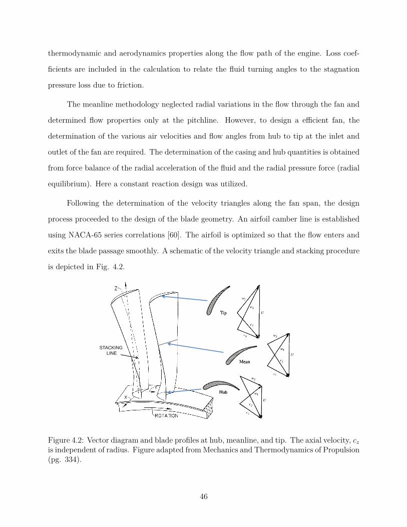
thermodynamic and aerodynamics properties along the flow path of the engine. Loss coef-
ficients are included in the calculation to relate the fluid turning angles to the stagnation
pressure loss due to friction.
The meanline methodology neglected radial variations in the flow through the fan and
determined flow properties only at the pitchline. However, to design a efficient fan, the
determination of the various air velocities and flow angles from hub to tip at the inlet and
outlet of the fan are required. The determination of the casing and hub quantities is obtained
from force balance of the radial acceleration of the fluid and the radial pressure force (radial
equilibrium). Here a constant reaction design was utilized.
Following the determination of the velocity triangles along the fan span, the design
process proceeded to the design of the blade geometry. An airfoil camber line is established
using NACA-65 series correlations [60]. The airfoil is optimized so that the flow enters and
exits the blade passage smoothly. A schematic of the velocity triangle and stacking procedure
is depicted in Fig. 4.2.
STACKING
LINE
Figure 4.2: Vector diagram and blade profiles at hub, meanline, and tip. The axial velocity, czis independent of radius. Figure adapted fromMechanics and Thermodynamics of Propulsion(pg. 334).
46
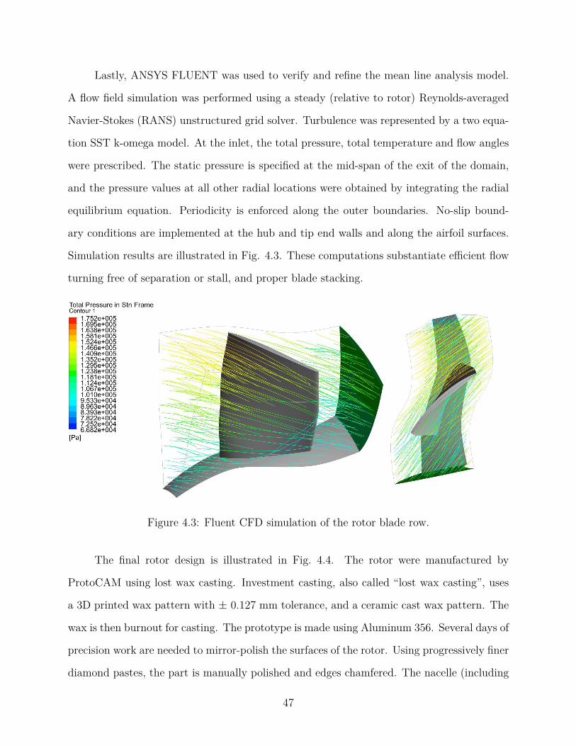
Lastly, ANSYS FLUENT was used to verify and refine the mean line analysis model.
A flow field simulation was performed using a steady (relative to rotor) Reynolds-averaged
Navier-Stokes (RANS) unstructured grid solver. Turbulence was represented by a two equa-
tion SST k-omega model. At the inlet, the total pressure, total temperature and flow angles
were prescribed. The static pressure is specified at the mid-span of the exit of the domain,
and the pressure values at all other radial locations were obtained by integrating the radial
equilibrium equation. Periodicity is enforced along the outer boundaries. No-slip bound-
ary conditions are implemented at the hub and tip end walls and along the airfoil surfaces.
Simulation results are illustrated in Fig. 4.3. These computations substantiate efficient flow
turning free of separation or stall, and proper blade stacking.
Figure 4.3: Fluent CFD simulation of the rotor blade row.
The final rotor design is illustrated in Fig. 4.4. The rotor were manufactured by
ProtoCAM using lost wax casting. Investment casting, also called “lost wax casting”, uses
a 3D printed wax pattern with ± 0.127 mm tolerance, and a ceramic cast wax pattern. The
wax is then burnout for casting. The prototype is made using Aluminum 356. Several days of
precision work are needed to mirror-polish the surfaces of the rotor. Using progressively finer
diamond pastes, the part is manually polished and edges chamfered. The nacelle (including
47
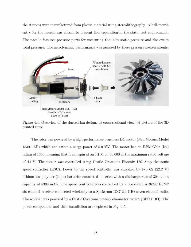
the stators) were manufactured from plastic material using stereolithography. A bell-mouth
entry for the nacelle was chosen to prevent flow separation in the static test environment.
The nacelle features pressure ports for measuring the inlet static pressure and the outlet
total pressure. The aerodynamic performance was assessed by these pressure measurements.
70-mm diameter
nacelle with bell
mouth inlet
14-blade
rotor24 stators
Neu Motors Model 1530-1.5D
brushless DC motor
5000 W (6 hp)
Motor
cowling
Pylon
Figure 4.4: Overview of the ducted fan design. a) cross-sectional view; b) picture of the 3Dprinted rotor.
The rotor was powered by a high-performance brushless DC motor (Neu Motors, Model
1530-1.5D) which can attain a surge power of 5.0 kW. The motor has an RPM/Volt (Kv)
rating of 1350, meaning that it can spin at an RPM of 60,000 at the maximum rated voltage
of 44 V. The motor was controlled using Castle Creations Phoenix 160 Amp electronic
speed controller (ESC). Power to the speed controller was supplied by two 6S (22.2 V)
lithium-ion polymer (Lipo) batteries connected in series with a discharge rate of 30c and a
capacity of 8300 mAh. The speed controller was controlled by a Spektrum AR6200 DSM2
six-channel receiver connected wirelessly to a Spektrum DX7 2.4 GHz seven-channel radio.
The receiver was powered by a Castle Creations battery eliminator circuit (BEC PRO). The
power components and their installation are depicted in Fig. 4.5.
48
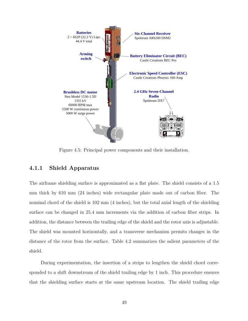
2.4 GHz Seven-Channel
RadioSpektrum DX7
Electronic Speed Controller (ESC)Castle Creations Phoenix 160-Amp
Arming
switch
Six-Channel ReceiverSpektrum AR6200 DSM2
Batteries2 × 6S2P (22.2 V) Lipo
44.4 V total
Brushless DC motorNeu Model 1530-1.5D
1355 kV
60000 RPM max
2500 W continuous power
5000 W surge power
Battery Eliminator Circuit (BEC)Castle Creations BEC Pro
Figure 4.5: Principal power components and their installation.
4.1.1 Shield Apparatus
The airframe shielding surface is approximated as a flat plate. The shield consists of a 1.5
mm thick by 610 mm (24 inches) wide rectangular plate made out of carbon fiber. The
nominal chord of the shield is 102 mm (4 inches), but the total axial length of the shielding
surface can be changed in 25.4 mm increments via the addition of carbon fiber strips. In
addition, the distance between the trailing edge of the shield and the rotor axis is adjustable.
The shield was mounted horizontally, and a transverse mechanism permits changes in the
distance of the rotor from the surface. Table 4.2 summarizes the salient parameters of the
shield.
During experimentation, the insertion of a strips to lengthen the shield chord corre-
sponded to a shift downstream of the shield trailing edge by 1 inch. This procedure ensures
that the shielding surface starts at the same upstream location. The shield trailing edge
49
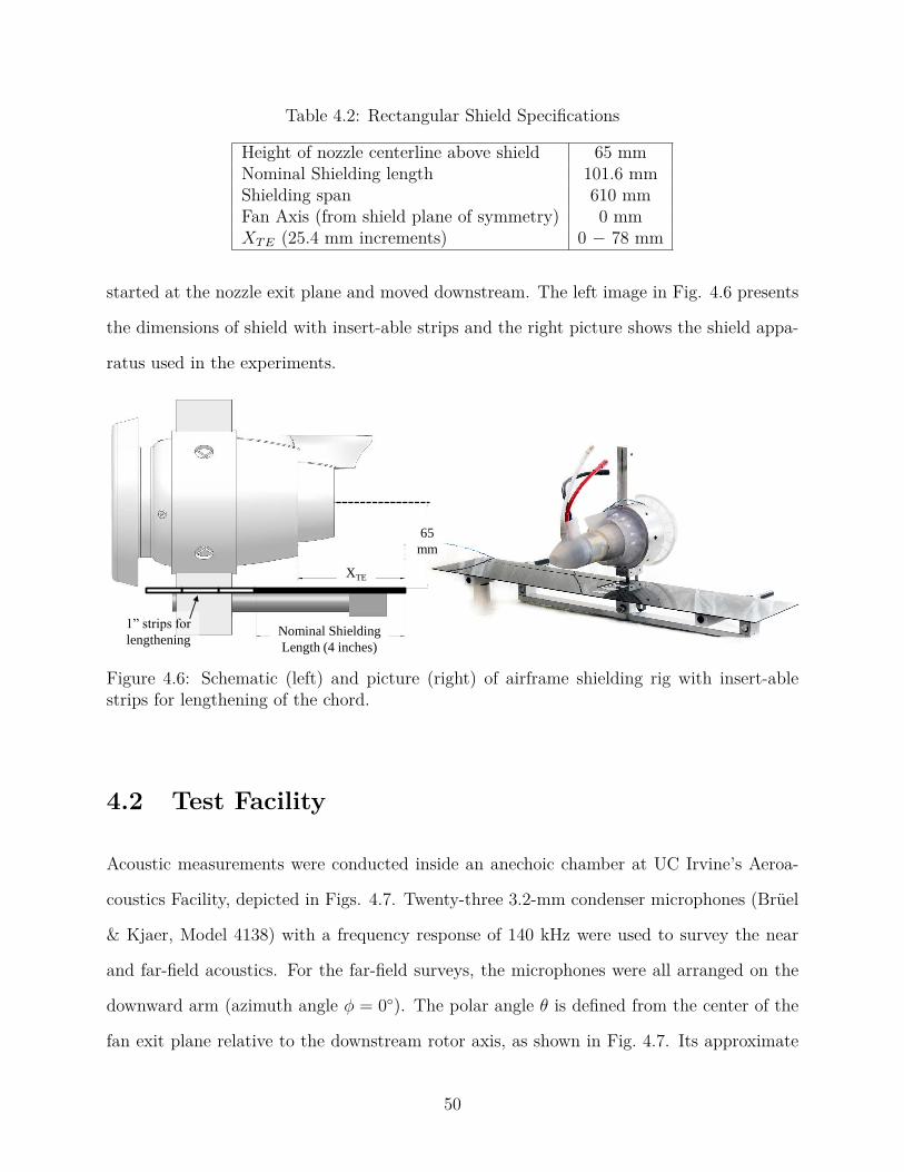
Table 4.2: Rectangular Shield Specifications
Height of nozzle centerline above shield 65 mmNominal Shielding length 101.6 mmShielding span 610 mmFan Axis (from shield plane of symmetry) 0 mmXTE (25.4 mm increments) 0 − 78 mm
started at the nozzle exit plane and moved downstream. The left image in Fig. 4.6 presents
the dimensions of shield with insert-able strips and the right picture shows the shield appa-
ratus used in the experiments.
Nominal Shielding
Length (4 inches)
XTE
1” strips for
lengthening
65
mm
Figure 4.6: Schematic (left) and picture (right) of airframe shielding rig with insert-ablestrips for lengthening of the chord.
4.2 Test Facility
Acoustic measurements were conducted inside an anechoic chamber at UC Irvine’s Aeroa-
coustics Facility, depicted in Figs. 4.7. Twenty-three 3.2-mm condenser microphones (Brüel
& Kjaer, Model 4138) with a frequency response of 140 kHz were used to survey the near
and far-field acoustics. For the far-field surveys, the microphones were all arranged on the
downward arm (azimuth angle φ = 0). The polar angle θ is defined from the center of the
fan exit plane relative to the downstream rotor axis, as shown in Fig. 4.7. Its approximate
50
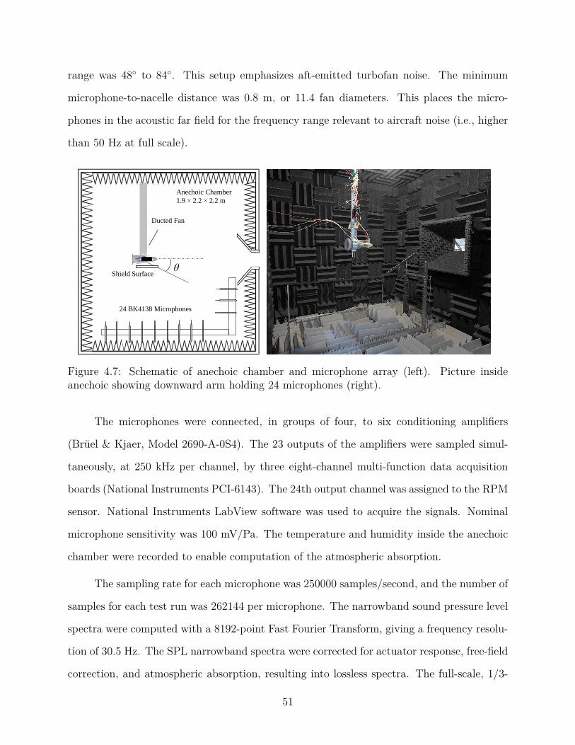
range was 48 to 84. This setup emphasizes aft-emitted turbofan noise. The minimum
microphone-to-nacelle distance was 0.8 m, or 11.4 fan diameters. This places the micro-
phones in the acoustic far field for the frequency range relevant to aircraft noise (i.e., higher
than 50 Hz at full scale).
Ducted Fan
θ
24 BK4138 Microphones
Anechoic Chamber
1.9 × 2.2 × 2.2 m
Shield Surface
Figure 4.7: Schematic of anechoic chamber and microphone array (left). Picture insideanechoic showing downward arm holding 24 microphones (right).
The microphones were connected, in groups of four, to six conditioning amplifiers
(Brüel & Kjaer, Model 2690-A-0S4). The 23 outputs of the amplifiers were sampled simul-
taneously, at 250 kHz per channel, by three eight-channel multi-function data acquisition
boards (National Instruments PCI-6143). The 24th output channel was assigned to the RPM
sensor. National Instruments LabView software was used to acquire the signals. Nominal
microphone sensitivity was 100 mV/Pa. The temperature and humidity inside the anechoic
chamber were recorded to enable computation of the atmospheric absorption.
The sampling rate for each microphone was 250000 samples/second, and the number of
samples for each test run was 262144 per microphone. The narrowband sound pressure level
spectra were computed with a 8192-point Fast Fourier Transform, giving a frequency resolu-
tion of 30.5 Hz. The SPL narrowband spectra were corrected for actuator response, free-field
correction, and atmospheric absorption, resulting into lossless spectra. The full-scale, 1/3-
51
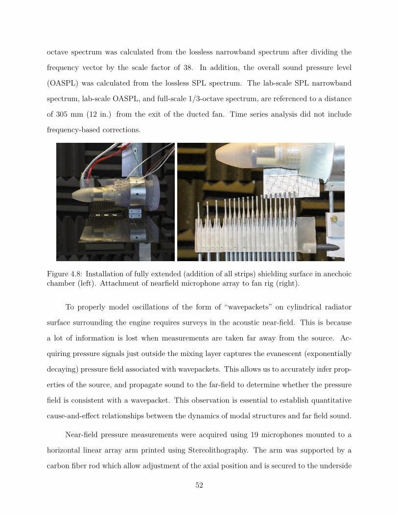
octave spectrum was calculated from the lossless narrowband spectrum after dividing the
frequency vector by the scale factor of 38. In addition, the overall sound pressure level
(OASPL) was calculated from the lossless SPL spectrum. The lab-scale SPL narrowband
spectrum, lab-scale OASPL, and full-scale 1/3-octave spectrum, are referenced to a distance
of 305 mm (12 in.) from the exit of the ducted fan. Time series analysis did not include
frequency-based corrections.
Figure 4.8: Installation of fully extended (addition of all strips) shielding surface in anechoicchamber (left). Attachment of nearfield microphone array to fan rig (right).
To properly model oscillations of the form of “wavepackets” on cylindrical radiator
surface surrounding the engine requires surveys in the acoustic near-field. This is because
a lot of information is lost when measurements are taken far away from the source. Ac-
quiring pressure signals just outside the mixing layer captures the evanescent (exponentially
decaying) pressure field associated with wavepackets. This allows us to accurately infer prop-
erties of the source, and propagate sound to the far-field to determine whether the pressure
field is consistent with a wavepacket. This observation is essential to establish quantitative
cause-and-effect relationships between the dynamics of modal structures and far field sound.
Near-field pressure measurements were acquired using 19 microphones mounted to a
horizontal linear array arm printed using Stereolithography. The arm was supported by a
carbon fiber rod which allow adjustment of the axial position and is secured to the underside
52
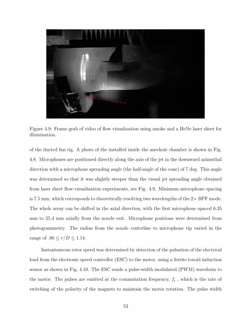
Figure 4.9: Frame grab of video of flow visualization using smoke and a HeNe laser sheet forillumination.
of the ducted fan rig. A photo of the installed inside the anechoic chamber is shown in Fig.
4.8. Microphones are positioned directly along the axis of the jet in the downward azimuthal
direction with a microphone spreading angle (the half-angle of the cone) of 7 deg. This angle
was determined so that it was slightly steeper than the visual jet spreading angle obtained
from laser sheet flow-visualization experiments, see Fig. 4.9. Minimum microphone spacing
is 7.5 mm, which corresponds to theoretically resolving two wavelengths of the 2× BPF mode.
The whole array can be shifted in the axial direction, with the first microphone spaced 6.35
mm to 25.4 mm axially from the nozzle exit. Microphone positions were determined from
photogrammetry. The radius from the nozzle centerline to microphone tip varied in the
range of .86 ≤ r/D ≤ 1.14.
Instantaneous rotor speed was determined by detection of the pulsation of the electrical
load from the electronic speed controller (ESC) to the motor, using a ferrite toroid induction
sensor as shown in Fig. 4.10. The ESC sends a pulse-width modulated (PWM) waveform to
the motor. The pulses are emitted at the commutation frequency, fc , which is the rate of
switching of the polarity of the magnets to maintain the motor rotation. The pulse width
53
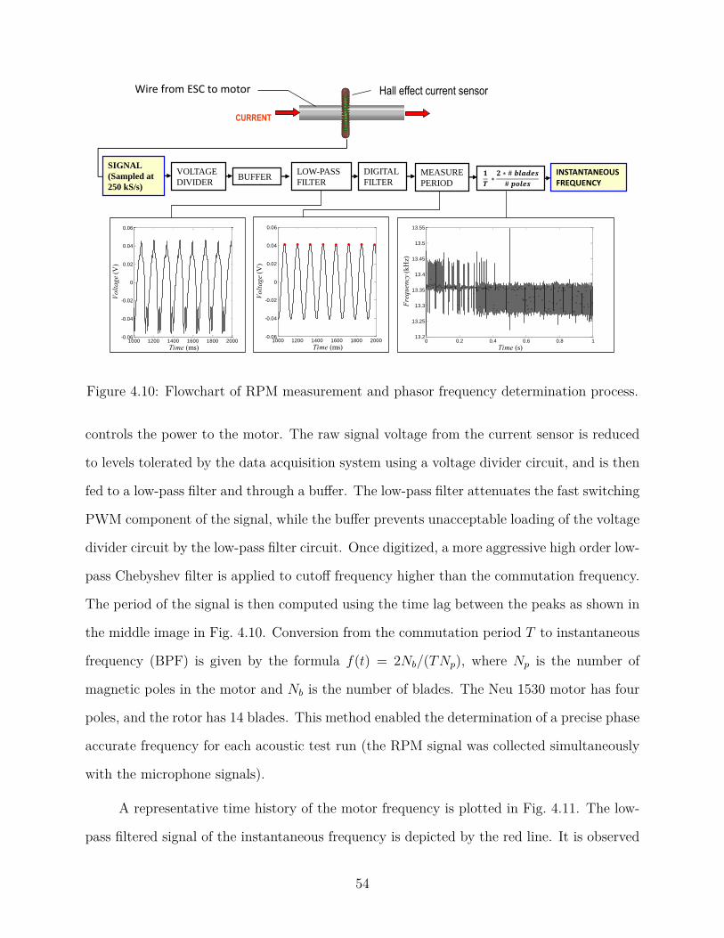
VOLTAGE
DIVIDER BUFFER
LOW-PASS
FILTER
DIGITAL
FILTER
Hall effect current sensor Wire from ESC to motor
CURRENT
MEASURE
PERIOD
𝟏
𝑻 ∗
𝟐 ∗ # 𝒃𝒍𝒂𝒅𝒆𝒔
# 𝒑𝒐𝒍𝒆𝒔
INSTANTANEOUS FREQUENCY
SIGNAL
(Sampled at
250 kS/s)
1000 1200 1400 1600 1800 2000-0.06
-0.04
-0.02
0
0.02
0.04
0.06
Time (ms)
Vo
lta
ge
(V)
1000 1200 1400 1600 1800 2000-0.06
-0.04
-0.02
0
0.02
0.04
0.06
Time (ms)
Vo
lta
ge
(V)
0 0.2 0.4 0.6 0.8 113.2
13.25
13.3
13.35
13.4
13.45
13.5
13.55
Time (s)
Fre
qu
ency
(k
Hz)
Figure 4.10: Flowchart of RPM measurement and phasor frequency determination process.
controls the power to the motor. The raw signal voltage from the current sensor is reduced
to levels tolerated by the data acquisition system using a voltage divider circuit, and is then
fed to a low-pass filter and through a buffer. The low-pass filter attenuates the fast switching
PWM component of the signal, while the buffer prevents unacceptable loading of the voltage
divider circuit by the low-pass filter circuit. Once digitized, a more aggressive high order low-
pass Chebyshev filter is applied to cutoff frequency higher than the commutation frequency.
The period of the signal is then computed using the time lag between the peaks as shown in
the middle image in Fig. 4.10. Conversion from the commutation period T to instantaneous
frequency (BPF) is given by the formula f(t) = 2Nb/(TNp), where Np is the number of
magnetic poles in the motor and Nb is the number of blades. The Neu 1530 motor has four
poles, and the rotor has 14 blades. This method enabled the determination of a precise phase
accurate frequency for each acoustic test run (the RPM signal was collected simultaneously
with the microphone signals).
A representative time history of the motor frequency is plotted in Fig. 4.11. The low-
pass filtered signal of the instantaneous frequency is depicted by the red line. It is observed
54
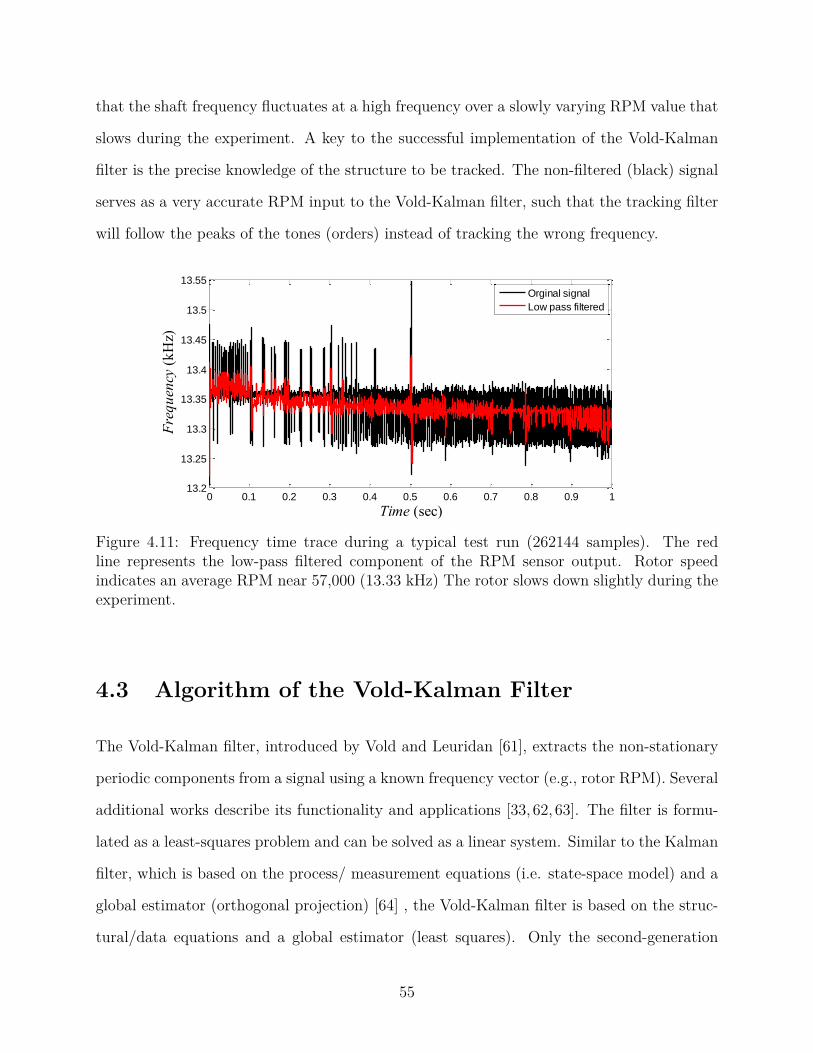
that the shaft frequency fluctuates at a high frequency over a slowly varying RPM value that
slows during the experiment. A key to the successful implementation of the Vold-Kalman
filter is the precise knowledge of the structure to be tracked. The non-filtered (black) signal
serves as a very accurate RPM input to the Vold-Kalman filter, such that the tracking filter
will follow the peaks of the tones (orders) instead of tracking the wrong frequency.
0 0.1 0.2 0.3 0.4 0.5 0.6 0.7 0.8 0.9 113.2
13.25
13.3
13.35
13.4
13.45
13.5
13.55
Time (sec)
Fre
qu
ency
(k
Hz)
Orginal signal
Low pass filtered
Figure 4.11: Frequency time trace during a typical test run (262144 samples). The redline represents the low-pass filtered component of the RPM sensor output. Rotor speedindicates an average RPM near 57,000 (13.33 kHz) The rotor slows down slightly during theexperiment.
4.3 Algorithm of the Vold-Kalman Filter
The Vold-Kalman filter, introduced by Vold and Leuridan [61], extracts the non-stationary
periodic components from a signal using a known frequency vector (e.g., rotor RPM). Several
additional works describe its functionality and applications [33, 62, 63]. The filter is formu-
lated as a least-squares problem and can be solved as a linear system. Similar to the Kalman
filter, which is based on the process/ measurement equations (i.e. state-space model) and a
global estimator (orthogonal projection) [64] , the Vold-Kalman filter is based on the struc-
tural/data equations and a global estimator (least squares). Only the second-generation
55
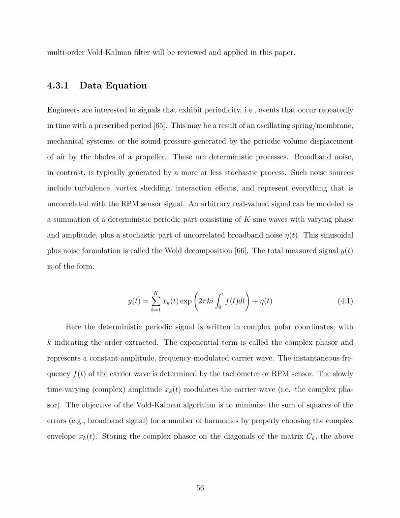
multi-order Vold-Kalman filter will be reviewed and applied in this paper.
4.3.1 Data Equation
Engineers are interested in signals that exhibit periodicity, i.e., events that occur repeatedly
in time with a prescribed period [65]. This may be a result of an oscillating spring/membrane,
mechanical systems, or the sound pressure generated by the periodic volume displacement
of air by the blades of a propeller. These are deterministic processes. Broadband noise,
in contrast, is typically generated by a more or less stochastic process. Such noise sources
include turbulence, vortex shedding, interaction effects, and represent everything that is
uncorrelated with the RPM sensor signal. An arbitrary real-valued signal can be modeled as
a summation of a deterministic periodic part consisting of K sine waves with varying phase
and amplitude, plus a stochastic part of uncorrelated broadband noise η(t). This sinusoidal
plus noise formulation is called the Wold decomposition [66]. The total measured signal y(t)
is of the form:
y(t) =K∑k=1
xk(t) exp(
2πki∫ t
0f(t)dt
)+ η(t) (4.1)
Here the deterministic periodic signal is written in complex polar coordinates, with
k indicating the order extracted. The exponential term is called the complex phasor and
represents a constant-amplitude, frequency-modulated carrier wave. The instantaneous fre-
quency f(t) of the carrier wave is determined by the tachometer or RPM sensor. The slowly
time-varying (complex) amplitude xk(t) modulates the carrier wave (i.e. the complex pha-
sor). The objective of the Vold-Kalman algorithm is to minimize the sum of squares of the
errors (e.g., broadband signal) for a number of harmonics by properly choosing the complex
envelope xk(t). Storing the complex phasor on the diagonals of the matrix Ck, the above
56

expression takes the compact form:
y(t)−K∑k=1
Ckxk(t) = η(t) (4.2)
4.3.2 Structural Equation
The structural equation imposes smoothness on the complex envelope xk(t) by means of
a backward finite-difference sequence. This is accomplished by minimizing the error ε(t)
made in the smoothness of the envelope, where the smoothness is represented by a low-order
polynomial. The polynomial order designates the number of the filter poles. The equations
for 1-,2-, and 3- pole filter coefficients are found by the Pascal triangle:
∇xk[n] = xk[n]− xk[n− 1] = εk[n] (4.3a)
∇2xk[n] = xk[n]− 2xk[n− 1] + xk[n− 2] = εk[n] (4.3b)
∇3xk[n] = xk[n]− 3xk[n− 1] + 3xk[n− 2]− xk[n− 3] = εk[n] (4.3c)
Assuming a second-order difference, the system of structural equations with the complex
envelope xk for order k as the unknown takes the form of a matrix equation:
1 −2 1 0 · · ·
0 1 −2 1 0 · · ·... 0 1 −2 1 0 · · ·
... 0 . . . . . . . . . 0 · · ·
1 −2 1 0
0 0 0 0 1 −2 1
xk[1]
xk[2]
xk[3]...
xk[n]
=
εk[3]
εk[4]
εk[5]...
εk[n]
(4.4)
57
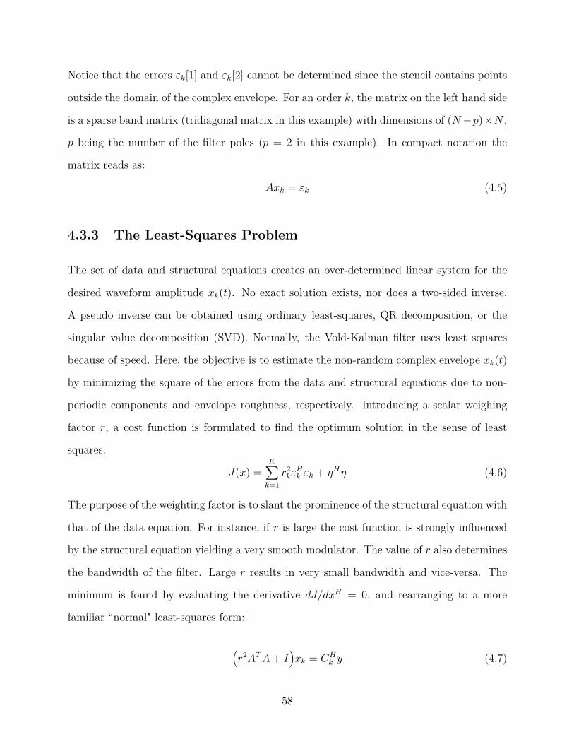
Notice that the errors εk[1] and εk[2] cannot be determined since the stencil contains points
outside the domain of the complex envelope. For an order k, the matrix on the left hand side
is a sparse band matrix (tridiagonal matrix in this example) with dimensions of (N−p)×N ,
p being the number of the filter poles (p = 2 in this example). In compact notation the
matrix reads as:
Axk = εk (4.5)
4.3.3 The Least-Squares Problem
The set of data and structural equations creates an over-determined linear system for the
desired waveform amplitude xk(t). No exact solution exists, nor does a two-sided inverse.
A pseudo inverse can be obtained using ordinary least-squares, QR decomposition, or the
singular value decomposition (SVD). Normally, the Vold-Kalman filter uses least squares
because of speed. Here, the objective is to estimate the non-random complex envelope xk(t)
by minimizing the square of the errors from the data and structural equations due to non-
periodic components and envelope roughness, respectively. Introducing a scalar weighing
factor r, a cost function is formulated to find the optimum solution in the sense of least
squares:
J(x) =K∑k=1
r2kεHk εk + ηHη (4.6)
The purpose of the weighting factor is to slant the prominence of the structural equation with
that of the data equation. For instance, if r is large the cost function is strongly influenced
by the structural equation yielding a very smooth modulator. The value of r also determines
the bandwidth of the filter. Large r results in very small bandwidth and vice-versa. The
minimum is found by evaluating the derivative dJ/dxH = 0, and rearranging to a more
familiar “normal" least-squares form:
(r2ATA+ I
)xk = CH
k y (4.7)
58
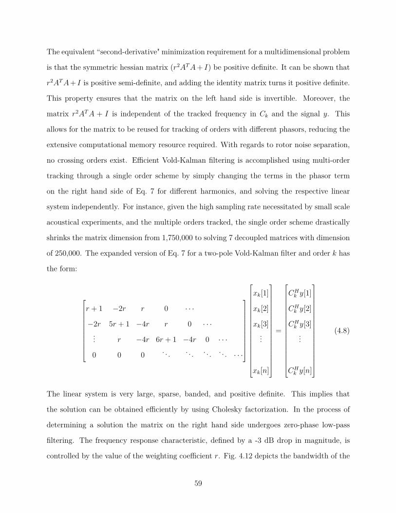
The equivalent “second-derivative" minimization requirement for a multidimensional problem
is that the symmetric hessian matrix (r2ATA+ I) be positive definite. It can be shown that
r2ATA+ I is positive semi-definite, and adding the identity matrix turns it positive definite.
This property ensures that the matrix on the left hand side is invertible. Moreover, the
matrix r2ATA + I is independent of the tracked frequency in Ck and the signal y. This
allows for the matrix to be reused for tracking of orders with different phasors, reducing the
extensive computational memory resource required. With regards to rotor noise separation,
no crossing orders exist. Efficient Vold-Kalman filtering is accomplished using multi-order
tracking through a single order scheme by simply changing the terms in the phasor term
on the right hand side of Eq. 7 for different harmonics, and solving the respective linear
system independently. For instance, given the high sampling rate necessitated by small scale
acoustical experiments, and the multiple orders tracked, the single order scheme drastically
shrinks the matrix dimension from 1,750,000 to solving 7 decoupled matrices with dimension
of 250,000. The expanded version of Eq. 7 for a two-pole Vold-Kalman filter and order k has
the form:
r + 1 −2r r 0 · · ·
−2r 5r + 1 −4r r 0 · · ·... r −4r 6r + 1 −4r 0 · · ·
0 0 0 . . . . . . . . . . . . · · ·
xk[1]
xk[2]
xk[3]...
xk[n]
=
CHk y[1]
CHk y[2]
CHk y[3]...
CHk y[n]
(4.8)
The linear system is very large, sparse, banded, and positive definite. This implies that
the solution can be obtained efficiently by using Cholesky factorization. In the process of
determining a solution the matrix on the right hand side undergoes zero-phase low-pass
filtering. The frequency response characteristic, defined by a -3 dB drop in magnitude, is
controlled by the value of the weighting coefficient r. Fig. 4.12 depicts the bandwidth of the
59
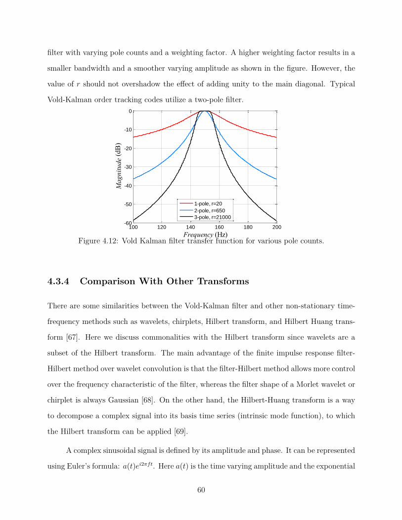
filter with varying pole counts and a weighting factor. A higher weighting factor results in a
smaller bandwidth and a smoother varying amplitude as shown in the figure. However, the
value of r should not overshadow the effect of adding unity to the main diagonal. Typical
Vold-Kalman order tracking codes utilize a two-pole filter.
100 120 140 160 180 200-60
-50
-40
-30
-20
-10
0
Frequency (Hz)
Ma
gn
itu
de
(dB
)
1-pole, r=20
2-pole, r=650
3-pole, r=21000
Figure 4.12: Vold Kalman filter transfer function for various pole counts.
4.3.4 Comparison With Other Transforms
There are some similarities between the Vold-Kalman filter and other non-stationary time-
frequency methods such as wavelets, chirplets, Hilbert transform, and Hilbert Huang trans-
form [67]. Here we discuss commonalities with the Hilbert transform since wavelets are a
subset of the Hilbert transform. The main advantage of the finite impulse response filter-
Hilbert method over wavelet convolution is that the filter-Hilbert method allows more control
over the frequency characteristic of the filter, whereas the filter shape of a Morlet wavelet or
chirplet is always Gaussian [68]. On the other hand, the Hilbert-Huang transform is a way
to decompose a complex signal into its basis time series (intrinsic mode function), to which
the Hilbert transform can be applied [69].
A complex sinusoidal signal is defined by its amplitude and phase. It can be represented
using Euler’s formula: a(t)ei2πft. Here a(t) is the time varying amplitude and the exponential
60
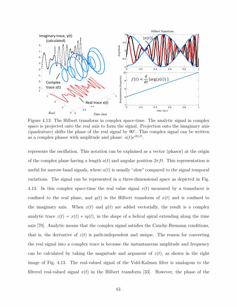
0
0.2
0.4
0.6
0.8
1
-2
-1
0
1
2
-2
-1.5
-1
-0.5
0
0.5
1
1.5
2
Time (ms)Real
Ima
gin
ary
0 0.2 0.4 0.6 0.8 1-1
-0.5
0
0.5
1
Am
plitu
de
Hilbert Transform
0 0.2 0.4 0.6 0.8 12
4
6
8
10
Inst
an
tan
eou
s fr
equ
ency
time (sec)
Real trace x(t)
Imaginary trace, y(t) (calculated)
Complex trace z(t)
𝑧(𝑡)
𝑓 𝑡 =𝑑
𝑑𝑡arg(𝑧 𝑡 )
Figure 4.13: The Hilbert transform in complex space-time. The analytic signal in complexspace is projected onto the real axis to form the signal. Projection onto the imaginary axis(quadrature) shifts the phase of the real signal by 90. This complex signal can be writtenas a complex phasor with amplitude and phase: a(t)ei2πft.
represents the oscillation. This notation can be explained as a vector (phasor) at the origin
of the complex plane having a length a(t) and angular position 2πft. This representation is
useful for narrow-band signals, where a(t) is usually “slow" compared to the signal temporal
variations. The signal can be represented in a three-dimensional space as depicted in Fig.
4.13. In this complex space-time the real value signal x(t) measured by a transducer is
confined to the real plane, and y(t) is the Hilbert transform of x(t) and is confined to
the imaginary axis. When x(t) and y(t) are added vectorially, the result is a complex
analytic trace z(t) = x(t) + iy(t), in the shape of a helical spiral extending along the time
axis [70]. Analytic means that the complex signal satisfies the Cauchy-Riemann conditions,
that is, the derivative of z(t) is path-independent and unique. The reason for converting
the real signal into a complex trace is because the instantaneous amplitude and frequency
can be calculated by taking the magnitude and argument of z(t), as shown in the right
image of Fig. 4.13. The real-valued signal of the Vold-Kalman filter is analogous to the
filtered real-valued signal x(t) in the Hilbert transform [33]. However, the phase of the
61
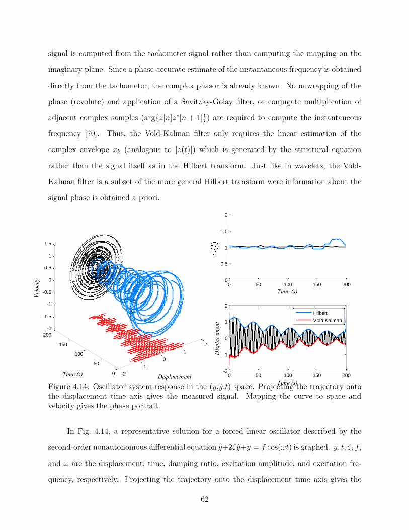
signal is computed from the tachometer signal rather than computing the mapping on the
imaginary plane. Since a phase-accurate estimate of the instantaneous frequency is obtained
directly from the tachometer, the complex phasor is already known. No unwrapping of the
phase (revolute) and application of a Savitzky-Golay filter, or conjugate multiplication of
adjacent complex samples (argz[n]z∗[n + 1]) are required to compute the instantaneous
frequency [70]. Thus, the Vold-Kalman filter only requires the linear estimation of the
complex envelope xk (analogous to |z(t)|) which is generated by the structural equation
rather than the signal itself as in the Hilbert transform. Just like in wavelets, the Vold-
Kalman filter is a subset of the more general Hilbert transform were information about the
signal phase is obtained a priori.
-2
-1
0
1
2
0
50
100
150
200
-2
-1.5
-1
-0.5
0
0.5
1
1.5
DisplacementTime (s)
Vel
oci
ty
0 50 100 150 2000
0.5
1
1.5
2
Time (s)
0 50 100 150 200-2
-1
0
1
2
Time (s)
Dis
pla
cem
ent
Hilbert
Vold Kalman
Figure 4.14: Oscillator system response in the (y,y,t) space. Projecting the trajectory ontothe displacement time axis gives the measured signal. Mapping the curve to space andvelocity gives the phase portrait.
In Fig. 4.14, a representative solution for a forced linear oscillator described by the
second-order nonautonomous differential equation y+2ζy+y = f cos(ωt) is graphed. y, t, ζ, f,
and ω are the displacement, time, damping ratio, excitation amplitude, and excitation fre-
quency, respectively. Projecting the trajectory onto the displacement time axis gives the
62
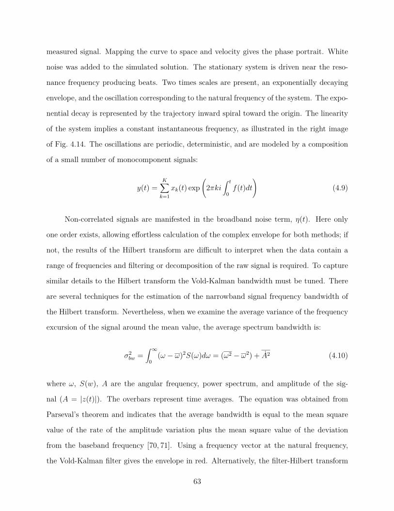
measured signal. Mapping the curve to space and velocity gives the phase portrait. White
noise was added to the simulated solution. The stationary system is driven near the reso-
nance frequency producing beats. Two times scales are present, an exponentially decaying
envelope, and the oscillation corresponding to the natural frequency of the system. The expo-
nential decay is represented by the trajectory inward spiral toward the origin. The linearity
of the system implies a constant instantaneous frequency, as illustrated in the right image
of Fig. 4.14. The oscillations are periodic, deterministic, and are modeled by a composition
of a small number of monocomponent signals:
y(t) =K∑k=1
xk(t) exp(
2πki∫ t
0f(t)dt
)(4.9)
Non-correlated signals are manifested in the broadband noise term, η(t). Here only
one order exists, allowing effortless calculation of the complex envelope for both methods; if
not, the results of the Hilbert transform are difficult to interpret when the data contain a
range of frequencies and filtering or decomposition of the raw signal is required. To capture
similar details to the Hilbert transform the Vold-Kalman bandwidth must be tuned. There
are several techniques for the estimation of the narrowband signal frequency bandwidth of
the Hilbert transform. Nevertheless, when we examine the average variance of the frequency
excursion of the signal around the mean value, the average spectrum bandwidth is:
σ2bw =
∫ ∞0
(ω − ω)2S(ω)dω = (ω2 − ω2) + A2 (4.10)
where ω, S(w), A are the angular frequency, power spectrum, and amplitude of the sig-
nal (A = |z(t)|). The overbars represent time averages. The equation was obtained from
Parseval’s theorem and indicates that the average bandwidth is equal to the mean square
value of the rate of the amplitude variation plus the mean square value of the deviation
from the baseband frequency [70, 71]. Using a frequency vector at the natural frequency,
the Vold-Kalman filter gives the envelope in red. Alternatively, the filter-Hilbert transform
63
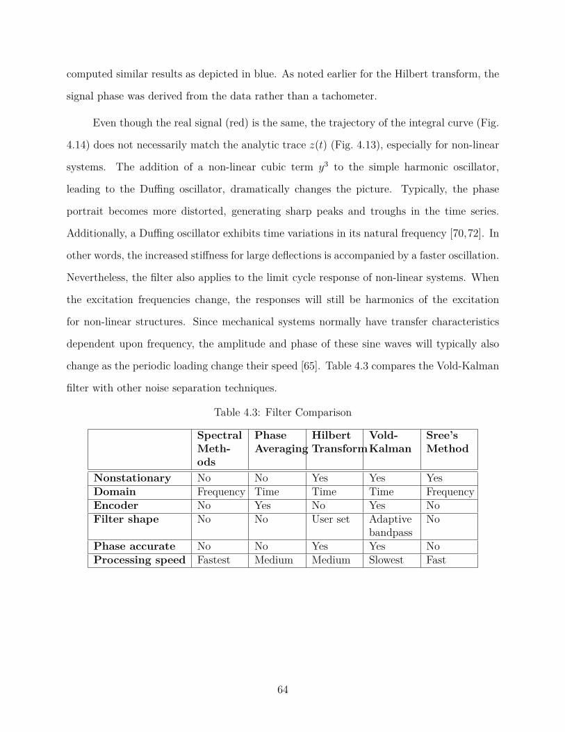
computed similar results as depicted in blue. As noted earlier for the Hilbert transform, the
signal phase was derived from the data rather than a tachometer.
Even though the real signal (red) is the same, the trajectory of the integral curve (Fig.
4.14) does not necessarily match the analytic trace z(t) (Fig. 4.13), especially for non-linear
systems. The addition of a non-linear cubic term y3 to the simple harmonic oscillator,
leading to the Duffing oscillator, dramatically changes the picture. Typically, the phase
portrait becomes more distorted, generating sharp peaks and troughs in the time series.
Additionally, a Duffing oscillator exhibits time variations in its natural frequency [70,72]. In
other words, the increased stiffness for large deflections is accompanied by a faster oscillation.
Nevertheless, the filter also applies to the limit cycle response of non-linear systems. When
the excitation frequencies change, the responses will still be harmonics of the excitation
for non-linear structures. Since mechanical systems normally have transfer characteristics
dependent upon frequency, the amplitude and phase of these sine waves will typically also
change as the periodic loading change their speed [65]. Table 4.3 compares the Vold-Kalman
filter with other noise separation techniques.
Table 4.3: Filter Comparison
SpectralMeth-ods
PhaseAveraging
HilbertTransform
Vold-Kalman
Sree’sMethod
Nonstationary No No Yes Yes YesDomain Frequency Time Time Time FrequencyEncoder No Yes No Yes NoFilter shape No No User set Adaptive
bandpassNo
Phase accurate No No Yes Yes NoProcessing speed Fastest Medium Medium Slowest Fast
64

5
Cha
pter
Results and Discussion
For all the conditions covered in this report, the RPM was 56500 ± 1.0 %. This
corresponds to a rotor tip Mach number of 0.61 ± 1.0 %. Fan exhaust total pressure
was 2.30 psig, which translates to FPR=1.157, rotor induced velocity of 88.9 m/s, fan exit
velocity of 159 m/s, and power output of 4700 W (6.3 hp). This translates to a motor
conversion efficiency of 92 % according to ESC data logs.
A two-pole second-generation, multi-order using single order scheme Vold-Kalman filter
was used to isolate each harmonic from a narrow frequency band around the tracked tone
while preserving accurate phase information. To work out the phasor information in the
data equation, the tracked tone was determined by the instantaneous frequency of the rotor
specified by the RPM sensor. Although the signal consists of a rapidly changing frequency,
the Vold-Kalman filter is able to track even at extreme slew rates. Filtering of the 23
microphone data for 6 orders took a few minutes on an Intel Xenon based desktop computer
using the Matlab® backslash matrix solver. No down-sampling was applied. The acoustic
results will be presented as follows:
1. Isolated ducted fan time history, plotted for various polar angles, referenced to 305-mm
arc.
2. Isolated ducted fan narrowband SPL spectra in laboratory scale, referenced to 305-mm
65
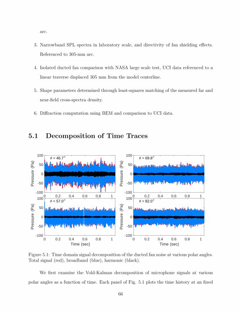
arc.
3. Narrowband SPL spectra in laboratory scale, and directivity of fan shielding effects.
Referenced to 305-mm arc.
4. Isolated ducted fan comparison with NASA large scale test, UCI data referenced to a
linear traverse displaced 305 mm from the model centerline.
5. Shape parameters determined through least-squares matching of the measured far and
near-field cross-spectra density.
6. Diffraction computation using BEM and comparison to UCI data.
5.1 Decomposition of Time Traces
0 0.2 0.4 0.6 0.8 1-100
-50
0
50
100
Pre
ssur
e (
Pa)
= 46.7ø
0 0.2 0.4 0.6 0.8 1 Time (sec)
-100
-50
0
50
100
Pre
ssur
e (
Pa)
= 57.0ø 0 0.2 0.4 0.6 0.8 1
-100
-50
0
50
100
Pre
ssur
e (
Pa)
= 69.8ø
0 0.2 0.4 0.6 0.8 1 Time (sec)
-100
-50
0
50
100
Pre
ssur
e (
Pa)
= 82.0ø
Figure 5.1: Time domain signal decomposition of the ducted fan noise at various polar angles.Total signal (red), broadband (blue), harmonic (black).
We first examine the Vold-Kalman decomposition of microphone signals at various
polar angles as a function of time. Each panel of Fig. 5.1 plots the time history at an fixed
66
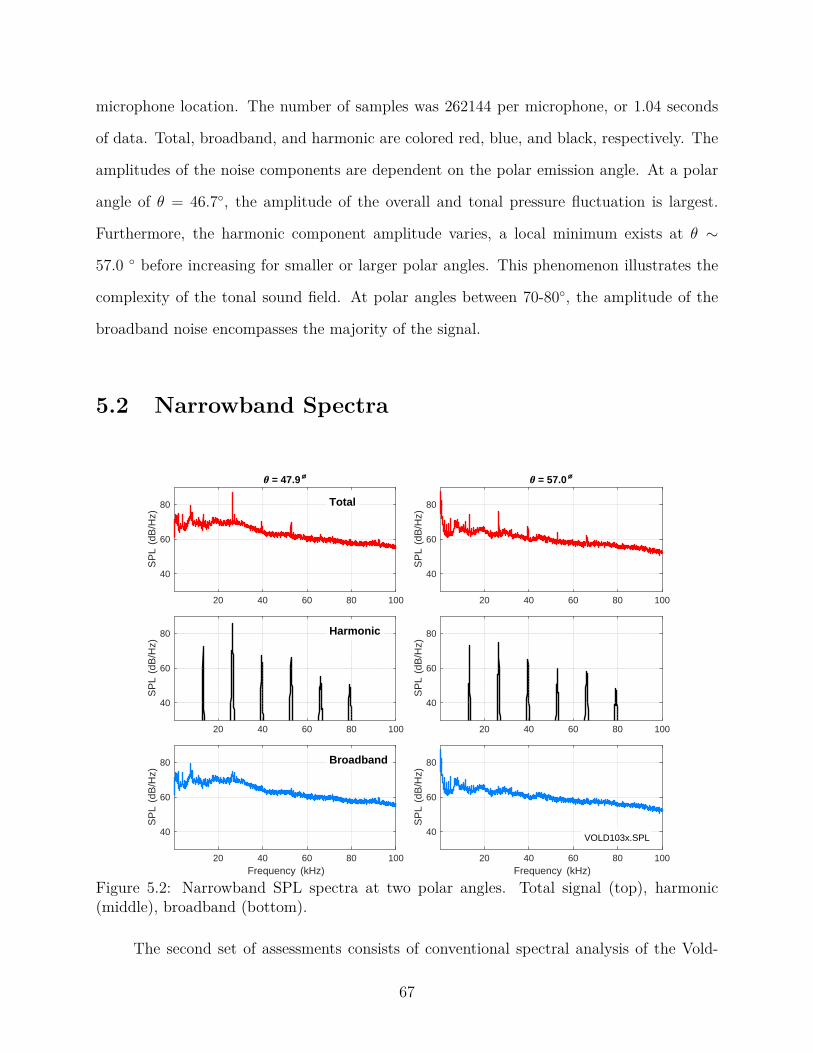
microphone location. The number of samples was 262144 per microphone, or 1.04 seconds
of data. Total, broadband, and harmonic are colored red, blue, and black, respectively. The
amplitudes of the noise components are dependent on the polar emission angle. At a polar
angle of θ = 46.7, the amplitude of the overall and tonal pressure fluctuation is largest.
Furthermore, the harmonic component amplitude varies, a local minimum exists at θ ∼
57.0 before increasing for smaller or larger polar angles. This phenomenon illustrates the
complexity of the tonal sound field. At polar angles between 70-80, the amplitude of the
broadband noise encompasses the majority of the signal.
5.2 Narrowband Spectra
20 40 60 80 100
40
60
80
SP
L (
dB/H
z)
= 47.9ø
Total
20 40 60 80 100
40
60
80
SP
L (
dB/H
z)
= 57.0ø
20 40 60 80 100
40
60
80
SP
L (
dB/H
z)
Harmonic
20 40 60 80 100
40
60
80
SP
L (
dB/H
z)
20 40 60 80 100 Frequency (kHz)
40
60
80
SP
L (
dB/H
z)
Broadband
20 40 60 80 100 Frequency (kHz)
40
60
80
SP
L (
dB/H
z)
VOLD103x.SPL
Figure 5.2: Narrowband SPL spectra at two polar angles. Total signal (top), harmonic(middle), broadband (bottom).
The second set of assessments consists of conventional spectral analysis of the Vold-
67
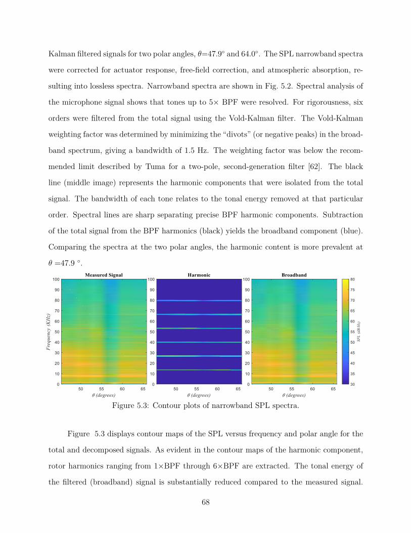
Kalman filtered signals for two polar angles, θ=47.9 and 64.0. The SPL narrowband spectra
were corrected for actuator response, free-field correction, and atmospheric absorption, re-
sulting into lossless spectra. Narrowband spectra are shown in Fig. 5.2. Spectral analysis of
the microphone signal shows that tones up to 5× BPF were resolved. For rigorousness, six
orders were filtered from the total signal using the Vold-Kalman filter. The Vold-Kalman
weighting factor was determined by minimizing the “divots” (or negative peaks) in the broad-
band spectrum, giving a bandwidth of 1.5 Hz. The weighting factor was below the recom-
mended limit described by Tuma for a two-pole, second-generation filter [62]. The black
line (middle image) represents the harmonic components that were isolated from the total
signal. The bandwidth of each tone relates to the tonal energy removed at that particular
order. Spectral lines are sharp separating precise BPF harmonic components. Subtraction
of the total signal from the BPF harmonics (black) yields the broadband component (blue).
Comparing the spectra at the two polar angles, the harmonic content is more prevalent at
θ =47.9 .
Figure 5.3: Contour plots of narrowband SPL spectra.
Figure 5.3 displays contour maps of the SPL versus frequency and polar angle for the
total and decomposed signals. As evident in the contour maps of the harmonic component,
rotor harmonics ranging from 1×BPF through 6×BPF are extracted. The tonal energy of
the filtered (broadband) signal is substantially reduced compared to the measured signal.
68
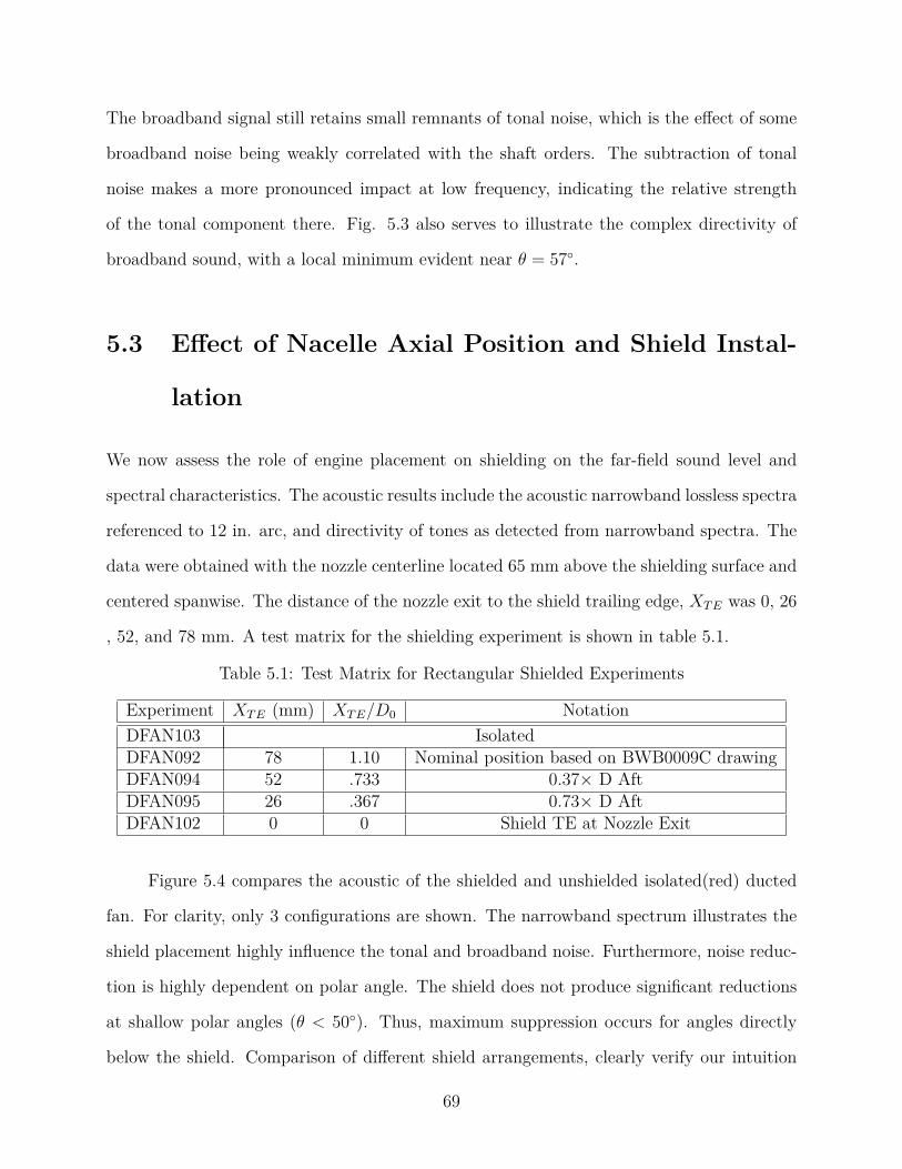
The broadband signal still retains small remnants of tonal noise, which is the effect of some
broadband noise being weakly correlated with the shaft orders. The subtraction of tonal
noise makes a more pronounced impact at low frequency, indicating the relative strength
of the tonal component there. Fig. 5.3 also serves to illustrate the complex directivity of
broadband sound, with a local minimum evident near θ = 57.
5.3 Effect of Nacelle Axial Position and Shield Instal-
lation
We now assess the role of engine placement on shielding on the far-field sound level and
spectral characteristics. The acoustic results include the acoustic narrowband lossless spectra
referenced to 12 in. arc, and directivity of tones as detected from narrowband spectra. The
data were obtained with the nozzle centerline located 65 mm above the shielding surface and
centered spanwise. The distance of the nozzle exit to the shield trailing edge, XTE was 0, 26
, 52, and 78 mm. A test matrix for the shielding experiment is shown in table 5.1.
Table 5.1: Test Matrix for Rectangular Shielded Experiments
Experiment XTE (mm) XTE/D0 NotationDFAN103 IsolatedDFAN092 78 1.10 Nominal position based on BWB0009C drawingDFAN094 52 .733 0.37× D AftDFAN095 26 .367 0.73× D AftDFAN102 0 0 Shield TE at Nozzle Exit
Figure 5.4 compares the acoustic of the shielded and unshielded isolated(red) ducted
fan. For clarity, only 3 configurations are shown. The narrowband spectrum illustrates the
shield placement highly influence the tonal and broadband noise. Furthermore, noise reduc-
tion is highly dependent on polar angle. The shield does not produce significant reductions
at shallow polar angles (θ < 50). Thus, maximum suppression occurs for angles directly
below the shield. Comparison of different shield arrangements, clearly verify our intuition
69
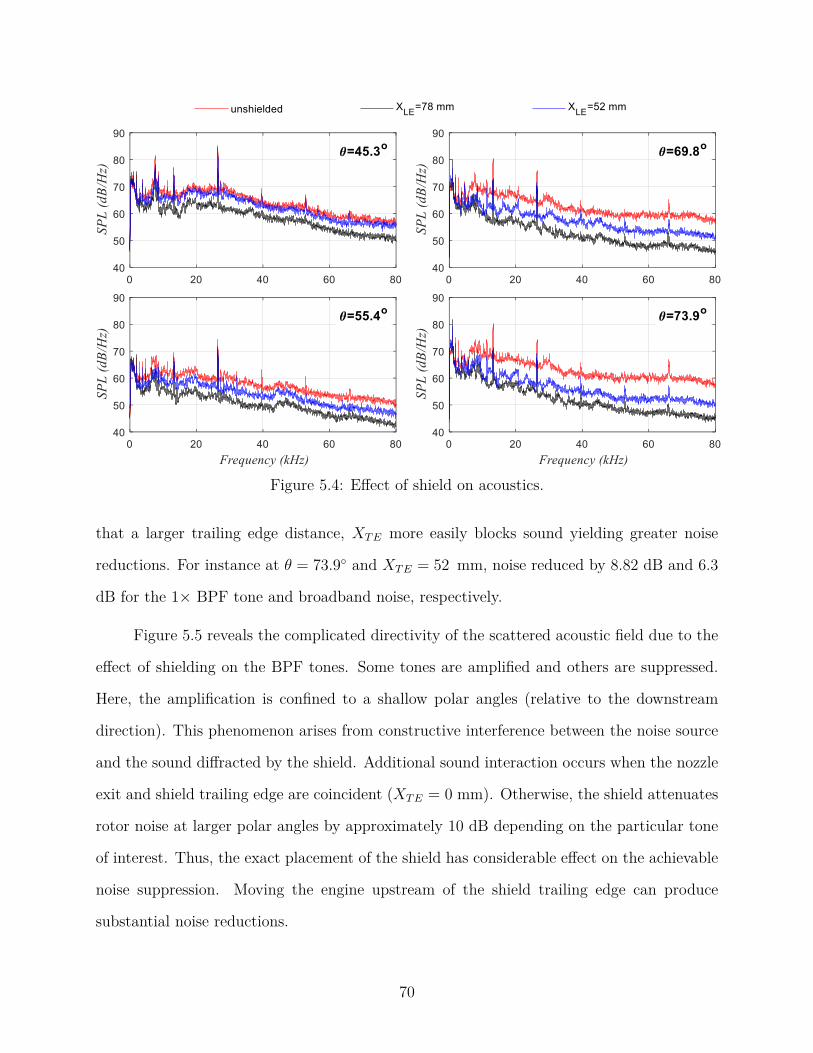
Figure 5.4: Effect of shield on acoustics.
that a larger trailing edge distance, XTE more easily blocks sound yielding greater noise
reductions. For instance at θ = 73.9 and XTE = 52 mm, noise reduced by 8.82 dB and 6.3
dB for the 1× BPF tone and broadband noise, respectively.
Figure 5.5 reveals the complicated directivity of the scattered acoustic field due to the
effect of shielding on the BPF tones. Some tones are amplified and others are suppressed.
Here, the amplification is confined to a shallow polar angles (relative to the downstream
direction). This phenomenon arises from constructive interference between the noise source
and the sound diffracted by the shield. Additional sound interaction occurs when the nozzle
exit and shield trailing edge are coincident (XTE = 0 mm). Otherwise, the shield attenuates
rotor noise at larger polar angles by approximately 10 dB depending on the particular tone
of interest. Thus, the exact placement of the shield has considerable effect on the achievable
noise suppression. Moving the engine upstream of the shield trailing edge can produce
substantial noise reductions.
70
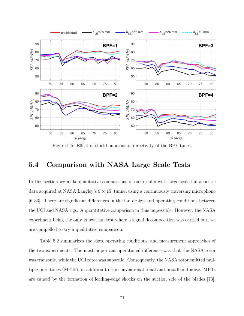
Figure 5.5: Effect of shield on acoustic directivity of the BPF tones.
5.4 Comparison with NASA Large Scale Tests
In this section we make qualitative comparisons of our results with large-scale fan acoustic
data acquired at NASA Langley’s 9’× 15’ tunnel using a continuously traversing microphone
[6, 33]. There are significant differences in the fan design and operating conditions between
the UCI and NASA rigs. A quantitative comparison in thus impossible. However, the NASA
experiment being the only known fan test where a signal decomposition was carried out, we
are compelled to try a qualitative comparison.
Table 5.2 summarizes the sizes, operating conditions, and measurement approaches of
the two experiments. The most important operational difference was that the NASA rotor
was transonic, while the UCI rotor was subsonic. Consequently, the NASA rotor emitted mul-
tiple pure tones (MPTs), in addition to the conventional tonal and broadband noise. MPTs
are caused by the formation of leading-edge shocks on the suction side of the blades [73].
71
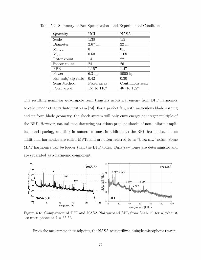
Table 5.2: Summary of Fan Specifications and Experimental Conditions
Quantity UCI NASAScale 1:38 1:5Diameter 2.67 in 22 inMtunnel 0 0.1Mtip 0.60 1.08Rotor count 14 22Stator count 24 26FPR 1.157 1.47Power 6.3 hp 5000 hpFan hub/ tip ratio 0.42 0.30Scan Method Fixed array Continuous scanPolar angle 15 to 110 46 to 152
The resulting nonlinear quadrupole term transfers acoustical energy from BPF harmonics
to other modes that radiate upstream [74]. For a perfect fan, with meticulous blade spacing
and uniform blade geometry, the shock system will only emit energy at integer multiple of
the BPF. However, natural manufacturing variations produce shocks of non-uniform ampli-
tude and spacing, resulting in numerous tones in addition to the BPF harmonics. These
additional harmonics are called MPTs and are often referred to as “buzz saw" noise. Some
MPT harmonics can be louder than the BPF tones. Buzz saw tones are deterministic and
are separated as a harmonic component.
NASA SDT
Θ=65.5o
UCI
Figure 5.6: Comparison of UCI and NASA Narrowband SPL from Shah [6] for a exhaustarc microphone at θ = 65.5.
From the measurement standpoint, the NASA tests utilized a single microphone travers-
72
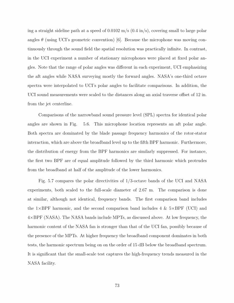
ing a straight sideline path at a speed of 0.0102 m/s (0.4 in/s), covering small to large polar
angles θ (using UCI’s geometric convention) [6]. Because the microphone was moving con-
tinuously through the sound field the spatial resolution was practically infinite. In contrast,
in the UCI experiment a number of stationary microphones were placed at fixed polar an-
gles. Note that the range of polar angles was different in each experiment, UCI emphasizing
the aft angles while NASA surveying mostly the forward angles. NASA’s one-third octave
spectra were interpolated to UCI’s polar angles to facilitate comparisons. In addition, the
UCI sound measurements were scaled to the distances along an axial traverse offset of 12 in.
from the jet centerline.
Comparisons of the narrowband sound pressure level (SPL) spectra for identical polar
angles are shown in Fig. 5.6. This microphone location represents an aft polar angle.
Both spectra are dominated by the blade passage frequency harmonics of the rotor-stator
interaction, which are above the broadband level up to the fifth BPF harmonic. Furthermore,
the distribution of energy from the BPF harmonics are similarly suppressed. For instance,
the first two BPF are of equal amplitude followed by the third harmonic which protrudes
from the broadband at half of the amplitude of the lower harmonics.
Fig. 5.7 compares the polar directivities of 1/3-octave bands of the UCI and NASA
experiments, both scaled to the full-scale diameter of 2.67 m. The comparison is done
at similar, although not identical, frequency bands. The first comparison band includes
the 1×BPF harmonic, and the second comparison band includes 4 & 5×BPF (UCI) and
4×BPF (NASA). The NASA bands include MPTs, as discussed above. At low frequency, the
harmonic content of the NASA fan is stronger than that of the UCI fan, possibly because of
the presence of the MPTs. At higher frequency the broadband component dominates in both
tests, the harmonic spectrum being on on the order of 15 dB below the broadband spectrum.
It is significant that the small-scale test captures the high-frequency trends measured in the
NASA facility.
73
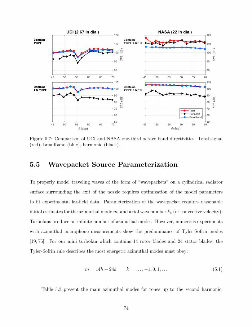
Figure 5.7: Comparison of UCI and NASA one-third octave band directivities. Total signal(red), broadband (blue), harmonic (black).
5.5 Wavepacket Source Parameterization
To properly model traveling waves of the form of “wavepackets” on a cylindrical radiator
surface surrounding the exit of the nozzle requires optimization of the model parameters
to fit experimental far-field data. Parameterization of the wavepacket requires reasonable
initial estimates for the azimuthal modem, and axial wavenumber kz (or convective velocity).
Turbofans produce an infinite number of azimuthal modes. However, numerous experiments
with azimuthal microphone measurements show the predominance of Tyler-Sofrin modes
[19, 75]. For our mini turbofan which contains 14 rotor blades and 24 stator blades, the
Tyler-Sofrin rule describes the most energetic azimuthal modes must obey:
m = 14h+ 24k k = . . . ,−1, 0, 1, . . . (5.1)
Table 5.3 present the main azimuthal modes for tones up to the second harmonic.
74
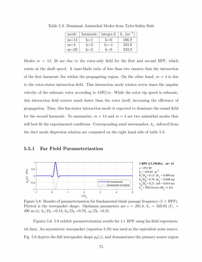
Table 5.3: Dominant Azimuthal Modes from Tyler-Sofrin Rule
mode harmonic integer,k kz (m−1)m=14 h=1 k=0 166.9m=4 h=2 k=-1 334.8m=28 h=2 k=0 333.9
Modes m = 14, 28 are due to the rotor-only field for the first and second BPF, which
rotate at the shaft speed. A vane-blade ratio of less than two ensures that the interaction
of the first harmonic lies within the propagating region. On the other hand, m = 4 is due
to the rotor-stator interaction field. This interaction mode rotates seven times the angular
velocity of the subsonic rotor according to hBΩ/m. While the rotor tip speed is subsonic,
this interaction field rotates much faster than the rotor itself, increasing the efficiency of
propagation. Thus, this fan-stator interaction mode is expected to dominate the sound field
for the second harmonic. To summarize, m = 14 and m = 4 are two azimuthal modes that
will best fit the experimental conditions. Corresponding axial wavenumber, kz, inferred from
the duct mode dispersion relation are computed on the right hand side of table 5.3.
5.5.1 Far Field Parameterization
Figure 5.8: Results of parameterization for fundamental blade passage frequency (1 × BPF).Plotted is the wavepacket shape. Optimum parameters are ε = 291.8, kz = 169.05 (Uc =490 m/s), b1/D0 =0.13, b2/D0 =0.70, z0/D0 =0.21.
Figures 5.8- 5.9 exhibit parameterization results for 1× BPF using far-field experimen-
tal data. An asymmetric wavepacket (equation 3.19) was used as the equivalent noise source.
Fig 5.8 depicts the full wavepacket shape p0(z), and demonstrates the primary source region
75
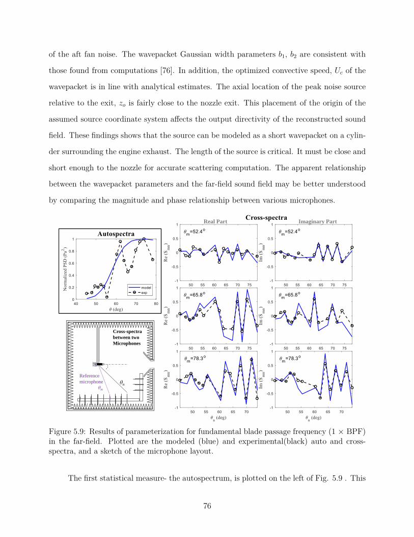
of the aft fan noise. The wavepacket Gaussian width parameters b1, b2 are consistent with
those found from computations [76]. In addition, the optimized convective speed, Uc of the
wavepacket is in line with analytical estimates. The axial location of the peak noise source
relative to the exit, zo is fairly close to the nozzle exit. This placement of the origin of the
assumed source coordinate system affects the output directivity of the reconstructed sound
field. These findings shows that the source can be modeled as a short wavepacket on a cylin-
der surrounding the engine exhaust. The length of the source is critical. It must be close and
short enough to the nozzle for accurate scattering computation. The apparent relationship
between the wavepacket parameters and the far-field sound field may be better understood
by comparing the magnitude and phase relationship between various microphones.
θn
Reference
microphone
θm
Cross-spectra
between two
Microphones
Real Part Imaginary Part
Figure 5.9: Results of parameterization for fundamental blade passage frequency (1 × BPF)in the far-field. Plotted are the modeled (blue) and experimental(black) auto and cross-spectra, and a sketch of the microphone layout.
The first statistical measure- the autospectrum, is plotted on the left of Fig. 5.9 . This
76
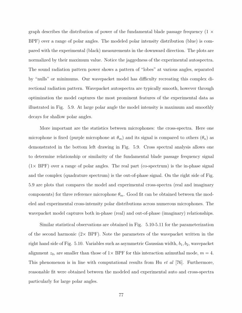
graph describes the distribution of power of the fundamental blade passage frequency (1 ×
BPF) over a range of polar angles. The modeled polar intensity distribution (blue) is com-
pared with the experimental (black) measurements in the downward direction. The plots are
normalized by their maximum value. Notice the jaggedness of the experimental autospectra.
The sound radiation pattern power shows a pattern of “lobes” at various angles, separated
by “nulls” or minimums. Our wavepacket model has difficulty recreating this complex di-
rectional radiation pattern. Wavepacket autospectra are typically smooth, however through
optimization the model captures the most prominent features of the experimental data as
illustrated in Fig. 5.9. At large polar angle the model intensity is maximum and smoothly
decays for shallow polar angles.
More important are the statistics between microphones: the cross-spectra. Here one
microphone is fixed (purple microphone at θm) and its signal is compared to others (θn) as
demonstrated in the bottom left drawing in Fig. 5.9. Cross spectral analysis allows one
to determine relationship or similarity of the fundamental blade passage frequency signal
(1× BPF) over a range of polar angles. The real part (co-spectrum) is the in-phase signal
and the complex (quadrature spectrum) is the out-of-phase signal. On the right side of Fig.
5.9 are plots that compares the model and experimental cross-spectra (real and imaginary
components) for three reference microphone θm. Good fit can be obtained between the mod-
eled and experimental cross-intensity polar distributions across numerous microphones. The
wavepacket model captures both in-phase (real) and out-of-phase (imaginary) relationships.
Similar statistical observations are obtained in Fig. 5.10-5.11 for the parameterization
of the second harmonic (2× BPF). Note the parameters of the wavepacket written in the
right hand side of Fig. 5.10. Variables such as asymmetric Gaussian width, b1, b2, wavepacket
alignment z0, are smaller than those of 1× BPF for this interaction azimuthal mode, m = 4.
This phenomenon is in line with computational results from Hu et al [76]. Furthermore,
reasonable fit were obtained between the modeled and experimental auto and cross-spectra
particularly for large polar angles.
77
Figure 5.10: Results of parameterization for 2nd harmonic (2 × BPF). Plotted is thewavepacket shape. Optimum parameters are ε = 292.0, kz = 312.57 (Uc = 530.68 m/s),b1/D0 =0.10, b2/D0 =0.50, z0/D0 =0.12.
Real Part Imaginary Part
θn
Reference
microphone
θm
Cross-spectra
between two
Microphones
Figure 5.11: Results of parameterization for fundamental blade passage frequency (2 ×BPF) in the far-field. Plotted are the modeled (blue) and experimental (black) auto andcross-spectra, and a sketch of the microphone layout.
5.5.2 Near Field Statistics and Parameterization
It is important to realize that far-field phased array measurements detect only the radiating
part of the noise source. Acquiring pressure signals just outside the mixing layer by an near-
78
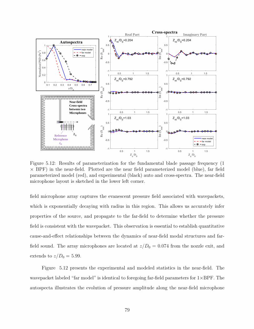
Real Part Imaginary Part
Reference
Microphone
zm
Near-field
Cross-spectra
between two
Microphones
zn
Figure 5.12: Results of parameterization for the fundamental blade passage frequency (1× BPF) in the near-field. Plotted are the near field parameterized model (blue), far fieldparameterized model (red), and experimental (black) auto and cross-spectra. The near-fieldmicrophone layout is sketched in the lower left corner.
field microphone array captures the evanescent pressure field associated with wavepackets,
which is exponentially decaying with radius in this region. This allows us accurately infer
properties of the source, and propagate to the far-field to determine whether the pressure
field is consistent with the wavepacket. This observation is essential to establish quantitative
cause-and-effect relationships between the dynamics of near-field modal structures and far-
field sound. The array microphones are located at z/D0 = 0.074 from the nozzle exit, and
extends to z/D0 = 5.99.
Figure 5.12 presents the experimental and modeled statistics in the near-field. The
wavepacket labeled “far model” is identical to foregoing far-field parameters for 1×BPF. The
autospecta illustrates the evolution of pressure amplitude along the near-field microphone
79
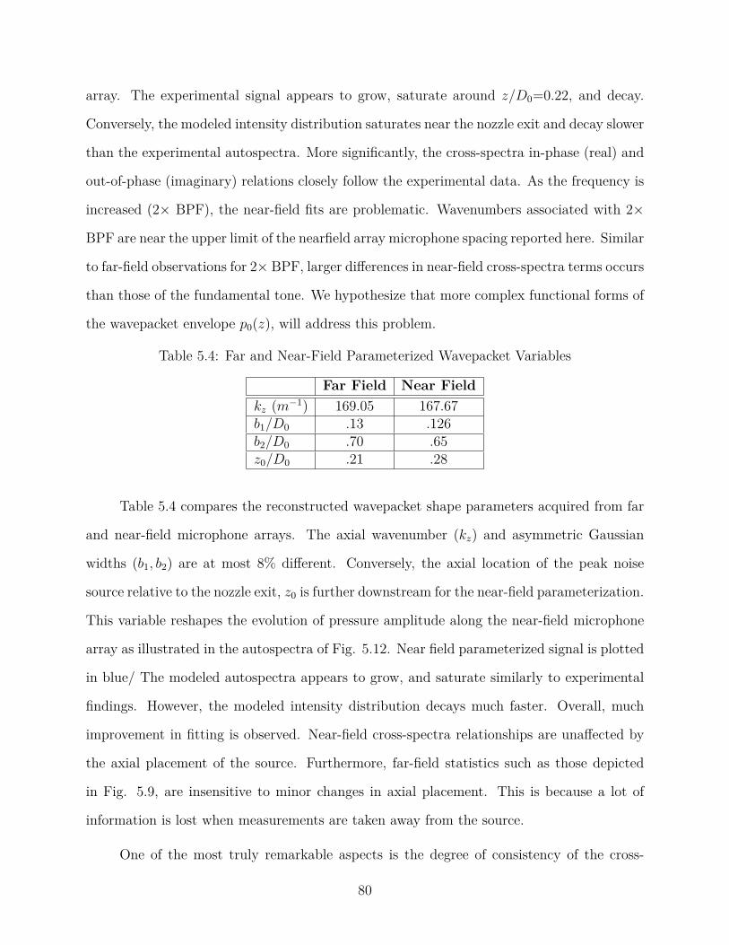
array. The experimental signal appears to grow, saturate around z/D0=0.22, and decay.
Conversely, the modeled intensity distribution saturates near the nozzle exit and decay slower
than the experimental autospectra. More significantly, the cross-spectra in-phase (real) and
out-of-phase (imaginary) relations closely follow the experimental data. As the frequency is
increased (2× BPF), the near-field fits are problematic. Wavenumbers associated with 2×
BPF are near the upper limit of the nearfield array microphone spacing reported here. Similar
to far-field observations for 2× BPF, larger differences in near-field cross-spectra terms occurs
than those of the fundamental tone. We hypothesize that more complex functional forms of
the wavepacket envelope p0(z), will address this problem.
Table 5.4: Far and Near-Field Parameterized Wavepacket Variables
Far Field Near Fieldkz (m−1) 169.05 167.67b1/D0 .13 .126b2/D0 .70 .65z0/D0 .21 .28
Table 5.4 compares the reconstructed wavepacket shape parameters acquired from far
and near-field microphone arrays. The axial wavenumber (kz) and asymmetric Gaussian
widths (b1, b2) are at most 8% different. Conversely, the axial location of the peak noise
source relative to the nozzle exit, z0 is further downstream for the near-field parameterization.
This variable reshapes the evolution of pressure amplitude along the near-field microphone
array as illustrated in the autospectra of Fig. 5.12. Near field parameterized signal is plotted
in blue/ The modeled autospectra appears to grow, and saturate similarly to experimental
findings. However, the modeled intensity distribution decays much faster. Overall, much
improvement in fitting is observed. Near-field cross-spectra relationships are unaffected by
the axial placement of the source. Furthermore, far-field statistics such as those depicted
in Fig. 5.9, are insensitive to minor changes in axial placement. This is because a lot of
information is lost when measurements are taken away from the source.
One of the most truly remarkable aspects is the degree of consistency of the cross-
80
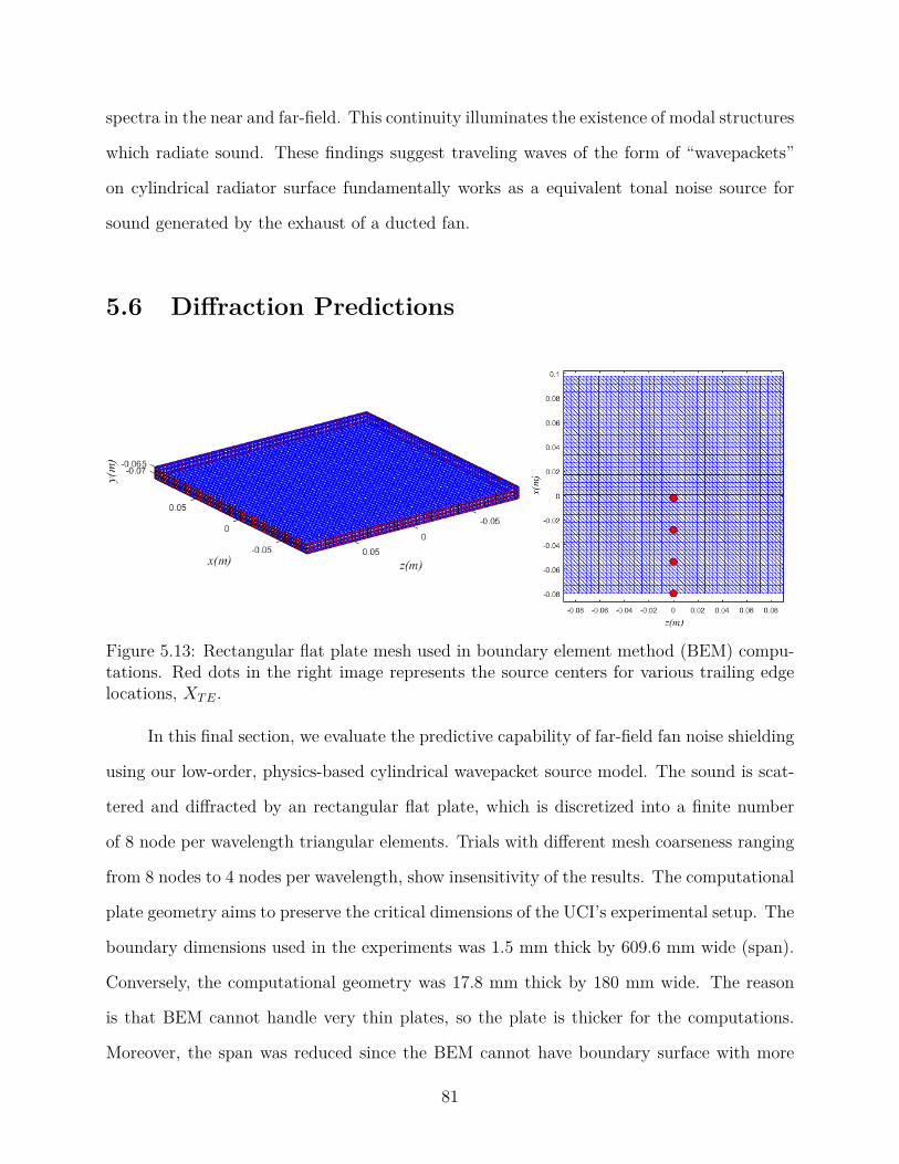
spectra in the near and far-field. This continuity illuminates the existence of modal structures
which radiate sound. These findings suggest traveling waves of the form of “wavepackets”
on cylindrical radiator surface fundamentally works as a equivalent tonal noise source for
sound generated by the exhaust of a ducted fan.
5.6 Diffraction Predictions
Figure 5.13: Rectangular flat plate mesh used in boundary element method (BEM) compu-tations. Red dots in the right image represents the source centers for various trailing edgelocations, XTE.
In this final section, we evaluate the predictive capability of far-field fan noise shielding
using our low-order, physics-based cylindrical wavepacket source model. The sound is scat-
tered and diffracted by an rectangular flat plate, which is discretized into a finite number
of 8 node per wavelength triangular elements. Trials with different mesh coarseness ranging
from 8 nodes to 4 nodes per wavelength, show insensitivity of the results. The computational
plate geometry aims to preserve the critical dimensions of the UCI’s experimental setup. The
boundary dimensions used in the experiments was 1.5 mm thick by 609.6 mm wide (span).
Conversely, the computational geometry was 17.8 mm thick by 180 mm wide. The reason
is that BEM cannot handle very thin plates, so the plate is thicker for the computations.
Moreover, the span was reduced since the BEM cannot have boundary surface with more
81
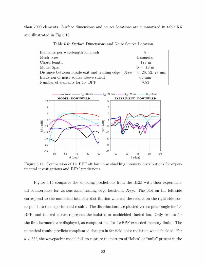
than 7000 elements. Surface dimensions and source locations are summarized in table 5.5
and illustrated in Fig 5.13.
Table 5.5: Surface Dimensions and Noise Source Location
Elements per wavelength for mesh 8Mesh type triangularChord length .178 mModel Span S = .18 mDistance between nozzle exit and trailing edge XTE = 0, 26, 52, 78 mmElevation of noise source above shield 65 mmNumber of elements for 1× BPF 7083
Figure 5.14: Comparison of 1× BPF aft fan noise shielding intensity distributions for exper-imental investigations and BEM predictions.
Figure 5.14 compares the shielding predictions from the BEM with their experimen-
tal counterparts for various axial trailing edge locations, XTE. The plot on the left side
correspond to the numerical intensity distribution whereas the results on the right side cor-
responds to the experimental results. The distributions are plotted versus polar angle for 1×
BPF, and the red curves represent the isolated or unshielded ducted fan. Only results for
the first harmonic are displayed, as computations for 2×BPF exceeded memory limits. The
numerical results predicts complicated changes in far-field noise radiation when shielded. For
θ < 55, the wavepacket model fails to capture the pattern of “lobes” or “nulls” present in the
82
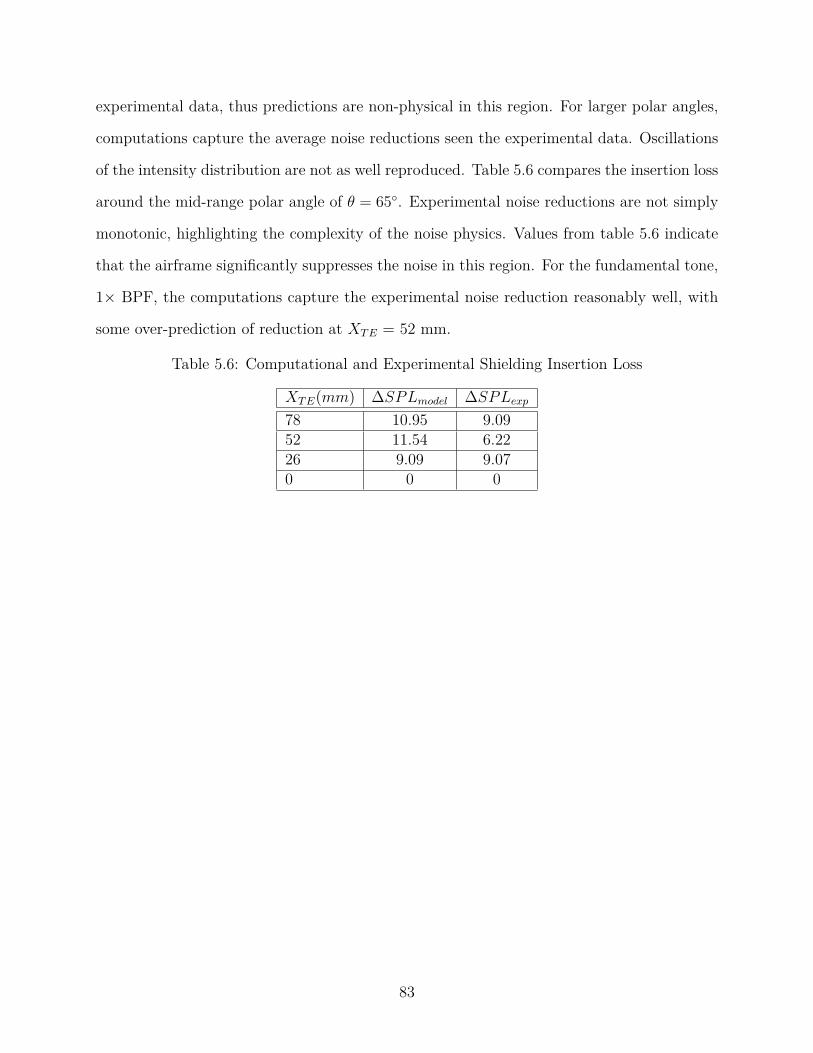
experimental data, thus predictions are non-physical in this region. For larger polar angles,
computations capture the average noise reductions seen the experimental data. Oscillations
of the intensity distribution are not as well reproduced. Table 5.6 compares the insertion loss
around the mid-range polar angle of θ = 65. Experimental noise reductions are not simply
monotonic, highlighting the complexity of the noise physics. Values from table 5.6 indicate
that the airframe significantly suppresses the noise in this region. For the fundamental tone,
1× BPF, the computations capture the experimental noise reduction reasonably well, with
some over-prediction of reduction at XTE = 52 mm.
Table 5.6: Computational and Experimental Shielding Insertion Loss
XTE(mm) ∆SPLmodel ∆SPLexp78 10.95 9.0952 11.54 6.2226 9.09 9.070 0 0
83

6
Cha
pter
Conclusion and Future Work
A large number of experiments in uninstalled and installed configurations have validated
the capability of the small-scale rig to reproduce the fan noise emitted by the turbofan
engine and have demonstrated the large potential to reduce noise through shielding by the
airframe. Complementing our earlier studies of the isolated and installed small-scale ducted
fan [29], this work demonstrates that important aspects of fan noise can be studied at
low cost in university-scale facilities, leveraging advances in additive manufacturing and
brushless motor technology. The rapid-prototyped ducted fan featured a 14-bladed rotor
and 24 stators, and operated at fan pressure ratio of 1.157 and rotor tip Mach number of
0.61. Its operation was representative of future geared turbofan engines with very large
bypass ratio.
This project demonstrated the application of Vold-Kalman filtering of aeroacoustic
measurements from a small scale ducted fan, for the purpose of rigorously determining the
harmonic and broadband components of noise. Knowledge of the tonal and broadband noise
content is essential for characterizing the fan noise source and predicting propulsion-airframe
integration effects. A second-generation Vold-Kalman filter was employed to separate the
time-domain contributions of harmonic and broadband contents. This filter is advantageous
to frequency domain methods since it can easily localize information with high resolution
needed to correct for the non-stationary behavior in real world experiments.
84
Fan exhaust discrete tone noise was modeled as a cylindrical wavepacket with azimuthal
modes inferred from the Tyler-Sofrin theory and shape parameters determined through least-
squares matching of the experimental Vold-Kalman filtered tonal cross-spectral density in
the far field. A asymmetric wavepacket was used as the equivalent noise source. This
framework provides, a deterministic model that capture the salient physics of the source and
that allow understanding and enable predictions of the radiated sound and its scattering
around objects without inordinate computational resources. Parameterization shows that
the amplitude modulated traveling wave on a control surface (Kirchhoff) surrounding the
exit of the nozzle can be modeled as short cylindrical disturbances. The length of the source
is critical since it must be close and short enough to the nozzle for accurate scattering
computation. Our wavepacket model captures the most prominent far-field and near-field
experimental magnitude and phase relationship across numerous microphone (i.e. cross-
spectra distribution). One of the most truly remarkable aspects is the degree of consistency
of the cross-spectra in the near and far-field. This continuity illuminates the existence
of modal structures which radiate sound. These promising results indicate that the noise
radiated by modal structures in the form of traveling waves or “wavepackets” fundamentally
works as a equivalent tonal noise source for sound generated by the exhaust of a ducted fan.
Installation of a rectangular flat plate representing the airframe enables experimental
studies of the diffraction of the sound emitted by the ducted fan. Addition of the rectangular
plate shield created complex trends in the tonal content and demonstrated the large potential
to reduce noise through shielding by the airframe. Tones below the shielding surface were
well attenuated, while tones emitted in the aft direction were poorly shielded. Numerical
shielding prediction using Boundary element method (BEM) exhibit complicated changes in
far-field noise radiation. For θ < 55 the wavepacket model fails to capture the pattern of
“lobes” or “nulls” present in the experimental data, thus predictions are non-physical in this
region. For larger polar angles, computations capture the average noise reductions as seen
in experimental data. Oscillations of the intensity distribution are not as well reproduced.
85

This new framework provide more general methods for the effects related to propulsion
airframe aeroacoustic interaction, and allows for low-noise optimization of the BWB aircraft
with an ultra high bypass propulsor. In addition, such improvements strengthen insight and
understanding into controlling noise physics.
6.1 Recommendations For Future Work
The semi-empirical fan noise source model was calibrated to takeoff conditions. As the fan tip
speed varies across the operating regime of the engine, the properties of the wavepacket shape
changes. Future revisions to this framework includes the parameterization of experimental
data simulating the certification points of approach and cutback (61.7% and 87.5% of design
conditions, respectively). Furthermore, the mechanisms that generate aft-radiated noise are
similar to those that generate the forward-radiated noise. Therefore, the wavepacket can be
reframed to model inlet radiated noise in future explorations.
To expand this model to cover a wide range of fan diameters, mass flow rate, and
fan pressure ratio, the current “state of the art” in empirical predictions (ANOPP module
HDNFAN) utilizes the Heidmann normalization as part of its underlying framework [77].
This amounts to simple sound pressure level corrections based on the fan temperature rise
and mass flow rate. One limitation to more complex corrections concerns the experimental
data used to formulate the model. In other words, acoustical experiments investigating
numerous engine operating conditions and configurations are prohibitively expensive and
laborious. CFD provides a relatively low cost and useful way to assess the effect of geometry,
shape, and flow conditions on the noise propagation and directivity. These computational
solutions can inform the prescription of the noise source on the radiator surface [17].
Several topics were not thoroughly examined in the present work due to complications.
Significant effort was entailed in the design and construction of a small-scaled ducted fan rig
that includes all the relevant components of the turbofan engine and simulates accurately
86

the sound emission generated by the fan of such engines. The nacelle (including the stators)
were fabricated during a previous investigation using simple thermodynamic relations and
specified camber (metal angles). Redesign of the fan for improved reliability using aluminum
metal casting and more advanced turbomachinery design codes enhanced the compression
capability. As a result, the originally designed stator pitch and metal angles may not recover
the induced tangential velocity as proficiently, lowering the thrust performance of the engine.
However, since this fan was meant to be representative of current technology, this compromise
was deemed to be acceptable for this test. Future experiments involving low-noise stator
designs such as stator sweep or lean dictates the re-optimization of this baseline radial stator
set.
Another obstacle was the 7000 element limit for regular BEM diffractions simulations.
This constraint entails reducing the computational domain (i.e. wing span) and low spatial
grid resolution (4 nodes per wavelength) to get inside the limit. Trials with different mesh
coarseness show insensitivity of the results with the finest mesh containing 8 nodes per wave-
length. In addition, minor changes in intensity distribution emerged with increasing wing
span. However, computations for 2×BPF failed since it exceeded element limits. FastBEM
can handle much larger matrices, possible up to 10,000 elements and is sold commercially
through CAE Research lab. Extensive comparisons between conventional and fastBEM will
provide confidence in predictions. Additionally, this tool can provide insight into realistic
shield geometry such as the BWB. In addition, acoustical impacts such as the placement
of the engines, geometry of elevon, and positioning and shape of the vertical fins can be
numerically predicted.
Future enhancement to this approach of simulating fan noise is to increase power. An
power boost permits operating at higher fan pressure ratio such as those found at NASA
Glenn which operate at FPR=1.46. Power can increase from 5 kW (FPR=1.15) to 14 kW
(FPR=1.29) or 22 kW (FPR=1.46) depending on components. This is accomplished two
ways: increasing the voltage or capacity of the battery. The lithium-polymer pack and the
87
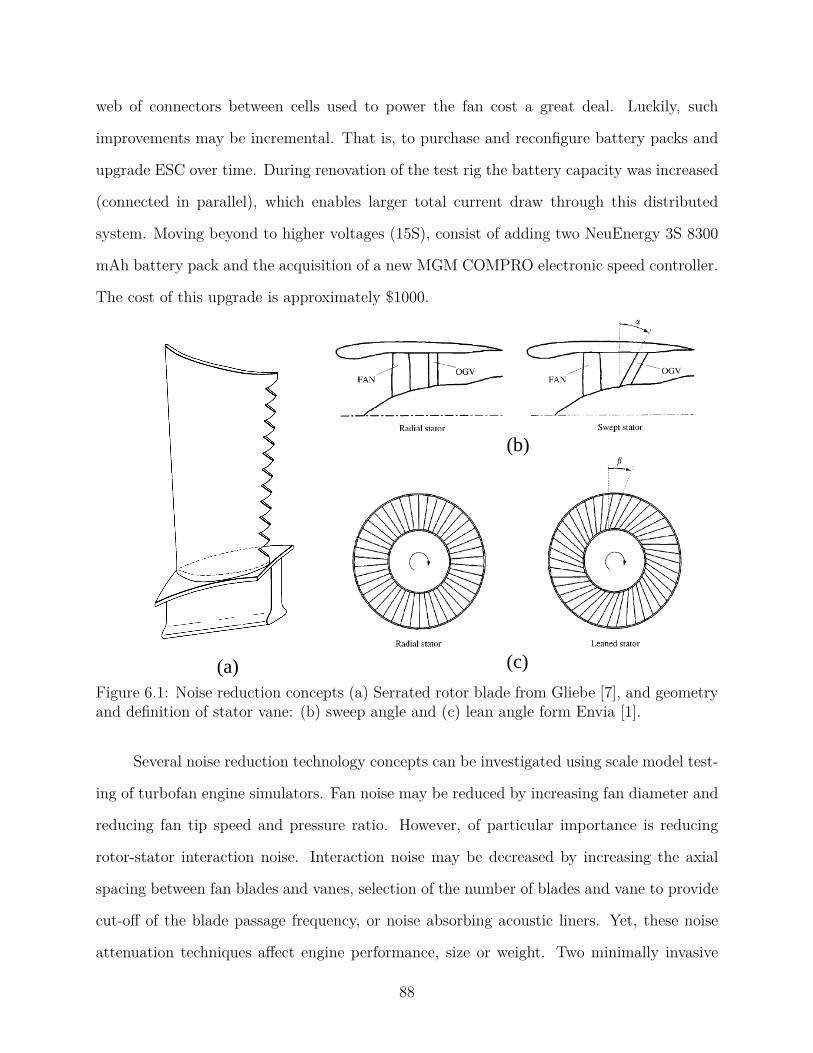
web of connectors between cells used to power the fan cost a great deal. Luckily, such
improvements may be incremental. That is, to purchase and reconfigure battery packs and
upgrade ESC over time. During renovation of the test rig the battery capacity was increased
(connected in parallel), which enables larger total current draw through this distributed
system. Moving beyond to higher voltages (15S), consist of adding two NeuEnergy 3S 8300
mAh battery pack and the acquisition of a new MGM COMPRO electronic speed controller.
The cost of this upgrade is approximately $1000.
(a)
(b)
(c)
Figure 6.1: Noise reduction concepts (a) Serrated rotor blade from Gliebe [7], and geometryand definition of stator vane: (b) sweep angle and (c) lean angle form Envia [1].
Several noise reduction technology concepts can be investigated using scale model test-
ing of turbofan engine simulators. Fan noise may be reduced by increasing fan diameter and
reducing fan tip speed and pressure ratio. However, of particular importance is reducing
rotor-stator interaction noise. Interaction noise may be decreased by increasing the axial
spacing between fan blades and vanes, selection of the number of blades and vane to provide
cut-off of the blade passage frequency, or noise absorbing acoustic liners. Yet, these noise
attenuation techniques affect engine performance, size or weight. Two minimally invasive
88
concepts are proposed . First are serrated fan trailing edges blades. Serrations like chevrons
aim to mix the downstream moving viscous waves due to the rotor velocity deficit before
interacting with the stator leading edge. This reduces the instationary stator blade forces
that generates noise [78]. Another way to target the noise generated by the periodic im-
pingement of fan wakes on the vanes are low-noise stator design. Sweeping and leaning the
outlet guide vane have shown noise reductions of 5 dB for the inlet quadrant and 10 dB for
the exhaust quadrant for all angles [1]. Here, tone noise is reduced by introducing a phase
variation along the span of the vane, from the hub to the tip. When the rotor wake moves
downstream it does not strike the stator leading edge all at once reducing the impact of
rotor-stator interaction. On the other hand, phase variation by asymmetric stator spacing
appears to have “no practical value” according to Sofrin [79]. This report studied the noise
benefit for stators with small random variations (due to manufacturing imperfections) from
precisely equal spacing in the circumferential direction. Acoustic test suggested asymmetry
spreads the acoustic energy over a larger number of modes and was a source of extraneous
sound. Studies on optimal non-random uneven stator spacing using psychoacoustic metrics
are nonexistent and may be a topic of future exploration.
89
Bibliography
[1] E. Envia, A. Wilson, and D. Huff, “Fan noise: A challenge to caa,” International Jourof Comp Fluid Dyn, vol. 18, pp. 471–480, 2004.
[2] S. Rienstra, “Acoustic radiation from a semi-infinite annular duct in a uniform subsonicmean flow,” Journal of Fluid Mechs, vol. 94, pp. 267–175, 1984.
[3] X. Huang and X. Chen, “Efficient computation of spinning modal radiation through anengine bypass duct,” AIAA Journal, vol. 46, pp. 1413–1423, June 2008.
[4] S. Redonnet and Y. Druon, “Computational aeroacoustics of aft fan noises characteriz-ing a realistic coaxial engine,” AIAA Journal, vol. 50, pp. 1029–1048, 2012.
[5] G. Reboul and C. Polacsek, “Toward numerical simulation of fan broadband noise aftradiation from aeroengines,” AIAA Journal, vol. 48, pp. 2038–2048, 2010.
[6] P. Shah, H. Vold, D. Hensley, E. Envia, and D. Stephens, “A high-resolution, continuous-scan acoustic measurement method for turbofan engine applications,” ASME PaperGT2014-27108, June 2014.
[7] P. Gliebe, “Serrated fan blade,” US Patent 4,741,207, May 2004.
[8] B. Magliozzi, D. Hanson, and R. Amiet, “Propeller and profan noise,” Tech. Rep. N92-10598 01-71, NASA Langley Research Center, Hampton, VA, July 1991.
[9] M. J. Lighthill, “On sound generated aerodynamically: I. general theory,” Proceedingsof the Royal Society of London, vol. 211, pp. 564–587, 1952.
[10] J. Groeneweg and E. Rice, “Aircraft turbofan noise,” Trasactions of the ASME, vol. 109,pp. 130–140, 1987.
[11] R. Liebeck, “Design of the blended wing body subsonic transport,” Journal of Aircraft,vol. 41, no. 1, pp. 10–25, 2004.
[12] S. Mayoral and D. Papamoschou, “Effects of source redistribution on jet noise shielding,”AIAA 2010-0652, Jan. 2010.
[13] R. Thomas and C. Burley, “Hybrid wing body aircraft system noise assesment withpropulsion airframe aeroacoustic experiments,” AIAA 2010-3913, June 2010.
90
[14] J. Berton, “Empennage noise shielding benefits for an open rotor transport,” AIAA2011-2764, June 2011.
[15] A. Truong and D. Papamoschou, “Aeroacoustic testing of open rotors at very smallscale,” AIAA 2013-0217, jan 2013.
[16] D. Papamoschou, “Prediction of jet noise shielding,” AIAA 2010-0653, Jan. 2010.
[17] D. Papamoschou, J. Xiong, and F. Liu, “Towards a low-cost wavepacket model of thejet noise source,” AIAA 2015-1006, Jan. 2015.
[18] P. Jordan and T. Colonius, “Wave packets and turbulent jet noise,” Annual Review ofFluid Mechanics, vol. 45, pp. 173–195, 2013.
[19] T. Sofrin, “Some modal-frequency spectra of fan noise,” AIAA 1981-1990, October 1981.
[20] J. Tyler and T. Sofrin, “Axial flow compressor noise studies,” Transactions of the SAE,vol. 70, pp. 309–332, 1962.
[21] A. Topol, C. Ingram, M. Larkin, C. Roche, and R. Thulin, “Advanced subsonic tech-nonolgy (ast) 22-inch low noise research fan rig preliminary design of adp-type fan 3,”Tech. Rep. NASA/CR-2004-212718, NASA Langley Research Center, Hampton, VA,Feb 2004.
[22] C. Hughes, R. Jeracki, R. Woodward, and C. Miller, “Fan noise source diagnoistictest-rotor alone aerodynamics performance results,” NASA/TM-2005-211681 (AIAA-2002-2426), Apr. 2005.
[23] L. Heidelberg, “Fan noise source diagnostic test - tone model structure results,”NASA/TM-2002-211594 (AIAA-2002-2428), Apr. 2002.
[24] B. Morin, “Broadband fan noise prediction system for turbofan engines, volume 1: Setupbfans user’s manual and developer’s guide,” Tech. Rep. CR-2010-216898, NASA, Nov2010.
[25] B. Morin, “Broadband fan noise prediction system for turbofan engines, volume 3:Validation and test cases,” Tech. Rep. CR-2010-216898, NASA, Nov 2010.
[26] C. Hughes, R. Jeracki, R. Woodward, and C. Miller, “Aerodynamic performance of scale-model turbofan outlet guide vanes designed for low noise,” NASA/TM-2001-211352(AIAA-2002-0374), Dec. 2001.
[27] R. Woodward, “Comparison of far-field noise for three significantly different modelturbofans,” AIAA Paper 2008-0049, Jan 2008.
[28] R. Woodward, D. Elliott, C. Higher, and J. Berton, “Benefits of swept-and-leanedstators for fan noise reduction,” AIAA Journal, vol. 38, no. 6, 2001.
[29] A. Truong and D. Papamoschou, “Experimental simulation of ducted fan acoustics atvery small scale,” AIAA 2014-0718, jan 2014.
91
[30] A. Parry, M. Kingan, and B. Tester, “Relative importance of open rotor tone andbroadband noise sources,” AIAA 2011-2763, June 2011.
[31] D. Stephens and E. Envia, “Acoustic shielding for a model scale counter-rotation openrotor,” NASA/TM-2012-217227 (AIAA-2011-2940), Jan. 2012.
[32] D. Sree and D. Stephens, “Tone and broadband noise separation from acoustic data ofa scale-model counter-rotating open rotor,” AIAA 2014-2744, June 2014.
[33] D. Stephens and H. Vold, “Order tracking signal processing for open rotor acoustics,”Journal of Sound and Vibration, vol. 333, no. 16, pp. 3818–830, 2014.
[34] M. Smith, Aircraft Noise. Cambridge: Cambridge University Press„ 1st ed., 1989.
[35] C. Ventres, M. Theobald, and W. Mark, “Turbofan noise generation volume 1: Analy-sis,” Tech. Rep. CR-167952, NASA Lewis Research Center, Cleveland, OH, July 1982.
[36] W. Eversman and D. Roy, “Ducted fan acoustic radiation including the effects of mo-nuniform mean flow and acoustic treatment,” AIAA 93-4424, Oct. 1993.
[37] D. Huff, “Fan noise prediction - status and needs,” NASA/TM-1997-206533 (AIAA-1997-177), Jan. 1997.
[38] B. Mugridge, “The measurement of spinning acoustic modes generated in an axial flowfan,” Journal Sound Vib., vol. 10, no. 2, pp. 227–246, 1969.
[39] S. Grace, D. Sondak, W. Eversman, and M. Cannamela, “Hybrid prediction of fan tonalnoise,” AIAA 2008-29921, June 2008.
[40] J. Anderson, Modern Compressible Flow: With Historical Perspective. New York:McGraw-Hill, 3rd ed., 2003.
[41] R. Haberman, Applied partial differential equations. New Kersey: Pearspm Pentice Ha;;,4th ed., 2004.
[42] E. Rice, M. Heidmann, and T. Sofrin, “Modal propagation angles in a cylindrical ductwith flow and there relation to sound radiation,” Jan. 1979.
[43] W. Stack, G. Knip, A. Weisbrich, J. Godston, and E. Bradley, “Technology and benefitsof aircraft counter rotation propellers,” NASA Technical Memorandum, Oct 1982.
[44] S. Rienstra, “A classification of duct modes based on surface waves,” AIAA 2001-2180,2001.
[45] G. Gabard and R. Astley, “Theoretical model for sound radiation from annular jet pipes:far- and near-field solutions,” Journal of Fluid Mechanics, vol. 549, pp. 315–341, Feb.2006.
[46] M. R., “The interaction of sound with a subsonic jet issuing from a semi-infinite cylin-drical pipe,” Journal Fluid Mech., vol. 83, no. 4, pp. 609–640, 1977.
92
[47] P. Sijtsma, “In-duct and far-field mode detection techniques,” AIAA 2007-3439, 2007.
[48] D. Sutliff, “Rotating rake turbofan duct mode measurement system,” NASA/TM-2005-213828, Oct. 2005.
[49] C. Tam and D. Burton, “Sound generation by the instability waves of supersonic flows.part 1. two-dimensional mixing layers,” Journal of Fluid Mechanics, vol. 138, pp. 241–279, 1984.
[50] D. Crighton and P. Huerre, “Shear-layer pressure fluctuations and superdirective acous-tic sources,” Journal of Fluid Mechanics, vol. 220, pp. 355–368, 1990.
[51] E. J. Avital, N. D. Sandham, and K. H. Luo, “Mach wave radiation by mixing layers.part i: Analysis of the sound field,” Theoretical and Computational Fluid Dynamics,vol. 12, pp. 73–90, 1998.
[52] D. Papamoschou, “Wavepacket modeling of the jet noise source,” AIAA 2011-2835, June2011.
[53] P. Morris, “A note on noise generation by large scale turbulent structures in subsonicand supersonic jets,” International Journal of Aeroacoustics, vol. 8, no. 4, pp. 301–316,2009.
[54] P. J. Morris, “Jet noise prediction: Past, present and future,” Canadian Acoustics,vol. 35, no. 3, pp. 16–22, 2007.
[55] D. F. Shanno and K. H. Phua, “Minimization of unconstrained multivariate functions,”ACM Transactions on Mathematical Software, vol. 6, no. 4, pp. 618–622, 1976.
[56] D. Amos, “Algorithm 644: A portable package for bessel functions of a complex argu-ment and nonnegative order,” ACM Transactions on Mathematical Software (TOMS),vol. 12, pp. 265–273, Sept. 1986.
[57] C. Huang and D. Papamoschou, “Numerical study of noise shielding by airframe struc-tures,” May 2008.
[58] M. Dunn and J. Tweed, “The application of a boundary integral equation method tothe prediction of ducted fan engine noise,” NASA 20040086509, 1999.
[59] T. Wu, Boundary Element Acoustics. Boston: WIT Press, 2000.
[60] R. Bullock and I. Johnsen, “Aerodynamic design of axial flow compressor,” NASA-SP-36, Jan. 1965.
[61] H. Vold and J. Leuridan, “High resolution order tracking at extreme slew rates usingkalman tracking filters,” SAE Technical Paper 931288, May 1993.
[62] J. Tuma, “Setting the passband width in the vold-kalman tracking filter,” 12th Inter-national Congress on Sound and Vibration, July 2005.
93
[63] C. Feldbauer and R. Holdrich, “Realization of a vold-kalman tracking filter- a leastsquares problem,” Proceedings of the COST-6 Conference on Digital Audio Effects(DAFX-00), Dec. 2000.
[64] R. Kalman, “A new approach to linear filtering and prediction problems,” Journal ofBasic Engineering, Transactions of ASME, vol. 82, pp. 35–45, 1960.
[65] H. Herlufsen, S. Gade, K. Hansen, and H. Vold, “Characteristics of the vold-kalmanorder tracking filter,” Bruel and Kjaer Technical Review, Apr. 1999.
[66] H. Wold, A Study in the Analysis of Stationary Time Series. PhD thesis, StockhomUniversity, 1938.
[67] N. Huang, M. Wu, W. Qu, S. Long, and S. Shen, “Applications of hilbert-huang trans-form to non-stationary financial time series analysis,” pp. 245–268, May 2009.
[68] M. Cohen, "Analyzing Neural Time Series Data". Cambridge: "The MIT Press".
[69] R. Oweis and E. Abdulhay, “Seizure classification in eeg signals utilizing hilbert-huangtrasnform,” Biomedical Engineering Online, pp. 10–38, May 2011.
[70] M. Feldman, “Hilbert transform in vibration analysis,” Mechanical Systems and SignalProcessing, vol. 25, pp. 735–802, Apr. 2011.
[71] L. Cohen and C. Lee, “Standard deviation of instantaneous frequency,” Acoustic, Speech,and Signal Processing, vol. 4, pp. 2238–2241, 1989.
[72] I. Kovacic and M. Brennan, The Duffing Equation: Nonlinear Oscillators and theirBehavior. New Jersey: John Wiley and Sons, 1st ed., 2011.
[73] A. Goldstein, F. Glaser, and J. Coats, “Acoustic properties of a supersonic fan,”NASA/TN-1973-15025, Jan. 1973.
[74] F. Han, C. Shieh, A. Sharma, and U. Paliath, “Multiple pure tone noise prediction andcomparison with static engine test measurement,” AIAA 2007-3523, May 2007.
[75] A. Maldonado, R. Miserda, and B. Pimenta, “Computational tonal noise prediction forthe advanced noise control fan,” AIAA 2012-2128, 2012.
[76] F. Hu and X. Li, “Time domain wave packet method and suppression of instabilitywaves in aeroacoustic computations,” Journal of the Fluids Eng., June 2014.
[77] M. Heidmann, “Interim prediction method for fan and compressor source noise,”NASA/TM X-71763, 1979.
[78] D. Geiger, “Comparative analysis of serrated trailing edge designs on idealized aircraftengine fan blades for noise reduction,” Master’s thesis, Virginia Polytechnic Institute,Dec. 2004.
94
[79] T. Sofrin and D. Mathews, “Asymmetric stator interaction noise,” Journal of Aircraft,vol. 17, no. 8, pp. 554–560, 1980.
[80] W. Sullivan, J. Turnberg, and J. Violette, “Large-scale advanced prop-fan (lap) bladedesign,” Tech. Rep. CR-174790, NASA, 1984.
95
A
App
endi
x
Aerodynamic Design of a
Sub-Scaled Ducted Fan
Nomenclature
c = Chord: length of stright line connecting LE to TEFPR = Fan pressure ratioi = Incidence angle: difference between the inlet and the leading edge meanline angle.
i=β1 − β∗1 or α1 − α∗1mc = Corrected mass flow rateM = Mach numberP0 = Total pressureT0 = Total temperatureα = Absolute air angle: angle between airstream and the axial directionβ = Relative air angle: angle between airstream and the axial directionα∗ or β∗ = Meanline metal angle: angle between meanline at the blade edge (LE or TE)
and the axial direction, α∗ for stators and β∗ for rotorsγ = Specific heat ratio, γ = 1.4 for airδ = Deviation angle: difference between the exit air angle and the trailing edge
meanline angleδ = β2 − β∗2 or α2 − α∗2ηad = Adiabatic efficiencyηp = Polytropic efficiencyλ = Blockage factorξ = Stagger angle: angle between the chord of a blade and the axial directionρ = Densityσ = Solidity: chord to circumferential distance (spacing) between two blades/ vane.
σ = c/S, S = 2πr/N
96
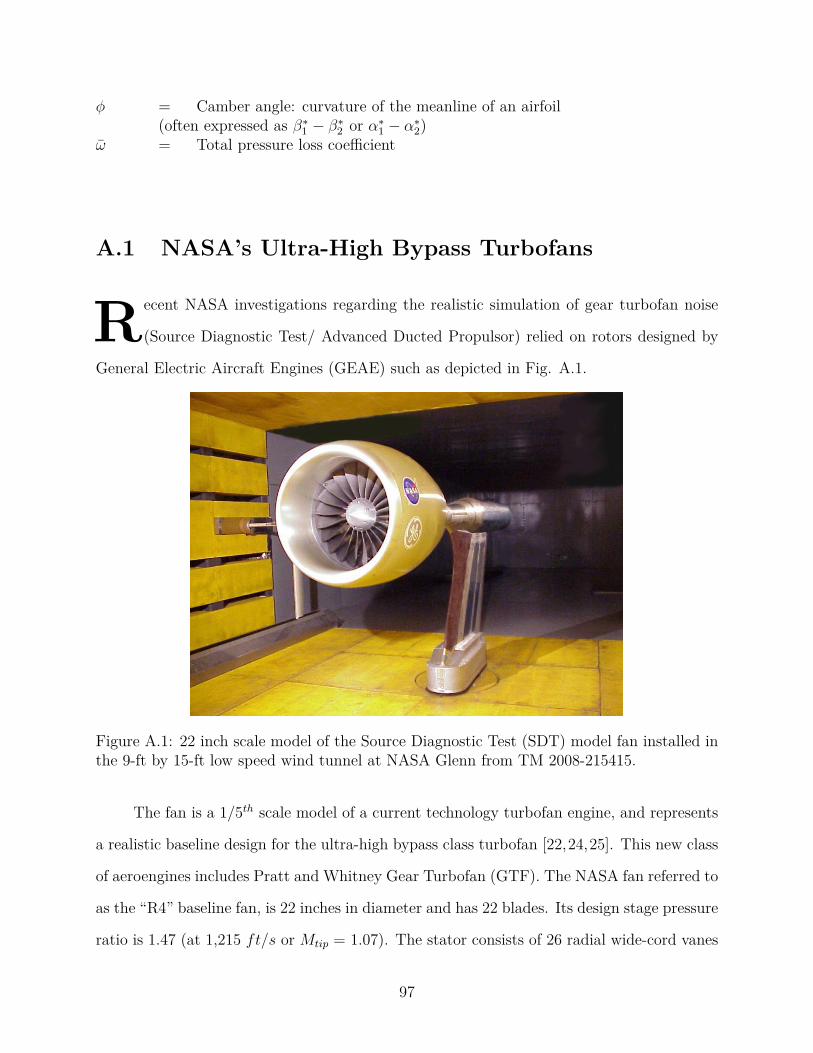
φ = Camber angle: curvature of the meanline of an airfoil(often expressed as β∗1 − β∗2 or α∗1 − α∗2)
ω = Total pressure loss coefficient
A.1 NASA’s Ultra-High Bypass Turbofans
Recent NASA investigations regarding the realistic simulation of gear turbofan noise
(Source Diagnostic Test/ Advanced Ducted Propulsor) relied on rotors designed by
General Electric Aircraft Engines (GEAE) such as depicted in Fig. A.1.
Figure A.1: 22 inch scale model of the Source Diagnostic Test (SDT) model fan installed inthe 9-ft by 15-ft low speed wind tunnel at NASA Glenn from TM 2008-215415.
The fan is a 1/5th scale model of a current technology turbofan engine, and represents
a realistic baseline design for the ultra-high bypass class turbofan [22,24,25]. This new class
of aeroengines includes Pratt and Whitney Gear Turbofan (GTF). The NASA fan referred to
as the “R4” baseline fan, is 22 inches in diameter and has 22 blades. Its design stage pressure
ratio is 1.47 (at 1,215 ft/s or Mtip = 1.07). The stator consists of 26 radial wide-cord vanes
97
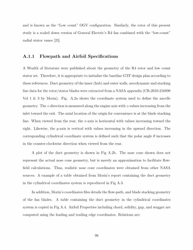
and is known as the “Low count” OGV configuration. Similarly, the rotor of this present
study is a scaled down version of General Electric’s R4 fan combined with the “low-count”
radial stator vanes [23].
A.1.1 Flowpath and Airfoil Specifications
A Wealth of literature were published about the geometry of the R4 rotor and low count
stator set. Therefore, it is appropriate to initialize the baseline GTF design plan according to
these references. Duct geometry of the inner (hub) and outer walls, aerodynamic and stacking
line data for the rotor/stator blades were extracted from a NASA appendix (CR-2010-216898
Vol 1 & 3 by Morin). Fig. A.2a shows the coordinate system used to define the nacelle
geometry. The z-direction is measured along the engine axis with z-values increasing from the
inlet toward the exit. The axial location of the origin for convenience is at the blade stacking
line. When viewed from the rear, the x-axis is horizontal with values increasing toward the
right. Likewise, the y-axis is vertical with values increasing in the upward direction. The
corresponding cylindrical coordinate system is defined such that the polar angle θ increases
in the counter-clockwise direction when viewed from the rear.
A plot of the duct geometry is shown in Fig A.2b. The nose cone shown does not
represent the actual nose cone geometry, but is merely an approximation to facilitate flow-
field calculations. Thus, realistic nose cone coordinates were obtained from other NASA
sources. A example of a table obtained from Morin’s report containing the duct geometry
in the cylindrical coordinates system is reproduced in Fig A.3.
In addition, Morin’s coordinates files details the flow-path, and blade stacking geometry
of the fan blades. A table containing the duct geometry in the cylindrical coordinates
system is copied in Fig A.4. Airfoil Properties including chord, solidity, gap, and stagger are
computed using the leading and trailing edge coordinates. Relations are:
98
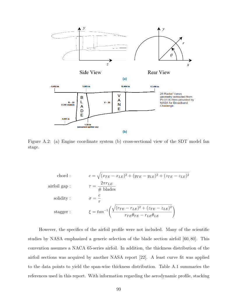
(a)
(b)
Figure A.2: (a) Engine coordinate system (b) cross-sectional view of the SDT model fanstage.
chord : c =√
(xTE − xLE)2 + (yTE − yLE)2 + (zTE − zLE)2
airfoil gap : τ = 2πrLE# blades
solidity : σ = c
τ
stagger : ξ = tan−1(√(rTE − rLE)2 + (zTE − zLE)2
rTEθTE − rLEθLE
)
However, the specifics of the airfoil profile were not included. Many of the scientific
studies by NASA emphasized a generic selection of the blade section airfoil [60, 80]. This
convention assumes a NACA 65-series airfoil. In addition, the thickness distribution of the
airfoil sections was acquired by another NASA report [22]. A least curve fit was applied
to the data points to yield the span-wise thickness distribution. Table A.1 summaries the
references used in this report. With information regarding the aerodynamic profile, stacking
99
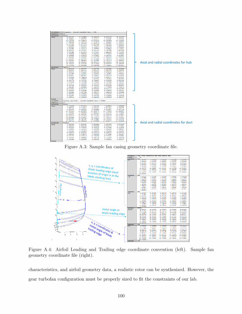
Axial and radial coordinates for hub
Axial and radial coordinates for duct
Figure A.3: Sample fan casing geometry coordinate file.
Figure A.4: Airfoil Leading and Trailing edge coordinate convention (left). Sample fangeometry coordinate file (right).
characteristics, and airfoil geometry data, a realistic rotor can be synthesized. However, the
gear turbofan configuration must be properly sized to fit the constraints of our lab.
100
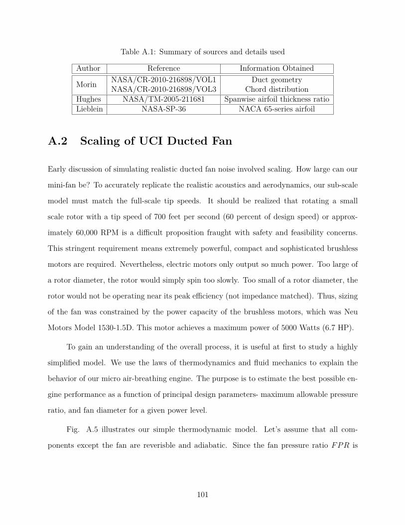
Table A.1: Summary of sources and details used
Author Reference Information Obtained
Morin NASA/CR-2010-216898/VOL1 Duct geometryNASA/CR-2010-216898/VOL3 Chord distribution
Hughes NASA/TM-2005-211681 Spanwise airfoil thickness ratioLieblein NASA-SP-36 NACA 65-series airfoil
A.2 Scaling of UCI Ducted Fan
Early discussion of simulating realistic ducted fan noise involved scaling. How large can our
mini-fan be? To accurately replicate the realistic acoustics and aerodynamics, our sub-scale
model must match the full-scale tip speeds. It should be realized that rotating a small
scale rotor with a tip speed of 700 feet per second (60 percent of design speed) or approx-
imately 60,000 RPM is a difficult proposition fraught with safety and feasibility concerns.
This stringent requirement means extremely powerful, compact and sophisticated brushless
motors are required. Nevertheless, electric motors only output so much power. Too large of
a rotor diameter, the rotor would simply spin too slowly. Too small of a rotor diameter, the
rotor would not be operating near its peak efficiency (not impedance matched). Thus, sizing
of the fan was constrained by the power capacity of the brushless motors, which was Neu
Motors Model 1530-1.5D. This motor achieves a maximum power of 5000 Watts (6.7 HP).
To gain an understanding of the overall process, it is useful at first to study a highly
simplified model. We use the laws of thermodynamics and fluid mechanics to explain the
behavior of our micro air-breathing engine. The purpose is to estimate the best possible en-
gine performance as a function of principal design parameters- maximum allowable pressure
ratio, and fan diameter for a given power level.
Fig. A.5 illustrates our simple thermodynamic model. Let’s assume that all com-
ponents except the fan are reverisble and adiabatic. Since the fan pressure ratio FPR is
101
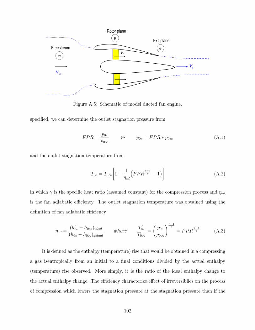
Rotor plane
Exit plane
e
R
Freestream
∞
Ve
Vi
V∞
Figure A.5: Schematic of model ducted fan engine.
specified, we can determine the outlet stagnation pressure from
FPR = p0e
p0∞↔ p0e = FPR ∗ p0∞ (A.1)
and the outlet stagnation temperature from
T0e = T0∞
[1 + 1
ηad
(FPR
γ−1γ − 1
)](A.2)
in which γ is the specific heat ratio (assumed constant) for the compression process and ηad
is the fan adiabatic efficiency. The outlet stagnation temperature was obtained using the
definition of fan adiabatic efficiency
ηad = (h′0e − h0∞)ideal(h0e − h0∞)actual
whereT ′0eT0∞
=(p0e
p0∞
) γ−1γ
= FPRγ−1γ (A.3)
It is defined as the enthalpy (temperature) rise that would be obtained in a compressing
a gas isentropically from an initial to a final conditions divided by the actual enthalpy
(temperature) rise observed. More simply, it is the ratio of the ideal enthalpy change to
the actual enthalpy change. The efficiency characterize effect of irreversiblies on the process
of compression which lowers the stagnation pressure at the stagnation pressure than if the
102
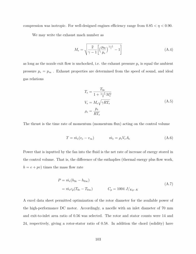
compression was isotropic. For well-designed engines efficiency range from 0.85 < η < 0.90.
We may write the exhaust mach number as
Me =
√√√√ 2γ − 1
[(p0e
pe
) γ−1γ − 1
](A.4)
as long as the nozzle exit flow is unchocked, i.e. the exhaust pressure pe is equal the ambient
pressure pe = p∞ . Exhaust properties are determined from the speed of sound, and ideal
gas relations
Te = T0e
1 + γ−12 M2
e
Ve = Me
√γRTe
ρe = peRTe
(A.5)
The thrust is the time rate of momentum (momentum flux) acting on the control volume
T = me(ve − v∞) me = ρeVeAe (A.6)
Power that is inputted by the fan into the fluid is the net rate of increase of energy stored in
the control volume. That is, the difference of the enthaplies (thermal energy plus flow work,
h = e+ pv) times the mass flow rate
P = me(h0e − h0∞)
= mecp(T0e − T0∞) Cp = 1004 J/Kg−K(A.7)
A excel data sheet permitted optimization of the rotor diameter for the available power of
the high-performance DC motor. Accordingly, a nacelle with an inlet diameter of 70 mm
and exit-to-inlet area ratio of 0.56 was selected. The rotor and stator counts were 14 and
24, respectively, giving a rotor-stator ratio of 0.58. In addition the chord (solidity) have
103
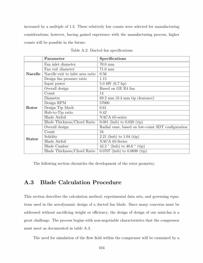
increased by a multiple of 1.3. These relatively low counts were selected for manufacturing
considerations; however, having gained experience with the manufacturing process, higher
counts will be possible in the future.
Table A.2: Ducted fan specifications
Parameter Specifications
Nacelle
Fan inlet diameter 70.0 mmFan exit diameter 71.0 mmNacelle exit to inlet area ratio 0.56Design fan pressure ratio 1.15Input power 5.0 kW (6.7 hp)
Rotor
Overall design Based on GE R4 fanCount 14Diameter 69.2 mm (0.4 mm tip clearance)Design RPM 57000Design Tip Mach 0.61Hub-to-Tip ratio 0.42Blade Airfoil NACA 65-seriesBlade Thickness/Chord Ratio 0.081 (hub) to 0.028 (tip)
Stator
Overall design Radial vane, based on low-count SDT configurationCount 24Solidity 2.21 (hub) to 1.04 (tip)Blade Airfoil NACA 65-SeriesBlade Camber 42.2 (hub) to 40.6 (tip)Blade Thickness/Chord Ratio 0.0707 (hub) to 0.0698 (tip)
The following section chronicles the development of the rotor geometry.
A.3 Blade Calculation Procedure
This section describes the calculation method, experimental data sets, and governing equa-
tions used in the aerodynamic design of a ducted fan blade. Since many concerns must be
addressed without sacrificing weight or efficiency, the design of design of our mini-fan is a
great challenge. The process begins with non-negotiable characteristics that the compressor
must meet as documented in table A.3.
The need for simulation of the flow field within the compressor will be examined by a
104
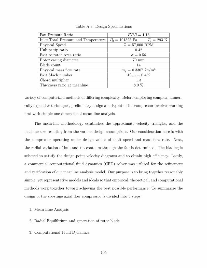
Table A.3: Design Specifications
Fan Pressure Ratio FPR = 1.15Inlet Total Pressure and Temperature P0 = 101325 Pa, T0 = 293 KPhysical Speed Ω = 57,000 RPMHub to tip ratio 0.42Exit to rotor Area ratio σ = 0.56Rotor casing diameter 70 mmBlade count 14Physical mass flow rate mp = 0.3307 kg/m3
Exit Mach number Mexit = 0.452Chord multiplier 1.3Thickness ratio at meanline 8.0 %
variety of computerized methods of differing complexity. Before employing complex, numeri-
cally expensive techniques, preliminary design and layout of the compressor involves working
first with simple one-dimensional mean-line analysis.
The mean-line methodology establishes the approximate velocity triangles, and the
machine size resulting from the various design assumptions. Our consideration here is with
the compressor operating under design values of shaft speed and mass flow rate. Next,
the radial variation of hub and tip contours through the fan is determined. The blading is
selected to satisfy the design-point velocity diagrams and to obtain high efficiency. Lastly,
a commercial computational fluid dynamics (CFD) solver was utilized for the refinement
and verification of our meanline analysis model. Our purpose is to bring together reasonably
simple, yet representative models and ideals so that empirical, theoretical, and computational
methods work together toward achieving the best possible performance. To summarize the
design of the six-stage axial flow compressor is divided into 3 steps:
1. Mean-Line Analysis
2. Radial Equilibrium and generation of rotor blade
3. Computational Fluid Dynamics
105
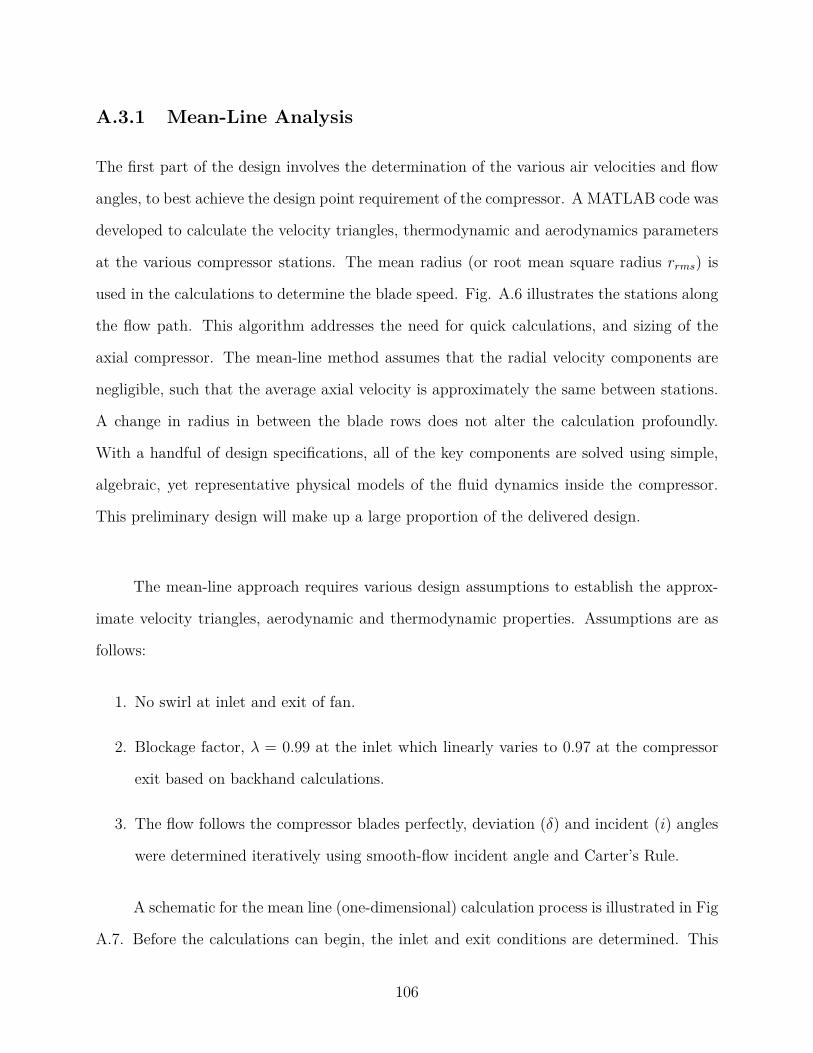
A.3.1 Mean-Line Analysis
The first part of the design involves the determination of the various air velocities and flow
angles, to best achieve the design point requirement of the compressor. A MATLAB code was
developed to calculate the velocity triangles, thermodynamic and aerodynamics parameters
at the various compressor stations. The mean radius (or root mean square radius rrms) is
used in the calculations to determine the blade speed. Fig. A.6 illustrates the stations along
the flow path. This algorithm addresses the need for quick calculations, and sizing of the
axial compressor. The mean-line method assumes that the radial velocity components are
negligible, such that the average axial velocity is approximately the same between stations.
A change in radius in between the blade rows does not alter the calculation profoundly.
With a handful of design specifications, all of the key components are solved using simple,
algebraic, yet representative physical models of the fluid dynamics inside the compressor.
This preliminary design will make up a large proportion of the delivered design.
The mean-line approach requires various design assumptions to establish the approx-
imate velocity triangles, aerodynamic and thermodynamic properties. Assumptions are as
follows:
1. No swirl at inlet and exit of fan.
2. Blockage factor, λ = 0.99 at the inlet which linearly varies to 0.97 at the compressor
exit based on backhand calculations.
3. The flow follows the compressor blades perfectly, deviation (δ) and incident (i) angles
were determined iteratively using smooth-flow incident angle and Carter’s Rule.
A schematic for the mean line (one-dimensional) calculation process is illustrated in Fig
A.7. Before the calculations can begin, the inlet and exit conditions are determined. This
106
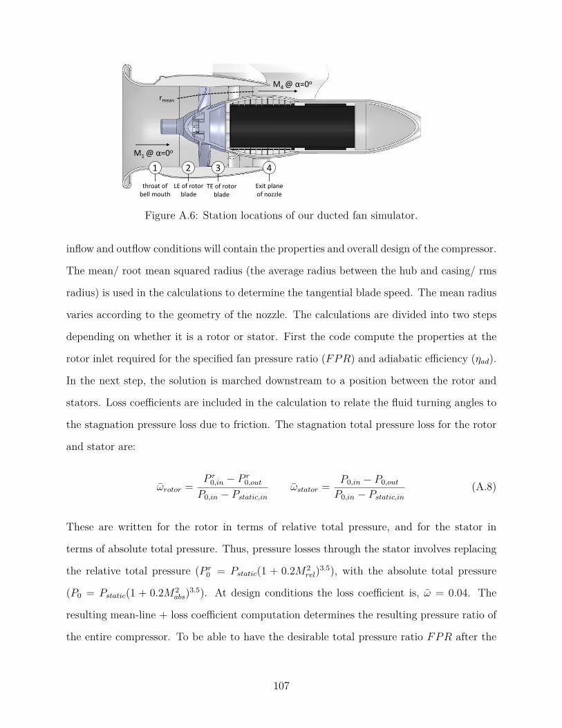
1 2 3 4
throat of bell mouth
LE of rotor blade
TE of rotor blade
Exit plane of nozzle
M1 @ α=0o
M4 @ α=0o
rmean
Figure A.6: Station locations of our ducted fan simulator.
inflow and outflow conditions will contain the properties and overall design of the compressor.
The mean/ root mean squared radius (the average radius between the hub and casing/ rms
radius) is used in the calculations to determine the tangential blade speed. The mean radius
varies according to the geometry of the nozzle. The calculations are divided into two steps
depending on whether it is a rotor or stator. First the code compute the properties at the
rotor inlet required for the specified fan pressure ratio (FPR) and adiabatic efficiency (ηad).
In the next step, the solution is marched downstream to a position between the rotor and
stators. Loss coefficients are included in the calculation to relate the fluid turning angles to
the stagnation pressure loss due to friction. The stagnation total pressure loss for the rotor
and stator are:
ωrotor =P r
0,in − P r0,out
P0,in − Pstatic,inωstator = P0,in − P0,out
P0,in − Pstatic,in(A.8)
These are written for the rotor in terms of relative total pressure, and for the stator in
terms of absolute total pressure. Thus, pressure losses through the stator involves replacing
the relative total pressure (P r0 = Pstatic(1 + 0.2M2
rel)3.5), with the absolute total pressure
(P0 = Pstatic(1 + 0.2M2abs)3.5). At design conditions the loss coefficient is, ω = 0.04. The
resulting mean-line + loss coefficient computation determines the resulting pressure ratio of
the entire compressor. To be able to have the desirable total pressure ratio FPR after the
107
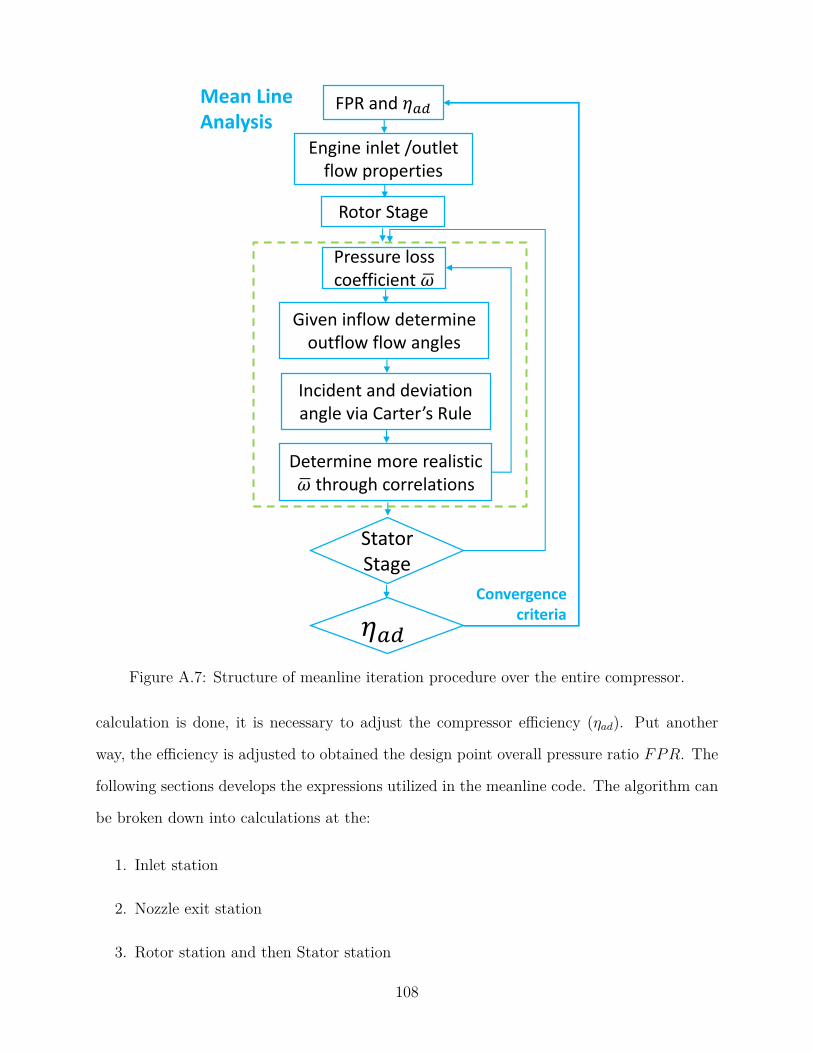
FPR and 𝜂𝑎𝑑
Engine inlet /outlet flow properties
Rotor Stage
Pressure loss coefficient ഥ𝜔
Given inflow determine outflow flow angles
Incident and deviation angle via Carter’s Rule
Determine more realistic ഥ𝜔 through correlations
Stator Stage
𝜂𝑎𝑑
Mean Line Analysis
Convergence criteria
Figure A.7: Structure of meanline iteration procedure over the entire compressor.
calculation is done, it is necessary to adjust the compressor efficiency (ηad). Put another
way, the efficiency is adjusted to obtained the design point overall pressure ratio FPR. The
following sections develops the expressions utilized in the meanline code. The algorithm can
be broken down into calculations at the:
1. Inlet station
2. Nozzle exit station
3. Rotor station and then Stator station
108
Inflow Calculation Steps
Given the casing and hub profile, the root mean squared mean radius is
rrms =(r2case + r2
hub
2
) 12
(A.9)
the physical area
Aphy = π(r2case − r2
hub) (A.10)
velocity of rotor at pitch line
Urms = rrmsπRPM
30 (A.11)
the mach number at station 1 and 2 is obtained from
mp
√T0
P0Aphysλ=√γ
R
[M
(1 + γ−12 M2)
γ+12(γ−1)
](A.12)
For a given total temperature/pressure (isotropic through inlet), and blockage ratio- the
Mach number is solved implicitly. λ is the blockage factor- the ratio of effective flow area to
physical area.
λ =(
1− AeffAphy
)x100%
AphyAphyAeff
Figure A.8: Casing boundary layer growth and modeling.
109
This factor accounts for the area losses generated by the end walls due to the growth of
the casing boundary layer. The formation, and development of these boundary layer block
or reduce the physical area in which the flow can travel. A cartoon of end wall loses can
be view in Fig A.8. Calculation of the inlet Mach number allows for determination of static
thermodynamic variables
Tstatic = T0
1 + γ+12 M2 pstatic = P0
(1 + γ+12 M2)
γγ−1
(A.13)
a =√γRTstatic c = Ma ρ = pstatic
RTstaticρ0 = ρ
(1 + γ − 1
2 M2) γγ−1
where a,c are the local speed of sound, and absolute velocity (flow velocity in the absolute
frame of reference), respectively.
Nozzle Exit Calculation Steps
Overall temperature ratio
OTR = FPRγ−1γ − 1
ηad+ 1 (A.14)
where ηad is the adiabatic efficiency. It first value is approximated, and then a new value is
calculated to adjust the approximated first value. This process iterates until ηad converges
as illustrated in Fig. A.7. The total temperature for last stage (station 4) is
T0[4] = OTR ∗ T0[2] (A.15)
the shaft work that must be supplied to drive the fan normalized by fan angular velocity is
a function of the flow turning (∆(rcu)) across the rotor in the absolute reference frame
∆(rCu) = W
ω= Cp∆Tπ ∗RPM/30 (A.16)
110
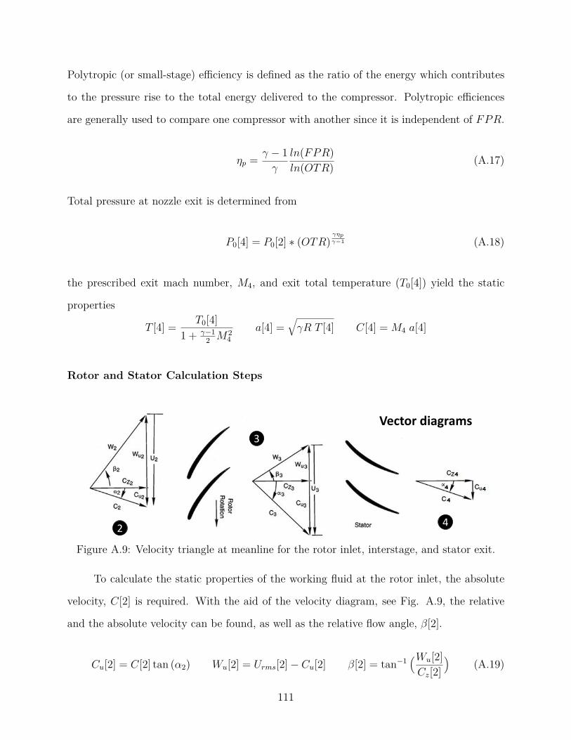
Polytropic (or small-stage) efficiency is defined as the ratio of the energy which contributes
to the pressure rise to the total energy delivered to the compressor. Polytropic efficiences
are generally used to compare one compressor with another since it is independent of FPR.
ηp = γ − 1γ
ln(FPR)ln(OTR) (A.17)
Total pressure at nozzle exit is determined from
P0[4] = P0[2] ∗ (OTR)γηpγ−1 (A.18)
the prescribed exit mach number, M4, and exit total temperature (T0[4]) yield the static
properties
T [4] = T0[4]1 + γ−1
2 M24
a[4] =√γR T [4] C[4] = M4 a[4]
Rotor and Stator Calculation Steps
2
3
4
Vector diagrams
Figure A.9: Velocity triangle at meanline for the rotor inlet, interstage, and stator exit.
To calculate the static properties of the working fluid at the rotor inlet, the absolute
velocity, C[2] is required. With the aid of the velocity diagram, see Fig. A.9, the relative
and the absolute velocity can be found, as well as the relative flow angle, β[2].
Cu[2] = C[2] tan (α2) Wu[2] = Urms[2]− Cu[2] β[2] = tan−1(Wu[2]Cz[2]
)(A.19)
111
The properties of the gas as seen by the rotor in the relative frame of reference are computed
from the static properties of the gas, which do not change when transferring between reference
frame.
W [2] = Cz[2]cos (β[2]) Mrel = W [2]
a[2] P r0 [2] = Pstatic[2]
(1 + γ − 1
2 M2rel
) γγ−1 (A.20)
To move from the rotor-inlet towards the outlet of the rotor the rotor exit absolute flow
angles (α[3]) must be known. The rotor exit flow angle determines the incident (i) and
deviation (δ) angles and loss coefficient (ω) which also depends on i, δ. This highly coupled
system is solved using iteration. As illustrated in Fig. A.7 this procedure is composed of 3
main sub-calculations:
1. Determination of outflow angles
2. Determination of incident and deviation angles
3. Determination of more realistic loss coefficient ω
1. Absolute flow angle
The absolute mach number at the rotor exit (station 3) is
mp
√T0[3]
P0[3]Aphys[3] λ[3] =√γ
R
[M
(1 + γ−12 M2)
γ+12(γ−1)
](A.21)
with static properties
Tstatic[3] = T0[3]1 + γ−1
2 M [3]2a[3] =
√γRTstatic[3] c[3] = M [3] a[3]
112
For the specified FPR the flow properties are
Cu[3] = ∆(rCu) + rrms[2]Cu[2]rrms[3] Wu[3] = Urms[3]− Cu[3] α[3] = sin−1(Cu[3]
C[3] )
For typical multistage compressor design, the above step require iteration where a initial
guess of the rotor exit absolute flow angle is made and checked until the associated stage
work (∆rCu) converge to the required for design- since the hub geometry is unknown. Here,
knowing the duct geometry simplifies the computation. For the absolute flow angle (α) the
properties at the end of rotor are
Cz[3] = C[3] cos(α[3]) W [3] =√Cz[3]2 +Wu[3]2 Mrel = W [3]
a[3]
The relative total pressure and static pressure is
P r0 [3] = P r
0 [2]− ωrotor(P r0 [2]− Pstatic[2]) Pstatic[3] = P r
0 [3](1 + γ−1
2 Mrel[3]2)γγ−1
Note the stagnation pressure loss coefficient ω depends on i, δ. For the first loop, we use the
design point loss coeffient ω = 0.4. Thus, iteration is required to get an realistic coefficient.
2. Incidence and deviation angle
For internal flows, the incident angle (i) is comparable to the angle of attack (α). The
incidence angle is the difference between the blade angle and the flow angle as sketched in
right illustration in Fig. A.12. The deviation angle is the difference between the air angle and
the mean line angle at the trailing edge. Imagine a cascade operating under design conditions
draw in the right panel in Fig A.12. As the inlet flow angle βi increase the outflow angle βii
remains essentially constant until the inflow is too steep for the flow to follow the surface
of the airfoil. Boundary layer separation takes place due to the adverse pressure gradient
on the suction surface of the blades. A separation region forms, increasing total pressure
113
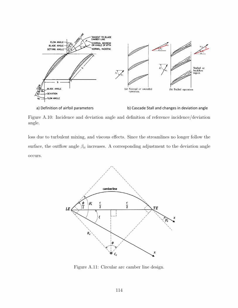
a) Definition of airfoil parameters b) Cascade Stall and changes in deviation angle
𝛿
Figure A.10: Incidence and deviation angle and definition of reference incidence/deviationangle.
loss due to turbulent mixing, and viscous effects. Since the streamlines no longer follow the
surface, the outflow angle βii increases. A corresponding adjustment to the deviation angle
occurs.
Figure A.11: Circular arc camber line design.
114
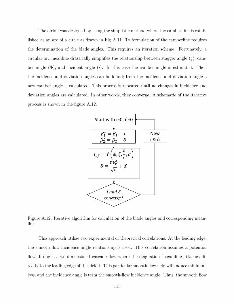
The airfoil was designed by using the simplistic method where the camber line is estab-
lished as an arc of a circle as drawn in Fig A.11. To formulation of the camberline requires
the determination of the blade angles. This requires an iteration scheme. Fortunately, a
circular arc meanline drastically simplifies the relationship between stagger angle (ξ), cam-
ber angle (Φ), and incident angle (i). In this case the camber angle is estimated. Then
the incidence and deviation angles can be found; from the incidence and deviation angle a
new camber angle is calculated. This process is repeated until no changes in incidence and
deviation angles are calculated. In other words, they converge. A schematic of the iterative
process is shown in the figure A.12.
Start with i=0, δ=0
𝛽1∗ = 𝛽1 − 𝑖
𝛽2∗ = 𝛽2 − 𝛿
𝑖𝑠𝑓 = 𝑓 𝜙, 𝜉,𝑡
𝑐, 𝜎
𝛿 =𝑚𝜙
𝜎+ 𝑋
𝑖 𝑎𝑛𝑑 𝛿
converge?
New i & δ
Figure A.12: Iterative algorithm for calculation of the blade angles and corresponding mean-line.
This approach utilize two experimental or theoretical correlations. At the leading edge,
the smooth flow incidence angle relationship is used. This correlation assumes a potential
flow through a two-dimensional cascade flow where the stagnation streamline attaches di-
rectly to the leading edge of the airfoil. This particular smooth flow field will induce minimum
loss, and the incidence angle is term the smooth-flow incidence angle. Thus, the smooth flow
115
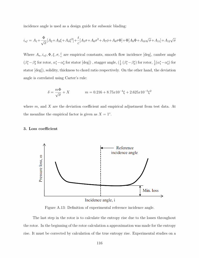
incidence angle is used as a design guide for subsonic blading:
isf = A1+ Φ√σ
[A2+A3ξ+A4ξ2]+ t
c[A5σ+A6σ
2+A7φ+A8σΦ]+Φ[A9Φ+A10√σ+A11]+A12
√σ
Where An, isf ,Φ, ξ, σ, tc are empirical constants, smooth flow incidence [deg], camber angle
(β∗1−β∗2 for rotor, α∗1−α∗2 for stator [deg]) , stagger angle, (12 (β∗1−β∗2) for rotor, 1
2(α∗1−α∗2) for
stator [deg]), solidity, thickness to chord ratio respectively. On the other hand, the deviation
angle is correlated using Carter’s rule:
δ = mΦ√σ
+X m = 0.216 + 8.75x10⁻⁴ξ + 2.625x10⁻⁵ξ2
where m, and X are the deviation coefficient and empirical adjustment from test data. At
the meanline the empirical factor is given as X = 1.
3. Loss coefficient
Figure A.13: Definition of experimental reference incidence angle.
The last step in the rotor is to calculate the entropy rise due to the losses throughout
the rotor. In the beginning of the rotor calculation a approximation was made for the entropy
rise. It must be corrected by calculation of the true entropy rise. Experimental studies on a
116
given cascade, format their results according to a reference incidence (iref ) when testing at
different inflow flow angles. The total pressure loss coefficient depends on incidence angle.
Mirroring drag, the loss coefficient ω will increase for both positive and negative incidence
angles. The minimum total pressure loss occurs at the reference incidence angle according
to Fig. A.13. In NASA report N65-23345, Chapter VI- “Experimental Flow in 2D Cascade",
Lieblin proposed the correlation for reference incidence angle as
iref = (Ki)sh(Ki)t(i0)10 + nΦ
Where Ksh and Kt are corrections that accounts for blade shape and thickness. For a NACA
65-Series Ksh = 1.0. and the thickness correction Kt, is determined from an least square
cubic curve fit as:
(Ki)t = −0.0214 + 19.17(t
c
)− 122.3
(t
c
)2
+ 312.5(t
c
)3
Φ is the camber, (i0)10 is the reference incidence angle for a zero camber 10% thick NACA
65-A10, and n is the incidence angle slope factor. Linear regression of the data set yields:
(io)10 = (0.0324− 0.0674σ) + (−0.002364 + 0.0913σ)β1 + (1.6x10⁻⁵ − 2.38x10⁻⁴σ)β21
n = (−0.063 + 0.02274σ) + (−0.0035 + 0.0029σ)β1 − (3.79x10⁻⁵ + 1.11x10⁻⁵σ)β21
Graphs of the thickness correction (Ki)t, zero-camber incidence angle (io)10, and the inci-
dence angle slope factor n are plotted in Fig. A.14-A.15.
Lieblin recommend a similar structure to that of the reference deviation angle. The
reference deviation angle (δref ) is
δref = (Kδ)sh(Kδ)t(δ0)10 +mΦ
117
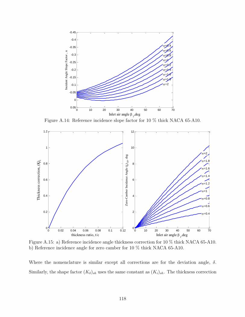
0 10 20 30 40 50 60 70
-0.45
-0.4
-0.35
-0.3
-0.25
-0.2
-0.15
-0.1
-0.05
0
0.05
=0.4
=0.6
=0.8
=1
=1.2
=1.4
=1.6
=1.8
=2
Inlet air angle 1,deg
Inci
den
t A
ng
le S
lop
e F
acto
r ,
n
Figure A.14: Reference incidence slope factor for 10 % thick NACA 65-A10.
0 10 20 30 40 50 60 700
2
4
6
8
10
12
=0.4
=0.6
=0.8
=1
=1.2
=1.4
=1.6
=1.8
=2
Inlet air angle 1,deg
Zer
o-C
amber
Inci
den
ce A
ngle
(i 0
) 10,
deg
0 0.02 0.04 0.06 0.08 0.1 0.120
0.2
0.4
0.6
0.8
1
1.2
thickness ratio, t/c
Th
ick
ness
co
rrecti
on
, (K
i)t
Figure A.15: a) Reference incidence angle thickness correction for 10 % thick NACA 65-A10.b) Reference incidence angle for zero camber for 10 % thick NACA 65-A10.
Where the nomenclature is similar except all corrections are for the deviation angle, δ.
Similarly, the shape factor (Kδ)sh uses the same constant as (Ki)sh. The thickness correction
118
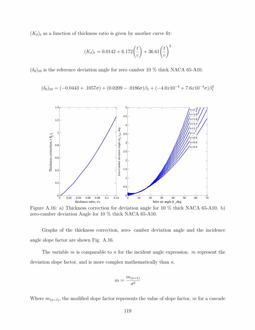
(Kδ)t as a function of thickness ratio is given by another curve fit:
(Kδ)t = 0.0142 + 6.172(t
c
)+ 36.61
(t
c
)2
(δ0)10 is the reference deviation angle for zero camber 10 % thick NACA 65-A10.
(δ0)10 = (−0.0443 + .1057σ) + (0.0209− .0186σ)β1 + (−4.0x10⁻⁴ + 7.6x10⁻⁴σ)β21
0 0.02 0.04 0.06 0.08 0.1 0.120
0.2
0.4
0.6
0.8
1
1.2
1.4
thickness ratio, t/c
Th
ick
ness
co
rrecti
on
, (
K )
t
0 10 20 30 40 50 60 700
0.5
1
1.5
2
2.5
3
3.5
4
4.5
5
=0.4
=0.6
=0.8
=1
=1.2
=1.4
=1.6
=1.8
=2
Inlet air angle 1,deg
Zer
o-C
amb
er d
evia
tio
n A
ng
le (
0 )
10,
deg
Figure A.16: a) Thickness correction for deviation angle for 10 % thick NACA 65-A10. b)zero-camber deviation Angle for 10 % thick NACA 65-A10.
Graphs of the thickness correction, zero- camber deviation angle and the incidence
angle slope factor are shown Fig. A.16.
The variable m is comparable to n for the incident angle expression. m represent the
deviation slope factor, and is more complex mathematically than n.
m = m(σ=1)
σb
Where m(σ=1), the modified slope factor represents the value of slope factor, m for a cascade
119
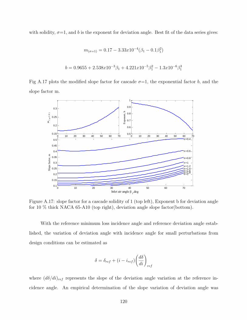
with solidity, σ=1, and b is the exponent for deviation angle. Best fit of the data series gives:
m(σ=1) = 0.17− 3.33x10⁻⁴(β1 − 0.1β21)
b = 0.9655 + 2.538x10⁻³β1 + 4.221x10⁻⁵β21 − 1.3x10⁻⁶β3
1
Fig A.17 plots the modified slope factor for cascade σ=1, the exponential factor b, and the
slope factor m.
0 10 20 30 40 50 60 700.15
0.2
0.25
0.3
m (
=
1.0
)
0 10 20 30 40 50 60 700.5
0.6
0.7
0.8
0.9
1
Exponen
t, b
0 10 20 30 40 50 60 700.1
0.15
0.2
0.25
0.3
0.35
0.4
0.45
0.5 =0.4
=0.6
=0.8
=1
=1.2=1.4=1.6=1.8=2
Inlet air angle 1,deg
Slo
pe
fact
or,
m
Figure A.17: slope factor for a cascade solidity of 1 (top left), Exponent b for deviation anglefor 10 % thick NACA 65-A10 (top right), deviation angle slope factor(bottom).
With the reference minimum loss incidence angle and reference deviation angle estab-
lished, the variation of deviation angle with incidence angle for small perturbations from
design conditions can be estimated as
δ = δref + (i− iref )(dδ
di
)ref
where (dδ/di)ref represents the slope of the deviation angle variation at the reference in-
cidence angle. An empirical determination of the slope variation of deviation angle was
120
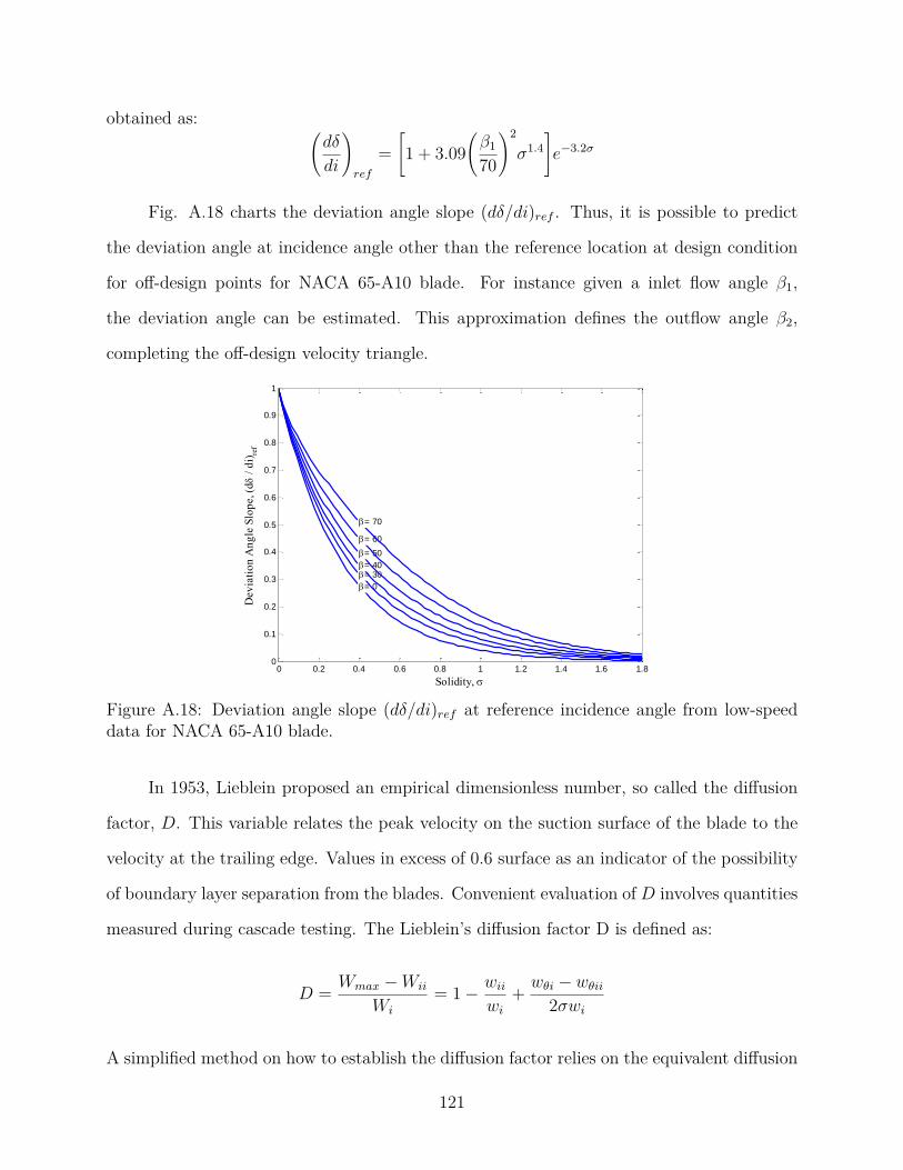
obtained as: (dδ
di
)ref
=[1 + 3.09
(β1
70
)2
σ1.4]e−3.2σ
Fig. A.18 charts the deviation angle slope (dδ/di)ref . Thus, it is possible to predict
the deviation angle at incidence angle other than the reference location at design condition
for off-design points for NACA 65-A10 blade. For instance given a inlet flow angle β1,
the deviation angle can be estimated. This approximation defines the outflow angle β2,
completing the off-design velocity triangle.
0 0.2 0.4 0.6 0.8 1 1.2 1.4 1.6 1.80
0.1
0.2
0.3
0.4
0.5
0.6
0.7
0.8
0.9
1
= 0
= 30= 40
= 50
= 60
= 70
Solidity,
Dev
iati
on
An
gle
Slo
pe, (d
/
di)
ref
Figure A.18: Deviation angle slope (dδ/di)ref at reference incidence angle from low-speeddata for NACA 65-A10 blade.
In 1953, Lieblein proposed an empirical dimensionless number, so called the diffusion
factor, D. This variable relates the peak velocity on the suction surface of the blade to the
velocity at the trailing edge. Values in excess of 0.6 surface as an indicator of the possibility
of boundary layer separation from the blades. Convenient evaluation of D involves quantities
measured during cascade testing. The Lieblein’s diffusion factor D is defined as:
D = Wmax −Wii
Wi
= 1− wiiwi
+ wθi − wθii2σwi
A simplified method on how to establish the diffusion factor relies on the equivalent diffusion
121
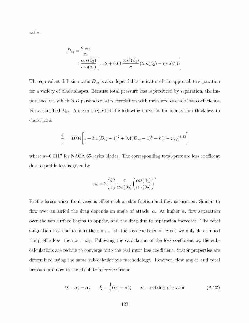
ratio:
Deq = cmaxc2
= cos(β2)cos(β1)
[1.12 + 0.61cos
2(β1)σ
(tan(β2)− tan(β1))]
The equivalent diffusion ratio Deq is also dependable indicator of the approach to separation
for a variety of blade shapes. Because total pressure loss is produced by separation, the im-
portance of Leiblein’s D parameter is its correlation with measured cascade loss coefficients.
For a specified Deq, Aungier suggested the following curve fit for momentum thickness to
chord ratio
θ
c= 0.004
[1 + 3.1(Deq − 1)2 + 0.4(Deq − 1)8 + k(i− iref )1.43
]
where a=0.0117 for NACA 65-series blades. The corresponding total-pressure loss coefficent
due to profile loss is given by
ωp = 2(θ
c
)σ
cos(β2)
(cos(β1)cos(β2)
)2
Profile losses arises from viscous effect such as skin friction and flow separation. Similar to
flow over an airfoil the drag depends on angle of attack, α. At higher α, flow separation
over the top surface begins to appear, and the drag due to separation increases. The total
stagnation loss coefficent is the sum of all the loss coefficients. Since we only determined
the profile loss, then ω = ωp. Following the calculation of the loss coefficient ωp the sub-
calculations are redone to converge onto the real rotor loss coefficient. Stator properties are
determined using the same sub-calculations methodology. However, flow angles and total
pressure are now in the absolute reference frame
Φ = α∗1 − α∗2 ξ = 12(α∗1 + α∗2) σ = solidity of stator (A.22)
122

that is, every relative flow angle is replaced by the absolute flow angle in the correlations,
i.e. β1 → α1, β2 → α2. As shown in Fig. A.7, the total pressure loss-coefficient for the
stator ωstator is computed by recursion. Since the stator blades were already designed during
a previous investigation, to simplify and ease calculations it was assumed no total pressure
loss occurred across the stators, i.e. P0[3] = P0[4]. Thus, the static pressure at the exit is
Pstatic[4] = P0[4](1 + γ − 1
2 M [4]2) γγ−1 (A.23)
A.4 Radial Equilibrium and Blade Stacking
So far we restricted our attention to the meanline. To design a efficient fan, the radial
variations from the rotor hub to tip must be calculated. Thus, it is necessary to take into
account radial varation in blade speed, axial velocity (cz), and tangential velocity (cθ). The
design of the rotor blades is obtained from the energy equation, with the assumption that
the radial gradient of the entropy and the stagnation enthaply are zero
d
dr(c2z) = −1
r2d
dr(rcθ)2
The above expression couples the axial velocity component and the angular momentum rcθ.
The velocity distributions must satisfy this relationship at the entrance and exit of the rotor.
In order to provide uniform flow at the exit of the fan, it is necessary to evenly distribute
the work input along the radial length of a rotor. Thus, to keep the work constant, the
product r∆cθ must be constant with radius. The product r∆cθ(r) distribution is regarded
as a design choice that will influence the blade twist. One configuration that satisfy this
requirement is the “constant reaction” distribution
rcθ = ar2 + b (A.24)
123
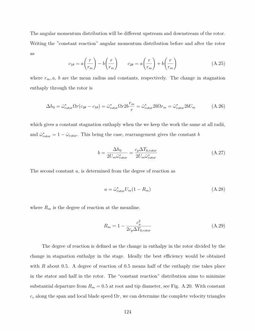
The angular momentum distribution will be different upstream and downstream of the rotor.
Writing the ”constant reaction” angular momentum distribution before and after the rotor
as
c1θ = a
(r
rm
)− b
(r
rm
)c2θ = a
(r
rm
)+ b
(r
rm
)(A.25)
where rm, a, b are the mean radius and constants, respectively. The change in stagnation
enthaply through the rotor is
∆h0 = ω∗rotorΩr(c2θ − c1θ) = ω∗rotorΩr2brmr
= ω∗rotor2bΩrm = ω∗rotor2bUm (A.26)
which gives a constant stagnation enthaply when the we keep the work the same at all radii,
and ω∗rotor = 1− ωrotor. This being the case, rearrangement gives the constant b
b = ∆h0
2Umω∗rotor= cp∆T0,rotor
2Umω∗rotor(A.27)
The second constant a, is determined from the degree of reaction as
a = ω∗rotorUm(1−Rm) (A.28)
where Rm is the degree of reaction at the meanline.
Rm = 1− c2u
2cp∆T0,rotor(A.29)
The degree of reaction is defined as the change in enthalpy in the rotor divided by the
change in stagnation enthalpy in the stage. Ideally the best efficiency would be obtained
with R about 0.5. A degree of reaction of 0.5 means half of the enthaply rise takes place
in the stator and half in the rotor. The “constant reaction” distribution aims to minimize
substantial departure from Rm = 0.5 at root and tip diameter, see Fig. A.20. With constant
cz along the span and local blade speed Ωr, we can determine the complete velocity triangles
124
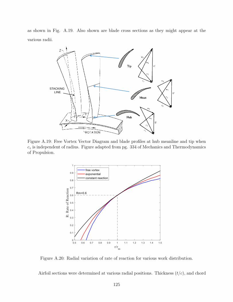
as shown in Fig. A.19. Also shown are blade cross sections as they might appear at the
various radii.
STACKING
LINE
Figure A.19: Free Vortex Vector Diagram and blade profiles at hub meanline and tip whencz is independent of radius. Figure adapted from pg. 334 of Mechanics and Thermodynamicsof Propulsion.
Figure A.20: Radial variation of rate of reaction for various work distribution.
Airfoil sections were determined at various radial positions. Thickness (t/c), and chord
125
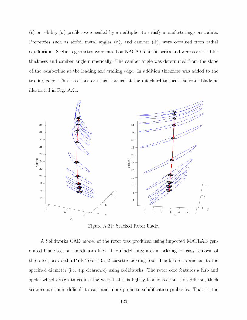
(c) or solidity (σ) profiles were scaled by a multiplier to satisfy manufacturing constraints.
Properties such as airfoil metal angles (β), and camber (Φ), were obtained from radial
equilibrium. Sections geometry were based on NACA 65-airfoil series and were corrected for
thickness and camber angle numerically. The camber angle was determined from the slope
of the camberline at the leading and trailing edge. In addition thickness was added to the
trailing edge. These sections are then stacked at the midchord to form the rotor blade as
illustrated in Fig. A.21.
Figure A.21: Stacked Rotor blade.
A Solidworks CAD model of the rotor was produced using imported MATLAB gen-
erated blade-section coordinates files. The model integrates a lockring for easy removal of
the rotor, provided a Park Tool FR-5.2 cassette lockring tool. The blade tip was cut to the
specified diameter (i.e. tip clearance) using Solidworks. The rotor core features a hub and
spoke wheel design to reduce the weight of this lightly loaded section. In addition, thick
sections are more difficult to cast and more prone to solidification problems. That is, the
126
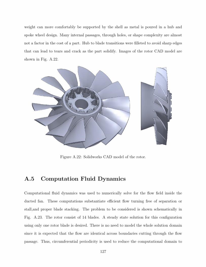
weight can more comfortably be supported by the shell as metal is poured in a hub and
spoke wheel design. Many internal passages, through holes, or shape complexity are almost
not a factor in the cost of a part. Hub to blade transitions were filleted to avoid sharp edges
that can lead to tears and crack as the part solidify. Images of the rotor CAD model are
shown in Fig. A.22.
Figure A.22: Solidworks CAD model of the rotor.
A.5 Computation Fluid Dynamics
Computational fluid dynamics was used to numerically solve for the flow field inside the
ducted fan. These computations substantiate efficient flow turning free of separation or
stall,and proper blade stacking. The problem to be considered is shown schematically in
Fig. A.23. The rotor consist of 14 blades. A steady state solution for this configuration
using only one rotor blade is desired. There is no need to model the whole solution domain
since it is expected that the flow are identical across boundaries cutting through the flow
passage. Thus, circumferential periodicity is used to reduce the computational domain to
127
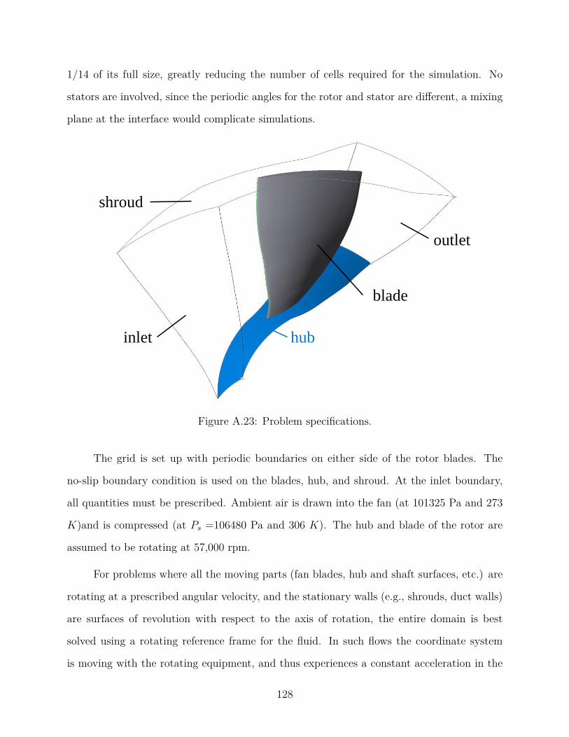
1/14 of its full size, greatly reducing the number of cells required for the simulation. No
stators are involved, since the periodic angles for the rotor and stator are different, a mixing
plane at the interface would complicate simulations.
inlet
outlet
hub
blade
shroud
Figure A.23: Problem specifications.
The grid is set up with periodic boundaries on either side of the rotor blades. The
no-slip boundary condition is used on the blades, hub, and shroud. At the inlet boundary,
all quantities must be prescribed. Ambient air is drawn into the fan (at 101325 Pa and 273
K)and is compressed (at Ps =106480 Pa and 306 K). The hub and blade of the rotor are
assumed to be rotating at 57,000 rpm.
For problems where all the moving parts (fan blades, hub and shaft surfaces, etc.) are
rotating at a prescribed angular velocity, and the stationary walls (e.g., shrouds, duct walls)
are surfaces of revolution with respect to the axis of rotation, the entire domain is best
solved using a rotating reference frame for the fluid. In such flows the coordinate system
is moving with the rotating equipment, and thus experiences a constant acceleration in the
128
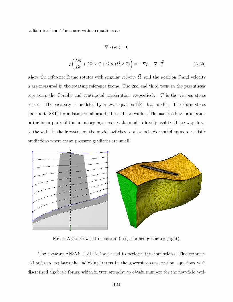
radial direction. The conservation equations are
∇ · (ρu) = 0
ρ
(D~u
Dt+ 2~Ω× ~u+ ~Ω× (~Ω× ~x)
)= −∇p+∇ · ¯T (A.30)
where the reference frame rotates with angular velocity ~Ω, and the position ~x and velocity
~u are measured in the rotating reference frame. The 2nd and third term in the parenthesis
represents the Coriolis and centripetal acceleration, respectively. ¯T is the viscous stress
tensor. The viscosity is modeled by a two equation SST k-ω model. The shear stress
transport (SST) formulation combines the best of two worlds. The use of a k-ω formulation
in the inner parts of the boundary layer makes the model directly usable all the way down
to the wall. In the free-stream, the model switches to a k-ε behavior enabling more realistic
predictions where mean pressure gradients are small.
Figure A.24: Flow path coutours (left), meshed geometry (right).
The software ANSYS FLUENT was used to perform the simulations. This commer-
cial software replaces the individual terms in the governing conservation equations with
discretized algebraic forms, which in turn are solve to obtain numbers for the flow-field vari-
129
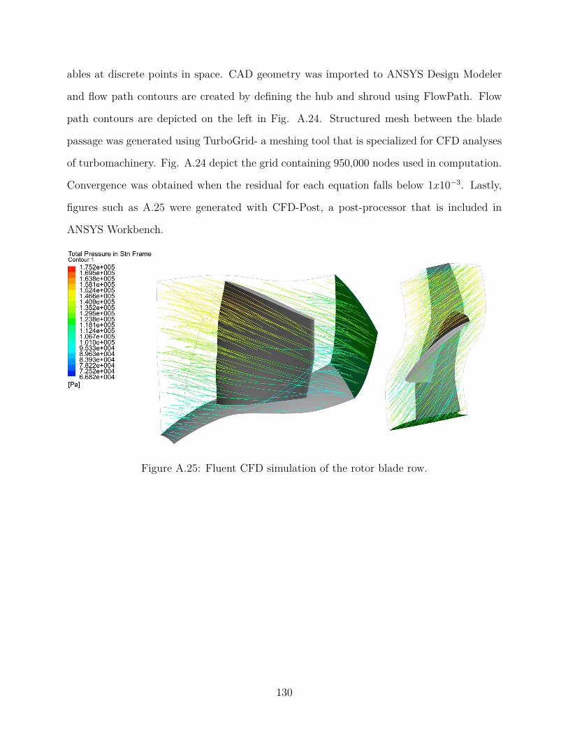
ables at discrete points in space. CAD geometry was imported to ANSYS Design Modeler
and flow path contours are created by defining the hub and shroud using FlowPath. Flow
path contours are depicted on the left in Fig. A.24. Structured mesh between the blade
passage was generated using TurboGrid- a meshing tool that is specialized for CFD analyses
of turbomachinery. Fig. A.24 depict the grid containing 950,000 nodes used in computation.
Convergence was obtained when the residual for each equation falls below 1x10⁻³. Lastly,
figures such as A.25 were generated with CFD-Post, a post-processor that is included in
ANSYS Workbench.
Figure A.25: Fluent CFD simulation of the rotor blade row.
130
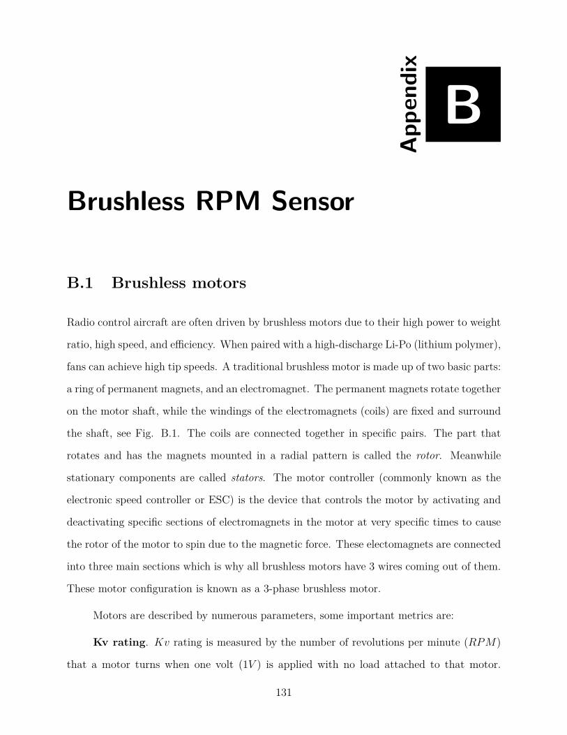
B
App
endi
x
Brushless RPM Sensor
B.1 Brushless motors
Radio control aircraft are often driven by brushless motors due to their high power to weight
ratio, high speed, and efficiency. When paired with a high-discharge Li-Po (lithium polymer),
fans can achieve high tip speeds. A traditional brushless motor is made up of two basic parts:
a ring of permanent magnets, and an electromagnet. The permanent magnets rotate together
on the motor shaft, while the windings of the electromagnets (coils) are fixed and surround
the shaft, see Fig. B.1. The coils are connected together in specific pairs. The part that
rotates and has the magnets mounted in a radial pattern is called the rotor. Meanwhile
stationary components are called stators. The motor controller (commonly known as the
electronic speed controller or ESC) is the device that controls the motor by activating and
deactivating specific sections of electromagnets in the motor at very specific times to cause
the rotor of the motor to spin due to the magnetic force. These electomagnets are connected
into three main sections which is why all brushless motors have 3 wires coming out of them.
These motor configuration is known as a 3-phase brushless motor.
Motors are described by numerous parameters, some important metrics are:
Kv rating. Kv rating is measured by the number of revolutions per minute (RPM)
that a motor turns when one volt (1V ) is applied with no load attached to that motor.
131
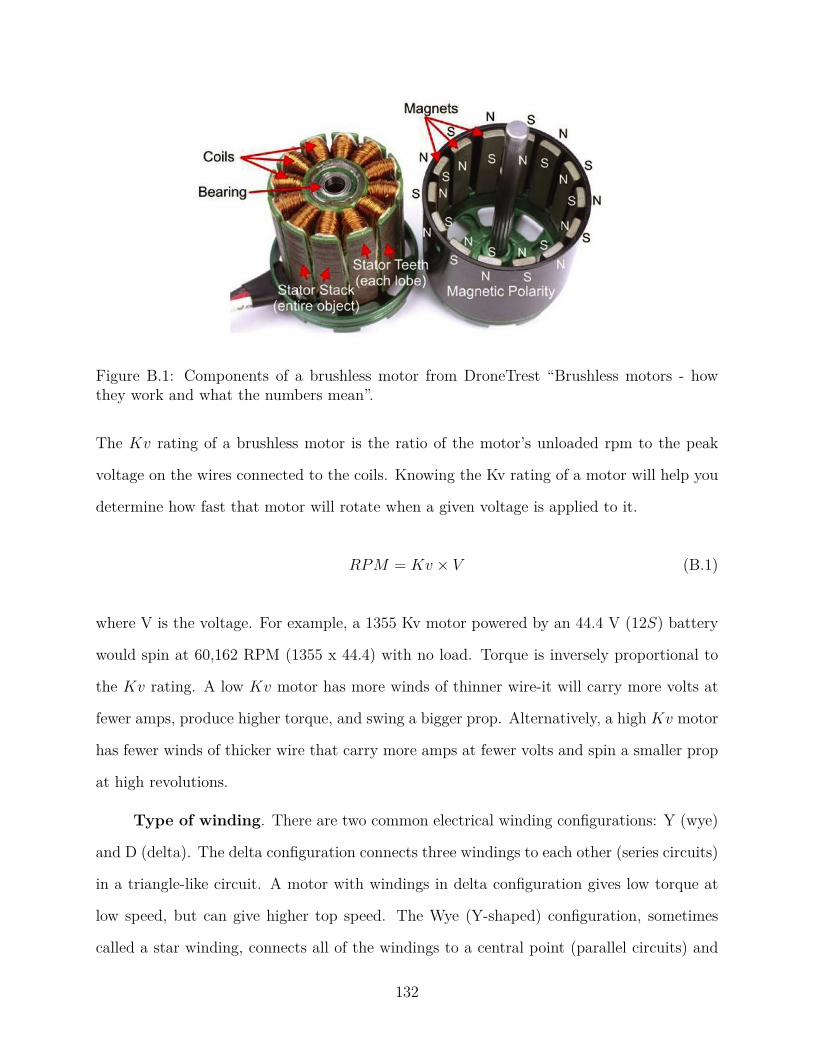
Figure B.1: Components of a brushless motor from DroneTrest “Brushless motors - howthey work and what the numbers mean”.
The Kv rating of a brushless motor is the ratio of the motor’s unloaded rpm to the peak
voltage on the wires connected to the coils. Knowing the Kv rating of a motor will help you
determine how fast that motor will rotate when a given voltage is applied to it.
RPM = Kv × V (B.1)
where V is the voltage. For example, a 1355 Kv motor powered by an 44.4 V (12S) battery
would spin at 60,162 RPM (1355 x 44.4) with no load. Torque is inversely proportional to
the Kv rating. A low Kv motor has more winds of thinner wire-it will carry more volts at
fewer amps, produce higher torque, and swing a bigger prop. Alternatively, a high Kv motor
has fewer winds of thicker wire that carry more amps at fewer volts and spin a smaller prop
at high revolutions.
Type of winding. There are two common electrical winding configurations: Y (wye)
and D (delta). The delta configuration connects three windings to each other (series circuits)
in a triangle-like circuit. A motor with windings in delta configuration gives low torque at
low speed, but can give higher top speed. The Wye (Y-shaped) configuration, sometimes
called a star winding, connects all of the windings to a central point (parallel circuits) and
132
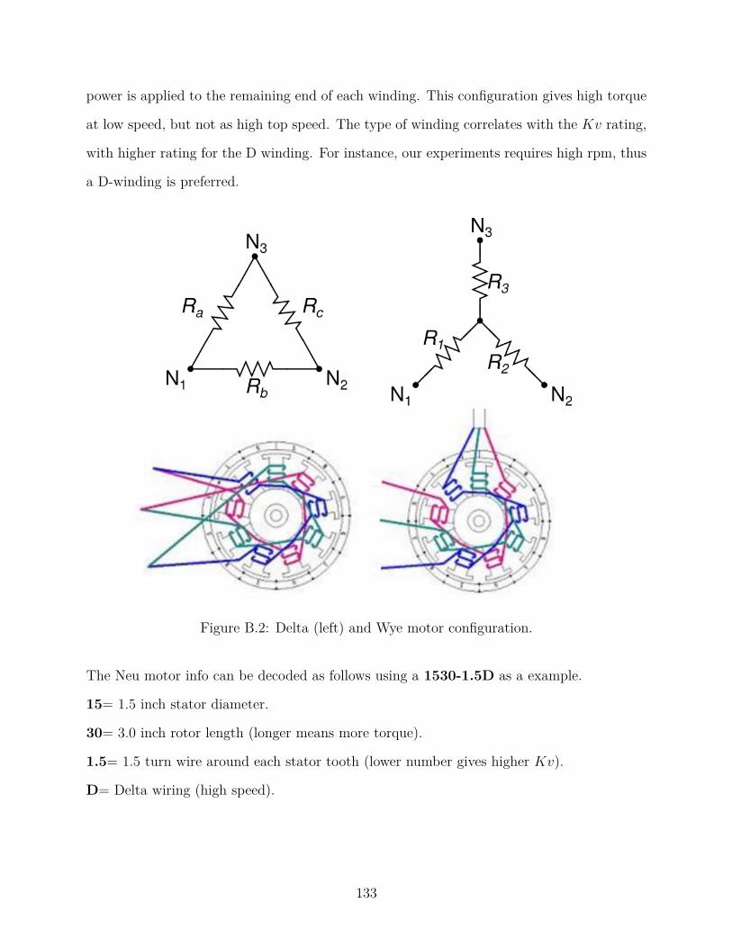
power is applied to the remaining end of each winding. This configuration gives high torque
at low speed, but not as high top speed. The type of winding correlates with the Kv rating,
with higher rating for the D winding. For instance, our experiments requires high rpm, thus
a D-winding is preferred.
Figure B.2: Delta (left) and Wye motor configuration.
The Neu motor info can be decoded as follows using a 1530-1.5D as a example.
15= 1.5 inch stator diameter.
30= 3.0 inch rotor length (longer means more torque).
1.5= 1.5 turn wire around each stator tooth (lower number gives higher Kv).
D= Delta wiring (high speed).
133
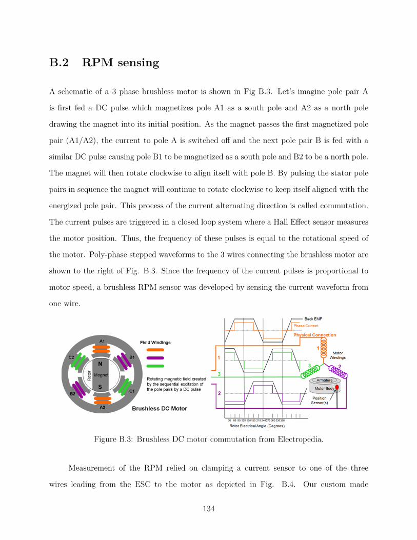
B.2 RPM sensing
A schematic of a 3 phase brushless motor is shown in Fig B.3. Let’s imagine pole pair A
is first fed a DC pulse which magnetizes pole A1 as a south pole and A2 as a north pole
drawing the magnet into its initial position. As the magnet passes the first magnetized pole
pair (A1/A2), the current to pole A is switched off and the next pole pair B is fed with a
similar DC pulse causing pole B1 to be magnetized as a south pole and B2 to be a north pole.
The magnet will then rotate clockwise to align itself with pole B. By pulsing the stator pole
pairs in sequence the magnet will continue to rotate clockwise to keep itself aligned with the
energized pole pair. This process of the current alternating direction is called commutation.
The current pulses are triggered in a closed loop system where a Hall Effect sensor measures
the motor position. Thus, the frequency of these pulses is equal to the rotational speed of
the motor. Poly-phase stepped waveforms to the 3 wires connecting the brushless motor are
shown to the right of Fig. B.3. Since the frequency of the current pulses is proportional to
motor speed, a brushless RPM sensor was developed by sensing the current waveform from
one wire.
Figure B.3: Brushless DC motor commutation from Electropedia.
Measurement of the RPM relied on clamping a current sensor to one of the three
wires leading from the ESC to the motor as depicted in Fig. B.4. Our custom made
134
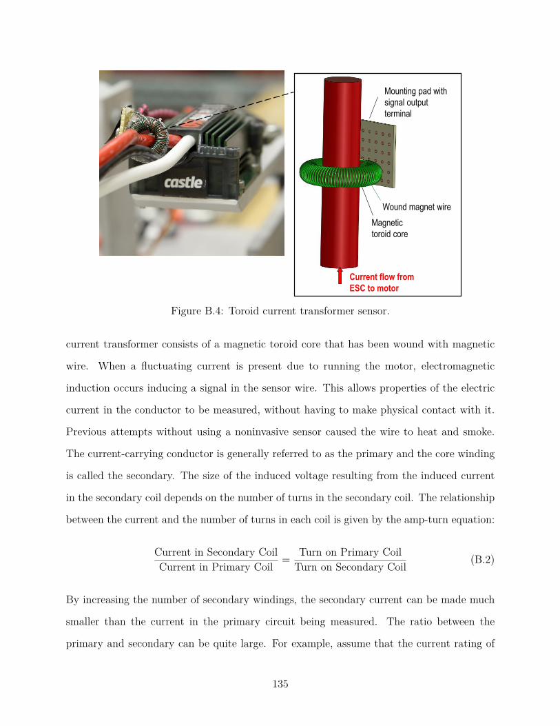
Current flow from
ESC to motor
Magnetic
toroid core
Wound magnet wire
Mounting pad with
signal output
terminal
Figure B.4: Toroid current transformer sensor.
current transformer consists of a magnetic toroid core that has been wound with magnetic
wire. When a fluctuating current is present due to running the motor, electromagnetic
induction occurs inducing a signal in the sensor wire. This allows properties of the electric
current in the conductor to be measured, without having to make physical contact with it.
Previous attempts without using a noninvasive sensor caused the wire to heat and smoke.
The current-carrying conductor is generally referred to as the primary and the core winding
is called the secondary. The size of the induced voltage resulting from the induced current
in the secondary coil depends on the number of turns in the secondary coil. The relationship
between the current and the number of turns in each coil is given by the amp-turn equation:
Current in Secondary CoilCurrent in Primary Coil = Turn on Primary Coil
Turn on Secondary Coil (B.2)
By increasing the number of secondary windings, the secondary current can be made much
smaller than the current in the primary circuit being measured. The ratio between the
primary and secondary can be quite large. For example, assume that the current rating of
135
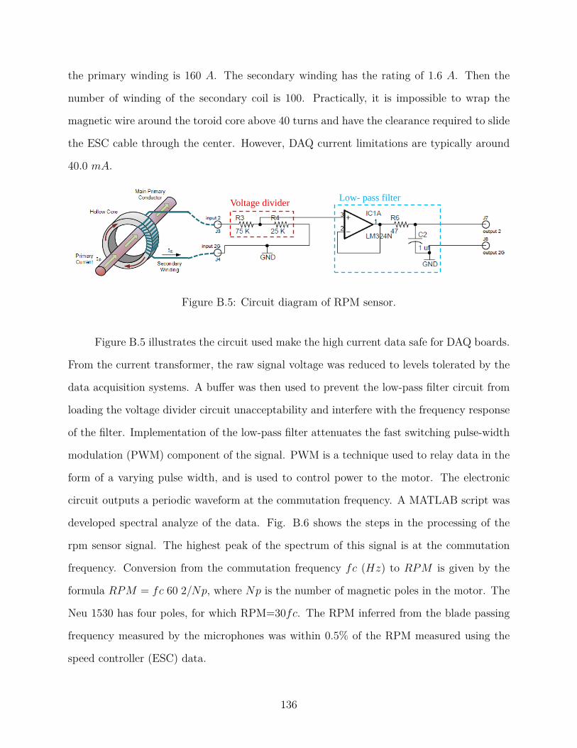
the primary winding is 160 A. The secondary winding has the rating of 1.6 A. Then the
number of winding of the secondary coil is 100. Practically, it is impossible to wrap the
magnetic wire around the toroid core above 40 turns and have the clearance required to slide
the ESC cable through the center. However, DAQ current limitations are typically around
40.0 mA.
Voltage dividerLow- pass filter
Figure B.5: Circuit diagram of RPM sensor.
Figure B.5 illustrates the circuit used make the high current data safe for DAQ boards.
From the current transformer, the raw signal voltage was reduced to levels tolerated by the
data acquisition systems. A buffer was then used to prevent the low-pass filter circuit from
loading the voltage divider circuit unacceptability and interfere with the frequency response
of the filter. Implementation of the low-pass filter attenuates the fast switching pulse-width
modulation (PWM) component of the signal. PWM is a technique used to relay data in the
form of a varying pulse width, and is used to control power to the motor. The electronic
circuit outputs a periodic waveform at the commutation frequency. A MATLAB script was
developed spectral analyze of the data. Fig. B.6 shows the steps in the processing of the
rpm sensor signal. The highest peak of the spectrum of this signal is at the commutation
frequency. Conversion from the commutation frequency fc (Hz) to RPM is given by the
formula RPM = fc 60 2/Np, where Np is the number of magnetic poles in the motor. The
Neu 1530 has four poles, for which RPM=30fc. The RPM inferred from the blade passing
frequency measured by the microphones was within 0.5% of the RPM measured using the
speed controller (ESC) data.
136
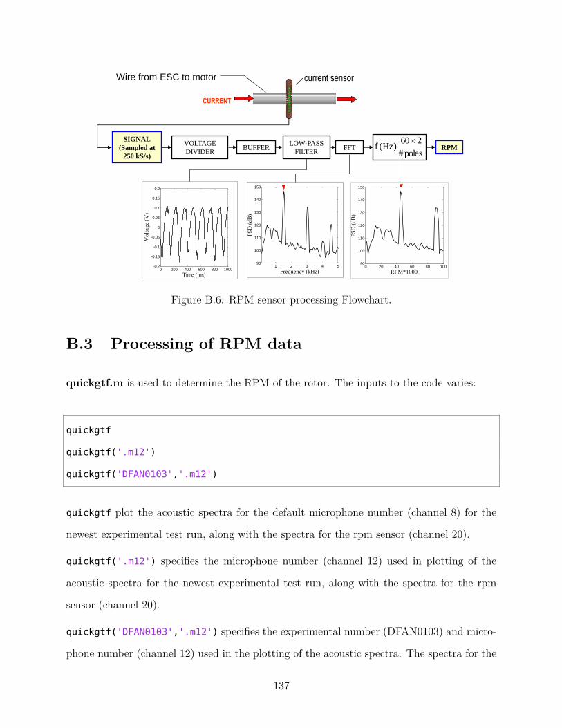
1 2 3 4 590
100
110
120
130
140
150
PS
D (
dB
)
Frequency (kHz)
SIGNAL
(Sampled at
250 kS/s)
VOLTAGE
DIVIDERBUFFER
LOW-PASS
FILTERFFT
poles#
260)Hz(f
RPM
0 200 400 600 800 1000-0.2
-0.15
-0.1
-0.05
0
0.05
0.1
0.15
0.2
Vo
ltag
e (
V)
Time (ms)
0 20 40 60 80 10090
100
110
120
130
140
150
PS
D (
dB
)
RPM*1000
current sensorWire from ESC to motor
CURRENT
Figure B.6: RPM sensor processing Flowchart.
B.3 Processing of RPM data
quickgtf.m is used to determine the RPM of the rotor. The inputs to the code varies:
quickgtf
quickgtf('.m12')
quickgtf('DFAN0103','.m12')
quickgtf plot the acoustic spectra for the default microphone number (channel 8) for the
newest experimental test run, along with the spectra for the rpm sensor (channel 20).
quickgtf('.m12') specifies the microphone number (channel 12) used in plotting of the
acoustic spectra for the newest experimental test run, along with the spectra for the rpm
sensor (channel 20).
quickgtf('DFAN0103','.m12') specifies the experimental number (DFAN0103) and micro-
phone number (channel 12) used in the plotting of the acoustic spectra. The spectra for the
137
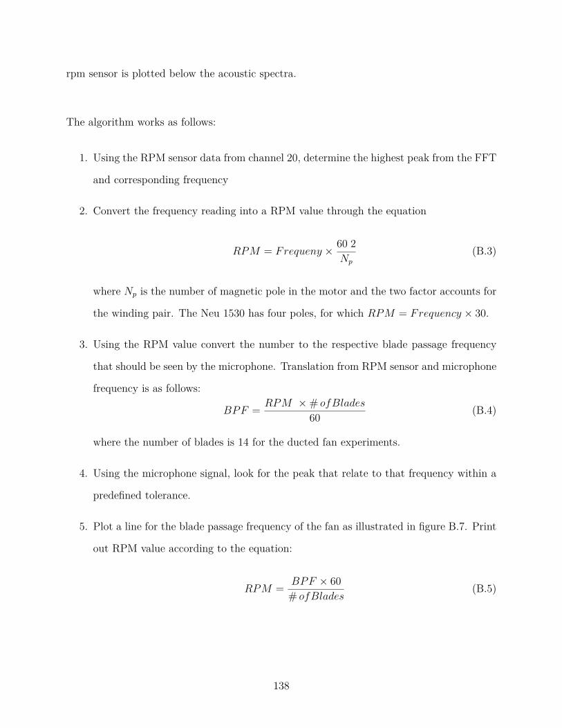
rpm sensor is plotted below the acoustic spectra.
The algorithm works as follows:
1. Using the RPM sensor data from channel 20, determine the highest peak from the FFT
and corresponding frequency
2. Convert the frequency reading into a RPM value through the equation
RPM = Frequeny × 60 2Np
(B.3)
where Np is the number of magnetic pole in the motor and the two factor accounts for
the winding pair. The Neu 1530 has four poles, for which RPM = Frequency × 30.
3. Using the RPM value convert the number to the respective blade passage frequency
that should be seen by the microphone. Translation from RPM sensor and microphone
frequency is as follows:
BPF = RPM ×# ofBlades
60 (B.4)
where the number of blades is 14 for the ducted fan experiments.
4. Using the microphone signal, look for the peak that relate to that frequency within a
predefined tolerance.
5. Plot a line for the blade passage frequency of the fan as illustrated in figure B.7. Print
out RPM value according to the equation:
RPM = BPF × 60# ofBlades
(B.5)
138
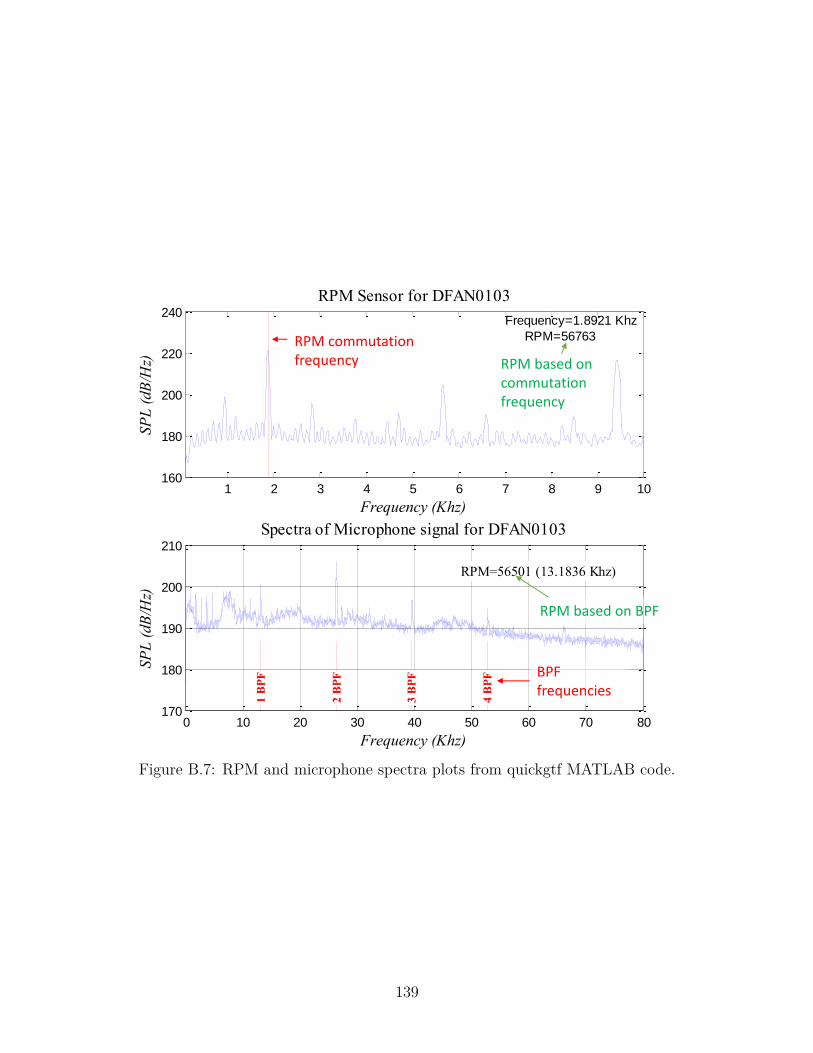
1 2 3 4 5 6 7 8 9 10160
180
200
220
240Frequency=1.8921 Khz
RPM=56763
SP
L (
dB
/Hz)
Frequency (Khz)
RPM Sensor for DFAN0103
0 10 20 30 40 50 60 70 80170
180
190
200
210
1 B
PF
2 B
PF
3 B
PF
4 B
PF
RPM=56501 (13.1836 Khz)
SP
L (
dB
/Hz)
Frequency (Khz)
Spectra of Microphone signal for DFAN0103
RPM commutation frequency
BPF frequencies
RPM based on commutation frequency
RPM based on BPF
Figure B.7: RPM and microphone spectra plots from quickgtf MATLAB code.
139