DISCLAIMER

This document was prepared as an account of work sponsored by the United States Government. While this document is believed to contain correct information, neither the United States Government nor any agency thereof, nor the Regents of the University of California, nor any of their employees, makes any warranty, express or implied, or assumes any legal responsibility for the accuracy, completeness, or usefulness of any information, apparatus, product, or process disclosed, or represents that its use would not. infringe privately owned rights. Reference herein to any specific commercial product, process, or service by its trade name, trademark, manufacturer, or otherwise, does not necessarily constitute or imply its endorsement, recommendation, or favoring by the United States Government or any agency thereof, or the Regents of the University of California. The views and opinions of authors expressed herein do not necessarily state or reflect those of the United States Government or any agency thereof or the Regents of the University of California.

{ )

. j(

l

u u u u -1

TRANSPORT AN ION OPTIC PROGRAM

LBL VERSION

Arthur C. Paul Lawrence Berkeley Laboratory

University of California -Berkeley, CA 94720

February 1975

TWO-WEEK LOAN' COPY

i This is a Library Circulating Copy . :_ .. f:: whi~h maybe botrbw~d_._·:_ior .. iwo~eeks. t ·•

.·-.:.- · ..

LBL-2697

. I.

0

Abstract ••

Introduction

u d 0 ~ 0 .i .;i 7 .....

-iii-

CONTENTS

Section 1 - Theory

Theory of Ion Optics

Matrix Method

Physical Significance of the Matrix Elements

Momentum and Energy Resolution

Phase Space Formalism on Optic Theory.

Definition of the Beam

Condition for a Waist

.•

9

.'-

Physical Significance of the Elements of the Beam •.

Betatron-Beam Transformations

Polygon Calculation and Beam Line Acceptance .•

Matrices and Vector Space

Numerical Nomenclature for Vector Space

Optimization of Variables

Variables and Vary Codes

Internal Constraint on Variables

Section 2 -- Standard Data Input, Option 0

TRANSPORT Data Deck Structure

Coordinate System and Sign Configurations

Data Input Format

Option 0, The Basic Data Deck

1. Beam Ellipsoid Input

2. Bending Magnet Pole Face Rotation

3. Drift Length

4. Bending Magnet

5. Quadrupole Magnet

6. Slit

7. Axis Shift

8. Misalignment

9. Repetition

10. Constraint

1-1

1-1

1-2

1-2

1-7

1-8

1-10

1-13

1-16

1-17

1-21

1-22

1-24

1-26

1-27

1-31

1-32

2-1

2-1

2-2

2-3

2-6

2-8

2-9

2-10

2-11

2-11

2-12

2-12

Z-14

2-15

11.

12.

13.

14.

15.

16.

17.

18.

19.

20.

21.

22.

23.

24.

25.

26.

27.

-iv-

Accelerator Energy Gain Section

Beam Correlation

Output Specification

Arbitrary Matrix

Unit Change. •

Parameter Input.

Second Order

Sextupole Magnet

Solenoid Magnet

Beam Rotation

Stray Field and Miscellaneous Input.

Particle Vectors •

Particle Separator

Plot Options • • •

Calculated Matrix.'

Space Charge

RF Buncher •

Section 3 - Modification of Data

Options

Option 1 Data Input.

Option 2 Data Input.

Data Array and Names •.

Option 3 Data Input.

Option 4

Option 5

Section 4 - Interactive Transports

Teletype Input Options

ABORT

ALINE

BEAM (TRAN3) or B

CANCEL (TRAN3) or C

FIN

FORCE (TRAN4)

FORCE, I, X.

GO . . . . . LABLE (TRAN4) or L

2-16

2-17

2-17

2-19

2-20

2-22

2-25

2-25

2-26

2-27

2-28

2-30

2-32

2-33

2-34

2-38

2-39

3-1

3-1

3-2

3-3

3-8

3-14

3-18

4-1

4-1

4-1

4-1

4-1

4-2

4-2

4-2

4-2

4-2

# ,.

•.

u u d 0 ,;:1 0 •' ~ s 0 • "' l

-v-

MATRIX or MA

MDATA (TRAN3) or M

NAME or NA

NCASE

OUTPT

PDATA or PD

POLYG and POLYG, MATRIX .. PRINT, LOC, LIST. (TRAN3)

PULL

RAY (TRAN3) orR

RECAL or RE

RESPN (TRAN4)

SAVE or SA • . SCALE (TRAN3) or SC

SEGMT (TRAN3), SEGMENTATION or SE

SNAPB (TRAN3) or SB

SNAPB (TRAN3) or SD

SOLVE or I

VARMIT INTERUPT

START

TABLE (TRAN4) or TA

TITLE or TI

TIME . TLOC (TRAN4).

VECT

Section 5 -- Running at Lawrence Berkeley Laboratory

Availability of Berkeiey Transport Code

LBL Transports

Loading at LBL

Setting Field Length

Setting Output Line Limit.

Starting a Teletype or Vista Job

Standard TRANSPORT Output

Example 1 - Optimization of Simple Quadrupole Doublet.

Example 2 - 130 MeV/c Muon Channel

Example 3 - ESCAR Ring • • • . •

Example 4 - K- Beam Line with n Contamination.

Example 5 - Astron Injection Trombone

Example 6 - Evaluation of Magnet Misalignments

Example 7 - Option 3 Chi-Square Search

Example 8 - LEP Channel Histograms • •

Example 9 - Pep, Long Beam Line Continued in Several Sequential Cases.

References .................................

4-3

4-4

4-4

4-4

4-5

4-5

4-5

4-5

4-5

4-5

4-6

4-7

4-7

4-7

4-8

4-9

4-9

4-9

4-10

4-10

4-11

4-11

4-11

4-11

4-11

5-l

S-1

S-1

5-2

S-2

5-7

5-11

5-15

5-15

5-15

5-16

5-16

5-17

5-17

5-19

5-19

6-1

•'

uuuu~·.~

1-1

ABSTRACT

TRANSPORT is a computer code for calculating properties of charged particle beam

transport systems using the matrix method in a six-dimensional phase space. At Berkeley

we have a version of TRANSPORT translated into FORTRAN by the author from the original

BALGOL SLAG TRANSPORT. We have included many addititional elements, options and pro­

cedures which are explained here. along with a standard TRANSPORT user's manual. Some of

the important additions are polygon transformation, ray, tracing, particle separator, space

charge, output plotting, interactive on-line calculations, ·and flexible data manipulation proce­

dures.

INTRODUCTION

TRANSPORT .is a computer code for the evaluation of charged particle beam transport 1

systems. It evaluates a given beam line by calculating the six-dimensional transformation

matrix of the line in terms of its physical parameters, such as magnetic field strengths and

magnet spacings. This transformation matrix may be used to transform given particle vec­

tors along the beam line, transform a six-dimensional phase space ellipsoid along the beam

line representing the particle bunch from an accelerator, or transform the various apertures

encountered along the beam line to a specified location so as to evaluate the beam line accep­

tance and solid angle. TRANSPORT will also produce useful summary tables and graphs of

the beam, vectors, acceptance polygons and phase space ellipses when directed to do so.

Some of these calculations may be carried out to. second order.

Often a user does not know all the parameters of his system, but knows apriori the re­

sults he desires. He may represent these results in the form of constraints on the system

and designate that TRANSPORT is at the liberty to vary certain specified parameters in order

to satisfy these constraints through first order. Constraints may be placed on the accumulated

length, the accumulated transformation matrix elements, the beam phase space projections and

tilts, the beam centroid (analogous to constraining a vector) or any given combination of the

constraints.

The variables at a users command are the beam phase space dimensions, drift lengths,

bending magnet fields, indices and angles of entry and exit, quadrupole lengths and fields,

solenoid length and fields, phase plane rotations, and magnet misalignments and axis shifts.

Combinations of these may be varied to produce the specified results.

The six dimensional beam phase space ellipsoid represents the particle bunch eminating

from an accelerator. The particle distribution from a secondary production target can better

be analyzed by considering the beam line phase space acceptance. TRANSPORT will calculate

this acceptance and additionally can transform up to 40 particle vectors along the beam line.

These vectors can be used to represent beams of several momenta (small dp/p) or beams of

several particles of the same momenta such as tr- and K- beams to be separated by particle

separators. TRANSPORT will also calculated the acceptance area (solid angle) as a function of

momentum so that the expected first order flux can readily be estimated, see Option 5 and

polygon calculation.

1-2

Finally, TRANSPORT will allow a user to cycle any parameter or any set of up to four

parameters over a given grid or randomly and evaluates the rms deviation to the specified con­

straints (Option 3). The result is the functional dependence of the constraints on the selected

variables and is very useful in solving problems sensitive to starting conditions.

Section 1 - Theory

THEORY OF ION OPTICS

We will consider a beam transport system to be made up of a series of magnets (dipole,

quadrupole, and sextuple), drift spaces,' and such special elements as velocity separators, etc.,

through which a charged particle beam progresses. A particle source at z = 0, such as a cyclo­

tron, emits individual particles along some limited range of directions. The extreme trajec­

tories determine the beam envelope propagating in the z direction. This envelope is ben~ and

displaced through physical space by the interaction of t4e particles with the fields of the magnets.

To ease the problem of drawing the particle's trajectories, it is customary to straighten out the

z axis, masking all deflections of the physical reference axis. This straightened z axis is re­

ferred to as the optic axis or paraxial ray;· and all particle positions and directions are given as

displacements from this axis and its direction in physical space. A cut in the vertical plane

(y axis) from the optic axis outward is drawn, by convention, above the optic axis. A cut in the

horizontal plane (x axis) from the optic axis outward is drawn below the optic axis, as shown in

Fig. 1. An individual ray in the horizontal plane (dotted line in Fig 1) which passes through the

optic axis (x = 0) is represented by a change in sign (reflection) at the point of zero passage. A

waist is said to occur at the point of minimum beam dimension in either plane.

Th optic axis of a beam of particles is actually the trajectory of a particle of the desired ' energy (dE = 0) leaving the source with zero displacement (x andy) and zero emergence (x and

' y ) . The energy of the optic axis is unique, particles leaving the source at z = 0 with x = y = ' ' x = y = 0, but with energy different from that of the optic axis will be displaced from it due to

' ' dispersion effects in bending magnets. Off energy particles with nonzero x, y, x , and y will

come to a focus longitudinally displaced from the focus for the paraxial energy due to the chro­

matic abberations in the various focusing elements.

Matrix Method

TRANSPORT uses a matrix formalism2 to represent a charged particle beam line made of

various magnetic elements. This formalism assumes that the output vectors of an arbitrary ,

magnetic configuration can be expanded as a power aeries in the initial vector elements. If we

' ' consider a six-dimensional differential vector space x, x , y, y , s, o whose quantities are a mea-

sure of the displacements from the paraxial trajectory, then

' ' 2 ' R11x0~ R12x0 +Ri3yO+R14YO + R15 8 0+ R16°0~ R17x0 +R18x0x0 + X=

' ' 2 R21xo+R22xo +R23Yo+R24Yo + R25 8 o+R26 6o+ R27xO +R2sxoxo + • • • X

' ' 2 ' R31x0+R32"0 +R33Yo+R34Y0 +R35 8 0+R36°0+R37x0 +R38x0x0 + y

' ' 2 ' R41x0+ R42x0 +R43Y0+ R44Y0 + R45 8 0+ R46 °0+ R4~0 +R48x0x0 + y

8 ' ' 2 ' R51xo+R52xo +R53Yo+R54Yo + Rssso+R56 6o+ R57xO +Rssxoxo +

Bo

-,

1-3

N y

s

y Vertical

x Horizontal

y

tic axis

Beam envelope

Individual particle

z

XBL747-3695

Fig. 1. Typical external beam system and its ideal representation.

1-4

I

where xo· xo • y 0' y 0 • so· and 00 are the initial small deviations from the paraxial trajectory

and the expansion coefficients R .. are functions of the magnetic field parameters such as, cur­lJ

rent in the magnets, distance between the magnets, etc. I

In a first order theory, we assume x0

, x 0 , y, y0

, s0

, and o0

to be small so the all I

terms RNM and higher may be neglected for M greater than 6. In the expansions of x, x , y, I

y and s, the initial coordinates are considered small when x 0 , y0

, s0

are much less than the I I

radius of curvature of the bending magnets and when x , y expressed in radians and o = dp /p

are much less than unity. Then, the trajectory expansions may be written as:

V=R1

V1

=

11 R12 R13 R14 R15 R16

R21 R22 R23 R24 R25 R26

R31 R32 R33 R34 R3 5 R36

R41 R42 R43 R44 R45 R46

R51 R52 R53 R54 R55 R56

R61 R62 R63 R64 R65 R66

X

I

X

y

y

s

where V 1

is a particle vector and R1

the first order transformation matrix.

When higher order terms are to be included in the expansions, the matrix formalism can

still be applied by linearizing the higher order terms with the attendant increase in the dimension­

ality of the vector space. The theory has been extended by K. L. Brown3 and by M. F. Tautz 4

to include third order terms in the transformation matrix. In first order, TRANSPORT works I I

in a six-dimensional vector space x, x , y, y , s, o. In second order, the vector space is 42-

dimensional (although this could be reduced to 27 dimensions by use of the obvious symmetries)

such that if V is the first order vector, then the second order vector is V + V ** 2, e. g.,

I I 2 I I I r2 1 I I I

X,X ,y,y,s,o,x,xx,xy,xy,xs,xo,xx,x ,X y,x y ,X S, X o,yx

The second order transformation matrix construction is:

[ - (Ri) I aberrations

R I - -1 -0 I (2nd order ]

I matrtx elements)

where (R1

) is the 6 X 6 first order matrix and the second order matrix elements are the

square of the first order elements, e.g.,

2 X

u u u ;··· 0

1-5

So

{

J = 1, 6

R(6J + K, 6N + M):: R (J,N) R (K,M) for ~: ;:~ ..

M:: 1, 6

The aberrations R( N, M) are related to the second order aberration coefficients of Ref.

3, T(ijk), as follows

R(N, 6J + K)

R(N, 6K + J)

1/Z[T(N, J, K) + T(N, K,J))

R(N, 6J + K).

For a moment consider the general 6 X 6 matrix to be de-coupled into a horizontal bend

matrix and a vertical nonbend plane matrix. The de-composition is

[:. ]= [::: ::: :::] [ ::· J dp/p 0 0 1 dp/p

}~ the horizontal plane and

in the vertical plane.

The transformation representing a field free region in which there are no magnetic

forces is

This matrix translates the vector

L inches downstream along the z axis.

X

I

X

The matrix representing a bending magnet with a nonuniform field characterized by a field

index n is

r 112

l cos( 1-n) a

1/2 A___ (1-n) . ( 1 · )1/2 _li - - R s1n -n a

0 .

in the bending plane and by

1-6

R(1-n)1/ 2sin( 1-n)1/ 2 a

cos(1-n) 1/2 a

0

1 ~[ 1-cos(1-n)1/2 a] l

-1/2 1/2 (1-n) sin(1-n) a

1

[

cos n1/ 2 a

Ay = 1/2 n . 2 --a· smn1/. a

-1/2 1/2 .] Rn sin n a

1/2 cos n a

in· the nonbendi ng plane. Here n = - ( dB/B)/(dR/R), a is the. angle of bend ·and R is the

radius of curvature of the particle in the g.iven field.

Say the bending is in the horizontal plane; then a horizontal component to the field exists,

should the particles enter or exit the magnet at an angle of other than 90 degrees. This hor­

izontal component, B , produces a vertical focusing force. Also, the path length in the magnet X

is changed depending on which side • of the optic axis the particles are located, producing a hor-

izontal focusing.

These forces are characterized by the following focusing matrices for non-normal entry

and exit.

Here 131

and 132

are the angles between the normal to the pole face and the direction of propaga­

tion.

where

A quadrupole magnet has matrix elements given by

[cos KL Ac =

- K sinKL

[cosh KL Ad =

K sinh KL

k sinKL]

cosKL

1 K sinh KL J cosh KL

dB da

r

u u J / -1-7

Bp is the magnetic rigidity of the particles, dB/da the gradient, and L the length of the lens.

The Ac matrix represents the convergent plane in that a beam entering the magnet parallel to

the optic axis leaves the lens converging to a focus some distance beyond the lens exit. Ad rep­

resents the other plane, where this parallel beam leaves the lens diverging from the optic axis.

Focusing in both planes can be achieved by alternating the polarity of several lenses.

A divergent second lens does not destroy the focusing produced by the first lens. This is

so because the magnetic forces are proportional to the displacement from the optic axis, so that

divergent force is less than the convergent force. The opposite is true in the plane where the

second lens is convergent. Here the beam displacement has increased by the defocusing of the

first lens so that the converging force of the second lens is even stronger.

Physical Significance of the Matrix Elements

A focus is a location where the displacement from the optic axis is independent of the angle

of emergence from the source. Since

' This requires R12

= 0 for an arbitrary x0

• A vertical focus is characterized by R34

= 0. In first

order ray trace theory, the equations are linear, so we have the situation in which if we double

the off-axis distance of the particles at the input, we double their value at the output provided we

are .at a focus where R12

= 0

Then the magnification is defined as x/x0

and is therefore independent of the value of x0

or y 0 ,

so that;

Horizontal Magnification - x /x -- image input -

Vertical Magnification - y /y -- image input -

It is important to stress that the focus condition and magnification at the image are in terms

of the matrix elements representing the physical region extending from the input to the image.

The fact that the magnification in the horizontal plane is R11

is a result of the definition of a focus,

that is, a point where the displacement is independent of the angle so that R12

= 0.

If we assume we have a mono-energetic extended source of particles, we will have an ex­

tended image at the focus as a result of the finite magnification of the system. The image size

will be x. = R 11 x where x is the size of the source. If we have a momentum spread dp/p the 1 s s

image size will be increased to xi= R11

xs + R16

dp/p. Hence the matrix element R 16 gives the

contribution to the horizontal displacement by the momentum spread of the system, i.e., it is a

measure of the dispersion.

R16 dp/p.

1-8

Similar physical significance can be attributed to all elements of the transformation matrix.

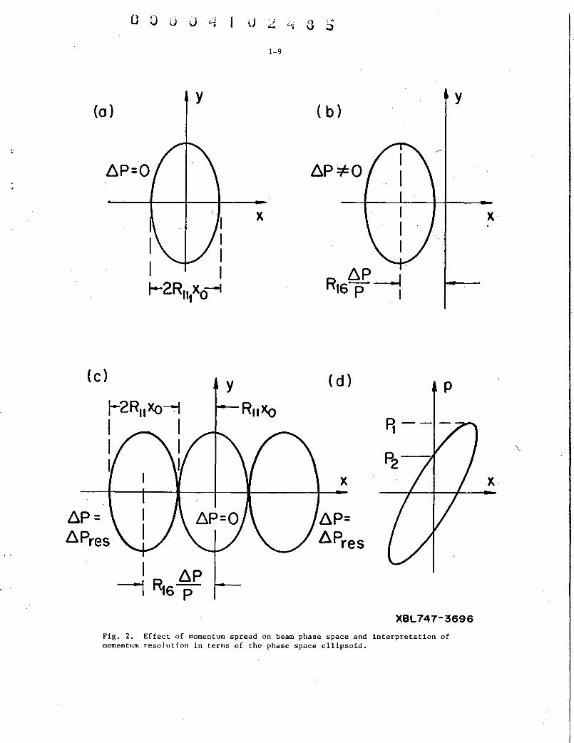
Momentum and Energy Resolution

The energy resolution of a system is defined as the energy spread dE in a beam of energy

E such that particles whose energy is outside the range E ± dE/2 will not be transmitted and par­

ticles whose energy is within this range will be transmitted. Consider the beam spot for a finite

size source of particles with dE = 0, Fig. 2a. A group of particles with dE larger energy than

this beam will be horizontally displaced due to the dispersion of the system introduced by bending

magnets, (Fig. 2b). The amount of displacement is R16

dp/p. If a slit system of 2R11

x0

width

is located here, the maximum energy spread that can get through the system is determined by the

condition that R16

dp/p is e51ual to 2R11

x0

. Particles with dp/p larger than this value do not get

through the system. 2 R11

x0

is the full beam size for dp/p = 0.

The full energy spread in the beam is

AE = res

However, a beam may have a non-uniform particle distribution with momentum so that a more

meaningful definition of the resolution would be the full width at 1-/2 maximum transmission.

and the full energy spread in the beam for 100"/0 transmission of the central momentum (dp/p = 0)

and less than 1/2 maximum transmission of particles with dp/p ~ (dp/p)FWHM is given by

The resolution is a property of a given magnet system. It is independent of the particle

input vector or phase space ellipse and is determined solely by the matrix elements of the trans­

formation. For example, if a 2% energy spread is inherent in a beam incident upon a system

that has a resolution of 0.5"/o, then a beam reaches the target for which there has been 100%

transmission of particles with dE= 0, 50% or more transmission of particles with dE~ 0.5"/o, and

very little transmission of particles with dE <l: 1"/o. If one chooses to narrow the momentum de­

fining slits in the system, he does not improve the resolution of the system but he may reduce

somewhat the energy spread of the beam reaching the target at the expense of particle intensity

for particles with dE= 0. He may not, however, reduce the energy spread indefinitely by a suf­

ficient reduction in slit width. This results from the presence of particles of different energies

with various emergencies (angle to the z axis) so that even for an infinitesimally narrow slit a

finite energy width will be transmitted. Alternatively this may be seen by projecting the phase

o i, ~~ u·· ~.~ ,. il o v._ u.:::i..~u~

1-9

(a) (b) y y

X

(c) y (d) p

X

8P=

XBL747-3696

Fig. 2. Effect of momentum spread on beam phase space and interpretation of momentum resolution in terms of the phase space ellipsoid.

X

1-10

ellipse of the particles onto the p-x plane (Fig. 2d). For x- 0 we have a reduction in trans­

mitted momentum spread p from p1

to some finite irreducible minimum value p 2 .

Phase Space Formalism of Ion Optic Theory

Now, with a general understanding of the matrix representation of magnetic fields we can

consider the phase space formulation of beams of particles. This formalism is important since I

the conservation of phase area implies a relation between displacement and emergence, A ;:. xx •

A single particle represented by a vector can be traced through the system by matrix multiplica­

tion; however in nature, we are not confronted with single particles, but rather groups of par­

ticles comprising a beam that ·we wish to transform from a source to some target restricted by

specific constraints. These particles comprise a beam. If n coordinates are required to spec­

ify a given particle, then a group of particles will occupy a certain volume in n-space. If these

particles comprise an internal beam of an accelerator they will be executing betatron oscillations

which are independent in the axial and radial planes to first approximation. The radial differen­

tial equation is

so that

X

The axial differential equation is

so that

2 + w (1-n) x = 0

x sin (1-n) i/2 wt. m

d2y + 2

dt2 w ny = 0

. 1/2 t y=yMstnn w.

The transverse momentum associated with these motions are given by px = M ddxt and p - M ~ y - dt

p = Mni/2 wy cos n 1/ 2 wt. ,Y m

The amplitude of the displacement in the radial direction is x while the amplitude of the corre­

sponding momentum is M(l-n) 1/2 wx . Time can be eliminate: by using the properties of the tri­m

gonometric functions.

. 1/2 2 1/2 2 [stn(1-n) wt) +[cos(i-n) wt] 1.

This is the equation of an ellipse independent of time. Similarly in the vertical plane we have

u u u . )

,.;..

1-11

d 6

+ ( Sr )2

• Mn <Jim

If we have many particles distributed in time with the same oscillation amplitudes xm or ym'

they will comprise an ellipse in the corresponding phase space. If we focus our attention on

one single particle it will rotate around on its ellipse as time passes, confined indefinitely to

its own ellipse provided phase space is conserved, i.e., the momentum (energy) is constant,

etc., Fig. 3b.

In an accelerator we have present particles of many oscillation amplitudes ranging from

zero up to some maximum value xm. Considering the sum of all particles in the horizontal

plane we have a two dimensional ellipsoid. Any one particle belongs to a given ellipse within

this area phase ellipse, and rotates about its own ellipse with time. The particles simultan­

eously belong to a phase ellipse in the axial direction. In general, the particles can be de­

scribed by six coordinates, and hence will lie on a six-dimensional elliptical surface within a

limiting six-dimensional ellipsoid characterizing the particle distribution. The six coordinates

are the particle's axial and radial displacement and momentum, and the longitudinal displace­

ment and mo:rt:lentum.

The conservation of phase space guarantees that the volume or area of the ellipse re­

mains constant during the motion while the linearity of the first order theory ensures that the

distribution remains. ellipsoidal. Consequently, the motion of a "beam" through magnetic sys­

tems can be described by the transformation of the particle's phase ellipse. This motion ro­

tates and stretches the phase ellipse subject to the condition that its area or volume remains

constant. The actual extent of the particles observed· in the physical world is the projection of

this ellipse onto the coordinate axis.

In calculating the particle distribution as it progresses through space after extraction

from an accelerator, it is eonvenient to change the units of the phase ellipsoid. Note that in ac­

cordance to the first order theory the angles of emergence of the beam are small so that

p X z

pz is the momentum of the particle in the z direction, the direction of motion. The volume

of phase space of an upright ellipse whose semi-axis coincides with the coordinate system is

And 'the area projection onto one pair of coordinate axes is

I

A "" 1TXX X

A "" 1T'fY y A "" 1rzpz z

1-12

Px

1 . ~

_&=m(1-n) wxM

X

(a) {b)

9

v'CT22 --(1 - 2 )1/2 r;:---

r12 v CT22

{ c)

Px

/ '\. I

' I

I \ I \ / .......

~fl11 I I 2 112 l..fo11 (1-r12)

XBL747- 3697

X

Fig.3. a,b) Simple harmonic oscillation phase plane motion typical for simple magnets encountered in beam lines.

c) Interpretation of ellipse projections and TRANSPORT beam correlations r 12 in the horizontal phase plane.

-:

1-13

The constant ·of proportionality is the momentum p which is constant as long as the energy is z

not changed. The equation of the phase ellipse in the principal coordinate system is

( ' 2 ( I ) 2 ( )2 ( I 2 x:) + :01 + f;; + y:l ) + ••• =1.

The coefficients 1/x0

2, etc., ~haracterize the particle' s distribution. This equation can be

written in matrix form as

1 0 0 .......... "l 2 X

xo I I 1 I

(x,x ,y,y, ••• ) 0 -,-2 0 X =1.

xo 1 0 0 -,-2 y·

Yo 1 -,-2 y

Yo _)

Thereciprocal form of the coefficients (1/x02) suggest that we define a matrix 0"-i as

then

-1 ()"

()" =

0

0

0

1 -2 Yo

2 Yo

1 -~-2

Yo

'2 Yo

The matrix u is called the "beam matrix", or simply the beam.

Definition of the Beam

We have shown that the particle distribution is an n-dimensional ellipsoid and we have

written this as 2 I 2 2

a11 X t a22 X t a33 y t • • • • = 1.

1-14

This is the equation in the principal coordinate system. If the coordinates are rotated, we have

the case shown in Fig. 3c. Here the equation for the ellipse will involve various off-diagonal I

terms, such as xx . For example, in two dimensions we would have

I I 2 - a

21 X X t a 22 X = 1.

The cross terms give the measure of the rotation of the ellipse.

In n dimensions, the equation of a tilted ellipse is

n n

2I j

a .. x. x. = 1. lJ 1 J

We can define the matrix of the coefficients a .. as describing the ellipsoid and consequently, lJ

defining the particle distribution. This beam matrix is written as

or

-1 C1

-1 C1 a ..

lJ

A single particle described by a vector V transforms through a magnetic system described by a

matrix R as

The ellipsoid character of these particles can be written as

as can be seen by the. following:

I

(x,x , 6) [

a

a1

2

1

1

a12 a13]

a22 a23

a31 a32 a33

[ :·] = 1

and if the cross terms a .. (i ~ j) vanish (the ellipse is then upright) and we have lJ

u u 0 ('•

0

1-15

The transformation of the ellipsoid through a magnetic system characterized by the transforma­

tion matrix R then gives the transformation of the particle distribution. Noting that R - 1 R = 1,

then the ellipsoid VT a - 1 V = 1 can be written:

VT(R- 1R)T a- 1(R- 1R) V = 1

(VTRT) RT-1 a-1 R-1(RV) = 1

(RV)T (RaRT)-i (RV) = 1.

Where we have used the fact that the reciprocation of a matrix product requires reversal of the

order of factors:

AB=C

B-i A-i ABC-i = B-i A-i C C- 1

B-1 A-1 = C-1

(AB)-1 = C-1

and the fact that taking the transpose of the product of two matrices is obtained by taking the

product of the transposed matrices in reverse order

Therefore

Defining the vector after transformation as v1

= RV, we obtain

where

-1 T -1 a1

= (RaR ) •

That is to say, the ellipsoid after the transformation is a relation between the transposed particle

vectors which comprise the distribution and the beam a 1

characterizing the coefficients of the

phase space ellipsoid.

a 1

has been defined from above as

In other words, given the beam a at the entrance of the magnetic system and the transformation

matrix of the system, the "beam" a1

at the output can be calculated from the above expression.

The first order beam is in general defined as:

1-16

Now consider the distinction between a matrix representing a waist condition and a matrix

representing a focus condition. A focus matrix is defined as a transformation matrix with R 12= 0,

so that x = R11

x0

. A transformation matrix representing a waist transforms a beam so that

cr12 = cr21

= 0. The transformation of an upright phase ellipse by a matrix representing a focus

is given by

C" R 21

o ) (x0 2 R22 o o.,IC''

xo I o R21) R22

(Rtf 0 ) (Rtf x0 2 R21 xa')

R21 R22 o R ,2 22 xo

For a finite x 0 we have cr 1

non-diagonal, hence by definition not representing a waist. In order

to have a waist we would need cr 12

= cr21

= 0, i.e.,

For a matrix with non-zero R 12, we would have

CT = 1

The general requirement for a waist is

u u u J ~ '' . u ~ 'i (J 9

1-17

2 '2 For a non-zero R11

, R22

and a finite x0

and x0

, a sufficient and necessary require-

menton the transformation matrix in order to satia!y the condition that a waist be present is

Note. that !or a point source (x0

= 0) the focus matrix would be identical to a matrix repre­

senting a waist transformation. For a finite source size the two transformations are distinct.

Physical Significance of the Elements of the Beam

Physical significance can be given to the elements of the beam as they have been defined

here. Consider an arbitrary ellipse defined by the beam

We have alr.eady shown that this can be written as

This is the equation of an ellipse rotated lro·m the coordinate axis. I! a 1 z is zero, the ellipse

is upright; it a12 is non-zero, then it is a measure of the tilt of the ellipse.

To picture the ellipse we must know the values of its intersection points with the coordi­

nate axis and the values of the intersection points with its projection rectangle, Fig. 3c. To

find the intersection points with the coordinate axis, we take x = 0 so that

Defining

as the correlation coefficient, we obtain

I

X _,.......- Z 1/Z =""azzU-ru> .

t I

This is the point of intersection of the ellipse with the x axis. I! we take x = 0, we find

2 X 0"22 :

or

: ::·.' ·.,

This is the point of intersection with the x axis.

To find the intersectio~ points .of the. e~~ipse vr.:ith. its projection .. rectangle we note that

the slope is. a maximum, ,or minimum. Thus,. differentiating the equation of .the elli,Pse

I dx I

dx (2x <T 11

At the tangent point we .have I

dx/dx = 0 so that ' '

X -1

X

<-· .. .·'").

~12. ,] ,, .

a22 .···

i. ,.

Therefore :X 1:: a 1.2 x1 :·~ "\\Then 'this 1s substituted ti1to· the ellipse equation we obtain a22 ~

I

x = .Ja22

So the coordinate of the intersection point is

I

Similarly, at the other tangentpointwehave dx/dx = 0 so that

Therefore,

I

X

X _; ; ....

0"12 ' x = -- x, when this is substituted. into the ,,ellipse equation we obtain

0"11

. :.

:• ... !.

The physically measurable coordinate projections are x ~ and x1= .Ja22 •

u u u u .....

1-19

These are the square root of the diagonal beam matrix elements. Figure 3c shows the geometric

points of the phase ellipse in terms of the matrix elements. Program TRANSPORT prints as

output the following beam matrix:

~ ~ r21

~ r31 r32

.J (144 r 41 r 42 r43

~. r 51 r52 r53 r54

.fU66 r 61 r62 r63 r64 r65.

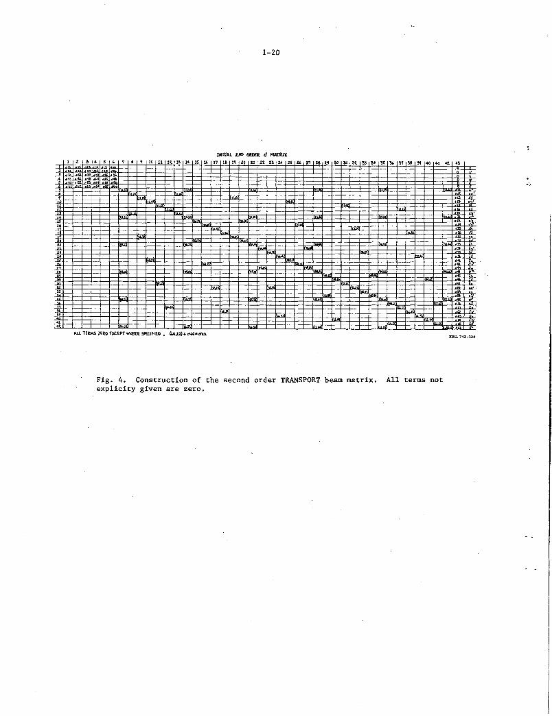
Since cr .. = cr ..• we have r .. = r... The second order beam matrix u is given in terms of the 1J J 1 1J J 1 '

initial first order u matrix elements as:

for { J:7,14,21,28,35,42 · K-7,14,21,28,35,42

Explicitly, the second order vector space is as follows:

Vector Vector element Vector Initial element Vector Initial number parameter value number parameter value

1 X 0 25 Y'X (141 2 x• 0 26 Y'X 0"42 3 y 0 27 Y'Y (143 4 Y' 0 28 Y'Y' 0"44 5 s 0 29 Y'S 0"45 6 0 0 30 Y' o 0"46

7 x2 0"11 31 sx 0" 51

8 XX' 0"12 32 sx' 0"52 9 XY (113 33 SY 0"53

10 XY' 0"14 34 SY1

0"54 11 XS

0" 15 35 ss 0"55 12 xo

0" 16 36 so 0"56

13 X'2 0"21 37 oX 0"61 14 x• u22 38 oX 0"62 15 X'Y IT23 39 oY 0"63 16 X'Y' 0"24 40 oY' 0"64 17 x•s 0"25 41 02 (165 18 X' o 0"26 42 0 0"66

19 YX 0"31 20 YX'. (T32 Where the u JK are the first order 6X6 21 YY (133 matrix elements. 22 YY' 0"34 23 YS 0"35 24 Yo 0"36

l z ~

~ @; ~f ,., :1: .43>

+ . I

..l

JS

" .J

: ... •

..1.

* ...l

...l ~~ ..... ··- ·-

1-20

lNITAL l.)f1> oeDER. d MA11UX 4 5 ' 7 • , lO 11 u. lS l4 lS u 17 l& 1, t z~ Ll 21 25 ,.. u 1.4 21 21 ~· 30 l>1 ·~ •• ~

?..-~ -H ... ..: ...

I

Fig. 4. Construction of the second order TRANSPORT beam matrix. explicity given are zero.

!S .... ., ;s ,. 40 ... 42. • •

'

•

... ~ u

XBL 7tl-3Z4

All terms not

0 0 u J ~ U '.i

"- -4

1-21

The u-matrix has by mathematical construction an elliptical boundary on any plane on

which it is projected. When second order calculations are performed the u-matrix takes on

the interpretation of a circumscribed ellipsoid containing the real nonlinear phase space. The

actual nonlinear transformations will be performed by TRANSPORT whereever a plot card

(24. ijkl.) is used to generate plots. In this calculation the second order accumulated matrix

(RC-matrix) is used to transform 36 boundary points on th~ initial projected phase space and

these are shown as points (.) on the plot. T.he circumscribed ellipsoid is also plotted by (x) and

may be considerably larger than the actual phase space due to the distortions introduced by the

nonlinearitie s.

Betatron- Beam Transformations

The betatron functions introduced by Courant and Snyder 5 have meanings completely

analogous to the elements of the u-matrix used by TRANSPORT. In a two-dimentional phase

space of area trE, the betatron function a, j3, and y are related to the u-matrix as

so that

CJ = E (13 -a\ -a 'Y}

(]22 yE

(]11 = .j3E

(]12 =-a E

where u12 = r 12 .Ju11

u 22 , r12

being the beam correlation coefficient and E is the phase area

divided by tr. Betatron functions can be introduced as input to TRANSPORT by proceeding

the beam card by a 21.0. card giving the radial and vertical phase areas Ex and Ey. These

areas can be calculated from the u-matrix as follows

j3y -2

1 a =

(]11 u22 = E2f3'V

(]12 (]21 = E2a2

so that

det u.

TRANSPORT will also allow constraints to be placed upon the betatron functions and will gen­

erate a table of the a, j3, y 1 s as described elsewhere in this report.

1-,22

Polygon Calculation and Beam Line Acceptance

The beam line transmission is determined by how well the acceptance of the beam line

is matched to the emittance of the particle source. TRANSPORT will calculate the enclosed

polygon in the horizontal and vertical phase space determined by the apertures encountered

along the beam line. Physically, only particles which are within this polygon will success­

fuily negotiate the apertures of the beam line and therefore be transmitted. If a target is in­

cluded in the data (24.1. Data Entry) the solid angle acceptance will also be calculated. Plots

of the beam acceptance showing the polygon, beam ellipsoid and particle vectors can also be

made.

Aperture information is processed at the beginning and end of each quadrupole, particle

separator, and sextupole and at the location of slits designated by a 6. or 16.4. and 16.5. data

card •. Aperture information may be specified for bending magnets, drift spaces and solenoids

by using the slit. options which designate apertures for succeeding beam elements possessing

length. When the .16.4.H. and 16.5N. aperture cards are used they will specify apertures for

all succeeding bending magnets. These apertures are transformed backwards in the phase

space under the assumption of decoupling of the phase planes. This restricts the aperture cal­

culation to beam lines which do not contain solenoids, misaligned quadrupoles or other elements

which mix the horizontal and vertical planes. Circular apertures are approximated by square

apertures in the pblygon calculation. In order to account for the reduction of the quadrupole

apertures by beam plumbing a fractional fillage can be specified by the 16. [16.X. data card

where X] is the length of the circumscribed square leg divided by the quadrupole diameter.

The polygon calculation is initiated by Option 5. The calculation begins at the location

of the 13.5. data card which specified the location where all apertures will be transformed.

This card may be placed anywhere along the beam line, though generally it is particularly

meaningfull when placed at the location of the particle source. The table of verticies of the

enclosed polygon, polygon area .and plot of the polygon and beam are printed at each location

where a 13.6. Data Card appears.

The vertices of the enclosed polygon are tagged as to which apertures intersect at that

vertex.

TAG= TYPE+ I/1000

e. g., a bending magnet (Type 4) which is the 62 element in the beam line (I value 62) has a tag

= 4.062. The I value for each type is printed at the beginning of each data calculation along

with the data set. Each vertex is also tagged with the name of the aperture which lies counter­

clockwise from the vertex as shown in Fig. 5. The vertices are also ordered counter clock­

wise.

The phase space coordinates of the vertex are also given and may be interpreted with

the aid of Fig. 5 for the Jth vertex. The solid angle acceptance for a finite target may be cal­

culated in addition to the beam line acceptance by use of the 24.1. data option specifying the

phase space size of the target assumed centered on the paraxial trajectory. The solid angle

and average angular acceptance is then calculated by finding the areal overlap of the target and

beam line acceptance polygon A0

divided by the target size W.

x'

1-23

X

Acceptance polygon

Target

Vertex

1 2 3 4 5

.0. = _A--=o:..:.x.:.....A--=o:::..c.y_ Wx Wy

Fig. 5. Generation of an enclosed polygon from magnet apertures and the definition of solid angle acceptance ~ for a target of width W .

, X

1-24

A A ox oy w w

X y

Figure 5 shows the target and polygon overlap for solid angle calculations.

Often one wishes to perform the acceptance calculation at several different momenta

since the polygon area and shape are dependent on the beam momentum. This is facilitated by

using the 13. 7. data card in place of the 13. 6. data card. Now the polygon transformation will

be performed at each momentum specified by the 24. 4. card and will include the effect of dis­

persion and chromatic aberrations. The result of such a calculation is the determination of the

first order momentum acceptance of the beam line.

The apertures can optionally be transformed to the location of the 13. 6. or 13. 7. card

by selection of the 13. 30. option. The polygon area is the same as at the 13. 5. location. The

13. 29. option will suppress the output from the 13. 5. location.

When the aperture calculation is being done, the horizontal and vertical polygon accep­

tance will be tabulated in the horizontal and vertical position of the first vector in the A-table

and will be plotted on the beamline plot if the first vector is to be plotted on this plot. The

acceptance polygon areas will also be printed after each element possessing an aperture so that

the reduction in phase space acceptance can be evaluated for each element of the beam line.

If the names of various data elements appear on the sentinel card of the Option 0 data

deck these element will not be used in the calculation of the acceptance polygons. The elements

will still be in the beam line and will contribute to the transformation matrix, however, their

apertures will be considered non-apertures and will not be transformed into the acceptance

polygons. This feature allows the assessment of the removal of apertures from a given beam

line to find the improvement obtained by removal of that aperture. Example:

73. 0. 01 Q2 Q3 SLIT4 BM2 SLIN

will exclude the elements named, i.e., Q1, Q2, Q3, SLIT 4, BM2, and SLIN will not contribute

apertures to the polygon. The names must begin as the third entry on the sentinel card and be

all on this one card.

Matrices and Vector Space

TRANSPORT uses two distinct types of niatrices, one to represent the beam of particles.

(Sl or u matrix) and the second to transform this beam along the beam line. Of the second type,

five different matrices are used as defined in Table I below.

0 u u 0 4

External name

R.:.TRANSFORM

TRANSFORM-1

TRANSFORM-~

TRANSFORM 1 FROM BEGINNING

, POLYGON-MATRIX

NONE

NONE

Internal name

R

RC

RC2

R3

RTN

SI

Cl

1-25

Table

Print command

13. 8.

13. 4.

13. 24.

13. 4.

13. 45.

13.1.

1.

Point of origin

Preceding element

Last updatea

6. 0. 2 data card

Start of Beamline

13. 5. data card

Start of beamline and transformed to each update. a

Last updatea

Use

Transformation matrix for individual element.

Accumulated transfor­mation matrix from last update, may be con­strained.

Accumulated transfor­mation matrix, never updated, may be con­strained.

Total transformation matrix.

Transformation of aper­tures, used in Polygon calculation.

Beam ellipsoid matrix; this matrix may be constrained.

Transformed beam T matrix c 1 = RcSIRc

aThe elements initiating an update of the beam (Re-in~tializing RC matrix and subsequently translatingtheSI matrix)arei.-, 12.-, 6.0.1., 7,-, 8.-, 10.I.j. (7~I~J>O), 16.2.DE., and the 17. element.

The interpretation of these matrices and their definitions will be given below. The main

distinction between the various transformation matrices is their point of origin' and the effect of

the various redefinition cards which update (redefine) their point of origin.

An "update of the beam" is produced by any data card with type code 1-,12-, 6. 0.1.,

7-, 8-, 10.I.j. (7~I~J>O), 16.2., and 17-. This "update" transforms the beam

matrix and sets a flag such that the next transformation will re-initialize the accu­

mulated transformation matrix, R c, i.e. ,

and then initialize the R -matrix c

R = R. c

Here <TO is the beam matrix before the update and <T is the updated beam matrix. R

is the matrix for the next element in the beam line.

1-26

R-Matrix. The R-Matrix is the transformation matrix for a single element of the beam

line. This matrix is 6 X6 in first order and 42 X42 in second order and .may be printed in the

output stream by use of the 13. 8. or the 13. 48. output card.

RC-Matrix. The RC Matrix is the accumulated transformation matrix from the last beam

update. Beam updates are produced by any constraint on the beam via the appropriate 10. card,

or any of the following type cards 1., 7., 8., or A 6. 0. 1. card. The RC-Matrix is 6X6 in first

order and 42 X 42 in second order. This matrix may be printed in the output stream by a 13. 4.

or 13. 42. card.

RC2-Matrix. The RC2-Matrix is the accumulated matrix from the point of its definition

given by the occurrence of a 6. 0. 2. data card. This matrix is never updated except by re­

defining its origin by a 6. 0. 2. card. The RC2 Matrix can be constrained and is 6X6.

R3 Matrix. The R3 Matrix is the accumulated matrix from the beginning of the beam

line and is never updated. This matrix will be printed any time A 13. 4. card is encountered

and a beam update has occurred so that the RC Matrix has been redefined. This matrix is 6 X 6.

In second order it has the same value of the 6 X6 portion of the RC-Matrix if no updates had oc­

curred.

sr-Matrix. The SI-Matrix is the beam ellipsoid matrix and is 6 X 6 in first order and

42X43 in second order. The square root of the diagonal elements represent the projections of

the beam ellipsoid onto the coordinate axes of the six-dimensional particle phase space. The off­

diagonal elements of the matrix represent the tilts of the ellipse in the various phase-planes.

The centroid of the beam does not have to coincide with the center line of the magnets. The dis­

placement of the centroid from the center line of the magnets may be defined by the 7. card and

is altered by misalignments and second order transformations. This information is carried along

as a vector appended to the beam matrix (SI-Matrix) and may be constainded.

T -Matrix. The T -Matrix is another name for the second order aberrations of the RC­

Matrix. The ele~ents T(I, J, K) give the J, K contribution to the I-th component of the vector

space. The relative importance of the various second order aberrations may readily be evaluated

by use of the 13. 42. data card which will scale the T Matrix by the initial sigma (beam) matrix,

giving the T*S[ matrix. Actually the component of T*Sl are T*Sl(IJK) = T (IJK)* SQRT(SI(JJ)S[

(KK)) and give the relative importance of each aberration on the beam.

RTN-Matrix. This matrix is generated during a polygon calculation and represents the

transformation between the 13. 5. and 13. 45. entry or on the teletype by POLYG or POLYG,

MATRIX entry.

Numerical Nomenclature for Vector Space

The six-dimensional vector space, x, x' , y, y' , s, and o will also have the numerical nomen­

clature, 1, 2, 3, 4, 5, and 6, so that if we wish to refer to the xx' phase space, we may say "12"

or "21", or the x' o space may be referred to as 11 2611 or 11 62". The matrix element of the R­

matrix that gives the dispersive contribution to the x' coordinate is Rx' 0

= R 26 . This numerical

nomenclature for the vector space is most valuable in dealing with the second order aberration

matrix T. For example,

X. l 2

j

1-27

R ... X. + LJ J II

j k I I

Then if we wish to refer to the yy contribution to x , the aberration coefficient is T 234

and

so forth for other coefficients.

OPTIMIZATION OF VARIABLES

To trace a particle represented by a vector v0

through a drift space R1

, a quadrupole

R2

, a drift space R3

, a bending magnet R4

, and a drift space R5

, each element of the sys­

tem is represented by the appropriate transformation matrix R.. Then the particle vector V 1

at the end of the system will be given by

where

R is the total transformation matrix for the system. The matrix elements of each matrix are

functions of the parameters of the system, i.e., the matrix elements of the drift space have

as parameters the drift length while the matrix elements of a quadrupole lens have as param­

eters the field, aperture, and length of th.e lens. The energy of the particles determines the

radius of curvature in the appropriate field regions.

In general the beam optician is not conf~onted with the problem of tracing a given par­

ticle or group of particles through a fixed system of magnets, but rather must determine the

system parameters such as quadrupole fields and drift lengths so that a given particle vector

at the beginning of the systems will arrive.at a target ·or image space with specified values.

This is the same as saying that the matrix R transforms the vector V 0

into the image space

such that the new vector V has the desired properties. The matrix elements are complicated

trigonometric and hyperbolic functions of the system parameters, so that after several matrix

multiplications the matrix is too cumJ>ersome to explicitly invert and solve for the desired

parameters in terms of the given constraints. ·So numerical methods will be used in practice.

What must be done is first to ensure that there is a sufficient number of variables to be adjusted

to satisfy all constraints imposed on the system. Constraints are a specification of the location

-of foci, desired magnification of the beam, given value of a matrix element, etc. A variable is

any system parameter that can be adjusted to give the desired result.

The procedure for the determination of-values of variables required to satisfy a given

number of constraints is best illustrated by example. Consider the problem of determining the

currents i1

and i 2 in a quadrupole doublet required to produce a horizontal and vertical focus.

The focus condition is represented by

R12 (ii' i2) = o

R34 (ii, i2) = o.

1-28

We start by calculating 'R12

and 'R.34

for some initial value of i1

and i2

. These initial values

may be pure guesses or approximations from ray traces.

I Now perturb the values of i

1 and i

2 slightly and calculate new values of R

12 and R

34 for i

1 = i

1

1 I

-R12 = R12 (i1 ' i2)

2 I

R12 = R12 (i1' iz)

This determines the differential coefficients a R/a iz and. a R/a i1

where j stands for 12 or 34.

Then for some other change in i 1 and iz, we have approximately

0 We now can find the values of 6i

1 and 6iz required to make R

1z = R

34 = 0 by setting 6R1 z = R 1 z

0 and 6R

34 = R

34

- (aRtz~ . (aRiz) - a· 61t + a· 11 12

1-29

These are two equations in the two unknowns, t:.i1 and t:.i 2 . Here R 12 , R34

, R12/a i1

, a R1 .ja~, etc., are considered numerical coefficients, so that we can solve for t:.i

1 and t:. i

2 by the meth­

ods of determinants. The values of i1

and i2

required to make R 12 and R34

zero can be found,

i1

= i1

+ t:.i1

and i2

= i 2 + t:.i2

. In general the problem is nonlinear so that R 12 and R34

are

not zero as desired, but nonetheless, smaller than previously. The procedure is now iterated

until the desired values of R 12 and R34

are obtained. This determines the new values of the

variables required to yield the given values of the constrained characteristics of the system.

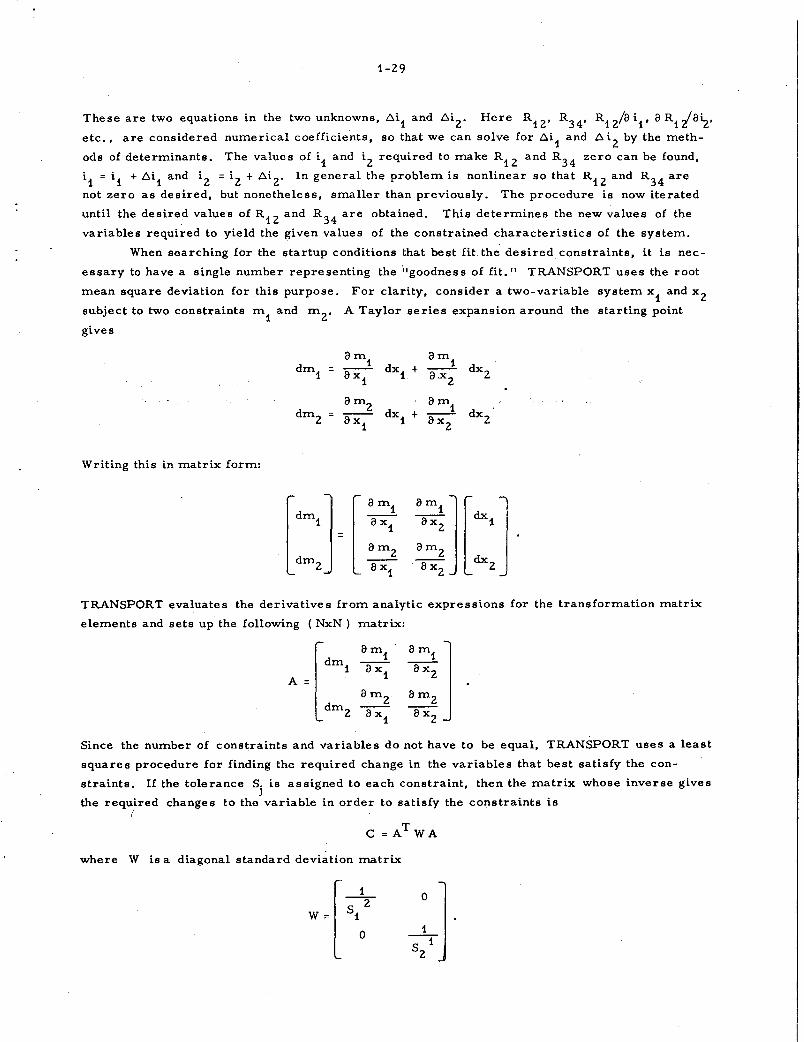
When searching for the startup conditions that best fit. the desired constraints, it is nec­

essary to have a single number representing the "goodness of fit." TRANSPORT uses the root

mean square deviation for this purpose. For clarity, consider a two-variable system x1

and x 2 subject to two constraints m

1 and m

2. A Taylor series expansion around the starting point

gives

dm1

ami dx1 +

ami dx2 a:x

1 a.x2

dm2

8m2

dx1 + 8m

1 dx2 8x1

ax2

Writing this in matrix form:

TRANSPORT evaluates the derivatives from analytic expressions for the transformation matrix

elements and sets up the following { NxN ) matrix:

A= [dm1

dm2

Since the number of constraints and variables do not have to be equal, TRANSPORT uses a least

squares procedure for finding the required change in the variables that best satisfy the con­

straints. If the tolerance S. is assigned to each constraint, then the matrix whose inverse gives J

the required changes to the variable in order to satisfy the constraints is

where W is a diagonal standard deviation matrix

[_1 0] w" \z s:'

1-30

The S.' s have the significance that the jth constant should have the specified value ± S.. Per'-J -- J

forming the indicated multiplication gives a symmetric matrix whose lower triangular part is

'c =

The first row and first column are vectors that give the goodness of fit and negative

one half the gradient of the vector space. The inverse matrix c- 1 will give the required cor­

rection dXj to the variables Xj to satisfy the constraints. The rms deviation to the con­

straints is

0 =J'i (;;\2 J = 1 J J

k

_ Jc(1, t) - k

and the gradient is

gj - 2 C(j, 1)

residuals ...

The differential matrices used by TRANSPORT in calculating the A matrix are given below

for the various types of elements. The differential matrix for a bending magnet whose mag­

netic field is a variable can be written as

L R21 LR11-R12 L pR12-R16

dm L 2 L 1!.. "dl3 = R21---7Ru LR21 pR11 p p

0 0 0

v \) u "1

' 9 5

1-31

If the field gradient n is varied instead, then

L R21 LR11-R12 L p R12-2R16

dm 2 L 1 R21-LR11

w LR21 dw 2 p R11-R26 w

p

0 0 0

where w = .J 1-n in the bend plane or w = ..rn in the non bend plane and the Rjk' s are the usual

first order transformation matrix element for the magnet.. Note that only the dispersive matrix

elements differ for the differential matrices when B or n are constdered variables. For a

quadrupole, either the length or field may be varied. For a variable quadrupole length

2 1 dB where k [ Bp da]. If the pole tip field is variable, the differential matrix is

Variables and Vary Codes

Variables are parameters describing the beam line that the user will allow TRANSPORT

to vary when attempting to satisfy constraints. A variable is designated by a non- zero vary code.

Vary codes make up the decimal part of the unique type code assigned to each magnet type and

may have the values 1 through 9. Each succeeding part of the decimal corresponds to the appro­

priate parameter in the parameter list for the type code, e. g., the first decimal place (.X)

would designate the first parameter as a variable if Xi= 0, the second decimal place (.OX) would

designate the second parameter as a variable if X f. 0, etc. Consider a quadrupole (type code 5.)

whose_ field is variable and is the second parameter on the parameter list, the type code would

be written 5.0X with x = 1, 2, 3, ---9 to specify the field as a possible variable (e. g., 5.01). The

length of the quadrupole is the first parameter in the parameter list and if both the length and

field are variable the type code would be written 5. NM with N, M ;= 1, 2, ----9.

Often it is desirable to tie two or more variables together so that the same change is

made to each variable, An example of this would be a symmetric triplet where the first and

third quadrupoles must have the same field. This is accomplished by using the same digit (not

0 or 1) for the vary code of each quadrupole. A vary code of 0 specifies the corresponding

parameter may not be varied. The vary code 1 specifies the corresponding parameter may be

varied and does not couple to any other vary code of a type code. A vary code of 2 in the first

1-32

decimal part will couple to any other vary code of 2 in the first decimal part of any other type

code but will not couple to a vary code of 2 in the second decimal part of a type code. Similarly

for vary code of 3, 4, 5, 6, 7, 8 and 9. Vary codes 4 and 9 (also 3 and 8; and 2 and 7) will play a

special role if used in the same decimal part of the type codes in that the correction added to

the variable with vary code 4 will be subtracted from the variable with vary code 9, etc. This

antisymmetric coupling can be prohibited by a 13. 50. entry. As an example, consider finding

the location of the horiz.ontal waist following a bending magnet. This may be accomplished by

sliding the waist constraint (10. 2.1. 0 .. 01 card). along the beam line while maintaining the total

beam line length:

3. _____ _

4. L. B. N. 3.4 LL

10. 2. 1. 0 .. 01

3.9 L2. 5. _____ _

3. _____ _

drift length L1 will be varied so

as to place the 10. data card at

the horizontal waist such that

L1 + L2 = constant.

TRANSPORT allows a maximum of 10 variables.

Internal Constraint on Variables

Internal limits are placed on the values that variables may be assigned by TRANSPORT

during optimization in order to prevent the mathematical procedures from assigning non-physical

values to real parameters e. g., negative drift lengths, etc. Table 2 gives the beam element and

the ·lower and upper limits on its variable parameter list. These internal1imits may be altered

by use of the 21. data element. The values specified on the data input need not be within the

limits given in the table. The internal limits are only imposed during computer optimization.

The limits are for whatever units are being used, so if magnetic field is in kilogauss, the vari­

able quadrupoles will be limited to fields values between - 20 and + 20 kilogauss, whereas, if the

magnetic field is in units of tens-of-kilogauss, the variable quadrupoles will be limited to field

values between- 20 and+ 20 tens-of-kilogauss i.e., - 200 to+ 200 kilogauss.

When a user selects the variable metric optimization6 package of TRANSPORT the al­

lowed physical range L1

L2

of each variable j as defined by the internal constraint of the variable

is transformed into a numerically infinite range. If D. is the external variable and x. is its inter-J J

nal value, then

(D.-L1. 1T/2) X. l J

J tan Lz.-Lf. 1T-J J

such that

L1. ~D. ~ L2. J J J

-oo ~ x. ~ + 00 •

J

u ~ 4 9 6

1-33

This scaling of the variables requires a scaling of the gradient such that iff is the rms devi­

ation, then the internally scaled gradient is

IH (L2-L1) g ---j - 8 D. TT • - J J

2 cos

This mapping of the physically restricted range on to the infinite plane allows optimization in a

multidim~nsional space without crashing into limits.

Table 2. Internal constraints on variables.

Element JTYI:~e Variables Lower ~ Lower Upper

BEAM 1 1.111111 .01 1000. Etc.·

POLE 2 2.1 -60. 60.

DRIFT 6 3.1 .1 1000.

BEND 4, 5, 6 4.011 -18. 18. -500. 500.

QUAD 7, 8 5.11 .01 10. -20. 20.

EXTRA 9, 10, 11

ALIGN 12, 13 8.111111 -1. 1. -50. 50.

Repeat three more times

AUX 14 14.111111 None None

SOL 15 1-9.11 None None None None

ROT 16 20.1 -360. 360.

2-1

Section 2 - Standard Data Input

TRANSPORT DATA DECK STRUCTURE

Each TRANSPORT data deck consists of a computer control card record and a TRANSPORT

data deck record, with these two records separated by a end of record mark. The data record

begins with a date and case number card (except the interactive TRANSPORTS, TRAN3 and

TRAN4) and an unlimited number of data cases, each starting with a title card and ending with a

sentinel card (or 73. card).

The input file structure is

Off-line

Date card

1

TITLE

0

73.

73.

On-line

TITLE

0

73.

EOF

The first data card of the off-line TRANSPORTS (TRANZ and TRAN22) must be a com­

ment card called the date card. ~!_h:._ ~ntry on this card will head each run made. Usually the

comment is simply the date or the card may be left blank. The second card must be a case num­

ber card with any numeric entry which will be used as the starting value of the case number.

This case number is automatically incremented for each new case read by TRANSPORT. Follow­

ing these two special cards may come any number of stacked TRANSPORT data cases, each begin­

ning with a title card/option card and ending with a terminator (sentinel or 73 .. ) card. A double

sentinel card terminates the job.

COORDINATE SYSTEM AND SIGN CONVENTIONS

Before describing the detailed data input to TRANSPORT a few words should be said about

the coordinate system and the magnetic field sign conventions used by TRANSPORT.

fields:

Magnetic Field Sign. The following sign convention can be adopted for the magnetic

Quadrupole field positive:

Quadrupole field negative:

Bending magnet field positive:

Bending magnet field negative:

Horizontally converging

Vertically converging

Upward

Downward

2-2

These conventions are true for both positive and negative particles by using a right

handed coordinate system and right hand rule for positive particles with +x axis to left looking

along +z and a left handed coordinate system and left hand rule for negative particles with +x

axis to right looking along +z.

Coordinate System. The spacial coordinates are as follows:

+z axis:

+y axis:

+x axis:

Direction of particle motion.

Vertical displacement upward.

Horizontal displacement, use left or right hand rule depending on sign

of particles. Left hand rule for negative particles and right hand rule

for positive particles.

Energy input. The particle energy can be used as input instead of the momentum by

specifying the rest mass of the particle before a beam card via the 16. 18. data entry. The in­

put of the rest energy must be in units compatible with the momentum units, and thus must fol­

low any unit cards and preceed the beam card, e. g.,

Test energy input of 0. 75 GeV protons

0

15. 1.

1 5. 11. Ge V / c 1.

16. 18. 0.938213

1. X. XP. Y. YP. S. oP/P. 0.750

73.

The use of negative momentum or energy is to change the sign of the particles sent

through a given beam line. If a beam line is set up for a positive particle, negative particles

can be sent through the beam line by setting P = -P. This has the effect of reversing the sign of

all magnetic fields.

DATA INPUT FORMAT

All data input to TRANSPORT is read field free. As each card is read it is printed

into the output stream. After completion of the reading, the entire data array is printed to give

the data index count and names associated with each data line. During Option 0 input the data is

placed sequentially into an array called the data array with location counter I. All data is placed

into this array except vectors (22 element) and arbitrary matrices (25 element) which are stored

in special arrays. A maximum of 300 numbers are allowed in the data array.

·The field free input may begin in any column. All entries after a $ are ignored by

TRANSPORT and may be used to place comments on the data cards. An unlimited number of

conunent cards, beginning with a $ may be placed anywhere in the data deck. Alpah-numeric

blocks are separated by blanks and/or commas. Each data line (TRANSPORT element) is

u j - 7

2-3

entered .on one card except possibly the 1, 12, and 25 elements, as explained elsewhere.

Numeric blocks consist of numbers or group of numbers which constitute the data input

to TRANSPORT. These numbers may be integers (which will be considered as having unspec­

ified decimal points and as such really be floating point numbers) floating point numbers, expo­

nential numbers in any mixed order with the provision of repetition by use of the repeat specifica­

tion (R).

Example:

Integers

Floating points

Exponentials

Repeats

- 1. 2, 25, etc. (interpreted as 1. 2. 25.)

3.074 -5.2540 +. 667 -0.0123

- +2.0123E-6, 1.2345E+4 1E6, +1E+4 etc.

- OR6, 6. 7502R2 1.42E -3R4

OPTION 0, THE BASIC DATA DECK

The first card of each TRANSPORT data case of a title card and the second card is an

option card.

Option 0 specified on the second card of a data deck is the standard data input option and

specifies that the data.following consists of a type code and parameter list as will be described

shortly. The data read under the Option 0 input will form the nucleus of the Options 1, 2, 3, 4 and

5 data, should they be used.

The naming of a data line is optional. If one names the line, the name must begin with an

alphabetic character and should not exceed six characters in length. If N is the usual number of

entries of the particular data line, the name would be entered as the N + 1~ entry.

Two different types_ of input data cases can_ be used ~th TRANSPORT .. ~he Option 0

cases define the user beam line, specifying the various magnets, input-output options, vectors

and beam to be transformed, etc. The other options (1, 2, 3, 4, and 5) operate on the basic data

deck as defined by Option 0. These other options allow the data deck to be modified in various

ways and the calculations reperformed with the modified deck.

The basic beam line (Option 0) deck is built from the 27 different element types available

to TRANSPORT. These 27 element types are presented in Table 3.

Element t e

1

2

3

4

5

6

7

8

9

10

11

1"2

13

14

15

16

17

18

19

20 ------- 21

22

23

24

25

26

27

2-4

Table 3.

Meaning

Beam ellipsoid input

Bending magnet pole face rotation

Drift length

Bending magnet

Quadrupole magnet

Slit

Axis shift

Misalignment

Repetition

Constraint

Accelerator energy gain section

Beam correlation

Output specification

Arbitrary matrix

Unit change

Parameter input

Second order

Sextupole magnet

Solenoid magnet

Beam rotation - -

Stray field and miscellaneous input

Particle vectors

Particle separator

Plot options

Calculated matrix

Space charge

RF buncher

These elements will be described in more detail later.

2-5

The Option 1, 2, 3, 4, and 5 data decks allow the basic Option 0 data set to be manipulated

or alt.ered in the following manner:

Option 0

Option 2

ALINE

ALTER

DLINE

FIX

NAME

MOVE

PUNCH

POLYG

REVERSE

Option 3

Option 4

Option 5

Input new beam and/ or vectors

Add a line to the data

Alter a parameter in the data

Remove lines from the data

Fix variables and remove constraints

Rename the data

Move several lines of data

Write data out to tape 7

Calculate acceptance polygon

Reverse order of data in data array

1, 2, 3, or 4. dimensional chi- square search

Second order plotting and histrograms

Calculate acceptance polygons

These operations will be described after the detailed description of the 27 basic TRANSPORT

elements which follows.

Data is read by subroutine READX called from readin.. The data. is placed sequentially

into an array called data with location counter I. All data is placed into the data array except

vectors (22) and arbitrary matrices (25.) which are stored in special arrays. As the data is read

it is printed, each type on a line. The read in of data continues until a sentinel or 73_. data card

is encountered.

The data array is then printed out in its entirety, giving the I counter as calculated by

readin in the left most column, the data name as specified by the user or calculated by the code

in the absence of a user name, followed by the type code and parameter list for each data card

read. The reading of a type code 73. signifies the conclusion of the data input and transport then

prints the total number a data numbers stored in the data array. This number must not exceed

300.

The I counter is the location of the type code of each data element and will be used by the

Option 2 and Option 3 data input, i.e., if one wishes to refer to the magnetic field of the quadru­

pole (type code 5.) at I count 37 he will specify I count of 39, (37 + 2).

I Name

35 (L1) 37 (Qi) 41. (L2)

Type code Parameter list

3.0 L.

5. 000 c: B. A.

3.0 1------------~---t__---------~i ~~~~~ j~ I count 38 I count 37

2-6

I I

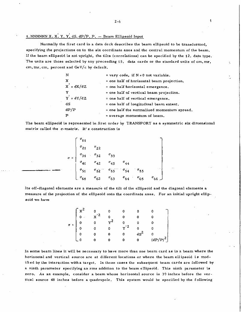
1. NNNNNN X. X. Y. Y. dS. dP /P. P. - Beam Ellipsoid Input

Normally the first card in a data deck describes the beam ellipsoid to be transformed,

specifying the projections on to the six coordinate axes and the central momentum of the beam.

If the beam ellipsoid is not upright, the tilts (correlations) can be specified by the 12. data type.

The units are those selected by any preceeding 15, data cards or the standard units of em, mr,

em, mr, em, percent and GeV/c by default.

N

X I

X = dX/dZ

y I

Y = dY/dZ

dS

dP/P

p

= vary code, if N = 0 not variable.

= one half of horizontal beam projection.

= one half horizontal emergence.

= one half of vertical beam projection.

=one half of vertical emergence.

= one half of longitudinal beam extent.

= one half the normalized momentum spread.

=average momentum of beam.

The beam ellipsoid is represented in first order by TRANSPORT as a symmetric six dimensional

matrix called the a-matrix. It' s construction is

(111

(121 (122

(131 (132 (133 (1 =

(141 (142 (143 (144

(151 (1 - --52

(1- --53

(1 --54 (155

- (16i (162 (163 (164 (165 (166

Its off-diagonal elements are a measure of the tilt of the ellipsoid and the diagonal elements a

measure of the projection of the ellipsoid onto the coordinate axes. For an initial upright ellip­

soid we have

xz 0 0 0 0 0

0 x'2 0 0 0 0

0 0 y2 0 0 0 (1 = y'2 0 0 0 0 0

0 0 0 0 dS2

0

0 0 0 0 0 (dP/P)2

In some beam lines it will be necessary to have more than one beam card as in a beam where the

horizontal and vertical source are at different locations or where the beam ellipsoid is mod­

iii ed by the interaction with a target. In these cases the subsequent beam cards are followed by

a ninth parameter specifying an rms addition to the beam ellipsoid. This ninth parameter is

zero. As an example, consider a beam whose horizontal_ source is 39 inches before the ver­

tical source 48 inches before a quadrupole. This system would be specified by the following

u v u u ~~ I i.J ~ ~ 9 9

2-7

data cards: I

1. X. X o. 0. 0. dP/P. P.

3. 39. I

1. 0. o. Y. y 0. 0. 0. 0.

3. 48.

5. 16.75 4.315 4.

As another example, consider a beam that passes through a target resulting in a multiple scat-

. tering increase in the phase space and an reduction in the beam momentum. The correlations

are unaffected. Then the data card:

1. I

dX. dX . I

dY. dY. dl. o(dP/P). oP. 0.

With nine parameters rather than the usual eight placed at the target location produces an rms

alteration of the beam. The beam would then be given by the matrix.

u= (unaltered)

(dS) 2 +(dl) 2

(unaltered) (dP/P)2+(o(dP/P)) 2

and transformed at a momentum P + o P. (o P would be negative).

The beam card may also be used to input betatron functions. In order to do this, the

phase area in the two decoupled phase planes must be inserted before the beam card via a 21. 0.

EX. EY. card, e.g.'

21. 0. E E . X y

1. 13x· a . 13y· a . o. 0. P. X y

Here a and 13 are the betatron functions and E , E are the phase areas divided by tr and 2 X y

y = (1 +a )/13. The units will be the standard TRANSPORT units or as altered by any 15. data

entries. In the absence of any unit change, the 13' s are in cm/mr, y' s in mr/cm, a's dimen­

sionless, and E's in cm-mr.

The betatron functions along the beam line will be printed in a summary table, at the

end of the TRANSPORT run. The Betatron functions are converted to the standard transport

u-matrix and are transparent to TRANSPORT, only being used for input-output convenience by

the user.

2-8 2

2. N p. B2. Magnet Pole Face Rotation

Non-normal entry or exit into or from a bending magnet may produce first order focusing

in either plane. The required parameters are the angle between the normal to the paraxial tra­

jectory and the face plane of the magnet and the magnetic field inside and outside the magnet.

The field inside the magnet will be taken from the magnet data card (4. card) and the field out­

side the magnet is specified as the third parameter B2 and is normally zero.

N = vary tag, ~ is variable if N -:F 0.

~ = angle between normal to paraxial trajectory and

magnet face in degrees. Angle with same sign

as magnetic field will give positive vertical

focusing.

B2. = field outside magnet, normally zero.

In a sequence of 2. and 4. data elements, a 2. element will be considered a entry rotation e. g.,

in the sequence 4., 2., 4., 2., 4. the grouping is (4. ), (2., 4), (2., 4.)

where

and

with

The matrix representation for the 2. element is

R=

1 0 0 0 0 0

tan!3 1 0 0 0 0

p

0 0 1 0 0 0

0 0 -tan({3-y)

1 0 0 p

0 0 0 0 1 0

0 0 0 0 0 1

y=K (~) 1+sin2{3

[1 -K1 K (g) tan~] . 1 p cos~ 2 p

p = P/e (Bm -B2)

K 1 = fringing field parameter input by 16. 7. K1

.

K 2 =fringing field parameter input by 16. 8. K2

•

B = Bending magnet field input by 4. L. B • N. m m

g = haU vertical gap of bending magnet input by 16.

P = particle momentum.

Default value = 0.5

Default value = 0.

5. g.

The pole face rotation may be varied by the program in attempting to satisfy the system

constraints if the vary tag, N, is non-zero. Internal program constraints will constrain the

absolute value of~ to be less than 60 degrees if~ is varied.

A pole face rotation (2. element) normally preceeds or follows a bendi.ng magnet (4. el­

ement). The only data cards which may be placed between a 2. and 4. data card describing a

"¥ - i

2-9 3

magnet are up to fove 13. cards or five 2. cards. Any other· card will cause a non-fatal error.

The following sequences are allowed.

2. {3. 0. -2. {3. o. 13. 8. 2. {3. 0.

4. L. B. N. -2. (3. o. etc.

13. 8. -2. {3. o. 2. {3. 0. 13. 8.

4. L. B. N: 2. {3. 0.

The sign convention for {3 is shown below

XBL752-2407

with {3 giving vertical focusing when it has the same sign as the magnetic field.

3. N L. Drift Length

A field free region of length L is specified by the 3. data element. The units of L are

specified as the eighth unit and is normally meters. The matrix is:

1 L 0 0 0 0

0 1 0 0 0 0

0 R

0 1 L 0 0

0 0 0 1 0 0

0 0 0 0 1 0

,0 0 0 0 0 "1

The drift length may be varied if N --F 0, i.e., 3.1 or 3.2 etc. designates a variable drift length

of initial value L. The internal constraint built into TRANSPORT will place a lower limit on L

of 0.1 units and an upper limit of 1000 units. If L is not a variable (N = 0) L may take any real

value - «> < L < ao

2-10 4

4. OKM L. B. N. Bending Magnet

A 4. data card specifies a bending magnet of normal entry and exit. If the paraxial tra­

jectory does not make normal entry and exit a pole face rotation must be specified by a 2. data

element. A negative length indicates a vertical bend. An upward field is taken as positive.

K =magnetic field vary code, if K = 0 B is not variable.

M =field index vary code, if M = 0 N is not variable.

L. = Effective length of field along trajectory in the same

units as drift length, unit (8), normally meters.

B. = Average magnetic field along paraxial trajectory in

units of unit (9), normally kilogauss.

N. =Magnetic field index R(dB/dX)B- 1 where R is the radius

of curvature of the particles and dB/dX is the trans­

verse gradient.

The first order matrix representation of a bending magnet is:

KL i sinKxL 0 0 0 1 cos --2(1-cos K L)

X K X X p X

-K sinK L cos K L 0 0 0 +sinK L X X X p X

X

0 0 cosK L ~ sinK L 0 0 y y y

R

0 0 -K sinK L cos k L 0 0 y y y

1 sinK L 1 0 0 1 + 3(K L-sinK L) -K p X

--2- (1-cosKxL) K X X

X -Kxp p X

0 0 0 0 0 1

where p =radius of curvature = P/eB and

2 -2 Kx = (1-n) p

2 -2 K = np

y

The parameter list for the bending magnet may be changed by the 16. 21. data option so that any

combination of length, bending angle or magnetic field may be used, see the 16. data input.

For realistic calculations a vertical gap correction must be made for the fringing field of

bending magnets. For wedge magnets, this can be accomplished by use of the 16. 22. 1. data

card which will produce a zero angle fringe field matrix at the entrance and exit of all subse­

quent bending magnets until explicitly tuned off by another 16. 22. data specification. Alterna­

tively, a 2. 0. fringe matrix may be explicitly given at the entrance and exit to the wedge ·mag­

net.

A rectangular magnet that is symmetrically oriented so that the entrance and exit angles

are each half the angle of bend may be specified by a 16. 22. 2. data card. Once the rectangular

magnet specification is given, it will remain in effect until changed by a different 16. 22. data

entry.

2-11 5

5. NM L. B. A. Quadrupole Magnet

A quadrupole produces first ordei: focusing without deflection of the beam. A positive

fieid, B, indicates a horizontally focusing lens while a negative field indicates a vertically

focusing lens.

N Length of quadrupole variable if N -:jc 0.

M Magnetic field of quadrupole variable if M -:jc 0.

L. Effective magnetic field length along Paraxial trajectory in the same units as drift

lengths, unit (8).

B. Magnetic field at pole tip of quadrupole in units of unit (9) normally kilgrauss.

A. One-half the pole to pole gap, i.e., the radius of the inscribed circle in the same

units as horizontal beam displacement, unit (1).

The first order matrix representation of a quadrupole magnet is

cosK L ~ sinKxL 0 0 0 0 X

-K sinK L cosK L 0 0 0 0 X X X

0 0 cos K L If-sinK L 0 0 y y y

0 0 -K sinK L cosK L 0 0 y y y

0 0 0 0 1 0

0 0 0 0 0 1

where

K2 B X Ar

. K2 B - Ar y

r magnetic rigidity of beam (r Bp ~). e

6. J. X. Y. Slit

This element is used to introduce appertures along the beam line for display and

polygon calculation. It has no effect on the transformation matrix or beam matrix but will in­

teract with the polygon calculation and vector tracking if the vectors exceed the specified aper­

ture and the 16. 14. option is selected. The interpretation of X andY is designated by the

value of J and listed below:

J = 0

J = 0

X=i.

X = 2.

J = 0 X = 3.

J = 1 X

J 2 X. Y.

Updates beam. Reinitalizes RC transformation matrix. This is not a slit.

Initiates the RC2 matrix. This is not a slit.

Initialize R3 matrix.

X = Horizontal half width of slit if y = 0.

X and Y are the rectangular half apertures to be associated with the first

element following which possesses length.

J = 3

J = 4

J = 5.

X.

X. Y.

X. Y.

2-12

X =vertical half width of slit if y = 0.

X and Y are the rectangular half widths of the slit of zero length.

X and Y are the half widths of an elliptical slit. Only used with vector

16. 14. option.

7

J 6. X. Y. X a.nd Y are the elliptical half apertures to be associated with the first element

following which possesses length. Only used with vector 16. 14. option.

1 1

7.NNNNNN dX. dX. dY. dY. dS. doP/P Axis Shift.

This element introduces a shift in the location of the beam centroid and introduces an up­

date of the RC transformation matrix. The units are the same as for the beam matrix (1. data

element).

N = vary code, if N = 0 parameter not variable

dX =horizontal phase space displacement of beam centroid 1

dX = horizontal divergence displacement of beam centroid

dY = vertical phase space displacement of beam centroid 1

dY = vertical phase space divergence displacement of beam centroid

dS = longitudinal phase space displacement of beam centroid

odP/P =momentum displacement of beam centroid

The axes shifts (X.) are added to the beam centroid vector (seventh column of u matrix) and J

added quadratically to the beam ellipsoid. The transformation for i = 1, 6: J =1, 6 is

u.. u .. + X. X. + u.7

X. + u.7

X. 1J 1J J 1 1 J J 1

On output, the centroid transformations are

r .. 1J

(u .. - u. 7

u. 7)/J (u ..

1J 1 J 11 2) ( 2) 1 • .L u. 7 u .. + u.

7 t-

1 JJ J

The element has no effect on the value of the several transformation matrices or on vector

calculations.

8. VVVVVV X. e. Y. <J>. S.lj!. NMP. Misalignment

The 8 element allows the user to investigate the effect upon the beam of a misalign­

ment of an individual magnet or group of magnets by either uncertainties in their locations or

by a deliberate displacement. The misalignment element does not effect the transformation

matrix and so has no effect on the transformation of particle vectors except it does produce an

update of the RC matrix. The input parameters are given below and assume the horizontal and

vertical phase planes are in the same units.

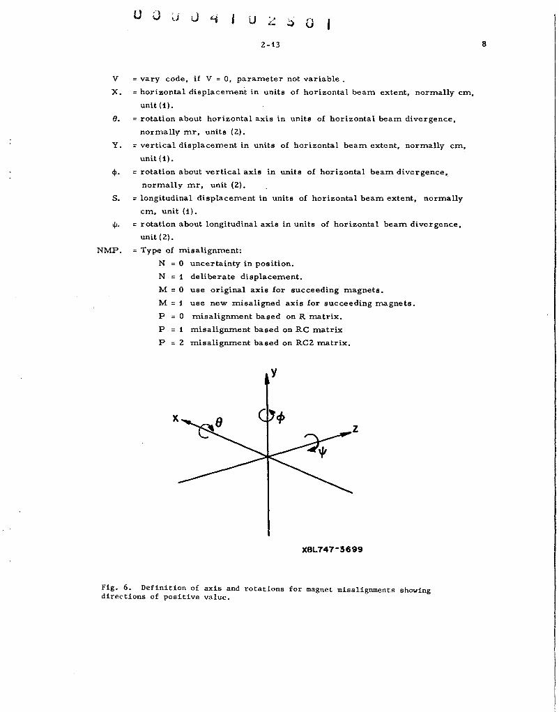
0 J J J ~

2-13

V = vary code, if V = 0, parameter not variable .

X. = horizontal displacement in units of horizontal beam extent, normally em,

unit ( 1).

8. = rotation about horizontal axis in units of horizontal beam divergence,

normally mr, units (2).

Y. = vertical displacement in units of horizontal beam extent, normally em,

unit (1).

cjl. = rotation about vertical axis in units of horizontal beam divergence,

normally mr, unit (2).

S. = longitudinal displacement in units of horizontal beam extent, normally

em, unit (1).

~· = rotation about longitudinal axis in units of horizontal beam divergence,

unit (2).

NMP. = Type of misalignment:

N = 0 uncertainty in position.

N = 1 deliberate displacement.

M = 0 use original axis for succeeding magnets.

M = 1

p = 0

p = 1

p = 2

use new misaligned axis for succeeding magnets.

misalignment based on R matrix.

misalignment based on RC matrix

misalignment based on RC2 matrix.

y

XBL747-3699

Fig. 6. Definition of axis and rotations for magnet misalignments showing directions of positive value.

8

2-14

The various misalignments may be altered by TRANSPORT by flagging them as variables by

making the appropriate V non-zero, e. g., if the value of the horizontal displacement is to be

varied to produce a centroid shift of 0.1 inches the following data pertains:

find misalignment for centroid

shift of 0.1

9. N: Repetition

0

1. XX' YY' S dp P

6. 0. 1.

5. L B A

8.1 0.9 0 .0. 0. o. 0. 100.

10. 7. 1. 0.1 .01

find misalignment for centroid

uncertainty of 0.1

0

1. o. o. o. o. o. o. p

6. 0. 1.

5. L B A

8.1 0.9 0. 0. 0. o. 0. 1.

10. 7. 1. 0.1 .01

9

II a group of data elements is to be repeated, an economy in input is provided by the

repetition element 9. This card specifies that all the data following it up to a 9. 0. data card

shall be repeated N times. These repetition groups may be nested four deep. Consider the fol­

lowing example showing two identical data structures of the same beam:

3. __ _ 5. __ _ 3. __ _ 9. 2. 2. __ _ 3. 4. __ _ 5.

13. __ _ 3. __ _ 2. __ _ 4. __ _

13. __ _ 3. __ _ 5. __ _ 3. __ _ 5. __ _ 3. __ _ 5. __ _

9. 2. 3.

o.J 2. 4.

13. 9. 9. 2.1 3. 5. 9. o. __

3. __ _ 9. o. 2. __ _ 4. __ _

13. __ _ 3. __ _ 2. __ _ 4. __ _

13. __ _ 3. __ _ 5. __ _ 3. __ _ 5., __ _

o u· d J ·- 0 '

2-15 10

10.NJ. K.X. oX. Contraint

TRANSPORT allows many quantities to be constrained. These divide into three general

types, constraint of non-matrix system parameters, constraints on system matrices and con­

straints on linear combinations of system matrices. J., K. specify which quantity is to be con­

strained to the value X:!:: oX. The decimal part of the type code, N, specifies if the constraint

is an actual constraint N = 0; upper limit N = 2; or a lower limit N = 1.

Of the first type of constraint, only the length of ·the system with variable drift lengths

may be constrained.

Of the second type of constraint, TRANSPORT allows constraints on the beam matrix

(a-matrix), the accumulated transformation matrix 1 (RC-matrix), the accumulated transfor­

' mation matrix 2 (RC2-matrix), and the betatron functions J3, a, y, TJ and TJ •

Linear combination of matrix elements are often constrained and comprise the third

type of constraint. For any matrix between two waists, the phase advance is:

If the two waists are identical

-1 1 IJI = cos 2 (R11 + R22>.

Or the linear combination of transformation matrix elements

K M(A, B) +M (C ,D) = x:!:: ox

can be constrained, where M is the RC, RC2, or SI matrix for the data input of 16. 25. 1., 16.

25. 2., or 16. 25. 3. respectively, and J = ABCD. When the general phase advance is to be

constrained the 16. 25. 4. data entry is used. Then

where

1J. 4~ cos- 1 {RC(A,A) RC(B, B)+ RC(A, B) RC(B,A)}

2-16

Type of constraint Constrained parameter

System length L

Auxiliary accumulated RC2(J, K) Transfer matrix

Betatron phase angle <IJK

Transformation matrix RC(J, K)

Beam matrix u(J, K) Projections Covariance

Correlation of- beam rjk

Betatron functions f3x' a.x' 'Yx

f3y' a.y' 'Yy

~· ~p· "\r' Tlyp

Combination of matrix K RC(A, B)+RC(C,D) element~, K is floating point.

Value of J and K

0 0

-(J +20), K

-(J +10), K

-J,K

J,K J=K J>K

(J +10), K

(J +20), K

ABCD,K

Comments

J,K=1, 2, 3,---6

cos(21Tcj>JK) = 1/2

( RC(J, J) +RC(K, K))

J may equal 7 for centroid of beam

11

(J +20, K) =(21 ,1 M22, 1 ), (22, 2)

(J +20, K) =(23, 3),(24,3), (24,4)

(J+20, K) =(21 ,6), (22,6), (23, 6), (24, 6)

11. L. DP. Phase. WAVEL. Accelerator Energy Gain Section

The effect of an accelerator section is simulated by the 11. element. This element

alters the beam momentum, size and divergence. The matrix for the accelerator for a fully

relativistic beam is

1 LP ln ( 1+ dP cosp) dPcoscj> P 0 0 0 0

0 p

0 0 0 0 P+dPcoscj>

0 0 1 LP ln[dPcosp dP(cos~ P + 1] 0 0

0 0 0 p

0 0 P+dPcoscj>

" I !

0 0 0 0 1

Ptd;co•~ J 0 0 0 0 dP sinp21T

( P+dP coscj>)"-

2-17 12

L length of accelerator cavity in units specified by unit (8), normally meters.

dP momentum gain in units specified by unit (11), normally GeV/c.

Phase phase of cavity in degrees.

Wavel = RF wave length in units of longitudinal spread specified by unit (5),

normally CM.

If the particle rest mass has been defined by the 16. 18. RESTM. Card dP and P of the beam

will be interpreted as the energy rather than momentum.

12. (r .. , i = 2, 6, J = 1, i -1) Beam Correlatic)n l

The beam ellipsoid may be tilted in any of the 15 phase planes corresponding to the six­

dimensional ellipsoid. These correlations are specified by the 12. data element giving the 15

r .. where lJ

r .. -lJ

(1 •• 1]

These correlations are dimensionless and are given in the following order;

The 12. data card must immediately follow the beam card whose parameters qkk will be used

to calculate the q •. from the given r ..• lJ lJ

The input for the 12. element may appear on one or two data cards. If two data cards

are used, the first card must have exactly eight entries. For example, all three of the following

would give identical results:

12. r21 0 0 0 0 r43 0

0 0 0 r 61

or 12. r21 OR4 r43 OR r 61 OR4 NAME

or 12. r21 OR4 r 43 OR4 r 61 ·

13. J. Output Specification

The 13. element allows the user to suppress various output normally generated by

TRANSPORT or to initiate output not normally generated. The action introduced as listed below

for the various values of J.

2-18 13

J. MEANING

1. Temporary override of suppression of beam ellipsoid output.

2. Suppress beam ellipsoid output. 2.1 will also suppress beamline graph.

-2. Suppress all output on first run through before optimization. Normal output after optimiza­

tion with beam ellipsoid output suppressed except where specified by 13. 1. or 13. 3.

option.

3. Permanent override of beam ellipsoid output suppression.

4. Print accumulated transfere matrix, RC, from last beam update and total accumulated

transfere matrix from beginning of beam line if the RC matrix has been updated.

5. Aperture transformation orgin. Specifies location on beamline where all apertures sub­

sequently encountered will be transformed back to in the horizontal and vertical phase

space.

6. Print phase space aperture polygons at the locations of the 13. 5. and/or 13. 6. data cards

during Option 5 calculations.

7. Momentum (energy) spectrum. Print phase space aperture polygons at the locations of the

13. 5. and/or 13. 7. data locations at each of the momentum specified by the 24. 4. data

card during performance of Option 5 calculations.

8. Print the transformation matrix, R, of the preceding element.

9. Sets RiP true

10. Quadrupole aperture constraint flag. Generates a beam projection constraint (10. 1. 1. or

10. 3. 3.) at entrance and/or exit of any quadrupole if the X or Y beam projections exceeds

the quadrupole aperture. This option replaces the conditional constraint at quadrupole en­

trance and exit as shown below:

13. 10. t l 10.2 1. 1. A1 A1/10

10.2 3. 3. A1 A1/10

5. L B A1 5. L B A1

l 10.2 1. 1. A1 A1/10

10.2 3. 3. A1 A1/10

1t.2 1. 1. A2 A2/10

10.2 3. 3. A2 A2/10

5. L B A2 5. L B A2

! 10.2 1. 1. A2 A2/10

10.2 3. 3. A2 A2/10

~ 11. CalComp envelope trace - not available

12. CalComp layout - not available

20. Initalize misalignment pivot matrix R

21. Initalize misalignment pivot matrix RC

0 u 0 0 4

2-19

22. Initalize misalignment pivot matrix RC2

24. Print transform matrix 2, RC2 matrix. This matrix originates as a unit matrix at the

location of a 6. 0. 2. data card and may be constrained.

14

25. Suppress vector output. This does not terminate vector transformations so output may be

requested further along the beam line by the 13. 27. or 13. 26. data cards.

26. Permanent override of vector output suppression.

27. Temporary override vector output suppression so as to print vector output at this location.

28. Suppress print out of transformed aperture polygon plots but do not suppress polygon

vertices or solid angle print out.

29. Suppress aperture calculation at location of 13. 5. data cards plot the polygons.

30. Produce aperture calculation at location of 13. 6. or 1.3. 7. data card, plot the polygons.

31.. Adjust horizontal vista phase plot scale so vectors and beam ellipse are within boundary.

32. Adjust vertical vista phase plots scale so vectors and beam ellipse are within boundary.

33. Plot phase space ellipse without centroid shifts at locations specified by 24. ijkl.

34. Plot beam line without centroid shifts if a 24. 0. card is used.

40. Print the RC and R matrix after every element possessing a matrix. Turn off RC, R

matrix output with A 13. -40. data entry.

42. Print the RC matrix scaled by the second order sigma (beam) matrix.

45. Print the polygon transformation matrix originating at the 13. 5. data location.

46. Suppress projection of x, y onto global coordinate system.

48. Print first order R matrix suppressing second order print out.

49. Print out optimization matrix, i.e., a C/a Vk.

50. Uncouple anti-connected variables, i.e., vary codes (9, 4), (8, 3) and (7, 2) are no longer

coupled.

NIJK. used by second order vista transport (TRAN32) to store element T(IJK) in vector position

N. The value of N is given in table below.

N ~ector number M 1 2 3 4 5 6

Horizontal plane 1 3 5 7 9 11

Vertical plane 2 4 6 8 10 12

14. NNNNNN R(J, 1). R(J, 2). R(J, 3). R(J, 4). R(J, 5). R(J, 6). J. Arbitrary Matrix

An arbitrary transformation matrix may be specified by either the 14. or the 25. data

element. The 14. data element defines a unit matrix with one or more non-unit matrix rows J

given by the one or more successive 14. data cards. The units of the matrix elements are those

appropriate for the units selected for the beam card (data element 1.). The matrix elements

may be varied by making the appropriate N non-zero, e. g., if R(2, 2) is to be varied the data

card would be 14.01 R21

• R22

. R23

.R24

.R25

.R26

.2. As an example, consider a typical bending

magnet matrix with rows 1, 2, 3, and 4 of non-unit matrix structure:

14. R11. R12. o. o. o. R16. 1.

14. R21. R22. o. o. 0. R26. 2.

14. o. 0. R33. R34. 0. 0. 3.

14. 0. 0. R43. R44. 0. o. 4.

2-20 15

The rows number is given by the eighth parameter J. Rows 5 and 6 will be zero except

for R(5, 5) = R(6, 6) = 1. If two arbitrary matrices are to follow each other they must be

separated by some non-14. data card, such as a 13. or 16. card.

The units of the arbitrary matrix may be confusing if one is working in a non­

natural set of units. This confusion can be reduced by recalling the matrix expansion of a

particle vector:

If the arbitrary matrix has been calculated in natural units, say em, radians and

' fractions for x,x and dP/P and is to used in transport with the standard units of em, mili-

radians, and percent, then

R

0 0

15. J. DIM. X. Unit Changes

TRANSPORT can work in any set of units. The units that will be used in the ab­

sence of an explicit unit change are called standard units; these are as shown below.

Quantity

Horizontal extent

Horizontal divergence

Vertical extent

Vertical divergence

Longitudinal spread

Momentum spread

Not used

Drift length

Magnetic field

Mass

Momentum of beam

Sumbol Code

X ' X

y

' y

dS

dP/P

L

B

M

p

number Standard unit

1 em

2 mr

3 em

4 mr

5 em

6 percent

7

8 meters

9 kilogauss

10 electron mass

H GeV/c

When N units are to be changed the unit cards must be preceded by a 15. N. X. data

card specifying that N 15. data cards follow. If X is nonzero the units will be restored to the

standard values before processing the N units change cards. This allows a restoring of any

unit changes made in previous data decks. Once a unit change has been made, it will remain

until explicity changed again, so it is not necessary to change units in each data deck pro­

cessed by TRANSPORT. The meaning of the parameters on the 15. data card are:

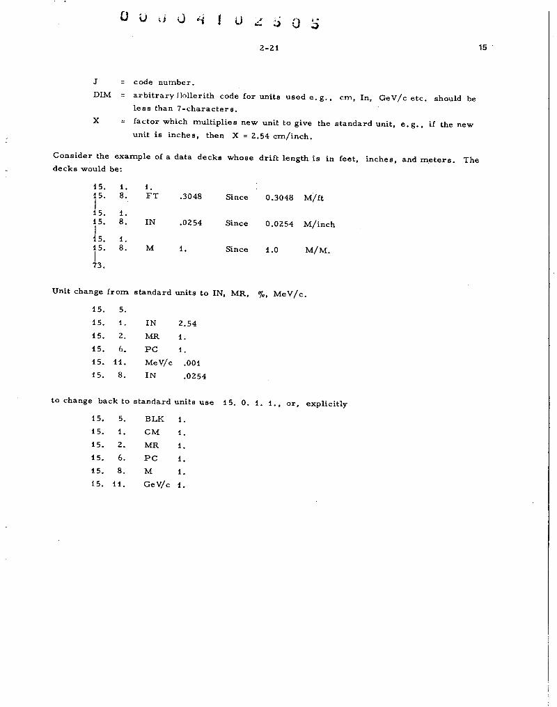
0 u u J u 0

2-21

J code number.

DIM arbitrary Hollerith code for units used e. g., em, In, GeV/c etc. should be

less than 7-characters.

X factor which multiplies new unit to give the standard unit, e. g., if the new

unit is inches, then X = 2.54 em/inch.

Consider the example of a data decks whose drift length is in feet, inches, and m.eters. The decks would be:

15. 1. 1. 15. 8. FT .3048 Since 0.3048 M/ft I 15. 1. 15. 8. IN .0254 Since 0.0254 M/inch

15. 1. 15. 8. M 1. Since 1.0 M/M. I 73.

Unit change from standard units to IN, MR, o/o, MeV/ c.

15. 5.

15. 1. IN 2.54

15. 2. MR 1.

15. 6. PC 1.

15. 11. MeV/c .001

15. 8. IN .0254

to change back to standard units use 15. 0. 1. 1., or, explicitly

15. 5. BLK 1.

15. 1. CM 1.

15. 2. MR 1.

15. 6. PC 1.

15. 8. M 1.

15. 11. GeV/c 1.

15

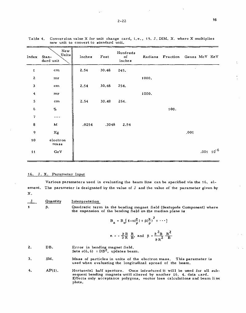
2-22 16

Table 4. Conversion value X for unit change card, i.e., 15. J. DIM. X. where X multiplies new unit to convert to standard unit.

Index

1

2

3

4

5

6

7

8

9

10

11

Stan­dard unit

em

mr

em

mr

em

o/o

M

Kg

New Units

electron mass

GeV

Inches Feet

2.54 30.48

2.54 30.48

2.54 30.48

.0254 .3048

Hundreds of

inches

245.

254.

254.

2.54

Radians

1000.

1000.

Fraction Gauss MeV KeV

100.

.001

.001 10- 6

16. J. X. Parameter Input

Various parameters used in evaluating the beam line can be specified via the 16. el­

ement. The parameter is designated by the value of J and the value of the parameter given by

X.

J Quantity

1 f3.

2. DB.

3. SM.

4. AP(1}.

Interpretation

Quadratic term in the bending magnet field (Sextupole Component} where the expansion of the bending field on the median plane is

B z

X X 2 =B[1-n(-}+f3(-} +···]

0 p p

a B R a 2B Rz n = - a R B' and f3 = a Rz If"

Error in bendin~ magnet field. Sets u(6, 6} =DB , updates beam.

Mass of particles in units of the electron mass. This parameter is used when evaluating the longitudinal spread of the beam.

Horizontal half aperture. Once introduced it will be used for all sub­sequent bending magnets until altered by another 16. 4. data card. Effects only acceptance polygons, vector loss calculations and beam line plots.

5.

6.

7.

8.

9.

10.

11.

12.

13.

14.

15.

16.

17.

18.

19.

20.

u u d u ~ ~ 0 6

AP(2)

LC.

FRi.

FR2.

RDL.

RDB.

RDT.

RAB1.

RAB2.

FOCLTL.

APFILL.

LENGTH.

EREST.

MBE

BSEPR.

2-23 16

Vertical half aperture. Once introduced it will be used for all subse­quent bending magnets until altered by another 16. . data card. This option produces an important correction to the matrix calculation for a 2. element which includes the effect of a finite fringe field.

Input of accumulated length of system. Normally used to give length up to the starting point of current beam line.

Fringing field correction for trajectory bending in magnet fringe field, normally FR1 = 0.5.

+«>

FRI = s B (z)(B -B (z)) Y 0 Y dz

Bz g 0

g is the vertical half gap given by a 16. 5. g. card.

Fringing field correction for trajectory bending in magnet fringe field, normally zero.

Introduces a random gaussian uncertainty in drift length of standard deviation RDL.

Introduces a random gaussian uncertainty in quadrupole fields of standard deviation RDB.

Introduces a random gaussian uncertainty in beam rotation of standard deviation RDT.

Curvature of the entrance face of a bending magnet (reciprocal of radius of curvature) taken as positive for convex curvatures.

Curvature of the exit face of a bending magnet. Taken as positive for convex curvatures. Producing a sextupole strength k2L = -.Sh(RAB) SEC3(3. s

' Causes seventh component of vector to be set to system length if vector exceeds an aperture. The length will be positive if the exceeded aperture is horizontal and negative if vertical.

Rotates the focal plane so second-order aberrations may be printed on the focal plane.

Specifies the factor by which the quadrupole aperture (gap on 5. data card) is to be multiplied in calculating of acceptance polygons and beam line plotting. This option has no effects on matrices or vectors and does not affect the gradient of the quadrupole.

Length of following element. Use to give length to a magnetic element whose matrix is given by a 14. or 25. element.

When EREST=Rest energy of particle the eighth parameter on the beam card will be the particle kinetic energy rather than momentum. Also the momentum spectrum is converted to an energy spectrum. (24. 4.)

When doing betatron functions, plot betatron function if MBE = 1.

Separator action flag. BSEPR = -1 normal transformation of beam and vectors

0 shift vectors = 1 shift beam.

21. ACP3.

22. ACP2.

22. ACP2.

23. VEC.

25. KONGARN

26. FE31.

27. RMSDEV.

28. K STEPRM.

29. OPTYPE.

30. I WRITE.

31. CLOCK.

32. ICNVRG.

33. IRNDM.

2-24 16

Specifies the parameter interpretation for a bending magnet. Normally a bending magnet is specified by the length L, bend field B, and field index N. Often a user knows the length Land angle of bend A. In order to ease input the 16. 21. option allows any combination of L, B, or A.

ACP3 = 0 ACP3 = 1 ACP3 = 2

Bending magnet parameters Bending magnet parameters Bending magnet parameters

4. L. B. N. 4. A. B. N. 4. L.A. N.

The field may not be varied when ACP3 :f 0.

ACP = 0

ACP2 1

ACP2 2

VEC = 0

VEC = 1

Standard TRANSPORT wedge bending magnet with no vertical fringe correction.

Wedge bending magnet with automatic vertical fringe field correction the same as would be produced by a preceding and following 2. 0. 0. entry.

Rectangular bending magnets with automatic calculation of fringe field matrix (type 2) of half bend angle at en­trance and exit to each magnet. Magnets may not be split without fringes being introduced.

Vectors transformed without space change.

Vectors transformed with space change.

Used to specify which matrices will be used in linear constraints. See the 10. data element.

KONGARN 1 KONGARN 2 KONGARN 3 KONGARN 4

RC Matrix RC2 Matrix Sl Matrix Phase advance

Varmit optimization is terminated if chi-square does not improve by FE31*100 percent in three tries.

Terminate varmit optimization when the RMS deviation to constraints is less than RMSDEV. Normally RMSDEV = 1.

Random step size that varmit will make if it fails to find a satisfactory RMS deviation. STEPRM determines the maximum step size, not the direction. Normally STEPRM = 1. If K :f 0, then this STEPRM is for the K-th variable only.

OPTYPE =0 OPTYPE = -1 OPTYPE =1

Output control.

Use standard transport optimization routines. Use varmit optimization routine. Use varmit optimization and then the transport optimi­zation. Normally OPTYPE = 0.

CLOCK = maximum number of iterations that varmit will be allowed to find an RMS Deviation RMSDEV., normally CLOCK = 200.

Terminate varmit optimization if the RMS does not improve by more than FE31 in ICNVRG +3 trys. Normally ICNVRG = 0.

Maximum number of randon steps that should be taken if a satisfactory RMS Deviation is not found. Normally IRNDM = 0.

2-25 18

KLM. IJ. Storage into A-table of any element of the RC, RC2, R3, Sl, correla­tion matrix, or VECTOR.

K Ray number for storage L Plane for storage =1(x) =3(y) M Storage type

M 1 RC(I,J) M 2 RC2(1, J) M 3 R3(I,J) M 4 SI(l, J) M 5 Correlation rlJ .. M 6 VECTOR I, Pos1hon J.

17. x.1 . x.2 . >-3 . Second Order

The second order calculation is initiated by the 17. data card. This data card must

not preceed the beam card if second order effects are to be included in the sigma matrix. A

13. 42. data card will print the second order transfer matrix scaled by the beam matrix in ad­

dition to the normal RC matrix. Second order vectors can be used to track system aberrations.

The 17. element introduces the second order calculation3 by producing an increase in the

dimensionality of the vector space from 6 to 42. The code speed is reduced by about 40 due to

the larger vector space and consequently higher dimensional matrices used. X.1, X.2, and X.3 are

the second, third and fourth moments of the momentum distributions all other distributions are

assumed Gaussian. For a Gaussian momentum distribution x.1

= 1, x.2 = 0, and x.3

= 3.

18. L. B. A Sextupole Magnet

The sextupole magnet differs from a drift length only in second order. The sextupole

may not be varied.

L effective length of sextupole field in same units as drift length.

B magnetic field at pole tip in units of unit (8), normally kilogauss.

A half aperture in same units as horizontal beam dimension.

the half aperture is the radius of the inscribed circle.

To first order, the matrix for a sextupole is

1 L 0 0 0 0

0 1 0 0 0 0

0 0 1 L 0 0 R

0 0 0 1 0 0

0 0 0 0 1 0

0 0 0 0 0 1

The sextupole introduces terms into the second order T -matrix. These terms may be eval­

uated from the focusing strength defined as

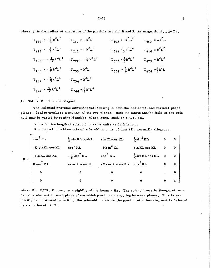
2-26 19

where p is the radius of curvature of the particle in field B and R the magnetic rigidity Bp .

T111 .! kzL z 2 T211 - k

2L T 313 =

kZLZ T 413 = Zk

2L

T112 =-.!_k2L3

3 T 212 - kZLZ

T 314 -.!kZLZ -3 T 414

= kZLZ

T122 __!_ kzL 4

Tzzz _..!_k2L3 1 2 3

T423 = kZLZ

12 3 T323 =3k L

T133 .! kzL z 2

T 324 .! kzL 4

T424 =~k2L

2 T 233 = k L 6 3

T134 - .!_k2L3 2 2

3 T 234 = k L

T144 ....!.. k2L4 1 2 3 12 T 244 = 3k L

19. NM L. B. Solenoid Magnet

The solenoid provides simultaneous focusing in both the horizontal and vertical phase

planes. It also produces a mixing of the two planes. Both the length and/or field of the sole­

noid may be varied by setting Nand/or M non-zero, such as 19.01, etc.

L = effective length of solenoid in same units as drift length.

B =magnetic field on axis of solenoid in units of unit (9), normally kilogauss.

cos2KL ~ sin KL cosKL sin KL cos KL 1 . ZKL Ksm 0 0

-K sinKL cos KL cos 2 KL -Ksin2

KL sinKLcos KL 0 0

-sinKLcosKL 1 . ZKL cos2

KL k sin KL cos KL 0 0 R

- R Sln

Ksin2

KL -sin KL cos KL -·Ksin KL cos KL cos2

KL 0 0

0 0 0 0 1 0

0 0 0 0 0 1

where K = B/ZR, R = magnetic rigidity of the beam = Bp. The solenoid may be thought of as a

focusing element in each phase plane which produces a coupling between planes. This is ex­

plicitly demonstrated by writing the solenoid matrix as the product of a focusing matrix followed

by a rotation of + KL

u u u u ~ u 4 ;:) 0 7

2-27 20

cosKL 0 sinKL 0 0 0 cosKL f<sin KL 0 0 0 0

0 cosKL 0 sinKL 0 0 -KsinKL. cosKL 0 0 0 0

-sinKL 0 cosKL 0 0 0 0 0 cosKL ~sinKL 0 0

0 -sinKL 0 cosKL 0 0 0 0 -KsinKL cosKL 0 0

0 0 0 0 1 0 0 0 0 0 1 0

0 0 0 0 0 1 0 0 0 0 0 1

20. N 8. Beam Rotation

The 20. element introduces a rotation in the X-Y plane. This rotation causes a mixing

of the horizontal and vertical plane. 8 is the angle of rotation in degrees taken as positive in

clockwise direction as one looks along the positive Z axis. If N :f 0, 8 is a variable. The

matrix representation for the 20. element is:

cos8 0 +sin 8 0 0 0

0 cos 8 0 +sin8 0 0

-sin 8 0 cos 8 0 0 0 R

0 -sin8 0 cos 8 0 0

0 0 0 0 1 0

0 0 0 0 0 1

A rotation of 90 degrees interchanges the X and Y coordinates and may thus be used to introduce

a vertical bend. The following two data sets produce identical results:

20. 90. -------2. 1. 2. 1

4. L. B. N. 4. -L. B. N.

2. 2. 2. 2.

20. -90. -------

Normally the plots produced by the 24.0. option will have the X, Y coordinates projected onto the

global coordinate system. This projecting can be turned off by use of a 13. 46. data option.

2-28

21. J. EPS. DEL. - Stray Field and Miscellaneous Input

The 21. data card is used to input various miscellaneous parameters to TRANSPORT

depending on the value of J.

J 4 Horizontal stray magnetic field

J 2 Vertical stray magnetic field

J 0 Input Betatron function phase area

J < 0 Alter interval limits on variables

21

When J > 0, the 21. data entry introduces an angular deflection in the beam of EPS/(Bp) where

EPS = s B dZ

EPS is interpreted as the mean value of the bending field and DEL as the uncertainty in this mean

value. This is implemented as a misalignment. If DEL is negative, then a angular misalignment

of DEL/Bp is introduced in the beam. If DEL~ 0, a deliberate angular misalignment of

(EPS± DEL)/Bp is introduced with the new axis used for subsequent elements.

When J = 0, EPS and DEL will be the horizontal and vertical phase space areas used with

the input of Betatron functions on the beam card. In terms of the TRANSPORT a-matrix,

EPS = .J det(a ) and DEL =.J det(a ), where a and a are the 2X2 horizontal and vertical sub-x y X y

matrices.

When J < 0, EPS and DEL will be interpreted as the lower and upper limit on the type of

variable specified by the value of J.

Element

Beam

Pole

Drift

Bend

QUAD

Align

AUX

SOL

ROT

J

-1

-2

-3

-4

-5

-6

-7

-8

-12

-13

-14

-15

-16

Variable

All beam parameters

Pole face rotation

Drift distance

Bending magnet field

Bending magnet field index

Quadrupole length

Quadrupole field strength

X, Y, Z misalignment displacemtns

XP, YP, ZP misalignment angles

All parameters

Rotation angle

These lower and upper limits are used during computer optimization of the designated variable so

as to retain physically meaningful values of the variables.

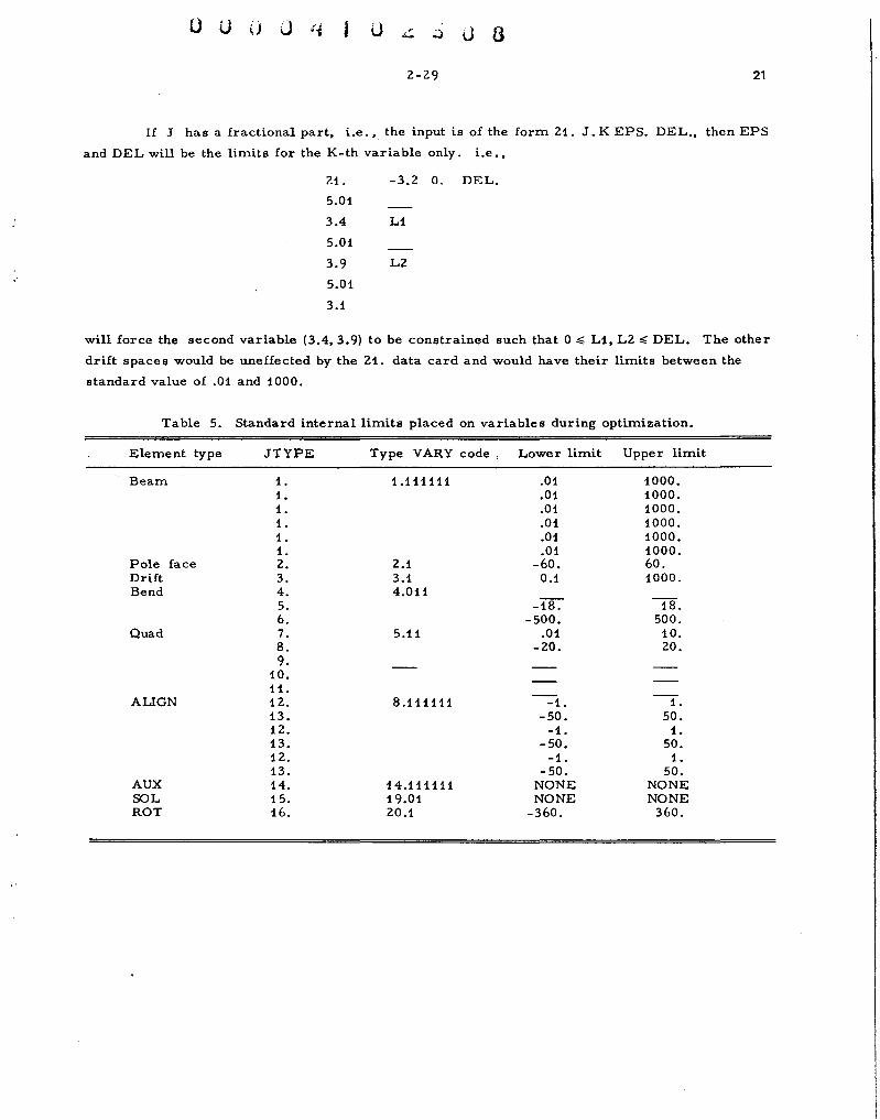
u ~ ~ J 6

2-29 21

If J has a fractional part, i.e., the input is of the form 21. J. K EPS. DEL., then EPS

and DEL will be the limits for the K-th variable only. i.e.,

21. -3.2 0. DEL.

5.01

3.4 L1

5.01

3.9 L2

5.01

3.1

will force the second variable (3.4, 3.9) to be constrained such that 0 ~ L1, L2 ~DEL. The other

drift spaces would be uneffected by the 21. data card and would have their limits between the

standard value of .01 and 1000.

Table 5. Standard internal limits placed on variables during optimization.

Element type JTYPE Type VARY code, Lower limit Upper limit

Beam 1. 1.111111 . 01 1000 • 1. . 01 1000 . 1. . 01 1000 • 1. . 01 1000 • 1. • 01 1000 • 1. . 01 1000 .

Pole face 2. 2.1 -60. 60. Drift 3. 3.1 0.1 1000. Bend 4. 4.011

5. -18. 18. 6. -500. 500.

Quad 7. 5.11 . 01 10 • 8. -20. 20. 9.

10. 11.

ALIGN 12. 8.111111 --=-1. --1.

13. -50. 50. 12. -1. 1. 13. -50. 50. 12. -1. 1. 13. -50. 50.

AUX 14. 14.111111 NONE NONE SOL 15. 19.01 NONE NONE ROT 16. 20.1 -360. 360.

2-30 22

I I

22. X.X. Y. Y. dS. dP/P. f3.-Particle Vectors

TRANSPORT can tract up to N1

first order particle vectors and up to N2

second order

vectors such that 6N1

+42N2

.:; 252. These vectors may be initiated at several points along the

beam line. Each group of vectors requires two locations in the data array and is stored in

separate arrays VI(252), VC(42). The starting coordinates of the vector in the six-dimensional I I

phase space are X, X , Y, Y , dS, and dP/P. {3 is the relativistic velocity (v/C) of the particle

and needs only be specified if the vector is to be deflected by a particle separator (type 23

code). The units of the starting coordinates are in the same units as the beam ellipsoid (type

code 1).

If {3 ~ 2, the vector is a second order vector. For {3 = 2 the second order elements

of the vector are simply the square of the first order elements. If {3 ~ 3 then the 22. data card

is followed by {3 pairs of numbers which specify the second order elements and values, e. g. I

input of XX , X o and XY second order terms as follows: I I

22. X. X. Y. Y. dS. dP/P. 3. I

12. XX . 16. Xo. 13. XY.

The vector space is symmetric in second order so that XjXk = XkXj with the appropriate sym­

metry in the R matrix. The vector input routines will automatically symmetricize the data so

that in the example, only the 12., 16., and 13. elements are to be specified.

If the first order part of the second order. vector is zero the vector plays the role of

projecting the aberration elements of the second order transformation matrix by setting the ap­

propriate second order term to unity. For example, if one wishes to follow the value of T(112),

input:

I I

22. 0. 0. o. 0. 0. o. 3.

12. 1. 0. o. 0. o.

The value of X. X • Y. Y. dS. and op. along the beam line will then be T(112), T(212), T(312),

T(412), T(512), and T(612).

If the component (8-th) entry on a vector card is negative, the card will be treated as

a vector generator card, generating a group of vectors, i.e.,

22. Fi. F2. DF. Q1. Q2. DQ. -FQR.

Where R is the random flag and F, Q specify the vector positions to be generated, I. E.,

F,Q = i(X), 2(XP), 3(Y), 4(YP), 5(dS), 6(dP/P), where

F=F1, F1+DF,

Q=Q1, Q1+00,

F1+2DF,

Q1+2DQ,

F2.

Q2.

Q takes these values for each value of F. A maximum of 42 vectors may be generated. The

total number, N, of vectors generated is

N=( (F2-F1)/DF+1) * ( (Q2-Q1)/DQ+1).

The value of the unspecified components is taken from the preceding vector card if there is

one, or otherwise set to zero. The values are chosen on the grid if R is not specified.

Otherwise they are chosed randomly within the area encompassed by the grid, E. G.,

22. o. 22. o.

I U·, <·

.-.:: ~ 0 9 2-31

o. 0. 0. o. 0.'5

1. 5 o. 25 o. 5. 1. -12.

wi 11 generate 42 vectors in the horizontal phase plane with dP/P =.5 on the specified grid of

points, whereas

22. 0 0 0 0 0 0. 5

2?. 0 1. 5 0.25 0 5 1 -121.

will generate 42 vectors randomly chosen in the horizontal phase plane with dP/P=. 5, such

that 0 ~ X ~ 1. 5, 0 ~ XP ~ 5.

22

If it is desired to know where vectors are lost, the 13 component may be used as a flag

if the 16. 14. option is specified. This will cause 13 = ± L where L = length at which vector

exceeded a horizontal aperture for L> 0 or a vertical aperture for L < O.

The transformation for a particle vector J is

V. = RV. J J

where R is the transformation matrix of the given beam element. Unlike the phase space trans­

formations, vector tracking is not updated by constraints. The particles to be tracked from the

point of. insertion to the end of the beam line. The parameters controlling the vector tracking

output are the same as the beam matrix, i.e., 13. 1., 13. 2., and 13. 3. Additionally:

A

A

A

13. 25.

13. 26.

13. 27.

card will terminate all ray tracing output.

card will permanently override a 13. 25. suppression code

card will override a 13. 25. request only at the point of occurrence.

The horizontal and vertical positions of the first six vectors will be tabulated in the 11A" table,

and will appear on the beam line graph.

The various vectors are labelled in the output by a number and a symbol as shown in

Table 6. These symbols are used to locate the vector on any phase plots designated by the plot

cards.

Table 6. Symbols corresponding to vectors used in phase space plotting.

1(A) 6(F) 11(L) 16(Q) 21(V) 26( -) 31 (=) 36( [)

2(B) 7(G) 12(M) 17(R) 22(W) 27(/) 32(,) 37(])

3(C) 8(H) 13(N) 18(S) 23(Y) 28()) 33(0) 38(±)

4(D) 9(J) 14(0) 19(T) 24(Z) 29( () 34(*) 39(-)

5(E) 10(K) 15(P) 20(U) 25( +) 30( $) 35(=) 40(<)

2-32 23

ExamEle:

Test ray tracking

0

1. 1. 2. . 35 3. 0 . o. 725.

22. 1. o. . 35 o . o. o. 22. o. 2. 0. 3. o. 0.

22. o. o. 0. o. o. 1.

22. 0. o. o. o. o. 3.

13. 25. No vector output

3.

5.

3.

5.

3.

13. 27. Vector output here

3.

22. 1. 0. • 35 0 . 0. o. 22. 0. 2. o. 3. 0. o.

4.

3.

5.

3.

5.

13. 26. Vector output

3.

l 3.

3.

73.

23 .. L .V. Ah. Av. l3o. -Particle separator

The particle separator of TRANSPORT will deflect vectors according to their 13(=v/c).

TRANSPORT follows up to 42 vectors each of which may have a different 13 and so may repre­

sent several simultaneous secondary beams of the same particle momentum.

A particle separator consists of a crossed B and E field which produces no deflection

of particles of the correct velocity 13 but deflects particles of any other velocity 13. If V is the 0

potential on the separator plates of length L separated by an aperture A, then the angular deflec-

tion produced at the entrance and exit to the particle separator is

P is the momentum of the undeflected particle. In TRANSPORT the particle vectors I I

have seven parameters: x, X • y. y • s, op/p. 13· The vector transformation for the particle

0 u u 0 .ti I 0 • .I :..> 0 c..

2-33 24

separator is then

X i L 0 0 0 0 X ·o

X 0 i 0 0 0 0 X + (} (}X X

y 0 0 i L 0 0 y 0 +

y 0 0 0 0 1 0 y + 8 (} y y

s 0 0 0 0 0 i s 0

op/p op/p 0

where (} = 0, (} = (} for vertical deflection and 8x= 8, (} = 0 for horizontal deflection. X y y

24. J.X. Y. Z. Vf. V2.- Plot OEtions

On-line paper plots and certain data input are provided by the type 24 element. The

meaning of the parameter list X, Y, Z, Vi, and V2 is selected by the value of J.

J 0 BEAMLINE PLOT

Request a plot of the beam line and apertures to be on the output paper. X and

Y are the horizontal and vertical beam plane scales and Z is the number of

drift length units per print (plot) line. If Z is zero, the plot will be adjusted

to be two pages in length. If X and/or Yare zero the scales will be set by

the data to be plotted. In addition to the beam envelope and magnet apertures,

vectors Vi, V2 may be displayed where 0 ~ V2 ~ 6, Vi ~ VZ.

The plot may be suppressed by a i3. Z.i entry.

J = 1 TARGET SIZE UNIT

Define the horizontal and vertical position of a rectangular target, (Xmin = X,

X =}? and (Y . = Z, Y = Vi). The overlap area of the target so de-max m1n max ,

fined with the beam acceptance polygon will be calculated during an aperture

calculation (i3.5. and i3.6 using option 5) to find the uniform illumination

transmission and rnillisteradian acceptance solid angle.

J = 4 ENERGY SPECTRUM

During an energy spectrum calculation under Oplion 5, the aperture polygons

of the section of beam line bracketted between a 13. 5. and 13. 7. data card

will be calculated on momentum interval between Pmin = X to Pmax =Yin

steps of dp = Z (energy interval if a 16. iS. data card is used). This card

must preceed the 13. 7. data card and would normally occur at the beginning

of the data deck.

2-34 25

J 5 SOURCE SPACE PLOT SCALES I

The horizontal polygon phase space plot scale (X, X ) will be set to (X, Y) I

and the vertical polygon phase space scale (Y, Y ) will be set to (Z, Vi).

This plot occurs for apertures transformed to the 13. 5. data card location.

In the absence of the 24. 5. ---- data card the plots will be scaled to contain

the beam phase ellipse and the polgon vertices.

J 6 IMAGE SPACE POLYGON PLOT SCALES

Same as J = 5 except now pertains to the plots at the i3. 6.or 13. 7. data card

location when these plots are activated by a 13. 30. data card.

J F PHASE SPACE BEAM PROJECTIONS

A plot of the projection of the beam ellipsoid will be generated by this option

where F specifies the phase planes to be plotted. If X and Y are non zero

they will designate the scale of the plot. If they are zero the code will find the

scale for the plot. If F < 0, the page eject following the plot will be sup­

pressed.

F = 12. F = 34. F = i3. F = 16. F = 1234i6. F = 3412.

I

XX, plot YY plot XY plot Xo , plot , (XY, ), (YY, ), (Xo) plot's (YY ), (XX ) plots on individual pages etc.

If Z and Vi are non zero they will specify a fix scale for the second of each group

of two plots, e.g., 24. 123416 •• 360 10. 2.5 i5. willplotthe i2. and 16. phase

planeonascale of .36Xi0. and the34phaseplane on a scale of 2.5X15. If V2 is non

zero the plot scales are xmin, xmax, ymin, ymax =X, Y, Z, Vi.

J = 7 PHASE PLOTS FROM A-TABLE

The 16. KLM. IJ. data cards can cause the storage of the beam or vector X, X I

I

or Y, Y phase points into the X-Y positions of the vector columns in the A-table.

These points may be plotted by giving

24. 9. VEC. Xi. X2. Yi. Y2.

where VEC is the vector number whose X- Y positions are to be plotted and

X 1, X 2, Y i and Y2 are the X- Y scale minima and maxima if given. Should

Xi= X2 = Y2 = Y2 = 0, the code will find the necessary scale.

25. MA. INTYPE. FARM. -Calculated Matrix

The 25. element will accomodate the input of first and/ or second order transfer matrices

without filling the data array. Alternatively, TRANSPORT can calculate the matrix and then

used it without the necessity of recalculation, saving much computer time in some cases. The

matrices readin or calculated and subsequently stored via the 25 element can cross from one

data case to the next provided that the momentum and units are not changed from one data

0 u u ' -· ....

2-35 25

case to the next.

On first order TRANSPORT's provision is made for up to 15 matrices to be read or

calculated and saved for use in the current data case or any subsequent data case depending on

if INTYPE is positive, negative or zero. If INTYPE is positive the matrices are readin from the

input file. If INTYPE is negative the RC, RC2, RTN or R matrices will be saved according to if

INTYPE is -1, -2, -3, or -4 respectively. In second order only the RC matrix can be saved, so

INTYPE should always be -1 or 0.

25. NAME. INTYPE. T2ND.

The matrices saved under name NAME will be used as the R-matrix whenever a data card of

the form

25. NAME. o. o.

is encountered. Since only 15 such names are allowed in first order and four such, names in

second order, provision is made to reset the matrix storage pointer via a

25. 0. 0. 0.

data entry. 15 new matrices can then be saved, or four new matrices in second order.

When INTYPE is greater than zero, a matrix will be readin from the input file. The

first order part of the matrix is readin row-wise, INTYPE/10 rows which will be stores in a

special array under the name NAME. The matrix so read will be applied as a transformation

at this point in the beam.line as well as at any location where a 25. NAME 0. 0. data card

appears. As an example, consider the input of the first four rows of a matrix (first order) with

name KRUD. The data would be:

25. KRUD. 40. o. $ INPUT 40/10 ROWS. 1.99 3.44 0 0 0 .234 $ROW 1

-2.43 -3.708 0 0 0 1.674 $ROW 2 0 0 -1.676 -.527 0 0 $ROW 3 0 0 -3.438 -1.678 0 0 $ROW 4

The length associated with this matrix can be specified bya preceding 16. 17. length card.

This matrix will be used in the calculation of the beam line at the location of the

25. KRUD 40. 0.

data card and- any location where a card of the form

25. KRUD 0. 0.

is encountered.

When INTYPE is negative, a matrix calculated by TRANSPORT is saved under the

name specified. As an example the following two data sets will produce the same matrix trans­

·- formations:

9. 4. 6. 0. 1. $ UPDATE RC MATRIX 3. 1.5 3. 1.5 4. . 75 11.6 o. 4 . . 75 11.6 o. 2. 12. 2. 12. 3. 2.0 3. 2.0 9. 0. 25. SAVE -1. $ SAVE =RC MATRIX

25. SAVE 0. $ USE SAVE 25. SAVE 0. $ USE SAVE 25. SAVE 0. $ USE SAVE

In first order cases with INTYPE =-1, the inverse matrix will be stored when T2ND =-1 or the

reflection matrix will be stored when T2ND =-2.

2-36 25

The 25. element can also be used in second order for the insertion of an arbit~ary

first and second order transfer matrix into the beam line calculations. This facilitates the

calculation of real beam lines which use numerically calculated second order matrices. 7 Up

to four diffe.rent second order matrices can be accommodated each displacing only four loca­

tions in the normal data array. These matrices are stored in separate arrays and each may

be referenced in the data array in more than one location.

The vector space used by TRANSPORT is 42 dimensional with six values specifying

the first order components

I

X = (x, X , y, y , S, op/p).

There are 36 second order components (xj xk' = 1, 6, k = 1, 6). The expansion of xi

through second order in the initial condition is

Then a

order

T. "k lJ

6 6 6

X. = I R. .x. l l J J + I I T .. kx. xk

l J J j = 1 j =1 k=1

There are only 21 unique second order T elements for each i since xj~ = ~xj.

complete matrix is specified by the 36 first order Rjk elements and the 126 second

Tijk elements . .It should be noted that (xjxk) contributes 2Tijk to xi since

Tikj"

SECOND ORDER, INTYPE = NM.

Examples:

N gives the first order matrix input information and M gives the second order

matrix input· in£ ormation; i . e. ,

The ten' s posit ion gives the number of rows of the first order transfer matrix to be

read. The units position gives the type of second order matrix input to be used.

e. g., if INTYPE =' NM., then M = 1 specifies the reading of PARM pairs of num­

bers, ( ijk, T .. k) while M = 2 specifies the reading of all 21 T. "k matrix elements lJ lJ

for the i' s given by PARM. If PARM = 12346., then the input will consist of the

21 numbers (T1jk' k = 1,6, J = 1,k), the 21 numbers (T 2jk' k = 1,6, J = 1,k) ..••.

( T 6jk' k = 1, 6, J = 1, k). If INTYPE = 0, no matrix is read, but the matrix

stored previously in array name is inserted into the calculations.

Input of first order matrix only in array 3. ______ 25. 3. 60. 0.

Input of first 4 rows of first order matrix only into array 2. ____________________________ ~-----

Six data cards follow 1 for each row

25. 2. 40. 0. Four data card follow

~nput of TaU' T 112, T_211 , and :r311 1nto secon order matrtx at locahon ----------- ~5data 1 ~arJ; foli~w

uvu I..Ji.4

2-37 25

Input of entire second order matrix co-efficients for x, x and s. (:1,2, and 5). _______ 25. 2. 2. :125.

:18 data ,cards follow 6 for X, 6 for X and 6 for dS.

Input of entire first and second order matrix into location 4 --------------~--25. 4. 62. :123456

42 data cards

Store and use first and second order matrix KRU 25. KRU. -:1. 0. $ Store 25. KRU 0. 0. $ Use

Example data

Beam line with two different arbitrary second order matrices 0 :1. 2.54 :10. 2. 54 :10. 0. o. :1.39 3. :1. 5. .75 7.4 :15. 3. :1.

:17. :1. 0. 3. 25. :1. 4:1. :10.

R:1:1. R 12• R 13 • R:14. R:1S. R 16•

R2:1. R22. R23. R24. R2s. R26.

R3:1. R32. R33. R34. R35. R36.

R4:1. R42. R43. R44. R45. R46.

:1:13. 2:1:1. 4:1:1.

T(:1:13). :1:14. T(:1:14). :1:16. T(:1:16). :123. T(:123). T(2:1:1). 236. T(236). 3:12. T(3:12). 336. T(336). T(4:1:1). 436. T(436).

3. :10. 5 •• 75 -3.5 :15. 3. :1.

25. 2. 42. :13.

R:1:1. R 12• R 13 • R 14• R:1S. R 16•

R2:1.

R3:1.

R4:1.

T(:1:1:1). T(:1:12). T(:122). T(:1:13). T(:123). T(:133). T ( :1:14). T(:124). T(:134). T(:144). T(:1:15). T(:125). T(:135). T(:145). T(:155). T(1:16). T(:126). T(:136). T(:146). T(:156).

T(3:1:1). T(3:12). T(32Z). T(3:13). T(323). T(333). T(3:14). T(324). T(334). T(344). T(3:15). T(325). T(335). T(345). T(355). T(3:16). T(326). T(336). T(346). T(356).

3. 5. :13. 4. 73.

T(:166).

T(366).

:1st 4 rows of 1st order transfer matrix

:10 pairs of 2nd order ) matrix demands

}

:1st 4 rows of :1st order matrix

1 i = :1 second order

I ·submatrix T:1jk

)

} i = 3 second order submatrix T 3jk

Exam2le of beam line with one 2nd order

0 1. 2.54 10. 2.54 10. o. 3. 1. 5. .75 7.4 15. 3. 1.5 17. 1. 0. 3. 25. 1. 42. 12.

R11. R12 .. R13. · R14.· R15.

R21.

R31.

R41.

T( 111). T(H2). T(113). T( 114). T( 115). T(116).

T( 122). T( 123). T( 124). T( 125). T( 126).

T(133). T(134). T(135). T(136).

T( 144). T( 145). T( 146).

2-38

matrix at

0. 13.9

T(155). T(156).

2 locations

T(166).

T( 211). T( 212). T( 213). T( 214). T( 215). T( 216). T(216). T(236) T( 246). T(256). T(266).

3. 7. 5. • 75 3. 2. 25. 1. 3. 4. 13 .. 4. 73.

-5. 15.

o. 0.

26. DL. AMPS. PRTFQ. RFFRE. S2ace Charge

26

INPUT of 1st and 2nd order matrices in array 1.

Repeat matrix stored in array 1. at this location.

The space charge type card will cause the type 3, 4, 5, and 19 elements (drift spaces,

bending magnets, quadrupoles and solenoids) to be divided into sub-lengths DL and any re­

mainder with a space charge impulse applied at the end of each sub-length. Either a two or

three dimensional model can be used by setting the rf frequency to zero for the two dimen­

sional model (D. C. beam) or to the beam pulse frequency for a three dimensional model (pulse

______ b~am with length given by the seventh parameter on the beam card). The data input parameters

are:

DL = distance interval at which space charge impulse will be applied

AMPS = applied current of beam in amperes

PRTFQ. =print frequency in units of DL

RFFRE = rf bunch frequency in MHz

When using space charge the mass of the beam particles must be specified via a 16. 3. SM

data entry in units of electron mass (units 10).

u u u u "i 3

Z-39 \ 27

The space charge impulse is calculated from the electric field of the elliptical charge

distribution given by the beam sigma matrix. The space charge calculation effects all trans­

formations; the beam, and vectors, and the R, RC, and RCZ transformations. The transforma­

tions are:

Rsc = 'II'R.E. J J

T u = RscuoRsc

RC = RscRC

v = Rscvo

RCZ = RSCRCZ

Here, R. is the transformation matrix for the sub-length, E. is the electric field matrix for J J .

space charge forces, and RSC is the accumulated transformation matrix for the element. \

Z7. L. V. RFPHSE. RFFREQ.- RF Buncher

The rf buncher introduces a focusing term in the horizontal and vertical phase space

from the rf field ·and a dependence of momentum spread on longitudinal position within the bunch.

The energy spread in the bunch is assumed linear. The transformation matrix for the rf buncher ·

i!' given below.

L = Length of buncher, must be zero

v = rf voltage in mega-volt' s

RFPHASE = rf phase, must be either 0 or 180 degrees

RFFREQ = rf frequency in mega-Herzt.

t 0 0 0 0 0

_>-;zi t 0 0 0 0

0 0 1 0 0 0 R =

0 0 _>-;zi 1 0 0

0 0 0 0 1 0

0 0 0 0 'A. 1

where

--J,• ,;"' '· •• .,.

2-40

Z1rcos (RFPHASE). V. RFFREQ

a. • sm · 'I · (3 3

e a. =--3 = 15350.0

me e

(3 =relativistic velocity, V/c

SM = n1ass of particle in units of electron mass.

27

/

3-1

Section 3 - Modification of Data

'OPTIONS

The first data card in every TRANSPORT data case is a title card and the second data

card in every TRANSPORT data case is an option card that specifies the type of deck that fol­

lows. If the first option is greater than 0 in _a given data case, then more than one option card

may appear in that data case with the case always ending in an Option 0. Remember that an

Option 0 ends with a 73. data card as the last card in the data case. Consider a data deck in

which.the Option 0 data has already been processed and the next case is as follows:

Example 1 1. X. XP. Y •.•••• 22. X. XP. Y ..•••• 2 37. -10. 44. -10.

0 73.

Title card Option card Beam card Vector Option card Option 2 data Option 2 data Option card {may be blank) Option 0 terminator.

The Option 0 data which comprises the basic TRANSPORT data deck has already been ex­

tensively discussed. I will now examine the options that modify this basic data.

OPTION 1 Data Input

Option 1 allows the input of new particle data to be transformed_ by the existing beam line.

Option 1 only allows beam data (type 1), axis shift data {type 7) beamcorrelationdata {type 12) and par­

ticle vector data {type 22) input, The data replaces the 1, 7, 12, or 22 data in the original data deck and

the run is repeated if Option 1 is terminated by Option 0 {see Examples 1 and 2 below), If the option is

terminated in a second order TRANSPORT by Option 4 the data will be transformed to the end of

the beam line by the existing RC matrix and a phase plot produced if a phase plot card ( 24.

123416., etc.) existed in the original data deck (see Example 3 below).

Example 1, Option 1, 0

1 1. X. XP. Y. YP. S. DP. P.

22. X. XP. Y. YP. S. DP. C. 0

73.

Example 2, Option 1, 2, 0 1 1. X. XP. Y. YP. S. DP. P.

12. XXP. 0. 0. 0. 0. YYP. 0. 0. o. sx. 0. o. 0. 0. o.

22. X. XP. Y. YP. S. DP. C. 2

143. -10. 0

73.

3-2

Example 3, Option 1, 4, 0 1 1. X. XP. Y. YP. s. DP. P.

22. X. XP. Y. YP. s. DP. c. 4 0

73.

A beam line may be continued via the Option 1 with a negative beam card. This will

cause the beam card, correlation card and vectors if present in the data array to be updated

with the terminal values from the .previous case. When execution is then attempted, the vectors

and beam will be continued without being re-initialized so that the beam line is continued from

the previous case. Consider running ZOO revolutions in an accelerator whose single-turn ma­

trix has previously been calculated and stored under the name FULLT.

RUN TURNS 1 - 100 0

16. 16. 1.

22. 12. 17.

216 11 $ STORE VECTOR 1 X as VEC 2-X 236 22 $ STORE VECTOR 1 XP as VEC 2- Y 1. 3.3 .7 6.4 0. o. 5.

9. 25. 13.

1. 0. 0. o. o. 0. z. ORiS 1. o. 3. 100.

FULLT 0. 0. 1. 0. 9.

24. 73.

7. Z. $ phase plot VEC 2, i.e., VEC 1 X-XP

RUN TURNS 101-200 1

- 1 $ Beam card with type code = 0

73.

-1., continues beam.

The division into two runs of 100 TURNS each is necessary because the A-table can accommodate

only 99 entries. Note that no harm is done by overflowing the table as in the previous example;

100 turns will lose the plot and table entry number 100 and 200.

OPTION 2

Option 2 allows the alteration of the data as left by the preceding data deck. Changes of

a single data element may be made by reading the value of the index counter of the data to be

changed followed by the chance, or by using special control cards such as

ALTER - ·Alter one or more data elements. ALINE - Add a line to the data. DLINE Delete a line from the data. FIX - Fix the variable and remove the constraints. MOVE - Move one or more data lines. NAME - Re-name the data. PUNCH - Write the data array out on tape 7. REVERSE - Reverse data order in array. REFLECT - Change sign of vector X and Y

1•

BETAF - Betatron Function generator.

The reading of these cards and the modification they produce to the data deck continues until a new

option card is encountered. This causes initiation of the new option. Finally, the data case is

terminated by a blank card (option= 0) and resumption of standard {option 0) data input occurs.

3-3

lnorder to better understand how the Option 2 control cards operate on the data, I will

describe the naming procedure for the data array and then give a detailed account of the use of

Option 2 control cards.

Data Array and Names

The data appearing between the option card and the sentinel card (or 73. card) serially

fills a singly dimensioned data array, with each number specified,_located in the data array at

position given by the data ·array counter, I. . The data may subsequently be altered by reference

to it by its I count value. Alternatively, each data input card may be given a name (if not ex­

plicitly by the user, the code will generate a unique name for each data card) which then can be

used to alter or refer to the various parameters of that line in the data array. The names are

restricted to six or less alphameric characters, the first of which must be alphabetic.

For each name there corresponds an I, the I of the type code. The data is stored in the

data array in the order the cards are read in consequently the names are in that order also. In

this report, we will often refer to name pair's (e. g., NAME 1, NAME 2) where NAME 1-must re­

fer to a smaller or equal I count than NAME 2, that is, the data line for NAME 1 preceeds the

data line for NAME 2 or NAME 1 equals NAME 2. We will also often refer to index pairs (e. g.,

11, I2) where 11 must be less than or equal to I2. Names and I counts may be mixed, i.e.,

NAME 1, NAME 2 could be replaced by NAME 1, I 2 where I 2 is the index counter value of NAME 2.

More than one data line. may have the same name. The advantage of this is that all

these cards can be changed, deleted, etc., together by the ALTER, ALINE and DLINE operations,

referencing that respective name.

The standard name generation of TRANSPORT is shown below. The names will be gen­

erated by the type of data element and an incremental counter appended, i.e., 01, Q2, Q3, etc.

for quadrupoles, name Q. These names will be unique and may be used with the ALINE, ALTER,

DLINE and MOVE operations.

Standard name

BEAM FF L BM Q SLIT AXIS ALIN REP CON ACC TIL IO AUX UNIT DA SEC SEX roL STRY

Type

1.000000 2. 0 3.0 4.000 5.00 6. 7. 8.000000 9. 10.0 11. 12. 13. 14.000000 15. 16. 17. 18. 19.00 21.

Meaning of Card

BEAM CARDS FRINGING FIELD TO BENDING MAGNET DRIFT SPACE BENDING MAGNET QUADRUPOLE SLITS AXIS CARDS ALIGNMENTS CARDS REPEAT CARDS CONSTRAINT CARDS ACCELERATOR CARD PHASE SPACE TILTS INPUT- OUTPUT CARDS AUXILIARY MATRIX UNIT CHANGE CARD PARAMETER CARD SECOND ORDER SEXTUPOLE SOLENOID STRAY FIELD

VEC SEP PLOT MAT sc BUN

22. 23. 24. 25. 26. 27.

3-4

VECTORS PARTICLE SEPARATOR PLOT CARD MATRIX INPUT CARD SPACE CHARGE BUNCHER

Names and Duplicate Names. If two or more data lines have identical names, they

will be altered or deleted together. The ALINE option used with a duplicate name data will

insert the new line after each appearance of the name in the data deck. To alter the J -th

position of the N-th multiple named data ·line requires the input of N and J after the name,

i.e. •

ALTER, NAME, N, J. CHANGE.

To add the new line after the N-th occurrence of the multipally named data only, N

must be specified after the name, e. g., to add a 13. L line after the second QUADH data

line, one would use

ALINE, QUADH, 2, 13. 1.

If only the N-th multiply name line is to be deleted, N follows the Name, e.g., to delete

the second quadrupole QUADH one would enter

DLINE, QUADH, 2

It is not possible to use. a multiply-named data· element as one parameter of a multiple delete,

i.e., the following card is illegal:

DLINE, QUADH, I03,

if either QUADH or I03 are multy named data.

ALINE orAL. The ALINE (add line) c:>ption allows the user to add new data lines and

elements to his data array during Option 2. The entries consist of the location or name of the

line after which the new line is to be added, followed by the new line. Example: consider

adding a 13. 1. data line after a drift with name DRFT 4 which occurs with an index value of

29 in the date array. This can be accomplished by one of the following entries:

ALINE, 29, 13. 1. ALINE, 29, 13. 1. NAMEX ALINE, DRFT 4, 13. i. ALINE, DRFT 4, 13. 1. NAMEX

If the name NAMEX of the new data line is not entered, the code will generate a unique name

for the new data line.

ALTER or A. The ALTER option allows the user to change or alter any element in his data

array. There are two general schemes that can be employed, one uses the location of the el­

ement to be changed by designation of the storage index I, within the data array, the other uses

the unique name of the data line and the location of the element to be changed within this line.

Example, consider changing the field strength of the first quadrupole with name QV to -8. 75 KG.

This quadrupole occupies, say, location 19 through 22 in the data array and has name Q V. The

alteration can be accomplished by any of the equivalent entries.

v v u u '"1 6

The general scheme is

3-5

ALTER, 21, -8.75 ALTER, QV, 3, -8.75 ALTER, QV, 1, 3, -8.75

ALTER, NAME, N, J, CHANGE.

where NAME is the name of the data line, N would only be needed if more than one data line

has this name. J is the position on this line for the change. If more than one consecutive

change is to be made on this data line, these changes may be entered together. Consider

changing the length and field of a quadrupole QV to 0. 75M and -13.65 kG; the entry could be

ALTER, QV, 2, 0. 75, -13.65

DLINE. or D. The DLINE (delete line) option allows the user to remove a data line from

his data array. A group of lines may be removed together by specifying the name or index of

the first line and the last line, bracketing all lines to be removed.

DLINE, I DLINE, NAME DLINE, I 1, I 2 DLINE, NAME 1, NAME 2 DLINE, NAME1, Ni, NAME2, N2 ETC.

FIX. The FIX option removes variables· in .the data array .by zeroing the vary. c.odes (

of each type code and. negating:all.constraints. The fix option will operate ·on.the·entire· data

set if no delimiters are given,· otherwise it will operate from NAME 1 to· NAME 2 only.

FIX, NAME1, NAME2 FIX

The fix option operating on the data shown in column 1 produces the result shown in column 2.

It operates on all the data in the data array.

1. 1.

5.02 5.

3. 3.

5.01 5.

3. 3.

10.1 -10.1

10.2 -10.2

3. 3.

10. -10.

NAME. The NAME option allows the user to rename his data array with the standard

name convention internally generated by the code. The entry would be,

NAME.

If only one name is to be changed it may be done by entering

NAME, NAME, NEWNAME.

' I

3-6

If a string of names are to be changed, then the string is entered, ending in the new

name for the string, e. g., if L1, LS, L6, L22, and the 2nd occurrence of the multipally named

drift LL are to be given the name LX, the entry would be

NAME, L1, LL, 2, LS, L6, L22, LX

Should one wish to assign unique names to several multi-named data elements. He enters the

list of _NEWNAMES, and/or occurrence number ending the list with the old name followed by

an *· For example, say one wished to change the 1st, 2nd, 5th, 6th, and 22nd occurrence of

the data named LX to LD1, LD2, LDS, LD6, and ID22, then the entry would be

NAME, LD1, LD2, 5, l.DS, LD6, 22, LD22, LX * MOVE. This option allows the user to move a group of data. within the data array

MOVE, NAME 1, NAME 2, NAME 3.

Here the data lines NAME 1 to NAME 2 are moved to follow NAME 3. If only one data line is to

be moved the entry would be

MOVE, NAME1, NAME3.

POLYGON. The POLYGON entry in Option 2 will set OPTION=POLYGON and initiate

the polygon calculation as explained elsewhere.

PUNCH-PUNCH, X-PUNCH, COMMENTS FIELD. The PUNCH card included in the

Option 2 deck will cause the data array to be written to tape 7 in field free format with data

names appended. If there is a second non-blank entry on the punch card, tape 7 will be written

in 8F10. Format without names. In either case the data on tape 7 may be used as input to trans­

port on subsequent runs. If a third entry is made on the punch card, the entry will generate a

comment card which will precede the title card of the data case punched. e. g. PUNCH,, this

comment will precede the title card. The comment will automatically start with a $ so as to be

properly read by the field free input routine of TRANSPORT.

REVERSE, NAME 1, NAME 2. The REVERSE option allows the user to reverse the

data entries from NAME 1 to NAME 2. This is particularly useful when wanting to run the beam

backwards or to make a symmetric data case with the pull option. The effect of entry of re­

verse Q1, Q2 will be the following:

Original data

1R8 3 1. 25 5 . 56.2 4 Q1 3. 5 L2 5 . 5 -3.6 4 Q2 3 1. 75 L3

13 4 SENTINEL

Effect of Reverse

1R8 3.125 5 • 5 -3.6 4 Q2 3 .5 L2 5 • 5 6. 2 4 Q1 3 1. 75 L3

13 4 SENTINEL

Comments

First data card Second data card Note Q2 is first

Note Q1 is last

END CASE

Some care must be used if the order of the data is important when using the reverse procedure.

For example, the apertures of the bending magnets must precede the bending magnet card.

Consider the following example of a quadrupole doublet constrained to produce first a

focus and then a waist. After solving for the waist the beam line is continued by adding a bending

UUi.JU·'~

3-7

magnet and a new quadrupole.

BEAM FOCUS

0 1. 3. 5.01:..__ __ _

3. ,.-:-----5.01::...._ __ _

-------I count for 5. 01 is 11

-------I count for 5. 01 is 17

l

3. -....,.---..,.-----,--10. -1. 2. 0 .. 001 ____ -:I count for -1. is 24 and 25 for 2. 10. -3. 4. 0 .. 001 I count for -3. is 29 and 30 for 4. 73. Beam waist 2 .

24. 2. 25. 1. ALTER, CON2, 2, 4, 3 --------------------------Blank card 73. Add rest of beam line 2 FIX --------------------------Blank card 3. 4.-----3. 5.01:.._ __ _ 5.01:.._ __ _ 3. 10. ____ _ 10. ____ _ 73. ____ _

REFLECT. When one wishes to run his beam line backwards, the signs of the vector divergences I I I I

must be changed. The REFLECT option accomplishes this, taking x = - x and y = - y

BETAF. The betatron function at the end of a lattice supper period can be calculated by entry of

a card under Option 2 of the form

BETAF N

where the betatron functions will be calculated from the RC matrix if N=i, the RCZ matrix if N=2

or the R3 matrix if N=3. The beam card data will be automatically replaced by

1. 13x o. 13y o.

13x = M1Z ;J 1 - M11 2

13y M34/J 1 - M33 2

a a = o. X y

The off-energy function will also be calculated if an axis shift data card follows the beam

card. In this case, the beam centroid play the part of the dispersion function with the values set

as

3-8

7. I

T) T) 0 0 0 1.

where

I T) = 0,

An output table will be generated giving the values of

a. • X

I

TJx ' 13 y' y y' a.y' flx'

Also, the transition gamma will be calculated.

OPTION 3 Data Input

and f1 • y

The TRANSPORT option 3 provides the user with the ability to cycle from one to four

data elements over a range of values. If variables are present in the Option 0 data·deck and are

not being cycled, they will be restored to their original value at the start of each run.

The total number, N, of transport runs that will be generated· by the Option 3 data is

where

N. = (V 2 - V 1)/DV. + i J j j J

J = 1,2,3,4

and NOPTIM i~ the number of Sll;bsequent runs at optimum starting values. The variables J are

cycled between v.1

and v. 2 in steps of DV.. Care must be exercised not to specify bV to small J J J

for the number of runs generated will become exceedingly large. Furthermore, in order tore-

duce execution time it is recommended that only essential data cards be present in the Option 0

data that the Option 3 data is working on,

The data input for TRANSPORT consists of a series of data decks beginning with a title

card, option card, and ending with a 73 card-the data between the option card and the 73 card is

chosen from various possible elements which describe the beam line. This data serially fills a

singly dimensioned data array, with each number specified, located in the data array at position

given by the I counter. If a user wishes to change a data element, he must specify the value of

0 u 0 u u . .­._

3-9

8

the I counter (i.e., location of data) for the element in the data array. If the data deck has been

previously run, TRANSPORT gives the I of the type code specifying the data element as normal

output. The Option 3 data operates on the data in the data array as established by the preceding

data deck or decks, and consists of a series of one or more cards specifying up to eight param­

eters per card whose meaning will now be explained.

Title card typical data deck:

3

K.J Vi. V2. DV.

. •

73.

K>O

K< 0, J = O(e. g. -21. 0)

K<O,J =i(e.g.-2Li)

K< 0, J = 2(e. g. -21. 2)

RANDOM. NOPTIM. V6. V7

MAXIMUM of 4 such cards •

K specifies which variable is to be cycled i.e., K = i means first variable, K = 2 means second variable, etc. If Ran­dom=O the variable will be assigned values between Vi and V2 in steps DV. If RANDOM f: 0 the variable will be as­signed a total of DV values scaled to lie between Vi and V2. The random number generator is started at a point deter­mined by the value of random. NOPTIM specifies how many subsequent optimization runs shall be made using the NOP­TIM best starting conditions found (smallest RMS deviation). the largest of the NOPTIM less than ii encountered in each data set will be used. V6 and·V7 are not used when K > 0.

K specifies the I of the data in the data array where I =-K. The rest of the data is the same as above for K> 0 where the parameter Data(!) is assigned values Vi to V2 in steps of DV or assigned DV random values between Vi and V2.

Each data element with J =i will be assigned values together so that a total number of (V2-Vi)/dV+1. cases will be gen­erated even though more than one data element is being changed. This type of option will move two quadrupoles along a given line in the variable space as opposed to a grid of values.

Each data element with J = 2 will be assigned the values specified on the remainder of the card until no more non­zero values are found, i.e.; data element K will assume values Vi, V2, dV, RANDOM ... V7 until subsequent data fields on the card are all zero.

If the data being cycled is accompanied by NOPTIM f 0 the output will consist of a single

line giving the RMS deviation for the fit to the constrained quantities, the value of the variables

used, and the actual value of the constrained parameters for each set of values chosen. No

optimization is performed. After completion of the cycling of the data, NOPTIM optimization

runs will be performed using the values of the variable giving the NOPTIM smallest RMS devia­

tions as starting conditions in order to obtain optimum fits. If NOPTIM=O normal transport out­

put is obtained for each set of cycled variables including optimization if appropriate.

3-10

When using Option 3, the first entry on a card may also be a data name. In this case,

the second entry will be the location of that named line for which the data applies. The third and

subsequent entries are the same as previously described. In the J = 1 or J = 2 type entries

are to be made, J is appended to the location. For example, consider a quadrupole by the

mime QQ whose field (third entry on quadrupole card) is to be assigned the 4 values given on

the Option 3 card (J = 2).

QQ 3.2 -10.27 -11.65 -12.076 -14.3.

The second number is LOC. J while entries 3-6 are the field values. If the named data is multi­

named, i.e., more than one data line has that name, it is mandatory that the occurenc·e number

follow the name. The location entry and Option 3 parameters being displaced to positions 3,

4 • • • etc. Consider cycling the length of drift for the 6-th data line by the name lSEP over the

values 2.6 to 10.6 in steps of 1. The entry would be

lSEP 6 2.0 2.6 10.6 1. 0. 4.

The general scheme used is

LOC.J NAME

NAME OCCURRENCE LOC.J

Vi VZ. DV. RANDOM. NOPTIM. V6. V7.

V1. V2. DV. RANDOM. NOPTIM. V6. V7.

where OCCURRENCE is the mandatory multi-named occurrence number.

Examples

Several examples are in order. All examples will operate on the basic data deck given

in Example 1 consisting of a bending Iru!-gnet followed by a quadrupole doublet. We attempt to

discover the quadrupole fields required to produce waist to waist transformations .. Example 2

shows the data required to cycle the two quadrupoles over a uniform grid of values shown in Fig.

7. The Example 3 data would produce a random selection of quadrupole fields in one octant of

the grid.

Often a person wishes to examine the effect on a beam line when two or more elements

move in a correlated way. Thus consider Fig. 7 where the two quadrupoles are to have equal

values but opposite polarity. Example 4, will step both quadrupoles along· a diagonal line within

this grid. A set of data elem€m~s may be assigned specific values as in Example 5. Here the

data deck of example one is modified by fixing the first .quadrupole doublet (5.01 .... 5.0 for data

elements 20 and 26) and removing the constraints for this doublet (10-+ -10 for data elements 32

and 37). To this modified deck is then added a quadrupole triplet and a new double waist con­

straint. This data deck is then acted upon by the Option 3 deck following it which cycles the

triplet over one octant for each of the quadrupole doublet field values found previously giving

waist-waist transformations.

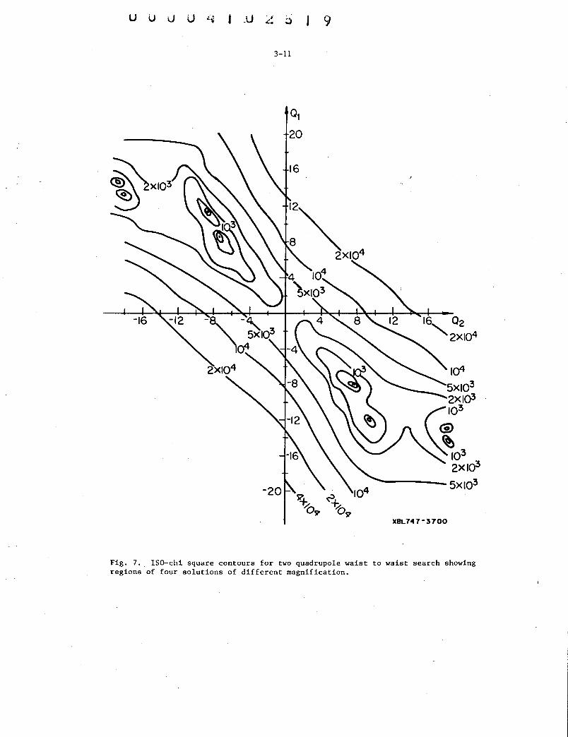
3-11

a, 20

16

9

IQ4

XBL747-3700

Fig. 7 •. ISD-chi square contours for two quadrupole waist to waist search showing regions of four solutions of different magnification.

3-12

EXAMPLE 1:

July 14, 1970 _/

1. UNIT CHANGE 0 15. 4. 15. 1. IN 2.54 15. 2. MR 1. 15. 6. PC 1. 15. 8. IN .0254 73 BASIC DATA DEK (BM/QUAD/QUAD/DOUBLE WAIST)

0 1. . 3 8. . 3 8 . 0. o. 1.3 13. 2. 4. 15. 1. 48 0.

/

2. 2.75 0. 3 138.5 5.01 16. -10. 4. 3. 8. 5.01 16. -10. 4. 3. 48. 10. 2. 1. 0. .01 10. 4. 3. 0. • 01 -10. -1. 2. o. • 001 -10. -3. 4. 0. .001 13. i. 13. 4. 73.

EXAMPLE 2:

OPTION 3 WAIST, EXAMPLE 1 3 1. -20. 0. 2. o. 4. 2. o. 20. 2. 0. Blank 73.

OPT! ON WAIST 3 1. 0. 20. 1. o. 10. 2. -20. o. 1. Blank 73.

EXAMPLE 3:

RANDOM NUMBERS, EXAMPLE 2 3 1. -20. o. 11. 1. 4. 2. 0. 20. 11. 1. Blank 73.

EXAMPLE 4:

3 -22.1 0 -20. -2. 0. 4. -28.1 0. 20. 2. Blank 73.

0 0 u 0

3-13

EXAMPLE 5:

MODIFY BASIC DATA DECK BY ADDING TRIPLET AND FIXING FIRST QUAD 2 20. 26. 32. 37. Blank car.d 3. 5.02 3. 5.01 3. 5.02 3. 10. 10. 13. 13. 73.

5. 5. ~10. -10.

48. 16. 5. 4. 8. 32. -5. 4. 8. 16. 5. 4. 64. 2. i. 0. .01 4. 3. 0. . 01 i. 4.

SEARCH TRIPLET AT EACH OF 4 MAGNIFICATIONS FOUND FOR FIRST QUADRUPOLE

3 i. 2. -22.2 -28.2 Blank 73.

SEARCH

1 3

11 13 20 22 28 30 33 37

. 40 42 44 48 50 54 56 61 66 73 78 83 85 90 95 97

o. -20. -8.38 7.26

13.000000 i. 010100

22.000000 24.000000 3.000000 5.000000 3.000000 2.000000 4.000000 2.000000

13.000000 3.000000 5.010000 3.000000 5.010000 3.000000

10.000000 10.000000 23.000000 10.000000 10.000000

3.000000 10.000000 10.000000 13.000000 13.000000

20. o. -ii.85 8.69

5. 5. -13.43 13.25

0.

-14.41 18.62

-2.000000. .200000 11.000000

8.000000 o. 10.000000 2.000000

30.000000 10.670000 8.100000 5.000000 -0.

44.130000 11.447000 40.000000 -0 . 1.000000

17.770000 20.000000 -3.251914

7.000000 30.000000 6.494160 27.050000 1.000000 1.000000 3.000000 3.000000

-120.000000 . 560000 1.000000 1.000000 3.000000 3.000000

22.550000 -3.000000 4.000000 -i. 000000 2.000000

4.000000 1.000000

5.

.100000 -13.000000

10.000000 0.

6.000000

-0.

4.000000

6.000000

5.000000 .050000 1.800000 .018000 6.000000 2.000000 5.000000 .050000 1.800000 .018000

0. ~

.001000 0. .001000

3-14

OPTION 4

Option 4 is available on second order TRANSPORT and transforms the vectors and

beam existing in the data array using the last value of the accumulated transformation matrix,

RC. The usefulness of Option 4 is apparent during second order runs where many vectors are

to be transformed in order to investigate the second order nonlinearities of the beam line. Use

of the Option 4 results in considerable saving of output and computer time since the transforma­

tion is

V. = I: RC Vk J k jk

u = RCu RC 0

with the results given numerically and plotted if a phase plot request existed in the original

Option 0 data deck, see the following example.

Second order

0 1.

22. 17.

24. 123416. 73. Track Vectors 1

22. 22.----22.----

4 0

73.

Special input cards can be used with Option 4 on second order TRANSPORT to generate

large numbers of points in multi-dimensional phase space and transform these points with the

RC-matrix. The transformed points may then be plotted in various histograms and scatter plots.

These special input cards for use with Option 4 are;

ADD CLEAR ELLIPSE

MATRIX PRINT PUNCH RANDOM,N 14 ..... . 22 ..... . 24 ..... .

Next vectors will be added End add option Grid of vector generator will have elliptical boundary. Initialize matrix to unit matrix Print vectors as they are generated Punch matrix and vectors on tape 7 Specifies how many random variables are to be used. First order matrix input Vector generator Plot

0 0" d 0

3-15

Generation of points in the multidimensional vector space is conventiently accomplished

b>' use of the vector generator card. Its general format- is

22. A1. A2. DA.. B1. B2. DB. - ABCDER.

C1. C2. DC. D1. D2. DD. E1. E2. DE.

Where A, B, C, D and E are associated with the TRANSPORT coordinates X, XP, Y, YP, and dP/P

according to the numeric value as signed to the tag -ABCDE. i corresponds to X, 2 to XP, 3 toY,

4 to YP and 6 to dP/P, so that if A, B, C, D, and E are to be interpreted as Y, YP, X, XP anddP/P,

then the tag -ABCDE would be -34126-:

The values assigned to each variable is then taken on the regular interval

aJ+i=aJ+DA; J=1, A2-A1

DA

R is the random flag. If R = 0 the flag is off and the values of the parameters are

stepped on a regular grid, If R = 1, 2, .•. 9 the random flag is on, If the random flag is on, the

number of values generated is the same as if the values were on the given grid, but the values

are chosen randomly.

The number of values produced for the first variable A is NA. Then NA = (A2-A1)/DA+1

and the total number of vectors generated for a two-dimensional space is NA*NB. The maximum

number of vectors allowed is 1024.

A two-dimensional vector generation requires only one data card. Therefore, to. step

over a grid of values in the X - XP plane, the generator card would have its eighth entry as -120.

22. A1. A2. DA. B1. B2. DB. -ABR.

Often one wishes only to randomize certain dimensions while stepping the others on a

regular grid. This may be accomplishedby the 11RANDOM, N11 entry, where N is the number of

vector dimensions to be randomized. These must be the first dimension and the vector generating

card, e. g.,

RANDOM 2

22 A1 A2 DA B1 B2 DB -36241

C1 C2 DC D1 D2 DD

Will cause Y and dP/P to be chosen randomly, while XP and YP will be taken on a regular grid.

The vectors so generated can be projected on various· coordinates creating histograms

or scatter plots. The plot card has the following format:

24 JK Si S2 S3 S4 BIN Xi X2 XP1 XP2 Y1 Y2 YP1 YP2 DP1 DP2

Plots can be one or two dimensional as specified by the JK value. The value of J and K

is related to the desired planes in the same way as the vectors are related, i.e.,

J, K= 1(X), 2(XP), 3(Y), 4(YP), 6(dP/P).

3-16

The scales of the plots can be specified by the 3rd through the 6th entry on the plot card.

S1, S2, S3, and S4 are the specified scales of the plots. If the scales are zero, then the code

will determine the scales so as to fit all the points on the plot. Histograms are produced if only

J is entered. The maximum number of vectors that can be histogramed is 1024. 'Fo plot the X

plane histogram enter 24. 1. For example: Two dimensional scatter-plots are specified by

entry of both J and K, i.e., an X- Y plot is produced by entry of 24. 13. etc. Currently, the

maximum number of vectors that can be scatter-plotted is 882. The 7th entry is not used in the

2-D plots. The number of bins in the histogram is entered as the 7th entry or the default value

of 100 is taken. 1£ non-equal entries are made for the 8, 9th 10, 11th 12, 13th 14, 15th and 16,

17th entries, then only vectors whose values in the given parameter lie between these limits will

be plotted on the scatter plots or histograms.

The first four rows of the first order transformation matrix can be inputed by use of the

14. data cards. Four such cards are required, one for each row.

14. R11 R12 R13 R14 R15 R16

14. R21 R22 R23 R24 R25 R26

14. R31 R32 R33 R34 R35 R36

14. R41 R42 R43 R44 R45 R46

Such input will clear all second order terms.

Vectors may be accumulated so that plots will show previous vectors plus those added

by subsequent vector generations. This is accomplished by the "ADD" card. To· turn off the

add option one enters a "CLEAR" card.

If one wants to plot the initial vectors, the RC transformation matrix must be set to

a unit matrix so that the subsequent vector transformations will yield the initial vectors gen­

erated. This can be accomplished by the "MATRIX" card.

The vectors generated and transformed will not normally be printed as output. The

printing can be initiated by entry of a "PRINT" card.

The transformed vectors can be written to tape 7 by entry of a "PUNCH" card. This

will cause the following to be written to tape 7:

Date and case number

Title card

First order transfer matrix 6 cards in format

Number of vector cards, NV to follow

NV cards giving the transformed N.X.XP. Y. YP.dP/P

(1H1, 7A10, A9)

(1X, 7A10)

(7X6E12. 4)

(1XI4)

(1Xl4, 3X5E14. 6)

SOLVE BEAMLINE SYSTEM

0

5. Oi 1. 2. 4.

iO 2 i 0 • OOi

73.

FIX SYSTEM, CALC RC MATRIX

2

FIX

0

73

PLOT VECTORS

4

22 OR5 2. 5 0

. 22 0 i .i 0 i7 .2 -i29.

24 12

24 i

0

73 73

3-i7

EXAMPLE

$ OPTION 0 DATA INPUT

$ VARIABLE

$ CONSTRAINT CARD, UPDATES RC MATRIX

$ OPTION 0 CASE TERMINATOR

$ NEXT CASE TITLE CARD

$ OPTION 2 DATA INPUT

$ FIXES THE DATA

$OPTION 0

$ TERMINATOR, CALCULATE RC-MATRIX

$ TITLE CARD NEXT CASE

$ OPTION 4 DATA INPUT

$ SET DP/P TO 2. 5 PERCENT

$ GENERATE 946 RANDOM VECTORS

$ SCATTER PLOT X -XP PHASE PLANE

$ HISTOGRAM X -PLANE

$ END OPTION 4

$ END JOB

The generation of the multidimensional vector space can be forced to occur inside a

multidimensional elliptical boundary by use of the ELLIPSE option instead of the 22. vector gen­

erator. The input is

ELLIPSE, Vi. V2. V3. V4. VS. N. -ABCDER.

where Vi, V2, •••• V5 will be the elliptical semiaxis associated with coordinates X, XP, Y,

YP or dP/P according to the numeric value assigned to the tag -ABCDE (A, B, C, D, E = i(X),

2(XP), 3(Y), 4(YP), 6(dP/P)). N is the number of vectors to be generated within this elliptical

boundary. R is the random flag, with the vectors generated on a uniform grid if R = 0 or

chosen randomly if R ::/ 0. Note that the ELLIPSE option necessarily operates a vector distri­

bution whose centroid is centered on the pariaxial trajectory.

3-18

OPTION 5

Option 5 will produce a polygon calculation provided the appropriate cards have previ­

ously been inserted into the basic data deck. The required cards are the 13. 5. and either a

13. 6. or 13. 7. data card as previously described. As an example, consider solving a beam

line, fixing the variables and constraints, adding a downstream spectrometer, and calculating

the polygon. The data deck structure would be:

Basic data deck

0 1. ___ _

13. 5.

5.01 ___ _

5.01 ___ _

10. ___ _

73.

$ point of origin for polygon

Fix system and add spectrometer

Fix

0

3.

4.

3.

13. 6.

73.

Calculate polygon

5

73.

$ end point of polygon calculation

$ end option 0 input

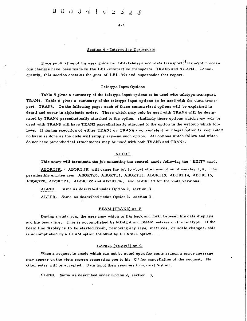
0 0 d 0 ··~ u -.J ~> •j .,

...... #1..• " 4-1

Section 4 -Interactive Transports

Since publication of the user guide for LBL teletype and vista transport?>LBL-951 numer­

ous changes have been made to the LBL-interactive transports, TRAN3 and TRAN4. Conse­

quently, this section contains the guts of LBL-951 and supersedes that report.

Teletype Input Options

Table 5 gives a summary of the teletype input options to be used with teletype transport,

TRAN4. Table 6 gives a summary of the teletype input options to be used with the vista trans­

port, TRAN3. On the following pages each of these summarized options will be explained in

detail and occur in alphabetic order. Those which may only be used with TRAN4 will be desig­

nated by TRAN4 parenthetically attached to the option, similarly those options which may only be

used with TRAN3 will have TRAN3 parenthetically attached to the option in the writeup which fol­

lows. If during execution of either TRAN3 or TRAN4 a non-existent or illegal option is requested

no harm is done as the code will simply say-no such option. All options which follow and which

do not have parenthetical attachments may be used with both TRAN3 and TRAN4.

ABORT

This entry will terminate the job executing the control cards following the •iEXIT" card.

ABORTJK. ABORT JK will cause the job to abort after execution of overlay J ,K. The

permissible entries are: ABORT10, ABORTU, ABORT12, ABORT13, ABORT14, ABORT15,

ABORT20, ABORT21, ABORT22 and ABORT 16, and ABORT17 for the vista versions.

ALINE. Same as described under Option 2, section 3 .

ALTER. Same as described under Option 2, section 3.

BEAM (TRAN3) or B

During a vista run, the user may which to flip back and forth between his data displays

and his beam line. This is accomplished by MDATA and BEAM entries on the teletype. If the

beam line display is to be started fresh, removing any rays, matrices, or scale changes, this

is accomplished by a BEAM option followed by a CANCL option.

CANCL (TRAN3) or C

When a request is made which can not be acted upon for some reason a error message

may appear on the vista screen requesting you to hit "C" for cancellation of the request. No

other entry will be accepted. Data input then resumes in normal fashion.

DLINE. Same as described under Option 2, section 3.

4-2

FIN

This option terminates the run, The control cards after a "FIN" control card will be

executed, otherwise the job is done.

FIX. Same as described under Option 2, section 3,

FORCE(TRAN4)

Many checks are made on the data entered via the teletype to see that it is legitimate data.

Occasionally one.:rpa,y wish to.make anillegitimate entry for which no checks will be performed.

This can be accomplished via the force entry giving the data a:t:ray index and the new value of

this element of the data array.

FORCE. I. X ..

Use this option wi~h extreme care. ,,· ')

GO or G :.,· },!,,'

Entrance of GO causes execution of the data in the data array. No optimization will be.

performed. No teletype output will be generated when using this. option. with TRAN3 (vista). The

output for TRAN4 will always start with the 11tatement "Executing case number--" and end with

the line "Length = - -".

LABLE ( TRAN4) or L

This option allows the user to enter the parameters that should appear· in the table

printed when the table option is selected. The table may consist of any combination of up to 19

of the following parameters:

LABLE

TYPE LC. xBEAM yBEAM xCENT yCENT xAPE yAPE xi y1 x2 y2

. x6 y6

DEFAULT II

II

II .,.

MEANING

prints type c;ode and number of each data line accumulated length horizontal beam projection vertical beam projection horizontal beam centroid shift vertical beam central shift horizontal apertures vertical aperture horizontal ray 1 vertical ray 1 horizontal ray 2 vertical ray 2

horizontal ray 6 vertical ray 6

0 0 J u

4-3

If the LABLE option is not used, or used with no parameter list the default lables will be used

in the table. A typical entry to give the accumulated length, horizontal and vertical beam and

horizontal beam centroid shift and the vertical extent of vector 5 would be:

LABLE, LC, xBEAM, yBEAM, xCENT, Y5

All subsequent table request will then produce tables given these parameters in that order.

MATRX orMA

MATRX, LOC, RC2, 1234 (TRAN3)

MATRX, LOC, LIST.... (TRAN 4)

A MATRX location is generated by the occurrence of an one of the following data entrys

13 1, 13 3, 13 4, 13 8, 13 24, 13 42, and 13 48. All matrices will be stored during execution of

transport and may be printed on the teletype by use of the MATRX Option. Only the first 40

such locations will be saved for teletype and vista use. The parameters on the MATRX option

give the location of the desired output and a list of which matrices are required. The list is any

combination. of

R, RC, R3, RCZ, SI, VEC (or VEC, 1, 2, 5 etc. )

These matrices are stored at the location (NAME or I-COUNT) associated with the first of the

series of I-0 cards specifying off line MATRX output (13. X. type cards)

MATRX, 1014, RC, SI, VEC, 3, 5

Will print the RC and SI matrix on the teletype and vectors 3 and 5. If the location is multibly

named, then one may specify the NAME, N for the nth occurrence of name, e. g., for the 3rd oc­

currence of 1014 the entry would be,

MATRX, 1014, 3, R RCZ

If the MATRX generating I-0 request is embedded in a repeat loop (9. N. ----9. 0.) the

desired repeat number may be appended to LOC with O(zero), no-entry or i(one) all equivalent,

so that if the RC matrix generated by lOX is desired in the second repeat the entry could

MATRX, lOX, 2, RC

If lOX is multi-named, and the 4th occurrence is the one nested in the repeat loop, the entry

would be

MATRX, lOX, 4, 2, RC

The general scheme being

MATRX, NAME, MULT, NREP, LIST •.•..

4-4

If the list is not entered, the code will use the last entered list. Also, if LOC and LIST is

not given, the code will use the last entered value for LOC and LIST. The allowed entries are

all of the following. MA, NAME, SI ... RC

MA

MA, NAME

ETC.

MDATA(TRAN3) orM

Often the data array is so large that the vista screen will not accommodate the entire

array. The entry of MDATA flips between the "pages" of the data in a circular fashion, the first

of the data following the last of the data. The data displayed gives the index counter, name, and

data lines for the data array.

If simply a number is entered on the teletype, the data display will begin with the correct

!-count nearest that number at the top of the page (Display).

NAME or NA

The name option allows the user to rename his data array with the standard name conven­

tion internally generated by the code. The names will be generated by the type of data element.

The standard name scheme is described under NAME of Option 2, section 3.

NCASE

An entry of NCASE requests the input of a new data case. This case can come from off­

line by reading tape 5, or from on-line teletype entry of an entire data set, in which case the tele­

type requests the entry of a title, option, and standard data. The user then enters the standard

data, with or without names with no further requests from the teletype. When he is tJ:trough enter­

ing his data he enters a 73. and normal teletype options then become effective.

If the data is read from tape 5 and an end of file is encountered, a error diagnostic will be

printed and the data case can then be entered via the teletype. All input is in field free format.

The run number will be sequentially advanced unless a second entry is made, e. g.,

NCASE, yes. Then a request of entrance of the date, and case number will be made. The ac­

ceptable entries are:

NCASE

NCASE,yes

NCASE, X,N

Any case can be taken from the input file (Tapes 5) in any order. For example, say you

want to execute the 5th data case and then return to the 2nd data case, enter,

NCASE, NO, 5

GO

NCASE, NO, 2

Tape 5 will be read until data Case 5 is encountered. To back up to Case 2, Tape 5 is rewound and

Case 1 and 2 read leaving Case 2 in the data array.

0 u u u 5

4-5

OUTPT

The off-line output generated by transport may be tu,rned on or off by entering

OUTPT, YES

OUTPT, NO

PDATA or PD

The data stored- in the data array may be printed on the teletype via the PDATA option.

If the print time will be longer than 2 minutes a warning will be issued and the user can

then cancel the print command or accept it. The data printed will consist of the standard

transport data lines preceded by the storage index, and data line name. A portion of the

data array may be printed by entering the index or names of the section to be printed. The

permissible entries are:

PDATA

PDATA,N

PDATA, NAMEN

PDATA, N1, N2

PDATA, NAME1,

Print

Print

Print

Print

NAME 2 Print

POLYG POLYG, MATRX

entire data array'

line with index N = 1, 2,-300

line of name NAME N

all data between N1 and N2

all data between NAME1 and NAME2

The interactive polygon calculation requires a 13. 5. and 13. 6. data card in the data

deck. Then a teletype entry of POLYGwill cause execution of the data and a print out of the poly­

gon vertices and area on the teletype.- If the entry POLYG is replaced by POLYG,MATRIX the ma­

trix between the 13. 5. and 13. 6. card will also be printed.

PRINT, LOC, LIST. (TRAN3)

The print option on the vista transport will print the various matrices and vectors spec­

ified on LIST on the teletype for future reference, where LIST is any combination of

R, RC, RC2, R3, SI, VEC, or VEC, N

N is a string of integers specifying which vectors are to be printed. If N is omitted, all

vectors will be printed. If only vectors 1, 3, 4, and 6 are desired, N = 1, 3, 4, 6.

PULL ft II

This option allows a user to PULL a group of elements out of any one of the four data

array' s (DATA, SAVE, SAVE 2, SAVE 3) into a buffer. Each subsequent ALINE or DLINE op­

tion specifies the location in the data array where the pulled data is to be placed. In this way a

set of data elements may be conveniently placed at many locations of the data array. An entry

other than ALINE or DLINE following the PULL option concludes the PULL option and subsequent

ALINE• s and DLINE• s have their usual meanings. Example:

4-6

PULL, M, NAME1, NAME2 ALINE, Ni, N2, N3, ..... DLINE, Ni, N2, N3, ....• ALINE, Ni

M is the array from which the data NAMEi to NAME2 is to be pulled

M=O M=i M=Z M=3

DATA array SAVEi array SAVEZ array SAVE3 array

NAMEZ does not have to be entered if only one element is to be pulled from array M.

The parameter list for ALINE and/or DLINE are the names or indenx counts where the

PULLED data is to be inserted.

RAY (TRAN 3) or R

After execution of transport any vectors tracked may be added by the ray option onto the

beam line display. The first six vectors may all be added together or. they may .be added one or

more at a time. The possible teletype entries are:

RAY

RAY, Ni

RAY, Ni, NZ, N3 ..••

The RAY option would display all vectors on the beam line. If a series of one to six numbers

follow, then these are the vectors which would be added to the beam line display. Only the first

six ve·ctors in transports data array may be displayed on the vista screen.

RAYS, N, ..... G

The entry of Rays will display all vectors on the Vista(TRAN 3) screen. If G ends the

entry all Rays displayed will be removed. If a list of integers 1 to 6 are included these Rays

will be displayed.

REGAL or RE

The data card and vectors saved via the SA VIi: option may be recalled via the REGAL option.

The recaled data can come from one ofthree arrays.and may or may not be swapped between the

chosen array and the data array depending on the input parameters entered.

REGAL

REGAL,i

REGAL,Z

REGAL, N. SWAP

0 0 u u 6

4-7

Where N = 1 or 2, RECAL and RECAL,1 gives same results, namely recal of the data saved in the

Save 1 array via a SAVE,1 entry. The swap entry exchanges the data between the data array and

the SAVE N array.

RESPN (TRAN 4)

The response option allows the user to turn on or off the teletype response of "NEXT"

signifying the waiting of next data or option input from the teletype. The allowed entries are:

REVERSE.

RESPN, YES

RESPN, NO

Same as described under Option 2, section 3.

SAVE or SA

Threeauxiliarydataarraysmaybeusedto store the data in the data array and vectors for

subsequent retrieval. They are the SAVE (the same as SAVE 1)SA VE2 and the SA VE3 arrays. The

following entries will store the data and vectors in current use into the designated save arrays.

SAVE,1

SAVE,2

SAVE,3

When no numeric is entered, the default is 1, i.e., the SAVE and SAVE, 1 option give identical

results. The data saved will only be changed by another save command. The data in the SAVE 1

array will be replaced by the reading of a next case (NCASE) command which automatically ini­

tiates a save command.

SCALE (TRAN 3) or SC

The beam line display obtained after a GO or SOLVE command may not show sufficient de­

tail of a portion of the beam line. The SCALE option.allows the user to insert the starting and end­

ing point of the display and the horizontal and vertical scales. The data to be given via teletype

is:

SCALE,J1,J2, X., Y.

Here J1, J2 are the data storage index or name at data line. This data will produce a plot

x.~------------------J1 IJ2

¥.~----------~------

extending from J1 and J2 with maximum horizontal (X) scale or X and maximum vertical (Y) scale

of Y. Any field :inay be void i.e., if only the horizontal scale is to be changed the data can be

given as

Scale,,,X.

4-8

If only the longitudinal section is to be altered the data can be given as

Scale, J1, J2

Should the user wish to restore the original scale he may enter Scale with no other parameters.

If the scale option has been selected by error, the cancel option may be used. Normally J1 and

J2 will be the data array index counter such as displayed on the bottom of the beam line or along

the left edge of the data display. Should the entered J 1 and J 2 not be correct the code will take

the next larger correct value.

SEGM T (TRAN3), SEGMENTATION or SE

Many beam lines are a series of connected sections which can be considered to feed one

another but other wise independent. Often the problem of "many variables and constraints" can

be simplified by calculating each section or segment of the beam line independently, using the

output of the preceding section or segment as input to the next section. This calculational pro­

cedure reduces the time and output since already solved sections are not recalculated as one

optimizes each segment of his beam system individually.

The complete data set describing the entire beam line is read. After being displayed

on the vista the user may segment the data by entering the section of the data which is to be cal­

culated as the first segment. The first segment may start at any place on the beam, not neces­

sarily at the beginning. The starting point and ending point being designated by the SEGMT option.

Selection of the segmentation option via the teletype does three things, 1) saves the entire data ar­

ray in the SAVE 3 array, 2), processes all data cards and performs all beam calculations from

the beginning of the original data up to the starting point of the segment; and 3) replaces the

data displayed on the CRT screen and stored in the data array by the data de-limited between the

starting and ending points selected.

The allowed inputs being of the form:

SEGMT, NAME 1, NAME 2

SEGMT, H, 12

SEGMT, H, NAME 2

All subsequent operations are upon this data now displayed and the calculations use as starting

values of the u, RC, RC2, R3 matrices and vectors the values calculated and saved for the begin­

ning of this segment.

Example: Consider a beam line consisting of a quadrupole to produce a point to parallel

beam and another quadrupole to produce a focus at a target. The original data set is shown in

column 1.

u u u u ') - 7

4-9

Title Title Title Title Option Option Option Option 3. 15 1. 1. 15 15 5.01 15 15 5. 10 5. 15 5 .3. 1. 15 10. 5.01 10. -10. 1. 10.

ad 1. 5.

3. 5. -10.

. 1

-10 5.01

tJ 3. 3. 3. 5.01 5. 01

10. . 1

3. 3. 73.

. 10. 10. 73. 73. 73.

Column 2 shows a box around the data to be segmented by the teletype. The segmentation com­

mand is given and column 3 is produced after the. constant, 15.;·data elements, are processed.

Now a SOLVE command causes optimization of the quadrupole .processing only the 1., 5. 01, and

10. data element. After optimization the quadrupole can ,be fixed and the constraint negated by

using the FIX option. This will fix all variable by zeroing out the vary codes and negate a1110.

data cards as shown in column 4. This data can be stored in the saved data by using the save

option. What ever data is displayed on the screen will replace the data in the appropriated sec­

tion of the save array regardless of the number on lines inserted or deleted. The entire data

array can no"Y be recalled (REGAL) as shown in column 5. A box shows the data to be segmented

as the next section as shown in column 6. Selection of the segment option causes calculation of

the data from the 15. element up to the first drift space with the result of this calculation being

saved and used as initial conditions for the segment de-limited by the box. The data as displayed

is saved in the SAVE array and the section delimited by the box displayed on the screen and

transferred to the data array as shown in column 7. The user is now ready to optimize this seg­

ment and proceeds in an analogous fashion for all subsequent segments of his beam line.

\ SNAPB (TRAN3) or SB

The beam line displayed on the vista screen will be copied to disc file SNAP via the

SNAPB (Snap beam line) option. After the program is terminated, Snap may be copied to film

inorder to generate a microfilm copy of the beam displays.

SNAPD (TRAN3) or SD

The data displayed on the screen of the vista will be copied to disc file SNAP via the

SNAPD (Snap Data) option. The data can then be transferred to microfilm as described under

SN:APB.

SOLVE or I

Entrance of the SOLVE option causes an optimization of any variables in the data array

subject. to the constraints in the data array. After completion of the optimization a automatic

execution of the data (GO option) is issued. One of two optimization routines may be used,

4-10

standard optimization or variable metric optimization as specified by the data in the data ar­

ray. Unless specifically requested, standard optimization is used. The output generated

during optimization being:

EXECUTING CASENO 1-1

ACTUAL VALUE OF VARIABLES

( l) VARIABLE 1. VARIABLE 2.

SOLVED (l)

If the data deck contains a 16. 29. -1. data line specifying variable metric· optimization the

output generated would be:

EXECUTING CASENO 1-2

STARTiNG VARIABLE METRIC OPTIMIZATION

o.:..1 (l) ·· vt. v2.

6-10 (l) Vi. V2.

The output giving the iteration cycle, the number of times transport was executed to evaluate the

chi-square, the current value of chi-square, and the value the variables currently have. This out­

put line is printed every 5th cycle. If more or less output is desired the request can be made as a

second parameter, SOLVE, N generating output line energy Nth cycle.

V ARMIT INTERRUPT

During a varmit optimization, any entry to the teletype will stop the optimization.

The value of the variables will be checked against the best values obtained and return of con­

trol made to the main program.

START

When one wishes to extend one case to another he may use the start option along with

a special beam card in the next case. The use of this options allows the user to run decks

which infact may use 400 to 600 data elements and would otherwise not fit into the data array

in the usual way. After running the data with a GOoption,enter START on the teletype. This

will cause the R, RC, RC2, R3, 51, and vector matrices to be stored along with the accumu­

lated length and beam momentum. In any subsequent data case in which the beam card is all

zero (including the momentum) the values stored with the START entry will be used to initialize

the various matrices and the accumulated length and beam momentum. In this way, the new

data case is an extention of the previous case.

0 u J .. , .. '7 a

4-11

TABLE (TRAN4) or TA

A table may be printed after execution of transport giving the type codes, accumulated

length, beam ellipsoid X, Y projections, centroid X, Y shifts and apertures that are encountered along

the beam line by entering the TABLE request. II vectors are also being tracked, the X, Y

positions of the first four vectors will also be printed. Since a complete table may take con­

siderable time to print, facility is provided for entry of pairs of indexes or names bracketing

the sections of beam line which should appear in the table. The possible entries might be:

TABLE

TABLE, Ii, I2 11 ,; I2

TABLE, NAMEi, NAME2

TABLE, Ii, I2, I3, I4, ..•• Ii,;I2, I3,;I4, ...

TABLE, 11, NAME 2, NAME 3, NAME 4, NAME 5, I6, ..•

etc.

where 11, etc. are the data location index and the names are the names of the various data

lines, as given by the pdata option. The first name of each pair must precede or equal the

second name in the data structure, as the corresponding I of each pair is smaller than or

equal to the second I.

TITLE or TI

This option allows the user to change the title of his data. The title appears at various

places on the off-line output and so can be used for making appropriate comments for the various

runs. The data entry is

TITLE, NEW TITLE etc.

TIME

An entry on the teletype of time will cause the printing of the number of computing

units left for the job.

T LOC (TRAN 4)

Often a user wishes to produce a table (TABLE option) at certain locations along his beam

line many times during his teletype run. In order to relieve him of the necessity of entering the

locations for which the table will be generated a default list may be defined via the TLOC option

such that any entry of TABLE with no parameter list will use the default list as locations.

TLOC, NAME1, NAME2, ...•.

4-12

VECT

The vectors stored in the vector array may be added, altered, deleted or printed via

the VECT option. If no vectors are in the data array they may be enterd via the ALINE option,

not the VECT, ALINE option. Thereafter, all reference or changes of vectors is via the VECT

option. Typical input lines might be:

VECT, ALINE, N, X, XP, Y, YP, S, DP, COMP.

VECT, ALTER, N, changes

VECT, ALTER, N, K, changes

VECT, DLINE, Ni

VECT, DLINE, Ni, N2

VECT, PRINT, Ni, N2

In adding a vector, one needs only enter the numbers up to the last non-zero entry, the other

parameters being automatically set to zero. The VECT, ALINE option will automatically in­

crement the vector counter in the data array (number after the 22. element in the data array).

To .delete a vector one enters the vector number to be deleted. If more than one sequential

vector is to be deleted, one enters the first and .last vector number to be deleted.

To alter a vector already in data storage, one selects the VECT, -ALTER option. The I I

vector space X,X, Y, Y S, oP, 13 can be assigned a numeric equivalenceo1,2,3,4,.5,6 and 7.

Then to change the value of S, oP, which are the 5th and 6th positions on the Nth vector one enters

VECT, ALTER, N, S,S,DP.

Up to 40 vectors can be transformed by transport. However, only the first six will

be plotted on the beam line of the vista and only the first four will appear in the table of

TRAN 4. All vectors will be printed at each location requesting the cr-matrix (13. -1.) on the

teletype version.

0 u u u .g

Table 5.

ABORT ABORT AL A BL D

F

G L

MA

MV

NA

PD

RE

SA SE I

TA T TIME

v

4-13

Teletype TRANSPORT (TRAN 4) operating instruction summary table.

JK -ABORT AT NED OF OVERLAY JK ALINE, NAME 1, NEW LINE. ALTER, NAME, N, CHANGE BLINE~ N1, NZ, N3, N4 .•..•.. DLINE, N1, NZ FIN FIX, NAME1, NAMEZ FORCE, N,X. 00 LABLE, LABL, LABZ ••.••

LABS=LABLES FOR TABLE OPTION MATRX, LOC, ENTRIES MATRX, LOC, N, ENTRIES

ENTRIES=ANY COMBINATION OF SI, RC, RCZ, R3, R, VEC MOVE, NAME1, NAMEZ, NEWLOC

, NAME, NEWLOC NAME ALL DATA

, NAME, NEWNAME NCASE OUTPT PDATA, NAME 1, NAME Z POLG POLYG, MA TRX PULL, M, NAME 1, NAMEZ

M=O DATA, M=1 SAVE, M=Z SAVE Z, M=3 SAVE 3 PUNCH REGAL

,N , N, SWAP

RESPN, YES , NO

REVERSE, NAME 1, NAME Z SAVE,N SEGMT, NAME 1, NAME Z SOLVE START TABLE, N1, NZ, N3, N4 •••• TITLE, NEWTITLE TIME, PRINT THE AUS LEFT TLOC, N1, NZ, N3, N4 .•.• VECT, ALTER, N,M,CHANGE

, ALINE, N, NEWVECTOR. , DLINE, N1, NZ , PRINT, N1, NZ

4-14

Table 6. Vista TRANSPORT (TRAN 3) operating instruction summary table.

ABORT JK - ABORT AT END OF OVERLAY JK A ALTER, NAME, POSITION, CHANGE AL ALINE, NAME, NEWLINE •.... B BEAM C CANCL D DLINE, NAME 1, NAME2

FIN F FIX

FORCE, N,X. G. GO MA MATRX, LOC, MATRIX, PLANES.

MATRIX=R OR RC OR RC2 OR R3, PLANES=1234 ETC. M MDATA 113 NUMERIC ENTRY WILL DISPLAY DATA STARTING WITH ENTRY. MV MOVE, NAME 1, NAME 2, NEWLOC

NAME, NEWLOC NA NAME ALL DATA

NCASE OUTPT

NAME1, NEWNAME

PD PDATA, NAME1,NAME2 PRINT, LOC, LIST

LIST=ANY COMBINATION OF R RC RC2 R3 Sl AND VEC. PULL, M, NAME 1, NAME 2

M:O DATA, M=1 SAVE, M=2 SAVE 2, M=3 SAVE 3 PUNCH

R RAYS DISPLAY ALL RAYS, 1, 4, 5 DISPLAY 1, 4 AND 5

RE RECAL OR RECAL, 2 RECAL, 1, SWAP OR RECAL, 2, SWAP

REVERSE, NAME 1, NAME 2 SA SAVE OR SAVE, 2 SB SNAPB SC SCALE, NAME1, NAME2,X,Y

SCALE, C SD SNAPD SE SEGMT, NAME 1, NAME 2

START T TITLE, NEW TITLE T TIME, TIME PRINT THE AUS LEFT I SOLVE V VECT, ALTER, N,M, CHANGE

VECT, ALINE, N, NEWVEC ..•. VECT, DLINE, N1, N2 VECT, PRINT, N1, N2

0 u d u ~

FIELD LENGTH 1000 OCTAL

Table 7.

4-15

TRAN 4 overlay structure.

0 ----------------------------------------------------------------1 I 2 I 3 OVERLAY(O,OI 1 4 MAIN PROGRAM 1 5 AND I~a BUFFERS I 6 LABLED CC~MC~S I 7 I I

10 1--------------------------------------------------------------I 11 I BLANK COMMON 540 OCTAL I 12 I---------------------------------------I I 13 I I I 14 I I I 15 I OVERLAY(1,QI GE~CATA I ELA~K I 16 I I CCMMO, I 17 I I 7C40. OCTAL I 20 I---------------------------------------I I 21 IOVERLAYICVERLAYICVERLAYIOVERLAYICVERLAY1 I 22 I NXT IALTOATAIDATAPRTI MISC ISEGOATAI I 23 1 (1,LI I (1,21 1 (1,31 1 (1,41 I (1,51 I l 24 I-------1-------I-------I-------1-------I 1 25 I I 26 1----------------------f 27 I GVERLAY(2,CI TXEQ I 30 I----------------------I 31 I I ICVERLA I 32 I I I (2,3)! 33 IGVERLAYIO~ERLAY1 CATA I 34 1 ( 2,1 I 1 ( 2, 2 I I CHK I 35 1 CUTE~ ISCLVEM I 36 I I 1------I 37 I 1 1 40 I I 1 41 1 1 I 42 1 I I 43 1 I I 44 I I I 45 I 1 I 46 1 I I 4 7 I I 1 50 -----------------

5-1

Section 5 - Running at LBL

AVAilABILITY OF BERKELEY TRANSPORT CODE

At present some computer time is made available by the Lawrence Berkeley Laboratory·

to federal agencies, institutions, and firms that have federal contracts or grants. For informa­

tion about this and the LBL Computing Facility contact either

or

LBL TRANSPORTS

Arthur C. Paul Lawrence Berkeley Laboratory Building B 50A, Room f05C Berkeley, California 94720 Phone (415) ~43-2740, Ext. 6141

Eric Beals Lawrence Berkeley Laboratory Building SOB, Room 3238 Berkeley, California 95720 Phone: {415) 843-2740, Ext. 5351

In order to effectively conserve computer core size and calculation speed, we maintain

five different versions of TRANSPORT at the Lawrence Berkeley Laboratory, two for batch pro­

cessing and three for interactive calculations.- These are as follow:

TRAN2

TRAN22

TRAN4

TRAN3

TRAN42

First order batch

Second order batch

First order teletype interactive

First order vista interactive

Second order teletype interactive

Control card examples and use of these TRANSPORTS will be given in this section.

LOADINGAT LBL

A few words might be appropriate concerning the multiplicity of control cards used with

transport here at LBL. Inorder to conserve data cell space all LGO files (Loader input files F, P,

and R) have been run through UPTIGHT which compresses them into a single record. In order

to recover them they must be un-uptight-ed as shown in several examples following. The files

have also been run through LIBGEN so they may be used as library files to the link loader. The

program replacement files for use with the R-file on the loader must be used for the interactive

versions. All versions of the off-line TRANSPORT have the program files in the form of

PROGRAM TRANX(INPUT, OUTPUT, TAPES=INPUT, TAPE6=0UTPUT .•.•.• )

5-2

All versions of the interactive TRANSPORT have their program files in the form of

PROGRAM TRANX(TAPE5, OUTPUT, TAPE?, T:APETTY, ..... )

TAPEi=TAPETTY as the teletype file, TAPES as the input file TAPE6=output, and TAPE?

as a special punch file.

Setting Field Length

The interactive TRANSPORT will manipulate its own field length. During TTY -interac­

tion the field length will be set to 24K octal words of memory where as during TRANSPORT ex­

ecution the field length will automatically be uped to 52K octal. Should the messages printed on

the teletype be bothersome, they may be suppressed by an entry of> Nand turned back on again

by entry of >Y.

Setting Output Line Limit

LINK, F=,R=, P=, L=, B=XECUTE. XECUTE(NL=77777, INPUT, OUTPUT) EXIT.

Where NL= gives the maximum number of·lines that may be written to output.

u u d u .. , ~ J

5-3

Table BA.· TRANSPORT data cell subsets and file type.

SUBSET LAST CHANGE TYPE CVERLAY ~CN-OVERLAY flEFEREI\CE F I ELO FIELD lHGTH LHGTI1 ------- --------- ------ --------- --------- ---------T2LIB 3/15/74 ULP,F 1Z/)K 2038602

TRAN2 3/15/14 0 54K 2038602 T2RPL 3/15/74 ULR 2C386C2

T3MAIN 3/15/74 0 5ZK 3033C61 T3RPL 3/15/74 ULR 3033061 T3LI8 3/15/74 ULP 3033061

T4MAIN 3/15174 c SZK 4014868 T4RPL 3/15/74 ULR 4.014868 T4LIB 3/15/74 ULP 4014868

T22LI B 2/13/74 ULP,F 130K 220«;C46 TRAN22 2/13/74 c 70K 2209046 T22RPL 2/13/74 ULR - 220«;046

TRAN42 T42RPL ULR TEXT c UPTIGHT c

TYPE= TYPE OF RECCRO Ofio CATA CELL

C=FILE TG ~E COPYEO CIRECTLY TG GUT PUT F=F FILE FCR L1 NKX L=l.IBGEN-ED LGO FILE' O=OVERLAY LGC FILE P=P FILE FCR l!NKX R=R FILE FCP LINKX S=SOURCE FILE OR LPOTAE U=UPTIGHTED LGO FILE

Table 8B. Link file substitution table !or the various versions of TRANSPORT.

LINK F= R= P= P= P= --------- -------- -------- -------- -------- -------(TRANZ) TZLIB (TRANZ) TRANZ ·TZRPL .TZLIB (TRAN3) T3MAIN T3RPL T3LIB T4LIB TZLIB (TRAN4) TZZLIB T4RPL Tit LIB T2LIB (TRAN22) TZZLIB (TRANZZ) TRAN22 TZZRPL TZZLIB (TRAN42) TRAN42 T42RPL T4LIB T22LIB

5-4

Control Card Examples, Off-Line

TRAN2

FOR 7600 ANO 6600 NON-C~ERLAY TRANSPCRT

T2LIB,5,100,12000Q.999999,J.C.USER LIBCOPY(TRANSPORT,X,UPTIGHT,T2LIBI COPY(X/RB,lR,UPTIG~TI

UPTIGHT(X,LGCI LINK, X. EXIT. OMPS.

\. -7-8-9-

FOR 7600 ANC 6600 OVERLAY TRANSPORT FI~ST CROER

TRANS,5,100,55COO.SS~SS9,J.Q.LSER LIBCOPYCTRANSPCRT,X,UPTIG~T,TRA~2,T2LIB,T2RPLI COPY(X/PB,lR,UPTIGHT) UPTIGHT(X,LGCI UPTIGHT( X, Tlll B) UPTIGHT( X, T2RPLI LINK,B=OQM,F=LGC,R=T2RPL,P=T2LIB,LO=O. OQM. EXIT. DMPS. COPYCMAPFILE/RB,OUTPUTI -7-8-9-

TRAN22

NON-OVERLAY 2-NC ORDER ~RANSPORT T22LJB,5,100, 130000.999999,J.C.USER LIBCOPY(TRANSPORT,X,lPTIGHT,T22LIBJ COPY(X/RB,lR,UPTIGhTJ UPTIGHT(X,LGCJ li Nl<, X. EXIT. OMPS. -7-8-9-

OVERLAYED TRAN22 FOR 7600 ANC 6600

TRAN22,5,100,75000.999999,J.C.USER LIBCOPY(TRANSPORT,X,UPTIGHT,TRAN22,T22RFL,T22LIBJ COPYCX/RB,lR,UPTIGHTJ UPTIGHT(X,TRAN221 UPTIGHT(X,T22RPLJ UPTIGHTCX,T22LIBJ

u u d 0 ~i

5-5

RUP>;N lNG AT LEL CONTRCL CARC EXA~PLES, CFF-Ll~E

liNK,B=OQM,F=TRAN22,R=T22RPL,P=T22liB. OQM. EXIT. -7-8-9-

TRAN4

6600 INTERACTIVE TELET,PE TRANSPORT TRAN4,12,500,5t000.999999,J.C.USER *B LIBCOPY(TRANSPCRT,X,UPTIGHT,T4~AIN,T4Ll8,T4RPL,T2li8J COPY(X/RB,lR,UPTIGHTJ UPTIGHTtX,T4MAINJ UPTIGHT( X, T4ll B J UPTIGHT( X, T4RPU UPTIGHHX,T2ll81 TTY. COPY(INPUT,lR,TAPE5/RBRJ LINK,F=T4MAIN,R=T4RPL,P=T4LIB,P=T2LIB,B=CCM,~:Q. CQM(TAPESJ EXIT. DMP. WBR. DMPS. FIN. REWIND(TAPE7) COPYSBFCTAPE7,CUTPUTI -7-8-9-

TRAN3

6600 INTERACTIVE VISTA TRANSPORT TRAN3,17,500,5iOOQ.999999,J.Q.USER *B DISPOSE,SNAP=TF,M=TV,R=(FLCOR 3]. LIBCOPY(TRANSPCRT,X,UPTIGHT,T3~AIN,T4RPL,T3LIB,T4LIB,T2LIBI LIBCOPY(TRANSPCRT,X,T3RPLI COPYCX/RB,lR,UPTIG~TI

UPTIGHT( X, TRAN31 UPTIGHT(X,T4RPU UPTIGHT (X, T3ll B I UPTIGHT( X, T 4LI B I UPTIGHT(X,T2LIBI UPTIGHT( X, T3RPLI COPYCINPUT,lR,TAPE5/RBRI REQUEST TAPE99,TV. VISTA 42 TTY. LINK,B=OQM,F=TRAN3,R=T3RPL,R=T4RPL,P=T3LI8,P=T4LIB,P=T2LIB,lO:Q. OQMCTAPE51

5-6

RUI'\Nli\G AT LBL CONTROL CARD EXAMPLES, OFF-LINE

EX IT. OMP. WBR. DMPS. FIN. COPY(SNAP/RB,FILM) RETURN(TAPE99) REWINDlTAPE7) COPVSBF(TAPE7,CUTPUT) -7-8-9-

TRAN42

6600 INTERACTIVE SECONC ORDER TELETYPE TRANSPCRT *8 ll6COPYCTRANSPORT,X,UPTIGHT,TRAN42,T4LIB,T42RPL,T22LIBJ COPY(X/RB,lR,UPTIGHTJ UPTIGHT(X,LGO) UPTIGHT(X,T4U UPTIGHT(X,T42R) UPTIGHTCX,T22L) COPYCINPUT,lR,TAPE5/RBR) TTY. LINK,P=T4L,R=T42R ,P-=T.UL,B:QO ,s\..C:O. OQM. EXIT. DMP. WBR. DMPS. FIN. REWIND(TAPE7) COPYSBF(TAPE7,0LTPUT) -7-8-9-

uu~.J Uf{

5-7

Starting a Teletype or Vista Job

A teletype job may be submitted through a card reader or through the Berkeley Remote

Facility SESEME. In either case, the control and data cards are identical; only the submittal

device differs.

When submitting via a card reader, the user simply reads in his deck and connects his

teletype to his job and waits for it to start executi,on.

When submitting, via the SESEME, the user first connects his teletype to the SESEME,

enters the editor, and types in his control and data cards as shown in Table 9. These entries

may be saved via a STORE, X for future use and retrieved with a LOAD, X from the teletype, X

should be a unique name. In any case, after entry of his data he submits his job by SC.

When the program begins execution it prints "PROGRAM EXECUTING--TYPE READY,

STOP OR ABORT", the appropriate response by the user to start his program being READY.

Table 10 shows the first set of exchanges between the computer and the user starting his tele­

type run. The arrows indicate user entries in response to the questions pz:inted by the teletype.

After the first data deck has been read and is stored in the data array, the teletype will

print 11 NEXT11 indicating that it is ready for the next option to be entered.

Table 11 shows the results. of entering FDA TA or PD for print data. The data print lines

give first the index counter, name of line, and then the data line as given by the user. An ex­

ample of typical teletype output available to the user after executing his data with a GO is shown

in Tables 12, 13, and 14. Each table begins with the teletype entry required to produce the out­

put shown.

5-8

Table 9

>L9GI L9GI~ CP-21 TTY-077 tS._l7.3~·••BKY57C*B*08/20/74• ENTER J0B CARD 0R tST0P TRANS, 1Z-, 500,51000. <J8117Z,A. C. PAUL TRANS03 L0GGED IN. SESAME 1·3 ENTERING tEDIT 0K - t EDIT I TRAN4.t2.SQO,Sl000·981172.A.C.PAULI 2 •BI 3 FL00RC3) I 4 LIBC<Z>PY(TRANSP0RT•X• UPTIGHT• T.-..AIN, T4RPL• T4..IB, T2LIB> I 5 C0PYCX/RB.aR.UPTIGHT>I 6 UPTIGHT .<X.T4MAIN>I 7 UPTIGHT<X.T4RPL>I 8 UPTIGHTCX.T4LIB>I 9 UPTIGHT<X•T2LIB>I 10 TTY•I ia CePY<INPUT.1R•TAPES/RBR>I 12 LINK•B=0QM.F=T4MAIN•R•T4RPL•P=T4LIB•P=T2LIB.L0=0•1 i3 0QMCTAPE5> I 14 EXIT• I iS f'IN•I 16 REWINDCTAPE7>1 17 C0PYSBFCTAPE7~0UTPUT>I 18 E0RI 19 TESt TRANSP0RT - 8-21-741 2o or 21 13 21 22 22 OR5 1 I 23 1 .s 20 ·5 20 0 0 ·3101 24 3. 41 24 3 3~41 25 5.01 ~s 5 41 26 s.oi .5 27 3 21 28 13 t r 29 iO 2. 1 30 10 4 3 31 3 I I 32 24 0 33 73·1 34 E0RI

0 0

-5 41

• 0011 .oot 1

if'SToR.E;"PtX M'PL -tsc •.

Table 10 PR0GRAH EXECUTING -- TYPE READY• ST0P 0R AB0RT

~ READY! TELETYPE INPUT 0PTI0NS ARE AB0RT ALINE ALTER OLIN£ G0 MATRX M0VE NAME P0LYG PUNCH PULL RECAL SEGMT S0LVE START TitLE LABL£ TABLE TL0C

-----------00 Y0U WANT 0FF-LINE PRINT ~YES!

ENtER DATE ~ 8i20I74t

ENTER CASE HUMBER ~II

FIN NCASE REVER TIME

is DATA Tt BE ENTERED 0FF-LINE ~ YES!

H0etAPE5,. 1 LIVERM0RE LSNG FR0NT END SYSTEM

11•132 NEXT

FIX F0RCE 0UTPT PDATA RESPN SAVE VECT

u u d

5-9

Table 11

Teletype output obtained by the print data option PD.

POl Y0U HAVE REQUESTED YES I

3e93 MINETS Sr SUTPUT SHSULD I PRSCEED

OLIVERM0RE 0

1-101 3-UNITI 7-UNIT~

11-UNIT3 fS-UNIH 19-UNITS 23-VEC1

2S-8EAMI 33-DAI 36-0A2 39-DA3 .o42-BMI 46-LI 48-Ql 52-Q~

56-L2 58-L3

60-Q3 64-Q.o4 68-L.o4 70-LS 72-8M2 76-8M3 80•L6 82-QS 86-Q6 90-L7 92-LS 9"'•Q1 98-QS

102-L9 IO.o4•LIO l06-C0N l

FIT= lll-C0N2

FIT• 116-I92 ii8-I93 120-SLITI 124-Lll

126-PL9TI

LSNG f"R0NT END SYSTEM

13·0 2.0 IS 4 SPS 1.00000 lS 1 IN 2oS.o4000 IS 8 IN • 02S4110 IS 9 I<G 1·00000 IS II MEV oOOIOO ~2 3 .s o .s -o -o -o -o o 2o.o o 2o.o -o -o -o 0 0 0 0 0 1.0 -0 loO eS 20o0 oS 20•0 0 0 38o74 16·0 21.0 2·0 l6o0 4e0 SoO f 6.0 s.o 2.0. "~• 0 I 0 • 0 22. S • S 3.0 60.0 s.-o 10.0 1.0 4o0 5.-o lo.o -.9 4.0 3.o ~o.o 3o0 60o0

5.0 10·0 -.sa .o4.0 s.o to.o 1.29 "'oO 3.o 3o.-o a.o Jo.o .o4e0 10.0 22·5 0 4.0 lo.o 22.5 0 3.-o 12.0 s.-ol 10·0 o485 4.0 s.ot 1o.o -·509 4.o 3.0 1~.o 3o0 73o9 s.oJ 10·0 .9 4e0 s.ot 10.-o -J.OS 4.0 3.-o 36•o 3e0 36o0 lO·O 2~0 1.0 o .o1

-o. IOoO 4e0 3o 0 0 oOI

-o. 13e0 4o0 l3.o 1.-o 6~ 0 4; 0 I • 0 I • 0 3. 0 36.0

5-10

Table 12

The beam matrix SI, vectors 1, 2, and 3, and the accumulated transformation matrix RC obtained on the teletype via the MATRIX option,

MATRX•l02#Sl#VEC#RCI 102 125 579·000 Sl

o. o871 IN o. llo615 HR ·152 o. .558 IN o. o. o. 36.902 MR o. o. • 874 o. 3.320 CH -·067 o976 o. o. o. o. PC o. o. o. o. o.

VEC I CA) ·703 -5.355 • 340 33.863 -2.136 o. -o. 2CB> ·SIS 10·307 -·442 -14.665 2. 541 o. -o. 3CC> lol36 3· 312 o. o. • 531 1.000 -o. RC

I· 40552 ·02574 o. o. o. 1·13612 -10.-71017 • 51535 o. o. o. 3.31176

o. o. • 67930 -·02212 o. o • o. o. 67.72626 -·73326 o. o •

-4·27298 • 12707 o. o. 1.ooooo • 53121 o. o. o. o. o. 1·00000

NEXT

Table 13

Print out of the summary table on the teletype produced by the TABLE option, listing the values specified by the LA BLE option.

LABLE LC XBEAM YBEAM XCENT XI Yll NEXT TABLE 8M3 SLITII

------------NAME LC X BEAM YBEAM X CENT XI Yl ------------8M3 Jlo.ooo I· 769 a. 516 o. ·981 -·936 L6 322.000 •• 818 i. 577 o. lo064 -I. 034 Q5 332.000 •• 647 •• 824 o. ).006 -1.246 Q6 342.000 lo465 2.035 o. ·945 - t. 427 L7 414.000 ... 591 lo784 o. I. 351 -1.479 L8 467.000 io848 I. 624 o. I o763 -I. 531 Q7 497.000 t. 494 1.982 o. 1. 440

-·· 890 Q8 507o000 ). 112 2.186 o. lo088 -2.098 L9 543.000 .907 ·B84 o. • 896 -·879 LIO 579.000 ·871 • 558 o. ·103 o340 Sl.ITI 579.000 • 871 • 558 o. • 703 .340

------------NEXT

u u ~·: . u

5-11

Table 14

Teletype output of the polygon calculation produced by the POLYG corrunand. The basic data deck must have a 13. 5. and 13. 6. data entries to obtain this output.

P0LYGI EXECUTING CASEN8 1- 4

P0LYG0N AT l3e5e0 DELTAP• -o. PC 1 -·1848 48.9410 s.too QS 2 -~2104 48.2019 5.082 Q4 3 -~~893 l8e4322 5oll2 Q7 4 - h 0073 t 6~ 1530 6. 138 SLIT I 5 - ·1848 -48.9410 5.too Q5 6 ~2104 -~s.20l9 5.0s2 Q4 1 .9893 ~18~~322 5.112 Q7 8 1·0073 •16.1530 6.t38 SLITI

APERTU~ES H8RIZ8NTAL P0LY60N AREA• 94.0988 IN MR

CENTER AT .000 IN -.000 MR

VERTICAL P0LYG0N AREA• 102·114 IN MR CENTER AT .000 IN eOOO.MR

NEXT

P= 1.1654 .• 0059 -.0212 -·9181

-1.1654 .;..0059

.0212

.9187

38.7 40 MEV/C 29o0535 5o070 Q2 33o5658 4o090 8M2 32.8656 4.090 8M2 4~7 005 5. 116 Q8

-29.0535 5.010 Q2 -33~5658 4.090 8M2 -32.8656 4·094 8M3

-4.7005 5.116 Q8

The best way to demonstrate the power and flexibility of TRANSPORT is to examine a

number of examples of data and the results obtained. Before going on to the nine examples

will say a few words about standard output interpretation from TRANSPORT.

Standard TRANSPORT Output

The standard TRANSPORT output consists of print lines, on which left,.. most .is a NEMONIC

code, type code and parameter list for each data element processed by TRANSPORT during per­

formance of the calculations, followed by the accumulated length, !COUNT of the type code, and

right-most on the print line occurring the data line name. Unless suppressed, the print of the

beam ellipsoid. centroid, and vectors will occur after each element possessing a matrix, and will

occur only where explicitly requested unless the 13. 40. option is used, in which case, the R and

RC matrix will be printed after each element possessing a transformation matrix.

Since most of the output generated for each data element is just the data input, its inter­

pretation should be obvious. Some extra output is generated by bending magnets, quadrupoles,

an? unit change. The angle of bend in degrees and the radius of curvature in units of drift length

are printed for bending magnets, while the horizontal and vertical focal lengths of quadrupoles,

-1/R(Z, 1) and -1/R(4, 3), are printed after each quadrupole in units of drift length. A unit

change generates a print line giving the value of the unit matrix which converts the user data into

the internal set of units used by the computer.

5-12

At the end of each TRANSPORT calculation, a summary table will be printed giving the

accumulated length, apertures, beam X, Y projections, centroid X, Y, and the first six vectors

X, Y at the exit to each element of the beam line. This table forms the bases for the vista dis­

plays and beam line graph. The structure of the line is:

J TAG L APH APV H-BEAM V-BEAM H-CENT V-CENT HRAY1 VRAY1 NAME

The tag gives the type code with a unique decimal part appended giving the internal data storage

index, I. e. g., 5.125 means a quadrupole (type code 5) stored in the 125-th location of the data

array. L is the accumulated length. APHand APV are the half horizontal and vertical aper­

tures. S{1, 1) and S{3,_3) are the horizontal and vertical phase space projections onto the coordi­

nate axis and HR1, VR1, etc. are the X andY values for the vectors. Only the first six vectors

will be listed in the table. These projections include the necessary rotational transformations

in-order to project onto the global coordinate system irrespective of any beam rotations, type 20

elements in the beam line.

If betatron functions are to be calculated, a separate A-TABLE is printed, giving the

value of the betatron functions along the beam line.

Any element of the RC, RC2, R3, S1, or correlation matrix may be included in the A­

TABLE by use of the 16. KLM. IJ. data entry. This entry will store the desired value of the

specified matrix into a vector location on the A-TABLE.

16. KLM. IJ.

K= RAY NUMBER L= PLANE, =1 {X) =3 {Y) M=STORAGE TYPE

M=1 RC(I, J) M=2 RC2{I, J) M=3 R3{I, J) M=4 SI {I, J) M=5 CORRELATION MATRIX, r {I. J)

During variable optimization, TRANSPORT prints out the RMS deviation to the constraints

and the changes to the variables that it makes at each iteration. Following the table of changes, a

table of the actual value of the variables is printed along with the RMS deviation obtained at these

values. If TRANSPORT has failed to converge it will acknowledge this by printing "FAILED".

When TRANSPORT fails, an additional line of output is generated under the heading "FOLLOW­

ING OUTPUT RUN FOR VARIABLE PARAMETERS GIVING BEST FIT". This line gives the

changes made to the variable in order to set them at the values giving the optimum (smallest)

RMS deviation. The second run of transport is then made at these best values.

The variables are counted in the order in which they appear in the transport data. If sev­

eral variables are tied together by coupled vary codes they are counted only once at the location

of initial appearance, e. g. , the following data sequence will produce the indicated convergence

table.

u u J 0 ·~ u '' / ~ 0

5-13

Data Sequence

5.02 L. B1. A. The quadrupoles coupled by the vary codes=

2,3,4,5,6, 7,8 or 9 will be treated as a

5.01 L. B2. A. single variable

5.02 L. B1. A.

3.1 D1.

5.06 L. B3. A

5.06 L B3. A.

3.4 D2 The 4 and 9 vary code couple the variables

so that a. correction made to D2 will be

5,01 L. B4. A. subtracted from D3 so as to maintain

D2+D3 = constant.

3.9 D3

5.01 L B5 A.

Corrections

(RMS) B1 B2 D1 B3 D2 B4 B5

Actual values of variables

(RMS) B1 B2 01 B3 D2 B4 B5

When the variable matrix optimizer is turned on by a 16. 29. -1. data card, the conver­

gence output consists of a line for each direction chosen by the optimizer on the down hill gradi­

ent, This line gives the iteration step number, the number of calls to TRANSPORT to evaluate

the RMS deviation at this point, the RMS deviation found, and the value of the variables.

A plot of the beam line will be made on the output paper following the beam line summary

table if a 24.0. data card is encountered in the data deck. The graph will show all magnet aper­

tures, the beam envelope trace, and the first six vectors in the horizontal and vertical planes.

The graph scale may be set by the user or by default so as to contain all items to be plotted on a

graph of two pages length. Table 15 shows the symbols used in making the graph.

B

1,

I

D

M

Q

s E

A

X

0

w

*

Symbol

2, 3, 4, 5 or 6

5-14

Table 15

Interpretation

Beam envelope projection.

Vector 1, 2, 3, 4, 5 or 6.

Center line of graph.

Drift space, type 3,

Bending magnet, type 4,

Quadrupole magnet, type 5,

Slit. type 6.

Accelerator section, type 11

Auxiliary matrix, type 14.

Sextupole, type 18.

Solinoid, type 19

Separator, type 23,

Vectors or beam have exceeded scale limits.

The name of each element plotted will appear left-most on the plot. This name is the

same as the data name used during input and/ or alteration of the data.

A plot of the beam ellipsoid and particle vectors will be made on the output paper at the

location of a 24. J. data card where J designates the beam phase plane, 11 .s; J .s; 65. Figure 5-1

shows a typical horizontal phase plot as gene.rated by TRANSPORT and its physical interpretation.

Vector A was a null vector with 1o/o dispersion. Vectors C, D, E and F are of the central momen-

tum and where started at points on the initial beam ellipsoid. Liouville's theorem and the linearity

of the transformation guarantee that these vectors will lie on the transformed ellipsoid as can be

seen in the figure. Vectors G, H, J and K where started at the same phase space location as

vectors C, D, E and F but with 2o/o momentum deviation, Vectors G, H, J and K are dispersed by

the bending magnets and can be thought of as representing a 2o/o beam ellipsoid as sketched in

Fig. 5-i.

If two or more vectors lie at the same print position on the plot only the last vector at this

position will show.

x' (2-axls)

E

X8L747• 3 7'01

Fig. 5-l. Horizontal phase space for 6p/p = 0 wectors B,C, D,E, and F) and 6p/p#O (vectors G,H,J, and K) showing ap­proximated ellipse contours simulated by vector points.

UUdv·~~ 7

5-15

EXAMPLE 1

As a first example, consider a quadrupole doublet lens required to produce a double focus

some distance down stream for a 50 MeV proton beam, The data is shown in Fig, 5-2. The out­

put from TRANSPORT is shown in Fig. 5-3 appropriate for the initial, unoptimized data. Figure

5-4 shows the beam plot for this data while Figs. 5-5 and 5-6 give the results for the data after

optimization.

EXAMPLE 2

Next, consider the problem of calculating a muon channel for 130 MeV/c muons. In this

system quadrupole Q1 collects pions from the production target and focuses them onto a slit,

SLIT 1 at the center of a five quadrupole muon channel. The decay muons emerge from the chan­

nel, pass through bending magnet BM3-BM4 and are focused by a quadrupole doublet onto the tar­

get at SLIT 2.

In analyzing the system, the first section from the production target to the intermediate

focus at SLIT 1 is run and optimized, as shown in Figs. 5-7, 5-8, and 5-9. The polygen calcu­

lation and the resulting channel acceptance are shown in Fig, 5-10, Next, the data is altered by

Option 2 and the rest of the system added as shown in the data of Fig.5-11, The beam line graph

for the entire line is shown in Fig. 5-12.

A radial focus occurs inside the last doublet where a momentum resolution of about 0.5o/o

is obtained, Note that the vectors shown in Fig. 5-12 are transformed for a momentum 1"/o higher

than the beam momentum shown enclosed by the "B' s" of the figure. Vector 2 is the 1o/o momen­

tum deviation beam centroid and it crosses the pariaxial beam at SLIT 2. Also, note that the

exact location of the vertical waist can be seen by the minimum projections of the vectors inside

drift space L13. This occurs because the vectors were originally chosen to lie on the initial

beam ellipse contour at several different phases of vertical oscillation.

The radial (horizontal) phase space acceptance of the total system for various momenta

is shown in Fig. 5-13, and is a tracing from the plot produced by TRANSPORT, the areal over­

lap of this acceptance with the pion production target yields the momentum spectrum of the beam

line, shown in Fig. 5-14.

EXAMPLE 3

This example demonstrates the use of TRANSPORT in following non-linear phase motion

around the Escar ring lattice for 99 revolutions in second order. The time required for this cal­

culation was 18 seconds on a CDC 7600 computer. The basic data deck (Option 0), Fig. 5-15 was

set up so that the transformation matrix for a quadrant of the storage ring was stored as matrix

1, 25 element QUART. This matrix was multiplied by itself three times to generate the full

Escar transformation matrix ·2, 25 element FULLT. The data deck includes 16 data cards spec­

ifying that vector 2 in the A-table will contain the ~ • ..J(T(2.2) terms and vector 3 in the

A-table will contain the x-xp position of vector 1. The quarter turn result is shown in Fig. 5-16.

To demonstrate resonance excitation of the lattice, case 2 calculates the full turn matrix

plus or small sextupole exciter and stores this as matrix 4 (25 element) Escar. Case 3 then

runs this Escar matrix for 99 revolutions, phase plotting vector 2 (x-xp of beam) Fig. 5-17 and

vector 3 (x-xp for vector 1), Fig. 5-18.

5-16

EXAMPLE 4

This example shows the use of TRANSPORT in evaluating a K beam in the presence of a

1r contanimant. The beam layout is shown in Fig. 5-19 and the data in Fig. 5-20. The beam

consists of quadrupole Q1 which is strongly horizontally focusing and determines the horizontal

acceptance along with momentum slit. Bending magnet BM1 provides dispersion, vertical fo­

cusing, and 4 7.4 degree angular deflection to the beam. Quadrupoles Q2 and Q3 focus the beam

on the momentum and mass slits at the far end of the particle separator. The beam passing

through the slit system is made approximately parallel by· Q4 and Q5 and passes through BM2 and

quadrupole Q6 to the target at the end of the beam line.

Figure 5-21 shows the first and second order transformation matrix at end of the system.

In order to better be able to estimate the significance of various second order aberrations the

T*SIGMA matrix was generated by the 13. 42. data entry. The large elements of this matrix are

the significant aberrations to the beam for this system at that location.

Figures 5-22, 5-23, and 5-25 show the envelope, vector and aperture plots generated by

the 24. data card for three different runs of the beam line. The first run is to first order only

with no momentum spread. The particle separator deflects vectors 2, 3, 4, 5 and 6 which sim­

ulates the first order 1r beam. Vector 1 shows the effects of a 1% momentum deviation.

Figure 5-23 is the beam plot through second order with op/p = 0. The vectors are calcu­

lated through first order only. The increase in vertical beam size at the mass slits is due to the

geometric aberrations introduced by the Bending magnet BM1. The 1r beam should be thought of

undergoing a similar increase in size. Finally, Fig. 5-24 shows the actual beam condition with

6p/p = 2%. The further increase in the vertical beam size at the mass slit is brought about by the

addition of the quadrupole chromatic aberrations to the beam. An analogous increase in the 1r

beam should be obtained.

EXAMPLE 5

In this example we will show the use of TRANSPORT in calculating a beam line with many

differing planes of projection. This beam is the delay line injection system for ASTRON. The

electron Linac injector produces a space charge limited relativistic beam of 6 MeV electrons in

a pulse of about 400 nsec. The ASTRON acceptance time is around 200 nsec, so it was desired

to store the first 200 nsec of the Linac pulse by transferring it along a trombone delay line of

some 1700 inches of solenoid magnets and inject simultaneously the two halves of the Linac pulse

into ASTRON. The delay line system is shown in Fig. 5-25 and the TRANSPORT data for this

system is shown in Fig. 5-26. The Kicker magnet deflects the beam 7 degrees into the delay line.

Qi and SOLi were adjusted to match the beam to the non-deflected 1:~ne, while SOL2, SOL3,

SOL4, SOLS, and SOL6 were adjusted to match the beam to the long solenoids, i.e., to make

the radial and vertical eigen ellipse the same in the two planes. Quadrupoles Q2, Q3, Q4, and

Q5, Q6, Q7 were adjusted to make each of the 180 degree deflection systems nondispersive.

SOL 7 is used to twist the dispersion plane and SOLS is used to match into ASTRON. Figures

5-27 and 5-28 show the horizontal and vertical phase space for several momenta and Fig. 5-29

shows the beam profile along the delay line.

u iJ J J a 5-17

EXAMPLE 6

The effects of magnet positional misalignments must be investigated in order to specify

magnet position tolerances or to determine if a given beam line is unusually sensitive to slight

locational perturbations. Example 6 shows a 'Vertically separated pion beam where the positional

accuracy of the vertical quadrupole Q1, preceding the particle separator and quadrupole doublet

Q3-Q4 following the separator was investigated. The data is shown in Fig. 5-30 producing the

beam line graph of Fig. 5-31. The vertical phase space at the location of the separator slit for

several different misalignments of Q1, and Q3-Q4 are traced from the TRANSPORT plots onto

Fig. 5-3Z.

EXAMPLE 7

Option 3 is very useful in finding solutions to problems which are sensitive to starting

conditions. Consider finding the set of solutions for waist to waist transformation produced by a

quadrupole triplet. For a given polarity of the symmetric triplet four solutions should exist

with different horizontal and 'Vertical magnifications. Figure 5-33 shows the data required to

ge.nerate the ten optimal solutions found in Table 16. These 10 starting values were then solved

for waist to waist transformations, the results given in Table 17. Figures 5-34 and 5-35 show

the waist-waist graph and phase space ellipse of these several runs at different magnification.

5-18

Table 16

NlJ~8ER CHI VAPIARLE 1 VARIABLE 2 VARIABLE 0 VARIABLE 0 CONSTRAINED VALUES 1 l.O•H.[+Q~ s.oooooo -4.000000 o.oooooo o.oooooo 5e603i:+OO l.4t79E+02 2 2. 206E +04 •• 000000 -~t. cooooo o.oooooo o. 000000 -l.q6qE+Ol J.l14E+02 3 3.917E•O~ 7. 000000 -4.000000 c.ocoooo o.coccoo -1.6S3E+01 S.S37E+02

• 6.31 U.+Ot, e. oooooo -·· 000000 o. cooooo o.oooooo 1.1 90E +00 8.925E+02 5 "'e534tf+O~ 9.000000 -4.000000 o.oooooo o.oooooo 3e007E+01 1.348£+03 6 1. 374E+05 lC.oooooo -4. cooooo o.oooooo o.oooooo 5.697£+01 le91tlE+03

--------'---------------------------------------------------------------------- BEAM LINE CALCULATION T I I!E•

NUMBER 1 8 9

. 10 11 12

CHI s. 394f+Ol 1.933E+03 z.sz!E+03 e. 703E +03 le9J6E+Oit 3.lt7..,E+04

VAPIABLE 1 s.ocoooo ~.000000

7.000000 8.000000 9.000000

10.000000

VAR !ABLE Z

-·· 000000 -6.cooooo -6.000000 -6.000000 -6.000000 -6.ooaouo

VARIABLE 0 o. 000000 o.ooooco o.cooooo o.oooooo o.oooooo o.oooooo

VARIABLE 0 o.oooaoo o.oooooo o.oooooo o.oooooo c.oooooo o.oooooo

CONSTRAINED I.I76E +02 z.SSIF+OI

-1.511E+OI -2.ll3E+Ol -7.053E+OO

le676E+Ol

VALUES -l.tt4E+Ol -9.830E+OO

3.230E+01 1. 212E+02 2.694E+02 4e910E+02

-------------------------------------------------------------------------- BEAM LINE CALCULATION TIME•

Nu•BER CHI VAPIABLE 1 VARIABLE 2 VARIABLE 0 VARIABLE 0 CONSTRAINED VALUES 13 2. 717£+04 s.oooaoo -a.oooooo o.oooooo o.ooocoo 3 •• ~9E +02 1. 772E+02 1 .. 1.32uF•o• 6.000000 -e. ooooco c.oaoooo o.oooooo le49SE+02 1ol17E+02 15 "· 7)9[+03 7.000000 -s.oooooo o.oooooo o.ooaooo l.998E+Ol S. 318E+Ol 16 1.0Z6E+u3 e.oooooo -a. cooooo o. oocooo o.oooooo -l.l11E+01 9.327£+00 11 l.949E+03 q.oooooo -a.oooooo o.oooooo o.oooooo -2. 330E +01 -1.4 72E+Ol 18 1.139f+03 IC.OCOOOO -a. oooooo c.oooooo o.oooooo -1.2l3E+Ol -l.Ol7E+01

-------------------------------------------------------------------- BEAM LINE CALCULATIOII TII!E•

NU•BER C. HI VARIABLE 1 VARIABLE 2 VARIABLE 0 VA~IABLE 0 CONSTRA! NED VALUES 19 6.716£+04 5.000000 -10.000000 o.oooooo o.oooooo 7.036E+02 6. 380E +02 20 4.8!1£+04 t.oooooo -10.000000 o. oocooo o.oooooo 3. 73H+02 5.686E+02 21 3.6t.OE+Oit 1.ooc.oao -10.000000 o.ooooou o.oocooo 1.647E+02 4.907E+02 22 2.893[•04 e. oaaooo -10.000000 o.oooooo o.ooocoo 4.548E+Ol 4.066E+OZ 23 2.259£ +Cit 9. 000000 -10.000000 o.oooooo o.oooooo -l.O"''E+Ol 3.1 93E+OZ 24 l.6SltE+04 10.000000 -1a.ooaooo o. 000000 o. 000000 -2.467E+01 2.326£+02

------------------------------------------------------------------------ 8EA" LINE C.AlCULA T I ON Tl NE•

flUMREP. CHI VARIABLE 1 VARIABLE 2 VAR U8LE 0 VA~ !ABLE 0 CONSTRAINED VALUE$

TEN REST CflPTt,..tu•u STARTING CO~OITIONS FOUP.ID

16 l.OZ6E +03 e.oooooo -B.OOGOOO a. oooooo o.oooooo 18 l.ll9E•Ol 10.000000 -8.000000 o. oooc;oo o.oooooo

8 t.qJJE+0'3 •· oocaoo -6.000000 o.oooooo o.oooooo 11 l.9.9E+O) 9.000000 -·· 000000 o.oooooo o.oooooo .. 2.5ZIE+03 T. OCOOOO -6.000000 o.oooooo o.oooooo 15 4. 739£+0) 7. 000000 -e.oaoooo o.oooooo o.oooooa

7 8.194€+03 S.QCGv~O -6.00~000 O.OOOOQO o.oooooo 10 a. 70H •OJ e.aaoaoo -6.000000 o. 000000 o.oooooo

1 leO'tt.tE+Oolt 5.oocooo -•.oocooo o.oooooo o.oooooo 14 1. 320"+04 6o000000 -4.000000 o.oooooo o.oooooo

• 092 SECONDS

.OH SECOIICS

.OH SECONDS

o07" SECO~CS

Table 17. Results from iteration of the ten optimal starting values generated by Option 3 for waist to waist transformations. Note the multiplicity of solutions representing different magnifications of the beam.

Optimization Initial fields run Q1 Q2

1 8 -8

2 10 -8

3 6 -6

4 9 -8

5 7 -6

6 7 -8

7 5 -6

8 8 -6

9 5 -4

10 6 -8

Final fields Q1 Q2

7.486 7.649

10.677 -8.138

6.582 -6.133

19.26 -11.67

6.562 6.133

7.488 -7.649

-19.264 11.673

11.285 -9.194

Horizontal beam size

8.23

.92

7.98

3.28

.871

.928

Vertical beam size

.88

6.23

6.42

.871

3.28

.876

0 u J u ... J ~ ··,,•

"' . _ _,.

&.. ~ . 5-19

EXAMPLE 8

This example demonstrates the use of the 25. element to input an entire second order trans­

formation matrix and the use of Option 4 in calculating scatter plots and histograms. The basic

data for the low energy pion channel (LEP) is given in Fig. 5-36. The data lines GAP (16.5, 7.62)

to the second drift 02 (3., 0.55) give a nondispersive bending system with numerous second order

corrections. The beam graph for this data is shown in Fig. 5-37. Figure 5-38 gives the same

beam data with the lines GAP to 02 specifying the bending magnet system replaced by its first and

second order transformation matrix. This replacement only occupies 4 spaces in the data array

as shown in Fig. 5-39. Figure 5-40 shows the data for Option 4 which may operate on this beam

system producing the representative plots shown in Figs. 5-41, 5-42, and 5-43.

EXAMPLE 9

When beam lines are encountered that are too long to run within the confines of 300 data

points imposed by TRANSPORT, the LBL version allows a continuation of the beam, vectors, and

matrices by use of Option 1. In order to continue the beam line the data deck should contain a

beam tilt (type 12) and axis shift (type 7) card after the beam card. To demonstrate the use of

beam continuation, consider the data shown in Fig. 5-44. This produces the beam line data and

graph of Figs. 5-45 and 5-46 for the data LINK1 to EN01.

To continue the line, Option 1 is used with the data shown in Fig. 5-47. The -1 beam

card sets a KONTINU flag which prevents initialization of assundry parameters, sets the accumu­

lated length to that of the previous case, and initializes the RC2 and R3 matrices to the values

stored by the previous case in the RMATSV 1_4 and 15 array (this precludes the use of a 25. 14. or

25. 15. data entry in the data decks to be c.ontinued). The data for the beam card, tilt card, vec­

tor cards and axis shift is then initialized to the values a_t the end of the previous case. Option 2

is then used to delete the data describing the first part of the system (LINK1 to END1) and Option

0 is used to enter the next section (LINK2 to EN02) and perform standard TRANSPORT calcula­

tions. The beam line data and graph produced by this data is shown in Figs. 5-48 and 5-49.

Similarly, the data for LINK3 to END3.

0ATF•6/lf!/7(,

6/1R/74 1. EXMPLE 0 13 2

5-20

SIMPLE OPTIMIZATION OF_OUAORUPOLE OOU6LET LfNSE

16 2q -1 S VARMIT OPTIMIZER 1 .3 35 .5 17 0 0 .310 $ 50 MEV PROTONS 3 1. 25 5.01 .5 5 10" _________ -----------------------···-----3 .25 5.01 .s -5 10 3 1.05 3 1.os 10 -1 2 0 .001 FH 10 -3 4 0 .001 FV 13 1 13 4 24 73 CH4NGE FOCUS TO WAIST 2 A FH 2 2 l o·;o1 A FV 2 4 3 0 .01

SENTINEL SENTINEL

···--·--------------------

Fig. 5-2. Data input to TRANSPORT for optimizing a simple quadrupole doublet for a focus condition.

I· o-F

S J~Pl f 'lPT I~ I ZAT JflN Of OUAOIOUP01f OOURLET LENS£ fXA.,PLt; I lll'l1 3IOA1 blf\[AMl

PAR

14111 1tl~1 20112 221()2 26113 2811~ )QI~H

l5Jrv 40II'l2 421!'13 44COlrJTl

16.0 I

11. ooonoo z .onoooo 16.ononoo 2~.oouooo -1.oaoooo 1.000000 .3?0000 35.000000 .500000 l.QtQ~OO 1.250000 5.0JQ·JOO .5JOOOO 5.000000 10.000000 3.0v0000 .250000 s.otocoo .5noooa ---·:;5.oooooo--· 1o.oooooo 3.0C0·)00 1.050000 3.000000 1.0~0000

lf).OOt'I~C'I') -1.000000 10.000000 -l.JOOOOO 13.000000 l.O?OCOO n.oooooo 4.oooooo

z.oooooo 4.000000

o.oooooo o.oooooo

H.ooonoo -o.oooooo -o.oooooo -o.oooooo

?~.OJ -1.00000 f'E 6.~ 1.00~00? .31000 t~V/C OPIFT 3.0 1.250 .. OUt.O 5.01 .500 .. 5.0000 KG 10.00 '" OP.IFT 3.0 .2~0 'I OUAO 5.01 .!ntJ M -5.0000 KG 10.00 '" -.34 " [)Cr 1FT 1.0 1.050 Ot:ti~T 3.0 1.050 fiT to.o -I 2

FIT 10.0 -3 4

TRAP-~SFOP ... l

-~. H10f.+Oa -3. H2~F•OI

M .. o.oooooo/ -.H856Z o.ooooo" -. 74848~

-4.4856£-01 -l.9l59E•O'l

.001000

.001000

o. n.

-4.8024£+00

o. o.

-7.4849£-01

o. o. o.

'r.oooooo

.001000

.001000

-o.oooooo

o. o. o.

o.ooo o.ooo o.ooo o.ooo o.ooo o.ooo

o.oooooo o.oooooo·

-o.oooooo -o.oooooo

A-TABLE NO.• l . . A-TABLE NO.• 2

A-T ASlE NO.• J A-TABLE NO.• 4 A-TARLE NO.• 5 A-TABLE ~D.• 6 A-TABLE NO.-. 7

.noooo

LENGTH­LENGTH• . LENGTH• lENGTH­lENGTH• LENGTH• LENGTH-

o.ooo " loZ50 II a. T5o " z.ooo " z.soo " 3.550 .. 4.600 "

8HIII - 6 ·u - 14.

01 - 16 lZ - 20 02 - 2l l3 26 _L4 .- 28

15. e•n eN 68.506 MA 12.949 '" 94.411 'lA

LENGTH- 4.600"

o.ooo '" 0.000 PC

1.000 o.ooo o.ooo o.ooo o.ooo o.ooo o.ooo o.ooo o.ooo

1.ooo o.ooo o.ooo o.ooo o.ooo o.ooo

o. o. o. o.

o. o. o.

-1. )725£•01 o.

-5.46"E+OO o.

o. I.OOOOE+OO

o. o. 1.0000£+00

PL('~TS 24.0 lENClH 4.~001i

J I 2 )

4 5 6 1

TVPf .11 I le1l1lt. 3.014 5.016 1.020 5.022 1.02~ 1.~2•

l o.nJoo 1.2500 !. 7~00 2.0'100 2.~000 ]. 5500 4 •• ~00

o. -o

o. •?.0000 CM

APH APV

10.00 10.00

!0.00 10.00

o. .;.o.oooo '" ·

H•8EIM .3000 lte385 1.407 1.659 1.518 8. 705 15.90

o. -0.000? M

V•8EI~

.~ooo 2.18) 4.651 6.9lt'9 6.879 1.011 12.~5

-o.oooo -o.oooo

H-ce .. r v-ee"' HA&Y1 VRAYl o. o. o. Oo I I.006•8UIIl o. o. o. o. 2 3.014-ll

. o. o. o. . 0.---.. -·---- , .. S.OI6-Q1 o. o. o. o. 4 3,020-LZ o. o. o. o. ' 5.022-02 o. o. o. O. 6 3.026-LJ o. o. o. o. 7 J.021-L4

Fig. 5-3. Transport output generated before quadrupole optimization.

0 0 .:..: I 0

5-21

YfiUICAl IUM MOIIUOiilfAl lfA"' a•.zua '·"n• r.uu z.Jho o.o z.<~tH s.ez9o e.Hn u.651l 14.5726 ar.•n ·---------·---------·---------------·--------·-----·------------.---------------------·--------·

0.000 U II II • 046 Ll II II • 0'12 ll I I I olll Ll II I I • au u • e • ZJOll I I • 2 76 ll II I olll ll I I • JU Ll II I • 4H ll 8 I • uo Ll I II • 506 ll I I • SH ll I II • 5Ull I I • 644 ll I I • 690 ll II 8 0 116 l1 I I • TU ll I 8 • I.U ll II fl • 114 ll II. I .•uo u e 11 •••• ll • •

loOU ll II II 1.051 ll fl II 1.104 U II I t.UO ll II I 1-196 ll fl • 1.242 ll II II lollll 01 000000000000000 I II t.JJ4 01 0 II II I. UIO Ol 0 II I lo4Z6 01 0 II I 1.472 01 0 • fl t.HII 01 0 fl I 1.564 01 0 I I 1.610 01 0 II II 1.656 01 0 fl • 1.102 01 0 I I t.ru 01 QOQOOOOOOOOOOOO II I lol9CI. LZ I a.uo u e 1 t.U6 u e e t.uz LZ e a.ne u 1 11 z. 0241 oz 000000000000000 • fl z.olo oz o e a 2.116 OZ 0 I II l.UlQl Q II II z.zoe oz o 11 11 z.ZS4 QZ 0 II II Z.JOOOZ Q II I z.uooz " • • Z.JIIJZ OZ 0 I II Z.411 OZ Q II II Z.4114 Ol QQQQ<WQQQOOQQQQ II I z.no o e 11 Z.SU lJ I II Z.6lz ll II I z.obl ll II II z.n.,, t.J • 11 2. f60 lJ II II 2.106 LJ II II z • .,z Ll II II z.ne LJ 11 11

• . . • . . • . . . . • • . • . . . • . . . • . • . • • OQOOOOOOOOOOQOOOOOOQOQOQOOO

• • • • . • . • • OOOQOQQOQOOQ90000000QQOOOOQ .

• • • . OQOOOOOOQQOQOQOOOOOOQOQOQOO

• • • • • • • • • OOOOOQOQOOOOOOOOOOOOQOOOOOO .

2 ........ LJ e • o 2.'190 L1 II II 0 J.Cl6 LJ I II 0 1.0112 LJ II II 0 1.1211 lJ II II 0 J.tH LJ II II 0 J.ZZO U II II 0 J.Z66 ll II I 0 J.UZ Ll II I 0 1.JSI ll II I 0 1.404 ll I II 0 J.4SO LJ II II 0 1 .... 96 LJ II II 0 ).HZ ll II II 0 ].Sill l4 I 0 1.634 U II I 0 1.6110 l4 II I 0 J.fl6 U II 0 J.n2 L4 • o Jolll l"' II 0 1.16<\ L• II 0 J.'fiO L4 II II 0 J.9S6 l4 I II 0 4.002 l4 II 0 4.0•418 l4 • 0 4.094 l4 • • 0 4.140 ... • • 0 4.116 l4 II I 0 •.zn u e e o 4.271 u • 0 4.1l4 u • 0 •.no u 1 o 4.416 14 • 0 4.462 l4 I II 0 4.SOII U II I 0 4.,,.. ... • • 0 4.600 l4 • • 0 ·--·-·--------------·----------------... -----·----------------·----·

u.2411 u.uu 9.4959 l.tu• 4.l4ft z.n.a o.o 2 .. nu ,_,,.o t.un u •• ,., t4.nl6 lT .. 4n 'f'f«IIC&l IIO.JI HOI;IlDNIAl I(UII

Kl'll Ill• .2915 Ill• .SIZ9 IJJ• .17'" 141• 1 .. 16'1 CJJ• 1 .. 4SlJ 161• 1.?417 Ill• 2.,0402 Ill• 2.JJI6 191• 2.6Zll VH;I Ill• .ZJ74 IU• .,4'14t Ill• .. ll22 141• .,94M lSI• t.UfO 161• lo4l""' Ill• 1 .. 6611 Ill• l .. lftZ (91• 2.1166

Fig. 5-4. Beam line graph for unoptimized doublet beam line.

UAMPLE I SIMPLE OPTIMIZATION OF QUADRUPOLE DOUBLET LENSE. IFITo ~.I06E-Oll

.OOit -.397 .003

II 101 ll. 000000 2.000DOO 3(0AI. 16.000000 29.000000 -1.000000 6( HEA111 1.000000 .300000 35.000000 .500000 hill ).000000 !".250000 161 Ql 5.010000 .500000 3.52Ull 10.000000 20CL2 3.000000 .250000 22102 5.010000 .500000 -3.068]15 10.000000 261l) 3•0000JO 1.050000 2•1H l.OOCOOO 1.050000 301 FH 10.000000 -l. 000000 2.000000 o.oooooo HIFV IO.OQOOOO -3.000000 ~.oooooo o.oooooo •at ID2 13.000000 1. 000000 •21 101 tJ.OOOOOO •.ooonoo HI PLOT! 24.ooovJo -0.000000 -o.oooooo -o.oooooo

PAR 16.0 ( 29.01 -1.00000 BEAM I.ODOOOO .31000 GEV/C DRIFT 3.0 1.250 H QUAD 5.01 .500 M 3.5218 KG 10.00 '" .68 " DRIFT 3.0 .250 M QUAD 5.01 .500 " -3.0683 KG 10.00 CM -.60 " DRIFT 3.0 1.050 M DRifT 3.0 !.050 M FIT 10.0 -I 2 o.oooooo1 .001000

-.000579 FIT 10.0 -3 4 0.000000/ .001000

.000038

TRANSFORM· I

-3.9808E+OO -5. 7935E-O• o. o. -1.6569E+OI -z. 5362E-OI

o. o.

-5. 3639E-Ol o. 3.8.65£-05

o. o.

5-22

u.oooooo

.001000

.001000

-o.oooooo

o. o. o.

o.ooo o.ooo o.ooo o.ooo o.ooo o.ooo

o.oooooo

-o.oooDoo

A-TABLE A-TABLE A-TABLE A-TABLE A-TABLE A-TARLE A-TABLE

1.194 CM 10.114 MR

.268 CM 32.307 MR

0.000 CM 0.000 PC

o. o. o. o.

o. o. o.

-1.2690f+OI o.

-1.8634E+OO o.

o. I.OOOOE+OO

o. o. I.OOOOE+OO

PLOTS 24.0 lENGtH lt.ttOOH

o. -o

o. -o.oooo CM

J TYP£.111 I 1.006

l o.oooo l.ZSJO t. 7500 2. 0000 2.5000 3. 5500 4.6000

APH APV

Z J.Ol4 3 5.016 10.00 10.00 4 3.020 5 5.022 10.00 10.00 6 3.02o 7 l.OZd

o. -o.oooo CM

H-6EAM • )000 4.385 4.157 J.Oll 1.850 1.133 1.194

o. -0.0000 "

V-BEAM • 5000 2.183 4.1 )6 5.8ll 6. 738 3.351 • 2682

-o.oooo -o.oooo

H-CENT V-tENT o • o. o. o. o. o. o. o. o. o. o. o. o • o.

CASE NUMBER 1~ o-c

o.oooooo .310000

-o.oooooo

NO.• I LENGTH- o.ooo " BEAM! - 6 NO.• 2 LENGTH- 1.250 M ll - I. NO.• 3· L ENGTH• 1. 750 " Ql - 16 NO.• • LENGTH• 2.000 M L2 - 20 NO.• 5 lENGTH• 2.500 " 02 - 22 NO.• 6 LENGTH• 3.550 " l3 - 26 NO.• 7 LENGTH• 4.600 M l. - 28

LENGTH• 4.600 M .503

o.ooo o.ooo o.ooo o.ooo o.ooo o.ooo o.ooo o.ooo

HRAYl VRAYI o. o. o. o. o. o. o. o. o. o. o. o. o. o.

.194 o.ooo o.ooo o.ooo o.ooo o.ooo

l 1.006-BfAHI 2 3.('11~-tl

) 5.016-QI 4 3.02G-L2 5 5.022-02

" l.Olh-ll 7 3.01B-l4

Fig. 5-S. Transport output generated after quadrupole optimization.

0 u u J

5-23

VfllfiCAL eu• NOIIflONfAL IlEA" 11.oooo '·'"' 1.uu s.sooo J .... , t.nn o.o a.nn J.6661 s.'Jooo J.nu t.tuT u.ooo ·-----·-·-------------------------·-------·---------·----... -------·-------------·------·----·

o.ooo u -~•u .O"ll ll olll ll .U4oll .uo ll .116 ll • Ul ll .)61 ll •• u ll • 4.60 ll .506 ll • Hlll _, .. ll .... ll • 6'90 ll .U6 ll • uz ll • 121&.1 _,,. ll • •no Lt • 966 ll

a.ou u t.ou u lol06 ll lol'JQ ll

•·••• u l.l4l Ll 1.218 01 000 t.u" cu g 1.310 Ql 0 '·"Z6 01 0 '·"rz Cll g t.su Ql o 1.564 01 0 •••• o 01 0 l.6S6 01 0 1.102 01 0 l.hiOI ~

'·""" ll '·'"0 l2 1.1116 u 1.932 ll a.ne u z.o.z .. 02 000 z.olo oz o 2.116 Ol 0 1.162 02 0 2.101 02 o 2.ZS4 Ol 0 2.100 02 Q

l.HII Ql Q 2.392 Ol 0 z.ue oz o Z.U4 02 ~ 2.s1o u 1.51'6 u 2.611 u 2.668 ll 2.11 .. l) l.T60 l1 2.106 l) 2.n2 l1 2.191 l1 2.'144 1..1 2.'1901..1 J.OJ6 1..1 1.012 I.)

J.UI U J.1Hl1 1.ZlO 1) 1.266 ll J.JU l1 1,.151 II 1 ... 0<4 u , ... sol) ).4 .. 6 lJ J.S42 LJ J.see L4 J.6J4 1..4 ).610 ..... J.l"26 1..4 1.n2 14 1.811 14 , ..... 14 1 .. '110 1..4 J.n6 14 4.002 ..... 4.041 1..4 4,.094 14 4.140 1..4 4,.116 14 4.U2 14 4.271 1..4 4.124 ..... 4.Jl0 1..4 4.416 1..4 4.462 14 ... SOl 1..4 4.,,... u •• .oo 14

. . . . . • . • . • • . . . .

•

. . .

. . . . . . .

. •

• . .

.

• .

. .

. . •

. • .

. . •

. • .

•

. . . . . •

.

.

• • • . • .

. . •

. • . • . • . • .

• . .

I . . • 0 . • • . . .

• •

• • . . . . . . .

.. II I 0 I 0 I 0 I I I 0 I 0 I 0 I 0

. . . . . • .

0 . . . .

. •

• . . . . . . .

. •

0 . •

• . • . .

• . • .

• • . . . • • . .

•

.

. . . . . . . . . . . . • . • 0

• • • . • . • • . • • • • • • • • • • • • • • • • • • • .......

• • • • • • • • • ....... • • • • • ....... • • • • .

• . • • .......

• • . . D . • . • . . • • . • . D

• • • . . . • . D . • • . • • . . • • . . • • . • . . . . ·-----------------------------·---------------------------------· u.oooo t.tw.J J.un s.~oo ,_ ... , a.anJ o.o a.nn J.~T s.sooo t.nn •-~'' u.ooo

WfiiTIC&l efU MOilllOIIIIUl. lf&lll MOilll Ill• .UU C.ll• .H6l Ul• .,00 C4f• oUU CSI• .tl6l 161• 1.1000 Ill• a.zen ctl• t ..... J 191• 1.4to0 'f'PT Ill• oliJJ tll• .~l CJI• .5500 C4ol• .JJJJ lSI• .9167 161• lolOOO Ill• l•l8JJ Ill• t ... 6T 191• lo6to0

-· ------·-----------·------------------ IIU 11ffl CAt.WIATIO.. Tllllf- .tH SKOfiiOS

Fig. 5-6. Beam line graph for optimized doublet beam line.

6/18/H 1.

130 HfV/C PION CHANNEl 0 15 6 0 0 15 1 H l~O

B 2 PAD 1000 15 5 ~ 100 15 8 H I 15 q T 10 15 11 G[V 1. 22 0<6 22 o• 5 1 22 .02 o .oa5 a o 1

22 o .a3 o .o3 a 1 ----------------------22 -.02 o -.oos a o 1 22 0 -.03 0 -.03 0 1 24 0 0 0 0 1 6 z, 1 -.o3 .ol -.o3 .o3 24 4 .1 .16 .01 o. O. PLIMS

24 5 .35 .25 .12 .2a a Slll3 ____ _ 1 .o2 .o3 .oo5 ~o3 o o .a------·---16 2q -1 21 -8 -6 6 t6 16 .oqe -13 5 POL YG 13 2 3 1 5.01 .5 -2. 1• S RADIATION HARDENO QUADRUPOLE 3 .2 5,01 • 282 3 •• 16 21 0 S INPUT 4 l B N 16 It .098 16 5 .ou, 2 20 4 .2n .527 0 S 40 DECREE PATI-JANE 4 ,291 .527 0 S P~HO•.Bl METERS 2 20 J •• s .2e2 -5 1 3 .06 5 .262 5 1 3 .20 ' REHUVE ONE OUAO FOR INTERMEAOUTE FOUCS 6 4 .1 .1 10 -1 z 0 10 -1 z 0 10 -3 4 0 10 -3 • 0 131 13 4

.001

.001 CON ,001 CON .oct

13 7 SPECPI SEIIT INEL POLYG~NS FIRST PART OF SYSTEM

2 FIX A POL YG I 13 5

SENTINEL ACO 2 NO PART OF SYSTEM MUON COLLECTOR 2 A POLYC 1 -13 AL TEP SPECP I, z, 2 A PLIMS 3 .12 ,14 .0a2 A stlli 1 .zs .ts .os .16

3 .z 5 .2e2 -5 1 ) .06 ·--5 .282 5 1 3 ,06 5 .282 -5 ) .75 16 •• 16 16 5 .l 4 .H -,63 0 S 75 DEGREES CAL TECHX _. • 39 -.63 0 I PRHO•. S9S METERS 3 elS 5.ot .2ez -5

t ·~~282 lXO S ·aRIGII<AI.(Y··o;o6· METEII.'-r-----5o01 o2B2 5 l ) .. 6 4 •• ·' 10 -1 ~ o .oat 10 -3 • 0 .001_ 13 1 134 13 7 SPECMU 3 .a SENTINEL PCLVGO'I tALCUUTlllf< FOR PION C_HANNE_l __ _ 2 FIK A POL'I'G

5

SENT I NEL SENT I NEL

5-24

Fig. S-7. Data input to TRANSPORT for study of pion-muon spectrum. Note blank cards in the data deck reproduced here as a blank line. These blank cards could have equally well been replaced by a zero punch. The double sentinel at the end specifies the end of all data input.

u u u -·: . J

5-25

CAll-·

UO MEV/C PION CHANNEL If II, 1.596£-0ll .

• ooo -1.197 .ooo

IIUNITI 5CUNITZ 9CU'<ITJ UCU~IT~ 17CUNITS 21CUNIT6 25CUNIT7

--· 29CVfCI

311PlOTI 38CPlOT2 ~5CPliMS SZCSilll 59CBUMI

--·6710&1 70CSTRYI l~COA2 17CPOlYG JqiJO\ 81Cll 83101 871L2 e~co2 Ull3 9510A3 981~H

15.0 6.0 lS.O 1.0 15.0 2.0 15.0 5.0 as.o e.o 15.0 9.0 15.0 11.0

22. 000000 -·- 6. 000000

" RAD

" " T GEV

o.o · ·-too.o 1000.0

aoo.o 1.0

10.0 1.0

zz.oooooo o.oo~ooo ,o.oooooo o.oooooo o.oooooo 22.000000 o. 000000 o.oooooo o.oooooo o.oooooo 22.000000 .ozoooo o.oooooo .005000 o.oooooo zz.oooooo o.oooooo .030000 o.oooooo .030000 22.000000 -. 02~000 o. 000000 -.005000 o.oooooo

. 22.000000 ... o.oooooo ·--".030000 o.oooooo ·- -.030000 24.000000 o.oooooo o.oooooo o.oooooo o.oooooo 24.000000 1.000000 -.030000 .030000 -.030000 24.000000 4.000000 .100000 .160000 o010000 24.000000 s.oooooo • 350000 • 250000 .120000

1.000000 .020000 .030000 .005000 o030000 16.000000 -29.000000 --~1~000000 -·-··" ·--···· . 21.ciooooo -e.oooooo -6.oooooo 6.oooooo 16.000000 16.000000 .098000

-u.oooooo 5.oooooo u. 000000 2. 000000 3.000000 1.000000 5.010000 . .sooooo ...... ~2~088108 . 1.000000 3.000000 • 200000 5.010000 .282000 2.885811 .... 1.000000 3. 000000 .400000

16.000000 ZI.JOOOOO 0.000000 16.000000 4. 000000 • 098000

IOICOA5. IO~IFFI 10718MI 11118~2 1151FF2 1181l4

···- 16.000000 -· 5.000000 --· .076000 -·---··· .

-- 1201~3 1241l' 12610~ 1301L6 UZISliTI ll61CO~I I I41CCOII I. 1~6CCIJN I 1511CON2 I 1561102 I 1581HIJ I 1601SPECPII

2.oooooo 2o.oooooo -o.oooooo 4.000000 .291000 .527000 4.000000 .291000 • 527000 2. oooooo 20. oooooo -o. oooooo 3.000000 .400000

o.oooooo o.oooooo

s.oooooo ... 2a2ooo ··-:.s.oooooo -- 1.oooooo J. 000000 • 060000 s.oooooo .282000 3. 000000 • 200000 6.oooooo ~.onoooo

ao.oooooo -a.oooooo 10.000000 ·-1.000000 10.000000 -3 .oooooo 10.000000 -3.000000 u.oooooo 1.000000 u.oooooo 4.000000 u.oooooo 7.000000

s.oooooo

.100000 2.000000

.. z.oooooo 4a000000 -..oooooo ·

1.oooooo

.aooooo o.oooooo

. o.oooooo o.oooooo o.oooooo

---. -- -· .. ------------------.

.00\000 .• 001000 .ooaooo .001000

o.oooooo o.oooooo o.oooooo o.oooooo o.oooooo o.oooooo

1.000000 .030000

o.oooooo .200000

0.000000

o.oooooo 1.oooooo 1.oooooo 1.oooooo 1.000000 a.oooooo 6.000000

-o.oooooo o.oooooo o.oooooo o.oooooo

-o.oooooo -o.oooooo -o.oooooo -o.oooooo -o.oooooo -o.oooooo

.uoooo

UNIT II• Zo991f-Ol \oOOOUOO 'Zo99IE..;01 .. loOOOE+OO Zo998E-Ol loOOOE-02 loOOOf+OO Zo998E·Ol loOOOHOO 5.108£·0~ l.OC0£+00 eeiC,_ lee .JIPCIA8Iee eeYC.. lee ........... eeSfA

'ffCTOtl ICAI Oo e. Oo Oo e. YECTOII 1111 e. e. O. Oo 0. vtCTo• JICI z.oOOE-01 Oo 5oOOOE•OJ 0. e. VfCTO• 4101 o. J.OOOE·OI O. J.OOei•OZ Oo YECTOA 51EI. •1.0001-oz o. -5.--Q O. o. VECTOA •lfl e. -J.OOOf•el O. -J.OOOE-OZ e.

o · o.oooo ·" o.oooo " o.oooo " t.oooo 6.oooo 1 -.0100 .. e0300 ftAO -.0300 .. aOJOO -0.0000

·----4-- ·.1000 ~E,--.1600. CEy--··.0100 CEY 0.0000 o.oooo 5 .J500 M .2500 RAO .1200 M .2000 0.0000

'•• eWtPC lee ••••CC'JIIt .. -e.-1·---··­t.oooe•at · -e.oooo t.ooet•ot -o.oooe a.oOOf ... -o.oooo t.OOOf+OO -e.-

PlOTS PLOH

--PlOTS PlOTS BEAM

24.0 24.0 24.0 24.0 t.oooooo .13000 GEY ------------------------------------------ lUll\ - 59

0.000 .020 M lfNGTtta 0.000 M 0.000. eOJO AAD 0.000 o. 000 • 005 " o. 000 o. 000 --------· -·---· __ .... 0.000 .030 RAO 0.000 0.000 0.000 o.ooo o.ooo .. o.ooo o.ooo o.ooo o.ooo 0.000 OeOOO PC 0.000 0.000 0.000 0.000 0.000

eellCM lee .XPCP•Ot •••• Ytflll 1 ••• YPUtAOI •••• SCM lee eOfJtPC lee VECTOR liAI O. o. O. o. o. o.

------:~~;g: .. -~:~: --~:ooOE-02 ·· -:: ~:ooof-03 ~: g: ::~~~::g: VECTOR 4101 o. J.OOOE-02 O. 3.000£·02 O. t.OOOE+OO VECTOR 51£1 -Z.OOOE-02 0. -5.000E-OJ o. O. t.OOOE+OO YECTO• 61 Fl O. -J.OOOE-02 ·o. -J.OOOE-OZ o. t.000£•00

PAR. l6a0 C Zff.O) -1.00000

•••• COM -o.oooo -o.oooo -o.oooo -o.oooo -o.oooo -o.oooo

Ell 21.0 -e.o -6.oooo ~o:~~~-------· ------------------------------ snn- 10 PAR 16.0 . C 16.01 . OA.IFT laO la 000 "' QUAO 5.01 .500 II OAIFT laO .200 M QUAO 5.01 .282 II DRIFT 3.0 .~00 II PAR 16.0 21.01 P-R 16a0 4.01 P.t.A. 16.0 5a01

-2.0881 T .. T.oo ·M- I . ~~l4 "

2.8858 T t.oo " ·- ·o.ooooo---- ----­

.o9eM

.07 ...

·" " ..

A-TA8lf NO a• z lENGTH• 1.000 II A-TABU .. a •• ) Lfti!GTH• &.soo " A-TA8lE NO.• 4 LENGT .... l. JOO II A-TABU NO.• 5 lENGTtta lo982 II A-TABLE NO.• 6 lENiifH• 2.)82 "

Fig. S-8. Transport output generated by the option 0 data of example 2. (Fig. 8-continued next page)

ll -II Gl -n Ll - 11 Ql - 19 u -91 ..

5-26 (Fig. 8-continued)

.20o263 Ol .oo A-TA8lf NO •. • 7 UNGT .... 2o31l " FF1 -10. A-TABLE NO.• 7 lfNCTH• z.c.u " 8M1 -107

P.IJRAT ZoO 20.000 0 -0.00 T RENO "•000 .291 H .sz7

I • 823 M I BE~O 4.000 • 291 " .527 r-··-·· ;·oo--·,-·2o.z61 01-- ---·- ··-· A-TA8lf

I .823 M I NO.• LENGTH~ 2.~6~ .. ·~z -111

,a.ooo D -o.oo T .400 H

P.ORAT z.o OR I FT 3.0

A-TA8LE NO.• 9 lENGTH• 2efi61t M FFZ -115 A-TABLE NO.• 9 LENGTH• 3. 361t " L• -118

QUAD s.oo .Z8l M -5.0000 T 1.00 M -.27 M A-TA8LE N0.•10 LENGTH• 3.6 .. 6 " Q3 -120 DRIFT 3.0 .060 H A-TABLE N0.•11 lENGTH•

.zsz·" s.oooo· T · l.oo··M---r-;36 ·"---~--~---·-·· OUAO 5.00 3.706 M l5 -124

A-UBLE P~~V.•l2 LENGTH• 3.968 M 04 -126 OR I FT 3.0 .zoo " A-TA8Lf N0.•13 lf~C7H• 4.188 M L6 -130

It .1000 ~ .1000 H -1 o.ooooooJ .ootooo

~LIT 6.0 FIT 10.0

A-TABLE NOo•14 LENGTH• 4ol88 M sun -uz .000178

FIT 10.0 -1 2 o.oooooot .Do1ooo .000178 ··--·· ··---------------····-· -·- ·- --· .. , ---- ·--

FIT 10.0 -1 • o.oooooot .oo1ooo .000138

FIT 10.0 -3 • o.oooooot .oo1ooo .oooue

o.ooo .ou M lENGTH• 4o188 M -- -------·····--------- -------~- ---------- o.ooo uo .045 -.au o.ooo .oo7 M o.ooo o.ooo o.ooo .036 uo o.ooo o.ooo • 792 o.ooo .osz M .370 .924 o.ooo o.ooo o.ooo o.ooo PC o.ooo o.ooo o.ooo o.ooo o.ooo

•• xtM 1 •• eXPCRAOI•• ooYIM 1 •• oYPIRAOioo •• s Ifill 1 •• oOPIPC 1 •• •••• COM -··· -------- ------- . ·-··------- VECTO~ ... lUI .. o. o. o. o. o. o. -o.oooo VECTOR 2181 1.076£-02 -1.503£-02 o. o. ....733£-04 loOOOE•OO -o.oooo YECT~II 31CI -2. 523E-03 -I.446E-OZ 6. 786£-03 2.noe-oz -1.983£-0Z leOOOf+OO -o.oooo VftTIJII 4101 1o071E-02 -lto019E-OZ 4ol5LE-D6 2o2Llf-D2 -•o907E-02 1.oooe•oo -o.oooo VECTO- 51£1 Zo405E-OZ -1o560E-OZ -•· Je6E-DJ .-z.noE-oz 1ol81f-OZ 1.ooouoo -o.oooo VECTO- ltCfl 1o076E-01 3o014E-02 -4o151E-D• -loZ1ZE-GZ 4ollZE-Ol loOOOE+OO -o.oooo

JUICSfOCIM l

-e.u2u-o1 1. liUE-04 o. 1.1464£-DI -lo5055fooe o. Do 0. Lo JS 72f+OO o. 0. 5. 7396E•OO

;..9.6769£-01 ·-1.6L99£o00 .. 0~ . . . o. o. o.

o. o. 1o3831f-04 7o3742E-01 o. o.

o. o. o. o. loDOOOhOO o.

1o07UE-DZ -1.5030f-OI o. o.

•4o1329E-04 1.0000E•OO

LENGTH 4ol88M

.I JYPE.IIl l APH APV H-8EAM V-BEA~ H-tENJ V-tfNJ HRAYL VRAYl 1 . 1.059 o.oooo 2.0000E-02 5oOOOOE-Ol Oo o. o. o. L 1oOS9-BEAM1~ z . 3.0111 . loODOO 3.6056E-02 3o0414E-02 Oo o. o. o. z 3.081-ll 3 s.ou 1. 5000 9o8000E-02 9o8000E-02 7.58l9E-OZ 2. 5950£-02 o. o. o. o. 3 5.083-01

• 3.0&1 1o 7000 • 1057 1.6872£-02 o • o. o. o. 4 3.087-1.2

' 5.089 l. 9820 9. 8000£-02 9o8000E~02 • 1174 8oi440E-03 o • o. o. o. ' 5.089-02 6 3.093 2.3820 8.9580£-02 T.HUE-03 o. o. o. o. 6 3.093-l 3 7 4.107 2. 6730 9o 8000£-02 7.6000£-02 7.5519£-02 1.2831E-02 o. o. o. o. 7 ..107-8~1 e· •• u I 2.9640 . 9o8000E-02 7o6000E-02 5.2189E-02 1.9353£-02 o. o. --·· o. o. 8 4 olll-8~2 9 3.118 3.3.640 z.~67~te-oz 2et!lt79E-02 o. o. o. o. 9 3.118-Lit

10 5.120 3.6 ... 60 9.8000£-02 9o 8000£-02 1. 7088£-02 leCilb57E-02 o. o. o. o. 10 5.120-03 1L 3.124 3. 7060 1.7892E-02 1.590lE-02 o. o. o. o. 11 3o124-L5 12 5.126 l. Q880 9.8000£-02 9. 8000£-02 1.6162£-02 4. 5425£-03 o. o. o. o. 12 '· 126-0ift 13 3.130 4.1880 1.3285£-02 6. 7858£-03 o. o. o. o. 13 3. JlD-1.6 H 6.132 lt.l880 LoOOOOE-01 1.0000£-~1 1o 3285£-02 6. 7858[-03 o. o. o. o. 14 6ol32-SLIH

J TYPfelll l HRAY2 VIIAY2 HRAY3 YRAY3 HRAY4 VRAY4 HRAY5 VRAY5 HRAY6 VkAY6 1 1.059 o.oooo o. o. 2.ooooe-02 s.ooooe-o3 o. o. -2. ooooe-02-5. ooooe-01 o. o. z le081 L.oooo o. o. 2o OOOOE_;02 5o OOOOE -03 3oODOOE -o2 3o OOOOE-02-2o OOOOE -02-5. OOOOE-03- 3 oOOOOE-02- 3 o OOOOE -02 l 5.083 1.5000 o. o. 3. 3296£-02 2.2805£-03 6. 8140£-02 2. 5849E-02-3. 3296£-02-2 .2805E-03-6.8140E-02-Z. 5849E-02

• 3.087 lo 7000 · o • ·o.---~ · 4. 4978£-02 3. 2758£-04 9o5652E-02. 1o6868E-D2-4.4978E-02-3o 2758£-04-9. 5t52E-02-I.6668E-02 ·-

' 5.089 1.9820 o. o. 4. 8650E-02-2. 5848£-03 .1069 7o7229E-03"4.8650E-02 2o5848E-03 -.1069 -7.7229£-03 6 3.093 2. 3820 o. o. lo 52JtE-02-7. 3022£-03 8.2359E-02-1o3949E-03·l. 5236E-02 7 olO< 2E-03-8 o2l59E-02 lo3949E-03 1· 4o107 2.6730 5.0923£-0• o. 2.8451E-02-1.0104E-02 7 .0669E-02-7 o9078E-03-2. 7432£-02 lo OI04f-02-6o 9651£-02 7 • ~076E-03 8 •• 111 2e9blt0 1.9739£-03 o. 1o9162E-02-1o 2906£-02 5.1251 E-o2-1.4421 E-02-1• 5214£-02 I. 2906E-02-4. 7304E-02 1 ... 421E-02 9 3.118 3.3640 4.9223£-03 o. 8. 5639£-03-1.522 7E -02 2o 9326E-02-2oi663E-02 1.280•E-03 1.5227E-02-1.9401E-02 2.1663E-02

10 5.120 3.6460 9. 7681£-0l o.---- 4.1328£-03-lo 0161E-02 2. 5901E-02-1o6828E-02 1o 540lE-OZ 1. 0161£-02-6. 361t4E-03 le6B2BE-02 1l 3.124 l. 7060 1o1543E-02 Oo 3. 6949£-03-7.8239£-03 2. 7622E-02-1o3843E-D2 1.9391 E-D2 7 o8239E-03-4. 5 358E-03 lo3843E-02 l2 5.126 3.9880 L.3768E-02 o. 3.6903E-04 I.0462E-03 2o2806E-02-4.4204E-03 2. 7166E-02-1.0462E-03 4o 729H-03 4o4ZU4E-03 l3 3.130 4.1880 1. 0762E-02 o. -2o 5230£-03 6o7858E-03 1o0761£-02 4ol513E-06 2o4047f-OZ-6o 7858£-03 lo075tf-02-4 olS IJE-06 14 t.132 4. La&O L.0762E-02 Do -2. 5230E-03 6o78S8E-03 Lo0767E-02 4o1513E-06 2.4041E-02-6o7858E-03 1.0756E-02-~ .1513£-06

0 0 (j u

5-27

INIU.l VICTOik PlOTUO C* IU"'llfitt l l.t.t o.oooo o.oooo 0.0000 o.oooo o.oooo z u1 o.oooo o.oooo o.oooo o.oooo o.ooog J ICI-. -.CJ1CID . ·o.aooo .0010 0.0000 0.0000 4 101 o.oooo .o:too o.oooo .o:too o.oooo ' 1u -.ozoo o.oooo -.ooto o.oooo o.oooo 6 If t OeOOOO •eOJOO 0,.0000 •eOJOO 0,.0000

'lfiii.TitAl IUtt MJRUOIIIT&l MAlt

o.oooo ...... ··­...... ...... ...... -o.oooo -o.oooo -o.oooo -o.oooo -o.oooo -o.oooo

eUOO .onT .OUJ /,.0,0 e016T .OUJ 0.0 .0111 .0411 .0.44 .0161 el0l7 .lH ·--------·---~-.;.;;.~-;;;_.;:._~;,..;;._ __ ,;._~-· -·-·-~----·----·----·-----·-------·---· ~-

o.ooo L1 Jt 6 II 0 .041 ll .,,... , 0 .on u tJUZW u o .121 Ll I 46 146 U 0 .161 Ll I 44 I .. JS 0 .zo• ll I .WJ I 46 U D .. zn u • ••n z ..,. ne o .:ro u • "" 1 " '" o .nt ll I 44 JS I 44 Jn 0

.sn u '" '' z -. u 1 o

.u• u t " , 1 .. '' t o ,.461 1.1 I 46 U I 44 U I 0 .SOJ ll &46 IS I WU I 0 ·'"" Ll I 44 JS I 46U I 0 .116 U ,.. Jt I 461 I 0 .611 U M6 Jl I .. , I 0 e6l'O ll I 46 II I 46 I 0 .111 (1 146 IS I 46 I 0 .n•u .,.., ssz '" 1 o •'" ll 46 JS I U44 I D .nt Ll _.. JS I JS46 I 0 .n• u u Jt 1 Jt .. • o .Ul U .. IS I IS 46 I D .w.J Ll 646 JS 1 JS .. • 0

&.DOS Ll 46 JJ J U 461 0 l.D47 01 QQQQ 46 lS 1 JS 46 I QQOQOOQOQOQQOQQO 1.on en o ''" IS z n w • o &.UI 01 0 441 JJ J JS 46 I Cl &.us Gl G " n z n u • G lelll 01 Q 46 U I U _.. I 0 I.JU 01 Cl 46 JU IS 46 I 0 t .. zu 01 o 41 n1 JJ •• 1 o 1.140 01 0 46 JU II 441 I 0 t.:saz 01 Q 46 Ul U 46 I 0 loo414 01 Q 46 JSI U 46 I Q 1.466 Cll 0 46 U1 Jf 41 I , 0 t.so• 01 oooo " '" n ,.. t QQQOOGCIGQQOOQOOO le"O LZ .. JS IS 41 I D a .. s .. lt 46 n n .. t o looi:U ll 46 Jt IJ 41 I D ••• , ll .. , , .. 0 1.711 U .. U II 46 I D 1. n• QZ OQQQ 46 U JJ 4600Qfi0QQOOOQOOO loiOI QZ Q 46 tJ U 046 I •·••• 01 o " n 11 o u t 1.1., QZ 0 146 SJ U Q 46 I 1.•16 01 0 46 Ul JS 0 46 I '·"' oz oooo ,.. nz n 000046000IOOOOOCI 1.010 lJ 14UU JJ U I 0 1.ou LJ ,,..,1 n u 1 o Zo0'94 \.1 fl M I U 46 I 0 Z.IJ6 ll I M I U 46 I 0 J.lJI lJ I 1462 U .. I 0 loZlO LJ I """' U 46 I 0 1.161 lJ lSI 41 It 46 I 0 1.101 LJ 1n "' u •• 1 o I.J4S LJ lSI M 15 .. I 0 z.J.l \.J Sl 14 JS 44 I D le4Z• IIIII .tllflllltM ....... II- S) 641 JJ .. I __.... .. .....,..._ 2.471 a-ll " U MZ 11 ....., I II leiU filii IUM I U 46 I II leJJI .,.., tsl64 I Jl I I II I.,., flflll .,... 1 ' • • Ill Zelll IMI • tUM I U 461 II 1.110 1!1111 •"*'""'~~•JtM"'*''~tttll I IM I 5 461 .._,....,............,.. z. Ul 1111 IIMM_,..II_...MtMUI I M4 I t I I ...,._IIIIIMIIHI..,.,.....IIttiM z.J64 '"' .. 1 "' z s 461 • lel06 IIIII Ill I ~M l S I I 1.14111111 .. 1141' II lel'tOIIIIZ M fiM I SJ ... I.UI IIIII tt I Ill 1 fJ II II z.•JJ &Mz .................... ""'" • •• z n •• ......... ......-s.ou ll I 6SJ II ~~ 64 0

J.on "" 1 ''' u u • • o '·~ l4 ••• , u ' J ... 0 ),.141 t.4 I .. , 1Z S I liM 0 J.IU ll I 14 tJ II I I I M 0 J.UI U I 64 tJ ZJ S J II 4 0 JeZ67 l4 fl M tJ US J II 4 0 1.10. L• a M n nz 1 • a 4 o s.no "" 1 •• '' s z 1 •• 4. o s.J91 OJ OOOQ t M SJ ZSIJ I I 4 OOQQOQQOOOOQQOQQ lo414 OJ 0 I M SJ 1 U I I 4 0 J,.4l6 OJ 0 I u S1 2 I I I 4 0 ··"' QS 0 • •• , 2 ,, • • 0 J.S64 OJ 0 I 64 U 2 Jl I I 0 J,.IOIQJ Q IM II IIIII 0 ).144 OJ 0000 M4 SJ II I I OOOOOOOOCIOOCIOQOO J.lltU IMUIJIIt 0

. J. JJJ 04 0000 IM 11 IM J It OOOOOOCIOOOOOOOOQ J.n• 04 0 M4 5I IM I 1J 4 0 J.lll 04 0 IM SJ II J I 14 0 ... , 04 0 ... ,.. J • ,. 0

•·••to. 0 141M "' Q ,_.,, 04 0 .. ,,. 11 41 0 )~fl"t 04 OOOQ • AJS I H 4 I OOOOOQOOOOOOOQOII 4,.010 ll MUM II 4 I 0 4.061 ll Mill 6 I 14 t 0 •• '" \.1 IJI.41J I z.. ' 0 4.,146.\.6 "141 •14 S D 4.111 l4 It 46 J .... I D

. r.TII·nnt····- . --·-----~- --- -··· -· · I IUUIISIUISH

·------·-------·---------··----------------·--------·------------·----~ .uoo ·"" .onJ .osso .oMJ .a111 o.o .out .ool .a... .0111 .l077 .u• VUTICM. IUIII MOitllOtrUl IIAII

tCJall Ill• .oozz Ill• .0041 Ill• 0 0065 141• .0011 ftl• .0101 Itt• .OIH IJI• .OUI Ul• .0171 t•t• eOIM -----:::W _ .. ~.!-'~--- -·~-~~ u_t• __ ~~!! __ ,_~.!_-__~-~~ .!.~•· ___ ~~1.! _,_,,. .oo.t •••· .ouo n•• .ou• ttt• .ot47 •••• .011~-

~------------------------------------- liM ll•l CM.CUlaTION UMI• .111 IICOtGS

Fig, 5-9. Beam line graph of the PION collector, first half of the n-~ channel.

5-28

CASE NUMBER 2- 0

1 2 ··----~-------···4 ------, ·· 6 1 a 12 34~6789012 34567890123456789 012 3456789012 345678'1012 345678901234567890123451o 7890 POLYGONS FIRST PART OF SYSTE~

2 FIX A POl YG I 13 ----, . ·- -- - --· --·-

SENTINEL

PHASE SPACE APERATURE TRANSFORMATION AT LOCATION Of 13.5.0 MOMENTUM DEVIATION • -0.0000 PC .noo cEv ·-· --- --1;;"~-HOR IZONTAl POlYGON VEF TIC£5---/ --· ...

X XPRIME -.1025 • 0974 -.1214 .osS4

.1025 -.0'174 4 .1214 -.0554

··-5·-------···-------6 7 8

TAC1 5.126 5.089 5.126 s.o8'1

04 o2· 04 02

T&GZ /----VERTICAL POLYGON VERTICES-----/

Y YPRIME TAG! TAC2 .0194 .0538 5.120 03 .0111 .oau s.on 01

-.0334 .1314 5.083 01 -.0562 .1435 2.115 FF2 -.01'14 -.0538 5.120 OJ -.0117 -.0863 5.083 01

.0334 -.1314 5.083 01 o0562 -.&435 2ol15 ff2

HORJlONTAL/ PCLYGON AREA• 1o2313E-02 01 RAO CENTER lOCATED AT 1o1102E-llo II -1o1102E-11o IIAO

VERTICAl PClYGON AREA• lo3863E-02 01 RAO CENTER lOCATED AT 2.7751oE-ll II -3.3307£-16 R&D

POLYGON AREA SU8TENOED 8Y TARGET

lARCH AHA SOLI 0 ANGlE• 9.to176E+OO OISR

HORIZONTAL/ POLYGON AREA• lo3003E-03 M RAO AVE. ANGULAR ACCEPTANCE• s.soose-oz RAD

VERTICAL POlYGON AREA• lo0556E-G2 II RAD AVEo ANGUlAR ACCEPTANCE• 1. T594E-01 Ro\0

____ !'Al_RIX -6.6424£-01

2oh64E-02 o. o.

-9.6T69E-Ol o. -----·------ .

HOR IZDNHl POLYGON

2. sco~-01 2.4(10(-01 2. 30U£-Ol 2.2001-01 2.tOOE-Ol 2. 000£-01 le900E-Ol 1. JiOOf-01 1. TOOE-01 lo600E-Ol 1. SOOE-01 1.400E-Ol lo 300E-Ol 1.200E-Ol lo100E-OI 1. OOOE-~1 9.000E-02 s.oooE-02 7.000E-02 6.000E-02 5. OOOE-02 4.000E-02 3.000E-02 2.oo~[-o2

I.OOOE-02 o.

-I.OOOE-02 -2.ooor-o2 -3.000E-02 -«t.OOOE-02 -5. OOOE-02

------- -6.000E-02 -7.000E-02 -8.oooe-o2 -•·. OOOE-02 -I. OOOE-01 -1.100~-01

---·- ·-· -1. ZCOf-01 -1. 300E-OI -1. 400F-Ol -I.SO~E-01 -I.600E-Ol -I.TQOE-01

-------- -l.800E-Ol -1. 900E-Ol -z.oooe-ot -2.!00F-Ol -2.200E-Ol -2.JOOE-01

------·- ·-2. 4ooe-o1 -2.SOOE-Ol

1. 78Z3E"04 ... o;·-----·--o~---- --· . o. - --------. 1.0762£-02. - ·-·---- ... ·-- -- ..... . -1.5055E•OO Oe o. o. -1.5030£-02 o. 1.3572£+00 1.3838[-04 o. o. o. 5. 7J%E+OO 7;.JJ4Zf-Gl o. o.

-1.6l9'1E+OO o. o. 1.000011!+00 -4o TJ29E-G4 o. o. o·------~~-·- ·-··· l.eoOOE•oo

1---------l--------l--------1------1-----1-----1------1------l-----1-------1 I I I I 1 I I 1 I I 1 I 1 I 1 I 1 I I 1 I I 1. I I l I I 1 1 I I I I 1 I I 1 1 I ----·--·--------·- ···-· ·····-·------- 1 I I 1 I 1 • 1 I

i ------------·---~-~ ! ! ~ ~ 2t ~ I 2 1 2 1 I 2X 1 X2 1 1-'--:;:..=x=;-.;;..-;;--1---=.;--F-==--'-l~--E-B--C----l----1-----l---1-------1

I '-u I X2 ~ I I - . 212 I I ZF2 I

!- -! ~---:-- ;· i I l I I 1 1 I 1 . • 1

~-- ~ t ------! 1 1 I I 1 I I 1 1 1 1 1 I l 1 1 --· ·--------- 1 1 I 1 I I 1 I 1 1 I l 1 1 I I 1 I ----------------·----··---··· --····--·· 1 l I l 1 1--------1--------1-------1-------1----l------1-----1----1-----l----l

-l.50E-01 -2.10£-01 -2.10£-01 -1.40£-01 -l.OOE-OZ 1oJ3E-U T.OOE-OZ lo40E-Gl Zo10E-01 ZoiOE-01 J.50E-Ol

Ill• .0010 IZI• o0140 Ul• o02l0 141• o0280 lSI• .o,O 161• o0420 ITI• ----- --·- . - . -·---·--- --------------- -----

Fig. 5-10. example 2.

Polygon calculation output showing the PI channel acceptance for The dot's are the polygon vertices and the x's are the beam ellipse.

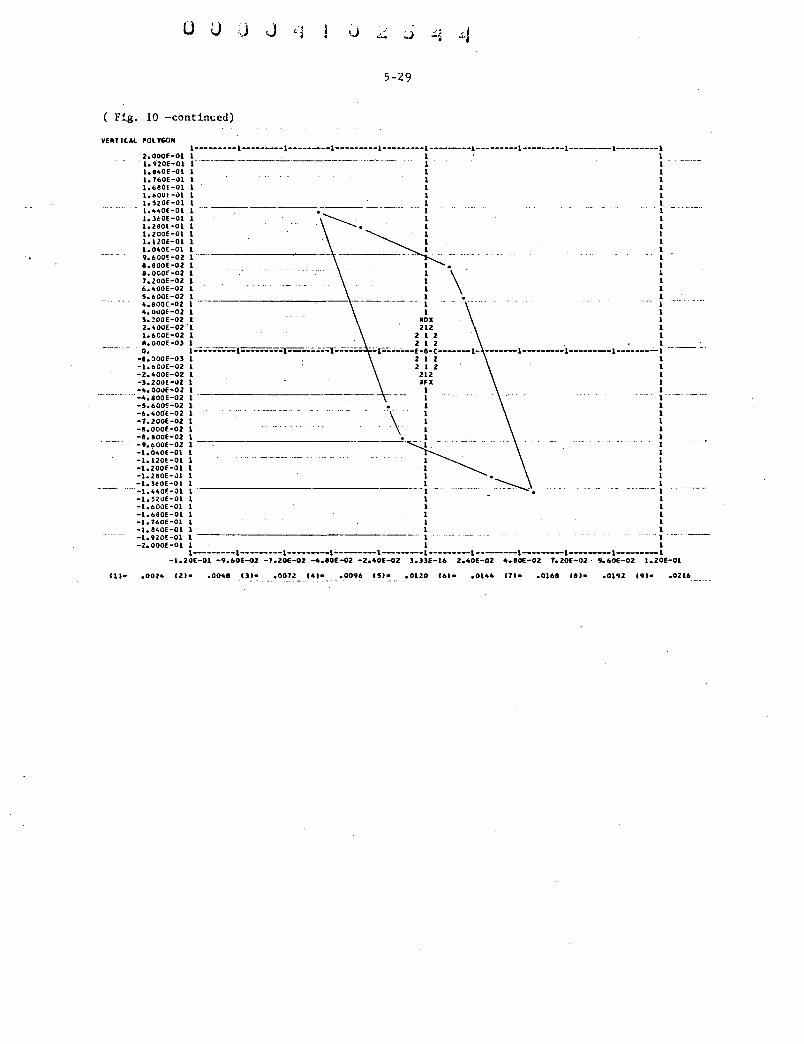
0 u J

5-29

( Fig. 10 -contin~ed)

VERT I tAL 'OL YGON

2.oooe-o1 1o~20E-01 t.e40f-Ol 1.760£-~1 1o680E-01 le&OOF-01 leSZOE-01 t.~ltOf-01 1oltOE-01 t.zeot-ot 1.zooe-o1 1.120£-01 1.040[-01 9.600'E-02 a.eooe-oz a.ooor-oz 7.200£-02 6.~00£-02 5.bOOE-02 4.800£-02 ~. 000~-02 l.~OOE-02 z. ~ooe-oz 1. 600E-02 A.oooE-ol o.

-e.oooE-Ol -1.60~£•02 -2.400£-02 -3.20~£-~2

1---------1-----'----1---------1---------1---------1-------1--------1--------1------1---------1 1 1 1 l ·-----·-------------·-····---·-· l 1 1 1 1 1 1 1 1 1 1 1 1 1 1 1 1 1 -----------~----- 1 - 1

1 :----- 1 1

l --~ l : - ~ .\ ~ 1 1 1

~ ~ . ~ 1 1 1 l XDX 1 1 212 1 1 2 1 2 1 1 212 . 1 1-'-:;---==--=1=~--.-:.;;:;;.;~;.;.;-..;:;;-- -r=---·--e-a-c----1- ---1-----1-----1--'-..:..-""-'-1 1 2 1 2 1 1 2 I 2 1 1 212 1 1 XFX 1

-"• OO~E-02 1 1 1 _________ _ -4.aooe-o2 -5.600£-02 -•.~ooe-o2 -7.200£-02 -a.oooe-02 -a.aooE-02 -~.600£-02 -1 • OltOE -01 -1.120£-01 -1.200£-01 -1.280E-J1 -l.ltOE-01

··-·· -1.HOE-~1 -1.520£-01 -l.600E-Ol -1.680£-01 -1. 760E-Ol -1.8<0£-01 -1.920£-01 -z.oooe-ot

1 1 1 1 • 1 1

: \ ~ ~ ~ - ----_-_-_-_-·-~------ ~-1 . - -~ ~. 1

~ --~ ~·. --- ~ 1 1 1 1 1 1 1 1 1 1 1 1 1 1 1 1 ... 1 .. 1 1 1 1 1--------1--------1--------1'--------1------1-------1------1-----1----1----1

-1.20£-01 -9.60E-G2 -7o20E-02 -4.80E-G2 -2o40E-G2 lollE-16 2o40E-02 4o80E-02 To20E-02 · 9o60E-02 1oZOE-01

Ill• .0024 CZI• .oon 141• .oo96 ,,,. .otzo t61• .ot44 ttl• .ot6a eel• .0216

5-30

OATE•6Il8171tt

ADD 2 NO PA~T OF SYSTEM MUON COLLECTOR (ffft 2.'916£•02·--··

,001 .471 .ooz

liUNIT1 51UNIT2 9(1J~ITJ

lliUNIT4 l71UN 175 2liUN IT6 251UNIT7

- 2~lYECl

15.0 15.0 15.0 15.0 15.0 15.0 15.0

22.000000 zz.oooootl 22.000000 22.000000 22. oocooo 22.001000 22.UOOOOO

311 PLOT! H. 000000 381PLOT2 24.000000 451 Pll HS 24.000000 521Silll 24.000000 5918EAHl 1. 000000

. 6710Al 16.000000 701 STOY1 21.000000 7<tOAZ 16.000000 77(POL Yf. -13.000000 791101 u.oooooo 8lC L 1 3. 000000

. 83101 5.000000 871L2 3.000000 89102 5.000000 931L3 3. 000000 95lo.u l6.oooooo 9~IDH I 16.000000

10liOA5 1-·- 16.000000 1041FFI I 2.000000 10718Ml I 4,COJ000 11118M2 I 4,000000 115 I FFZ I 2. 000000 ll81l4 1 3.oooooo 120103 .. 1 5.000000 1241L5 I 3.000000 126104 I 5.000000 130IL6 I 3.000000 1321 sun 1 6. oooooo 1361CON1 I -10.000000 14liColN 1 -1o.oooooo l46CCON J -to.oooaoo l5lCCON2 I -10.000000 1561102 I 13.000000 15811~3 I 13.000000 l601SPECPII l3.00u000 1t21L7 1 ... 3.000000 164105 I 5.000000 1681L8 I 1.ooaooo 170106 I 5.000000 1141l9 I 3.000000 11H07 I 5.000000 l80illO 1 3.ooomoo 192(0A6 I 16.000000 L8510a7 1 u,ooaooo IA8U~3 I 4oU00000 1~2lB•4 I 4.00JOOO 196llll I 3.000000

6.0 1.0 2.0 5.0 s.o 9,0

.. RAO

" " T ll.O GEV

o.o 10o.o

1000,0 1oo.o

1.0 10.0

t.O .. 6.000000 . o.oooooo o. 000000

.020000 o. 000000 -.020000 o.oooooo o.oooooo t.oooooo 4.000000 5.000000 .ozoooo

.. 29.000000 -8.000000 16.000000 s.oooooo z.oooooo 1.000000

o.oooooo o.oooooo o. 000000 o. 000000 o. 000000 • 005000

.o3oooo o.oooooo o.oooooo -.oosooo

.. -.030000 o.oooooo o. 000000 o. 000000 -.030000 .030000

.120000 .140000

.z~oooo .asoooo • 030000 • 005000

---1.000000 -·-- . . -6.000000 6.000000

• 098000

o.oooooo o.oooooo o.cooooo

.030000 o.oooooo -.030000

o.oooooo -.030000

.002000

.050000

.030000

.sooooo ·--;.;z.o88l08 ·· --1-.oooooo ·-··-··-· · ··

.zooooo .282000 .400000

21.000000 4.000000

·-. 5. 000000 zo.oooooo

.291000 .291000

20.000000 .400000

2.885813

o.oooooo .098000

- .076000 -o.oooooo

• 527000 .527000

-o. oooooo

.282ooo -~s.oooooo

.060000 .za2oou .200000

5.000000

4.oouooo .1ooooo -1.000000 z.oooooo

-· -1.oooooo --·z.oooooo -3.000000 4. 000000 -3.000000 4.000000

t.oooooo 4.000000 2.000000 .2ooooo·--.2~2000 -5.oooooo .ObOOOO .zazooo .060000

5.000000

.2e2ooo -5.oooooo .750000-

4.000000 s,oooooo

. ,]90000 .390000 .750000

.uoooo olOOOOO

-,uoooo -.610000

1.000000

o.oooooo o.oooooo

1.oooooo

.1ooooo o.oooooo

- -- o.oooooo o.oooooo o.oooooo

t.oooooo

1.oooooo

1.oooooo

o.oooooo o.oooooo

.oOlOOO

.001000

.001000

.001000

o.oooooo o.oooooo o.oooooo o.oooooo o.oooooo o.oooooo

1.oooooo .030000

o,oooooo .160000

o.oooooo

19f'CQ8 • ,.010000 .282000 -.:.J.20)8)5----l.000000 - ~-----~- -·- -·· ·-· ----··-

2021ll2 I 3,000000 2041LXO I .3, 000000 2061~9 I 5.010000 2101 ll3 I 3. 000000 Zl21SLIT2 I 6,000000 Z101CON3 I 10.000000 . 221CCON4 1 1o.oooooo ZU II 0~ I 13. 000000 2281105 I 13. oooooo 2301SPEC"UI 13,000000 2'21LH I 3.000000

.060000 .zazooo .282010 .400000

5.999515 1.oooooo

4,000000 .100000 .100000 ·~1.oooooo ---z,oooooo-·· o.oooooo -3.000000 4,000000 o.oooooo

t.oooooo '4.000000 T.oooooo

.8ooooo

,001000 ,oouoo

o.oooooo 1.000000 1.000000 1.oooooo 1.000000 1.oooooo 6,000000

-o.oooooo o,oooooo o.oooooo o.oooooo

CAS! NUI<OIO.

-o.oooooo -o.oooooo -o.oooooo -o.oooooo -o.oooooo -o.oooooo

.uoooo

Fig. 5-11. Transport output for the complete ~-~ channel of example 2.

1- o-c

u u d u , ..

5-31

(Fig. 11 -continued)

PLOTS PLOTS PLOTS PLOTS &UN

Zo998E-01 l.OOOE•OO 2.998£-0l loOOOE•OO 2.998E-Ol •• XCM

VECTOR lUI o. VECTOR ZIBI Oo

loOOOE-02 1.000E•OO lee .XPCRAOiee •• YCM

o. o. o. o.

z.998E-01 l.oooE•oo loo .YPIRAOioo ooSI14

o. o. o. o.

--------- ·--···--···-·- ·---·---- VECTOR 31CI 2oOOOE-OZ o. 5 • OOOE -OJ o. o.

5ol08E-O~ loOOOE•OO loo oOPIPC loo •••• CON

o. ·0.0000 lo oooE •Oo. ·o.oooo l.oooE•Oo -o.oooo l.OOOE+OO ... 0.0000 loOOOhOO -o.oooo t.OOOE+OO -0.0000

z~.o z~.o

z~.o 2~.o 1.000000

I 29.01

VECTOR 4 IDI Oo leOOOE-02 O. J. OOOE-02 Oe VECTOR 51EI -2.oooe-o2 o. -5.000E-OJ o. o. VECTOR 6IFI O. -J.OOOE-02 0. -J.OOOE-02 o.

0 o. 0000 " o. 0000 .. o.oooo .. 1.0000 6.0000 l -.0300 ~ .0300 RAD -.0300 M .o3oo -o.oooo 4 ··.1200 ·cev--.1~00 GEV . ·- ·- o0020 GEY o. 0000 o. 0000 5 o 2500 N • 1500 RAD o0500 M ol600 0.0000

ol3000 GEV ------------------------------------------------------ IU141 - 59

VECTOR VECTOR

.... - ---·-··· VECTOR VECTOR VECTOR VECTOR

lUI 21BI 31CI 41DI SIEI 61FI

0.000 oOZO M LENGTH- 0.000 M OeOOO • 030 R AD Oe 000 o.ooo .oo5 " o.ooo o.ooo 0.000 .030 RAD OeOOO 0.000 OeOOO o.ooo o.ooo " o.ooo o.ooo o.ooo o.ooo OeOOO 0.000 PC 0.000 0.000 0.000 0.000 0.000

•• xcM lee eKPUtAOt •• eaYCM lea eYPCRAOI ..... SCM 1 •• aOPCPC' I•• o. o. 2.oooe-oz o.

-z.oooE-oz o.

o. o. o. o. o. o. o; o. o. 5oOOOE-Ol o. o. 3.oooe-oz o. 3.oooE-o2· o. o. -5.000E-03 o. o.

-1.oooe-o2 o. -3.oooE-02 o.

o. loOOOE•OO 1oOOOE•OO l.OOOE+OO loOOOE+OO l.OOOHOO

•••• COM ..o.oooo -o.oooo -o.oooo -o.oooo ·0.0000 -o.oooo

PAR 16.0 Ell 21.0 PAR 16.0 OR 1FT !ieO OUAO 5.00 DRIFT loO OUAO 5.00 DPIFT 3.0 PAR 16.0 PAR 16.0

-8.0 -6.oooo -1.00000

6.0000 ST~Y.l - TO

PAR; 16.0 RORAT ZoO BEND ~.000

.I 16.01 loOOO N

• 500 " .zoo " .zez M • .r.JO M ZloOI

4t.OI I 5.01 20.000 0

.291 "

o C9800 ------· ---- . --·-···--

-2.0881

2.8B58 T

loOO N

1.00 "

-.J~ "

·" .. o. ooooo--------

• Cl9800 .07600

-o.oo T o52l T .oo ZOo 263 Dl

I oiZl M I BEND 4oDOO. ~291 H.·····- o52l r· · ·~·oo -.--zo. zu o 1 ·· ·· ·· --- ·····- --·- ··

ROPAT z.o 20.000 DRIFT loO .400 OUAO 5.00 .2Bz DRIFT J.o .060 OUAD s.oo .zez DRIFT loO .zoo SLIT 6.0 4

0 .. " "

-o.oo T

-5.0000 loOO M

H 5o0000 T loOO M M .1000 .. .1000 ..

I ol23 N I

-.21 "

o.ooo o.ooo o.ooo o.ooo o.ooo o.ooo

•• XCM t •• eXPCRAOJ •• lUI o. o. 21BI lo0l6E-02 -lo503E-02 31CI . -2.523E-Ol -l.H6E-02 4101 1oOHE-02 -6.0l9E-OZ 51EI Z.405E-OZ -l.560E-02

A-TABLE NO.;• 2 LENGTH• 1.000 " A-TABlE NO.• J UNGT ... le500 M A-TABLE NOe• 4 LENGTH• lolOO M A-TABLE NOe• ' LENGTH• lo98Z M A-TABLE NOo• 6 lENGTH• 2o38Z II

A-TABLE NO.• 1 LENGTH• 2.312 M A-TABLE HOe• 1 LENGTH• Zo613 M

A-TABLE NO.• 8 LENGTH• Zo964. M

LfNCTit• 2•9•4 M lfiiGTH• Jo364 " LENGTH• 3.6~6 " t..fHGTH• ,. l06 " UNGTt<• , .... " lf~GTH• 4ol88 M LENGTH- 4olBI M

A-TABLE NO.• 9 A-TA8LE NO.• 9 A-TABLE ND.•lO A-TAIL£ NO.•ll A-TAILE IIOo•U A-ueu NOo•U A-TABLE tl0e•l4 eOl) fll lEIIGTH- 4.188 .o4S .-,,o -.011 .oo1 " o.ooo o.ooo .0)6 R.AO o.ooo 0.000 • TU .052 .. .370 .~24 o.ooo o.ooo

o.ooo o.ooo o.ooo o.ooo o.ooo

Ll -81 Q1

_., lJ -n liZ - " LJ - 9;

Ffl -104

'"' -107

IMZ -111

FF2 -115 l~ -Ill Ql -120 l5 -124 Q~ -U6 L6 -uo SLITI -132

"

OoOOO PC ... ,.. . .. o.

.YPCRAOI •••• SC" 1 ••• OPCPC lee •••• CCIIII

o. 6.l86E-03 4ol51E-06

-6.186£-03

o. o. o. -o.oooo o. -4. TJJE-04 t.OOOE+OO -0.0000 2.81oE-o2 -1.983E-D2 a.oooE•Oo -o.oooo 2.2ue-o2 -~.90TE-OZ a.ooouoo -o.oooo

-2.810E-D2 l.laeE-02 a.oooE•OO -o.oooo

VECTOR VECTOR VECTOR VECTOR VECTOR VECTOR 6(FI lo076E-02 loOl~-02 -4.UlE-06 -Zo2UE-02 4ollU-02 loOOOE+OO -0.0000

TRANSFORM 1

·-6o6~24E-Ol lol823E-04 · 2oBU4E-02 -l.5055h00

o.·--··· o. lol572E•oo S.ll96E•OO o.

o. o. o. o.

-9.6769£-0l -1.6199£+00 o. o.

DRIFT 3o0 .200 H ouAo s.oo .zez " DRIFT 3.0 o060 M OUAO SeOO .282 fill DRIFT 3.0 .060 M QUAD 5.oo .282 " Dfi1FT loO .750 M P.P &6.0 4eOI PAR. 16.0 5o01 8END 4.000 .390 M

8END 4.000 .390 ..

o.

-5.0000

5o0000 T

-5.0000 T

.uooo

.10000 -.630 T

-.630 T

loOO M

1.oo "

1.00 "

• oo

.oo

o. o. lo3838E-04 lo314ZE-Ol o. o.

Oo lo0l62E-OZ Oo -1. 5030E-OZ o. o. o. o. loOOOOE+OO -4. T329E-04 o. t.ooooe•oo

-.21 "

o36 M

-.21 "

I -32o464 Dl ( -.688 .. I -32o46~ Dl

·- I -.681 M DRIFT 3.0 .750 H OUAD 5.01 .282 H -3.2038 T 1.00 ... ~- -.44 " DRIFT 3.0 .060 M DRIFT. 3.0 .282 " OUAD 5.01 .2az " )5.99filS T loOO " oll " DRIFT 3.0 .~oo" ··-- ---- --·-

SLIT 6o0 4 olOOO H olOOO II FIT lOoO -1 OoOOOOOOI .001000

.412325 I'IT , ... _, • loOOOOOO/ .eo&oeo

-.ooonz .. ·-- ---···----·-·. . -------·-···

A-TABLE NOo•l5 LENGTH• 4e381 " Ll -·;.162 A-TABLE NOe•l6 LENGTH• ... 670 " 115 -164 A-TABLE NOo•ll LENGT ... 4.730 " ll -161 A-TABLE NO.•ll LENGTH- 5.012 " Q6 -110 A-TABLE NO.•l9 LENGTH• 5o072 M u -lH A-TABLE NOe•20 LENGT ... 5.3~4 " Ill -116 A-TABLE NOo•21 LENGTH• 6ol0~ II LlO

.. -180

A-TABLE N0o•Z2 LENGT ... 6.49. " 8M3 -Ill

A-·TABLE NOo•Zl LENGTH• 6.884 " IM4 -192

A-TABLE N0.•2• LENGTH• 7.634 " Lll -1'16 A-TABlE NOo•25 LENGTH• lo916 " Ql -191 A-UBLE N0.•26 LENGTH• 7.976 " U2 -202 A-UBLE N0.•27 LENGTH• 1.251 " LXQ -z~ A-TABLE fol0.•28 LENGTH• lo540 " 119 -206 A-TABLE N0.•29 lENGTH• 1.940 " LU -uo A-TABLE NO.•JO LENGTH• •. ,.o " ntu -zu

5-32

(Fig. 11 -continued)

VECTOR VECTOR VECTOR VECTOR VECTOR

··- ··---·-·----·veCTOR

lUI 2181 31CI 4101 51EI

... 61FI

• .XCM I •• o. 1.oo~e-oz

1olT6E•OZ z.Z46E-OZ 8o4Z7E-03

•ZoZ76E-Ol

o.ooo o.ooo o.ooo o.ooo o.ooo o.ooo

• XPI RADio • o. 9.798£-02 3o822E-02 la440E-02 1.5T8E-OI lo816E•OI

.OIZ II

.103 uo

.011 ~

.040 RAO

.219 " o.ooo PC ...... 1 •• o. o. lol42E-02

-9.~69f-Dt •lo142E-02 ~.969E•06

lEIIGT,._ a •• 4G M -.an o.ooo o.ooo o.ooo o.ooo .943 -.~75 .~65 o.ooo o.ooo o.ooo o.ooo o.ooo o.ooo o.ooo

.YPIRAOt •••• SCM I ••• OPCPC 1 •• o. o.. o. o. -6.Z61E-Ol 1oOOOE•OO 3.7HE-02 -8.292£-0Z lo OOOE+OO 1ol10E-02 •2ol18E-01 loOOOE+OO

•lo TUE-02 7.040E•02 1.000£+00 •lo JlOE-02 lo993E-Ol lo OOOE+OO

•••• COli -o.oooo -o.oooo -o.oooo -o.oooo -o.oooo -o.oooo

TU~1FOR~

loll31E•OZ 4ollllE-Ol -Z.9114E+OO •Zo li&U+OO o. o.

o. o.--3.8328E+OO -6.8523E+OO o. o.

o. o. o. o. o. o. ZoZI48!+00 •Jo1UU•04 Do

7.46,8IE+OO 4.J660E•Ol o. o. o. leOOOOE+OO o. o. o •

a.o-e-oz 9o7 .. 4E•DZ o.

o; -6oZ.05£•0)

l.OOOOE+OO DRIFT 3.0 • aoo " A-UBLE NOo•31 LEHGT,._ .,.140 " LH -212 LENGTH 9. 740'1

J TYPE .• III l •Pu ··· JiPv· · H-8EAM V·SEA~ H·CENT V•CENT HRAYL VRAYl 1 1.059 o. 0000 z.ooooe-oz 5oOOOOE-Ol o. o. o. o. 1 1. 059·8EA~1 z 3.081 1.oooo 3e6056E-02 3.0414E·02 o. o. o. o. 2 3.081-i.l ) 5.08) 1.5000 9o8000E•02 9o8000E·02 lo583~E-02 2.5950E-OZ o. o. o • o. 3 5.083-Ql

• 3.0~7 1. 7000 • 1057 lo68T2E•02 o. o. o • o. 4 3.0BT·l2 5 5.08~ 1.9820 9. eoooe-02 9.eoooE-02 .IIH 8oi44UE•Ol o. o. o. o. 5 5. 089-02 6 3.093 2.3820 a. 9580E-02 To4343E·Ol o. o. o. o. 6 3.091-ll 7 4.107 2.6730 9.8000E·02 7e6000E-02 7.5519E-02 1.2BllE-02 o. o. o. o. 7 4.107-8"1 8 4.111 2. 9640 9. SOOOE-02 To6000E-02 5.2189£•02 lo9l53E•02 o. o. o. o. 8 4elll-8M2 9 lollS '· 3640 2.4674E-02 2.6479E-02 o. o. o. o. ~ 3oll8•l4

10 5ol20 3.6460 9. SOOOE-02 ~. SOOOE-02 1. T08SE-02 lo~65TE-02 o. o. o. o. 10 5.120-Ql 11 3.124 3. 7060 1. 7892E-02 lo 590IE-02 o. o. o. o. 11 3o1H•l5 ·u 5.126 3.9880 9. SOOOE-02 9. eoooe-o2 1o6162E-02 ~.5425E-Ol o. o. o. o. u 5.126·04 13 3.130 #te\880 1o l285E-02 6o 7858E•03 o. o. o. o. 13 3ol30-L6 14 6.132 4.l880 1. OOOOE-01 1oOOOOE-01 1ol285E•02 6o 7858E-03 a. o. o. o. 14 6o1l2-SL t.Tl 15 3.1t.2 "'· )tt80 l.S968F-OZ •• ~285£-02 o. o. o. o. 15 3o162-i.7 16 S.lb(t •• 6700 9.8000E-02 9e BOOOE-02 3.4340E-02 lo6168E-02 o. o. o. o • II> 5.164·05 17 3ol68 •.noo 4el032E-02 1. 52HE-02 o. o. o. o. 17 lol68-i.8 18 5.170 5.0120 9. 9oooe-o2· 9.8000E~Ot 5.0645£-02 lo8024E-02 o. o. o. o. 18 5.170·06 19 lol 74 5.0720 4. 7714E-02 2.0222E·02 o. o. o. o. 19 3oiH·L9 20 5.176 5. 3540 9.8000E-02 9.8000E-02 5.551 TE-02 2.0560E-02 o. o. o. o. 20 5.1 76·07 21 1.1~0 6.1 ?40 .1369 7.6368E-03 o. o. o. o. 21 lelBO-LlO 22 4.188 6.1t940 .1600 I.OOOOE-01 o155T 2.054TE-02 u. o. o. o. 22 4.188·9•1 23 •• 192 6. 8Rlt0 • 1600 1.0000E-OI .1258 3.4128E·02 o. o. o • o • 23 4.1~2-8"4

~·z• 3.lq6 ·7.6340 -··. --·-· .. 2o5493E-02 6o0471E-02 o. o. o. o. 24 3.196-Lll 25 5.198 7.9160 9e SOOOE-02 q.eoooe-oz 1.05TOE•02 5o254lE•02 o. o. o. o. 25 5.198·08 26 3.202 7.97t0 1. 71~5E-02 4. 7226E·02 o. o. o. o. 26 3o202·L 12 27 3.204 8.2580 5o0021E-02 2.225ZE-02 o. o. o. o. 27 3o204·LXO 28 5.206 8.5.t.OO 9.8000E-02 9. SOOOE-02 5.2459F.-02 ~. 3133E-03 o. o. o. o. 28 5. 2.0~-Q9 29 3.210 8.~400 1.2482E•02 1.1424E-02 o. o. o. o. 29 3.210-ll)

-30 6o2l2 a. q,..oo 1. OOOOE"Ol -1~ OOOOE~Ol lo 2482£-02 1oi424E•02 o. o. o. o. 30 l>o212·SLIT2 31 3.232 9. 7400 7o1411E-02 4.259~E-02 o. o. o. o. 31 3.23Z-ll4

J TYPEel J I l HRAY2 YltAY2 HRAY) V~AY3 HRA.Y4> VRAY4 HRAY5 VRAY5 HllAY6 ~RAY6

1 1.059 o.oooo o. o. 2o OOOOE-02 5.0000E•03 o. o. -2. ooooe-oz-5.ooooe-ol o. o. 2 3.081 1.oooo o. o. 2.0000E-02 5.0000E•Ol 3. OOOOE ·02 3 • OOOOE •02 -2. OOOOE -02 ·5 oOOOOE-03-3 • OOOOE ·02· 3 • OOOOE- 02 3 5.0R3 1.5000 o. ·o_----- 3.32~6E-02 2.2805E•03 6o8140E·02 2 • 564~E-02-3. l296E-02-2. 280 5E·Ol·6o BHOE-02·2. 5849E•02 4 3.0~7 1.7000 o. o. 4o4978E-02 3.2758E-04 9.5652E-02 lot868E-02-4. 4978E•02•3o 2758E•04-9o 5652E·02-1.6968E•02 5 5.089 lo982U o. o. ~t. B65oe-oz-z. 5a.r.ee-o3 .1069 7.7229E-03-4.86SOE•02 2e58413E-Ol -.1069 -1.1 ZZ'9E-03 6 3.093 2.n2o o. o. 3. 523H•02-7o 3022E•03 s. 2359E ·02-I.3949E-OJ·l. 52lbE·02 1 • 3022E·03·8 • 235~E-02 1.3q4q£-03 7 4oiOT 2.6130 5.0923E-04 o. 2. 8451E-02-1.0104F.·02' 7 .0669E-02- 1 .~OT8E-Ol-2. 74l2E-02 1.0104E_;02-6.9651E•02 7e9078E-03 a 4o11l 2. 9640 lo 973~E-Ol o. 1. 9162E-02-Io 2906E-02 5.1251E·02-Io442IE·02-1o 5214£-02 lo 2906E·02•4o7304E•02 1o4421E·02 ~ lollS 3.3640 4.9223£·03 o;·---. a. 5639E•03-l. 522 TE-02 2.9326E-02·2.166lE-02 1.2808£•03 1. 522TE-02·1.9481 E-02 2.16o3E-02

10 5.120 3.6460 9. lbBlE-03 o. 4oi328E•Ol-I.OI61F.-02 2. 5901E-02-I.6828E•02 1. 5403E-02 1. o 161£-0Z-6. 3644f-Ol l.t828E·02 ·u 3.124 3. 7060 1oi543E-02 o. 3. 69~~E-Ol-7. R239E•03 2. 7 622E •02·1· 38HE•02 1.93~ 1 E·02 7.e239E•Ol•4 .5 358E-03 lo3843E-OZ 12 5.126 3.9.80 1. 3168E-OZ o. 3.64iOlE-04 l.046ZE-03 2. 2806E-OZ-4.<ft20<4tf-03 2. 7166E -02-1. 041>62E -03 ~. 7 Z941>E-Ol 41> .~ZO~E-Ol 13 3o130 4.1880 1.0762[·02 o. -2.52lOE-03 6o T858E-03 t.OT67E·OZ 4.151lE·06 2.404TE·02-6oT858E-Ol 1.0T5tE-02·4.1513E-06 14 6.132 4.1880 lo0162E-02 o. -2.5230E-Ol 6o785$E•Ol 1.0T6TE-02 ~.151lE-06 2.40~1E·02•6oT858E•03 1.0756E-02·4.1513E-06 15 3oi6Z 4.3880 7. 7559E-Ol o. ·---~5.4151£-03 lo2525E•02•Io 211 TE-Ol 4.428TE•03 Z.092TE·OZ·Io 252SE-02 1o&783E-02·4 .U87E-03 16 !i.l61t 4o6TOU 6.6755E-03 o. -1.2824£-02 lo4120E•02·2.1591E•02 7.8767E-03 2.6175E•02-1.1tl20E•02 l.4942E-OZ-7.87~7E-Ol 17 3.168 t\.7100 7.0829[-0) o. -1. 53~H-02 lo 3024[-02-Z. 727TE·02 7o9027E-03 Z.9512E·02-Io 3024£·02 4.1443E·02-T .q027E•03 18 5ol70 5.0120 5. HIU-03 Do -1.895bE•02 1• 3490E·02·3. 8520E-02 1o1953E·02 3. 0379E·02-lo 3490E-02 4.9~HE-02•loi953E-OZ ~~ !.174 5.0720 •• 7660£•03 o. -1. 7850E-02 1o4800E•02•lo 7248£•02 1. 3780E-OZ 2. 1382E -02·1.4800E-OZ 4 o6 780E-02-1oH80E-OZ 20 5.176 s. )540 lo ~6 T5E•Ol o. •2. 065!E-02 1. 3 7T3E•02-~. ft7l2E-02 1.5265£-02 2. 4588E•02-1.3773E-02 5o266 TE-02-1. 52HE-02

- 21 3.1~0 6.1040 •2. 2175£-03 o.··----5.0498E•02-7.6313E•Ol ·.1303 •2o900TE-04 4o606JE-02 7o6313E-Ol .1259 2o9007E-04 22 1t.lH8 6.4940 -5.0082E-03 o. -S.8l85E-02-1.6761E-02 -.1~12 -e. 378'JE-03 ... 8)6qf-02 lo8161E•02 o1412 8.3J&qE-03

Z3 •·t•z 6o8840 -e. 3B49e-os o. •5o017~E-02-2o98~2f-02 -.1210 -l.6468E•OZ !ol405E•02 2.9892E•OZ .1102 1.6468E -oz 24 3.196 7.6340 -1.~763£-02 o. -1. 9715E-02·5 oi296E·02-3.975~E-02-3o2023E·02·9. 7512E-03 5oi296E-02 1o02l2E-02 3o2023E-02 25 5.1~8 f.Ql60 -2.195TE-02 o. -1. 32~1E •02-~.~233E-02-Io 5~0~E-02·2. 8360~·02-3. 0622£-02 4. 4233E·02-Zo 8009E-02 z. 83t0(•02 Zt 3.202 7.~760 -2.4~5tE·02 o. -1. 2831E -02-3.966 3E -02-1. Z242E -02-2. s 6 l4E-02-3. 6481£-02 3.9663£-02-3.7070£-02 2 .5634E-02 27 3o204 8o2580 -3. 7343E•02 o. -1. 0665E-02·1• 818 TE -oz "• 9705E-Ol·1• 2 821E-OZ-6o 40ZOE-OZ 1. 8187E•OZ-7.'1656E-02 1oZ821E-02 Z8 s.zot 8.5400 •2o9100E-02 o. • Jo 5268£•03-3. 5078E•OJ 1o670JE-02-5 o24~lE •OJ-5 • 46 74E•02 3o 5078E-03-7 .4904E•OZ 5.2491E-OJ 29 3.210 1.9400 1.0094£•02 o. 1.1760E•OZ 1ol424E~Z z.Z44JE•OZ•9oM9U•M .. 4169E...,-lo14ZU-eZ-ZoZ1.U-OJ , ... •ze-• JO •• 212 .... oo l.OOME-Ol o • l.l760f·OZ 1o14Z4E-GZ Zo!4Uf-i!Z-11.•••ZE- lo416U-eJ-lol4ZU-oZ-ZoZ76ZI-OJ ..... 1£-M Jl •• uz •• ,.oo •·•uu-oa o. ... au~-oz ... une-oz J.J .. H-oz •• -. .. 1-oa ...... .... unt-ea .&4)0 -•·-•-oz

u J J

5-33

IIIIITAL 't'lCTO .. f'L01fl0 ON 8U.Ml.ll'lt I Ul 0.0000 o.oooo DoOOOO o.oooo 0.0000 2 Ill o.oooo o.oooo o.oooo o.oooo o.oooo 1 "'. --~1120o -·o.ouo .ooso o.oooo o.oooo " 101 0.0000 0 0)00 OoDOOO oOJOO 0.0000 '5 U I -.0200 DoOOOO -.00,0 0.0000 o.oooo 6 IFJ 0.0000 • 4 0100 OoOOOO •oOJOO 0.0000

't'flltiCAl IU" ..O.UOfn'Al tU•

o.oooo 1.0000 1.0000 1.0000 1.0000 ......

-o.oooo -o.oooo -o.oooo -o.oooo -o.oooo -o.oooo

.liDO .09l1 .oJJJ .05'50 .0)61 .Oil) OeO .029) oMIT ootiD ollfJ ol .. f 0 lT6 ·---------·---..:-:...;._.;. • ..;.·..:.:.·.;.:.._:. • .:...;.. ___ _.,;:.·~----·..;..::.;. _____ • ______ ·~------·-------·--------·---------·-..:--:..-..;..::..-.=.-o.ooo u n • n o .o9J Ll e J5644 n o ••• , l1 • "' l46 , 0 • nz u • "n z -.. su o 0 )90 l1 I ' ' 15 l 4o4o Ul 0 .41lll .... ,, • .,,. .,-.,.. ll 146 " l •• , • 0 ... z U 144 U Z 46 I D eU9 ll _.. J5 l U6 II 0 .en u •• n z ,,., e o _.,,. l1 M6 " z , 46 • 0

1.011 Ql 0000 46 " Z U .W.II OOOOOOOOOOOOQQOOQODOOOOOQOOO lol6901 0 46 )SJ U 461 0 loZ66 01 0 46 JU U 441 0 1.16<11 Ol 0 46 JSZ U u I 0 1.4U 01 0000 46 UZ U 461 OOOOQOOOOGOOOOOOGOOOOOQOOOOQ 1.n1 u: '" u u 44 • o l.6U lZ <W IJ U 46 t G" t.nJ 02 0000 46 n U 460IOOOOOOOQQQCIOOOCIOCIOOOOQOO t.n.t 02 0 1M 5J U 046 I I.'MI 02 0000 U6 5U U 004600BOQOQQQQQQCIOOQOOQOQQQO 2.045 l) ti46SJ2 U 46 I D 2.UJlJ 1HZ U 461 0 2.140 l1 IU461 U 461 II z.nt u an ._. u 441 o t.4JS 11111 111111111111111111111111111111,..111111111 SJ M.Z JS 461 -~~~-IIHifii-IIQIIIII-MIIIIIIIIIIII"""" ........ 2.nz B"'l .. 15164 z u 6 a "' .Z.6J0 flllll tlllllllitMI'IIIIIII-1111111111 .... 111 15JM 2 5 461 IIIIIIIIIMIUttiiiiiJII_tii_III.IIIIII.._.,...IIIIIIM

1.121 I"'Z ~~~~~~--"'""'"'""'""'"' I 564 Z 5 461 IIIIIIIIIIIIIUUIIIII..,.,._--111111,._....... t.tzs P.Z . .•. I 64 1 5 61 111 • z.•2Z 11'12 IIIIIIIIIIIIIIIIIIIIIIIIIIM .. tttMM I 65) 2 5 MIIIIII-1111111111111'11111111111--1111111111""*"'*-

J.Ol• l4 I 611 2 !I 64 0 J.lU l4 I 64SJ U U 64 0 J • .Z14 l4 I 64 U US J 64 0 J.JU l4 I 64 SJ l5 J 684 0 J.40. l4 I 64 n ZSJ 61 o4o II s.S06 OJ 0000 I 64 5J l 5 6 II 4 OOOOOOOOOOOOOOOCIOOOOOOOQOQOQ ).604 OJ QQOQ I 64 5J U 6f I 4 OOOOOOQOOOOOOOOOOOOOOOOOOQOO J.JOl l5 164 5J ZJ62 J o4o D J. n• 04 OOQQ ,._. 5J M ll 54 OOOOOOOOOOOOOOOOOOOCIOOOOQQOQ , .... o. o MSJ6 za s o J."J 0. 0000 6o4oJ56 ll 4 S OOQOOOOOOQOOOOOOOOOOOOQQGHCI 4.0"1 l6 U64ZJ6 14 5 0 4 .... l6 " o4o6) .. ' 0 4.181 Sllfl I SSSSUSSUSSSSSSSSSSSSSUSS 4.216 l J ' ' 44l4J26 ' 0 4.JU l J IJS 46 Z4J 6 S 0 o4o.410 OS 0000 J5 46 l Z4 6 OQQCIOQOOQOQQQCICIQQOOOOOQOOOOQ 4.~UI OS 0 US <Wo l Z J 4 M 0 o4o.6TS OS 0000 IU 46 .Z .Z J 5 N OOOQOQQQOQOOOOOOOOOOOOOOOOOO •• nJ ll an46 2 .z J '" 6 o 4.170 06 0000 I J~ l Z J 5 4 6 OOOOOQOOQOOOOOOOOOOOOOOOOOOCI 4.'96 J 06 0000 I JU Z Z J 5 4 6 QQOOOOQOQQQOQOOQOOOOOOOOQQOQ s.o6<J l• • '" 22 J s 4 • o 5.162 Ol' OOQQ I 46 U J 5 o4o 61 OOOOOOOOOOOOOOOOQOQQOOQQQQQO 5.260 Ql' 0 • .., .z , ... 0 S.JU QJ QOOO I 465 l S 68 OOOQOOOOOOOOOQQQOOOOOOOQQQQQ "·"" llO I "6JS 2 5 .. 0 s.nz uo e 46JS z s 6 • o 5.6-4'9 llO I 46IS l U 6-41 D s.J4l' liO I 4615.2.1: U D 5.144 l \0 8 465JZ 5J M I D ,.'941 llO I '622 5 J 6 4o8 D 6,.0]. llO UJ 46Z 5 J 6 41 D 6. U6 llO SJ 642 5 J 6 41 0 6.U4 lot] !till SJ M2 .Z S J 6 41 _.... .. 6.Jn 6111) Ill ., ... z l ' J • 41 Ill 6.421 IMJ Ill 151 64 l 5 J 6 4 " •• ,,. ,,., 1111111 ., 64 l ' , • 4...-.... 6.6ZJ I'"' 111111 15J 64 l 4 _ _.,. •• nt .,.. 111 , ,, .,. " 6.111 I"" It I SJ 64- Ill ••• u ••• "'" • ,, 64 --~~~~-l.OU lll I tJ 64 D l'.uo llt 1 ,, .. o 1.201 Ul I U 64 D J.JOS lll SJ D 1.402 lll , 0 l' .. SOO lll 0 l.,.7lU 0 ?.ns Ql QOQQ QQQQOQOQQQQQQOQOQOOQOCIQQQOOQ

::::: :: ooo:: Q.QQIOQCQQIOQQO<OIO.OQOCOIOOOOOO"'OOOOO<IOOO,OOOQOQOOQ T.tiT LU . D •• o .. liQ 0 •• uz liQ 0 1.21'9 L:IO 0 t.l76 0. QOQQ QOQOQOOOQOOQQQQQOCIOOOOOOQOOO

-::;:~ :: 000: o.:otoOO<QQIQQO<QOIOOOCCICIOOCICIOOQ"'OOOOQ~QQIQQQCQQIOQQOCOIOGQ .. O I.M'9lU 0 ··1" llJ 0 I.MJUJ D 1.961 UJ D ..... lliU unsssssusssssussssusss t·.1JJ.-u4··- -----·------- ··--· . ··--,-9.156 u• o •.zn u• o •.no u• o ..... ll4 0 9.545 U4 ,. 0

-r.TU"l.lT"- ' • ----,-•• 1'40 u• s •

.uoo ·"ll' .oJJJ .osso .os.J .otu YOTIC&l au•

fC)Itll HI• .OOH Ul• .0059 Ill• .0011 141• .Dill (51• -·--~-"""TTJT---.oora czr• .wu cu• .• oc,, .. ,. ;oG"TT""TYl• .., ...

.OHJ .osn .un .1441' .n• M).llOinM. MM

.014l' 161• .oa?• Cl'l• .oro' nl• .OZJ9 191• .O.Z64 .O'O'fl rn-. .cnao en• .oue Ill• .Olo4oT ltl• .11(5!".--

Fig. 5-12. The beam line graph of the complete n-~ channel. Vectors 2,3,4,5, and 6 represent a 1% momentum deviated beam. Note the point of maximum momentum resolution after quadrupole QS.

5-34

x'( Rod)

--------------------~~~~~~~----~----~----~--~~ x(m) 0.10 0.15 0.20 0.25

XBL752-2259

Fig. 5-13. The horizontal phase space acceptance of the ~-~ channel of example 2 plotted as a function of momentum.

10.0

9_0

Acceptance of 8.0 pi channel alone

7.0

a: 6.0 VI ~

5.0

4.0

3.0

2.0

1.0

Acceptance of total system pian channel plus muon

collector

OL-~~~L-~~~~~~~~~~~ 0.09 0.1 0.11

P (GeV/cJ-

XBL75Z-ZZ.I

Fig. 5-14. The momentum acceptance as determined by the channel acceptance and production target for example 2.

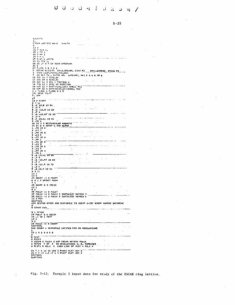
611 ft/~Co ..

u u

~~CAQ lATTf~£ ~U-l ~-4-~k

0 I J l 1S r "la( t. 1-; ,. .. 1 tS ,.D 1 tt; .... t 1~ f(r. 1 UNJ1'8 tt; 11 r:c:v t. 16 ·~ • " 1 7 Ct'. f)UftO IO~R.TtJOC: z• o zt ~.~1~ ~ a n u 1

5-35

C fS"•~ 51ZJI7• 6hJ,J55289 0 Ek•Z.~L--~'~1·6!9863 __ £)'_•_1~ PI l £'ITA l0An,cttr~G1 ,atGJOH•I « l'i ICL"' YJ, Ka~AT NO, l•~A,_.C:, Mal 1. 3 '- !J f)IP 6 t'i i!tr. tt 1: c;ru,u 1~ ZJ4 Z~ SliZ,ZI 16 31F. t1 V~C 1 "OYTtON J(

16 ~~6 12 t: -c-r.t YP POSTTION l!) '-1~ 11 St'HiT(~IC1 1 1JJe S'1Al.i..-R~ff·---------··-·-···---·-16 4JC: 22 SCFT (Sl (1,ZJ J•S,.All lfZ2 t 1 •,31" t c:,a9r, a o s 12. ODtS T·lL ,.~ 7. oc;-. i7 11: l ~t&oT··

3 1 Ll • ,, u.s 1e at 3 •• " s .t -tz,, ta .oz· l ,7 A s .6 -u.s?·u ai J • 2 "' 5 ,f 19,.1 11 C\ J ; ~~ L 16 2l l l RECHNClii.U NACNn~·

-!~.~~ ~~ 1/NPUT _I,_A!_I~~_!.!_H_A..,..------

J ·"" ~ .. ,os u J ... J ! - ,Ill!! •• 0 , , 116 L ·\ ,qs u o----· J ,4J s ' • as •• 3 •• J ~

,. • ~~ •• e

···-·-···-\------ ·-

-; ::~.~~- .. i·-.-r~··· ---~-J .z " •• 6 •15.~7 10 Ql 1 • 7 ' 5 ,6--ll,li 10 t'JZ

3 .z " .. , .6 12,, ·-.o···ni -------------·-----· ·--·-·-' J Ll 1l I ll • 2§ OUA.RT -t ! nUJPT 6 0 l 4: UPI}AT" REAM ~ . 25 QUART I 0 US£13 1 J 1 ~ 0 tS fULlf •1 25 fUll2 •1 ZS FULL• •1 ll 2 f .. ~

~~t~; f I"IT ALiZ!' MATQlk ~ FULl" ' JNITALii'£ . 11'TAIJ( .. ·-···-···-------·---- ..

SENTINEL AD~ SEC""D 0~0£11 •NO SEXTUPQL£ TO US£2~ l•IST O~O£R ~ATUX INTYP£•2 l .

. o suqT f"'!--·--·-----------· ··---·-·--------····-·· -··-···---·~ t •~•zo ZS fULLf 0 I USEZ~ 18 .t tO 1 !l;fJ"T 1J 1 q 0 2s ·FULL~ -.;-c-i-tsc-;• SENT I"f~l I!UN ESCU + SEXTU~OLE l ZZ100811Z z -a·sr.r ·-----·-

£XCITER FOR 9~ REVOLUTIONS

o rsc•' A US(ZS A orozn A Pl OT1

l fULL4 l US~ £SCU •UUik FULL' ~ 9' C 9q RrYOLUTIONS I, £, O[PEAT£5

' ~2.1 I tJCH LIN~ OF PLOT • qz.t "

·r. T.7 .1. 14 .. iO-lU l ~-·~E-PLGT VEr. Z l' 7 ~ •2 t.z •7 4 t PHA!r .. LOT VEC .J sr~TINfL Sc.frriT t"ffl

I

Fig. 5-15. Example 3 input data for study of the ESCAR ring lattice.

5-36

(SCA~ LH'TICE "'O•Z &.-io·7~

1( 'T')t J t.~. 1'HI"Ill1t'! JfL'NJTt I tr.~

.,.,w~JT? 1-:;.o 11fUNTT1 tr.n 15H1NtT.. 1S.Il tCJ ( I!"ITT~ 1~. 0

?Jfl!'~TTt; ~~.0 Z.,.t~"S1 t( .• nrt?OI)O ~QfCLOTl l'-•"lj~ni)Q

"!-"fiV':r.1 ?l.OOI'lOnrJ

&r.r;f1"'144 ~ !fCI\5 r. t U~A6 5•fOA7

I --, ' I I I

«: 7 f ~E 1\~1 I t~fTtLTC) )

27.. 0000"1} ~~.,~~•ao If, 0~0 COD lt- • DO CO tiC 16 ••• o,oo t'. tiOIJ~'~'JO 16. 0"0000 t. ooon,n

1?. OOOflOO

,l(,HTSt I 7. QOnt101"1 8ftfC:':Cl I 1"".1)fliJD00 9' fSf aO"T;- ~~~ iJI)~""" Olof Ll ~6 (01

1 0~ (0 t•z f oz 10~ fA tn IHCJ It 2 fO u ~ c o• 1 t ~ f"l l?'tfDAIII I?JfOAq

' I I I

' I I I I I I

1Zf.f 0 "'~1 J 131'Jft: J t3?t p.,.z , t 3~ f S I 1 311 ( Oft13 I t~Zf L I 14C.( .,.... ' tC.\(~ I t5ote"45 __ . 1

t5• fS I 1560!"46 tF- 0 f L 1E.7fl':c. 16~10

11 •un HZ!O 1"''- ( cz 1"'111 (0

I'Ofnt H.Cll 1e6fiOZ 1~!1I03 14ii0 fC'U.t 0 T t•• ISL TTl

19~(ftC:Pt

ZCOfUS.E!3 lllltfTOC. ZO& ( PE•z ZCII\Cf"IILlT Zt?CFULLZ 21EfF"UlLC. ~20 (£NO

I 1 ~--

.J. Of!OOflO ~. 00 ['I'll) (I ~. 00f'lf'ji1Q !". 1)00 000 '. nQt)t!nQ r • 0001)'11) 3. tJOOf!llO !=.onn~110 ~.lli'IDfllln

·u.anoooo u .• n"f!""" ... l)l'!['fl, ...

3ei'J001)'1fl ... Of"IJOOO J. I)I)Q('fJf'O •.ococoo 3. !tOOO!Jfl

"'· ou,.ono 3, ~000~0 ... "'01)0,0 ~. nf'JOflOO •• 00 01""11) !. oor:oroo ! • OfJO'l3tl ..... 1)!100:)0 5. 00000" l.OIJCOIJO !eOOO"'Jf) J. or,,.,n s. ooooon ~."norton

~~.01'10000

I:S.-,niOOD zs. n

'· ,0010!

'· 'I"ODO'J ~s."

13.t01!000 ~. "no~oo

2!'. n zs. 0 zs. 0

13, DtiOittJn

~. 0,,1100 5,0 1.0 •,o ,,0 n,o

11.0 16.100000 o.oooooo 1,000000 ~.n•ooo

z1•.oooooa ZJ&., OOOt'IOrl 31&. 00~000 33fle OOIJ'JOrl ._,tS.OI]IJOOO .. , .. , nfJI'JtltJO

t. o'lnt~no o.ooorion o.oooooo o. D"n~oo

-o. OOOIJOO Z, 3 IJI'Jt!QO :.t. o ~ o llO n .6"tlonn • zoo~oo • ~on~oo , 7oonon • 600100 ,zo O!lOfJ .~"DODD ,460000

ZZ.ODO'IOO 21.000000

• qsn,t'to • C.300CD .q~o~on

.~.100f)0

• qS0'100 • ~~IJI1CO ·•~noon ... JQOOO

··• 950000 .,lt30'11Jf.l • 9~0000 • 661]'11'\0 .&oocoo • Z'II)OOIJ • 600000 • 700001! .lft'11J'II)0

• zooooo .-, 001] 00

J,onoooo 1. 000000 ... 1 oo ooe t)UAOT

•• 100011

... 1!00'100 f')lltOT

t. OOCIJOI o.nooooo FULl T FIILL?. FULl~ ?..ooonoo

~l~

c• MD

• ~G r.E~

.-rooooo -o. o11oo oo

D. OOOfJOO 11, 000 0 00

.. u. 0000 00 11.000000 tz.oooooo u.nooooo cz.oooooo 3,ll•ono o,oonooo n. nnoooo n.nooooo

-o.onooon

1l.500000

-tz.5ooooo

-1115.510000

t•.uoooo

l. 000000 z. nooooo

~~. 000000

1'".000000

15. oa~ ooo

15. !00000

ts. oooooo

2'!i,OOOOOO

t•.~t 0 000

-1~.0700!0

sz.~eoooo

-1 •• 1.111100

e. a

-t. 0 -t.o -1.0

1, D t. D 1. 0 loa 1.0 lo n

-o.oooooo

o.oooooo

l.ftODOOft o.nooooo o.oooooo o. onoooa

-a. oaooeo

to. ooa~oa

10.,000010

10,000100

i:n.ooono

o.aooooo

O, OftODDD

o. 000000

o. DODO ftC

a.ooonoa

1 o. o a oou

ta.oooooo

1n.oaoooa

HoOftOQQQ

••• -1.111111

e.o

o, n •• 0 a. a

f,IJOD-::•Ol 2'.9q8£-0&.. 1.'100E~Ol 2',998~·0ft .1 0000

-e. oeoeoo

o.aooooo

5, OqMOD o.ooooolt o.aooau 1.uno1

-o.ueooo

e;o1oooo

a. eooooo ·o.aoot~oo e.oaouo •·•••a 01

CAS( NUMtlll 1- 1-'

-·· 000010

1,aooooo -e.eoooao

o.aooooo ,,ooaou o.eooeoo·--o. otoooa -·----- -· --·-·-- · loDoaooa a.oooooo 0.011111 lo ODOGDI

·- ···------- --------------

··-· --···- -------------------------------

·- -·-------------- ----------------

1o DIDE•IO ..

-a.aeoa ·-o.ono UNtTfls z.~~~E-~~

PA!f Sf~,., C s~.Ot •LOTS 2~.0 -o,oooo c~ -a.aooo CM -o,oooo "

.,XCCif ••• .XPCM~ J., ,,YCC .. I•• ,fPCMA J .... SCCM t •• ,OPCPC J ••• , •• COM VECTOI 1CAJ J,Z7ftE•IO le a. G. 0• J,000£•11 •1.0100

PAJ:l 16.0 f?.t4t.f't St.fi!JOOO PA, 16.0 (l:r&..fl · Zl.noontJ-·-----------------p•o 16.0 131f..Ct tt.oooon DAO 16.0 C:'l'~f!I.OI 17.0001)0 PI:~ lfl.IJ C'-1~.ot tt.f!I)OOO Pa~ s~.o f'-Js.ot 22.ooooo ~EI\ .. t.I'J'IttiJOn !.ooooo r.~l/

l)t"l! ') ... IFf 7.flOI'J~nfJ· ·o.tJOO "•000 A·T·~LE NO.• 1 lENGTH•

o.ooo--·o~-ooo -- o.aaa·-·-i-.tOI ----··-a-ra~ttE NO.• ··-- LEt~~GTI1• 2•10 nott::-~otr.o "'0.,. t.o o.o :s.o nQIFJ 3.1 1.'100., ouar ~. !JIJ .60~ " 1Z,5000 ~G ID,oa Cl! ~qzrr ~.o .zo~ " QUI\C s.no .&o" .,. ____ -s~.soo~ '-'-~ .. to_,"o_c!' __ !._:Z.1J " ,_ -------------

A-TABL~

A-Tl!LE A- TilLE A-TlUE A-TAU£ A-TlUE A-Tl1lt A-TOlE A-UBLE

NO.• Z NO,• I NO,• It NO,• I NO,• 6 HO,• 7 NO,• I NO.• 9 NO.• tO·.

LENGTH• LENGTH• L£NGTH• lEWGTH• lENGTH• lENGTH•

OOifT 3. 0 • 70CI " ou\r s. "o .6•o ~ -u.sr~o •r, 10.o1 c~ OOlFT 3,0 .?Ofl"' t)u•r· 1!1. oo .~onn " nPIFt 3. o • !60 "' f)ao H•.O ( 12,01 PA~ 16.0 ( 21.01 POQi\T 4.0 7.5111 I)

"~""

l. 1)01'101) z. nntJoo

a, DO ~G

•~ • .,1 ICC

so ,a o r:"

J.£2._ .. ZN,_ ••••• •••••

Fig. 5-16.

I 19,1111 Dl ••nt• •· 111 " ••f'lr• ..... "

· LENGTH• lENGTH• lENGTH•

lENGTH•

Second order output for the ESCAR ring.

D,DIQ " BElli! _,

o.ooo " AXIU - 11

!. 000 " ll . , .. 3.600 " Ql - q6 3, 800 " 0 -tOD ... -.eo " Ql -IOZ ,,100 " • -106

'· 700 " QJ -IDe

'·"a " 0 -Ill 6o5t0 II Q .. -u" PoJ60 II L -111

loUI II 1111 -1Z6

0 ,J J ~ • \J ' -· 5-37

(Fig. 16-continued) ~O~AT 't.O nP.TFT 1, II

~o•uT "· o RE'4C' "• I'II')IJ

A:QD.II T 4, Q

t)DlfJ J, Q

Clll')~.,' "· 0 EU:'NI"' "• 000

7 ,w "O

•" "'O .. ".!ioo n

,qc 0 "'( ( DMO:a::

7. sor 'l

·"', '1 7 ,c OtJ 0

• 9r'Q '1

fOH')• 1.5 oc .,

,lllf.n "

l'!, ~"' IC:C '-"• q61 t<G

J.6~'i '1

n. o o <C

o. no ecG •s.q61 <C

3.'-llJ '1 ?.~"-• ,00 <C

0 oOP <C

,nf!OO 15,0000 Ol o. 000 IIAOt• o.ooe "

·,oooo c·u,ooao 01 n. ooo IIAt)l• Q, 000 M

QQ'!IIT 4,0 MIFT J,O RO~fT ... 0 qF.:UO .. ,01)0

1,50V 0 .11JO -. ~os,q6l ICG .oooa c ts,aoao 0)

(Ctina

~o~~r "·' 7.~oo " ODIFT leD .~30 ~

~.6,q" ·· ZNo.a··-·a.ao·a·-·q.-ot• o.ooo" o, OIJ ~G

AO~-T ... ~ 7,50t " n.Qn ~r. 9E'1~ ~.~,0 .~•o ~ ·~.q61 ~G ,oooo U,OOOO OJ

RAOZ•

A-U,.L! NO.•tl I·U'II.( NO.•U

A-TABLE NO. •ttt t-TASL£ 'NO.•l'

o.eoo."

t-TA9LE NOe•l6 A-TACJLE NO.•t7

A-TABLE NOe•ll I·TA8LE NO ,•19

.. ,~. ,. ..... " lEfriiGTH• 10.120 " LENGTH• .. llot10 N

LENGTH• LENGTH•

LENGTH• lENGTH•

llo931 N !ZollO"

u.uo " 1~oZIO N

s ... , s .. , L

·~

s ... ,

•131 -ur

•U6 .~u•

•1 .. •Ill

wu ~. ~-- -~:~~;- .. ~-'-6!~ a: ~c_!~_._o,_~~~q•o1_• __ o. on ~---"~~~-~~!~-~-- ____ -----· ---·------ .. ___ ----···-·---· -· O~IrT J, a .•30 H I•TI1L( NOo•ZG lENGTH• Ho691 N S •II' Roq•T •,o 1.5~1 II 0,0~ ~G 1-TI~lE NO,•ll L(NCTH• Uo6U N IN6 •ttl IJ!.,O ••101 .9~1 til •5.'961 Kc; elliOt 19.1111 Ot

~O,.IT "•" ~•In J. o auan ... 011 OOIFT '!. 0 f)IJ&O lj,IJI! oou·r 3,o nu&C'I s.oo DRIFT ~.a QUArt SeOO DRIFT 3,1

filM !"'a

... ~ae , ,lllf.ft "

-~~0 " , ZGO "' .~aoo .. , 7f'IO N

e'tOT' 'f .t!JO "'I

.61Sf'l "' J.ooe "

•• ~·· ttll)l• •• Ill ..

t'l.4t10 KG . . to.oo r:H .« -t<.5"00 «G te.oo CH

-tz.s,oo ICG 1"·~'' c:."

_11,SOOI! __ IC~- _t'I_,_!'_O_ C~

t. 5ft "

-2.u"

z.JJ ". ·'·

····· ,.

•.OIP .a Zl

e,aoa ~.aaa -.06& IJeiOO

I•TI1L! A-TA lLE A•TA·ll~

I• TARE 1-U~lE A•TAIJlC: A•TA3l~ A·TA9l£ '·TI~lE

HO.•Zl N0.•2.J NO.cZ .. NO.•ZS NO.•Z6 NO.•Z7 NO.•Z! N0.•29 NOe•lD

-.eat

L[NCf"• LENGTH• LENGTH• L[NGTH• L[NGfH• LENCTH• LENGTIP L[NGTH• LENGTH•

o.oao o.ooo a.ooo o.ooa -.oot

16.511 " l1.10a " 17o300 " 11.qoo " 18.6do " Uo210 N 19.~00 " 20.000 " u.ooo"

.eJo .ssft o.too t.ooo a.ooa -a.ooa a.aoo o.oao •·••a

l 0~ 0 QJ I QZ 0 Ql l.l

•161 ·162 •166 ·161 ·172 •1H •171 •tel •11•

••• cc" •·· •X"f'H t •• z.ttao~-•z

t.oot c" J.llt .. " 1, DOl Cot '·on ~q l.Zl1 coo Oe 0 01. PC •• ycc" a •• eYPC"R t •••• SCCH '•• eDPCPC ••• ••••COlt

VECTOq 1 Ul 3,26qE•OI .. a, •3,651£•11 1otiiE•II •loatll IRAHSFD~~ 1

J, t12E:Z£-Il1 -z, 77&.7E-Ol 3.117~"£+00 3.•Z62t•ot

a. a. o. . .•• o. z.,USE•OI ___________ ·-- .. ·----- _

o. o. o. o.

1e833'JE-Il -1.81 .. 6£-0t •.1010E.Ca J, U35E·Ol

o. a,

•1.10t1E+Ol o. o.

t.oo .. t~r+f'IO -z.91"-;E-ot a. •· a, t.IJ000£+110 a.

•3.6556E+ao 11. a.

~N0-00(~~ fQIKSFCP ...

l1 -~.1~'f·OJ 1 1 1 1 1

12 ·2.2HE•9J 1 ZZ tl a. 1 Zl !It o. 1 ?. .. to o. 1 Z5 .. 1 16 •1o60J!•oz· ··1 Z6

z l1 z 12 2 lJ

.. z 1 .. 15 16

-2.764~-03

~.17JE·O• a. ~.

a. •••• 15(-~2

11 0. 1Z 0• 11 z.t.JrF.-oJ 1• -z. osH-~• ·~ o. 1-.. a.

• l1 • 17 .. 1 ~ • 1. . ·~ • 1~

"· o • -~. tJ:-"7£-03 -1.6,!£-0JI ..

o.

5 l1 .q,.lH!•aJ

z lZ 2 21 , ?.It z z~ z 26

3 ?Z 3 ?J ! 2 .. J zs l :'6

•n C. Zl • z• • Z5 • Z6

• 12 •J,5H£~aJ--5-·zz 5 11 •• 5 21 • tt. a. ' t'-' n o. ' z'

o. a. 1etDIDE+GO

1. 'P66~-"ft o. o. a,

-t.l9~~-oz

2.1HE•OJ o • o. G,

3J 1.6Z9~-o• " •2, 073E·O~ !S o. J6 o.

.... 768£•03

·~ •7o536E·05 •5 a. lt6 o.

t. 0'911,-0J l .... 7.85lE•09

1 55 f 56

a, · · z ~' o. .. z 55

,_ a,

•• -·- --- __ , .... •6,665£·02

2 3J ? 3• Z JS 2 16 a, z ~6 a. z 56 a, z f6

o. t.0~1£•1U: ... St9E-OS .. o.

a.

:n o. 3 31e fl. .J J< a • J J6 •lo1~E-DZ

1. ,37E-'Iil --,. :iJ ·a,·-·---···--··

.J .... o • 3 •5 o. 3 tt6 -2.040£-0Z

-~. ?~l£-o• • J«. o. • "" a. o. " 1' o. .. "' a • IJ. t. 36 -Z.Z6lf•Gt • tt6 -6.P95[•1l

·6. JHt-.;g,.----·- -·-·-- .... -· --•· 5 3J •1.6ZJE·a2 a. ' .!tt •7•1'2£-0! ' , .. •teZ'IftE•OJ o. ' 3~ •• ~ .. , ••

] 55 •• J 56 ••

'"

•• .. ••

.... ••

(Fig. 16-continued)

~ 11

6 " ~ B 6 1~

~. .. .. o.

,, 1.. 0. 6 1~ o.

Ts~n ?5.o Slt• 6.0 Ts .. o -2s.o ·

TSNf'

I"'IJACn

0 I"!UAjpT

ouaor

ll b l' 6 ,. b ?5 • ?o>

-1 1.0000

0

o. o. ~. o. o.

b ,, 6 ,. 6 35 6 36

o. o. .. a.

·--·a·· ... ----· ----·----

lUI

5-38

I! .,., a.

o. .. o.

ooXIC~ I •. l.261E•oo

•• xCCI1 1. •

' u -1. neE-u

6 5~ 6 56 "· .. 6 66

NO.•ll NOe=lt

-.o 11 .011

e.oaa o.o 110

-·"5 a.ooo • )'P (!1~ I ••

l. ~31£-02

-.au -.on a.a oa a.aag •eZlZ o.rtiJo

A•TO ~lE A•TA1lE a-uqu

t.not c-. J • JJZ ~~~ t. oet c,. ~.091 "~ 2.115 C" 0 • 000 PC

NO, •ll

.oat o.ooo o.ooo

.383 o.ooo

,,YtC1 t,, eYPCKR a. a. I•TAIJLE NO,.::lz

1, 000 CM J.lJJ ~~ 1.ooo c~ s.o~ ~A: t.t .. .J C1 o.oon PC

-.001 . o.ooo o.ooo -.19'-

o. lENGTH• lENGTH• lENGTH•

o. oat o.ooo ,001

ZJ,Oit N 23.000 "

. to6.0IG "

.qzz o.aoo a,eoo a.aoo o.ooo a.oot a.oao

QUART •190 Sl.ITt ·19' uuu -zoo

t,, ,,SCCK t,, ,OPCPC J,, ,,,,COM •7.~1JE•I1 1.010E•OO •0.0000

lENGTH• 69.000 N USUJ •ZOO

o. 000 o.ooo -.oat .•ne o,oao o.ooa

o.aoo o.ooo a.ooo o.ooo

TSNO .... 25 .... .0

_____ 0 _____ V_EC_T~~~~~ ____ J.Z51E .. O

.XP(H::t I •• -9e91t7E•Ol_

•• v cc:"' J •• a.

o.ooo eYP(I'UI o.

A-TA IJL! t. 001 C!'t lellO HA: a. oat C"f s. 0~0 'tct: 1.557 c~ 0.000 PC

NOe•.U

t,, ,,SCCK t,, ,QPCPC l,, .,,,,CO" -t.tZitE•oo t.aaot:•oo -o.aaoo

LENGTH• 9Zol00 N USEU •UO

TSNf' 25.0

.. fSNO zs. 0 .. «='ULl• . TS•tc z~;,, rellZ TSND ?5. 0 fCLl'-L£U(j,TH t tc;. (I 'I""'

• J Tvc(, TIT l 1 .,. •. (l'\1 o. o ~on 2 3. QC)&. 1. , •• o ! s. oq~ ~ .~'100

• I .tOO J ••••• 5 5.!02 •••••• 6 1.106 5.1 "flO 1 *'.tOft S • ..,l'lDt!

• ,.112 5. 0 "1(10 9 ~.u-. 6.5 r!lf\0

1ft 1.1u ~.JfOO

·-1 -1 -1

··~ •• ~00

r.noo

0 .

APV H•BE•tt -------.-.oo~o

t. 414t 1. 000 1.3'10

t.zq•

'· 000 •• 250 1. •1•

--7.noo··--,;ooo-- 1.031 z. :t63

7. fJOO 1. 000 z. ?'16 le91t7

lUI

--.009 -.a.J6 e.no o.aao •• J1 J o.ooo

.. 'ICCC" ) ••• XP(I1~ t •• leZ66Etl0 -z.r;:CJ,E-11Z

•eOIIO -. 011 t.aa a o.aoo -.JH o.aoo

•• xCCI1 1 ••• xPCM~ t •• loZ7JE•t 0 ·9.'1J5E•IJ

-,ooa -o.ooo o. 000 o.oaa e.ooo -.oao -,6CJCJ .6CJCJ o,aoo a,ooo o.ooo o.ooo o.oOG e.ooo o.1oo ·

.'W'PCKR J,, ,,SCC"t t., ,QPCPC lee ,,,,COtt Q, •t,SOlEtOO t,tOOE•Ot •ti,QOOO

··' cc ..... a. A•U1lE

t.ooo C"' HO.~J• lENGTH• 115.100 N USEU ·210

J •. 1Jl "'" t.ooo C'1 5.oqs u .Hz c"

8, O!JQ PC ,,YtCt1 1 ••

,oat o.ooe o.ooe -.ell o.o 00

eYP(KA

o.ooo o.ooo .001

olbZ o. 800 a. 000 o.aoo a.oao o.ooo o.aoo ),, ,,SCC" 1,, ,OPCPC t,, ,,,,COf'll

•• a-unE A•fl91..E a-TAIJLE

o • H0o•35 NO,•l5 NO,•JS

-t,872E+OO leOOOE•OO •0,0000 lENGTH• 115o000 N FUll.T •ZOI lEHGTH• US. 000 N FUllZ •21Z LENG1'tta ltS,OOO M f'Ulla. •Zl6

V-C!~Apt H•CENT ___ V·CENT H~AY1 VRAYl -· ---- ------···-1. 001'10 o. .. J.zr. o, 1 1o Oll•AKISl

1. •z• a. o. J. 21~ o. 2 l. 09~-ll Z.3~J o. .. z.e.z .. J 5.096·01 z.~z& a. •• ZeS61 a. ~ J.toa-o 3.066 a. o. z. 031 o, 5 5ol02•QZ J.1U o. .. lo15J •• 6 J.t06•A z.&•6 •• o.------t.eos ---- o • . -----------. 1 s.toe-03 z. 338 o. o. '· 919 •• I J.uz-o 1. 8Z6 o. .. 1· 851 a. 9 Sellft•Oit 1. 707 a. a. 1. 110 a. 10 J.lli•L

0 u d J O:i u &. .:.;; J~ 9

5-39

(Fig. 16-continued) ll ... 116 1'1, 31 "' t.s.,q 1.~6] •Z.l511E•U o. • 55 co o. ll ~.tZ6·8HI

IZ ~.13ft P, 7t.OO t ... tA t.~9J ·Z.UZlE•aJ o. • JZZI o. IZ J.tJa•S IJ .... Jl 9.6•ao t.oq6 1. 3~2 -~. 9567E·Dl o. -~.99JeE•OZ D • n ... IJZ•BHZ , .. l. 13ft to.t zoe ,•rnoq 1.zu -~.b~Z~F.·OJ .. -.16 .. 0 o. -- --~·-- --- -

, .. 3.l36•S u •• lSI u.a•ao • , 111 lol 9 .. •7oi702E·Ol o • -,ZSCJft o. " ...tl8•8"l 16 ,.,~2 u.• no • 7177 1.19! •9.7~HE•OJ a. -.zqu o. 16 3.1H•L 17 •• tit It tl,IAOG .9698 1.2u •1.16~SE•H o. -.1691 a. 17 ...tltlt-8"~ ,. l • ..... ,,,Jl111J a, oq~ le31t0 -t.?IIJ7•!·11l o. -B.67ZOE•IZ a. 18 3.t .. •S 19 ~.IU '"•ZUI 1.~17 '·"" -t,tt711t£•1Z o. • HZ• o. 19 ... 150•8H5

ZD ~.lSit tiJ,6G'()Q t.57ft 1.su ·1.63'"E·DZ o. .SJH o. --------- 20 3.15 .. ·5 11 ... 156 U.6 .. aD .. , .... t. 706 •t,At.lt,.~·OZ •• 1.155 o. Zl lt,tS6•Btt6 zz '·160 16.~q•o lel9' t.IZS •2.2•9'E·I2 o. t.e:sz o. zz 3.t6D·l Z3 5.162 17.1010 7,100 .,,.,, z.o6Z 2. 329 -z.ossz!-ez o. 1.902 a • ZJ 5.162·0 .. 2~ J,166 1~ • .soen t. ft]Q Z.6•S -t,&•IJ7E·Il o. •• 789 o. 2" 3.166·0 u 5.161 17, qooe 7.100 7.001 ..... , 3.112 •t.•tqtE·n2 .. .. , ... Do Z5 5.168-QJ 26 ,,,, z IP.~~n t.2!i0 3. 065 •t,JJqJ£•tZ o. z. 021 o. ··----·· "' J.IH•A 27 ! •• , .. t•.2oeo 7. 000 --- -,;,,,--- t, zqs 2o6Z6 •t,,016E•OZ o. z.sso o. 21 l.tH•OZ 28 '•1'P I •~·• oaa t. 370 2.,52 •t ... '!t1E•D2 o. 2.830 o. 28 3.tri·O 2q !,teo 2'0.00110 7.DOO 7. DOG t ... ts t. AZ7 -1.530~~·02 D • 3. 262 a. 2~ s.uo-ot 10 l. t8Ct 2J.DODO t. Dnt loODI -7.ot"i•DJ o. 3.269 o. n J.ta .. ·ll 31 ?~. zo 0 c.~ ... raa t. DOt t. DO\ -t.7015E·Il o. 3. 261 a. 31 zs.zoo-uSEII ~z zs. 2~0 t~.~~ rt~o t. GO~ 1. ODO •t.~3 .. lE·OZ o. J. 25~ e. 32 2S.ZDD·USHI

33 zc. 20 0 .qz.~o11n lo DDt t.DDI -&,638ftE•DJ a. 3.?.66 o. 31 zs.2ao-uSEU H 25.200 tt!E,ODID '· 000 t. aDO •J.te7DE·O• o. 3.273 D. 3 .. Z5.ZDD•USEU

J ,-ye~.liJ l HIUY2 VRAY2 HRAYJ VRAYJ H~AYio WRU .. HI!AYS VRUI HIUY6 WUY6 1 • ou o.oe.-o t.eoo u.u J,l11t o. 2.9q'7'q[•llit J, lllt0£•03 Q, o. o. a • 2 J, aqc. s . .,a~" 2.000 .. u.u 3.27 .. o. ... Z40tE•D" 3.33 .. 0E·U o. o. o. o • 3 IJ,rq6 ],60(10 1.&76 Z0,44t z. ec.z ·I'"· 07 ... 1062£-lJit •• SZD'!E•OJ o. o. o. o. .. !.un 3 • .000 1.~75 za.-.c. 2.561 ., ... 07 s.eeoH·O. ... szq'!E·OJ o. a. o. o. I lj,l0' -. ... aoo .... 6J tz.o" z.tL11 •1.'110 J. 7U;[•O<t J ... 7o•E·OJ o. o. •• o. 6 !.106 s,teno ?,0 1 t t2.11t 1.753 •3,"970 lt,2517E ... Oit .•,~t701tE-Ol o. o. o. o. ? 19',.taA ~.7ftl0 ~.353 1 ]7 .l t, @Oit 5.725 t:,CtactqE-Dit t.t719!-02 o. o. o. e. e '· 112 5.9000 ... 156 13"' .~ 1.91'1 5.725 6.te5DE·a~ t.1719E·OZ o. o. •• •• ~ s.ult 6.snao s.zn td.~e t. ~tl:t •7. 911 6.88CtCt[•llt lt.1567~··J a. o. o. o.

t• !. tt a 7.Jff0 J,?qt lle9A lo1H •7.~18 I. IJ1'oE•O\ ... J5~7E•O I a. o. e. o. 11 ... 126 8,!HCIO z ... o .. te.,e .ssoo -~.21111 1,,7Jit0!•Git ... 3567':-0l a • o. a. o. 12 J.t~O a.7ttea 2.011 ti.CJI e32Z8 -s.zas ... zsUE·a. ... 1561~-·' o. o. e. o. tJ ... 132 ~.6'1ro 1.201 tl.9fl -tt,CJCHOE•IZ •Z.652 J.2@61F·q· "• J56•E·OJ o. o. a. • • "' 3.tu ·10.1200 ,cu.,zc; !I. '!I •el6CtG .. -2.6~z Z,CJtO~i·llt ... JSu;-u .. o. •• e.

" ~.1U tt.aroo .6211 t0.94 -.ze•tt •I• U71E•at 2.3H~E·O.. •· J56e;-n o. .. o. o. 16 ~.tltZ U.CJ~GO .6?0• tl.~. -.2Qll) •t.U71E•U Z,lf.l6£•01t C..li568~-DJ o. .. .. •• 17- ... , .. a. 12.8110 .<l'oa~ .... ,. ... 16Qt 2.61 • z.qo75E·o• ... J561\~-o :s o. o. o. o • II ... ..... u.uu 1.19'! 11.'!8 -5.6720~··2 Z.6tlt J.ze~SE·O" ... ,s~eE-Dl o. e. a • o • lq -.. t~a to.ztoa z.oa7 tl.9fl • 3tZft '·2•• ~.Z•1ZE· D~ ... 3568E•DJ o. a. o. •• zo 3. IS. to.6'1fl z ... ~• 11.90 .s 3111 5.2H ... 1296~-0it "· J56a::-u o. o. o. e. l1 lt.tCif:J ~~.61t01' J. '"s H.~l 1.155 'r.A.O 5.tl~"£·01t te,1Stt9£-0l o. e. o. a.

zz 3.160 u.~ou 5.266 !1.90 t. e 32 7. 8~0 6.8797E•O• ... 1569~-0l a. o. o • a. ZJ 5.162 '"7 el ODD ~.251 tl7 .t le9GZ -5.61.1 6. tatzE-att t.troCJ~-oz a. o. a. ~-z .. 3.166 17.1001 3.1~'! 137.1 1.71'! -5.63! 5.~te67~-aa. t,t?t9£•1JZ o. e. o. •• zs 5.161 l?·'"'' z.aoq 12.02 t. 741 J.981 tt.r .. CJiE•Dit le4E.67E•Dl o. o. o. •• 2~ l.t" l te.-.n flO t.56J tz. oz ?. ou J,9111 J, 7L8tE•IIIt J.ft667(•0l o. •• o. o. Z1 l!=,t71t 1~.2"80 t.f 76 za,ltCJ 2.,so tct. Oft J.III'E·D~ ... 526•E·OJ o. o. o. o. 2• !. t .,. to.uoo t.H7 zo.a.9 z. e.IO , ...... olt,t073E•Oit tt.5Z6.t.E-DJ o. o. o. •• Z'l ~.tAO ta.aeoe l.aoz 11.0'! 1.262 z ... oo•E·O! ... z•z JE· '" J.1lft6~-111 a. •• o. a. •a l.t~lt Z" ,ltiiOO t.ooz tt .a• 1. 26q Z.4tll01tE•D2: J, Gt'l'i£•0at J. 3306€·0! o. o. o. a. 31 z-=. zoo "f.GIJt:D t,!IO t 11.1~ 3. 261 1. 836qE•Ol 3. OODJ!· 0 .. J,.J.JZOE•O.J o. o. o. o. 12 ~·.zoo E9.00~1 t.nao 11.11 1.?~9 -~.'1.75£•03 z. 9'iq'E-att J.Jll'-!-81 o. o. a. o. JJ ?5. ZD 0 ~2. ,81!0 t.OO! 11.09 J. 266 •Z.•981E•D2 3.DOI9E·O~ 1. JJOD!-03 o. o. a. a.

·~ 1s. za o \1~.10111' 1,f'IOO 11.11 l.Z 7 .J •9.qJ'"5E•Dl z. 9n6t·•" J,.CllftE•Ol o. .. •• ••

5-40

P"'4S':': FLOT Ft00"' A-T'\CIL( Z*,ODOO 7,0000 2.0000 1,0000 1 ... UOOO 10,0000 160.0000 1 ---------1-- -------1 ---------1---------1---------1---------1----- ~---1--------1---------1---------1 t,fdJO£• OZ • t ,t;7 f)f •ll? 1 1,1,; C.Ot;'• 02 •1 1 t,citn£+07 • l,&.POF•r"2' • t ... sar•o7 • t,4t~l'lrt "2 + t.1ql)rt'l? • t,161:'E+07 • 1,.1: "~'1[+ f1Z • t.J']0[+02'. t.z-'ll£+0? • t.Z~IJ£•02' +

I 121 I

1 1

.. --- __ 1 ___________ _ 1

111 ll --, . ------.--

• 1•

1 • 1 •

1 • _______ .t.2tOE+t'l? • •

t.t,r.r•n? • t,tt::fl£+nZ • t.t21l~+fl'2

t,O':tl£+02 t.OEI'lE•!I? • t.O~Cc-+IJ? • t. 00"[+02 •. q, .. 00£+01 •

----------------------------

. • • . • • •

q,c.cor•ot • CJ.tOOE+OJ + ~.«!nO~+Ot .+ ~.s.,,E•" t • ~.zer.r• ot • ?,qoor•flf • 7,6(0[+01 • 7 .... ,!J£+0 1 • 1 ,rr:Of+Ot + &,":"C0£+~1 +

-------------- ...

6,&.('CC:+I'!t + ·--------~--------------

6.ti'ICE+01 • -;.·~,~·"1 • 5.500f.+01. t; ,Zf)C£+ 121 • &..~'10£+01 • 4,6Ct'!~•nt • C.,'!'J0£+111 • ",QtHIE•Ot '!.11]0£+01 l,C.('Of+fJl • 1 3.100C:t!H • 1 1

• . • . • • ·- -·-···--- ---------------------- r------. • • • .

------------------ _________________ ! ___ -·---~-.

l -l Zl

2

. •

l 1 • ------ 2.A:JI'!f+Ot •· ··------------1-----~--~--------- -----------------------_-1------·------------ ..

HI•

z.c;oOf+Ot • 1 t l.2t:'ll+'lt .. 1 t.qo1Jf•01 • 1.fll)0l•1l1 • t • t.Jt:I!E+flt l t

---t.COf'IE+Ol t ------------------------- ····---· .. ---------- ----·-------~---· •.

1-··-· -···!· · -· · -·--1 --··-· ·-•I• ·-·--·· •1··-------1·-· · ·· · ·-1----· ·---1-·-•• ·--·1----· --·-l-----·---1 t.Oot.+On ~.JO~+"n 3e60£+00 ... qo£+00 6.ZOE+t10 7.150£+00 1.80£•11. t.Ot£+11 t.t .. £+01 t.Z7E+11 t.-.aE•I~

·1 :100 (21~ .2,.,1]0 c 3). .3900 , .. ,. .szoo CSJ• .noa 161• ~7aaa 171• ··.uao UJ• t.aue 191• t.uoo

Fig. 5-17. Plot of the horizontal beam projects on the x and xp axis showing effect of the sextupole exciter.

u u u J 0 5-41

P._US':; FLOT FlOC .. A-•a."'Lf. z.c..,Q(IOO 7,'1000 3,0000 •l.OOOO l.ZOOO, •7,0000 -..0001 I--- --·-··t- • • •••• • ·t --····· ••t • ·-·-···• t ••••• ••••t •••••••••t ••••••• ••1• ••• ·····1•••••••••1•••••••••1

.. , 0 f't)Ct TJO + ,,7'\nr+llO • J.S~Ol•t:'f1 1 ..... /'jf"+ "0 • z 3.t~or.nn • i!.-?~nC:+OO • 1 z.~·or•oo • t ?. ... ~.fJE• ac t ~.Z~.oG£•00

l.ozor•ot •t t. • cnE• "" • t.r ~ru:• "D •t l, '!tO!"+'lO •l

t 1

t.ta.O(+OO • ------------------­<t,ZCO~·•U •1 7,anor-ot • ..... ~IJ£-01 • \

. t 1 .

• 1 ---- -----·- ... -.-----------

• • . • • • • • • •

z • .;ooE-ot • • ... Ill] c !=' ... f):t' ·--1------·---------·---------... -------- ·---------·---------·--·------·---------·---------··-11-----· .. 1,1\JI'If-01 • 1 • -r..oonf-:Jt • ·----------- ------ -·--· --------··· • --------·---- -f •· --;.zco~-o, • _t _ • 11 • -~t.•dor-nt • 1 • -t.'l&0£+00 • 11 -· -t.2•1]~+00 • 11

=~:~~~~=~~ : _____ _1________ ---------------- ,--~~--1---:-.. ,,qc...,r•on • 1 1 -Z·l"'Ot.t(!C • -~.l•t!f+l"U • ... ,.6~or•on • -~.!COF:"+110 • -l.OitOE•nO • _.,. z.;.,~· ~~~ • ... , ... ~n!•OD • •J.-:"Oor•OO • -J.~cnr• ro • -~t.t&ort.+IUI • -~t.~t.,l+C" • ...... " •oc•o,. • '"''"• .,1\!'!C• 00 -S.Il2C£+11Q -5·""iJE+no • -;.~t6nr•no • -5.6 11 CE+Oft • ... c;.qttot•no • ... ,.tznc+rn • -6."!it'l£+fiO • _.., .sE:rJE• 0" •

. • 1 1'

• • --·-----L--------·----·--- ------------- .. ,---

i .

1 1

1 ··-·---·-·-·----·--·--·-·--- ;:· -· •t. 11 1

1 11 1 1

11 11111

l 1

1 1

.! ___ ...

ll•

• . . .. . -------------- -----·-· ------ ------ -. •

------------------------ ·-·---------- -. .. -6.7111!n~·"~ • ..

·-r.ot:oE•no • ------------- ··--------- ·--------··-····· .----- ·----------------. 1---------1---------1 ---------1---------1---------1--------1---------1--------1---------1--------1

-z.ooe.oo -t.~~E•Do -1.36E+oo -t.o .. E•OO -r.zaE-tl ...... eo£-01 -e.teE-oz 2.•e£-e1 ,.6D£•Dl e.ee£-11 1.2or••• .OCJ6tl c-.1• ,1611 161• ,, ...

Fig. 5-18. Phase space trace of vector 1 for 99 revolutions in ESCAR.

5-42

: .. ·.··· . . .· ..

•·.·.

. ,·_·

(600 kV particle separator)

K- stopping target

XBL 701 6120 IAl

Fig. 5-19. K beam layout for example 4.

u u '' i.. • .l

LBL K BEAM WITH SEPARATORS 0 15 3 0 1 15 1 IN 2.54 15 8 IN .0254 15 11 MEV/C .001 1 .2 150 .• 1 17.5 0 0 500 22 OR5 1. 22 OR6 .96346 22 .2 0 .1 OR3 .96346 22 0 150 0 17.5 0 0 .96346 22 -.2 0 -.1 0 0 0 .96346 22 0 -150 0 -17.5 0 0 .96346 13 2 17. 24 OR4 1 6 3 2.63 16 16 0.8 5 28.74 10.67 6 3 8.73 16 4 6 16 5 4.0625 2 5 4 47.5 11.447. 0 2 40 3 17.77 5 20 -2.243 4 3 7 5.00 30.0 2.382 6. 3 27.05 23 -120 .56 6 2 0.7114 3 22.55 6 2 1 6 3 12.18 -10 2 1 0 .001 3 .96 6 2 6 .1875 13 1 13 42. 3 7.2 -10 4 3 0 .001 13 6 3 6.06 6 4 3 1

5 20 3.88 4 3 4 5 20 -3.331 4 3 13.33 2 30 3 12.33 5 30 5.368 6 3 15 3 27 6 5 1.5 1.5 13 1 13 42 24 1234 SENTINEL

J

5-43

$ OPTION 0 DATA INPUT $ UNIT CHANGES TO FOLLOW $ X IN INCHES $ DRIFT LENGTH IN INCHES $ MOMENTUM IN MEV/C $ BEAM OF KAONS $ 1 PERCENT MOMENTUM VECTOR $ PIONS OF BETA 0.96346

$ SUPPRESS BEAM OUTPUT . $ START SECOND ORDER CALCULATIONS $ BEAM LINE PLOT $ DRIFT LENGTH OF 2.63 INCHES $ USE • 8 OF QUAD APERTURES

$ HORIZONTAL BENDING APERUTRE $ VERTICAL BENDING APERUTRE

$ SEPARATOR K BETA .7114

$ MASS SLIT

$ LOCATION OF HOR WAIST

$ MOMENTUM SLIT $ OUTPUT BEAM AND VECTORS HERE $ MATRIX OUTPUT HERE

$ VERTICAL WAIST $ DO POLYGON CALCULATION

$ PLOT BEAM PHASE SPACE HERE $ END DATA FOR K BEAM

Fig. 5-20. The above beam data example is for a bevatron K-beam which has previously been solved. During this run the data will only process output, doing plots and calculation the first order sep­aration of a pi-beam contamination from the K-beam. The pions are represented by the vectors while the kaons are represented by the beam card and will be separated from the pions by the separator based on their beta difference.

SliT 6.0

fUNSFORM I

-8.1660£+00 -1.2469E-02 4o219lE+OO -t.loOZE-01

.1115 IN

o. o.

VECTOR vee roR VECTOR VECTOR VECTOR VECTOR VECTOR VECTOR VECTOR VECTOR

o. o.

lUI 2C81 3CCI "CCI 5CE I 6CFI lCGI 8CHI 9CJI

10CKI

o. o. -1.6542£+00 1.1429£-03 o. o. -l.Z94ft9E+OI -5. BllTE-01 3.1B20E+OO -3.3674£-02 o. o. o. o. o. o.

2ND-OROEq TP4NSFORN

11 -3,295F.-01 12 -8.658E-05 22 -1.910£-06 I) o. 21 o. 33 -1.180E-01 14 o. 24 o. 34 -5.412£-03 IS o. 25 o. 35 o. to -4.275E-02 2<> leltbOE-03 3& o.

2 11 -1.157£+00 2 12 S.A74E-03 2 22 6.087£-06 2 lJ ~. 2 23 o. 2 33 e. 805E+OO 2 14 o. 2 24 o. 2 J4 4.058£-01 2 15 o. 2 25 o. 2 35 o. 2 lb -1. 778E-01 2 2b -1.335£-03 2 )b o.

3 11 o. 3 12 o. 22 o. 3 13 -l§.q07E+OO Z3 -R. 31 SE-03 3 H o. 3 14 -1.359£-01 • 24 -1.920£-0" 3 34 o. 3 IS o. ) 25 o. 3 35 o. 3 lb o. 3 2b o. 3 3o 1.459£+00

" 11 o. " 12 o. 4 22 o. 4 13 -2.665£+01 4 23 -1. TlOE-02 4JJ o. 4 14 -o.121E-01 4 H -I.T39E-04 4 ]4 o.

" 1·5 c. 4 25 o. 4 )5 o. 4 lb o. 4 2b o. ·" 3b e..e.98£+00

5 11 -I.H8f+?O 5 12 1.226£•04 5 22 -4. 364E-05 5 13 o. 5 23 o. 5 H -2.084£+00 5 14 o. 5 24 o. 5 34 -9.31"E-02 5 IS o. 5 25 o. 5 35 o. 5 16 2.804E-01 5 2o -o.754E-04 5 3o o.

6 11 o. .. 12 o. 6 22 c. 6 13 o. 6 Z3 o. 6 33 o. .. 14 o. .. 24 o. .. 14 o. 6 15 o. 6 25 c. 6 35 o. 6 16 o. 6 26 o. .. 3b o.

2ND-OROEO T•SIGMA

11 -3.295~-03 12 -l.299E-C3 22 -4.297£-02 13 o. 23 o. 3J -2.949£-04 14 o. 24 o. 34 -4. 736E-OJ 15 o. 25 o. 35 o. 16 -o. 26 o. 36 o.

2 11 -1.157E-02 2 12 &.BllE-02 2 22 1.369£-01 2 13 o. 2 23 o. 2 33 2.201E-o2 2 14 o. 2 24 o. 2 34 3. '51E-01 2 15 o. 2 25 o. 2 35 o. 2 16 -o. 2 26 -o. 2 36 o.

1 11 o. 3 12 o. 3 22 o. 3 13 -2.953E-02 3 21 -6.236E-D2 3 33 o. l 14 -2.)19E-Ol 3 24 -S.040E-01 3 34 o. 3 15 o. 3 25 o. 3 35 o. 3 16 o. 3 26 o. 3 36 o.

" l1 o. 4 12 o. 4 22 o. 4 13 -1.1He-o1 4 23 -2.127E-Ol 4 33 o.

" 14 -l.OllE+OO 4 21o -2. 294E+OO 4 34 o. 4 15 o. 4 25 o. 4 35 o. 4 16 o. 4 26 c. 4 ]6 o.

5 11 -1.H8E-02 5 12 1.839£-03 5 22 -9.119E-01

' lJ o. ' 23 o. ' ]3 -5.Z11E-OJ 5 14 o. 524 o. 5 H -a.uce-oz 5 15 o. 5 25 o. ' 15 o. s u o. 5 26 -o. 5 36 o.

• 11 o. 6 12 o. 6 22 o.

• 13 o. .. 23 o. bll o. 6 14 o. 6 24 o. 6 34 o. 6 15 1). 6 25 o. 615 o.

• 16 •• . ,. • • . ,. o ••

5-44

l·TA8lE N0.•16 lEN,TH• 345.110 IN SlllZ -l12 -.066 2.042 IN 1.578 17.530 ~R .898 0.000 • 568 IN 0.000 0.000 o.ooo 10.62" MR o.ooo o.ooo .226

-1.335 5.270 CM .Bb] o939 0.000 0.000 0.000 0.000 PC 0.000 0.000 0.000 0.000 0.000

•• XCIN J •• eKPCIIII~ 1 •••• Ytlfrlt 1 ••• YPCHR ••• •• SCCH J •• eOPCPC t •••••• COM 1.2l9E+00 8.940E-Ol o. O. -1.332£·01 1.000E+OO -0.0000 o. O. 1.182£+00 1.236£+01 O. O. .9635

-8.1ooE-OI 4.219£-01 t.100E+OO 1.071£+01 3.182£-01 O. .9635 8.166£·01 -4.219£-01 1.26SE+OO 1.400£+01 -3.182£-01 O. .9635

-1.870£+00 -1. HOE+OI 1.202£+00 2.115£+00 -5.051£+00 O. .9b35 1.870£+00 I.HOE+01 1.162£+00 2.254£+01 5.051£+00 O. .9635 1.66IE+OO 2.210E+OO -8.271E-OZ -1.647£+00 5.tne-o2 2.oooe•oo -o.oooo 3.294E+OO 1.366E+OO a.2ne-o2 1.647E+OO -5.&47E-ot 2.oooe•oo -o.oooo 4.348£+00 t.919E+OI -2.oooe-o2 t.oue+01 4.785E+OO 2.0cOE+OO -o.oooo o.one-01 -t.5olE+Ol 2.oooe-c2 -1.011E+01 -s.uae+oo z.oooe+oo -o.oooo

o. 1.2388£+00 o. 0.9401£-01 o. o. o. o. 1.0000E+OO -1.3323£-01 o. 1oOOOOE+OO

44 -6.295£-05

"' o. 55 o. 4& o. ,6 o. 1 66 z. llSE-03

2 "" 4.672£-03 2 "' o. 2 55 o. 2 4o o. 2 So o. z 66 9.nu-oz

3 "4 o. 3 45 o. 3 55 ·o. 3 ... 3.359£-02 3 5o o. , 66 o.

4 44 o.

4 45 o. 455 o. " .. 1.nGE-o1 4S. 0. 4 .. o.

5 "4 -1.089£-03 5 45 o. 5 55 o. 5 "" o. 5 5& o. 5 66 -Z.105E-02

.. 44 c. 6 "' o. 6 55 o.

b "" o. . '" o • ••• o.

44 -1.921E-02

" o. " o. 46 o. 56 o. 1 66 o.

2 44 1.431E+OO z 45 o. z 55 o. 2 46 o. 2 56 o. ~ 66 o.

, 44 o. 3 "5 o. , 55 o. 3 46 o. ,,. o. J 66 o.

4 4" o.

" 45 o. 4 " o. 4 46 o. 4 56 o. 4 66 o •.

' 44 -3.3J5E-D1 5 "' o. ' " o. 5 46 o. ' 56 . o. s 66 -o.

6 "" o.

.. "' o • • " 0. ... •• • ,. •• ... •• -Fig. 5-21. 1st and 2nd order transformation matrix at end of K beam line of

example 4. The significance of the several second order aberrations is made apparent by the 2ND-ORDER T*SIGMA output shown.

0 0 '~ u

5-45

•·•-•• e.e •• Iloilo ····•···· r ............... - 1 ...................... , ...... _, ___ ' ····•·--·t--1·····•···-·1··--•·-··•··-- t ----•---•---•···-t··-·1·-··•·---•-·-

•· o n ~ •••• lhiOUQVV~w.xNOOQ OOI.tOOoNGOCMIOQOQQOil

~~ . ~d" • ~···" Q n.1... ·1 o u.ai• II..QIIWVU~ouooo QOQCMIVQOQOQQOQQOCN , •• ,.~ "' u •J.l~·~.....- ..........,._ ••• 244 • ~.e<~J

""·'fl .').tt.ll

"·""' '"·''' •z.oj• " • ,.~o• .___,.Mf'l""""'•--..-,.z.•'• " <~tt.•4l u

l01.9H u ::::::: ... --.... ·----··"'-\··~~(·· uo.J~s

:~~:;:; ·.·----··'"''""'""''" .. '""'"""~·· &.Mol~l.IIWQo.~o.N-..,wQ4.kf410~

•• ,.l~l. 0 ,., •• ,, 0 UJ.a-'o o l!loa.eu c.~ 1•••0 rt O~WIICNOWOVUOQQu ..... ~ ... u art.ou o a•o-•i' u l•S.tH 0 • ., ••• .cs " ....... , ................ " ............. " .............. 1111111 III:O.t.J.4 w .r.Y.II.Il 1111 lU.Jil w 111:1 •• ,~, .. ~l•.l•l u •• , .. u~·••o ,., .... ~"6.110 ~"1·'\01! ................. " ............................ " ...

~~l.o~r ••111•••••••••-••"•••••,••••••••-•••••••.,••• z•z.~~· • l•'·""" llJ ••• , ...... J. , ..... . .:•Y.OIJ tt!lo.J4Z Joo.•il J••·z-• .. lll•l"O ••••••••••"••••w•••••••••••••••••••••••••llll Jll.ZI1t U Jzz.••• "'~ .t.!e.a:ae o us.-..ir u JJt.eH UYOOuO

~~:!~~Ci~mm~~~~~~ca~~~~sm~~mm .. ~J ~~~.,_..

'"·"'" JOO .t !• ·::~!::!~:~::~~:::~::!:::::~:!!::S>SSSI'~w·· Jt.e .... •J -~' JJt.tU

Jll.)<lll ~::~~~~~~~~~~~~~~~(. ...... nr.J•z nz.esa

~:;:;!: -----------~~ , .... ,:;. •o•. •~• "'!::;::~·::;::;z:::=~~~~~~f:',.~~~~;.,..;: •••. u. ~ ~"'·'"' •• ,.607

:~!:!!: -·----..... -----·~~~f;i; •Jl.ol5 .. ,,_, .. ••J.oiJ ue.&iiJ •s.t.•:az ., ••• 111!1 ... . ~ ...... , ·~-........... __..._._......._..___ •••• , •• u ••t.ut II ••1•2~8 WolUIIIJor"'llll H._,.'Hi'O" •••• 1... " •<~z.z.n a .... ,.,.;. ., .. , .• ,. ~=~:::.-.:::::to-............... ""''""" ....... --~,;.~ k •••• ,.,. ........ :!::::~ ~ .............. ...., ................ ,...,.,......,_~~~~ ......... ~Jo.'l>II!Z "' .. n.••• o

. -n

QO'IIOQQQQOOQQQCIQQQ)Q~IKKIQOUOOGQOOU

• . WOU000000~002QCNCNOQQOCNOQOOOO'J

0 QQOQ~QVQQQWOQ!MIQQOQ~

• • • • IKIOCI20811QioiQGQQQQQGOQOOQ

··-~··· .

~QWW<oi)Q~"IiVO~~' . ~OV000200CilOQQOWOOQioiOV00000QI)

5MSSSS!'SSSS!oSSSSUS!aJSSUSSSS'\5"(o .. WODQOOQOOOOOOQ~~QOQQQQ~

• . CK.GCIOOOOOYQOQUioiOQ)QOOQUQQQQOUQUOOOO·J ~~"olnW()I.o~OO(NOo()Ool

................. -....... 0 u ---• • • 00004IOOOGOOOOOOOO.f

Qti~:)OOUOV()()OMOO

• ..-. , •••••• .., p

~-···J· 0 0 •••. ·~· ·~··. ~ ...... ~ ........... ~···. : ~ !~~ ~~!!~ ~~ !~~::~~:!!1: !~ ...•...... ; -~~ .: .. t .... -1·---1-!~~ ~ ~! !! ~!!~!~~~!!~!~!!!!~ !!! !~ !!!! !!!!! ~ ~!!~

•••··-····-·--·····--·-··-•••••••-••••·--·---····••••·-·······--·-· llAtot \Ifill( C&lC"'-•UO"' ltto(• 1. tee SfCO..OI

Fig. 5-22. First order beam plot of K- beam, example 4.

5-46

'i(MftC&L 8[AI'I

•·•ttoo o.o 6o60IIO . ··-t-·•t··-1·--1··• •1••-·1·•••1···· t••··l••"'•l-···1··-··1·-···1-··· t ........ J ...... ·1·-·•1····1··•· I ·•••I•··· I •••·1····1·•·•

'· 0 0 \.,_ • ., OJWQ~Uiohti.II.Kil.IOQO OOG~lGUOIW0040iiOQ~ IO.~IJ'I 0 0 16.4VI 0 llo&H 0 .tl.J"• {,j 0 llo4!11b ~~UINWiolloiWOOOO 0000\tQOQfoiOQGOOQOQO

-~· 0 •l.,, .. _"__...._.,........,,.,._ .......... • .,.z.t• • ~·.to"'l oo.101

·~-·~l H.lwl , •. ,,Q

" Oo0011 ~QG«OIIQ~IolllO lOOOOI.IQOO(, OOJlOQQOQ•I

• • O~OQ~QQQ~QQ)QOQOVOQO"OQOOOQQOtJ 0

OVOOlOOOQI.IQQ~OOfXW

• • . • CNOQ~QWOioiOloiQQOOQOOQiol

" 0 • 0 . ··"'"""• . .

··"'"··-0 0 n n

tJli~OIJOOCOOOWUDIJUOOOC000I.IQ00410UOLIOOOOt:' IJOt.oliDrlODOOUOOOOUOUJOOIJOUOOOVOWUOOOOU

- 0000000 0 ,

ss-.,ssssssscsnsssss~sssso;.us~~sss

QQWCW\OQOQOOOQCU~li;.~O~WQQQOOUO~OQQQ . ~QC.l'lQQQQQOOOWO:.o~;l.IOwllolO<.IJU:OtlOOC:·;

"~" ss ssss ss ss. ss s s s ssns ss s ss s ssss or. n

QgO~QOOOOQOOQOO~OWQlolllo!OOQQO~f.l

• • QOUOO~QOOQUO~lQOO'lf.IOOOUO\IOOOOOQQ UDnOOOOODOOWOU.)OIJOOOuUOuoooooooon

0 n """""_ ................. ..,. ............ _,... .

_ ....... -................................ .. . 0

O~:IOOIIOUO<:OOOQQ

• • • oof.low~oo ... ouOQOOUOI) ooooouououu~;IHIOUCrmoo

0 CMIDODUOI.IOOOOOUOOOOOC>O

0 0

---~··•·•··•··-··-·--···•••••••••··•-•-•••••••••••··-···••••••···-·••••••••• I(JI.M llh( C&~CUlAT EO"' 1 I"(• I J •• ,. S[CO~US

Fig. 5-23. Second order beam plot with no momentum spread.

0 u u

5-47

V[.gflCaL •t:•"' ·~···· ••• ••• OfUI ·-•··-r-•--•---•--•---•---•··-1··-•-··•·--· --·-·r·--•··--•-·-•·---•-·•··--•--•-···•···-•--·-t--·-o. " I)

\.4•9 ~~ O~c.MJOOQQ ao.•Jt ·• ca ....... f) 0

"'·"' ., a ,,.,.. u 0 .Uetl• V~WvUtiWOO.I 0~0000..

!~:f:! !.....--..... - .... , ....... _ .......: ••.z.c• t•·•·• ... ,., ..... J~ flo hi

''·''' •r.o.it .. .r.~u• ............... ___."""' .... ., •• , u ...... , u uJ.~ar u leVoJ•• VlofQQVII""' ~Wf.IW~ U•ot'ltl a .. o.Jct ll'·'~ ~~~t.NwuO .. ua.z•l u IJ4ol~l INOIN~WWCXNQVIIIQ

••l.zd: .. , .. ,. &U.I4t 11Mf.6l0 Cl &•4.tf• Q•tQUU "" ..W~~IIIVGOWWCKNQ .... , •• u &t!t ....... •••·•41r " &•!lo··- u ...... iS 0 J."'•·•!" ••••••• -.-...... -. .............. ., •••••• _, •••••• ~~t.J~ • .-t,~r.•JJ

•u.Jwl ..... 't!l ll•.z•• CI."•'U •n.a•o ot•(l···· ........ .. ~l-~tllt •• ., ........ ~ .............................. ;. ....... . ot'lfl.o2P ••w••••••••••••••••••••••••••••••••••••••• ~~-~· . l•'·'!6 • ,,,_.-s • ,,......... . ...... .,. ..

. -· • • • ~~"~~"~"~~ . . ~UOGOCXIOGlCIOUOCIIIIUOCIOUOOOOOOo•

• OUOQHOUOUIIOOOOUOQOOOOo)

• • • • CWOQHOt.IOQQOOQOQQOOOOCI''

• u • • •

.. ''""'"""~~~OOUOOUOOlOOOUUOOUWOODOOQD~

CoOtttKMIUDf.I>OOUU~I)VC)f)t>W ........ • • ''"'' sssunsssssnssss~sus"ss,

oovoo aooaoa ... ou~o:QQCN!,i1hNOQOOQQQO<.I

• OOOOOQIWOWU~lOOOOI.IGOOGOWOOOOOQQ

SSSSS S SSS S S SS IS I SISS ISS US S S SUSS~

QO'I~OUQq;u:,QOuQI,riiQOGOQOOOOOQ, . . QQOOI)OOUOOOOOOU~~ )QUYQW~Of.IO ... OUQOQQ•J

LIOnOOOOOOI.ICKILoOO.>OOUOUOOI.IUOOWNlnD•I

• ,, ........ _ __......... .... __.,... ... . . __ .__ ........... _ .. ..._...."'

u

• OOOCNOOCHIOQOOOOQO••

• • • GOOOUU<KNOUOOOOOOU

Fig. 5-24. Second order beam plot with 2% momentum spread. Notice the lack of vertical separation at the mass slit produced by the various second order effects and chromatic aberrations.

5-48

......_ ____ 660 in.

~L4 ---..lot""-=--L5

F

XBL752·2260

Fig. 5-25. ASTRON beam injection delay line· layout, example 5.

/

0 u

5-49

ZERO GOlOIE~T TROBONE 6/16/72 All 8~ RAOJI•H INCt<ES 1160-511 0

&. 1. I. 15. 15. 15. 15. 15. 15. 15. 13 2

.. 2. ~~-----~= ----~~2-'5'-"'--------;----------------5. ltj 2.54 6. PC 1· a. 1,. .0254 11. MEV/C .001

16 16 -~a··---- · ·-- ---·------· 13. 4tt. 22. o. ·a. -- o.·····-· o. · · ···-· o;·-··-·-· --·l;·· 1. 1.176 10.5 .. 2 1.176 10.5 .. 2 o. o. 12. - ... Zl o. o.· · - - ·o. · · o. ·-.421

~~~ ----- ~ ); --~·:-.----'00~· ____ O::;•:__,__:O:.=•:__ __ _:oO::..• __

-26. 12. 19. 3&. 3. ...5 20. -45.

aoo. .225

100. o.

6.4909 o. o.

::: .. ··-· ;:----· --~;------------------------------16. 21. 1. 4. 7. -.07 o.·· 3. 52.5 1'1. 6. .75

~~: - 2~!o. ____ o~~-;----u;--·-----r~or:.----,..-----,..----• 0 RC2Qij 4. 36.232'12 -.35517" ··-ll~ --"· Jo.2lZ92 -.35517 o. 0 24 RCZOUT 16 .., 4.5 lb ~ 4.5··· 20. o. 19. 36. 13. 1. 9. 24.

t~. · ---·· z. 25·.---~:uo,---·~·:__ _____________ -'

9. o. 19. H. .uo zo. .., •. zz. o. o. o. o. o. 1. o. 6 0 2 RC2Q!j ... ------- 37~717 ----;355 3. 5.

5. •• .. '-.204 ·3. 5.

'· 3 •.

1. ... :~:c~~~----~·~:~=·-------~--------------------

5. 3.

4. 13 24 20. 19. 13. 9. 6. 19.

.. 5.

37.717 RC20UT

o.

1. 3&.

2. 26.5

-.20" ... .... 355 o •

.-. . .255 :'!• --. ·--- ------···-.

-~;;-----o~--3or-.---'----;;-;z--·---------------------------------20. -15. 22. o. o. o. o; ---·· o.-1> 0 Z RC2011 4. 37.117 -.355 '()~- ------------5~·---- -~: ----=-:-.ru,----r::------'---------------3. 5.625 '· ... .

-------------- -... 20. -·· ;. . . ""4 .. -· ------- .35-------.-;-------

-::- ~a;.z_s ________ Te-----r-----------------------------3. 5.

... ..,7.717 ··--:.c;)55 13 24 RCZOUT zo. . . o. ::: - ____ 2_, 24;----, .. ----------·-''---------------

1. 6. 13. u. 24 •. o. -~· 24. 24. n.

24. z. l~· 1.· __,,

-- .. ~------··--- ---.

·~ o~z.! _!'-~-"-,.-,.----.,r:.:---:-4(1s£.:----r.---r.-------1Z1334. 4.. _100._ . 4. 4.

Fig. 5-26. Transport data input of example 5.

5-50

x' ( mr)

96

72

dP/P •I%

-72

-96

Fig. 5-27. Horizontal phase space at injection into ASTRON after passage through the delay line trombone.

y'(mR)

96

72 dP/P•+ I 'Yo

d P/P•-1%

-72

-96 li:IL?BI:-22&1:

Fig, 5-28. Vertical phase space at injection into ASTRON after passage through the delay line trombone.

0 u 0 i.~ •

5-51

INITAl VEl TOll PlOTHO Qtol 11£-UH.IH£ I Ul 0,0000 0.0000 0.0000 0.0000 1.0000

Y[II:T((Al 11(1.1111 HQitiLOIIITAl IIEAM o.oooo ,.oooo ·- -.-;oaM·-·,·;oo-®-.......,:·oncr---,:l:Jm:ro-·a;tr·-----l.-oo~-o--l~llooo ··1.oooo --,:;-oooo·-·--s:·oMo-6-;Mr

0.000 SOll I 0 16.000 SOLI 1 II 0 40.500 l1 l • 0 !o'i,) T f 1!11111 IO.IOIIIIIIIMMIIIMIOIII"'IIIMMIII!IIfiiMflllllll'l.llllltfiiiMI'Ifiii.MMMIIIIffiiiMil I 11 I MM-fiiiMIIIIOIIIIIIIIIMMI'Ifiiiiiiiiiiiiiii'UUUUUUUIIJU<MIIMIItfUillltliUIIM~

,~,.6,., L2 · ...... ----~------------------"~"------- rr--- --.--- · - ·- - ---------------------.-u,.en sou 111 o 150.110 81'12 1001•*•10111111"'"'""1111•111-IIIIIIIIIMIIIIIIIOIIIIIOIIOIIOIIIIMIIIIOIIOIIIIIIIIIIIOI II 81 101101-MIItiOIIIIIOitii-IIIIOIIOIIII_IOI_IIiiiiMMIIIIIUI-IOIIOIIItiOI_III_IItiOI \llt>ol") 1!1101] 1'1-IOIIIIIOIIOIIOIIOIOIIOIIIIIIIIItiOI-MMIIIIII"'IIIIIOIIOIIOIIIti'IIOIIOI ... IOIIOII'tMIIOI 1!1 11 1!1 IIOIIOIIOIMIOI"'MMIIOIMIIOIIOIMIIUI ... IIOIIIOIIIUIMIIOIIIIIIOI ...... ,.M ....... MM .. IIIJUII-22lol"l SOL) 00000000000 8 11 1 8 0000000000000000 HJ. Hl SOL• 0000000000000000 8 1 1 I 000000000000000000000 2H.3U SOL• OOOI"OOOOOOl'IOOOOO-- ···----··--···---" ··11------ ····u·r- --.~ "DDOO~

29f.Hl SOU 0000000000000000 I Ill II 000000000000000000000 lll.Hl SOL" OOOOOOOOOOOOCOOO 8 1 8 OOOOOOCOOOOOOOOOOOOOO l-H.Hl SOL" 0000000000000000 8 11 8 000000000000000000000 l U. Hl SOh UOOOOOOOOOOOOOOO II l 11 8 000000000000000000000 JU. Hl SOL" oooooooorooooooo I 1 1 e ooooooooooooooooooooo •22."S•l SOL4 OOOOOOlXIOOODOODD""______ ·---~------r-·11"" . B DOOOOUIXHIODOOOOOOOOOO "'"'· H~ SOL" 0000000000000000 8 I I I II 000000000000000000000 U2.)H SOL" 0000000000000000 I l I l I 000000000000000000000 "91.3"1 SOL• 00000000(10000000 8 1 I 1 II OOOOOOCOOOOOOOOOOOOOO ~22. l"l SOL" 0000000000000000 8 11 1 8 000000000000000000000 ~·f.Hl sou 0000000000000000 8 l I I 000000000000000000000 ,ll.Hl SOl4 OOOOOOOOOOODDl:XID ---·-· ··-··-··-··--- ,--·-·- --n-1· I OOOODODOIXJDIItl"DIIOOODtX 597. Hl sot• oooooooooooooooo 1 111 8 ooooooooooooooooooooo ~ll.Hl SOL" 0000000000000000 I l I 000000000000000000000 t.•f.HJ SOU 000000000000('000 I Ill 8 000000000000000000000 t>12.Hl SOL" COOOOOOOOOOOOOOO II 1 11 8 000000000000000000000 69 t.,. s soL" oooooooooonnoooo 1 t 1 1 . ooooooooooooooooooooo 722.141 SOL4 OOOOOOOOOOOOCmxl" B. 1 "It I DOODODDilOODOMODOOOM 1" t. l" 3 SOL" OOO'JOOOOOOOOOOOO II 1 I 1 8 000000000000000000000 112. lU SOL" 0000000000000000 @I 1 I 1 I 000000000000000000000 l9"P.l4l SOU 0000000000000000 I 1 I 1 II OOOOOOOOCOOOOOOOOOOOO 122.hl SOL4 0000000000000000 I 11 1 I 000000000000000000000 114~.lH SOLS I 1 l I 0 184.060 81114 III•JUIIMJUfiiOIIIIMIO' 11 11 1 MM-.IIftiiMIJMJIJiliM......-0 189.060 ll I 11 Ul 0 Ul. Ot>O 01 OOOOOOOOOOOQOQQOOOQOOOOOOO 11 l OOOOOOOOOGOOOQCIOQC:OCOCCCOQCQOO 904.060 L4 11 I 0 90fi.Oto0 Ol OOOOOOOOOOOOOOOOOQOOOQOOOQ 8 1 1 8 OOOOOQOOOOQOQQOOOOOQOOOOOQQOQO ~1112.0~0 Ol 00000000000000000000000000 8 1 1 8 OOOOOOOOOOQOOOOOOOOQQOOQQOOOOO U9.06.) Ui - .. -·"·- -- 8 1 I . . ·-·. ···--- . . ""0 9Zt.060 o• oooooooooooooooooooooooooo 111 8 ooooooooooooooooooocoooocoooooo 9)2.0~0 l6 11 8 D 969. JJ"P 8111~ IOIIOIOIMIOI .. MIOIIOIIO .. I'I 11 -~~~--... --1'1-U'fll

1005. 7H SOU 8 1 I 0 IOU.2H SOLJ 0000000000000000 fl 1 I I 000000000000000000000 1058.77T soL7 ooooocoonrn"auuoo ·- ---·-·"··- ·s t· 11 ~aoauo

1oes.2H saLt ooooonoooooooooo e 1 1 ooooooooooooooooooooo nu.1n sou oooooococ.ooooooo e 11 1 ooooooooooooooooooooo uu.2n sou oooooooooooroooo fl 11 1 e ooooooooooooooooooooo ll6"ol"P"P S0L7 0000000000000000 e 1 I I 000000000000000000000 1191.211 sou oooooooooooooooo e ll e ooooooooooooooooooooo 1Z17. 7Tl SOll 0000000000000000" - "tl 1 l II OOOOOODOCIODIRJOOOOOUDO lH4.217 SOU 0000000000000000 tl 1 I l I 000000000000000000000 1270. lH SOll 0000000000000000 t1 I 11 8 000000000000000000000 12'H.217 SOL? UD.lOOOCOOOOOOOOO fl I 1 8 OOOOOOOOOOOOOOOC.OOOOO 1121. JH SOU 0000000000000000 t1 11 I tl 000000000000000000000 1 )SO ,211 SOL r OOOOOOOOOOOOOOOG t1 II I I 000000000000000000000 llfto. Hl SOL7 0000000000000000 a 1 l !I OOQOOOCOCOCOOOCOOCOOO 140J.271 SOLJ 0000000000000000 !I 1 1 I 000000000000000000000 U29. 711 SOL1 0000000000000000 fl 1 I 1 !I 000000000000000000000 I4S6.2H SOL1 0000000000000000 !I 1 I 1 8 OOOOOOOOOOOOOOCGOOOOO 14U.lf1 SOL 1 OOOCIOOOaoooooooc e 1 II II 000000000000000000000 1S09.2H SOU 0000000000000000 8 I e 000000000000000000000 1~]5.177 SOl? MOOMO"OO<RRX'!DNI ·--···-·-·"1·- 11 ·a OOOOOO®"OOcXIOd~ 1Sto.Z.21l SOU 0000000000(100000 !I U 1 !I 000000000000000000000 151&.7?7 sot.t ooooaooocooooooo e 1 11 e oooooooooocoooooooooo 1~u.2n sou 0000000000(\()0000 8 1 a 1 ooooooooooooooooooooo 1641.717 SOl7 0000000000000000 II I I I I OOOOOOOOOOOOOOCOOOOOO uu42n sou oooooooooooooooo e 1 1 1 e ooooooooooooooooooooo 16t,.717 SOLl OOOOOOOOO"OMOI'HXI·- ··-··-···---··-··-·-·- ·---a--- "I. r1 . ··11. -~~

17 21.2 n SOl "P 00000000000001"100 1 I 000000000000000000000 174?.771 SOLl 0000000000000000 ll 8 000000000000000000000 1?1'4.277 SOL? 0000000000000000 fl l I l II OOOOOOC.OOOCOOOC.OOOOOO 180l4 Hl SOU 0000000000000000 II l II . fl 000000000000000000000 1821.277 SOL? 0000000000000000 8 1 .._ 8 000000000000000000000 1153.Tll soLl aoooo~~--------·-·r~ · ,.,---,-- ·- ""1. ·- ·nooaoomoomo~ 11110. 277 SOL 1 OOOOOOOOOOOOCOOO a 1 II • 8 OOOOOOOOOOOOOOCOOOOOO 190~.777 SOL7 0000000000000000 a l I 1 II 000000000000000000000 t•H.271 SOLl 0000000000000000 1 I 1 tl OOOOOOCOCOOOOOOOOCOOO 1959.711 SOL? 0000000000000000 e 11 I I 000000000000000000000

~~;~:!!! :~~~.IIUINJIMNMOIIIIiUI-·· ------· --~ --·-~{·-{ ---- ~- lQI1IiiiJIJOIIil:lllt.i"MIIIItM,:

zoll."9" u e 1 1 e 1 o 20"~·"94 OS QQQOOOOOOQQQOOOOOOOOOQOOOO a 1 I II l QOQQQOOOOOQQQQQCQOQOQQOOOOOOOCI 2052.119 Lll 1 I I l 0 20,to4 119 Qto OOOOOOQOOOOOOOOOOOOOOOOQQQ 1 I I I QQQQOOOQOOOOQCQCOOOOOQOOOOOOOO Z060.ll9 O"P 00000000000000000000000000 I 1 I til OOOOOOOOOQOOQOOOOOQOOOOOOOOOOO 206'5.'744 lt·----·-·-------------------..-·-·---y--"1------,··· - ---·~- .. ------------, 1011. 1U Qfl OOOOOOQOQOOOOOQOOOOOOOOOOO I I 1 I QOQQQOOOOOOOOOOOQQOOOQQOOQQQOQ 2011.744 llO I 1 I I 0 211~.461 811017 lltM_IItfii_IIOIMM 1 I I "'""IOIJIJIIIIIIIIItllll'tiii-IOINII 2140.Ul SOL9 I 11 fl 0 216"·"•1 Ul fl 11 1 II D

- .. ··-···.:.-=--=-=-·.;:.._-:.==.-==----==--~=---4-----==-·--==~.;:.-;:-..=:..;-.;:..;:..:.:..-;-:..--:.=-.=.:_.;_:.;i=~:...-:._::..----·.;:..:.=:=~+:.~...:i

6.0000 5.000(1 4.0000 ).0000 z.oooo 1.0000 OoO loOOOO 2.0000 ).0000 5.0000 •• ooo VE•TICAL IEAM ~llDfriiTAl.IEAIIII

loiOIIIl Clf• .aooo tll• .zooo ,,,. .Jooo •••· • .000 151• .SOOO Hoi• •• 000 CU• .TOOO Ill• .eooo c•1· 4•ooo YEIU Ill• .1000 t11• .1000 IU• .1000 441• 0 4000 Ul• .~00 161• .6000 Cll• .lOOO t•l• 4eooo •••· • .aoo

---·-----·-··-··-•-•••••••·-·--------·------------------------·--··------ llfAIIOI LlNf CALc.ut.A710N fl .. f• 1.0,6 SECONDS

Fig. 5-29. Beam line profile for ASTRON injection Trombone, Note vector shows effect of a 1% momentum error.

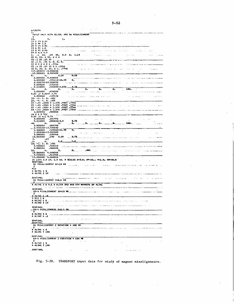
5-5Z

6118/H 1. --------------------

FJQST HAlF WITH 01,03, ANO ~MISALIGNMENT 0

1 '· '· 1.

15 1 I~ Z.S't U 2 MP 1.0 15 s 1~ z.s~ 15 6 PC 1.0 15 8 HI 2oH H0 •• 5 •• 5. lo ol 20o o05 35o Zo5 lo 1oU 22 o. 20. 0 35. 0 0 0 22 .1 -20 .• 05. 35 --22 .1 o •• 05 o. o. o. o. 22 0 0 0 0 0 1 • 77H 22 ol 20 o05 35 0 1 o77'6 22 o. zo. o. 35. 0 1 •• 77~6 -11.ooooco -o.oooooo _13. 000000 . z. 00000~ ---::----::-=-----------------------------6. "· o.to o.os

z.oooooo o.oooooo 4.000000' .JqJll0-15.45 2 • OOOC00~23.000000 3.000000 .151000

o.

_ ,.010000. o360000-4o676____loL1--~~---~----=------8. o. o. o. o. o. o.

3.000000 .050000 s.o1 .-2 5.86~5 3. 75

3.oooooo .4oq•5o 10. -2. 2. o •• 001 10. -4. 4. O •• 001 23 -.4) .0006 4 1.378 23 -.45 .0006 4 1.378 23 -,'t5 ,I)IJOi· 4 1,)11 u -.45 .ooo6 • t.H8

3.000000 .300000 _.,., o 2 o •cz 5.01 .2 4.1 '· 75

1.oooooo .ostqto

.9927 • 7746

.9927 • 7746

.9927 .1746

.9927 • 7146 ---------- --- ---

5.01oooo .rooooo-3.8 SoTS -a. o. o. o. ___ o. -- -·- o • . ----··-···-·- ---·

3.000000 .268740

- !: ~~~g~~- 13 :!~~~~~~16.-~"'s=----:o:-.----------------~-2. ooocoo-13. sooooo 3.oooooo .2oeq•o

18.000000 .280 o.oo lo olD

100.

102.

1.~: :1.· :d'o: :ocn _l._o____l.L!l----------------------,,_..;.-------3.oooooo .568•60 3o000000 .060000

10. •• ]. o._ __ .001 .. 13.000000 •• oooooo

~-::gg~~gg4:g~g~~g------------------------..... ----------24 '1214 2.5 25. loS 30. I SCAUS X•Z.St XP•25ot Y•loSt YP.JOoO­SENTINEl 01 MISAliGNME'IT SY•lO MR_ 2

FIX A AliNl 1 8

.. A AliN1 3 10 ------------------------------------

S~~T!~~~liG'II<E'IT y-;,();t-JN--------------------------------.~A~L~I~N~1-3~0~0.~1~1-A~L-:1~E~A~J~A-:O~AN~D~4~TH~HU~MB~E~R-:S-O~F~A~l~IN-1---~-------------------

--------- --------------------- ------- ---------- -----------------SENTINEl

QJ-4 I<ISALIGNIIENT 2

SY•lO fiR ___ ·-----------------------·

-}!~~~-A------------------------------------------------A ALINZ 1 8 A ALINZ 3 10

SENTINEl --~l.,._Lf!LSALl..,..:ou<L-=..._.._....__ _______________________________ _

A ALINZ 3 0 --------------------------------------------------------------A AliN2 4 .1

SENTINEl

_s~~l!~i~G;::N:;:M:::E::H:;T;---::-:ci\::O::-TA:::l;ci::O::H;-•~l::O::Q-cii:::R:----------------------------2

A AliNI 4 0 A ALIN1 1 100

-$~~~!-.~~ s.ii.-IGHMf·NT--::l---:-AO::;T;cA:-:;1:-:;I-::O-::II-•-:l:-::OcO~-:::MR:-----~----2

A Alllo2 4 0 A All"l 1 100

. SlNTIIIt~

Fig. 5-30. TRANSPORT input data for study of magnet misalignments.

0 u ,_) ,:~j • u

5-53

IHIU.l VEClOII •t..OftfO OH IEolfiiiLIMt

------ ---T~ .. ~.--~ .... ~~"--tt:-··----n::---!t::Oo:----:-::=:-----'-:~.~:~:.~·-~-:~.~:'ooo~ .. ~-J tCI .1000 0.0000 .OSOO 0~0000 o.oooo o.oooo o .. oooo 4 COl 0.0000 0.0000 0.0000 OoOOOO 0.0000 loOOOO oll46 5 Cfl olOOO 20.0000 .OSOO ts.OOOO 0 .. 0000 1.0000 ·"'" 6 lfl 0.0000 20.0000 0.0000 n.oooo , 0.0000 loOOOO oll46

·---:--o-:=--:-,.-;,:::.,~0~•!:-'!~~~:~~:"''"u'"",:-.-:c.,:::ooo--:,~ ..... =:-- ~-~soo -o:.o-·- -·--~~ ... ,::.~ •• ~---=-•• -;,:::, .. :o--::,--c ..... =c---c,:-.~n"oo::-•::-.-::,..:::-

• .061 Sll l 1 S. US U SSS SSSS UUSSSS UU UUSSSSSSSSSUSSSSS SUUUSS I SUUS SUS UUUUU I SUSUUSU SUUS USSIUSUUIUUUUS o.ooo &fill ,., Ill

.061 llfllll 16 ,.,, "

~--------·--------- ·--·---·-···- ,_.__ ~llJ....- -·-- ____. .uz ••• u ,,.,. nz " .zu eflll& '' ~· •u • .l~ 8flll1 J44 6U II .161 81111 ~ Ul M .U6 ll 16 J4J4 6 SZ 0

....... atu ___ ·-···--··---·----······-'., Ml4 tll)l..l. ··-·-·----·-·- _____________ ...o ·'"' u • ,.,.. nu o • 608 Ol 00000000 6 JU ~ 6 51 Z QQOQQQOQOQQQ ..... 01 0 • "'' 4 • 5lll 0 .uo 01 0 • )4) ~ • 'u Q • tn 01 0 6 J4J 4 6 S I l Q

:!~t-:!-oQQoOOO:- .. ---- .. --- · ·!! ::~ -··\ '·'·-~~-~----- ~o'=oo:::o~oo:::o::::oo"'o=oo .9H LZ 6 M J 4 6 I 1 J D

1.014 02 OOOQOQQO 6 14 J 4 6 I l Z QOOQQOQOOQQQ 1.0., 02 0 • " J 4 • ' 1 z 1 .. U6 02 OOOOQOQO . " 4 J 4 6 S OlOUOOOOOOO

{:ill-~~- --:!-- .. - ·: ~ : ·: -,-'·-~.-','-----~ l.JJilJ ,, 4) 4 ,, 11 lol'f'9LJ 61 4) 4 61 II 1.460 u ,, ~ J " • ' 1 l 1.120 LJ " 4 J 6 S l II D laSU U _____________ ... ______ ---· . ------. 41_ . 'll .... _ A.S. ____ ...L..l.l ___ ___o 1 .. 642 SE"l WWVVWWWWVWWWWWWWIIIWWWWWWWWWVWWWIII62J 14 1 6 S 1 28WWWW t.ros "'"' hS ,.. s • s 1 ze lol64 SH1 161 J4 J 6 S 1 II

•• us ""' 165 )4 ' • ' 1 ,. l.IU SE"1 , 161 )4 I 6 S 1 ze .la9~6 . .K.f.l... __ _ . . . .... . 16J . MJ 6 S. l.D ·---~ ,2 .. 001 Sf"1 WWWWWWWIIIWWWWIIAIWWWW"WIIfliiWWWWWWWWti16U )4) 61 1 21tfWWW 1.061 SE .. Z WWWWW'IIWWWWWWWWWWWIIWWWWVWWWWWWW1621 )4J 61 l 28WWWWW 2.12• SE"2 1 n 411 , s 1 n 2.11'9 SEP2 1 6 5 411 6 I 1 2.1 2.250 SEP2 1 6 S 1411 6 I 1 28 z.tu. n~.z. __ . 1 •. ' • n • s... .l...n __ 2.n2 "''"' 1 • ' 4 n • s 1 21 2.4)) SH2 1 6 I 4 IJ 6 I 1 Z1 lo4'fJ Sf'l wwwwwwwwwwwww~wwwwwwwtotWWWW1 6 S 41 U 6 1 U llfW...,.,.. 2o554 S( .. J WWWWWWWWVWWWWWWWVWWWWWWIIfWWWW11fWW1 16 5 4) I) 6 I lJ 8~ l.61S SHJ 1 l6 I 4 J IS 6 S U I z..tl6. UtJ I Z 6 t 4 I U 6 S. __ U.L ____ _ 2.n1 UPJ 1 z 6 s • s u • s u • 2.l'fl SE"l 1 2 6 5 4 J ll 61 ll I 2.UI SEPJ 1 l 6 S 4 J 1J 61 U I 2 .9U SEfiJ WWWWW"W"WWWWIAIIIIWWWWWWWWWWWWWWWWWWWl l 6 S 4 J IJ 61 ll IWIIIIWIIfWW 2.910 Sf"4 WWWWIII'IIWWWWWWWWWWW"WWWVIIIWWWVWVWWl 2 6 14 ) IJ 65 12 IWWWW J.04l SEP4 l 2 6 S J 1J 65 U.,e J.IOZ Sf"4 l 2 6 41 J 1J 61 U I )oi6J: SfP4 1 2 6 !i J IJ 61 12 I J.2U SfP4 1 2 46 5 J 1J " ll I J.2e• SEfl4 l 2 4 6 SJ 1J 65 ll I J.l-45 SEP4 w..-WWIIIWWWW-IIIWIIVWWWWWWWWVWWWWWWWVWW1 l 4 6 5 J 65 II IWW"""* J.-\.ll6.. u ____ 1 z 4 • -n J iU u a .. _A

'·"" u 1 z • • ) ' , " 11 ' 0 J.sn u 1 z 4 •• u ., u • o ,., .. u 1 4 • ' • ll • 0 Jw64~ L4 l 42 6 U 6 ll 8 0 J.l'lO OJ 00000000 II 42 )65 J 4 61 UOfiQOQOOQOCIQ 1.111. -'ll.. _____ .Q _ _ . u" z J 56 J 4 . 65. .... u..a ... ________ _ ).Ill ~~ ~ 81 4 l n 6) 4 6 2 I G s.n2 OJ QQQQQOOO 114 2 s ., " z 1 QQGQOOQOGOGQ ) •• , a. OOOQQOOQ 14 2 ' 6 • ., ll • OOOOOQQQGOQQ •• oH 04 o •• 2 " • 4 z 1 o •.on 04o o 14 1 s 1 6J • • z 1 o .hll"--''i..~-------·- . - U... l. , l • J ... . ...... 6.5. ___ ...z....a... ·-·---- ---------~ 4.l'f6 t..e •II 2 5 J 6 J 4 6 l I 0 4.251 L6 ... l 5 J 6 IJ 4 6 2 I 0 •.Jll L6 4 I l 'I J 6 11 4 6 l I 0 •• sn u • 11 2 s J • 11 4 • z • o 4.440 11112 4 II l J J 6 1J 4 56 ll I Ill .i.o..1.0A....I..I!I..Z.. _________________ t.._u___ 1. 5. ,. IJ "' .... .z..a a. 4.561 11112 4 II 2 S )6 IJ 6 ll I Ill 4o6U 8112 4 11 I J 6 1J 16 l I Ill 4.UJ P2 4 11 l I 6 IJ 6 21 I Ill •·'"" e•2 4 u zs ,, u " u • 111 4.105 U2 4 Ill 5 6) IJ 4 56 2 I "

~-....1.1._.1.. _6__ 1. ... U _ .-to ...51 .1.1. .. II_... ------A •-•26 t.. 1 • ea ' z ' J n " z 1 o 4w91l ll 4 II I 2 6 ) IJ M4 11 I 0 5.041 SEX1 nuu 4 II !i 26 J I 16 4 ll I U.l.lJli.JlUJlU Sw109 SUl Jl 4 IU 26 J t t 41 I I. 1.14' SEIIl Jl 4 15 6 J 6SJ 24 I I.

:.~!~ :::~ ••u•: ~-}--{-~"t.···-·ea______ ·--~u"'a-u"'u"'a"'u"'u"'" ,.,,, ll ' ••• 2 J 211 614 • 0 5.41) ll . 4 5 61 l I UJ 645 I D s.•u St.ITJ sussnnsussussuussssssssnsssnssss 1 sssssssssssssssssssssssssnssussssssssusssssss '·"'" .... . 4 ' ... l ' 11Jl ... ' • 0

So6M \.~ S.lUU

'·''' l~ ,_.,. t..•

U I Ul + " I

•' • e& n tJ&z• ''' "'' e&JIJ u• •se

o • .. : • • '!, !a: : '!~a • !:, S 6 •U I J 4 1 J 6 I 1M AI Z

s.uo U I 6 IJZI J 4 1 l 16 I 6.0ll UO I 6 lll J 4 l l 16 S 6.011 Lll 16 " l Jl J 4 I J I 6 S

--------·-----~--·---·---·-----------------~·

0 • 0 0 0

4.tooo J.noo s.oooo 2.2100 1.1000 .tsoo o.o .noo a.toOO z.zsoo ).0000 J.noo ... ,.

MJI;Il tU• VliU Ill• ..... (OIUtKTIOttS

yn!ICAL lfU ttQ!IllWIAL y .. • 0750 Clt• .UOO Ul• .U~ t41• .1000 fll• .JlSO 161• .4500 Cll• olltO fll• .6000 191• o6l10 oOlJO Cll• .UOO Ul• .zzso 141• .)000 CSI• .Jl50 C61• o•UOO Ctt• .szto Cll• •6000 ttl• .etfO

Fig. 5-31. Beam line graph for example 6.

5-54

y'(mr)

-1.5

-24

Fig. 5-32. Vertical phase space showing effect of the misalignment of quadru­poles Ql and Q3-Q4. A) No misalignment of any quadrupole&, B) Ql misaligned by 6y' = 10 mr, C) Ql misaligned by 6y=O.l inch, D) Q3-Q4 misaligned by 6y' = 10 mr, E) separated vectors with no misalignments, and F) non-separated vectors with no misalignments.

__ y_PfiO_N _3 i;:_AR.Cti (;

13 2 13 2 1 1 10 1 10 Q 0 9.~ 13 2

·-------~ ... ~'" - --- ····-- ... ·-· -- ..... .

5.02 .7; 7.5 5 3 • 375 5.01 1.; -7.5 5 3 • 375 5.02 .7, 7.5 5.

---- .. h ... ~-·-2~-10 2 1 o • a 1 10 't 3 l • 0 1 13 1 :iENTINEL OPT ION 3 iEARCH Crli-TAtiL~ VA~IABLES 1 ANO 2 _;} ________ ···•· ................. ··--··-··· ···-············ -. ····•··· -·-·· . 1 5 10 1 il 10 2 -'+ -11 -2

SENTINEL

Fig. 5-33. TRANSPORT input data for det~rmining complete set of waist to waist transfers. Option 3 must be used to step over the separatrices in the multi­dimensional chi-square space.

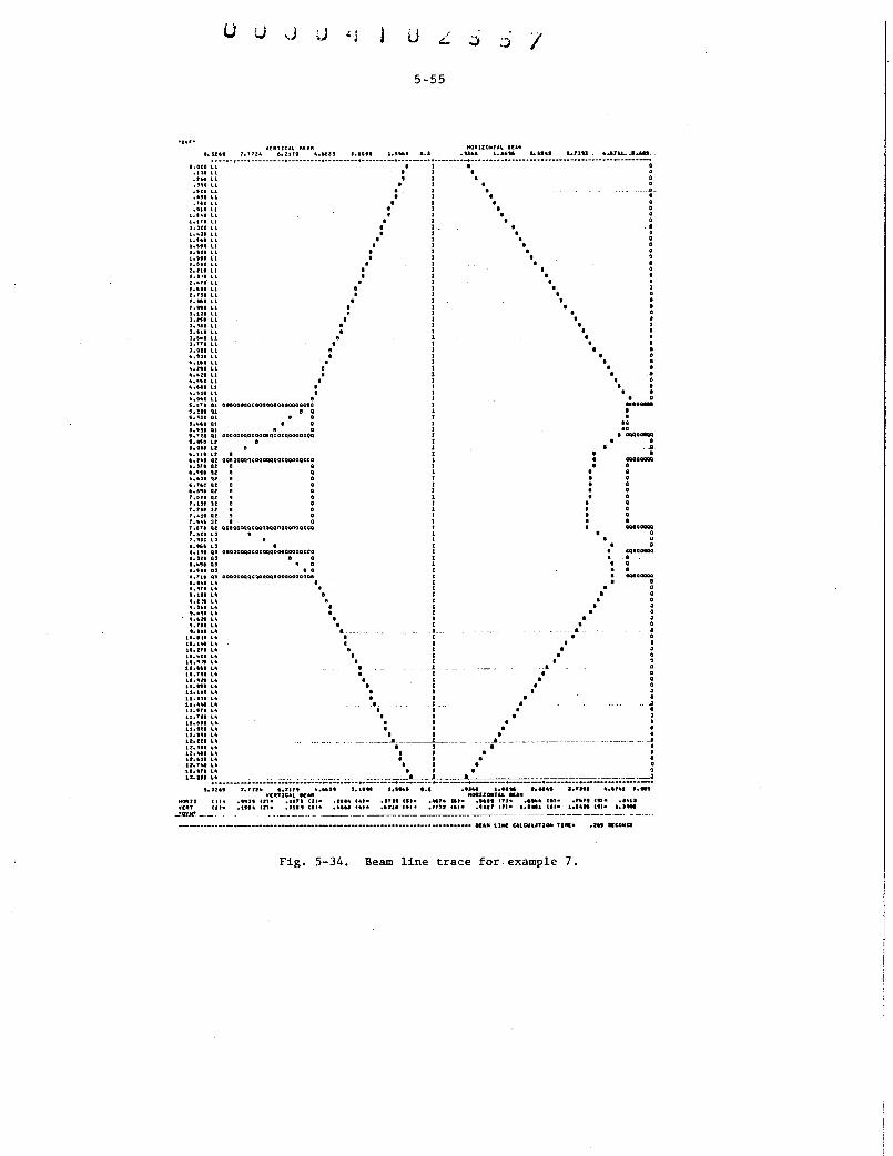
u u I 5-55

V(IHJC.Il 8Ufl HOII:UOtlfU. IUfl 7,7rll<o floZI19 lo.IUlJ< J.UU l.UUi .1.1 .uu LUU Llld a .. uu ~..a.r.u __ ,_.... ·-------·-·---------·---------·---------·---------·--------··----·---·----·---··---------·----·----·---------·------·

loOGOLI I I I 0 dJI L1 I I I 0 oU.f ll t I I 0 .no Lt t 1 a o otU ll I I I ... .a_ oUI ll I I I 0 .reo Lt 1 1 1 o o'lll lt I I I 0

lolliOlt I I I 0 loll't ll I I I 0 loJIO l1 I I . I D t,.,JO ll I J I 0 ••• 61 ll I I I 0 t.Ut lt I I I 0 lotn Ll I 1 I 0 Iotti l"t I t I 0 z.oeo Lt 1 1 1 o t,ltO L1 I 1 I 0 ZoJII ll I 1 I 0 z,uo" l1 I I I D z.•ao u • 1 • .;, z.ru Lt e 1 1 o z.t61 1..1 e t 1 o t.tu U t I I 0 JoUI lt I J I 0 J,ZU Ll I I I ,) lo1U l1 I I I D 1.111 ll I I I il J,t.l!l ll I 1 I 0 J,711ll I I I G 1.911 lt I I I D 41 0 "1!1 lt I I I 0 .,,tU Ll I I I D ... ztt lt II 1 I 0 ... 41lt l1 I 1 I 0 lt,'IU ll I I I 0 loo6U U I J I I ... ut Lt e t 1 o to,9.,0 Lt I I I 0 5,071 Qt OOOOQOQQC!10QOQQOOQOQQQ080 I •ao-'•!lt 'lt I Q I I t.uc 01 0 I I •·••tot o 1 10 t.no 01 1 o 1 u 9o1U lU OOOQOOQOOOOQIQOOOQOOOOOOQ I I OQQOOIQQ '•"0 t.l I 1 0 1 0 911 Lf 1 . .JI loUI Ll I I I 0 6,l'G Ql OOtiQOOQ1COQQQQOOCOQOOQOCQ I I CIOQQOOIQ loS'fl O:l I Q I I 0 6.'1U U I Q I I 0 6 0 UO 1l I 0 I I 0 •·:r•e u e o 1 1 a 6.1'11Ql I 0 1 I 0 1,Dllt QZ 4 0 1 I 0 r.ut u e o 1 • o r.ut u a o 1 • a 1o410 Ql '!I 0 I I 0 1,'!1fiG :U I 0 1 I 0 1,611 Ql QOIQQOQQC:QQQQQOOOOOO?OtCO 1 I OQOOOOIIQ r.ua LJ • 1 o r .u~ L s 1 • g t.t61 Ll I 1 I 0 1.191 lUI OIOQOOQQC:OOQQQ00800000CC:O I I "'OOOOIN Iolli QJ I Q 1 I 0 .... sen o 1 eo lotiO QJ I 0 I I 0 lo111 Q, OOQQQOQQClOQOQOOo<IQQQQ108 I OQQQOOQQ t.tet~ Lit I I 0

'·'" L~~o e 1 • o Iolii Lit I 1 I Q

t.l!t Lfl I I I 0 t. 161 Lit I I I tolt'tl L• I 1 I toUI Lit I 1 I t.nl Lit I 1 I toltl Lit &. --· .J.... 8

UoiU Llo I I I Uoletl Lit I! 1 I U.lU Lit I 1 I u.~ooe L~t 1 1 • Uo'l~ L• 8 I I 10o661 Llo I . 1 . . .& ... , .. lllo • 1 • Uotll Llo I I I Uoltl Lit I I I u.ue Llo 1 1 1 lloJtl L.. I 1 I U.o"-' Llo .I. .. J --- I .. .II 11.'111 Llo I I I 0 Ho111 llo I 1 I 0 u.UI L.. I 1 I 0 llot61 L• I I I 0 Uol91 Lit I I I 0 UoUI Llll -·---•-------.....L_·------·-·..1.--- ..... - .. ·---·-·- _JI llo 151 L• I J I 0 Uololl Lit I I I 0 U.6U Llo I 1 I 0 u.r ... Lit I I I 0 .,,.,, Lfl I 1 I 0

&s.an ~! ........ --+----~:.:;.-:.. .. :. .. :.:.;.::. .. ·.:;;.~:..: .. .:.;.:..~.-.. -:-:::: ....... - ............... t--.---.-.. -.• .• ,----,-----.:~;:~~:::;.;::..~-:---.:.:= ... :.-~ MOitU ttl• Yt:ltT Ut•

~--·-

'· rn.. 6ott1t ....... Jolltt YI.TICAL Mlll

oltll frt• ollfl Ul• olllfl Cflt• .ut~t crt• .aut ut• ·••u hi•

....... ••• ..,... ...... lollltt '·"" ltotru .... , MOIUZOIIUL lUll

olflt Ctt• .flilrfl elf• ol6tt trt• •• ~It eel• .r .. rt CW• oi"'U oiUI ttl• ,rrft C61• otltr trl• a.t .. l Cll• lolloM 1•1• lol ....

·--------------·--•·•••••·-··-··--···-·--·-----·-···-··••···-·-·~·- et•• \lM: C&LC:U'-'flO.. fltC• oiW KCO•CIS

Fig. 5-34. Beam line trace for.example 7.

5-56

K',y 1 (mR)

I 2 Vertical phose space ( V PS) Runs I, 4, and 8

Horizontal phase space ( HPS) Runs 2' 7 and 8

Run 4

Run 2 and 3

H PS Run I and 3

12 K,y(cm)

XBL752-2264

Fig. 5-35. Eigen-ellipse for the solutions of waist to waist transformations of the symmetric triplet lense of example 7. The quadrupole excitations are given for the various runs shown in Table 17.

/

0 (J _., .. ,

5-57

I BRF&~ UP CROWE liN( FOR USE WITH I~PUTED H ElEMENT IN SECQIIfD ORDER BAEO-CROWE BE&MliNf AT lfP-lASl CHANNEl 0

15 0 I 22 OR7 22 OR5 1. 22 .05 0 1.0~ 22 0 40 0 llv 1.o .o5 •o.o 1.06 uo.o o.o 2.eo o.2 BEA"l. -13 2 S 10FF l] 2 16. 29. -1. v•R•IT 24 o 30 30 o I 6 24 I -.05 .05 -1.06 1.06 I TARGET Sllf 24 4 .18 .22 .01 I E SPECTRUM

~:oo 0 ·~~51 °1-2.58358 to.l6-cil-- -----· ·-------·-··- -- --·-------·---------

3. o. 35 SEPl 5.00 0.7 1.54221 .... oz 6 0 I 1 UPOATE 3· 0.55 02 16 .. 25 }6. 5. 7.62 GAP 16. 7. .Z6 FRINl 16. 8. 4.4 FaiH2 16. 12. 0.5109 Rl 16. 13. -. 7871 PZ ~6 3~1 0z P;RI4. l. &NGlE ... N. ____ _

4 1 60 0 'ENOl 2 30 0 PFRll ). 1.~ 0) 16. 12. 1.2692 Rl 1~. 13 •• •nz R4 2 -lO 0 PFOZ 4 1 -60 0 RENOZ Z -)0 0 PFR22

1. .65 Olt 13. 4. 14T Xl

---·-·---.. - -- ··-·

13. 42. I PRI~T T. MATRIX. 1CIE.GTE0 __ 8Y .. r.t:tE_$1G.MA _MAn IX VAlUES __ ----- ----·-·----3. e65 Olt

16. 12 •• 9772 R4 16. 13. 1.2692 R3 2 -)0 0 PFR22 4 1 -60 0 HN03 2 -30 0 PFP2 ) • 1. 6 03 16. 12. -.7871 RZ 16. 13. 0.5109 R1 2 30 0 FFR11 4 1 60 0 8EN04 2 30 0 PHI 3. 0.5, 02 l] 1 134 13 42

5 .1 1.U~ 1• OJ '· o.~s SEPl

----------------------------···--

s .n -1.o•u 10.16 o• l.2 , . ' 6 4 2 4 CHAMBR I CHAMBER HERE -P 2.0CM IY -•• CM 131 1)4 U-42 ., ·' . l 2

----~------ ---- -----·---- -- --·--

5 .5 1.6215 10 OS 3 .25 5 .s -1.6601 10 06 3 1 ) 1 ) .3 1 l T2 TARGET 2.1 X •• 1 CM fUll SUI 6 4 2.05 1.35 lT2

l T2 TARGET HERE S l~CE TR&NSPOR T

I X•-• 2.05 CM 1). -42. I PRI~T

1). 4. "4TXE 3 .43 EKTRA 3 .1 flTPA SfNTI~il

2~7 X 4.1 CM FUll SIZE IS IN OEVEASEO PlANE.··-- ..... -· ---···--·-.

V•-•1.35 CM T MATRIX WlfGHTED 8Y THE SIGMA MAUIX

Fig. 5-36. Transport input data for example 8.

5-58

INITIL VfCTO• ll'lOTffO ON IIEA"liNf 1 Ul 0~0000 Q,OODO 0.0000 0.0000 0.0000 l lfll o.oooo 0.0000 o.oooo o.oooo o.oooo :s ttl .o~oo o.oooo 1.0600 -o.oooo -o.oooo 4 401 0.0000 "O.OOOQ 0,0000 110.0000 -0.0000

YHtiCAL I!(A,_ HOII.IlONUl 1(1. ..

o.oooo t.oooo

-o.oooo -o.oooo

o.oooo ·-o.oooo -o.oooo -o.oooo

,,oooo zo.oooo .,.aooo to.oooo ,,oooo o.o •.oooo 1o.oooo u.oooo zo.oooo n.oooo Jo.ooo ·---------·--------.-·--------·---------·------·------·--------·---------·---------·---------·-.. ------·--------o.ooo 01 ' " 0

.2:)41 01 ' ]4 0

.41.11 01 J ) " 0

.TO! 01 J ) 0 •• Jl 01 OOOOOOOOOOOOOOQOOOOOOOOOOOOOOOOOQOOOO ) J OOQQQOOOOOOOOOOOOOOQQOQQQOOOOOOOOOOOOOOOO

1.1 Tl 01 OOOOOOOOOOOOOQOOOOOOQQOOOOOOOOOOOOOOO " J J OOOOOQOOOOOOOOOOOOOQOOOOOOOOOOOOOOOOOOOOO 1,40, \EPI U 0 1.61'1 Ol OOOOOOOOOOOOOQQOQOOOOOOOOOOOOO " J OOOQOOOOOOOQOOOOOOOOOOOOOOOQOOOOO t.lh 02 0 ~~ 3l 0 2.101 02 QOOOOOOOOQOOOOOOOOOOOQQQQQQQOO I~ J J ~ OOOQOOOOOQ\/OOOOOOOOOOOOOQOOOOOOQQ 2.1~2 02 ~ J J .. 0 2.5T6 02 ,.. 1 , 0

2.110 02 '" J , to 0 J.Oto5 lfHOl 1111111111111'11111111'11'11111""111'11111111'111111111'1111111111111MIIIII .... MMIIIIIIIII'IIWtllllll'l I to J ) 4 111111111111114111111114111 J.2T'f llfNDI Ill J J to ).51) '\fNOl 1'1 I to J 1 tofl J.7toT 1£"101 IIINIIIII'IIIIIII111111111111111414141'111111111110111111111MI'IIIIIIIIIIMIIIIIIIIIIIIIIIMIIIIIIIIIIIIIII (I 4 J 1 to 1.<~11 01 I 4 ll 41 to.lt6 OJ e H 1 2 to e to.toso n1 e 1 to 12 • e to.6eto os e s toJ 2 " e to.<~u 01 e 1 -s 2 4 e s.ts2 OJ 11 J4 1 2 e s.sn os a toJ 1 2 to a 5.621 IEN02 .. lllliiiiiiiiiiii"IIII'IIII""'I'IIIIIIIIIIIIIM'"IIIIIItiiiii'IIIIIIIIIII'IIIIMIIII4111f'llll'lllllllll I to ) 2) 2 to a '·"' flflrC02 111 e 4 1 n 2to e 6.01!1'1 IIEN02 Ill 14 )lJ 4 II 6.12) llofN02 l'tiiiiiii4111111111111111111111UIIIIMIIIOIIIIIIIIIIIIIIIIIIItllllllllllllll111141111111-lllllllllll lito )) to2 1!1 6.551 04 lito 12M 2 e 6.T<J2 04 U J lto 2 II T.o2• 04 u 1 2to 2 e T.l60 04 II 4 J 214 2 II 'f.U4 04 e 4 J lJ 42 e 'f.U'f 04 II 4 J 2J 4 II To'I6J llfNO) Mlllt11411111!UIIIIIIIIIIII'IIIIIIIMMIII.IIII'III""'III•I'I-IIIIIIIIMIIIIIII'IIlllllll- II to) 2) 24 I l.l'IT llffiiOJ Ill II 4 21 2 4 I 1.411 lfHOJ Ill II )4 2J l I I .665 11010) IIIMitMMIIIIII .. IIIIM-·111111111"'"'""0101111111111111-MOIIIIIIIIII-MIIIIIIM IJ 21 l II 1.'100 OJ II J 4 Z1 2 4 II '1.114 o1 e J ., z 4 e •• :ue 01 e s 4 2u to 11 •• 602 01 a J4 u2 toe •• 1)6 OJ A 4) U 411

tO.Ofl OJ I 4 I 21 6 tO.J05 OJ _. 1 21 84 lQ.)J'f 11£H0to IIIIIIIIIIIIMMI41411111111111111111111111111'11'1"'1MI1U"III-,.MI'I•III .. ICIII'"IIIJIIIIIItlll ) 2J flto to. Tn flfND4 • to J 21 114 ll.OOT lffll~ 1111 4 JlJ lito

"'1"111141111111'111111111'tlll D .. D D D D D

111111111111111111111'11111MIIII­D D D D . • """""'1111-111111111'1111 . .

llllll'l_lt_llll'llllllll . . • D . • .

11.2to2 fii'NOt. IUIIIIIIIIIIIIII"* .... M111111""11111111111111111111111MMIIIMIIIM1111-IIIIIIMIII•IIIM to )) "4 111'1-IIII'IOCM"''I'I-ll.H6 02 4 JlJ 84 0 u. 110 02 &4 ) l1 84 0 ll.llltoto OJ OQOOOOCIOOOOOOOINOOOOOOOOOOOOOO 114 J 2J fltoOQQOQOOOOOOOQqOQOOQOOOOOOOOOOOOOO u.na OJ o eto J ll e• o u.tou oJ oooooooooooooooooooooooooooooo e " J 21 ooooooooooooooooooooooooooooooooo U.6 .. 'f SEPt fl 4 J lJ 0 u.eu SEI'l s l1 eto o 1J.l15 04 0000000000000000000000000000000000000 11 to J 2J 11to OOQOOOOOOOOQOOQOQOOOOOOOOOOOOOQOOOOOOOOOO lJ. H9 Oto OOOOOOOQOOOOOOOOOOOOOOOOOOOOQOOQOQOOO fl ,_ J lJ "to OOOOOOOOOOOOOOOOOOOOOQOOOOQOOOOOOOOQOOOOO 1).511to l1 fl to J 21 11to D u.ue u a 4 J u u o lto.052 ll 1'1 to) u fl4 0 lto.lt6 l1 8 to 2J eto 0 14.510 l1 8 4 2J 114 0 tto. TH ll 8 J 4 21 h 0 lto.911'9 l1 • ) 4 J 84 0 t5.UJ u e 1 4 , '" o u.ton ll II) 4 J 114 0 u.ut Ll e J 4 Jllto o U.'l26 l2 I!) 4Jto . o t5. on• CH&Mu sssssns sss sss ssssssss sssss s ssu ssssssss ssssss t sssss ssssss ssssss sssss sssssss ss ssssssss ss ssss ss sss sss ss ss 16.160 l) u tol 0 U.J94 lJ fl) 4h 0 t6.6211 LJ n to s2to o 16.162 l4 tl ' to Jl 4 0 u.on Lto e ' 4 .u to o u.JJt L4 e Jto u 4 o n.,., Lto e toJ 12 4 o n.'fn L4 e 4 s u 4 o u.on L4 e J u to o 11.268 l4 e 4 1 12 4 o u.502 L4 e 4 1 n 4 o ••· TJ6 Lto e to ' u 4 o U.'l'fO 05 OOOOOOOOOOQOOOOOOOOOOOOOOOOOOOOOOQQOOI 4 J JZ 4 00000000000000000000000000000000000000000 1•·204 05 OOOOOOOOOOOOOQOOOOOOOOOOQQ000000Qe0040 J J2 4 00000000000000000000000000000000000000000 u.tol9 l5 fl to ) )2 0 1 'I .6 TJ 06 00000000000000000000000008040000000000 J J2 OOOOOOOOOQQOOQOQQOOOOOOOOOOOOOOOOOOOQOOOO t•.'90f 06 OOQOOOOOOOOOOOOOOOOOQOOfi00400000CJOOOOO J Jl OOOOOOOOOOOOOOOOOOOQOQQQOOOOOOOOOQOQOOOOO JO.Ul l6 8 to J Jl 0 20.JT1 u e 4 J 12 4 o 20.610 l6 ) 12 4 0

· zo.u• L6 • 4 J n 4 o ll.Ol't l6 8 4 J 2M 0 zt.JU Ll J ZM 0 U.546 lf )24 0 21.111 Ll 14 J24 0 U.OU Lf 8 4 J 4J 0 u.zu ll IIJ ,.., 0 u .u• L u uusssssnssssss sssssssnsssssssssssssssssssss sssssss 1 s sssssssss suss ssssusssusssssssssssss sssssssssss sssssss llotoiJ EI.TAA J 4 24 0 U.Ttf UTU II J4 24 0 U.'IJZ fiTaA I 4) lM 0 ZJ.1116 (IUA I 4 1 2114 0

tJ.HD !~!-~:..._:,;.__•----:..•-----•---•-!_~--!---..!!!~---•-=------------•-----------•-----: Jo.oooo 2o.oooo n.oooo 1o.oooo 5.oooo o.o , .. oooo ao.oooo u.oooo zo.oooo n.oooo 1o.ooo

VERTICAL llfUI MOI.UONlAI. IEAIII MJIIt Ill• .5000 121• l.OCKKI 111• 1.5000 141• 2o0000 IJI• 2.5000 161• J.OOOO Ill• ).~0 (II• 4.0000 I'll• 4.5000 VUT Ill• .5000 Ill• 1.0000 Ill• l.JOOO ltot• 2.0000 Ul• 2.5000 161• 1.0000 Ill• J.5000 Ill• 4.0000 l'fl• 4.5000 ..., ... -------------------------------------------------- 8EAIII lilliE C&LCUUfiON Tlllllf• .502 SECCWCOS

Fig. 5-37. Beam line graph for the LEP channel. Note the use of the vectors for determining the beam spread produced by a momentum deviation and determining the locations of waists by displaying the points of phase reversal.

u J J ~ .. ,· ·-5-59

8EAR-CROwE BEAMLI~E WITH 25 ElEMNf INPUT Of 8ENOING MAGNETS IN 2-NO ORDER 0 15 0 I I

~ 2 .~~\o 1.06 110 0 2.8 .2 · · --------- · · ·---· ---------------------17 I] 2 Z4 o 3o 3o o 1 6 l .62 5 .51 -2.58358 10.16 3 • 35 5 o 7 lo5H21 14 I] 1 16 17 9.6 25 ••G-ETS 52 12345 1 • aqoa o:;)" o 1 0~4

0 0 .9Qc;Q .0004 0 0 0 0 -4.835 .9990 0 0 000010 -.1811 -.IH5 -.03256 0 0 .09842 0 0 -1.707£-2 2.669£-3 OR5

--- :...4o67 __ ;~~~ 3~.~a~:~ 7o0o 0.~9~~9~9 ~ -.oz9z9 .oo6o2e o•' -1.&,.;-_;ezo9 Oit-1--=z:z-;-,------o•J .oznz .-oo6qz o -.01206 -.oo537 OR9 .09951 -.0409'1 o o OR) oZ519 ,JJZZ 0 o029ZZ o01711 009 lo6!7 o09951 0 0 .09162 .08065 .01844 0 0 -.1032 0 0 .009997 -.002065

!) 1 13 8 .13 42 13 48

o•5 o4434 .1967 0R3 .3996 l Tl5oJo~l

5 .7 1.1244 14 3 .35 5 o51 -1.0613 10o16 3 2 3 .7 6 4 2 4 13 1 !) 42 3 • 7 ] 2 5 .5 1.6215 10 3 .25 5 .5 -1.6608 10 3 1 ] 1 3 • ) 6 4 2.05 1,35 LT2 1J I 1] 42 SENTINEl

---------

-----------

Fig. 5~38. Transport input for the same beam line of Figure 5-36 where the bending magnet systems has been replaced by its first and second order trans­formation matrix.

OATE•61211T4

BEAR-CQOWF. 8E.t.Ml1Nf WI fH 2S ELE•NT INPUT OF 8ENOING MAGNETS IN IIU~ITI I 15.0 51VfCI I 22.000000

7t f\EAII(l I 15c sec 1 1 191101 I 211 PLOT! I BCll I 30C01 I HIL2 I 36102 I 401102 I "ZillA! I 45C~Afl I 491103 I H1104 I 531 105 I 551106 I 57103 I 6lfl3 I 63(04 J 67Cl4 I 691L5 I 711 SLIT! I 751 107 I . 771108 I 70(l6 I 8IIL7 I 83105 I 87CL8 I 89C06 I 9)( l9 951 LIO CJTCLll 991L TZ

IOH 109 ----1051 1010

22.000000 1.000000

17.000000 13.000000 24.000000

3. 000000 s.oooooo ) • 000000 5.000000

13.000000 16.000000

25.0 13.000000 13.000000 13.000000 13.000000

5.000000 3. 000"00 5.000000 3.000000 3.000000 6.000'JOO

13.000000 1 ).0001)00 3. 000000 ),UOOJOO 5.000000 3.000000 5. 000000 3. 000000 3.000000 3.000000 6.000000

13.000000 ··13.000000

o.o 1.0 1.0 1.000000

o.oooooo .osaooo

-0.000000 2.000000

0.000000 40.000000 -o. oooooo

o.oooooo 1.060000

-o.oooooo

o. oooooo ·· · 3o. oooooo 3o.oooooo .620000 .510000 -2.583580 10.160000 • 350000 .7ooooo

1.000000 17.000000

MAGNET ·t.oooooo 8.000000

42.00001)0 48.000000

. • 700000 .!50000

1-542210 H.oooooo

9.600000 52.0 12345.0

1.1H400 14.000000 .

.510000 -1.061300 10.160000 2.000000

.700000 t..oooooo 1.000000

.. 2.000000 • 700000

2.000000 .500000. .250000 .50JOOO

1.000000 1.000000

.300000 4.000000 1.000000

42.000000

2.000000 4.000000.

1.621500 10.000000

-1.660800

2.050000 1.350000

2-ND OkDER

o.oooooo uo.oooooo

o.oooooo o.oooooo

o.oooooo-1~-oooooo

o.oooooo 2.aooooo

6.000000

CASE NUMeEII 4- Q-F

o.oooooo .zooooo

Fig. 5-39. Transport data array for data input of Figure 5-38.

5-60 .HIS TCGA..t.MS

• 22 --03 .03 .015 -H 2~ 8 -12J4l. -.6 .. 6 .6 -60 60 20 24 12 24 34 2" 13 24 I 24 2 24 3

~· ~LUS 1.0 PERCENT "O"ENTU~-----··---------------------------22 OR5 I• 0. 22 -.o3 .o3 .015 -z~. 24 a -12341. -.6 .6 .6 -60 60 20 2~ 12 2~ I) I '-PWS 1.0 PERCENT liQf'EN"rlilllt-·---··----·-·-·-----·--~--------------

22 OP5 -1 22 -.03 .03 .015 -24 24 8 .;12HI -.6 .6 .6 -60 60 20 24 12 24 13 ELLIPSE 0.05 40 !.06 110.0 24 I 24 2 24 3 2'>4 24 13 24 12 24 H

1000 -12141 S X-XP-Y-YP RANDO~ 80UNOARY 1000 POINTS

ELLIPSE 0.05 40.0 500 -121 S X-XP RANDOM BOUNDARY 500 POINTS 24 1 242 24 12

SENTI NFL

Fig. 5-40. Data input for TRANSPORT to calculate particle histograms and scatter.plots shown in Figures 5-41, 42, and 43.

PUHE• l] NUMBU OF POINTS• 1]5 1------1------1------1----1------1------1-------·-----1--------1-----1

1.ZTOE>OO • • ---~:m~=~~ -----.- ---·-- -----

-l.ll9E+OO 1. 069E +00 t 1.019E+OO t 9.690E-Ol t 'i.,l89f-Ol t 8.668E·Ol a.taTE-ol T.686E-Ol T.I85E•Ol 6.6HE-Ol'

11 11

1 2 ________ ..... 1

~:!:~~=~~ : · _____ _ 5.180E·Ol t 4.679E·Ol t 4.!18E·Ol 3.677E·Ol '!.176E-Ol 2. 615E-Ol 2.1 74E·Ol 1.673E·Ol

]

1

1 1

11 1 12

1

... . . ....... ·------------··-- -·· .... -•

1 l 1 1 1 u .11

1 l 2 11 ll 12 l 1 1 1 1 l'111ll +1

12 I 1 2 t11U

11 1

II 21U t1212112 ...... 1.2. ________ _ I 1 1 2 Ill 2 .1 1 I 1

2 II 11 t 211 12 1 1 11 2 1 It 113 12 1 2 12 1 2 2 1 2 •2 1 1222 1 1 11 11 1

11 I 2 1 1 l 1 Ill 222 1. 111 3 1 24 2 1 I 12 2 J2 1 II t 2 121 11 I 1 i .2 I I 1 12t l 212 21 2 1 2 111 1

1 211 1 I 1221 2 1 2 1 1 2 1 1 I I 21 1 Ill 1 1

1 I

.1.

1 1 1

1.

i.I71E·OI 6. 704E·02 lo692E·02

• 1 ' 13 2 1211 21111213 11 1 1 t

·3.31QE-02 -8.3lOE·02 ·1.3HE-Ol ·1.8l5E·Ol -2.33oE•OI

!=-:_-,:=!.==--,-==--'=-=-~-:-:::-•~:,-~-•----llfi' 2~i-;;~~f~~~4;-;-;•-;~i 1 ~-;•;·:-:-~i""'--.,..--,,.--: • 12 1 12111 2 1112 11 t I 2 11 1 II 11 411 I 2 11 1

11 1 11 -2.837E·OI

~3. ))q£-01 --------------------

-~. 940E·OI t -4.HIE-OI •4. 842E-Ol -5. J43E•Ol -5.844E·Ol -6. H5E-Ol ·6. 846E·Ol

l 1

11 1 1 1

1 1 112 II I 1 311 I Ill 1 1 1 21+1111 1 1 1 I 1 221

1 1 1 2•21 1232211 3 1 • 11 1 2 111 1 1 1 1

1 2t2 11 11 I HI 11 2

1 1

11 2 2 Ill 1 I 1 11 11 1 11 121 2 11511 I I

1 11 11 2 t I 311112 1 1 1 1 Z 1 1 11 1 1 I 11 11 . 1. 1 1 1 Z t 121 1 1 I i ..L .. _ ----.. - ·- ·-·-------·-·-

1 Ill 1 2 Ill 1 1 11 1 1 1

111'1 111 21 2 211 til 11 11 1 11

11 I 1 • -T.l47E·OI t ·7 .84QE-Ol ·8.350E-Ol ·8.851E-OI

11 1 ti'' z 1 11

1 • ·- __ __J __________ --- --------- .• -9.352E-Ol -9.853E·OI •l.OHE+OO -l.OR6E+OO t -l.l36E+OO t

1 1

111 1 I

-l.l86E+OO t t -1.236£+00 ... ---------- ---------- ,- _ .. ________________________________ t

l-----1------1-----1----1------1------1------l-------·-------·-------1 ·5.22E-Ol ·.4.14£·01 -3.06E-01 ·1.97E-Ol •8.85E•02 1.99E·02 1.28E-Ol 2.3TE-Ol ].4H-Ol 4o54E·Ol 5.62E·Ol

111• 14 1

• o&o• t2t• .0)25 • .,) • .OS42 161• .0651 ClJ• .0759 C81• .0868 191•

Fig. 5-41. Beam spot x-y picture at end of channel for 735 particles distributed randomly in an x, xp, y, and yp volume.

.0976

0 u J 0

5-61 PlANE• 12 NUMBER Of POINTS• HS

l---------l--------l--------1-------l---------l---------l---------l---------l--------l-------1 . . . 1.014£•01 q4 112€ tOO q4 ~t04£ •OO 0 4 Q)(.o£t0Q f

B .. tbRE•OO

Fig. 5-42. x~xp phase space of the beam spot of Figure 5-41. 1 Ill

8eJOO(•OO ] t 7.9!ZE•OO • I 2 2 1 1 t 7.564F.•OO t

7.1'9bE •00 '

1 1 I 2 2. 11 _____ L_ ___________ t

1 1

1 11 ] 22 21 2 1 • b.828E+OO • t 11112 ll 1 2 6.461E•OO t tZ ll' 11 2Zl11 II 6,00JE•OO 1 1 t 1 1 1 21 H 1 11 ~.72~E•OO 11 1 t 1 11 21 2 1 1

!:~~!~:~~: ------------.---•----------- ,- .:1· 2~ 1 111/~ 21 l ______ l__ __ __

1 4.621E•OO 1 1 It 2 1 11 11 11 4.2~lE•OO 1 1 It 2 112 1 I ·1 3.8A5E•00 ' 11 1 11 1 1211 2 3.517Eo00' 11 21 12211 1 J.I.OE•OO' __ 1 32 213 131 Z.781E+OO • 11 211 11 1

1 11 1 2 Ill

1 1

2.413E•OO t 1 112 1 11 1111 1 11 1 2.045E•00 • i l 211 11 l l 21 1111 l.o77E•OO l 1 2 l 1 H3 1 1 2 1 1 11 1.30qE•OO 11 11 2 1 2Hl2 1121 Ill

1 .1

z 1

1 1

~:;!~~=~~ :--L--~--- 2 ------11 121 ~~ 1 ~z'!~ 2 ~1 1 ~21111 ·'·----------------------------------

z.o~oE-01 t 11 2111 t111111 11 t -·· 62 JE-01 t -------t-----1-t --1----·---l-ll--t112-1-- t-3-l---2--- t-21---1--t ___ ..:_ __ t--------·-----· -~.lOJE-01 I 1 11 1 I 1 221 211 2 1 1 1 t -A.082E-Ol 2 12 1 l tll 12 2 l 12 -l.Z66E•OO ' 1 2 1•2 122 I -l.634E•OO t. •·1·2· CU-1 12 1213 2Hl2 1 11 Zl 11

------·- ____ L ____ -------1 1

-2.002E+OO 1 l 11 l 1 22 2 12 11 . 1 l -?.J70E+OO l 1 2t l 2 2 211 l 11 -l,7JBE•00 1 1 1 l H l l l 1 32 -.l.IOoE•OO l l l 1 21 3 12 2 1 1 11 t -3.47•E•00 l 1 1 __ 11 l 11 t 13 1 1 111 -3.842E+OO -------- ---~---. l l 1 1 111 23 l l 1 _1 - -----·-- -----------. .... 11 11 • -4.2lOE+OO 1 11 11 1 l t Ill l 11 2 1 l • -4.578E+00 1 1 l 1 l t 2 122 Ill -•·••~f•OO l 1 I 114 1

21 21

11 u 1 11

-5.!13E•OO ' 1 11 22 2 l -5.681E•OO l 11 -6.040(+00 --· ·--------------- ___ 1____ ------ -----· ···-' 11f2" l2 -6eltl7e+OO t 1 -6, 785E+OO 1 11 -7.153E+OO -7.521E+00

21 . 1 l

1 1_1

1112 1 ]

~ ".3~_1_1- 1 __ ------·· ·---·-- ·--·· --:

•

-7.88'9E+OO t t -.:.e.Z57E+OO t ····- -····-···--·- ----·-----·-- ·---···--·---·-· •. ·- ··---·-·· -· -----·--·· t

1---------l--------l--------1-------l----1---·-l-----l----l-----1----1 -~.ZZE-01 -4.14E-Ol -J.06f-G1 -l.•TE-01 -e.UE-OZ 1.nf-Ol 1.ZaE-01 Z.Jff-01 J.Uf-01 4.5U-Ol s.•ZE-Ol

Ill• .0101 121• .0211 Ul• .0325 141• .04J4 .,,. oOSU 161• .0651 111• .oT,. Ill• ..... Itt• •.!"16

1------1-------1~!:._!1 ____ _:-~~·~~ ~-f~~~=~!!f-=--=-·--=.:.:...~1--------1------1 3.000E•Ol 2.'940£+01 2.~80£+01

,.92012:•01 z.7t.OJ:•01 2.700E+01 Z.640E+Ol 2· 580E +01 2. 520(. 01 2.460E+Ol Z.400E+01 2.HOE•Ol Z.ZROE+01 2.220E+Ol 2 .160E + Ol 2.100E•Ol 2.01tOE+Ol 1.980E +01 t.q2QE•01 J.86uE•Ol 1.800E+Ol t.lltQE +01 1.680E+Ol 1.620E•OI t. 560E +01 1.500E+Ol l.ltltOE+Ol t.380E•Ol 1. J20f•Ol t.260E•Ol 1.200E•Ol t.140E+Ol t.080E+Ol l.020E+Ol q.600E•OO 9.0011E•OO 'l.ttoo~•OO J.goOE•OO 7.200E•OO 6.600E+OO 6.000E+OO 5.400E+OO ~t.aooE•OO

4. 200£ •OO 3. 600E+OO ). OOOE +00 2. 400E+OO l.BOOE+OO 1.200E+OO 6.000E-OI o.

-------------------------------. .. ----- . ·--·----------..... -- ----- ·-·-·----

- -··--- ---·· -·-·-.

X X X X

• X X • X • X X

• .. X .. X ..

• • X XX .. • • X .. ..

X X X

X-

X

• X X X X X X X

•• X X ..

• • X XXXIX X JUXXX

X XlX XXXIOC: X XXXXIC.XlXXX I I I XICXXXXXXXX X X X XXXXXXXllJU XXX X X XXXXXXXKXXX XXX X x xx-cxxxxxxxx xxxx• X XXXU:XXXXXXXX XXXIX X XXXXJOC.'CXXXXXX XXXXX X XXXXXXXJU.XXXX XXXXX X XXXXXXXXXXXXX XXXIX X XXXX"CXXKXXXXXXXXXXXX X XXXXXXIUXXXXXIC XXXXX.XXX. X XXXXXXXXXXXKXXX.XXXXXXX X XXXXXXXXXXXXXXXXXXXXXX X XJC.XlJI.l()(XXXXXXXXXXXXXXX X XXXXXXX:tXKXXXXXXXXXXXX X XX X X X)( X X X X. XX XKX.X X XXX XXX XXX XX X XXXX X XX XX XX XX XX X X XXX X X X

l X X X

X X X X X

XX X !(XXX.-, XXXKXXXX XXXXXXU::XXXX XX X X X)( X I( X X )(X X X X X X X XX XX X X X X XX

.. .. X XX X XXX x.-, XXX XXX X X .X X J[ X XXX X X XXX xxxx X XX KXXX X X X X XXXX X X XXX X XX X )(_XXX X XX X XX XXX X X X X X X XXXX X K KX X K X X XXX X X XJI X XX X KX • • k XXX JUUK l{ XX XX X X KX XX X X XI K X. X~ J( X KX X X XX XX X XX X X X X)( X XX XX. XX XX XX XX XXX XX X XX XX X X XXX X

• • XX ..

XX X X XXXXXXXXXXXXXXItKX.XItXXXXXXXXXXXXXU.XXIC.XXXXX)I( XXX X.XXXXXX XXXXXXXXX XXXXXXKXX KXXXX I( I( XXXXXXXXXXXXXXXXXXXXXX KXX

X X XXX XXX XK X KXXX).XXX X XXXXKXXXXXKXX XXXIO:XX X.XXXXXXXX XXXXJOC:XXX

'

X XX XXXXXXX XXXXXXXXXXXXXXXKXXXXXXXXXKXXXXXXXXXXXXXXXXXXXXXXXXX X Jt X X Xl XXXXXXX XlXXXXXJXXXXXXXXXKXKXXXX.I(JC)(XXXlXXJUXXXlUXXXXX¥.XXKXX X X

X X XX XXXX XXXXXXXXXXXXXXXXXXXXXXXXXXXXXXXXXXXXXXXXXXXXXXXXXXXXXXXXXXXX X X XX XX XXXX XX XXXXXXXXXXXXXKXXXXXXXXX.XXXXXXX .. X"CXXXXXXXXXXXXXXXXXXXXKXXXXXXXXXXX KXXX X lXXX XX XXXX XX XXXXkXXI(XXXXXXXXXXXXKXXKlX.KXXXXXXXXXXXXJf:XXXXKXXXJXXXXXXXXXXXXXXXX XXKX X XXXX

xxx.cxxxxxxxxxxxxxxxxxxxxxxxxxxxxxxxxxxxxxxxxxxxxxxxxxxxxxx•xxxxxxxxxxxxxJt:KXKxxxxxxXKXlXXKXxxxxx•xxxl 1---------1---------1-------1---------1------1-------1-------1--------1--------1-------1

_,,22E-Ol -<o.HE-01 -],06f-OI -1.9TE-01 -8.85£-02 l,'i9E-OZ 1.Ze£-Ol 2.)1f-01 ),45f-Ol 4.54E-Ol ,.62E-01

Ill• .0108 121•

24. z ----------·

• 0211 131•

Fig. 5-43.

.os~2 ,,, • .OJ59 CIJ• .0161 191• .0976

x-axis histogram for the particles of Figures 5-40, 41.

5-62

l0"4G PH' A7ZP f}EA.,_ lit-.:':, STAJ.T >72A 200 GEV PKnTO~S CWIT~ 15 CfY flftTRONSI 2/U/H OUA WITH l5 ELEIII« 0 15 0 I I 2• o z.• 1.8 1.0 I) 2 Zl -8 -100 100 1 SfT LIH1TS fOR OUAOAUPOLE FIELO VARJATIO~ 1))4

16 16 .1~ I StAlE OUAO APeRTURES 16 27 .1 16 29 -1 I TURN ON VARHIT 22 .1562 22 0 .481 22 0 0 .05162 22 0 0 0 .36~ 22 OR5 .1 1 .1562 .481 .05162 .364 o.o.zoo .............. -·--·-----·----.. -·--··---·-"--·---·---·-·-· --·-12 ORIS '700000.1 13 I STAPT I ·PRINT BEAN 13 2 liNK! 3 10 ' 1. 5 .... 779987 10 3 • 5 5 1.5 8.759350 10 3 .s 20 '10 • s.s -3.637341 0 2 -.171~15 0 3 .5 2 .171815 0 ~ 2 10.002688 0 3 .s ~ 2 17.004528 0 2 .29208~ 0 3 .5 2 -. 2'1208~ 0 ~ 2 -17.004528 0 20 -90 3 .500037 5 1.25 -40 10 134 5 1.25 -40 10 3 1. 5 s.o. 1.25 36.81715 10 5.04 1.25 36.81715 10 134 3 28.842H'7 5 1.4 -17.874085 10 3 •• 5 1.4 16.25'1398 10 3 1.242387 q 2 3 .15 2 .93750 0 4 4.9605 ... 011120 0 2 .93750 0 3 .15 9 0 3 1.342387 s 1.2 -51.702136 10 3 1. 342387 9 2 3 .1 5 2 .93750 4 4.96~5 z .'13150 , .u 9 0 U Z ENOl 73.

0 ~4.011120 0 0

Fig. 5-44. Data input to TRANSPORT for the first segment of the PEP beam Lattice.

0 J . l

u

5-63

cas f "'""Ell """ o-~

LONG PEP A72P 8€A~ ll._,~, STAPT li'J~fTl I 15.0 ~I Pl QT 1 t 24 • 1')00000

121101 I IJ,OOOOOO t~tc<;TRYl zt.oocooo I8Cin2 13.000000 2010•1 lb.COOOOO 231 OA2 16.000000 2610&3 16.000000 291VEC1 22.000000

311BEAM1 191Til1

55CAXI S1 621 STA•T 6"'1LINK1 661ll 68101 72Cl2 74102 781L3 BCCPOTl e21e•1 86( Ff 1 891l"' 911FF2 ~.c,·ce,.z

98Cl5 10018•3 104CF~3

1071L6 1091ff .. ll2CP.'IIIIIt 11bi•~T2 llBILT 120103 1241103 126104 l301LA 132105 1 !6( 06 1401 l'l4 142( lq 144107 I4~1Ll0

150108 1541Lll 1561REPI IHILU I60(<F5 1611~ ... 5 1671 FF6 1T?ILI3 17210EP2 1741LH llhl 0~ 1~01LI5 I82(REP3 IA41ll6 lB6CFFT 1891~~6 193(FF8 196lll7 19810EH ZOOIEN01

22.000000 22.0.JQOOO 22.000000 22.000000 22.000000

1.000000 12.000010

7. 000000. 13. ocoooo 13 .oooooo

3.000000 5.000?00 3.000000 5.000100 3.000000

2o.oocoory 4.000000 z.oooooo 3.000000 z.oooooo ... 000000 3.000000 ... oooooo z.oooooo 3.000000 2 .oooooo lt.OOOOOO

2o.aooooo 3.000000 5.000000

13.000000 5.000000 3.000000 5.o•oooo 5.040000

13.0~0000 3.0•10·100 5.000000 3.000000 '.oooooo 3.000000 9.000000 3.000000 2.000000 "· 000')00 2.000000 3.000000 9.MOO?O 3. 000000 5.000000 3. 000000 9.000JOO 3. 000000 z.cooooo ... oooooo 2. 000000 3. 000000. 9,oooooo

u.oooooo

~.0 o.oooooo 1.000000

-e.oooooo -1oo.oooooo 14.000000 16.000000 27 .oooooo 29.000000 5.000000 .156200

0.0~001'}0 o. 000000 o. 000000 o. 000000

.156200 o.occooo o.oooooo o.oooooo 1.000000 2 .oooooo

10.000000

.150000

.100000 -1.000000

-o.oooooo •• 81000

.. o.oooooo o.oooooo o.oooooo

• ..a1ooo 0.000000 0.000000 o.oooooo

1.500000 -9.179967 • ~00000

1. 5ooooo --a. 759350 .500000

•o.ooonoo 5.500000 -3.637H1 -.171815 o.oooooo

.5onooo

.171815 o.oooooo 2.000000 10.002688

.500000 2.000000 17.004528

.29208.. o.oooooo

.500000 -.292CM 0,000000 2.onoooo -17.00..,528

-90.000000 • 500031

1.250000 --40.000000 4.000000 1.250ooo - .. o.oooooo 1. 500000 !.250000 36.817150 1.250000 36,817150 ... coooo

Z8.A42317 1.400000 -17.87 .. 085

.400000 1. ·~cooo u.2 59198 1.H2387 ?.000000

1.0 1.800000

100.000000

1.000000

-o.oooooo -o.oooooo -o.coooco -o.oooooo

· -· .o51620 · · -o.oooooo o.oooooo .36 .. 000 o.oooooo o.oooooo

.051620 .36.000 o.oooooo o.oooooo o.oooooo o.oooooo o.oooooo ... o.oooooo

10.000000

10.000000

o.oooooo

o.oooooo

o.oooooo

o.oooooo

10.000000

10.000000

10.000000 10.000000

10.000000

10.000000

.150000

.9~7500 4t.q6QSOO

.q37500

.!51000 o.ooo~oo

o. 000000 ·-·

1.342387 1.200000 1.3•2387 2.000000

.l50COO

.937500 4.960500

.•n1soo

.150000 o.oooooo z.oooooo

... 011120 o.oooooo

-51.702136

0.000000

o.oooooo

ao.oooooo

... 011120 ____ 0.000000 .. o.oooooo

-o.oooooo

-o.oooooo -o.oooooo

. "-0.000000 -o.oooooo

o.oooooo o.oooooo o.oooooo o.oooooo o.oooooo

-o.oooooo

-o.oooooo -o.oooooo -o.oooooo -o.oooooo

· -o.oooooo -o.oooooo -o.ooooco -o.oooooo

.1ooooo -o.oooooo o.oooooo zoo. 000000 o.oooooo o.oooooo o.oooooo o.oooooo

.. .• 100000____ . .

Fig. 5-45. Data array for the data of Figure 5-44.

0~0!10000

5-64

INIUl VfClOI; ·f'lOTTfO Oft 8U111llltf

~·!:: o:~~ -o:~~~ :::~:g~ :~:::: ::::=~ J tel o.oooo o.oooo .0!16 -o.oooo -o.oooo c. 101 o.oooo o.oooo o.oooa .)640 -o.oooo ' Cfl o.oooo 0.0000 o.oooo o.oooo o.oooo

vtafiUl 81El• HI».I(Of!lfAl U.ul

-o.oooo -o.oooo ~o.oooo -o.oooo

.1000

-o.oooo .. o.oooo -o.oooo ~o.oooo

-o.oooo

1.8000 1.5000 1.2000 ._,000 .1000 0.0 .4000 oiOOO 1.2000 •·•090 2.0000 l••.oo ·-·-------·-·-------·---------·------·-·-------·------·-------·-.. -----·-----·---~·--0.000 ll ) ,. • • 1.000 ll 84 II ll 0 z .ooo u 84S ' n e o t.ooo Ll " J ' z • a c..ooo ll 84 ' ' u • 0 5.000 l1 4 I t 1 l t 0 •• ooo Ll ac. J t a z 1 o

!::~ t! .:· ~ : ~ z ,c : t.ooo ll 84 J t I lt 0

10.1)00 ll 4 J 5 1 l D llo 000 01 00000000 c. I 5 1 2 QQoqoQOQOQOOQOOOQotOOOOO U.OOO 01 QOQOOOOQ 4 J t 1 le qc;JOOQQGqQOOQOOOOQOQOOOOO lJ.OQO 02 00000000 4 J I l l OOQOQOOOQOOOOOOOOOOOOOQO

~::~:~ =~~ 00000000 4

ft !a: ! 2 ze OOQOOQQqOOOQQOOOOOOOOQO:

u.ooo 81111 4 125 1 lit " n.ooo e•1 us 1 ae " u.ooo 1111111 4 JU 1 I n.ooo 111111 4 ut 1 a zo.ooo 8JII1 4 J.U 1 l n.ooo 81111Z ec. J s. 1 z u.ooo &Ill 4 J ,_ I te n.ooo l' 4 J '4 1 za zc..ooo IIIII) _ J 54 I l 25.000 IIIII) J 14 I l

·.1:6.000 8014 J ,. l l Zl'.OOO 81114 C. Jt.U I I " u.ooo u " n.n 1 za o 2~.000 OJ OOOQO<IOO " JSlt 1 UOOOOQQOOOOOOOOOQQOQOOOQ

;::::: ~ QOCKIOOO~ :!!: 11

ooooczwOQQQ:oooooooOOO: u.ooo l8 Ill I I 0 n.ooo O'l oooooooo 4 tzt 1 ooeoocateOHOOQ~OQN 14.000 06 00000000 4 Ill I OOoooo000QnOOOOOQQOOQI8 u.ooo l9 4 tU I Z D

!t:! t: ·:4 ~t ,1 "l : UoOOO U 4 Slit 1 I 0 Jt.OOO l' 84 " I 2 0 c.o.ooo U U t5 1 I D 41.000 l'9 84 U 1 I 0 42.000 U 84 " I I D 4).000 l9 e 4 n I I 0 -..ooo u • • " 1 re o U.OOO l9 I 4 tt l I 0 46.000 l~ I 4 Uli 1 Z 0 41.000 l9 B 4 JtS 1 .U 0 u.ooo l'l I 4 "' 1 l 0 49.ooo u e " ,, 1 1 o so.ooo u I 4 Jtt 1 I D 11.000 l'l e 4 USI I 0 ,.ooo Lt e " nn 1 a n.ooo lt • ~ 1111 1 o ,..ooo l9 e 4 1 '" 1 o 5S.OOO lt I 4 J ' ' J 0 n.ooo lt a 4 J " z o n.ooo lt • ' ' s~ z o ,..ooo L• e • " z o ,..ooo L9 e • n 1 o 60.000 l~ I HIS Z 0 61.000 l9 a J " t o u.ooo l9 • , ., l 0 UoOOO l'l IJ 4'S I u.OOO OT OOOOQOOO I 14 S4 I .,.ooo uo e 4 ,. a •6.000 C8 OOOOOOOCI fl 4 ~~ I n.ooo Ul • ~~ t4 z 61.000 11115 I 4 J ~ I ••.ooo a•t e 4 J ~"' z lO.OOO &JI'j B 4 J t4l 2 11.000 ,,., I 4 I 141 Z n.ooo ,,., a 4 1 SC~1 z n.ooo lU '" J t41 z l4o000 81115 B 4 J '" l l n.ooo a•t e 4 J 54 1 2 ,. •• ooo '"' e 4 1 "' 1 Zt n.ooo '"' h 1 ,. 1 ze n.ooo 81115 • " J ,. 1 ze n.ooo lH a 4 1 " ze 1o.ooo 0"1 oooooooo • " J " n u.ooo llt e 4 1 t5.1 11 u.ooo lU B 4 J ts Bl u.ooo fllll6 .. ' ,., 8l 14.ooo I!M6 e 4 1 ,., 11 U.OGO 8M6 14 J 541 U 16.000 aM6 I 4 J ,., J n.ooo '"' 184 J s. ' u ... ooo 18"6 84 J 54 u: 1 n.ooo '"' 14 ·· JR ··n t 90.000 8"6 M 154 I J 11 11.000 11•6 M 114 t I U

. OCIOQQOOOOQQOOOQQQOOOOOOO . QQOQOOOOOOOQOOOQQQQQOOOO • . .

. . . --­• •

·•z.ooo ~-----------·,..; ____ ,..:.••;__..;,.;_..;'_;•;..•;..:.• ________ ...., _____ __; t.HOO a.~ '·4!0 ......

V!U ..... 1.1000 1.5000 vn4i~~eu-. .,_ooo ··-~- ·-·-~ o.o .4:ua..ti.~: .. ._ t ... zooo .

Ul• tll•

o0400 CU• .0.00 Ill• olZOO t41• oUOO Ill• .1000 161• .z .. oo·Cll• .HOG Ill• .0100 Ul• .0600 111• .OtOO 141• .UOO Ul• .UOO Ul• .1100 Cll• oUOO Ill•

.uoo 1~1· .MOO

.1400 ttl• .noo

--------------------------------------- ~u• liNt CALc-...r~c. 111tf• ... n ~~~~

Fig. 5-46. Beam line trace for the first segment of the PEP beam line.

0 u J

LON~ PEP A72P 6EA~ LIN£. COHTI~U£0 1

,,: . '. u

5-65

-1 1 CONTINUE BEA~, VECTORS, RC2 AND R) ~ATRlCES 2 0 llNI<l 0101

ll 2 liN•Z 3 1.H2l87 ~ 1.2 64.44ll52 10 3 1.342387 9 2 J .15 2 • 93750 4 4. q61)5 2 .93750 3 .15 .. 0

0 44.?lll20 0 0

3 1. 342387 5 1.2 -41.875512 10 3 1. 342387 9 2 ) .15 2 • 93750 (, "· 9605 2 .93750 3 .15 9 0

0 44.011120 0 0

3 1.34ZJB7 5 .6 52.158396 10 lJ 4 13 I 10 21 1 4.6048 .00001 BETAX l CO,.STARINT ON 8£TU FUNCTIOII 10 22 1 0 • 001 l CCNSTRA 1 .. ALPHAX 10 23 3 1oiR72 .0001 S BETA\' I~ 24 3 0 .0001 S AlP .. lY 10 21 6 2.72811 .0001 10 22 6 0 .00001 ETAXP 5 .6 52.158396 10 3 1.342307 9 2 3 .15 2 .93750 ~ -..qboS 2 .93750 3 .15 9 0

0 .-.o111'2o o 0

3 1.1'2387 5 .6 -•e. 223183 10 ll 1 E~O S PRINT ~UM n 2 e"o2 n. LONG PEP ATZP BEA114 Ll'-1£, END I

0

;I • CO"T INUE auoo, YECTO~So· OCZ AND .RJ MATRIUL ____ _,------ ------

0 ll''"2 E"OZ

U Z liiiU .. z ) .u 2 .cnl50 o 4 4.9605 44.011120 0 2 .93750 0 ) .15 9 0 3 l 9 2 ) .15 2 ,9)750 0 4 4.~605 44.011120 0 2 .9H50 0 l .u 9 0 3 1 3 1 9 2 3 .I 5 2 .9H50 0 4 4.9605 44.011120 0 2 .93750 0 l .15 9 0 3 1 1l 2 E"Ol n. n.

------ -------------·

Fig. 5-47. Data input to TRANSPORT to continue the PEP beam line.

lONG PEP A12P 8EA" liNF, CONTINUED Ulr..,tTl l l~.o o.o ~~PlOT! I 24. ~CCJOG o.oooooo 1211~1 I 13.000000 2.000000 HllfRYI 1 21.oooooo -8.oooooo 18liN 1 13.onoaoo 3~.ocoooo 20 I OAI I 16.000000 16.000000 231042 I 16.000~00 27.COQOOO 26IDAJ 1 16.ooo?oo n.ooooao 291VEtL 1 22.oooooo s.oaaooo

22.000000 -.396166 22.000000 -.288406 22.o~oooo -.ocooco 22.oooooo -.oooooo 22.oooopo .U8652

311B~AM1 I 1.000000 .490026 39IT1ll I· 12.000000 .92H72

551AXJSL 621START 61t(LINK2 661Ll8 6'1fQ10 7ZHI9 741REP5 761L20 781FF9 81( 8N7 851FFIO 881L21 901'EP6 92 I l ~2 9~1011 9Ril23

l00fRfP7 IG21l24 IO~IFFII 1C7fA~R IIIIFFU ll41l25 I 116 ( ~f:PB I II ~ll26 I 1201012 I 1241105 I 126( Jt;6 , 12gftJETAl( I IBICONI I ll8Ct;C~:z l H31C0•3 I tttec co,.rt. 1 1531ETAXP I U~1013 I l621l27 • I l64('£pq , l661l28 I 1681 FFD I I 111 ~·9 I 175( ~f. lit • 1781l29 I I80IREPIO I 1821Ll0 I 18~10H I UBIE~O I 140UN02 I

7. 000000 13.0COOOO 13.000000

3.000000 5.000000 3.000000 9.000000 ).000000 z. oooooo ~.CC0100

z.oooooo 3. 000100 9.000000 1.000000 s.oorooo 3.opoooo 9.000JOO 3. 000000 2· 00~000 ~. 010100 z. 000000 3.010?00 9.000000 3.000000 s.oiJoooo

13.000000 13.010,00 10.000000 10.000000 10.000000 10.000000 10.000000 10.000000

5.?00?00 3. 000000 9.000000 ).OC010~

z. 000000 4. 000000 z.oooooo 3. ?00000 9.000000 s.oooooo ,,oooooo

n.oooooo u.oooooo

oHQ~50 .218652

loOOOC~O z.oooooo 1.342381 1.200000 lo 342387 z.o~'ooo

.150000 0937500

~.960~00 ,937500 .noooo

o.oooooo loHZ387 1·2QOOOO 1·!42!11 .z.ooacoo

.150000 .937500

~.960500

.937500

.150000 o.oooooo ).342381

.600000 ~.000000 1·C·~CCOO

21-000000 22· 000000 2).000000 2~.oqoooo u.oooooo 22.000000

o6IICOOO 1.HZ3t1 z.oooooo

.1500,)0

.9!7500 ~.q60500

.917500

.150000 o.oooooo 1o342l8T

,eooooo loOOOOOO z.oooooo

5-66

1.0 1.0 z.~ooooo 1.8ooooo

-100.000000

.150000

.100000 -1.000000

-.210315 -.342170 .... 00000? -.oooooo

ol7SS39 .~02159 .oooooo

-.oooooo .175539

o.oooooo ~~.011120

o.oooo11o

o.oooooo ~4 •. 01ll20

o.oooooo

100.000000

-.oooooo ~.oooooo

·---"-.02308l -.220134 -.oooooo

.221937

.oooooo

.oooooo "-.000000

10.000000

o.oooooo

10.000000

o.oooooo

. U.UU96 -·10.000000

t.oooooo 1.co~ooo 3.000000 s.oooooo 6.000000 1>.0000011

n.uan•

o.oooooo 44.0llUO

o.oooooo

4.60tS00 0.?00000 1.187200 o.oooooo 2. 728110 o.oooooo

lOoOOOOOO

o.oooooo'

10.000000

1.oooooo -o.oooooo -o.oooooo

.oooooo • 000000 .102213 oi63UI .oooooo

.192755' -.oooooo o.oooooo

-- .oooooo.

.000010

.001000

.000100

.ooo1oo

.000100

.000010

.023552 -.OH321

... ~.000000 .oooooo

-.009H2 .0)3856

-.oooooo o.oooooo

.... •.009H2

o.oooooo o. 000000 o.oooooo· o.oooooo

.100000 o.oooooo -.898317 o.oooooo

.100000 ..

-o.oooooo -o.oooooo -o. oooooo ···- ··-·---· ·---o.oooooo -o.oooooo. zoo.oooooo

-.139610 0.000000 O.OOOQOO

Fig. 5-48. Data array for the continuation of the PEP beam line. Note that the beam data, tilt data and vector data has been updated by the continuation.

u u .. ,

" 5-67

•OVF'• IN !TAL YECTO• PlOTTED o• BEA~liNE

I !AI -.3962 -.2103 -.coco .oooo .02]6 o.oooo -o.oooo 2 CAl -.2884 -.1428 -.oooo .oooo -.0243 o.oooo -o.oooo 3 CCI -.oooo -.occo -.0231 .1022 -.oooo o.oooo -o.oooo 4 101 -.oooo -.oooo -.2207 .16)' .oooo o.oooo -o.oooo 5 lEI .2187 .1755 -.oooo .oooo -.0097 .1000 -o.oooo

YEATICAl BEAM HOAILOIITAl BEAM l.~ooo 1.5000 1.2000 .9000 .6000 .3000 o.o .4000 .8000 1.2000 1.6000 z.oooo 2.400

o.ooo 1.000 2.000 3.000 4.o~o 5.000 6.000 7.000 8.000 '1.000

10.000 11.000 12.000 13 .ooo ... ~co 15.000 16.000 17 .coo 18.000 19.010 20.000 2l.OJC 22 .ooo ZJ.ooo 24.J~O 25 .• 000 26.010 27.00? 28.000 n.ooo )0.001 l!.OOQ 31.000 32.000 n.ooo !4.00:) 35.0JC 36.000 37.000 38.000 3'1.000 40.100 41.000 42.000 H.OOO ... ooo 4'o000 45.~00

·---------·---------·---~-.;,~.-~:.:..:.;.:,;,.·--~~;.~·---------·----.:..----·------·--~;.;_-·-------·-----·------+ LIB 84 LIB 84 010 0000000 a. 010 0000000 84 llq 8• ~-7

·····--·--·- ---------------·- 8 4 ~M7 84 ~-'11 84 B•7 8' P~7 8 4 8M7 8 ' . ------------··------ .. --------8M7 84 ••7 84 3 81'(1 8 ' 3 AMT 8 ' 3 l22 8 ' 3 l22 8 ·4 J 011 0000000 ... --- -------------------------- 8 4 3 l23 8 " 3 n•s 8 4 3 ~~B 8 4 3 ~·a 8 43

.6"'1 8 43 8MB ···- --------------------- .. 8 4 l25 8 4 ~ ... 8 8 • ••a 8 34 P-~8 8 3~ RM8 81 ••e ... -·. ·-· --- -- --------------------- ......

~3 l26 83 012 0000000 3 Cl3 0000000 l27 83 L27 3 A"49

---- ______ .. _ ------------------3

&•9 ] •• 9 ] 8~9 J f':"''q , 8•'1 3 8•9 ... -------------- --··--- ---------- ]

••9 3 p,~q 3 '3~'

, LJO I LJO J 014 QQQQOOQ

54 5 2 1 8 54 ' 2 I 8

254 ' 2 I 8 514 5 2 1 8 51' 5 21 ft 5H 5 2 8

3514 5 2 e 35H ' 128 3514 5 12 8

3 514 5 I 28 ] 51~ 5 1 28 3 514 51 2

514 5 2 514 51 82 514 5 82 51,15 2 541 5 82 541 5 82 54 5 82 5H 5 82 541 5 82 54 1 5 82 54 15 2 54 15 82 54 5 2 ,. 5 28 54 ' 2 54 51 28

" 54 51 zq 4 54 51 28 454 5 1 2 8 454 5 I 2 8

I ,. 5 1 z ·a 54 5 1 2 8 54 5 1 2 8 54 ' 12 e 54 ' 12 II 54 ' u 8 54 5 z 8 54 5 21 8 54 5 21 8 54 52 18 ,. 5 18

454 ' 11 U4 ' 11 4,4 n l

I

0 0

OOOQOQQOOOOOOO..c!OOOOOOOQ OOQOOQQOOOOOOOQOOOOQOOOO

0 ~

" " " " " " " " " 0 0

···-- ----- ... ------. 'QQOQQQQQQQQOOQOOQQQQOQQQ 0

OQOQOQOOOOOOQOOOQOOOOOOO OOOQOOOOOOOOOOOOOOOQQQOQ

0 0 II II II II

" .. .. II .. II D a

QQQQOOQOOOOQQQQQQQQQQQQQ ·---------·---------·-------·------·-----·-----·-------·-------·------+-------·------..----· 1o8000 1.5000 1.2000 •• 000 o6000 .]000 0.0 •• 000 oBOOO loiOOO 1.6000 loOOOO 2 •• 00

VERTICAL BUll HOilllONTAl BUM HORJL CU• .0,00 CZI• .0800 Cll• .1200 C4t• .1600 C~U• .2000 C6t• .2 .. 00 C7t• • .2800 Cit• ·.JZOO ttl• e]600 YERT Cll• .0300 CZI• .0600 CJJ• .MOO C41• .12:00 C51• .1500 161• el800 CTI• ellOO Cll• eZ400 C91• eZ:lOO_

Fig. 5-49. Beam line trace for the second segment of the PEP beam.

,· l

0 '., u 0 1• u u ...... :c.: .:) .j .t.j

6-1

REFERENCES

1. C. H. Moore, S. K. Howry, and H. S. Butler, "TRANSPORT, A Computer Program for Designing

Bean Transport Systems," Stanford University (1964).

2. S. Penner, "Calculation of Properties of Magnetic Deflection Systems," Rev. Sci. Instr. 32

150 (1961).

3. K. L. Brown, "A First and Second Order Matrix Theory for the Design of Beam Transport

Systems and Charge Particle Spectrometers, Stanford Linear Accelerator Center Report No. 75

(1967).

4. M. F. Tautz, "Third Order Aberrations for Ion Orbits in Static Magnetic Fields with Mid-plane

Symmetry," Nucl. Inst. Methods 84, 29 (1970).

5. E. D. Courant, H. S. Snyder, "Theory of the Alternating Gradient Synchrotron," Annals of

Physics l• 1-48 (1958).

6. W. C. Davidon, "Variable Metric Method for Minimization," Argonne National Laboratory Report

ANL-5990 (1959).

7. E. R. Close, "Generation of First and Second Order Transformation Elements from a Given

Magnetic Field, Lawrence Berkeley Laboratory Report UCRL-19812 (1970).

8. A. C. Paul, "User Guide for LBL Teletype and Vista TRANSPORT," Lawrence Berkeley Laboratory

Report LBL-951 (1972).