Lawrence Berkeley National LaboratoryRecent Work

TitleTHERMAL PROPERTIES OF SOLID HYDROGEN UNDER PRESSURE

Permalinkhttps://escholarship.org/uc/item/3j21b47c

AuthorOrttung, William Herbert.

Publication Date1961-02-01

eScholarship.org Powered by the California Digital LibraryUniversity of California

:,, ii~t;·~ ' !(

UCRL 9388

UNIVERSITY OF CALIFORNIA

THERMAL PROPERTIES OF SOLID HYDROGEN UNDER PRESSURE

TWO-WEEK LOAN COPY

This is a Librar~ Circulating Cop~ which ma~ be borrowed for two wee~s. For a personal retention cop~. call

Tech. Info. Diuision, Ext. 5545

DISCLAIMER

This document was prepared as an account of work sponsored by the United States Government. While this document is believed to contain correct information, neither the United States Government nor any agency thereof, nor the Regents of the University of California, nor any of their employees, makes any warranty, express or implied, or assumes any legal resp~nsibility for the accuracy, completeness, or usefulness of any information, apparatus, product, or process disclosed, or represents that its use would not infringe privately owned rights. Reference herein to any specific commercial product, process, or service by its trade name, trademark, manufacturer, or otherwise, does not necessarily constitute or imply its endorsement, recommendation, or favoring by the United States Government or any agency thereof, or the Regents of the University of California. The views and opinions of authors expressed herein do not necessarily state or reflect those of the United States Government or any agency thereof or the Regents of the University of California.

TJ;CRL~,9-388 Chemistry .GeneralDi.s.tr~ibution riD-4500 .(16th: Ed.)

UNIVERSITY OF CALIFORNIA

Lawrence Radiation Laboratory Berkeley~ California

'/

Contract No. W-7405-eng-48

THERMAL PROPERTIES OF SOLID HYDROGEN UNDER PRESSURE

William Herbert Orttung

(Thesis)

February 1, 1961

, ... ·. .. · .. ~ . i .

. .u:

Printed in USA. Price $2.75. Available from the Office of Technical Services U. S. Department of Commerce Washington 25, D.C.

. .. --

I. n.

III.

IV.

v.

-3-

THERMAL PRO:E>ERTIES OF SOLID HYDROGEN UNDER PRESSURE

Contents

Abstract •• . . . . . ,. . . . .. . . ·• . . .. . ... ·. . . . . . Introduction • • • • • • • • .• • • • • • • . . . . . '. . . Calorime~r • • . • • ·• · • . • • . • • . • . • ..... ~ .. • • • • 0 0

General Description • • • • • • • • 0 •. • • • • 0 • •

Properties and Operation of the Calorimeter Baths • •

Description of the Cell and Environment • • • • :. • . . . Calorimetry Circuits • • • • • ·• • • • • o • 0 •

Pressure System • • • . ·.. . . . . . . . . General Description • · • • • • . . . . . . . . . . . . . Low-Pressure system .• • • • • • • . • • • •· • • • • • 0 •

Mercury-Depth Indica tor • • ·• • • . • • • • .• • • • • • • • • •

Shielding. . . • . . . . . . . • • • . . • . . • • •. .. • . . • • o

Medium-Pressure System • • • • • • • • • • • • • • •

High-Pressure System • • • • • • • • • • • • • • • • • • • •

High-Pressure ·Cells • • • • • •. • o • • • • • • • • • •

Sample Preparation and Analysis • • • •••••••

Para Hydrogen Converters • • • • • • •

Ortho Hydrogen Separators • • • • • • • • • • • • • • • • • •.

. . . . . '·• . . • • • • • • 0 •

Hydrogen Purifier • • • • • •

Ortho-Para Analyzer • • • • •

Thermal Measurements • o

Thermometer Calibration •

. . . . . . . . . . . . . . . . . . . . . . . . . .

Treatment of the Calibration Data • • • • • • • • • • • •

Estimate of Thermal Properties of the Isothermal Shield

and Cell . . . . . . . . . . . . . " . . . . .

Effect of Stainless Steel Capillaries on Hea:t;-Capaci ty

Measurements • • . • • • . . .. .

. .

5

7

17 17 26 29 31 4o

4o

43 46

49 51 56

59 72

72

75

75

75 80 80 82

92 Heat-Capacity Measurements

Measurements Below 2°K. • • • • • • .. • b

• 0 • 103 . 104

-4-

VI. E:q>erimental Aspects of' High:..PressU:re Measureinents ••••• 105

Errors Due to Uncertainties in the Volumes of' the

VII.

Pressure System •. • • • • • • • • • 0

Volumes in the Pressure System • • . • • • . -. • • •• 105

• • 106

Uncertainties From Other Source_s • •• • .• • 0 • 109

The Equation of' State of' _Hydrogen • • • _ .• • ..• •

Ext.rusion 0f' Hydrogen Through Cap;illaries •.••••

Theoretical Considerations . . . . o.· .• • o- ' 0 • •

.. . ..

. . • •

110

• • 112

•• 114

Introduction - • .• • • • • .• • · • • • • • • • • • • . -• • • 114

Iri.teraetion .Between: Two Hydrogen Molecules • _ • • 116

~ppl~cation of' Perturbation Theory to Pairwise Interaction. 120

Liil:ear ~angement of Three -O~hci Molecules· • • • •. • • 126

' dalclllations of' Heat Capacities From the Splittings • • 133

Statistical Considerations ·at Low Ortho ·Concentrations. • • 137

Analysis of' Available One-Atmosphere Data • • • • • • 142

VIII. Comment on London's Theory • • • • • • 153

Aclciowledgm.ents. • • • ,;- ·• . • • ·• 154

· Appendiees .

A~- Assembly and Disassembly o:f' 'the Calorimeter • • ;• • . • 155

B ~- SUJIJiria.ry of' Useful Forniulas f'dr Thick-walled Cylinders • 156

References . o • • • • • . • • ••• ·• ., · • .: • • • • • . • • 159

,,.,

-5-

THERMAL PROPERTIES OF SOLID HYDROGEN UNDER PRESSURE

William Herbert Orttung

Lawrence Radiation Laboratory University of California

Berkeley, California

February 1, 1961

ABSTRACT

A calorimeter was designed and constructed for use in the temperature

interval 1 to 25°K. with samples of solid hydrogen under pressures up to 2 12,000 kg.jcm • Unusual features of the calorimeter include the use of two

baths for liquid hydrogen or helium, a jaw-type thermal contact capable of

high contact pressure, and a set of flanges at the cell level for ready

access. The associated high-pressure-generating apparatus was also designed

and constructed. Pressures were generated with oil pumps and an intensifier.

The oil was separated from the hydrogen by steel U-tubes half full of mercury,

three of which were required for different pressure ranges •. The highest­

pressure U-tube was isolated from the rest of the system by mercury frozen in

a steel capillary. The hydrogen entered the calorimeter through high-pressure

· capillary tubing, in which it was then frozen to isolate the sample in the

cell. Catalyst chambers were constructed for the conversion of normal

hydrogen to para hydrogen, and a three-stage system utilizing alumina catalyst

at liquid-hydrogen temperature was constructed for the separation of ortho

hydrogen from para hydrogen.

Because the calorimeter was of unconventional design, various modifica­

tions and procedures had to be worked out. A dummy cell was used for these

developments. The high-pressure apparatus was tested to 6000 kg/cm2

with

hydrogen at room temperature. Satisfactory high-pressure seals for the low­

temperature cell were not developed soon enough to enable data to be taken.

The theory of the anomalous heat capacity for low concentrations of ortho

hydrogen or para deuterium has been extended by a calculation based on the

angular potential energy between adjacent molecules. At 1 atm it was found

that only electrostatic quadrupole-quadrupole interactions had to be con­

sidered, but at higher pressures, the valence forces became important. The

-6-

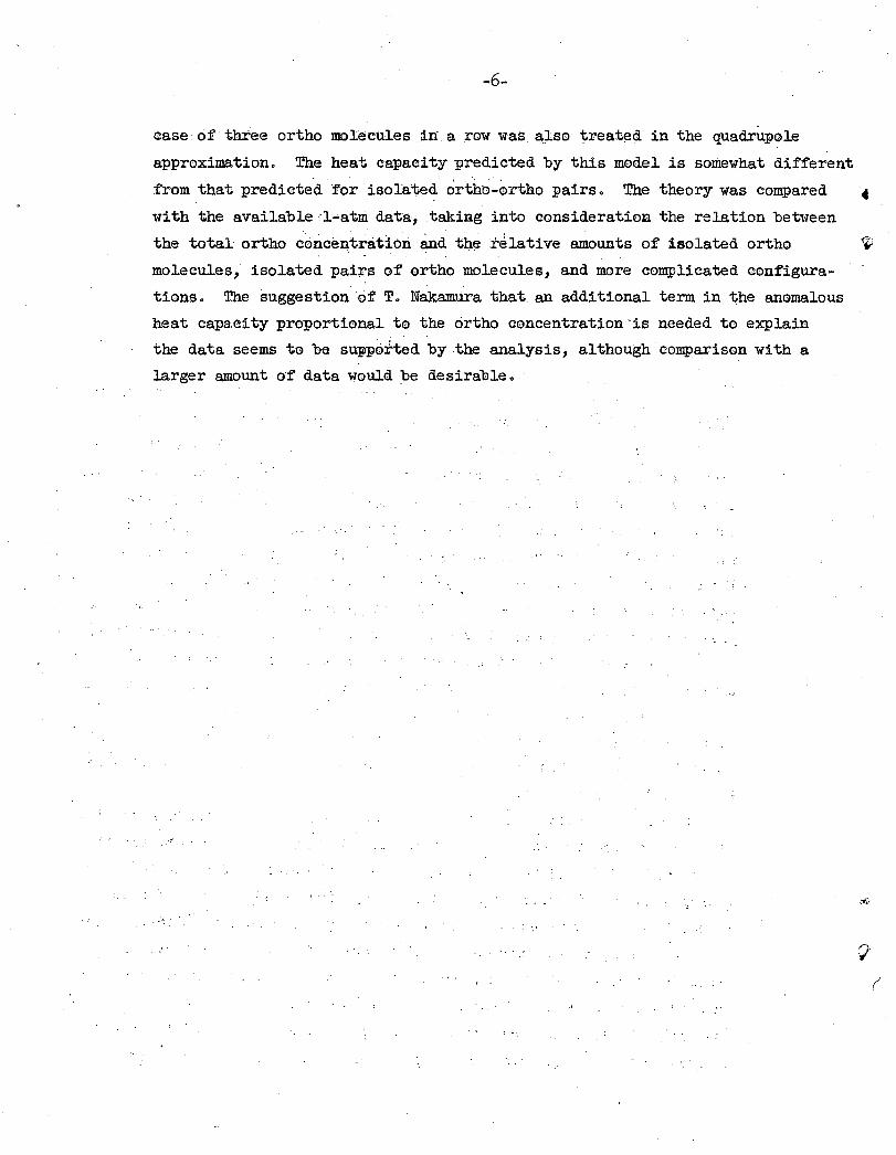
case of three ortho .mol"ecules in a row was. also treated in the quadrupole

approximation. The heat capacity predicted by this model is somewhat different

from that predicted for isolated ortho-ortho pairs. The theory was compared

with the available'l•atm data, taking into consideration the relation between

the total ortho concentration and the relative amounts of isolated ortho ~

molecules, isolated pairs of ortho molecules, and more complicated configura­

tions. The suggestion ·of T. Nakamura that an additional term in the anomalous

heat capacity proportional to the ortho concentration-is needed to explain

the data seems to be supported by the analysis, although comparison with a

larger amount of data would be desirable"

·. . . . .·:

: ·.•

(

-7-

THERMAL PROPERTIES OF SOLID HYDROGEN UNDER PRESSURE

I. INTRODUCTION

The simplest system exhibiting molecular ~otation in the solid state is

hydrogen. Examples of more ·complicated molecules that are known to rotate

in the solid phase are fairly numero_us. Metha.rie and ammonium ions in some

salts are the most commonly known. Although solid hydrogen would appear

to be the simplest of this series, the number df unsolved problems and I

unanswered questions relating to it is still quite large, as will be seen

from th~ following discussion.

As ·is well known, the idea of a proton spin, combined with the Pauli

· principle, led to the discovery of the ortho and para modifications of the

hydrogen molecule. Since the conversion of.the syimnetric nuclear state

(ortho) to the antisymmetric nuclear state (para) is forbidden in the absence

of an inhomogeneous magnetic field, the two species are not in thermal

equilibrium with each otl:Br during experiments of relatively short duration.

The significance of this fact for the present discussion is readily seen.

In liquid (20 to 14°K) and solid (below 14°K) hydrogen, the ortho molecules

are in the lowest antisymmetric rotational state (J = 1) and the para mole­

cules are in the lowest symmetric st·ate ( J = 0 ), even though the thermal . 0

equilibrium at 20 K has only about 0.2% of the ortho species. For this

reason, it is possible to study the rotating species in the solid state.

The high temperature or statistical equilibrium is three-fourths ortho

hydrogen, and until very recently, this was the highest fraction of ortho

hydrogen available for experiments. The situation in the deuterium molecule

is somewhat different because the nuclei have different spin and statistics.

* The highest fraction of the rotating species (para) obtainable thermally is

only one-third in this case.

An over-all discussion of the nature of solid hydrogen and deuterium

must cover crystal structure, lattice vibrations, interactions between

neighboring ortho molecules, the cooperative phenomenon at about L5°K,

* By convention, the mos.t abundant high•teJ,DPerature species is. ortho, and

the other para.

-8-

the kinetics of the ortho-para conversion in the solid phase, the nature of

the nuclear magnetic resonance (NMR) spectra, and the effect of pressure on

lattice and rotational -prb.perties.

Keesom, DeSmedt9 and Mooy determined the structure of pure para hydrogen

at liquid-helium temperature in 1930,1 and ~oncluded that the structure was

hexagonal close-packed with a = 3 .75A and c/a = 1..633. Recent work by Kogan,

Lazarev, and Bulatova on the crystal structure of solid deuterium indicated

that it is tetragonal with c/a = 0.94 and a= 5.4A. 2 These values gave a

density of 0.18 g/cm3, within lo% of the experimental value. These authors

reexamined the analysis of Keesom et al. and decided that their data could

also have been interpreted in terms of a tetragonal lattice. Evidence was

found for double refraction in:.both hydrogen and deuterium.' In a later

communication on the phase diagram of the hydrogen-deuterium system,3 the

same authors discovered a solid-phase separation below 16.4°K. An X-ray

study of the mixtures at 4°K revealed that the hydrogen-rich and deuterium­

rich phases had different crystal structures that differed only slightly

from those of pure hydrogen and deuterium. In this paper, the authors 'did

not think it possible to accurately .determine the structure of either

hydrogen or deuterium. They conclude only that the structures of hydrogen

and deuterium are different and the Leiden assignment was incorrect. No

mention of the ortho-para composition was given,. in the Russian work,?,3

leading one to suspect that high-temperature equilibr¢um mixtures were used.

Since this would be 75% rotating hydrogen and 33% rotating deuterium in the

Russian work, and no rotating hydrogen in the Leiden work9 the possibility

that the structure is 13. function of ortho concentration may not have been

ruled put.

The first measurements of the heat capacity of solid hydrogen in the

liquid-helium temperature range were published in 1931 by Mendelssohn, 4 '

Ruhemann, and Simon. Mixtures containing 75, 50, and o% ortho hydrogen

were studied over the temperature range 2 to 11°K. However, the data below

5°K were affected by the adsorption of the helium exchange gas. The data

on para hydrogen were fitted to a T3 law corresponding ~o a Debye G of 91°K.

The samples containing o~tho hydrogen gave an additional contribution to the

heat capacity below 12°K which was greater for 75% than for 5o%: ortho hydrogen.

Since a phase separation or a phase separation combined with a rotational

anomaly proportional to the orhto concentration would predict the reverse,

these possibiiities seem to have been ruled out. ~is point is of interest

-9-

in connection with diffusion in the,solid, wh:ich.is dd.scussed below.

In 1930 Pauling published a theoretical paper dealing with the rota­

tional motion of molecules in crystals.5. The limiting cases of oscillation

and rotation were considered, and it was shown that in solid hydrogen just

below the melting point, a state of almost free rotation existe.d for the

ortho molecules. At lower tempe~atures, it was postulated that the rota­

tion would be frozen out. Pauling proposed that "the solid solution becomes

unstable relative to phases of definite composition", or that both the triple

degeneracy of the J = 1 ortho state and the entropy of mixing of·the ortho

and para hydrogen would be lost in the freezing-out process in order to explain

the observed zero-point entropy of R ln 3 per mole of ortho hydrogen. . In the

same year, Simon6

pointed out that the zero-point entropy of n-H2 (for values

of kT large compared to nuclear-interaction energies) is R ln 4 (entropy of

mixing ·of ortho and para plus ortho nuclear degeneracy) and that only R ln 3

per mole of ortho hydrogen is involved in the rotational anomaly.

In an attempt to explain the vapor-pressure difference or ortho and

.para hydrogen, Schaefer7 found that the least complicated angular potential

pertaining to a hydrogen molecule in a hexagonal close-packed crystal was

the spherical harmonic, Y4. A s~cond-order perturbation calculation indicated

that a 1000-cal potential barrier was necessary to explain the data on this

basis. The use of a potential based on the spherical harmonic, Y~, gave the

more reasonable value of 28.2 cal, corresponding to an energy difference

between ortho and para hydrogen of 7.5 cal/mole at 0°K in the solid state.

The above comparison was made by using a Schottky-type anomaly for the heat

capacity. In order to obtain a good fit, it was necessary to assume that the

potential increased slightly as the temperature decreased.

In 1954, Hill and Ricketson measured the heat capacity of solid hydrogen

in the range l.l5°K to. the triple point (14°K) and discovered a A.-type anomaly

60 8 at l. K in normal hydrogen. The temperature of the A. anomaly was found to

decrease with decreasing ortho hydrogen concentration, and no.anomaly was

found at 56% ortho hydrogen above l.l5°K. The total anomalous entropy was

found to be within a few tenths of an entropy unit of R ln 3· A year later,

the measurements were extended to 0.2°K~9 ·The lowest concentration at which

the anomaly occurred was about 63% at 'a temperature of l.l °K.

In a theoretical paper in 1955, Tomita.attributed the crystal-field

splitting in ortho hydrogen to electric-quadrupole interaction between ad­

jacent ortho molecules and treated the heat-capacity anomaly as a cooperative

-10-

. 10 phenomenon. A treatment corresponding to the.Bragg-W:illiams.approximation

was given .first. •This appro~ch was unsatisfactory because (a) it did not

predict an ortho concentration below which the anomaly would be absent, and f

(b) it did not predict a residual heat capacity above the anomaly. A cal-

culation corresponding to the Bethe-Peieris approximation was then carried 0

out. The effect. of ortho c·oncentration on the critical temperature was

predicted fairly well by this theory, but the lower limit in ortho concentra­

tion for which a critical temperature can exist was predicted to be only

16.7%. No comparison was made with.the residual heat capac~ty above the

anomaly.

Translational effects in the lattice of solid hydrogen, aside from

their intrinsic interest, are also of importance in the considerations of the

splitting of the rotational degeneracy and in the ortho-para conversion

kinetics. The first heat-capacity measurements on para hydrogen4 and normal

deuterium11 (above the region of the anomaly) gave Debye Q valu~s of 91°K

and 89°K, -respectively. These values were obtained by fitting t~e Debye

theory to C data. The direct calorimetric determination of C for hydrogen p . . . v . and deuterium was then carried_ out for the 1-atm molar volumes at 11.20 and

ll.60°K, respectively. 12 The data were fitted by Debye Q's of 105° and 97°K, . 0

respectively. Megaw corrected the above values for the volume at 0 K and

found QD = lll and lo8°K for hydrogen and deuterium, respectively.13 Recent 8 14 . 40 .

more-accurate data on hydrogen and deuteripm below l K indicate that

C. does not follow a ~ law in this region, and that the original data of p 4 . .· .

Mendelssohn, Ruhemann, and Simon were appreciably too large. .

The zero-point energy of the lattice predicted by the Debye theory is

given by E0 = (9/8 )(NkQD). Using QD = lll and lo8°K, one obtains ~249 and 242

cal/mole, respectively.. Comparison with the potential energy of the crystal

(predicted from gas in[perfections) at the known molar volume indicates that

the Debye·theory gives too large zero-point energies. Since the hydrogen

molecules in. the solid d_o not .move in .a harmonic po·tential well,_ this devia- ~

tion is not surprising. By combining the expression for the zero-point energy

of a particle in a spherical box with that for a quantized mean free path,

London succeeded in-describing the properties of liquid helium near absolute

zero. l5 Hobbs appli~d the same treatment to solid hydrogen and deuterium,

obtaining zero-point energies of 162 and 123 cal/mole, which, when combined

te l1 t t . •th . t 16 ·with the po ntial ene:r;gie s, gaye exce . en agreemen . w~ ex:perJ.men •

~

..._,

-11-

The first study of the kinetics of the ortho-para conversion in the solid

and liquid phases was made by Cremer and Polanyi, in 1933} 7 · The conversion

velocity was found to be independent of temperature in both the liquid (14 to

20°K) and solid (4 to 12°K)regions. The reaction was second order in the

ortho concentration, and the rate constants were 17.5 X·l0-5 and 11.2 x 10-5

per hour per percentage unit of ortho concentration in the solid and liquid

phases, respectively. 1~ The higher rate in the solid phase reflects the

higher density of the solid. It was observed that the rate of. reaction in the

solid phase decreased as the ortho concentration became smaller, and approached

a limiting concentration. A later study was made by Cremer to investigate

this phenomen6n. 19 It was found that the decrease in rate did not occur in

the liquid phase or in the solid phase just after being frozen (regardless of

the initial concentration of ortho). Cremer concluded that self-diffusion

was very limited in solid hydrogen and that the residual ortho molecules were

isolated from each other. EXperiments gave 19 2:. 5% as the residual ortho

concentration. Since this value is greater than would be predicted statisti­

cally, it was suggasted that some neighboring ortho molecules were in unfavorable

positions for reaction. In a third paper in the same series, Cremer made a

theoretical estimate of the course of the reaction, assuming the ortho molecules . 19

fixed. Comparison with the data allowed him to make the following estimates

of the self-diffusion coefficients in solid hydrogen:· D11.3

oK :S l.5·x lo-17; -17 -15 -15 2/

Dll.BoK = 3 ::!::. 3 x 10 ; D13 •2oK = 1 ::!::. 0.2 x 10 ; D13•6oK ~ l. 7 X 10 em 1 day. From the temperature dependence of the self•diffusion, a heat of activation

of 790 2:. 130 cal/mole was obtained.

For comparison, recent NMR work by Rollin and Watson20 and Bloom21

on the

10°K self-diffusion transition has given values of 350 and 380 2:. 20 cal/mole,

respectively, for the activation energy of self-diffusion. Smith and Squire

studied the effect of pressUre on the self-diffusion transition and obtained

350 ::!::. 50 cal/mole for the activation energy at 1 atm. 22 They estimated the

correlation time (the· average time an ortho molecule spends on a lattice site

daring the self-diffusion process) to·be 2 x 10-6 sec at 10°K and 230 atm.

Cremer's method of calculating the final ortho concentration19 is of

··interest and is sUmma.rized here. l9 The reaction mechanism is ·assumed to be

o + o = p + o, where o denotes ortho and p denotes para. The crystal structure

-12-

is assumed to be cubic close-packed, so that the twelve neighbors of any

molecule fall on six straiiht lines intersecting the molecule. For .hexagonal

close packing, zig-zag lines must be drawn. The problem is first. treated for 1 the linear case, and the final ortho concentration is calculated as a function

of the initial concentration. The three-dimensional case is treated by assumin~

that the reaction first proceeds along one direction. The resulting concen­

tration is then used as the initial concentration for reaction alon,g another

direction, until all six direction have been used. The calculation predicts

a final concentration of about 12% for an initial concentration of 75%. When

the mechanism o + o. = ,P + p was considered, lower final concentrations resulted.

·A quantum-mechanical treatment of the ortho-para conversion kinetics in

solid hydrogen has been carried out by Motizuki and Nagamiya. 23 The inter­

action between two adjacent ortho molecules leading to conversion of one of

them is taken to be the magnetic interaction between nuclear spins on adjacent

molecules and between the rotational moment of one molecule with the nuclear

spins of the other. Perturbation theory is used, and the matrix elements

are expanded in powers of the mean distance of the neighboring mo.lecilles in

the crystal. The lattice modes are assumed to be expressed by the Debye

theory, and the probability of ortho-para transition with the simultaneous

emission of phonons is calculated. In solid hydrogen, the rotational energy

is larger than the largest lattice-mode energy, so that a one-phonon emission

is not possible. Two-phonon emission is found to be the dominant process,

with a contribution from three-phonon emission. The calculation is in very

good agreement with experiment.

Motizuki carried out an analogous calculation for the ease of solid

deuterium. 24 There were several important differences between the cases

of solid hydrogen and deuterium that had to be considered. First, the spin

of the deuterium nucleus is 1 and Bose statistics are followed. In the lowest

rotational state ( J = 0), nuclear :states I = 0 and I = 2 are found. In the

first rotational state (J = 1), the nuclear state I = 1 occurs. Second, the

deuterium nucleus has an electric-quadrupole moment which interacts with the

quadrupole moment of adjacent para (J = 1) mblecules. In the case of the

para-para interaction, both the nuclear-magnetic .9.nd electric-quadrupole

effects contribute to the conversion rate, and the:·kinetics are second order

as with hydrogen. The magnetic interaction between para nuclei and ortho

nuclei with I = 2 has a concentration dependence of the type c(lOO - c),

-13-

where c is the percentage of para· deuteritllli. · The net ~ee.ction rate is

de dt =

2 . . ( . ) - k c -·k' c 100 ... c Q (l) : ., .

The calcuJ.a.tion gave the resUlt that k and·k' were ·both about·l x 10-6

per hour per percentage unit. Hence the quadratic terms approximately

cancel, and the net reaction rate is·proportional to c.

The fact ~hat the Debye Q for deuterium is almost the same as that for

hydrogen, while the rotational energy is· one-half that of hydrogen, indicates

·. that one-phonon emission is possible in the case of deute:dum~ Motizuki did

not look up the experimental valu~ of GD for deuterium ( lo8°K), but guessed

·a value of 64.4°K on the basis of the harmonic-oscillator approximation,

and so missed this point. Accurate data on the para-ortho conversion in

solid deuterium do not s·eem to have-been reported in the literature as yet.

Of the many recent NMR studies made on solid hydrogen, the work of Reif

and Purcell seems most pertinent _to the present experiments. 25 These authors

studied the change in line shape as a function of temperature below 4°K. At

4°K, a simple line of 18 kcjsec width was observed. Below 1.5°K9 the line

was flanked by two side peaks .which grew in intensity at the expense of the

central line as the temperature was lowered still further. At l~l6°K, there

was still a vestige of the central linea Upon warming to 1.35°K, the line

underwent a rather rapid change of shape which did not reverse itself when

the sample was again cooled to 1.16°K and held there for several hours. The

cause of th:i.s hysteresis could not be explained.· The -shape of the resonance

line below 1.5°K was explained in terms of a general crystal field of

spherical harmonics of second 6rder. The resUlting splitting of the three

sublevels was large· enough to quench the rotational Ilia.grtetic mement of the

ortb.O molecules. The high-frequen-cy transitions between the split rotational

levels could be neglected in the NMR so·tba.t each of the. tll:ree rotational

. sublevels gave rise to -two resonance lines •. A rough calcUlatioh .of the rate

of transition between the rotational sublevels indicated that it was greater

than the nuclear dipole-dipole splitting ·in an orthcf molecule (expressed in

kc/sec ). In this case the dipole-dipole interaction shoUld be averaged over

all of the rotational sublevels·, :with each weighted according to its Boltzmann

factor, rather than over the probability di-stribution of a single sublevel.

-14-

The authors carried out both calculations, and fotmt;i that both .g~ve essentially

the same line shape. The remnant central line at low te~eratures was explained

by the presence of some ortho molecules with a small number of ortho~molecule ~

neighbors. The line shape also indicated that the sublevels of a large number

of ortho molecules were split by amounts larger than E/k = 4°K. ~

Studies of pressure effects in solid hydrogen have become of interest

in recent years, although some earlier work is important. ~-legaw m~asured . ' 2

the compressibility of' solid hydrogen and deuterium f'rom l to 10.0 kg/em at

4.fPK.13 The molar volumes of hydrogen and deuterium at 1 atm were found

to be 22.65 .:_ 0.1 and 19.56 .:_ 0.1 om3; respectively. The volumes at 4°K were

assumed to be the same as those at 0°K. The compressibilities were 6.8 + ~ -4 4 -4 2 11• I 2 -4 -1.5 x 10 · and .5 ~ 2 x 10 em fAg at 1 kg em and about 3.2 x 10 and

-4 21!.~ ,J 2 2.1 x 10 em /A5 at 100 kg1 cm , respectively. Simon obtained for the pressure

and compressibility due to zero-point energy predicted by Debye theory 26

Po = g R Y·~ (2)

and

t3o v

= * RQ r(r + 1) , (3)

where Q is the Debye temperature, v is the molar volume, and r = d log Qjd log v

is GrUeneisen•s constant. These results were applied to the data, and it was

shown that the experimental compressibili ties were predicted very well by the '

above eXpression.

Stewart27, 28 measure'd the compressibility of solid hydrogen and deuterium

at 4.2°Kup to 20,000 kg/cm2• 27, 28 The molar volume and compressibility ·. 13

of' hydrogen (based on Megaw's 1-atm value ) were found to be greater up to

the highest pressures, indicating to Stewart th:at the zero-point energies

.. were still of importance.

these measurements;

No phase changes seem to have been discovered by

· Tre ef'f'e~t of' pressure on the rotational levels of hydrogen molecules

in the solid has been considered by London.29 A summary of the effect of a

hindering potential on tl::e rotational states of a diatomic molecule in a

crystal was given earlier by Pitzer.3° With a smail potential barrier, the

rotational states are the same as in the gas phase, while with a higp·barrier,

the rotation becomes a torsional oscillation. The gas-phase rotational states

-15-

J = 0 and J = 1, M = 0 converge and become degenerate for a homonuclear

diatomic molecule when the potential barrier to.rotation becomes infinite •

. Since solid hydrogen has a large compressibility, London proposed that it

might: be possible to increase the rotational barrier sufficiently to bring

the above-mentioned states very close in energy e He pointed out that if

one started with para hydrogen and compressed the solid to the point where

the: ·para and m = 0 ortho levels were essentially degenerate, a- large increase

in entropy (R l.n4) would be obtained if' the para hydrogen could convert to

the statistical mixtUre of' nuclear states. The above mechanism would

constitute a powerful, but hardly practical, cooling mechanism in the

vicinity of' 1 °K.

London interpreted the large compressibility of solid hydrogen by

assuming that the initial work of compression was used to reduce space for

the molecules by confining their rotational motion to a smaller angle. Since

the crystal potent,ial barrier may be thought of' as being erected at the node

of' the J = 1, m = 0 wave function, most of' the compression energy should go

into increasing the energy of the para molecules. On this basis, London

made a rough estimate of' the pressure required to raise the J = 0 level to

the J = 1, m = 0 level by assuming that all of' the compression energy went

into raising the J = 0 le~el. Since the J = l level would also be raised

somewhat in compression, he doubled his estimate and obtained a pressure of

the order of' magnitude of' 10,000 kg/cm2 • An objection might be rai~ed to

London's calculation on the grounds that between 1 and 5000 kg/cm27 most

of the compression energy probably goes into increasing the zero-point

energy of' the crystal:,_rather than changing the relative energies of the

ortho and para species. Above,5000 kgjcm2, however, 'one might expect steric

hindrance to become important, so that the pressure estimate of' 10,000

kgjcm2 may still be reasonable. In a theoretical calculation of' the .non­

spherical potential field between two hydrogen molecules, deBoer used the

Heitler-London-Wang wave functions for the hydrogen molecules, and calculated

the inter-molecular potential curve for various relative .. ori~ntations of the

molecules.31 Consideration of these results also indicates that the hindering . '

potential becomes appreciable _in t~e pressure range between 5000 and 10,000 atm.

The effect of pressure on the NMR down to 1.2°K was studied by Smith and

Squiree 22 They did not detect any change in line shape or Shift in the 1.5°K

rotational transition temperature at pressures up to 337 atm. McCormick and

\ -16-

Fairbank, in an attempt to obtain some data relating to London's theory, 32 studied the nuclear resonance to a pressure of· 5000 atm. .. The. ;shape and

amplitude of the lir.e at 4.2°K remained constant to this pressur;e, but the

tra~si tion temperature 1-1as observed to increase. The ortho-para .conversion

rate remained small to 5000 atm, as indicated by the rate of change of the ~.

amplitude of the resonance line •.

The present experiment~ were undertaken with the hope of studying the

properties of solid hydrogen in the interesting region above 5000 atm. The

two methods of measurement considered for this study were NMR and heat

capacity. Results from these methods would give the same information in

some ways (such as the temperature of the anomaly as a function of pressure)

and complimentary information in others. Since work on the nuclear resonance 22 '

seemed well advanced in other laboratories· and since the heat-capacity data

woUld be extremely'interesting.in any case;. it was decided to attempt the

thermal measL~ements.

The plan of the experiments was to measure the heat capacity in the

region 1.1 to 20°K. as a function of pressure and ortho concentration. The I

change in the L~teraction between neighboring molecules with pressure was the

phenomenon to be studied. In more specific terms, the effect of pressure on

the splitting of the rotational sublevels, the shape of the anomalous heat

capacity, and·the lattice heat capacity was of interest •. The same·apparatus

could be used to study the rate of conversion of ortho to para l:J.ydrogen as

a function of density.

The f'irst part of this report is essentially a description of' the apparatus

necessary to carry out the above experiments. The basic problem was to compress

a sample of hydrogen into a ceJ_l in which .its heat capacity could be measured.

The solution of the problem involved the construction of special apparatus

and the development of the techniques ne,cessary to obtain tb,e data.

'. \ ••

-17-

II. CALORIMETER

General Description

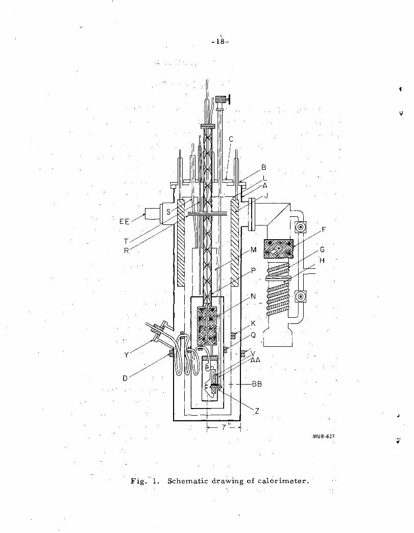
The general layout and main features of the ca;Lorimeter are shown in

the schematic diagram in Fig. 1. The outer vacuum can, A, was aluminum,

and the top flanges, B and c, were stainless steel. There was also a flange,

D, near the bottdm for access to the cell. The pumping system was connected

to the main vacuum can through the pipe, E, and consisted of a Temescal 4-in.

gate valve,. F, a water-cooled baffle, G, a Consolidated Electrodynamics MCF-

300 Qil-diffusion pump, H, and a KC-6 Kinney forepump. A High Voltage

Engineering ion gauge was attached at EE. The liquid nitrogen reservoir, J,

was suspended i'rom the flange, B; by six tubes. A copper radiation shield

was attache.d. to the bottom of the reservoir and was detachable at K. A

copper shield arrangement, L, was connected to the top of the reservoir to

keep room-temperature radiation out of the'top. Four concentric cylindrical

dimpled stainless steel sheets. were loosely attached to the inside of the

reservoir above K t0 act as radiation shields. Ten sheets of a similar

nature were placed below K and across the bottom of the shield.. The vacuum

can, pumping system, and liquid-nitrogen reservoir were adapted f"rom a standard

accelerator target design in use at the Lawrence Radiation Laboratory. The

liquid-nitrogen bath was arranged so that it could be pumped down in order to

reduce :the heat leak. to the inner parts of the apparatus for certain experiments.

Two baths were necessary for the iiquid hydrogen or helium. The purpose

of the outer bath, M; was to absprb the. heat leak. f"rom higher temperature, so

that the inner bath, N, could be pumped to the vicinity of 1°K with a pump of

moderate capacity. Although the outer bath made the calorimeter a good bit

more complicated, the shortness of the apparatus and the unavailability of

high pumping .speed made it a necessity. · The outer bath surrounded the pumping

tube of the inner bath, P, and had a copper radiation shield attached to the

bottom of it which was detachable at Q. Additional protection for the oute~

bath was provided by a pile of four disc-s:p.a.ped dimpled stainless steel discs,

R, loosely connected to the pumping tube; P, at a point about half-way to the

liquid-nitrogen shield. The pumping tube for the outer bath was located at S;

and was connected to a KS-l3 Kinney pump. The transfer tube, T, was permanently

fixed in the calorimeter because of the low ceiling. The other part of the

' -18-

c

EE

T

y

D

Fig. -1. Schematic drawing of calorimeter.

F

G H

MUB-627

'

., .,

v

-19-

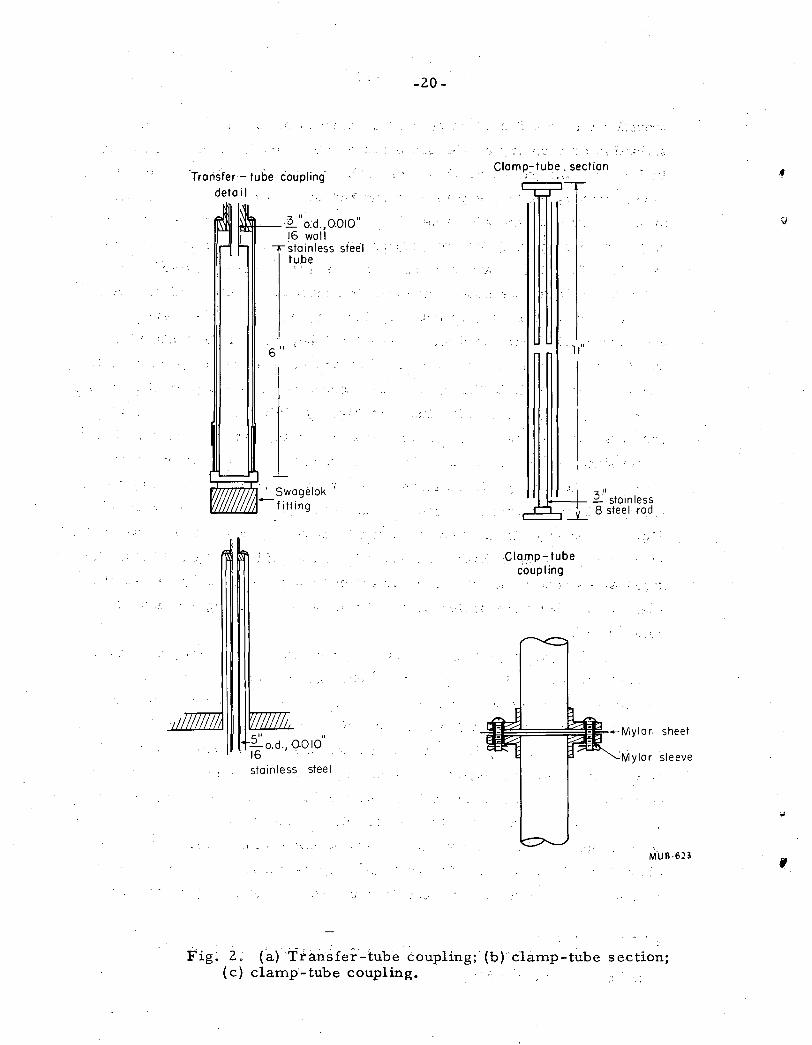
transfer tube could be dif;connected at the top of the calorimeter. The

mechanism of coupling of the two parts of the transfer tube is illustrated

in Fig •. 2. The jacket of the outer-bath transfer tube was part of the main

vacuum system, while a separate vacuum had to be pro~ided for the jacket

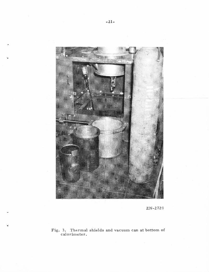
of the inner-bath transfer tube, U. Two·well..;baffled holes were put in the

copper shield be~ow Q for the purpose of evacuating the inner part (see

Fig. 3). The baffles and the inside of the shield were painted black in

* order to minimize the amount of radiation reflecting in toward the cell. ~ ~.

The inner bath was supported by its pumping tube. The transfer tube

was permanentiy positioned in the pumping tube, and a spiral stainless

steel radiation shield, painted black at the bottom; was suspended in the

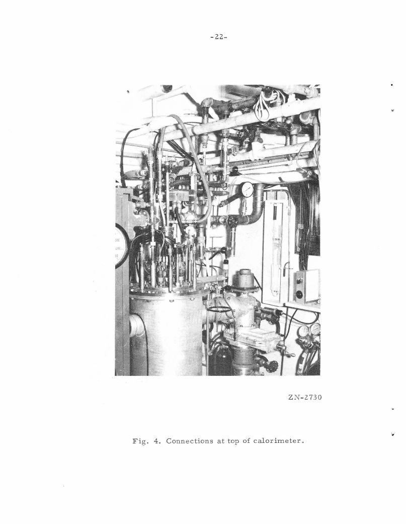
pumping tube. A KD-30 Kinney pump was connected to the top of the pumping

tube through a 3.;.in. copper line (see Fig. 4). The isothermal shield

consisted of a block of copper and lead at the top and of a copper shield

surrounding the cell, W. The shield was mechanically co·nnected to the

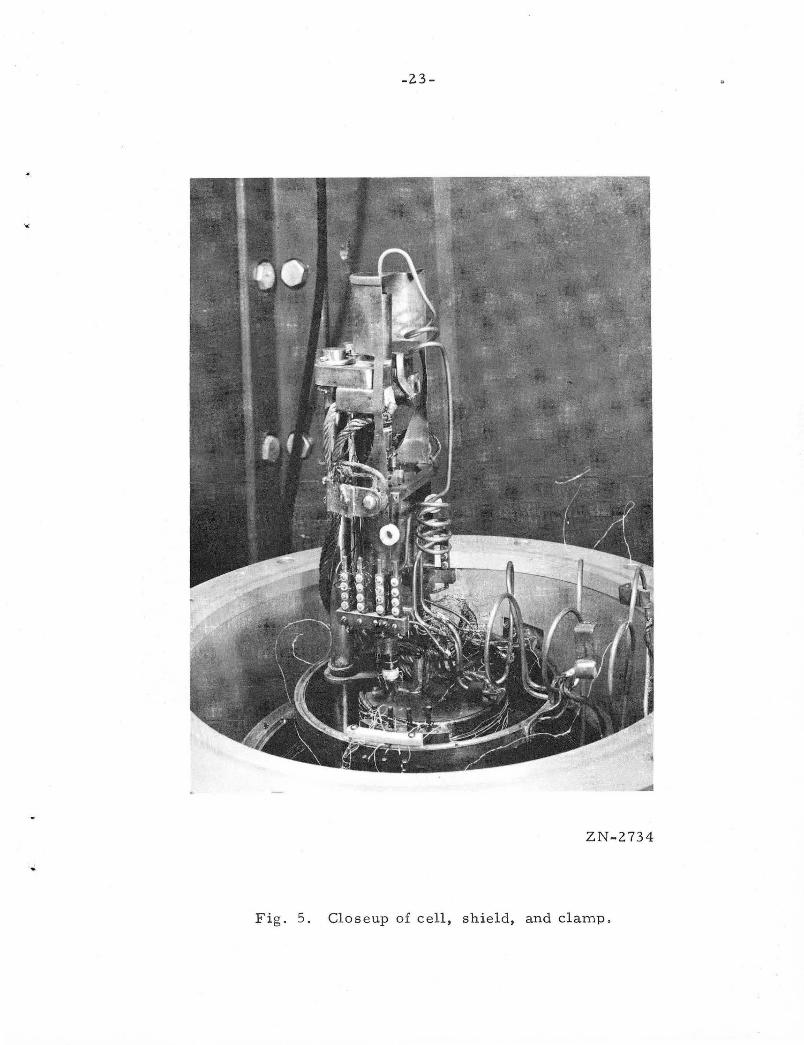
inner-bath bottom by two stainless steel rods. The cell was supported in

the shield by the stainless steel p:ressure capillaries, X, as shown in

Fig. 5· The capillaries were in thermal contact with the isothermal shield,

inner bath, and outer bath, but not with the liquid-nitrogen shield. The

capillaries passed out of the calorimeter to the pressure system at the

flange, Y. They were sealed to the flange with Armstrong Products Co.

epoxy resin.

A double-jaw-type thermal clamp, z, was used for cooling the cell.

It contacted _the cell on two flat 1/4-in.-thick copper faces. It was

connected thermally to the inner bath '\4i th a flexib.le copper connection 2 '

·of about. L em cross section. The clamp was operated mechanically by two

stainless steel tu,bes; M, passing out the top of the calorimeter, and

externally c·onnected together by means of gears. An au.:x:iliary clamp was

connected to the tubes for cooling the shield. A worm-gear arrangement

was used to open and close the clamp. Rotary vacuum seals enabled the clamp

to be opened and closed without disturbing the vacuum. The section of the

clamp tubes between the outer bath and liquid-nitrogen bath was made from

several different diameter tubes to inc:rease the path length ahd reduce the

* Suggested by Professor N. E. Phillips, Department of Chemistry, University

of California, Berkeley.

. ; .

Transfer -tube coupling·

detail .· .. ;

3 II II

ll'frlllf-'-'--·~ o.d.,O.OIO 16 wall sto in less steel tube

Swogelok .....,.LJ....I...j.......,..- fitting

511 II

-o.d., 0.010 16 • •'

stainless steel

I '

-20-

Clomp:- tube. section . ;'· .. '

3'; . t---f-- stainless

8 steel- rod. _,__

Clomp-tube coupling

·..::·

~~3i===~~ff---Mylor. sheet

'Mylar sleeve

MUB-623

Fig: 2. (a) T:i-ansfer-tuhe coupling; (b) clamp-tube section; (c) clamp-tube coupling.

,f

,

-21-

ZN-272 9

Fig . 3 . The rmal shields and vacuum can at bottom of calorimeter.

-22-

ZN-2730

Fig . 4. Connections at top of calorimeter .

-23-

ZN-2734

Fig. 5 . Closeup of cell, shield, and clamp .

-24-

ZN-2731

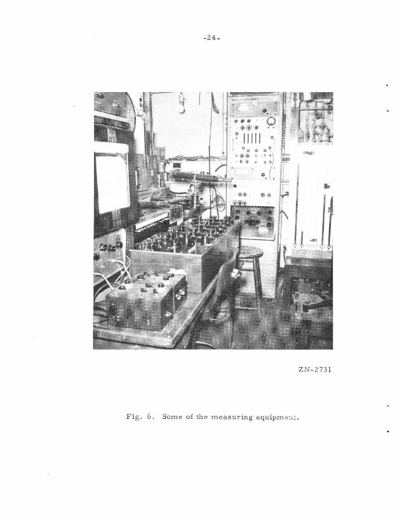
Fig. 6 0 Some of the measuring equipm er.~,

~\

·-

-25-

heat leak (see Fig. '2}. An extension 'above the main flange was also made

for this purpose. The sections of the clamp tubes were insulated from each

other by thin mylar sheets to reduce the heat leak further when the jaws

were open.

A vapor-pressure bulb, BB, was soldered to the top of each jaw so that

it would be in good thermal contact with the cell when the clamp was closed.

Each bulb was made from a' single piece of 1/16-in. copper hard-soldered into

a rectangular shape having a volume of about 4 ·cm3. A lj4-in. stainless

steel tube was hard-solder~d into the top surface for adapting to the smaller

stainless-steel tubing. The bulbs were soft-soldered directly to the copper

faces of the main clamps. Since the vapor pressure bulbs moved with the jaws,

a flexible connection was required between the bulbs and the inner bath. For

this purpose, 1/16-in. stainless steel tubing was used. It was connected to

1/8-in. tubing at the inner bath. and then run out the top of the calorimeter.

It was essential for the 'lra.por-pressure tubes leading to the bulbs to slope

downward at every point within the calorimeter.

The electrical leads were brol!lght into the calorimeter through five

3/4-in. Lawrence Radiation Laboratory fittings in the top flange, .c.. The

wires were cast. into epon plugs in the shape of the fittings. Thermal

/ contact of the wires at the liquid-nitrogen temperature was achieved by

wrapping them around a copper tube at the top of the liquid-nitrogen shield

and attaching them with G.E. 7031 cement. Contact at the two inner baths

was made by wrapping the wires around the baths twice and gluing them. A

lug post was provided on the isothermal shield for terminating· the current

and potential leads from the top of the calorimeter and for connecting

the leads from the cell.

There were several ·general reasons for designing the calorimeter in

the above fashion. By making the vacuum can and shields removable at the

cell level, it was possible to open up the calorimeter to the cell very

rapidly without disturbing any of the· electrical, thermal, or pressure

connections. · In addition, it was possible to remove the cell and pressure

capillaries without touching the thermal apparatus, and, conversely, to

hoist out the thermal parts without disconnecting the cell from the pressure

system.

Properties and Operation qf the Calorimeter Baths - . . -.- -- -...,.--~-- ~_,;...;-

Ligaid-Nitrogen Reservoir

The capacity of the reservoir was about 13 liters. A Styrofoam-insulated

tube was run from a 50-liter dewar to one of the i~let tubes, and the nitrogen ,.

* level in tbe reservoir was regulated with an automatic device. The level was

kept near the top. and did not vary more than an. inch during runs. For the

initial cooldown, it was found that a 5P-liter dewar was adequate for bringing

the reservoir to liquid-nitrogen, temperatureand for keeping it full several

hours. After the apparatus was fully cooled to liquid-nitrogen temperature,

one 50-liter dewar was .required every 2~ h;r, and the. automatic bath filler

transferred regularly at about 1-hr intervals. For the initial cooldown, the

two inner baths were also filled with liquid nitrogen. It tqok abput 3 hr for

the thermocouples on the copper parts to indicate liquid-nitrogen temperature,

but since there were several .long lengths of stainless steel tubing with a

considerable heat capacity, the apparatus .. took at least 8 hr to cool completely

to liquid-nitrogen temperature. The initial cooldown was usually carried out

over· night. The reservoir ·was: also connected to a vacuum manifold so that its

pressure could be reduced to the triple point (63.2°K) or lower in order to

reduce the heat leak,to. the outer liquid-helium bath.

Outer Liguid-Helium Bath

A rough estimate of the heat leak to the outer liquid-helium bath for

the nitrogen reservoir at 77°K is given in Table I. In.this estimate, we

assume that all radiation hitting ·the outer bath is absorbed. If the liquid­

nitrogen reservoir is pumped down to 63.2°K, the heat leak. is reduced by· 3o%·

For comparison, the heat of vaporization of liquid ~ydrogen is 32,400 joules

per liter, arid of liquid helium is 2750 joules per. ]..iter. With the nitrogen

reservoir at 77°K, liquid helium should last about 1 hr per liter. and liquid

hydrogen about 13 hr per liter. The capacity of the bath ~s 2.7 .liters.

In practice the bath was ;uslia.lly filled with 'liquid hydrogen eve.ry 12 hr

* Constructed by Jack Harvey, Maintenance Machinist Group, Lawrence

Radiation Laboratory.

.l·<r

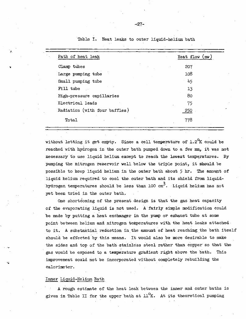
Table I. Heat leaks to outer liquid-helium bath

Path of heat leak

Clamp tubes

Large pumping tube

Small pumping tube

Fill tube

High-pressure capillaries

Electrical leads

Radiation ('with four baffles)

Total

Heat flow (mw)

207 108

45

13 80

75 250

778

without letting it get empty. Since a cell temperature of 1. 2°K could be

reached with hydrogen in the outer bath pumped down to a few mm, it was not

necessary to use liquid helium except to reach the lowest tempe:ratures. By

pumping the nitrogen reservoir well below the triple point, it should be

possible to keep liquid helium in the outer bath about 5 hr. The amo~t of

liquid helium required to cool the outer bath and its shield from liquid­

hydrogen temperatures should be less than 100 cm3. Liquid helium has not

yet been tried in the outer bath.

One shortdoming of the present design is that the gas heat capacity

of the evaporating liquid is not used. ·A fairly simple modification could

be made by putting a heat exchanger in the pump or exhaust tube at some

point between helium and nitrogen temperatures with the heat leaks attached

to it. A substantial reduction in the amount of heat reaching the bath itself

should be effected by this means. It would also be more desirable to make

the sides and top of the bath stainless steel rather than copper so that· the

gas would be exposed to a temperature gradient right above the bath. This

improvement could not be incorporated without completely rebuilding the

calorimeter.

Inner Liquid-Helium Bath

A rough estimate of the heat leak between the inner and outer baths is

given in Table II for the upper bath at 11°K. At its theoretical pumping

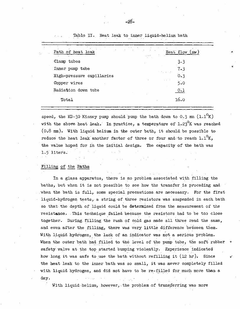
Tabl<= II. Heat leak to inner liquid':"helium bath

Heat flow (mw) Path of heat leak ~

Clamp tubes

Inner pump tube

High-pressure capillaries

Copper wires

Radiation down tube

Total

3·3

7·3

O.j

5-0

0~1

16.0

speed, the KD-30 Kinney pump should pump the bath down to 0. 3 mm ( 1.1 °K)

with the above.heat leake In practice, a temperature of 1.23°K was reached

(Oo8 mm)~ With liquid helium in the outer bath, it should be possible to

reduce the heat leak another factor of three or four and to reach l.l°K,

the value hoped for in the initial design. The capacity of the bath was

L 5 liters. ·

Filling of the Baths

In a glass apparatus, there is no problem associated with filling the

baths, but when it is not possible to see how the transfer is preceding and

when the bath is full, some special precautions are necessary. For the first

liquid-hydrogen tests, a string of three resistors was suspended in each bath

so that the depth of liquid could be determined from the measurement of the

resistance.. This technique failed beqau~e the resistors had to be too close

together. During.filling the rush of cold gas made all three read the same, - .. '

and even after t~e filling, there was very little difference betvmen them. -

With liquid hydrogen,. the lac~ of an indicator was not a serious problem.

When the outer bath had filled to the level of the p~p tube, the soft rubber +

safety valve at '!=-he t~p .star.te.d bumping violently. Experi·ence indicated . ·.. . ·' . . .

how long it was safe to use the bath without refilling it (12 hr ). Since -;;'

the heat leak to the inner bath was. so small, it was never completely filled

with liquid hydrogen, and did not have to be re-filled for much more than a

day.

With liquid -helitim, however, . the problem of trans,fer~ing was more

...

-29.:.·

serious. The safety valve did not bump when the bat~ was full, so that a

large amount of liquid could easily be blown out the vent. ,.An oil-manometer

flow gauge was connected to the yent to give an indication of the rate of

evaporation of the liquid, and a thermocouple attached to the outside of

the bath was monitored during the transfer.; Initially, the fi0w out the

vent was large because of the cooling of the transfer tube. There was

then a lull, followed by a second large flow. At first the second flow

was interpreted as indicating that the bath was full; however, it turned

out that this was just the beginning of the filling of the bath. The amount

of liquid helium lost during each transfer was about l liter or less.

Descriptiop of the Cell and Environment

Isothermal Shield

The top of the shield was a 3-in.-diam. by 5/8-in.-thick copper disc.

A cylindrical 0.022-in. copper shield 8-1/2-in. long was soft-soldered to

the bottom of the copper disc. The shield was sliced in half vertically and

held together with two copper screws thro)lgh the disc. The back half was

permanently attached to the inner bath by two stainless rods. The front half

was removable for access to the cell. Two half-circles of lead, each l-3/8-in.

diam. and 1/4-in. thick, were soldered to the underside of the copper disc on

. the removable part of the shield. About 30 em of the electrical leads were

coiled up between the inner bath and the shield and glued to a copper rod

screwed into the top of the back half of the shield with G.E. 7031 cement •

. The wires then went to soldering lugs on the sides of the shield. These

were simp+y b~ss screws insulated with Teflon washers from copper strips

soldered to the shield. Manganin wires went from the lugs through the shield

to the cell. They were wrapped around the end of the lug posts and glued

before going to the cell. It is thought that the largest thermal emf's in

the measuring circuits, occurred at the copper-to-~ganin joints. The

heater-regulator components (two 2000-ohm heaters and a 10-ohm thermometer)

were mounted on a copper rod screwed into the top of the back half of the

shield.

Cells

The cells were made from beryllium copper. The outside dimensions of the

first design were 6-l/4-in. long by 11/16-in. diam. The inside dimensions were

-30-

4-in. long and 1/~~-in. diam. The design .considerations for: the cell are

discussed in Section III and the heat capaci};ies are disc).lssed in Section

V. About 1000 ohras of Driver Harris 0.00175-in.- diam. Formvar-insulated

manganin -v1ire (92.30 ohms/ft) -v1ere bifila71ywound on the cell. It -v:as.

found, ne~es.sary tb put a layer of cigarette :f)aper under the· 1-rindings to

keep the leal~ge resistance to tl1e cell large enough. The windings were

glued to the cell with G.E. 7031 cement. Solder lugs on the cell were

provided by t-vm heavier copper loops glued to the cell. The potential leads

were No4 40 manganin; the current leads No. 30. The current leads were

48 ~ 2 ~n long. The use of short lengths of manganin was necessary to obtain

small enough. heat leak and electrical resistance. Two radio resistors were

used as thennometers. These were l/2-w Al:l.en-Bra.dley 10"" and 56~ohm types

with the covers ground off. '],'hey were glued in dead soft-copper clips which

were Shaped around them and glued to the cell. The leads on the resistors

served as solder lugs. The mapganin wires were wrapped around the cell once

and glued before going to the shield.

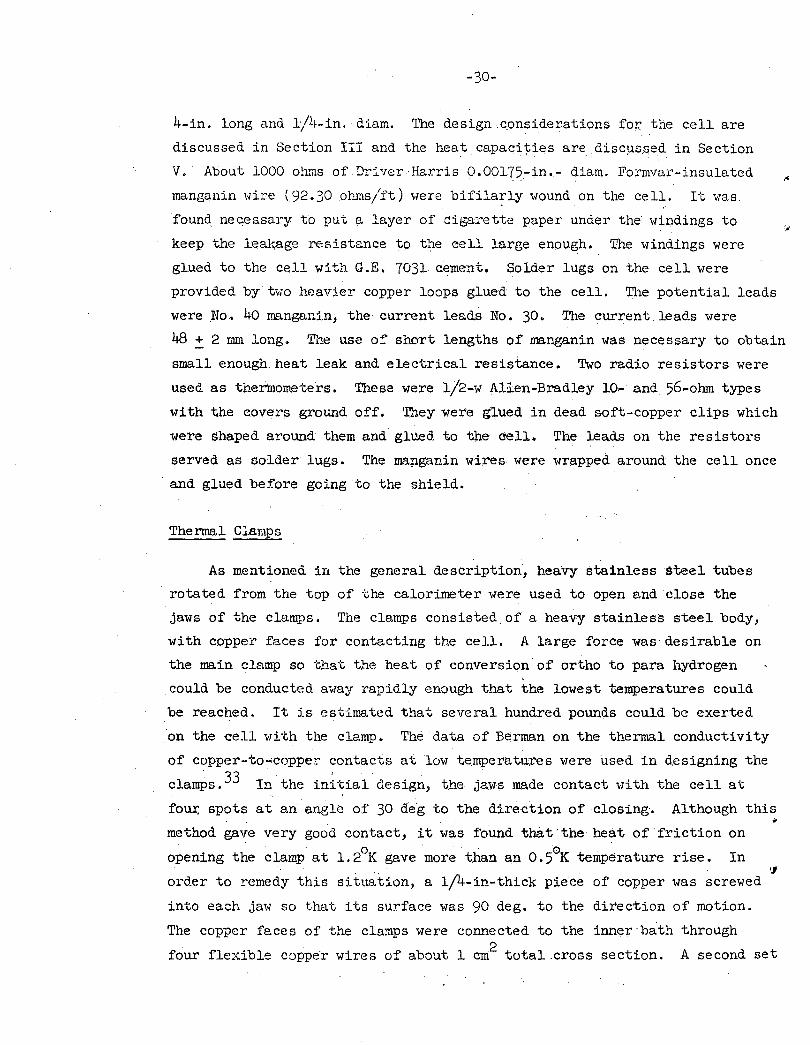
Thermal Clamps

As mentioned in the general description, heaVy- stainless steel tubes

rotated from the top of ·che calorimeter were used to open and close the

jaws of the clamps. The clamps consisted of a heavy stainless steel body,

with copper faces for contacting the cell. A large force was· desirable on

the main clamp so that, the heat of conversion· of ortho to para hydrogen

could be conducted a·.ray rapidly enough that the lowest temperatures could

be reached. It j_s estimated that several hundred pounds could be exerted

on the cell >-rith the clamp. The data of Berman on the thermal conductivity

of copper-to...;coppex- contacts at low temperatures v1ere used in designing the

clamps,33 In the initial design, the jaws made contact -vlith the cell at

four. spots at an engle of 30 Cfeg to the direction of closing. Although this

method gave very good contact, it was f'ound that·tne heat of friction on

opening the clamp at 1.2°K gave more than an 0.5°K temperature rise. In ~

order to remedy this situation, a 1/4-in-thick piece of copper was screwed

into each jaw so that its surface was 90 deg. to the direction of motion.

The copper faces of the cla~ps were connected to the inner·bath through

four flexible copper wires of about 1 cm2 total.cross section. A second set

f' ..

of clamps of a lighter design was attached to the tubes at a higher point to

contact the shield. These clamps made contact before the main jaws, but did

not exert as much force. About 1. 5 hr were required to cool the shield from

liquid-nitrogen to liquid-hydrogen temperature. The limiting process in this

respect, however, was the cooling of the stainless steel capillaries between

the cell and shield, which required 4 hr.

Vapor-Pressure Bulbs

The mechanical arrangement of the bulbs is given in the general descrip­

tion. The front bulb was usually used with hydrogen and the rear one with

helium. The sample used was placed in a 2-liter bulb at room temperature and

slightly less than 1 atm. and then condensed into the bulb. The manometers

were made from 20-mm. tubing, and-the mercury or oil (Octoil) levels were read

with a Gaertner cathetometer accurate to about + 0.1 mm. The copper-iron­

versus--copper thermocouple used as an auxiliary calibration thermometer and

a copper-constantan thermocouple were glued to the rear vapor-pressure bulb.

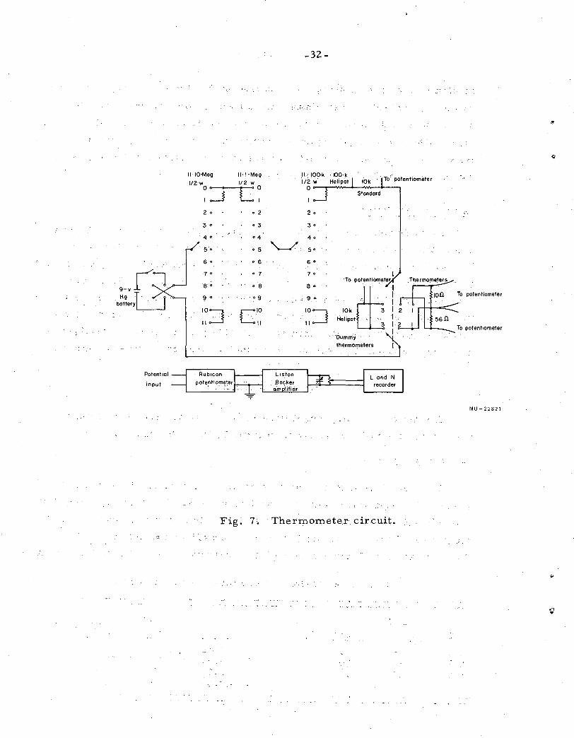
Calorime;FY Circuits

Thermometer, heater, temperature control, and thermocouple circuits

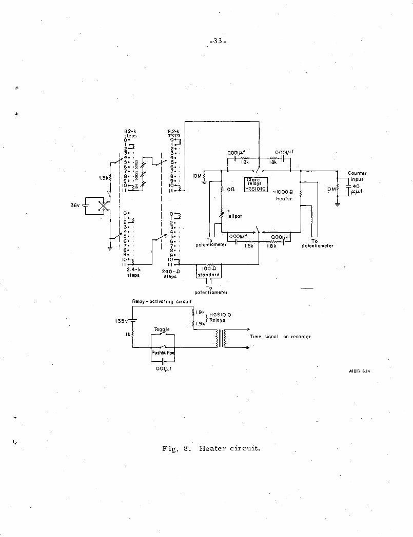
used in the calorimeter are shown in Figs. 7, 8, 9; 10, and 11.

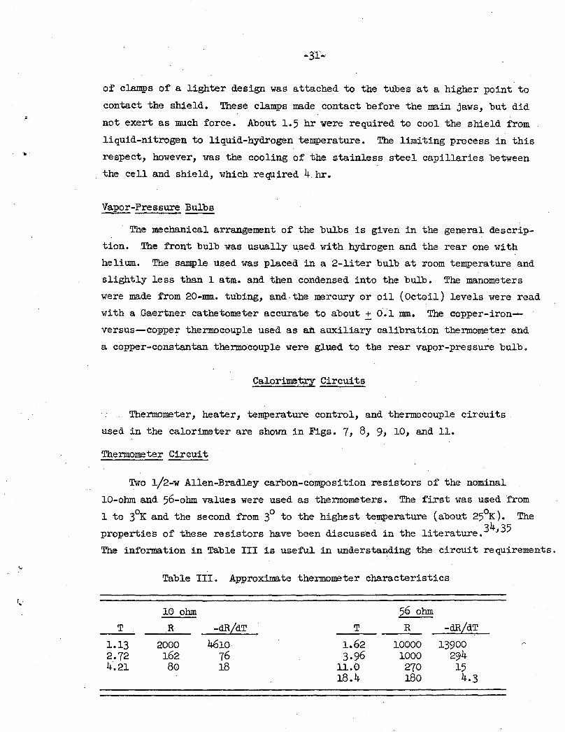
Thermometer Circuit

Two 1/2-w Allen-Bradley carbon-composition resistors of the nominal

10-ohm and 56-ohm values were used as thermometers. The first was used from

1 to 3°K and the second from 3° to the highest temperature (about 25°K). The . 4 properties of these resistors have been discussed in the literature. 3 ., 35

The information in Table III is useful in understanding the circuit requirements.

Table III. Approximate thermometer characteristics

10 ohm 56 ohm

T R -dR,LdT T R -dR,LdT

1.13 2000 4610 1.62 10000 13900 2.72 162 76 3·96 1000 294 4.21 80 18 11.0 270 15

18.4 180 4.3

9-vl:-1 Hg LJ battery

Potential

input

11·10-Meg 11·1-Meg

l/2·w 1/2 w

~:J c~ 2 0 0 2

3 0 0 3

'. ' 4• •4

. s·o' 0 5

6 0 0 6

7 0 0 7

a·· •. 8

9 0 . 0 9 :~:J C~~~

Fig; 7.

-32-

2 0

3 0

4o

'--/. 5•

6 0

7 0

8 0

9 .. o:

IO:J II

potentiometer

thermor:neters

Land N recorder

Thermornete.r. circuit.

To potentiometer

To potentiometer

MU-22821

j'i.

82-k steps o• ~~

I 3• ,

0~::\i 6. •iil 7• ''ii

1.3k ~= :Sl

I I I

10 ~ II -

steps

8.2-k steps

?:J 2• ' 3• ' 4· 5· 6· 7· 8. ' 9•

10 II

-33-

To potentiometer

Relay- activating circuit

135v 1.9 k HGS 1010

} Relays 1.9k

Fig, 8. Heater circuit.

10M

To potentiometer

input

40 JJ-J-Lf

MUB·624

[ lL.----0-e-te-c-to_r__.sensitivity

1.5-v

dry cell

-34-

200Sl

IOOSl l%,1/2w

100 .n 1%,1/2w

Low

1/)

0 Q.

4i :r

r---+--'M.-----'

5-11 potentiometer

MU-22822

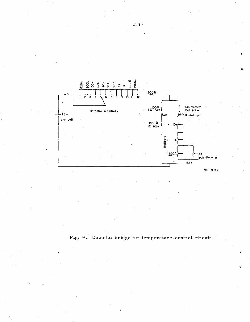
Fig. 9. Detector bridge for temperature-control circuit, ·

I· ..

-35-

..---~----~-~----~--r----~------+-•300.v

3.9k,2w

Full-scale adjustment

33k

lw IOk

3.9k,2w

5.6k, 2w

~-----+---~---------------~30.0v MU-22823

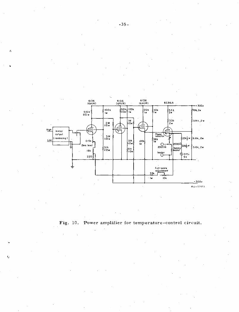
Fig. 10. Power amplifier for temperature-control circuit.

-300v

l-J ~ 15k 2w IOk 2.w

' '

-36-

' '\ ., '\ I 3

2_ok L; . :Microphone

dummy .. Connector heater -=· · to 2-k heater

· on block

MU-22826

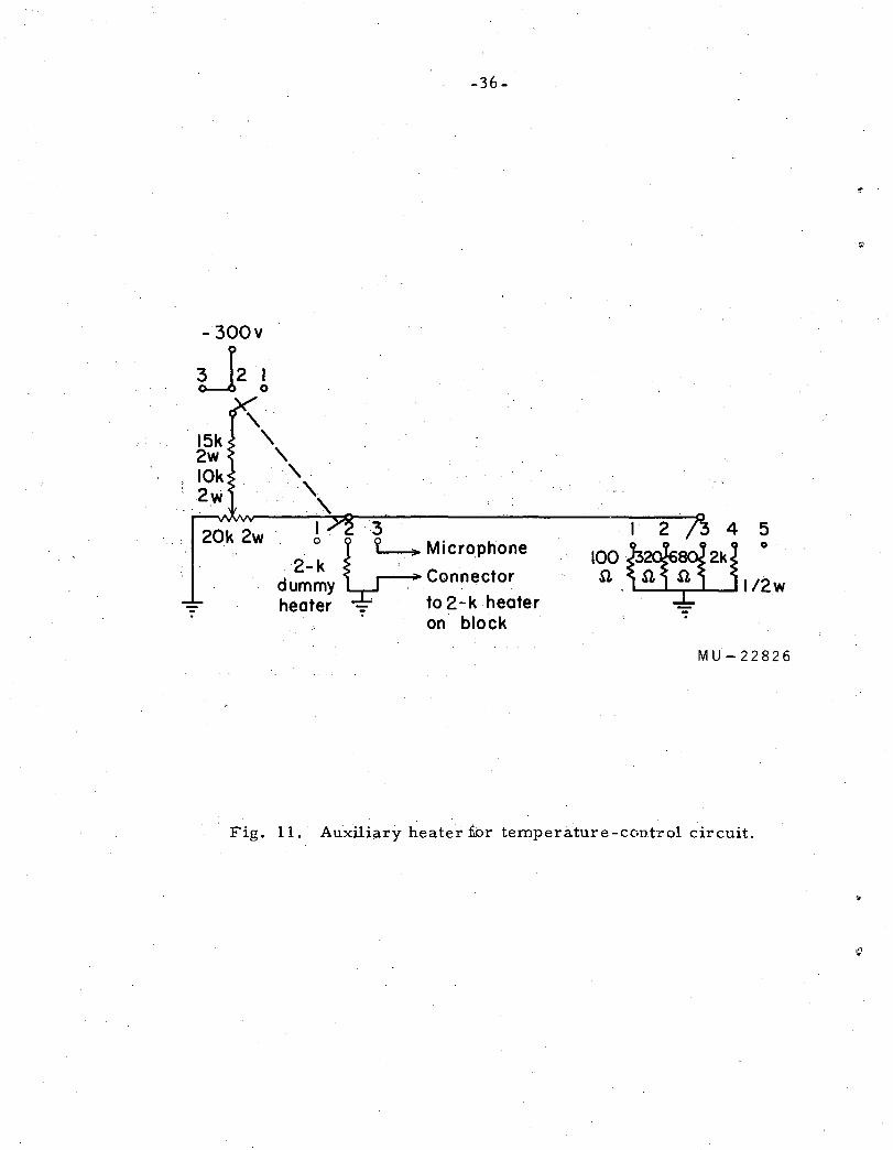
Fig. 11. Auxili~ry heate'r £or temperature-control circuit.

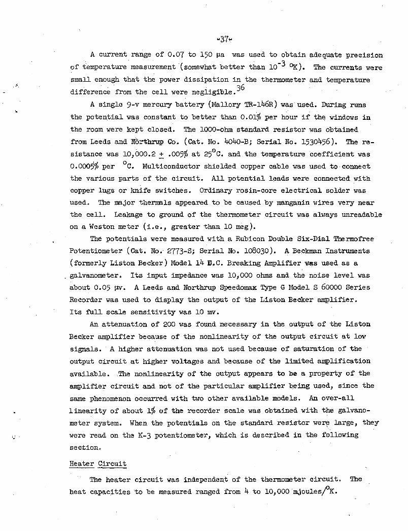
A current range of 0.07 to 150 ~a was used to obtain adequate precision

of temperature. measurement (somewhat better than 10-3 ~). The currents were

small enough that the power dissipation in the thermometer and temperature

difference from the cell were negligible. 36

A single 9-v mercury battery (Mallory TR-146R) was used. DUring runs

the potential was constant to better than 0.01% per hour if the windows in

the room were kept closed. The 1000-ohm standard resistor was obtained

from Leeds and Northrup Co. (Cat. No. 4o4o-B; Serial No. 1530456 ). The re-ar. 0 sistance was 10,000.2 .::!:. .0057o at 25 c. and the temperature coefficient was

o.ooo5% per °C. Multiconductor shielded copper cable was used to connect

the various parts of the circuit. All potential leads were connected with

copper lugs or knife switches. Ordinary rosin-core electrical solder was

used. The major thermals appeared to be caused by manganin wires very near

the cell. Leakage to ground of the thermometer circuit was always unreadable

on a Weston meter (i.e., greater than 10 meg).

The potentials were measured with a Rubicon Double S:Lx-Dial Thermo free

Potentiometer (Cat. No. 2773-S; Serial No. 108030). A Beckman Instruments

(formerly Liston Becker) Model 14 D.C. Breaking Amplifier was used as a

galvanometer. Its input impedance was 10,000 ohms and the noise level was

about 0.05 p;v. A Leeds and Northrup Speedomax Type G Model S 60000 Series

Recorder was used to display the output of the Liston Becker amplifier.

Its full scale sensitivity was 10 mv.

An attenuation of 200 was found necessary in the output of the Liston

Becker amplifier because of the nonlinearity of the output circuit at low

signals. A higher attenuation was not used because of saturation of the

output circuit at higher voltages and because of the limited amplifiCation

available. The nonlinearity of the output ~ppears to be a property of the

amplifier circuit and not of the particular amplifier Qeing used, since the

same phenomenon occurred with two other available models. An over-all

linearity of about 1% of the recorder scale was obtained with the galvano­

meter system. When the potentials on the standard resistor were large, they

were read on the K-3 potentiometer, which is described in the following

section.

Heater Circuit

The heater circuit was independent of the thermometer circuit. The

heat capac~ties to be measured ranged from 4 to 10,000 mjoules;oK.

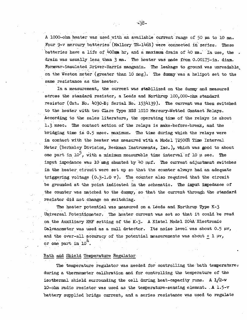
. ' A 1000-ohm heater was used.with an available current range of 50~ to

• . ! I ·. . 10 ma.

Four 9 ... v mercury batteries' (Mallory TR.-146R) were connected in series. . . : '.• .

These

· 'batteries hav~ a life ~f .4o6ma. hr,

drain was usually less than 3 ma. ,. . -: ,,. . .

and a maxim~ drain of' 40 I1R., In use, the ·*

The heater was made from 0.00175-in. diam.

,Formva.r-insulated.- Driver-Harris manganin.

on the Weston meter (greater than 10 meg).

same resistance as the heater.

The leakage to ground was unreadable~

The d~ was a helipot set to the

In a measurement, the current was stabilized on the dummy· and measured

across the standard resistor, a Leeds and Northrup 100,000-ohm standard

resistor (Cat~ No.· 4030-B; Serial No. 1534139 ). The current was then switched

to the heater with two Clare Type HGS 1010 Mercury-Wetted CGntact Relays.

According to the sales literature, the operating time of the relays is about

1.3 msec. The contact action of the relays is make-before-break, and the

bridging time is 0.5 msec. maximum. The time during which the relays were

in contact with the heater was measured with a MOdel 7250CR Time Interval

Meter(Berkeley Division, Beckman Instruments, Inc.), which was good to about

one part in_lo5, with a minimum measurable time interval of 10 J1 sec. The

input impedance was 10 ~g shunted by 4o ll!J.f. The current adjustment switches

in the heater. circuit were set up so that the counter always had an adequate

trigger~ voltag~ (0.?-1.0 v). The counter also required that the circuit

be grounded at the point indicated in the schematic. The inpnt impedance of

the counter was matched to the dummy, so that the current through the standard

res_istor did not change on switching.

The heater potential was measured on a Leeds and Northrup Type K-3

Universal Potentiometer. The .heater current was set so that it could be read

on the AUXiliary EMF setting of the K-3. A Kin tel Model 204A Electronic

Galvanometer was used as a null detector. Its noise level was about 0.5 llV,

and the over-all accuracy of the potential measurements was about ~ 1 llV, . ' ... ·, 4.

or on~ part in_lO.

Bath and Shield Temperature Regulator

The temperature regulator was needed for controlling the bath temperature~

during a thermometer calibration and for controlling the temperature of the

isothermal shield surrounding the cell during heat-capacity runs. A 1/2-w

10-ohm radio resistor was used as the temperature-sensing element. __ A 1.5-v

battery supplied bridge curre~t, and a series resistance was used to regulate

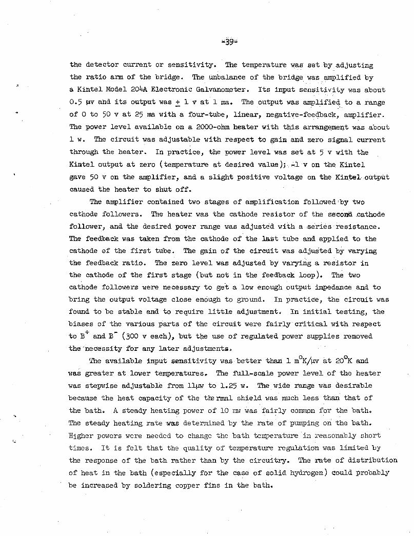
the detector current or sensi ti vi ty. The temperature wa1:r set by adjusting

the ratio arm of the bridge. The unbalance of the bridge was ,amplified by

a Kintel Model 204A Electronic Galvanometer. Its input sensitiv:ity was about

0.5 ~v and its output was + 1 v at 1 ma. The output was amplified to a range - ' ·~-

of 0 to 50 v at 25 ma with a four-tube, linear, negative-feedback, amplifier.

The power level available on a 2000-ohm heater with this arrangement was about

1 w. The circuit was adjustable with respect to gain and zero signal current

through the heater. In practice, the power level was set at 5 v with the

Kintel output at zero {temperature at desired value); ""'1 v on the Kintel

gave 50 v on the amplifier, and a slight positive voltage on the Kintel output

caused the heater to shut off.

The amplifier contained two stages of amplification followed by two

cathode followers. The heater was the cathode resistor of the second .cathode

follower, and the desired power range was adjusted wfth a se'r:i.es ·resistance.

The feedback was taken from the cathode of the last tube and applied to the

cathode of the first tube. The gain of the circuit was adjusted by varying

the feedback ratio. The zero level was adjusted by varying a resistor in

the cathode of the first stage (but not in the feedback loop). The two

cathode followers were necessary to get a low enough output impedance and to

bring the output voltage close enough to ground. In practice, the circuit was

found to be stable and to require little adjustment. In initial testing, the

biases of the various parts of the circuit were fairly critiCal with respect

to B+ and B- (300 v each), but the use of regulated power supplies removed

the·necessity for any later adjustments ..

The available input sensitivity was better than 1 m°K/w at 20°K and

was greater at lower temperatures. The full-scale power level of the heater

was stepwise adjustable from 111-LW to 1.25 w. The wide range was desirable

because the heat capacity of the tm rma.l shield was much less than that of

the bath. A steady heating power of 10 ntvl was fairly common for the bath.

The steady heating rate 'Was determined by the rate of puniping on the bath.

Higher pmvers were needed to change the bath temperature ·in reasonably short

times. It is felt that the quality of temperature regulation was limited by

the response of the bath rather tban by the circuitry. The rate of distribution

of heat in the bath (especially for the case of solid hydrogen) could probably -· .

be increased by soldering copper fins in the bath.

-40-

. Thermocouples

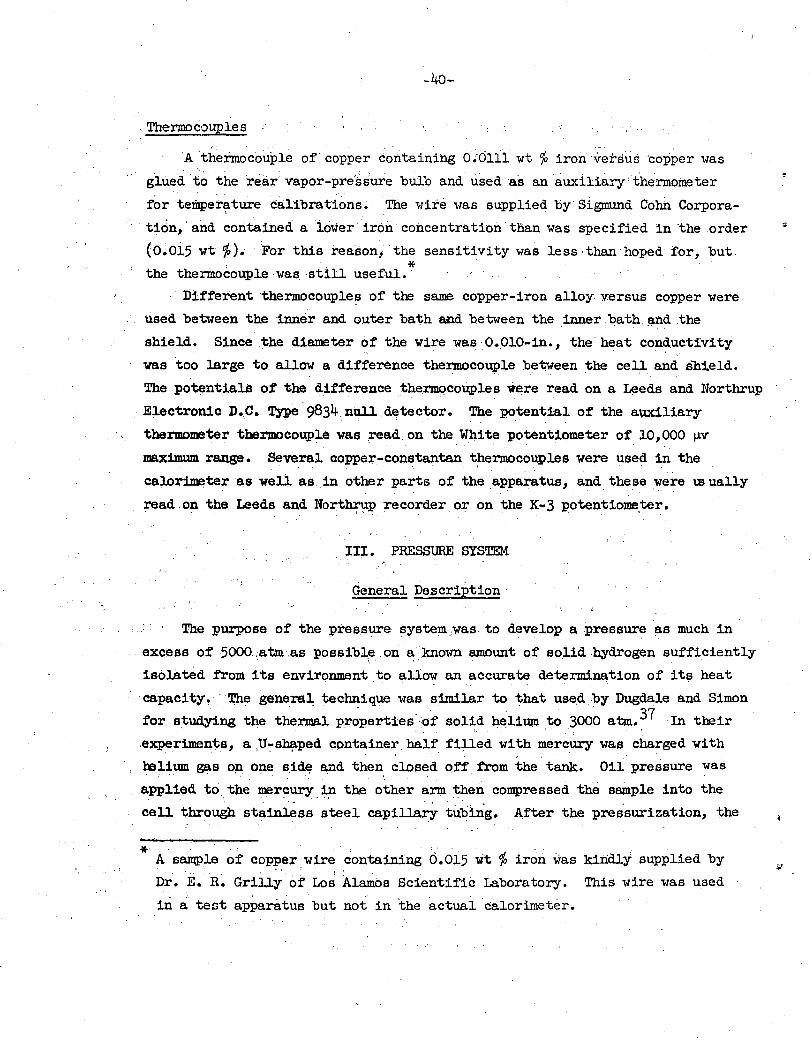
A thermoco~ple of copper containihg O~Olll wt % iron versus ·copper was

glued·t~ the 'rear vapor-pressure buib and used as an'auxiliary•thermometer

for temper~ture calibrat·i.ons. The wire was supplied by Sigmund Cohn Corpora­

tion,· and contained a iower iron concentration· than was specifie'd in the order

(O~Oi5 wt r{o). ··For this reason; the sensitivity was less ·than hoped for, but . . * the thermocouple was ·still useful. ·

Ilifferent thermocouplef3 of the same coppe:r-iron alloy versus copper were

used between· the inner and outer bath aild between the ,inner qath ~il.d the

shield. Since the diameter of the wire was 0.010-in., the heat conductivity

was too large to allow a difference thermocouple between the cell an~ snield.

The po~ntials of the d.ifference thermqcouples .were read on a ~eds and Northrup

Electronic D •. c. Type 9834 null detector. The potential of the auxiliary

'· thermometer thermocouple was read on the White potentiometer of 10, 000 f.LV

maximum range. Several copper-constantan thermocouples were used in the

calorimeter as well as in other parts of the .apparatus, and. thE)Se ."Ylere \.B ually

read on the Leeds and Northrup recorder or on the K-3 potentiometer. ' .. '' - '·

III. PRESSURE SYSTEM

General Description ·

The purpose of the pressure system was to develop a pressure 11s much in

excess of 5000 .atm .as possibl,e on 9: .known amount of solid hydrogen sufficiently

isolated f'rom its environment to allow .an accurate determination of its heat

capacity! ·'The general: technique was similar to that use.d by Dugdale and Simon

for studying th,e thermal pr~pert:l:es· of solid h~lill:!ll t~ .3000 atm. 37 In their

.. experiments, a ,U':"s~ped container half. filled with mercury was charged with

mlium gas op one sid~ and then closed off f'rom the tank. Oil pressure was . . applied to the mercury in the other a~ then compressed the sample into the

. ' t. . --:· ' • . ·.

cell through stainless steel capillary tu~ing. After the pressurization, the

*' A sample of copper wire containing 6. 015 wt % iron was kindly supplied by

Dr. E. R~ Grill~ ot Lo~ Al~s Scientific Laboratory. This wire was used

in a test apparatus but not in the actual 'calorimeter.

helium was frozen in the capillary; and the .sample in the cell was cooled

and f'rozen at constant volume.

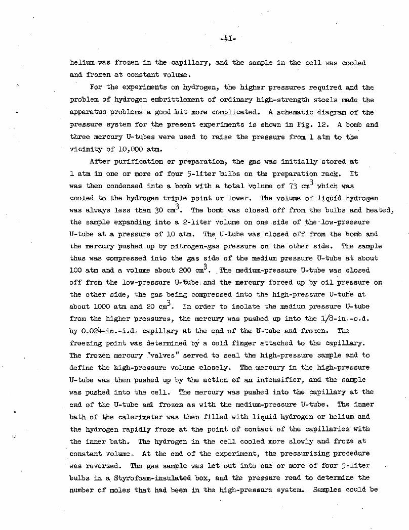
For the experiments on hydrogen, the higher pressures required and the

problem of hydrogen embrittlement of ordinary high-strength steels made the

apparatus problems a good bit more complicated. A schematic diagram of the

pressure system for the present experiments is shown in Fig. 12. A bomb and

three mercury U-tubes were used to raise the pressure from l atm to the

vicinity of 10,000 atm.

After purification or preparation, the gas was initially stored at

1 atm in one or more of four 5-liter bllbs on tm preparation rack. It

was then condensed into a bomb with a total volume of 73 cm3·which was

cooled to the hydrogen triple point or lower. The volume of .liquid hydrogen

was always less than 30 cm3. The bomb was closed off from the bulbs and heated,

the sample expanding into a 2-liter volume on one side of ,the·low-pressure

U-tube at a pressure of 10 atm. The U-~ube was closed off from the bomb and

the mercury pushed up by nitrogen-gas pressure on the other side. The sample

thus was compressed into the gas side of the medium pressure U-tube at about

100 atm and a volume about 200 cm3. The medium-pressure U-tube was closed

off from the low-pressure U-'tube; and the mercury forced up by oil pressure on

the other side, the gas being compressed into the high-pressure U-tube at

about 1000 atm and 20 cm3• In order to isolate the medium pressure U-tube

from the higher pressures, the mercury was pushed up into the ~/8-in.-o.d.

by 0.024-in.-i.d. capillary at the end of the U-tube and frozen. The

freezing point was determined by a cold finger attached to the capillary.

The frozen mercury "valves" served to seal the high-pressure sample and to

define the high-pressure volume .closely. The ·mercury in the high-pre:?sure

U-tube was then pushed up by the action of an intensifier, and the sample

was pushed into the cell. The mercury was pushed into the ~apillary at the

end of the U-tube ani f'rozen as with the medium-pressure U-tube. The inner

bath of the calorimeter was then filled with liquid hydrogen or helium and

the hydrogen rapidly f'roze at the point of contact of the capillaries with

the inner bath. The hydrogen in the cell cooled more slowly and froze at

constant volume. At the end of the experiment, the pressurizing procedure

was reversed. The gas sample was let out into one or more of four· 5-li ter

bulbs in a Styrofoam-insulated box, and tre pressure read to determine the

number of moles that had been in the high-pressure system. Samples could be

From preparation

puri?fcotion Stvrofoom~lined box

-m~;~;;~-;.:;~1---t---~-------lo-40,000 psi ~ 1

5-liter col_ibroted bulbs f~r To orlho-poro 6) 1-~------J Tee Splug

sample determmat1on anol~zer

Mano~eter

{Vacuum manifolds not shown) Oil-valve box

30,000psi

"0-40,000 psi

volume

Fig. 12. Schematic of pressure system.

"

Intensifier 200,000 psi

MUB-625 .·

tl

I fl:>. N

'.

taken for the ortho-para analyzer before or after a pressurization. A more

detailed description of the various parts of the pressure system is given

below.

Low-Pressure System

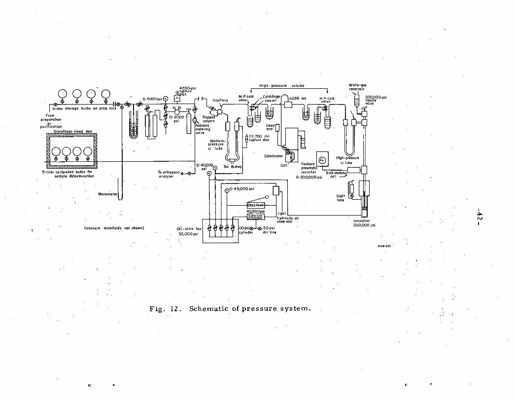
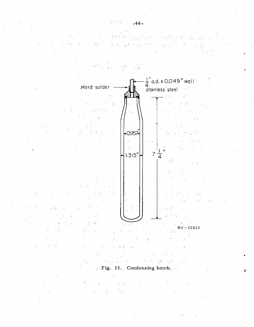
Condensing Bomb

The bomb shown in Fig. 13 was of welded nonmagnetic stainless steel

construction. It was connected to the manifold by 1/4-in.-o.d. by 0.049-

in.-wall type 304 stainless steel tubing and was pressure tested to 5000

psi. The boln.b was cooled in a glass double dewar arrangement equipped for

use with liquid hydrogen or helium. A heater consisting of 27 ft of No. 24

insulated manganin wire with a total resistance of 20 ohms was wrapped around

tlhe outside of the bomb and baked on with formvar enamel. Enough voltage

was supplied to give a maximum heat input of about 15 M. The temperature of

the bomb could be determined by a thermocouple or by the bath vapor pressure.

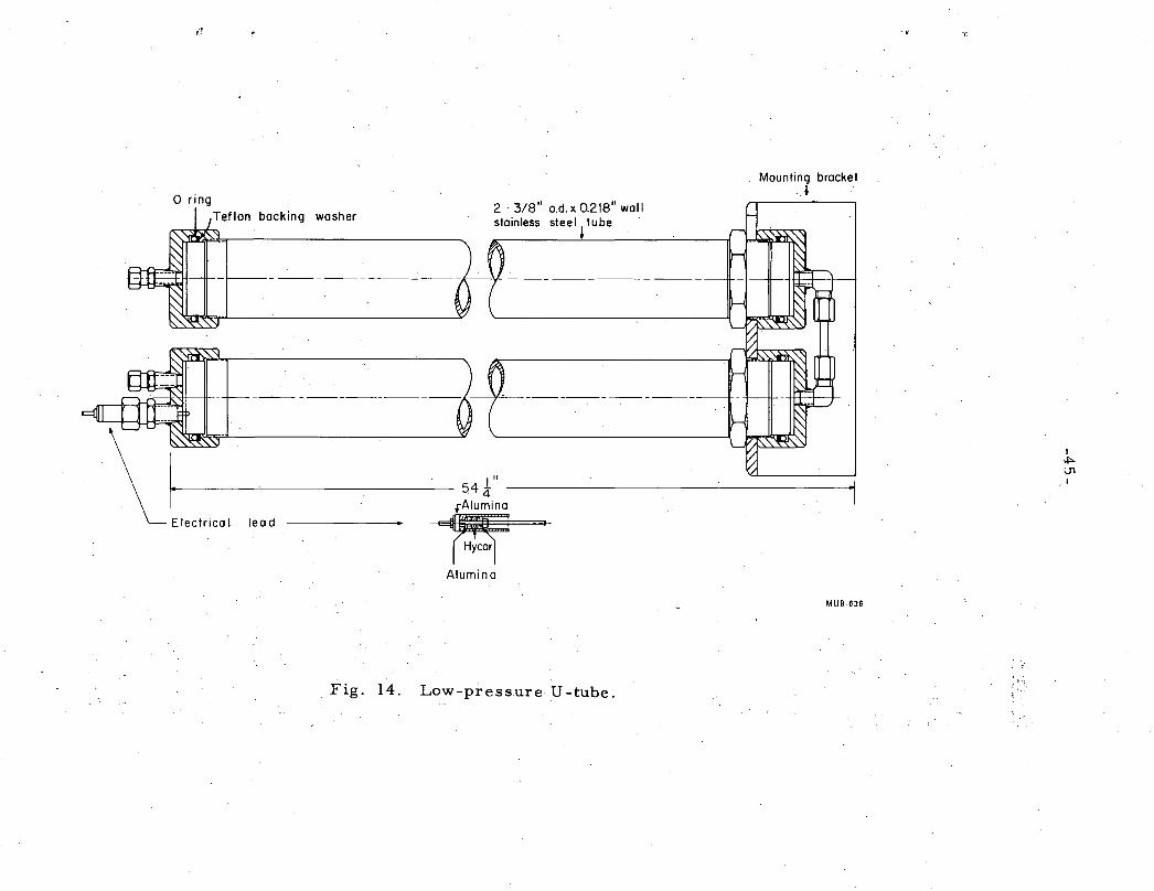
Low-Pressure U-tube

Two 52-in.-long o.d. by 0.218-in. wall stainless steel tubes formed the

arms of the U-tube as shown in Fig. 14. Heavy stainless steel caps screwed

over the ends and were sealed with 0-rings. Parker fittings were used to

connect the caps to 1/4-in. -stainJ.es.s steel tubing. The bottoms of the two

arms were connected by 1/4-in.-o.d. by 0.049-wall stainless tubing. An

electrical lead assembly was fitted into one of the top caps and the U~tube

assembly was tested to 5000 psi. The U-tube was half filled with mercury, '

and the level followed by measuring the capacitance of a Formvar-insulated

No. 16 copper wire suspended from the electrical connection and supported

by the sides of the U-tube. The circuit used to make the depth measurement

is discussed later in the Mercury-Depth Indicator section. The hydrogen

sample was compressed in one arm of the U-tube by pressurizing the other

side with nitrogen gas from a tank connected through a regulator adjustable

from zero to tank pressure. The danger of mercury getting ip.to the manifold

was reduced by having a valve at the top of the U-tube which could be quickly

closed until the driving pressure was released. An indication that the mercury

was near the top was provided by a shorting wire glued to the Formvar of the

depth-gauge wire.

-44-

,Hard solder

I ll ·II ·

- o.d. x 0.049 wall· 4 . I ·stainless stee

I II

7-4

MU-22824

F . 13 Condensing born_. b. . lg. .

..

,,;

backing washer

E lectrica I lead

2 · 3/8" o.d.x0.218" wall stainless steel' tube

I II

54 4

·1!f -Alumina

Fig. 14. Low-pressure U -tube.

Mounting bracket . ~

MUB-626

•~t '('

I

*"" Ul , I

1 Low-Pressure Manifold

Up to the bomb, l/4-in.-o.d. by 0.049-in.-wall stainless tubing was used

and 1/4-in.-o.d. by l/16-in.- i;~:d. -~:o.bing ·.was· use..d b'eyond ·;,:theL bomb .• _ ·:American

Instrument Co. parts used in the low-pressure manifold included "quick-connect"

:flareless fittings, valves (Cat. No., 44-1203), and a blowout assembly (45-9011}

with a rupture disc to hold 4200 psi. The valves had 0-ring seals on the stems

and were helium leak-tight at 2000 psi throllgh the stems and seats. A 0 to

5000-psig (47-8205) was attached to the low-pressure'manifold for operational

pw:q>oses. Several metering Valves were· tried for. t:l:ie p\tl:'pose of letting the

gas from the tank at 100 atm into the evacUa.ted 5-liter bulbs.·. The most

satisfactory was a stainless steel· type ·with a KelaF seat and an 0-ring stem

s.eal made by Robbins Aviation Co. (INS G 103-lP).

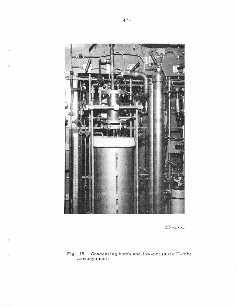
The condensing bomb, low-pressure U-tube, and manifold are shown in

Fig. 15.

Mercury Depth Indicator

Initially it was hoped to follow the depth of the mercury in the U-tubes

by measuring the resistance of a wire supported in the tube. Stainless steel

wire was tried, but the mercury deposited a layer of insulating material on the

wire vfu.ich made the resistance measurement· very erratic. ·.The effect was

apparently due to an interaction between the mercury and the steel, and ·did

not seem to depend on the initial cleanliness of the mercury. A similar effect

was observed by Bridgman. 38

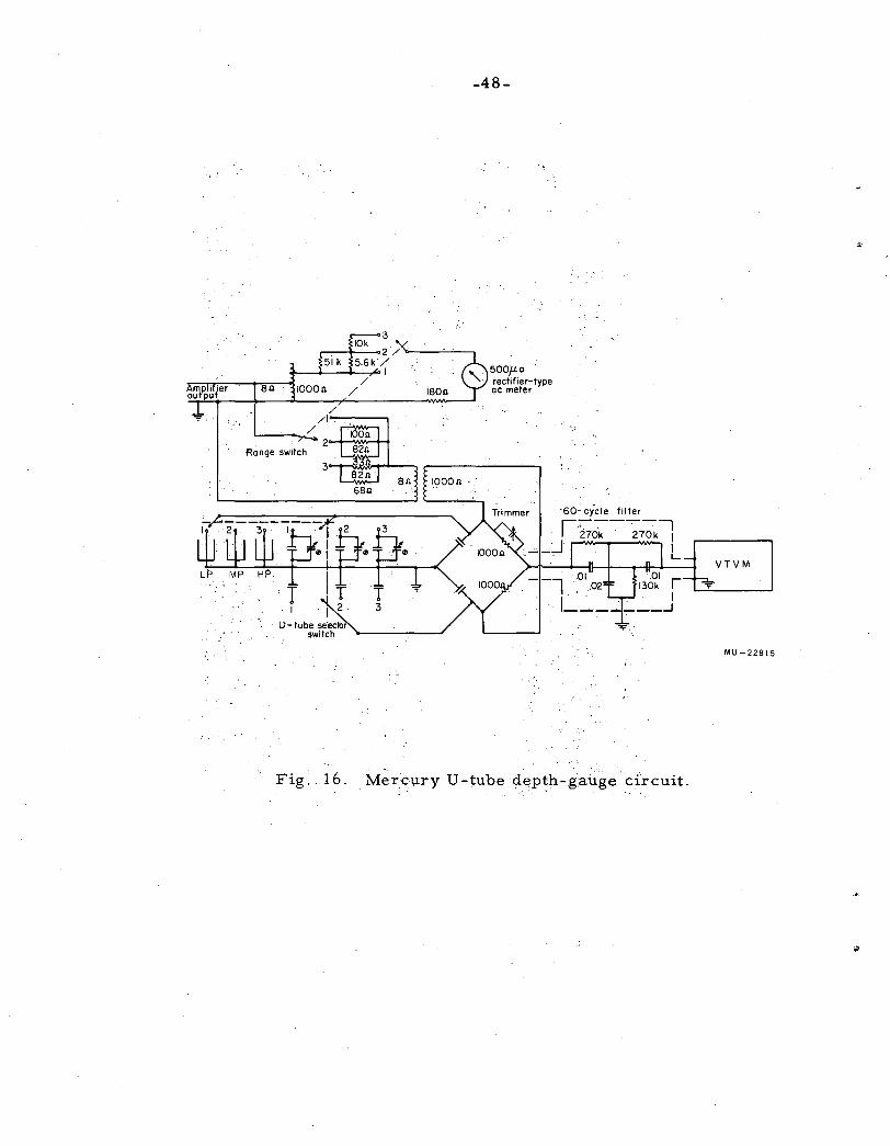
. In order to avoid this problem, it was decided to measure the capacitance

of a Formvar-insulated copper wire suspended in the mercury. The internal

diameters of the low-, medium-, and .high-pressure U-tubes were 2 in., 5/16 in.,

and l/8 in., respectively. The lengths of the. depth gauges were made 4 ft,.

12 ft, and 160 em, respectively. Number 16 (51-mil) wire used in the low­

pressure U-tube and No. 20 (32 mil) was u.sed in tl;le medium- and high-pressure ..

U-tubes. The thickness of the Formvar insulation was measured and found to be

1.6 mils. By taking the dielectric constant of Fori:nvar as 3.12 and using the :;

expression for the capacitance of a cylindrical condens~r, the sensitivity of

· the low-pressure U-tube was roughly estimated to be .29 f.l.P.f/cm and that of the

medium- and high-pressure U-tubes to be 18 pf.l.f/cm. The circuit is shown in

Figure 16. The capacitance of the wire was made lr:J{o of that of one arm of

-47-

Z N - 2732

Fig . 15. Condensing bomb and low-pressure U-tube arrangement.

.-,:

3

-48-

500"fLO rectifier-type ac meter

Fig. 16. . Mercury U -tube ·dep~h-g'auge circuit.

VTVM

MU-22815

-49-

a Wheatstone bridge. The depth of the mercury was indicated by the unbalance

of the bridge, which deviated about 5% from linearity at full-scale unbalance.

Three sensitivities" were incorporated: low, medium ( 4x), and high (lOx). A

General Radio 1-kc tuning-_fork oscillator was used with a 10-w high-fidelity

audio amplifier to power the bridge. A Triad S-25Z Autoformer and a Triad

S-78Z Output Transformer were connected in parallel to the output of the

amplifier, the former to supply current to a,Weston 500-IJ.S. rectifier-type

ac ammeter, and the latter to isolate the bridge from the meter and the

sensitivity switch. A shielded 60-cycle. twin-T filter was found necessary

at the input of the detector, a Shasta vacuum-tube voltmeter. The bridge

current was adjusted by setting the meter to 220 pa with the amplifier gain

control, and the vacuum-tube voltmeter was used on the 10-mv scale. Adjustment

of the bridge zero was provided by 200-~~f screwdriver-actuated capacitors on

the front panel for the three U-tubes. The bridge was not accurate enough to

give quantitative indications of the mercury depth, but was an indispensible

aid in operating the U-tubes.

Shielding

The part of the pressure system involving gas above 100 atm was largely

enclosed in 1-in.-thick mild-steel plate. The general features of the shield

are shown in Fig. 17. The design was based on information available to us

concerning safety features desirable with high pressure apparatus.39 The main

working area in the shield was a 3-ft-wide, 4-ft-high, and 18-in.-deep box

with sliding doors on both sides. The sliding doors moved on roller bearings

and proved to be very convenient. A small welqed 1/2-in. steel box was also

included in the shield for pressure testing the cells. The box was just

large enough to hold. a quart dewar. The medium~ and high-pressure U-tubes

extended from the bottom of the box through a trap door to the floor below.

They were enclosed in a 1-in.-thick by 14-in.-diam. steel pipe to the bottom . .

of the high-~ressure U-tube, and in 1/2-in. steel pipe to the bottom of the

medium-pressure U-tu.be. A 1/2-in. -thick steel box shielded the bottom of the

medium-pressure U-tube and provided access to the fittings .there. The medium­

pressure U-tube was assembled in the 1/2-in. shielding and then pulled into

the shield from two floors down through a second· trap door. Th.e high-pressure

U-tube was lowered into the shield through a trap door from the floor above

before the roof of the shield was installed. The bottom of the calorimeter

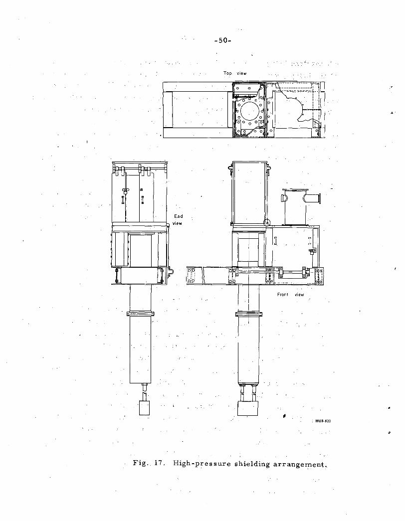
pmJ r- rrru- l

s p Cil

n n

u ]

..

u

Fig. 17.

-50-

Top. view

End

v iew

~

: ',. ''.! ~ • . . . :.

------ --------,r-\1 =~~~~~;;~~-~~--~

I I I I I''[

: I I I

MUB-6ll

High-pressure shielding arrangerpent.

a·

was also shielded with l~in~ steel plate which was attached to the side of

the box containing the high-pressure fittings. The shielding and .. .enclosed

equipment weighed about 5 tons and were supported by two 12-in. · steel I~beams

which rested on two of the concrete beams in the floor.

Medium-Pressure System

Twp oil pumps were used: an air driven one for handling the large volumes

required by the medium-pressure U-tUbe and the intensifier~ and a hand pump

for the slow movement needed when pushing the mercury into the capillaries.

The air-driven pump was made by the Sprague Engineering Corporation, whose

designation was s~44o-200. About 100 psi of air were required to generate

an output of 20,000 psi in the oil. The pump maintained the pressure to which

it was set, and had a capacity of more than 300 cm3 /min -- much more than

required. A 50-psi house air line was used for pressures up to about 11~000

psi, and a cylinder of compressed air was used for higher pressures. The

hand pump was a Blackhawk Model P-228; rated for use to 4o,ooo psi. At low

pressures its stroke was rated at 0.4 cm3, ?ut was smaller above io,ooo psi.

For the 0-20,000 psi oil sys:tem 1/4-in.-o.d. by 1/16-in. i.d. tubing was used

with American Instrument Co. connectors (45-1310). American Instrument valves

(44-3105) rated to 30,000 psi were used in the oil manifold. A rupture-disc

assembly ( 45-9103) was used in the medium-pressure U-tube line with a disc

. to hold up to 22,500 psi. Blackhawk LX-21 hydraulic oil was used in the pumps,

medium-pressure U-tube, and low-pressure part of the intensifier.

Originally it was thought that fairly short large-diameter cylinders would

be used to separate the hydrogen from the 6il. The cost of constructing these

parts from metals resistant to hydrogen embrittlement would have been quite

high and, in the case-of failure, the cost of replacement would have been

equal to the initial expenditure. After consultation with Mr. Donald H.

Newhall, Pre.sident of Harwood Engineering Co.~ it was decided to use very

long small-diameter composite tubing for both the medium-pressure and high­

pressure systems. Although the use of these tubes raised space and installa­

tion problems, the much lower initial and replacement cost made their use

worthwhile. The composite tubing consisted of stainless steel jacketed with

alloy steel.

·-52"'

The medium-pressure U-tube, for use to 20,000 psi, was 15/16-in.-o.d.

by 5/16-in. Ld. Each arm was a separate piece 14 ft,. 8 in., long •. The length

of the straight portion was about 13 ft, 9 in. Harwood Engineering Co. 15LH

type fittings were used to connect the U-tube to the rest of the system. The

sealing elements to the tubing were lens rings. A tee with a cap was put at

the bottom to join the two arms. During the bending of the tubing, the jacket

stretched. over the inner stainless tube by a small amount at the lower end.

The angle on the lens ring was great enoUgh to keep the seal on the inner

tube, but in tl'le tighteningJ the outer tube was pulled further over the inner

one and on one side of the U•tube the seal shifted to the outer tube. This

effect was not discovered until mercury had been forced all the way up the u~

tube between the two layers. of metal and out at the top. The difficulty was

remedied by refacing the end of a new tube after it' had been bent to the

proper shape.

The oil was brought into the U-tube through a tee at the top. An electrical

lead was brought in through the top of the tee on the oil side. A lava cone

was used as the insulating seal. The dimensions of the electrical lead are

shown in Fig. 18. Originally it was hoped to have the electrical lead on

·· the gas ~ide, but the cone could not be made leaktight against helium.

Several attempts were made with the cone lightly coated with rubber cement •.

A thin layer of red iron oxide was also tried but the helium leak rate was

a1ways unacceptableo Although switching the· lead to the oil side :ma'de the

indication of the mercury level on the gas side more indirect, it solved the

critical leak problem, and also eliminated one of the trapped volumes in the

gas system. As shown in Fig. 19, 1/4-in.-o.d. by 1/16-in.-i.d. tubing was

connected to the top of the U-tube on the gas side. This tubing sloped

gradually upwards to a tee, one arm of which was connected to a valve for

closing ·Off the low pressure system. The other arm was adapted to 1/8-in.­

o.d. by 0;;024-in.-Ld. hard-drawn stainless steel capillary tubing leading

to the high-pressure·system. The arm ieading to tlie valve constituted the

only trapped volume in the gas system. The capillary tubing was arranged

.•

to come out the top of the tee so that any droplets of mercury coming over #

from the low-pressure system would tend to go into the U-tube•

The mercury-depth indicator consisted of a 12-ft piece of'No. 20 Formvar­

insu1ated wire. The end was coated with GE 7031 cement which was baked on to

give chemical resistance to the hydraulic oil. A thin stainless steel wire

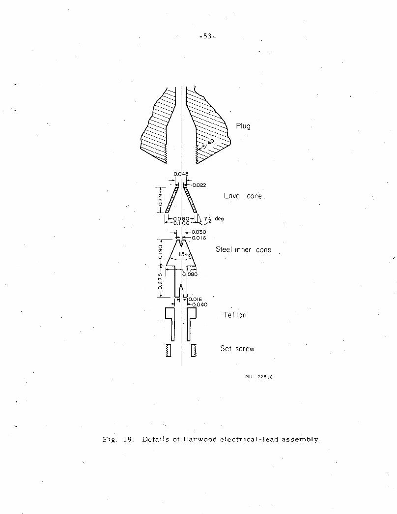
-53-

Ijf\022 11-o.oso...J 1\ 7~ deg ~0.106~

Plug

Lava cone

-1 I 1-- o.o3o d +11

14--0.016

m Steel inner cone d

+ I()

1'­N

d _L_

1 ~ 1410.016 ~ '-0.040

·.~'? n I a

I

Teflon

Set screw

MU- 22818

Fig. 18. Details of Harwood electrical-lead assembly.

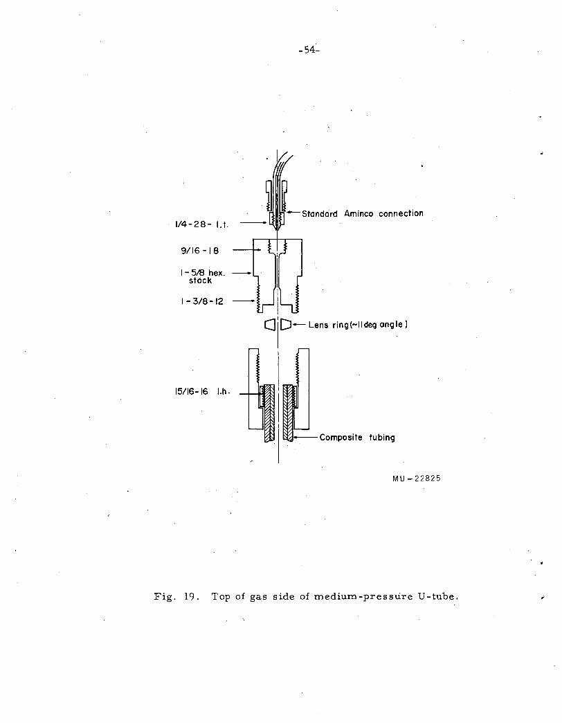
1/4-28- l.t.

9/16-18

1-5/8 hex. -stock

1-3/8-12

15/16- 16 l.h.

-54-

Aminco connection

cJ i D- Lens ring(- II deg angle I

I

-Composite tubing

MU-22825

Fig. 19. Top of gas side of medium-pressure U-tube.

was soldered to the lead at the top and gluedto the copper wire so that its

end was several inches below the side arm of the tee on the oil side. Its

purpose was to short the indicator when the mercury ·Was in danger of ·going

back into the oil system. It was easy to tell when the mercury went off

the low end of the wire because the indicator stopped moving. The medium­

pressure depth indicator was set up so that the bridge was balanced when

the mercury was all of the way up on the gas side, hence the highest sen­

sitivity could be used to determine when the mercury went off the end of the

wire. The mercury level was adjusted so that it was at the top of the U-tube

(within a few em) on the gas side at 1 atm when it was at the end of the wire

on the oil side.

After reaching the end of the U-tube, the mercury was pushed up into

the smaller tubing, through two arms of the tee, and into the capillary

tubing. This operation was carried out with fairly slow strokes of the

Blackhawk pump. Upon reaching the cold finger-heater arrangement clamped

to the capillary, the mercury froze. The purpose of the heater was to give

a sharp temperature gradient at the cold finger in order to fix the freezing

point of the mercury more closely. The temperature of the capillary under

the cold finger was about -80°C. and the temperature under the heater was

about room temperature. Mercury freezes at -39°C. The motion of the,_mercury

in the capillary was monitored with a copper-constantan thermocouple soldered

just past the cold finger. Before the mercury froze, each stroke of the.pump

caused gas to rush through the capillary at the thermocouple, giving a slight

but sharp temperature rise (about 0.1 mv under typical conditions). This

signal was amplified by a factor of ten and displayed on a recorder. The

freezing of the mercury at the cold valve was then indicated by the lack

of response of the thermocouple to further strokes of the Blackhawk pump.

This technique worked well except when there was a leak in the high­

pressure system beyond the cold finger. Then the presence of the trapped

gas volume seemed to cause a mixture of mercury and gas to be pushed into

the capillary. Application of higher pressure on the other side after freezing

the cold valve behind the cold finger then usually pushed the mercury back,

probably because there was not enough frozen to make a gpod plug. It was

found necessary to lower the cold-finger dewar after freezing the cold valve.

This left a puddle of liquid which then filled in the cracks formed by the

contraction of the mercury on freezing. When the mercury was pushed up to

the cold finger slowly enough,)) it seemed·to freeze .before getting past the

cold finger. Evidence for this was given by the fac~·tl1at a slight release

of pressure caused the plug to break and move back. On the,other hand, if

the mercury was moved up to the cold finger with full sharp strokes of the

Blackhawk, it did not. unplug when th~ pressure was released sl~ghtly. Since

the cell was made of a copper alloy, :it had to be protected from mercury

contamination. For this purpose a U-tube was put in the capillary past the

cold finger and maintained at acetone--dry-ice temperature. Experience

indicated that this protection was necessary and adequate.

High-Pressure System

A single piece of 3/4-in~-o.d. by 1/8-in.-i.d. composite tubing was

bent into the proper shape. The total depth of the U-tube was 10 ft. A

Harwood Engineering Co e A-2• 5J intensifier was used as a source of pressure.

Its range was 0 to 200,000 psi output for 0 to 15,000 psi input. The high­

pressure stroke was 20.l-cm3• The volwne on top of the low-pressure piston

was 303 cm3• It was. filled with hydraulic oil and connected to a sight tube

for the purpose of indicating the position of the piston. The large ratio

of volumes (15:1) made it very sensitive. Whif,ja. gasoline was used in the

high-pressure system. Hydraulic oil was used in the low-pressure side, and

the Sprague and Blackhawk pumps were used to pressurize the in·tensifier.

Some tro~le was experienced with the packing of the high-pressure

piston. A wax-impregnated leather washer contained by triangular cold­

rolled steel washers was used. During shipment, the wax had dissolved out

of the packing and it could not be made leaktight. A plastic i1npregnated

washer was tried, and this proved ·satisfactory after it had been pressurized

a few timeso The intensifier was dead-ended and pumped up for the purpose

of breaking in the new washer. The :manner of connecting the intensifier to

the U-tube is illustrated in Fig. 10. Harwood type-12H fittin~~ were used.

The pressure~~asuring cell was connected to a tee directly above the . .

intensifier. It was supplied by the Harwood Engineering Co. Its principle

.•

of operation involved the bulk compression of a steel rod which was connected

by a probe to a pneuma tic system manufactured by the Foxboro Coo The pressure

was read on a recorder driven by the pneumatic systemo The recorder could

be read to + 500 psi.

..

.;.57.;.'

A l2H valve was included in the white gasoline system for the purpose of

adjusting the amount of fluid. The elec:brical lead was brought in through the

top of the tee on the white-gasoline side._ The -same principle for obtaining

an insulated seal was used as with the lead in the medium-pressure U-tube. The

seal leaked when first pumped to about 4o,ooo psi, but after the pressure was

raised to about 100,000 psi, it was leaktight at all pressures. On the gas

side of the U-tube, capillary tubing was connected directly to the top of the

u-tube with the arrangement shqwn in Fig. 20. The method of connecting the

capillary tubing was described by Paul and Warshauer. 4o Th~ high-pressure

u~tube, medium-pressure-U-tube, and cell were connected together by a tee made

from Allegheny Ludlum A-286 stainless steel, which was required by the presence

of hydrogen and mercury. All of the Paul-and-Warshauer fittings were also made

of A-286. The sealing surfaces of the fittings galled badly and had to be re­

faced periodically. A cold· finger, cold valve, heater, and acetone-dry-ice

trap identical to those used in the medium-pressure system were used between

the top of the high-pressure U-tube and the A-286 tee. The 1/8-in. holes in

the tee were stuffed with gold foil to .act as a quick indicator of the presence

of mercury.

The filling of the high-pressure system with mercury and white gasoline

was not as trivial an operation as with tre medium-pressure system because the

compression of both the white gasoline and mercury at the higher pressures

was a large fraction of the intensifier stroke. In addition, the amount of

white gasoline had to be fixed before the pressurization. The following con­

siderations illustrate the conditions for the maximum stroke of the high­

pressure piston. It was desired to have the mercury 30 em below the top of

the tube on the 'White gasoline side under 1000 atm compression. With the

intensifier all of the way back, the amo~t of white gas in the system was

about 25 ~3 • If we assume a compression of 12% at 1000 atm, the 1-atm

volume of the white gasoline was 28.4 cm3 • Since the cross section of the 2 U-tube was 0.079 em , the mercury was 73 em below the top of the U-tube at

1 atm. On the gas side, it was desired to have the mercury at such an initial

height that it could be pushed to the cold f.inger at the end of the stroke. If

we take the volume of mercury as ab~ut 37 cm3 and the compression between 1000

and 10,000 atm as 3%, the amount of the intensifier stroke that ·went into the

compression of the mercury was 1.1 cm3. T~ing the compression of the white

gasoline as 25% from 1000 to 10,000 atm, 7.1 cm3 of the stroke went into its

compression.- Hence the net high-pressure stroke available for compressing

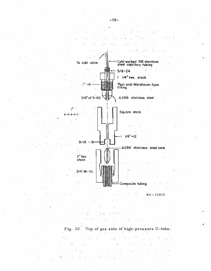
To cold valve

lu

I t I I I

9/16-18

2 11 hex.

stock

3/4-16-l.h.

-58-

-Cold-worked 316 stainless steel capi II a ry tubing ·

I 1/411 hex. stock . •

Pau 1-and-Wa rshauer- type fitting . .

stain less steel

Square stock

MU-22829

Fig. 20. Top of gas side ofhigh-pressure U-tube.

-59-

the hydrogen was 11.9 cm3• Allowing a 10% margin, one finds .that .the mercury

will be about 82 em below the top of the tube at l atm and 126 em below the

top at 1000 atm. By using the above considerations~·· the mercury level was

.adjusted to 78 em below the top of the U-tube ·and checked on -both sides to

make sure that there was no air trapped in the ·mercury. The depth-indicator

wire ·was attached in the same way as in the medium-pressure tube e;x:cept that

the length was 160 em'. Hence when tre mercury . was 10 cin below ·the top on

the gas Side; it left the end of the .wire on the white gasoline side.

It was found that. the Formvar insulation. cracked after being in the white

·gasoline for a while and then. shorted when· the pressure was raised above about

1000 atm. ·The white gasoline seems to have dissolved the plasticizer and made

-the Foi'mva.r brittle. Teflon insulated wire made by American Super-Temperature

Wires, Inc. is now being tried.

High-Pressure Cells

General

The general requirements for the metal used in the high-pressure cell

were high mechanical strength, small heat capacity, reasonable heat conductivity,

resistance to hydrogen ~mbr~ttlemerit:, lack. of magnetization, and resistance to

mercury attack. The only metals which s,eemed to be reasonable 'possibilities

were stainless st~els (cold-worked 316 or A286.) and beryllium copper. The

stainless steels did not match up to the beryllium copper in mechanical

strength or in heat conductivity, although they were not vulnerable to mercury

attack. Since it was possible to eliminate mercury from the cell by JGaking

precautions in the connecting parts, it was decided to use the beryllium-copper

·. alloy. . This material has been used previously for high-pressure vessels. 41

Berylco No. 25 rod was 0btained from the Beryllium Corporation in the

annealed condition~ Itsnominal.composition was 1.8-:2.05%-beryllium, 0.18 to

0.30% cobalt:, a.n:d. the balance copper. The following properties were given in

the supplierss literature. In the annealed (l450°F)·co:ndition, its tensile

strength is 6o,ooo to 8o,ooo psi. · After heat treating• a.t 600°F for 3 hr, its

tensile strength could be raised to about·l8o,ooo psi. .The hardening was

caused by a precipitation process. The yield· strength for 0.1% offset in the

hardened condition was. about 130,000 psi. .The elastic modu;Lus in tension at 0 . ' . ... 0

20 C was 19,000,000 psi. The linear thermal expansion per C in the range 20

to l00°C wa.s 1.67 ;x: 10-5. ·. Poisson's rat;io ~as 0-3,' and the d~nsity increase

-60-

on heat treatment was 0, 6~b.

Thermal Expansion

The thermal expansion of the material. from :the lov1est temperature to

room temperature·. was estimated by ass LUning the tJiermal expansion to be.

proportional t.o the. heat capacity ( Gruneisen 1 s Law). P.reliminary experiments

indicated that the hardened berylliwn coppe:r had a .heat capacity very .similar

to that of copper" for vrhicb QD = 3L~o°K. The proportionality bet;veen tre rmal

expansion and heat capacity was fou..11d at, roorr. tempe.rature, and the change of'

volume vras determined. from available tables cf the integral of 1.he Debye

function. 42

A change in volu."!le of 1.0% from 0 to J00°K vms epi:·imated. This

value compares. favo:rably with SWenson s estimate of 0.9·+ 0.3~~·l.'3 . The volume

change be lov 77°K amount-s to less than 0. l~~.

Pressure and Volume Considerations

During the course of sett-ing up the apparatus, three t;ypes of cell were

made. The first design consisted of a hardened inner cylinder \·li t.h an annealed

cylinder shrunk over. it. The second design had the same dimensions as t.he first

except for a somevrhat larger outside diameter, bu-: was made from a single piece

and hardened. It was made as insurance in case the first design proved unreliable.

Trouble I·Tas experienced in keeping the Bridgman seals leakt.ight during the cool- ·

down on the above designs~ SO a lOH-pressure cell with the ends screwed in and

soft-soldered >·ras c-onst,ructed for the purpose of obtaining ds. ta •·Thile the

technique of sealing the high-pressure cells was being perfected. Dl"a.vlings

of the cells are shown in Fig;r., 21 and 22.

Calculation of Pressure Efd'ects

In t.he follmving consi.de:cat lons., the pressure dividing :elastic .from in­

elastic flm·r is first. calculated, and then the ':Jurs·t pres:::.ure is estimated.

The volwne changes in the elast.tc and plastic reg.i.ons are then estimated and

the uncertainties are 'discussed. 'T'he low-pressure and solid cell a.re considered ·•

first for cross section and longi'tudi.nal stretch. The effect of' the Bridgman-

seal end plugs on the soiid cell is then calculat;ed. The propert.ies of the

composite cell are calculate.d last. The pro-blem of seal.s on the hi.gh-p:r·es.sure

cells is then discussed.·

Pressure Limit for E.lastic Flow

Formulas for calculating the properties of pressure vessels have been

'•

-61-

II" 1------'-------'---'--- 4 i6 ----'--,------'---~

3 ·, - of 16

3" 4

7" I. h . ( - - 2 8 des ira b I e ) 16

MU-22828

Fig. 21. Low-pressure cell.

'

-62-

I"

~---;;-----~ s z4 -------------1

'·'" ~6----~ f ..................... w;;;;;;:;;;;;w

7 ·- 28 A Irs _1_ .,.......,.._. ._. ........ ...,

a. Outer part

= 0

~ f I 1"""~3~~~8~'-· - 4 :.r:~l-0-.-25-0-,-, ~----0~.=28;;;cl;-rr",_.,.

~~======~============~ b. Inner part

part

part

c. Seal (not to scale) MU-22827

Fig. 22, High-pressure cells. (a) Outer part, with A= 11/16 in. for composite cell and 0.730 in. for solid cell; (b) Inner part of composite cell; (c) Seal (not to scale). ·Parts a and b on composite cell have 0.003-in. interference fit.

. 44 discussed by Comings. The most usefUl relations for the present purposes

' have been collected in Appendix B. The largest stresses are 'the tangential

· 0nes a.t the inner radius. If a, permanent volUme increase of o~ifo is taken

as the criterion of elastic behavior, there will be &_,~nt .set of 0.1%

in the radius. If ay is the stress t~t gives the .Permanent offset of 0.1%

in the :f.lnier .. radius (or cireum:ference ); the ~ formUla. gives for zero

(4)

(5)

If we have a = 130,000 psi for 0.1% offset, we can calculate the pressures y

given in .Table IVo

Table IV., Pressure J4mi t for elastic flow

Cell K K2 p a py

b rl r2 y

Low-0·375 0 .. 688 lo83 3·36 70,4oO 52,700 pressure

Solid 0.250 0.730 2.92 8.53 102,800 66,eoo

~ Eq. ( 4). Eq. ( 5 ).

Burst Pressure of Cell Walls

Using the criterion that the cell will burst ~hen the plastic flow ex­

tends to the outer wall, it has been shown that we obtain

(6)

-64-

This :formula ignores strain hardening. Two estiin13.tes are included-­

one :for the yield ~trength (130,000 psi), and the other f~;>r the tensile

strength (180,000 psi). The actual burst pressure prob~bly lies between ' ' . . ' ' ~ ' . .

the two estimates. Estimates o:f the burst pressure are ~iven in Table V. ,., .

Table V. Estimate p:f burst pressure ..

pb p Cell K lnK b

. (130,000) (180,000

Low 1.83 0.605 90,800 126,ooo pressure

-.. , '

Solid 2.92 1.071 161,000 223,000

Volume Cha.nges Below the Elastic Li~ t ,

The radial displacement is given by

(7)

At r 1 with P2

= o, the tangential strain is

- p . 2 _! [ 1- 2v + (1 + v) K J

.E K2 - 1 (8)

Taking E = 1.9 x 107 psi and,) = 0.3, one obtains the percentage increase in

cross section listed in Table VI.

Table VI. Percentage increase in cross section

. K2 ( €t )rl 8A.., ( €t) Cell p --2 rl y

pl A

%

Low 1.06 X 10-7 pressure 50000 3.36 1.1

Solid 65000 8.53 0.81 X 10-7 1.1

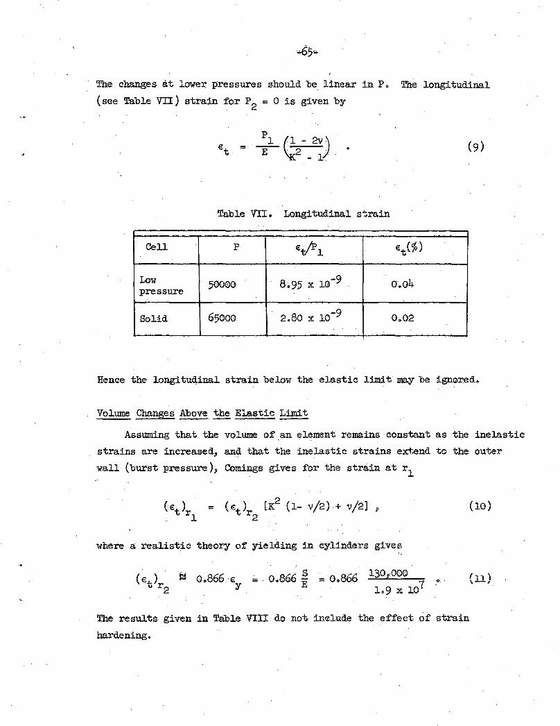
The changes at lower pressures should be linear in P., The longitudinal

(see Table VII) strain for P2

= 0 is given by

p

= + (L- 2V) . y -1." (9)

Table VII.. Longitudinal strain

Cell p eJP . 1 et(ojo)

Low 50000 8o95 X 10-9 o.o4 pressure

Solid 65000 2.80 X 10-9 0.,02

Hence the longituqinal strain below the elastic limit maybe ignored.

Volume Changes Above ~ Elastic Limit

Assuming that the volume of .an element remains constant as the inelastic

strains are increased, and that the inelastic strains.extend to the outer

wall {burst pressure), Comings gives for the strain at r1

2 (et) = ( et) [K (1- v/2) + v/2] ,

. rl r2 .

where a realistic theory of yielding in cylinders gives

( ) ' "" 866 866 s 866 l30pOOO E ~ Oo .E =. 0. • i = 0., · 1

o t r2 y lo9 X 10

The results given in Table VIII do not include the effect Gf strain

hardening.

(10)

(11)

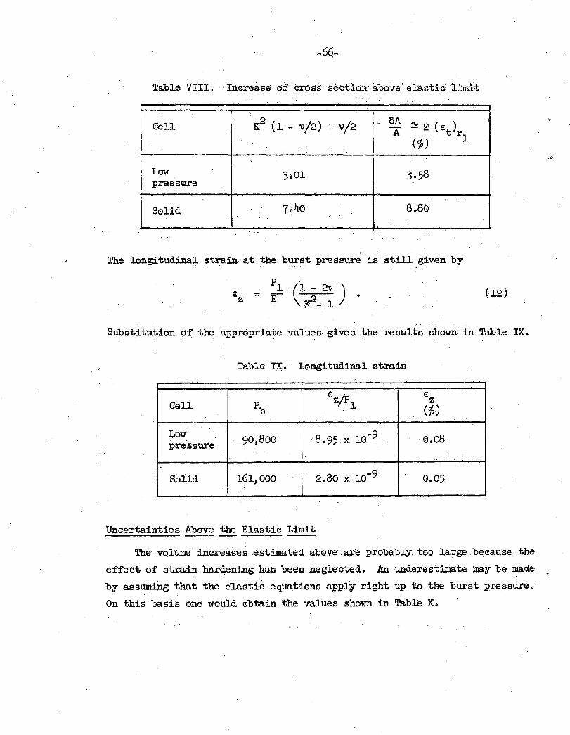
Table VIII. Increase of Cross se'ctiori above ela.s't:l.C l:tndt

Cell ~ (l v/2) + v/2 ~ 5A ~2 (€t) - A (%)

rl :

Low 3·01 3·58 pressure

Solid 7.;40 8o80

' The longitudinal strain at the burst pJ:'essure is still given by

' ' pl (i - 2\1 ) €z = E _2 _ •

K--- l . (12)

Substitution of the appropriate va·lues gives the result~ shown in Table IX.

Table !X. Longitudinal strain -

€/P € z Cell pb z_l

(%)

Low 901800 8.95 10-9 . o.o8

pressure X

·- -

solid 161,000 2.80 X 10 -9 0.05

Uncertainties Above the Elastic Limit

The volume increases estimated above are probably too J.a.rge, because the

effect of strain hs.r<lening has been neglected. An underestimate may be made .

by assuming that the elastic equations apply right up to the burst pressure.

On this basis one would obtain the values shown in Table x .. -.-

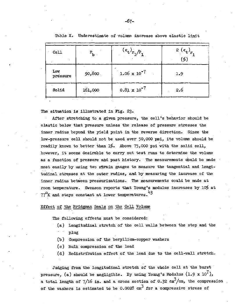
Table X. Underestimate of volume increase above elastic limit

Cell pb (et)rJJ'Pl. 2 ( et)rl

(%)

/

Low 90,800 l.o6 X 10-7 1.9 pressure

Solid 16l,QOO 8 -7 0. 1 X 10 2.6

The situation is illustrated: in Fig. 23.

After stretching to a given pressure, the cell's behavior should be

elastic belew that pressure unless the release of pressure stresses the

inner radius beyend the yield point in the reverse directio~. Since the

low-pressure cell should not be used over 50,000 p~i, its volume should be /

readily known to better than 1%. Above 75,000 psi with the solid cell,

however, it seems desirable to carry out test runs to determine the volume

as a. function of' prei:rsure and past history. The measurements e~uld be made

most easily by using two s:Grain gauges to measure the tangential and longi­

tudinal stre1sses at the outer raaius1 and by measuring the increase of' the

inner radius bet,Ween pressuriza.tiens. The measurements could be made at

room temperature. Swenson reports that Young's modulus increases by lo% at ' 0 ~ 77 K and stays constant at lower temperatures. ·

Effect of' the Bridgman Seals .2!!. the Cell Volume

The ·following effects must be considered:

(a) Lengi tudinal stretch of' the cell walls between the step and the

plug

(b) Compression ef' the berylliiml-copper washers

(c) . Bulk compressien of' the lead

(d) Redistribution effect of' the lead due 1;o the cell-wall stretch.

Judging from the longitudinal stretch of' the whole cell at the burst

pressure, (a) should be negligible. By using Young's Modulus (1.9 x 107 ),

a total length of' 7/16 in. and a cross section of' 0.32 cm3/cm; the compression

of' the washers is estimated to be 0.0028 cm3 for a compressive stress of

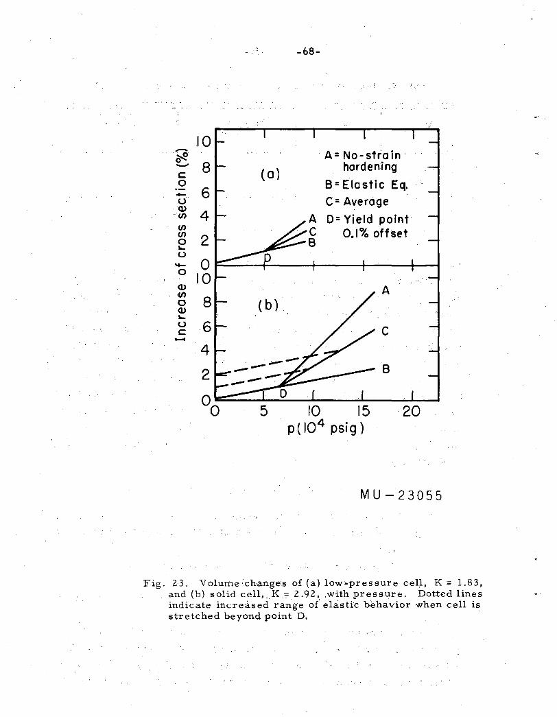
~ -68-

;' '.·

10 -~ A= No-strain · ~ - 8 hardening c (a) 0 B = E I a s tic E q. - 6 u C= Average Q)

-en 4 D= Yield point .en

0.1% offset en 2 0 ~

u '+- 0 0

10 Q) A en 0 8 (b) Q) "-u 6 c c - 4

2 B

00 5 10 15 20 p(I04 psig)

MU-23055

Fig. 23. Volume'.changes of (a) low:..presemre eel~, K = 1.83, and (b) solid cell, .. K = 2.92, .with pressure. Dotted lines indicate increased range o{ elastic behavior when cell is stretched beyond point D.

150,000 psi. This value may be compared to a total cell volume of about 3 cm3.

The compression of the lead washers ( 0.051 em3 total volume) is estimated to be 3 . 0.0012 em ~f one uses the linear coefficient of the compressibility (23.7 x

io-7 per kg/cm2). The thermal contraction of the lead washers relative to

the beryllium copper is oiily 0.0006 cm.3 and can be neglected. If one assumes

that the cross section of the bore increases 5%, then the length of the lead

.washers will decrease 5%, and the volume increase will be 0.0025 cm3. The

stretch of the bore around the front washer should also be about 0.1%.. Hence

the maximum correction for the end plugs at lOjOOO atm should be about 0.5%.

Properties of~ Coseosite ~

The properties of the composite cell may be estimated by considering

that the outer cylinder exerts a pressure on the inner o:ne. Since the outer

one is in the annealed state and is quite close to the yield point, it may be

assumed that the pressure it exerts on the inner cylinder is constant with

respect to stretch of the inner cylinder, The interference fit between the

inner and outer cylinder was designed to be 0.003 in.

The tangential strain at the inner radius of the outer cylinder for

P2 = 0 is given by

(13)

For P1 = 0 the same quantity at the outer radius of the inner cylinder is

The difference between the two strains should·equal 0.003/0.400

Also, P1 equals P2 at the interface. Subtraction gives

( 14)

"'3 = 7o5 X 10 G

Substituting Ki = 2.56 and K; = 2.96, one obtains 34,600 psi as the pressure

on the outside of the inner cylinder. The tangential stress on the inner

radius of the outer cylinder corresponding to the above pressure is given by

... ra ...

= P [~.o + .lJ = 1 2 2.?2 p-1• .. . k - l

0

(15)

= 70,000 psi.

. Since the yield strength of the annealed material is 6o,ooo to ·so,ooo psi,

the inner surface of the outer cylinder _should be at the yield point.

The tangential stress on the inner surface of the inner cylinder at the

limit of elastic behavior is given by

2 p 1 + Ki (P 1 - 2P 2)

K~- 1. C'J = t

Solving for P1 and

~

substituting cr = 130,000 psi, y .

crt (Ki - 1) + 2 P2 K~' 2 .

K. + l J.

= 107,000 psi .•

(16)

we obtain

(17)

· A maximum burst pressure may be calculated by assuming a maximum stress in

the walls of the inner cylinder equal to the ultimate strength (180,000 psi).

This gives

(18a)

P = crt (K. - 1) + P2 K. 1 -~ ~

= 166,000 psi. (18b)

High-Pressure Seals ~ ~ Ce.ll

For the highest pressures, one must use a seal of the unsupported-area

Paul and Warshauer type. The unsupported area-type is preferable, because it

is not necessary to deform part of the cell to. get a seal. However, the use

~··

-7t-

of the unsupported-area principle involves a soft packing which is likely to

have a larger thermal-expansion coefficient than the cell material, so that

maintaining a tight seal down to the lowest temperatures becomes a problem.

Extrusion of' the packing past its supporting parts can also be troublesome.

In the first cell design, a 1/8-in.-thick lead washer was used as the

soft packing. The unsupported area was 0.079 cm2 and the total area 0.34 cm2,

giving_ a packing pressure 3CJfo greater than the pressure in the cell. The front

beryllium-copper washer was 3/16-in. thick and the backing washer was 1/8-in.

thick. The machining tolerances were poorer than 0.001 in. and it was found

that the lead extruded past the backing washer above 50,000 psi. When the

cell was cooled to liquid-nitrogen temperature below 20,000 psi, it leaked

badly.

In the second attempt, the sealing surface was reamed out to 0.281 in.

to get a larger step. The lead washers were made 1/32-in. thick and a 3/64-in.

copper washer was placed on each side of the lead. The copper was dead soft,

and it was hoped that this would prevent the extrusion of' the lead. By using

a thinner lead washer, it was hoped that enough initial compression could be

obtained in the lead and copper washers to compensate for the thermal con­

traction of the lead. A simple calculation indicated that this was a reasonable

expectation. After one compression to 50,000 psi and one cooling cycle, however,

it was not possible to raise the pressure above 32,000 psi because of a large

leak at that pressure. It appeared that the front copper washer spread and

work-hardened, and effectively supported the front beryllium copper washer,

keeping the lead from sealing the gas.

In view of this experience, ·±t was decided to abandon the ·idea of the

copper washers and try to get a close tolerance fit of the beryllium-copper

washers in the bore. Tll;i:s was done in a lathe, and a tolerance of' about

0.0005-in. was achieved. The threaded front washer was still 3/16 in., but

the back one was made 7/16- in. 1 the lead washer still being 1/32 in. When

assembling these par~s it was noticed that the 5-4o threads on the stainless

capillary did not seem to be quite parallel to the axis of the tubing. This

had the effect of putting the two washers at an angle to each ot~r. This

arrangement was found to leak between 30,000 and 4o,ooo psi, but not above or

below. The explanation seemed to be that the front washer was supported by the

bore and could not effectively compress the lead below 4o,ooo psi.· The com­

posite cell was used in this test. The pressure was raised to 94,000 psi,

when failure of' the capillary tubing at a bend halted the test. Evidence for

-72-

extrusion of the lead was still found, although it was not as bad as previously.

The. problem of the 5-40 threads can be solved by usi~g a _guided die-holder, or

by cutting the threads on a lathe. (The. latte! oper~tion. is not convenient

with a long piece of tubing. ) . . 4 . •' It was suggested 5 that the seal could be made good to low temperatures

by backing the lead washer with an annealed gold washer. On ~ooling, the gold

should maintain the initial seal, and the lead would take over at higher

pressures. It is hoped that this approach will make the next test successful.

If it is not possible to ma~intain a leaktight seal during the coo~ing with a

low pressure in the cell, a workable but somewhat inconvenient method would

be to cool the cell under a high pressure of helium, and then put in the

sample under pressure before cooling further.

IV. SAMPLE PREPARATION AND ANALYSIS

Para Hydrogen Converters

Two catalyst chambers::were constructed: one for use with liquid oxygen

or nitrogen, and one for use with liquid hydrogen. Drawings are shown in

Figs •. 24 and 25, respectively. The liquid-nitrogen chamber was placed in a

quart dewar which could be connected to the house vacuum, giving a readily . . 0 ,. ·.

available temperature range of about 60 to 90 K (35 to 57% ortho hydrogen).

The liquid-hydrogen chamber was usually used at the noraml boiling point

(20.4°K) at which the concentra.td,on of ortho hydrogen was e.Z{o. The catalyst used was unsupported ferric hydroxide gel, which has been

found to convert the hydrogen to its equilibrium composition very rapidly~' 47,4B . . - -

It was prep~red by adding·Na0H solution to FeC13

solution and collecting and . . . . . . 0

. washing the precipitate· to remove NaCl. After drying for 24 hr at 85 C and

_for 24 hr at 105°C, the lumps were broken up with a m6rtar and pestle and

particles between No. 30 and No. 50 mesh were collected. About 50 g of catalys~

were put in the liquid-nitrogen cell and evacuated at room t~mperature. After

a day and a half, the pressure over the catalyst had reached 4o ~· It was

then heated to ll0°C. After about 12 hr, the pressure was back to 4o· 1.1 and the

. temperature was raised to 180°C. After 3 hr, the pressure was down to 50 ~, and the vacuum was broken with hydrogen gas and the catalyst was allowed to

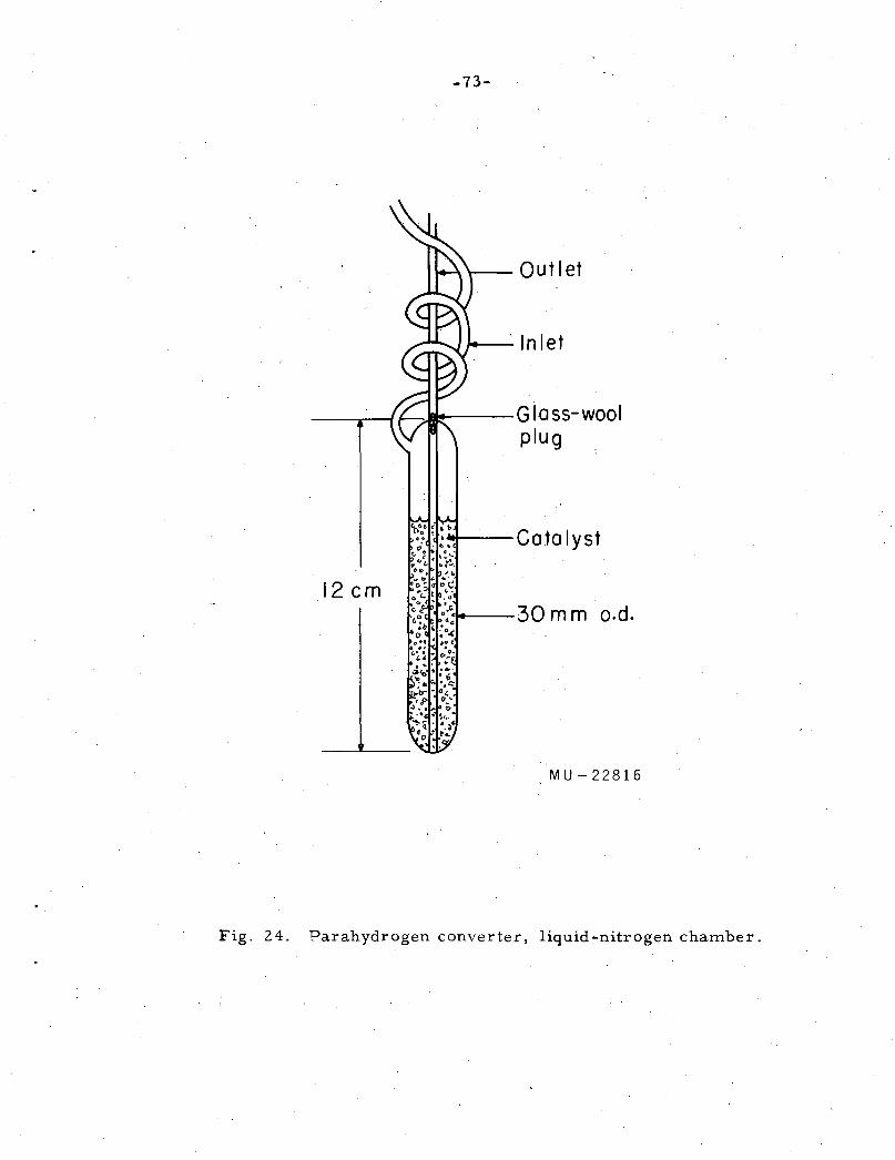
-73-

~-outlet

~-Inlet

---r~ ~---.,.._ ___ G I o ss- woo I plug

12 em ...._-30m m o.d.

MU-22816

Fig. 24. Parahydrogen converter, liquid-nitrogen chamber.

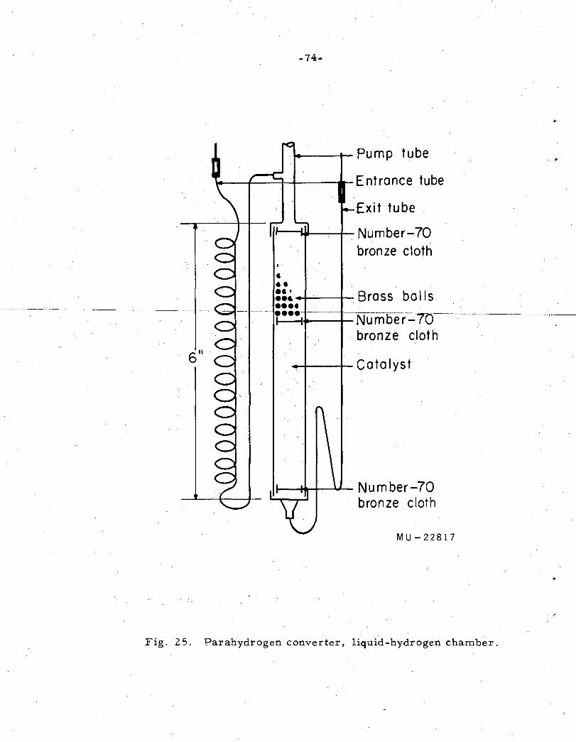
-74-

....... ---+-Pump tube

'-""-+---+--+---.- E nt ranee tube

Exit tube

r--~-......;...f- Number-70 bronze cloth

• •• ::~ 44-"'-----+- Brass b a II s ••••

-·---- ----····---~-J-----1 Number-70--bronze cloth

....... ---t- Catalyst

~.......,.+-......ltwl-- Number-70 bronze cloth

MU-22817

Fig. 25. l?arahydrogen converter, liquid-hydrogen chamber.

•·

·'

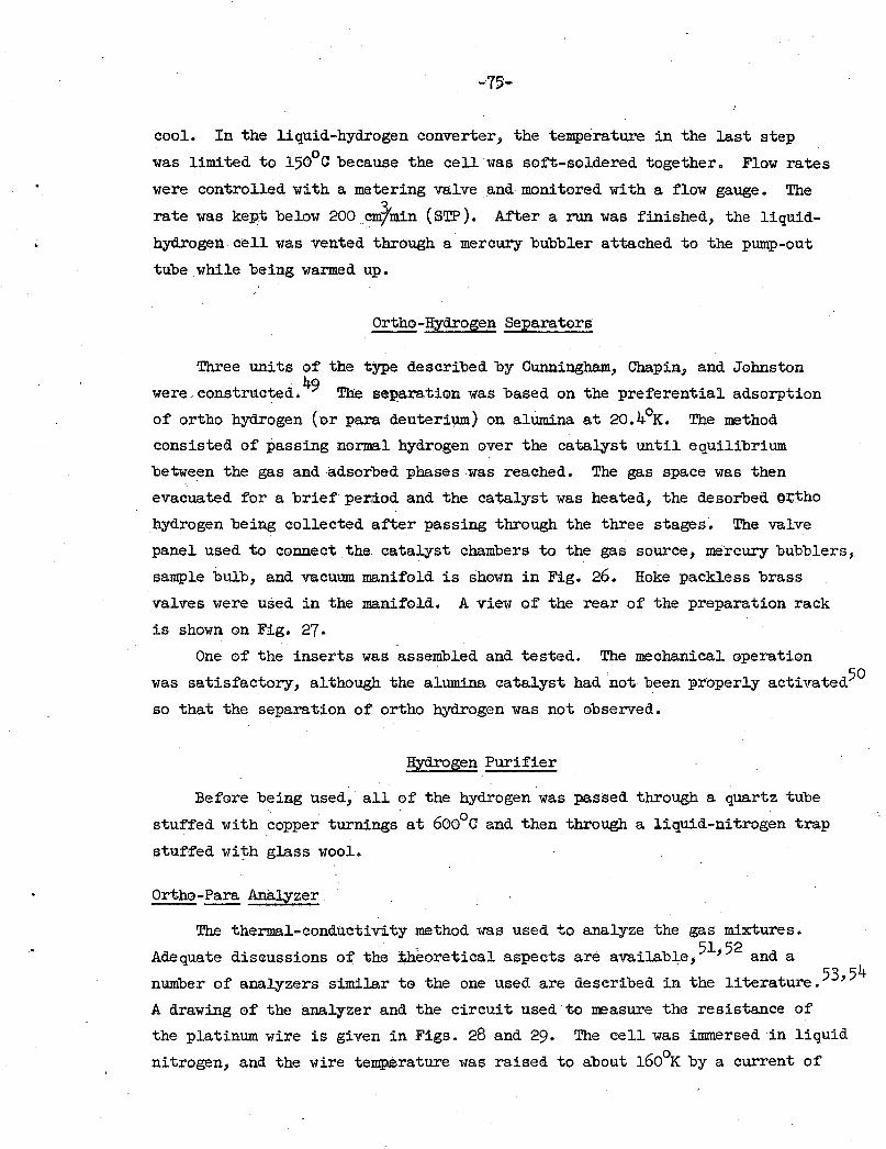
-75-

cool. In the liquid-hydrogen converter, the temperature in the last step

was limited to l50°C because the cell was soft-soldered together. Flow rates

were controlled with a metering valve and monitored with a flow gauge. The

rate was ke:P;t below 200 ,cmfmin (STP ). After a run was finished, the liquid­

hydrogen cell was vented through a mercury bubbler attached to the pump-out

tube while being warmed up.

Ortho-nydrogen Separators

Three units of the type described by Cunningham, Chapin, and Johnston . 49

were,constructed. The separation was based on the preferential adsorption

of ortho hydrogen (or para deuteri~) on alumina at 20.4CJc. The method

consisted of passing normal hydrogen over the catalyst until equilibrium

betwe,en the gas and adsorbed phases was reached. The gas space was then

evacuated for a brief perdod and the catalyst was heated, the desorbed o~tho

hydrogen being collected after passing through the three stages. The valve

panel used to connect the catalyst chambers to the gas source, mercury bubblers,

sample bulb, and vacuum manifold is shown in Fig. 26. Hoke packless brass

valves were used in the manifold. A view of the rear of the preparation rack

is shown on Fig. 27.

One of the inserts was assembled and tested. The mechanical operation

was satisfactory, although the alumina catalyst had 'not been properly activated50

so that the separation of ortho hydrogen was not observed.

Hydrogen Purifier

Before being used, all of the hydrogen was passed through a quartz tube

stuffed with copper turnings at 6oo°C and then through a liquid-nitrogen trap

stuffed wi~h glass wool.

Ortho-Para Ana1yzer

The thermal-conductivity method was used to analyze the gas mixtures.

Adequate discussions of' the Jiheoretical aspects are available, 5l,52 and a

number of analyzers similar to the one used are described in the literature.53, 54

A drawing of the analyzer and the circuit used to me~sure the resistance of

the platinum wire is given in Figs. 28 and 29. The cell was immersed in liquid

nitrogen, and the wire temperature was raised to about 160°K by a current of

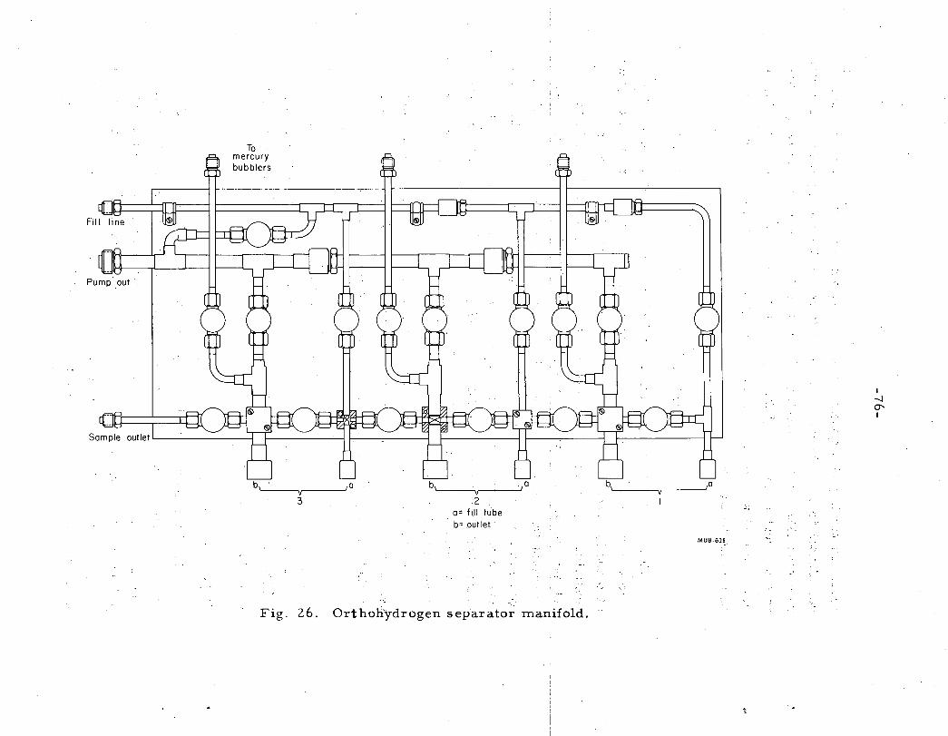
To mercury bubblers

v 3

a= fill tube b= outlet ·

Fig. 26. Orthohydrogen separator manifold.

..;,

MUB-628

~ '·-.:

I -.J 0' I

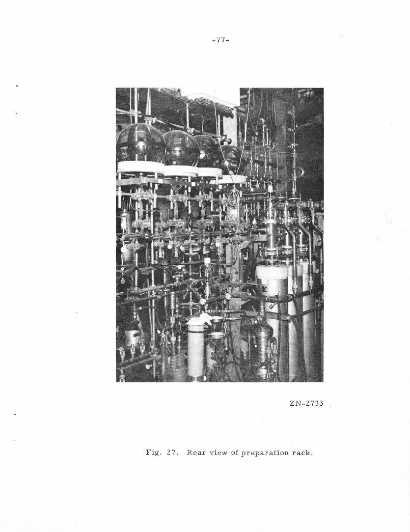
-77-

ZN-2 73 3

Fig. 2 7. Re ar view of preparation rack .

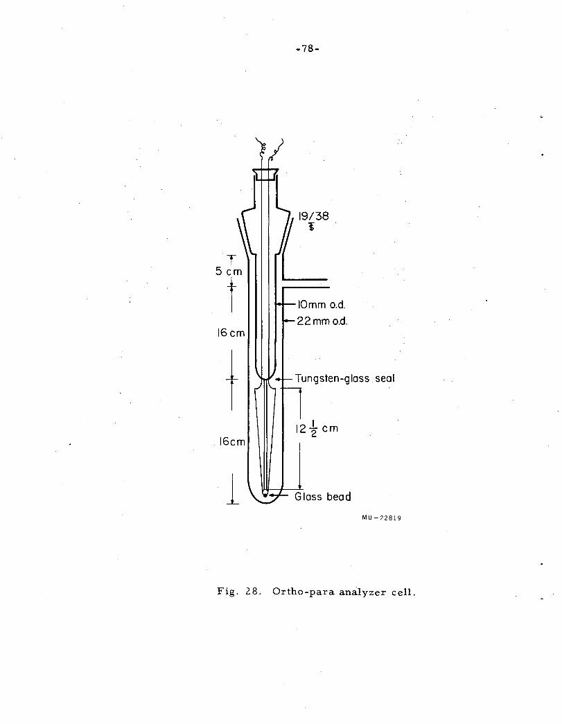
T 5cm

t 16cm

16cm

1

-78-

19/38 1

IOmm o.d.

22mmo.d.

Tungsten-glass. seal

Glass bead

MU-22819

Fig. 28. Ortho-para analyzer cell.

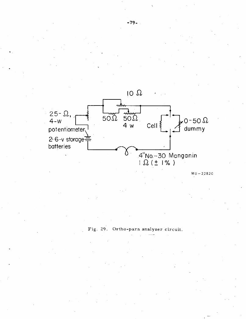
2 5- n, ).----.~-4-w potentiometer.i_

2· 6 -v storage-=­batteries

-79-

IOfl

50fl 50D 4w [

~0-50fl Cell :j dummy

411No.-30 Manganin

lfl(+ 1°/o)

MU-22820

Fig. 29. Ortho-para analyzer circuit.

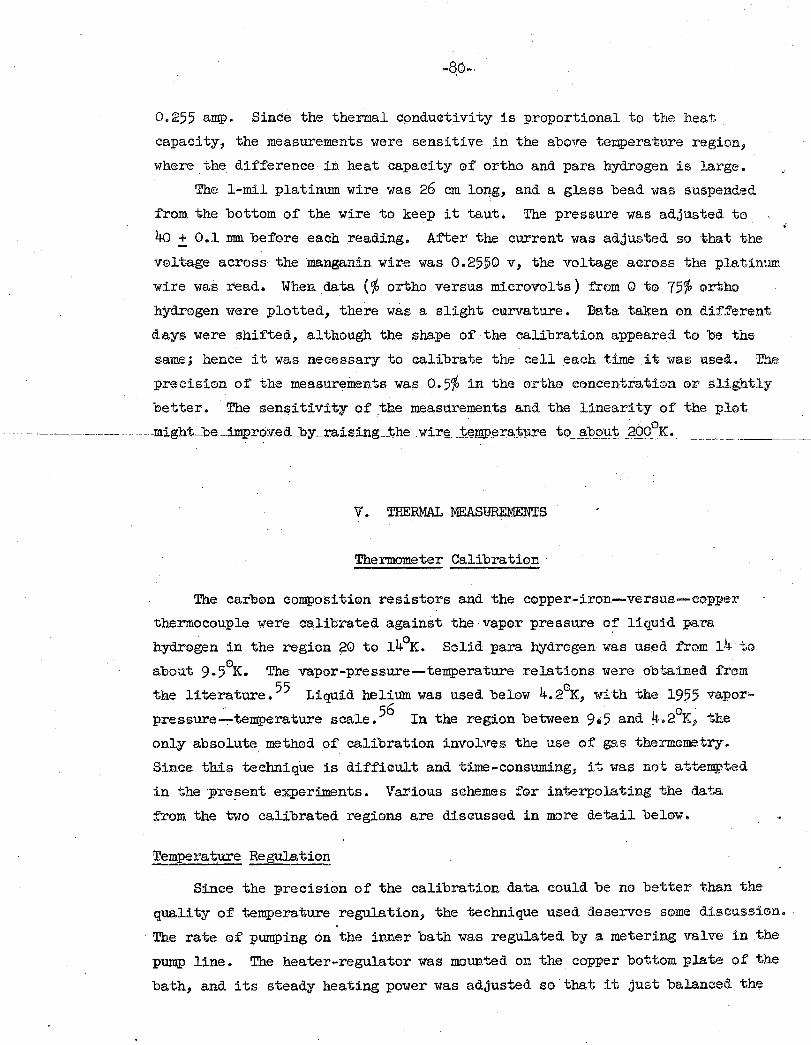
-80-·

0.255 amp. Since the thermal conductivity is proportional to the heat

capacity, the measurements were sensitive .in the above temperature region,

where the difference in heat capacity of ortho and para hydrogen is large.

The 1-mil platinum wire was 26 em lo~g, and a glass bead was suspended

from the bottom of the wire to keep it taut. The pressure was adjusted. to

40 + 0.1 mm before each reading. After the current was adjusted so that the

voltage across the manganin wire was 0.2550 v, the voltage across the platinum

wire was I'ead. When data (% ortho versus microvolts) from 0 to 75% ortho

hydrogen were plotted, there was a slight curvature. Data taken on different

days were shifted, although the shape of the calibration appeared to 'be the

same,; hence it was necessary to calibrate the cell each time it was used. The

precision of the measurements was 0.5'/o in the ortho concentra-tion or slightly

better. ·The sensitivity of the measurements and the linearity of the plot

..

· .. · 0 ~~-~-------~-~-~-----might-be .. impro:v:ed_by_raising_the_~wir.e-.:teJ!lP§:r'~.:l;iJl~~--~.9 __ ~b.9Jl~_?QQ._~·---~-----·------

V. THERMAL MEASUREMENTS

Thermometer Calibration

The carbon composition resiste>rs and the copper-iron-versus-copper

thermocouple were calibrated against the vapor pressure o~ liquid para

hydrogen in the region ~0 to 14°K. Solid para hydrogen was used from 14 to 0 about 9.5 K. The vapor-pressure--temperature relations were obtained from

the literature.55 Liquid helium was used below 4.2°K, with the 1955 vapor~ 56 . 0 .

pressure~temperature scale. In the region between 9e5 and ~·.2 K» the

only absolute method o~ calibration involves the use of gas thermometry.

Since this technique is difficult and time-consuming, it was not a.ttenq;11ted

in ·the ·p:re~ent experiments. Various schemes for interpolating the data

from the two calibrated regions are discussed in more detail bel0W.

Temperature ReguJ_ation

Since the precision of the calibration data could be no better than the

quality of temperature regulation, the technique used deserves some discussion.

T.b.e rate of pumping on the inner bath was regulated by a metering valve in the

pump line. The heater-regulator was mounted on the copper bottom plate of the

bath, and its steady heating power was adjusted so that it just balanced the

-81-

heat loss from the vaporizing liquid. A steady level of about 10 mw was .

fairly common for the bath. With liquid and solid hydrogen and helium I,

there was an appreciable te~erature gradient in the bath because Qf the . ', \

poe:>r heat ccmductivity of the'c.material. However, the thermometer and vapor-

pressure bulbs were all in thermal contact with the copper bottom plate of

the bath, and hence at the same temperature. The most serious difficulty

in connection with the poor thermal conductivity of the bath involved the

establishment of the steady state e . Although it would. have been possible to

set the heater-regulator for a desired temperature, hours we:>uld have been

required to reach a steady state. By heating the bath to approximately the

right temperature, manually holding the temperature constant until a steady

state was set up, and then letting the regulator fUnction, it was possible

to take between one and two readings per hour, depending on the temperature.

Below 12° with solid hydrogen, a gre~ deal of patience was required to reduce

the oscillations of the. temperature of the bottom of the bath sufficiently

to take a set of readings. Above 12°, the establishment of the steady state

was considerably more rapid, and in the liquid-hydrogen region, it was possible

to set up the steady-state temperature in about ten min and complete a set

Of readings in about 1/2 hr. A heating power ef about 1 w was used to raise

the bath temperature from one setting to the next. Liquid helium I appears

to behave like liquid hydrogen, although not much experien.ce has been ' obtained in this region as yet. No points have peen taken in the helium-II

range so far; but the establtiJJ;unent of the steady state should be much easier . '

than in any ef the other regions because of its excellent thermal conductivity.

Procedure for Taking Readings

About 10 min after establishing the steady state, readings were taken of

the vapor pressure, thermometer current and resistance, and thermocouple

potential. The thermome.ter current was read on the K-3 potentiometer and the

potential on the recordere The zero and sensitivity were checked for ~ach

point in the same way as with a galvanometer. Thermometer current and input

to the Rubicon potentiometer were also reversed at each reading to determine

the thermals up to the potentiumetero These were less than 1 ~v, and depended

mainly on the cell temperature. It is reasonable to assume that the origin

of the potential was in the vicinity .of the copper-manga.nin junction at the

shield.

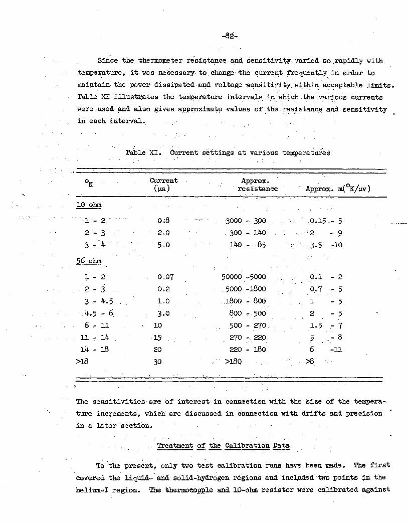
Since the. thermometer resi~tance .ar1d sensitiv:tifY- .varied _so ,rapidly with

tempe~tjll'e, .it was necessary to _change the curre11t ~quentJ.y: in order to

mai:n~in. the power dissipa;ted- a~?-d. voltage -sensi tiy~t.y w~t_hin, acceptable limits~ . .. . . . . . . ·. . . ' ~ . ,•' ..

Table XI illustz:a,tes the t~mperature intervals in. which . th~ various currents . - . .· . .. . '··'" . . - .. . .. were .·used and also gives appi'oximate values of the r~sistanc~ .and sensitivity

in each interval.

Table Xle Current settings at various temperatu.:rks

10 ohm

~- 1'- 2-

2- 3 3 -·4

56 ohm

1- 2 -

~ - 3 3 - 4.5 4.5 - 6 6- 11

11 ~ 14

14 - 18

>18

Current (pa)'

0.;8

2.0

5.0

0.07

0.2

LO

3.0

10

-15

20

30

Approx. resistance

3000 300

300 - 14o

14o - 85

50QOO -5000

5000 -1800

.. 1800 - Boo 800 .,.. 500

500 - 270-

270 - 220

220 - 180

>180

Approx~ m(°K/11v)

.0.1§ -~ 5 ·2 - 9

-3•5 -10

. O.l - 2

0 .• 7 - 5 1 - 5

2 - 5

L5 - 7

5 •. - 8

6 -11

>8

The sensitivities"are of interest-in connection with the size of the tempera­

ture inc:rements, which are discussed in connection with drifts and precision

in a later section.

Treatment~. the Calibration Data

To the pres~nt, oniy two test calibration runs have been made. The first

covered the liquid-- and solid-hydrogen regions and. included'·tWo poin'l;s in the

he1ium-I region. The therm.o.:op.p·le and 10-obm resistor were calibrated ~gainst

..

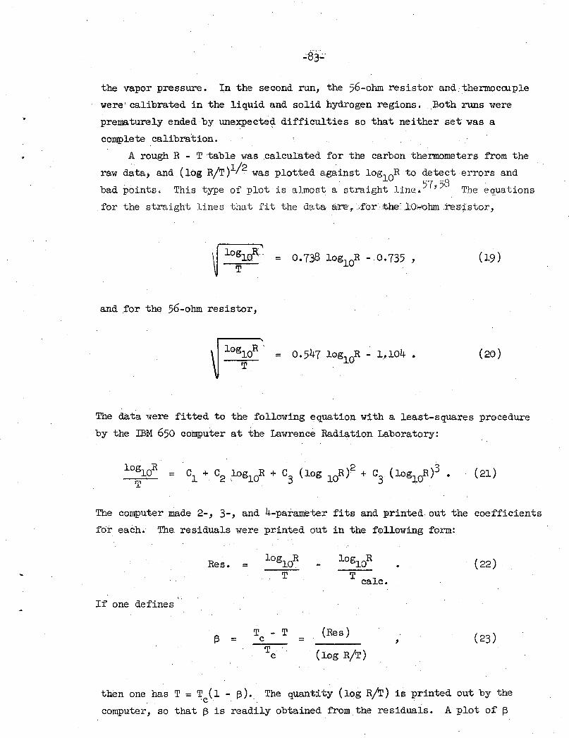
the vapor pressure. In the second run, the 56-ohm resistor and thermoccuple

were' calibrated in the liquid and solid hydrogen regions • .Both runs were

prematurely ended by unexpecte~ difficulties so that neither set was a

complete calibration.

A rough R - T table was calculated for the carbon thermometers from the

raw data, and (log R/T)1/ 2 was plotted against log10R to de~ct errors and

bad points. This type of plot is almost a straight line •57' 58 'I'he equations

for the straight lines that fit the data a:re, ·~for :the ... .lO.,ohm ~s~stor,

~ lo~al'' 0.738 log10R - 0.735 , (19)

and for the 56-ohm resistor,

~ 10g~0R' = 0.547 log10R - 1~104 • (20)

The data were fitted to the following equation with a least-squares procedure

by the IBM 650 computer at the Lawrence Radiation Laboratory:

(21)

The computer made 2-, 3-, and 4-parameter fits and printed. out the coefficients

for each. The residuals were printed out in the f0llowing form:

R log

10R

es. = (22) T

If one defines

T - T (Res) c = ' (23)

Tc (log R/T)

then one has T = T/1 - t3) •. The quantity (log R/T) is printed out by the

computer, so that t3 is readily obtained from the residuals. A plot of t3

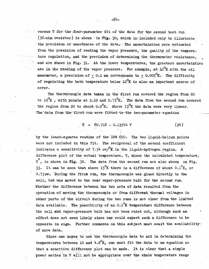
.. a:4-·

versus T for::the' ,four-parameter fit·. of the data for the -second test run • • • ' - • u -· ' • ' .,

( 56-ohnl. resistor) is:: shown .: in Fig.- ·30, ~Which in· included only ,to :illustrate

the ·precision or:;smoothness of'. the data.· >The uncertainties· were estimated . . . -. . ' -" ... : .

from the pre.cision of reading the vapor pres.sure, the quality~of the tempera­

ture regu.J.ation, and the precision of' determining the thermometer resistance, ~·

'and are shownin Fig~ -31. At the lower temperatures, the,greatest uncertainties

are in the :reading of'. the vapor pressure. For example,.· at ·lOCX:.with the oil

manometer, a precision of'.:!: O~l mm corre.sponds ·to .:!: Oo005°K.- The difficulty

of' regulating the bath temperature below 12°K is also an important source of'

error.

The the:ctn6couple data taken in the.first run covered the region from 20

to 12°K , with points at 3.19 and 2. 73°K.' The data from the second run covered 0 0 the region from 20 to about 9.,2 Ko Above 13 K the data were very linear.

The-da.ta-f'rom-the-·f'irst-run ·were--fitted-to--the-- two~parameter -eq~tion

T = 80.718 - 0.13544 V (~4)

by the least-squares routine of the IBM 650. The two liquid-heliUm points

were not included in this fit. The reciprocal of the second coefficient

indic~tes a sensitivity of' 7.34 JJ.vfK.in the liquid-hydrogen re,gion~ A

difference plot of the actual temperature, T, minus the calculated temperature, * . ' . ' . T , is shown in Fig. 32. The data from the second run are also shown on Fig.

33. It can be seen that above 13°K there is ~ differenc~ of about O.l°K, or

0. 7311V'·· During ·the first> run, the thermocouple was glued directly to the

cell, but was moved to the rear vapor-pressure bulb for the second run •

.. Whether. the difference between the two .sets of data resulted from the

operation of moving the thermocouple or fro~ different;· thermal voltages in

o:ther parts of the circuit during the two runs is not clear from the limited

data available. The ·:possibility· of an O.l°K temperature difference between

the cell and vapor~pressure bulb has not been ruled out, although such an

effect does not seem likely since one would expect such ~ difference to be

opposite in sign. Further comments on this subject must await the availability·

of more data.

Since one hope~.to use the the:r:iri0couple data to aid in determining the . . . 0

temperatures between 10 and 4.2 K, one must fit the data to an equation so

that a sensitive.di:~erence plot can be made •. It is clear that a simple

power series '·in "v will not be ·appropriate over the whole temperature range • ~ • 1 :... ! ·' • • • J • '

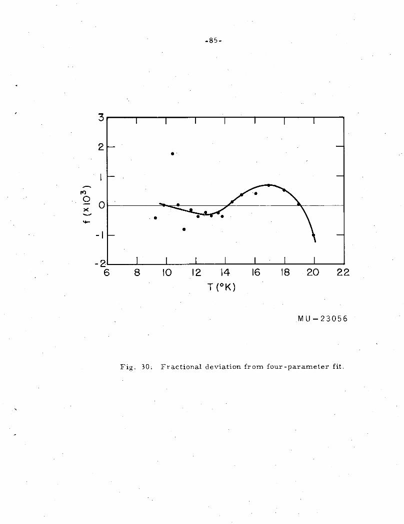
-85-

2 •

-rt)

0 0 )( ......,

• ......

- I

-2~----~--------~----~--------~----~--------~--------~----~ 6 8 10 16 18 20 22

MU-23056

Fig. 30. Fractional deviation from four-parameter fit.

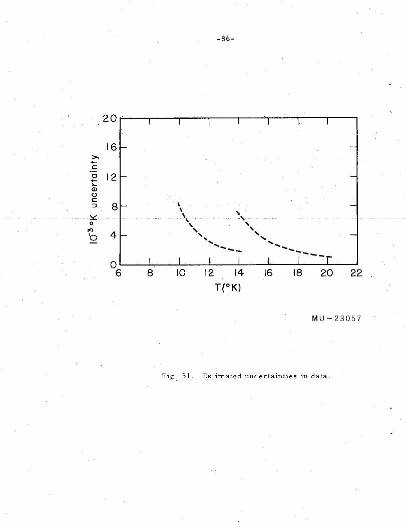
16 ~ -c ·-c 12 -!h.. Q)

0 c :::J 8

~-~-------- ---- --~----------~-C- ---- .. -• --

0 rt)

'o 4

-86-

o~~~~--~--~----~~~~--~----~--~

6 8 10 12 14 16 18 20 22 '

T(°K)

MU-23057

Fig. 31. Estimated uncertainties in data.

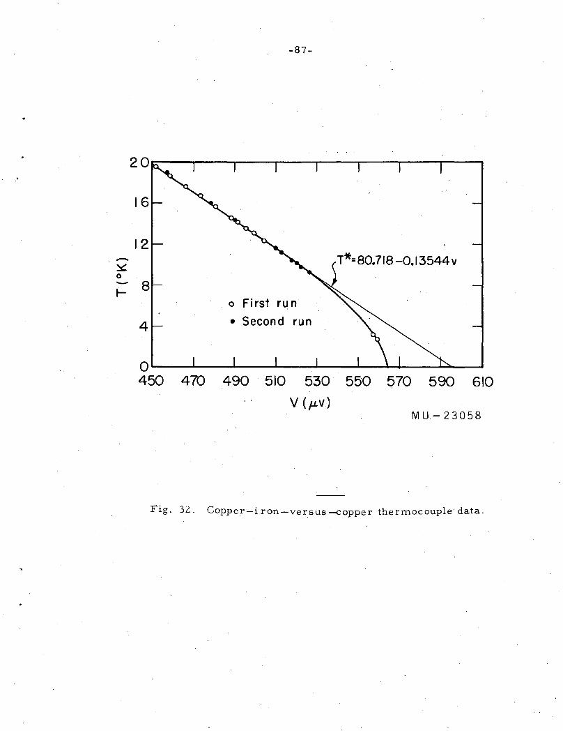
-87-

16

12 - T*=80.718 -0.13544v

-o First run

4 • Second run

o~--~--~----~--~--~--~~--_.._~

450 470 490 510 530 550 570 590 610

V(J-LV) MU-23058

Fig. 32. Copper-i ron-ver,sus -copper thermocouple data.

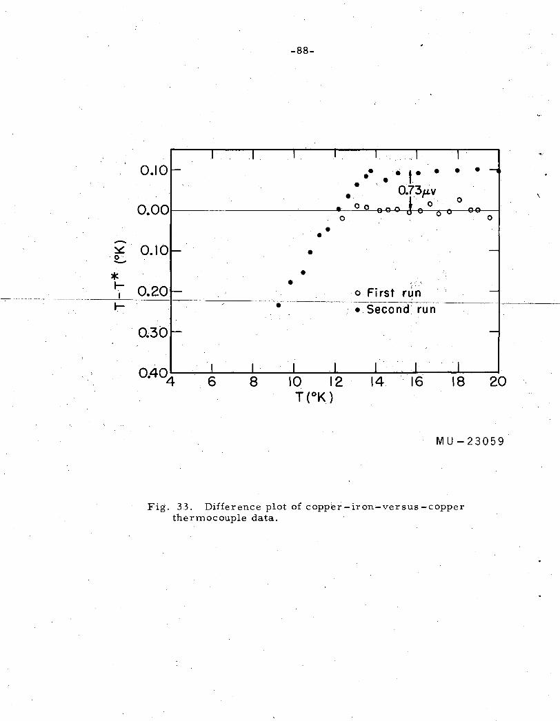
-~ ·o -* ~

I

I-

-88-

0.10 • • t• • • • • • • 0.73p_v

0.00 0 0

• • •

• • ·'. ".

First ; ...

0 run ;

• • Second· run

0.30

20

MU-23059

Fig. 33. Difference plot of copper-iron--versus -copper thermocouple data.

···;

\

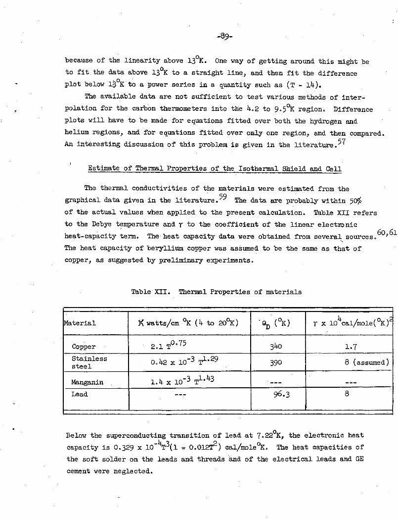
because of the linearity above 13°K. One way of getting around this might be . 0

to fit the data above 13 K to a straight line, and then fit the difference

plot below 13°K t~ a power series in a quantity such as (T - 14).

The available data are not sufficient to test various methods of inter­

polation for the carbon thermometers into the 4.2 to 9.5°K region. Difference

plots will have to be made for equations fitted over both the hydrogen and

helium regions, and for equations fitted over only one region, and then compared.

An interesting discussion of this problem is given in the literature.57

Estimate of Thermal Properties of the Isothermal Shield and Cell

The thermal conductivities of the materials were estimated from the

graphical data given in the literature. 59 The data are probably within 5o%

of the actual values when applied to the present calculation. Table XII refers

to the Debye temperature and r to the coefficient of the linear electiOnic

heat-capacity ~rm. The heat capacity data were obtained from several sources. 60>61

,_

The heat capacity of beryllium copper was assumed to _be the same as that of

copper, as suggested by preliminary experiments.

Table XII. Thermal Properties of materials

!Material ){watts/em °K ( 4 to 20°K) . Q (OK) D y X l04cal/mole(°K)2

Copper 2.1 T0 .. 75 340 1.7

Stainless 0.42 X 10~3 T1•29 390 8 (assumed) steel

Manganin 1.4 X 10-3 T1 •43 --- ---Lead --- 96.3 8

Below the superconducting transition of lead at 7.22°K, the electronic heat

capacity is 0.329 x l0-4T3(1 = 0.012~) cal/mole°K. The heat capacities of

the soft solder on the leads and threads and of the electrical leads and GE

cement were neglected.

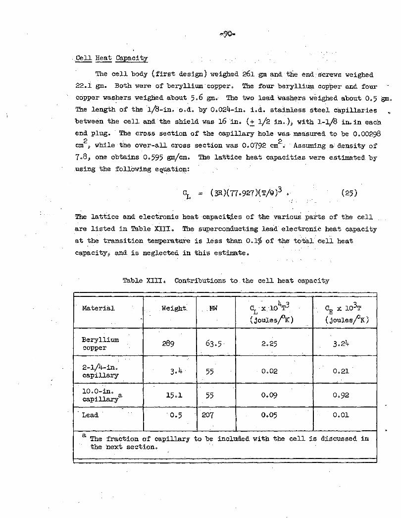
.Cell Heat Capacity

The cell body (first design) weighed 261 gm. and the end.· screws weighed

22. l gm.. Both were of beryllium· copper., · The four beryllluln. copper and four

copper washers weighed about 5.6 gm.. The two lead washers weighed about 0.5 gm.

The length of the ·1/8-in. o.d. by 0.024-in. i.d. stainless steel capillaries •

between the cell and the shield was 16 in~ (.±. l/2 in., h with l-1/8 in. in each

end plug. · The cross section of the capillary hole was. measured to be 0.00298

cm2

» while the over-all cross section was 0.0792 cm2 • Assuming a: density of

7 .8:~ one obtains 0.595 f!lJl/cm. The latt.ice heat capacities were estimated by

using the following eq~tiop.:

(25)

The lattice and electronic heat capacit;tes of' the various parts of the cell

are listed in Table .XIIIo .The superconducting lead electronic heat capacity

at the transition temperature is less than 0.1~ of the total cell heat

capacity; and is neglected in this estimate.

Table Xni., ContribUtions to. the cell heat capacity

. c 4 ~ X 103T Material . Weight. MW" ~ x·lo T3

.. . ( joulesfK) ~joulesfK)

Beryllium 289 63·5 2.25 3.24 copper

'.

2-1/4-in. 3 .. 4. 55 0.02 0.21 capillary

10.0-in. ..

capillar.l l5ol 55 0.09 0.92

-Lead

.. 0.5 207 0.05 0.01

a The fraction of capillary to be included with the cell is d.iscussed in the next section.

.•.

•.

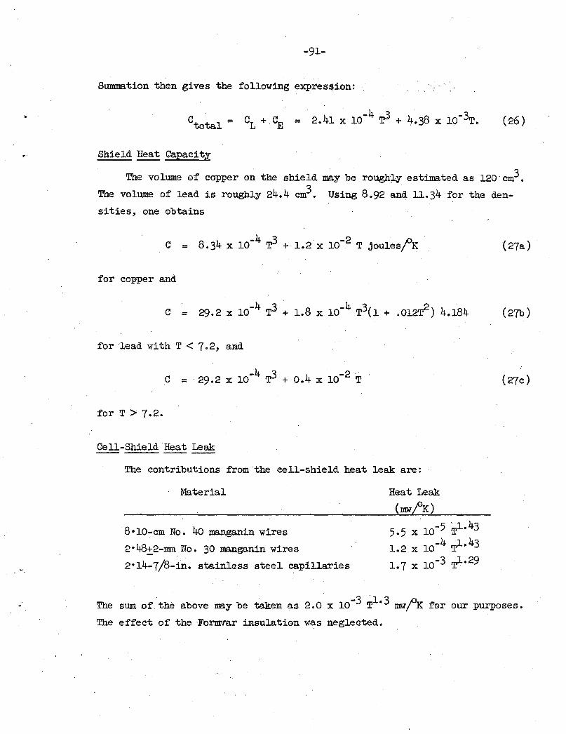
-91-

Summation then gives the following expression:

4 -4 3 4 8 -3 Ct t l = CL + CE = 2. 1 x 10 T + .•3 x 10 T. o a

Shield ~ Capacity

(26)

The volume of copper on the shield may be rough;Ly estimated as 120 cm3.

The volume of lead is roughly 24.4 cm3. Using 8.92 and 11.34 for the den­

sities, one obtains

for copper and

for 'lead with T < 7.2, and

-4 3 4 -2 . C = 29.2 X 10 T + 0. X 10 T

for T > 7.2.

Cell-Shield Heat Leak

The contributions from the cell-shield heat leak are:

Material

8•10-cm No. 4o manganin wires

2·48~2-mm No. 30 ma.nganin wires

2•14-7/8-in. stainless steel capillaries

Heat Leak

(mwfK)

5·5 X lo-5 Tl. 43

1.2 X 10-4 ~· 43

l. 7 X 10-3 Tl. 29

(27a)

(27b)

(27c)

The sum of the above may be taken as 2.0 x 10-3 Tl. 3 mwj>K for our purposes.

The effect of the Formvar insulation was neglected.

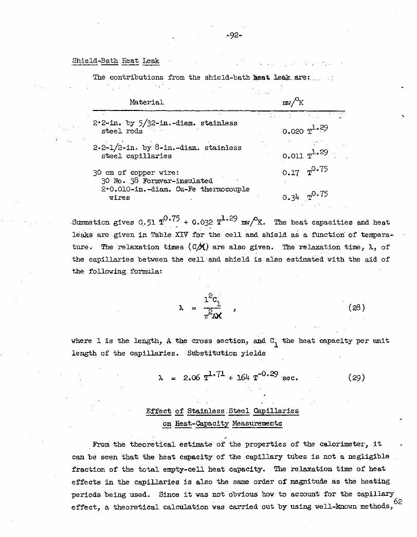
Shield-Bath Heat Leak

The contributions from the shield-bath beat. .. leak are_:_

Material

2•2-in. by 5/32-in.-diam. stainless steel rods · ·. ·

2·2·1/2~in, by 8-in~·diam. stainless steel capillaries

30 cm_of copper wire: 30 No. 38 Formvar-:i.nsulated. 2•0.010-in. -diam. Cu-Fe thermocouple

wires

0.011 TL 29 ·

0.17 T0 •75

-SUlmllation gives 0. 51 T~".7? + 0.03~ r" 29 rrMfK. The heat capacities and heat

leaks are given in Table XIV for the cell and shield as a function of tempera.-.·

ture. The relaxation times (C,b{) are also given. The relaxation time, 1t., of

the capillaries between the cell and shield is also estimated with the aid of

the following formula:

(28)

where 1 is the length, A the cross section, and c1

the heat capacity per unit

length of the capillaries. Substitution yields

Effect of Stainless.Steel Capillaries

~ ~-Capacity Measurements

/

(29)

From the theoretical estimate o:f' the properties of the calorimeter, it

can be seen that the heat capacity of the capillary tubes is not a negligible

fraction of the total empty-cell heat capacity. The relaxation time of heat

effects in the capillaries is also the same order of magnitude as the heating

periods being used. Since it was not obvious how to account for the capillary 62

effect, a theoretical calculation was carried out by using well ... known methods,

•· ..

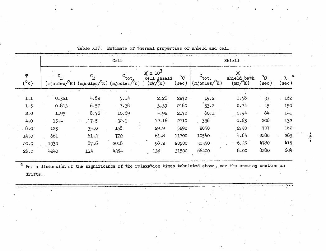
Table XIV. Estimate of thermal properties of shield and cell

Gell I Shield ~~-- ------ .. ------ --- -~~-~ --~-~-· -·--·- ..

T I ct · cE ctot. )(X 103

"'c c )'( Ts a cell shield tot. shield bath )..

(OK) (mjoules;oK) (mjoules;oK) (mjoulesj°K) (~/'K) (sec) (mjoules;oK) (mw;oK) (sec) (sec)

1.1 0.321 4.82 5.14 2.26 2270 19.2 0.58 33 162

1.5 0.813 6.57 7.38 . 3·39 2180 33.2 0.74 45 150 2.0 1.93 8.76 10.69 4.92 2170 60.1 .. 0.94 64 141

4.0 15.4 17.5 32-9 12.16 2710 336 1.63 206 132

8.0 1.23 35.0 -158- 29.9 5290 2050 2.90 707 162

14.0 661 61.3 7g2 61.8 11700 10540 4.64 . 2280 263 I '!) VJ

20.0 1930 87.6 2018 98 .. 2 20500 30350 6.35 4780 415 I

26.0 424o 114 4354 138 31500 66400. 8.00 8280 604

a For a discussion of the significance of the relaxation times tabulated above, see the ensuing section on

drifts •.

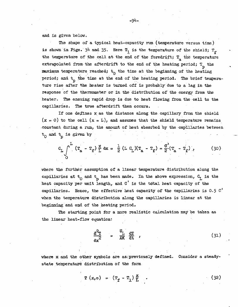
and is given below.

The shape of a typical heat-capacity run (temperature versus time)

is shown in Figs. 34 and 35. Here T1 is the temperature of' the shield; T:f'

the temperature o,f the cell at the end of' the foredr:i,f't; Ta the temperature

extrapolated from the a:f'terdrift to the end of the heating period; T the . p

maximum temperature. reached; t 0 the time at the beginning of the heating \'. . . .

period; and tp ~he time at the end of the heating period. The brief tempera~

ture rise after the beater is turned off is probably due to a lag in the . response of' the thermometer or in the ·distribution of the energy from the

heater. The ensuing rapid drop is due to heat flowing from the cell to the

capillaries. The true afterdrif't then occurs.

If one de,fines x as the distance along the capillary from the shield

(x = 0) to the cell (x = L), and assumes that the shield temperature remains

constant during a run, the amount of heat absorbed by the capillaries between

t 0 and t is given by p.

L 1 cr' CL J (~a - Tf) I dx = 2 (L CL)(Ta .. Tf) = 2(Ta - Tf) 3 (30)

0

where the furtb.Sr assumption of a linear temperature distribution along the

capillaries at t0

and tp has been made. In the above expression; CL is the

heat capacity per unit length, and C' is the total heat capacity of the

capillaries. Hence, the effective heat capacity of the capillaries is 0.5 c' when the temperature distribution along the capillaries is linear at the

beginnin$ and end of the heating periodo

The starting point for a more realistic calculation may be taken as

the linear heat-flow equation:

= (31)

where x and the other s:ymbols are as~:previously defined. Consider a steady­

state . tein;perature distribution of' the form

(32)

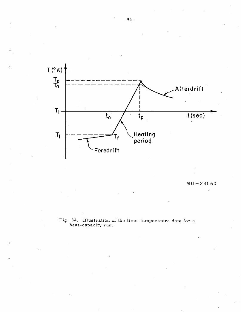
-9 5-

-----· ------- ...

Foredrift

Heating period

Afterd rift

MU-23060

Fig. 34. Illustration of the time-temperature data for a heat-capacity run.

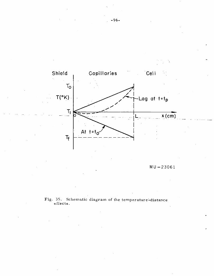
-96-

Shield Capillaries Cell

at t=tp

At

MU-23061

Fig. 35. Schematic diagram of the teinperature:..distance effects.

-97-

If the value of Tf is increased 1°K at t = 0 and then held constant, the new

steady state will be

·( ) ( ) X ·X T x, co = Tf - Tl L + L .·· . '

and the solution at arbitrary times is found to be

2 co + - z

7f n=l

(33)

(34)

The part of the temperature distribution resulting from the unit temperature

rise is given by A(x,t), which is defined by

2 ~ (-l)n . nnx -n2tjl = ! + - X - s~n - e ( 35 )

L 7f n=l n L

If a series of temperature rises F(O), F(-r1 ) - F(O), F(-r2 )- F(-r1 ), ••• take

place at times o, T1

, T2, ••• , at x = L, the linearity of the problem may be

utilized to obtain the temperature distribution at the instant following

t = T as follows: n

(36)

+ [F(-r)- F(-r 1)] A(x,t- T), n n- n

where

(37)

If one writes

Eq. (36) may be written

T1(x,t) = F(O) A(x,t) + ~ A(x,t--rk) (::_! bt"k •

. . . k=l .

By allowing the number of jumps to become infinite while the jumps and

intervals tend to zero, one obtains the following limiting form:

Jt

.. T'(x,t) = F(O)cA(x,t) + _ A(x,t--r) F\<r)d-r • _ ·-0

For the duration of the heating period (taking t0

as o), one may assume

Combination of Eqs. (35), (4o), and (41) gives

T-T[ oo ( )'n 2A ] T'(x,t) = p t f r t + ~ z-~ (1-e-n t,A, sin n~ '

~ p · D:=l n

(38)

(39)

( 4o)

(41)

(42)

from which one obtains the temperature distribution in the capillaries up to t ! p

(T -Tf) · ~ ( )n 2 A T(x,t) = (T"' .. T

1) _Lx + pt ! t + 2rr Z -l (l-e-n t/"')sin mrx. ( 43) •

• L A n-l 3 L · P - n .

The temperature distribution after tp is considered in a later paragraph.

~.

-99-

The heat flow from the cell to the capillaries during the heating

period is given by

and the heat flow from the capillaries to the block is

( 44)'

(45)

The total heats flowing from the cell to the capillary and from the capillary

to the block are ·

H Jtp AX. .(d~)_ dt +1ts .A)( (dT.) dt 1. = dx)x-L t dx)x=L

0 p

(46)

and

H2 =· ltp AX (.d~\_ . dt + lts AX. (d~) dt ' 0 ~~ t ~~

(47) ' p

where t is sufficiently greater than t that the steady"state drift has been s p established. The difference between Eqs. ( 46) and ( 47) represents the heat

that goes to change the temperature of the capillaries. The first term of

Eq. (47) represents the heat flow from the cell and capillaries to the environ­

ment during the heating period, and the second term represents the flow after

the heating period.

At this point it becomes apparent that one of two approaches may be

followed in order to treat the effect of the capillaries on the heat-capacity

measurement:

a. The capillaries may be considered as part of _the environment. The

correction in this case would consist of calculating Eqo (46) and subtracting

it from the heat input in order to obtain only the heat capacity of the cell

and contents.

b. The capillaries may be considered as part of the cell. The

correction to the heat input in this case involves only the amount of heat

that passes from the capillaries to the environment during the heating

period and during the time necessary to attain the steady state in the

-100-

I·

capillaries.

Since most of the heat absorbed by the capillaries comes from the cell, the

second approach is the more reasonable, because it should involve the smallest·

calculated correction.

The calculation is carried out as follows: The first term of Eq. (47) is 4

evaluated to give the heat flow from the capillaries to the environment during

the heating period. The second term is evaluated by making the approximation

that the cell temperature relna.insat a constant temperature (Ta) while the

capillaries relax to the linear temperature distribution: T = T1 + (Ta - T1 )xjL.

The difference between the heat that would flow from the capillaries to the

environment if the steady state had already been reached, and the amount that

actually flows, gives the correction.

The appropriate derivative during the heating period is

( 48)

and the integral is

(49)

For ~q. ( 49) to be use:NJ.., the block temperature must be eliminated since

it is not readily determined during an experiment. Since the fore and after

drifts are easily determined, one may write

dTf 1: (T - T ) dt = T 1 f

(50) dT

1: (T - ~ ) J = dt T 1 p . , where

T LC

= XA (51)

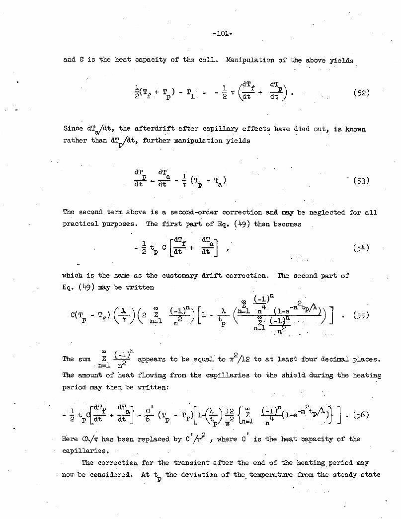
-101-

and C is the heat capacity of the cell. Manipulation of the above yields

(52)

Since dTa/dt, the afterdri~t after capillary effects have died out, is known

rather than dTpidt, further manipulation yields

dT dT 1 _R = ~ - - (T - T ) dt dt T p a (53)

The second term above is a second-order correction and may be neglected for all

practical purposes. The first part of Eq. (49) then becomes

which is the same as the customary drift correction.

Eq. (49) may be written

C( T .. T ) c· ;N) (2 i p f T n=l

(54)

The second part of

(55)

oo ( l)n 2 . . The sum i: -T appears to be equal to 7r /12 to at least four decimal places.

· n=l n The amount of heat flowing from the capillaries to the shield during the heating

period may then be written:

- 1: t c[dT:f.' + dTaJ- i (T .. T )[1-(~)· 12 f Z ( .. t)n(l•e.-n~i>p/A.)l J • (56) 2 p dt dt o p f tp 71:2 ln=l n . 'J

' 2 ' Here C>../r has been .replaced by C /v , where C is the heat capacity of the

capillaries.

The correction for the transient after the end of the heating period may

now be considered. At t the deviation of the temperature from the steady state p . .. ..

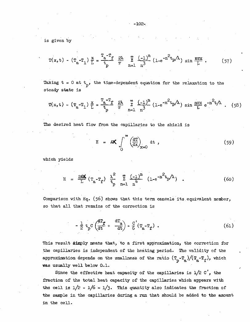
-·102-:

is given by

T -Tf 2l T(x,t) - (T •T ) ~ =_a_

a 1 L t 1r (57) p

Taking t = 0 at t , the time-dependent equation for the relaxation to the . p steady state is

The desired heat flow from the capillaries to the shield is

00

H = PX. 1 r:) dt , O ~ X=O

which yields

Z (-U)n (l-e-n2tp/A) n=l n

(59)

(60)

Comparison with Eq. (56) shows that this term cancels its equivalent member,

so that all that remains of the correction is

(61)

This result simply means that, to a first approximation, the correction for

the capillaries is independent of the heating period. The validity of the

approximation depends on the smallness of the ratio (T -T )/(T -Tf), which p a a

was usually well below 0.1.

Since the effective heat capacity of the capillaries is 1/2 c', the

fraction of the total heat capacity of the capillaries which appears with

the cell is 1/2 - 1/6 ·= 1/3· This quantity also indicates the fraction of

the sample in the capillaries during a run that should be added to the amount

in the cell.

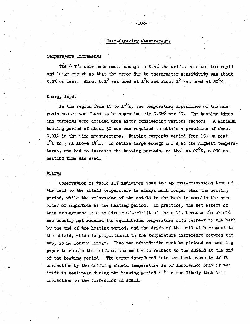
-103-

Heat-Capacity Measurements

Temperature Increments

The b. T 's were made small enough so that the drifts were not too rapid

and large enough so that the error due to thermometer sensitivity was about

0.2$ or less. About 0.1° was used at 1°K and about 1° was used at 20°K.

Energy Input

In the region from 10 to 17°K, the temperature dependence of the man­

g.anin heater was found to be approximately 0.06% per °K. The heating times

and currents were decided upon after considering various factors. A minimum

·heating period of about 30 sec was required to obtain a precision of about

0.01% in the time measurements. Heating currents varied from 150 1J.8. near

1 °K to 3 ~ above 14°K. To obtain large enough b. T 's at the highest tempera­

tures, one had to increase the heating periods, so that at 20°K, a 200-sec

heating time was used.

Drifts

Observation of Table XIV indicates that the thermal-relaxation time of

the cell to the shield temperature is always much longer than the heating

period, while the relaxation of the shield to the bath is usually the same

order of magnitude as the heating period. In practice, the net effect of

this arrangement. is a nonlinear afterdrif't of the cell, because the shield

has usually not reached its equilibrium temperature with respect to the bath

by the end of the heating period, and the drift of the cell with respect to

the shield, which is proportional to the temperature difference between the

two, is no longer linear. Thus the afterdrifts must .be plotted on semi-log

paper to obtain the drift of the ce:ll with respect to the shield at the end

of the heating period. The error introduced into t~e heat-capacity drift

correction by the drifting shield temperature is of importance only if the

drift is nonlinear during the heating period. It seems likely that this

correction to the correction is small.

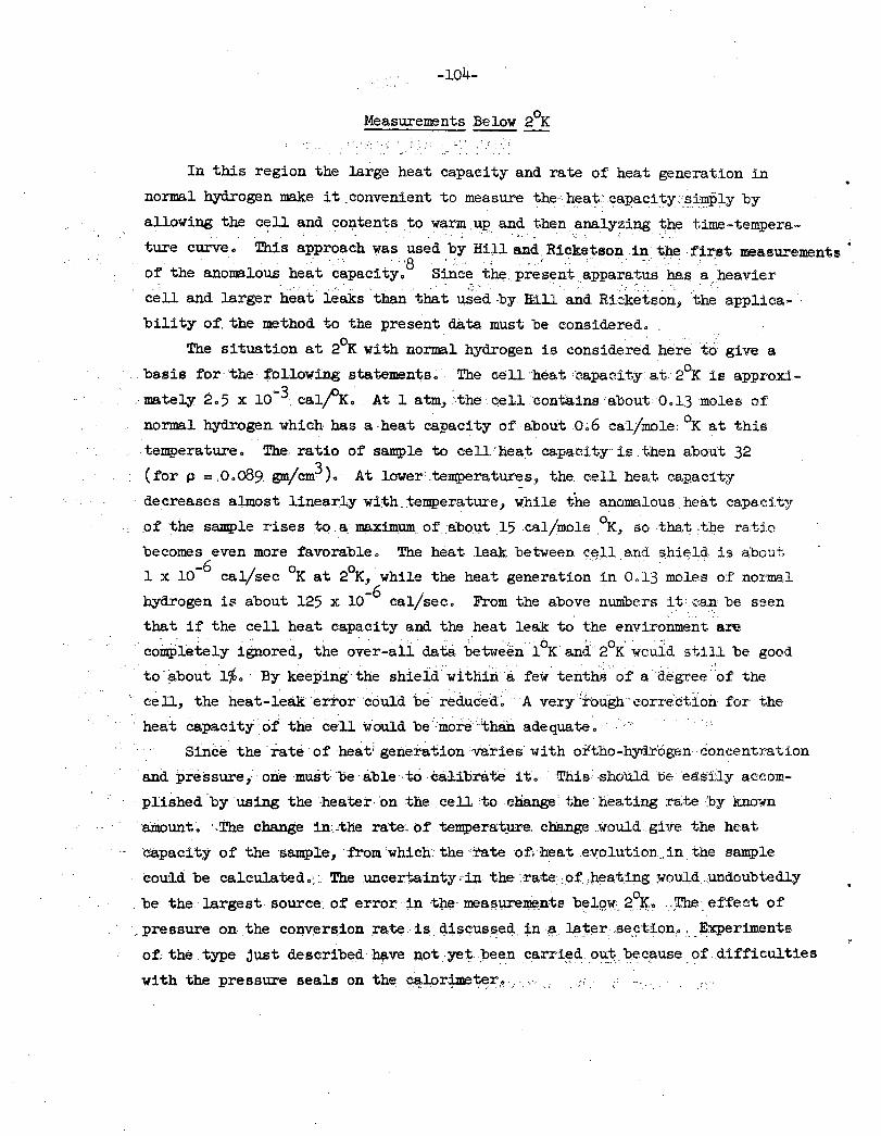
-104-

0 Measurements Below 2 K

In this region the large heat capacity and rate of heat generation in

normal hydrogen make it_convenient to measure the·heat:ca:f:lacity:c_~iJnply by

allowing the _cell and coQ.tents to warm up and then analyzing the time-tempera-• • • • •• • • ~ •• •• - •• ' ¥ • • ; • • • • : •

ture curve. This approach was used by Hill and. Ricketson in the first measurements · - . ·., .. ··a . , : . . .. . . . . . .. : of the anomalous heat capacity. Sine~ the present_appara~us has .aheavier

cell and larger heat i~aks 'than that u~~d -by llill and RicketsonJ the applica-.

bility of. the ~thod to the present data must be considered •. 0 . ' . . ....

The situation at 2 K with normal hydrogen is considered here to give a

basis for the following statements. The cell·heat ·capacity at 2°K is approxi-

. mately 2.5 x 10-3 ca.l/'K. At l atm, :the·. cell contains ·about: 0.1.3 moles of

normal hydrogen which has a heat capacity of -about 0~6 cal/mole•. °K at this

temperature. The· ratio .of sample to cell-'heat capacity· is then about 32

(for p = .O.o89 gmfcm3 ). At lower: temperatures, the cell. heat capacity

· de creases almoSt linearly wlth, temperature, while the anomalous . heat capac:i ty

.of the sample rises to a~ maximum_ of abo;q.t 15 cal/mole °K, so that :i:il:le ratj.o

becomes even more favorable. The heat leak between e;::~,ll and shiS:ld is about -6 , 1 o o l x 10 ca~sec Kat 2 K, while the heat generation in 0.13 moles of nor~l.

-6 I hydrogen i~ about 125 x 10 cal sec. From the above nunibers it·- can be seen ...

that if the cell heat capacity and the heat leak to the environment are .· . . .. .· . . . . . '·. .. . .... -.. . b ·'· 0 . . ·;

coin:.Pletely ignored, the over-all data between 1 K and 2 K would still be good

to- i:tbout l'{o. By keeping'· the shield wi thfu a few tenths of a ilegr.ee 'of the

cell, the heat-l~ak error ·could be reduced~ A very :rough· correction for the

· heat capacity' of the ce:ll would be -more thB.D. adequate.

Since the·rate·of: heat; generationv'arieswith ortho-b.ydr'ogenconc:entration

-·and pressure,- one mu8t: be able -to calibrate it. This: -shoUld ·be eas:l:l.y accom­

plished-by using the -heater. on the cell to cbangetheheating ra:te:by kno-wn

· 'aJilOunt~ ·.The change in: .. the rate·. of temperat_ure, change would. give the heat

da.pacity of the sample, from which. the ·rate of'; heat .eyolution .. in the sample

coufl.d be calculated.;:. The uncertainty :·in the :rate ,of )lea'ting :would ,Jmdoubtedly

. be the ·largest ·source ot error· in ·tlle· mea~ure~nts b~lgw_ 2°1{:.. . ,_The·. effect of

· .. pressure on . the converdon rate. is. q.isCUSf!ed.-. in .a la~er .se_ction:• , __ ]:xperiments

of: the type just described ~ve not.ye~ been ca:rri~d _out.l?~~use of difficulties

with the pressure seals on the Cf!.lor.imeter. , .. , . . . -.. ···- ..

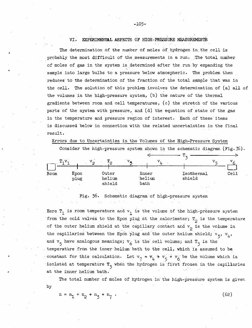
VI. EXPERIMENTAL ASPECTs OF HIGH-PRESSuRE MEASUREMENTS

The determination of the number of moles of hydrogen in.the cell is

. probably the most .difficult of the measurements in a run. The total number

of moles of gas in the system is_ determined after the run by expanding the

sample into large bulbs to a pressure below atmospheric. The problem then

reduces to the determination of the fraction of the total sample that was in

the cell. The solution of this problem involves the determination of (a) all of

the volumes in the high-pressure system, (b) the nature of the thermal

gradients between room and cell temperatures, (c) the stretch of the various

parts of the system with pressure, and (d) the equation of state of the gas

in the temperature and pressure region of interest. Each of these items

is discussed below in connection with the related uncertainties in the final

result.

Errors due to Uncertainties in the Volumes of the High-Pressure System

Consider the high-pressure system shown in the schematic diagram (Fig. 36). < T3 >

·o Tlvl v2 T2 v~ v4 v5 v6 I D

Room Epon Outer Inner Isothermal Cell plug helium helium shield

shield bath

Fig. 36. Schematic diagram of high-pressure system

Here T1 is rOom temperature and v1 is the volume of the high-pressure system

from the cold valves to the Epon plug at the calorimeter; T2

is the temperature

of the outer helium shield at the capillary cont'act and v 2 is the volume in

the capillaries between the Epc)n plug and the outer helium shield; v 3

, v4

,

and v5

have analogous meanings; v6 is the' cell volume; and T3

is the

· temperature from the inner helium bath to the cell,. which is assumed to be

constant for this calculation. Let v7 = v4

!t- v5

+ v6 be the volume which is

··isolated at temperature T3

when the hydrogen is ·first frozen in the capillaries

at the inner helium bath.·

The total number of moles of hydrogen in the high-pressure system is given

by

(62)

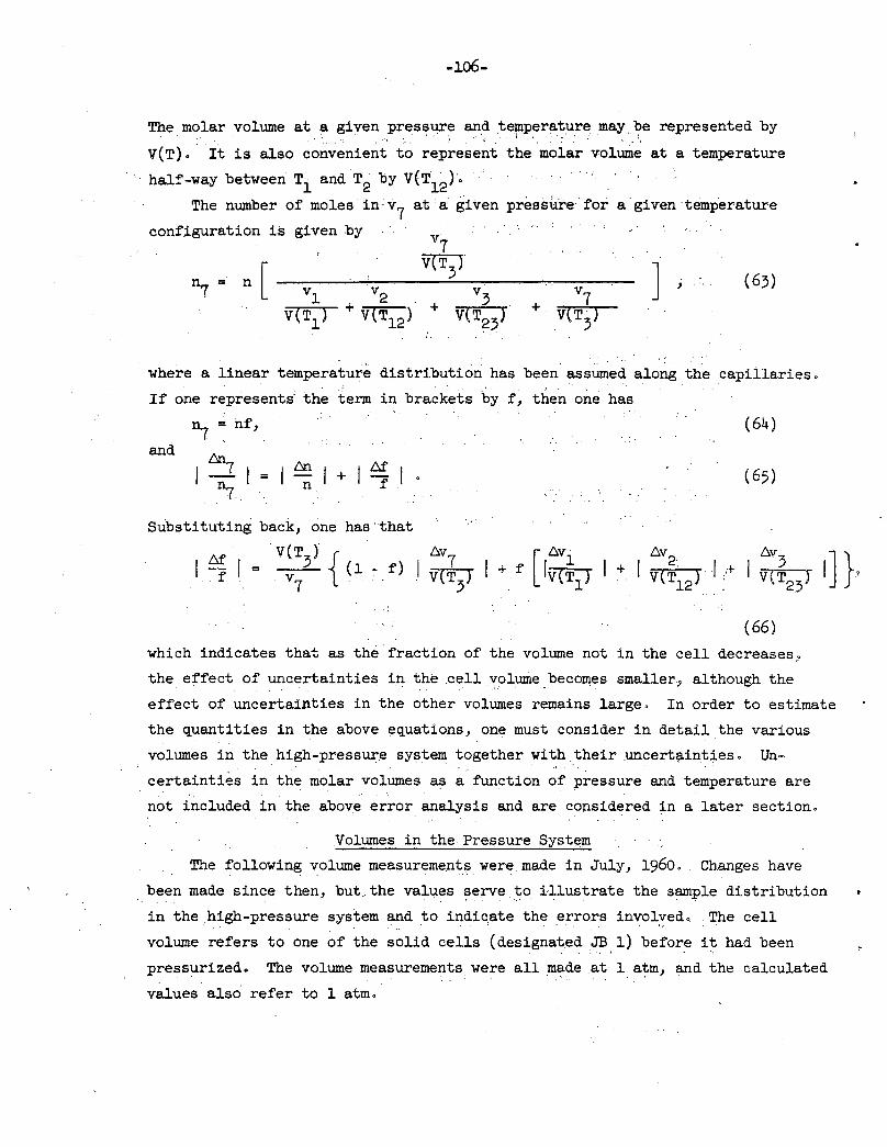
-106-

The molar volume at a given pressure and te~perature may_be represented by • .; . • ·, '•; . . ' ' • .· .;. I , '. ' • , ' . ' ~.

V(T). It is al.so convenient to represent the molar volume at a temperature

hal.f-way between T1

and T2 by V(T12) • · .·

The number of moles in v7

at a given pressure· for a given temperature

configuration is given by v7

V(T3

)

J {63) v3 . v7

, +

V(T23) + V(T

3)

where a linear temperature distribution has been assumed along the capiilaries.

If one represents· the term in brackets by f, then one has

~ = hf,' (64)

and L:m7 L:m M

1=1 1+1-fl· n7

n ( 65)

Substituting back, one has'that

M V(T3) { L::,.v7 [ L::,.vl t:,.v2, r I = --v:;-. (1 -f) I V(T3) I + f lv(Tl} I + I V(T12) I.+

(66)

which indicates that as the fraction of the volume not in the cell decreasesy

1] }9

the effect of uncertainties in the .cell yolume becomes smaller, although the

effect of uncertainties in the other volumes remains large. In order to estimate

the quantities in the above equations, one must consider in detail the various

volumes in the high-pressure system together with their uncert~int~es. Un~

certainties in the molar volumes as a function of pressure and temperature are

not included in the above error analysis and are .considered in a later section.

Volumes in the Pressure System

The following volume measurementswere made in July, 1960. Changes have

been made since then, but. the values serve, to i-llustrate the sample distribution ', ' ' I ' ' ,. ,, ,•, '•

in the high-pressure system and to indic.ate the errors involved.. The cell

volume refers to one of the s~li·d cells ( design~ted JB 1) be,~ore it had been

pressurized. The volume measurements were all m~de at 1 atm, and the calculated

val.ues also refer to 1 atm.

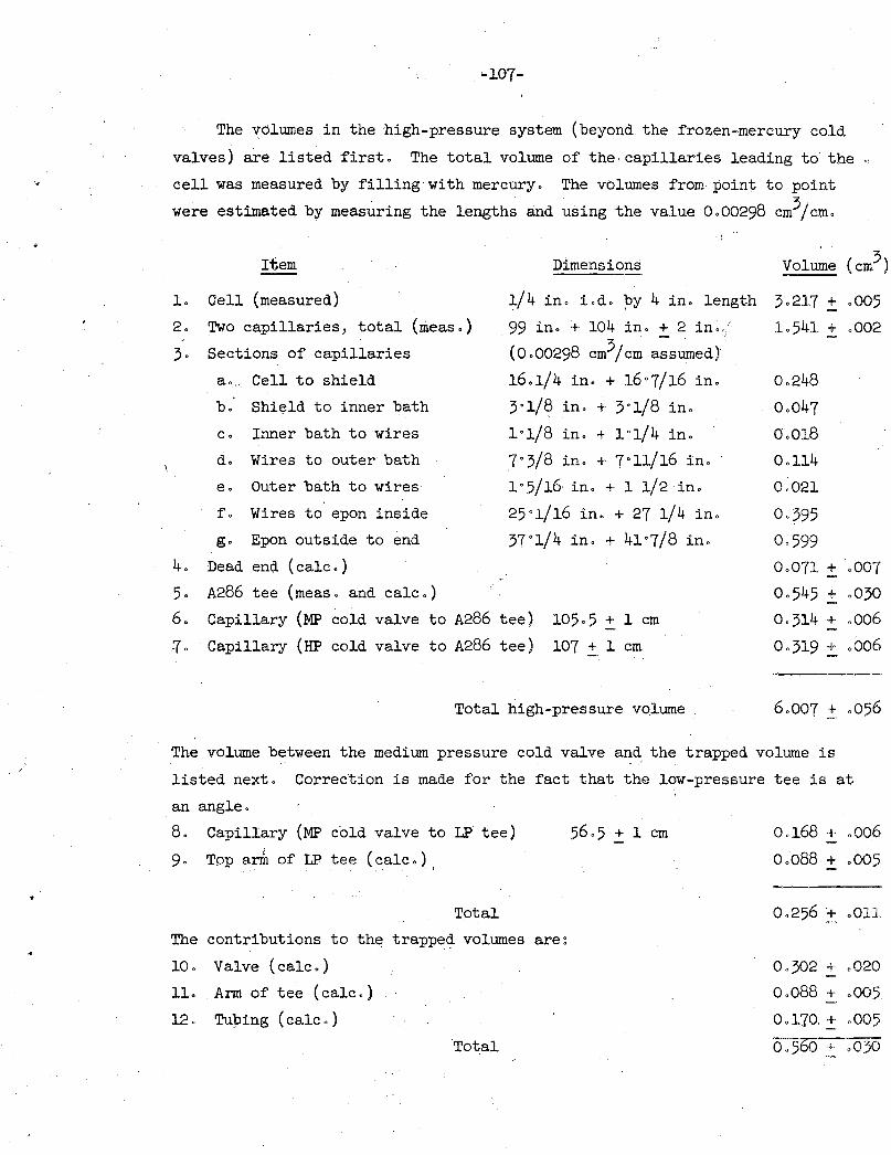
-107-

The vdlumes in the high-pressure. system (beyond the frozen-mercury cold

valves) are listed first. The total volume of the· capillaries leading to' the

cell was measured by filling withmercury. The volumes from· point to point

were estimated by measuring the lengths and using the value 0.00298 cm3/cm.

Item Dimensions

1. Cell (measured)

2. Two capillaries, total (meas.)

3· Sections of capillaries

1/4 in. i.d. py 4 in. length 3.217 ~ .005

99 in. + 104 in. + 2 in.,· 1.541 ! .002

( 0.00298 cm3 /em a~sumed),

4.

a •.. Cell to shield

b. Shield to inner bath

c. Inner bath to wires

d. Wires to outer bath

e. Outer bath to wires

f. Wires to epon inside

g. Epon outside to end

Dead end (calc.)

5. A286 tee (meas. and calc.)

16.1/4 in. + 16•7/16 in.

3•1/8 in. + 3•1/8 in.

1•1/8 in. + 1'1/4 in.

7'3/8 in. + 7•11/16 in.

1'5/16 in. + 1 1/2 in.

25•1/16 in. + 27 1/4 in.

37'1/4 in. + 41•7/8 in.

6. Capillary (MP cold valve to A286 tee)

Capillary (HP cold valve to A286 tee)

105.5 :t, 1 em

107 :t, 1 em

Total high-pressure volume .·

0.114

Oo021

0.395

0.599

0.071 :!:. .007

Oo545 .:!: .030

0.314 ::, .oo6

o 0 319 :t .oo6

The volume between the medium pressure cold valve and the trapped volume is . "·'

listed next. Correction is made for the fact that the low-pressure tee is at

an angle.

8.

9·

Capillary (MP cold valve to LP tee)

Tpp a~ of LP tee (calc.) ' . . I

Total

The contributions to the trapped volumes are~

10. Valve (calc.)

11. Arm of tee (calc.)

12. Tubing (calc.)

Ool68 + .oo6

ooo88 + .005

0 0 302 :t 0 020

0.088 + .005

0.170.! .005

0 0 560 .! .030

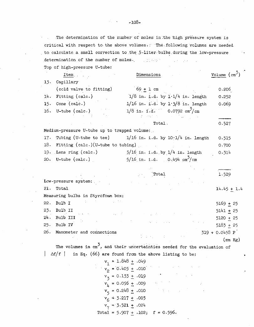
-loB-

The determination of the number of moles in :the ·high pre"ssure system is

critical with respect to. the above voliimes • :· The· following volumes are needed

. to calculate. a small correction to th~ .5-liter bulb~. during the low-pressure

determination of the number of moles.

Top of high-pressure U-tube:

Item.

13. . Capillary

(cold valve t~ fitting)

14. Fitting (calc.)

15. Cone (cal~.)

16. U-tube (calc.)

Dimensions

· 69::!:, 1 em . . .

. 1/8 in. i.d. by i·ll4 in. length

1116 in. i.d. by 1·318 in. length

118 in. i. d. b . 0792' cm3 I em

Total.

Medium-pressure U-tube up to trapped volume:

17. Tubing (U-tube to tee) 1116 in. i.d. by 10~114 in. length

18. Fitting (calc.)(U-tube

19. Lens ring (calc.)

20-. U-tube (calc.)

Low-pressure system:

21. Total

to tubing)

5116

5116

Measuring bulbs in Styrofoam box:

22. Bulb I

23. Bulb II

24. Bulb III

25. Bulb IV

in. i.d. . by 114 in. length

in. i.d. 0 •. 494 cm3 I em

·Total

.,., Volume (em-"')

0.206

0.252

0.069

0.527

0.515

0.700

0.·314

L529

5169 ::!:. 25

5141 ::!:. 25

5120 + 25

5183 :!: 25 26. Manometer and connections 319 + 0.0458 p'

(mm Hg)

The volumes in cm3, and their uncertainties needed for the evaluation of

Mlf I in Eq. (66) are found from the above listing to be:

v1 = L848 + .049

v2 = 0.405 ::!:. ~010

v3 = 0,1)3 + .019

v4 = 0.056 ! .009

v5 = 0.248 + .010 -v6 = 3~217 + .005

v7 = 3·521 + .024

Total = 5-907 ! .102; f = 0.596.

..

-109-

For the purposes of this calculation, a pressure of 4000 atm may be

taken, and the molar volume as a function of temperature may be taken as

V(T) = 16.39 + 0~0172 T cm3 • (67)

The subject of molar volumes is discussed more thoroughly;in a later section. 0 0 0 0

If one takes T1 = 300 K,.T2 = 100 K1 and T3

= 77 K, then one has T12 = 200 K,

and T23

= 88°K. The molar volumes·are V(T1 ) = 21.56 cm3, V(T2} = 18.11, V(T3

) = 17.71, V(T12) = 19.83, and V(T

23) = 17.91. For the purposes of a rough calculation

the molar volumes are close enough to be cancelled tn the equation for I ~/f I , so that one.can use

M . b.v7 f I r- I ~ <1 - f) v

7 I + v

7 < I D.v1 I + I D. v2 I + I D. v3 I ) . (68)

Substitution gives

~I . 1 r = o.oo3 + o.o13 = 0.016 (1.6%) •

Uncertainties From Other Sources

Errors .due to Temperature Uncertainty

Starting with the expression for f, one may deduce the following expression

by considering only the errors in the molar volumes., The roughequality of the

molar volumes was.used in. one s~ep to obtain a simplified expression in the

same manner as described above. We have

J ~

0 If one asstm1es a temperature uncertainty of :!::. 2 K, then, on the basis of the

linear approximation:, the voiume uncertainty at each temperature is+ 0.034 en?. Substitution in the a:bove·gives a resulting uncertainty of 0.14%•

- Errors due to the TrapPed Volume

The uncertainty here ~can be considered .as a contribution to I &/n I . Let N be the total number of'moles of gas, n be the number of moles in the

high-pressure sys'tem, v be the volume of the high-pressure system, and vT be

the trapped volume. If temperature effects are not ·considered, we obtain

v n=N--- (70)

-110-

and .,

6v~ ,.

L:m. I =·I~ I + VT

l 6v. I +·I n v v + .YT. v + VT

If one uses v = 6.007! .056 and vT = 0.560 + .030 cm3, the contribution of

the last two terms is 0.5'{o. ·

Uncertainty inN from the Low-Pressure Measurement

(71)

The ·dominant error in this case is the uncerta'inty in the volume of the

5-liter bulbs, amounting to about·0;5'fo· The sum of all of the errors considered

above is 2.8'{o. The effect of pressure in increasing the various volumes has

not been considered above, although there is reason to expect .some .cancellation

of the uncertainties in the value of f. The above uncertainty is absolute,

and it is hoped that the relative precision will be greater.

The Equation of State of Hydrogen ·

To evaluate the number of moles of hydrogen in the cell, one must know the

equation of state along and above the melting curve. The available data on

this subject are summarized below.

Bridgman38 measured the compressibility of hydrogen in 1923 at 65°C from

2000 to 15,000 kg/cm2

• The piston-displacement method was used and the gas was

compressed in contact with kerosene, lowering the accuracy of the experiments.

The•thermal-expansion data are not reported, but it is stated that the thermal

expansion of hydrogen seemed to increase somewhat with pressure. Stewart.measured

the compression of solid hydrogen and deuteritim to 20,ooo·kg/cm2 at·4.2°K, 28

connecting his data to that of Megaw. 13 Michels et al. measured the

compressibility isotherms of hydrogen and deuterium b~tween -175°C: .and + 150°C. 63 ' ' 2 '

Below room temperature, their data are all well below 1000 kg/em • Accurate

P-V-T data on normal hydrogen from.O to 200 atm between 35°K and 300°K have 64

been obtained by Johnston and coworkers.

The melting c1,1I've of hydrogen was determined l?Y· Simon, Ruhemann, and

Edwards i.n 1930, 65 . and, more recently, Mills and Grilly have determined the

melting curves of hydrogen, deuterium, and tritium. 66 Bart.holome measured . . . . . 2

the volume of the liquid ~d the volume chang;e on melting up to 152 kg/ em

(18.24°K) with hydrogen and up t<? 98.7 kg/cm,2 (20.97°K) with deute:r;ium. 67

His data indicate that the entropy of me_lting decrea~es gradu~lly as the

.... pressure increases .•

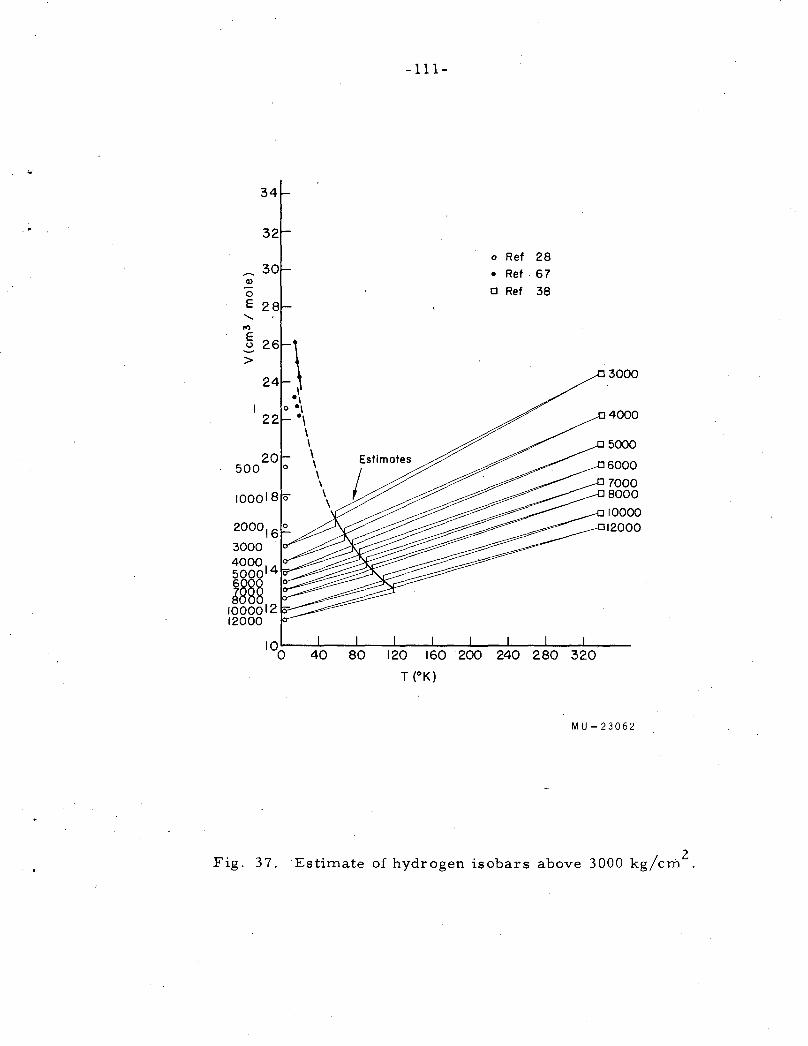
Q)

0 E

....... ,., E u

>

400014 5000

j§§§ 1000012 12000

-111-

o Ref

• Ref.

a Ref

28

67 38

3000

4000

5000

6000

7000 8000

10000 12000

10o 40 80 120 160 200 240 280 320

T (°K)

MU-23062

Fig. 37. Estimate of hydrogen isobars above 3000 kg/cm2

.

-ll2-

The simplest way of estimating the equation of state in the region of

interest (20 to 120°K, 1,000 to 12,000 kg/cm2 ) is to plot the data of Bridgman

and Stewart on a molar-volume-versus-temperature graph and then draw linear

isobars. This has been done in Fig. 37· Since the melting temperature is

known as a function of pressure, the molar volume at which melting occurs may

be obtained on the basis of the above approximation. An upper limit to the

volume change with melting may be calculated by using a constant entropy of

melting in the Cl~usius-Clapyron equation along with the melting ... curve data.

A value of 2.00 cal/mole/°K was taken, and the above calculatio~ was carried

out.. These volume discontinuities were added to the melting curve in Fig. 37,

.as may be seen. The linear interpolation above 3000 kg/ cm2 may be off by

10% or more, so that it will be necessary to determine the equation of state

in the region of interest for the present experiments.

Below 3000 kg/cm2 it is certain that the isobars are curved, and there

is very little data on which to base interpolations, so that no attempt has

been made to estimate the P-V-T properties in this regioi!'. Measurements of

the equation of state will be required in this region also. Since the P-V-T

measurements can be made in the calorimeter in the same cell to be used for

the heat-capacity measurements and to•the same precision obtainable in the

heat capacity work, no special problems arise from this difficulty. Fig. 37

may be used to obtain an estimate of the highest pressure obtainable by the

blocked-capillary method •.. ·Assuming that 12,000 kgj cm2 is the highest pressure

that can safely be generated, the linear interpolation indicates that the

molar volume of the fluid at the melting point is 13.3 cm3. At 4.2°K, this

corresponds to a pressure of about 6,000 kg/cm2 • To obtain higher pressures,

one may have to use a method suggested by Nesbitt and Fiske68 of the General

Electric Co., Schenectady, N. Y. An insulated heater wire (such as Formvar­

covered manganin) could be threaded into the capillary from the room-temperature

end down to the cell. By keeping the temperature in the capillary above the

melting point, it would be possible to raise the pressure in the cell to the

value obtainable at the other end of the system. Since this technique would

probably be trickY- to apply, it seems best to obtain as much data as possible

by using the blocked-capillary method first.

Extrusion of Hydrogen Through Capillaries

The extrusion pressures of hydrogen through a hole of 1/8 in. diam. and

unspecified length (probably 1/2 in., as estimated from drawing) were measured

by Stewart to be 240 kg/cm2 and 290 kg/cm2 , respectively. 27 These data may be

..

-113-

used to obtain a rough estimate of the highest pressure differences that may

be used in the present experiments without having extrusion of the hydrogen in

the capillaries, and hence, failure of the blocked-capillary method. The

analysis of the stress-strain pattern of a solid in a tube with a pressure

at one end is analogous to the analysis of the viscous flow of a fluid in a,

capillary. Consider the case of an incompressible solid. Let R be the

radius of the capillary, S be the tangential stress on a curved surface

perpendicular to a radius of the capillary, G be the modulus of elasticity

in shear of the hydrogen in the capillary, and 1 be the length of the

capillary sustaining the pressure difference p. It can be shown that the

maximum shearing stress occurs at the radius of the capillary, and is expressed

by PR s = 21

2 If the yield pressure is 240 kg/em for a 1/8-in. diameter and 1/2-in.

(72)

length, then the above equation allows the yield pressure for a 0.025-in.

diameter and 3-in. length (a practical situation in the present experiments)

to be estimated as 7200 kg/cm2

. Since the solid is actually compressible,

this estimate is too large. On the other hand, one would expect the solid

to.become harder as the pressure is increased.

A calculation may be carried out which takes the compressibility of the

solid into account. Aside from.being rather complicated, the result depends

on the value of the shear modulus, G, which cannot be evaluated.accurately

enough from the available data, and whose pressure dependence is unknown.

Although it seems unlikely that extrusion in the capillaries will be a problem,

one should test for the effect in the first runs by following the pressure on

the room-temperature side as the capillary is frozen and the cell cooled.

-114-

VII. THEORETICAL CONSIDERATIONS .. -.,

Introduction

· Although no high-pressure heat-capacity data are yet available for analysis,

a fair amount of 1-atm data on the heat capacity of solid hydrogen and deuterium

has appeared in the literature during the past two years. Since the phenomena

occurring at 1 atm will be relevant to high-pressure studies, and since the data

are interesting in themselves, it was desirable tq consider these data and the

theoretical interpretations which have been made.

The modern data on the anomalous heat capacity of solid hydrogen and

deuterium have been published in four papers from two laboratories •. In 1954

Hill and Ricketson published data on solid hydrogen between 2 and 14°K on

samples containing 0.5, 7, 25, 41, 56, 66, and 74% o-H2 .8

At the two higher 0 concentrations, the data were extended to 1.15 K. and a A anomaly was discovered.

. 0 In the next year, the same authors extended the measurements to 0.2 K and found

that the A. anomaly did not occur below about 60% o-H2 concentration. 9 In 1957

Gonzalez, White, and Johnston published data on solid. deuterium between 0.3

and 13°K on samples containing 3, 14-5, 18.5, and 33.3% p-D2 •14 No A. anomaly

was discovered because the concentration of p-D2

was not high enough. In 1959

Hill and Lounasmaa obtained data on the lattice 'heat capaCities of solid

hydrogen and deuterium by reducing t~e o-H2

and p-D2 impurity concentration

as much as possible. 69. By having the conversion catalyst in the sample and

equilibrating for'2 hr at the triple point before freezing the sample and taking

measurements, they obtained a nominal o-H2 concentration of 0.02%, and nominal

p-D2 concentrations of 1.5 or 2.15%, depending on the temperature of equilibration.

The solid-hydrogen data were fitted by a function of the type, C · = AT3 + BT5, p

as were the deuterium data after the anomalous contribution of the p-D2 was

subtracted empirically.

The-interpretation of the above data has been the subject of several other

papers. Tomita applied the Bethe approximation in the statistical treatment of

the cooperative phenomenon and calculated the temperature dependence of the peak

of the anomaly with respect to o-H2

concentration. 10 The theory predicted the

lowest concentration for the occurrence of the A. anomaly to be 16.7%, as compared

with the experimental value of 60%.

Nakamura70 considered the valence, electrostatic quadrupole,. and London

dispersion forces in the pairwise interaction of adjacent ortho molecules and

ce:a.lculated the magnitude of the high temperature "tail" of the anomaly, using

~-115-

Hill and Ricketson's data.8

This calculation applied only to the region -2

where the anomalous heat capacity was proportional to T • Nakamura also

calculated the pairwise energy levels for quadrupolar interaction and_compared a!. . 8

the predicted heat capacity with Hill and Ricketson's 7~ data. The data were

about a factor of two larger than the theoretical result. He. then fitted the

discrepancy with the expression for a two-level anomaly (upper-level'degenerate)

proportibnal to the o-H2 concentration. (The pairwise energy was proportional

to the square of the concentration.) A fit was obtained by using a splitting -16 ( of 2 x 10 ergs per molecule since Nakamura seems to have counted some of

the o-H2

molecules twice in this calculation, the numerical value is in doubt).

In order to explain the contribution dependence on the first power of the

o-H2 concentration, Nakamura postulated a splitting of the rotational levels

by the lattice motion of the molecules. In a later paper, Nakamura and

Uryu calculated the quenching of the rotational states of ortho hydrogen

in the solid .state by using·the Einstein model for lattice vibrations and . -16 71 obtained a splitting of 0.72 x 10 ergs between theM= 0 and+ 1 levels.

In the present work, it was of interest to reexamine Nakamura's

conclusions in the light of all of the recent data. From the experimental

point of view, his result was based on a single experiment, and might be

altered by small discrepancies. From the theoretical point of view, Nakamura

did not explicit~y consider isolated ortho molecules, isolated pairs of ortho

molecules, and more complicated configurations at the 7% concentration. On

this basis, it was still of interest to determine whether a realistic cal­

culation based on the angular potential energy between ortho molecules could (

account for the size and shape of the heat-capacity anomaly.

At high pressures the different shape and repulsive energies between ortho­

ortho and ortho-para pairs· becomes important, and one might expect that such

effects can no longer be neglected in calculating the splitting of the ortho­

hydrogen sublevels. The energy-level system of a pair of ortho molecules in

solid hydrogen was calculated considering these effects. The case of three

ortho molecules in a row was also treated in the quadrupolar approximation.

The two models had appreciably different level systems and heat capacities.

The energy-level system for pairwise interaction was calculated as a function

of intermolecular separation, and it was found that, although only the quadrupole

interaction is important at 1 atm, valence forces become important at 5000 atm.

The experimental data at various o-H2 and p-D2

concentrations were compared

with the calculations, and the present understanding of the situation was

discussed.

-116-

Interaction Between Two Hydrogen-Molecules

The various contributions to the interaction-between two hydrogen molecule.s

have been discussed by Hirschfelder, Curtiss, and Bird. 52 Three effects are

important in the-angular dependence of the intermolecular potential. These

are (a.) the chemical or valence energy (sometimes called the exchange

repulsion), (b) the electrostatic quadrupole-quadrupole interaction, and

(c) the inverse sixth-power dispersion energy. The inverse•eighth-power

dispersion energy is small, and its angular dependence is considered negligible

by Hirschfelder et al.52

Because of its convenience, de Boer's theoretical result for the valence

energy31 is used. Over the range 4a to lOa (a = 0.529A), de Boer's result 0 0 0 .

was expressed as

V(va1) = 2 •78 =: [ e-L87ra/a0 +e-L87rbcfa0 + e-L87raafa0 +e-L87rbJa0 J, (T?)

where nuclei ab and cd form the two molecules. The following approximation,

recommended by de Boer for the region 6a to 8a , shows the angular dependence 0 0

explicitly:

2 { a 11 a 13 vl(val) =: 48,000 (r0

) + 129,360 (r0

) [13 cos2

Qab + 13 cos2

Qed - 2] 0

+ 2 { sin Qab sin Qed cos (¢ab

4 4 + ~.::255 cos Q ab + :~255 cos Q cd }

The electrostatic,quadrupole-quadrupole interaction is given by52

+2

(74f

(75)

-117-

where Q is the cylindrically symmetric quadrupole moment,. about the internuclear

axis. Harrick and Ramsey have measured the quadrupole moment of hydrogen by a

molecular-beam microwave-resonance method. 72 They obtained a value for Q/e of -16 ·2 . - ·. ' ·.

0.220 x,lO em relative to the internuclear axis. This numerical value pertains

to the convention used by Hirschfelder et al.53

The dispersion potential at large separation may be repre_sented as

follows: 52 ' 73

v(dis) = _ C(G , a

where Ga' ¢a; Gb, ¢b refer to the intermolecular axis, and

(76)

2 2 . (77) + 3(B - C) cos Ga + 3(B' - C) cos Gb + (B + B' + 4C)

Here we define ·

h A = 4 a 11 (a) a

11 (b)

v 11 (a) v11

(b)

v11 (a) + v11

(b)

. (a) v (b). h VII

B' (a) a.L (b) JL B = = 4 °11 (a) +'JL (b) VII

and

h vl. (a) v_L ( b;) _ c = 4 aj_ ( a) a l_ (b)

vl. ( a) + v 1. (b)

(78a)

( 78b)

(78c)

where a11

and a_l , are the polarizabilities along and perpendicular to the

molecular axis, respectively, and v11

and vl_ are the fundamental frequencies

for (electronic) vibrations_ along and perpendicular to the.molecular axis, the

latter being doubly degenerate.

If we assume that molecules a and b are of the same kind, and set

v11

= l = . v = I/h,' where I is the ionization potential, 52 Eqs. ( 78) reduce to

A = 2

aft I

8 , B = B' =

-ll8-

and c = 8

2 a..L. I

8

If the anisotropy of polarizability, K, is defined by

a" - aJ. K = ' a, + 2 aJ.

the combinations appearing in Eq_. (77) become

(A - 2B + C) ~2 ell ~ a_L y Ia? K2 ' = =

8

I a..La I a 2

B - C ( a/1 a - aj_ ) "" K ' =

8 8

and

2B + 4C = 3 2 4 I a .

(79)

(8o)

(8la)

(8lb)

(8lc)

The approximation a~~ a seems justified for our purposes since we have

a..L = (1 - 1/3 K) a and K ~ 0.1. In order to replace ra2 in Eqs. (81)

by a more empirical q_uantity, the London force between spherically

symmetric molecules, - 3/4 It:i;r6, may be compared with the coefficient

of the empirically fitted Lennard-Janes 6-12 potential, 4e [ (i)12 - ( ~ )6] , . r r which gives the result: ra2 = 16/3 ecr2 . For hydrogen, we have e/k = 37.00°K,

and CJ = 2.928A. If we replace CJ by 5·55a , the above eq_uations may be com-o bined and substituted into Eq_. (76) to g~ve a usable expression for the

angular dependence of the London inserve sixth-power dispersion energy:

(a· ) a 6 [ 2 2 v 1s = -29,000 e ( ro ) 4 + 2K(cos ga +cos gb)

+ 2/3 k2

{sin Qa sin Qb cos (¢a - ¢b) - 2 cos ga cos gb }2

] • (82}

The value of K used for these calculations was 0.1173. 52

The inverse eighth-power dispersion energy may be expressed as52

V(dis,8) = _116 e2

· ( ao ) 8 a r (83)

0

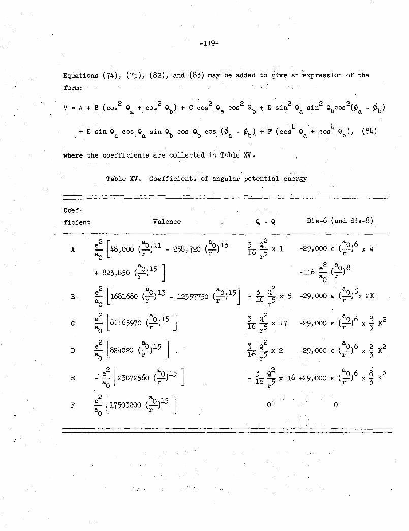
-119-

Equations (74·), (75):, (82); and (83) may be added to give an :~xpression of the

form:

where the coefficients are collected in Table xv.

Table xv. Coefficients of angular potential energy

Coef-

ficient Valence Q - Q Dis-:-6 (and dis-8)

e2

[48,000 a a 3 Q2 ao 6

A (_£)11 - 258,720 (_£)13 j]) 5 x1 -29,000 € (--) X 4 ao r r r r

+ 823,850 (:0 )15 J 2 a 8 -116 ~ (_Q)

ao r

2[ · a a J 3 Q2 ( ao)6x 2K B ~ 1681680 (_Q)13 - 12357750 (_Q)15 5 -29,000 € ao r r -I55x r r

c e2

[81165970 (a0 )15 J 3 Q2 -29,000 € ( ao)6 x ~ K2 lb 5 X 17 ao r r r 3

D e2 [824020 (a0)15 J 3 Q2 -29,000 € to)6 X~ K2

ao r lb5 X 2 r 3 · r

E -· e2

[23072560 (a0 )15 J 3 Q2 to)6 X~ K2 . - lb 5 X. 16 +29,000 € ao r r r 3

F e2

[17503200 (a0 )1 5 J 0 0 ~

a0 r

-120-

Application of Perturbation Theory. to Pairwise .Interac_t:i,or;l

A problem relating to the anomalous heat-capacity effects. in.solid hydrogeh

that can be treated with some degree of realism from the theoretical point of

view is the pairwise interaction of two6rtiio molecules, each having eleven

para-hydrogen neighbors. Since each ortho-hydrogen molecule (J = 1) has three

degenerate orientational eigenstates in the absence of a perturbation, a pair

of ortho molecules has nine degenerate states. Application of first-order

perturbation theory to this problem yields the correct combinations and eigen­

values of the nine states under the applied perturbation. 74 Mathematically,

the procedure involves the calculation of the matrix elements of the 9 by 9 . array and the solution of the resulting secular equation .•

·The potential of interaction of.the two ortho molecules is:given by

Eq. (84), as is _the potential of interaction between each ortho molecule and

each of its para neighbors. The unperturbed wave functions·may he taken as

follows:

Ortho Molecule at a

1jra_ = ! -·{~. sin Q 1 2 1t a

cos ¢a (85a)

ta = !"f?: cos Q (85b) 2 2 1( a

1jra = !~ sin Q sin ¢ (85c) 3 2 1( a a

Ortho Molecule at .b

1jrb = !~ sin Qb cos ¢b (85d) 1 2 1(

1jrb = ! -fl. 2 2 1(

cos Qb (85e)

1jrb =! -w 3 .. 2 1(

sin Qb sin ¢b, (85f)

with all para states being represented by 1jr~ = lj~. For the rest of the . . ~

discussion, a state such as t~ 1jr~ will be referred to as (13).

The interaction between an ortho molecule and one of its para neighbors

is considered first. The three zeroth-order states will be of the form 1jr~ ~'

..

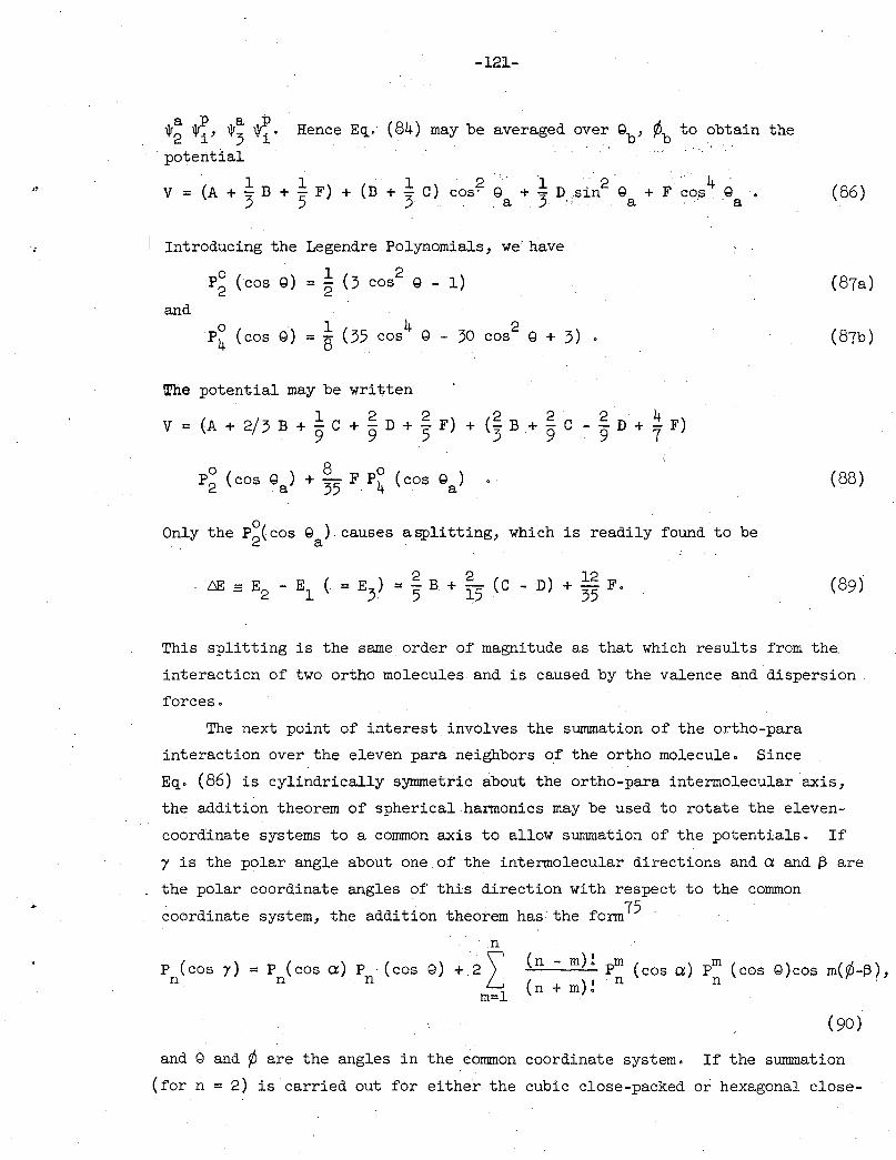
-121-

1Jr~ ~' w; ¥i· Hence Eq. (84) may be averaged over Qb' ¢b to obtain the

· potential

V = (A + 5 B +~F) + (B + 5 C) cos? Qa + ~- D,sin2

Qa + F cos4

Qa

Introducing the Legendre Polynomials, we-have

P~ (cos Q) = ~ (3 cos2

Q - 1)

and 0 . 1 4 2

P4 (cos Q) = 8 (35 cos Q - 30 cos Q + 3) •

The potential may be written

V = (A + 2/3 B + ! C + g D + g F) + (g B + g C - g D + ~ F) . 9 9 5 3 . 9 9 7

Only the P~(cos Qa) causes a~litting, which is readily found to be

(86)

(87a)

(87b)

(88)

(89)

This splitting is the same order of magnitude as that which results from the.

interaction of two ortho molecules and is caused by the valence and dispersion

forces.

The next point of interest involves the summation of the ortho-para

interaction over the eleven para neighbors of the ortho molecule. Since

Eq. (86) is cylindrically symmetric about the ortho-para intermolecular axis,

the addition theorem of spherical harmonics may be used to rotate the eleven­

coordinate systems to a common axis to allow summation of the potentials. If

y is the polar angle about one of the intermolecular directions and a and ~ are

the polar coordinate angles of this direction with respect to the common

coordinate system, the addition theorem has the form75

.n

P (cos y) = P (cos a) P (cos Q) + 2 \ n n n L

m=l

( n - m)! pm ( ) m ( ) (¢ ) cos a P cos Q cos m -~ , (n + m)! n n

(90)

and Q and ¢ are the angles in the common coordinate system. If the summation

(for n = 2) is carried out for either the cubic close-packed or hexagonal close-

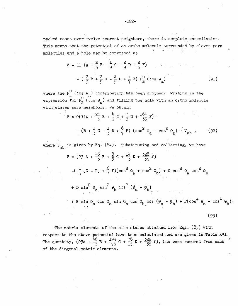
-122-

packed cases over twelve nearest neighbors, there is complete cancellation.

This means that the potential of an ortho molecule surrounded by eleven para

molecules and a hole may be expressed as

2 1 2 . 2 V = 11 (A + - B + - C + - D + - F) . 3 9 9 5

- ( ~ B + ~ C - ~ D +~F) P0 (cos G ) 3 9 9 7 2 a

where the P~ (cos Ga) contribution has been dropped. Writing in the

expression for P~ (cos Ga) and filling the hole with an ortho molecule

with eleven para neighbors, we obtain

. V = 2(llA + 23 B + ~ C + 1 D + 164 F) -3 3 3 35

(B + ~ c - ~ D + ~ F) ( 2 A 2 A ) v - 3 3 7 cos ~a + cos ~b + ab '

where Vab is given byE~. (84). Substituting and collecting, we have

V = (23-A + 46 B + ~ C + 14 D + 328 F) 3 3 3 35

1 6 2 2 2 2 -( '3 [C - D] + '7 F)(cos Qa + cos Gb) + C cos Qa cos Gb

D . 2 A • 2 A 2 (¢ ¢ ) + s~n ~a s~n ~b cos a - b

(91)

(92)

(93)

.. The matrix elements of the nine states obtained from E~s. ( 85) with

respect to the above potential have been calculated and are given in Table XVI. . . . 46 193 78 322 • The ~uant~ty, (23A + ~ B +

75 C +

15 D +

35 F), has been removed from each

of the diagonal matric elements.

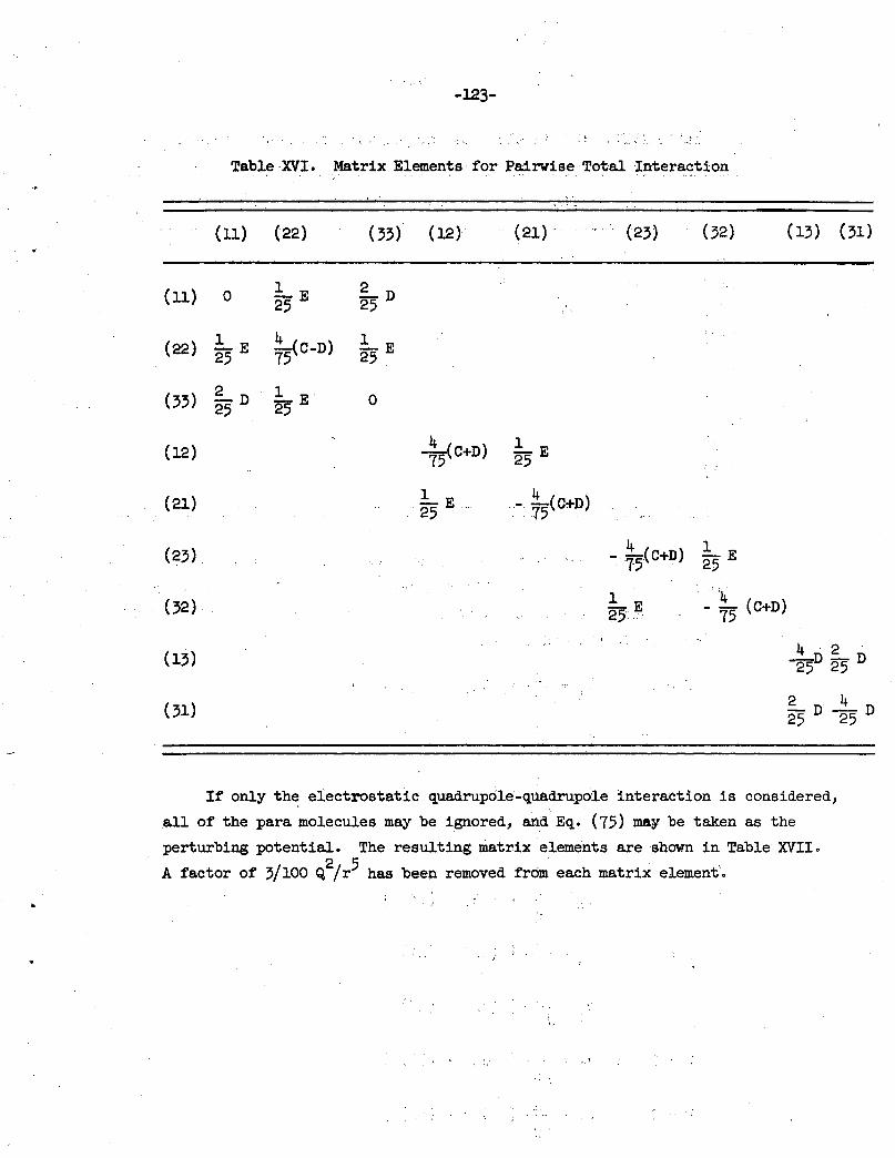
·123-

,. ' . . .~. ..: ..

Table XVI. Matrix Elements· for Pairwise Total Interaction

(11) (22) (33) (12) (21) . (23) (32) (13) (31)

(11) 0 1 25 E

2 25 D

(22) 1 4 1 25 E -(C-D) 25 E 75

(33) 2 l_E 0 25 D 25

(12) 4 75(C+D) 1

25 E

(21) 1 25 E ..

4 - 75(C+D)

(23). 4 ~ 75(C+D)

1 25 E

(32). l_E 4 - - (C+D) 25 .. 75

(13) 4 . 2 . 25D 25 D

(31) 2 4 25 D -25 D

If only the: electrOstatic quadrupole·-qu.a.drupole interaction is considered,

all of the para molecules may be ignored, and Eq. (75) may be taken as the

perturbing potential. The resulting matrix elements are shown in Table XVII.

A factor of 3/100 Q,2/r5 has been removed from' each matrix element'.

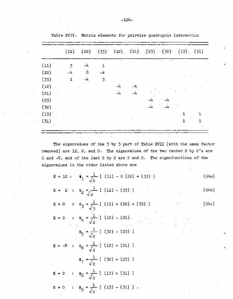
-124-

Table XVII. Matrix elements for pairwise quadrupole interaction

(11) (22) (33) (12) . (21) :(23} .. (32)· '(13) .. (31)

(11) 3 -4 .1

(22) -4 8 -4 (33) 1 -4 3

(12) -4 -4 (21) -4 -4 (23) -4 ' -4

(32) -4 -4 (13). 1 1·

(31) 1 1

The eigenvalues of the 3 by 3 part of Table XVII (with the·· same factor

removed) are 12, 2, and o. The eigenvalues of the two center 2 by 2's are ' 0 and -8, and of the last 2 by 2 are 2 and o. The eigenfunctions of the

eigenvalues in the order listed above are

E = 12 ' 1 (11) - 2 (22) + (33) (94a) t =- [ ' 1 .f6

1 (11) - (33) ] (94b) E = 2 1jr = - [ 2 .[2

1 (11) + (22) + (33) ] (94c) E = 0 ·•· 1jr =- [ .

3 .[3

1 (12) - (21). E = 0 1jT4 =- [ .[2

1 ( 32) - ( 23) ] 1jT =- [ 5 .[2

E = -8 1 (12) + (21) ] "ljr6 =- [

.[2

1 ( 32) + (23) ] 1jT =-- [ 7 .[2

E = 2 1 w8 = - r

.[2 (13) + (31) ]

1 ( 13) .;. ( 31) ] E = 0 1jr =- [ 9 .[2

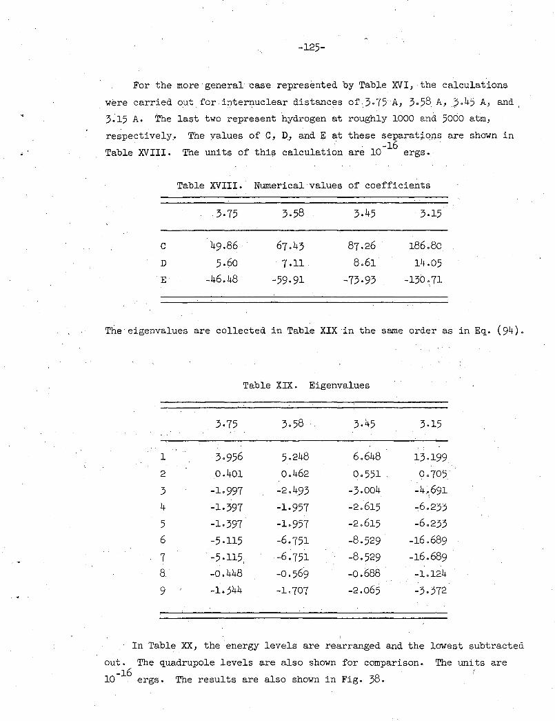
-125-

For the more-general case represented by Table XVI, the calculations

were carried out for internuclear distanees of-3.75A, 3.58.A, ;.45 A, and,

3.15 A. The last two represent hydrogen at roughly 1000 and 5000 atm,

respectively .•

Table XVIII.

c D

E

The values of C, D, and E at these separat;Lon.s are shown in -16

The units of this calculation are 10 ergs.

Table XVIII. Numerical values of coefficients

3-75 3.58 3.45 . 3·15

49.86 67.43 87.26 186.80

5-60 7.11 8.61 14.05

-46.48 -59·91 -73·93 -130.71

The eigenvalues are. collected in Table XIX in the same order as in Eq. (94).

Table XIX. Eigenvalues

3·75 3.58 3·45 3-15

1 3·956 5-248 6.648 13.199

2 0.401 0.462 0.551 0.705

3 -1.997 -2.493 -3.004 -4.~691

4 -1.397 -1.957 -2.615 ~6.233

5 -1.397 -1.957 -2.615 -6.233

6 -5.115 -6.751 -8.529 -16.689

7 -5.115 -6.751 -8.529 -16.689 ,,

8. -0.448 -0.569 -o.688 -1.124

9 -1.344 -1.707 -2.065 -3·372

In Table XX, the energy levels are rearranged and the lowest subtracted

out. The quadrupole levels are also shown for comparison.

lo-16 ergs. The results are also shown in Fig. 38.

The units are (

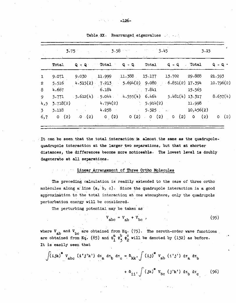
. -· '. -126-

-Table. ;XX. Rearranged_ ,eigenvalues

,,

3·75

Total Q -: Q. ··Total Q - Q Total Q - Q Total Q - Q •

l 9·071 9·030 .11.999 11.388 15.177 13.702 29.888 21.593

2 5·516 4 ·515(2) . 7.213 5·694(2) 9.080 . 6.851(2) 17 ·394 10.796(2)

8 4.667 6.184 7.841 15.565

9 3·771 3.612(4). 5.044 . .4.555(4) 6.464 5.481(4) 13.317 8.637(4)

4,5 3·718(2) 4.794(2) 5·914(2) 11.998

3 3oll8 4.258 5.525 '. 10,456(2)

6,7 0 (2) 0 (2) 0 (2) 0 (2) 0 (2) 0 (2) 0 (2) 0

It can be seen that the total: interaction :is .almos.t. the same as the quadrupole­

quadrupole interaction at the larger two separations, but that at shorter

distances, the differences become more noticeable. The lowest level is doubly

degenerate at all separati~ns • • t"

· · · Linear _Arrangement of Th~ee Ortho Molecules

The preceding calculation is readily extended to the case of three ortho

molecules along a· line {a,·· b, c), Since the quadrupole interaction is a good

approximation t.o the' total interaction at.· one atmosphere, only the quadrupole .·

perturbation energy will be considered.

The perturbing potential may be taken as

Vb =Vb+Vb ·, a c a c (95)

(2)

where Vab and Vbc are obtained from Eq. (75), The zeroth-order wave functions

are obtained from Eq. (85) and 'ir~ v; V~ will be d_enoted by (132) as before. .•

It is easily seen that

-

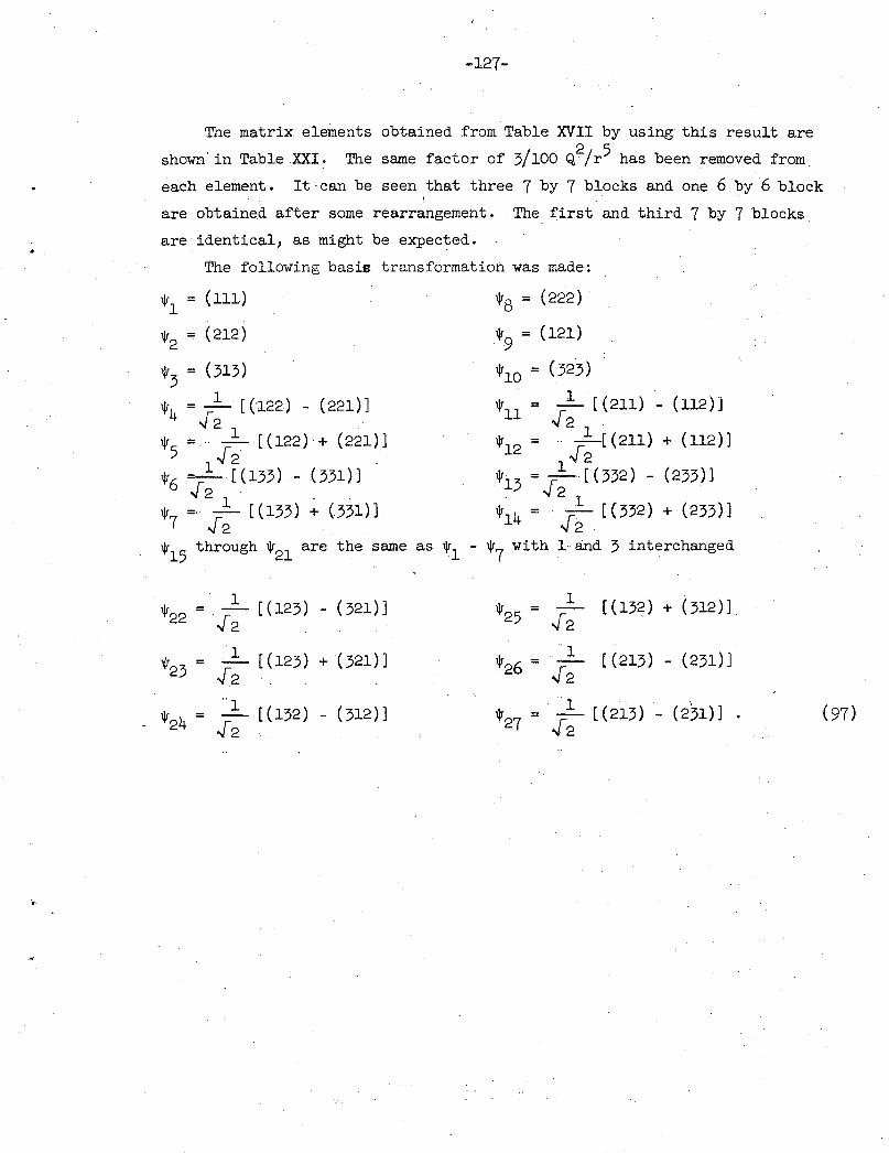
-127-

The matrix elements obtained from Table XVII by using this result are

shown· in Table XXI. The same factor of 3/100 Q2/r5 has been removed from

each element. It·can be seen that three 7 by 7 blocks and one 6 by 6 block I

are obtained after some rearrangement. The first and third 7 by 7 blocks

are identical, as might be expected.

The following basis transformation was made:

\jr = (111) 1

\jr2 = (212)

\jr3 = (313)

\jr4 = .1:_ [ ('122) - (221)] .[2 1

\jr =.··- [(122) + (221)] 5 1.[2 .·

\jr6 =-·- [ (133) - (331)] .[2 1 '

\jr =· - [(133) + (331)] 7 .[2 .,

1Vs = (222)

'9 = (121)

,10 = (323)

,11 = .1:_ [(211) - (112)] .[2 1

1jr = .. -[ (211) + (112)] 12 .[2

1 1jr =-[(332)- (233)] 13 .[2 '

1jrl4 = .. .[~ [(332) + (233)]

\jr15

through w21 are the same as w1 - w7

with l-and 3 interchanged

.l:_ [(123) - ( 321)] \jr25 = 1 [ (132) + ( 312)] \jr22 = -

.[2 ' .f2 .. ..

1 o/23 = .l:_ [ ( 123) + ( 321)] ,26 = - [(213) - (231)]

.[2 . .f2 . .

o/24 = .l:_ [(132) .[2

- ( 312)] ,27 = .[~ [ (213) - (231)] . (97)

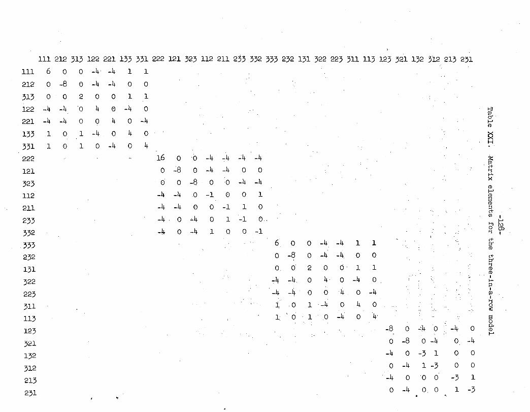
111 212 313 122 221 133 331 222 121 323 112 211 233 332 333 232 131 322 223 311 113 123 321 132 312 213 231

111 6 0 0 -4 -4 1 1

212

313

122

221

133

331

222

121

323

112

211

233

332

333

232

131

322

223

311

113

123

321

132

312

213

231

0 -8 0 . 0

-4 -4 -4 -4 1 0

1 0

0

2

·o 0

1

1

-4 -4 0

0 0 1

4 0 -4 0 4 0

-4 0 4

0 -4 0

0

1

0

-4 0

4 16 0

0 -8

0 0

-4 -4 -4 -4 -4. 0

-4 0

·o 0

-8

0

0

.;;.4

-4

-4 -:4 .:4

-4 -4 0

0 0 -4 -1 0 0

0 -1 1

0 1 -1

1 0 0

-4 0

-4 1

0

0

-1

6 0 0 -4. -4 0 -8 0 -4 -4 0 0 2 0 0

-:4 -4 0 4 0

-4 -4 . 0 0 4 1 0 1 -4 0

1 0 1 .· 0 ~4

1 1

0 0

1 1

-4 0

0 -4 4 0

0 4·

:.:,·

-8 0 ..:4 0

0 -8 0 -4

-4 0 -3 1

-4 0

0 -4

0 0

0 -4 1 -3 0 0

-4 0 0 0 -3 1

0 -4 0 0 1 -3 •:

8

~ 1-' (!)

~ H

! ., 1-'­>< (!)

1-'

~ ~ Ul I

~~ '"'i I

c+ ::r (!)

c+ ::r ., (!) (!) I

1-'-::s I PJ I ., ~

5 p.. (!)

1-'

•

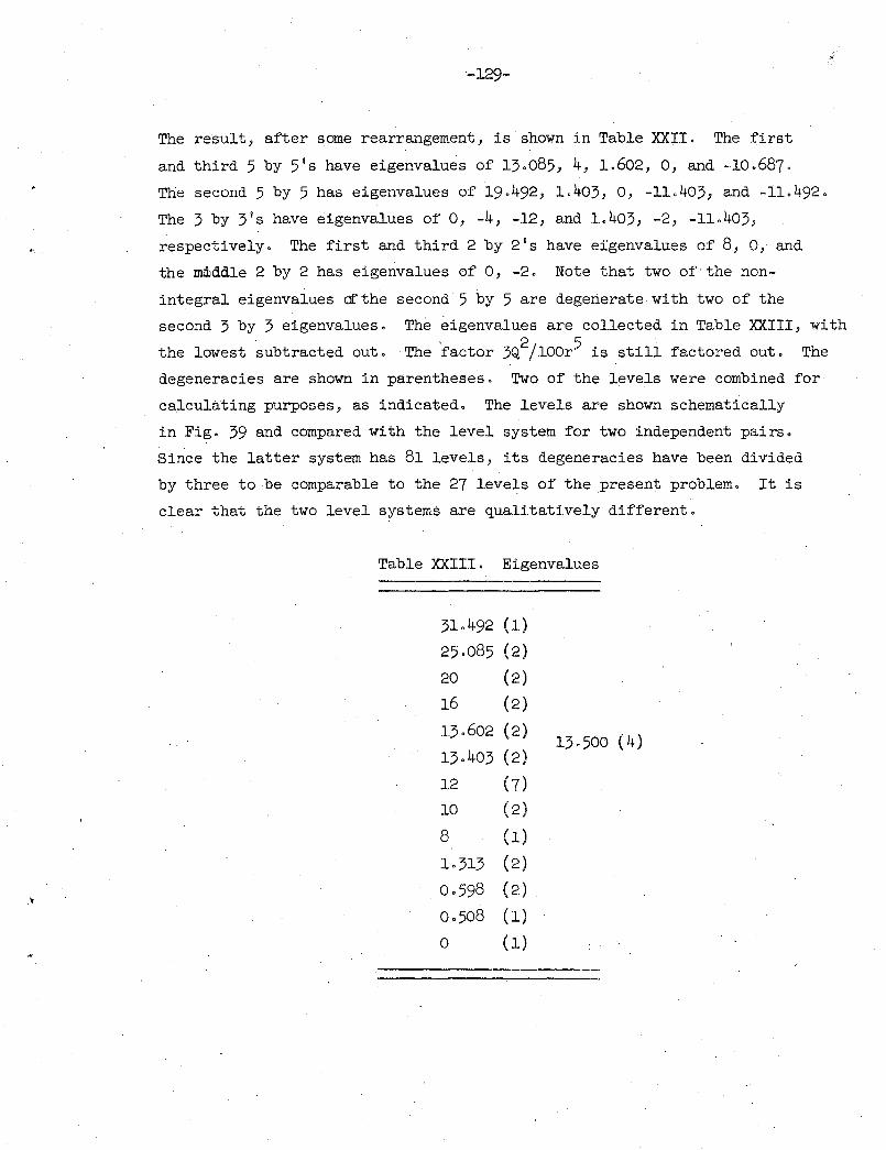
-129-

The result, after some rearrangement, is shown in Table XXII. The first

and third 5 by 5's have eigenvalues of 13.085_, 4, 1.602, 0, and -10.687.

The second 5 by 5 has eigenvalues of 19.492, 1.403, o, -11.403, and -11.492.

The 3 by 3's have eigenvalues of O, -4, -12, and 1.403, -2, -11.403,

respectively. The first and third 2 by 2's have eigenvalues of 8, 0, and

the mdlddle 2 by 2 has eigenvalues of 0, -2. Note that two of·the non­

integral eigenvalues afthe second 5 by 5 are degenerate with two of the

second 3 by 3 eigenvalues. The eigenvalues are collected in Table XXIII, with

the lowest subtracted out. The factor 3Q2/lOOr5 is still factored out. The

degeneracies are shown in parentheses. Two of the levels were combined for

calculating purposes, as indicated. The levels are shown schematically

in Fig. 39 and compared with the level system for two independent pairs.

Since the latter system has 81 levels, its degeneracies have been divided

by three to be comparable to the 27 levels of the present problem. It is

clear that the two level systems are qualitatively different.

Table XXIII. Eigenvalues

31.492 (1)

25.085 (2)

20 (2)

16 (2)

13.602 (2) 13.500 (4)

13.403 (2)

12 (7)

10 (2)

8 (1)

1.313 (2)

0.598 (2)

0.508 ( 1)

0 (1)

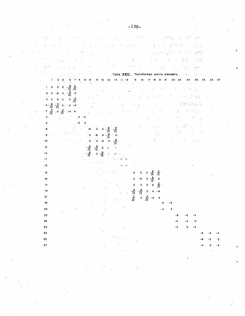
-130-

'•

. To ble :::X:X:O:. Transformed matrix elements.

2 3 5 7 4 6 8 9 10 12 14 II 13 15 16 17 .19 21 18 20 22 24 26 23 25 27

6 0 0 8 2 -ii ii

2 0 -8 0 8 0 72 0

; 2 3 0 2 0 ii 5 _..§. 8

0. 4 -4·' ·-· .f2 -fii

7 2 .0

2 "4 . .4 J2 T2

4 4 -4

6 -4 4

8 16 0 0 _ _!!_ _ _!!_

./'2. ./'2. 9 0 -8 0 _...§_

J"2 0

10 o. ·o -8 0 8 -!2

12 8 8 0 -I -ii -12

14 8 0

8 -I -./'2. -fi

II -I "I

13 -I -I

15 6 0 0 8 2 -li rz 16 0 -8 0 8 0 -J2 17 0 0 2 0

2 J2

19 8 8 0 4 -4 72 72 21 2

0 2

-4 4 T2 h 18 4 -4

20 -4 4

22 -8 -4 -4

24 -4 -4 0

26 -4 0 -4

23 -8 -4 -4

25 -4 -2 0

27 -4 0 -2

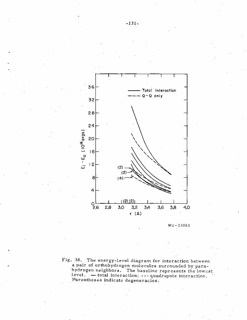
1/)

0' ... Q)

!f! 0

0 w

w

-131-

--- Total interaction ---Q-0 only

r (A)

MU-23063

Fig. 38. The energy-level diagram for interaction between a pair of orthohydrogen molecules surrounded by para­hydrogen neighbors. The baseline represents the lowest level. -total interaction; ---quadrupole interaction. " Parentheses indicate degeneracies.

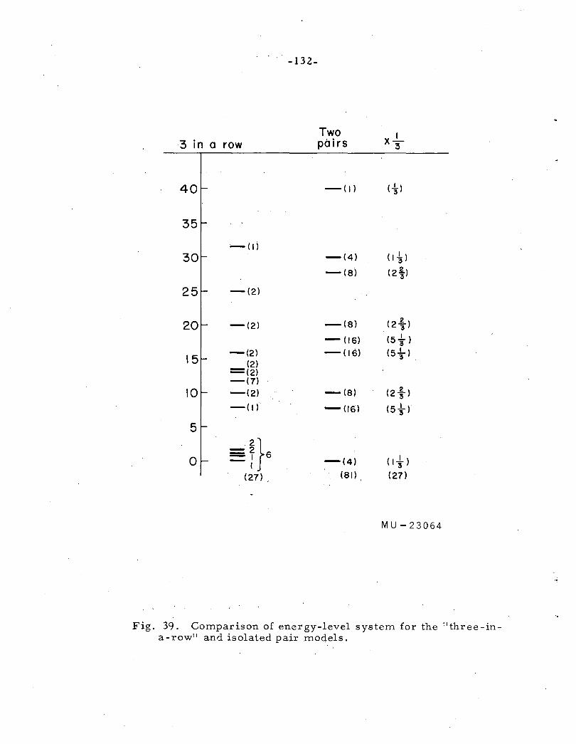
-132-

3 in a row

40

35

--<li

-(2)

-(2)

-(2)

(2) =(2) -(7)

-(2)

-(I)

5

0 Hs <27) '

Two pairs

-(I)

-(4)

-(8)

-(8)

-(16)

-(16)

-(8)

-(16)

-(4) (81)

x-' 3

(~)

(I~)

(2~)

(2 ~) (5t) (5.L)

3

(2 § ) (5 ~)

( I..!.. ) 3

(27)

MU-23064

Fig. 39. Comparison of energy-level system for the 11 three-in­a-row11 and isolated pair models.

..

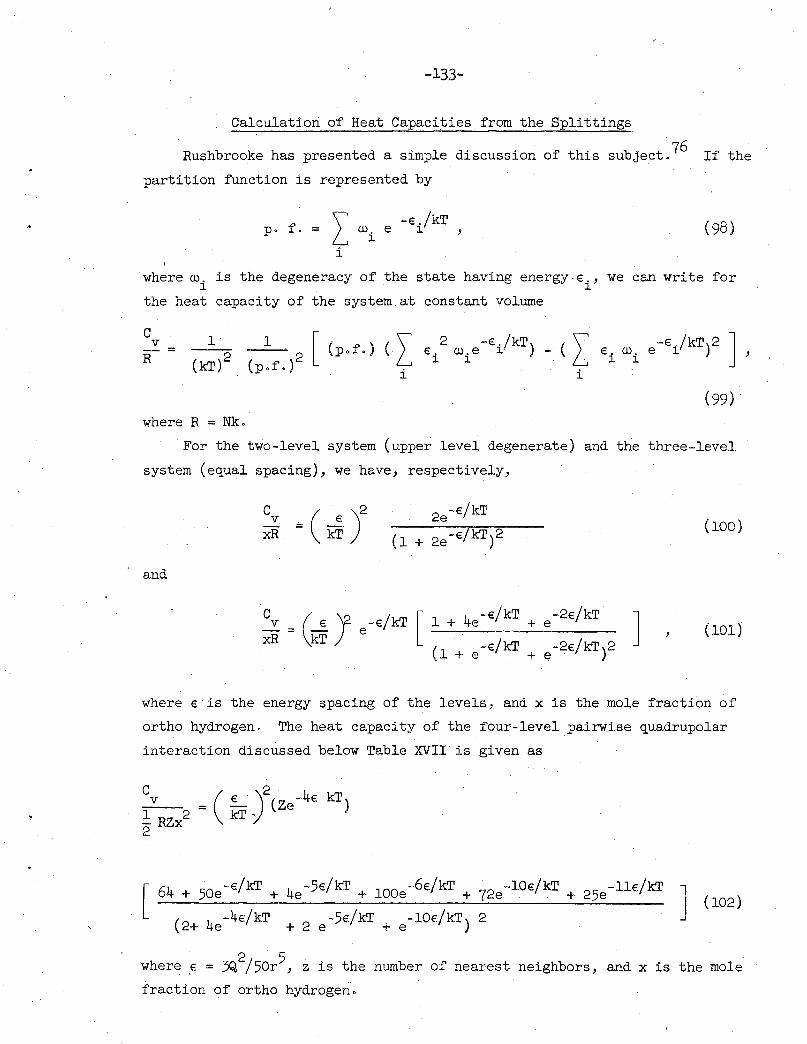
-133-

Calculation of Heat Capacities from the Splittings

Rushbrooke has presented a simple discussion of this subject.76 If the

partition function is represented by

\' -E ./kT p. f. = ~ roi e 1 , (98)

i

where ro. is the degeneracy of the state having energy-E., we can write for l l

the heat capacity of the system.at constant volume

c v

R 1 --

(kT)2

1 --2 (p.f.)

[ (p.f.) c I i

( L Ei roi e -Ei/kT)2 J ' i

(99)

where R = Nk.

For the two-level system (upper level degenerate) and the three-level

system (equal spacing), we have, respectively,

c ( )2 v . €

xR = kT 2e -E/kT

(100)

and

c . v ( € )2

xR ::::: kT [ 1 4 -€/kT -2E/kT + e + e

( 1 -E/kT -2E/kT)2 + e + e J (101)

where E is the energy spacing of the levels, and x is the mole fraction of

ortho hydrogen. The heat capacity of the four-level pairwise quadrupolar

interaction discussed below Table XVII. is given as

Cv ( E )2( -4€ kT) 1 2 = kT, · Ze - RZx 2

[ 64 + 5oe-€/kT + 4e-5•/kT + lOOe-6•/kT + 72e-lO</kT + 25e-ll•/kT J

( 2 4 -4E/kT 2 -5€/kT -10€/kT)· 2 + e + e + e

(102)

where € = 3Q2/50r5, z is the number of nearest neighbors, and x is the mole

fraction of ortho hydrogen·.

()

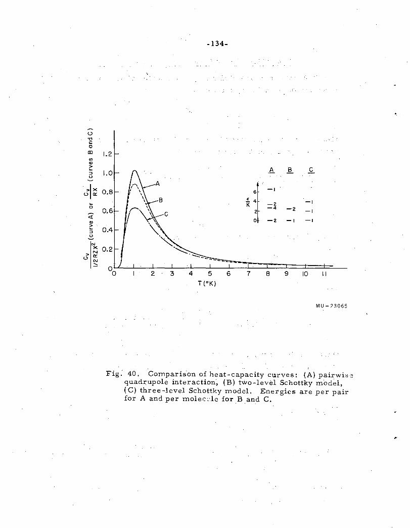
-c c: c IIl (/) C1)

> .... ::3 (.)

>IX u a::

.... 0

~

<t C1)

> .... ::3 (.)

N X > N

u a:: N .::::::

-134-

A B ~

*f -I

-2 -I -4 -2 -I

-2 -I -I

2 3 4 5 7 8 9 10 II

T (°K)

MU-23065

Fig. 40. Comparis.on of heat-capacity curves: (A) pairwis·c; quadrupole interaction·, (B) two-level Schottky model, (C) three-level Schottky model. Energies are per pair for A and per molec.'le for B and C.

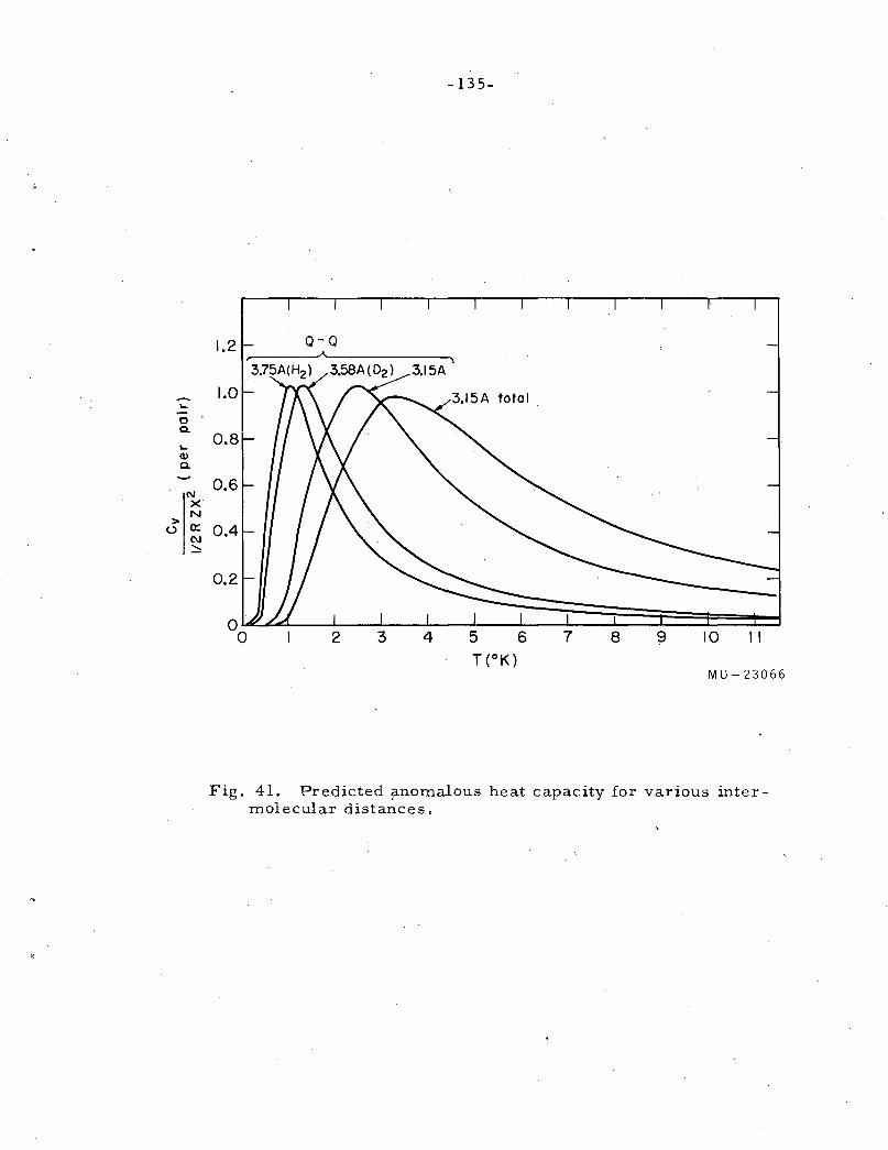
-.... c Q.

.... Q)

Q.

C\J X N

<5o:: C\1 ::::::

-135-

MU-23066

Fig. 41. Predicted f!.nomalous heat capacity for various inter­molecular distances.

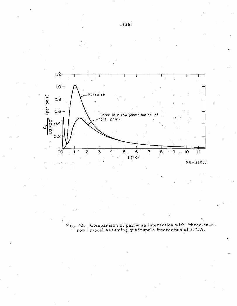
-.... 0 Q.

.... Q) Q.

N X N 0.4 >a::

0 C\1 .......

2

-136-

Three in a row (contribution of , one pair)

3 4 7 8 9 ' 10 II

MU-23067

Fig. 42. Comparison of pairwise interaction with 11 three-in-a­row11 model assuming quadrupole interaction at 3.75A.

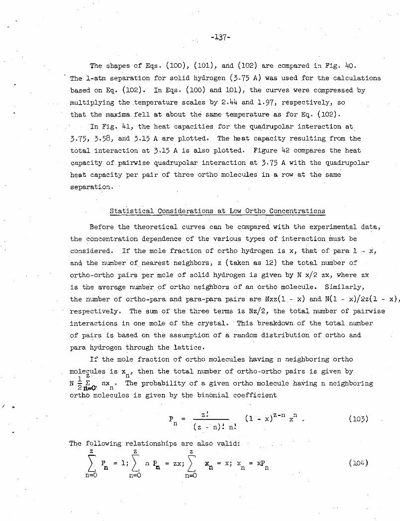
I .,..

-137-

The shapes of Eqs. (100), (101), and (102}are compared in Fig. 40.

The 1-atm separation for solid hydrogen (3.75 A) was used for the calculations

based on Eq. (102). In Eqs. (100) and 101), the curves were compressed by

multiplying the temperature scales by 2.44 and 1.97, respectively, so

that the maxima fell at about the same temperature as for Eq. (102).

In Fig. 41, the heat capacities for the quadrupolar interaction at

3.75, 3.58, and 3.15 A are plotted. The beat capacity resulting from the

total interaction at 3.15 A is also plotted. Figure 42 compares the heat

capacity of pairwise quadrupolar interaction at 3·75 A with the quadrupolar

heat capacity per pair of three ortho molecules in a row at the same

separation.

Statistical Considerations at Low Ortho Concentrations

Before the theoretical curves can be compared with the experiment~l data,

the concentration dependence of the various types of interaction must be

considered. If the mole fraction of ortho hydrogen is x, that of para 1 - x,

and the number of nearest neighbors, z (taken as 12) the total number of

ortho-ortho pairs per mole of solid hydrogen is given by N x/2 zx, where zx

is the average number of ortho neighbors of an ortho molecule. Similarly,

the number of ortho-para and para-para pairs are Nxz(l.- x) and N(l - x)/2z(l - x),

respectively. The sum of the three terms is Nz/2, the total number of pairwise

interactions in one mole of the crystal. · This breakdown of the total number

of pairs is based on the assumption of a random distribution of ortho and

para hydrogen through the lattice.

If the mole fraction of ortho molecules having n neighboring ortho

molegules is xn' then the total number of ortho-ortho pairs is given by

N ~ ~' nxn. The probability of a given ortho molecule having n neighboring

ortho molecules is given by the binomial coefficient

The following z

I p = n

n=O

z! p =

n ( z - n)! n!

relationships are also valid~ z z

1; ~ n Pn :::: ZXj ~ xn = Xj X

n=O n=O

(103)

= xP n n (104)

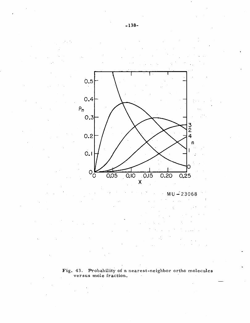
-138-

n

0.1

0.05 0.10 0.25

MU..:23068

Fig. 43. Probability of n nearest-neighbor ortho molecules versus mole fraction.

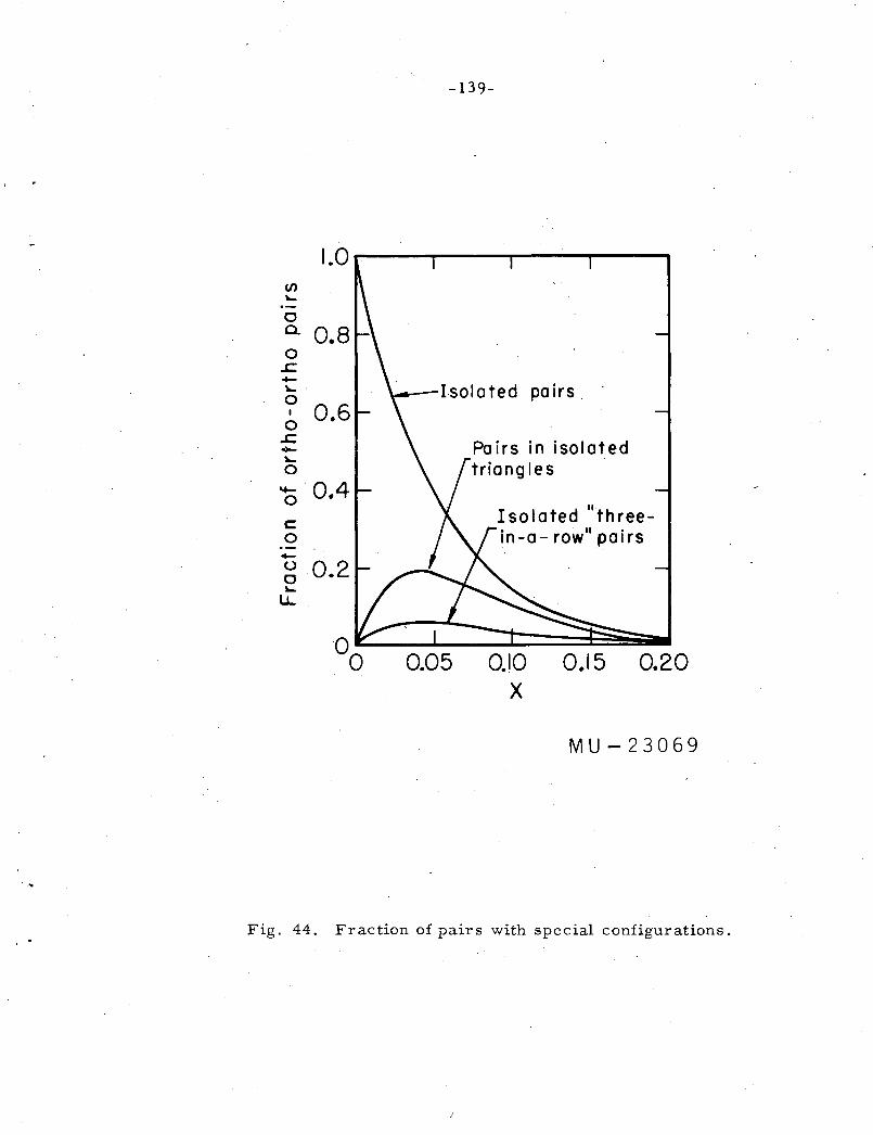
1.0 en .... 0 a. 0.8 0

.s::. -.... 0 0.6 I

0 .s::. -"-0 ~ 0.4 0

c 0 -(.) 0.2 0 ....

lJ...

0 0

-139-

~-I.solated pairs

0.05

Pairs in isolated triangles

Isolated 11three-

• II • 1n-a-row pa1rs

0.10 X

0.15 0.20

MU-23069

Fig. 44. Fraction of pairs with special configurations.

'

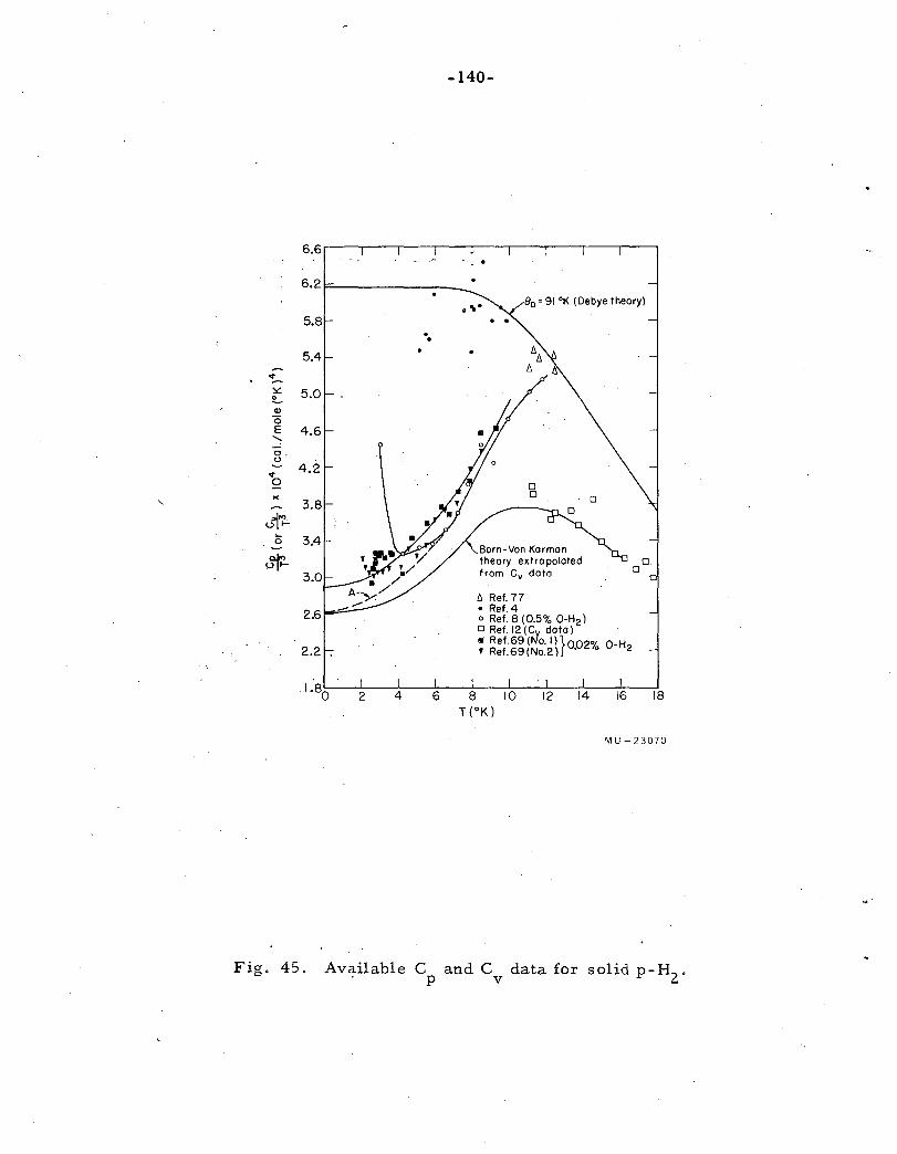
Q)

0 E ' o. (.)

<t 0

-140-

Born-Von Korman theory extra poloted from Cv data

f::. Ref. 77 • Ref. 4 o Ref. 8 ( 0.5% O-H2) o Ref. 12 (Cv dotal • Ret.69(No.ll}oo2 '% o-H2 ' Ref.69(No.2l · o

16 18

MU-23070

Fig. 45. Available Cp and Cv data for solid p-H2

.

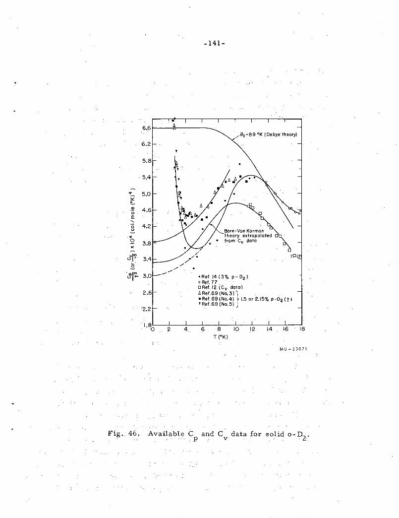
~ 0 E

' 0 (.)

¢

0 )(

8-t-. I"'

-141-

80 =89 "K (Debye theory)

Born-Von Korman theory extrapolated D

• from Cv doto

• Ref. 14 (3% p- D2l .o Ref. 77 . o Ref. 12 (Cv dote)

• Ref. 69 (No.4) 1.5 or 2.i5% p-02 (? l l1Ref.69(Nb.3l} , '

'Ref.69(No.5l . .

I. ~0· L.._.l.2-__.l4-.. _ _.~6--8L--I.LO~-.LI2----'-14----'.,-----'18

T (°K)

MU- 23071

Fig._ 46. Available Cp and Cvdata for solid o- D2

.

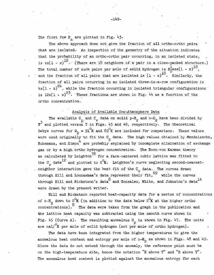
-142-

The first few P are plotted in Fig. 43. n

The above approach does not give the fraction of all ortho-ortho pairs

that are isolated. An inspection of the geometry of the situation indicates

that the probability of an ortho-ortho pair occurring, in an isolated state,

is zx(l- x)18 .: (There are 18 neighbors of a pair in a close-packed structure.)

The total number of such pairs per mole of solid hydrogen is N~xzx(l - x)18,

and the fraction of all pairs that are isolated is (1 - x)18

Similarly, the

fraction of all pairs occurring in an isolated three-in-a-row configuration is

4x(l - x) 24 , while the fraction occurring in i.solated triangular configurations

is 12x(l - x) 23. ·These fractions are shown in Fig. 44 as a function of the

ortho concentration.

Analysis of Available One-Atmosphere Data

The available CP, and Cv data on solid p-H2 and o-D2 have been divided by

T3 and plotted versus T in Figs. 45 and 46, respectively. The theoretical

Debye curves for QD = 91°K and 89°K are included for comparison. These values

were used originally to fit the C data. The high values obtained by Mendelssohn,

Ruhemann, and Simon 4 are probablyp explained by inpomplete elimination of exchange

gas or by a high ortho hydrogen concentration. The Born-von Karman theory 78 . as calculated by Leighton for a face-centered cubic lattice was fitted to

C. t. 12 OK the da a and plotted to 0 • v

Leighton's curve neglecting second-nearest-

neighbor interaction gave the best fit of the C data. The curves drawn

through Hill and Lounasinaa's data represent the~r fit, 69 while the curves

through Hill and Ricketson's data8 and Gonzalez, White, and Johnston's data14

were drawn by the present writer.

Hill and Ricketson reported heat-capacity data for a series of concentrations

of o-H2

down to 2°K (in addition to the data below 2°K at the higher ortho

concentrations).8 The data were taken from the graph in the publication and

the lattice heat capacity was subtracted using the smooth curve shown in

Fig. 45 (Curve A). The resulting anomalous C is shown in Fig. 47. The units p

are cal/°K per mole of solid hydrogen (not per mole of ortho hydrogen).

The data have been integrated from the higher temperatures to give the

anomalous heat content and entropy per mole of o-H2 as shown in Figs. 48 and 49.

Since the data do not extend through the anomaly, the reference point must be

on the high-temperature side, hence the notation "H above T11 and "s above T".

The anomalous heat content is plotted against the anomalous entropy f0r each

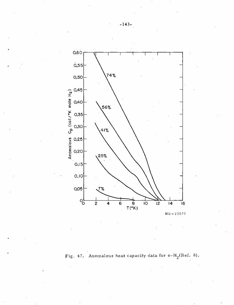
Q.)

0 E ~ 0 ........

0 E 0 c: <[

-143-

MU-23072

Fig. 47. Anomalous heat capacity data for o-H2(Ref. 8).

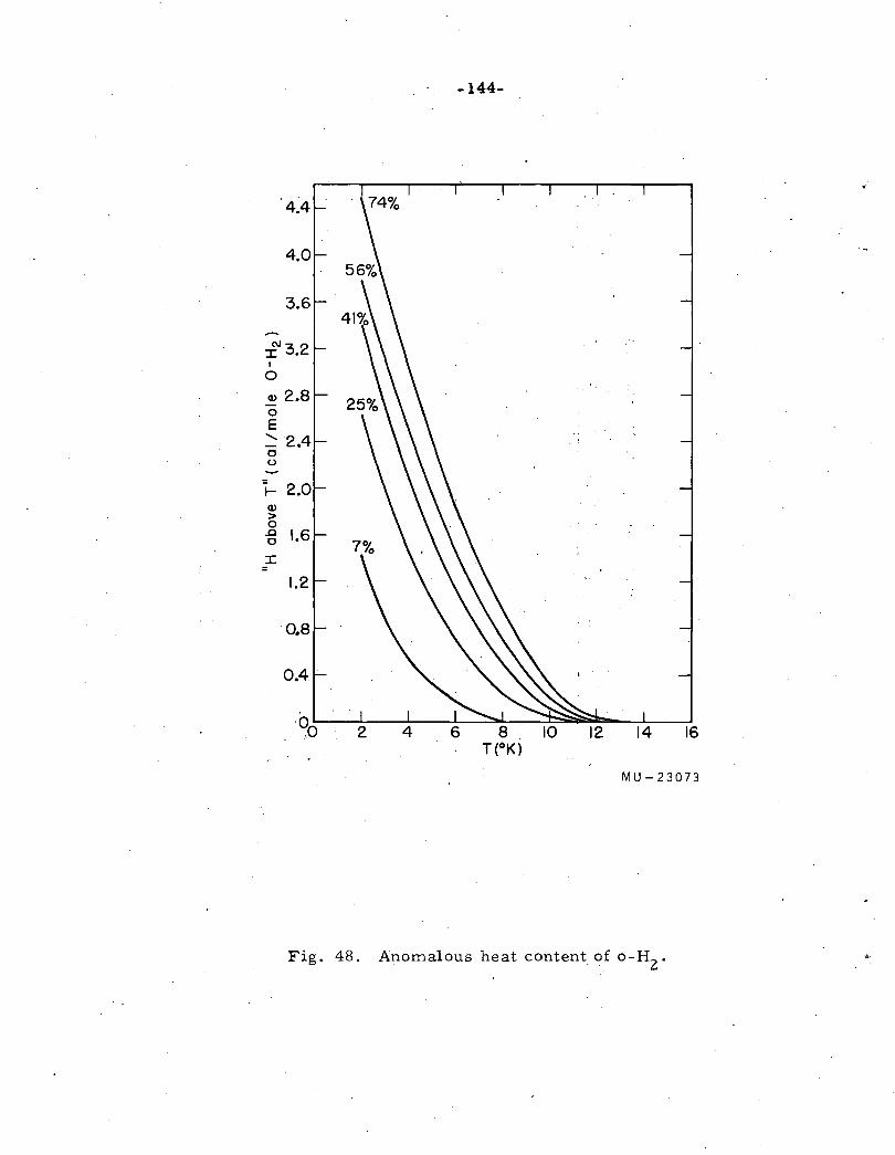
-144-

4.4

~3.2 I

0

Q) 2.8

-f-Q)

> 0 -§ 1.6

:r:

1.2

0.8

0.4

MU-23073

Fig. 48. Anomalous heat content of o-H2

.

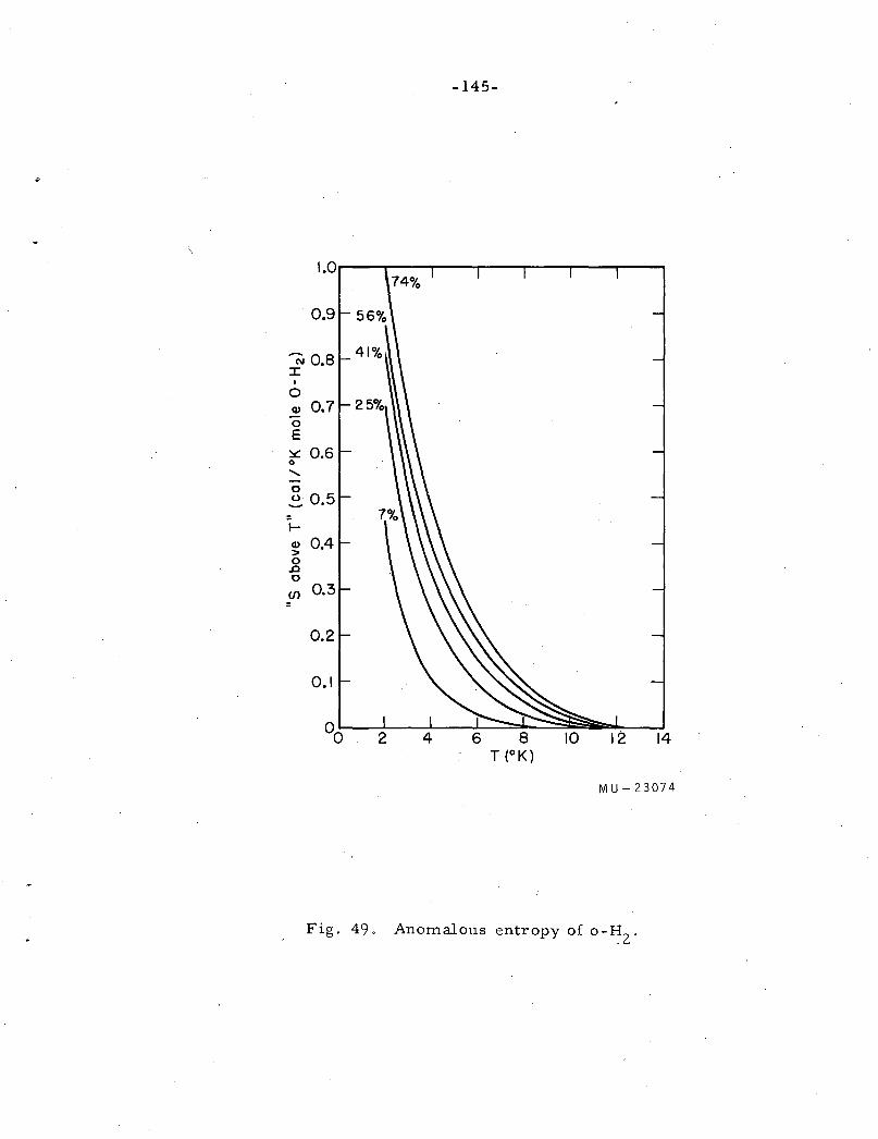
'N0.8 I

I

0 Q)

0 E ~ 0.6 0 ........

I-Q)

> 0 .0 0

CJ)

0.1

2

-145-

6 8 T (°K)

14

MU-23074

Fig. 49 0 Anomalous entropy of o-~2 o

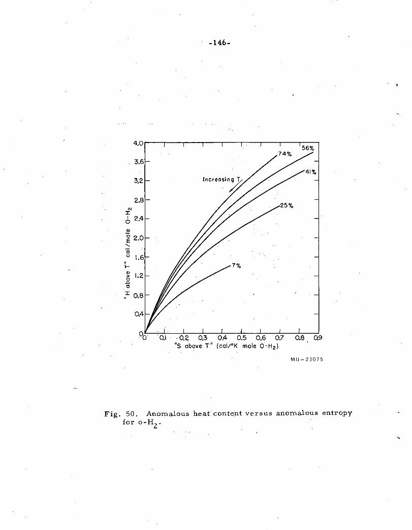
c 0

1-­Q)

~ .c c

. -146-

0.5 0.6 0.7 0.8 0.9

MU-23075

Fig. 50. Anomalous heat conte.nt versus anomalous entropy for o-H

2.

'•

-147-

concentration of o-H2 in Fig. 50. Temperature is a parameter on this plot,

increasing toward the origin. In order to compare the anomalous contributions

to the heat capacity with the theoretical expressions, Hill and Ricketson 1 s

7% and 0-5%data have been plotted in Fig. 51 and 52, respectively.8

The

data of Gonzalez et al on 3% o-D2 have been plotted in Fig. 53, 14 and Hill

and Lounasmaa's data on "nominal" o-D2 have been plotted in Fig. 54. 69 The

nominal p-D2

concentration of the latter data was 1.5% or 2.15%; depending

on whether the sample was equilibrated at the hydrogen boiling point or at

the deuterium triple point. Unfortunately, the authors did not r~port this

information.

For the 7% o-H2 case, it can be. seen from Fig. 43 that (1 - x)12

or

0.406 of the ortho molecules have all p-H2

nearest neighbors. Figure 44

indicates that of all the ortho-ortho pairs, (1- x)18 or 0.271 are wuisolated,u

i.e., completely surrounded by p-H2

nearest neighbors. If the molar heat

capa;ity of isolated o-H2 molecules is designated by Ca' that of isolated

pairs by Cb, and that of pairs in more complicated configurations by Cc'

the anomalous heat-capacity expression may be written

12 1 2 Cp = X (1 - X) Ca + ~ (12) X [

18 (1 - x) cb + (1 - x)

18} Cc J (105)

where x is the o-H2 mole fraction. If one assumes that Cc is given by the

"three-in-a-row" calculation, then the pairwise contributions may be calculated.

Since many other types of configuration appear besides the "three-in-a-row"

type, the above expression leads to some uncertainty in the theoretical

expression for cc. Thus the Cb and Cc contributions have been plotted

separately in Fig. 51 for the 7% o-H2 • The values of the theoretical curves

were obtained from Fig. 42. As was observed by Nakamura, 70 the theoretical

curves account for only one-half of the magnitude of the data. The residual

heat capacities were then fitted to the two and three-level anomalies described

in Eqs. (100) and (101) and plotted in Fig. 40. (The three-level model was

included merely because it was convenient and not for any theoretical reason.)

As may be seen from Fig. 51, both models can be fitted to the data by

adjusting the temperature scale. One then finds the splitting, e, given by -16 " '-16

3-59 x 10 ergs for the two-level model and by 2.61 x 10 ergs for the

three-level model. In order to obtain these numbers, Eq. (105) was used,

with the resulting assumption that the effect causing the splitting in the

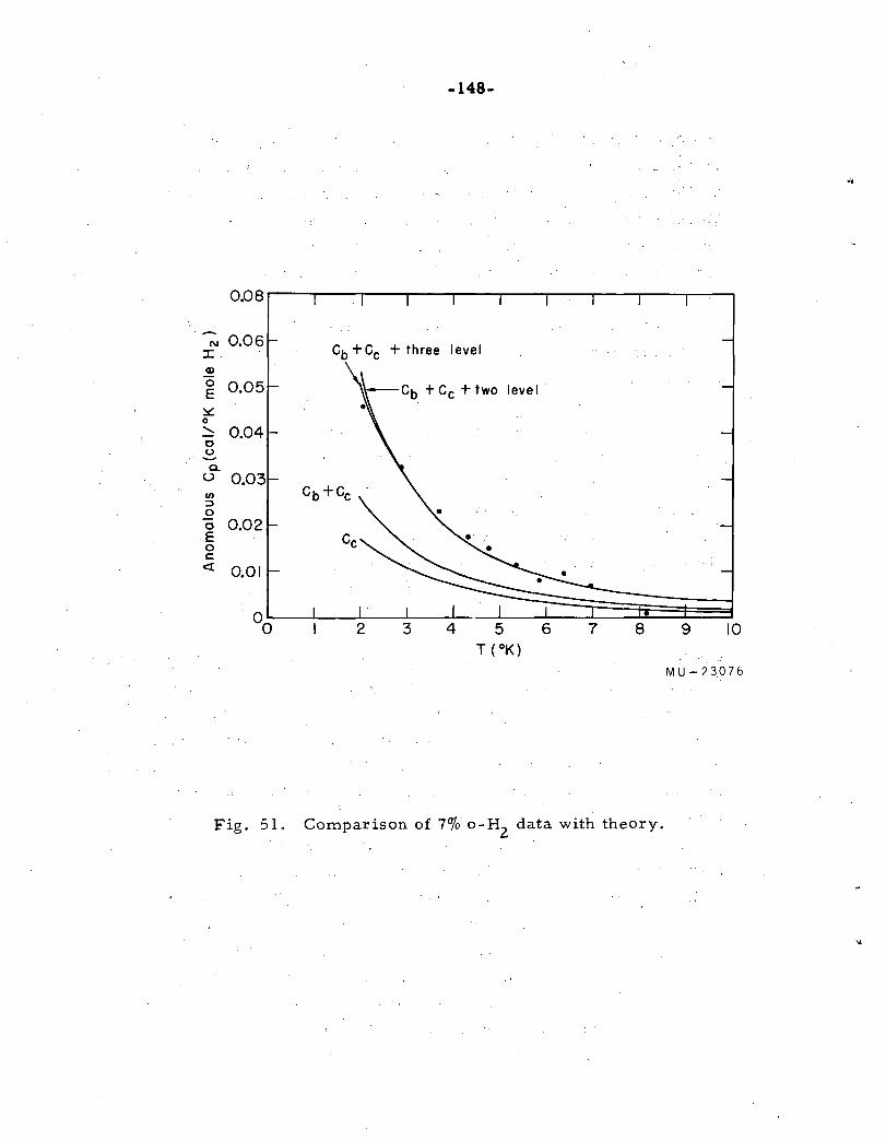
-148-

0.08

N :I: Cb + Cc + three level Q)

0 E ~ 0

' 0 0 -Q. (.)

1/)

::J 0

0 0.02 E 0 c: <t 0.01

00 8 9 10

MU-23.076

Fig. 51. Comparison of 7o/o o-H2

data with theory.

,)

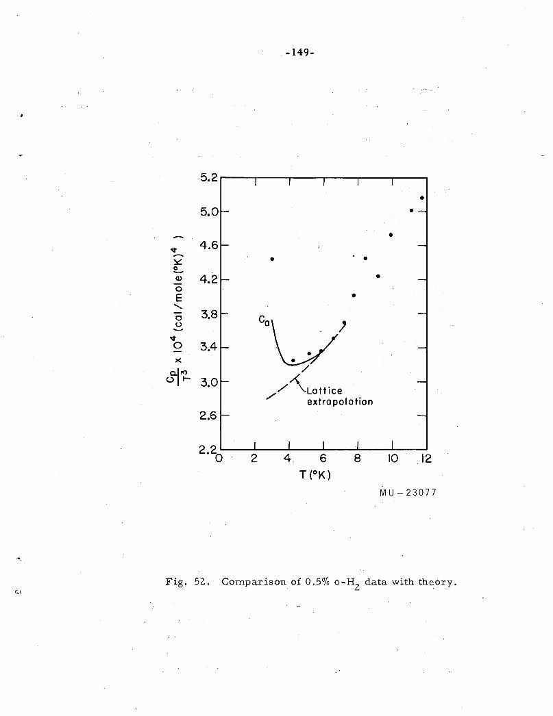
-149-

. -~ .

5.2

• •

• v - • • • ~ 0 -Q) • -0 E • ' -0 GaVJ (,)

v 0 3.4 )(

~~~ / u 1- /~Lattice

/ extrapolation

2.6

2.20 2 4, 6 8 10 12 T (°K)

MU-23077

Fig. 52. Comparison of 0.5o/o o-H2

data with theory.

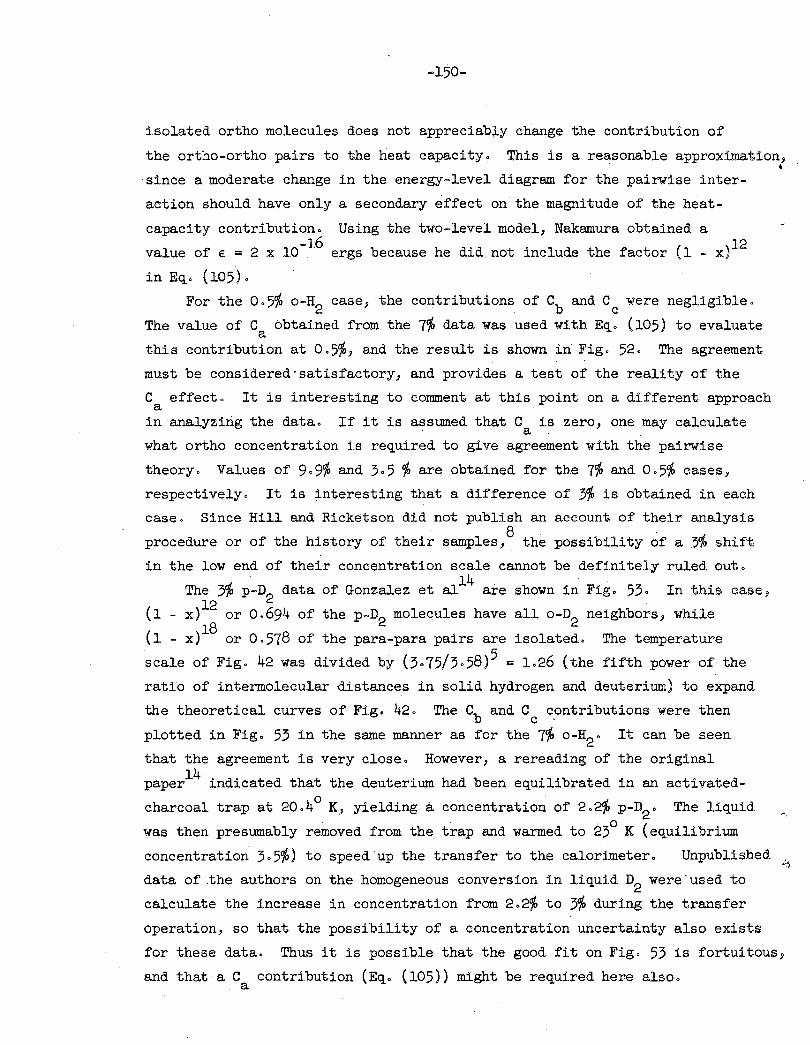
-150-

isolated ortho molecules does not appreciab~y change the contribution of

the ortho-ortho pairs to the heat capacity. This is a re~sonable approximation~

since a moderate change in the energy-level diagram for the pairwise inter-

action should have only a secondary effect on the magnitude of the heat­

capacity contribution. Using the two-level model, Nakamura obtained a

value of € = 2 x 10-16 ergs because he did. not include the factor (1 - x)12

in Eq. (105).

For the 0.5'{o o-H2 case, the contributions of Cb and Cc were negligible.

The value of Ca obtained from the 7% data was used with Eq. (105) to evaluate

this contribution at 0.5%, and the result is shown in Fig. 52. The agreement

must be considered·satisfactory, and provides a test of the reality of the

C effect. a

It is interesting to comment at this point on a different approach

in analyzing the data. If it is assumed that C is zero, one may calculate . a . what ortho concentration is required to give agreement with the pairwise

theory. Values of 9·9% and 3.5 % are obtained for the 7% and 0.5% cases,

respectively. It is interesting that a difference of 3% is obtained in each

case. Since Hill and Ricketson did not publish an account of their analysis

procedure or of the history of their samples,8

the possibility of a 3% shift

in the low end of their concentration scale cannot be definitely ruled out.

The 3% p-D2 data of Gonzalez et a114

are shown in Fig. 53· In this case, 12

(1 - x) or 0.694 of the p-D2 molecules have all o-D2 neighbors, while

(1 - x)18

or 0.578 of the para-para pairs are isolated. The temperature

scale of Fig. 42 was divided by (3.75/3.58) 5 = 1.26 (the fifth power of the

ratio of intermolecular distances in solid hydrogen and deuterium) to expand

the theoretical curves of Fig. 42. The Cb and C contributions were then c . plotted in Fig. 53 in the same manner as for the 7% o-H2 • It can be seen

that the agreement is very close. However, a rereading of the original

paper14 indicated that the deuterium had been equilibrated in an activated­

charcoal trap at 20.4° K, yielding a concentration of 2.2% p-D2 • The liquid

was then presumably removed from the trap and warmed to 23° K (equilibrium

concentration 3·5%) to speed up the transfer to the calorimeter. Unpublished

data of .the authors on the homogeneous conversion in liquid D2 were·used to

calculate the increase in concentration from 2.2'{o to 3% during the transfer

'

,.,

. .:,

operation, so that the possibility of a concentration uncertainty also exists

for these data. Thus it is possible that the good fit on Fig. 53 is fortuitousJ

and that a C contribution (Eq. (105)) might be required here also. a

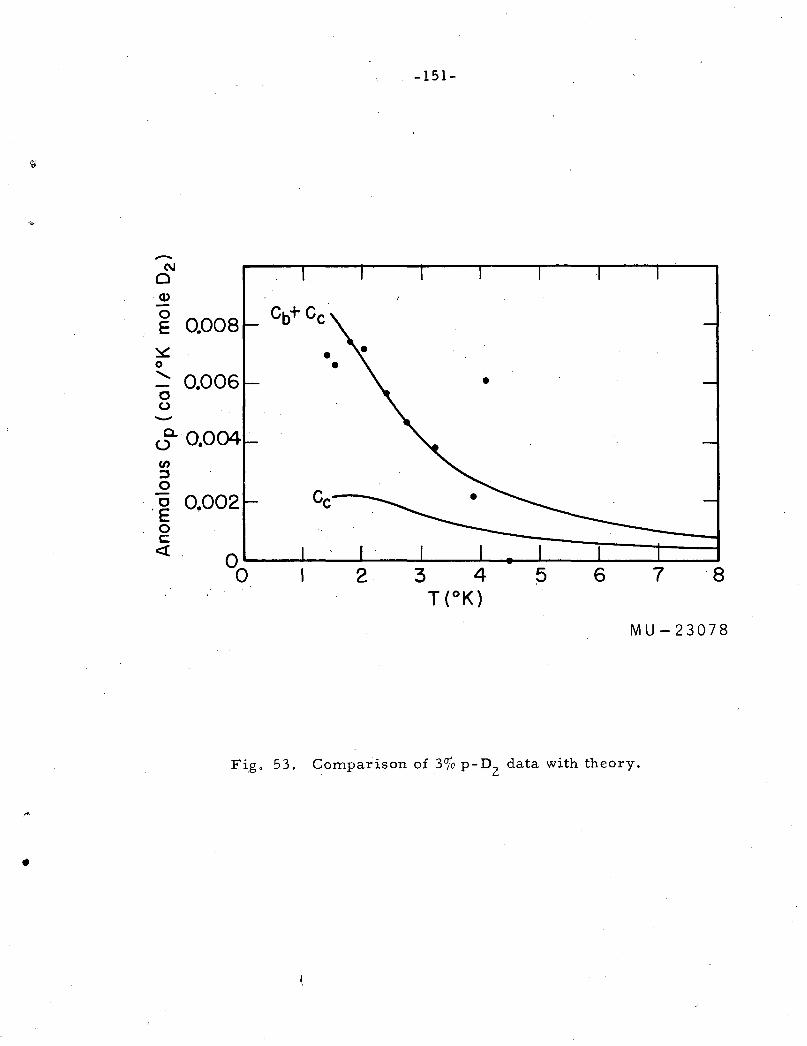
-151-

.,.

-C\1 0 Q)

0 0.008 E

~ 0

' 0.006 0 (.) -en ::J 0 0 0.002 ·e 0 c::: <(

00 2 3 4 0 6 7 8 T {°K)

MU- 23078

Fig, 53. Comparison of 3o/o p-D2

data with theory .

•

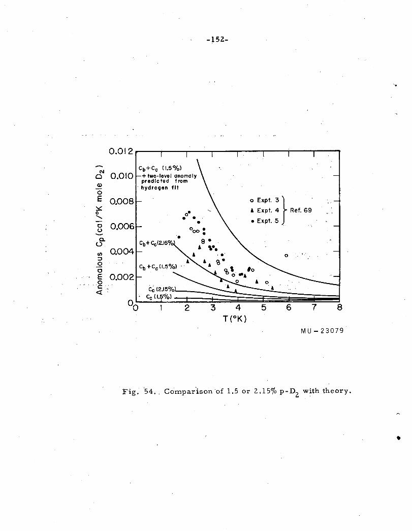
-(\1

0 Q)

0 E ~ 0 .........

0 (.)

Q. (.)

f/)

:::J 0 0 E 0 c: <!

0.010 cb + Cc (1.5 %>

+two-level anomaly predicted from hydrogen fit

-152-

o Expt 3 } · • Expt. 4 Ref. 69

• Expt. 5 .. .·

Fig. '54 .. Compar.ison ·of 1.5 or 2.15o/o p-D2 with theory.

•

-153-

69 The data of Hill and Lounasmaa on 1. 5% or 2 .15% p-D2 are shown in

Fig. 54. The theoretical Cb and Cc contributions are shown for both

contributions. The C contribution predicted by the hydrogen data is a .

also plotted for 1.5% p-D2 • If the Ca effect is due to translational

effects in the lattice as suggested by Nakamura, 70 one might expect the

effect to be smaller for deuterium than for hydrogen. . .

The above analysis of the data onthe o-H2, and p-D2 anomalyat low

concentration indicates that there probably is a term iri the heat capacity

proportional to the concentration, although more precise and more carefully

defined data would make the conclusion more certain. It seems likely

that part of the splitting of the levels of isolated ortho molecules is

caused by second-nearest-neighbor effects, and this phenomenon should be

considered when comparing the data with theories based on translational

effects.

Comment on London's Theory

London29 suggested that 11 the initial work of compression in solid

hydr,ogen is mainly used to reduce space for the molecules by confining

their rotational motion to a smaller angle rather than to drive the

molecules deeper into their mutual Vander Waals repulsion fieid. 1129 On

this basis he reasoned that "quenching11 of the rotational motion should

occur when the energy supplied by compression was at least sufficient to

raise the ground state (J = 0) to the level of the first excited state

(J = 1). This corresponds to 340 cal/mole for H2 and 170 cal/mole for D2 •

The pressures necessary to supply such an energy of compression were

estimated to be 5500 and 4000 kg/cm2

for H2 and D2 , respectively.

The above reasoning seems inconsistent with the work of Hobbs16 on

th~ zero-point energy of H2

, HD, and D2 (which, incidentally, was

suggested by London). A casual observation of the curves in Hobbs paper

indicates that between 1 and 5000 kg/cm2, the potential energy of solid

hydrogen decreases about 100 cal/mole, while the zero-point energy rises

400 to 500 cal/mole, giving a net energy increase of about 300 cal/mole.

Thus it would be more correct to say that between 1 and 5000 kg/cm2, the

energy of compression only increases the zero-point energy of the lattice.

London's estimate of the pressure necessary to 11 quench" the rotation still

seems valid, however, because above 5000 kg/cm2

, the repulsive potential

energy rises vepy steeply.

-154-

ACKNOWLEOOMENTS

The author is grateful to Professor Kenneth s. Pitzer for his many

timely suggestions and for his understanding and patient guidance during

the course of this work~

The author is also indebted to Professor N. E. Phillips for many

illuminating discussions .on low-temperature calorimetric technique.

It is a pleasure to acknowledge the collaboration of Mr. R. s. Hickman

of the Lawrence Radiation Laboratory Mechanical Engineering Department on

the design of the high-pressure system and the mechanical design of the

calorimeter. The expert and efficient aid of Mr. E. c. Miner of the

Radiation Laboratory Mechanical Engineering Department in the design and

construction of many of the necessary components of the apparatus greatly

expedited the progress of the project.

The enthusiastic cooperation of Mr. J. Beuneman of the Chemistry

Department Shop was indispensible in assembling and improving the apparatus.

'The assistance of Mr. H. Wandesf6rd of the 'Accelerator Technician Shop is

also to be acknowledged. Aid in secretarial matters was eX'cellently provided

by Mrs. Jane Waite.

The author also wishes to acknowledge the collaboration of Mr. Gunter

Ahlers and a conversation with Mr. L. · V. Gregor.

The author is indebted to the Bell Telephone Laboratories and the

National Science Foundation for· predoctoral fellowships during 1958-59 and 1959~60, respectively, and to the United States Atomic Energy Commission

for other support of this project.

"'

'•'

-l55-

APPENDICES

A. Assembly and Disassembly .of the Calorimeter

The following comments should be of use in further work on the calorimeter,

since there is a certain sequence of operations that should be followed in

taking it apart and putting it together if damage is to be avoided. The pro­

cedure is as follows:

1. Remove the vacuum ·can bottom by Un.bol:ting the flange at D.

2. Remove the copper radiation baffle at DD and unglue the thermocouple from

the bottom of the liquid-nitrogen shield; then unbolt the shield and drop

it into the vacuum can.

3. The vacuum can and liquid-nitrogen-shield bottoms may then be lifted out

of the pressure shield.

4. Unglue the thermocouple on the outer bath shield, unbolt it at Q, and

remove, being careful not to damage the wires underneath it.

5. Unsolder and unbolt the front half of the isothermal shield for access

to the cell.

6. To remove the cell f"rom the calorimeter, simply disconnect it and pull

it out with the capillaries through flange Y ..

7• If it is desired to raise the inner and outer bath, or the liquid-nitrogen

reservoir, the cell must be disconnected from these parts and can be

clamped to the flange of the vacuum can.

8. Disconnect the vacuum and vapor pressure lines at the top, and using

the eyebolts, raise flanges B and C together and hoist several inches

so thatthe top of the liquid-nitrogen shield,can be pulled out.

9. Lower the flanges and then·rl3-ise C by itself .. This operation requires

two people -- one hoisting and the other guiding the assembly to avoid

damaging the wires.

10. Assembling the calorimeter is simply the reverse of the above operations.

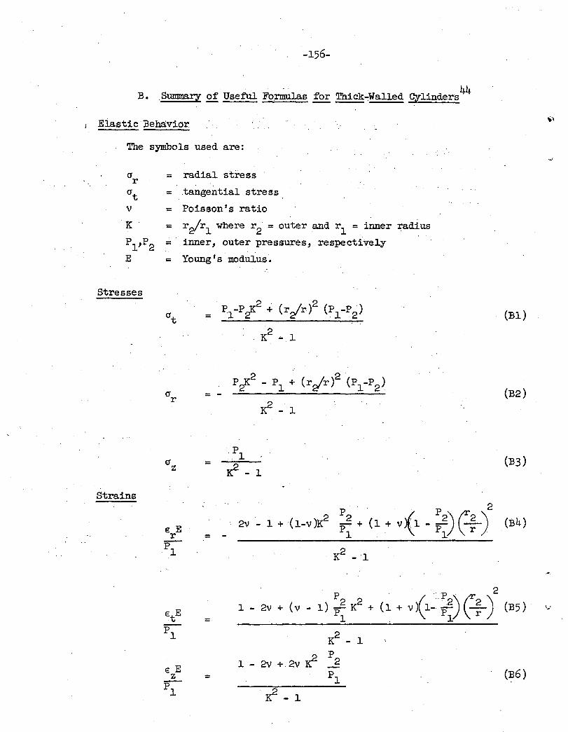
-156-

B. .Summary of Useful Formulas for Thick~Walled Cylinders 44

Elastic Behavior

The symbols used are:

cr = radial stress r crt = .tangential stress.

v = Poisson's ratio

K = r~r1 where r 2 = outer and r 1 = inner radius

P1

,P2 = inner, outer pressures, respectively

E = Young's modulus.

Stresses

= -P2K2 - pl + (r~r)2 (Pl-P2)

~- l

(Bl)

(B2)

'"'

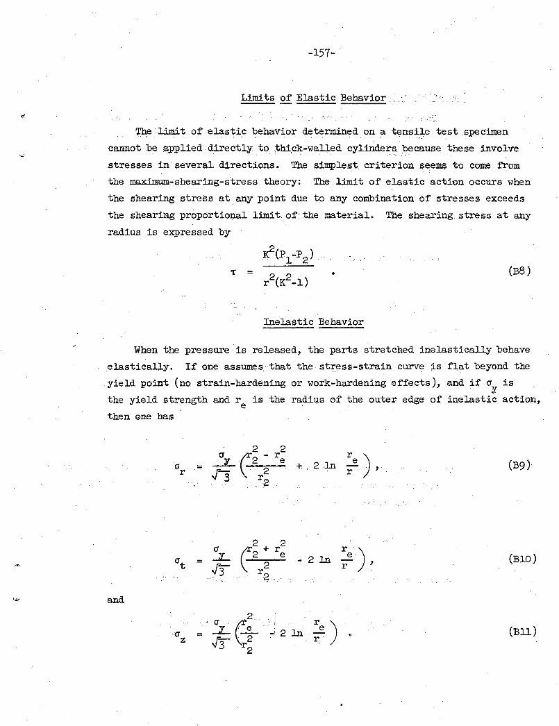
(.c;:l

-157-

Limits of Elastic Behavior . ·:,__ \

.·. J:···

'+he limit of. elastic behavior determined on a tensi~e test specimen

cannot .be applied directly to .thi.ck-wa1led cylinde;r~ _1;>ecause. these involve

stresses in several directions. The simplest criterion seems to come from

the maximum...;shearing-stress theory: The limit of elastic action occurs when

the shearing stress at any point due to any combination of stresses exceeds

the shearing proportio~al limit of· the material. The shearing stress at any

radius is expressed by

• (B8)

Inelastic Behavior

When the pressure is released, the parts stretched inelastically behave

elastically. If on~ assumes. that the stress-strain curve is flat beyond the

yield point (no strain-hardening or work-hardening effects), and if cr is y

the yield strength and r is the radius of the outer edge of inelastic action, e then one has

+ 2 ln :e) , . (B9)

2 2 cr t2:

r :e), ...L e 2ln (BlO) crt = -

J"3 r2.

and

'lt_; :! ... re ) cr = _: 2 ln 0 (Bll)

z J"3 ·r~ r··

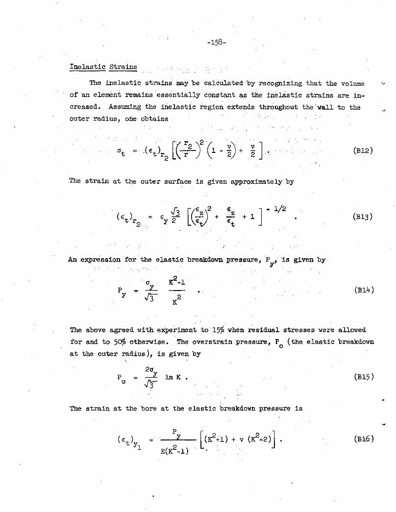
-158-

Inelastic Strains

The inelastic strains may be calculated by recognizing that the volume

of an element remains essentiallY constant as the iniHastic strains are in­

creased. Assuming the iri.elast:i.c· region extends throughout the'vtall to the

outer radius, one obtains

The strain at the outer surface is given approximately by

+ 1 J - 1/2

An expression :for the elastic breakdown pJ;"essure, P , is given by y

.. a K2-1· p = ..L

y .f3 2 K

. .

(Bl2)

(Bl3)

(Bl4)

The above agreed· with experiment to 15% when residual stresses were allowed

for and to 5rf/o otherwise. The overstrain pressure, P (the elastic breakdown 0

at the outer radius), is given by

p 0

2a = _x lnK.

.f3

The strain at the bore at the elastic breakdown pressure is

·-....!Opy~- [~~+1) + v (~-2)] •

E(K2-l) ·

(Bl5)

(Bl6)

....

...

-159-

REFERENCES

L. W. H.Keeson, .J., DeSmedt, and H. H. Mooy, Communs. Phys. Lab• Univ.

Leiden 209d (1930) •

2. v. s. Kogan, B. G. Lazarev, and R. F. Bulatova, Soviet.Phys. JETP _!:t, 593 (1957).

3· v. S. Kogan, B. G. Lazarev, and R. F. Bulatova, Soviet Phys. JETP 1' 165 (1958 ).

4. K. Mendelssolm, M. Ruhemann, and F. Simon, z. physik .. Chern. (Leipzig)

Bl5, 121 (1931).

5. L. Pauling, Phys. Rev. 36, 430 (1930).

6. F. Simon, Ergeb. exakt. Naturw. 21 260, 269 (1930).

7. K. Schaefer, z. physik. Chern. (Leipzig) B42, 380 (1939 ).

8. R. W. Hill and B. W. A. Ricketson,-Phil. Mag. 45, 277 (1954).

9. R. W. Hill and B. W. A. Ricketson, and F. Simon, Conf. de Phys .. des

Basses Temp. (Simonet Cie., Paris 1955), No. 76, p. 317.

10. K. Tomita, Proc. Pbys. Soc. (London) A68, 214 (1955).

11. K. Clusius and E. Bartholome, z. physik. Chem. (Leipzig) B30 1 237 (1935 ).

12. E. Bartholome and A. Eucken, z. ,Elektrochem. 42, 547 (1936 ).

13• H. D .. Megaw, Philo Mag. 28, 129 (1939).

14. 0. D. Gonzalez, D. White, and H. L. Johnston, J. Phys .. Chern., 61, 773

(1957 ).

15. F. London, Proc. Roy. Soc. (London) Al53, 576 (193?)•

16. M. Hobbs, J. Chern. Phys. 1, 318 (1939).

17. E. Cremer and M. Polanyi, z. physik. Chern. (Leipzig) B2l, 459 (1933).

18. E. Cremer, z. physik •. Chern. (Leipzig) B391 445 (1938).

19. E. Cremer, z. physik. Chern. (Leipzig) B28, 199 (1935 ).

20. B. V. Rollin and E. W:atson, Conf. de Phys. des Basses Temp. (Simon et

Cie., 1955) No. 63.

21. M. Bloom; Physica 23, 767 (1957).

22. G. W• Smith and c. F. Squire, Phys. Rev. lll, 188 (1958).

23. K. Motizuki and T. Nagamiya, J. Phys. Soc. Japan ll, 93 (1956).

24. K. Motizuki, J. Phys. Soc. Japan 12, 163 (1957).

25. F. Reif and E. M. Purcell, Phys. Rev. _2!, 631 (1953).

26. F. Simon, Nature 133, 529 (1934).

27. J. A. Stewart, Pbys .. Rev., 971 578 (1955) ..

-160-

28. J. A. Stewart, J. Phys~ Chem. Solids ! 1 146 (1956).

29. Fe London, Physo Rev. 102, 168 (1956).

30. K. s. Pitzer:, Quantum Chemistry (Prentice-Hall,· Inc., New York 1953)

p. 327.

31 •. J. deBoer,.Physica 2,-363 (1942)~

32. W •. D. McCormick and W. M., Fairbank, BulL Am. Phys. Soc~ [2) J., 166

(1958 ).

33. Re Berman, J. Appl. Phys. 27, 318 (1956)o

34., J .. R. Clement and E. H.-Quinnell, Rev. Sci .. Instr. 23, 213 (1952).

35. J. R. Cleme11t~ E. H. QuinnE'lll, M. C .. Steele, R. A. Rein,- and R. L.

Solecek, Rev. Sci .. Instr. ·. 24, 545 (1953 ).

36. R. Berman·, Rev. Scio Instr. 25, 94 (1954). 37. J. S. Dugdale and F. E. Siinon, Proc. Roy .. Soc. (London) A21.8, 291

(1953 ). 38. P. W .. Bridgman, The Physics of. High Pressure (G .• Bell. ·and Sons,

London, 1958 ), p. lj{)6. ._, ..

39. o. L. Anderson, Some Safety Problems Associated With High Pressure

Equipment. Obtained from Mr •. D. H. Newhall of the. Ha.rwo.od.

Engineering Co., ·Walpole, Mass.

4o. W. Paul and D .. M. WarshaUer, Rev, Sci. Instr. 27, 418 (1956).,

4L W. Paul, G. B.; ·Benedek; and D .. Mo Warshauer, Rev .. Sci. Instr. 30, 874

(1959 ). 42. K. So' Pitzer, Dept. of Chemistry, University of California, Berkeley,

unpublished tables.

43. c. A. swenson, Phys. Rev • .22,, 423 (1955) •

. 44. E. W. Comings, High. Pressure Technology,. Chapter 6 (McGraw-Rill Book

Co., New York,. N. Y., 1956)... - .

45. Private -communication :from Professor G. Benedek of Harvard University

August 1960.

46. D. H. Weitzel and O. E. Park; Rev. Sci. Instr. 27, 57 (1956).

47. D. H. Weitzel, W .. ·v. Loebenstein, J. W •. Draper, and o. E. Park,

J. Research Nat~ Blir. Standards 6o, 221 (1958). 48. M. Konecnikp Laboratory Note; NBS ·cryogenic Engineering Laboratory,

Project No. 8123:~ File-No. 59:..8, J"u.ly 2, 1959· 49. C. M. Cunningham, D. S. 'Ch8.pin,··and H._L. Johnston,· J. Am. Chem. Soc.

80, 2382 (1958 ). . . .

50. D. S. Chapin and H. L. Johnston, J. Am. ·Chem. Soc. 79, 24o6 (1957).

'-'

..

-161-

51. E. H. Kennard, Kinetic Theory of Gases (McGraw-Hill Book Co., New York,

1938) Chapter IV pp. 162-5, 180-4.

52. J. 0. Hirschfelder, C. F. Curtiss, and R. B. Bird, Holecular Theory of

Liguids and Gases (John Wiley and Sons, Inc., New York, 1954)

Chapters 7 and 8.

53· A. Farkas, Orthohydrogen, Parahydrogen, and Heavy Hydrogen (Cambridge

University Press, Cambridge 1935).

54. E. R. Grilly, Rev~ Sci. Instr. 24, 72 (1953).

55. H. W. Woolley, R. B. Scott, and F. G. Brickwedde, J. Research Nat. Bur.

Standards 41, 379 ( 1948).

56. H. Van Duk and H. Durieux, Helium Vapor Pressure Scale T155

, K. Onnes

Laboratory, Leiden.

57. W. DeSorbo and G. E. Nichols, J. Phys. Chern. Solids§, 352 (1958).

58. J. R. Clement, presented at lOth Annual Calorimetry Conference, General

Electric Research Laboratory, Schenectady, Ne-v1 York (Sept. 1954).

59· Nat. Bur. Standards (u.s.) Ann. Rept. Circ. 556.

60. American Institute of Physics Handbook (McGraw-Hill Book Co., New York

1957 ).

61. R. B. Scott, Cryogenic Engineering (D. Van Nostrand Co., 1959).

62. F. B. Hildebrand, Advanced Calculus for Engineers (Prentice-Hall, Inc.,

New York, 1948 ) •

63. M. Hichels, w. de Graff, T. Wassenaar, J. H. Levelt, P. Louwerse,

Physica 25, 25 (1959).

64. H. 1. Johnston and D. White, Trans. ASME, 785 (August 1950).

65. F. E. Simon, M. Ruhemann, andW. A. H. Ed1vards, Z. physik. Chern. B6, 331

( 1930 ).

66.

67.

68 •

R. L. Hills and E. R. Grilly, Phys. Rev. lOl, 1246 (1956).

C. Bartholome, Z. physik. Chern. B33, 387 (1936). ~-

Private communication from·L. B. Nesbitt and M. D. Fiske, General Electric

Co., Schenectady, N. Y., Jan. l7, 1959.

69. R. W. Hill and 0. V. Lounasmaa, Phil. Mag. ~' 785 (1959 ).

70. T. Nakamura, Prog. Theoret. Phys. (Kyoto) 14, 135 (1955).

71. T. Nakamura and N. Uryu, Busseiron Kenku 96, 49 (1956).

72. J. Ha.rrick and N. F. Ramsey, Physo Rev. 88, 228 (l952).

73. F. London, J. Phys. Chern. 46, 305 (1942).

74. See, for example, L. I. Schiff, Quanturn Hechanics (HcG:t>a-vr-Hill Book Co.,

Nev1 York, 1955).

I

75. J. A. Stratton, Electromagnetic Theory (McGraw-Hill Book Co., New York,

1941.

76. G. s. Rushbrooke, Introduction to Statistical M:e~hanics (Oxford at the.

Clarendon Press, Lpn{iqn, 1949 ).

77" .K. Clusius and K. ·Hiller, z. physik~ ahem. (Leipzig) ·B4, 158 (1929).

78. R. B. Leighton, Revs. Mod. Phys. :20., 165 (191R3 ).

79. E. C. Kerr., E. ·B.· Rifkin, H. L. Johnston, and J. T.· Clarke, J" Am.. Chem.

Soc. ]J, 282 (1951) ..

•

/

This report was prepared as an account of Government sponsored work" Neither the United States, nor the Com­m1ss1on, nor any person acting on behalf of the C6mmission:

A" Makes any warranty or representation, expressed or implied, with respect to th·e accuracy, completeness, or usefulness of the information contained in this report, or that the us~ of any information, appa­ratus, method, or process disclosed in this report may not infringe privately owned rights; or

B" Assumes any liabilities with respect to the use of, or for damages resulting from the use of any infor­mation, apparatus, method, or process disclosed in this report"

As used in the above, "person acting on behalf of the Commission" includes any employee or contractor of the Com­mission, or employee of such contractor, to the extent that such employee or contractor of the Commission, or employee of such contractor prepares, disseminates, or provides access to, any information pursuant to his employment or contract with the Commission, or his employment with such contractor"