clustering multivariate normal distributions

Clustering Multivariate Normal Distributions

Frank Nielsen1,2 and Richard Nock3

1 LIX — Ecole Polytechnique, Palaiseau, [email protected]

2 Sony Computer Science Laboratories Inc., Tokyo, [email protected]

3Ceregmia — Universite Antilles-Guyane, Schoelcher, France

[email protected]

Abstract. In this paper, we consider the task of clustering multivari-ate normal distributions with respect to the relative entropy into a pre-scribed number, k, of clusters using a generalization of Lloyd’s k-meansalgorithm [1]. We revisit this information-theoretic clustering problemunder the auspices of mixed-type Bregman divergences, and show thatthe approach of Davis and Dhillon [2] (NIPS*06) can also be deriveddirectly, by applying the Bregman k-means algorithm, once the propervector/matrix Legendre transformations are defined. We further explainthe dualistic structure of the sided k-means clustering, and present anovel k-means algorithm for clustering with respect to the symmetricalrelative entropy, the J-divergence. Our approach extends to differentialentropic clustering of arbitrary members of the same exponential familiesin statistics.

1 Introduction

In this paper, we consider the problem of clustering multivariate normal distri-butions into a given number of clusters. This clustering problem occurs in manyreal-world settings where each datum point is naturally represented by multipleobservation samples defining a mean and a variance-covariance matrix modelingthe underlying distribution: Namely, a multivariate normal (Gaussian) distribu-tion. This setting allows one to conveniently deal with anisotropic noisy datasets, where each point is characterized by an individual Gaussian distributionrepresenting locally the amount of noise. Clustering “raw” normal data sets isalso an important algorithmic issue in computer vision and sound processing. Forexample, Myrvoll and Soong [3] consider this task for adapting hidden Markovmodel (HMM) parameters in a structured maximum a posteriori linear regres-sion (SMAPLR), and obtained improved speech recognition rate. In computervision, Gaussian mixture models (GMMs) abound from statistical image mod-eling learnt by the expectation-maximization (EM) soft clustering technique [4],and therefore represent a versatile source of raw Gaussian data sets to manip-ulate efficiently. The closest prior work to this paper is the differential entropicclustering of multivariate Gaussians of Davis and Dhillon [2], that can be derivedfrom our framework as a special case.

F. Nielsen (Ed.): ETVC 2008, LNCS 5416, pp. 164–174, 2009.c© Springer-Verlag Berlin Heidelberg 2009

Clustering Multivariate Normal Distributions 165

A central question for clustering is to define the appropriate information-theoretic measure between any pair of multivariate normal distribution objectsas the Euclidean distance falls short in that context. Let N(m, S) denote1 thed-variate normal distribution with mean m and variance-covariance matrix S.Its probability density function (pdf.) is given as follows [5]:

p(x; m, S) =1

(2π)d2√

detSexp

(− (x − m)T S−1(x − m)

2

), (1)

where m ∈ Rd is called the mean, and S � 0 is a positive semi-definite ma-

trix called the variance-covariance matrix, satisfying xT Sx ≥ 0 ∀x ∈ Rd. The

variance-covariance matrix S = [Si,j ]i,j with Si,j = E[(X(i)−m(i))(X(j)−m(j))]and mi = E[X(i)] ∀i ∈ {1, ..., d}, is an invertible symmetric matrix with posi-tive determinant: detS > 0. A normal distribution “statistical object” can thusbe interpreted as a “compound point” Λ = (m, S) in D = d(d+3)

2 dimensionsby stacking the mean vector m with the d(d+1)

2 coefficients of the symmetricvariance-covariance matrix S. This encoding may be interpreted as a serial-ization or linearization operation. A fundamental distance between statisticaldistributions that finds deep roots in information theory [6] is the relative en-tropy, also called the Kullback-Leibler divergence or information discriminationmeasure. The oriented distance is asymmetric (ie., KL(p||q) �= KL(q||p)) anddefined as:

KL(p(x; mi, Si)||p(x; mj , Sj)) =∫

x∈Rd

p(x; mi, Si) logp(x; mi, Si)p(x; mj , Sj)

dx. (2)

The Kullback-Leibler divergence expresses the differential relative entropywith the cross-entropy as follows:

KL(p(x;mi, Si)p(x;mj , Sj)) = −H(p(x;mi, Si))−∫

x∈Rd

p(x;mi, Si) log p(x;mj , Sj)dx,

(3)

where the Shannon’ differential entropy is

H(p(x; mi, Si)) = −∫

x∈Rd

p(x; mi, Si) log p(x; mi, Si)dx, (4)

independent of the mean vector:

H(p(x; mi, Si)) =d

2+

12

log(2π)ddetSi. (5)

Fastidious integral computations yield the well-known Kullback-Leibler diver-gence formula for multivariate normal distributions:1 We do not use the conventional (μ, Σ) notations to avoid misleading formula later

on, such as∑n

i=1 Σi, etc.

166 F. Nielsen and R. Nock

KL(p(x; mi, Si)||p(x; mj , Sj)) =12

log |S−1i Sj |+

12tr

((S−1

i Sj)−1) − d

2+

12(mi − mj)T S−1

j (mi − mj), (6)

where tr(S) is the trace of square matrix S, the sum of its diagonal elements:tr(S) =

∑di=1 Si,i. In particular, the Kullback-Leibler divergence of normal

distributions reduces to the quadratic distance for unit spherical Gaussians:KL(p(x; mi, I)||p(x; mj , I)) = 1

2 ||mi − mj ||2, where I denotes the d × d iden-tity matrix.

2 Viewing Kullback-Leibler Divergence as a Mixed-TypeBregman Divergence

It turns out that a neat generalization of both statistical distributions andinformation-theoretic divergences brings a simple way to find out the same resultof Eq. 6 by bypassing the integral computation. Indeed, the well-known normaldensity function can be expressed into the canonical form of exponential familiesin statistics [7]. Exponential families include many familiar distributions suchas Poisson, Bernoulli, Beta, Gamma, and normal distributions. Yet exponentialfamilies do not cover the full spectrum of usual distributions either, as they donot contain the uniform nor Cauchy distributions.

Let us first consider univariate normal distributions N(m, s2) with associatedprobability density function:

p(x; m, s2) =1

s√

2πexp −

((x − m)2

2s2

). (7)

The pdf can be mathematically rewritten to fit the canonical decompositionof distributions belonging to the exponential families [7], as follows:

p(x; m, s2) = p(x; θ = (θ1, θ2)) = exp {< θ, t(x) > −F (θ) + C(x)} , (8)

where θ = (θ1 = μσ2 , θ2 = − 1

2σ2 ) are the natural parameters associated with the

sufficient statistics t(x) = (x, x2). The log normalizer F (θ) = − θ21

4θ2+ 1

2 log −πθ2

is astrictly convex and differentiable function that specifies uniquely the exponentialfamily, and the function C(x) is the carrier measure. See [7,8] for more detailsand plenty of examples. Once this canonical decomposition is figured out, we cansimply apply the generic equivalence theorem [9] [8] Kullback-Leibler↔Bregmandivergence [10]:

KL(p(x; mi, Si)||p(x; mj , Sj)) = DF (θj ||θi), (9)

to get the closed-form formula easily. In other words, this theorem (see [8] for aproof) states that the Kullback-Leibler divergence of two distributions of the sameexponential family is equivalent to the Bregman divergence for the log normalizergenerator by swapping arguments. The Bregman divergence [10] DF is defined asthe tail of a Taylor expansion for a strictly convex and differentiable function F as:

DF (θj ||θi) = F (θj) − F (θi)− < θj − θi, ∇F (θi) >, (10)


where < ·, · > denote the vector inner product (< p, q >= pT q) and ∇F is thegradient operator. For multivariate normals, the same kind of decompositionexists but on mixed-type vector/matrix parameters, as we shall describe next.

3 Clustering with Respect to the Kullback-LeiblerDivergence

3.1 Bregman/Kullback-Leibler Hard k-Means

Banerjee et al. [9] generalized Lloyd’s k-means hard clustering technique [1]to the broad family of Bregman divergences DF . The Bregman hard k-meansclustering of a point set P = {p1, ..., pn} works as follows:

1. Initialization. Let C1, ..., Ck be the initial k cluster centers called the seeds.Seeds can be initialized in many various ways and is an important step toconsider in practice, as explained in [11]. The simplest technique, calledForgy’s initialization [12], is to allocate at random seeds from the sourcepoints.

2. Repeat until converge or stopping criterion is met(a) Assignment. Associate to each “point” pi its closest center with respect

to divergence DF : pi → arg minCj∈{C1,...,Ck} DF (pi||Cj). Let Cl denotethe lth cluster, the set of points closer to center Cl than to any othercluster center. The clusters form a partition of the point set P . Thispartition may be geometrically interpreted as the underlying partitionemanating from the Bregman Voronoi diagram of the cluster centersC1, ..., Ck themselves, see [8].

(b) Center re-estimation. Choose the new cluster centers Ci ∀i ∈ {1, ..., k}as the cluster respective centroids: Ci = 1

|Ci|∑

pj∈Cipj. A key property

emphasized in [9] is that the Bregman centroid defined as the minimizerof the right-side intracluster average arg minc∈Rd

∑pi∈Cl| DF (pi||c) is in-

dependent of the considered Bregman generator F , and always coincidewith the center of mass.

The Bregman hard clustering enjoys the same convergence property as thetraditional k-means. That is, the Bregman loss function

∑kl=1

∑pi∈Cl

DF (pi||Cl)monotonically decreases until convergence is reached. Thus a stopping criterioncan also be choosen to terminate the loop as soon as the difference between theBregman losses of two successive iterations goes below a prescribed threshold.In fact, Lloyd’s algorithm [1] is a Bregman hard clustering for the quadraticBregman divergence (F (x) =

∑di=1 x2

i ) with associated (Bregman) quadraticloss. As mentioned above, the centers of clusters are found as right-type sumaverage minimization problems. For a n-point set P = {p1, ..., pn}, the center isdefined as

arg minc∈Rd

DF (pi||c) =1n

n∑i=1

pi. (11)


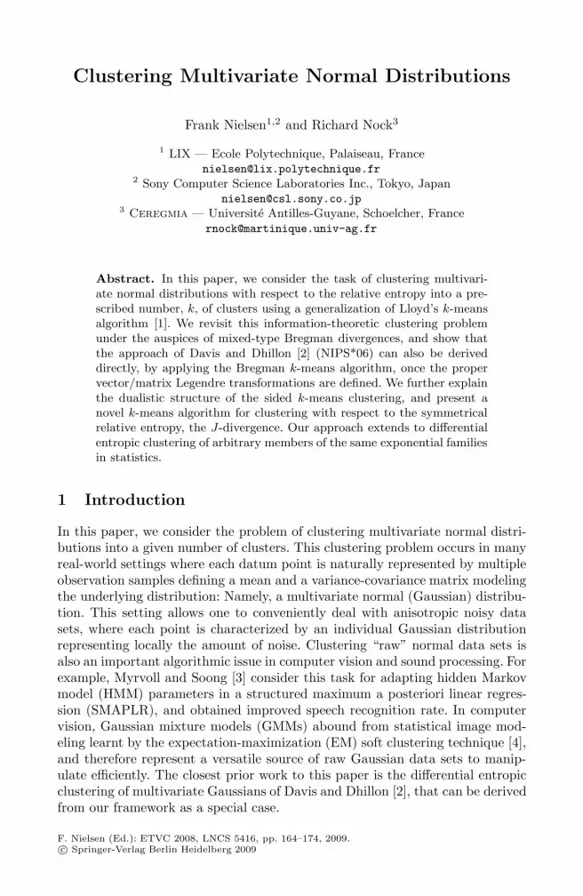
Fig. 1. Bivariate normal k-means clustering (k = 3, d = 2, D = 5) with respect tothe right-type Bregman centroid (the center of mass of natural parameters, equivalentto the left-type Kullback-Leibler centroid) of 32 bivariate normals. Each cluster isdisplayed with its own color, and the centroids are rasterized as red variance-covarianceellipses centered on their means.

That is, the Bregman right-centroid is surprisingly invariant to the consideredBregman divergence [9] and always equal to the center of mass. Note that al-though the squared Euclidean distance is a Bregman (symmetric) divergence, itis not the case for the single Euclidean distance for which the minimum averagedistance optimization problem yields the Fermat-Weber point [13] that does notadmit closed-form solution.

Thus for clustering normals with respect to the Kullback-Leibler divergenceusing this Bregman hard clustering, we need to consider the oriented distanceDF (θi||ωl) for the log normalizer of the normal distributions interpreted as mem-bers of a given exponential family, where ωl denote the cluster centroid in thenatural parameter space. Since DF (θi||ωl) = KL(cl||pi) it turns out that the hardBregman clustering minimizes the Kullback-Leibler loss

∑kl=1

∑pi∈Cl

KL(cl||pi).We now describe the primitives required to apply the Bregman k-means clus-tering to the case of the Kullback-Leibler clustering of multivariate normaldistributions.

3.2 Mixed-Type Parameters of Multivariate Normals

The density function of multivariate normals of Eq. 1 can be rewritten intothe canonical decomposition of Eq. 8 to yield an exponential family of orderD = d(d+3)

2 (the mean vector and the positive definite matrix S−1 accounting


respectively for d and d(d+1)2 parameters). The sufficient statistics is stacked onto

a two-part D-dimensional vector/matrix entity

x = (x, −12xxT ) (12)

associated with the natural parameter

Θ = (θ, Θ) = (S−1m,12S−1). (13)

Accordingly, the source parameter are denoted by Λ = (m, S). The log normal-izer specifying the exponential family is (see [14]):

F (Θ) =14Tr(Θ−1θθT ) − 1

2log detΘ +

d

2log 2π. (14)

To compute the Kullback-Leibler divergence of two normal distributions Np =N (μp, Σp) and Nq = N (μq , Σq), we use the Bregman divergence as follows:

KL(Np||Nq) = DF (Θq||Θp) (15)

= F (Θq) − F (Θp)− < (Θq − Θp), ∇F (Θp) > . (16)

The inner product < Θp, Θq > is a composite inner product obtained as the sumof two inner products of vectors and matrices:

< Θp, Θq >=< Θp, Θq > + < θp, θq > . (17)

For matrices, the inner product < Θp, Θq > is defined by the trace of the matrixproduct ΘpΘ

Tq :

< Θp, Θq >= Tr(ΘpΘTq ). (18)

Figure 1 displays the Bregman k-means clustering result on a set of 32 bivari-ate normals.

4 Dual Bregman Divergence

We introduce the Legendre transformation to interpret dually the former k-means Bregman clustering. We refer to [8] for detailed explanations that weconcisely summarize here as follows: Any Bregman generator function F admitsa dual Bregman generator function G = F ∗ via the Legendre transformation

G(y) = supx∈X

{< y, x > −F (x)}. (19)

The supremum is reached at the unique point where the gradient of G(x) =<y, x > −F (x) vanishes, that is when y = ∇F (x). Writing X ′

F for the gradientspace {x′ = ∇F (x)|x ∈ X}, the convex conjugate G = F ∗ of F is the functionX ′

F ⊂ Rd → R defined by

F ∗(x′) =< x, x′ > −F (x). (20)


Primal (natural Θ) Dual (expectation H)

Fig. 2. Clustering in the primal (natural) space Θ is dually equivalent to clustering inthe dual (expectation) space H . The transformations are reversible. Both normal datasets are visualized in the source parameter space Λ.

It follows from Legendre transformation that any Bregman divergence DF ad-mits a dual Bregman divergence DF ∗ related to DF as follows:

DF (p||q) = F (p) + F ∗(∇F (q))− < p, ∇F (q) >, (21)= F (p) + F ∗(q′)− < p, q′ >, (22)= DF ∗(q′||p′). (23)

Yoshizawa and Tanabe [14] carried out non-trivial computations that yieldthe dual natural/expectation coordinate systems arising from the canonical de-composition of the density function p(x; m, S):

H =(

η = μH = −(Σ + μμT )

)⇐⇒ Λ =

(λ = μΛ = Σ

), (24)

Λ =(

λ = μΛ = Σ

)⇐⇒ Θ =

(θ = Σ−1μΘ = 1

2Σ−1

)(25)

The strictly convex and differentiable dual Bregman generator functions (ie.,potential functions in information geometry) are F (Θ) = 1

4Tr(Θ−1θθT ) − 12 log

detΘ + d2 log π, and F ∗(H) = − 1

2 log(1+ ηT H−1η) − 12 log det(−H)− d

2 log(2πe)defined respectively both on the topologically open space R

d × C−d , where Cd

denote the d-dimensional cone of symmetric positive definite matrices. The H ⇔Θ coordinate transformations obtained from the Legendre transformation aregiven by

H = ∇ΘF (Θ) =(

∇ΘF (θ)∇ΘF (Θ)

)=

( 12Θ−1θ

− 12Θ−1 − 1

4 (Θ−1θ)(Θ−1θ)T

)(26)

=(

μ−(Σ + μμT )

)(27)


and

Θ = ∇HF ∗(H) =(

∇HF ∗(η)∇HF ∗(H)

)=

(−(H + ηηT )−1η− 1

2 (H + ηηT )−1

)=

(Σ−1μ12Σ−1

). (28)

These formula simplify significantly when we restrict ourselves to diagonal-only variance-covariance matrices Si, spherical Gaussians Si = siI, or univariatenormals N (mi, s

2i ).

5 Left-Sided and Right-Sided Clusterings

The former Bregman k-means clustering makes use of the right-side of the di-vergence for clustering. It is therefore equivalent to the left-side clustering forthe dual Bregman divergence on the gradient point set (see Figure 2). The left-side Kullback-Leibler clustering of members of the same exponential family isa right-side Bregman clustering for the log normalizer. Similarly, the right-sideKullback-Leibler clustering of members of the same exponential family is a left-side Bregman clustering for the log normalizer, that is itself equivalent to aright-side Bregman clustering for the dual convex conjugate F∗ obtained fromLegendre transformation.

We find that the left-side Bregman clustering (ie., right-side Kullback-Leibler)is exactly the clustering algorithm reported in [2]. In particular, the cluster centersfor the right-side Kullback-Leibler divergence are left-side Bregman centroids thathave been shown to be generalized means [15], given as (for (∇F )−1 = ∇F ∗ ):

Θ = (∇F )−1

(n∑

i=1

∇F (Θi)

). (29)

After calculus, it follows in accordance with [2] that

S∗ =

(1n

∑i

S−1i

)−1

, (30)

m∗ = S∗(n∑

i=1

1n

S−1i mi). (31)

6 Inferring Multivariate Normal Distributions

As mentioned in the introduction, in many real-world settings each datum pointcan be sampled several times yielding multiple observations assumed to be drawnfrom an underlying distribution. This modeling is convenient for consideringindividual noise characteristics. In many cases, we may also assume Gaussiansampling or Gaussian noise, see [2] for concrete examples in sensor data net-work and statistical debugging applications. The problem is then to infer fromobservations x1, ..., xs the parameters m and S. It turns out that the maxi-mum likelihood estimator (MLE) of exponential families is the centroid of the


sufficient statistics evaluated on the observations [7]. Since multivariate normaldistributions belongs to the exponential families with statistics (x, − 1

2xxT ), itfollows from the maximum likelihood estimator that

μ =1s

s∑i=1

xi, (32)

and

S =

(12s

s∑i=1

xixTi

)− μμT . (33)

This estimator may be biased [5].

7 Symmetric Clustering with the J-Divergence

The symmetrical Kullback-Leibler divergence 12 (KL(p||q)+KL(q||p)) is called the

J-divergence. Although centroids for the left-side and right-side Kullback-Leiblerdivergence admit elegant closed-form solutions as generalized means [15], it is alsoknown that the symmetrized Kullback-Leibler centroid of discrete distributionsdoes not admit such a closed-form solution [16]. Nevertheless, the centroid ofsymmetrized Bregman divergence has been exactly geometrically characterizedas the intersection of the geodesic linking the left- and right-sided centroids(say, cF

L and cFR respectively) with the mixed-type bisector: MF (cF

R, cFL) = {x ∈

X | DF (cFR||x) = DF (x||cF

L )}. We summarize the geodesic-walk approximationheuristic of [15] as follows: We initially consider λ ∈ [λm = 0, λM = 1] and repeatthe following steps until λM −λm ≤ ε, for ε > 0 a prescribed precision threshold:

1. Geodesic walk. Compute interval midpoint λh = λm+λM

2 and correspond-ing geodesic point

qh = (∇F )−1((1 − λh)∇F (cFR) + λh∇F (cF

L )), (34)

Fig. 3. The left-(red) and right-sided (blue) Kullback-Leibler centroids, and the sym-metrized Kullback-Leibler J-divergence centroid (green) for a set of eight bivariatenormals


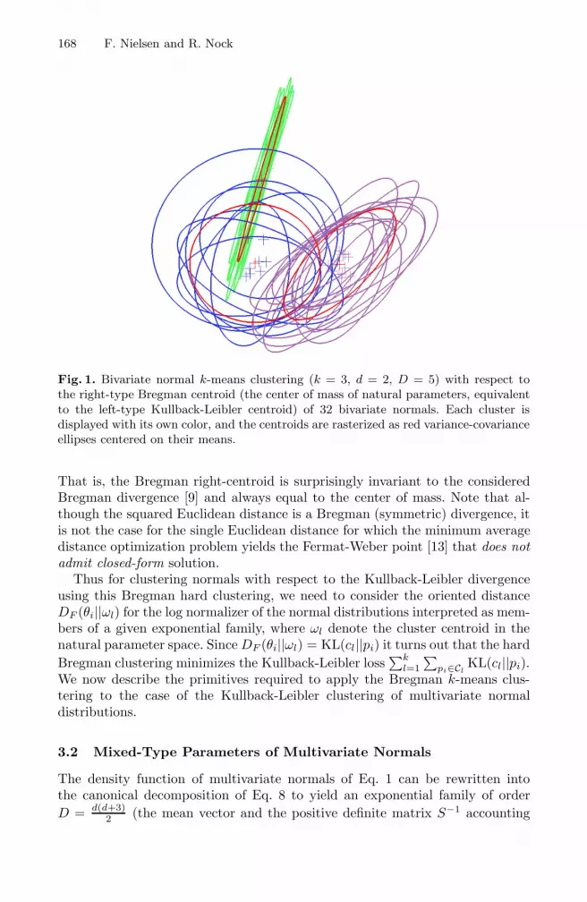
Fig. 4. Clustering sided or symmetrized multivariate normals. For identical variance-covariance matrices, this Bregman clustering amounts to the regular k-means. Indeed,in this case the Kullback-Leibler becomes proportional to the squared Euclidean dis-tance. See demo applet at http://www.sonycsl.co.jp/person/nielsen/KMj/

2. Mixed-type bisector side. Evaluate the sign of DF (cFR||qh)−DF (qh||cR

L),and

3. Dichotomy. Branch on [λh, λM ] if the sign is negative, or on [λm, λh]otherwise.

Figure 3 shows the two sided left- and right-sided centroids, and the sym-metrized centroid for the case of bivariate normals (handled as points in 5D).We can then apply the classical k-means algorithm on these symmetrized cen-troids. Figure 4 displays that the multivariate clustering applet, which shows theproperty that it becomes the regular k-means if we fix all variance-covariancematrices to identity. See also the recent work of Teboulle [17] that further gen-eralizes center-based clustering to Bregman and Csiszar f -divergences.

8 Concluding Remarks

We have presented the k-means hard clustering techniques [1] for clustering mul-tivariate normals in arbitrary dimensions with respect to the Kullback-Leiblerdivergence. Our approach relies on instantiating the generic Bregman hard clus-tering of Banerjee et al. [9] by using the fact that the relative entropy betweenany two normal distributions can be derived from the corresponding mixed-typeBregman divergence obtained by setting the Bregman generator as the log nor-malizer function of the normal exponential family. This in turn yields a dualinterpretation of the right-sided k-means clustering as a left-sided k-means clus-tering that was formerly studied by Davis and Dhillon [2] using an ad-hoc opti-mization technique. Furthermore, based on the very recent work on symmetricalBregman centroids [15], we showed how to cluster multivariate normals with re-spect to the symmetrical Kullback-Leibler divergence, called the J-divergence.

http://www.sonycsl.co.jp/person/nielsen/KMj/


This is all the more important for applications that require to handle symmetricinformation-theoretic measures [3].

References

1. Lloyd, S.P.: Least squares quantization in PCM. IEEE Transactions on InformationTheory 28(2), 129–136 (1982); first published in 1957 in a Technical Note of BellLaboratories

2. Davis, J.V., Dhillon, I.S.: Differential entropic clustering of multivariate gaussians.In: Scholkopf, B., Platt, J., Hoffman, T. (eds.) Neural Information Processing Sys-tems (NIPS), pp. 337–344. MIT Press, Cambridge (2006)

3. Myrvoll, T.A., Soong, F.K.: On divergence-based clustering of normal distributionsand its application to HMM adaptation. In: Proceedings of EuroSpeech, Geneva,Switzerland, vol. 2, pp. 1517–1520 (2003)

4. Dempster, A.P., Laird, N.M., Rubin, D.B.: Maximum likelihood from incompletedata via the em algorithm. Journal of the Royal Statistical Society. Series B(Methodological) 39(1), 1–38 (1977)

5. Amari, S.I., Nagaoka, N.: Methods of Information Geometry. Oxford UniversityPress, Oxford (2000)

6. Cover, T.M., Thomas, J.A.: Elements of Information Theory. Wiley Series inTelecommunications and Signal Processing. Wiley-Interscience, Hoboken (2006)

7. Barndorff-Nielsen, O.E.: Parametric statistical models and likelihood. LectureNotes in Statistics, vol. 50. Springer, New York (1988)

8. Nielsen, F., Boissonnat, J.D., Nock, R.: Bregman Voronoi diagrams: Properties,algorithms and applications, Extended abstract appeared in ACM-SIAM Sympo-sium on Discrete Algorithms 2007. INRIA Technical Report RR-6154 (September2007)

9. Banerjee, A., Merugu, S., Dhillon, I.S., Ghosh, J.: Clustering with Bregman diver-gences. Journal of Machine Learning Research (JMLR) 6, 1705–1749 (2005)

10. Bregman, L.M.: The relaxation method of finding the common point of convexsets and its application to the solution of problems in convex programming. USSRComputational Mathematics and Mathematical Physics 7, 200–217 (1967)

11. Redmond, S.J., Heneghan, C.: A method for initialising the k-means clusteringalgorithm using kd-trees. Pattern Recognition Letters 28(8), 965–973 (2007)

12. Forgy, E.W.: Cluster analysis of multivariate data: efficiency vs interpretability ofclassifications. Biometrics 21, 768–769 (1965)

13. Carmi, P., Har-Peled, S., Katz, M.J.: On the Fermat-Weber center of a convexobject. Computational Geometry 32(3), 188–195 (2005)

14. Yoshizawa, S., Tanabe, K.: Dual differential geometry associated with Kullback-Leibler information on the Gaussian distributions and its 2-parameter deforma-tions. SUT Journal of Mathematics 35(1), 113–137 (1999)

15. Nielsen, F., Nock, R.: On the symmetrized Bregman centroids, Sony CSL TechnicalReport (submitted) (November 2007)

16. Veldhuis, R.N.J.: The centroid of the symmetrical Kullback-Leibler distance. IEEESignal Processing Letters 9(3), 96–99 (2002)

17. Teboulle, M.: A unified continuous optimization framework for center-based clus-tering methods. Journal of Machine Learning Research 8, 65–102 (2007)

clustering multivariate normal distributions

Documents