fuzzy granular gravitational clustering algorithm for multivariate data

Information Sciences xxx (2014) xxx–xxx

Contents lists available at ScienceDirect

Information Sciences

journal homepage: www.elsevier .com/locate / ins

Fuzzy granular gravitational clustering algorithmfor multivariate data

http://dx.doi.org/10.1016/j.ins.2014.04.0050020-0255/� 2014 Elsevier Inc. All rights reserved.

⇑ Corresponding author. Tel.: +52 6646236318.E-mail addresses: [email protected] (M.A. Sanchez), [email protected] (O. Castillo), [email protected] (J.R. Castro),

tectijuana.mx (P. Melin).

Please cite this article in press as: M.A. Sanchez et al., Fuzzy granular gravitational clustering algorithm for multivariate data, Info(2014), http://dx.doi.org/10.1016/j.ins.2014.04.005

Mauricio A. Sanchez a, Oscar Castillo b,⇑, Juan R. Castro a, Patricia Melin b

a Autonomous University of Baja California, Tijuana, Mexicob Tijuana Institute of Technology, Tijuana, Mexico

a r t i c l e i n f o a b s t r a c t

Article history:Received 18 January 2013Received in revised form 21 March 2014Accepted 8 April 2014Available online xxxx

Keywords:Gravitational algorithmClusteringGranular computingFuzzy systemTakagi–Sugeno–Kang

A new method for finding fuzzy information granules from multivariate data through agravitational inspired clustering algorithm is proposed in this paper. The proposed algo-rithm incorporates the theory of granular computing, which adapts the cluster size withrespect to the context of the given data. Via an inspiration in Newton’s law of universalgravitation, both conditions of clustering similar data and adapting to the size of eachgranule are achieved. This paper compares the Fuzzy Granular Gravitational ClusteringAlgorithm (FGGCA) against other clustering techniques on two grounds: classificationaccuracy, and clustering validity indices, e.g. Rand, FM, Davies–Bouldin, Dunn, Homogene-ity, and Separation. The FGGCA is tested with multiple benchmark classification datasets,such as Iris, Wine, Seeds, and Glass identification.

� 2014 Elsevier Inc. All rights reserved.

1. Introduction

In this information age, the acquisition of information far surpasses our ability to understand it. Classic methods of form-ing mathematical models from the said information are no longer viable. This breeds a need for new methods of modelingthe information and/or finding hidden relationships between the information; this is now relevant and also a necessity. Withmathematical techniques [3,24,42], the designers of such models must be able to find relationships between the data itself inorder to create a suitable representation, yet as the number of variables increase so does the possibility that these methodswill not be able to accurately represent said information, if at all.

One way to find relationships in data is to use clustering algorithms, these algorithms look through each piece of givendata and find similarities between them, grouping them into clusters, serving to identify relationships which could be impos-sible for a human to find. The areas of application for these types of algorithms are vast; such as, business failure prediction[10], grouping similar opinions in the analysis of judicial prose [16], medical ECG beat type identification [18], find relationsin the data between multidatabase systems [20], control de desulphurization process of steel [23], image segmentation [36],analysis of human motion for recreation in autonomous systems [43], pattern recognition [49], diagnosis decision supportfor Human Papilloma virus identification [51], sales forecasting of new apparel items [62], and molecular sequence analysisand taxonomy analysis [65].

pmelin@

rm. Sci.

http://dx.doi.org/10.1016/j.ins.2014.04.005

mailto:[email protected]






http://www.sciencedirect.com/science/journal/00200255

http://www.elsevier.com/locate/ins


2 M.A. Sanchez et al. / Information Sciences xxx (2014) xxx–xxx

There are distinct differences between existing clustering algorithms, mainly focused in how clusters are found, such ascluster accumulation [4], multi-objective nature-inspired [6], cluster estimation [11], density-based [21], fuzzy neural net-works [33], general Type-2 fuzzy c-means [35], ant colonies [37], weight clustering [45], condition fuzzy c-means [46],simultaneous clustering [50], and constrained clustering with active query selection [63].

Granular computing, related to how information is grouped together and how these groups can be utilized to make deci-sions [2,47] is inspired by how human cognition manages information. It groups similar information based on the context ofthe situation and dynamically modifies such groups in order to simplify its representation. Granular computing is used toimprove the final representation of each cluster by forming information granules which better adapt to the numericalevidence.

Although granular computing can express groups, more commonly known as information granules, it can use a variety ofrepresentations to express such granules, which could be fuzzy sets [74], rough sets [55], shadowed sets [48], and quotientspace [71]. Fuzzy sets [70] being one of the most common form of information granule representation.

Based on previous research [56] this paper is a general improvement of the original algorithm. Inspired by gravitationalforces and how its interactions form clusters of bodies in space, the proposed approach seeks to find a solution clusteringdata by reproducing this behavior using multivariate data, where each data point represents a body in space that has mass.A replication of gravitational interactions takes place to find the clusters which best represent the data, and ultimately obtainfuzzy information granules.

This paper is organized into four sections, the first section reviews existing gravitational clustering techniques, the secondsection includes the description and explanation of the FGGCA, the third section deals with application examples of synthet-ics datasets and various benchmark datasets, and the last section concludes the paper.

2. A review of existing gravitational clustering approaches

Gravitational heuristic clustering algorithms are not new; as there have been many different approaches on how gravityis used to find the optimal placement of clusters.

The first instance of gravitational forces in clustering was in 1977 [66], known as Gravitational Clustering Algorithm(GCA), where a non-Newtonian gravitational physical model was used, which was then reformed to build a Markovian modelfor the gravitational clustering to use. It also has the characteristic of updating the position for each data point while eachiteration of the algorithm is being performed. This approach follows a gravitational function as shown in Eq. (1), where, g is agravitational function which calculates the next position of particle i in time t, x is the position of the data point, and dt is asmall discrete time interval.

Please(2014

gði; t;dtÞ ¼ dt2X

j2NðtÞ;j–i

1miðtÞ

xjðtÞ � xiðtÞjxjðtÞ � xiðtÞj3

ð1Þ

Another instance is from Gomez et al. [28]. This approach uses a modified version of Newton’s original equation of uni-versal gravitation. This modification simplifies how the gravitational force is calculated; leaving only Eq. (2), which at thesame time calculates the next position of each data point. The value of the universal gravitational constant G is reduced aftereach iteration, which serves to eliminate the big crunch effect of all data points, which serves as a mechanism to not end upwith only one cluster. Here, x is the position of the data point, and ~d the vector direction of such data point.

xðt þ 1Þ ¼ xðtÞ þ~d G

k~dk3ð2Þ

The previous approach was later improved by the same authors [29]. They modified a part of the equation for updatingthe positions of each point, more specifically, how the gravitational force is calculated, thus obtaining Eq. (3). Where, f is adecreasing function, and d is the rough estimate of maximum distance between closest points.

xðt þ 1Þ ¼ xðtÞ þ G �~d � fk~dk

d

!ð3Þ

A different approach by Kundu [34] uses a simplified version of Newton’s gravitational equation, as shown in Eq. (4). Theypropose their own version of how the position of each data point is updated and this is seen in Eq. (5). It integrates an idea ofheights in each data point, which aids the algorithm in determining the choices of good clusters.

Fij ¼1du

ij

; Fi ¼Xj–i

½mjFij� ð4Þ

xnewi ðgÞ ¼ xold

i þ gFi ð5Þ

Long and Jin [38] proposes a minimalistic version of Newtons gravitational equation, which finds a pair of points which aremost likely to meet and merge first, as shown in Eq. (6), and then updates their position by calculating their centroid, asshown in Eq. (7). This algorithm requires a user given parameter for the amount of clusters to find.

cite this article in press as: M.A. Sanchez et al., Fuzzy granular gravitational clustering algorithm for multivariate data, Inform. Sci.), http://dx.doi.org/10.1016/j.ins.2014.04.005


M.A. Sanchez et al. / Information Sciences xxx (2014) xxx–xxx 3

Please(2014

fxi; xjgif fi; jg ¼ arg mini;jkxi � xjk �

mi þmj

2

� �ð6Þ

xt ¼mixi þmjxj

mi þmjð7Þ

The following approach by Zhang and Qu [72], is based on a simplified version of Newtonian gravitational forces andNewtonian motion of bodies, shown in Eqs. (8) and (9) respectively. It has a parameter which determines the amount of iter-ations to perform before returning the final number of found clusters.

vðt þ DðtÞÞ ¼ vðtÞ þ~d Gmx

j~dj3DðtÞ ð8Þ

xðt þ DðtÞÞ ¼ xðtÞ þ vðtÞDðtÞ þ dðtÞ! GmxDðtÞ2

2jdðtÞ!j3

ð9Þ

Apart from the more general purpose gravitational clustering algorithms, there are also special purpose gravitationalclustering algorithms; the next approach is such an example. Purposely adapted for use in segmentation of color images[69], which uses the original GCA, but adds a Force Effective Function (FEF) constraint to it for the purpose of image segmen-tation, which can be a step function or a Gaussian function. This FEF is used to decide if the clustering process proceeds nor-mally as GCA or to consider that is it not possible to continue clustering.There is another group of special purposegravitational algorithms, which are not specifically used for clustering. Among these, there is an optimization algorithminspired by gravitational interactions of particles, called Gravitational Search Algorithm (GSA) [54], being a heuristic optimi-zation method based on Newtonian gravity and the laws of motion. And in the case of applications, Rashedi and Nezama-badi-pour makes use of GSA in feature based color image segmentation [53] using GSA as a travel operator to move eachpixel to a new position, afterward a merging operator decides if two objects are to merge or not, and finally, an escapingoperator is used where it process if a pixel jumps from one cluster to another.

3. Fuzzy granular gravitational model

Newton’s Law of Universal Gravitation, shown in Eq. (10), is the main mathematical inspiration which led to the creationof the proposed algorithm. This law expresses that all points of mass in space have an interacting force in relation to the restof the universe of points [44]. The mathematical expression which represents this law states that the force is proportional tothe product of the two masses and inversely proportional to the square of the distance between them. Here, G is a gravita-tional constant which equals 6.674 � 10�11, m1 and m2 are the masses, and kx1, x2k is the distance between the centers ofmass of both points.

Fg ¼ Gm1m2

kx1; x2k2 ð10Þ

The proposed algorithm finds clusters by simulating the gravitational forces involved inside of a normalized confinedspace [�1,1] where each data point represents a single point body with a mass of 100 kg. Because simulations of gravita-tional forces are typically a representation of real space, they are limited to three dimensions. To remove this limit, theEuclidean n-space r = kxi, xjk is implemented which supports n-planes, or in the case of data, n-variables.The algorithm firstcalculates all interacting forces between all points, each point mass calculates its respective exerted gravitational forceagainst all other points with mass, as shown in Eq. (11), where, Fij is the gravitational force between the ith and jth points,mi and mj are the mass of both data points, and xi and xj are the location of each data points.

Fij ¼ Gmimj

kxi; xjk2 ð11Þ

A visual example of how three points in space calculate their exerted gravitational forces upon all other points is shown inFig. 1.

Having calculated Fij, the sum of all forces from each point against all other points is computed, as shown in Eq. (12). Thisobtains the gravitational force density for each point.

Fdensityi ¼

Xn

j¼1

Fij ð12Þ

With the gravitational force density of each point, potential clusters begin to appear. Those with higher density are morelikely to become cluster centers in contrast to those with less density, which are far less likely to become cluster centers. Inorder to continue with the algorithm, all points need to be arranged in descending order from higher density to lower den-sity; this obtains a sorted x where the first value corresponds to the highest density value and the last to the lowest densityvalue. This gives priority in processing the points with a higher cluster potential first.



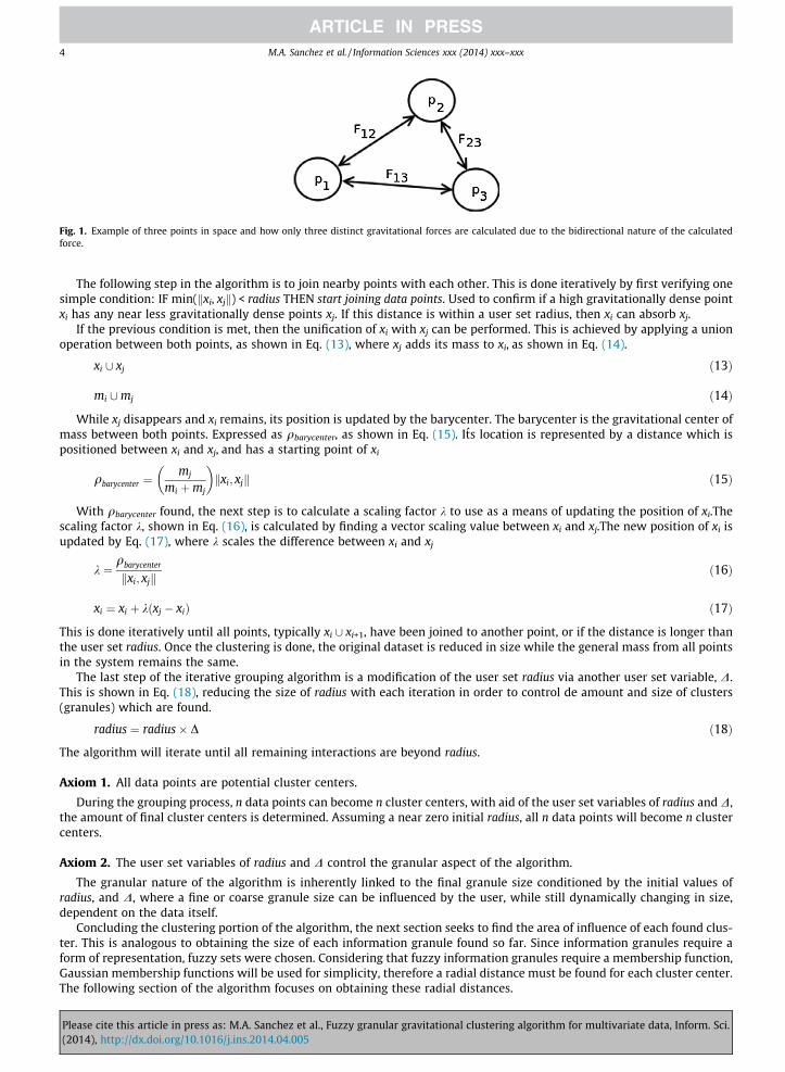
Fig. 1. Example of three points in space and how only three distinct gravitational forces are calculated due to the bidirectional nature of the calculatedforce.


The following step in the algorithm is to join nearby points with each other. This is done iteratively by first verifying onesimple condition: IF min(kxi, xjk) < radius THEN start joining data points. Used to confirm if a high gravitationally dense pointxi has any near less gravitationally dense points xj. If this distance is within a user set radius, then xi can absorb xj.

If the previous condition is met, then the unification of xi with xj can be performed. This is achieved by applying a unionoperation between both points, as shown in Eq. (13), where xj adds its mass to xi, as shown in Eq. (14).

Please(2014

xi [ xj ð13Þ

mi [mj ð14Þ

While xj disappears and xi remains, its position is updated by the barycenter. The barycenter is the gravitational center ofmass between both points. Expressed as qbarycenter, as shown in Eq. (15). Its location is represented by a distance which ispositioned between xi and xj, and has a starting point of xi

qbarycenter ¼mj

mi þmj

� �kxi; xjk ð15Þ

With qbarycenter found, the next step is to calculate a scaling factor k to use as a means of updating the position of xi.Thescaling factor k, shown in Eq. (16), is calculated by finding a vector scaling value between xi and xj.The new position of xi isupdated by Eq. (17), where k scales the difference between xi and xj

k ¼qbarycenter

kxi; xjkð16Þ

xi ¼ xi þ kðxj � xiÞ ð17Þ

This is done iteratively until all points, typically xi [ xi+1, have been joined to another point, or if the distance is longer thanthe user set radius. Once the clustering is done, the original dataset is reduced in size while the general mass from all pointsin the system remains the same.

The last step of the iterative grouping algorithm is a modification of the user set radius via another user set variable, D.This is shown in Eq. (18), reducing the size of radius with each iteration in order to control de amount and size of clusters(granules) which are found.

radius ¼ radius� D ð18Þ

The algorithm will iterate until all remaining interactions are beyond radius.

Axiom 1. All data points are potential cluster centers.

During the grouping process, n data points can become n cluster centers, with aid of the user set variables of radius and D,the amount of final cluster centers is determined. Assuming a near zero initial radius, all n data points will become n clustercenters.

Axiom 2. The user set variables of radius and D control the granular aspect of the algorithm.

The granular nature of the algorithm is inherently linked to the final granule size conditioned by the initial values ofradius, and D, where a fine or coarse granule size can be influenced by the user, while still dynamically changing in size,dependent on the data itself.

Concluding the clustering portion of the algorithm, the next section seeks to find the area of influence of each found clus-ter. This is analogous to obtaining the size of each information granule found so far. Since information granules require aform of representation, fuzzy sets were chosen. Considering that fuzzy information granules require a membership function,Gaussian membership functions will be used for simplicity, therefore a radial distance must be found for each cluster center.The following section of the algorithm focuses on obtaining these radial distances.




Finding the radial distances r for all clusters is performed similarly to how the initial cluster centers were found. Insteadof calculating the gravitational forces between all points, the calculations are done using the found clusters xc against all datapoints x, sans found clusters as defined in Eq. (19). This is done to avoid a division by zero in Eq. (20) when kxc

j ; xik ¼ 0.

Please(2014

xc–xi ð19Þ

Gravitational forces are calculated for each xi against all xcj , as shown in Eq. (20). The xc

j which exerts a higher gravitationalforce unto xi will gain influence upon it, and add xi into a set xsetOfClusterj

.

Fj ¼ Gmc

j mi

kxcj ; xik2 ð20Þ

Having defined where each xi is assigned to a set of xsetOfClusterj, a standard deviation is calculated for each xsetOfClusterj

, shownin Eq. (21). A radial influence rc

k per each k-ith input variable, for all clusters, is obtained. This defines the size of each infor-mation granule.

rck ¼ stdðxsetOfClusterj

Þ ð21Þ

Axiom 3. In some cases any number of xcj will not have influence on any xi in the system.

There will be cases where the mass of some cluster centers will be so small with respect to all other cluster centers that itsr will be zero due to having no gravitational influence on any data point in the system. When this is the case, the clustercenter will disappear since it has no impact on the system.

With the centers and granule sizes found, the next and final step is to calculate the Takagi–Sugeno–Kang (TSK) conse-quent parameters which construct a Fuzzy Inference System (FIS), which in this case is a 1st Order TSK FIS. This is doneby applying a known method which relies on the Least Square Estimation method (LSE) [11] to adjust the parameters ofthe consequents based on the known antecedents.

The adjustment considers c cluster centers fx�1; x�2; . . . ; x�cg with n-space dimensions. The input variables (input space) arerepresented by y�i , and the output variables (output space) are represented by z�i . Where z�i is in the form of a 1st Order linearfunction, as shown in Eq. (22), where Gi are the input constant parameters, and hi the constants for each z�i .

z�i ¼ Giyþ hi ð22Þ

Considering each x�i describes a fuzzy rule, and having a copy of the training data x, the firing strengths xi per each ruleare calculated by Eq. (23), considering all membership functions are Gaussians. Where each xi is used alongside the obtainedrc and xc.

xi ¼ e�12

xi�xc

rc

�� 2

ð23Þ

A parameter si must be defined in order to use LSE, shown in Eq. (24). This can be rewritten as Eq. (25). Now, z�i can bedefined to the form shown in Eq. (26), which describes a matrix of parameters to be optimized by the LSE method, taking theform of AX = B.

si ¼xiPcj¼1xi

ð24Þ

z ¼Xc

i�1

siz�i ¼Xc

i¼1

siðGixþ hiÞ ð25Þ

zT1

..

.

zTn

2664

3775 ¼

s1;1xT1 s1;1 � � � sc;1xT

1 sc;1

..

.

s1;nxTn s1;n � � � sc;nxT

n sc;n

2664

3775

GT1

hT1

..

.

GTc

hTc

2666666664

3777777775

ð26Þ

where

B ¼

zT1

..

.

zTn

2664

3775 ð27Þ




Please(2014

A ¼

s1;1xT1 s1;1 � � � sc;1xT

1 sc;1

..

.

s1;nxTn s1;n � � � sc;nxT

n sc;n

2664

3775 ð28Þ

X ¼

GT1

hT1

..

.

GTc

hTc

2666666664

3777777775

ð29Þ

Knowing that LSE has the form AX = B, where B is a matrix of the output values, A is a matrix of constants, and X is a matrixof estimated parameters. The final solution is given by Eq. (30).

X ¼ ðAT AÞ�1

AT B ð30Þ

3.1. Algorithms

The main algorithm of FGGCA is separated into two sub-procedures: the clustering section, and the granule size section.Both are shown in the following pseudo-code, as well as the main algorithm.

3.1.1. Find the granular centersThe first sub-procedure of the FGGCA: findClusters, searches for the cluster centers which better represents the data x. It

receives a copy of the dataset x, and the user set values of radius and D. When the procedure ends, it returns a copy of theclusters centers.

procedure findClusters(x,radius, D)1. LOOP while INTERACTIONS_EXIST==TRUE2. INTERACTIONS_EXIST=FALSE; initialize exit condition for clustering3. Fij ¼ G mimj

kxi ;xjk2 ; calculate all interacting gravitational forces in the system, where i – j

4. Fdensityi ¼

Pnj¼1Fij; calculate the gravitational density of Fi

5. x ¼ sortðx; Fdensityi Þ; sort x in reference to Fdensity

i : Where the xi with the highest gravitational density is set as thefirst value in x, and each xi is subsequently set as the gravitational density is reduced

6. LOOP foreach i in xi

7. IF min(kxi, xjk) < radius THEN; verify if there are points which can interact and join together, where i – j8. INTERACTIONS_EXIST=TRUE; indicate that another iteration can be done9. mi [mj; join the mass of xj unto xi

10. qbarycenter ¼mj

miþmj

� �kxi; xjk; calculate the barycenter distance between xi and xj

11. k ¼ qbarycenter

kxi ;xjk ; calculate a scaling factor k

12. xi ¼ xi þ kðxj � xiÞ; update de position of xi to its new location, based on k

13. radius = radius � D; update the value of radius in relation to D14. RETURN x

3.1.2. Find the size of the granulesThis sub-procedure, named findSizeOfGranules, has the task of finding a sub-optimal granule size. It receives a copy of the

dataset x, and the set of clusters xc previously found by the procedure findClusters. When the procedure ends, it returns a setof rc which store the individual granule size for each cluster center.

procedure findSizeOfGranules(x, xc)

1. Fj ¼ Gmc

j mi

kxcj ;xik2 ; calculate all interacting gravitational forces in the system, where xc

j –xi

2. Findexj ¼maxðFjÞ; find the index of Fj which exerts a higher gravitational force.

3. xsetOfClusterj¼ xFindex

j; assign to a set of xsetOfClusterj

the value of xi which index is Findexj

4. LOOP foreach k in NumberOfInputs(x)5. rc

k ¼ stdðxsetOfClusterjÞ; calculate the standard deviation for each input variable of each cluster

6. RETURN rc




3.1.3. Main FGGCA algorithm
The main procedure of the FGGCA algorithm is defined by two sub-procedures which contribute to finding the location of
each cluster center xc and the granule size rc for each one, followed by a section where TSK consequent parameters areobtained through LSE method. It receives a copy of the dataset x, and the user set values of radius and D.

When the procedure ends, it returns three sets of parameters, the first two, used for forming antecedents in a FIS: clustercenters xc, and granule sizes rc. The third, used for forming 1st Order linear functions: estimated parameters X. With bothantecedent and consequent parameters a TSK FIS can be formed.

procedure FGGCA(x,radius, D)xc = findClusters(x, radius, D)2. rc = findSizeOfGranules(x, xc)

3. xi ¼ e�12

xi�xc

rc

�� 2

; obtain all firing strengths per each xi

4. X = (ATA)�1ATB; where A, B, and X are represented by Eqs. (27)–(29), evaluate with xi and xi

5. RETURN (xc, rc, X)

3.2. Algorithm order

This type of gravitational simulation is usually O(n3), because with each calculation of gravitational forces, all the pointsmove based on Newtons second law of motion, thus having to update the position of all points each iteration. Since the aimof this algorithm is to find the most influential gravitational centers in the data, no constant motion is needed. Consideringthat the amount of data points is greatly reduced with each iteration, up to half the set each time, it can be perceived that thisalgorithm in general is O(n2).

4. Experimental results

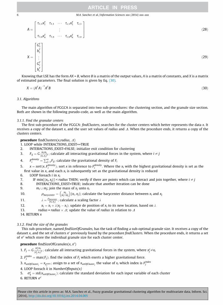
Various experiments were performed with FGGCA. The first example is with a synthetic dataset which was designed withthe purpose of highlighting the main properties of the FGGCA. As shown in Fig. 2, this dataset was created to have a biastoward the left side of the cluster by having a higher concentration of data points on that side. This shows how the algorithm,through the theory of gravitational density, finds the location which best represents the data, and not just the geometricalcenter of the data. The second aim of this example is to show the coverage of r on both axes. Because Gaussian membershipfunctions are used to represent the coverage, the length of r should not cover all data, as the Gaussian functions would over-extend and become too generalized. In this example, the mentioned behavior does not occur, and the length of r has a betterrepresentation of how data is dispersed.

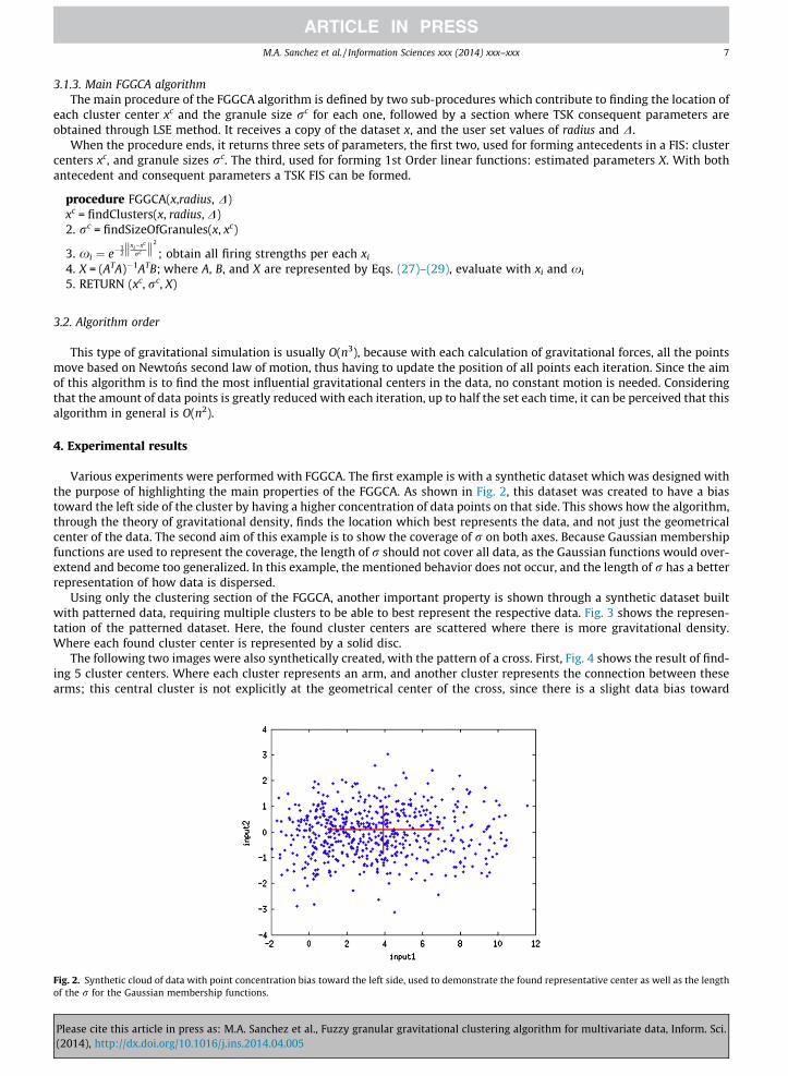
Using only the clustering section of the FGGCA, another important property is shown through a synthetic dataset builtwith patterned data, requiring multiple clusters to be able to best represent the respective data. Fig. 3 shows the represen-tation of the patterned dataset. Here, the found cluster centers are scattered where there is more gravitational density.Where each found cluster center is represented by a solid disc.

The following two images were also synthetically created, with the pattern of a cross. First, Fig. 4 shows the result of find-ing 5 cluster centers. Where each cluster represents an arm, and another cluster represents the connection between thesearms; this central cluster is not explicitly at the geometrical center of the cross, since there is a slight data bias toward

Fig. 2. Synthetic cloud of data with point concentration bias toward the left side, used to demonstrate the found representative center as well as the lengthof the r for the Gaussian membership functions.

Please cite this article in press as: M.A. Sanchez et al., Fuzzy granular gravitational clustering algorithm for multivariate data, Inform. Sci.(2014), http://dx.doi.org/10.1016/j.ins.2014.04.005


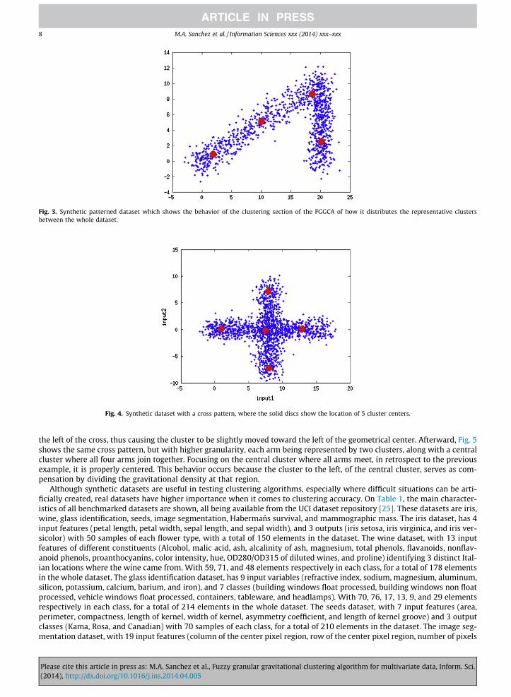
Fig. 3. Synthetic patterned dataset which shows the behavior of the clustering section of the FGGCA of how it distributes the representative clustersbetween the whole dataset.

Fig. 4. Synthetic dataset with a cross pattern, where the solid discs show the location of 5 cluster centers.


the left of the cross, thus causing the cluster to be slightly moved toward the left of the geometrical center. Afterward, Fig. 5shows the same cross pattern, but with higher granularity, each arm being represented by two clusters, along with a centralcluster where all four arms join together. Focusing on the central cluster where all arms meet, in retrospect to the previousexample, it is properly centered. This behavior occurs because the cluster to the left, of the central cluster, serves as com-pensation by dividing the gravitational density at that region.

Although synthetic datasets are useful in testing clustering algorithms, especially where difficult situations can be arti-ficially created, real datasets have higher importance when it comes to clustering accuracy. On Table 1, the main character-istics of all benchmarked datasets are shown, all being available from the UCI dataset repository [25]. These datasets are iris,wine, glass identification, seeds, image segmentation, Habermans survival, and mammographic mass. The iris dataset, has 4input features (petal length, petal width, sepal length, and sepal width), and 3 outputs (iris setosa, iris virginica, and iris ver-sicolor) with 50 samples of each flower type, with a total of 150 elements in the dataset. The wine dataset, with 13 inputfeatures of different constituents (Alcohol, malic acid, ash, alcalinity of ash, magnesium, total phenols, flavanoids, nonflav-anoid phenols, proanthocyanins, color intensity, hue, OD280/OD315 of diluted wines, and proline) identifying 3 distinct Ital-ian locations where the wine came from. With 59, 71, and 48 elements respectively in each class, for a total of 178 elementsin the whole dataset. The glass identification dataset, has 9 input variables (refractive index, sodium, magnesium, aluminum,silicon, potassium, calcium, barium, and iron), and 7 classes (building windows float processed, building windows non floatprocessed, vehicle windows float processed, containers, tableware, and headlamps). With 70, 76, 17, 13, 9, and 29 elementsrespectively in each class, for a total of 214 elements in the whole dataset. The seeds dataset, with 7 input features (area,perimeter, compactness, length of kernel, width of kernel, asymmetry coefficient, and length of kernel groove) and 3 outputclasses (Kama, Rosa, and Canadian) with 70 samples of each class, for a total of 210 elements in the dataset. The image seg-mentation dataset, with 19 input features (column of the center pixel region, row of the center pixel region, number of pixels



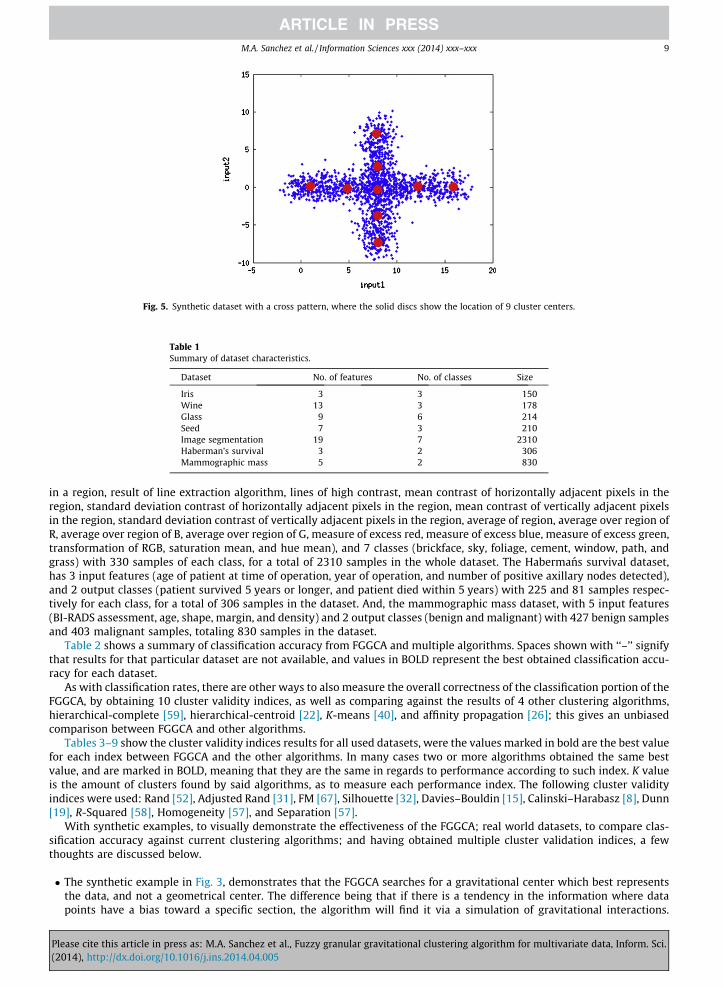
Fig. 5. Synthetic dataset with a cross pattern, where the solid discs show the location of 9 cluster centers.

Table 1Summary of dataset characteristics.

Dataset No. of features No. of classes Size

Iris 3 3 150Wine 13 3 178Glass 9 6 214Seed 7 3 210Image segmentation 19 7 2310Haberman’s survival 3 2 306Mammographic mass 5 2 830


in a region, result of line extraction algorithm, lines of high contrast, mean contrast of horizontally adjacent pixels in theregion, standard deviation contrast of horizontally adjacent pixels in the region, mean contrast of vertically adjacent pixelsin the region, standard deviation contrast of vertically adjacent pixels in the region, average of region, average over region ofR, average over region of B, average over region of G, measure of excess red, measure of excess blue, measure of excess green,transformation of RGB, saturation mean, and hue mean), and 7 classes (brickface, sky, foliage, cement, window, path, andgrass) with 330 samples of each class, for a total of 2310 samples in the whole dataset. The Habermans survival dataset,has 3 input features (age of patient at time of operation, year of operation, and number of positive axillary nodes detected),and 2 output classes (patient survived 5 years or longer, and patient died within 5 years) with 225 and 81 samples respec-tively for each class, for a total of 306 samples in the dataset. And, the mammographic mass dataset, with 5 input features(BI-RADS assessment, age, shape, margin, and density) and 2 output classes (benign and malignant) with 427 benign samplesand 403 malignant samples, totaling 830 samples in the dataset.

Table 2 shows a summary of classification accuracy from FGGCA and multiple algorithms. Spaces shown with ‘‘–’’ signifythat results for that particular dataset are not available, and values in BOLD represent the best obtained classification accu-racy for each dataset.

As with classification rates, there are other ways to also measure the overall correctness of the classification portion of theFGGCA, by obtaining 10 cluster validity indices, as well as comparing against the results of 4 other clustering algorithms,hierarchical-complete [59], hierarchical-centroid [22], K-means [40], and affinity propagation [26]; this gives an unbiasedcomparison between FGGCA and other algorithms.

Tables 3–9 show the cluster validity indices results for all used datasets, were the values marked in bold are the best valuefor each index between FGGCA and the other algorithms. In many cases two or more algorithms obtained the same bestvalue, and are marked in BOLD, meaning that they are the same in regards to performance according to such index. K valueis the amount of clusters found by said algorithms, as to measure each performance index. The following cluster validityindices were used: Rand [52], Adjusted Rand [31], FM [67], Silhouette [32], Davies–Bouldin [15], Calinski–Harabasz [8], Dunn[19], R-Squared [58], Homogeneity [57], and Separation [57].

With synthetic examples, to visually demonstrate the effectiveness of the FGGCA; real world datasets, to compare clas-sification accuracy against current clustering algorithms; and having obtained multiple cluster validation indices, a fewthoughts are discussed below.

� The synthetic example in Fig. 3, demonstrates that the FGGCA searches for a gravitational center which best representsthe data, and not a geometrical center. The difference being that if there is a tendency in the information where datapoints have a bias toward a specific section, the algorithm will find it via a simulation of gravitational interactions.



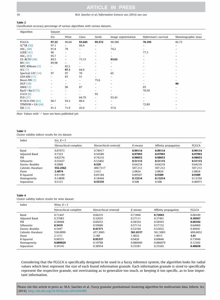
Table 2Classification accuracy percentage of various algorithms with various datasets.

Algorithm Dataset

Iris Wine Glass Seeds Image segmentation Haberman’s survival Mammographic mass

FGGCA 97.22 96.66 93.645 95.572 90.586 76.195 82.72SC3SR [50] 97.1 – 66.4 – – – –ASC1 [60] 91.8 70 – – 74.2 – –LODE [41] 96 – – – – 77.3 –ASC2 [63] 95.7 – – – – – –CE–RCTO [68] 89.5 – 73.15 – 93.63 – –BH [30] 89.98 – – – – – –MPC-KMeans [5] – 82.2 – – – – –SCC [7] – 97.1 64.9 – – – –Spectral CAT [14] 97 97 70 – 65 – –LDA-KM [17] – 83 51 – – – –Boost-NN [1] – – – 75.6 – – –DGP [39] – – – – – – 86AMA[13] – 96 87 – – 65 –Bac0 + Bac1[73] – – – – – 70.59 –CGCA [9] – – – 92 – – –FLD [27] – – 64.79 – 93.43 – –IP-DCA-VNS [61] 96.7 93.2 80.4 – – – –TPMSVM + GA [64] – – – – – 72.89 –DJS [12] 91.3 71.9 43.9 – 57.6 – –

Note: Values with ‘–’ have not been published yet.

Table 3Cluster validity indices results for iris dataset.

Index Iris, K = 3

Hierarchical-complete Hierarchical-centroid K-means Affinity propagation FGGCA

Rand 0.87973 0.78917 0.99114 0.99114 0.99114Adjusted Rand 0.7323 0.56589 0.97993 0.97993 0.97993FM 0.82376 0.74216 0.98653 0.98653 0.98653Silhouette 0.55437 0.53402 0.51115 0.51115 0.51115Davies–Bouldin 0.5808 0.529 0.64218 0.64218 0.64218Calinski–Harabasz 552.2562 400.7317 507.212 507.212 507.212Dunn 2.4074 2.412 2.0824 2.0824 2.0824R-Squared 0.91189 0.85184 0.89567 0.9309 0.9309Homogeneity 0.14898 0.18444 0.13214 0.13214 0.13356Separation 0.5121 0.55335 0.508 0.508 0.46973

Table 4Cluster validity indices results for wine dataset.

Index Wine, K = 3




Considering that the FGGCA is specifically designed to be used in a fuzzy inference system, the algorithm looks for radialvalues which best represent the size of each found information granule. Each information granule is sized to specificallyrepresent the respective granule, not overtraining as to generalize too much, or keeping it too specific, as to lose impor-tant information.



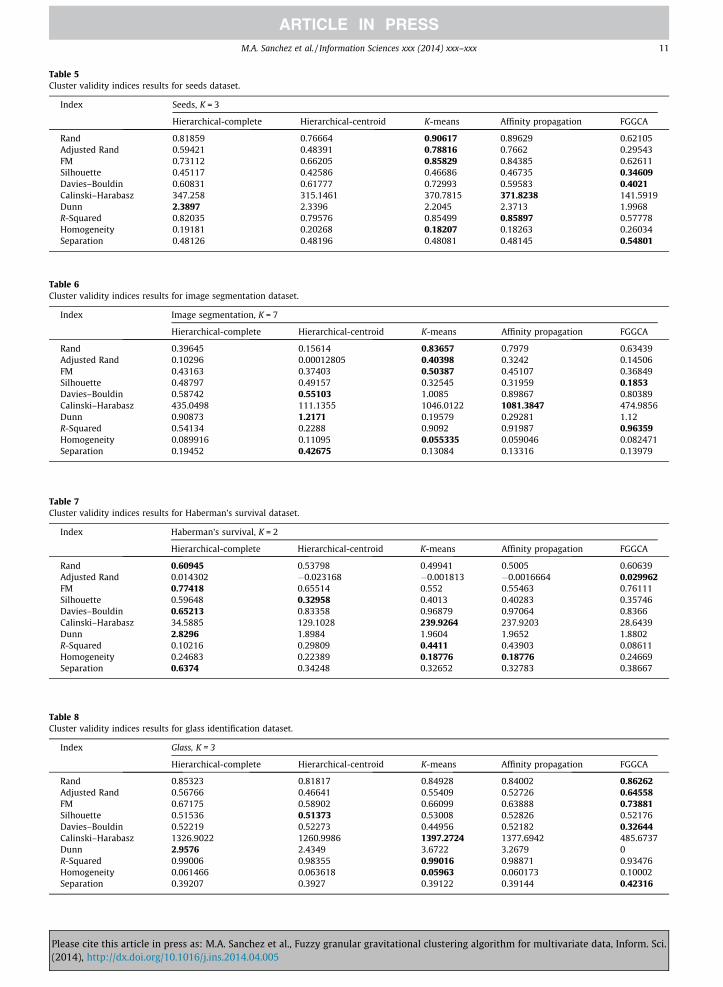
Table 5Cluster validity indices results for seeds dataset.

Index Seeds, K = 3



Table 6Cluster validity indices results for image segmentation dataset.

Index Image segmentation, K = 7



Table 7Cluster validity indices results for Haberman’s survival dataset.

Index Haberman’s survival, K = 2


Rand 0.60945 0.53798 0.49941 0.5005 0.60639Adjusted Rand 0.014302 �0.023168 �0.001813 �0.0016664 0.029962FM 0.77418 0.65514 0.552 0.55463 0.76111Silhouette 0.59648 0.32958 0.4013 0.40283 0.35746Davies–Bouldin 0.65213 0.83358 0.96879 0.97064 0.8366Calinski–Harabasz 34.5885 129.1028 239.9264 237.9203 28.6439Dunn 2.8296 1.8984 1.9604 1.9652 1.8802R-Squared 0.10216 0.29809 0.4411 0.43903 0.08611Homogeneity 0.24683 0.22389 0.18776 0.18776 0.24669Separation 0.6374 0.34248 0.32652 0.32783 0.38667

Table 8Cluster validity indices results for glass identification dataset.

Index Glass, K = 3


Rand 0.85323 0.81817 0.84928 0.84002 0.86262Adjusted Rand 0.56766 0.46641 0.55409 0.52726 0.64558FM 0.67175 0.58902 0.66099 0.63888 0.73881Silhouette 0.51536 0.51373 0.53008 0.52826 0.52176Davies–Bouldin 0.52219 0.52273 0.44956 0.52182 0.32644Calinski–Harabasz 1326.9022 1260.9986 1397.2724 1377.6942 485.6737Dunn 2.9576 2.4349 3.6722 3.2679 0R-Squared 0.99006 0.98355 0.99016 0.98871 0.93476Homogeneity 0.061466 0.063618 0.05963 0.060173 0.10002Separation 0.39207 0.3927 0.39122 0.39144 0.42316




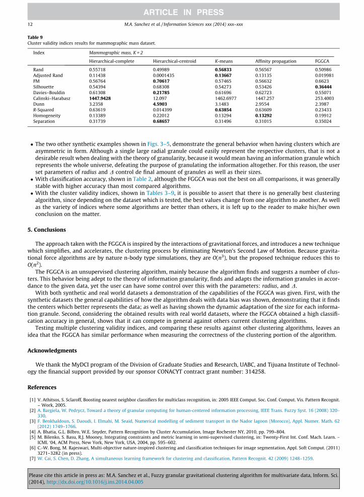
Table 9Cluster validity indices results for mammographic mass dataset.

Index Mammographic mass, K = 2




� The two other synthetic examples shown in Figs. 3–5, demonstrate the general behavior when having clusters which areasymmetric in form. Although a single large radial granule could easily represent the respective clusters, that is not adesirable result when dealing with the theory of granularity, because it would mean having an information granule whichrepresents the whole universe, defeating the purpose of granulating the information altogether. For this reason, the userset parameters of radius and D control de final amount of granules as well as their sizes.� With classification accuracy, shown in Table 2, although the FGGCA was not the best on all comparisons, it was generally

stable with higher accuracy than most compared algorithms.� With the cluster validity indices, shown in Tables 3–9, it is possible to assert that there is no generally best clustering

algorithm, since depending on the dataset which is tested, the best values change from one algorithm to another. As wellas the variety of indices where some algorithms are better than others, it is left up to the reader to make his/her ownconclusion on the matter.

5. Conclusions

The approach taken with the FGGCA is inspired by the interactions of gravitational forces, and introduces a new techniquewhich simplifies, and accelerates, the clustering process by eliminating Newton’s Second Law of Motion. Because gravita-tional force algorithms are by nature n-body type simulations, they are O(n3), but the proposed technique reduces this toO(n2).

The FGGCA is an unsupervised clustering algorithm, mainly because the algorithm finds and suggests a number of clus-ters. This behavior being adept to the theory of information granularity, finds and adapts the information granules in accor-dance to the given data, yet the user can have some control over this with the parameters: radius, and D.

With both synthetic and real world datasets a demonstration of the capabilities of the FGGCA was given. First, with thesynthetic datasets the general capabilities of how the algorithm deals with data bias was shown, demonstrating that it findsthe centers which better represents the data; as well as having shown the dynamic adaptation of the size for each informa-tion granule. Second, considering the obtained results with real world datasets, where the FGGCA obtained a high classifi-cation accuracy in general, shows that it can compete in general against others current clustering algorithms.

Testing multiple clustering validity indices, and comparing these results against other clustering algorithms, leaves anidea that the FGGCA has similar performance when measuring the correctness of the clustering portion of the algorithm.

Acknowledgments

We thank the MyDCI program of the Division of Graduate Studies and Research, UABC, and Tijuana Institute of Technol-ogy the financial support provided by our sponsor CONACYT contract grant number: 314258.

References

[1] V. Athitsos, S. Sclaroff, Boosting nearest neighbor classifiers for multiclass recognition, in: 2005 IEEE Comput. Soc. Conf. Comput. Vis. Pattern Recognit.– Work, 2005.

[2] A. Bargiela, W. Pedrycz, Toward a theory of granular computing for human-centered information processing, IEEE Trans. Fuzzy Syst. 16 (2008) 320–330.

[3] F. Benkhaldoun, S. Daoudi, I. Elmahi, M. Seaid, Numerical modelling of sediment transport in the Nador lagoon (Morocco), Appl. Numer. Math. 62(2012) 1749–1766.

[4] A. Bhatia, G.L. Bilbro, W.E. Snyder, Pattern Recognition by Cluster Accumulation, Image Rochester NY, 2010, pp. 799–804.[5] M. Bilenko, S. Basu, R.J. Mooney, Integrating constraints and metric learning in semi-supervised clustering, in: Twenty-First Int. Conf. Mach. Learn. –

ICML ‘04, ACM Press, New York, New York, USA, 2004, pp. 595–602.[6] C.-W. Bong, M. Rajeswari, Multi-objective nature-inspired clustering and classification techniques for image segmentation, Appl. Soft Comput. (2011)

3271–3282 (in press).[7] W. Cai, S. Chen, D. Zhang, A simultaneous learning framework for clustering and classification, Pattern Recognit. 42 (2009) 1248–1259.


http://refhub.elsevier.com/S0020-0255(14)00452-6/h0010







[8] T. Calinski, J. Harabasz, A dendrite method for cluster analysis, Commun. Stat. – Theory Methods 3 (1974) 1–27.[9] M. Charytanowicz, J. Niewczas, Complete gradient clustering algorithm for features analysis of X-ray images, Adv. Intell. Soft Comp. 69 (2010) 15–24.

[10] M.-Y. Chen, A hybrid ANFIS model for business failure prediction utilizing particle swarm optimization and subtractive clustering, Inf. Sci. (Ny) 220(2013) 180–195.

[11] S.L. Chiu, Fuzzy model identification based on cluster estimation, J. Intell. Fuzzy Syst. 2 (1994) 267–278.[12] A. Daneshgar, R. Javadi, B.S. Razavi, Clustering using isoperimetric number of trees, Pattern Recognit. 46 (2012) 3371–3382.[13] D. Dash, G.F. Cooper, Model averaging for prediction with discrete bayesian networks, J. Mach. Learn. Res. 5 (2004) 1177–1203.[14] G. David, A. Averbuch, SpectralCAT: categorical spectral clustering of numerical and nominal data, Pattern Recognit. 45 (2012) 416–433.[15] D.L. Davies, D.W. Bouldin, A cluster separation measure, IEEE Trans. Pattern Anal. Mach. Intell. PAMI-1 (1979) 224–227.[16] M. Dillon, The use of clustering techniques in the analysis of judicial prose, Inf. Sci. (Ny) 8 (1975) 95–107.[17] C. Ding, T. Li, Adaptive dimension reduction using discriminant analysis and k-means clustering, in: Int. Conf. Mach. Learn, ACM Press, New York, New

York, USA, 2007. pp. 521–528.[18] B. Dogan, M. Korürek, A new ECG beat clustering method based on kernelized fuzzy c-means and hybrid ant colony optimization for continuous

domains, Appl. Soft Comput. 12 (2012) 3442–3451.[19] J.C. Dunn, Well-separated clusters and optimal fuzzy partitions, J. Cybern. 4 (1974) 95–104.[20] R.M. Duwairi, Clustering semantically related classes in a heterogeneous multidatabase system, Inf. Sci. (Ny) 162 (2004) 193–210.[21] M. Ester, H. Kriegel, J. Sander, X. Xu, A density-based algorithm for discovering clusters in large spatial databases with noise, Computer(Long. Beach.

Calif) 1996 (1996) 226–231.[22] B.S. Everitt, A finite mixture model for the clustering of mixed-mode data, Stat. Probab. Lett. 6 (1988) 305–309.[23] M.H. Fazel Zarandi, R. Gamasaee, I.B. Turksen, A type-2 fuzzy c-regression clustering algorithm for Takagi–Sugeno system identification and its

application in the steel industry, Inf. Sci. (Ny) 187 (2012) 179–203.[24] A. Foroush Bastani, Z. Ahmadi, D. Damircheli, A Radial basis collocation method for pricing American options under regime-switching jump-diffusion

models, Appl. Numer. Math. 65 (2013) 79–90.[25] A. Frank, A. Asuncion, UCI machine learning repository, Univ. Calif. Irvine Sch. Inf. 2008 (2010).[26] B.J. Frey, D. Dueck, Clustering by passing messages between data points, Science 315 (2007) 972–976.[27] D. Gao, D. Jun, Z. Changming, Integrated Fisher linear discriminants: an empirical study, Pattern Recognit. 47 (2013) 789–805.[28] J. Gomez, D. Dasgupta, O. Nasraoui, A new gravitational clustering algorithm, in: Proc. SIAM Int. Conf. Data Min., 2003.[29] J. Gomez, O. Nasraoui, E. Leon, RAIN: data clustering using randomized interactions between data points, in: Int. Conf. Mach. Learn. Appl. 2004.

Proceedings., IEEE, 2004, pp. 250–255.[30] A. Hatamlou, Black hole: a new heuristic optimization approach for data clustering, Inf. Sci. (Ny) 222 (2013) 175–184.[31] L. Hubert, P. Arabie, Comparing partitions, J. Classif. 2 (1985) 193–218.[32] L. Kaufman, P.J. Rousseeuw, Finding groups in data: an introduction to cluster analysis, John Wiley and Sons, New York, 1990.[33] A. Kulkarni, V. Muniganti, Fuzzy neural network models for clustering, in: Proc. 1996 ACM Symp. Appl. Comput., ACM, 1996, pp. 523–528.[34] S. Kundu, Gravitational clustering: a new approach based on the spatial distribution of the points, Pattern Recognit. 32 (1999) 1149–1160.[35] O. Linda, M. Manic, General type-2 fuzzy C-means algorithm for uncertain fuzzy clustering, IEEE Trans. Fuzzy Syst. 20 (5) (2012) 883–897.[36] H. Liu, F. Zhao, L. Jiao, Fuzzy spectral clustering with robust spatial information for image segmentation, Appl. Soft Comput. 12 (2012) 3636–3647.[37] X. Liu, H. Fu, An effective clustering algorithm with ant colony, J. Comput. 5 (2010) 598–605.[38] T. Long, L.-W. Jin, A new simplified gravitational clustering method for multi-prototype learning based on minimum classification error training, in: N.

Zheng, X. Jiang, X. Lan (Eds.), Adv. Mach. Vision, Image Process. Pattern Anal. Int. Work. Intell. Comput. Pattern Anal., Springer Berlin Heidelberg, Berlin,Heidelberg, 2006, pp. 168–175.

[39] S.A. Ludwig, Prediction of breast cancer biopsy outcomes using a distributed genetic programming approach, in: T.C. Veinot, Ü.V. Çatalyürek, G. Luo, H.Andrade, N.R. Smalheiser (Eds.), Proc. 1st ACM Int. Heal. Informatics Symp., ACM, 2010, pp. 694–699.

[40] J. Macqueen, Some Methods for classification and analysis of multivariate observations, in: Proc. of the fifth Berkeley Symp. Math. Stat. Probab. vol. 1,University of California Press, 1967, pp. 281–297.

[41] R. Meo, D. Bachar, D. Ienco, LODE: a distance-based classifier built on ensembles of positive and negative observations, Pattern Recognit. 45 (2012)1409–1425.

[42] M. Muhieddine, É. Canot, R. March, Heat transfer modeling in saturated porous media and identification of the thermophysical properties of the soil byinverse problem, Appl. Numer. Math. 62 (2012) 1026–1040.

[43] F. Naghdy, Fuzzy clustering of human motor motion, Appl. Soft Comput. 11 (2011) 927–935.[44] I. Newton, Philosophiæ naturalis principia mathematica, Cambridge Digital Library, 1687, Retrieved 3 July 2013.[45] R. Nock, F. Nielsen, On weighting clustering, IEEE Trans. Pattern Anal. Mach. Intell. 28 (2006) 1223–1235.[46] W. Pedrycz, Conditional fuzzy C-means, Pattern Recognit. Lett. 17 (1996) 625–631.[47] W. Pedrycz, Granular computing – the emerging paradigm, J. Uncertain Syst. 1 (2007) 38–61.[48] W. Pedrycz, G. Vukovich, Granular computing with shadowed sets, Int. J. Intell. Syst. 17 (2002) 173–197.[49] X. Peng, D. Xu, Twin Mahalanobis distance-based support vector machines for pattern recognition, Inf. Sci. (Ny) 200 (2012) 22–37.[50] Q. Qian, S. Chen, W. Cai, Simultaneous clustering and classification over cluster structure representation, Pattern Recognit. 45 (2012) 2227–2236.[51] G.N. Ramos, Y. Hatakeyama, F. Dong, K. Hirota, Hyperbox clustering with Ant Colony Optimization (HACO) method and its application to medical risk

profile recognition, Appl. Soft Comput. 9 (2009) 632–640.[52] W.M. Rand, Objective criteria for the evaluation of clustering methods, J. Am. Stat. Assoc. 66 (1971) 846–850.[53] E. Rashedi, H. Nezamabadi-pour, A stochastic gravitational approach to feature based color image segmentation, Eng. Appl. Artif. Intell. 26 (2013)

1322–1332.[54] E. Rashedi, H. Nezamabadi-pour, S. Saryazdi, GSA: a gravitational search algorithm, Inf. Sci. (Ny) 179 (2009) 2232–2248.[55] Y.S.Y. Sai, P.N.P. Nie, D.C.D. Chu, A model of granular computing based on rough set theory, Stud. Fuzziness Soft Comput. 294 (2013) 239–263.[56] M.A. Sanchez, O. Castillo, J.R. Castro, A. Rodríguez-Díaz, Fuzzy granular gravitational clustering algorithm, in: North Am. Fuzzy Inf. Process. Soc. 2012,

2012.[57] R. Shamir, R. Sharan, Algorithmic approaches to clustering gene expression data, Curr. Top. Comput. Biol. (2001) 269–300.[58] S. Sharma, Applied Multivariate Techniques, John Wiley & Sons, Inc.,, 1995.[59] T. Sørensen, A method of establishing groups of equal amplitude in plant sociology based on similarity of species and its application to analyses of the

vegetation on Danish commons, Biol. Skr. 5 (1948) 1–34.[60] K. Tas�demir, Vector quantization based approximate spectral clustering of large datasets, Pattern Recognit. 45 (2012) 3034–3044.[61] L. Thi, H. An, L. Hoai, P. Dinh, New and efficient DCA based algorithms for minimum sum-of-squares clustering, Pattern Recognit. 47 (2014) 388–401.[62] S. Thomassey, M. Happiette, A neural clustering and classification system for sales forecasting of new apparel items, Appl. Soft Comput. 7 (2007) 1177–

1187.[63] V.-V. Vu, N. Labroche, B. Bouchon-Meunier, Improving constrained clustering with active query selection, Pattern Recognit. 45 (2012) 1749–1758.[64] Z. Wang, Y.-H. Shao, T.-R. Wu, A GA-based model selection for smooth twin parametric-margin support vector machine, Pattern Recognit. 46 (2013)

2267–2277.[65] A.K.C. Wong, D.K.Y. Chiu, W. Huang, A discrete-valued clustering algorithm with applications to biomolecular data, Inf. Sci. (Ny) 139 (2001) 97–112.[66] W.E. Wright, Gravitational clustering, Pattern Recognit. 9 (1977) 151–166.[67] K.Y. Yeung, D.R. Haynor, W.L. Ruzzo, Validating clustering for gene expression data, Bioinformatics. 17 (2001) 309–318.


























































































[68] Z. Yu, H.-S. Wong, J. You, G. Yu, G. Han, Hybrid cluster ensemble framework based on the random combination of data transformation operators,Pattern Recognit. 45 (2012) 1826–1837.

[69] H.C. Yung, Segmentation of color images based on the gravitational clustering concept, Opt. Eng. 37 (1998) 989–1000.[70] L.A. Zadeh, Fuzzy sets, Inf. Control. 8 (1965) 338–353.[71] L.Z.L. Zhang, B.Z.B. Zhang, Quotient space based multi-granular computing, Stud. Comput. Intelligence 547 (2014).[72] T. Zhang, H. Qu, An Improved Clustering Algorithm, in: Proc. Third Int. Symp. Comput. Sci. Comput. Technol., Jiaozuo, China, 2010, pp. 112–115.[73] Y.Z.Y. Zhang, W.N. Street, Bagging with adaptive costs, IEEE Trans. Knowl. Data Eng. 20 (2008).[74] Y.Z.Y. Zhang, X.Z.X. Zhu, Z.H.Z. Huang, Fuzzy sets based granular logics for granular computing, Stud. Comput. Intelligence 547 (2014).










fuzzy granular gravitational clustering algorithm for multivariate data

Documents