Steady Flow and its Instability

of Gravitational Granular Flow

Namiko Mitarai

Department of Chemistry and Physics of Condensed Matter,

Graduate School of Science, Kyushu University, Japan.

A thesis submitted for the degree of Doctor of Science

Kyushu University

January 2003

Abstract

Granular matter consists of a large number of macroscopic particles; the

thermal noise has no effect on the particle motion and the interactions are

dissipative. These features make the granular flow very different from molec-

ular fluids.

One of the simplest situations to see the complex behavior of granular flow

is the gravitational granular flow on a slope. When the inclination angle is

small enough, the material stays at rest. The material begins to flow beyond a

critical angle; the interaction between the particles is dominated by sustained

contacts in the dense and slow flow for the small inclination angle, while the

low-density rapid flow is realized for the large enough inclination, where the

interaction is dominated by inelastic collisions. Understanding these flowing

behaviors is a challenging problem of non-equilibrium statistical physics, not

to mention its technological importance. In this thesis, we investigate the

fundamental properties of gravitational granular flow. We study the steady

flow and its instability by molecular dynamics simulations, and analyze the

steady flow by a hydrodynamic model.

Firstly, we clarify the difference between the low-density collisional flow

and the dense frictional flow. In the molecular dynamics simulation of the

granular material, the soft sphere model with elastic force and dissipation

is often used. We examine how the dynamical behavior of steady granular

flow changes in the inelastic hard sphere limit of the soft sphere model with

keeping the restitution coefficient constant. We find distinctively different

limiting behaviors for the two flow regimes, i.e., the collisional flow and the

frictional flow. In the collisional flow, the hard sphere limit is straightforward;

the number of collisions per particle per unit time converges to a finite value

and the total contact time fraction with other particles goes to zero. For

the frictional flow, however, we demonstrate that the collision rate diverges

as a power of the particle stiffness so that the time fraction of the multiple

contacts remains finite even in the hard sphere limit although the contact

time fraction for binary collisions tends to zero.

The second subject is to test the applicability of a continuum model to the

collisional granular flow in which spinning motion of each grain is considered.

In granular material, the angular momentum of the spinning motion is not

always negligible because of their macroscopic size. It is known that the mean

spin often deviates from the vorticity of the mean velocity near the boundary.

Such a deviation may affect the flow behavior through the coupling of the

particle spin and the velocity field. We apply the micropolar fluid model

to the collisional flow, which is a continuum model in which the angular

velocity field is considered as well as the density and the velocity fields. We

demonstrate that, using a simple estimate for the parameters in the theory,

the model equations quantitatively reproduce the velocity and the angular

velocity profiles obtained from the numerical simulation of the rapid granular

flow on a slope.

Finally, we investigate the steady granular flow on a slope and its instabil-

ity in the low-density regime using the molecular dynamics simulation. We

determine the parameter region where the steady collisional flow is realized

upon changing the inclination angle and the density of particles. Then we

demonstrate that, when the system size is long enough, the collisional gran-

ular flow shows clustering instability. It is shown that the uniform flow is

less stable for longer system size and/or for lower density.

Contents

1 Introduction 3

1.1 Granular Flow . . . . . . . . . . . . . . . . . . . . . . . . . . . 3

1.2 Motivations of Research . . . . . . . . . . . . . . . . . . . . . 4

1.2.1 Difference between Frictional Flow and Collisional Flow 4

1.2.2 Steady Collisional Flow and its Instability . . . . . . . 5

1.3 Organization of This Thesis . . . . . . . . . . . . . . . . . . . 7

2 Gravitational Granular Flow 8

2.1 Steady Motion of a Single Particle . . . . . . . . . . . . . . . . 8

2.2 Collisional Flow and Hydrodynamic Models . . . . . . . . . . 9

2.3 Frictional Flow . . . . . . . . . . . . . . . . . . . . . . . . . . 12

3 Modeling of Interactions in Granular Material 15

3.1 Discrete Element Method (DEM) . . . . . . . . . . . . . . . . 15

3.2 Inelastic Hard Sphere Model . . . . . . . . . . . . . . . . . . . 17

3.3 Correspondence of Parameters between the Models . . . . . . 19

4 Hard Sphere Limit of DEM: Stiffness Dependence of Steady

Granular Flows 23

4.1 Hard sphere Limit of DEM . . . . . . . . . . . . . . . . . . . . 24

4.2 Inelastic Collapse . . . . . . . . . . . . . . . . . . . . . . . . . 25

4.3 Simulation Results . . . . . . . . . . . . . . . . . . . . . . . . 26

4.3.1 A single particle rolling down a bumpy slope . . . . . . 27

4.3.2 Collisional flow . . . . . . . . . . . . . . . . . . . . . . 29

4.3.3 Frictional flow . . . . . . . . . . . . . . . . . . . . . . . 32

4.4 Summary . . . . . . . . . . . . . . . . . . . . . . . . . . . . . 36

5 Collisional Granular Flow as a Micropolar Fluid: Effect of

Rotation of Grains 38

1

5.1 Micropolar Fluid Model . . . . . . . . . . . . . . . . . . . . . 39

5.2 Estimation of Viscosities . . . . . . . . . . . . . . . . . . . . . 40

5.3 Uniform Steady Solution of Flow on a Slope . . . . . . . . . . 42

5.4 Summary . . . . . . . . . . . . . . . . . . . . . . . . . . . . . 47

6 Steady State and its Instability of Low-Density Collisional

Flow 48

6.1 Simulation Setup . . . . . . . . . . . . . . . . . . . . . . . . . 49

6.2 Steady Flow from the Single Particle Limit . . . . . . . . . . . 50

6.3 Spontaneous Density Wave Formation . . . . . . . . . . . . . 52

6.4 Summary . . . . . . . . . . . . . . . . . . . . . . . . . . . . . 57

7 Concluding Remarks 58

Acknowledgement 60

A Derivation of the Micropolar Fluid Equations 61

A.1 Equation of Continuity . . . . . . . . . . . . . . . . . . . . . . 61

A.2 Equation of Motion . . . . . . . . . . . . . . . . . . . . . . . . 62

A.3 Equation of Microrotation . . . . . . . . . . . . . . . . . . . . 62

B A Soft Ball on the Floor 64

2

Chapter 1

Introduction

1.1 Granular Flow

Granular material consists of particles of macroscopic size [1–3]. The fol-

lowing two important aspects which result from their macroscopic size make

the behavior of granular material quite different from conventional molecular

systems: (i) the thermal noise plays no role in the motion of grains, and (ii)

the interaction between grains is dissipative because of the inelastic collision

and the friction. Therefore, we need to supply energy to the system in order

to keep granular material in steady motion. Due to these aspects, granular

material shows complex behavior which is very different from ordinary solids,

liquids, or gases, and has been attracting much interest of physicists in the

past decades.

One of the simple examples to see its peculiar behavior is the granular

material on a slope under gravity. The grains stay at rest when the incli-

nation angle is small enough. When we gradually increase the inclination

angle, an avalanche may occur; parts of the grains flow while other parts

may be still at rest. A little more increase of the angle cause the dense, slow

flow in which the grains are in contact for large fraction of time. The inelas-

tic collision dominates the interaction when the inclination is large enough.

The maximum angle of stability at which the grains start flowing upon in-

creasing the angle from the static state and the angle of repose at which

the grains stop flowing upon decreasing the angle are different in general,

namely, granular material shows hysteresis. The dynamics of granular flow

is a very interesting problem of non-equilibrium statistical physics, besides

its technological relevance.

3

The interactions between grains in flowing granular material are often

classified into two types: the impulsive contact (collision) with the momen-

tum exchange and the sustained contact with the transmission of forces [4].

The flow in which the inelastic collision is dominant is called the collisional

flow, while the flow where the sustained contact dominates is called the fric-

tional flow. These two flows show qualitatively different behaviors.

The purpose of our research is to understand the fundamental properties

of gravitational granular flow. We choose the granular flow on a slope as a

model system because we can see all characteristic behaviors of granular flow.

Firstly we clarify the difference between the collisional flow and the frictional

flow numerically. After that, we focus on the collisional regime. We examine

the applicability of the hydrodynamic description of the steady uniform flow

with the spinning motion of each grain, and study the dynamical instability

of the uniform flow using the numerical simulation.

1.2 Motivations of Research

1.2.1 Difference between Frictional Flow and Collisional

Flow

As for the collisional flow of granular material, its dynamics has some anal-

ogy with molecular fluid, and the kinetic theories based on inelastic binary

collisions of particles hold to some extent [5–10]. On the other hand, the

frictional flow is drastically different from the molecular fluid, and we have

little understanding on it. A number of models have been proposed, but the

general consensus on the model of dense flow has not been established yet.

For the molecular dynamics simulations of granular material, the follow-

ing two models have been commonly used, i.e. the inelastic hard sphere

model and the soft sphere model.

In the inelastic hard sphere model, the particles are rigid and the colli-

sions are thus instantaneous, therefore its dynamics can be defined through

a few parameters that characterize a binary collision because there are no

many-body collisions [11]. The model is simple and there are very efficient

algorithms to simulate it [12], but it describes basically only the collisional

flow because the sustained contact is not allowed. It is also known that the

system often encounters what is called the inelastic collapse [2]; the infinite

number of collisions take place among a small number of particles in a fi-

4

nite time, thus the dynamics cannot be continued beyond that point without

additional assumption.

On the other hand, in the soft sphere model, which is sometimes called

the discrete element method (DEM) in the granular community [11, 13], the

particles overlap during collisions and the dynamics is defined through the

forces acting on the colliding particles. Collision takes finite time, and not

only binary collisions but also many-body collisions and sustained contacts

between particles are possible, therefore, both the collisional and the fric-

tional flows may realize in the model. Many researches have been done on

granular flow down a slope using DEM [14–19].

In actual simulations, however, the stiffness constants used in the soft

sphere model are usually smaller than the one appropriate for real material

such as steel or glass ball [20, 21] because of numerical difficulty. Therefore,

some part of sustained contact in simulations should be decomposed into

binary collisions if stiffer particles are used. It is also not clear that the

frictional force in the sustained contact may be described by the same forces

with the one suitable for the collisional events.

Therefore, it is important to examine how the system behavior may

change as the stiffness constant increases in the soft sphere model, or in other

words, how the soft sphere model converges to the inelastic hard sphere model

in the infinite stiffness limit. We also expect that the stiffness dependence of

the collisional flow and the frictional flow should be qualitatively different.

Thus we investigate the system behavior upon changing the stiffness constant

systematically with keeping the resulting restitution coefficient constant.

We compare the limiting behaviors of the collisional flow and the fric-

tional flow. It is demonstrated that the interactions between particles in

the collisional flow smoothly converge to binary collisions of inelastic hard

spheres. In the frictional flow, however, the number of collisions per unit

time per particle diverges as a power of the stiffness parameter so that the

time fraction of multiple contacts remains finite even in the hard sphere limit

although the contact time fraction for binary collisions tends to zero.

1.2.2 Steady Collisional Flow and its Instability

The collisional flow of granular material is described by the inelastic hard

sphere model to a degree, thus the kinetic theory based on inelastic binary

collisions of particles has been used to analyze it [5–10]. The constitutive

equations for hydrodynamic models have been derived based on the kinetic

5

theory under the assumptions of the slow variation of the variables (the

density, the velocity, and the “temperature” which is proportional to the

mean square of particle velocity fluctuation) and the molecular chaos.

It is considered that such assumptions can be justified when the system

is nearly homogeneous and the density is relatively low. Due to the energy

dissipation, the system needs the continuous energy supply to maintain the

homogeneous motion without clustering . Such a situation may realize in the

flow under strong shear called “rapid granular flow”.

The constitutive equations based on the kinetic theory have been tested

in the simulations and the experiments of the collisional or rapid granular

flow [22–26]. The granular flow on a rough slope with a large inclination is

used to investigate the uniform steady behavior of the collisional granular

flow experimentally [24, 26].

In most of these hydrodynamic models, the effect of spinning motion of

each particle has not been taken into account. In granular flows, however,

there is not a great separation between the length scales; the size of each par-

ticle is often comparable with the scale of the macroscopic collective motion.

Therefore, generally speaking, the angular momentum of the particle spin is

not always negligible compared to that of the bulk rotation of mean velocity.

Then, the coupling between the rotation of each particle and macroscopic

velocity field should have some influence on the flow behavior.

The micropolar fluid model is a continuum model to describe a fluid

that consists of particles with spinning motion [27–30]. The model equations

include an asymmetric stress tensor and a couple stress tensor; the model

can be a suitable framework to describe granular flows.

In this thesis, we apply a micropolar fluid model to the collisional gran-

ular flow. We adopt a set of constitutive equations that are a simple and

natural extension of those for an ordinary Newtonian fluid. We calculate

the velocity and the angular velocity profiles for uniform, steady flow on a

slope using the simple estimate of viscosities by elementary kinetic theory.

It is demonstrated that the micropolar fluid model reproduces the results of

numerical simulations quantitatively, especially the difference between the

angular velocity and the vorticity of mean velocity.

In the research on the rheology of granular flow, the uniform steady flow

is often considered. It is known, however, that the uniform granular flow

often becomes unstable; in the case of the granular flow in a vertical pipe,

the instability causes the density wave formation [31, 32]. It is natural to

expect that this tendency will cause some instability in the uniform flow on

6

a slope. Nevertheless, the research on the stability was not so many.

We thus examine the stability of the low-density collisional granular flow

on a slope by molecular dynamics simulations. We determine the param-

eter region where the steady collisional flow is realized upon changing the

density of flowing particles and the inclination angle for a particular system

size. Then we demonstrate that the collisional granular flow shows cluster-

ing instability when the length of the slope is long enough. It is shown that

the steady uniform flow is less stable for longer system size and/or for lower

density.

1.3 Organization of This Thesis

This thesis is organized as follows. In Chapter 2, we review the research on

the gravitational granular flows. The simulation models of granular dynam-

ics, the soft sphere model and the inelastic hard sphere model, are introduced

in Chapter 3. In Chapter 4, the stiffness dependence of the granular flow is

investigated numerically by taking the hard sphere limit of the soft sphere

model. We show that the collisional flow and the frictional flow behave quite

differently in the limit. In Chapter 5, the micropolar fluid model is applied

to the steady collisional granular flow. It is demonstrated that the model can

reproduce the angular velocity profile obtained in the simulation quantita-

tively. We investigate the instability of the collisional flow by the numerical

simulation in Chapter 6. It is shown that the uniform flow shows clustering

instability when the length of the slope is large enough and/or the density is

sufficiently low. The concluding remarks are given in Chapter 7.

7

Chapter 2

Gravitational Granular Flow

In this chapter, we briefly summarize the researches on gravitational granular

flow and some related topics.

In Section 2.1, we review the motion of a single particle on a bumpy slope,

which is the simplest situation that one can think of. Then we outline the

researches on the low-density collisional flow and the hydrodynamic models

based on the kinetic theory in Section 2.2. In Section 2.3, the researches

related to the dense frictional flow are referred.

2.1 Steady Motion of a Single Particle

The motion of a single particle on a bumpy slope has been studied in detail

[33–37] to investigate how grains interact with surroundings. In these works,

the surface of the slope was made rough by attaching beads of radius r.

They controlled the ratio Φ = R/r of the radius of the moving ball R and

r and the inclination angle of the slope θ, and found the following three

types of behaviors depending on Φ and θ: (i)The particle stops after a few

collisions with the slope for any initial velocity (regime A). (ii)The particle

quickly reaches a constant averaged velocity v in the direction along the

slope and shows almost steady motion (regime B). (iii)The particle jumps

and accelerates as it goes down the slope (regime C).

It is interesting that the bifurcation of static and flowing behaviors be-

tween the regimes A and B is seen in this very simple situation; this transi-

tion reminds us of the angle of repose under which the granular flow stops.

Recently, this transition was investigated in detail in connection with the

mechanism of the angle of repose in granular pile [38].

8

One of the motivations of these researches was to obtain some insights

about the effective friction force that the flowing grain feels [37, 39, 40]. Fol-

lowing the simple idea originally presented by Bagnold [41], who is one of the

pioneers of granular physics, the effective friction force will be proportional

to v2. The argument is as follows: the momentum loss in each collision with

the floor is proportional to v on average, and the number of collisions with

the bumpy slope per unit time is proportional to v, thus the momentum loss

per unit time should be proportional to v2.

The behavior in the regime B has been investigated carefully, and it has

been found that the average velocity v obeys the form [35]

v√rg∝ Φβ sin θ, (2.1)

in the experiment on the two dimensional inclined plane. This relation means

that the effective friction is proportional to v; if the friction is proportional

to v2, then v should be proportional to√

sin θ. This deviation from the

Bagnold’s idea has been discussed in terms of the effect of the geometry of

the surface [39] and the transverse fluctuation [40]. This is an example that

a single particle behavior is already complicated.

The situation in the many-particle system is different from the single

particle case. If we discharge a number of balls on the slope with the in-

clination in the regime B, all of them will finally stop because the average

energy in this regime is too small to continue to move after the collision with

other particles. Namely, the steady granular flow should appear out of the

regime C when we increase the number of the flowing particles. It will be

informative for the understanding of the many-body effect in the low-density

granular flow to investigate how the single particle picture is modified upon

increasing the number of flowing particles.

2.2 Collisional Flow and Hydrodynamic Mod-

els

If the flow is dilute and highly sheared, the interaction between grains should

be approximated by the inelastic binary collisions. For such a situation, the

constitutive equations have been derived by the kinetic theory for slightly

inelastic hard spheres [5–10], being inspired by the kinetic theory of dense

gas [42]. When the effect of the rotation of each grain is negligible, the

9

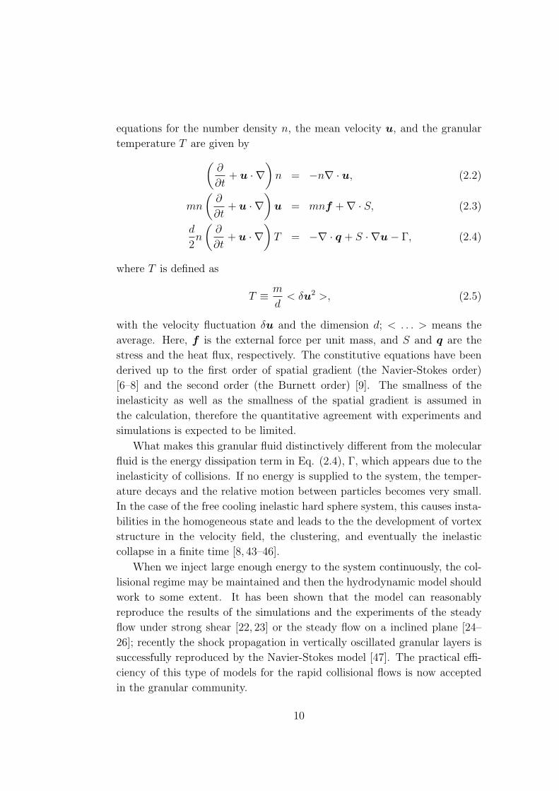
equations for the number density n, the mean velocity u, and the granular

temperature T are given by

(∂

∂t+ u · ∇

)n = −n∇ · u, (2.2)

mn

(∂

∂t+ u · ∇

)u = mnf +∇ · S, (2.3)

d

2n

(∂

∂t+ u · ∇

)T = −∇ · q + S · ∇u− Γ, (2.4)

where T is defined as

T ≡ m

d< δu2 >, (2.5)

with the velocity fluctuation δu and the dimension d; < . . . > means the

average. Here, f is the external force per unit mass, and S and q are the

stress and the heat flux, respectively. The constitutive equations have been

derived up to the first order of spatial gradient (the Navier-Stokes order)

[6–8] and the second order (the Burnett order) [9]. The smallness of the

inelasticity as well as the smallness of the spatial gradient is assumed in

the calculation, therefore the quantitative agreement with experiments and

simulations is expected to be limited.

What makes this granular fluid distinctively different from the molecular

fluid is the energy dissipation term in Eq. (2.4), Γ, which appears due to the

inelasticity of collisions. If no energy is supplied to the system, the temper-

ature decays and the relative motion between particles becomes very small.

In the case of the free cooling inelastic hard sphere system, this causes insta-

bilities in the homogeneous state and leads to the the development of vortex

structure in the velocity field, the clustering, and eventually the inelastic

collapse in a finite time [8, 43–46].

When we inject large enough energy to the system continuously, the col-

lisional regime may be maintained and then the hydrodynamic model should

work to some extent. It has been shown that the model can reasonably

reproduce the results of the simulations and the experiments of the steady

flow under strong shear [22, 23] or the steady flow on a inclined plane [24–

26]; recently the shock propagation in vertically oscillated granular layers is

successfully reproduced by the Navier-Stokes model [47]. The practical effi-

ciency of this type of models for the rapid collisional flows is now accepted

in the granular community.

10

The validity of a continuum description of granular materials, however,

has been questioned and remains as an open problem [2]. Even in the rapid

collisional flow, the Navier-Stokes model fails to describe the flow behavior at

very close to the boundary [26]. One of the reasons of this deviation should

be the spinning motion of each grain. It has been known that the mean spin

often deviates from the vorticity of the mean velocity near the boundary

[32, 48]. In addition, the angular momentum of the spinning motion is not

always negligible compared to that of the rotation of bulk velocity, because of

the macroscopic size of the particles. When we consider the grains with rough

surface or of arbitrarily shapes, it is possible that the coupling between the

particle spin and the mean velocity has some influence on the macroscopic

flow behavior.

The micropolar fluid model is a continuum model to describe a fluid

that consists of particles with spinning motion [27–30]. The angular velocity

field as well as the density and the velocity fields is considered in the model

equations, and an asymmetric stress tensor and a couple stress tensor are

included. Therefore, the model can be a suitable framework to describe

granular flows.

Some researches have been carried out to incorporate the spin into the

kinetic theory for granular materials to obtain the constitutive equations with

the effect of particle spin [49–51]. However, the effect of the couple stress

was neglected in most of them; when they solved the obtained hydrodynamic

equations, it has been assumed that the mean spin matches with the vorticity

of the mean velocity, and the deviation near the boundary was not considered.

In the meantime, the micropolar fluid model has been applied to dense

granular flows [52, 53]. However, the constitutive equations adopted for the

stress and the couple stress tensors were very complicated; it was difficult

to interpret the results physically. The application of the micropolar fluid

model with simple constitutive equations to the collisional flow will help us

to understand the effect of the particle spin in granular flow.

Another interesting issue on granular flow is its dynamical instability. In

most of the researches on rheology of collisional granular flow, the steady

uniform flow is considered. It is known, however, that uniform granular

flow often shows instabilities owing to the energy dissipation. The granular

flow on a slope often exhibits the coexistence of the collisional regime and

the frictional regime [4, 14, 54]. In the case of the shear flow of inelastic

particles, the formation of microstructure or small clusters has been observed

numerically [55]. The instability cause the density wave formation in the

11

granular flow in a vertical pipe where the power spectrum of the density

fluctuation obeys a power law [31, 56–60]. Recently, the wave formation

of granular flow on a slope has been found experimentally in rather low-

density flow [61] and in the dense flow [62]. It is important to investigate the

dynamical instability in rapid granular flow because the formation of dense

region may imply the breakdown of the collisional behavior.

2.3 Frictional Flow

When the injection of energy to the system is small, sustained contacts and

many-body collisions take place and the kinetic theory based on binary col-

lisions fails. Such a slow, dense, and frictional flow is widely found in real

systems under gravity.

One of the examples of the frictional flow found in our daily life is the flow

on the surface of a granular pile. When we observe the cross-section of the

surface flow, it is found that only thin layer of granular material is flowing

rapidly, and the width of the layer is the order of 10 diameters of grains

[1]. Komatsu et al. have shown in their experiment of steady flow on a

granular pile that the grains in the “frozen” bulk region, namely, the grains

below the rapidly flowing layer, exhibit creeping motion with the velocity

profile decaying exponentially [63]. The surface flow of granular material in

a rotating drum has been also investigated [64, 65]. In these surface flows,

the angle of the flowing surface is close to the angle of repose and the rapidly

flowing layer is thin; the angle and the depth of the flowing layer is determined

spontaneously.

For the flow on a solid plane, in contrast, both the inclination angle and

the flow depth can be controlled. In this geometry, the flow behavior strongly

depends on the roughness of the solid plane. When the flat bottom is used,

the high shear rate region is confined in the thin layer near the bottom, and

the bulk of material over that sheared layer slides down with very small shear

rate [62, 66]. In the case of rough bottom, the slip velocity at the boundary

becomes smaller, while the velocity profile depends very much on the height

of the flowing material and the inclination angle [67].

The cause of the complex behavior is the various types of interactions in

the dense granular flow; we should consider not only the inelastic collisions

but also the static and the dynamical friction force, and the effect of arching

or force chain. The excluded volume effect also plays an important role. At

12

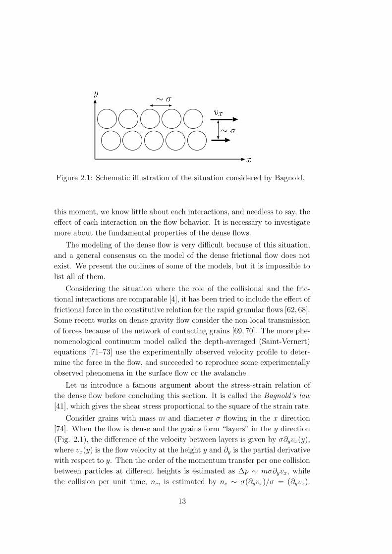
Figure 2.1: Schematic illustration of the situation considered by Bagnold.

this moment, we know little about each interactions, and needless to say, the

effect of each interaction on the flow behavior. It is necessary to investigate

more about the fundamental properties of the dense flows.

The modeling of the dense flow is very difficult because of this situation,

and a general consensus on the model of the dense frictional flow does not

exist. We present the outlines of some of the models, but it is impossible to

list all of them.

Considering the situation where the role of the collisional and the fric-

tional interactions are comparable [4], it has been tried to include the effect of

frictional force in the constitutive relation for the rapid granular flows [62, 68].

Some recent works on dense gravity flow consider the non-local transmission

of forces because of the network of contacting grains [69, 70]. The more phe-

nomenological continuum model called the depth-averaged (Saint-Vernert)

equations [71–73] use the experimentally observed velocity profile to deter-

mine the force in the flow, and succeeded to reproduce some experimentally

observed phenomena in the surface flow or the avalanche.

Let us introduce a famous argument about the stress-strain relation of

the dense flow before concluding this section. It is called the Bagnold’s law

[41], which gives the shear stress proportional to the square of the strain rate.

Consider grains with mass m and diameter σ flowing in the x direction

[74]. When the flow is dense and the grains form “layers” in the y direction

(Fig. 2.1), the difference of the velocity between layers is given by σ∂yvx(y),

where vx(y) is the flow velocity at the height y and ∂y is the partial derivative

with respect to y. Then the order of the momentum transfer per one collision

between particles at different heights is estimated as ∆p ∼ mσ∂yvx, while

the collision per unit time, nc, is estimated by nc ∼ σ(∂yvx)/σ = (∂yvx).

13

Therefore, the shear stress, Syx, is estimated as

Syx ∼ 1

σ2∆pnc ∼ m

σ(∂yvx)

2, (2.6)

which is the famous Bagnold’s law.

This law gives a simple scaling law between the total height of the flow h

and the flow velocity vx when it is applied to the steady flow on an inclined

plane with the inclination angle θ. The equation of motion in the x direction

is given by ρ(y)g sin θ + ∂ySyx = 0, where ρ is the mass density and g is

the acceleration of gravity. When the density is high and thus ρ can be

considered as a constant over the flow depth, it gives

Syx = ρg(h− y) sin θ, (2.7)

where h is the depth of the flowing material. From Eqs. (2.6) and (2.7), we

get

vx(y) = A[h3/2 − (h− y)3/2] (2.8)

when vx(0) = 0, with a constant A. Finally we obtain the scaling law

vx(h) = Ah3/2. (2.9)

A recent experiment on the dense flow down a rough slope performed

by Pouliquen revealed a simple scaling law of velocity [75]. He changed the

height of the flowing grains h and the inclination angle θ, and measured the

flow velocity u. He determined the line h = hstop(θ) in the θ vs. h plane,

below which the flow stops. This indicates the angle of repose depends on the

height of the flowing layer. Then he found that the flow velocity of different

θ or different material obeys the scaling law

u√gh

= βh

hstop(θ), (2.10)

with the acceleration of gravity g and a numerical constant β. This law can

be regarded as an extension of Eq. (2.9). Such a simple scaling is surprising

for those who are studying the physics of the dense granular flow, and is the

active topic of current study [67, 76, 77].

14

Chapter 3

Modeling of Interactions in

Granular Material

As emphasized in Chapter 1 and 2, the dissipative nature of the interactions

between gains makes them behave very differently from molecular systems.

Some simple phenomenological models with dissipative interactions have suc-

ceeded to reproduce the characteristic behaviors of granular material, though

the detail of interactions between grains such as the friction and the plas-

tic deformation are very complicated and still under discussion [11]. In this

chapter, we introduce two models which have been commonly used for the

simulations of granular dynamics; they are the soft sphere model called the

discrete element method (DEM) and the inelastic hard sphere model. The

correspondence of parameters between the two models is discussed in the last

section.

3.1 Discrete Element Method (DEM)

In the soft sphere model, which is sometimes called the discrete element

method (DEM) in the granular community [11, 13, 78], the particles overlap

during collision and the dynamics is defined through the forces acting on

the colliding particles. Collision takes finite time, thus not only the binary

collision but also the many-body collision and the sustained contact between

particles are possible; both the collisional and the frictional flows may realize

in the model. It is widely used for molecular dynamics simulations of granular

flow on a slope under gravity [14–19].

Here we introduce the two dimensional model with the linear elastic force

15

and dissipation. The extensions of the model to three dimension or to the

non-linear force law are found in Refs. [11, 78].

Let us consider the two disks i and j of the diameters σi and σj and the

masses mi and mj at the positions ri and rj with the velocities ci and cj

and the angular velocities ωi and ωj. If the particles are in contact, namely,

∆ ≡ σi + σj

2− |rij| > 0, (3.1)

where rij ≡ ri − rj, the force acting on the particle i from the particle j is

calculated as follows: The relative velocity of the point of contact vij is given

by

vij = (ci − cj) + n×(σi

2ωi +

σj

2ωj

), (3.2)

with the normal vector n = rij/|rij| = (nx, ny, 0). Then the normal veloc-

ity vn, the tangential velocity vt, and the tangential displacement ut at the

contact point are given by

vn = n · vij, vt = t · vij, (3.3)

ut =

∫ t

t0

vtdt, (3.4)

with t = (−ny, nx, 0). Here, t0 is the time when the two particles start to be

in contact. Then the normal force F ijn and the tangential force F ij

t acting on

the particle i from the particle j are given by

F ijn = 2Mkn∆− 2Mηnvn, (3.5)

F ijt = min(|hij

t |, µ|F ijn |)sign(hij

t ) (3.6)

with

hijt = −2Mktut − 2Mηtvt, (3.7)

where kn and kt are elastic constants, ηn and ηt are damping parameters,

and M = mimj/(mi + mj) is the reduced mass 1. µ is the Coulomb friction

coefficient for sliding. No force is applied between the particles i and j

when ∆ < 0. In the simulations, the equation of motion of each particle is

numerically integrated with a certain time step.

This phenomenological model simply expresses the normal and tangential

elastic force by linear springs, the dissipations by linear dashpots, and the

1The reason why we introduced the reduced mass here is to simplify the expressions ofthe correspondence of the DEM parameters to the parameters in the inelastic hard spheremodel. (See Section 3.3.)

16

(a)

kn

nη

(b)k

η

t

tµ

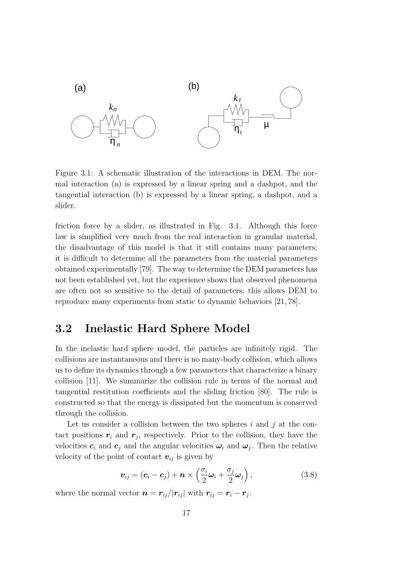
Figure 3.1: A schematic illustration of the interactions in DEM. The nor-

mal interaction (a) is expressed by a linear spring and a dashpot, and the

tangential interaction (b) is expressed by a linear spring, a dashpot, and a

slider.

friction force by a slider, as illustrated in Fig. 3.1. Although this force

law is simplified very much from the real interaction in granular material,

the disadvantage of this model is that it still contains many parameters;

it is difficult to determine all the parameters from the material parameters

obtained experimentally [79]. The way to determine the DEM parameters has

not been established yet, but the experience shows that observed phenomena

are often not so sensitive to the detail of parameters; this allows DEM to

reproduce many experiments from static to dynamic behaviors [21, 78].

3.2 Inelastic Hard Sphere Model

In the inelastic hard sphere model, the particles are infinitely rigid. The

collisions are instantaneous and there is no many-body collision, which allows

us to define its dynamics through a few parameters that characterize a binary

collision [11]. We summarize the collision rule in terms of the normal and

tangential restitution coefficients and the sliding friction [80]. The rule is

constructed so that the energy is dissipated but the momentum is conserved

through the collision.

Let us consider a collision between the two spheres i and j at the con-

tact positions ri and rj, respectively. Prior to the collision, they have the

velocities ci and cj and the angular velocities ωi and ωj. Then the relative

velocity of the point of contact vij is given by

vij = (ci − cj) + n×(σi

2ωi +

σj

2ωj

), (3.8)

where the normal vector n = rij/|rij| with rij = ri − rj.

17

ij

ci

cjn

J

vij

ωiωjγ

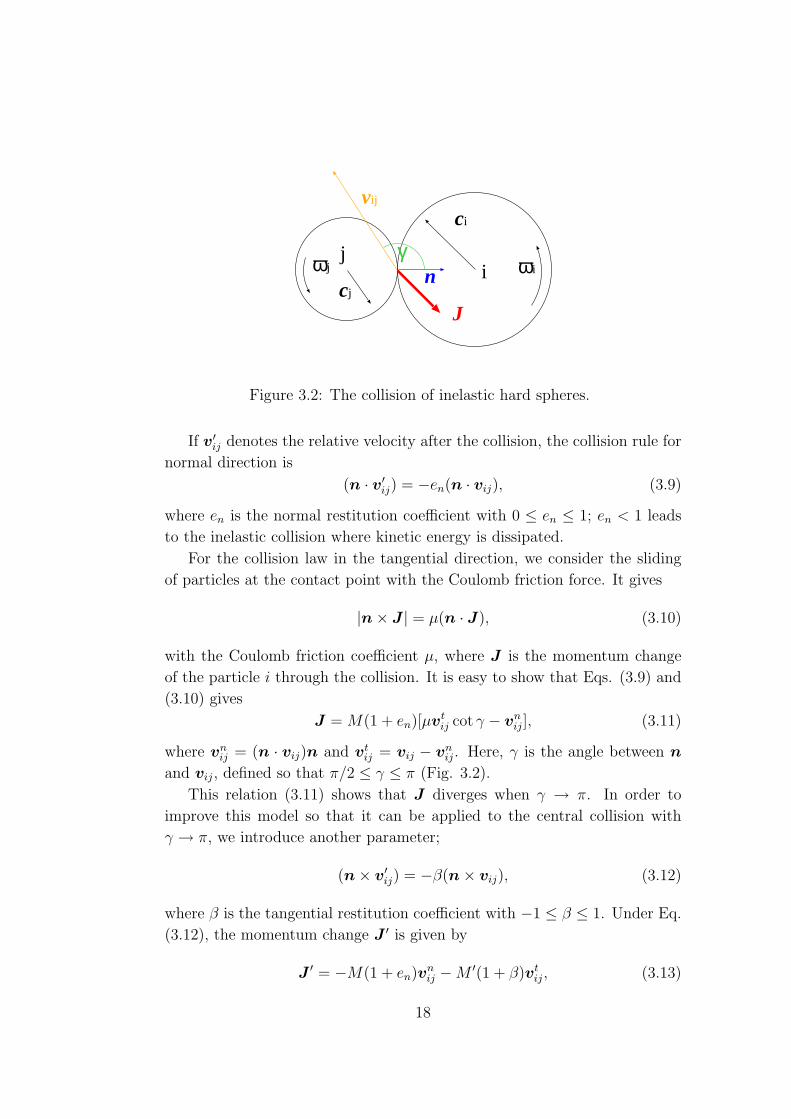
Figure 3.2: The collision of inelastic hard spheres.

If v′ij denotes the relative velocity after the collision, the collision rule for

normal direction is

(n · v′ij) = −en(n · vij), (3.9)

where en is the normal restitution coefficient with 0 ≤ en ≤ 1; en < 1 leads

to the inelastic collision where kinetic energy is dissipated.

For the collision law in the tangential direction, we consider the sliding

of particles at the contact point with the Coulomb friction force. It gives

|n× J | = µ(n · J), (3.10)

with the Coulomb friction coefficient µ, where J is the momentum change

of the particle i through the collision. It is easy to show that Eqs. (3.9) and

(3.10) gives

J = M(1 + en)[µvtij cot γ − vn

ij], (3.11)

where vnij = (n · vij)n and vt

ij = vij − vnij. Here, γ is the angle between n

and vij, defined so that π/2 ≤ γ ≤ π (Fig. 3.2).

This relation (3.11) shows that J diverges when γ → π. In order to

improve this model so that it can be applied to the central collision with

γ → π, we introduce another parameter;

(n× v′ij) = −β(n× vij), (3.12)

where β is the tangential restitution coefficient with −1 ≤ β ≤ 1. Under Eq.

(3.12), the momentum change J ′ is given by

J ′ = −M(1 + en)vnij −M ′(1 + β)vt

ij, (3.13)

18

with1

M ′ =1

M+

1

4

(σ2

i

Ii

+σ2

j

Ij

), (3.14)

where Ii is the moment of inertia of the particle i. For the two dimensional

disks with Ii = miσ2i /8, it gives M ′ = M/3.

The collision rule in the tangential direction depends on γ. The critical

value, γ0, which determine whether particles slide or not, is given by J = J ′,namely,

tan γ0 = −µM(1 + en)

M ′(1 + β). (3.15)

Equation (3.10) is applied when γ < γ0, and Eq. (3.12) is applied when

γ > γ0.

The collision of perfectly smooth particles corresponds to β = −1 and

µ = 0, because vtij does not change through the collision in this case. Such a

simple model with en < 1, namely, the model in which the energy dissipates

through the inelastic normal collision only, have been widely used to investi-

gate the fundamental properties of granular system [2, 43, 44, 46, 81, 82]. The

rule without the Coulomb friction which is characterized by en and β only is

also often used as a simple model with the particle rotation [8, 49, 51].

Because the collisions are instantaneous, the event-driven method is used

for numerical simulation of the inelastic hard sphere system. Very effec-

tive algorithms have been developed for the event-driven simulation of hard

sphere systems [12], which enables to simulate very large system.

The problem of the inelastic hard sphere model is that it cannot be used

for the situation where the sustained contact occurs. It is known that the

system often shows the singular behavior which is called inelastic collapse,

namely, the infinite number of collision among a small number of particle

within a finite time [2] 2 ; the dynamics cannot go beyond this point without

additional assumption. Therefore, the situations where the inelastic hard

sphere model is applicable are rather limited.

3.3 Correspondence of Parameters between

the Models

One of the advantages of the inelastic hard sphere model to DEM is its

simplicity; parameters in the former is fewer than those in the latter. When

2The more description of the inelastic collapse is given in Section 4.2.

19

we adopt the linear dependence of the elastic and viscous force on the overlap

∆ and the relative velocity, respectively, we can relate the parameters in DEM

to those in the inelastic hard sphere model [83]. In the following, we briefly

summarize the correspondence of the parameters.

Suppose that the particle i at ri(t) = (xi(t), 0) and the particle j at

rj(t) = (xj(t), 0) collide at t = 0 with the relative velocity rj(0) − ri(0) =

(−v0, 0), where the dots represent the time derivatives. The overlap of the

two particles is ∆(t) = (σi+σj)/2−(xi(t)−xj(t)) and the equation of motion

for ∆(t) becomes

∆ = xj − xi

= −2ηn∆− 2kn∆, (3.16)

from Eq. (3.5). With the initial conditions ∆(0) = 0 and ∆(0) = v0 > 0, we

get

∆(t) =v0√

2kn − η2n

exp (−ηnt) sin(√

2kn − η2nt

). (3.17)

The collision ends when ∆(t) = 0, thus the duration of the contact τc and

and the normal restitution coefficient en are given by

τc =π√

2kn − η2n

(3.18)

and

en = exp

(− πηn√

2kn − η2n

), (3.19)

respectively. 3

The similar relations can be obtained for the binary collision with non-

zero tangential relative velocity. Neglecting the Coulomb friction and n

during the contact, 4 the equation for the tangential displacement ut(t) is

written in the following form [83];

ut = −(2ktut + 2ηtut)M

M ′ (3.20)

3This relation holds for the normal collision only; otherwise we need to take into accountthe variation of the normal vector n for the calculation of ∆(t). In the hard sphere limitof kn →∞ (see Section 4.1), however, we can neglect the variation n during the collision,and the expression (3.19) corresponds to en in the hard sphere model.

4The variation of n during the collision becomes negligible in the hard sphere limit, asdenoted above.

20

where M ′ is given in Eq. (3.14). Therefore, a half period of the tangential

oscillation is given by

τs =π√

6kt − 9η2t

(3.21)

for two dimensional disks with moment of inertia Ii = miσ2i /8. Here we

choose the parameters kt and ηt so that the relation τs = τc is satisfied:√

6kt − 9η2t =

√2kn − η2

n. (3.22)

Under this condition, the tangential restitution coefficient is given by

β = exp(−3ηtτc). (3.23)

Now we have the expressions of all the parameters in the collision rule of the

inelastic hard sphere model: en, β, and µ. When the parameters are chosen

so that these relations hold, the only additional parameter in DEM is kn,

which determines the duration of contact τc.

Though it is known that the restitution coefficients are not simple con-

stants in real material and depends on the relative velocity and the collision

angle [84, 85], they are often given in the literature of the experiments of

granular material. One possible way to determine the DEM parameters may

be to use these relations to obtain the desired restitution coefficients. It

should be questioned, however, whether the force suitable for the collisional

events describes the frictional force in the sustained contact properly.

How can we determine the duration of contact τc? In general τc depends

on the detail of the collision, but the order of τc may be estimated by the

theory of elasticity. The elastic energy Ue stored by two identical three-

dimensional spheres deformed over the depth ∆ is derived by Hertz [11, 86],

which is given by

Ue =1

2k∆5/2, (3.24)

with

k =4

15

E

1− ν2

√σ, (3.25)

where E and ν are Young’s modulus and Poisson’s coefficient, respectively 5.

Therefore, when the relative velocity of the spheres at the moment of contact

is v0, the energy conservation law reads

1

2Mv2

0 =1

2k∆5/2 +

1

2M∆2. (3.26)

5The Hertz’s theory gives the elastic force proportional to ∆3/2. The DEM with theelastic force of this non-linear dependence on ∆ is also widely used.

21

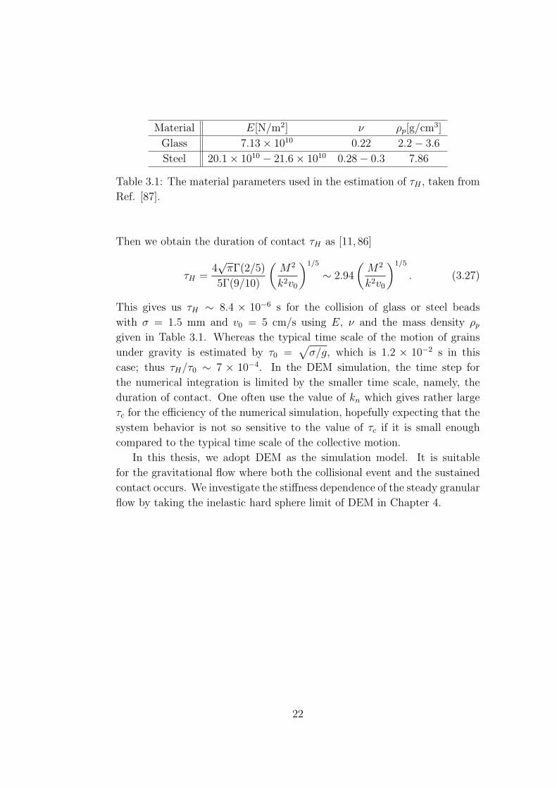
Material E[N/m2] ν ρp[g/cm3]

Glass 7.13× 1010 0.22 2.2− 3.6

Steel 20.1× 1010 − 21.6× 1010 0.28− 0.3 7.86

Table 3.1: The material parameters used in the estimation of τH , taken from

Ref. [87].

Then we obtain the duration of contact τH as [11, 86]

τH =4√

πΓ(2/5)

5Γ(9/10)

(M2

k2v0

)1/5

∼ 2.94

(M2

k2v0

)1/5

. (3.27)

This gives us τH ∼ 8.4 × 10−6 s for the collision of glass or steel beads

with σ = 1.5 mm and v0 = 5 cm/s using E, ν and the mass density ρp

given in Table 3.1. Whereas the typical time scale of the motion of grains

under gravity is estimated by τ0 =√

σ/g, which is 1.2 × 10−2 s in this

case; thus τH/τ0 ∼ 7 × 10−4. In the DEM simulation, the time step for

the numerical integration is limited by the smaller time scale, namely, the

duration of contact. One often use the value of kn which gives rather large

τc for the efficiency of the numerical simulation, hopefully expecting that the

system behavior is not so sensitive to the value of τc if it is small enough

compared to the typical time scale of the collective motion.

In this thesis, we adopt DEM as the simulation model. It is suitable

for the gravitational flow where both the collisional event and the sustained

contact occurs. We investigate the stiffness dependence of the steady granular

flow by taking the inelastic hard sphere limit of DEM in Chapter 4.

22

Chapter 4

Hard Sphere Limit of DEM:

Stiffness Dependence of Steady

Granular Flows

The granular flows are classified into two types as has been described in

Chapter 1 and 2, i.e., the collisional flow and the frictional flow, depending

on the dominant interaction; the former is dominated by the inelastic collision

and the latter is dominated by the sustained contact.

For the simulation of granular flow, the models introduced in Chapter

3, the soft sphere model (DEM) and the inelastic hard sphere model, are

commonly used.

The inelastic hard sphere model is effective to investigate the fundamental

properties of collisional granular flow thanks to its simplicity. However, it

cannot be used for the frictional flow, because the sustained contact is not

allowed. It is also known that the system often encounters the inelastic

collapse.

The both flows may realize in DEM. However, the stiffness parameter

used in DEM is often much smaller than the one appropriate for the real

materials like steel or glass ball. It is also not clear that the frictional force

in the sustained contact may be described by the same forces with the one

suitable for the collisional events. Therefore, it is important to examine

how the system behavior changes upon increasing the stiffness of particles

with keeping the restitution constant unchanged, or taking the inelastic hard

sphere limit of DEM.

In this chapter, we numerically investigate how the behavior of the col-

23

lisional flow and the frictional flow change on taking the hard sphere limit

of DEM. In Section 4.1, we summarize how we take the hard sphere limit

keeping the restitution coefficient constant; we use the correspondence of

parameters given in Section 3.3. Then we discuss the limiting behavior in

some simple situations where the hard sphere model results in the inelas-

tic collapse in Section 4.2. In Section 4.3, the simulation results are shown.

At first, the stiffness dependence of the steady motion of a single particle

rolling down a slope is presented to see how the inelastic collapse appears in

the hard sphere limit. Then, the collisional flow and the frictional flow are

examined. We find that the interactions between particles in the collisional

flow smoothly converge to binary collisions of inelastic hard spheres, while

those in frictional flow shows non-trivial behavior; the behavior is also differ-

ent from the “inelastic collapse” in the single particle system. The summary

and the discussion are given in Section 4.4.

4.1 Hard sphere Limit of DEM

We summarize how we take the hard sphere limit using the correspondence

of parameters.

The binary collision rule in the inelastic hard sphere model in Section

3.2 is determined by the normal restitution constant en (Eq. (3.9)), the

tangential restitution constant β (Eq. (3.12)), and the Coulomb friction

coefficient µ (Eq. (3.10)). In DEM, the force acting on the colliding particle

is determined by the normal stiffness constant kn and the damping parameter

ηn (Eq. (3.5)), the tangential stiffness constant kt and the damping parameter

ηt (Eq. (3.7)), and the Coulomb friction coefficient µ (Eq. (3.6)).

In Section 3.3, the following relations are shown: The duration of contact

τc for a normal binary collision and the normal restitution coefficient en

in DEM are given in Eqs. (3.18) and (3.19), respectively. The tangential

restitution coefficient β is given by Eq. (3.23) under the condition (3.22).

Equations (3.18) and (3.19) can be rewritten as

ηn =

[2kn

(π/ ln en)2 + 1

]1/2

, (4.1)

τc =

[π2 + (ln en)2

2kn

]1/2

. (4.2)

Using these relations, we can take the inelastic hard sphere limit of this model

for given restitution coefficients en and β by taking the kn → ∞ limit; ηn,

24

ηt, and kt are given by Eqs. (4.1), (3.23), and (3.22), and the duration time

of collision τc goes to zero as Eq. (4.2).

4.2 Inelastic Collapse

It is well known that the inelastic hard sphere system can undergo inelastic

collapse, the phenomenon where infinite collisions take place within a finite

period of time [2]. A simple example is the vertical bouncing motion of a ball

under gravity. When the collision between the floor and the ball is inelastic,

the velocity of the ball just before the nth collision vn and the next one have

the relation

vn+1 = ewvn (4.3)

with 0 ≤ ew < 1; the ball undergoes the infinite number of collision within

the period 2v0/[g(1− ew)].

The inelastic collapse also occurs without gravity. The simplest example

is three inelastic balls in one dimension, and a ball goes back and forth

between the other two approaching each other; the three balls lose relative

velocity completely in the limit of infinite collisions [88, 89]. The inelastic

collapse has been also found in the event-driven simulations of free cooling

inelastic hard sphere system in higher dimension [90, 91]. Furthermore, it

has been recently reported that the inelastic collapse occurs even in the

shear flow, although it is natural to think that the shear tends to prevent the

collapse [92].

The inelastic collapse never occurs in the soft sphere model. However, it

is worth to discuss what will happen in the soft sphere model in a simple

situation where the inelastic collapse occurs in the hard sphere model.

Let us consider the vertical bouncing motion of a soft ball under gravity

at first. We assume the same force law between the ball and the floor as in

Eqs. (3.5) and (3.6), except that we replace 2M by the mass of the ball m.

When the ball and the floor are in contact, the equation of motion for the

overlap of the ball and the floor, z, is given by

z + knz + ηnz = g. (4.4)

Therefore, when the velocity just before the collision is small enough, the ball

cannot take off from the floor, and finally reaches the steady state of keeping

contact, z = g/kn > 0. One can show that, if the impact velocity vi is below

a critical value vc, which is O(1/√

kn) for large enough kn (Appendix B), the

25

ball stays in contact with the floor; for vi À vc, the restitution coefficient

ew defined in Eq. (4.3) can be considered as a constant. Therefore, for a

given initial impact velocity v0, the number of necessary collisions nc for the

ball to stay in contact with the floor is roughly estimated by the condition

encw v0 ∼ vc, namely, nc ∼ log (vc/v0) / log ew. Because vc ∼ 1/

√kn for large

kn, nc behaves as

nc ∝ log kn + const. (4.5)

in the hard sphere limit. Thus nc diverges logarithmically when kn → ∞,

which correspond to the inelastic collapse due to gravity.

In the case without gravity, the inelastic collapse results in the “many-

body collision” in the soft sphere model. For example, when we consider three

soft spheres in one dimension, the binary collision can be approximated by

the collision law with a constant restitution coefficient. However, when the

interval between two collisions becomes smaller than the duration of contact

τc, the three balls are in contact at the same time, namely, the three-body

collision occurs. They still have some relative motion, thus they will fly apart

after that. The number of collisions before the three-body collision will also

diverge logarithmically in the hard sphere limit because τc ∝ 1/√

kn.

One should note that a many-body collision in the soft sphere model

does not necessarily result in the inelastic collapse in the hard sphere limit.

Actually, in most of the cases, a many-body collision will be decomposed into

a set of binary collisions in the hard sphere limit.

4.3 Simulation Results

In this section, we investigate the stiffness dependence of granular material

on a slope in the following three situations: (i) a single particle rolling down

a slope, (ii) the dilute collisional flow, and (iii) the dense frictional flow. We

focus on the steady state in each situation and compare the simulation data

with changing kn systematically. The particles are monodisperse in (ii), while

they are polydisperse in (iii) in order to avoid crystallization.

In the simulations, the parameters have been chosen to give en = β = 0.7,

µ = 0.5 in the hard sphere limit. Each particle is also subject to the gravity,

and the gravitational acceleration is given by g = g(sin θ,− cos θ). All values

are non-dimensionalized by the length unit σ, the mass unit m, and the time

unit√

σ/g. Here, σ is the diameter of the largest particle in the system and

m is the mass of that particle. The second order Adams-Bashforth method

26

and the trapezoidal rule are used to integrate the equations for the velocity

and the position, respectively [93]. Note that the time step for integration,

dt, needs to be adjusted as τc becomes smaller. All the data presented in this

chapter are results with dt = min(τc/100, 10−4). We have confirmed that the

results do not change for dt ≤ τc/100 by calculating also with dt = τc/50 and

dt = τc/200 in the case of the single particle.

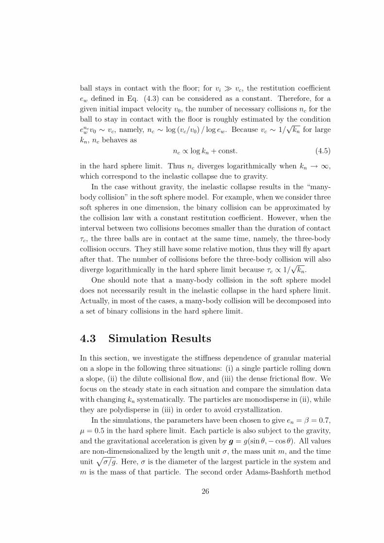
4.3.1 A single particle rolling down a bumpy slope

Figure 4.1: A snapshot of a single ball rolling down a rough slope.

Let us first consider a single particle rolling down a bumpy slope which

has been referred in Section 2.1. In the simulations, we make the boundary

rough by attaching the same particles with the rolling one to the slope with

the spacing 0.002σ (see Fig. 4.1). For the chosen parameters with the normal

stiffness kn = 2−1 × 105, the range of θ for which steady motion is realized

is 0.11 . sin θ . 0.14 (see Section 6.2). Here we fix the inclination angle

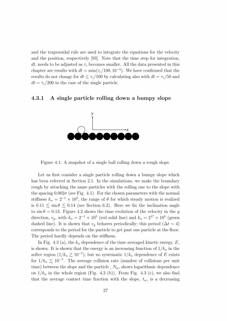
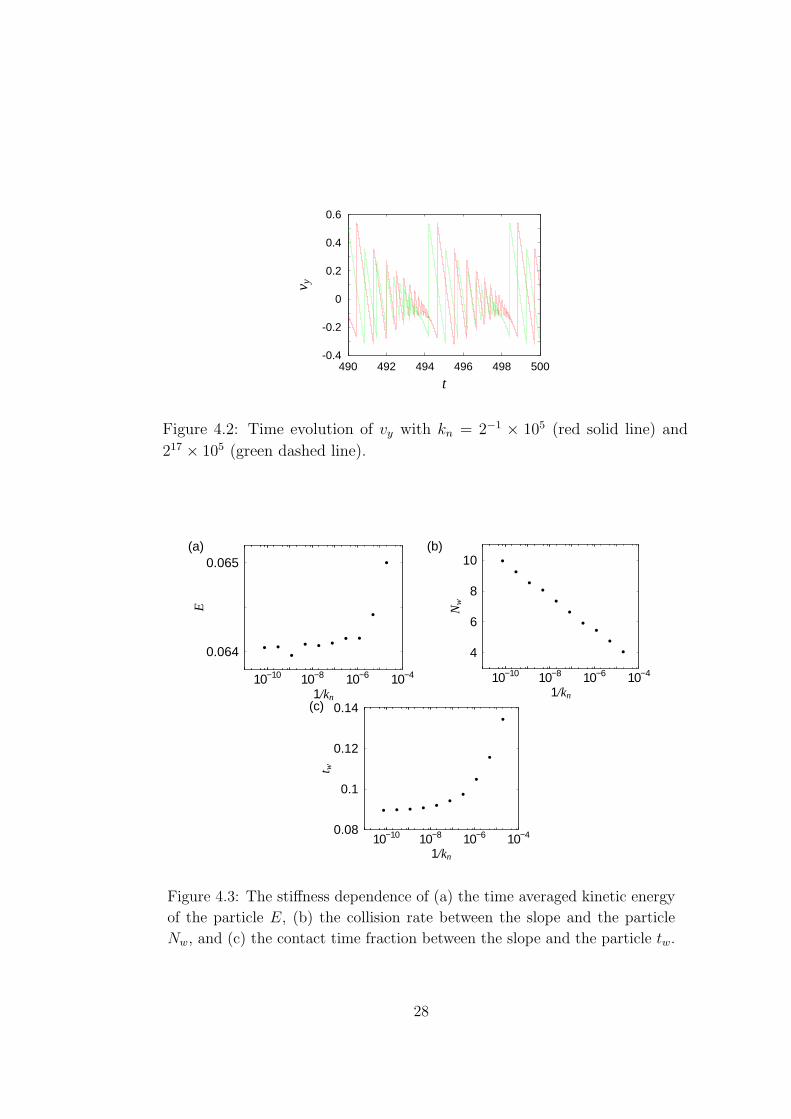
to sin θ = 0.13. Figure 4.2 shows the time evolution of the velocity in the y

direction, vy, with kn = 2−1 × 105 (red solid line) and kn = 217 × 105 (green

dashed line). It is shown that vy behaves periodically; this period (∆t ∼ 4)

corresponds to the period for the particle to get past one particle at the floor.

The period hardly depends on the stiffness.

In Fig. 4.3 (a), the kn dependence of the time averaged kinetic energy, E,

is shown. It is shown that the energy is an increasing function of 1/kn in the

softer region (1/kn & 10−7), but no systematic 1/kn dependence of E exists

for 1/kn . 10−7. The average collision rate (number of collisions per unit

time) between the slope and the particle , Nw, shows logarithmic dependence

on 1/kn in the whole region (Fig. 4.3 (b)). From Fig. 4.3 (c), we also find

that the average contact time fraction with the slope, tw, is a decreasing

27

-0.4

-0.2

0

0.2

0.4

0.6

490 492 494 496 498 500

v y

t

Figure 4.2: Time evolution of vy with kn = 2−1 × 105 (red solid line) and

217 × 105 (green dashed line).

(a)

0.064

0.065

10−10 10−8 10−6 10−4

E

1/kn

(b)

4

6

8

10

10−10 10−8 10−6 10−4

Nw

1/kn(c)

0.08

0.1

0.12

0.14

10−10 10−8 10−6 10−4

t w

1/kn

Figure 4.3: The stiffness dependence of (a) the time averaged kinetic energy

of the particle E, (b) the collision rate between the slope and the particle

Nw, and (c) the contact time fraction between the slope and the particle tw.

28

function of kn in the soft region, but it seems to approach a constant value

for large enough kn.

The logarithmic kn dependences of Nw and the constant tw in large kn

region agree with our previous analysis of “inelastic collapse under gravity”

in the soft sphere model in Section 4.2. The motion of the particle in one

period is as follows; when the particle comes to a bump (a particle attached

to the slope), the particle jumps up, bounces on the bump many times, loses

the relative velocity, and finally rolls down keeping in contact with the bump.

Therefore, the contact time fraction has a finite value even in the hard sphere

limit due to the rolling motion at the last part. Nw increases logarithmically

in the hard sphere limit as has been expected from Eq. (4.5).

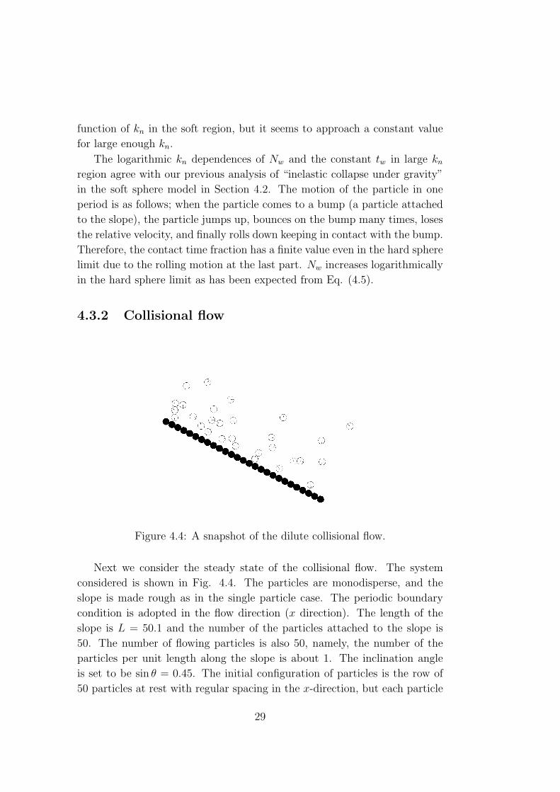
4.3.2 Collisional flow

Figure 4.4: A snapshot of the dilute collisional flow.

Next we consider the steady state of the collisional flow. The system

considered is shown in Fig. 4.4. The particles are monodisperse, and the

slope is made rough as in the single particle case. The periodic boundary

condition is adopted in the flow direction (x direction). The length of the

slope is L = 50.1 and the number of the particles attached to the slope is

50. The number of flowing particles is also 50, namely, the number of the

particles per unit length along the slope is about 1. The inclination angle

is set to be sin θ = 0.45. The initial configuration of particles is the row of

50 particles at rest with regular spacing in the x-direction, but each particle

29

(a)

0

10

20

30

10−8 10−6 10−4 10−2

E

1/kn

(b)

0

0.5

1.0

10−8 10−6 10−4 10−2

Nc

, N

w

1/kn

(c)

10−5

10−4

10−3

10−2

10−1

10−8 10−6 10−4 10−2

t c ,

t w

1/kn

(d)

-0.01

-0.005

0

10−8 10−6 10−4 10−2

t c−N

cτc

, t

w−N

wτ w

1/kn

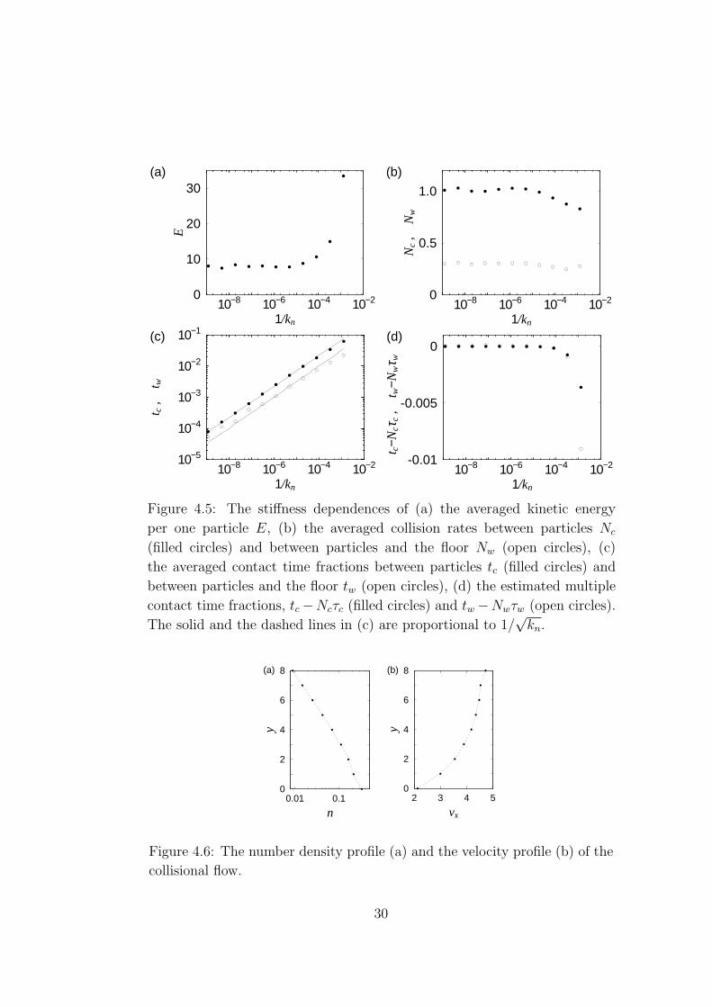
Figure 4.5: The stiffness dependences of (a) the averaged kinetic energy

per one particle E, (b) the averaged collision rates between particles Nc

(filled circles) and between particles and the floor Nw (open circles), (c)

the averaged contact time fractions between particles tc (filled circles) and

between particles and the floor tw (open circles), (d) the estimated multiple

contact time fractions, tc−Ncτc (filled circles) and tw−Nwτw (open circles).

The solid and the dashed lines in (c) are proportional to 1/√

kn.

(a)

0

2

4

6

8

0.01 0.1

y

n

(b)

0

2

4

6

8

2 3 4 5

y

vx

Figure 4.6: The number density profile (a) and the velocity profile (b) of the

collisional flow.

30

is at random height in the y-direction. After a short initial transient, if the

total kinetic energy fluctuates around a certain value, we consider it as the

steady flow. All the data were taken in this regime and averaged over the

time period of 1500.

As can be seen in the snapshot, Fig. 4.4, the particles bounce and the

number of particles in contact is very small. In Fig. 4.5 (a), the averaged

kinetic energy per one particle, E, is shown. Though E becomes larger as

the particles become softer in 1/kn & 10−5, the systematic dependence of E

on kn disappears for large enough kn (1/kn . 10−6). 1 The y-dependence of

the average number density and the flow speed in this region are also shown

in Fig. 4.6 (a) and (b).

In Fig. 4.5 (b), the average collision rates between particles, Nc (filled

circles), and between particles and the slope, Nw (open circles), per particle

are plotted v.s. 1/kn. Both of them stay roughly constant in the region where

E is almost constant, 1/kn . 10−6. The average time fractions during which

a particle is in contact with other particles, tc (filled circles), and in contact

with the slope, tw (open circles), decrease systematically as kn increases as

shown in Fig. 4.5 (c). Both the solid and the dashed lines are proportional to

1/√

kn, namely, tc decreases in the same manner as τc in Eq. (4.2). Actually,

the collision time fractions tc and tw converge to Ncτc and Nwτw (τw is the

duration of a normal collision of a particle and the floor), 2 respectively, in

the hard sphere limit. The differences tc − Ncτc and tw − Nwτw are plotted

in Fig. 4.5 (d) to show that they go to zero very rapidly upon increasing kn.

This means that the interactions of the soft sphere model in the collisional

flow regime converge to those of the inelastic hard sphere model with binary

collisions.

If we look carefully, however, in the large kn region in Fig. 4.5 (c), we

1The stiffness dependence of the motion of particles discharging from a hopper usingdiscrete element method has been studied by Yuu et al [20]. They performed the sim-ulations with three different values of stiffness and found the different behaviors. Thecomparison with the present results is not simple because of the different set up, but if wenormalize their parameter of normal stiffness with the particle mass, the diameter, andthe acceleration of gravity, then their values extend over the range where E depends onkn in our simulations.

2When we fix a particle on the slope and employ the same force law as Eq. (3.5), then wehave the duration of contact for the normal collision without gravity τw = π/

√kn − η2

n/4for identical particles. The force law for the flat boundary that replace 2M in Eq. (3.5)by the mass of the colliding particle m gives the same duration of contact with the aboveone for the normal collision (cf. Appendix B).

31

can see slight deviation of tw from the dashed line; it decreases slower than

1/√

kn. This tendency may indicate that tw remains finite in the hard sphere

limit: Actually, in the event-driven simulation of the hard sphere model, we

always found the inelastic collapse as long as the restitution constant between

a particle and the floor is less than 1. This suggests that Nw should diverge

and tw should remain finite in the hard sphere limit because of the inelastic

collapse due to gravity. The slight deviation of tw from the dashed line in

Fig. 4.5 (c) may be a symptom of it, while we cannot see the logarithmic

divergence in Nw.

4.3.3 Frictional flow

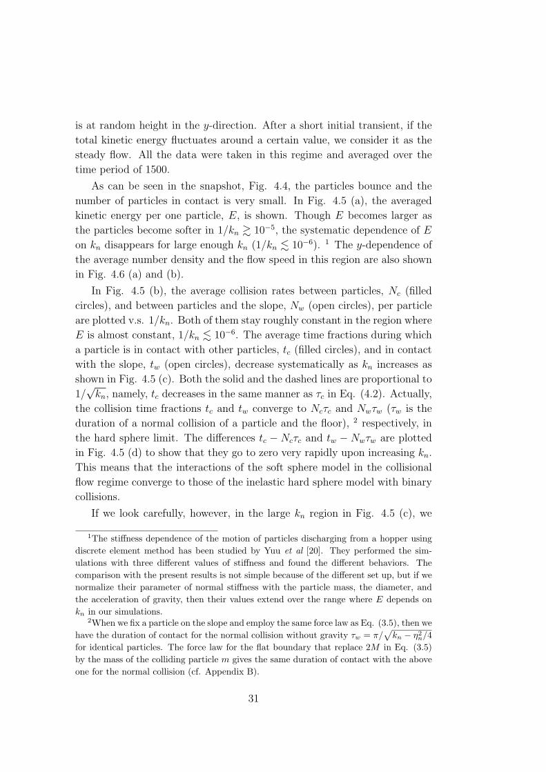
Figure 4.7: A snapshot of the dense frictional flow.

Now we study the steady state of the dense frictional flow. We adopt

the flat boundary with slope length L = 10.02 and imposed the periodic

boundary condition in the flow direction. In order to avoid crystallization,

we used the polydisperse particles with the uniform distribution of diameter

from 0.8 to 1.0. The number of particles in the system is 100. The inclination

angle θ is set to be sin θ = 0.20 and the initial condition is given in the similar

way with the collisional flow. The ten rows of ten particles with regular

spacing in the x-direction are at rest with large enough spacings between

rows in the y-direction so that particles do not overlap; only the particles in

the top row are at random heights in y-direction.

32

(a)

0

10

20

0 1000 2000

E(t)

t

sample 3

sample 1, sample 2

(b)

0.0

1.0

2.0

0 1000 2000E

(t)t

sample 3

sample 1

sample 2

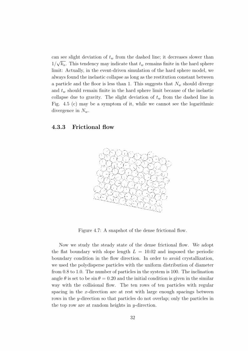
Figure 4.8: Time evolution of the kinetic energy per particle of three samples

(sample 1: red solid line, sample 2: green dashed line, sample 3: blue dotted

line). (b) is the magnification of (a). Sample 1 with kn = 2−1 × 105 shows

steady behavior within the threshold. Sample 2 and 3 are with kn = 2−7×105.

Sample 2 shows steady behavior with lower energy for a while but finally

stops. E(t) of sample 3 shoots up suddenly at t ∼ 1300 when one of the

particles in the bottom layer runs on other particles.

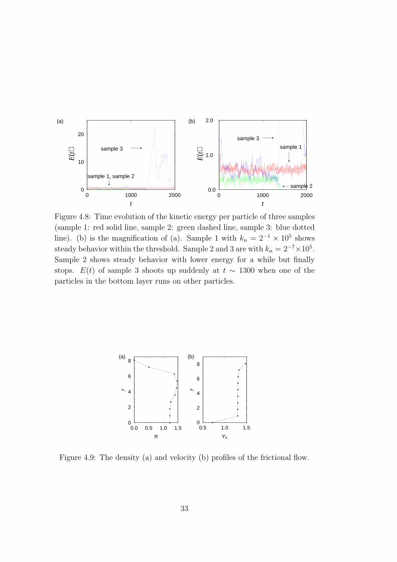
(a)

0

2

4

6

8

0.0 0.5 1.0 1.5

y

n

(b)

0

2

4

6

8

0.5 1.0 1.5

y

vx

Figure 4.9: The density (a) and velocity (b) profiles of the frictional flow.

33

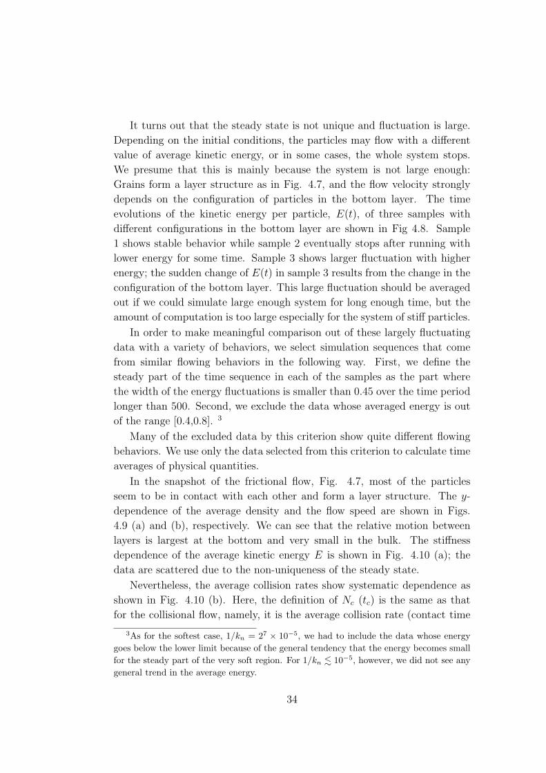
It turns out that the steady state is not unique and fluctuation is large.

Depending on the initial conditions, the particles may flow with a different

value of average kinetic energy, or in some cases, the whole system stops.

We presume that this is mainly because the system is not large enough:

Grains form a layer structure as in Fig. 4.7, and the flow velocity strongly

depends on the configuration of particles in the bottom layer. The time

evolutions of the kinetic energy per particle, E(t), of three samples with

different configurations in the bottom layer are shown in Fig 4.8. Sample

1 shows stable behavior while sample 2 eventually stops after running with

lower energy for some time. Sample 3 shows larger fluctuation with higher

energy; the sudden change of E(t) in sample 3 results from the change in the

configuration of the bottom layer. This large fluctuation should be averaged

out if we could simulate large enough system for long enough time, but the

amount of computation is too large especially for the system of stiff particles.

In order to make meaningful comparison out of these largely fluctuating

data with a variety of behaviors, we select simulation sequences that come

from similar flowing behaviors in the following way. First, we define the

steady part of the time sequence in each of the samples as the part where

the width of the energy fluctuations is smaller than 0.45 over the time period

longer than 500. Second, we exclude the data whose averaged energy is out

of the range [0.4,0.8]. 3

Many of the excluded data by this criterion show quite different flowing

behaviors. We use only the data selected from this criterion to calculate time

averages of physical quantities.

In the snapshot of the frictional flow, Fig. 4.7, most of the particles

seem to be in contact with each other and form a layer structure. The y-

dependence of the average density and the flow speed are shown in Figs.

4.9 (a) and (b), respectively. We can see that the relative motion between

layers is largest at the bottom and very small in the bulk. The stiffness

dependence of the average kinetic energy E is shown in Fig. 4.10 (a); the

data are scattered due to the non-uniqueness of the steady state.

Nevertheless, the average collision rates show systematic dependence as

shown in Fig. 4.10 (b). Here, the definition of Nc (tc) is the same as that

for the collisional flow, namely, it is the average collision rate (contact time

3As for the softest case, 1/kn = 27 × 10−5, we had to include the data whose energygoes below the lower limit because of the general tendency that the energy becomes smallfor the steady part of the very soft region. For 1/kn . 10−5, however, we did not see anygeneral trend in the average energy.

34

(a)

0

0.2

0.4

0.6

0.8

1.0

10−8 10−6 10−4 10−2

E

1/kn

(b)

1

10

100

1000

10000

10−8 10−6 10−4 10−2

Nc

, N

w

1/kn

∝kn0.4

(c)

0.1

1

10−8 10−6 10−4 10−2

t c ,

t w

1/kn

(d)

0

0.2

0.4

0.6

10−8 10−6 10−4 10−2

t c−N

cτc

, t

w−N

wτ w

1/kn

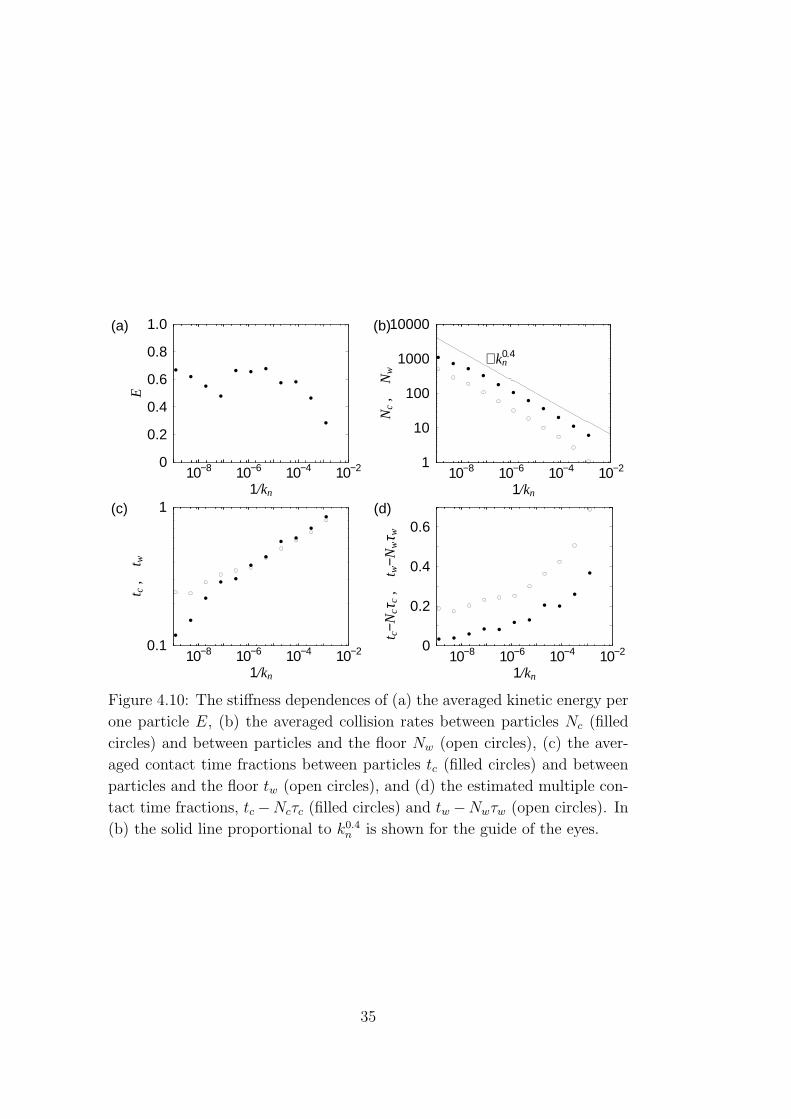
Figure 4.10: The stiffness dependences of (a) the averaged kinetic energy per

one particle E, (b) the averaged collision rates between particles Nc (filled

circles) and between particles and the floor Nw (open circles), (c) the aver-

aged contact time fractions between particles tc (filled circles) and between

particles and the floor tw (open circles), and (d) the estimated multiple con-

tact time fractions, tc−Ncτc (filled circles) and tw −Nwτw (open circles). In

(b) the solid line proportional to k0.4n is shown for the guide of the eyes.

35

fraction) between particles per particle in the system. Nw (tw) is defined

differently; it is the collision rate (the contact time fraction) between the

particles and the slope per particle in the bottom layer, because other particles

never touch the slope.

In Fig. 4.10 (b), we can see that Nc (filled circles) and Nw (open circles)

increase very rapidly as kn becomes larger: they diverge as a power of kn.

This is quite different from the behavior in the collisional flow in which they

are almost constant. Furthermore, this increase is faster than the logarithmic

divergence found in the single particle case (see Fig. 4.3 (b)).

The contact time fractions, tc (filled circles) and tw (open circles), decrease

as shown in Fig. 4.10 (c). The main reason why tc and tw decrease is that τc

and τw decrease faster than Nc and Nw, namely, the contact time fractions

estimated from the duration of a binary collision, Ncτc and Nwτw, continue to

decrease. Actually, the decrease of the contact time fraction and the increase

of the collision rate are natural because a longer multiple contact breaks up

into shorter binary contacts as the particles become stiffer.

These contact time fractions, tc and tw, however, do not converge to Ncτc

and Nwτw, respectively. As shown in Fig. 4.10 (d), tc − Ncτc (filled circles)

and tw − Nwτw (open circles) are very large as compared to those in the

collisional flow, even in the stiffest region. The comparison of this with the

rapid convergence in the collisional flow regime (Fig. 4.5 (d)) indicates that

there remains finite multiple contact time in the hard sphere limit and the

interaction in the frictional flow can never be considered as many, or even

infinite, instantaneous binary collisions. The particles experience the lasting

multiple contact even in the hard sphere limit.

4.4 Summary

The inelastic hard sphere limit of granular flow has been investigated numer-

ically in the steady states of (i) a single particle rolling down the slope, (ii)

the dilute collisional flow, and (iii) the dense frictional flow. In (i), it has

been found that the “inelastic collapse” between the particle and the slope

occurs in the hard sphere limit due to gravity, and the contact time frac-

tion between the particle and the slope remains finite. In (ii), the collision

rates, Nc and Nw, are almost constant when particles are stiff enough. The

contact time fraction between particles tc approaches zero as kn increase in

the same manner with the duration of contact for a binary collision τc. This

36

means that the interaction between particles in the hard sphere limit can be

expressed by binary collisions in the inelastic hard sphere model. However,

the decrease in tw is slightly slower than 1/√

kn in the harder region, which

can be a sign of the inelastic collapse between a particle and the slope.

In the case of the frictional flow (iii), the situation is not simple; Although

the contact time fractions tc and tw decrease upon increasing kn, the collision

rates Nc and Nw increase as a power of kn, which is faster than the logarithmic

divergence found in the single particle case (i). The origin of this power

divergence of collision rate does not seem to be simple because it is a property

of the steady state, not a particular dynamical trajectory of the system.

The multiple contact time fraction may be estimated by tc − Ncτc and

tw − Nwτw. They were found to be quite large compared to those for the

collisional flow, and seems to remain finite even in the infinite stiffness limit;

this suggests that the interaction in the frictional flow can never be considered

as infinite number of binary collisions. Even in the hard sphere limit, particles

experience the lasting multiple contact.

The non-negligible fraction of multiple contact in the hard sphere limit

implies the existence of the network of contacting grains even though they

are flowing [94]. The models for dense flow should consider the effect of these

lasting contacts.

Here we have investigated only the two cases, i.e., the collisional flow and

the frictional flow. The system should undergo the transition between the

two flows if we change continuously the parameters such as the inclination

angle, the roughness of the slope, or the density of particles. It is interesting

to investigate how the transition occurs by looking at the quantities measured

in this chapter, because their stiffness dependences are qualitatively different

in the two flows.

37

Chapter 5

Collisional Granular Flow as a

Micropolar Fluid: Effect of

Rotation of Grains

In spite of the long history of research on the granular flows, the theoreti-

cal framework for their rheology has not yet been established as stated in

Chapter 2. One reason that makes analytical treatment difficult is that the

separation between the length scales is not so large; the size of each parti-

cle is often comparable with the scale of the macroscopic collective motion.

There are many situations in which simple hydrodynamic approaches can-

not be used to characterize granular flows [2]. Even when we consider the

rapid granular flows [6–10], the coupling between the rotation of each particle

and macroscopic velocity field may not be negligible. Then, the behavior of

the flow deviates from that of an ordinary Newtonian fluid described by the

Navier-Stokes equations.

The micropolar fluid model is a continuum model to describe a fluid

that consists of particles with spinning motion [27–30]. The model equations

include an asymmetric stress tensor and a couple stress tensor; the model

can be a suitable framework to describe granular flows.

In this chapter, we apply a micropolar fluid model to low-density colli-

sional granular flow in which the interaction between particles can be ap-

proximated by the binary collisions of the inelastic hard spheres. We adopt

a set of constitutive equations that are a simple and natural extension of the

Navier-Stokes equations. The inelastic hard sphere picture of the collisional

flow, whose validity is confirmed in Chapter 4, allows us to estimate the vis-

38

cosities by the elementary kinetic theory. We calculate the velocity and the

angular velocity profiles for the uniform steady flow on a slope, and demon-

strate that the micropolar fluid model reproduces the results of numerical

simulations quantitatively.

5.1 Micropolar Fluid Model

It is easy to derive the equations for the number density n, the velocity vi,

and the microrotation field ωi of a system that consists of identical particles

with mass m and moment of inertia I (Appendix A). From the conservation

laws of mass, momentum, and angular momentum [29], we obtain

Dtn = −n∂jvj, (5.1)

mnDtvi = mnfi + ∂jSji, (5.2)

InDtωi = ∂jCji + s(a)i . (5.3)

The summation convention applies to repeated subscripts. ∂i represents a

partial derivative with respect to the ith coordinate, Dt ≡ ∂/∂t + vk∂k is

Lagrange’s derivative, and fi is the body force per unit mass. Here, Sij

and Cij are the stress tensor and the couple stress tensor that, respectively,

represents the j component of the surface force and the surface torque acting

on the plane perpendicular to the i axis per unit area, and s(a)i is the torque

due to the asymmetric part of the stress tensor defined as

s(a)i = εijkSjk, (5.4)

where εijk is the alternating tensor of Levi-Civita.

For the constitutive equation of the stress tensor Sij, we adopt [29]:

Sij = (−p + λ∂kvk)δij + µs(∂ivj + ∂jvi) + µr [(∂ivj − ∂jvi)− 2εijkωk] , (5.5)

with δij, Kronecker’s delta. The symmetric part of Sij in Eq. (5.5) is the

same as the stress tensor in the Navier-Stokes equation with pressure p, shear

viscosity µs, and bulk viscosity λ. The third term on the right hand side of

Eq. (5.5) represents the asymmetric part of the stress tensor due to the

difference between the rotation of the mean velocity field and particles’ own

spin 1. This gives s(a) = 2µr[∇×v−2ω], using Eq. (5.4). The microrotation1The situation where (∂ivj − ∂jvi) = 2εijkωk = const. represents the rigid rotation of

the whole system, thus the distance between arbitrary two points on constituents doesnot change. The form of the third term on the RHS of Eq. (5.5) indicates that the rigidrotation produces no internal stress.

39

viscosity µr represents the coupling between the velocity and the microrota-

tion field. For the couple stress tensor Cij, we use the theorem that isotropic

second order tensors can be expanded as the trace, the symmetric part, and

the asymmetric part of rate of strain tensor for microrotation [29]:

Cij = c0∂kωkδij +µB + µA

2(∂iωj + ∂jωi) +

µB − µA

2(∂iωj − ∂jωi), (5.6)

where the coefficients of angular viscosity are c0, µA, and µB. It should be

noted that the dimensions of these coefficients are different from the viscosi-

ties in the stress tensor by length-squared because of the difference of the

dimensions between Sij and Cij and between vi and ωi.

5.2 Estimation of Viscosities

The coefficients of viscosity that appear in Eqs. (5.5) and (5.6) have been

derived based on the kinetic theory of three-dimensional spheres with rough

surfaces2 [51, 96, 97]. Here, for later convenience, and also to make the phys-

ical meaning of the model clear, we briefly summarize the rough estimate of

the viscosities to the lowest order of density for two-dimensional disks using

elementary kinetic theory. Let us consider a two-dimensional fluid that con-

sists of identical disks with diameter σ and that is flowing uniformly in the

x direction, namely n = n(y), v = (u(y), 0, 0), and ω = (0, 0, ω(y)). Then

we have

Syx = µsu′(y) + µr[u

′(y) + 2ω(y)], (5.7)

and

Cyz = µBω′(y), (5.8)

where the prime denotes a derivative with respect to its argument. Here, Syx

(Cyz) is the x (z) component of the force (torque) per unit area acting on

the plane perpendicular to the y axis.

The coefficient µs in Eq. (5.7) corresponds to the kinetic viscosity in

dilute gas, which we can find an estimate by kinetic theory in textbooks on

statistical physics, e.g. Ref. [98]; Syx represents the net momentum transfer

per unit time per unit length by particles crossing the plane y = const., and

estimated as Syx ∼ nv[mu(y + l) −mu(y − l)] ∼ nvmlu′(y) with the mean

2After our work, Hayakawa [95] has derived the transport coefficients in the micropolarequations based on the linearized Boltzmann equation for two-dimensional disks withspinning motion.

40

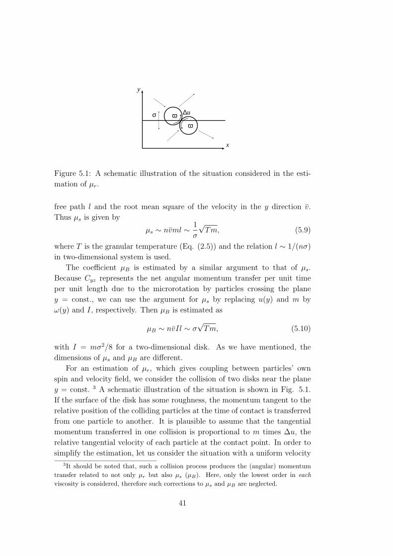
x

σ ωω

∆u

y

Figure 5.1: A schematic illustration of the situation considered in the esti-

mation of µr.

free path l and the root mean square of the velocity in the y direction v.

Thus µs is given by

µs ∼ nvml ∼ 1

σ

√Tm, (5.9)

where T is the granular temperature (Eq. (2.5)) and the relation l ∼ 1/(nσ)

in two-dimensional system is used.

The coefficient µB is estimated by a similar argument to that of µs.

Because Cyz represents the net angular momentum transfer per unit time

per unit length due to the microrotation by particles crossing the plane

y = const., we can use the argument for µs by replacing u(y) and m by

ω(y) and I, respectively. Then µB is estimated as

µB ∼ nvIl ∼ σ√

Tm, (5.10)

with I = mσ2/8 for a two-dimensional disk. As we have mentioned, the

dimensions of µs and µB are different.

For an estimation of µr, which gives coupling between particles’ own

spin and velocity field, we consider the collision of two disks near the plane

y = const. 3 A schematic illustration of the situation is shown in Fig. 5.1.

If the surface of the disk has some roughness, the momentum tangent to the

relative position of the colliding particles at the time of contact is transferred

from one particle to another. It is plausible to assume that the tangential

momentum transferred in one collision is proportional to m times ∆u, the

relative tangential velocity of each particle at the contact point. In order to

simplify the estimation, let us consider the situation with a uniform velocity

3It should be noted that, such a collision process produces the (angular) momentumtransfer related to not only µr but also µs (µB). Here, only the lowest order in eachviscosity is considered, therefore such corrections to µs and µB are neglected.

41

field, namely u′(y) = 0. 4 Then ∆u is given by ∆u ∼ 2(σ/2)ω(y). Be-

cause the frequency of collision per unit time per unit length near the plane

y = const. with the width σ is proportional to n2vσ2 in two-dimension, the

momentum transfer across the plane by collisions is estimated as

∆M ∼ n2vσ3m[2ω(y)]. (5.11)

Comparing Eq. (5.11) and the second term of Eq. (5.7) with u′(y) = 0, we

obtain

µr ∼ n2vσ3m ∼ n2σ3√

Tm. (5.12)

Summarizing the results above, which are consistent with Refs. [95–97],

we get following expressions for the coefficients of viscosity;

µB

µr

∼ 1

n2σ2∼ l2,

µs

µr

∼ 1

(nσ2)2∼

(l

σ

)2

. (5.13)

It should be noted that, because the dimension of µB is different from that

of µs and µr, we need to introduce another length scale to characterize the

macroscopic flow behavior in order to compare them. On the other hand, we

can see that, when the number density is high enough, µr becomes compara-

ble to µs, then the coupling between the angular momentum and the linear

momentum should play an important role.

5.3 Uniform Steady Solution of Flow on a

Slope

Now we present the uniform, steady solution of the micropolar fluid equations

(5.1), (5.2), and (5.3) on a slope, and compare the obtained profiles with the

result of numerical simulation.

Let us consider the two-dimensional steady flow on a slope under the

gravity. We take the x axis in the direction down the slope, and the y axis in

the direction perpendicular to the slope. The inclination angle of the slope

is θ, and the acceleration of gravity g = (g sin θ,−g cos θ, 0). In the uniform,

steady flow, mn = ρ = ρ(y), v = (u(y), 0, 0), and ω = (0, 0, ω(y)), therefore

4If we consider the situation with u′(y) 6= 0, we get ∆u = σ[u′(y) cos2 φ + ω(y)], whereφ is the angle between the y axis and the vector along the centerline from one particleto another. We need careful calculation in the average process of φ, which is beyondelementary kinetic theory.

42

the equation of continuity (5.1) is automatically satisfied. Eqs. (5.2) and

(5.3) reduce to following differential equations:

ρg sin θ +d

dy

[µs

du

dy+ µr

(du

dy+ 2ω

)]= 0, (5.14)

−ρg cos θ − dp

dy= 0, (5.15)

and

−2µr

(du

dy+ 2ω

)+

d

dy

[µB

dω

dy

]= 0. (5.16)

The equation of state for a two-dimensional granular gas has been derived in

Ref. [49], but here we adopt the lowest order estimate, namely, p = ρT/m, for

simplicity. We also assume the constant temperature T = T ; the validity is

of these assumptions is confirmed later in the comparison with the simulation

data. With the aid of these assumptions, we obtain the density profile from

Eq. (5.15);

ρ = ρ0 exp(−y

h

), h =

T

mg cos θ. (5.17)

Then, from the estimate of the coefficients Eq. (5.13), we introduce the

non-dimensional constants α0 and β0 as

µr

µs

= α0 exp(−2y/h),µB

µs

= β0σ2. (5.18)

After integrating Eqs. (5.14) and (5.16) with Eqs. (5.17) and (5.18), we

obtain the following relation between the velocity field u(y) and the micro-

rotation field ω(y);

u(Y ) = − exp(−Y )− β0ε2

2

dω(Y )

dY+ A0, (5.19)

where

u =u

ρ0gh2 sin θ/µs

, ω =ω

ρ0gh sin θ/µs

, (5.20)

with Y = y/h and ε = σ/h. Here, A0 is an integration constant. In the

integration of Eq. (5.14), we imposed the boundary condition for stress

tensor at the free surface, limy→∞ Syx → 0. From Eqs. (5.16) and (5.19), we

haved2ω(Y )

dY 2− 2

α0 exp(−2Y )

β0ε2

[exp(−Y ) + 2ω(Y )

1 + α0 exp(−2Y )

]= 0. (5.21)

43

Its general solution is given as the sum of a particular solution ωp and two

homogeneous solutions ω1 and ω2 by

ω(Y ) = Aω1(Y ) + Bω2(Y ) + ωp(Y ), (5.22)

with integration constants A and B. Changing the variable from Y to ν =

exp(−Y ), we can obtain the expressions

ωp =∞∑

k=1

a2k+1ν2k+1 with a3 =

2α0

9β0ε2, a2k+1 = f2k+1a2k−1,(5.23)

ω1 =∞∑

k=0

b2kν2k with b0 = 1, b2k = f2kb2k−2, (5.24)

and

ω2 = ω1 log ν +∞∑

k=1

c2kν2k

with c0 = 0, c2k = f2kc2k−2 − α0

k3

[1

β0ε2+ k − 1

]b2k−2, (5.25)

where

fk ≡ α0

k2

[4

β0ε2− (k − 2)2

]. (5.26)

Note that ωp and ω1 are regular but ω2 diverges at ν = 0 (Y →∞).

Now we show that the solution obtained from the micropolar fluid model

can quantitatively reproduce the results of numerical simulation. We use the

two dimensional DEM simulation data of collisional granular flow of identical

particles on a bumpy slope, which is presented in Chapter 6; the detail of the

simulation setup is given in that chapter. In the following, all quantities are

given in dimensionless form with the particle mass m, the particle diameter

σ, and the time unit τ =√

σ/g.

We used the data of the simulation with inclination sin θ = 0.45, system

size L = 1002, and number of flowing particle N = 1000. In the simulation,

uniform collisional flow is realized during 500 . t . 2000 where t is the

time as can be seen in Fig. 6.4. In order to determine the profiles of the

mean quantities describing the flow, we divide the space into layers which

are one particle diameter wide parallel to the slope, calculate the averages

inside layers, and then average the data over the time within the uniform

flow, 1000 ≤ t < 1500. The slope is made bumpy by attaching identical

44

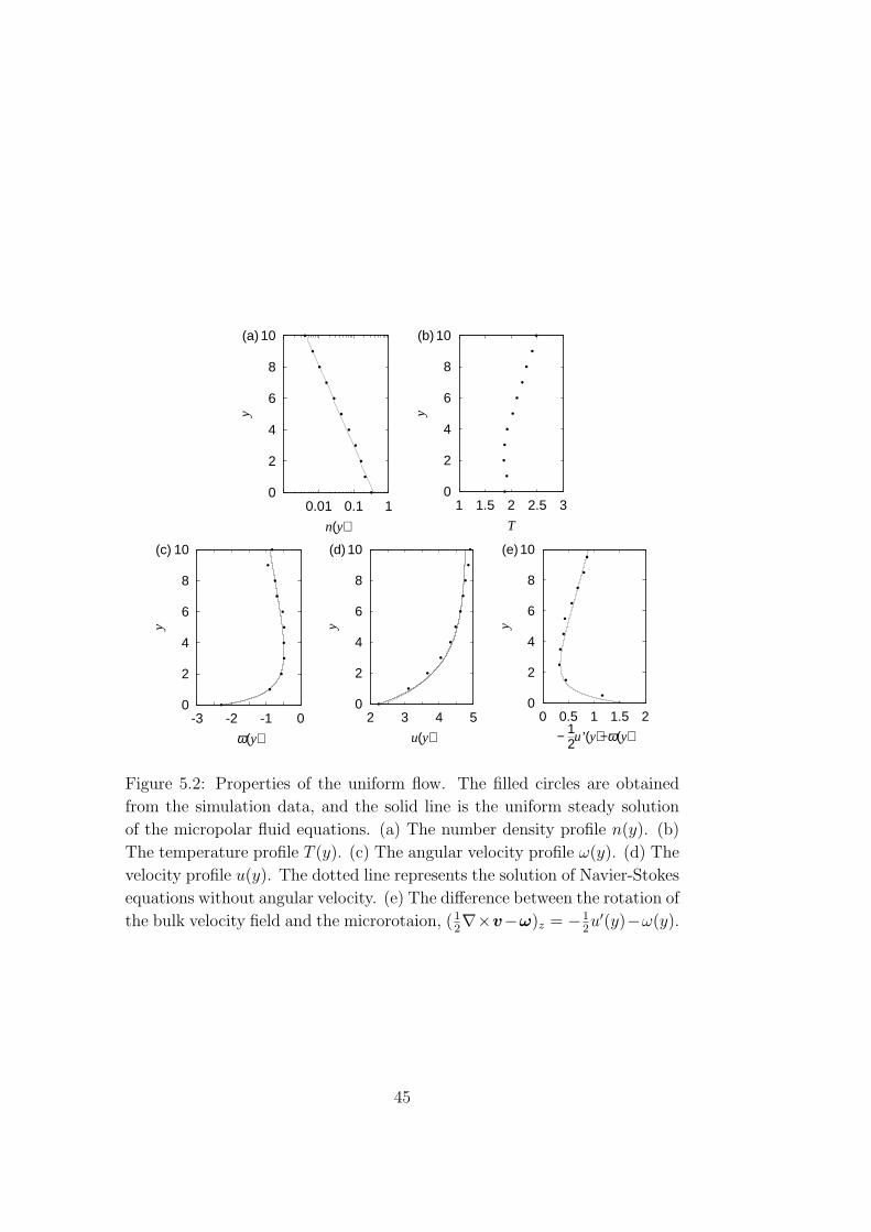
0

2

4

6

8

10

0.01 0.1 1

y

n(y)

(a)

0

2

4

6

8

10

1 1.5 2 2.5 3

y

T

(b)

0

2

4

6

8

10

-3 -2 -1 0

y

ω(y)

(c)

0

2

4

6

8

10

2 3 4 5

y

u(y)

(d)

0

2

4

6

8

10

0 0.5 1 1.5 2

y

− 12u’(y)−ω(y)

(e)

Figure 5.2: Properties of the uniform flow. The filled circles are obtained

from the simulation data, and the solid line is the uniform steady solution

of the micropolar fluid equations. (a) The number density profile n(y). (b)

The temperature profile T (y). (c) The angular velocity profile ω(y). (d) The

velocity profile u(y). The dotted line represents the solution of Navier-Stokes

equations without angular velocity. (e) The difference between the rotation of

the bulk velocity field and the microrotaion, (12∇×v−ω)z = −1

2u′(y)−ω(y).

45

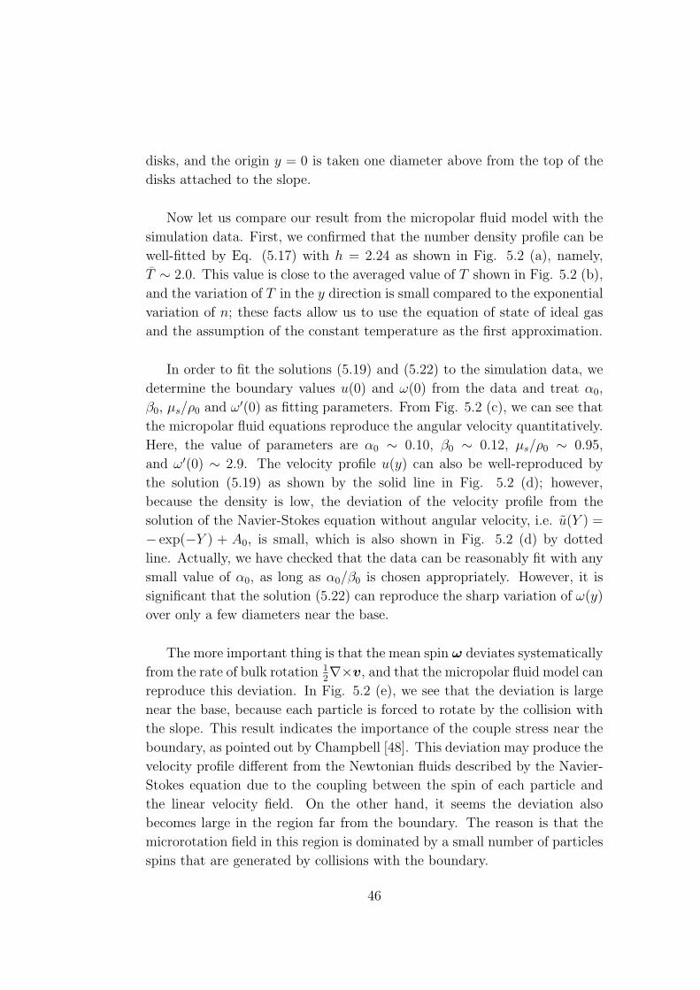
disks, and the origin y = 0 is taken one diameter above from the top of the

disks attached to the slope.

Now let us compare our result from the micropolar fluid model with the

simulation data. First, we confirmed that the number density profile can be

well-fitted by Eq. (5.17) with h = 2.24 as shown in Fig. 5.2 (a), namely,

T ∼ 2.0. This value is close to the averaged value of T shown in Fig. 5.2 (b),

and the variation of T in the y direction is small compared to the exponential

variation of n; these facts allow us to use the equation of state of ideal gas

and the assumption of the constant temperature as the first approximation.

In order to fit the solutions (5.19) and (5.22) to the simulation data, we

determine the boundary values u(0) and ω(0) from the data and treat α0,

β0, µs/ρ0 and ω′(0) as fitting parameters. From Fig. 5.2 (c), we can see that

the micropolar fluid equations reproduce the angular velocity quantitatively.

Here, the value of parameters are α0 ∼ 0.10, β0 ∼ 0.12, µs/ρ0 ∼ 0.95,

and ω′(0) ∼ 2.9. The velocity profile u(y) can also be well-reproduced by

the solution (5.19) as shown by the solid line in Fig. 5.2 (d); however,

because the density is low, the deviation of the velocity profile from the

solution of the Navier-Stokes equation without angular velocity, i.e. u(Y ) =

− exp(−Y ) + A0, is small, which is also shown in Fig. 5.2 (d) by dotted

line. Actually, we have checked that the data can be reasonably fit with any

small value of α0, as long as α0/β0 is chosen appropriately. However, it is

significant that the solution (5.22) can reproduce the sharp variation of ω(y)

over only a few diameters near the base.

The more important thing is that the mean spin ω deviates systematically

from the rate of bulk rotation 12∇×v, and that the micropolar fluid model can

reproduce this deviation. In Fig. 5.2 (e), we see that the deviation is large

near the base, because each particle is forced to rotate by the collision with

the slope. This result indicates the importance of the couple stress near the

boundary, as pointed out by Champbell [48]. This deviation may produce the

velocity profile different from the Newtonian fluids described by the Navier-

Stokes equation due to the coupling between the spin of each particle and

the linear velocity field. On the other hand, it seems the deviation also

becomes large in the region far from the boundary. The reason is that the

microrotation field in this region is dominated by a small number of particles

spins that are generated by collisions with the boundary.

46

5.4 Summary

In summary, the micropolar fluid model has been applied to a collisional

granular flow with relatively low density. It has been demonstrated that the

solution for uniform, steady flow on an inclined surface reproduces the results

of numerical simulation.

Because the density is low, the ideal gas assumption for the equation of

state and the estimation of the viscosity from the elementary kinetic theory

work well. In order to apply the model to denser collisional flows, we need a

systematic extension of the theory using, for example, Enskog theory. This

has already been done in the context of polyatomic fluids for completely

rough spheres without energy dissipation [96, 99] and it should be possible

to extend such results to the dissipative case [51]. The equation of state for

dense granular gas has also been discussed recently [8, 51].

On the other hand, the coupling between the particle spin and the velocity

field becomes stronger in dense frictional flows [100–102]. In some research,

the mechanics of granular media in dense quasi-static situation is considered

based on the micropolar or Cosserat theory [103, 104]. The concepts in mi-

cropolar mechanics may be helpful to understand the mechanics of granular

media, not only in the collisional flow regime but also in the denser situation.

47

Chapter 6

Steady State and its Instability

of Low-Density Collisional Flow

Most of researches on the collisional granular flow on a slope focus upon

the property of the steady uniform flow as referred in Chapter 2; in those

researches, the depth dependence of the flow properties such as velocity or

density profile is investigated, assuming that the flow is uniform in the di-

rection along the slope. It is known, however, that the granular materials

have the tendency to cluster due to the inelastic collision, which causes the

formation of density waves in the case of granular flow in a vertical pipe

[31, 32]. Therefore, it is natural to expect that this tendency will cause some

instability in the uniform flow on a slope.

Granular flow of an independent particle, or a single particle behavior,

has been studied as summarized in Section 2.1. It has been found to show

three types of motion depending on the inclination angle and roughness of the

slope; they are the static state (regime A), the steady motion with a constant

average velocity (regime B), and the accelerated motion (regime C). When we

increase the number of flowing particles, however, all the particles stop with

the inclination angle in regime B because the kinetic energy of the steady

motion is not large enough to overcome the energy loss through inelastic

collisions with other particles. It will give us an insight on the many-body

effect in the low-density granular flow to investigate how the single particle

picture is modified upon increasing the density of flowing particles.

In this chapter, we study how the single particle picture is modified in the

collisional flow with finite density by particle collisions. Based on numerical

simulations, we determine the parameter region where the uniform collisional

flow is realized with the finite density. Then we examine the stability of the

48

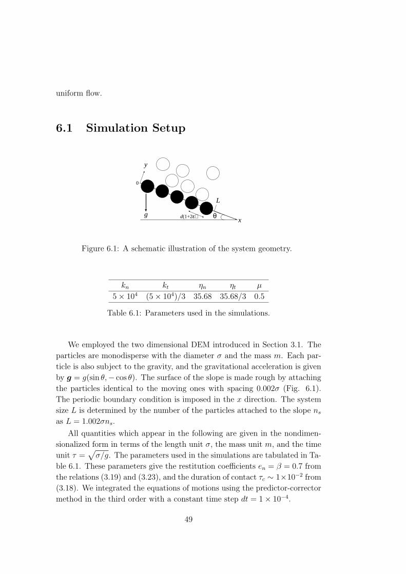
uniform flow.

6.1 Simulation Setup

x

y

θg d(1+2ε)

0

L

Figure 6.1: A schematic illustration of the system geometry.

kn kt ηn ηt µ

5× 104 (5× 104)/3 35.68 35.68/3 0.5

Table 6.1: Parameters used in the simulations.

We employed the two dimensional DEM introduced in Section 3.1. The

particles are monodisperse with the diameter σ and the mass m. Each par-

ticle is also subject to the gravity, and the gravitational acceleration is given

by g = g(sin θ,− cos θ). The surface of the slope is made rough by attaching

the particles identical to the moving ones with spacing 0.002σ (Fig. 6.1).

The periodic boundary condition is imposed in the x direction. The system

size L is determined by the number of the particles attached to the slope ns

as L = 1.002σns.

All quantities which appear in the following are given in the nondimen-

sionalized form in terms of the length unit σ, the mass unit m, and the time

unit τ =√

σ/g. The parameters used in the simulations are tabulated in Ta-

ble 6.1. These parameters give the restitution coefficients en = β = 0.7 from

the relations (3.19) and (3.23), and the duration of contact τc ∼ 1×10−2 from

(3.18). We integrated the equations of motions using the predictor-corrector

method in the third order with a constant time step dt = 1× 10−4.

49

6.2 Steady Flow from the Single Particle Limit

We first investigate how the uniform collisional flow appears when we increase

the density of flowing particles from the one particle limit.

As we have referred in Section 2.1, a single particle behavior depends on

the value of θ for a fixed roughness of the slope. It is known, however, that

the boundary between the regime B (the constant velocity regime) and C

(the acceleration regime) is not sharp; there is a parameter region where the

particle can attain steady state or can accelerate, depending on the initial

condition. We should also note that, when the initial kinetic energy of the

particle is too small, the particle may stop in the regime B and in part of the

regime C. In the present model with the parameters in Table 6.1, it turns

out that the regime A roughly corresponds to the region sin θ . 0.11, the

regime B to 0.11 . sin θ . 0.14, and the regime C to 0.16 . sin θ.

Now we focus on what happens when the number of moving particles

N is increased with the finite L. It is easy to expect that the dissipation

becomes larger upon increasing N , because the collisions between particles

or a particle and the slope become more frequent. Therefore it is obvious

that all the particles will stop irrespective of the initial condition if θ is in the

regime A. Even for any θ within the regime B, it turns out that the collisions

between particles eventually stop all the particles.

We examine closely the flowing behavior for the larger inclination angle θ

in the regime C. The situation is presented by showing the simulations with

sin θ = 0.45 and L = 20.04. We set the initial condition as follows:

xi(0) = (L/N)(i− 1), yi(0) = (1 + 2ε) + αξi, (6.1)

ui(0) = 0, vi(0) = 0, ωi(0) = 0, (6.2)

where xi(t) (yi(t)) and ui(t) (vi(t)) are the coordinate and the velocity of

center of mass of the ith particle at time t in the x (y) direction, respectively.

ωi(t) is the angular velocity of particle i at time t. ξi is a random number

uniformly distributed over the interval [0, 1]. The appropriate value of α is

a few times the diameter, and we adopted α = 3 ∼ 4 in actual simulations.

In the following, we define the ’density’ of the particles as ρ = N/L. In

the simulations with L = 20.04, we do not observe non-uniformity along

the slope in the particle distribution, therefore the parameter ρ is enough to

describe the situation. In order to characterize the qualitative difference of

accelerated behavior in the regime C and the uniform flow, we investigate

50

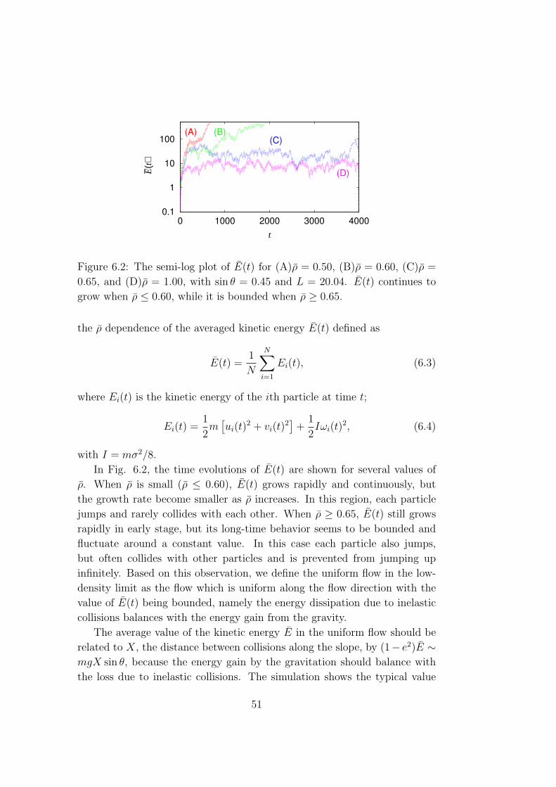
E– (t)

t

Figure 6.2: The semi-log plot of E(t) for (A)ρ = 0.50, (B)ρ = 0.60, (C)ρ =

0.65, and (D)ρ = 1.00, with sin θ = 0.45 and L = 20.04. E(t) continues to

grow when ρ ≤ 0.60, while it is bounded when ρ ≥ 0.65.

the ρ dependence of the averaged kinetic energy E(t) defined as

E(t) =1

N

N∑i=1

Ei(t), (6.3)

where Ei(t) is the kinetic energy of the ith particle at time t;

Ei(t) =1

2m

[ui(t)

2 + vi(t)2]+

1

2Iωi(t)

2, (6.4)

with I = mσ2/8.

In Fig. 6.2, the time evolutions of E(t) are shown for several values of

ρ. When ρ is small (ρ ≤ 0.60), E(t) grows rapidly and continuously, but

the growth rate become smaller as ρ increases. In this region, each particle

jumps and rarely collides with each other. When ρ ≥ 0.65, E(t) still grows

rapidly in early stage, but its long-time behavior seems to be bounded and

fluctuate around a constant value. In this case each particle also jumps,

but often collides with other particles and is prevented from jumping up

infinitely. Based on this observation, we define the uniform flow in the low-

density limit as the flow which is uniform along the flow direction with the

value of E(t) being bounded, namely the energy dissipation due to inelastic

collisions balances with the energy gain from the gravity.

The average value of the kinetic energy E in the uniform flow should be

related to X, the distance between collisions along the slope, by (1− e2)E ∼mgX sin θ, because the energy gain by the gravitation should balance with

the loss due to inelastic collisions. The simulation shows the typical value

51

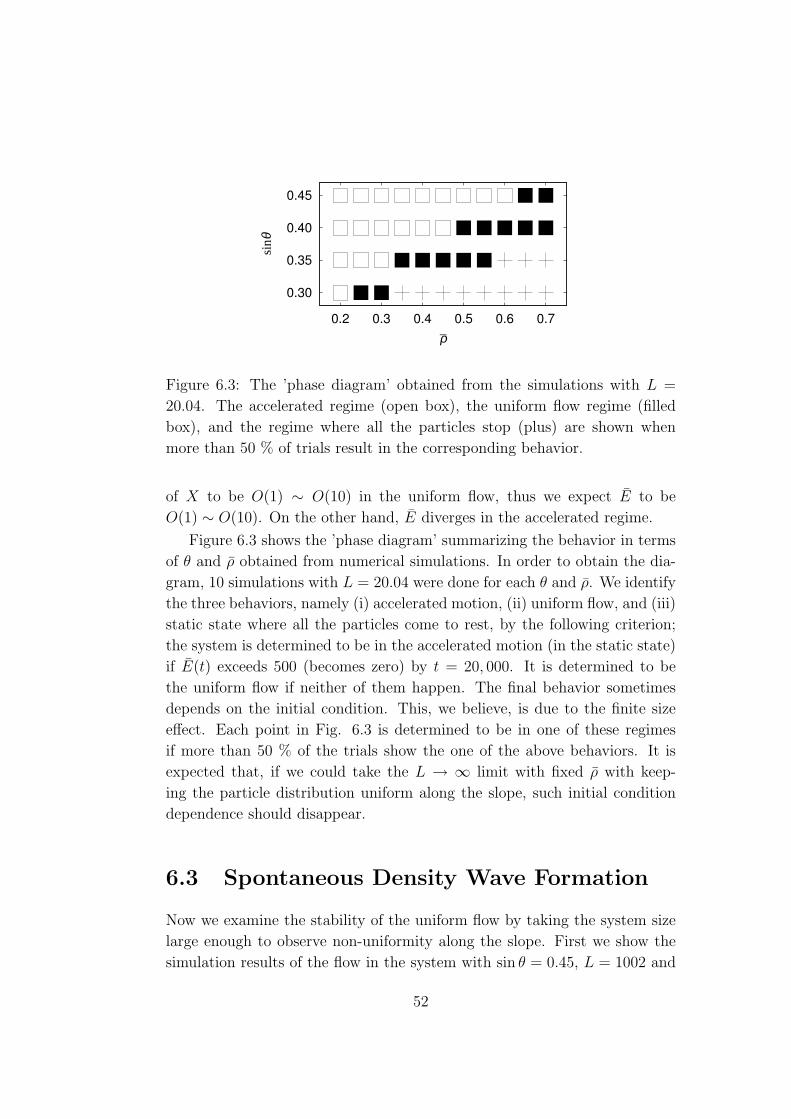
sinθ

ρ–

Figure 6.3: The ’phase diagram’ obtained from the simulations with L =

20.04. The accelerated regime (open box), the uniform flow regime (filled

box), and the regime where all the particles stop (plus) are shown when

more than 50 % of trials result in the corresponding behavior.

of X to be O(1) ∼ O(10) in the uniform flow, thus we expect E to be

O(1) ∼ O(10). On the other hand, E diverges in the accelerated regime.

Figure 6.3 shows the ’phase diagram’ summarizing the behavior in terms

of θ and ρ obtained from numerical simulations. In order to obtain the dia-

gram, 10 simulations with L = 20.04 were done for each θ and ρ. We identify

the three behaviors, namely (i) accelerated motion, (ii) uniform flow, and (iii)

static state where all the particles come to rest, by the following criterion;

the system is determined to be in the accelerated motion (in the static state)

if E(t) exceeds 500 (becomes zero) by t = 20, 000. It is determined to be

the uniform flow if neither of them happen. The final behavior sometimes

depends on the initial condition. This, we believe, is due to the finite size

effect. Each point in Fig. 6.3 is determined to be in one of these regimes

if more than 50 % of the trials show the one of the above behaviors. It is

expected that, if we could take the L → ∞ limit with fixed ρ with keep-

ing the particle distribution uniform along the slope, such initial condition

dependence should disappear.

6.3 Spontaneous Density Wave Formation

Now we examine the stability of the uniform flow by taking the system size

large enough to observe non-uniformity along the slope. First we show the

simulation results of the flow in the system with sin θ = 0.45, L = 1002 and

52

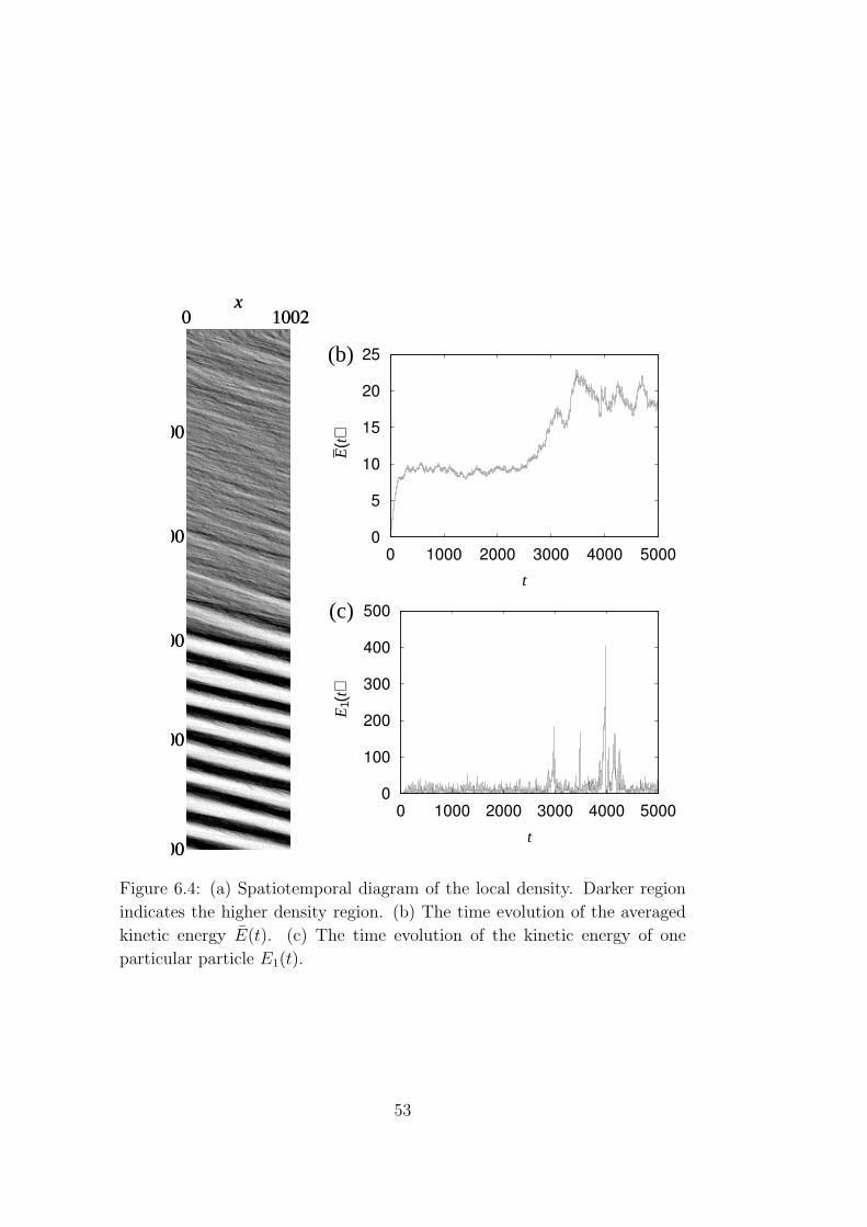
0 10020

1000

2000

3000

4000

5000

(a) x

t

(b)E– (t)

t

(c)

E1(

t)

t

Figure 6.4: (a) Spatiotemporal diagram of the local density. Darker region

indicates the higher density region. (b) The time evolution of the averaged

kinetic energy E(t). (c) The time evolution of the kinetic energy of one

particular particle E1(t).

53

N = 1000, i.e. ρ = 1.0. The initial condition is also given by Eq. (6.2),

therefore the particles are uniformly distributed along the slope at first.

Figure 6.4 (a) shows the spatiotemporal diagram of the local density along

the slope; the vertical axis is the time t, the horizontal axis is the coordinate

along the slope x, and the darker region represents the higher density region.

The y coordinates of the particles are not taken into account in that diagram.

In early stage, the density is almost uniform along the slope (300 . t .2000), namely uniform flow is realized. Then relatively large fluctuation

of density grows in the course of time (2000 . t . 3000); this means the

clustering behavior is triggered by the fluctuation. Finally system separate

into the high density region and the low density region, namely one large

cluster is formed (t & 3000). This cluster travels the system with almost

constant velocity because of the periodic boundary condition; we can see

that the cluster is stable once it is formed.

The time evolutions of the kinetic energy averaged over all particles, E(t),

and that of one particular particle, E1(t), are also shown in Figs. 6.4 (b) and

(c), respectively. Both of them are almost constant in the stage of uniform

flow. Then E(t) increases in 2000 . t . 3000. In t & 3000, the fluctuation

of E1(t) becomes considerably large, and E(t) begins to fluctuate around

another constant value which is larger than the one in the stage of uniform

flow. The reason why the kinetic energy increases when a cluster is formed

can be understood as follows: When the cluster is formed, the region with the

density lower than the threshold value to maintain the steady flow (∼ 0.65

in the case of sin θ = 0.45, see Fig. 6.3.) appears locally, and particles in

such a spatial region can be highly accelerated. However, the particle will

be caught in the cluster sooner or later, and then quickly lose its kinetic

energy. This mechanism maintains the moving cluster, and results in the

large fluctuations in E1(t).

The situations are clearer in Figs. 6.5, which show the snapshots of the

particle configuration and the local density (number of particles per unit

length) at (a) t = 0 (initial condition), (b) t = 1500 (uniform flow stage),

and (c) t = 5000 (clustering stage). The red circles in the figures express the

particles, but the diameters are ten times larger than the real scale for better

sight. The initial condition is completely uniform along the slope as shown

in Fig. 6.5 (a). In the uniform flow stage, Fig. 6.5 (b), the uniform particle

distribution is realized with some fluctuation. Figure 6.5 (c) of the clustering

stage shows that the particles in the low density region are jumping up, while

those in the dense region stay close to the floor.

54

(a)

0123

dens

ity

(b)

0123

dens

ity

(c)

0123

0 100 200 300 400 500 600 700 800 900 1000

dens

ity

x

Figure 6.5: The snapshots of the particle configuration (upper figures) and

the local density (lower figures) at t = 0 (a), t = 1500 (b), t = 5000 (c).

The red circles in the upper figures express the flowing particles, but the

diameters of circles are ten times larger than the real scale for better sight.

We also find that the instability depends on the system size L and the

“density” ρ. In Figs. 6.6, spatiotemporal diagrams of the local density with

the different values of L and ρ are shown. From the comparison of Fig. 6.4

(a), Figs. 6.6 (a) and (b), which are the simulation results with ρ = 1.0

but different L, we can see that the instability becomes weaker for smaller

system sizes. From Fig. 6.6 (a), (c), and (d), which are the results with

L = 501 but different ρ, we find that the higher the density is, the more

stable the uniform flow is. It can also be seen that, even though the clear

cluster formation has not been found in Fig. 6.6 (a), the density fluctuation

is quite large. We have also simulated the system with the same L and N

as in Fig. 6.6 (a) but with the initial configuration with large inhomogeneity

along the flow direction (Fig. 6.6 (e)). It is found that, a cluster is formed

after a while, but it almost disappears when the head and the tail of the

cluster collide through the periodic boundary condition (3000 ≤ t ≤ 4000).

55

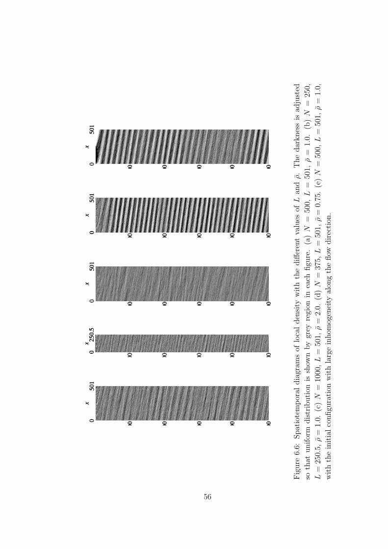
050

10

1000

2000

3000

4000

5000

(a)

x

t

025

0.5

0

1000

2000

3000

4000

5000

(b)

x

t

050

10

1000

2000

3000

4000

5000

(c)

x

t

050

10

1000

2000

3000

4000

5000

(d)

x

t

050

10

1000

2000

3000

4000

5000

(e)

x

t

Fig

ure

6.6:

Spat

iote

mpor

aldia

gram

sof

loca

lden

sity

wit

hth

ediff

eren

tva

lues

ofL

and

ρ.

The

dar

knes

sis

adju

sted

soth

atunifor

mdis

trib

uti

onis

show

nby

grey

regi

onin

each

figu

re.

(a)

N=

500,

L=

501,

ρ=

1.0.

(b)

N=

250,

L=

250.

5,ρ

=1.

0.(c

)N

=10

00,L

=50

1,ρ

=2.

0.(d

)N

=37

5,L

=50

1,ρ

=0.

75.

(e)

N=

500,

L=

501,

ρ=

1.0,

wit

hth

ein

itia

lco

nfigu

rati

onw

ith

larg

ein

hom

ogen

eity

alon

gth

eflow

dir

ecti

on.

56

6.4 Summary

We have examined the two-dimensional granular flow on a rough slope in

the collisional flow regime by numerical simulations. It was shown that the

mutual collisions among particles stabilizes the flow even in the accelerated

regime for a single particle system. The phase diagram was determined for

the accelerated, uniform flow, and stopping regime in terms of the particle

density ρ and the inclination angle θ for a particular system size. The stability

of uniform flow was also examined and we found that a large single cluster

appears spontaneously out of a uniform initial state. It was shown that the

smaller the particle density is, or the larger the system size is, the less stable

the uniform flow is.

In the case where the uniform flow was unstable (Figs. 6.4(a) and 6.6(d)),

the fluctuation grew up to form a large cluster. The final state was that one

stable cluster travels the system with almost constant velocity; it was due to

the finite size effect under the periodic boundary condition. The reason why

the formed cluster was almost broken in the case of L = 501 and ρ = 1.0

(Fig. 6.6(e)) was that the head and the tail of the cluster interacted through

the periodic boundary condition, namely, it was also the finite size effect.

Based on these observations, we guess that, if we perform a simulation

or an experiment of initially uniform flow in a very long system under an

open boundary condition, the small clusters merge to form larger clusters as

they go downstream. It is a future issue to investigate the instability in more

realistic situations 1.

The spontaneous cluster formation out of uniform flow is seen also in

the granular flow through a vertical pipe [31, 32] and in the traffic flow on a

freeway [105–107]. It is an interesting problem to find out whether those phe-

nomena and the cluster formation found here have a common mathematical

structure at phenomenological level.

1In the wave formation observed in a recent experiment of shallow granular flow on aslope [61], it has been found that the wavelength becomes longer in the downstream.

57

Chapter 7

Concluding Remarks

In this thesis, we investigated the fundamental properties of the gravitational

granular flow. We chose the flow on a slope as a model system because, in

spite of its simple setup, all types of granular flows are realized by changing

the inclination angle, the roughness of the slope, or the density of particles.

It is a system suitable for the comprehensive research on granular flow.

We examined the particle stiffness dependence of the steady flows numer-

ically by taking the inelastic hard sphere limit of the soft sphere model. In

the case of the collisional flow, the collision rate is almost constant and the

contact time fraction approaches to zero, which means the interaction be-

tween particles converges to the binary collisions in the inelastic hard sphere

model. On the other hand, the collision rate diverges in the power law of

the stiffness parameter in the frictional flow. The estimated time fraction

for the multiple or the sustained contact remains finite even in the hardest

case. This suggests that the interaction in the frictional flow can never be

expressed by the binary collisions: even in the hard sphere limit, particles

experience the lasting multiple contact.

The inelastic hard sphere picture of the granular material in the colli-

sional flow regime allows us to use the kinetic theory and the hydrodynamic

model. We applied the micropolar fluid model to the collisional granular

flow in which the effect of the spinning motion of particles is incorporated.

The adopted constitutive equations were the straightforward extension of the

Navier-Stokes equation. We used the simple estimate of the viscosities based

on the elementary kinetic theory, and obtained the analytical solution of the

steady flow on a slope. It was demonstrated that the solution reproduces

quantitatively the deviation of the particle spin from the vorticity of the

mean velocity field in the numerical simulation.

58

It was shown by the numerical simulation that the uniform collisional

flow exhibits the dynamical instability. We determined the parameter region

where the collisional uniform flow is realized with the finite density for a

particular system size. Then we performed the simulation in the very long

system, and it was found that the uniform flow shows the clustering insta-

bility. It was demonstrated that the uniform flow is less stable for the longer

system size and/or the lower density.

These results are informative for linking the understandings of the low-

density rapid flow to the dense slow flow. The qualitative difference of the

stiffness dependence between the collisional flow and the frictional flow is

helpful to quantify the dominant interaction in the situation where both the

inelastic collision and the sustained contact occurs. The coupling between

the spinning motion of particles and the mean velocity becomes stronger

for the denser flow. The clustering instability results in coexistence of dense

regions and dilute regions. We hope that the future extension of our research

will help to understand the nature of transition between the collisional flow

and the frictional flow, and finally to construct the comprehensive theory of

granular flow.

59

Acknowledgement

I would like to express my sincere gratitude to my adviser, Prof. Hiizu

Nakanishi, for his patient and continuous encouragement, valuable stimu-

lating discussions, and critical comments on the present thesis and all of

my studies. His dedicated guidance has been instrumental in my academic

development. I am also grateful to Prof. Hisao Hayakawa for his encourage-

ment, helpful suggestions, and collaborations. I learned a lot about granular

physics through fruitful discussions with him. The encouragement, valuable

discussions and comments on the present thesis by Prof. Hiroshi Kawai and

Prof. Masayuki Tokita are also acknowledged very much.

Thanks are also due to Prof. Kiyohide Nomura and Dr. Yumino Hayase

for their helpful comments on my studies and computation. I am very thank-

ful to Prof. Takashi Odagaki, Prof. Akira Yoshimori, and Dr. Jun Matsui

for valuable comments on the thesis work and advice on my studies. I would

like to thank Mr. Masashi Torikai, Dr. Masaharu Isobe, and all members of

statistical physics and condensed matter theory research groups at Kyushu

University for valuable discussions and friendships.

I would like to acknowledge the warm hospitality of people in Kyoto

during my stay at Yukawa Institute for Theoretical Physics in winter, 2001,

where part of my thesis work has been carried out.

Part of the computation in this work has been done using the facilities

of the Supercomputer Center, Institute for Solid State Physics, University of

Tokyo. This research is partially supported by Hosokawa powder technology

foundation and Grant-in-Aid for JSPS Research Fellows.

Finally I gratefully thank my family and friends for their warm supports

and encouragement.

60

Appendix A

Derivation of the Micropolar

Fluid Equations

We outline the derivation of the micropolar fluid equations (5.1) - (5.3) from

the conservation laws of mass, momentum, and angular momentum. The

derivation here is based on Ref. [29].

A.1 Equation of Continuity

We consider a volume V (t) which moves with the fluid and whose surface is

Ω(t).

From the conservation law of mass, we obtain

d

dt

∫

V (t)

ρdr = 0. (A.1)

Using the relation

d

dt

∫

V (t)

G(r, t)dr =

∫

V (t)

[∂tG + v · ∇G + G∇ · v]dr (A.2)

for an arbitrary scalar function G(r, t) [108], we get the equation of continu-

ity;

∂tρ +∇ · ρv = 0 ⇔ Dρ

Dt+ ρ∇ · v = 0. (A.3)

61

A.2 Equation of Motion

The conservation of momentum is written as

d

dt

∫

V (t)

ρvdr =

∫

V (t)

ρfdr +

∫

Ω(t)

S · ndΩ, (A.4)

where f is the force per unit mass and S is the stress tensor 1. Using Gauss’

theorem, we obtain

ρD

Dtv = ρf +∇ · S. (A.5)

Here we used the equation of continuity (A.3) and the relation (A.2).

A.3 Equation of Microrotation

From Eqs. (A.2) and (A.5), we have

d

dt

∫

V (t)

ρ(r × v)dr (A.6)

=

∫

V (t)

[∂t(r × ρv) + (v · ∇)(r × ρv) + (r × ρv)(∇ · v)]dr (A.7)

=

∫

V (t)

r × [ρDtv]dr (A.8)

=

∫

V (t)

r × [ρf +∇ · S]dr. (A.9)

On the other hand, the conservation of the angular momentum is ex-

pressed as

d

dt

∫

V (t)

ρ[l+r×v]dr =

∫

V (t)

ρ[r×f ]dr+

∫

Ω(t)

[C ·n+r×(S ·n)]dΩ (A.10)

with the angular momentum of the microrotaion ρl 2 and the couple stress

C. 3

1The component of the stress tenser Sij is defined as the j component of the forceacting on the plane perpendicular to the i direction. Therefore, the inner product of thetensor and the vector S · n means Sjinj and (∇ · S)i ≡ ∂jSji.

2ρl ≡ nIω in the system consists of identical spheres whose moments of inertia are I.Here, n and ω are the number density and the angular velocity field, respectively.

3Here we do not consider the external torque, because such a term do not appear inthe granular media.

62

When we use∫

V (t)

[r × (∇ · S)]idr (A.11)

=

∫

V (t)

[εijkrj∂mSmk]dr (A.12)

=

∫

V (t)

[εijk(∂mrjSmk − Sjk)]dr (A.13)

=

∫

V (t)

[∂m(εijkrjSmk)dr −∫

V (t)

(εijkSjk)dr (A.14)

=

∫

Ω(t)

[r × S · n]dΩ−∫

V (t)

(εijkSjk)dr, (A.15)

we get ∫

Ω(t)

[r × S · n]dΩ =

∫

V (t)

[r × (∇ · S) + s(a)]dr (A.16)

by using the vector defined from the asymmetric part of the stress tensor,

s(a)i ≡ εijkSjk. Thus Eq. (A.10) reads

d

dt

∫

V (t)

ρ[l + r×v]dr =

∫

V (t)

[ρr×f +∇·C + r× (∇·S)+ s(a)]dr. (A.17)

Considering Eq. (A.9), we obtain

d

dt

∫

V (t)

ρldr =

∫

V (t)

[∇ · C + s(a)]dr. (A.18)

Again from Eqs. (A.2) and (A.3), we have

d

dt

∫

V (t)

ρldr =

∫

V (t)

[∂tρl + v · ∇ρl + ρl∇ · v]dr (A.19)

=

∫

V (t)

ρ[∂t + v · ∇]ldr. (A.20)

From Eqs. (A.18) and (A.20), we finally obtain

ρD

Dtl = ∇ · C + s(a). (A.21)

63

Appendix B

A Soft Ball on the Floor

When a soft ball is in contact with the floor, the equation of motion for the

overlap of the ball and the floor, z, is given by Eq. (4.4);

z + knz + ηnz = g. (B.1)

The solution of this equation is

z(t) = exp

(−1

2ηnt

)[− g

kn

cos(Ωt) + B(v0) sin(Ωt)

]+

g

kn

, (B.2)

where

Ω =

√kn − η2

n

4, (B.3)

and

B(v0) =v0 − gηn/(2kn)

Ω. (B.4)

Here we have assumed that the impact velocity is v0. Note that ηn ∝√

kn

(see Eq. (4.1)) and thus Ω ∝ √kn. The collision ends when z(Tc) = 0, and

the restitution coefficient is determined by |z(Tc)/v0|.When v0 ∼ O(1) >> 1/

√kn, the solution (B.2) is approximated as

z(t) = exp

(−1

2ηnt

) [v0

Ωsin(Ωt)

]+ O

(k−1

n

). (B.5)

The leading order gives the constant restitution coefficient ew = exp(−ηnτw/2)

with the constant duration of contact with the floor τw = π/Ω.

The critical impact velocity vc below which the the ball stays in contact

with the floor is determined by the condition z(Tc) = 0, where Tc is the

smallest positive solution of z(Tc) = 0. The constant ew based on Eq. (B.5)

64

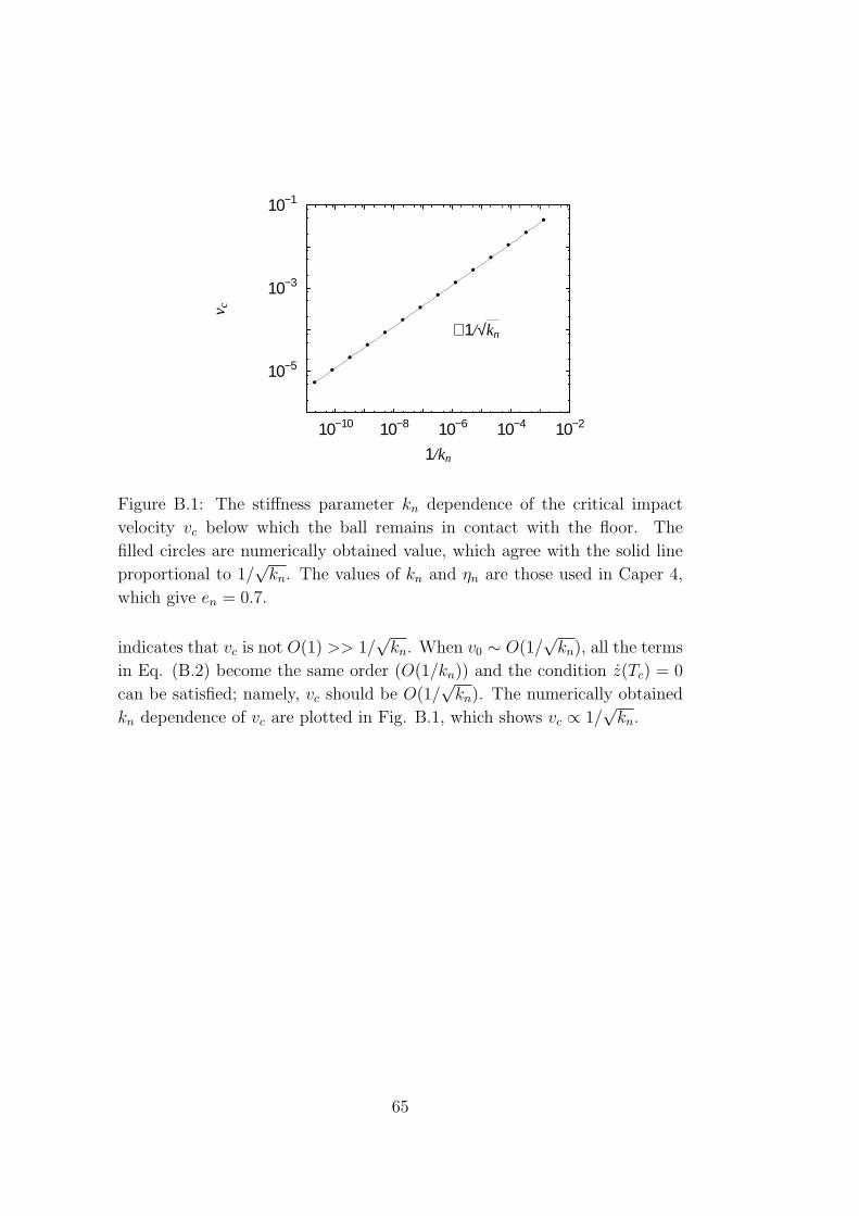
10−5

10−3

10−1

10−10 10−8 10−6 10−4 10−2

v c

1/kn

∝1/√kn

Figure B.1: The stiffness parameter kn dependence of the critical impact

velocity vc below which the ball remains in contact with the floor. The

filled circles are numerically obtained value, which agree with the solid line

proportional to 1/√

kn. The values of kn and ηn are those used in Caper 4,

which give en = 0.7.

indicates that vc is not O(1) >> 1/√

kn. When v0 ∼ O(1/√

kn), all the terms

in Eq. (B.2) become the same order (O(1/kn)) and the condition z(Tc) = 0

can be satisfied; namely, vc should be O(1/√

kn). The numerically obtained

kn dependence of vc are plotted in Fig. B.1, which shows vc ∝ 1/√

kn.

65

Bibliography

[1] H. M. Jaeger, S. R. Nagel, and R. P. Behringer. Granular solids, liquids,

and gases. Rev. Mod. Phys., Vol. 68, No. 4, p. 1259, October 1996.

[2] L. P. Kadanoff. Built upon sand: Theoretical ideas inspired by granular

flows. Rev. Mod. Phys., Vol. 71, No. 1, p. 435, 1999.

[3] P. G. de Gennes. Granular matter: a tentative view. Rev. Mod. Phys.,

Vol. 71, p. S374, 1999.

[4] Ancey C. Dry granular flows down an inclined channel: Experimental

investigations on the frictional-collisional regime. Phys. Rev. E, Vol. 65,

p. 011304, 2001.

[5] P. K. Haff. Grain flow as a fluid-mechanical phenomenon. J. Fluid

Mech., Vol. 134, p. 401, 1983.

[6] J. T. Jenkins and S. B. Savage. A theory for the rapid flow of identical,

smooth, nearly elastic, spherical particles. J. Fluid Mech., Vol. 130, p.

187, 1983.

[7] C. S. Campbell. Rapid granular flows. Ann. Rev. Fluid Mech., Vol. 22,

p. 57, 1990.

[8] T. Poschel and S. Luding, editors. Granular Gases. Springer-Verlag,

Berlin, Germany, 2001.

[9] N. Sela and I. Goldhirsch. Hydrodynamic equations for rapid flows of

smooth inelastic spheres, to Burnett order. J. Fluid Mech., Vol. 361,

p. 41, 1998.

[10] I. Goldhirsch. in Modeling in Applied Sciences: A Kinetic Theory

Approach. Birkhauser, Boston, 2000.

66

[11] J. Duran. Sands, Powders, and grains: introduction to the physics of

granular materials. Springer, New York, 1997.

[12] M. Isobe. Simple and efficient algorithm for large scale molecular dy-

namics simulation in hard disk systems. Int. J. Mod. Phys., Vol. C10,

p. 1281, 1999.

[13] P. A. Cundall and O. D. L. Strack. A discrete numerical model for

granular assemblies. Geotechnique, Vol. 29, p. 47, 1979.

[14] T. Poschel. Granular material flowing down an inclined chute: a molec-

ular dynamics simulation. J. Phys. II (France), Vol. 3, p. 27, 1993.

[15] X. M. Zheng and J. M. Hill. Molecular dynamics simulation of granular

flows: Slip along rough inclined planes. Comput. Mech., 1998.

[16] D. Ertas, G. S. Grest, T. C. Halsey, D. Levine, and L. E. Silbert.

Gravity-driven dense granular flows. Europhys. Lett., Vol. 56, p. 214,

2001.

[17] L. E. Silbert, D. Ertas, G. S. Grest, T. C. Halsey, D. Levine, and S. J.

Plimpton. Granular flow down an incline plane: Bagnold scaling and

rheology. Phys. Rev. E, Vol. 64, p. 051302, 2001.

[18] L. E. Silbert, G. S. Grest, S. J. Plimpton, and D. Levine. Bound-

ary effects and self-organization in dense granular flows. Phys. Fluids,

Vol. 14, p. 2637, 2002.

[19] L. E. Silbert, D. Ertas, G. S. Grest, T. C. Halsey, and D. Levine. Analo-

gies between granular jamming and the liquid-gas transition. Phys.

Rev. E, Vol. 65, p. 051307, 2002.

[20] S. Yuu, T. Abe, T. Saitoh, and T. Umekage. Three-dimensional numer-

ical simulation of the motion of particles discharging from a rectangular

hopper using distinct element method and comparison with experimen-

tal data (effects of time steps and material properties. Advanced Powder

Technol., Vol. 6, p. 259, 1995.

[21] Y. Taguchi. Funryutai no Dourikigaku [in Japanese]. In H. Nishimori,

H. Hayakawa, and Y. Taguchi, editors, Physics of Granular Matter,

Vol. XI of Selected Papers in Physics, p. 30. The Physical Society of

Japan, 1999.

67

[22] S. R. Kim and L. V. Woodcock. Kinetic theory of granular shear flow:

constitutive relations for the hard sphere model. J. Stat. Phys., Vol. 71,

p. 174, 1993.

[23] H. Xu, M. Y. Louge, and J. T. Jenkins. Flow development of a sheared

collisional granular flow. In Y. Kishino, editor, Powders and Grains

2001, p. 359, 2001.

[24] T. G. Drake. Granular flow: physical experiments and their impli-

cations for microstructual theories. J. Fluid Mech., Vol. 225, p. 121,

1991.

[25] J. Cao, G. Ahmai, and M. Massoudi. Gravity granular flows of slightly

frictional particles down an inclined bumpy chute. J. Fluid Mech., Vol.

316, p. 197, 1996.

[26] E. Azanza, R. Chevoir, and P. Moucheront. Experimental study of

collisional granular flows down an inclined plane. J. Fluid Mech., Vol.

400, p. 199, 1999.

[27] A. C. Eringen. Simple microfluids. Int. J. Engng. Sci., Vol. 2, p. 205,

1964.

[28] A. C. Eringen. Theory of micropolar fluids. J. Math. Mech., Vol. 16,

p. 1, 1966.

[29] G. Lukazewicz. Micropolar Fluids: Theory and Applications.

Birkhauser, Boston, 1999.

[30] H. Hayakawa. Slow viscous flows in micropolar fluids. Phys. Rev. E,

Vol. 61, p. 5477, 2000.

[31] S. Horikawa, A. Nakahara, T. Nakayama, and M. Matsushita. Self-

organized critical density waves of granular material flowing through a

pipe. J. Phys. Soc. Jpn., Vol. 64, p. 1870, 1995.

[32] M. Y. Louge. Computer simulations of rapid granular flows of spheres

interacting with a flat, frictional boundary. Phys. Fluids, Vol. 6, p.

2253, 1994.

[33] F.-X. Riguidel, R. Jullien, G. H. Ristow, A. Hansen, and D. Bideau.

Behavior of a sphere on a rough inclined plane. J. Phys. I (France),

Vol. 4, p. 261, 1994.

68

[34] G. H. Ristow, F. X. Ringuidel, and D. Bideau. Different characteristics

of the motion of a single particle on a bumpy inclined plane. J. Phys.

I (France), Vol. 4, p. 1161, 1994.

[35] F. X. Ringuidel, A. Hansen, and D. Bideau. Gravity-driven motion of

a particle on an inclined plane with controlled roughness. Europhys.

Lett., Vol. 28, p. 13, 1994.

[36] S. Dippel, G. G. Batrouni, and D. E. Wolf. Collision-induced friction

in the motion of a single particle on a bumpy inclined line. Phys. Rev.

E, Vol. 54, p. 6845, 1996.

[37] L. Samson, I. Ippolito, G. G. Batrouni, and J. Lemaitre. Diffusive

properties of motion on a bumpy plane. Euro. Phys. J. B, Vol. 3, p.

377, 1998.

[38] L. Quartier, B. Andreotti, S. Douady, and A. Daerr. Dynamics of a

grain on a sandpile model. Phys. Rev. E, Vol. 62, p. 8299, 2000.

[39] G. G. Batrouni, S. Dippel, and L. Samson. Stochastic model for the

motion of a particle on an inclined plane and the onset of viscous

friction. Phys. Rev. E, Vol. 53, p. 6469, 1996.

[40] S. Dippel, G. G. Batrouni, and D. E. Wolf. How transversal fluctuations

affect the friction of a particle on a rough incline. Phys. Rev. E, Vol. 56,

p. 3645, 1997.

[41] R. A. Bagnold. Experiments on a gravity-free dispersion of large solid

spheres in a newtonian fluid under shear. Proc. Roy. Soc. Lond. A,

Vol. 225, p. 49, 1954.

[42] S. Chapman and T. G. Cowling. The mathematical theory of non-

uniform gases. Cambridge university press, Cambridge, 1970.

[43] I. Goldhirsch and G. Zanetti. Clustering instability in dissipative gases.

Phys. Rev. Lett., Vol. 70, p. 1619, 1993.

[44] S. McNamara and W. R. Young. Dynamics of a freely evolving, two-

dimensional granular medium. Phys. Rev. E, Vol. 53, p. 5089, 1996.

[45] T. P. C. van Noije and M. H. Ernst. Cahn-hilliard theory for unstable

granular fluids. Phys. Rev. E, Vol. 61, p. 1745, 2000.

69

[46] H. Nakanishi. Velocity distribution of inelastic granular gas in homo-

geneous cooling state. cond-mat/0208477, 2002.

[47] J. Bougie, S. J. Moon, J. B. Swift, and H. L. Swinney. Shocks in

vertically oscillated granular layers. Phys. Rev. E, Vol. 66, p. 051301,

2002.

[48] C. S. Champbell. Boundary interactions for two-dimensional granular

flows. part 1. flat boundaries, asymmetric stresses and couple stresses.

J. Fluid Mech., Vol. 247, p. 111, 1993.

[49] J. T. Jenkins and M. W. Richman. Kinetic theory for plane flows of

a dense gas of identical, rough, inelastic, circular disks. Phys. Fluids,

Vol. 28, p. 3485, 1985.

[50] C. K. K. Lun and S. B. Savage. A simple kinetic-theory for granular

flow of rough, inelastic, spherical-particles. J. Appl. Mech., Vol. 54,

p. 47, 1987.

[51] C. K. K. Lun. Kinetic theory for granular flow of dense, slightly inelas-

tic, slightly rough spheres. J. Fluid Mech., Vol. 233, p. 539, 1991.

[52] K. Kanatani. Funryutai no ryudo no kiso riron [in japanese]. Trans.

Jpn. Soc. Mech. Eng. B, Vol. 45, pp. 507,515, 1979.

[53] J. Kano, A. Shimosaka, , and J. Hidaka. ryudo ryushigun no kousei

kankei ni kansuru ichi kousatsu [in Japanese]. J. Soc. Powder Technol.

Jpn., Vol. 33, p. 95, 1996.

[54] T. G. Drake. Structual features in granular flows. J. Geophys. Res.,

Vol. 95, p. 8681, 1990.

[55] M. A. Hopkins and M. Y. Louge. Inelastic microstructure in rapid

granular flows of smooth disks. Phys. Fluids A, Vol. 3, p. 47, 1991.

[56] O. Moriyama, N. Kuroiwa, M. Matsushita, and H. Hayakawa. 4/3 law

of granular particles flowing through a vertical pipe. Phys. Rev. E,

Vol. 80, p. 2833, 1998.

[57] J.-L. Aider, N. Sommier, T. Raafat, and J.-P. Hulin:. Experimental

study of a granular flow in a vertical pipe: A spatiotemporal analysis.

Phys. Rev. E, Vol. 59, p. 778, 1999.

70

[58] J. Lee and M. Leibig. Density waves in granular flow: a kinetic wave

approach. J. Phys. I France, Vol. 4, p. 507, 1994.

[59] J. Lee. Density waves in the flows of granular media. Phys. Rev. E,

Vol. 49, p. 281, 1994.

[60] T. Poschel. Recurrent clogging and density waves in granular material

flowing through a narrow pipe. J. Phys. I France, Vol. 4, p. 499, 1994.

[61] S. N. Prasad, D. Pal, and M. J. M. Romkens. Wave formation on a

shallow layer of flowing grains. J. Fluid Mech., Vol. 413, p. 89, 2000.

[62] M. Y. Louge and S. C. Keast. On dense granular flows down flat

frictional inclines. Phys. Fluids, Vol. 13, p. 1213, 2001.

[63] T. S. Komatsu, S. Inagaki, N. Nakagawa, and S. Nasuno. Creep motion

in granular pile exhibiting steady surface flow. Phys. Rev. Lett., Vol. 86,

p. 1757, 2001.

[64] A. V. Orpe and D. V. Khakhar. Scaling relations for granular flow

in quasi-two-dimensional rotating cylinders. Phys. Rev. E, Vol. 64, p.

031302, 2001.

[65] D. Bonamy, F. Daviaud, L. Laurent, M. Bonetti, and J. P. Bouchaud.

Multiscale clustering in granular surface flows. Phys. Rev. Lett., Vol. 89,

p. 034301, 2002.

[66] S. B. Savage. Gravity flow of cohesionless granular materials in chutes

and channels. J. Fluid Mech., Vol. 92, p. 53, 1979.

[67] L. E. Silbert, J. W. Landry, and G. S. Grest. Granular flow down a

rough inclined plane: transition between thin and thick piles. cond-

mat/0206188, 2002.

[68] P. C. Johnson and R. Jackson. Frictional-collisional constitutive re-

lations for granular materials, with application to plane shearing. J.

Fluid Mech., Vol. 176, p. 67, 1987.

[69] P. Mills, D. Loggia, and M. Tixier. Model for a stationary dense gran-

ular flow along an inclined wall. Europhys. Lett., Vol. 45, p. 733, 1999.

[70] B. Andreotti and S. Douady. Selection of velocity profile and flow depth

in granular flows. Phys. Rev. Lett., Vol. 63, p. 0131305, 2001.

71

[71] S. Douady, B. Andreotti, and A. Daerr. On granular surface flow equa-

tions. Eur. Phys. J. B, Vol. 11, p. 131, 1999.

[72] A. Aradian, E. Raphael, and P.-G. de Gennes. Surface flows of granular

materials: A short introduction to some recent models. C. R. Phys.,

Vol. 3, p. 187, 2002.

[73] S. Douady, B. Andreotti, A. Daerr, and P. Clade. The four fronts and

the two avalanches. In Y. Kishino, editor, Powders and Grains 2001,

p. 443, 2001.

[74] D. Ertas and T. C. Halsey. Granular gravitational collapse and chute

flow. cond-mat/020646, 2002.

[75] O. Pouliquen. Scaling laws in granular flows down rough inclined

planes. Phys. Fluids, Vol. 11, p. 542, 1999.

[76] A. Lemaitre. Origin of a repose angle: Kinetics of rearrangement for

granular materials. Phys. Rev. Lett., Vol. 89, p. 06303, 2002.

[77] L. Bocquet, J. Errami, and T. C. Lubensky. Hydrodynamic model for

a dynamical jammed-to-flowing transition in gravity driven granular

media. Phys. Rev. Lett., Vol. 89, p. 184301, 2002.

[78] The Society of Powder Technology Japan, editor. Funtai Simula-

tion Nyumon (Introduction to Simulations of Granular Materials) [in

Japanese]. Sangyo Tosho, Tokyo, 1998.

[79] H. Hayakawa and S. Nasuno. Funtai no Butsuri, chapter 2. Gendai

Butsurigaku Saizensen 1. Kyoritsu Shuppan, Tokyo, 2000.

[80] S. Luding. Granular materials under vibration: Simulations of rotating

spheres. Phys. Rev. E, Vol. 52, p. 4442, 1995.

[81] C. Bizon, M. D. Shattuck, J. B. Swift, and H. L. Swinney. Transport

coefficients for granular media from molecular dynamics simulations.

Phys. Rev. E, Vol. 60, p. 4340, 1999.

[82] M. Isobe and H. Nakanishi. Phase changes in inelastic hard disk systems

with a heat bath under the weak gravity for granular fluidization. J.

Phys. Soc. Jpn., Vol. 68, p. 2882, 1999.

72

[83] J. Schafer, S. Dippel, and D. E. Wolf. Force schemes in simulations of

granular materials. J. Phys. I (France), Vol. 6, p. 5, 1996.

[84] H. Kuninaka and H. Hayakawa. The impact of two-dimensional elastic

disk. J. Phys. Soc. Jpn., Vol. 70, p. 2220, 2001.

[85] M. Y. Louge and M. E. Adams. Anomalous behavior of normal kine-

matic restitution in the oblique impacts of a hard sphere on an elasto-

plastic plate. Phys. Rev. E, Vol. 65, p. 021303, 2002.

[86] L. D. Landau and E. M. Lifshitz. Theory of Elasticity (3rd edition).

Pergamon Press, 1986.

[87] Kokuritsu tenmondai, editor. Rika Nenpyo [in Japanese], Vol. 63.

Maruzen, 1990.

[88] B. Bernu and R. Mazighi. One-dimensional bounce of inelastically

colliding marbles on a wall. J. Phys. A: Math. Gen., Vol. 23, p. 5745,

1990.

[89] S. McNamara and W. R. Young. Inelastic collapse and clumping in

a one-dimensional granular medium. Phys. Fluids A, Vol. 4, p. 496,

1992.

[90] S. McNamara and W. R. Young. Inelastic collapse in two dimensions.

Phys. Rev. E, Vol. 50, p. R28, 1994.

[91] N. Schorghofer and T. Zhou. Inelastic collapse of rotating spheres.

Phys. Rev. E, Vol. 54, p. 5511, 1996.

[92] M. Alam and C. M. Hrenya. Inelastic collapse in simple shear flow of

granular medium. Phys. Rev. E, Vol. 63, p. 061308, 2001.

[93] P. Henrici. Discrete Variable Methods in Ordinary Differential Equa-

tions. Jhon Wiley & Sons, New York, 1962.

[94] F. Chevoir, M. Prochnow, J. T. Jenkins, and P. Mills. Dense granular

flows down an inclined plane. In Y. Kishino, editor, Powders and

Grains 2001, p. 373, 2001.

[95] H. Hayakawa. Note on a micropolar gas-kinetic theory. cond-

mat/0201231, to be published in the Proceedings of Traffic and Granular

Flow 2001.

73

[96] B. J. McCoy, S. I. Sandler, and J. S. Dahler. Transport properties

of polyatomic fluids. iv. the kinetic theory of a dense gas of perfectly

rough spheres. J. Chem. Phys., Vol. 45, p. 3485, 1966.

[97] J. S. Dahler and M. Theodosopulu. The kinetic theory of dense poly-

atomic fluids. Adv. Chem. Phys., Vol. 31, p. 155, 1975.

[98] F. Reif. Berkeley physics course vol.5, Statistical Physics. McGraw-

Hill, New York, 1965.

[99] D. W. Condiff and J. S. Dahler. Fluid mechanical aspects of antisym-

metric stress. Phys. Fluids, Vol. 7, p. 842, 1964.

[100] C. T. Veje, D. W. Howell, and R. P. Behringer. Kinematics of a two-

dimensional granular couette experiment at the transition to shearing.

Phys. Rev. E, Vol. 59, p. 739, 1999.

[101] D. M. Mueth, G. F. Debregeas, G. S. Karczmar, P. J. Eng, S. R. Nagel,

and H. M. Jaeger. Signatures of granular microstructure in dense shear

flows. Nature, Vol. 406, p. 385, 2000.

[102] M. Latzel, S. Luding, and H. J. Herrmann. Macroscopic material prop-

erties from quasi-static, microscopic simulations of a two-dimensional

shear-cell. Gran. Matt., Vol. 2, p. 123, 2000.

[103] J. P. Bardet and I. Vardoulakis. The asymmetry of stress in granular

media. Solids Struct., Vol. 38, p. 353, 2001.

[104] H. B. Muhlhaus and P. Hornby. Energy and averages in the mechanics

of granular materials. Tectonophysics, Vol. 335, p. 63, 2001.

[105] N. Mitarai and H. Nakanishi. Stability analysis of optimal velocity

model for traffic and granular flow under open boundary condition. J.

Phys. Soc. Jpn., Vol. 68, p. 2475, 1999.

[106] N. Mitarai and H. Nakanishi. Spatiotemporal structure of traffic flow

in a system with an open boundary. Phys. Rev. Lett., Vol. 85, p. 1766,

2000.

[107] N. Mitarai and H. Nakanishi. Convective instability and structure for-

mation in traffic flow. J. Phys. Soc. Jpn, Vol. 69, p. 3752, 2000.

74

[108] Y. C. Fung. A First Course in Continuum Mechanics, Second Edition,

chapter 10. Prentice-Hall, New Jersey, U.S.A., 1977.

75

Publication list

March 13, 2003

1. Namiko Mitarai and Hiizu Nakanishi

“Hard-sphere limit of soft-sphere model for granular materials: Stiffness

dependence of steady granular flow”

Phys. Rev. E 67, art. no. 021301 (2003).

(e-print: cond-mat/0210630)

2. Namiko Mitarai, Hisao Hayakawa, and Hiizu Nakanishi

“Collisional Granular Flow as a Micropolar Fluid”

Phys. Rev. Lett. 88, art. no. 174301 (2002).

(e-print: cond-mat/0108192)

3. Namiko Mitarai and Hiizu Nakanishi

“Instability of Dilute Granular Flows on Rough Slope”

J. Phys. Soc. Jpn. 70, pp. 2809-2812 (2001).

(e-print: cond-mat/0104571)

4. Namiko Mitarai and Hiizu Nakanishi

“Convective Instability and Structure Formation in Traffic Flow”

J. Phys. Soc. Jpn. 69, pp. 3752-3761 (2000).

5. Namiko Mitarai and Hiizu Nakanishi

“Spatiotemporal structure of traffic flow in a system with an open

boundary”

Phys. Rev. Lett. 85, pp. 1766-1769 (2000).

(e-print: cond-mat/0004294)

6. Namiko Mitarai and Hiizu Nakanishi

“Stability Analysis of Optimal Velocity Model for Traffic and Granular

Flow under Open Boundary Condition”

J. Phys. Soc. Jpn. 68, pp. 2475-2478 (1999).

(e-print: cond-mat/9905315)