Two-phase flows with granular stress

T. Gallouet, P. Helluy, J.-M. Herard, J. Nussbaum

LATP MarseilleIRMA Strasbourg

EDF ChatouISL Saint-Louis

June 2008

Context

I Flow of weakly compressible grains (powder, sand, etc.) insidea compressible gas;

I importance of the granular stress when the grains are packed;

I averaged model (the solid phase is represented by anequivalent continuous media);

I two-velocity, two-pressure mathematical model;

I relaxation of the pressure equilibrium in order to gain stability;

I stable and useful approximation for real applications.

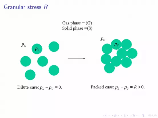
Granular stress R

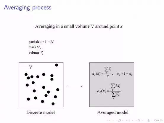
Averaging process

OutlinesTwo-phase granular flow models

Unstable one-pressure modelMore stable two-pressure modelEntropy and closure

Thermodynamically coherent granular stressShape of the granular stressEntropy and granular stress

Hyperbolicity studyStability of the relaxed systemInstability of the one-pressure model

Numerical approximation: splitting methodConvection stepRelaxation step

Numerical resultsStability studyCombustion chamber

Conclusion

Bibliography

Two-phase granular flow models

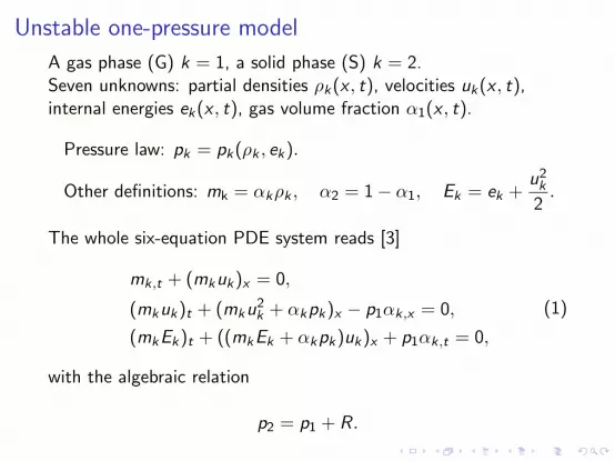
Unstable one-pressure model

A gas phase (G) k = 1, a solid phase (S) k = 2.Seven unknowns: partial densities ρk(x , t), velocities uk(x , t),internal energies ek(x , t), gas volume fraction α1(x , t).

Pressure law: pk = pk(ρk , ek).

Other definitions: mk = αkρk , α2 = 1− α1, Ek = ek +u2k

2.

The whole six-equation PDE system reads [3]

mk,t + (mkuk)x = 0,

(mkuk)t + (mku2k + αkpk)x − p1αk,x = 0,

(mkEk)t + ((mkEk + αkpk)uk)x + p1αk,t = 0,

(1)

with the algebraic relation

p2 = p1 + R.

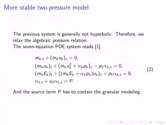
More stable two-pressure model

The previous system is generally not hyperbolic. Therefore, werelax the algebraic pressure relation.The seven-equation PDE system reads [1]

mk,t + (mkuk)x = 0,

(mkuk)t + (mku2k + αkpk)x − p1αk,x = 0,

(mkEk)t + ((mkEk + αkpk)uk)x + p1αk,t = 0,

α1,t + u2α1,x = P.

(2)

And the source term P has to contain the granular modeling.

Entropy and closureThe gas entropy s1 satisfies the standard relation (Tk is thetemperature of phase k)

T1ds1 = de1 −p1

ρ21

dρ1.

For the entropy s2 of the solid phase, we take into account thegranular stress.

T2ds2︸ ︷︷ ︸energy variation

= de2︸︷︷︸internal energy variation

−p2

ρ22

dρ2︸ ︷︷ ︸pressure work

− R

m2dα2︸ ︷︷ ︸

granular work

After some computations, we find the following entropy dissipationequation

(∑k

mksk)t + (∑k

mkuksk)x =P

T2(p1 + R − p2) .

A natural choice that ensures positive dissipation is

P =1

τpα1α2(p1 + R − p2), τp > 0 .

The choice of the pressure relaxation parameter τp is veryimportant. We can also write

p1 + R − p2 =τpα1α2

(α1,t + u2α1,x) .

I for τp = teq = 0, we recover the instantaneous six-equationequilibrium model p2 = p1 + R;

I τp = teqpref where teq is the characteristic time of thepressure equilibrium and pref a reference pressure;

I for τp > 0, the system should be more stable.

Thermodynamically coherent granular stress

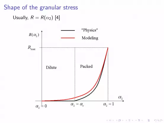
Shape of the granular stress

Usually, R = R(α2) [4]

Entropy and granular stress

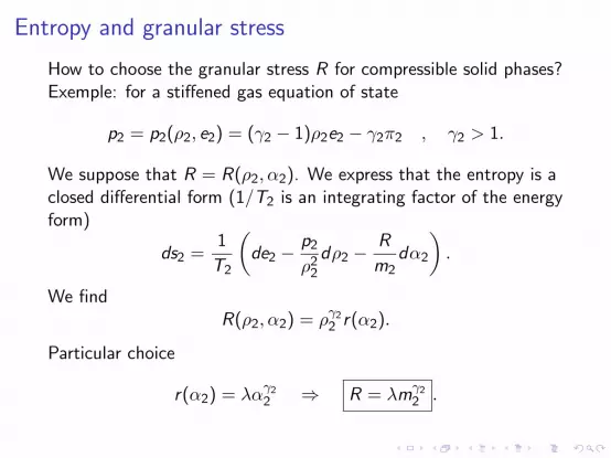
How to choose the granular stress R for compressible solid phases?Exemple: for a stiffened gas equation of state

p2 = p2(ρ2, e2) = (γ2 − 1)ρ2e2 − γ2π2 , γ2 > 1.

We suppose that R = R(ρ2, α2). We express that the entropy is aclosed differential form (1/T2 is an integrating factor of the energyform)

ds2 =1

T2

(de2 −

p2

ρ22

dρ2 −R

m2dα2

).

We findR(ρ2, α2) = ργ2

2 r(α2).

Particular choice

r(α2) = λαγ22 ⇒ R = λmγ2

2 .

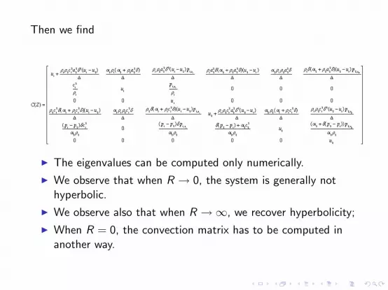
Hyperbolicity study

Stability of the relaxed system (τp > 0)

LetY = (α1, ρ1, u1, s1, ρ2, u2, s2)T .

In this set of variables the system becomes

Yt + B(Y )Yx = (P, 0, 0, 0, 0, 0, 0)T

B(Y ) =

u2ρ1(u1−u2)

α1u1 ρ1

c21

ρ1u1

p1,s1

ρ1

u1

u2 ρ2

p1−p2

m2

c22

ρ2u2

p2,s2

ρ2

u2

, ck =

√γk(pk + πk)

ρk.

det(B(Y )−λI ) = (u2−λ)2(u1−λ)(u1−c1−λ)(u1+c1−λ)(u2−c2−λ)(u2+c2−λ).

The system is hyperbolic [6, 2].

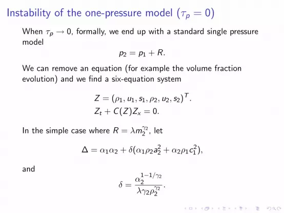
Instability of the one-pressure model (τp = 0)

When τp → 0, formally, we end up with a standard single pressuremodel

p2 = p1 + R.

We can remove an equation (for example the volume fractionevolution) and we find a six-equation system

Z = (ρ1, u1, s1, ρ2, u2, s2)T .

Zt + C (Z )Zx = 0.

In the simple case where R = λmγ22 , let

∆ = α1α2 + δ(α1ρ2a22 + α2ρ1c

21 ),

and

δ =α

1−1/γ2

2

λγ2ργ22

.

Then we find

I The eigenvalues can be computed only numerically.

I We observe that when R → 0, the system is generally nothyperbolic.

I We observe also that when R →∞, we recover hyperbolicity;

I When R = 0, the convection matrix has to be computed inanother way.

Numerical approximation: splitting method

I The two-pressure model is hyperbolic and more stable.

I The one-pressure model is commonly used in applications oncoarse meshes (high damping of the numerical viscosity).

I We can approximate the one-pressure model by the moregeneral two-pressure model.

I A time step is made of a convection stage and a relaxationstage. In the relaxation stage, we apply the exact or relaxedpressure equilibrium.

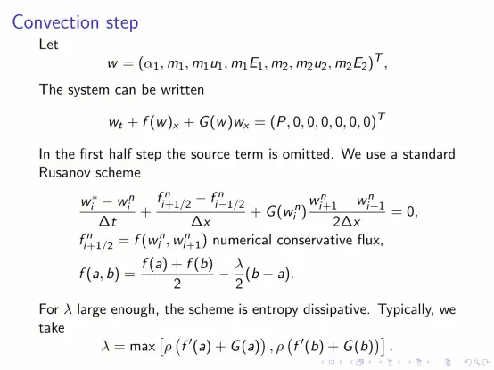
Convection stepLet

w = (α1,m1,m1u1,m1E1,m2,m2u2,m2E2)T ,

The system can be written

wt + f (w)x + G (w)wx = (P, 0, 0, 0, 0, 0, 0)T

In the first half step the source term is omitted. We use a standardRusanov scheme

w∗i − wni

∆t+

f ni+1/2 − f n

i−1/2

∆x+ G (wn

i )wn

i+1 − wni−1

2∆x= 0,

f ni+1/2 = f (wn

i ,wni+1) numerical conservative flux,

f (a, b) =f (a) + f (b)

2− λ

2(b − a).

For λ large enough, the scheme is entropy dissipative. Typically, wetake

λ = max[ρ(f ′(a) + G (a)

), ρ(f ′(b) + G (b)

)].

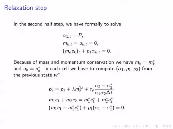
Relaxation step

In the second half step, we have formally to solve

α1,t = P,

mk,t = uk,t = 0,

(mkek)t + p1αk,t = 0.

Because of mass and momentum conservation we have mk = m∗kand uk = u∗k . In each cell we have to compute (α1, p1, p2) fromthe previous state w∗

p2 = p1 + λmγ22 + τp

α2 − α∗2α1α2∆t

,

m1e1 + m2e2 = m∗1e∗1 + m∗2e

∗2 ,

(m1e1 −m∗1e∗1 ) + p1(α1 − α∗1) = 0.

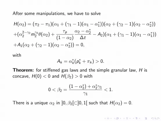
After some manipulations, we have to solve

H(α2) = (π2 − π1)(α1 + (γ1 − 1)(α1 − α∗1))(α2 + (γ2 − 1)(α2 − α∗2))

+(α2−γ22 mγ2

2 θ(α2) +τp

(1− α2)

α2 − α∗2∆t

− A2)(α1 + (γ1 − 1)(α1 − α∗1))

+A1(α2 + (γ2 − 1)(α2 − α∗2)) = 0,

withAk = α∗k(p∗k + πk) > 0.

Theorem: for stiffened gas laws and the simple granular law, H isconcave, H(0) < 0 and H(β2) > 0 with

0 < β2 =(1− α∗2) + α∗2γ1

γ1< 1.

There is a unique α2 in ]0, β2[⊂]0, 1[ such that H(α2) = 0.

Numerical application

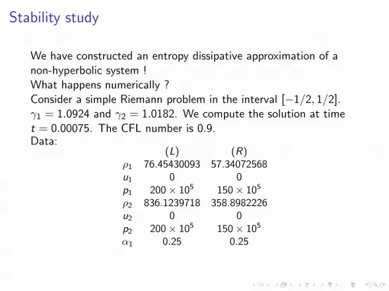
Stability study

We have constructed an entropy dissipative approximation of anon-hyperbolic system !What happens numerically ?Consider a simple Riemann problem in the interval [−1/2, 1/2].γ1 = 1.0924 and γ2 = 1.0182. We compute the solution at timet = 0.00075. The CFL number is 0.9.Data:

(L) (R)ρ1 76.45430093 57.34072568u1 0 0p1 200× 105 150× 105

ρ2 836.1239718 358.8982226u2 0 0p2 200× 105 150× 105

α1 0.25 0.25

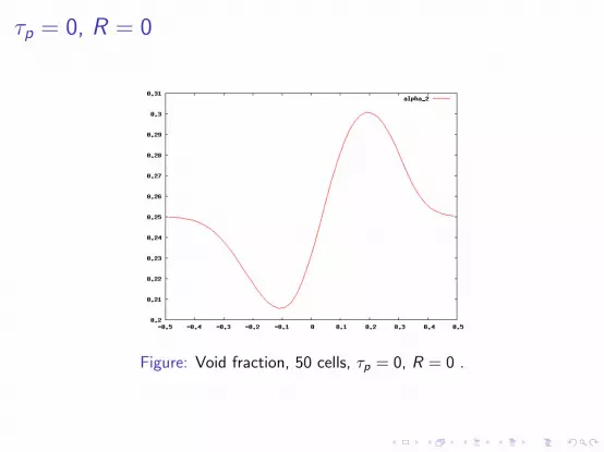
τp = 0, R = 0

Figure: Void fraction, 50 cells, τp = 0, R = 0 .

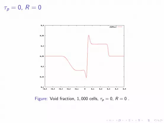
τp = 0, R = 0

Figure: Void fraction, 1, 000 cells, τp = 0, R = 0 .

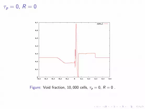
τp = 0, R = 0

Figure: Void fraction, 10, 000 cells, τp = 0, R = 0 .

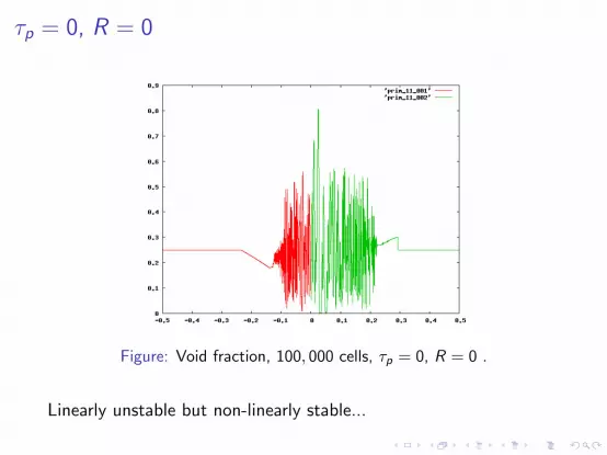
τp = 0, R = 0

Figure: Void fraction, 100, 000 cells, τp = 0, R = 0 .

Linearly unstable but non-linearly stable...

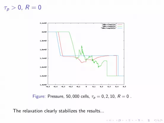
τp > 0, R = 0

Figure: Pressure, 50, 000 cells, τp = 0, 2, 10, R = 0 .

The relaxation clearly stabilizes the results...

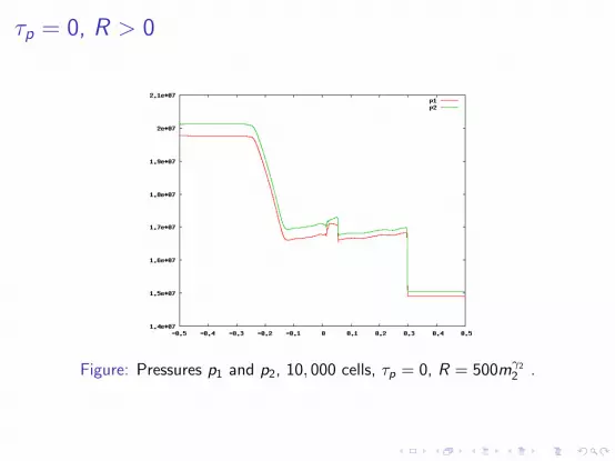
τp = 0, R > 0

Figure: Pressures p1 and p2, 10, 000 cells, τp = 0, R = 500mγ2

2 .

τp = 0, R > 0

Figure: Eigenvalues: imaginary part I =

√6∑

i=1

Im (λi )2, 1, 000 cells,

R = 0 or R = 500mγ2

2 .

The granular stress slightly improves the stability...

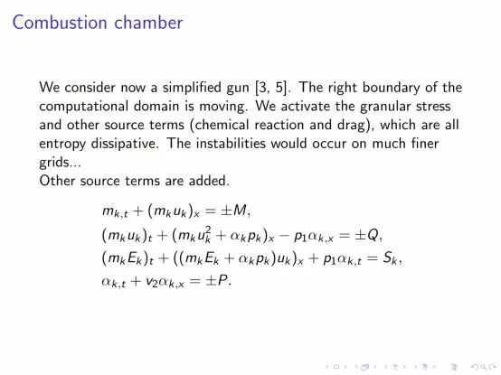
Combustion chamber

We consider now a simplified gun [3, 5]. The right boundary of thecomputational domain is moving. We activate the granular stressand other source terms (chemical reaction and drag), which are allentropy dissipative. The instabilities would occur on much finergrids...Other source terms are added.

mk,t + (mkuk)x = ±M,

(mkuk)t + (mku2k + αkpk)x − p1αk,x = ±Q,

(mkEk)t + ((mkEk + αkpk)uk)x + p1αk,t = Sk ,

αk,t + v2αk,x = ±P.

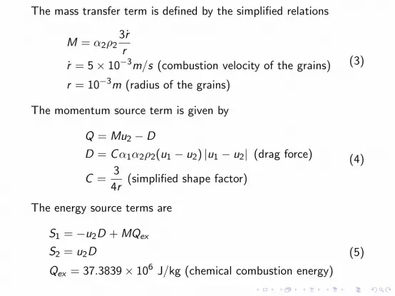
The mass transfer term is defined by the simplified relations

M = α2ρ23r

rr = 5× 10−3m/s (combustion velocity of the grains)

r = 10−3m (radius of the grains)

(3)

The momentum source term is given by

Q = Mu2 − D

D = Cα1α2ρ2(u1 − u2) |u1 − u2| (drag force)

C =3

4r(simplified shape factor)

(4)

The energy source terms are

S1 = −u2D + MQex

S2 = u2D

Qex = 37.3839× 106 J/kg (chemical combustion energy)

(5)

Figure: Pressure evolution at the breech and the shot base during time.Comparison between the Gough and the relaxation model.

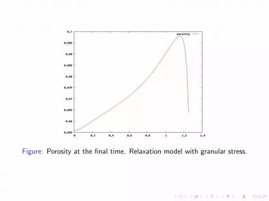
Figure: Porosity at the final time. Relaxation model with granular stress.

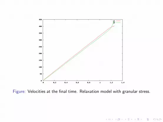
Figure: Velocities at the final time. Relaxation model with granular stress.

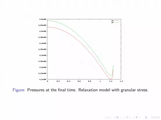
Figure: Pressures at the final time. Relaxation model with granular stress.

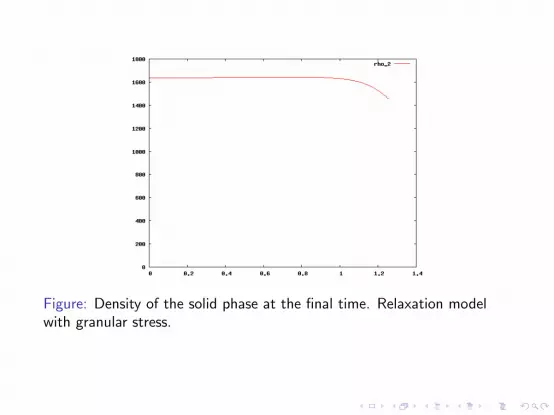
Figure: Density of the solid phase at the final time. Relaxation modelwith granular stress.

Conclusion

I Good generalization of the one pressure models;

I Extension of the relaxation approach to flows with granularstress;

I Rigorous entropy dissipation and maximum principle on thevolume fraction;

I Stability for a finite relaxation time;

I The instability is (fortunately) preserved by the scheme forfast pressure equilibrium;

I The model can be used in practical configurations (the solidphase remains almost incompressible).

Bibliography

M. R. Baer and J. W. Nunziato.

A two phase mixture theory for the deflagration to detonation transition (ddt) in reactive granular materials.Int. J. for Multiphase Flow, 16(6):861–889, 1986.

Thierry Gallouet, Jean-Marc Herard, and Nicolas Seguin.

Numerical modeling of two-phase flows using the two-fluid two-pressure approach.Math. Models Methods Appl. Sci., 14(5):663–700, 2004.

P. S. Gough.

Modeling of two-phase flows in guns.AIAA, 66:176–196, 1979.

A. K. Kapila, R. Menikoff, J. B. Bdzil, S. F. Son, and D. S. Stewart.

Two-phase modeling of deflagration-to-detonation transition in granular materials: reduced equations.Physics of Fluids, 13(10):3002–3024, 2001.

Julien Nussbaum, Philippe Helluy, Jean-Marc Herard, and Alain Carriere.

Numerical simulations of gas-particle flows with combustion.Flow, Turbulence and Combustion, 76(4):403–417, 2006.

R. Saurel and R. Abgrall.

A multiphase Godunov method for compressible multifluid and multiphase flows.Journal of Computational Physics, 150(2):425–467, 1999.