experimental study on interfacial area transport in bubbly two-phase flows

This is the author version of an article published as: Hibiki, Takashi and Situ, Rong and Mi, Ye and Ishii, Mamoru (2003) Experimental Study on Interfacial Area Transport in Vertical Upward Bubbly Two-Phase Flow in an Annulus. International Journal of Heat and Mass Transfer 46(3):pp. 427-441. Copyright 2003 Elsevier Accessed from http://eprints.qut.edu.au

http://eprints.qut.edu.au/

T. Hibiki et al. / Experimental Study of Interfacial Area Transport

1

Experimental Study on Interfacial Area Transport in

Vertical Upward Bubbly Two-Phase Flow in an Annulus

Takashi Hibiki a, b, *

, Rong Situ b, Ye Mi

b, Mamoru Ishii

b

a Research Reactor Institute, Kyoto University, Kumatori, Sennan, Osaka 590-0494, Japan

b School of Nuclear Engineering, Purdue University, West Lafayette, IN 47907-1290, USA

* Tel: +81-724-51-2373, Fax.: +81-724-51-2461, Email: [email protected]

Abstract

In relation to the development of the interfacial area transport equation, axial

developments of local void fraction, interfacial area concentration, and interfacial velocity of

vertical upward bubbly flows in an annulus with the hydraulic equivalent diameter of 19.1 mm

were measured by the double-sensor conductivity probe. A total of 20 data were acquired

consisting of five void fractions, about 0.050, 0.10, 0.15, 0.20, and 0.25, and four superficial

liquid velocities, 0.272, 0.516, 1.03, and 2.08 m/s. The obtained data will be used for the

development of reliable constitutive relations, which reflect the true transfer mechanisms in

subcooled boiling flow systems.

Key Words: Interfacial area transport; Two-fluid model; Void fraction, Interfacial area

concentration; Double-sensor conductivity probe; Gas-liquid bubbly flow; Multiphase flow


2

Nomenclature

ai interfacial area concentration

ai,0 interfacial area concentration at inlet

ai,eq. interfacial area concentration under conditions of no phase change and

equilibrium of bubble coalescence and breakup rates

D diameter of round tube

DH hydraulic equivalent diameter

DSm Sauter mean diameter

jg superficial gas velocity

jg,N superficial gas velocity reduced at normal condition (atmospheric pressure and 20°C)

jf superficial liquid velocity

n exponent

n0 asymptotic exponent at <α>=0

P pressure

P0 pressure at inlet

R radius of outer round tube

R0 radius of inner rod

Ref Reynolds number of liquid phase

r radial coordinate

rP radial coordinate at void peak

Sj sink or source term in the interfacial area concentration due to bubble coalescence or

breakup, respectively

Sph sink or source term in interfacial area concentration due to phase change


3

t time

vg interfacial velocity obtained by effective signals

z axial coordinate

Greek symbols

α void fraction

αC void fraction at channel center

αP void fraction at void peak

∆ρ density difference

νf kinetic viscosity of liquid phase

ξ interfacial area concentration change due to bubble coalescence or breakup

σ interfacial tension

ψ factor depending on bubble shape (1/(36π) for a spherical bubble)

Mathematical symbols

< > area-averaged quantity

<< >> void fraction weighted cross-sectional area-averaged quantity

<< >>a interfacial are concentration weighted cross-sectional area-averaged quantity

1. Introduction

In relation to the modeling of the interfacial transfer terms in the two-fluid model, the

concept of the interfacial area transport equation has recently been proposed to develop the

constitutive relation on the interfacial area concentration [1]. The interfacial area concentration

https://www.researchgate.net/publication/223370702_Foundation_of_the_Interfacial_Area_Transport_Equation_and_Its_Closure_Relation?el=1_x_8&enrichId=rgreq-58170fa3de37652cf17a03628cbe0f53-XXX&enrichSource=Y292ZXJQYWdlOzIyMjA2MzE2MjtBUzoxNTI5NzYzNTQxODkzMTVAMTQxMzQ4MzgxMzgxMw==


4

change can basically be characterized by the variation of the particle number density due to

coalescence and breakup of bubbles. The interfacial area transport equation can be derived by

considering the fluid particle number density transport equation analogous to Boltzmann’s

transport equation [1]. The interfacial area transport equation can replace the traditional flow

regime maps and regime transition criteria. The changes in the two-phase flow structure can be

predicted mechanistically by introducing the interfacial area transport equation. The effects of

the boundary conditions and flow development are efficiently modeled by this transport equation.

Such a capability does not exist in the current state-of-the-art nuclear thermal-hydraulic system

analysis codes like RELAP5, TRAC and CATHARE. Thus, a successful development of the

interfacial area transport equation can make a quantum improvement in the two-fluid model

formulation and the prediction accuracy of the system codes.

The strategy for the development of the interfacial area transport equation consists of (1)

formulation of the interfacial area transport equation, (2) development of measurement techniques

for local flow parameters, (3) construction of data base of axial development of local flow

parameters, (4) modeling of sink and source terms in the interfacial area transport equation, and

(5) improvement of thermal-hydraulic system analysis codes by implementing the interfacial area

transport equation. The present status of the above sub-divided projects was extensively

reviewed in the previous paper [2]. In the first stage of the development of the interfacial area

transport equation, adiabatic flow was the focus, and the interfacial area transport equation for the

adiabatic flow was developed successfully by modeling sink and source terms of the interfacial

area concentration due to bubble coalescence and breakup. In the next stage, subcooled boiling

flow would be the focus, and a preliminary local measurement for interfacial area concentration

was initiated for subcooled boiling water flow in an internally heated annulus [3]. To develop

https://www.researchgate.net/publication/27470389_Interfacial_area_measurements_in_subcooled_flow_boiling?el=1_x_8&enrichId=rgreq-58170fa3de37652cf17a03628cbe0f53-XXX&enrichSource=Y292ZXJQYWdlOzIyMjA2MzE2MjtBUzoxNTI5NzYzNTQxODkzMTVAMTQxMzQ4MzgxMzgxMw==

https://www.researchgate.net/publication/263256525_Development_of_one-group_interfacial_area_transport_equation_in_bubbly_flow_systems?el=1_x_8&enrichId=rgreq-58170fa3de37652cf17a03628cbe0f53-XXX&enrichSource=Y292ZXJQYWdlOzIyMjA2MzE2MjtBUzoxNTI5NzYzNTQxODkzMTVAMTQxMzQ4MzgxMzgxMw==



5

the interfacial area transport equation for boiling flows in the internally heated annulus, sink and

source terms due to phase change should be modeled based on rigorous and extensive boiling

flow data to be taken in the annular channel, and sink and source terms due to bubble coalescence

and breakup modeled previously should be evaluated separately based on adiabatic data to be

taken in the same channel. If necessary, previously modeled sink and source terms [2] should be

modified.

From this point of view, this study aims at measuring axial development of local flow

parameters of vertical upward air-water bubbly flows in an annulus by using a double-sensor

conductivity probe. The annulus test loop is scaled to a prototypic BWR based on scaling

criteria for geometric, hydrodynamic, and thermal similarities [3]. It consists of an inner rod

with a diameter of 19.1 mm and an outer round tube with an inner diameter of 38.1 mm, and the

hydraulic equivalent diameter is 19.1 mm. Measured flow parameters include void fraction,

interfacial area concentration, and interfacial velocity. A total of 20 data sets are acquired

consisting of five void fractions, about 0.050, 0.10, 0.15, 0.20, and 0.25, and four superficial

liquid velocities, 0.272, 0.516, 1.03, and 2.08 m/s. The measurements for each flow condition

are performed at the four axial locations: axial locations non-dimensionalized by the hydraulic

equivalent diameter = 40.3, 61.7, 77.7, and 99.0. The data obtained from the double-sensor

conductivity probe give near complete information on the time-averaged local hydrodynamic

parameters of bubbly flow to model the sink and source terms of the interfacial area concentration.

The data set obtained in this study will eventually be used for the development of reliable

constitutive relations, which reflect the true transfer mechanisms in subcooled boiling flow

systems.




6

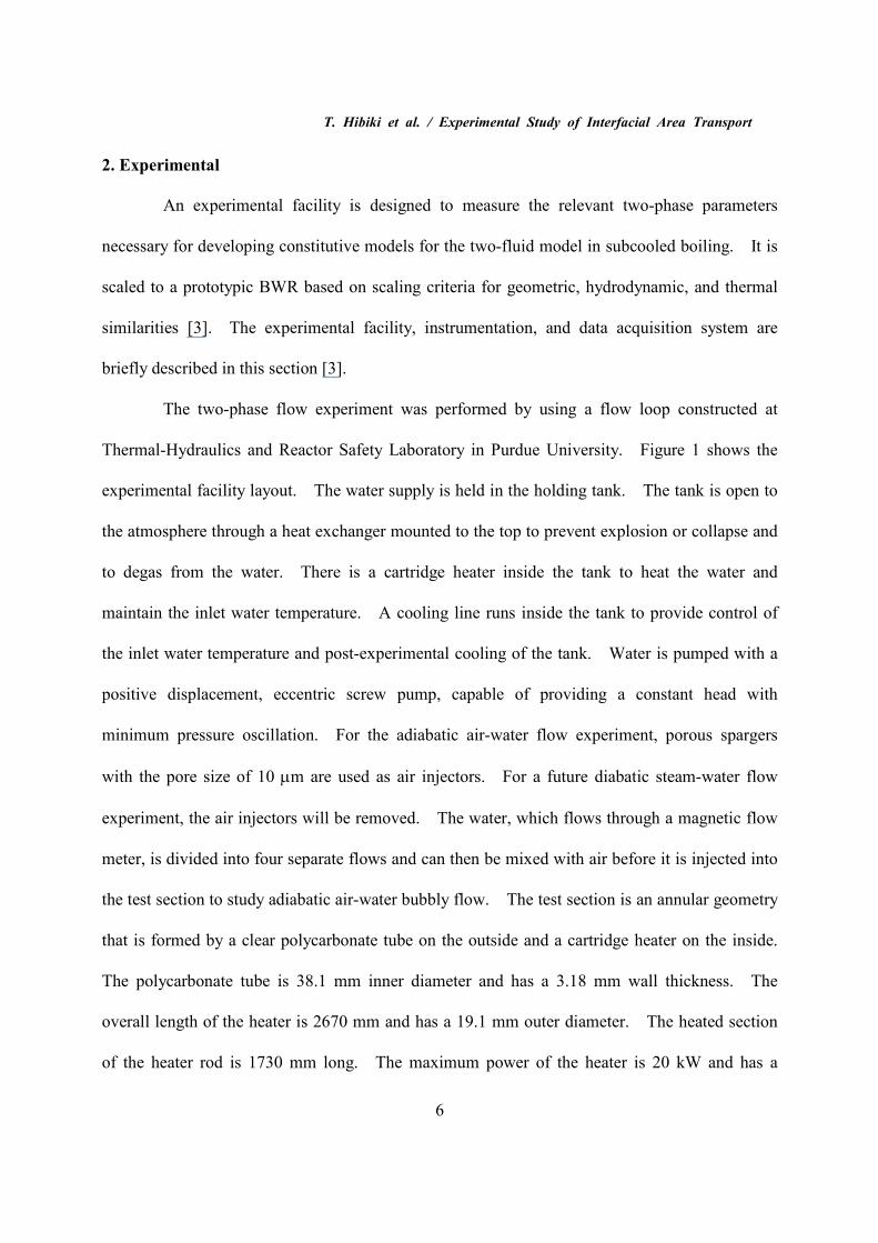
2. Experimental

An experimental facility is designed to measure the relevant two-phase parameters

necessary for developing constitutive models for the two-fluid model in subcooled boiling. It is

scaled to a prototypic BWR based on scaling criteria for geometric, hydrodynamic, and thermal

similarities [3]. The experimental facility, instrumentation, and data acquisition system are

briefly described in this section [3].

The two-phase flow experiment was performed by using a flow loop constructed at

Thermal-Hydraulics and Reactor Safety Laboratory in Purdue University. Figure 1 shows the

experimental facility layout. The water supply is held in the holding tank. The tank is open to

the atmosphere through a heat exchanger mounted to the top to prevent explosion or collapse and

to degas from the water. There is a cartridge heater inside the tank to heat the water and

maintain the inlet water temperature. A cooling line runs inside the tank to provide control of

the inlet water temperature and post-experimental cooling of the tank. Water is pumped with a

positive displacement, eccentric screw pump, capable of providing a constant head with

minimum pressure oscillation. For the adiabatic air-water flow experiment, porous spargers

with the pore size of 10 µm are used as air injectors. For a future diabatic steam-water flow

experiment, the air injectors will be removed. The water, which flows through a magnetic flow

meter, is divided into four separate flows and can then be mixed with air before it is injected into

the test section to study adiabatic air-water bubbly flow. The test section is an annular geometry

that is formed by a clear polycarbonate tube on the outside and a cartridge heater on the inside.

The polycarbonate tube is 38.1 mm inner diameter and has a 3.18 mm wall thickness. The

overall length of the heater is 2670 mm and has a 19.1 mm outer diameter. The heated section

of the heater rod is 1730 mm long. The maximum power of the heater is 20 kW and has a




7

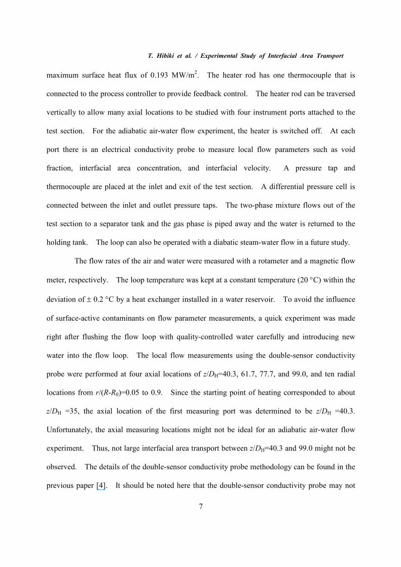
maximum surface heat flux of 0.193 MW/m2. The heater rod has one thermocouple that is

connected to the process controller to provide feedback control. The heater rod can be traversed

vertically to allow many axial locations to be studied with four instrument ports attached to the

test section. For the adiabatic air-water flow experiment, the heater is switched off. At each

port there is an electrical conductivity probe to measure local flow parameters such as void

fraction, interfacial area concentration, and interfacial velocity. A pressure tap and

thermocouple are placed at the inlet and exit of the test section. A differential pressure cell is

connected between the inlet and outlet pressure taps. The two-phase mixture flows out of the

test section to a separator tank and the gas phase is piped away and the water is returned to the

holding tank. The loop can also be operated with a diabatic steam-water flow in a future study.

The flow rates of the air and water were measured with a rotameter and a magnetic flow

meter, respectively. The loop temperature was kept at a constant temperature (20 °C) within the

deviation of ± 0.2 °C by a heat exchanger installed in a water reservoir. To avoid the influence

of surface-active contaminants on flow parameter measurements, a quick experiment was made

right after flushing the flow loop with quality-controlled water carefully and introducing new

water into the flow loop. The local flow measurements using the double-sensor conductivity

probe were performed at four axial locations of z/DH=40.3, 61.7, 77.7, and 99.0, and ten radial

locations from r/(R-R0)=0.05 to 0.9. Since the starting point of heating corresponded to about

z/DH =35, the axial location of the first measuring port was determined to be z/DH =40.3.

Unfortunately, the axial measuring locations might not be ideal for an adiabatic air-water flow

experiment. Thus, not large interfacial area transport between z/DH=40.3 and 99.0 might not be

observed. The details of the double-sensor conductivity probe methodology can be found in the

previous paper [4]. It should be noted here that the double-sensor conductivity probe may not

https://www.researchgate.net/publication/229126005_Development_of_the_miniaturized_four-sensor_conductivity_probe_and_the_signal_processing_scheme?el=1_x_8&enrichId=rgreq-58170fa3de37652cf17a03628cbe0f53-XXX&enrichSource=Y292ZXJQYWdlOzIyMjA2MzE2MjtBUzoxNTI5NzYzNTQxODkzMTVAMTQxMzQ4MzgxMzgxMw==


8

work for the interfacial area concentration and interfacial velocity measurements in the vicinity of

the wall. The data of the interfacial area concentration and interfacial velocity in the vicinity of

the wall can be corrected by assuming the power-law profile of the interfacial velocity. The

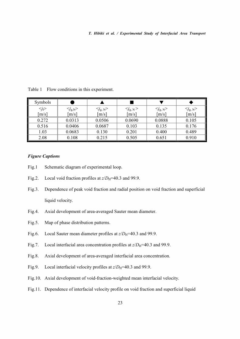
details of the correction method can be found in the previous paper [5]. The flow conditions in

this experiment are tabulated in Table 1. The area-averaged superficial gas velocities in this

experiment were roughly determined so as to provide the same area-averaged void fractions

among different conditions of superficial liquid velocity, namely <α>=0.050, 0.10, 0.15, 0.20,

and 0.25.

In order to verify the accuracy of local measurements, the area-averaged quantities

obtained by integrating the local flow parameters over the flow channel were compared with

those measured by other cross-calibration methods such as a γ-densitometer for void fraction, a

photographic method for interfacial area concentration, and a rotameter for superficial gas

velocity. Good agreements were obtained between the area-averaged void fraction, interfacial

area concentration and superficial gas velocity obtained from the local measurements and those

measured by the γ-densitometer, the photographic method and the rotameter with averaged

relative deviations of ±12.8, ±6.95 and ±12.9 %, respectively [5]. The benchmark

experiments for the double-sensor probe were also performed in an acrylic vertical rectangular

flow duct in air-water two-phase mixture. Local flow parameters measured by an image

processing method were compared with those by the double-sensor probe methods. The relative

percent difference between the two methods was within ±10 % [4]. Based on these results, it

can be thought that the measurement accuracy of local flow parameters would be within ±10 %.

3. Results and Discussion

https://www.researchgate.net/publication/229126005_Development_of_the_miniaturized_four-sensor_conductivity_probe_and_the_signal_processing_scheme?el=1_x_8&enrichId=rgreq-58170fa3de37652cf17a03628cbe0f53-XXX&enrichSource=Y292ZXJQYWdlOzIyMjA2MzE2MjtBUzoxNTI5NzYzNTQxODkzMTVAMTQxMzQ4MzgxMzgxMw==


9

3.1. Local Flow Parameters

3.1.1. Phase distribution pattern

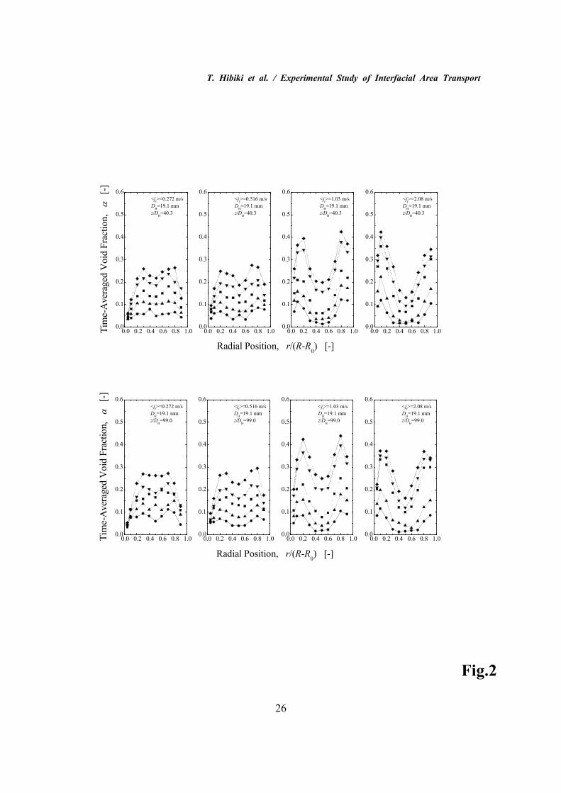
Figure 2 shows the behavior of void fraction profiles measured at z/DH=40.3 (upper

figures) and 99.0 (lower figures) in this experiment. The meanings of the symbols in Fig.2 are

found in Table 1. As can be seen from Fig.2, various phase distribution patterns similar to those

in round tubes were observed in the present experiment, and void fraction profiles were found to

be almost symmetrical with respect to the channel center, r/(R-R0)=0.5. Significant differences

between the phase distributions at z/DH=40.3 and 99.0 were not observed. The phase

distribution patterns may be governed by the flow field and the bubble size. The bubble size is

governed by the interfacial area transport due to bubble coalescence, breakup, expansion and

shrinkage. The interfacial area transport stages may roughly be classified into three stages such

as (1) the interfacial area transport governed by coalescence and breakup of primary bubbles near

a test section inlet, (2) the interfacial area transport governed by coalescence and breakup of

secondary bubbles and (3) the interfacial area transport governed by bubble expansion or

shrinkage where bubble breakup and coalescence come to be an equilibrium state. According to

previous experimental results in round tubes [6, 7], significant interfacial area transport occurred

in the stage (1) (z/DH ≤ 15) and gradual interfacial area transport occurred in the stage (2) (15 <

z/DH ≤ 60). Thus, it can be thought that the flow in the annulus almost reached to a quasi

fully-developed flow.

Serizawa and Kataoka classified the phase distribution pattern into four basic types of

the distributions, that is, “wall peak”, “intermediate peak”, “core peak”, and “transition” [8].

The wall peak is characterized as sharp peak with relatively high void fraction near the channel

wall and plateau with very low void fraction around the channel center. The intermediate peak

https://www.researchgate.net/publication/223861195_Axial_Interfacial_Area_Transport_of_Vertical_Bubbly_Flows?el=1_x_8&enrichId=rgreq-58170fa3de37652cf17a03628cbe0f53-XXX&enrichSource=Y292ZXJQYWdlOzIyMjA2MzE2MjtBUzoxNTI5NzYzNTQxODkzMTVAMTQxMzQ4MzgxMzgxMw==

https://www.researchgate.net/publication/222842931_Experimental_Study_on_Interfacial_Area_Transport_in_Bubbly_Two-Phase_Flows?el=1_x_8&enrichId=rgreq-58170fa3de37652cf17a03628cbe0f53-XXX&enrichSource=Y292ZXJQYWdlOzIyMjA2MzE2MjtBUzoxNTI5NzYzNTQxODkzMTVAMTQxMzQ4MzgxMzgxMw==


10

is explained as broad peak in void fraction near the channel wall and plateau with medium void

fraction around the channel center. The core peak is defined as broad peak around the channel

center and no peak near the channel wall. The transition is described as two broad peaks around

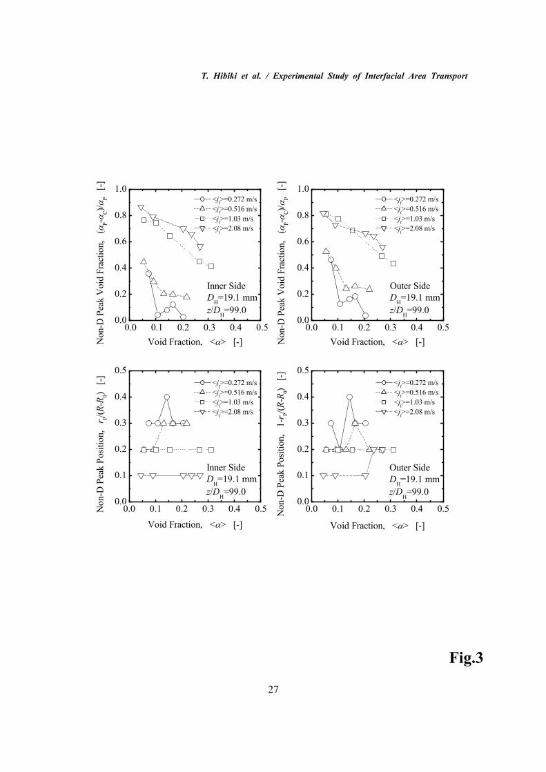
the channel wall and center. In Fig.3, non-dimensional peak void fraction (upper figures) and

peak radial position (lower figures) measured at z/DH=99.0 are plotted against the area-averaged

void fraction as a parameter of the superficial liquid velocity. The non-dimensional void

fraction at the peak is defined as (αP-αC)/αP, where αP and αC are the void fractions at the peak

and the channel center, respectively. (αP-αC)/αP=0 and 1 indicate no wall peak and very sharp

wall peak, respectively. The non-dimensional radial position at the peak is defined as rP/(R-R0)

or 1-rP/(R-R0) for the peak appeared at inner side (r/(R-R0)≤0.5) or outer side (r/(R-R0)≥0.5) of the

channel, respectively, where rP is the peak radial position. It should be noted here that there is

uncertainty of one radial step in the peak position and the resulting uncertainty in peak void

fraction. However, an approximate trend on the effect of the non-dimensional peak void

fraction and the non-dimensional peak position on the area-averaged void fraction can be

observed in Fig.3.

As the superficial liquid velocity increased, the radial position at the void fraction peak

was moved towards the channel wall. The increase in the superficial liquid velocity also

augmented the void fraction at the peak and made the void fraction peak sharp. On the other

hand, in the present experimental condition, the increase in the void fraction did not change the

radial position at the void fraction peak significantly, and decreased the non-dimensional void

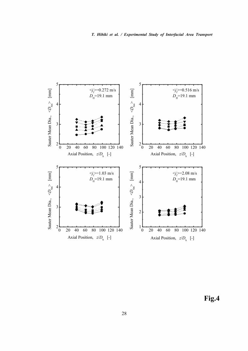
fraction at the peak, resulting in the broad void fraction peak. As general trends observed in the

present experiment, the increase in the superficial liquid velocity decreased the bubble size,

whereas the increase in the void fraction increased the bubble size, see Fig.4. In Fig.4, the


11

bracket of < > means the area-averaged quantity. It was pointed out that the bubble size and

liquid velocity profile would affect the void fraction distribution. Similar phenomena were also

observed by Sekoguchi et al. [9], Zun [10], and Serizawa and Kataoka [8]. Sekoguchi et al. [9]

observed the behaviors of isolated bubbles, which were introduced into vertical water flow in a

25 mm × 50 mm rectangular channel through a single nozzle. Based on their observations, they

found that the bubble behaviors in dilute suspension flow might depend on the bubble size and

the bubble shape. In their experiment, only distorted ellipsoidal bubbles with a diameter smaller

than nearly 5 mm tended to migrate toward the wall, whereas distorted ellipsoidal bubbles with a

diameter larger than 5 mm and spherical bubbles rose in the channel center. On the other hand,

for the water velocity lower than 0.3 m/s, no bubbles were observed in the wall region. Zun [10]

also obtained a similar result. Zun performed an experiment to study void fraction radial

profiles in upward vertical bubbly flow at very low average void fractions, around 0.5 %. In his

experiment, the wall void peaking flow regime existed both in laminar and turbulent bulk liquid

flow. The experimental results on turbulent bulk liquid flow at Reynolds number near 1000

showed distinctive higher bubble concentration at the wall region if the bubble equivalent sphere

diameter appeared in the range of 0.8 and 3.6 mm. Intermediate void profiles were observed at

bubble sizes either between 0.6 and 0.8 mm or 3.6 and 5.1 mm. Bubbles smaller than 0.6 mm or

larger than 5.1 mm tended to migrate towards at the channel center. Thus, these experimental

results suggested that the bubble size would play a dominant role in void fraction profiles.

Serizawa and Kataoka [8] also gave an extensive review on the bubble behaviors in bubbly-flow

regime.

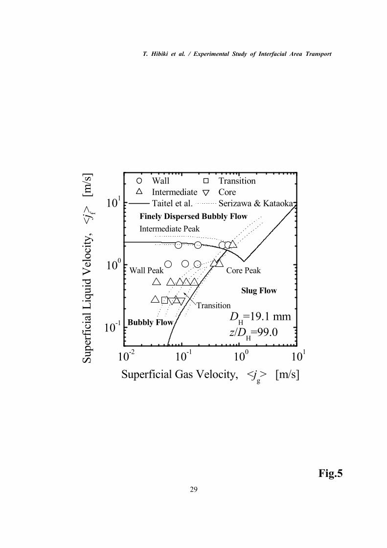
Figure 5 shows a map of phase distribution patterns observed at z/DH=99.0 in this

experiment. The open symbols of circle, triangle, square, and reversed triangle in Fig.5 indicate


12

the wall peak, the intermediate peak, the transition, and the core peak, respectively. Since

Serizawa and Kataoka [8] did not give the quantitative definitions of the wall and intermediate

peaks, the classification between the wall and intermediate peaks in the present study were

performed as the wall peak for (αP-αC)/αP≥0.5 and the intermediate peak for (αP-αC)/αP<0.5.

The solid and broken lines in Fig.5 are, respectively, the flow regime transition boundaries

predicted by the model of Taitel et al. [11] and the phase distribution pattern transition boundaries,

which were developed by Serizawa and Kataoka [8] based on experiments performed by different

researchers with different types of bubble injections in round tubes (20 mm ≤ D ≤ 86.4 mm).

Phase distribution patterns observed at z/DH=99.0 did not agree with the Serizawa-Kataoka’s map

[8] at low superficial liquid velocities. As can be seen from Fig.2, the void fraction profiles for

<jf>=0.272 m/s, were almost uniform along the radius with relatively steep decrease in the void

fraction close to wall. This may be attributed to strong mixing due to bubble-induced turbulence,

since it would dominate the flow in such a low flow condition. The strong mixing and partly

recirculation would make the void fraction profile flatter. The similar void fraction peak was

observed in the previous experiment using a 50.8 mm diameter pipe [7]. In the experiment, for

<jf>=5.00 m/s, not the intermediate peak suggested by the Serizawa-Kataoka’s map [8] but the

flat peak characterized as uniform void fraction profile along the channel radius with relatively

steep decrease in the void fraction near the wall was observed. The shear-induced turbulence

would dominate the flow in such a high flow condition. It was considered that the reason for the

phase distribution might be due to a strong bubble mixing over the flow channel by a strong

turbulence. Thus, low and high liquid velocity regions may be considered to be bubble-mixing

dominant zone, where the void fraction profile is uniform along the channel radius with relatively

steep decrease in the void fraction near the wall. Thus, based on the phase distribution pattern,


https://www.researchgate.net/publication/229928111_Modeling_Flow_Pattern_Transitions_for_Steady_Upward_Gas-Liquid_Flow_in_Vertical_Tubes?el=1_x_8&enrichId=rgreq-58170fa3de37652cf17a03628cbe0f53-XXX&enrichSource=Y292ZXJQYWdlOzIyMjA2MzE2MjtBUzoxNTI5NzYzNTQxODkzMTVAMTQxMzQ4MzgxMzgxMw==


13

bubbly flow region may be divided into four regions: (1) bubble-mixing region where the

bubble-induced turbulence is dominant, (2) region where the wall peak appears, (3) region where

the core peak appears, and (4) bubble-mixing region where the shear-induced turbulence is

dominant. The regions (1), (2), (3), and (4) are roughly located at low void fraction and low

liquid velocity (<α>≤0.25, <jf>≤0.3 m/s), low void fraction and medium liquid velocity

(<α>≤0.25, 0.3 m/s≤<jf>≤5 m/s), high void fraction (<α>≥0.25), and low void fraction and high

liquid velocity(<α>≤0.25, <jf>≥5 m/s), respectively. Various transition phase distribution

patterns would obviously appear between two regions. Intermediate peak and transition

categorized by Serizawa and Kataoka may just be the transition between regions (4) and (2) or (3),

and the transition between regions (1) and (2) or (3), respectively.

3.1.2. Void fraction

As described, significant differences between the phase distributions at z/DH=40.3 and

99.0 were not observed, since the flow might almost reach to a quasi fully-developed flow at

z/DH=40.3. However, some changes in void fraction profiles may be noted as follows. As

shown in Fig.2, for <jf>=0.272 m/s, broad core peak with plateau around the channel center and

intermediate peak were found for low (●,▲) and high (■,▼,◆) void fraction regions,

respectively, at the first measuring station of z/DH=40.3. As the flow developed, the plateau

observed for low void fraction region (●,▲) tended to be narrower. On the other hand, as the

flow developed, two peaks observed for high void fraction region (■,▼,◆) tended to move

towards the channel center and to be merged into one core peak. For <jf>=0.516 m/s,

intermediate peak was observed at the first measuring station of z/DH=40.3. As the flow

developed, the void fraction profiles were not changed for low void fraction region (●,▲), but


14

the trough of the void fraction profiles observed around the channel center came to be shallower

for high void fraction region (■,▼,◆). The similar tendency was observed for <jf>=1.03 m/s.

For <jf>=2.08 m/s, wall peak was observed at the first measuring station of z/DH=40.3. As the

flow developed, the void fraction profiles were not changed. For <jf>=0.272, 0.516, and 1.03

m/s, the bubble diameter was about 3 mm, which was close to a critical bubble size of 3.6 mm

pointed out by Zun [10], which gave the boundary between the wall and intermediate peaks.

The bubble size was likely to determine the direction of the bubble migration. Thus, in these

cases, bubbles tended to move towards the channel center gradually. For <jf>=2.08 m/s, the

bubble diameter was about 2 mm, enabled the bubbles to stay near the channel wall, resulting in

insignificant axial change of the void fraction distribution.

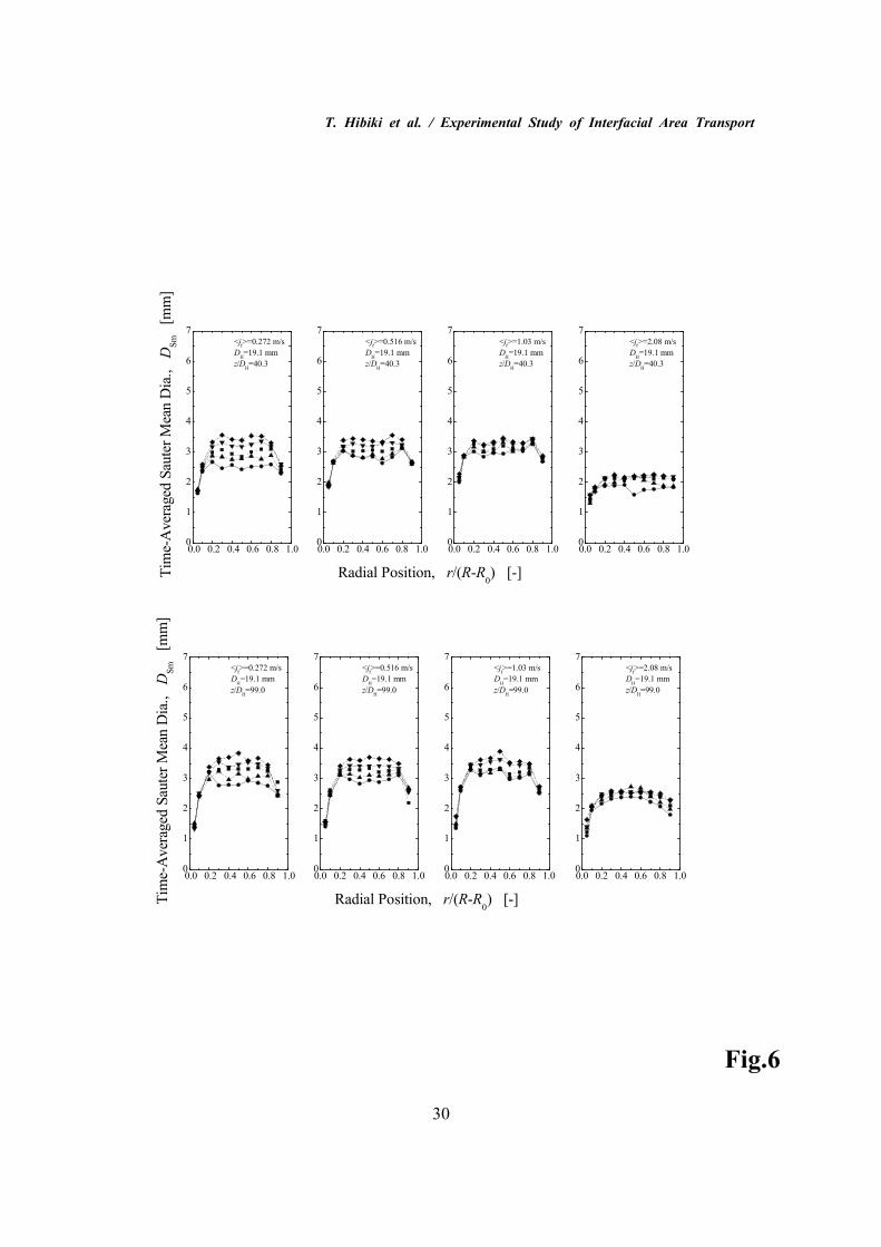
3.1.3. Sauter mean diameter

Figure 6 shows the behavior of Sauter mean diameter profiles, corresponding to that of

void fraction profiles in Fig.2. Figure 4 also shows the axial development of area-averaged

Sauter mean diameters, <DSm>, obtained by the area-averaged void fraction and interfacial area

concentration with <DSm>=6<α>/<ai>. The meanings of the symbols in Figs.4 and 6 are found

in Table 1. The Sauter mean diameter profiles were almost uniform along the channel radius

with some decrease in size near the wall, r/(R-R0)≤0.1 and 0.9≤r/(R-R0). Only a part of a bubble

can pass the region close to the channel wall, resulting in apparent small Sauter mean diameter.

The profiles were not changed significantly as the flow developed, although the bubble size

increased up to 10-20 % along the flow direction mainly due to the bubble expansion (see Fig.6).

3.1.4. Interfacial area concentration

Figure 7 shows the behavior of interfacial area concentration profiles, corresponding to

that of void fraction profiles in Fig.2. Figure 8 also shows the axial development of


15

area-averaged interfacial area concentrations, <ai>, obtained by integrating local interfacial area

concentration over the flow channel. The meanings of the symbols in Figs.7 and 8 are found in

Table 1. As expected for bubbly flow, the interfacial area concentration profiles were similar to

the void fraction profiles. Since the interfacial area concentration would directly be proportional

to the void fraction and the Sauter mean diameter was almost uniform along the channel radius,

the interfacial area concentration profiles displayed the same behavior as their respective void

fraction profiles.

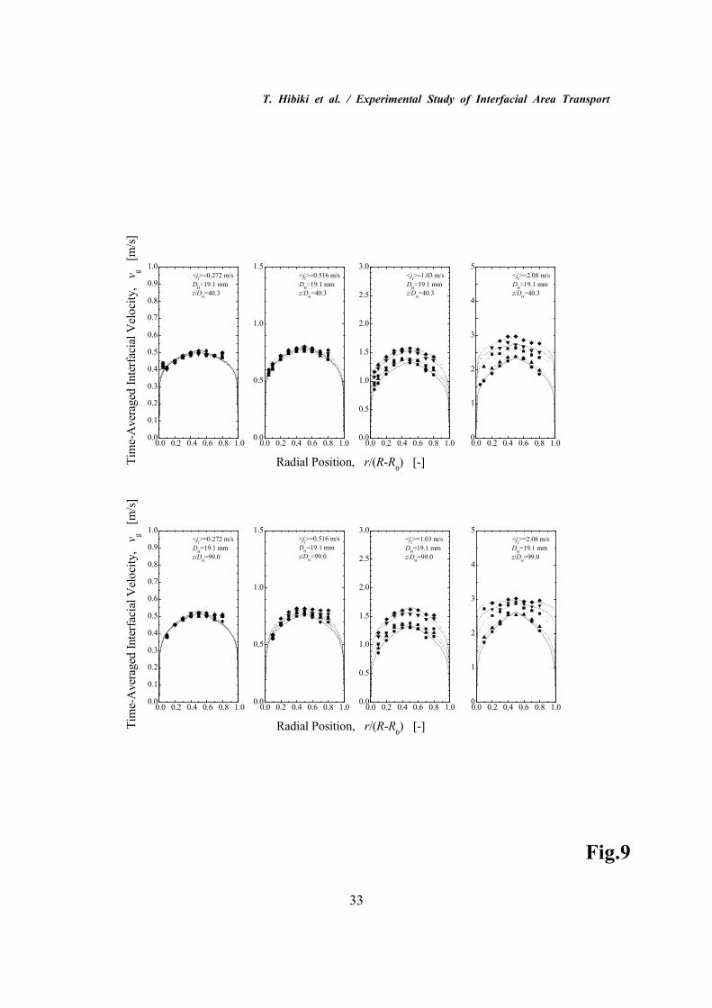
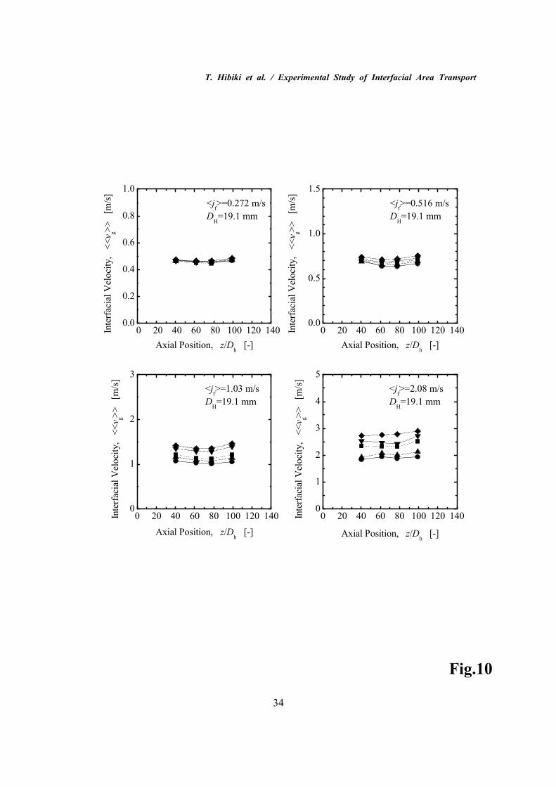
3.1.5. Interfacial velocity

Figure 9 shows the behavior of interfacial velocity profiles, corresponding to that of void

fraction profiles in Fig.2. Figure 10 also shows the axial development of void-fraction-weighted

area-averaged interfacial velocities, <<vg>>, obtained by integrating local interfacial velocity over

the flow channel. The meanings of the symbols in Figs.9 and 11 are found in Table 1. As

expected, the interfacial velocity had a power-law profile. The void-fraction-weighted

area-averaged interfacial velocities were not changed along the flow direction. The local

interfacial velocities can be fitted by the following function.

( )n

ggRR

RRrv

n

nv

1

0

021

1

−

−−−

+= , (1)

where n is the exponent. As shown in Fig.9, measured interfacial velocities could be fitted by

Eq.(1) reasonably well except for <jf>=2.08 m/s and higher void fraction. Figure 11 shows the

dependence of the exponent characterizing the interfacial velocity profile on the void fraction,

<α>, or the superficial liquid velocity, <jf>. As the area-averaged void fraction increased, the

exponent increased gradually, resulting in flatter interfacial velocity profile. As the superficial

liquid velocity increased, the exponent decreased gradually and approached to the asymptotic


16

value. Since the interfacial velocity would have the same tendency of the respective liquid

velocity profile [7], the interfacial velocity profile might be attributed to the balance of the

bubble-induced turbulence and shear-induced turbulence. It was observed in a round tube that

for low liquid superficial velocities (<jf>≤1 m/s) the introduction of bubbles into the liquid flow

flattened the liquid velocity profile and the liquid velocity profile approached to that of developed

single-phase flow with the increase of void fraction [7]. It was also reported that the effect of

the bubble introduction into the liquid on the liquid velocity profile was diminishing with

increasing gas and liquid velocities and for high liquid velocities (<jf>≥1 m/s) the liquid velocity

profile came to be the power law profile as the flow developed. Thus, for low or high liquid

velocity, the bubble-induced or shear-induced turbulence would play an important role in

determining the liquid velocity profile, respectively.

The dependence of the exponent on the void fraction and superficial liquid velocity

might be captured by the following simple correlation.

( ) 0425.0

0

590.0272.0

0 34.2,4341 ff RenRenn ×=+= −α . (2)

In Eq.(2), n0 and Ref are the asymptotic exponent at <α>=0 and the liquid Reynolds number

defined by <jf>DH/νf where νf is the kinetic viscosity of the liquid phase. Since sufficient data

were not available, the asymptotic exponent, n0, was obtained by assuming the same dependence

of the exponent on the liquid Reynolds number as that for a liquid velocity profile in a round tube

and by determining the coefficient from the data obtained by extrapolating the exponent for

<jf>=2.08 m/s at <α>=0. It should be noted here that for <jf>=2.08 m/s the bubble introduction

might not affect the exponent significantly. The lines in Fig.11 indicate the exponent calculated

by Eq.(2), and Eq.(2) reproduced a proper trend of the dependence of the exponent on the flow




17

parameters satisfactorily. The applicability of Eq.(2) to a flow condition over the present flow

conditions should be examined by rigorous data set to be taken in a future study.

3.2 One-dimensional interfacial area transport

In order to develop the area-averaged or one-dimensional interfacial area transport

equation, an accurate data set of the area-averaged flow parameters is indispensable.

Area-averaged interfacial area concentration and Sauter mean diameter are plotted against z/DH in

Figs.8 and 4, respectively. The meanings of the symbols in Figs.8 and 4 are found in Table 1.

Since the bubble expansion due to the pressure reduction can be thought of as the source term of

the interfacial area transport, the axial change of the interfacial area concentration due to the

bubble coalescence and breakup should be extracted from the total axial change of the interfacial

area concentration to understand the mechanism of the interfacial area transport due to the bubble

coalescence and breakup as follows. Ishii et al. [12] derived the one-dimensional interfacial area

transport equation for bubbly flow taking the gas expansion along the flow direction into account

as:

( )

( ) ,3

2

3

12

+

+

+

=

+

∑ g

i

ph

j

j

i

agi

i

vdz

d

t

aSS

a

vadz

d

t

a

α∂α∂

αα

ψ

∂∂

(3)

where ψ is the factor depending on the shape of a bubble (1/36π for a spherical bubble), and Sj,

and Sph denote the sink or source terms in the interfacial area concentration due to bubble

coalescence or breakup, and the sink or source terms in the interfacial area concentration due to

phase change, respectively. The brackets of << >>a and << >> mean the interfacial area


18

concentration weighted cross-sectional area-averaged quantity, and the void fraction weighted

cross-sectional area-averaged quantity, respectively. Equation (3) can be simplified as follows

on the assumptions of (i) no phase change (<Sph>=0), (ii) steady flow (∂<ai>/∂t=0, ∂<α>/∂t=0),

(iii) equilibrium of bubble coalescence and breakup rates ( 0=∑j

jS ),and (iv) <<vg>>a=<<vg>>.

The assumption (iv) would be sound for almost spherical bubbles.

0,

3/2

0

, ieqi aP

Pa

= , (4)

where ai,eq, ai,0, P, and P0 denote the local interfacial area concentration under the conditions of

no phase change and equilibrium of bubble coalescence and breakup rates, the inlet interfacial

area concentration, the local pressure, and the inlet pressure, respectively. The ratio of

area-averaged interfacial area concentration, <ai>, to <ai,eq>., ξ(≡<ai>/<ai,eq.>) represents the net

change in the interfacial area concentration due to the bubble coalescence and breakup. ξ>1 or

ξ<1 implies that the bubble breakup or coalescence is dominant, respectively. It should be noted

here that ξ becomes identical to a bubble number density ratio, if further assumptions such as (v)

a spherical bubble and (vi) a uniform bubble distribution are made.

eqi

i

eqi

i

i

i

a

a

P

P

P

P

a

a

a

a

,

3/2

0

3/2

0

,0,

, ≡

=

= ξξ . (5)

In a forced convective pipe flow or mechanically agitated systems, the initial bubble size

may be too large or too small to be stable. In these cases, the bubble size is further determined

by a coalescence and/or breakup mechanism. The changes in the interfacial area concentration

due to the bubble coalescence and breakup, ξ, between z/DH=40.3 and 99.9 are plotted against the


19

void fraction, <α>, or the superficial liquid velocity, <jf> in Fig.12. The meanings of the

symbols in Fig.12 are found in Table 1. It should be noted in Fig.12 that the interfacial area

concentration and the pressure at z/DH=40.3 was taken as <ai,0> and P0, respectively, and

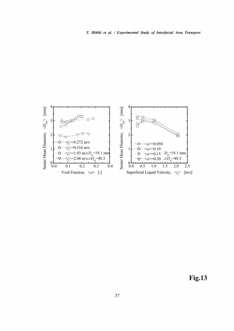
measured P were used in the calculation of ξ. Figure 13 shows the dependence of the Sauter

mean diameter, <DSm>, measured at z/DH=40.3 on the void fraction, <α>, or the superficial liquid

velocity, <jf>. It can be found that in this experiment bubbles with the diameters of about 3 mm

and 2 mm were generated at z/DH=40.3 for <jf>≤1 m/s and <jf>=2 m/s, respectively. For

<jf>=0.272 m/s and <α>≤0.10, the bubble size at z/DH=40.3, which was formed in this

experiment, would be smaller to be stable for the flow condition. In this case, the dominant

mechanism on the interfacial area transport would be the bubble coalescence due to collision

between bubbles induced by liquid turbulence. For <jf>=0.516 and 1.03 m/s and <α>=0.05, the

bubble size at z/DH=40.3, which was formed in this experiment, would be larger to be stable for

the flow conditions. In this case, the dominant mechanism on the interfacial area transport

would be the bubble breakup due to collision between a bubble and a turbulence eddy. For

<jf>≤1.0 m/s and 0.1≤<α>≤0.2, the bubble size at z/DH=40.3 would be stable. In this case,

insignificant interfacial area transport between z/DH=40.3 and 99.9, namely, ξ≈1, was observed.

For <jf>=2.08 m/s, the bubble size at z/DH=40.3, which was formed in this experiment, would be

smaller to be stable for the flow condition. In this case, a strong liquid turbulence might

promote the bubble coalescence rather than the bubble breakup. Thus, the bubble size as well as

the void fraction and liquid turbulence would be a key factor to determine the dominant factor of

the interfacial area transport [2].

The data from the double-sensor conductivity probe give near complete information on

the time-averaged local hydrodynamic parameters of bubbly flow to model and evaluate the sink



20

and source terms of interfacial area concentration. For example, some attempts have been

performed to model the sink and source terms in a round tube based on mechanisms of bubble

coalescence due to bubble random collision and bubble breakup due to bubble-turbulent eddy

random collision, respectively [2, 12, 13]. As a first step, the applicability of the modeled

interfacial area transport equation in a round tube to a flow in an annulus will be tested by using

the data taken in this study. Thus, the data set obtained in this study will eventually be used for

the development of reliable constitutive relations, which reflect the true transfer mechanisms in

bubbly flow systems.

4. Conclusions

As a first step of the development of the interfacial area transport equation in a

subcooled boiling flow, hydrodynamic separate tests without phase change were performed to

identify the effect of bubble coalescence and breakup on the interfacial area transport. Axial

developments of local void fraction, interfacial area concentration, and interfacial velocity of

vertical upward air-water bubbly flows in an annulus were measured by using the double-sensor

conductivity probe method. The annulus channel consisted of an inner rod with a diameter of

19.1 mm and an outer round tube with an inner diameter of 38.1 mm, and the hydraulic

equivalent diameter was 19.1 mm. A total of 20 data sets were acquired consisting of five void

fractions, about 0.050, 0.10, 0.15, 0.20, and 0.25, and four superficial liquid velocities, 0.272,

0.516, 1.03, and 2.08 m/s. The measurements for each flow condition were performed at four

axial locations: axial locations non-dimensionalized by the hydraulic equivalent diameter = 40.3,

61.7, 77.7, and 99.0. The mechanisms to form the radial profiles of local flow parameters and

their axial developments were discussed in detail. The one-dimensional interfacial area


https://www.researchgate.net/publication/222615321_One-group_interfacial_area_transport_in_vertical_bubbly_flow?el=1_x_8&enrichId=rgreq-58170fa3de37652cf17a03628cbe0f53-XXX&enrichSource=Y292ZXJQYWdlOzIyMjA2MzE2MjtBUzoxNTI5NzYzNTQxODkzMTVAMTQxMzQ4MzgxMzgxMw==


21

transport due to the bubble coalescence and breakup was displayed against the void fraction and

superficial liquid velocity. The bubble size as well as the void fraction and liquid turbulence

was likely to be a key factor to determine the dominant factor of the interfacial area transport.

The data set obtained in this study are expected to be used for the development of

reliable constitutive relations such as the interfacial area transport equation, which reflect the true

transfer mechanisms in subcooled boiling flow systems.

Acknowledgments

The research project was supported by the Tokyo Electric Power Company (TEPCO).

The authors would like to express their sincere appreciation for the support and guidance from Dr.

Mori of the TEPCO.

References

[1] G. Kocamustafaogullari, M. Ishii, Foundation of the interfacial area transport equation and

its closure relations, International Journal of Heat and Mass Transfer 38 (1995) 481-493.

[2] T. Hibiki, M. Ishii, Development of one-group interfacial area transport equation in bubbly

flow systems, International Journal of Heat and Mass Transfer 45 (2002) 2351-2372.

[3] M. D. Bartel, M. Ishii, T. Masukawa, Y. Mi, R. Situ, Interfacial area measurements in

subcooled flow boiling, Nuclear Engineering and Design 210 (2001) 135-155.

[4] S. Kim, X. Y. Fu, X. Wang, M. Ishii, Development of the miniaturized four-sensor

conductivity probe and the signal processing scheme, International Journal of Heat and

Mass Transfer 43 (2000) 4101-4118.

[5] T. Hibiki, Y. Mi, R. Situ, M. Ishii, M. Mori, Interfacial area transport of vertical upward








22

bubbly flow in an annulus, Proceedings of International Congress on Advanced Nuclear

Power Plants, Hollywood, Florida, USA (2002).

[6] T. Hibiki, M. Ishii, Experimental study on interfacial area transport in bubbly two-phase

flows, International Journal of Heat and Mass Transfer 42 (1999) 3019-3035.

[7] T. Hibiki, M. Ishii, Z. Xiao, Axial interfacial area transport of vertical bubbly flows,

International Journal of Heat and Mass Transfer 44 (2001) 1869-1888.

[8] A. Serizawa, I. Kataoka, Phase distribution in two-phase flow, in : N. H. Afgan (Ed.),

Transient Phenomena in Multiphase Flow, Hemisphere, Washington, DC, 1988,

pp.179-224.

[9] K. Sekoguchi, T. Sato, T. Honda, Two-phase bubbly flow (first report), Transactions of

JSME 40 (1974) 1395-1403 (in Japanese).

[10] I. Zun, Transition from wall void peaking to core void peaking in turbulent bubbly flow, in :

N. H. Afgan (Ed.), Transient Phenomena in Multiphase Flow, Hemisphere, Washington,

DC, 1988, pp.225-245.

[11] Y. Taitel, D. Bornea, E. A. Dukler, Modelling flow pattern transitions for steady upward

gas-liquid flow in vertical tubes, AIChE Journal 26 (1980) 345-354.

[12] M. Ishii, Q. Wu, S. T. Revankar, T. Hibiki, W. H. Leung, S. Hogsett, A. Kashyap,

Interfacial area transport in bubbly flow, in: Proceedings of 15th Symposium on Energy

Engineering Science, Argonne, IL, USA, 1997.

[13] Q. Wu, S. Kim, M. Ishii, S. G. Beus, One-group interfacial area transport in vertical bubbly

flow, International Journal of Heat and Mass Transfer 41 (1998) 1103-1112.










23

Table 1 Flow conditions in this experiment.

Symbols ● ▲ ■ ▼ ◆

<jf>

[m/s]

<jg,N>

[m/s]

<jg, N>

[m/s]

<jg, N >

[m/s]

<jg, N>

[m/s]

<jg, N>

[m/s]

0.272 0.0313 0.0506 0.0690 0.0888 0.105

0.516 0.0406 0.0687 0.103 0.135 0.176

1.03 0.0683 0.130 0.201 0.400 0.489

2.08 0.108 0.215 0.505 0.651 0.910

Figure Captions

Fig.1 Schematic diagram of experimental loop.

Fig.2. Local void fraction profiles at z/DH=40.3 and 99.9.

Fig.3. Dependence of peak void fraction and radial position on void fraction and superficial

liquid velocity.

Fig.4. Axial development of area-averaged Sauter mean diameter.

Fig.5. Map of phase distribution patterns.

Fig.6. Local Sauter mean diameter profiles at z/DH=40.3 and 99.9.

Fig.7. Local interfacial area concentration profiles at z/DH=40.3 and 99.9.

Fig.8. Axial development of area-averaged interfacial area concentration.

Fig.9. Local interfacial velocity profiles at z/DH=40.3 and 99.9.

Fig.10. Axial development of void-fraction-weighted mean interfacial velocity.

Fig.11. Dependence of interfacial velocity profile on void fraction and superficial liquid


24

velocity.

Fig.12. Dependence of interfacial area transport due to bubble coalescence and breakup on

void fraction and superficial liquid velocity.

Fig.13 Dependence of bubble size on void fraction and superficial liquid velocity.


25

HeaterCooler

Flexible

Pipe

Separation

Tank

MainTank

Flowmeter PumpHeater

Rod

Height

Adjuster

Test

Section

Air Supply

T.C.

Filter

Drain

Degasing

Cooler

Drain

Drain

T.C.

T.C. T.C.

Condensation

TankD.P.

Air Flowmeters

P

P

Fig.1


26

Fig.2

0.0 0.2 0.4 0.6 0.8 1.00.0

0.1

0.2

0.3

0.4

0.5

0.6

<jf>=0.272 m/s

DH=19.1 mm

z/DH=40.3

Tim

e-Averaged Void Fraction, α [-]

0.0 0.2 0.4 0.6 0.8 1.00.0

0.1

0.2

0.3

0.4

0.5

0.6

<jf>=0.516 m/s

DH=19.1 mm

z/DH=40.3

0.0 0.2 0.4 0.6 0.8 1.00.0

0.1

0.2

0.3

0.4

0.5

0.6

<jf>=1.03 m/s

DH=19.1 mm

z/DH=40.3

Radial Position, r/(R-R0) [-]

0.0 0.2 0.4 0.6 0.8 1.00.0

0.1

0.2

0.3

0.4

0.5

0.6

<jf>=2.08 m/s

DH=19.1 mm

z/DH=40.3

0.0 0.2 0.4 0.6 0.8 1.00.0

0.1

0.2

0.3

0.4

0.5

0.6

<jf>=0.272 m/s

DH=19.1 mm

z/DH=99.0

Tim

e-Averaged Void Fraction, α [-]

0.0 0.2 0.4 0.6 0.8 1.00.0

0.1

0.2

0.3

0.4

0.5

0.6

<jf>=0.516 m/s

DH=19.1 mm

z/DH=99.0

0.0 0.2 0.4 0.6 0.8 1.00.0

0.1

0.2

0.3

0.4

0.5

0.6

<jf>=1.03 m/s

DH=19.1 mm

z/DH=99.0


0.0 0.2 0.4 0.6 0.8 1.00.0

0.1

0.2

0.3

0.4

0.5

0.6

<jf>=2.08 m/s

DH=19.1 mm

z/DH=99.0


27

Fig.3

0.0 0.1 0.2 0.3 0.4 0.50.0

0.2

0.4

0.6

0.8

1.0

Inner Side

DH=19.1 mm

z/DH=99.0

<jf>=0.272 m/s

<jf>=0.516 m/s

<jf>=1.03 m/s

<jf>=2.08 m/s

Non-D

Peak Void Fraction, (α

P-α

C)/αP [-]

Void Fraction, <α> [-]

0.0 0.1 0.2 0.3 0.4 0.50.0

0.2

0.4

0.6

0.8

1.0

Outer Side

DH=19.1 mm

z/DH=99.0

Outer Side

DH=19.1 mm

z/DH=99.0

<jf>=0.272 m/s

<jf>=0.516 m/s

<jf>=1.03 m/s

<jf>=2.08 m/s

Non-D

Peak Void Fraction, (α

P-α

C)/αP [-]


0.0 0.1 0.2 0.3 0.4 0.50.0

0.1

0.2

0.3

0.4

0.5

Inner Side

DH=19.1 mm

z/DH=99.0

<jf>=0.272 m/s

<jf>=0.516 m/s

<jf>=1.03 m/s

<jf>=2.08 m/s

Non-D

Peak Position, r P/(

R-R

0) [-]


0.0 0.1 0.2 0.3 0.4 0.50.0

0.1

0.2

0.3

0.4

0.5

<jf>=0.272 m/s

<jf>=0.516 m/s

<jf>=1.03 m/s

<jf>=2.08 m/s

Non-D

Peak Position, 1-r

P/(

R-R

0) [-]



28

Fig.4

0 20 40 60 80 100 120 1402

3

4

5

<jf>=0.272 m/s

DH=19.1 mm

Sauter Mean Dia., <

DSm> [mm]

Axial Position, z/Dh [-]

0 20 40 60 80 100 120 1402

3

4

5

<jf>=0.516 m/s

DH=19.1 mm

Sauter Mean Dia., <

DSm> [mm]


0 20 40 60 80 100 120 1402

3

4

5

<jf>=1.03 m/s

DH=19.1 mm

Sauter Mean Dia., <

DSm> [mm]


0 20 40 60 80 100 120 1401

2

3

4

5

<jf>=2.08 m/s

DH=19.1 mm

Sauter Mean Dia., <

DSm> [mm]



29

Fig.5

10-2

10-1

100

101

10-1

100

101

Core Peak

Intermediate Peak

Wall Peak

Transition

Slug Flow

Bubbly Flow

Finely Dispersed Bubbly Flow

DH=19.1 mm

z/DH=99.0

Transition

Core

Serizawa & Kataoka

Wall

Intermediate

Taitel et al.

Superficial Liquid Velocity, <j f> [m/s]

Superficial Gas Velocity, <jg> [m/s]


30

Fig.6

0.0 0.2 0.4 0.6 0.8 1.00

1

2

3

4

5

6

7

<jf>=0.272 m/s

DH=19.1 mm

z/DH=40.3

Tim

e-Averaged Sauter Mean Dia., D

Sm [mm]

0.0 0.2 0.4 0.6 0.8 1.00

1

2

3

4

5

6

7

<jf>=0.516 m/s

DH=19.1 mm

z/DH=40.3

0.0 0.2 0.4 0.6 0.8 1.00

1

2

3

4

5

6

7

<jf>=1.03 m/s

DH=19.1 mm

z/DH=40.3


0.0 0.2 0.4 0.6 0.8 1.00

1

2

3

4

5

6

7

<jf>=2.08 m/s

DH=19.1 mm

z/DH=40.3

0.0 0.2 0.4 0.6 0.8 1.00

1

2

3

4

5

6

7

<jf>=0.272 m/s

DH=19.1 mm

z/DH=99.0

Tim

e-Averaged Sauter Mean Dia., D

Sm [mm]

0.0 0.2 0.4 0.6 0.8 1.00

1

2

3

4

5

6

7

<jf>=0.516 m/s

DH=19.1 mm

z/DH=99.0

0.0 0.2 0.4 0.6 0.8 1.00

1

2

3

4

5

6

7

<jf>=1.03 m/s

DH=19.1 mm

z/DH=99.0


0.0 0.2 0.4 0.6 0.8 1.00

1

2

3

4

5

6

7

<jf>=2.08 m/s

DH=19.1 mm

z/DH=99.0


31

Fig.7

0.0 0.2 0.4 0.6 0.8 1.00

500

1000

1500

<jf>=0.272 m/s

DH=19.1 mm

z/DH=40.3

Tim

e-Averaged IAC, ai [m

-1]

0.0 0.2 0.4 0.6 0.8 1.00

500

1000

1500

<jf>=0.516 m/s

DH=19.1 mm

z/DH=40.3

0.0 0.2 0.4 0.6 0.8 1.00

500

1000

1500

<jf>=1.03 m/s

DH=19.1 mm

z/DH=40.3


0.0 0.2 0.4 0.6 0.8 1.00

500

1000

1500

<jf>=2.08 m/s

DH=19.1 mm

z/DH=40.3

0.0 0.2 0.4 0.6 0.8 1.00

500

1000

1500

<jf>=0.272 m/s

DH=19.1 mm

z/DH=99.0

Tim

e-Averaged IAC, ai [m

-1]

0.0 0.2 0.4 0.6 0.8 1.00

500

1000

1500

<jf>=0.516 m/s

DH=19.1 mm

z/DH=99.0

0.0 0.2 0.4 0.6 0.8 1.00

500

1000

1500

<jf>=1.03 m/s

DH=19.1 mm

z/DH=99.0


0.0 0.2 0.4 0.6 0.8 1.00

500

1000

1500

<jf>=2.08 m/s

DH=19.1 mm

z/DH=99.0


32

Fig.8

0 20 40 60 80 100 120 1400

200

400

600

800

<jf>=0.272 m/s

DH=19.1 mm

Interfacial Area Conc., <ai> [m

-1]


0 20 40 60 80 100 120 1400

200

400

600

800

<jf>=0.516 m/s

DH=19.1 mm


-1]


0 20 40 60 80 100 120 1400

200

400

600

800

1000

1200

<jf>=1.03 m/s

DH=19.1 mm


-1]


0 20 40 60 80 100 120 1400

200

400

600

800

1000

1200

<jf>=2.08 m/s

DH=19.1 mm


-1]



33

Fig.9

0.0 0.2 0.4 0.6 0.8 1.00.0

0.1

0.2

0.3

0.4

0.5

0.6

0.7

0.8

0.9

1.0

<jf>=0.272 m/s

DH=19.1 mm

z/DH=40.3

Tim

e-Averaged Interfacial Velocity, v g [m/s]

0.0 0.2 0.4 0.6 0.8 1.00.0

0.5

1.0

1.5

<jf>=0.516 m/s

DH=19.1 mm

z/DH=40.3

0.0 0.2 0.4 0.6 0.8 1.00.0

0.5

1.0

1.5

2.0

2.5

3.0

<jf>=1.03 m/s

DH=19.1 mm

z/DH=40.3


0.0 0.2 0.4 0.6 0.8 1.00

1

2

3

4

5

<jf>=2.08 m/s

DH=19.1 mm

z/DH=40.3

0.0 0.2 0.4 0.6 0.8 1.00.0

0.1

0.2

0.3

0.4

0.5

0.6

0.7

0.8

0.9

1.0

<jf>=0.272 m/s

DH=19.1 mm

z/DH=99.0

Tim

e-Averaged Interfacial Velocity, v g [m/s]

0.0 0.2 0.4 0.6 0.8 1.00.0

0.5

1.0

1.5

<jf>=0.516 m/s

DH=19.1 mm

z/DH=99.0

0.0 0.2 0.4 0.6 0.8 1.00.0

0.5

1.0

1.5

2.0

2.5

3.0

<jf>=1.03 m/s

DH=19.1 mm

z/DH=99.0


0.0 0.2 0.4 0.6 0.8 1.00

1

2

3

4

5

<jf>=2.08 m/s

DH=19.1 mm

z/DH=99.0


34

Fig.10

0 20 40 60 80 100 120 1400.0

0.2

0.4

0.6

0.8

1.0

<jf>=0.272 m/s

DH=19.1 mm

Interfacial Velocity, <<v g>> [m/s]


0 20 40 60 80 100 120 1400.0

0.5

1.0

1.5

<jf>=0.516 m/s

DH=19.1 mm



0 20 40 60 80 100 120 1400

1

2

3

<jf>=1.03 m/s

DH=19.1 mm



0 20 40 60 80 100 120 1400

1

2

3

4

5

<jf>=2.08 m/s

DH=19.1 mm




35

Fig.11

0.0 0.1 0.2 0.3 0.40

5

10

15

DH=19.1 mm

<jf>=0.272 m/s

<jf>=0.516 m/s

<jf>=1.03 m/s

<jf>=2.08 m/s

Exponent, n [-]


0.0 0.5 1.0 1.5 2.0 2.50

5

10

15

DH=19.1 mm

<α>=0.050 <α>=0.10 <α>=0.15

Exponent, n [-]

Superficial Liquid Velocity, <jf> [m/s]


36

Fig.12

0.0 0.1 0.2 0.3 0.40.0

0.5

1.0

1.5

Breakup

Coalescence

DH=19.1 mm

z/DH=99.0

<jf>=0.272 m/s

<jf>=0.516 m/s

<jf>=1.03 m/s

<jf>=2.08 m/s

IAC Change Due to Bubble Coalescence &

Breakup, ξ [-]


0.0 0.5 1.0 1.5 2.0 2.50.0

0.5

1.0

1.5

Breakup

Coalescence

DH=19.1 mm

z/DH=99.0

<α>=0.050 <α>=0.10 <α>=0.15 <α>=0.20

IAC Change Due to Bubble Coalescence &

Breakup, ξ [-]



37

Fig.13

0.0 0.1 0.2 0.3 0.40

1

2

3

4

DH=19.1 mm

z/DH=40.3

<jf>=0.272 m/s

<jf>=0.516 m/s

<jf>=1.03 m/s

<jf>=2.08 m/s

Sauter Mean Diameter, <D

Sm> [mm]


0.0 0.5 1.0 1.5 2.0 2.50

1

2

3

4

DH=19.1 mm

z/DH=40.3

<α>=0.050 <α>=0.10 <α>=0.15 <α>=0.20

Sauter Mean Diameter, <D

Sm> [mm]


experimental study on interfacial area transport in bubbly two-phase flows

Documents