kncourse2: clustering and blockmodeling / 2. approaches to clustering

'&

$%

Methods of Network Analysis

Clustering and Blockmodeling2. Approaches to Clustering

Vladimir BatageljUniversity of Ljubljana, Slovenia

University of Konstanz, Algorithms and Data Structures

June 6, 2002, 14-16h, room F 426

V. Batagelj: Clustering and Blockmodeling 0/2'

&

$%

Approaches to Clustering

� local optimization

� dynamic programming

� hierarchical methods; agglomerative methods; Lance-Williams formula;

dendrogram; inversions; adding methods

� leaders and the dynamic clusters method

� graph theory (next, 3. lecture);

University of Konstanz June 2002


&

$%

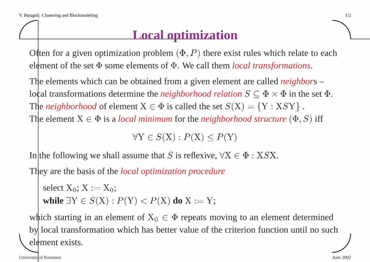
Local optimizationOften for a given optimization problem(�; P ) there exist rules which relate to eachelement of the set� some elements of�. We call themlocal transformations.

The elements which can be obtained from a given element are called neighbors –local transformations determine theneighborhood relationS � �� in the set�.Theneighborhoodof elementX 2 � is called the setS(X) = fY : XSYg .The elementX 2 � is a local minimumfor theneighborhood structure(�; S) iff

8Y 2 S(X) : P (X) � P (Y)

In the following we shall assume thatS is reflexive,8X 2 � : XSX.

They are the basis of thelocal optimization procedure

selectX0

; X := X

0

;

while 9Y 2 S(X) : P (Y) < P (X) doX := Y;

which starting in an element ofX0

2 � repeats moving to an element determinedby local transformation which has better value of the criterion function until no suchelement exists.



&

$%

Clustering neigborhoods

Usually the neighborhood relation in local optimization clustering procedures over

P

k

(U) is determined by the following two transformations:

� transition: clusteringC0 is obtained fromC by moving a unit from one cluster to

another

C

0

= (C n fC

u

; C

v

g) [ fC

u

n fX

s

g; C

v

[ fX

s

gg

� transposition: clusteringC0 is obtained fromC by interchanging two units from

different clusters

C

0

= (C n fC

u

; C

v

g) [ f(C

u

n fX

p

g) [ fX

q

g; (C

v

n fX

q

g) [ fX

p

gg

The transpositions preserve the number of units in clusters.



&

$%

Hints

Two basic implementation approaches are usually used:stored dataapproach and

stored dissimilarity matrixapproach.

If the constraints are not too stringent, the relocation method can be applied directly

on�; otherwise, we can transform usingpenalty function methodthe problem to an

equivalent nonconstrained problem(Pk

; Q) with Q(C) = P (C) + �K(C) where

� > 0 is a large constant andK(C) = 0, forC 2 �, andK(C) > 0 otherwise.

There exist several improvements of the basic relocation algorithm: simulated

annealing, tabu search, . . . (Aarts and Lenstra, 1997).

The initial clusteringC0

can be given; most often we generate it randomly.

Let [s℄ = u , X

s

2 C

u

. Fill the vector with the desired number of units in each

cluster and shuffle it:

for p := n downto 2 do beginq := random(1; p); swap( [p℄; [q℄) end;



&

$%

Quick scanning of neighbors

TestingP (C0

) < P (C) is equivalent toP (C)� P (C

0

) > 0.

For theS criterion function

�P (C;C

0

) = P (C)� P (C

0

) = p(C

u

) + p(C

v

)� p(C

0

u

)� p(C

0

v

)

Additional simplifications can be done considering relations betweenCu

andC0

u

, and

betweenCv

andC0

v

.

Let us illustrate this on the generalized Ward’s method. Forthis purpose it is useful to introduce

the quantity

a(C

u

; C

v

) =

X

X2C

u

;Y2C

v

w(X) � w(Y) � d(X;Y)

Using the quantitya(Cu

; C

v

) we can expressp(C) in the formp(C) =

a(C;C)

2w(C)

and the equality

mentioned in the introduction of the generalized Ward clustering problem: ifCu

\C

v

= ; then

w(C

u

[ C

v

) � p(C

u

[ C

v

) = w(C

u

) � p(C

u

) + w(C

v

) � p(C

v

) + a(C

u

; C

v

)



&

$%

� for the generalized Ward’s method

Let us analyze the transition of a unitXs

from clusterCu

to clusterCv

:

We haveC0

u

= C

u

n fX

s

g , C0

v

= C

v

[ fX

s

g ,

w(C

u

) � p(C

u

) = w(C

0

u

) � p(C

0

u

) + a(X

s

; C

0

u

) = (w(C

u

)� w(X

s

)) � p(C

0

u

) + a(X

s

; C

0

u

)

andw(C

0

v

) � p(C

0

v

) = w(C

v

) � p(C

v

) + a(X

s

; C

v

)

Fromd(X

s

;X

s

) = 0 it follows a(Xs

; C

u

) = a(X

s

; C

0

u

). Therefore

p(C

0

u

) =

w(C

u

) � p(C

u

)� a(X

s

; C

u

)

w(C

u

)� w(X

s

)

p(C

0

v

) =

w(C

v

) � p(C

v

) + a(X

s

; C

v

)

w(C

v

) + w(X

s

)

and finally

�P (C;C

0

) = p(C

u

) + p(C

v

)� p(C

0

u

)� p(C

0

v

) =

=

w(X

s

) � p(C

v

)� a(X

s

; C

v

)

w(C

v

) + w(X

s

)

�

w(X

s

) � p(C

u

)� a(X

s

; C

u

)

w(C

u

)� w(X

s

)

In the case whend is the squared Euclidean distance it is possible to derive also expression for

corrections of centers (Spath, 1977).



&

$%

Dynamic programmingSuppose thatMin(�

k

; P ) 6= ;, k = 1; 2; : : :. DenotingP �

(U; k) = P (C�k

(U)) we

can derive the generalizedJensen equality(Batagelj, Korenjak and Klavzar, 1994):

P

�

(U; k) =

8><

>:

p(U) fUg 2 �

1

min

;�C�U

9C2�

k�1

(UnC):C[fCg2�

k

(U)

(P

�

(U n C; k � 1)� p(C)) k > 1

This is adynamic programming(Bellman) equation which, for some special con-

strained problems, that keep the size of�k

small, allows us to solve the clustering

problem by the adapted Fisher’s algorithm.



&

$%

Hierarchical methodsThe set of feasible clusterings� determines thefeasibility predicate�(C) � C 2 �

defined onP(P(U) n f;g); and conversely� � fC 2 P(P(U) n f;g) : �(C)g.

In the set� the relation ofclustering inclusionv can be introduced byC

1

v C

2

� 8C

1

2 C

1

; C

2

2 C

2

: C

1

\ C

2

2 f;; C

1

g

we say also that the clusteringC1

is arefinementof the clusteringC2

.

It is well known that(P (U);v) is a partially ordered set (even more, semimodular

lattice). Because any subset of partially ordered set is also partially ordered, we have:

Let� � P (U) then(�;v) is a partially ordered set.

The clustering inclusion determines two related relations(on�):

C

1

< C

2

� C

1

v C

2

^C

1

6= C

2

– strict inclusion, and

C

1

<� C

2

� C

1

< C

2

^ :9C 2 � : (C

1

< C ^C < C

2

) – predecessor.



&

$%

Conditions on the structure of the set of feasible clusterings

We shall assume that the set of feasible clusterings� � P (U) satisfies the following

conditions:

F1. O � ffXg : X 2 Ug 2 �

F2. The feasibility predicate� is local – it has the form�(C) =V

C2C

'(C)

where'(C) is a predicate defined onP(U) n f;g (clusters).

The intuitive meaning of'(C) is: '(C) � the clusterC is ’good’. Therefore the

locality condition can be read: a ’good’ clusteringC 2 � consists of ’good’ clusters.

F3. The predicate� has the property ofbinary hereditywith respect to thefusibility

predicate (C1

; C

2

), i.e.,

C

1

\ C

2

= ; ^ '(C

1

) ^ '(C

2

) ^ (C

1

; C

2

)) '(C

1

[ C

2

)

This condition means: in a ’good’ clustering, a fusion of two’fusible’ clusters

produces a ’good’ clustering.



&

$%

. . . conditions

F4. The predicate is compatiblewith clustering inclusionv, i.e.,

8C

1

;C

2

2 � : (C

1

< C

2

^C

1

nC

2

= fC

1

; C

2

g ) (C

1

; C

2

) _ (C

2

; C

1

))

F5. The interpolationproperty holds in�, i.e., 8C

1

;C

2

2 � :

(C

1

< C

2

^ ard(C

1

) > ard(C

2

) + 1) 9C 2 � : (C

1

< C ^C < C

2

))

These conditions provide a framework in which the hierarchical methods can be

applied also for constrained clustering problems�k

(U) � P

k

(U).

In the ordinary problem both predicates'(C) and (Cp

; C

q

) are always true – all

conditions F1-F5 are satisfied.



&

$%

Criterion functions compatible with a dissimilarity between clusters

We shall call adissimilarity between clustersa functionD : (C

1

; C

2

)! IR+0

which is

symmetric, i.e.,D(C1

; C

2

) = D(C

2

; C

1

).

Let (IR+0

;�; 0;�) be an ordered abelian monoid. Then the criterion function

P (C) =

L

C2C

p(C), 8X 2 U : p(fXg) = 0 is compatiblewith dissimilarityD

over� iff for all C � U holds:

'(C) ^ ard(C) > 1) p(C) = min

(C

1

;C

2

)2(C)

(p(C

1

)� p(C

2

)�D(C

1

; C

2

))

Theorem 2.1 A S criterion function is compatible with dissimilarityD defined by

D(C

p

; C

q

) = p(C

p

[ C

q

)� p(C

p

)� p(C

q

)

In this case, letC0

= C n fC

p

; C

q

g [ fC

p

[ C

q

g, Cp

; C

q

2 C, then

P (C

0

)� P (C) = D(C

p

; C

q

)



&

$%

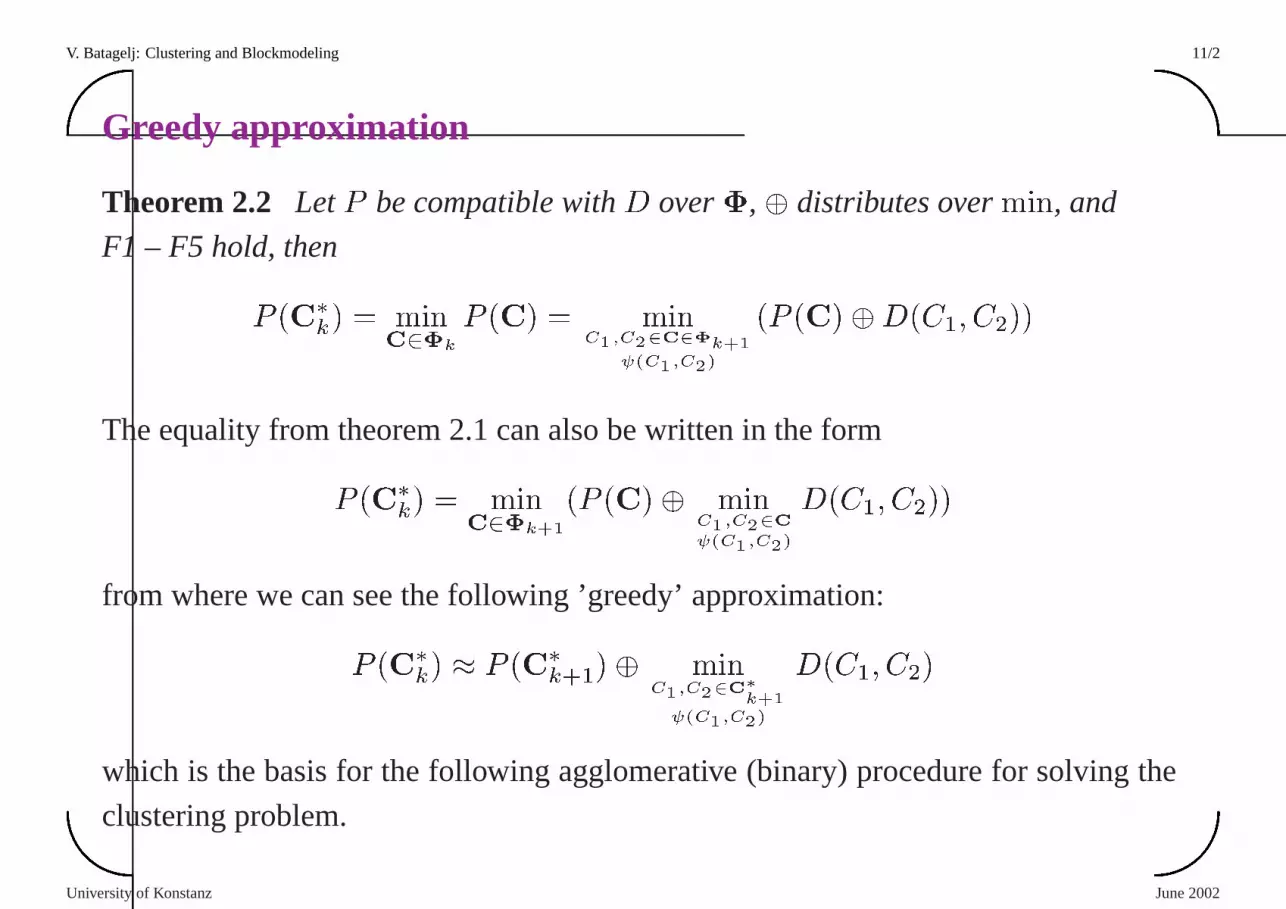
Greedy approximation

Theorem 2.2 LetP be compatible withD over�,� distributes overmin, and

F1 – F5 hold, thenP (C

�k

) = min

C2�

k

P (C) = min

C

1

;C

2

2C2�

k+1

(C

1

;C

2

)

(P (C)�D(C

1

; C

2

))

The equality from theorem 2.1 can also be written in the form

P (C

�k

) = min

C2�

k+1

(P (C)� min

C

1

;C

2

2C

(C

1

;C

2

)

D(C

1

; C

2

))

from where we can see the following ’greedy’ approximation:

P (C

�k

) � P (C

�k+1

)� min

C

1

;C

2

2C

�k+1

(C

1

;C

2

)

D(C

1

; C

2

)

which is the basis for the following agglomerative (binary)procedure for solving the

clustering problem.



&

$%

Agglomerative methods

1. k := n; C(k) := ffXg : X 2 Ug;

2. while 9Ci

; C

j

2 C(k): (i 6= j ^ (C

i

; C

j

)) repeat2.1. (C

p

; C

q

) := argminfD(C

i

; C

j

): i 6= j ^ (C

i

; C

j

)g;

2.2. C := C

p

[ C

q

; k := k � 1;

2.3. C(k) := C(k + 1) n fC

p

; C

q

g [ fCg;

2.4. determineD(C;Cs

) for all Cs

2 C(k)

3. m := k

Note that, because it is based on an approximation, this procedure is not an exact

procedure for solving the clustering problem.

For another,probabilistic view on agglomerative methods see Kamvar, Klein,

Manning (2002).

Divisivemethods work in the reverse direction. The problem here is how to efficiently

find a good split(Cp

; C

q

) of clusterC.



&

$%

Some dissimilarities between clusters

We shall use the generalized Ward’s c.e.f.

p(C) =

1

2w(C)

X

X;Y 2C

w(X) � w(Y ) � d(X;Y )

and the notion of thegeneralized centerC of the clusterC, for which the dissimilarity

to any cluster or unit U is defined by

d(U;C) = d(C;U) =

1

w(C)

(

X

X2C

w(X) � d(X;U)� p(C))

Minimal: Dm

(C

u

; C

v

) = min

X2C

u

;Y 2C

v

d(X;Y )

Maximal:DM

(C

u

; C

v

) = max

X2C

u

;Y 2C

v

d(X;Y )

Average:Da

(C

u

; C

v

) =

1

w(C

u

)w(C

v

)

X

X2C

u

;Y 2C

v

w(X) � w(Y ) � d(X;Y )



&

$%

. . . some dissimilarities

Gower-Bock:DG

(C

u

; C

v

) = d(C

u

; C

v

) = D

a

(C

u

; C

v

)�

p(C

u

)

w(C

u

)

�

p(C

v

)

w(C

v

)

Ward:DW

(C

u

; C

v

) =

w(C

u

)w(C

v

)

w(C

u

[ C

v

)

D

G

(C

u

; C

v

)

Inertia:DI

(C

u

; C

v

) = p(C

u

[ C

v

)

Variance:DV

(C

u

; C

v

) = var(C

u

[ C

v

) =

p(C

u

[ C

v

)

w(C

u

[ C

v

)

Weighted increase of variance:

D

v

(C

u

; C

v

) = var(C

u

[C

v

)�

w(C

u

) � var(C

u

) + w(C

v

) � var(C

v

)

w(C

u

[ C

v

)

=

D

W

(C

u

; C

v

)

w(C

u

[ C

v

)

For all of themLance-Williams-Jambu formulaholds:

D(C

p

[ C

q

; C

s

) = �

1

D(C

p

; C

s

) + �

2

D(C

q

; C

s

) + �D(C

p

; C

q

) +

+ jD(C

p

; C

s

)�D(C

q

; C

s

)j+ Æ

1

v(C

p

) + Æ

2

v(C

q

) + Æ

3

v(C

s

)



&

$%

Lance-Williams-Jambu coefficients

method �

1

�

2

� Æ

t

v(C

t

)

minimum 12

12

0 �

12

0 �

maximum 12

12

0

12

0 �

average w

p

w

pq

w

q

w

pq

0 0 0 �

Gower-Bock w

p

w

pq

w

q

w

pq

�

w

p

w

q

w

2

pq

0 0 �

Ward w

ps

w

pqs

w

qs

w

pqs

�

w

s

w

pqs

0 0 �

inertia w

ps

w

pqs

w

qs

w

pqs

w

pq

w

pqs

0 �

w

t

w

pqs

p(C

t

)

variance

w

2

ps

w

2

pqs

w

2

qs

w

2

pqs

w

2

pq

w

2

pqs

0 �

w

t

w

2

pqs

p(C

t

)

w.i. variance

w

2

ps

w

2

pqs

w

2

qs

w

2

pqs

�

w

s

w

pq

w

2

pqs

0 0 �

w

p

= w(C

p

), wpq

= w(C

p

[ C

q

), wpqs

= w(C

p

[ C

q

[ C

s

)



&

$%

Hierarchies

The agglomerative clustering procedure produces a series of feasible clusterings

C(n),C(n� 1), . . . ,C(m) with C(m) 2 Max� (maximal elements forv).

Their unionT =

S

nk=m

C(k) is called ahierarchyand has the property

8C

p

; C

q

2 T : C

p

\ C

q

2 f;; C

p

; C

q

g

The set inclusion� is a treeor hierarchicalorder onT . The hierarchyT is complete

iff U 2 T .

ForW � U we define thesmallest clusterCT

(W ) from T containingW as:

c1. W � C

T

(W )

c2. 8C 2 T : (W � C ) C

T

(W ) � C)

C

T

is aclosureonT with a special property

Z =2 C

T

(fX;Yg)) C

T

(fX;Yg) � C

T

(fX;Y;Zg) = C

T

(fX;Zg) = C

T

(fY;Zg)



&

$%

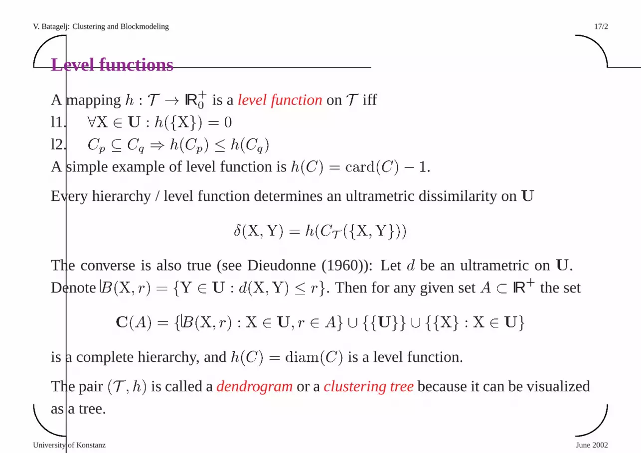
Level functions

A mappingh : T ! IR+0

is a level functiononT iff

l1. 8X 2 U : h(fXg) = 0

l2. C

p

� C

q

) h(C

p

) � h(C

q

)

A simple example of level function ish(C) = ard(C)� 1.

Every hierarchy / level function determines an ultrametricdissimilarity onU

Æ(X;Y) = h(C

T

(fX;Yg))

The converse is also true (see Dieudonne (1960)): Letd be an ultrametric onU.

DenoteB(X; r) = fY 2 U : d(X;Y) � rg. Then for any given setA � IR+ the set

C(A) = fB(X; r) : X 2 U; r 2 Ag [ ffUgg [ ffXg : X 2 Ug

is a complete hierarchy, andh(C) = diam(C) is a level function.

The pair(T ; h) is called adendrogramor aclustering treebecause it can be visualized

as a tree.



&

$%

Association coefficients, Monte Carlo,m = 15

CLUSE – maximum[0:00; 0:33℄

Kulczynski

Driver-KroeberJaccard

Baroni-UrbaniSimpson

Russel-RaoBraun-Blanquet

un

4

Pearson

Michael

Yule

un

5

Sokal-Michener– bc –



&

$%

Inversions

Unfortunately the functionhD

(C) = D(C

p

; C

q

), C = C

p

[ C

q

is not always a level

function – for someDs theinversions,D(Cp

; C

q

) > D(C

p

[ C

q

; C

s

), are possible.

Batagelj (1981) showed:

Theorem 2.3 h

D

is a level function for the Lance-Williams procedure(�1

, �2

, �, )

iff:

(i) +min(�

1

; �

2

) � 0

(ii) �

1

+ �

2

� 0

(iii) �

1

+ �

2

+ � � 1

The dissimilarityD has thereducibility property (Bruynooghe, 1977) iff

D(C

p

; C

q

) � t; D(C

p

; C

s

) � t; D(C

q

; C

s

) � t ) D(C

p

[ C

q

; C

s

) � t

Theorem 2.4 If a dissimilarityD has the reducibility property thenhD

is a level

function.



&

$%

Adding hierarchical methods

Suppose that we already built a clustering treeT over the set of unitsU. To add a new

unitX to the treeT we start in the root and branch down. Assume that we reached

the node corresponding to clusterC, which was obtained by joining subclustersCp

andCq

. There are three possibilities: or to addX toCp

, or to addX toCq

, or to form

a new clusterfXg.

Consider again the ’greedy approximation’P (C

�k

) = P (C

�k+1

) +D(C

p

; C

q

) where

D(C

p

; C

q

) = min

C

u

;C

v

2C

�k+1

D(C

u

; C

v

) andC�i

are greedy solutions.

Since we wish to minimize the value of criterionP it follows from the greedy

relation that we have to select the case corresponding to themaximal among values

D(C

p

[ fXg; C

q

),D(Cq

[ fXg; C

p

) andD(Cp

[ C

q

; fXg).

This is a basis for the adding clustering method. We start with a tree on the first two

units and then successively add to it the remaining units. The unitX is included into

all clusters through which we branch it down.



&

$%

... adding hierarchical methods

t

C

p

t

C

q

t

C

�

��

X

t

C

p

[X

t

C

q

t

C [X

�

��

t

C

p

t

C

q

[X

t

C [X

A

AU

t

C

p

t

C

q

t

C

t

X

t

C [X

H

Hj



&

$%

About the minimal solutions of (Pk

; SR)

Theorem 2.5 In the (locally with respect to transitions) minimal clustering for the

problem(P

k

; SR)

SR: P (C) =

X

C2C

X

X2C

w(X) � d(X; C)

each unit is assigned to the nearest representative: LetC

� be (locally with respect to

transitions) minimal clustering then it holds:

8C

u

2 C

�

8X 2 C

u

8C

v

2 C

�

n fC

u

g : d(X; C

u

) � d(X; C

v

)



&

$%

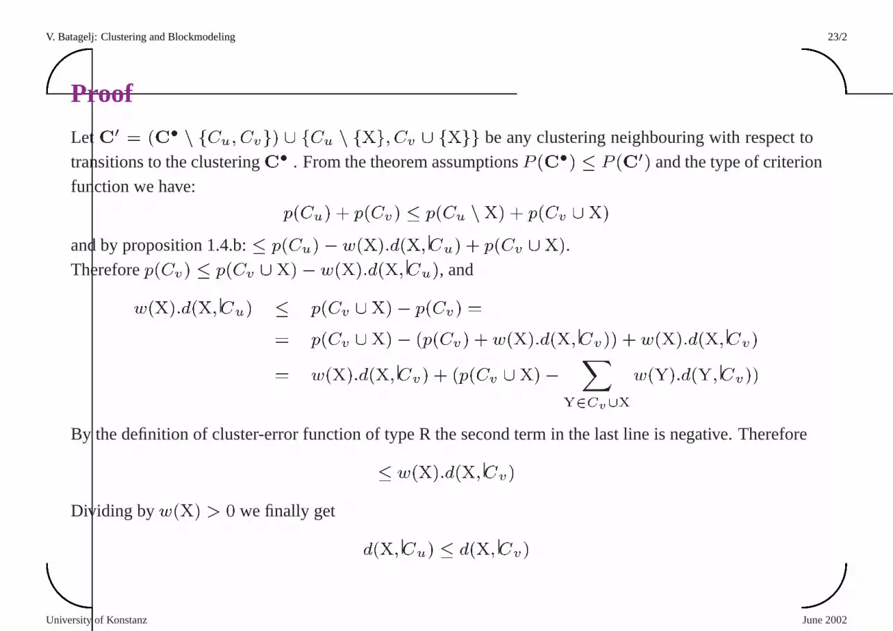
Proof

LetC0

= (C

�

n fC

u

; C

v

g) [ fC

u

n fXg; C

v

[ fXgg be any clustering neighbouring with respect to

transitions to the clusteringC� . From the theorem assumptionsP (C�

) � P (C

0

) and the type of criterion

function we have:

p(C

u

) + p(C

v

) � p(C

u

nX) + p(C

v

[X)

and by proposition 1.4.b:� p(C

u

)� w(X):d(X; C

u

) + p(C

v

[X).

Thereforep(Cv

) � p(C

v

[X)� w(X):d(X; C

u

), and

w(X):d(X; C

u

) � p(C

v

[X)� p(C

v

) =

= p(C

v

[X)� (p(C

v

) + w(X):d(X; C

v

)) + w(X):d(X; C

v

)

= w(X):d(X; C

v

) + (p(C

v

[X)�

X

Y2C

v

[X

w(Y):d(Y; C

v

))

By the definition of cluster-error function of type R the second term in the last line is negative. Therefore

� w(X):d(X; C

v

)

Dividing byw(X) > 0 we finally get

d(X; C

u

) � d(X; C

v

)



&

$%

Leaders methodIn order to support our intuition in further development we shall briefly describe a

simple version of dynamic clusters method – theleadersor k-means method, which is

the basis of the ISODATA program (one among the most popular clustering programs)

and several recent ’data-mining’ methods. In the leaders method the criterion function

has the form SR.

The basic scheme of leaders method is simple:

determineC0

;C := C

0

;

repeatdetermine for eachC 2 C its leaderC;

the new clusteringC is obtained by assigning each unit

to its nearest leader

until leaders stabilize

To obtain a ’good’ solution and an impression of its quality we can repeat this

procedure with different (random)C0

.



&

$%

The dynamic clusters methodThe dynamic clusters method is a generalization of the abovescheme. Let us denote:

� – set ofrepresentatives

L � � – representation

– set offeasible representations

W : ��! IR+0

– extended criterion function

G : ��! – representation function

F : ��! � – clustering function

and



&

$%

Basic scheme of the dynamic clusters method

the following conditions have to be satisfied:

W0. P (C) = min

L2

W (C;L)

the functionsG andF tend to improve (diminish) the value of the extended criterion

functionW :

W1. W (C; G(C;L)) �W (C;L)

W2. W (F (C;L);L) �W (C;L)

then thedynamic clusters methodcan be described by the scheme:

C := C

0

; L := L

0

;

repeat

L := G(C;L);

C := F (C;L)

until the clustering stabilizes



&

$%

Properties of DCM

To this scheme corresponds the sequencev

n

= (C

n

;L

n

); n 2 IN determined by

relationsL

n+1

= G(C

n

;L

n

) and C

n+1

= F (C

n

;L

n+1

)

and the sequence of values of the extended criterion function un

= W (C

n

;L

n

). Let

us also denoteu� = P (C

�

). Then it holds:

Theorem 2.6 For everyn 2 IN, un+1

� u

n

, u� � u

n

,

and if fork > m, vk

= v

m

then8n � m : u

n

= u

m

.

The Theorem 2.6 states that the sequenceu

n

is monotonically decreasing and

bounded, therefore it is convergent. Note that the limit ofu

n

is not necessarilyu� –

the dynamic clusters method is a local optimization method.



&

$%

... types of of DCM sequences

Type A::9k;m 2 IN; k > m : v

k

= v

m

Type B:9k;m 2 IN; k > m : v

k

= v

m

Type B

0

: Type B withk = m+ 1

The DCM sequence(vn

) is of type B if

� sets� and are both finite.

For example, when we select a representative ofC among its members.

� 9Æ > 0 : 8n 2 IN : (v

n+1

6= v

n

) u

n

� u

n+1

> Æ)

Because the setsU and consequently� are finite we expect from a good dynamic

clusters procedure to stabilize in finite number of steps – isof type B.



&

$%

Additional requirement

The conditions W0, W1 and W2 are not strong enough to ensure this. We shall try to

compensate the possibility that the set of representations is infinite by the additional

requirement:

W3. W (C; G(C;L)) =W (C;L)) L = G(C;L)

With this requirement the ’symmetry’ between� and is distroyed. We could

reestablish it by the requirement:

W4. W (F (C;L;L)) =W (C;L)) C = F (C;L)

but it turns out that W4 often fails. For this reason we shall avoid it.

Theorem 2.7 If W3 holds and if there existsm 2 IN such thatum+1

= u

m

, then also

L

m+1

= L

m

.



&

$%

Simple clustering and representation functions

Usually, in the applications of the DCM, the clustering function takes the form

F : ! �. In this case the condition W2 simplifies to:W (F (L);L) � W (C;L)

which can be expressed also asF (L) 2 Min

C2�

W (C;L). For such,simple

clustering functions it holds:

Theorem 2.8 If the clustering functionF is simple and if there existsm 2 IN such

thatLm+1

= L

m

, then for everyn � m : v

n

= v

m

.

What can be said about the case whenG is simple– has the formG : �! ?

Theorem 2.9 If W3 holds and the representation functionG is simple then:

a. G(C) = argmin

L2

W (C;L)

b. 9k;m 2 IN; k > m8i 2 IN : v

k+i

= v

m+i

c. 9m 2 IN8n � m : u

n

= u

m

d. if alsoF is simple then9m 2 IN8n � m : v

n

= v

m



&

$%

Original DCM

In the original dynamic clusters method (Diday, 1979) both functionsF andG are

simple –F : ! � andG : �! .

We proved, if also W3 holds and the functionsF andG are simple, then:

G0. G(C) = argmin

L2

W (C;L)

and

F0. F (L) 2 Min

C2�

W (C;L)

In other words, given an extended criterion functionW , the relations G0 and F0

define an appropriate pair of functionsG andF such that the DCM stabilizes in finite

number of steps.



&

$%

. . . Clustering and NetworksIn the next, 3. lecture we shall discuss

� clustering with relational constraint

� transforming data into graphs (neighbors)

� clustering of networks; dissimilarities between graphs (networks)

� clustering of vertices / links; dissimilarities between vertices

� clustering in large networks


kncourse2: clustering and blockmodeling / 2. approaches to clustering

Documents