arX

iv:a

stro

-ph/

0702

214v

1 7

Feb

200

7SUBMITTED TO AJ ON 3 NOVEMBER 2006Preprint typeset using LATEX style emulateapj v. 10/09/06

CLUSTERING OF HIGH REDSHIFT (Z ≥ 2.9) QUASARS FROM THE SLOAN DIGITAL SKY SURVEY

YUE SHEN1, M ICHAEL A. STRAUSS1, MASAMUNE OGURI1,2, JOSEPHF. HENNAWI3, X IAOHUI FAN4, GORDON T. RICHARDS5,PATRICK B. HALL 6, JAMES E. GUNN1, DONALD P. SCHNEIDER7, ALEXANDER S. SZALAY 8, ANIRUDDA R. THAKAR 8, DANIEL E.

VANDEN BERK7, SCOTT F. ANDERSON9, NETA A. BAHCALL 1, ANDREW J. CONNOLLY10, GILLIAN R. KNAPP1

Submitted to AJ on 3 November 2006

ABSTRACTWe study the two-point correlation function of a uniformly selected sample of 4,426 luminous optical quasars

with redshift 2.9≤ z≤ 5.4 selected over 4041 deg2 from the Fifth Data Release of the Sloan Digital Sky Survey.We fit a power-law to the projected correlation functionwp(rp) to marginalize over redshift space distortionsand redshift errors. For a real-space correlation functionof the formξ(r) = (r/r0)−γ , the fitted parameters incomoving coordinates arer0 = 15.2±2.7h−1 Mpc andγ = 2.0±0.3, over a scale range 4≤ rp ≤ 150h−1 Mpc.Thus high-redshift quasars are appreciably more strongly clustered than theirz≈ 1.5 counterparts, which havea comoving clustering lengthr0 ≈ 6.5 h−1 Mpc. Dividing our sample into two redshift bins: 2.9≤ z≤ 3.5 andz≥ 3.5, and assuming a power-law indexγ = 2.0, we find a correlation length ofr0 = 16.9±1.7h−1 Mpc forthe former, andr0 = 24.3±2.4h−1 Mpc for the latter. Strong clustering at high redshift indicates that quasarsare found in very massive, and therefore highly biased, halos. Following Martini & Weinberg, we relate theclustering strength and quasar number density to the quasarlifetimes and duty cycle. Using the Sheth &Tormen halo mass function, the quasar lifetime is estimatedto lie in the range 4∼ 50 Myr for quasars with2.9≤ z≤ 3.5; and 30∼ 600 Myr for quasars withz≥ 3.5. The corresponding duty cycles are 0.004∼ 0.05 forthe lower redshift bin and 0.03∼ 0.6 for the higher redshift bin. The minimum mass of halos in which thesequasars reside is 2− 3×1012 h−1M⊙ for quasars with 2.9≤ z≤ 3.5 and 4− 6×1012 h−1M⊙ for quasars withz≥ 3.5; the effective bias factorbeff increases with redshift, e.g.,beff ∼ 8 atz= 3.0 andbeff ∼ 16 atz= 4.5.Subject headings:cosmology: observations – large-scale structure of universe – quasars: general – surveys

1. INTRODUCTION

Recent galaxy surveys (e.g., the 2dF Galaxy Redshift Sur-vey, Colless et al. 2001 and the Sloan Digital Sky Survey(SDSS), York et al. 2000) have provided ample data for thestudy of the large-scale distribution of galaxies in the present-day Universe. The clustering of galaxies, which are tracersofthe underlying dark matter distribution, gives a powerful testof hierarchical structure formation theory, especially whencompared with fluctuations in the Cosmic Microwave Back-ground. Indeed, the results show excellent agreement with thenow-standard flatΛ-dominated concordance cosmology (e.g.,Spergel et al. 2003, 2006; Tegmark et al. 2004, 2006; Eisen-stein et al. 2005; Percival et al. 2006). The galaxy two-pointcorrelation function is well-fit by a power law:ξ(r) = (r/r0)−γ

on scalesr . 20 h−1 Mpc, with comoving correlation lengthr0 ∼ 5 h−1 Mpc and slopeγ ∼ 1.8 (Totsuji & Kihara 1969;

1 Princeton University Observatory, Princeton, NJ 08544.2 Kavli Institute for Particle Astrophysics and Cosmology, Stanford Uni-

versity, 2575 Sand Hill Road, Menlo Park, CA 94025.3 Department of Astronomy, Campbell Hall, University of California,

Berkeley, California 947204 Steward Observatory, 933 North Cherry Avenue, Tucson, AZ 85721.5 Department of Physics, Drexel University, 3141 Chestnut Street,

Philadelphia, PA 19104.6 Dept. of Physics & Astronomy, York University, 4700 Keele St.,

Toronto, ON, M3J 1P3, Canada.7 Department of Astronomy and Astrophysics, 525 Davey Laboratory,

Pennsylvania State University, University Park, PA 16802.8 Center for Astrophysical Sciences, Department of Physics and Astron-

omy, Johns Hopkins University, 3400 North Charles Street, Baltimore, MD21218.

9 Department of Astronomy, University of Washington, Box 351580, Seat-tle, WA 98195.

10 Department of Physics and Astronomy, University of Pittsburgh, 3941O’Hara Street, Pittsburgh, PA 15260.

Groth & Peebles 1977; Davis & Peebles 1983; Hawkins et al.2003), although there is an excess above the power law be-low 2h−1 Mpc, thought to be due to halo occupation effects(Zehavi et al. 2004, 2005).

At high redshifts and earlier times, the dark matter cluster-ing strength should be weaker, but the first clustering studiesof high-redshift galaxies with the Keck telescope (Cohen etal.1996; Steidel et al. 1998; Giavalisco et al. 1998; Adelbergeret al. 1998) showed that galaxies atz> 3 show a similar co-moving correlation length to those of today, results that havesince been confirmed with much larger samples (e.g., Adel-berger et al. 2005a; Ouchi et al. 2005; Kashikawa et al. 2006;Meneux et al. 2006; Lee et al. 2006; Quadri et al. 2006). Thisis indeed expected: high-redshift galaxies are thought to format rare peaks in the density field, which will be strongly biasedrelative to the dark matter (Kaiser 1984; Bardeen et al. 1986);under gravitational instability, the bias of galaxies drops overtime as a function of redshift (Tegmark & Peebles 1998; Blan-ton et al. 2000; Weinberg et al. 2004).

Luminous quasars offer a different probe of the clusteringof galaxies at high redshift. Powered by gas accretion ontocentral super-massive black holes (Salpeter 1964; Lynden-Bell 1969), quasars are believed to be the progenitors oflocal dormant super-massive black holes which are ubiqui-tous in the centers of nearby bulge-dominated galaxies (e.g.,Kormendy & Richstone 1995; Magorrian et al. 1998; Yu& Tremaine 2002). Studies of the clustering properties ofquasars date back to Osmer (1981); in general, quasars have aclustering strength similar to that of luminous galaxies atthesame redshift (Shaver 1984; Croom & Shanks 1996; Porciani,Magliocchetti & Norberg 2004, hereafter PMN04; Croom etal. 2005). If the triggering of quasar activity is not tied tothe larger-scale environment in which their host galaxies re-side, this is not a surprising result; quasars are interpreted

2 Y. Shen et al.

as a stochastic process through which every luminous galaxypasses, and therefore the clustering of quasars should be nodifferent from that of luminous galaxies. Studies of the clus-tering of galaxies around quasars similarly find that quasarenvironments are similar to those of luminous galaxies (Ser-ber et al. 2006, and references therein), although evidenceforan enhanced clustering of quasars on small scales (Djorgovski1991; Hennawi et al. 2006a; but see also Myers et al. 2006c)suggests that tidal effects within 100 kpc may trigger quasaractivity.

A number of studies have examined the redshift evolutionof quasar clustering, but the results have been controversial:some papers conclude that quasar clustering either decreasesor weakly evolves with redshift (e.g., Iovino & Shaver 1988;Croom & Shanks 1996), while others say that it increases withredshift (e.g., Kundic 1997; La Franca et al. 1998; PMN04;Croom et al. 2005). Myers et al. (2006a, b, c) examinedthe clustering of quasar candidates with photometric redshiftsfrom the SDSS; they find little evidence for evolution in clus-tering strength betweenz≈ 2 and today. These studies alsofind little evidence for a strong luminosity dependence of thequasar correlation function (e.g., Croom et al. 2005; Connollyet al., in preparation), which is in accord with quasar modelsin which quasar luminosity is only weakly related to blackhole mass (Lidz et al. 2006).

The vast majority of quasars in flux-limited samples likethe SDSS (and especially UV-excess surveys like the 2dFQSO Redshift Survey; Croom et al. 2004) are at relativelylow redshift,z < 2.5. More distant quasars are intrinsicallyrarer (e.g., Richards et al. 2006), and at a given luminosityare of course substantially fainter. However, we might expecthigh-redshift quasars to be appreciably more biased than theirlower-redshift counterparts. The high-redshift quasars in flux-limited samples are intrinsically luminous, and by the Ed-dington argument, are powered by massive (> 108M⊙) blackholes. If the relation between black hole mass and bulge mass(Tremaine et al. 2002 and references therein), and by exten-sion, black hole mass and dark matter halo mass (Ferrarese2002) holds true at high redshift, then luminous quasars re-side in very massive, and therefore very rare halos at highredshift. Rare, many−σ peaks in the density field are stronglybiased (Bardeen et al. 1986). Thus detection of particularlystrong clustering at high redshift would allow tests both ofthe relationship between quasars and their host halos, andthe predictions of biasing models. The rarity of the halos inwhich quasars reside is of course related to the observed num-ber density of quasars and their duty cycle/lifetime, thus thequasar luminosity function and the quasar clustering proper-ties can be used to constrain the average quasar lifetimetQ(Haiman & Hui 2001; Martini & Weinberg 2001), or equiv-alently, the duty cycle: the fraction of time a supermassiveblack hole shines as a luminous quasar.

Studies to date of the clustering of high-redshift quasarshave been hampered by small number statistics. Stephens etal. (1997) and Kundic (1997) examined threez> 2.7 quasarpairs with comoving separations 5− 10 h−1 Mpc in the Palo-mar Transit Grism Survey of Schneider et al. (1994), and esti-mated a comoving correlation lengthr0 ∼ 17.5±7.5h−1 Mpc,which is three times higher than that of lower redshift quasars.Schneider et al. (2000) found a pair ofz = 4.25 quasars inthe SDSS separated by less than 2h−1 Mpc; this single pairimplies a lower limit to the correlation length ofr0 = 12 h−1

Mpc. Similarly, the quasar pair separated by a few Mpc atz∼ 5 found by Djorgovski et al. (2003) also implies strong

clustering at high redshift. However, measuring a true corre-lation function requires large samples of quasars. Atz∼ 4,the mean comoving distance between luminous (Mi < −27.6)quasars is∼ 150 h−1 Mpc (Fan et al. 2001; Richards et al.2006), thus to build up statistics on smaller-scale clustering insuch a sparse sample requires a very large volume. The SDSSquasar sample is the first survey of high-redshift quasars thatcovers enough volume to allow this measurement to be made.

This paper presents the correlation function of high redshift(z≥ 2.9) quasars using the fifth data release (DR5; Adelman-McCarthy et al. 2007) of the SDSS. DR5 contains∼ 6,000quasars with redshiftz≥ 2.9. We construct a homogeneousflux-limited sample for clustering analysis in § 2, with spe-cial focus on redshift determination in Appendix A, and theangular mask of the sample in Appendix B. We present thecorrelation function itself in § 3, together with a discussion ofits implications for quasar duty cycles and lifetimes. We con-clude in Section 4. Throughout the paper we use the third yearWMAP + all parameters11 (Spergel et al. 2006) for the cosmo-logical model:ΩM = 0.26,ΩΛ = 0.74,Ωb = 0.0435,h = 0.71,ns = 0.938,σ8 = 0.751. Comoving units are used in distancemeasurements; for comparison with previous results, we willoften quote distances in units ofh−1 Mpc.

2. SAMPLE SELECTION

2.1. The SDSS Quasar Sample

The SDSS uses a dedicated 2.5-m wide-field telescope(Gunn et al. 2006) which uses a drift-scan camera with 302048×2048 CCDs (Gunn et al. 1998) to image the sky in fivebroad bands (ugr iz; Fukugita et al. 1996). The imaging dataare taken on dark photometric nights of good seeing (Hogget al. 2001), are calibrated photometrically (Smith et al. 2002;Ivezic et al. 2004; Tucker et al. 2006) and astrometrically (Pieret al. 2003), and object parameters are measured (Lupton et al.2001; Stoughton et al. 2002). Quasar candidates (Richards etal. 2002b) for follow-up spectroscopy are selected from theimaging data using their colors, and are arranged in spectro-scopic plates (Blanton et al. 2003) to be observed with a pairof double spectrographs. The quasars observed through theThird Data Release (Abazajian et al. 2005) have been cata-loged by Schneider et al. (2005), while Schneider et al. (2006)extend this catalog to the DR5. In this paper, we will use re-sults from DR5, for which spectroscopy has been carried outover 5740 deg2. Because of the diameter of the fiber cladding,two targets on the same plate cannot be placed closer than 55′′

(corresponding to∼ 1.2 h−1 Mpc atz= 3)12; the present papertherefore concentrates on clustering on larger scales, andwewill present a discussion of the correlation function on smallscales in a paper in preparation.

The quasar target selection algorithm is in two parts:quasars withz≤ 3.5 are outliers from the stellar locus in theugri color cube, while those withz> 3.5 are selected as out-liers in thegriz color cube. The quasar candidate sample isflux-limited to i = 19.1 (after correction for Galactic extinc-tion following Schlegel, Finkbeiner, & Davis 1998), but be-cause high-redshift quasars are quite rare, the magnitude limitfor objects lying in those regions of color space correspondingto quasars atz> 3 are targeted toi = 20.2. The quasar locuscrosses the stellar locus in color space atz≈ 2.7 (Fan 1999),meaning that quasar target selection is quite incomplete there

11 http://lambda.gsfc.nasa.gov/product/map/current/params/lcdm_all.cfm12 Serendipitous objects closer than 55′′ might be observed on overlapped

plates.

Quasar Correlation Function atz≥ 2.9 3

(Richards et al. 2006). For this reason, we have chosen todefine high-redshift quasars as those withz≥ 2.9.

We draw our parent sample from the SDSS DR5 catalog.We have taken all quasars with listed redshiftz≥ 2.9 fromthe DR3 quasar catalog (Schneider et al. 2005); the redshiftsof these objects have all been checked by eye, and we rec-tify a small number of incorrect redshifts in the database.This sample contains 3,333 quasars. In addition, we haveincluded all objects on plates taken since DR3 with listedredshiftz≥ 2.9 as determined either from the official spec-troscopic pipeline which determines redshifts by measuringthe position of emission lines (SubbaRao et al. 2002) or anindependent pipeline which fits spectra to quasar templates(Schlegel et al., in preparation). We examined by eye thespectra of all objects with discrepant redshifts between thetwo pipelines. There are 2,805 quasars added to our samplefrom plates taken since DR3.

Quasar emission lines are broad, and tend to show system-atic wavelength offsets from the true redshift of the object(Richards et al. 2002a and references therein). Appendix Adescribes our investigation of these effects, determination ofan unbiased redshift for each object, and the definition of ourfinal sample of 6,109 quasars withz≥ 2.9 (after rejecting 29objects that turn out to havez< 2.9).

2.2. Clustering Subsample

Not all the quasars in our sample are suitable for a cluster-ing analysis. Here we follow Richards et al. (2006) and selectonly those quasars that are selected from a uniform algorithm.In particular:

• The version of the quasar target selection algorithmused for the SDSS Early Data Release (Stoughton et al.2002) and the First Data Release (DR1; Abazajian et al.2003) did a poor job of selecting objects withz≈ 3.5.We use only those quasars targeted with the improvedversion of the algorithm, i.e., those with target selectionversion no lower than v3_1_0.

• Some quasars are found using algorithms other than thequasar target selection algorithm described by Richardset al. (2002b), including special selection in the South-ern Galactic Cap (see Adelman-McCarthy et al. 2006)and optical counterparts to ROSAT sources (Andersonet al. 2003). The completeness of these auxiliary algo-rithms is poor, and we only include quasars targeted bythe main algorithm.

• Because quasars are selected by their optical colors, re-gions of sky in which the SDSS photometry is poor areunlikely to have complete quasar targeting.

We now describe how the regions with poor photometry areidentified. The SDSS images are processed in a series of 10′×13′ fields. We follow Richards et al. (2006) and mark a givenfield has having bad photometry if any one of the followingcriteria is satisfied:

• ther-band seeing is greater than 2′′.0;

• The operational database quality flag for that field isBAD, MISSING or HOLE (only 0.15% of all DR5fields have one of these flags set);

• The median difference between the PSF and large-aperture photometry magnitudes of bright stars lies

more than 3σ from the mean over the entire DR5 sam-ple in any of the five bands;

• Any of the four principal colors of the stellar locus(Ivezic et al. 2004) deviates from the mean of the DR5sample by more than 3σ;

• Any of the four values of the rms scatter around themean principal color deviates from the mean over DR5by more than 5σ, or, deviates from the DR5 mean bymore than 2σ, and also deviates from the mean of thatrun by more than 3σ. This criterion reflects the factthat the statistics of the rms widths of the principal colordistributions per field vary significantly from run to run.

All the information we need to identify bad fields in this waycan be retrieved from therunQA table in the SDSS CatalogueArchive Server (CAS13). A total of 13.24% of the net area ofthe clustering subsample is marked as bad. These bad fieldswill serve as a secondary mask in our geometry description.We will compute the correlation function both including andexcluding the bad regions, to test our sensitivity to possibleselection problems in the bad regions.

Finally, due to overlapping plates, there are roughly 200duplicate objects in our parent sample, which we identifiedand removed using objects’ positions.

Our final cleaned subsample contains 4,426 quasars beforeexcluding bad fields and 3,846 quasars with bad fields ex-cluded. Thus 13.1% of high-redshift quasars are in bad fields,essentially identical to the fraction of the area flagged as bad,which suggests that the selection of quasars in these regions isnot terribly biased. A list of the unique high-redshift quasarsin our parent sample and in the subsample used in our cluster-ing analysis is provided in Table 1.

2.3. Distribution of Quasars in Angle and on the Sky

The footprint of our quasar clustering subsample is quitecomplicated. The definition of the sample’s exact boundaries,needed for the correlation function analysis which follows,is described in detail in Appendix B. Fig. 1 shows the areaof sky from which the sample was selected in green, and thesample of quasars is indicated as dots, with red dots indicatingobjects in bad imaging fields. The total area subtended by thesample is 4041 deg2; when bad fields are excluded, the solidangle drops to 3506 deg2.

The target selection algorithm for quasars is not perfect andthe selection function depends on redshift. Our sample is lim-ited toz≥ 2.9; at slightly lower redshift, the broad-band col-ors of quasars are essentially identical to those of F stars (Fan1999), giving a dramatic drop in the quasar selection function.Moreover, as discussed in Richards et al. (2006), quasars withredshiftz≈ 3.5 have similar colors to G/K stars in thegriz di-agram and hence targeting becomes less efficient around thisredshift (as mentioned above, this problem was even worse forthe version of target selection used in the EDR and DR1). Thisis reflected in the redshift distribution of our sample (Fig.2),which shows a dip atz≈ 3.5. We will use these distributionsin computing the correlation function below.

3. CORRELATION FUNCTION

Now that we understand the angular and radial selectionfunction of our sample, we are ready to compute the two-point

13 http://cas.sdss.org

4 Y. Shen et al.

TABLE 1HIGH REDSHIFT QUASAR SAMPLE

Plate Fiber MJD RA (deg) DEC (deg) z zerr i mag sub_flag good_flag

1091 553 52902 0.193413 1.239112 3.741 0.011 19.74 0 01489 506 52991 0.214856 0.200710 3.881 0.030 19.97 0 01489 104 52991 0.397978 −0.701886 3.572 0.008 19.33 0 00387 556 51791 0.587972 0.363741 3.057 0.010 18.58 0 00650 111 52143 0.660070 −10.197168 3.942 0.012 19.97 0 00750 608 52235 0.751425 16.007709 3.689 0.011 19.50 1 10650 048 52143 0.763943 −10.864079 3.645 0.011 19.20 0 00750 036 52235 0.896718 14.795454 3.462 0.012 19.95 1 10750 632 52235 1.155146 15.174562 3.203 0.009 20.17 1 10751 207 52251 1.401625 13.997071 3.705 0.011 19.34 1 1

NOTE. — The entire high redshift quasar sample with duplicate objects removed. Thesub_flagis 1 when an object is in the clustering subsample, and thegood_flagis 1 for objects lying in good fields. Thei magnitudes are SDSS PSF (asinh) magnitudes corrected for Galactic extinction (Schlegel et al. 1998); theyuse the ubercalibration described by Padmanabhan et al. (2007), which differs slightly from that used in the official DR5quasar catalog (Schneider et al. 2007).The entire table is available in the electronic edition of the paper.

FIG. 1.— Aitoff projection in equatorial coordinates of the angular coverage of our clustering subsample (with all fields).The center of the plot is the directionRA = 120 and Dec = 0. The dots indicate quasars in our clustering subsample, with red dots indicating those in bad imaging fields. The angularcoverage ispatchy due to the various selection criteria described in §2.2 and Appendix B. For example, much of the Southern Equatorial Stripe (δ = 0, 300< α < 60) wastargeted using the old version of the quasar targetting algorithm.

correlation function. Doing so requires producing a randomcatalog of points (i.e., without any clustering signal) with thesame spatial selection function. We will first compute the cor-relation function in “redshift space” in § 3.1, then derive thereal-space correlation function in § 3.2 by projecting overred-shift space distortions. Our calculations will be done bothin-cluding and excluding the bad fields (§ 2.2); we will find thatour results are robust to this detail.

3.1. “Redshift Space” Correlation Function

We draw random quasar catalogs according to the detailedangular and radial selection functions discussed in the lastsection.

We start by computing the correlation function in “redshiftspace”, where each object is placed at the comoving distanceimplied by its measured redshift and our assumed cosmology,

with no correction for peculiar velocities or redshift errors14.The correlation function is measured using the estimator ofLandy & Szalay (1993)15:

ξs(s) =〈DD〉− 2〈DR〉+ 〈RR〉

〈RR〉 , (1)

where 〈DD〉, 〈DR〉, and 〈RR〉 are the normalized numbersof data-data, data-random and random-random pairs in eachseparation bin, respectively. The results are shown in Fig.3,where we bin the redshift space distances in logarithmic in-tervals of∆ log10s= 0.1. We tabulate the results in Table 2.

There are various ways to estimate the statistical errors in

14 All calculations in this paper are done in comoving coordinates, whichis appropriate for comparing clustering results at different epochs on linearscales. On very small, virialized scales, Hennawi et al. (2006a) argue thatproper coordinates are more appropriate for clustering analyses.

15 We found that the Hamilton (1993) estimator gives similar results.

Quasar Correlation Function atz≥ 2.9 5

FIG. 2.— Observed redshift distribution of our quasar clustering subsam-ples, normalized by the peak value. This distribution is theproduct of theevolution of the quasar density distribution, and the quasar selection func-tion; the latter is responsible for the dip atz ≈ 3.5, where quasars have verysimilar colors to those of G and K stars. We show the redshift distributionsfor the subsamples both including and excluding bad fields; the results areessentially identical. The redshift binning is∆z= 0.05.

TABLE 2REDSHIFT SPACE CORRELATION FUNCTIONξs(s)

s (h−1 Mpc) DDmean RRmean DRmean ξs ξs error

2.244 0.0 0.9 0.0 – –2.825 0.0 5.4 0.0 – –3.557 0.0 6.3 0.0 – –4.477 1.8 14.4 0.9 16.5 12.85.637 0.0 34.2 3.6 – –7.096 1.8 38.7 11.7 3.54 3.618.934 1.8 99.0 18.0 1.26 1.8811.25 2.7 215.0 36.9 0.663 0.73314.16 4.5 406.5 80.0 0.191 0.78617.83 8.9 804.2 162.4 0.131 0.47222.44 15.2 1592.4 279.4 0.236 0.17528.25 22.4 3123.6 607.3 −0.280 0.22335.57 70.7 6028.6 1139.3 0.361 0.17044.77 104.9 11959.1 2137.1 0.101 0.12156.37 210.9 23480.2 4381.2 0.0384 0.086270.96 384.8 45648.7 8239.8 0.0368 0.064489.34 734.2 88337.9 16036.1 0.0101 0.0382112.5 1417.1 168480.9 30636.2 0.0194 0.0250141.6 2565.8 317727.8 57230.3−0.00396 0.0219178.3 4821.6 588892.8 106083.7 0.0101 0.0134224.4 8631.8 1070807.1 192603.7−0.00296 0.00672282.5 15376.1 1912774.1 342706.1 0.00214 0.00953

NOTE. — Result for all fields. DDmean, RRmeanand DRmeanare the meannumbers of quasar-quasar , random-random and quasar-random pairs withineachs bin for the ten jackknife samples.ξ(s) is the mean value calculatedfrom jackknife samples, and the error quoted is that from thejackknifes aswell.

the correlation function (e.g., Hamilton 1993), includingboot-strap resampling (e.g., PMN04), jackknife resampling (e.g.,Zehavi et al. 2005), and the Poisson estimator (e.g., Croomet al. 2005; da Ângela et al. 2005). In this paper we will fo-cus on the latter two methods. For the jackknife method, wesplit the clustering sample into 10 spatially contiguous sub-samples, and our jackknife samples are created by omittingeach of these subsamples in turn. Therefore, each of the jack-knife samples contains 90% of the quasars, and we use each tocompute the correlation function. The covariance error matrix

is estimated as

Cov(ξi , ξ j ) =N − 1

N

N∑

l=1

(

ξli − ξi

)(

ξlj − ξ j

)

, (2)

whereN = 10 in our case, the subscript denotes the bin num-ber, andξi is the mean value of the statisticξi over the jack-knife samples (not surprisingly, we found thatξi was veryclose to the correlation function for the whole clustering sam-ple, for all binsi). Our sample is sparse, thus the off-diagonalelements of the covariance matrix are poorly determined, sowe use only the diagonal elements of the covariance matrixin the χ2 fits below. We also carried out fits keeping thoseoff-diagonal elements for adjacent and separated-by-two bins,and found similar results.

For the Poisson error estimator (e.g., Kaiser 1986), validfor sparse samples in which a given quasar is unlikely totake part in more than one pair, the error is estimated as∆ξi = (1+ ξi)/

√

Min(Npair,NQSO), whereNpair is the numberof unique quasar-quasar pairs in our real quasar sample in thebin in question, andNQSO is the total number of real quasars inour sample (e.g., da Ângela et al. 2005). The Poisson estima-tor breaks down on large scales, as the pairs in different binsbecome correlated. Fig. 3 shows the two error estimators; thetwo methods give similar results.

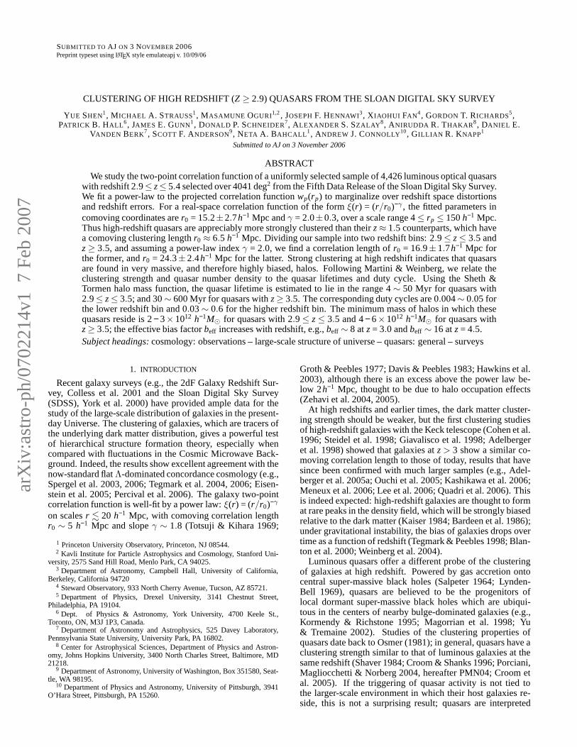
The correlation function lies above unity for scales below∼ 10 h−1 Mpc; it is clear that the clustering signal is muchstronger than that of low-redshift quasars (e.g., Croom et al.2005; Connolly et al. 2006). Fig. 3 also shows the results ofaχ2 fit of a power-law correlation functionξs(s) = (s/s0)−δ tothe data with 4< s< 150h−1 Mpc. The clustering signal isnegative in thes= 28.25 h−1Mpc bin; Table 2 shows a smallernumber of quasar-quasar pairs than expected. This point ap-pears to be an outlier, as the expected correlation functionshould be positive on these scales; this discrepancy may bedue to the paucity of quasars in the sample atz∼ 3.5. Wehave carried out fits toξs(s) both including and not includingthis data point (Table 4); we find it makes little difference.In particular, neglecting the point at 28.25h−1 Mpc, we finds0 = 10.2± 3.1 h−1 Mpc andδ = 1.71± 0.43 for the Poissonerrors, ands0 = 10.4± 3.0 h−1 Mpc andδ = 1.73± 0.46 forthe jackknife method. When we include this negative datapoint, we finds0 = 10.4 h−1Mpc andδ = 2.07 for the jack-knife method. Table 4 also includes theχ2/dof for these fits;in all cases, it is less than unity, due to our neglecting theoff-diagonal elements in the covariance matrix. However, asFigure 3 makes clear, the majority of the points lie within 1sigma of the fitted power law.

Using good fields only yields similar results for bins wherethere are more than 20 real quasar pairs (i.e.,s& 20h−1 Mpc).On scales below 20h−1 Mpc there are very few quasar-quasarpairs in each bin, and the signal-to-noise ratio is very low.The fitting results (over scale range 4< s< 150h−1 Mpc) are:s0 = 12.7± 3.3 h−1 Mpc andδ = 1.64± 0.31 for the Poissonerrors;s0 = 10.3± 3.0 h−1 Mpc andδ = 1.43± 0.28 for thejackknife errors.

To study the large scale behavior ofξs(s) we computeξs(s)up to s = 2000h−1 Mpc on a linear grid with∆s = 20 h−1

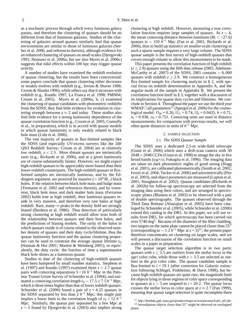
Mpc, using all the fields. The result is shown in Fig. 4 anderrors are estimated using the Poisson estimator. For scales200< s < 2000 h−1Mpc, the mean value ofξs(s) is 0.002,with an rms scatter of±0.01 (see also Roukema, Mamon &Bajtlik 2002 and Croom et al. 2005). Thus there is no clearevidence for correlations on scales above 200h−1 Mpc.

6 Y. Shen et al.

FIG. 3.— Redshift space correlation functionξs(s) for quasars withz≥ 2.9 (all fields included). Statistical errors are estimated using the Poisson estimator(left) and jackknife estimator (right). The two estimators give comparable results. Also plottedare the best fitted power-law functions, with fitted parameterslisted in Table 4.

FIG. 4.— Large scale behavior ofξs(s) for the z≥ 2.9 quasars (all fields included). Errors are estimated using the Poisson estimator. The redshift spacecorrelation function essentially vanishes afters> 200h−1 Mpc, with a mean of 0.002 and rms scatter±0.01 in the range 200< s< 2000h−1 Mpc.

3.2. The Real Space Correlation Function

Appendix A shows that the uncertainty in measurementsof the quasar redshifts is substantial,∆z≈ 0.01, giving anuncertainty in the comoving distance of az = 3.5 quasar of∼ 6 h−1 Mpc. This, together with peculiar velocities on largeand small scales systematically bias the correlation function(e.g., Kaiser 1987). To determine the real-space correlationfunction, we follow standard practice and compute the corre-lation function on a two-dimensional grid of pair separationsparallel (π) and perpendicular (rp) to the line of sight. Ourgrid has a logarithmic increment of 0.15 along therp directionand a linear increment of 5h−1 Mpc along theπ direction. Asabove, the two dimensional correlation functionξs(rp,π) isestimated using the Landy & Szalay (1993) estimator, equa-tion (1). Redshift errors and peculiar velocities affect the sep-aration along theπ direction but not along therp direction.

Therefore we project out these effects by integratingξs(rp,π)along theπ direction to obtain the projected correlation func-tion wp(rp):

wp(rp) = 2∫ ∞

0dπξs(rp,π) . (3)

In practice we integrate up to some cutoff value ofπcutoff =100 h−1 Mpc, which includes most of the clustering signal,without being dominated by noise. This value ofπcutoff islarger than the values of 40− 70 h−1 Mpc typically used inclustering analyses for galaxies and low-redshift quasars(e.g.,Zehavi et al. 2005, PMN04, da Ângela et al. 2005) because ofthe substantially stronger clustering of high-redshift quasars.We verify that our results are not sensitive to the precise valueof πcutoff we adopt.

The projected correlation functionwp is related to the real-

Quasar Correlation Function atz≥ 2.9 7

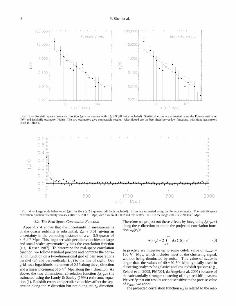
FIG. 5.— Projected correlation functionwp(rp) for the z≥ 2.9 quasars. Errors are estimated using the jackknife method.Also plotted are the best fittedpower-law functions, with fitted parameters listed in Table4. left: for all fields;right: for good fields only. The two cases give similar results.

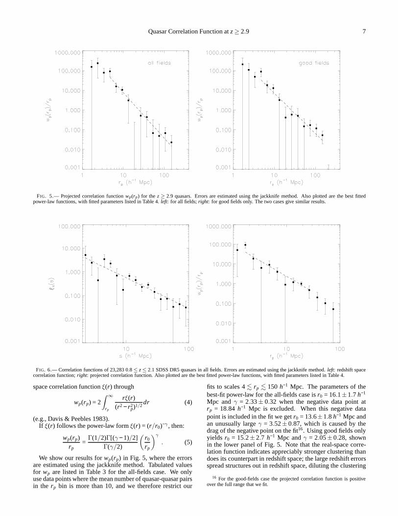
FIG. 6.— Correlation functions of 23,283 0.8 ≤ z≤ 2.1 SDSS DR5 quasars in all fields. Errors are estimated using the jackknife method.left: redshift spacecorrelation function;right: projected correlation function. Also plotted are the bestfitted power-law functions, with fitted parameters listed inTable 4.

space correlation functionξ(r) through

wp(rp) = 2∫ ∞

rp

rξ(r)(r2 − r2

p)1/2dr (4)

(e.g., Davis & Peebles 1983).If ξ(r) follows the power-law formξ(r) = (r/r0)−γ , then:

wp(rp)rp

=Γ(1/2)Γ[(γ − 1)/2]

Γ(γ/2)

(

r0

rp

)γ

. (5)

We show our results forwp(rp) in Fig. 5, where the errorsare estimated using the jackknife method. Tabulated valuesfor wp are listed in Table 3 for the all-fields case. We onlyuse data points where the mean number of quasar-quasar pairsin the rp bin is more than 10, and we therefore restrict our

fits to scales 4. rp . 150 h−1 Mpc. The parameters of thebest-fit power-law for the all-fields case isr0 = 16.1±1.7 h−1

Mpc andγ = 2.33± 0.32 when the negative data point atrp = 18.84 h−1 Mpc is excluded. When this negative datapoint is included in the fit we getr0 = 13.6±1.8 h−1 Mpc andan unusually largeγ = 3.52± 0.87, which is caused by thedrag of the negative point on the fit16. Using good fields onlyyields r0 = 15.2± 2.7 h−1 Mpc andγ = 2.05± 0.28, shownin the lower panel of Fig. 5. Note that the real-space corre-lation function indicates appreciably stronger clustering thandoes its counterpart in redshift space; the large redshift errorsspread structures out in redshift space, diluting the clustering

16 For the good-fields case the projected correlation functionis positiveover the full range that we fit.

8 Y. Shen et al.

FIG. 7.— Clustering evolution of high redshift quasars. Errorsare estimated using the jackknife method. Black indicates the 2.9≤ z≤ 3.5 bin and red indicatesthez≥ 3.5 bin. Also plotted are the best fitted power-law functions, with fitted parameters listed in Table 4.left: all fields; right: good fields only. Both casesshow stronger clustering in the higher redshift bin.

TABLE 3PROJECTED CORRELATION FUNCTIONwp(rp)

rp (h−1 Mpc) DDmean RRmean DRmeanwprp

wprp

error

1.189 0.0 114.3 19.8 – –1.679 0.9 258.3 39.6 154 1622.371 4.5 478.5 91.8 236 1953.350 9.9 913.2 160.8 78.1 51.54.732 20.7 1864.1 359.9 91.3 41.66.683 32.4 3786.5 684.3 15.7 7.819.441 62.9 7158.5 1314.0 10.6 4.4513.34 130.0 14551.2 2659.1 3.06 2.8518.84 227.3 28598.1 5162.4 -0.681 0.91326.61 488.5 56940.7 10123.8 0.516 0.81037.58 871.7 111284.0 19955.6 0.437 0.39553.09 1762.2 218346.8 38910.9 0.0675 0.25974.99 3394.4 422580.9 75630.1 0.0484 0.145105.9 6751.7 811406.0 145785.5 0.0674 0.0592149.6 12425.7 1535320.8 274851.9 0.0228 0.0292211.3 22655.1 2849970.6 509877.9 -0.0183 0.00992

NOTE. — Result for all fields. DDmean, DRmean, and RRmean arethe mean numbers of quasar-quasar, random-random and quasar-randompairs within eachrp bin for the ten jackknife samples.wp(rp)/rp is themean value calculated from the jackknife samples.

signal.We have already indicated that the clustering signal is ap-

preciably stronger than at lower redshift. To check that thiswas not somehow an artifact of our processing we selecteda sample of 23,283 spectroscopically confirmed quasars with0.8 ≤ z≤ 2.1 from the SDSS DR5, with the same selectioncriteria as we used above (§ 2.2). Figure 6 shows the re-sultingξs(s) andwp(rp); to compare with the results of otherauthors (e.g., da Ãngela et al. 2005; Connolly et al. 2006),we integrated toπcutoff = 70 h−1 Mpc. We fit power-lawsover the range 1< s < 100 h−1 Mpc (Croom et al. 2005)for ξs(s), and 1.2 < rp < 30 h−1 Mpc for wp(rp) (PMN04and da Ângela et al. 2005). The fitted power-law parame-ters are:s0 = 6.36± 0.89 h−1 Mpc andδ = 1.29± 0.14 forξs(s); r0 = 6.47±1.55h−1 Mpc andγ = 1.58±0.20 forwp(rp).These results are in excellent agreement with Croom et al.

(2005), PMN04 and da Ângela et al. (2005) based on the 2QZsample, and Connolly et al. (2006) based on the SDSS sam-ple. Note that the 2QZ papers use a slightly different cosmol-ogy, which causes very little difference. More importantly,the 2QZ sample is at lower mean luminosity than the SDSSsample, although there is only a mild luminosity dependenceof the clustering strength (e.g., Lidz et al. 2006; Connollyetal. 2006). We note that the amplitude ofwp(rp) for rp & 30h−1 Mpc is lower than predicted from the power-law fit, whichis also the case in da Ângela et al. (2005, Fig. 2).

The predicted correlation function of the underlying darkmatter atr = 15 h−1 Mpc is ∼ 0.014 atz = 3.5 (see §3.3 andAppendix C), far below that of the current high redshift quasarsample (Fig. 5), indicating that our high-redshift quasar sam-ple is very strongly biased.

The increase in clustering signal with redshift we have seensuggests that we may be able to see redshift evolutionwithinour sample. We divide our clustering sample into two sub-samples with redshift intervals 2.9≤ z≤ 3.5 andz≥ 3.5. Theresultingwp(rp) are shown in Fig. 7. The higher redshift binshows systematically stronger clustering than does the lowerredshift bin. The fitted parameters are:r0 = 16.0± 1.8 h−1

Mpc andγ = 2.43±0.43 for 2.9≤ z≤ 3.5; andr0 = 22.5±2.5h−1 Mpc andγ = 2.28± 0.31 for z≥ 3.5, where the fittingrange is 4∼ 150 h−1 Mpc. Using good fields only yields:r0 = 17.9±1.5 h−1 Mpc andγ = 2.37±0.29 for 2.9≤ z≤ 3.5;r0 = 25.2±2.5h−1 Mpc andγ = 2.14±0.24 forz≥ 3.5. Whenwe fix the power-law index to beγ = 2.0 we get slightly dif-ferent but consistent correlation lengths for each case (Table4). Indeed, the clustering of quasars increases strongly withredshift over the range probed by our sample.

The increase in clustering strength with redshift may be dueto two effects: an ever-increasing bias of the halos hostingquasars with fixed luminosity with redshift, and luminosity-dependent clustering. The higher-redshift quasars are moreluminous (Table 6 and Fig. 17 of Richards et al. 2006), andmay be associated with more massive haloes. At low red-shift (z. 3) and moderate luminosities, luminosity dependson accretion rate as much as black hole mass, and one expects

Quasar Correlation Function atz≥ 2.9 9

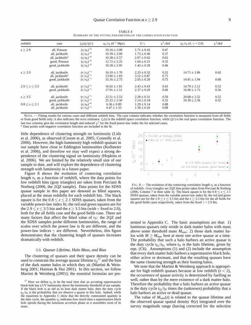
TABLE 4SUMMARY OF THE FITTING PARAMETERS OF THE CORRELATION FUNCTION

redshift case ξs(s)/ξ(r) s0/r0 (h−1 Mpc) δ/γ χ2/dof s0/r0 (δ, γ = 2.0) χ2/dof

z≥ 2.9 all, Poisson (s/s0)−δ 10.16±3.08 1.71±0.43 0.47all, jackknife (s/s0)−δ 10.39±3.00 1.73±0.46 0.37all, jackknifea (s/s0)−δ 10.38±2.57 2.07±0.62 0.62good, Poisson (s/s0)−δ 12.72±3.25 1.64±0.31 0.35

good, jackknife (s/s0)−δ 10.28±2.95 1.43±0.28 0.46

z≥ 2.9 all, jackknife (r/r0)−γ 16.10±1.70 2.33±0.32 0.32 14.71±1.86 0.42all, jackknifea (r/r0)−γ 13.60±1.83 3.52±0.87 0.75

good, jackknife (r/r0)−γ 15.16±2.75 2.05±0.28 0.75 14.81±1.94 0.68

2.9≤ z≤ 3.5 all, jackknife (r/r0)−γ 16.02±1.81 2.43±0.43 0.43 14.79±2.12 0.52good, jackknife (r/r0)−γ 17.91±1.51 2.37±0.29 0.46 16.90±1.73 0.56

z≥ 3.5 all, jackknife (r/r0)−γ 22.51±2.53 2.28±0.31 0.50 20.68±2.52 0.52good, jackknife (r/r0)−γ 25.22±2.50 2.14±0.24 0.32 24.30±2.36 0.32

0.8≤ z≤ 2.1 all, jackknife (s/s0)−δ 6.36±0.89 1.29±0.14 0.88all, jackknife (r/r0)−γ 6.47±1.55 1.58±0.20 0.88

NOTE. — Fitting results for various cases and different redshiftbins. Thecasecolumn indicates whether the correlation function is measured from all fieldsor from good fields only; it also indicates the error estimator. ξs(s) is the redshift space correlation function, whileξ(r) is the real space correlation function. Thelast two columns give the correlation length and reducedχ2 for the fixed power-law index fits for selected cases.a Data points with negative correlation function are included in the fit.

little dependence of clustering strength on luminosity (Lidzet al. 2006), as observed (Croom et al. 2005; Connolly et al.2006). However, the high-luminosity high redshift quasarsinour sample have close to Eddington luminosities (Kollmeieret al. 2006), and therefore we may well expect a strong de-pendence of the clustering signal on luminosity (Hopkins etal. 2006). We are limited by the relatively small size of oursample to date, and will explore the dependence of clusteringstrength with luminosity in a future paper.

Figure 8 shows the evolution of comoving correlationlengthr0 as a function of redshift, where the data points forlow redshift bins (gray triangles) are taken from Porciani &Norberg (2006, the 2QZ sample). Data points for the SDSSquasar sample in this paper are denoted as filled squares,placed at the mean redshifts for each redshift bin. The blacksquare is for the 0.8≤ z≤ 2.1 SDSS quasars, taken from thevariable power-law index fit; the red and green squares are forthe 2.9≤ z≤ 3.5 bin and thez≥ 3.5 bin (withγ fixed to 2.0),both for the all fields case and the good fields case. There aremany factors that affect the fitted value ofr0: the 2QZ andthe SDSS samples probe different luminosities, the range ofscales over which the power law is fit are different, and thepower-law indicesγ are different. Nevertheless, this figuredemonstrates that the clustering length of quasars increasesdramatically with redshift.

3.3. Quasar Lifetime, Halo Mass, and Bias

The clustering of quasars and their space density can beused to constrain the average quasar lifetimetQ17 and the biasof the dark matter halos in which they sit (Martini & Wein-berg 2001; Haiman & Hui 2001). In this section, we followMartini & Weinberg (2001); the essential formulas are pre-

17 Here we definetQ to be the total time that an accreting supermassiveblack hole has a UV luminosity above the luminosity threshold of our sample.If the black hole is as old as its host dark matter halo, then the duty cycletQ/tH is the probability that we observe a quasar in this halo. Indeed, whilethe equations in Appendix C show that the directly constrained quantity isthe duty cycle, the quantitytQ indicates how much time a supermassive blackhole spends during the luminous accretion phase as it assembles most of itsmass.

FIG. 8.— The evolution of the comoving correlation lengthr0 as a functionof redshift. Gray triangles are 2QZ data points taken from Porciani & Norberg(2006, Column 7 in their table 3). The black square is for the 0.8 ≤ z≤ 2.1SDSS quasars, taken from the variable power-law index fit; the red and greensquares are for the 2.9 ≤ z≤ 3.5 bin and thez≥ 3.5 bin for the all fields forthe good fields cases respectively, taken from the fixedγ = 2.0 fits.

sented in Appendix C. The basic assumptions are that: 1)luminous quasars only reside in dark matter halos with massabove some threshold massMmin; 2) those dark matter ha-los with M ≥ Mmin host at most one active quasar at a time.The probability that such a halo harbors an active quasar isthe duty cycletQ/tH, wheretH is the halo lifetime, given byeqn. (C6). Assumptions (1) and (2) include the assumptionthat every dark matter halo harbors a supermassive black hole,either active or dormant, and that the resulting quasars havethe same clustering strength as their hosting halos.

We note that the Martini & Weinberg approach is appropri-ate for high redshift quasars because at low redshift (z< 2),the occurrence of quasar activity is determined by fuellingaswell, rather than by the mere existence of a dark matter halo.Therefore the probability that a halo harbors an active quasaris the duty cycletQ/tH times the (unknown) probability that ahalo harbors an active or dead quasar.

The value ofMmin(z) is related to the quasar lifetime andthe observed quasar spatial densityΦ(z) integrated over thesurvey magnitude range (having corrected for the selection

10 Y. Shen et al.

function, of course):

Φ(z) =∫ ∞

Mmin

dMtQ

tH(M,z)n(M,z) , (6)

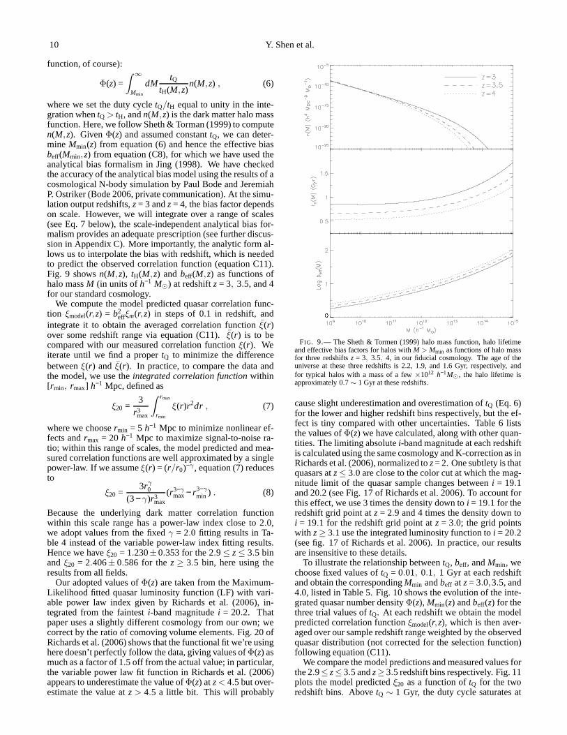
where we set the duty cycletQ/tH equal to unity in the inte-gration whentQ > tH, andn(M,z) is the dark matter halo massfunction. Here, we follow Sheth & Torman (1999) to computen(M,z). GivenΦ(z) and assumed constanttQ, we can deter-mine Mmin(z) from equation (6) and hence the effective biasbeff(Mmin,z) from equation (C8), for which we have used theanalytical bias formalism in Jing (1998). We have checkedthe accuracy of the analytical bias model using the results of acosmological N-body simulation by Paul Bode and JeremiahP. Ostriker (Bode 2006, private communication). At the simu-lation output redshifts,z= 3 andz= 4, the bias factor dependson scale. However, we will integrate over a range of scales(see Eq. 7 below), the scale-independent analytical bias for-malism provides an adequate prescription (see further discus-sion in Appendix C). More importantly, the analytic form al-lows us to interpolate the bias with redshift, which is neededto predict the observed correlation function (equation C11).Fig. 9 showsn(M,z), tH(M,z) and beff(M,z) as functions ofhalo massM (in units ofh−1 M⊙) at redshiftz= 3, 3.5, and 4for our standard cosmology.

We compute the model predicted quasar correlation func-tion ξmodel(r,z) = b2

effξm(r,z) in steps of 0.1 in redshift, andintegrate it to obtain the averaged correlation functionξ(r)over some redshift range via equation (C11).ξ(r) is to becompared with our measured correlation functionξ(r). Weiterate until we find a propertQ to minimize the differencebetweenξ(r) and ξ(r). In practice, to compare the data andthe model, we use theintegrated correlation functionwithin[rmin, rmax] h−1 Mpc, defined as

ξ20 =3

r3max

∫ rmax

rmin

ξ(r)r2dr , (7)

where we choosermin = 5 h−1 Mpc to minimize nonlinear ef-fects andrmax = 20 h−1 Mpc to maximize signal-to-noise ra-tio; within this range of scales, the model predicted and mea-sured correlation functions are well approximated by a singlepower-law. If we assumeξ(r) = (r/r0)−γ , equation (7) reducesto

ξ20 =3rγ

0

(3− γ)r3max

(r3−γmax− r3−γ

min ) . (8)

Because the underlying dark matter correlation functionwithin this scale range has a power-law index close to 2.0,we adopt values from the fixedγ = 2.0 fitting results in Ta-ble 4 instead of the variable power-law index fitting results.Hence we haveξ20 = 1.230±0.353 for the 2.9≤ z≤ 3.5 binand ξ20 = 2.406± 0.586 for thez≥ 3.5 bin, here using theresults from all fields.

Our adopted values ofΦ(z) are taken from the Maximum-Likelihood fitted quasar luminosity function (LF) with vari-able power law index given by Richards et al. (2006), in-tegrated from the faintesti-band magnitudei = 20.2. Thatpaper uses a slightly different cosmology from our own; wecorrect by the ratio of comoving volume elements. Fig. 20 ofRichards et al. (2006) shows that the functional fit we’re usinghere doesn’t perfectly follow the data, giving values ofΦ(z) asmuch as a factor of 1.5 off from the actual value; in particular,the variable power law fit function in Richards et al. (2006)appears to underestimate the value ofΦ(z) atz< 4.5 but over-estimate the value atz > 4.5 a little bit. This will probably

FIG. 9.— The Sheth & Tormen (1999) halo mass function, halo lifetimeand effective bias factors for halos withM > Mmin as functions of halo massfor three redshiftsz = 3, 3.5, 4, in our fiducial cosmology. The age of theuniverse at these three redshifts is 2.2, 1.9, and 1.6 Gyr, respectively, andfor typical halos with a mass of a few×1012 h−1M⊙, the halo lifetime isapproximately 0.7∼ 1 Gyr at these redshifts.

cause slight underestimation and overestimation oftQ (Eq. 6)for the lower and higher redshift bins respectively, but theef-fect is tiny compared with other uncertainties. Table 6 liststhe values ofΦ(z) we have calculated, along with other quan-tities. The limiting absolutei-band magnitude at each redshiftis calculated using the same cosmology and K-correction as inRichards et al. (2006), normalized toz= 2. One subtlety is thatquasars atz≤ 3.0 are close to the color cut at which the mag-nitude limit of the quasar sample changes betweeni = 19.1and 20.2 (see Fig. 17 of Richards et al. 2006). To account forthis effect, we use 3 times the density down toi = 19.1 for theredshift grid point atz= 2.9 and 4 times the density down toi = 19.1 for the redshift grid point atz = 3.0; the grid pointswith z≥ 3.1 use the integrated luminosity function toi = 20.2(see fig. 17 of Richards et al. 2006). In practice, our resultsare insensitive to these details.

To illustrate the relationship betweentQ, beff, andMmin, wechoose fixed values oftQ = 0.01, 0.1, 1 Gyr at each redshiftand obtain the correspondingMmin andbeff atz= 3.0,3.5, and4.0, listed in Table 5. Fig. 10 shows the evolution of the inte-grated quasar number densityΦ(z), Mmin(z) andbeff(z) for thethree trial values oftQ. At each redshift we obtain the modelpredicted correlation functionξmodel(r,z), which is then aver-aged over our sample redshift range weighted by the observedquasar distribution (not corrected for the selection function)following equation (C11).

We compare the model predictions and measured values forthe 2.9≤ z≤3.5 andz≥3.5 redshift bins respectively. Fig. 11plots the model predictedξ20 as a function oftQ for the tworedshift bins. AbovetQ ∼ 1 Gyr, the duty cycle saturates at

Quasar Correlation Function atz≥ 2.9 11

FIG. 10.— The top panel shows the integrated quasar luminosity function(LF) down to the magnitude cuti = 20.2, computed using the variable power-law fit function in Richards et al. (2006). The lower line segment shows theintegrated LF down toi = 19.1. The bottom two panels show the computedminimum halo masses and effective bias factors as functionsof redshift, forthe three trial values oftQ = 0.01, 0.1 and 1 Gyr. We have used the empiricalvalues ofΦ at the grid pointsz = 2.9, and 3.0 (i.e., three and four times thevalues down toi = 19.1, respectively), which causes the jump inMmin andbeffat these two redshift grid points, i.e., we are targeting more luminous quasarsatz= 2.9, 3.0. The slight kink aroundz= 4.5 in all three panels is due to theK-correction (see figure 17 of Richards et al. 2006).

TABLE 5TRIAL VALUES OF tQ AT REDSHIFTz= 3.0, 3.5, 4.0 AND THE

CORRESPONDINGMmin AND beff , ASSUMING THE FIDUCIAL ΛCDMCOSMOLOGY.

z Φ (h3 Mpc−3) tQ (Gyr) Mmin (h−1M⊙) beff

3.0 5.591×10−7 0.01 2.33×1012 7.60.1 6.10×1012 9.81 1.32×1013 12.3

3.5 3.251×10−7 0.01 2.09×1012 9.00.1 4.98×1012 11.41 9.76×1012 13.9

4.0 1.009×10−7 0.01 2.29×1012 11.10.1 4.87×1012 13.71 8.41×1012 16.0

unity, and the predicted correlation function flattens. Thehor-izontal lines show the values and 1σ errors ofξ20 computedusing our fixed power-law fits, for the two redshift bins re-spectively. For the 2.9 ≤ z≤ 3.5 bin, the estimated quasarlifetime is tQ ∼ 15 Myr with lower limit 3.6 Myr and upperlimit 47 Myr for the 1-σ error of the measuredξ20. For thez≥ 3.5 redshift bin, the estimated quasar lifetime istQ ∼ 160Myr with lower limit ∼ 30 Myr and upper limit∼ 600 Myrfor the 1-σ error of the measuredξ20. To phrase this in terms

FIG. 11.— Comparison of the measured and model predicted clusteringstrengthξ20, defined in equation (7). Solid lines correspond to the 2.9 ≤z≤ 3.5 bin and dashed lines correspond to thez≥ 3.5 bin. The thick andlight horizontal lines show the measured clustering strength and 1−σ errors.The match of the model predictedξ20 (blue lines for the fiducialσ8 = 0.751and red lines forσ8 = 0.84) with the measuredξ20 gives the average quasarlifetime tQ within that redshift bin. The uncertainty in measuredξ20 gives alarge uncertainty intQ. Quasars in the higher redshift bin have largertQ onaverage. The fiducial values oftQ inferred from this figure (theσ8 = 0.751case) are:tQ = 15 Myr for 2.9≤ z≤ 3.5 andtQ = 160 Myr forz≥ 3.5.

of the duty cycle, we take the average halo lifetime to be 1Gyr at these redshifts (see Fig. 9). Therefore the duty cycleis0.004∼ 0.05 for the lower redshift bin and 0.03∼ 0.6 for thehigher redshift bin.

In the model we are using,tQ is very sensitive to the cluster-ing strength, as shown in Fig. 11. A small change in the mea-sured quasar correlation function will result in a substantialchange intQ. Using different fitting results for the measuredξ20 (e.g., those for good fields only) will certainly change thevalue oftQ. However, the formal 1−σ errors oftQ are largeenough to encompass these changes. The model is also sen-sitive to the adopted value ofσ8, whose consensus value haschanged significantly since the release of the WMAP3 data(Spergel et al. 2006). By increasingσ8 we can increase themodel predictedξ20 given the sametQ18. The results for theWMAP first year valueσ8 = 0.84 (Spergel et al. 2003) are alsoplotted in Fig. 11 as red lines. In this case thetQ values areslightly lower for the two redshift bins, but are still within the1-σ errors of the fiducialσ8 case. Combining these effects,we conclude that this approach can only constrain the quasarlifetime within a very broad range of 106−108 yr, which is, ofcourse, consistent with many other approaches (e.g., Martini2004 and references therein). On the other hand, our resultsdo show, on average, a largertQ and duty cycle for the higherredshift bin.

There are other assumptions in our model that we shouldconsider. In particular, there is the possibility that quasarscluster more than their dark matter halos due to physical ef-

18 The ξ20 result is insensitive to other cosmological parameters such asΩM.

12 Y. Shen et al.

TABLE 6QUASAR SPACE DENSITY, Mmin AND beff AT EACH REDSHIFT GRID

z Mi,limit Φ′(Mi < Mi,limit ) Φ nQSO D(z) Mmin beff

(z= 2) h3 Mpc−3 h3 Mpc−3 h3 Mpc−3 h−1 M⊙

2.9 – 4.533×10−7 5.268×10−7 1.820×10−7 0.3375 3.11×1012 7.82.9∗ -26.42 1.092×10−6 1.268×10−6 – – – –2.9∗∗ -27.52 1.511×10−7 1.756×10−7 – – – –3.0 – 4.808×10−7 5.592×10−7 2.642×10−7 0.3293 2.81×1012 8.03.0∗ -26.51 8.445×10−7 9.821×10−7 – – – –3.0∗∗ -27.61 1.202×10−7 1.398×10−7 – – – –3.1 -26.59 6.722×10−7 7.826×10−7 2.735×10−7 0.3214 2.26×1012 7.93.2 -26.66 5.345×10−7 6.228×10−7 3.102×10−7 0.3139 2.33×1012 8.33.3 -26.74 4.156×10−7 4.847×10−7 2.369×10−7 0.3068 2.43×1012 8.73.4 -26.82 3.272×10−7 3.820×10−7 1.551×10−7 0.3000 2.49×1012 9.13.5 -26.84 2.783×10−7 3.251×10−7 1.254×10−7 0.2934 2.48×1012 9.4

3.5 -26.84 2.783×10−7 3.251×10−7 1.254×10−7 0.2934 5.76×1012 11.93.6 -26.88 2.283×10−7 2.670×10−7 1.406×10−7 0.2871 5.66×1012 12.33.7 -26.96 1.774×10−7 2.076×10−7 1.462×10−7 0.2811 5.66×1012 12.83.8 -27.04 1.377×10−7 1.612×10−7 1.453×10−7 0.2753 5.64×1012 13.33.9 -27.12 1.070×10−7 1.254×10−7 9.720×10−8 0.2698 5.62×1012 13.74.0 -27.17 8.608×10−8 1.009×10−7 7.656×10−8 0.2644 5.53×1012 14.24.1 -27.24 6.821×10−8 8.002×10−8 6.413×10−8 0.2593 5.46×1012 14.74.2 -27.32 5.389×10−8 6.326×10−8 5.147×10−8 0.2544 5.39×1012 15.14.3 -27.41 4.171×10−8 4.898×10−8 4.322×10−8 0.2496 5.34×1012 15.64.4 -27.49 3.253×10−8 3.823×10−8 2.950×10−8 0.2450 5.28×1012 16.14.5 -27.53 2.763×10−8 3.248×10−8 3.040×10−8 0.2406 5.10×1012 16.54.6 -27.50 2.566×10−8 3.018×10−8 2.590×10−8 0.2364 4.81×1012 16.74.7 -27.45 2.437×10−8 2.867×10−8 2.435×10−8 0.2323 4.51×1012 17.04.8 -27.46 2.154×10−8 2.535×10−8 1.846×10−8 0.2283 4.31×1012 17.34.9 -27.54 1.754×10−8 2.066×10−8 1.492×10−8 0.2245 4.21×1012 17.75.0 -27.64 1.411×10−8 1.662×10−8 7.542×10−9 0.2207 4.12×1012 18.25.1 -27.74 1.136×10−8 1.339×10−8 3.177×10−9 0.2171 4.03×1012 18.65.2 -27.85 9.163×10−9 1.080×10−8 3.853×10−9 0.2137 3.93×1012 19.15.3 -27.95 7.502×10−9 8.847×10−9 3.895×10−9 0.2103 3.83×1012 19.5

NOTE. — Mi,limit is the i band limiting absolute magnitude, K-corrected toz = 2. Φ′ is the integrated quasar number density over the apparent magnitude

range, in the same cosmology as in Richards et al. (2006), converted usingh = 0.7 to units ofh3 Mpc−3. Φ is the corresponding quasar number density in ourcosmology, converted usingh = 0.71 toh3 Mpc−3. There are three entries for each of thez= 2.9 andz= 3.0 grids, corresponding to a magnitude limit ofi = 20.2(one asterisk),i = 19.1 (two asterisks), and using the empirical values we adoptedat these two redshift grids (see text; no asterisks). The apparenti-band limitingmagnitude cut isi = 20.2 for z≥ 3.1. nQSO is the observed overall quasar number density for all fields,in the current cosmology; the difference betweennQSOandΦ reflects the selection function and difference between the fitted power-law function and binned luminosity function.D(z) is the linear growth factor. Alsotabulated are the corresponding minimal halo massMmin and effective bias factorsbeff at each redshift grid, computed using the fiducial values oftQ, i.e.,tQ = 15Myr for 2.9≤ z≤ 3.5 andtQ = 160 Myr forz≥ 3.5.

fects that modulate the formation of quasars on very largescales. For example, the process of reionization may showlarge spatial modulation, which might affect the number den-sity of young galaxies and quasars on large scales (e.g.,Babich & Loeb 2006). We have also assumed that each halohosts only one luminous quasar. However, Hennawi et al.(2006a) show that quasars (at lower redshift) are very stronglyclustered on small scales, with some close binaries clearlyina single halo. Searches for multiple quasars at higher red-shift have also been successful (Hennawi et al., in prepara-tion), suggesting that at high redshift as well, a single halocan host more than one quasar.

Table 6 uses the fiducial values oftQ we derived for theσ = 0.751 case to estimate the minimal halo mass and biasfactors of high redshift quasars, but the values ofMmin andbeffdepend only weakly ontQ, as one can see from Table 5. Thevalues ofMmin andbeff are tabulated in Table 6, for each of theredshift bins. Note that the change ofMmin within each red-shift bin may not be real because we have assumed constanttQthroughout the redshift bin. On the other hand, the host halosfor the higher redshift bin have, on average, a larger minimalhalo mass of∼ 4−6×1012 M⊙ than that for the lower redshift

bin of ∼ 2− 3×1012 M⊙. This is expected, because quasarsin the higher redshift bin have higher mean luminosity andhence should reside in more massive halos. From Table 6 itis clear that high redshift quasars are strongly biased objects,and the effective bias factor increases with redshift.

4. SUMMARY AND CONCLUSIONS

We have used∼ 4000 high redshift SDSS quasars to mea-sure the quasar correlation function atz ≥ 2.9. The clus-tering of these high redshift quasars is stronger than thatof their low redshift counterparts. Over the range of 4<rp < 150 h−1 Mpc, the real-space correlation function is fit-ted by a power-law formξ(r) = (r/r0)−γ with r0 ∼ 15 h−1

Mpc andγ ∼ 2. When we divide the clustering ample intotwo broad redshift bins, 2.9 ≤ z≤ 3.5 andz≥ 3.5, we findthat the quasars in the higher redshift bin show substantiallystronger clustering properties, with a comoving correlationlength r0 = 24.3± 2.4 h−1 Mpc assuming a fixed power-lawindex γ = 2.0. The lower redshift bin has a comoving cor-relation lengthr0 = 16.9± 1.7 h−1 Mpc, assuming the samepower-law index.

We followed Martini & Weinberg (2001) to relate this

Quasar Correlation Function atz≥ 2.9 13

strong clustering signal to the quasar luminosity function(Richards et al. 2006), the quasar lifetime and duty cycle,and the mass function of massive halos. We find the mini-mum massMmin of halos in which luminous quasars in oursample reside, as well as the clustering bias factor for thesehalos. High redshift quasars are highly biased objects withrespect to the underlying matter, while the minimal halo massshows no strong evolution with redshift for our flux-limitedsample. Quasars with 2.9≤ z≤ 3.5 reside in halos with typ-ical mass∼ 2− 3×1012 h−1 M⊙; quasars withz≥ 3.5 residein halos with typical mass∼ 4− 6×1012 h−1 M⊙. The slightdifference ofMmin in the two redshift bins is expected becausequasars in the higher redshift bin have mean luminosity thatisapproximately two times that of quasars in the lower redshiftbin, and should reside in more massive halos. We further esti-mated the quasar lifetimetQ. We get atQ value of 4∼ 50 Myrfor the 2.9 ≤ z≤ 3.5 bin and 30∼ 600 Myr for thez≥ 3.5bin; which is broadly consistent with the quasar lifetime of106 −108 yr estimated from other methods (e.g., Martini 2004and references therein). This corresponds to a duty cycle of0.004∼ 0.05 for the lower redshift bin and 0.03∼ 0.6 for thehigher redshift bin, where we take the average halo lifetimeto be 1 Gyr. In general we find the average lifetime is higherfor the higher redshift bin, which could either be due to theredshift evolution or an effect of the luminosity dependenceof tQ. However, we emphasize that our approach is subject toa variety of uncertainties, including errors in the clusteringmeasurements themselves, uncertainties inσ8 and the halomass function, and the validity of the assumptions we haveadopted.

It is interesting to note that recentChandra and XMM-Newtonstudies on the clustering of X-ray selected AGN haverevealed a larger correlation length than optical AGN. In par-ticular, hard X-ray AGN have a correlation lengthr0 ∼ 15h−1

Mpc at z . 2 (e.g., Basilakos et al. 2004; Gilli et al. 2005;Puccetti et al. 2006; Plionis 2006). Given the fact that X-ray selected AGN have considerably lower mean bolometricluminosity than do optically-selected AGN (e.g., Mushotzky2004), this implies, once again, that the instantaneous lumi-nosity is not a reliable indicator of the host halo mass at thelow luminosity end (e.g., Hopkins et al. 2005). Shen et al.(2007) have suggested an evolutionary model of AGN accre-tion in which an AGN evolves from being dominant in theoptical to dominant in X-rays when the accretion rate drops.Hence those strongly clustering hard X-ray AGN were proba-bly once very luminous quasars in the past with high peak lu-minosities. When they dim and turn into hard X-ray sources,their spatial clustering strength remains. However, the cur-rent X-ray AGN sample is still very limited compared withoptically selected samples, hence the uncertainty in the X-rayAGN correlation length is large.

The work described in this paper can be extended in a va-riety of ways. Our sample cannot explore clustering below∼ 1 h−1 Mpc because of fiber collisions; we are extendingthe methods of Hennawi et al. (2006a) to find close pairs ofhigh-redshift quasars, to determine whether the excess clus-tering found at moderate redshift extends toz > 3. Extend-ing the clustering analysis to lower luminosities will be im-portant, given theoretical predictions of a strong luminositydependence to the clustering signal at high redshifts (Hop-kins et al. 2006). The repeat scans of the Southern EquatorialStripe in SDSS (Adelman-McCarthy et al. 2007) will allowus to extend the luminosity range of our sample, and redshiftsof the fainter quasars are already being obtained (Jiang et al.

2006). The massive halos that we predict host the luminousquasars must also contain a substantial number of ordinarygalaxies, and we plan deep imaging surveys of high-redshiftquasar fields to measure the quasar-galaxy crosss-correlationfunction (see Stiavelli et al. 2005; Ajiki et al. 2006). Finally,more work is needed on simulations of quasar clustering. Ourquasar lifetime/duty cycle calculation is frustratingly impre-cise, and further explorations of the behavior of highly biasedrare halos at high redshifts may yield ways to constrain dutycycles more directly from the data, and understand the uncer-tainties of the technique in more detail.

Finally, we need to make more detailed comparisons ofhigh-redshift quasar clustering with that of luminous galax-ies at the same redshift. The duty cycle of quasars at theseredshifts is a few percent at most, thus there is a populationof galaxies with quiescent central black holes that is just asstrongly clustered. The correlation length of Lyman-breakgalaxies at these redshifts is∼ 5h−1Mpc (Adelberger et al.2005a), but the clustering strength appears to increase (albeitat z∼ 2) with increasing observed K-band luminosity (Adel-berger et al. 2005b; Allen et al. 2005) and/or color (Quadriet al. 2006). The duty cycle we have calculated should agreewith the ratio of number densities of luminous quasars, andthat of the parent host galaxy population. The challenge willbe to identify this parent population unambigously.

We thank Paul Bode and J. P. Ostriker for useful discussionsand for providing us their numerical simulation results used inAppendix C, and Jim Gray for his work on the CAS. YS andMAS acknowledge the support of NSF grant AST-0307409.

Funding for the SDSS and SDSS-II has been provided bythe Alfred P. Sloan Foundation, the Participating Institutions,the National Science Foundation, the U.S. Department of En-ergy, the National Aeronautics and Space Administration, theJapanese Monbukagakusho, the Max Planck Society, and theHigher Education Funding Council for England. The SDSSWeb Site is http://www.sdss.org/.

The SDSS is managed by the Astrophysical Research Con-sortium for the Participating Institutions. The ParticipatingInstitutions are the American Museum of Natural History, As-trophysical Institute Potsdam, University of Basel, Univer-sity of Cambridge, Case Western Reserve University, Uni-versity of Chicago, Drexel University, Fermilab, the Institutefor Advanced Study, the Japan Participation Group, JohnsHopkins University, the Joint Institute for Nuclear Astro-physics, the Kavli Institute for Particle Astrophysics andCos-mology, the Korean Scientist Group, the Chinese Academyof Sciences (LAMOST), Los Alamos National Laboratory,the Max-Planck-Institute for Astronomy (MPIA), the Max-Planck-Institute for Astrophysics (MPA), New Mexico StateUniversity, Ohio State University, University of Pittsburgh,University of Portsmouth, Princeton University, the UnitedStates Naval Observatory, and the University of Washington.

Facilities: Sloan

14 Y. Shen et al.

REFERENCES

Abazajian, K., et al. 2003, AJ, 126, 2081Abazajian, K., et al. 2005, AJ, 129, 1755Adelberger, K. L., et al. 1998, ApJ, 505, 18Adelberger, K. L., Steidel, C. C., Pettini, M., Shapley, A. E., Reddy, N. A., &

Erb, D. K. 2005a, ApJ, 619, 697Adelberger, K. L., Erb, D.K., Steidel, C. C.,Reddy, N. A., Pettini, M., &

Shapley, A. E. 2005b, ApJ, 620, L75Adelman-McCarthy, J. K., et al. 2006, ApJS, 162, 38Adelman-McCarthy, J. K., et al. 2007, ApJS, submittedAjiki, M. et al. 2006, PASJ, 58, 499Allen, P. D., Moustakas, L. A., Dalton, G., MacDonald, E., Blake, C.,

Clewley, L., Heymans, C., and Wegner, G. 2005, MNRAS, 360, 1244Anderson, S. F., et al. 2003, AJ, 126, 2209Babich, D., & Loeb, A. 2006, ApJ, 640, 1Bardeen, J., Bond, J. R., Kaiser, N. & Szalay, A. S. 1986, ApJ,304, 15Basilakos, S., Georgakakis, A., Plionis, M., & Georantopoulos, I. 2004, ApJ,

607, L79Blanton, M. R., et al. 2000, ApJ, 531, 1Blanton, M. R., et al. 2003, AJ, 125, 2276Blanton, M. R., et al. 2005, AJ, 129, 2562Bode, P., & Ostriker, J.P. 2003, ApJS, 145, 1Bode, P., Ostriker, J.P., & Xu, G. 2000, ApJS, 128, 561Cohen, J. G., et al. 1996, ApJ, 471, 5Colless, M., et al. 2001, MNRAS, 328, 1039Connolly, A. J. et al. 2006, in preparationCroom, S. M., & Shanks, T. 1996, MNRAS, 281, 893Croom, S. M., et al. 2004, MNRAS, 349, 1379Croom, S. M., et al. 2005, MNRAS, 356, 415da Ângela, J. et al. 2005, MNRAS, 360, 1040Davis, M., & Peebles, P. J. E. 1983, ApJ, 267, 465Djorgovski, S. 1991, ASPC, 21, 349Djorgovski, S. G., Stern, D., Mahabal, A. S., & Brunner, R. 2003, ApJ, 596,

1Eisenstein, D. J. et al. 2005, ApJ, 633, 560Fan, X. 1999, AJ, 117, 2528Fan, X., et al. 2001, AJ, 122, 2833Ferrarese, L. 2002, ApJ, 578, 90Fukugita, M., et al. 1996, AJ, 111, 1748Gaskell, C. M. 1982, ApJ, 263, 79Giavalisco, M., et al. 1998, ApJ, 503, 543Gilli, R., et al. 2005, A&A, 430, 811Groth, E. J., & Peebles, P. J. E. 1977, ApJ, 217, 385Gunn, J. E., et al. 1998, AJ, 116, 3040Gunn, J. E., et al. 2006, AJ, 131, 2332Haiman, Z., & Hui, L. 2001, ApJ, 547, 27Hamilton, A. J. S. 1993, ApJ, 417, 19Hamilton, A. J. S., & Tegmark, M. 2004, MNRAS, 349, 115Hawkins, E., et al. 2003, MNRAS, 346, 78Heitmann, K., Lukic, Z., Habib, S., & Ricker, P. M. 2006, ApJ,642, L85Hennawi, J., et al. 2006a, AJ, 131, 1Hennawi, J., et al. 2006b, ApJ, 651, 61Hogg, D. W. 1999, astro-ph/9905116Hogg, D. W., Finkbeiner, D. P., Schlegel, D. J., & Gunn, J. E. 2001, AJ, 122,

2129Hopkins, P. F., Hernquist, L., Martini, P., Cox, J., Robertson, B., Di Matteo,

T., & Springel, V. 2005, ApJ, 625, L71Hopkins, P. F. et al. 2006, in preparationIovino, A., & Shaver, P. A. 1988, ApJ, 330, L13Ivezic, Z., et al. 2004, AN, 325, 583Jenkins, A., et al. 2001, MNRAS, 321, 372Jiang, L. et al. 2006, AJ, 131, 2788Jing, Y. P. 1998, ApJ, 503, L9Kaiser, N. 1984, ApJ, 284, L9Kaiser, N. 1986, MNRAS, 219, 785Kaiser, N. 1987, MNRAS, 227, 1Kashikawa, N., et al. 2006, ApJ, 637, 631Kollmeier, J. A. et al. 2006, ApJ, 648, 128Kormendy, J., & Richstone, D. 1995, ARA&A, 33, 581Kundic, T. 1997, ApJ, 482, 631La Franca, F., Andreani, P., & Cristiani, S. 1998, ApJ, 497, 529Lacey, C., & Cole, S. 1993, MNRAS, 262, 627Landy, S. D., & Szalay, A. S. 1993, ApJ, 412, 64

Lee, K.-S., et al. 2006, ApJ, 642, 63Lidz, A., Hopkins, P. F., Cox, T. J., Hernquist, L., & Robertson, B. 2006, ApJ,

641, 41Lupton, R., Gunn, J. E., Ivezic, Z., Knapp, G. R., & Kent, S. 2001, ASP

Conference Proceedings, 238, 269Lynden-Bell, D. 1969, Nature, 223, 690Magorrian, J., et al. 1998, AJ, 115, 2285Martini, P. 2004, in Ho L. C., ed., Coevolution of Black Holesand Galaxies.

Cambridge Univ. Press, Cambridge, p. 406Martini, P., & Weinberg, D. H. 2001, ApJ, 547, 12Meneux, B., et al. 2006, A&A, 452, 387Myers, A. D., et al. 2006a, ApJ, 638, 622Myers, A. D., et al. 2006b, submittedMyers, A. D., et al. 2006c, submittedNavarro, J. F., Frenk, C. S., & White, S. D. M. 1997, ApJ, 490, 493Osmer, P. S. 1981, ApJ, 247, 762Ouchi, M., et al. 2005, ApJ, 635, L117Padmanabhan, N. et al. 2007, in preparationPercival, W., et al. 2006, submitted, astro-ph/0608636Pier, J. R., et al. 2003, AJ, 125, 1559Plionis, M. 2006, proceedings of the XXVIth Astrophysics Moriond Meeting,

eds. L.Tresse, S. Maurogordato and J. Tran Thanh Van, astro-ph/0607324Porciani, C., Magliocchetti, M., & Norberg, P. 2004, MNRAS,355, 1010

(PMN04)Porciani, C., Norberg, P. 2006, MNRAS, 371, 1824Press, W. H., & Schechter, P. 1974, ApJ, 187, 425Puccetti, S., et al. 2006, A&A, 457, 501Quadri, R., et al. 2006, astro-ph/0606330Richards, G. T., et al. 2002a, AJ, 124, 1Richards, G. T., et al. 2002b, AJ, 123, 2945Richards, G. T., et al. 2006, AJ, 131, 2766Roukema, B. F., Mamon, G. A., & Bajtlik, S. 2002, A&A, 382, 397Salpeter, E. E. 1964, ApJ, 140, 796Schlegel, D. J., Finkbeiner, D. P., & Davis, M. 1998, ApJ, 500, 525Schneider, D. P., Schmidt, M., & Gunn, J. E. 1994, AJ, 107, 1245Schneider, D. P., et al. 2000, AJ, 120, 2183Schneider, D. P., et al. 2005, AJ, 130, 367Schneider, D. P., et al. 2006, submittedScranton, R., et al. 2005, ApJ, 633, 589Serber, W., Bahcall, N., Ménard, B., & Richards, G. 2006, ApJ, 643, 68Shaver, P. A. 1984, A&A, 136, L9Shen, Y., et al. 2007, ApJ, 654, L115, astro-ph/0611635Sheth, R. K., & Tormen, G. 1999, MNRAS, 308, 119Smith, J. A., et al. 2002, AJ, 123, 2121Spergel, D. N., et al. 2003, ApJS, 148, 175Spergel, D. N., et al. 2006, astro-ph/0603449Steidel, C. C., et al. 1998, ApJ, 492, 428Stephens, A. W., Schneider, D. P., Schmidt, M., Gunn, J. E., &Weinberg, D.

H. 1997, AJ, 114, 41Stiavelli, M. et al. 2005, ApJ, 622, L1Stoughton, C., et al. 2002, AJ, 123, 485SubbaRao, M., Frieman, J., Bernardi, M., Loveday, J., Nichol, B., Castander,

F., & Meiksin, A. 2002, SPIE, 4847, 452Sugiyama, N. 1995, ApJS, 100, 281Tegmark, M., & Peebles, P. J. E. 1998, ApJ, 500, 79Tegmark, M., et al. 2004, ApJ, 606, 702Tegmark, M., et al. 2006, PRD, 74, 123507Totsuji, H., & Kihara, T. 1969, PASJ, 21, 221Tremaine, S., et al. 2002, ApJ, 574, 740Tucker, D. L., et al. 2006, AN, 327, 821Tytler, D., & Fan, X. 1992, ApJS, 79, 1Vanden Berk, D. E., et al. 2001, AJ, 122, 549Weinberg, D. H., Davé, R., Katz, N., & Hernquist, L. 2004, ApJ, 601, 1Weymann, R. J., Morris, S. L., Foltz, C. B., & Hewett, P. C. 1991, ApJ, 373,

23York, D. G., et al. 2000, AJ, 120, 1579Yu, Q., & Tremaine, S. 2002, MNRAS, 335, 965Zehavi, I., et al. 2004, ApJ, 608, 16Zehavi, I., et al. 2005, ApJ, 630, 1

Quasar Correlation Function atz≥ 2.9 15

TABLE 7EMISSION LINE SHIFTS

Lyα - SiIV Lyα-CIV SiIV - MgII CIV - MgII CIII] - MgII MgII - [OIII]

mean vel shift (km s−1) -463 -1478 61 921 827 -97σ (km s−1) 1178 1217 744 746 604 269

y = ax+ b a b(km s−1) σ (km s−1)CIV - MgII vs. SiIV - CIV -0.5035 486.7 660CIV - MgII vs. CIII] - CIV -0.8024 845.8 594SiIV - MgII vs. SiIV - CIII] 0.6958 596.5 569

NOTE. — The MgII - [OIII] (i.e., systemic) lineshift and 1σ error are taken from Richards et al. (2002). Positive valuesindicate a blueshift.The dispersion of the shift between CIV and MgII is somewhat larger than the value of 511 km s−1 quoted by Richards et al. (2002), but is consistent with theirrecent result using a much larger sample from SDSS DR4 (∼ 770 km s−1).

APPENDIX

A. QUASAR REDSHIFT DETERMINATION

A.1 Broad Emission Line Shifts

High redshift quasars (z≥ 2.9) have only a few strong emission lines that fall within the SDSS spectral coverage (3800-9200Å): Lyα (1216 Å), SiIV/OIV (1397 Å), CIV (1549 Å) and CIII] (1909 Å). The Lyα emission line is heavily affected by the Lymanα forest, and is blended with NV 1240 Å. In addition, high-ionization broad emission lines such as CIV are blueshifted by severalhundred km s−1 from the redshift determined from narrow forbidden lines like [OIII]5007 Å (e.g., Gaskell 1982; Tytler & Fan1992; Richards et al. 2002a). We could simply correct the redshift derived from each observed line for the (known) mean offset ofthat line from systemic (e.g., Vanden Berk et al. 2001; Richards et al. 2002a). We can do better than this, however, by examiningthe relationships between the shifts of different lines.

To understand these relationships, we use a sample of quasars drawn from the SDSS DR3 quasar catalog (Schneider et al.2005) with 1.8≤ z≤ 2.2; for these objects, the lines SiIV, CIV, CIII] and MgII2800 Å all fall in the SDSS spectral coverage. TheMgII line has a small and known offset from the systemic redshift (Richards et al. 2002a), thus tying our results to MgII allowsus to determine the systemic redshift for each object. We exclude from the sample those objects which show evidence for a broadabsorption line, determined using the “balnicity” index (BI) of Weymann et al. (1991) and using the Vanden Berk et al. (2001)quasar composite spectrum to define the continuum level.

We fit a log-normal to each of the four lines (with a second log-normal added for the neighboring lines HeII1640 Å andAl III1857 Å), together with the local continuum. The centroid foreach line is determined following Hennawi et al. (2006b): wecalculate the mode of the pixels within±1.5σ of the fitted Gaussian line center using 3×median− 2×mean. We include in themode calculation those pixels with flux:

fλ >0.6Ai√2πσi

+Cλ +∑

j 6=i

A j√

2πσ je−(log10λ−log10λ j )

2/2σ2j , (A1)

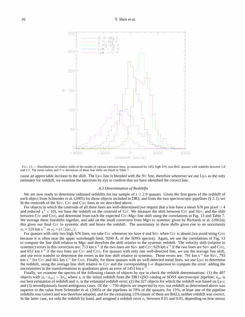
whereAi , log10λi andσi are the amplitude, central wavelength, and dispersion of the best fit log-normal to theith emission lineandCλ is the linear continuum. Lines with a signal-to-noise ratio(S/N) less than 6 per pixel, or with log-normal fits withχ2 > 5are rejected from further consideration. This gives us a sample of 1652 quasars with robust line measurements. Fig. 12 shows thedistribution of shifts between various lines. The means andstandard deviations of these distributions are given in Table 7. Thecontribution from the line fitting error is negligible compared to the “intrinsic” dispersion of velocity shifts.

These line shifts are correlated with each other, as Fig. 13 shows. In each panel, we show the best-fit line to the correlations,giving each point equal weight. Given these correlations, we can use the shifts between the lines we observe at high redshift todetermine the offset to MgII, and thus to the systemic redshift.

There are also correlations between the lineshifts and quantities such as the quasar luminosity, color, line width, andequivalentwidth. However, these correlations show large scatter, andare therefore not as good for determining the true redshiftsof thequasars.

A.2 Lyα − SiIV, Ly α − CIV Line Shifts

The CIV line lies beyond the SDSS spectra forz> 4.9. In addition, some quasars have weak metal emission lines,which are oftoo low S/N to allow us to measure a redshift from them. In these cases, we will measure the redshift from the Lyα line. In orderto understand the biases that this gives, we selected a sample of 1114 non-BAL quasars with 2.9 < z< 4.8 with high S/N SiIVand CIV lines. The center of the Lyα line was taken to be the wavelength of maximum flux. To reduce the effects of fluctuationsand strong skylines, we mask out 5-σ outliers from the 20-pixel smoothed spectrum and the 5577 Å skyline region (about 20pixels), and smooth the spectrum by 15 pixels before identifying the peak pixel; all spectra were examined by eye to confirm thatwe correctly identified the peak of Lyα.

Fig. 14 shows the shifts between Lyα and the CIV and SiIV lines as a function of redshift. The mean shift is∼ 500 km s−1, witha 1σ scatter of 1200 km s−1 for Lyα-SiIV; and is∼ 1500 km s−1, with a 1σ scatter of 1200 km s−1 for Lyα-CIV. This systematicoffset is caused by absorption blueward of the Lyα forest; over this redshift range, the increasing strength of the forest doesn’t

16 Y. Shen et al.

FIG. 12.— Distributions of relative shifts of the modes of various emission lines, as measured for 1652 high S/N, non-BAL quasars with redshifts between 1.8and 2.2. The mean values and 1−σ deviations of these line shifts are listed in Table 7.

cause an appreciable increase in the shift. The Lyα line is blended with the NV line, therefore whenever we use Lyα as the onlyestimator for redshift, we examine the spectrum by eye to confirm that we have identified the correct line.

A.3 Determination of Redshifts

We are now ready to determine unbiased redshifts for our sample of z≥ 2.9 quasars. Given the first guess of the redshift ofeach object from Schneider et al. (2005) for those objects included in DR3, and from the two spectroscopic pipelines (§ 2.1), wefit the centroids of the SiIV, CIV and CIII] lines as we described above.

For objects in which the centroids of all three lines are well-determined (we require that a line have a mean S/N per pixel> 4and reducedχ2 < 10), we base the redshift on the centroid of CIV. We measure the shift between CIV and SiIV, and the shiftbetween CIV and CIII], and determine from each the expected CIV-MgII line shift using the correlations in Fig. 13 and Table 7.We average these lineshifts together, and add on the small correction from MgII to systemic given by Richards et al. (2002a);this gives our final CIV to systemic shift and hence the redshift. The uncertainty inthese shifts gives rise to an uncertaintyσv = 519 km s−1 or σz = (1+ z)σv/c.

For quasars with only two high S/N lines, we take CIV whenever we have it and SiIV when CIV is absent (we avoid using CIII]because it is often near the upper wavelength limit, 9200 Å, of the SDSS spectra). Again, we use the correlations of Fig. 13to compute the line shift relative to MgII and therefore the shift relative to the systemic redshift. The velocity shift (relative tosystemic) errors in this correction are: 713 km s−1 if the two lines are SiIV and CIV; 629 km s−1 if the two lines are SiIV and CIII],and 652 km s−1 if the two lines are CIV and CIII]. For quasars with only one well-detected line, we use the average line shift,and use error transfer to determine the errors in the line shift relative to systemic. These errors are: 791 km s−1 for SiIV, 793km s−1 for CIV and 661 km s−1 for CIII]. Finally, for those quasars with no well-detected metal lines, we use Lyα to determinethe redshift, using the average line shift relative to CIV and the corresponding 1-σ dispersion to compute the error: adding theuncertainties in the transformations in quadrature gives an error of 1453 km s−1.

Finally, we examine the spectra of the following classes of objects by eye to check the redshift determinations: (1) the 407objects with|zi − zsys| > 3σz, wherezi is the initial redshift from the DR3 QSO catalog or SDSS spectroscopic pipeline;zsys isour best estimation of redshift andσz is the estimated redshift error; (2) the 327 objects for which the redshift was based on Lyα;and (3) serendipitously found ambiguous cases. Of the∼ 750 objects we inspected by eye, our redshift as determined above wassuperior to the value from Schneider et al. (2005) or the pipelines in 70% of the quasars; for 15%, at least one of the pipelineredshifts was correct and was therefore adopted, and for theremaining 15% (many of them are BAL), neither redshift was correct.In the latter case, we refit the redshift by hand, and assigneda redshift errorσz between 0.01 and 0.05, depending on how messy

Quasar Correlation Function atz≥ 2.9 17

−4000 −3000 −2000 −1000 0 1000 2000−3000

−2000

−1000

0

1000

2000

3000

4000

5000

SiIV − CIV shift (km/s)

CIV

− M

gII s

hift

(km

/s)

−3000 −2000 −1000 0 1000 2000 3000−3000

−2000

−1000

0

1000

2000

3000

4000

5000

CIII] − CIV shift (km/s)

CIV

− M

gII s

hift

(km

/s)

−5000 −4000 −3000 −2000 −1000 0 1000 2000 3000−4000

−3000

−2000

−1000

0

1000

2000

3000

4000

SiIV − CIII] shift (km/s)

SiIV

− M

gII s

hift

(km

/s)

FIG. 13.— Correlations between various emission line shifts. Blue dots are data points and red lines are fitted linear functions. These correlations are used inour redshift estimation. The fitted linear parameters and 1−σ deviations are listed in Table 7.

3 3.2 3.4 3.6 3.8 4 4.2 4.4 4.6

−4000

−3000

−2000

−1000

0

1000

2000

3000

4000

zSi IV

Lyα

− S

i IV

shi

ft (k

m/s

)

3 3.2 3.4 3.6 3.8 4 4.2 4.4 4.6−6000

−5000

−4000

−3000

−2000

−1000

0

1000

2000

3000

zC IV

Lyα

− C

IV s

hift

(km

/s)

FIG. 14.— Relative shifts of Lyα versus SiIV and CIV emission lines as a function of redshift. Red lines indicatethe mean value of line shifts. The meanvalues of line shifts and 1−σ deviations are listed in Table 7.

the spectrum was. There were 29 objects whose redshifts wereundetermined, lay below 2.9, or were simply not quasars. Thusthe parent sample, from which we will construct our clustering subsample, contains 6,109 objects (including∼ 200 duplicates).

Finally, we compared the redshifts in our sample with the separately compiled DR5 quasar sample of Schneider et al. (2006).The difference in redshifts follows a Gaussian distribution with zero mean and a dispersion of 0.01, comparable to our estimatederrors.

B. SURVEY GEOMETRY

SDSS spectroscopic targets are selected from the imaging data, and thus the spectroscopic footprint is a complicated combi-nation of the individual runs which make up the imaging data,and the circular 1.49 radius tiles on which spectroscopic targets

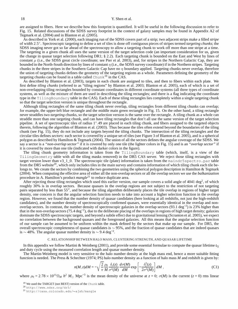
18 Y. Shen et al.

are assigned to fibers. Here we describe how this footprint isquantified. It will be useful in the following discussion to refer toFig. 15. Related discussions of the SDSS survey footprint inthe context of galaxy samples may be found in Appendix A2 ofTegmark et al. (2004) and in Blanton et al. (2005).

As described in York et al. (2000), each imaging run of the SDSS covers part of a strip; two adjacent strips make a filledstripeof width 2.5. Spectroscopic targeting to define a set of tiles is done off contiguous pieces of stripes termedtargeting chunks; theSDSS imaging never got so far ahead of the spectroscopy to allow a targeting chunk to work off more than one stripe at a time.The targeting in a given chunk all uses the same version of thetarget selection code (an important consideration for us, giventhe change in quasar target selection following DR1; § 2.2).Each targeting chunk is bounded on the East and West by lines ofconstantµ (i.e., the SDSS great circle coordinate; see Pier et al. 2003), and, for stripes in the Northern Galactic Cap, they arebounded in the North-South direction by lines of constantη (i.e., the SDSS survey coordinate) if in the Northern stripes. Targetingchunks in the three stripes in the Southern Galactic Cap haveno η boundary applied. Targeting chunks never overlap, thereforethe union of targeting chunks defines the geometry of the targeting regions as a whole. Parameters defining the geometry ofthetargeting chunks can be found in a table calledChunk19 in the CAS.

As described by Blanton et al. (2003), targets in each chunk are assigned to tiles, and then to fibers within each plate. Wefirst definetiling chunks(referred to as “tiling regions” by Blanton et al. 2003; Blanton et al. 2005), each of which is a set ofnon-overlapping tiling rectangles bounded by constant coordinates in different coordinate systems (all three types of coordinatesystems, as well as the mixture of them are used in describingthe tiling rectangles; and there is a flag indicating the coordinatetype in theTilingBoundary table in the CAS). Each of these tiling rectangles lies completely within a single targeting chunkso that the target selection version is unique throughout the rectangle.

Although tiling rectangles of the same tiling chunk never overlap, tiling rectangles from different tiling chunks can overlap;for example, the upper-left blue rectangle and the middle main green rectangle in Fig. 15. On the other hand, a tiling rectanglenever straddles twotargetingchunks, so the target selection version is the same over the rectangle. A tiling chunk as a whole canstraddle more than one targeting chunk, and can have tiling rectangles that don’t all use the same version of the target selectionpipeline. A set of spectroscopic tiles of radius 1.49 are placed in each tiling chunk, and fibers assigned to the targeted objectstherein, following the algorithm of Blanton et al. (2003). Thus because the tiles often extend beyond the boundaries of the tilingchunk (see Fig. 15), they do not include any targets beyond the tiling chunks. The intersection of the tiling rectangles and thecircular tiles definessectors: each sector is covered by a unique set of tiles (see Figure 3 of Blanton et al. 2005), and is a sphericalpolygon as described by Hamilton & Tegmark (2004). The unionof all the sectors defines the angular coverage of the SDSS. Wesay a sector is a“non-overlap sector”if it is covered by only one tile (the lighter colors in Fig. 15) and is an“overlap sector” ifit is covered by more than one tile (indicated with darker colors in the figure).

The tiling chunk geometry information is taken from theTilingBoundary table (which, itself, is a view of theTilingGeometry table with all the tiling masks removed) in the DR5 CAS server. We reject those tiling rectangles withtarget version lower than v3_1_0. The spectroscopic tile (plate) information is taken from themaindr5spectro.par tablefrom the DR5 website20, which only includes tiles in the main survey and contains information of which tiling chunk each tile be-longs to. We create the sectors by combining the two geometries using the spherical polygon description in Hamilton & Tegmark(2004). When computing the effective area of either all the non-overlap sectors or all the overlap sectors we use thebalkanizationprocedure in A. Hamilton’s productmangle21 to reduce duplicate area.

After rejecting those tiling rectangles which used this earlier version, our sample covers a solid angle of 4041 deg2, of whichroughly 30% is in overlap sectors. Because quasars in the overlap regions are not subject to the restriction of not targetingpairs separated by less than 55′′, and because the tiling algorithm deliberately places the tile overlap in regions of higher targetdensity, one concern is that the angular selection functionneeds to take into account a higher selection function in theoverlapregion. However, we found that the number density of quasar candidates (here looking at all redshifts, not just the high-redshiftcandidates), and the number density of spectroscopically confirmed quasars, were essentially identical in the overlapand non-overlap sectors. In contrast, the number density of spectroscopic galaxies in the overlap sectors (93.1 deg−2) is 23% higher thanthat in the non-overlap sectors (75.4 deg−2), due to the deliberate placing of the overlaps in regions ofhigh target density; galaxiesdominate the SDSS spectroscopic targets, and beyond a subtle effect due to gravitational lensing (Scranton et al. 2005), we expectno correlation between the background quasars and the foreground galaxies. All this means that the angular selection functionof our sample can be assumed to be uniform within the mask defined by the sectors that make up our sample. For DR5, theoverall spectroscopic completeness of quasar candidates is∼ 95%, and the fraction of quasar candidates that are indeed quasarsis∼ 48%. The angular quasar number density is∼ 9.4 deg−2.

C. RELATIONSHIP BETWEEN HALO MASS, CLUSTERING STRENGTH, AND QUASAR LIFETIME

In this appendix we follow Martini & Weinberg (2001), and provide some essential formulae to compute the quasar lifetimetQand duty cycle using the measured correlation length and quasar number density.

The Martin-Weinberg model is very sensitive to the halo number density at the high mass end, hence a more suitable fittingfunction is needed. The Press & Schechter (1974; PS) halo number density as a function of halo massM and redshift is given by:

n(M,z)dM = −√

2π

ρ0

Mδc(z)

σ2(M)dσ(M)

dMexp

[

−δ2

c(z)2σ2(M)

]

dM , (C1)

whereρ0 = 2.78× 1011ΩM h2 M⊙ Mpc−3 is the mean density of the universe atz = 0; σ(M) is the current (z = 0) rms linear

19 We used the TARGET (not BEST) version of theChunk table.20 http://www.sdss.org/dr5/21 http://casa.colorado.edu/∼ajsh/mangle

Quasar Correlation Function atz≥ 2.9 19

FIG. 15.—Portion of the targeting and tiling geometry in SDSS spectroscopy. The targeting chunks are denoted by stripes bounded by blacklines and each targeting chunk is targeted using one target version. Gray stripes are targeting chunks with target version no lower than v3_1_0(not necessarily the same version); one dark gray targetingchunk shown here is targeted with target version v2_13_5. Within targeting chunkswe carve out tiling rectangles, each of which is targeted with a unique version. A set of tiling rectangles form a tiling chunk. Shown here asexamples are tiling chunk 38, which has one rectangle (red) targeted with version v2_13_5 and three rectangles (green) with version v3_1_0;tiling chunk 67, whose rectangles (blue) are all with targetversion v3_1_0 or later. Within each tiling chunk we place tiles (1.49 radius circles,which appear as ellipses because the aspect ratio of the region of sky shown is not 1 : 1); tiles are trimmed by the boundaries of rectangles ofthat tiling chunk and balkanized (i.e., Hamilton & Tegmark 2004) into non-overlap sectors (which are covered by only onetile) and overlapsectors (which are covered by more than one tile). We use light and dark colors to denote the two types of sectors in the above two tiling chunks.Note that though balkanized sectors of the same tiling chunkdo not intersect with each other, they could intersect with sectors of another tilingchunk. In the above case, the upper-left corner rectangle intiling chunk 67 is completely within the middle main rectangle of tiling chunk38. Therefore one should be careful when computing the effective area of sectors. In constructing our clean subsample for clustering analysis,we reject those sectors that are within tiling rectangles which are targeted with target version lower than v3_1_0, i.e., regions such as the redrectangle in chunk 38.

density fluctuation smoothed by a spherical top-hat with radius r = ( 3M4πρ0

)1/3, normalized byσ8; andδc(z) = δc,0/D(z) is thethreshold density for collapse of a homogeneous spherical perturbation at redshift z, withD(z) the growth factor andδc,0 thecritical threshold atz= 0, given in Appendix A of Navarro, Frenk, & White (1997). TheSheth-Tormen (ST) halo mass functionis (Sheth & Tormen 1999)

n(M,z)dM = −A

√

2aπ

ρ0

Mδc(z)

σ2(M)dσ(M)

dM

1+[

σ2(M)aδ2

c(z)

]p

exp

[

−aδ2

c(z)2σ2(M)

]

dM , (C2)

whereA= 0.3222,a= 0.707 andp= 0.3. We compared the ST and PS formalism using thez= 3 andz= 4 outputs of a cosmologicalN-body simulation generated from the TPM code of Paul Bode andJeremiah P. Ostriker (Bode, Ostriker, & Xu 2000; Bode &Ostriker 2003) which assumed the WMAP3 cosmology (Ωm = 0.26,ΩΛ = 0.74, H0 = 72kms−1Mpc−1, spectral indexns = 0.95,andσ8 = 0.77. The simulation included∼ 109 particles in a box 1000 comovingh−1 Mpc on a side; the mass per particle was6.72×1010h−1M⊙. Dark matter halos were identified with the Friends-of-Friends algorithm using a linking parameter one fifthof the mean interparticle separation of the simulation. We found that the mass function in the simulations forM > 2×1012h−1M⊙

followed the ST predictions closely, while the PS form increasingly underpredicted the simulations at large masses, inagreementwith a number of other authors (e.g., Sheth & Tormen 1999; Jenkins et al. 2001; Heitmann et al. 2006). Therefore we use the STformula for the halo mass function throughout the paper.

20 Y. Shen et al.

The rms density fluctuation atz= 0,σ(M), is given by

σ(M) =

[

12π2

∫ ∞

0dkk2P(k)W2(kr)

]1/2

, (C3)

whereW = 3(sinkr − krcoskr)/(kr)3 is the filter function for a spherical top-hat. The CDM power spectrumP(k) ∝ knsT2(k)wherens is the primeval inflationary power spectrum index andT(k) is the transfer function, given by (Bardeen et al. 1986):

T(k) =ln(1+ 2.34q)

2.34q[1 + 3.89q+ (16.1q)2+ (5.46q)3+ (6.71q)4]−1/4 , (C4)

where q = k/Γ and Γ is the CDM shape parameter (with units ofh Mpc−1), given approximately byΓ = ΩMhexp[−Ωb −(2h)1/2

Ωb/ΩM] (Sugiyama 1995). Using this CDM power spectrum we numerically integrate equation (C3) to obtainσ(M)anddσ(M)/dM. The rms fluctuation at redshiftz is thus given by

σ(M,z) = σ(M)D(z) , (C5)

from which we can define a characteristic mass scaleM∗, such thatσ[M∗(z)] = δc(z).The halo lifetime is defined to be the median interval before ahalo with initial massM becomes a halo with massM2 = 2M via

mergers. This condition is given in Lacey & Cole (1993),

P(S< S2,ω2 | S1,ω1) =1

2

ω1 − 2ω2

ω1exp

»

2ω2(ω1 −ω2)

S1

–

erfc

»

S2(ω1 − 2ω2) + S1ω2√2S1S2(S1S2)

–

+1

2erfc

»

S1ω2 − S2ω1√2S1S2(S1 − S2)

–

= 0.5 , (C6)

whereS1 = σ2(M), S2 = σ2(2M), ω1 = δc(z) andω2 = δc(z2). Hence the halo lifetime is given bytH(M,z) = tU(z2) − tU(z), wheretU(z) the age of the universe at redshiftz, andz2 is solved numerically from eqn. (C6). For comparison, the age of the universe atz= 3.5 is∼ 2 Gyr.

Halos with mass> M∗ are more strongly clustered than the underlying distribution of mass; the bias factorb(M,z) of haloswith massM at redshiftz is given by (Jing 1998)

b(M,z) =

1+1

δc,0

[

δ2c(z)

σ2(M)− 1

][

σ4(M)2δ4

c(z)+ 1

](0.06−0.02neff)

, (C7)

whereneff = −3− 6(d lnσ/d lnM) is the effective index of the power spectrum on a mass scaleM. The effective bias factor for allhalos with mass above the minimal massMmin is therefore

beff(Mmin,z) =∫ ∞

Mmin

dMb(M,z)n(M,z)

tH(M,z)

[∫ ∞

Mmin

dMn(M,z)tH(M,z)

]−1

. (C8)

Sincen(M,z) drops rapidly with increasing mass,beff is only slightly larger thanb(Mmin,z). We have tested equations (C7) and(C8) with the simulations described above. We find that they correctly predict the bias inferred from the integrated correlationfunctionξ20. In particular, at the two output redshifts of the simulations,z= 3 andz= 4, the simulation results give a bias factor(calculated from the ratio ofξ20 for the halos and for the dark matter) of 6.2 at z = 3 and 10.2 atz = 4, for halos with mass≥ 2×1012 h−1 M⊙; while the analytical bias formalism givesbeff = 7.3 and 10.7 respectively. This difference is negligible whenwe integrate over a wide redshift range (equation C11) and compared with other uncertainties. On the other hand, there isclearevidence for a scale-dependent bias, which we plan to explore further in future work.

The model predicted quasar correlation functionξmodel(r,z) is therefore

ξmodel(r,z) = b2effξm(r,z) = b2

effξm(r)D2(z) , (C9)

whereD(z) is the linear growth factor of fluctuations, andξm(r) is the present-day mass correlation function, defined as

ξm(r) =1

2π2

∫ ∞

0dkk2P(k)

sinkrkr

, (C10)

normalized usingσ8. Comparison ofξm(r,z) with the mass correlation function from the cosmological N-body simulation men-tioned above atz= 3 andz= 4 shows quite good agreement.

The correlation function we have actually measured is averaged over a certain redshift range, hence

ξ(r) =

∫

dVc n2QSO(z)ξmodel(r,z)

∫

dVc n2QSO(z)

, (C11)

wherenQSO(z) = Φ(z) f (z) is theobservedquasar number density, i.e., the actual quasar number density times the complicatedselection functionf (z); anddVc is the differential comoving volume element, given in Hogg (1999).nQSO is computed using ourfull high-redshift clustering subsample; see Figure 2. Note that the above equation is only valid for scalesr over whichnQSOis near constant andξ does not significantly evolve over the timer/[(1 + z)c] (PMN04). For our selected range [rmin, rmax] =[5,20]h−1 Mpc, these conditions are satisfied.