minimum message length estimation of mixtures of multivariate gaussian and von mises-fisher...
TRANSCRIPT

Minimum message length estimation of mixtures of multivariate Gaussian and vonMises-Fisher distributions
Parthan Kasarapu · Lloyd Allison
Abstract Mixture modelling involves explaining some observed evidence using a combination of probability distributions.The crux of the problem is the inference of an optimal number of mixture components and their corresponding parameters.This paper discusses unsupervised learning of mixture models using the Bayesian Minimum Message Length (MML) crite-rion. To demonstrate the effectiveness of search and inference of mixture parameters using the proposed approach, we selecttwo key probability distributions, each handling fundamentally different types of data: the multivariate Gaussian distributionto address mixture modelling of data distributed in Euclidean space, and the multivariate von Mises-Fisher (vMF) distribu-tion to address mixture modelling of directional data distributed on a unit hypersphere. The key contributions of this paper, inaddition to the general search and inference methodology, include the derivation of MML expressions for encoding the datausing multivariate Gaussian and von Mises-Fisher distributions, and the analytical derivation of the MML estimates of theparameters of the two distributions. Our approach is tested on simulated and real world data sets. For instance, we infer vMFmixtures that concisely explain experimentally determined three-dimensional protein conformations, providing an effectivenull model description of protein structures that is central to many inference problems in structural bioinformatics. The ex-perimental results demonstrate that the performance of our proposed search and inference method along with the encodingschemes improve on the state of the art mixture modelling techniques.
Keywords mixture modelling · minimum message length · multivariate Gaussian · von Mises-Fisher · directional data
1 Introduction
Mixture models are common tools in statistical pattern recognition (McLachlan and Basford, 1988). They offer a mathe-matical basis to explain data in fields as diverse as astronomy, biology, ecology, engineering, and economics, amongst manyothers (McLachlan and Peel, 2000). A mixture model is composed of component probabilistic models; a component mayvariously correspond to a subtype, kind, species, or subpopulation of the observed data. These models aid in the identifi-cation of hidden patterns in the data through sound probabilistic formalisms. Mixture models have been extensively usedin machine learning tasks such as classification and unsupervised learning (Titterington et al., 1985; McLachlan and Peel,2000; Jain et al., 2000).
Formally, mixture modelling involves representing a distribution of data as a weighted sum of individual probabilitydistributions. Specifically, the problem we consider here is to model the observed data using a mixture M of probabilitydistributions of the form:
Pr(x;M ) =M
∑j=1
w j f j(x;Θ j) (1)
where x is a d-dimensional datum, M is the number of mixture components, w j and f j(x;Θ j) are the weight and probabilitydensity of the jth component respectively; the weights are positive and sum to one.
The problem of modelling some observed data using a mixture distribution involves determining the number of compo-nents, M, and estimating the mixture parameters. Inferring the optimal number of mixture components involves the difficult
P. KasarapuFaculty of Information Technology, Monash University, VIC 3800, AustraliaE-mail: [email protected]
L. AllisonFaculty of Information Technology, Monash University, VIC 3800, AustraliaE-mail: [email protected]
arX
iv:1
502.
0781
3v1
[cs
.LG
] 2
7 Fe
b 20
15

2 Parthan Kasarapu, Lloyd Allison
problem of balancing the trade-off between two conflicting objectives: low hypothesis complexity as determined by the num-ber of components and their respective parameters, versus good quality of fit to the observed data. Generally a hypothesiswith more free parameters can fit observed data better than a hypothesis with fewer free parameters. A number of strategieshave been used to control this balance as discussed in Section 7. These methods provide varied formulations to assess themixture components and their ability to explain the data. Methods using the minimum message length criterion (Wallace andBoulton, 1968), a Bayesian method of inductive inference, have been proved to be effective in achieving a reliable balancebetween these conflicting aims (Wallace and Boulton, 1968; Oliver et al., 1996; Roberts et al., 1998; Figueiredo and Jain,2002).
Although much of the literature concerns the theory and application of Gaussian mixtures (McLachlan and Peel, 2000;Jain and Dubes, 1988), mixture modelling using other probability distributions has been widely used. Some examples are:Poisson models (Wang et al., 1996; Wedel et al., 1993), exponential mixtures (Seidel et al., 2000), Laplace (Jones andMcLachlan, 1990), t-distribution (Peel and McLachlan, 2000), Weibull (Patra and Dey, 1999), Kent (Peel et al., 2001), vonMises-Fisher (Banerjee et al., 2005), and many more. McLachlan and Peel (2000) provide a comprehensive summary of finitemixture models and their variations. The use of Gaussian mixtures in several research disciplines has been partly motivatedby its computational tractability (McLachlan and Peel, 2000). For datasets where the direction of the constituent vectors isimportant, Gaussian mixtures are inappropriate and distributions such as the von Mises-Fisher may be used (Banerjee et al.,2005; Mardia et al., 1979). In any case, whatever the kind of distribution used for an individual component, one needs toestimate the parameters of the mixture, and provide a sound justification for selecting the appropriate number of mixturecomponents.
Software for mixture modelling relies on the following elements:
1. An estimator of the parameters of each component of a mixture,2. An objective function, that is a cost or score, that can be used to compare two hypothetical mixtures and decide which is
better, and3. A search strategy for the best number of components and their weights.
Traditionally, parameter estimation is done by strategies such as maximum likelihood (ML) or Bayesian maximum a poste-riori probability (MAP) estimation. In this work, we use the Bayesian minimum message length (MML) principle. UnlikeMAP, MML estimators are invariant under non-linear transformations of the data (Oliver and Baxter, 1994), and unlike ML,MML considers the number and precision of a model’s parameters. It has been used in the inference of several probabilitydistributions (Wallace, 2005). MML-based inference operates by considering the problem as encoding first the parameterestimates and then the data given those estimates. The parameter values that result in the least overall message length toexplain the whole data are taken as the MML estimates for an inference problem. The MML scheme thus incorporates thecost of stating parameters into model selection. It is self evident that a continuous parameter value can only be stated tosome finite precision; the cost of encoding a parameter is determined by its prior and the precision. ML estimation ignoresthe cost of stating a parameter and MAP based estimation uses the probability density of a parameter instead of its probabil-ity measure. In contrast, the MML inference process calculates the optimal precision to which parameters should be statedand a probability value of the corresponding parameters is then computed. This is used in the computation of the messagelength corresponding to the parameter estimates. Thus, models with varying parameters are evaluated based on their resul-tant total message lengths. We use this characteristic property of MML to evaluate mixtures containing different numbers ofcomponents.
Although there have been several attempts to address the challenges of mixture modelling, the existing methods areshown to have some limitations in their formalisms (see Section 7). In particular, some methods based on MML are incom-plete in their formulation. We aim to rectify these drawbacks by proposing a comprehensive MML formulation and developa search heuristic that selects the number of mixture components based on the proposed formulation. To demonstrate theeffectiveness of the proposed search and parameter estimation, we first consider modelling problems using Gaussian mix-tures and extend the work to include relevant discussion on mixture modelling of directional data using von Mises-Fisherdistributions.
The importance of Gaussian mixtures in practical applications is well established. For a given number of components,the conventional method of estimating the parameters of a mixture relies on the expectation-maximization (EM) algorithm(Dempster et al., 1977). The standard EM is a local optimization method, is sensitive to initialization, and in certain casesmay converge to the boundary of parameter space (Krishnan and McLachlan, 1997; Figueiredo and Jain, 2002). Previousattempts to infer Gaussian mixtures based on the MML framework have been undertaken using simplifying assumptions,such as the covariance matrices being diagonal (Oliver et al., 1996), or coarsely approximating the probabilities of mixtureparameters (Roberts et al., 1998; Figueiredo and Jain, 2002). Further, the search heuristic adopted in some of these methodsis to run the EM several times for different numbers of components, M, and select the M with the best EM outcome (Oliveret al., 1996; Roberts et al., 1998; Biernacki et al., 2000). A search method based on iteratively deleting components has beenproposed by Figueiredo and Jain (2002). It begins by assuming a very large number of components and selectively eliminatescomponents deemed redundant; there is no provision for recovering from deleting a component in error.
In this work, we propose a search method which selectively splits, deletes, or merges components depending on im-provement to the MML objective function. The operations, combined with EM steps, result in a sensible redistribution of

Mixture modelling using MML 3
data between the mixture components. As an example, a component may be split into two children, and at a later stage, oneof the children may be merged with another component. Unlike the method of Figueiredo and Jain (2002), our method startswith a one-component mixture and alters the number of components in subsequent iterations. This avoids the overhead ofdealing with a large number of components unless required.
The proposed search heuristic can be used with probability distributions for which the MML expressions to calculatemessage lengths for estimates and for data given those estimates are known. As an instance of this, Section 8 discussesmodelling directional data using the von Mises-Fisher distributions. Directional statistics have garnered support recentlyin real data mining problems where the direction, not magnitude, of vectors is significant. Examples of such scenarios arefound in earth sciences, meteorology, physics, biology, and other fields (Mardia and Jupp, 2000). The statistical propertiesof directional data have been studied using several types of distributions (Fisher, 1953; Watson and Williams, 1956; Fisher,1993; Mardia and Jupp, 2000), often described on surfaces of compact manifolds, such as the sphere, ellipsoid, torus etc.The most fundamental of these is the von Mises-Fisher (vMF) distribution which is analogous to a symmetric multivariateGaussian distribution, wrapped around a unit hypersphere (Watson and Williams, 1956). The probability density function ofa vMF distribution with parameters Θ = (µµµ,κ)≡ (mean direction, concentration parameter) for a random unit vector x∈Rd
on a (d−1)- dimensional hypersphere Sd−1 is given by:
f (x; µµµ,κ) =Cd(κ)eκµµµT x (2)
where Cd(κ) =κd/2−1
(2π)d/2Id/2−1(κ)is the normalization constant and Iv is a modified Bessel function of the first kind and
order v.The estimation of the parameters of the vMF distribution is often done using maximum likelihood. However, the complex
nature of the mathematical form presents difficulty in estimating the concentration parameter κ . This has lead to researchersusing many different approximations, as discussed in Section 3. Most of these methods perform well when the amount ofdata is large. At smaller sample sizes, they result in inaccurate estimates of κ , and are thus unreliable. We demonstrate thisby the experiments conducted on a range of sample sizes. The problem is particularly evident when the dimensionality of thedata is large, also affecting the application in which it is used, such as mixture modelling. We aim to rectify this issue by usingMML estimates for κ . Our experiments section demonstrates that the MML estimate of κ provides a more reliable answerand is an improvement on the current state of the art. These MML estimates are subsequently used in mixture modelling ofvMF distributions (see Sections 8 and 11).
Previous studies have established the importance of von Mises circular (two-dimensional) and von Mises-Fisher (three-dimensional and higher) mixtures, and demonstrated applications to clustering of protein dihedral angles (Mardia et al.,2007; Dowe et al., 1996a), large-scale text clustering (Banerjee et al., 2003), and gene expression analyses (Banerjee et al.,2005). The merit of using cosine based similarity metrics, which are closely related to the vMF, for clustering high dimen-sional text data has been investigated in Strehl et al. (2000). For text clustering, there is evidence that vMF mixture modelshave a superior performance compared to other statistical distributions such as normal, multinomial, and Bernoulli (Saltonand Buckley, 1988; Salton and McGill, 1986; Zhong and Ghosh, 2003; Banerjee et al., 2005). movMF is a widely usedpackage to perform clustering using vMF distributions (Hornik and Grun, 2013).
Contributions: The main contributions of this paper are as follows:
– We derive the analytical estimates of the parameters of a multivariate Gaussian distribution with full covariance matrix,using the MML principle (Wallace and Freeman, 1987).
– We derive the expression to infer the concentration parameter κ of a generic d-dimensional vMF distribution usingMML-based estimation. We demonstrate, through a series of experiments, that this estimate outperforms the previousones, therefore making it a reliable candidate to be used in mixture modelling.
– A generalized MML-based search heuristic is proposed to infer the optimal number of mixture components that wouldbest explain the observed data; it is based on the search used in various versions of the ’Snob’ classification program (Wal-lace and Boulton, 1968; Wallace, 1986; Jorgensen and McLachlan, 2008). We compare it with the work of Figueiredoand Jain (2002) and demonstrate its effectiveness.
– The search implements a generic approach to mixture modelling and allows, in this instance, the use of d-dimensionalGaussian and vMF distributions under the MML framework. It infers the optimal number of mixture components, andtheir corresponding parameters.
– Further, we demonstrate the effectiveness of MML mixture modelling through its application to high dimensional textclustering and clustering of directional data that arises out of protein conformations.
The rest of the paper is organized as follows: Sections 2 and 3 describe the respective estimators of Gaussian andvMF distributions that are commonly used. Section 4 introduces the MML framework for parameter estimation. Section 5outlines the derivation of the MML parameter estimates of multivariate Gaussian and vMF distributions. Section 6 describesthe formulation of a mixture model using MML and the estimation of the mixture parameters under the framework. Section 7reviews the existing methods for selecting the mixture components. Section 8 describes our proposed approach to determine

4 Parthan Kasarapu, Lloyd Allison
the number of mixture components. Section 9 depicts the competitive performance of the proposed MML-based searchthrough experiments conducted with Gaussian mixtures. Section 10 presents the results for MML-based vMF parameterestimation and mixture modelling followed by results supporting its applications to text clustering and protein structural datain Section 11.
2 Existing methods of estimating the parameters of a Gaussian distribution
The probability density function f of a d-variate Gaussian distribution is given as
f (x; µµµ,C) =1
(2π)d2 |C| 12
e−12 (x−µµµ)T C−1(x−µµµ) (3)
where µµµ , C are the respective mean, (symmetric) covariance matrix of the distribution, and |C| is the determinant of thecovariance matrix. The traditional method to estimate the parameters of a Gaussian distribution is by maximum likelihood.Given data D = {x1, . . . ,xN}, where xi ∈ Rd , the log-likelihood L is given by
L (D|µµµ,C) =−Nd2
log(2π)− N2
log |C|− 12
N
∑i=1
(xi−µµµ)T C−1(xi−µµµ) (4)
To compute the maximum likelihood estimates, Equation (4) needs to be maximized. This is achieved by computing thegradient of the log-likelihood function with respect to the parameters and solving the resultant equations. The gradientvector of L with respect to µµµ and the gradient matrix of L with respect to C are given below.
∇µµµL =∂L
∂ µµµ=
N
∑i=1
C−1(xi−µµµ) (5)
∇CL =∂L
∂C=−N
2C−1 +
12
N
∑i=1
C−1(xi−µµµ)(xi−µµµ)T C−1 (6)
The maximum likelihood estimates are then computed by solving ∇µµµL = 0 and ∇CL = 0 and are given as:
µµµ =1N
N
∑i=1
xi and CML =1N
N
∑i=1
(xi− µµµ)(xi− µµµ)T (7)
CML is known to be a biased estimate of the covariance matrix (Barton, 1961; Basu, 1964; Eaton and Morris, 1970;White, 1982) and issues related with its use in mixture modelling have been documented in Gray (1994) and Lo (2011). Anunbiased estimator of C was proposed by Barton (1961) and is given below.
Cunbiased =1
N−1
N
∑i=1
(xi− µµµ)(xi− µµµ)T (8)
In addition to the maximum likelihood estimates, Bayesian inference of Gaussian parameters involving conjugate priorsover the parameters has also been dealt with in the literature (Bishop, 2006). However, the unbiased estimate of the covariancematrix, as determined by the sample covariance (Equation (8)), is typically used in the analysis of Gaussian distributions.
3 Existing methods of estimating the parameters of a von Mises-Fisher distribution
For a von Mises-Fisher (vMF) distribution f characterized by Equation (2), and given data D = {x1, . . . ,xN}, such thatxi ∈ Sd−1, the log-likelihood L is given by
L (D|µµµ,κ) = N logCd(κ)+κµµµT R (9)
where N is the sample size and R =N
∑i=1
xi (the vector sum). Let R denote the magnitude of the resultant vector R and let
µµµ and κ be the maximum likelihood estimators of µ and κ respectively. Under the condition that µµµ is a unit vector, themaximum likelihood estimates are obtained by maximizing L as follows:
µµµ =RR, κ = A−1
d (R) where Ad(κ) =−C′d(κ)Cd(κ)
=RN
= R (10)

Mixture modelling using MML 5
Solving the non-linear equation: F(κ)≡ Ad(κ)− R = 0 yields the corresponding maximum likelihood estimate where
Ad(κ) =Id/2(κ)
Id/2−1(κ)(11)
represents the ratio of Bessel functions. Because of the difficulties in analytically solving Equation (10), there have beenseveral approaches to approximating κ (Mardia and Jupp, 2000). Each of these methods is an improvement over theirrespective predecessors. Tanabe et al. (2007) is an improvement over the estimate proposed by Banerjee et al. (2005). Sra(2012) is an improvement over Tanabe et al. (2007) and Song et al. (2012) fares better when compared to Sra (2012). Themethods are summarized below.
3.1 Banerjee et al. (2005)
The approximation given by Equation (12) is due to Banerjee et al. (2005) and provides an easy to use expression for κ . Theformula is very appealing as it eliminates the need to evaluate complex Bessel functions. Banerjee et al. (2005) demonstratedthat this approximation yields better results compared to the ones suggested in Mardia and Jupp (2000). It is an empiricalapproximation which can be used as a starting point in estimating the root of Equation (10).
κB =R(d− R2)
1− R2 (12)
3.2 Tanabe et al. (2007)
The approximation given by Equation (13) is due to Tanabe et al. (2007). The method utilizes the properties of Besselfunctions to determine the lower and upper bounds for κ and uses a fixed point iteration function in conjunction with linearinterpolation to approximate κ . The bounds for κ are given by
κl =R(d−2)1− R2 ≤ κ ≤ κu =
Rd1− R2
Tanabe et al. (2007) proposed to use a fixed point iteration function defined as φ2d(κ) = RκAd(κ)−1 and used this to
approximate κ as
κT =κlφ2d(κu)−κuφ2d(κl)
(φ2d(κu)−φ2d(κl))− (κu−κl)(13)
3.3 Sra (2012) : Truncated Newton approximation
This a heuristic approximation provided by Sra (2012). It involves refining the approximation given by Banerjee et al. (2005)(Equation (12)) by performing two iterations of Newton’s method. Sra (2012) demonstrate that this approximation fareswell when compared to the approximation proposed by Tanabe et al. (2007). The following two iterations result in κN , theapproximation proposed by Sra (2012):
κ1 = κB−F(κB)
F ′(κB)and κN = κ1−
F(κ1)
F ′(κ1)(14)
where F ′(κ) = A′d(κ) = 1−Ad(κ)2− (d−1)
κAd(κ) (15)
3.4 Song et al. (2012) : Truncated Halley approximation
This approximation provided by Song et al. (2012) uses Halley’s method which is the second order expansion of Taylor’sseries of a given function F(κ). The higher order approximation results in a more accurate estimate as demonstrated bySong et al. (2012). The iterative Halley’s method is truncated after iterating through two steps of the root finding algorithm(similar to that done by Sra (2012)). The following two iterations result in κH , the approximation proposed by Song et al.(2012):
κ1 = κB−2F(κB)F ′(κB)
2F ′(κB)2−F(κB)F ′′(κB)and κH = κ1−
2F(κ1)F ′(κ1)
2F ′(κ1)2−F(κ1)F ′′(κ1)(16)
where F ′′(κ) = A′′d(κ) = 2Ad(κ)3 +
3(d−1)κ
Ad(κ)2 +
(d2−d−2κ2)
κ2 Ad(κ)−(d−1)
κ(17)
6 Parthan Kasarapu, Lloyd Allison
The common theme in all these methods is that they try to approximate the maximum likelihood estimate governed byEquation (10). It is to be noted that the maximum likelihood estimators (of concentration parameter κ) have considerablebias (Schou, 1978; Best and Fisher, 1981; Cordeiro and Vasconcellos, 1999). To counter this effect, we explore the minimummessage length based estimation procedure. This Bayesian method of estimation not only results in an unbiased estimatebut also provides a framework to choose from several competing models (Wallace and Freeman, 1987; Wallace, 1990).Through a series of empirical tests, we demonstrate that the MML estimate is more reliable than any of the contemporarymethods. Dowe et al. (1996c) have demonstrated the superior performance of the MML estimate for a three-dimensionalvMF distribution. We extend their work to derive the MML estimators for a generic d-dimensional vMF distribution andcompare its performance with the existing methods.
4 Minimum Message Length (MML) Inference
4.1 Model selection using Minimum Message Length
Wallace and Boulton (1968) developed the first practical criterion for model selection to be based on information theory.The resulting framework provides a rigorous means to objectively compare two competing hypotheses and, hence, choosethe best one. As per Bayes’s theorem,
Pr(H & D) = Pr(H)×Pr(D|H) = Pr(D)×Pr(H|D)
where D denotes some observed data, and H some hypothesis about that data. Further, Pr(H & D) is the joint probability ofdata D and hypothesis H, Pr(H) is the prior probability of hypothesis H, Pr(D) is the prior probability of data D, Pr(H|D) isthe posterior probability of H given D, and Pr(D|H) is the likelihood.
MML uses the following result from information theory (Shannon, 1948): given an event or outcome E whose probabil-ity is Pr(E), the length of the optimal lossless code I(E) to represent that event requires I(E) =− log2(Pr(E)) bits. ApplyingShannon’s insight to Bayes’s theorem, Wallace and Boulton (1968) got the following relationship between conditional prob-abilities in terms of optimal message lengths:
I(H & D) = I(H)+ I(D|H) = I(D)+ I(H|D) (18)
As a result, given two competing hypotheses H and H ′,
∆ I = I(H & D)− I(H ′& D) = I(H|D)− I(H ′|D) = log2
(Pr(H ′|D)
Pr(H|D)
)bits.
Pr(H ′|D)
Pr(H|D)= 2∆ I (19)
gives the posterior log-odds ratio between the two competing hypotheses. Equation (18) can be intrepreted as the total costto encode a message comprising the hypothesis H and data D. This message is composed over into two parts:
1. First part: the hypothesis H, which takes I(H) bits,2. Second part: the observed data D using knowledge of H, which takes I(D|H) bits.
Clearly, the message length can vary depending on the complexity of H and how well it can explain D. A more complexH may fit (i.e., explain) D better but take more bits to be stated itself. The trade-off comes from the fact that (hypothetically)transmitting the message requires the encoding of both the hypothesis and the data given the hypothesis, that is, the modelcomplexity I(H) and the goodness of fit I(D|H).
4.2 Minimum message length based parameter estimation
Our proposed method of parameter estimation uses the MML inference paradigm. It is a Bayesian method which has beenapplied to infer the parameters of several statistical distributions (Wallace, 2005). We apply it to infer the parameter estimatesof multivariate Gaussian and vMF distributions. Wallace and Freeman (1987) introduced a generalized scheme to estimatea vector of parameters Θ of any distribution f given data D. The method involves choosing a reasonable prior h(Θ) on thehypothesis and evaluating the determinant of the Fisher information matrix |F (Θ)| of the expected second-order partialderivatives of the negative log-likelihood function, −L (D|Θ). The parameter vector Θ that minimizes the message lengthexpression (Equation (20)) is the MML estimate according to Wallace and Freeman (1987).
I(Θ ,D) =p2
logqp− log
(h(Θ)√|F (Θ)|
)︸ ︷︷ ︸
I(Θ)
−L (D|Θ)+p2︸ ︷︷ ︸
I(D|Θ)
(20)

Mixture modelling using MML 7
where p is the number of free parameters in the model, and qp is the lattice quantization constant (Conway and Sloane, 1984)in p-dimensional space. The total message length I(Θ ,D) in MML framework is composed of two parts:
1. the statement cost of encoding the parameters, I(Θ) and2. the cost of encoding the data given the parameters, I(D|Θ).
A concise description of the MML method is presented in Oliver and Baxter (1994).We note here a few key differences between MML and ML/MAP based estimation methods. In maximum likelihood
estimation, the statement cost of parameters is ignored, in effect considered constant, and minimizing the message lengthcorresponds to minimizing the negative log-likelihood of the data (the second part). In MAP based estimation, a probabilitydensity rather than the probability measure is used. Continuous parameters can necessarily only be stated only to finiteprecision. MML incorporates this in the framework by determining the region of uncertainty in which the parameter is
located. The value ofq−p/2
p√|F (Θ)|
gives a measure of the volume of the region of uncertainty in which the parameter Θ
is centered. This multiplied by the probability density h(Θ) gives the probability of a particular Θ and is proportional
toh(Θ)√|F (Θ)|
. This probability is used to compute the message length associated with encoding the continuous valued
parameters (to a finite precision).
5 Derivation of the MML parameter estimates of Gaussian and von Mises-Fisher distributions
Based on the MML inference process discussed in Section 4, we now proceed to formulate the message length expressionsand derive the parameter estimates of Gaussian and von Mises-Fisher distributions.
5.1 MML-based parameter estimation of a multivariate Gaussian distribution
The MML framework requires the statement of parameters to a finite precision. The optimal precision is related to the Fisherinformation and in conjunction with a reasonable prior, the probability of parameters is computed.
5.1.1 Prior probability of the parameters
A flat prior is usually chosen on each of the d dimensions of µµµ (Roberts et al., 1998; Oliver et al., 1996) and a conjugateinverted Wishart prior is chosen for the covariance matrix C (Gauvain and Lee, 1994; Agusta and Dowe, 2003; Bishop,2006). The joint prior density of the parameters is then given as
h(µµµ,C) ∝ |C|−d+1
2 (21)
5.1.2 Fisher information of the parameters
The computation of the Fisher information requires the evaluation of the second order partial derivatives of −L (D|µµµ,C).Let |F (µµµ,C)| represent the determinant of the Fisher information matrix. This is approximated as the product of |F (µµµ)|and |F (C)| (Oliver et al., 1996; Roberts et al., 1998), where |F (µµµ)| and |F (C)| are the respective determinants of Fisherinformation matrices due to the parameters µµµ and C. Differentiating the gradient vector in Equation (5) with respect to µµµ ,we have:
−∇2µµµL = NC−1
Hence, |F (µµµ)|= Nd |C|−1 (22)
To compute |F (C)|, Magnus and Neudecker (1988) derived an analytical expression using the theory of matrix derivativesbased on matrix vectorization (Dwyer, 1967). Let C = [ci j]∀1≤ i, j ≤ d where ci j denotes the element corresponding to theith row and jth column of the covariance matrix. Let v(C) = (c11, . . . ,c1d ,c22, . . . ,c2d , . . . ,cdd) be the vector containing thed(d +1)
2free parameters that completely describe the symmetric matrix C. Then, the Fisher information due to the vector
of parameters v(C) is equal to |F (C)| and is given by Equation (23) (Magnus and Neudecker, 1988; Bozdogan, 1990; Drtonet al., 2009).
|F (C)|= Nd(d+1)
2 2−d |C|−(d+1) (23)
Multiplying Equations (22) and (23), we have
|F (µµµ,C)|= Nd(d+3)
2 2−d |C|−(d+2) (24)
8 Parthan Kasarapu, Lloyd Allison
5.1.3 Message length formulation
To derive the message length expression to encode data using a certain µµµ,C, substitute Equations (4), (21), and (24), in
Equation (20) using the number of free parameters of the distribution as p =d(d +3)
2. Hence,
I(µµµ,C,D) =(N−1)
2log |C|+ 1
2
N
∑i=1
(xi−µµµ)T C−1(xi−µµµ)+ constant (25)
To obtain the MML estimates of µµµ and C, Equation (25) needs to be minimized. The MML estimate of µµµ is same as themaximum likelihood estimate (given in Equation (7)). To compute the MML estimate of C, we need to compute the gradientmatrix of I(µµµ,C,D) with respect to C and is given by Equation (26)
∇CI =∂ I∂C
=(N−1)
2C−1− 1
2
N
∑i=1
C−1(xi−µµµ)(xi−µµµ)T C−1 (26)
The MML estimate of C is obtained by solving ∇CI = 0 (given in Equation(27)).
∇CI = 0 =⇒ CMML =1
N−1
N
∑i=1
(xi− µµµ)(xi− µµµ)T (27)
We observe that the MML estimate CMML is same as the unbiased estimate of the covariance matrix C, thus, lendingcredibility for its preference over the traditional ML estimate (Equation (7)).
5.2 MML-based parameter estimation of a von Mises-Fisher distribution
Parameter estimates for two and three-dimensional vMF have been explored previously (Wallace and Dowe, 1994; Doweet al., 1996b,c). MML estimators of three-dimensional vMF were explored in Dowe et al. (1996c), where they demonstratethat the MML-based inference compares favourably against the traditional ML and MAP based estimation methods. We usethe Wallace and Freeman (1987) method to formulate the objective function (Equation (20)) corresponding to a generic vMFdistribution.
5.2.1 Prior probability of the parameters
Regarding choosing a reasonable prior (in the absence of any supporting evidence) for the parameters Θ = (µµµ,κ) of a vMFdistribution, Wallace and Dowe (1994) and Dowe et al. (1996c) suggest the use of the following “colourless prior that isuniform in direction, normalizable and locally uniform at the Cartesian origin in κ”:
h(µµµ,κ) ∝κd−1
(1+κ2)d+1
2(28)
5.2.2 Fisher information of the parameters
Regarding evaluating the Fisher information, Dowe et al. (1996c) argue that in the general d-dimensional case,
|F (µµµ,κ)|= (NκAd(κ))d−1×NA′d(κ) (29)
where Ad(κ) and A′d(κ) are described by Equations (11) and (15) respectively.
5.2.3 Message length formulation
Substituting Equations (9), (28) and (29) in Equation (20) with number of free parameters p = d, we have the net messagelength expression:
I(µµµ,κ,D) =(d−1)
2log
Ad(κ)
κ+
12
logA′d(κ)+(d +1)
2log(1+κ
2)−N logCd(κ)−κµµµT R+ constant (30)
To obtain the MML estimates of µµµ and κ , Equation (30) needs to be minimized. The estimate for µµµ is same as the maximumlikelihood estimate (Equation (10)). The resultant equation in κ that needs to be minimized is then given by:
I(κ) =(d−1)
2log
Ad(κ)
κ+
12
logA′d(κ)+(d +1)
2log(1+κ
2)−N logCd(κ)−κR+ constant (31)

Mixture modelling using MML 9
To obtain the MML estimate of κ , we need to differentiate Equation (31) and set it to zero.
Let G(κ)≡ ∂ I∂κ
=− (d−1)2κ
+(d +1)κ1+κ2 +
(d−1)2
A′d(κ)Ad(κ)
+12
A′′d(κ)A′d(κ)
+NAd(κ)−R (32)
The non-linear equation: G(κ) = 0 does not have a closed form solution. We try both the Newton and Halley’s method to findan approximate solution. We discuss both variants and comment on the effects of the two approximations in the experimentalresults. To be fair and consistent with Sra (2012) and Song et al. (2012), we use the initial guess of the root as κB (Equation(12)) and iterate twice to obtain the MML estimate.
1. Approximation using Newton’s method:
κ1 = κB−G(κB)
G′(κB)and κMN = κ1−
G(κ1)
G′(κ1)(33)
2. Approximation using Halley’s method:
κ1 = κB−2G(κB)G′(κB)
2G′(κB)2−G(κB)G′′(κB)and κMH = κ1−
2G(κ1)G′(κ1)
2G′(κ1)2−G(κ1)G′′(κ1)(34)
The details of evaluating G′(κ) and G′′(κ) are discussed in Appendix 13.1.
Equation (33) gives the MML estimate (κMN) using Newton’s method and Equation (34) gives the MML estimate (κMH )using Halley’s method. We used these values of MML estimates in mixture modelling using vMF distributions.
6 Minimum Message Length Approach to Mixture Modelling
Mixture modelling involves representing an observed distribution of data as a weighted sum of individual probability densityfunctions. Specifically, the problem we consider here is to model the mixture distribution M as defined in Equation (1).For some observed data D = {x1, . . . ,xN} (N is the sample size), and a mixture M , the log-likelihood using the mixturedistribution is as follows:
L (D|ΦΦΦ) =N
∑i=1
logM
∑j=1
w j f j(xi;Θ j) (35)
where ΦΦΦ = {w1, · · · ,wM,Θ1, · · · ,ΘM}, w j and f j(x;Θ j) are the weight and probability density of the jth component respec-tively. For a fixed M, the mixture parameters ΦΦΦ are traditionally estimated using a standard expectation-maximization(EM)algorithm (Dempster et al., 1977; Krishnan and McLachlan, 1997). This is briefly discussed below.
6.1 Standard EM algorithm to estimate mixture parameters
The standard EM algorithm is based on maximizing the log-likelihood function of the data (Equation (35)). The maximumlikelihood estimates are then given as ΦΦΦML = arg max
ΦΦΦ
L (D|ΦΦΦ). Because of the absence of a closed form solution for ΦΦΦML,
a gradient descent method is employed where the parameter estimates are iteratively updated until convergence to some localoptimum is achieved (Dempster et al., 1977; McLachlan and Basford, 1988; Xu and Jordan, 1996; Krishnan and McLachlan,1997; McLachlan and Peel, 2000). The EM method consists of two steps:
– E-step: Each datum xi has fractional membership to each of the mixture components. These partial memberships of thedata points to each of the components are defined using the responsibility matrix
ri j =w j f (xi;Θ j)
∑Mk=1 wk f (xi;Θk)
, ∀1≤ i≤ N,1≤ j ≤M (36)
where ri j denotes the conditional probability of a datum xi belonging to the jth component. The effective membershipassociated with each component is then given by
n j =N
∑i=1
ri j andM
∑j=1
n j = N (37)
– M-step: Assuming ΦΦΦ(t) be the estimates at some iteration t, the expectation of the log-likelihood using ΦΦΦ
(t) and thepartial memberships is then maximized which is tantamount to computing ΦΦΦ
(t+1), the updated maximum likelihood
estimates for the next iteration (t +1). The weights are updated as w(t+1)j =
n(t)j
N.

10 Parthan Kasarapu, Lloyd Allison
The above sequence of steps are repeated until a certain convergence criterion is satisfied. At some intermediate iteration t,the mixture parameters are updated using the corresponding ML estimates and are given below.
– Gaussian: The ML updates of the mean and covariance matrix are
µµµ(t+1)j =
1
n(t)j
N
∑i=1
r(t)i j xi and C(t+1)j =
1
n(t)j
N
∑i=1
r(t)i j
(xi− µµµ
(t+1)j
)(xi− µµµ
(t+1)j
)T
– von Mises-Fisher: The resultant vector sum is updated as R(t+1)j =
N
∑i=1
r(t)i j xi. If R(t+1)j represents the magnitude of vector
R(t+1)j , then the updated mean and concentration parameter are
µµµ(t+1)j =
R(t+1)j
R(t+1)j
, R(t+1)j =
R(t+1)j
n(t)j
, κ(t+1)j = A−1
d
(R(t+1)
j
)
6.2 EM algorithm to estimate mixture parameters using MML
We will first describe the methodology involved in formulating the MML-based objective function. We will then discuss howEM is applied in this context.
6.2.1 Encoding a mixture model using MML
We refer to the discussion in Wallace (2005) to briefly describe the intuition behind mixture modelling using MML. Encodingof a message using MML requires the encoding of (1) the model parameters and then (2) the data using the parameters. Thestatement costs for encoding the mixture model and the data can be decomposed into:
1. Encoding the number of components M: In order to encode the message losslessly, it is required to initially state thenumber of components. In the absence of background knowledge, one would like to model the prior belief in such a waythat the probability decreases for increasing number of components. If h(M) ∝ 2−M , then I(M) = M log2+constant. Theprior reflects that there is a difference of one bit in encoding the numbers M and M+1. Alternatively, one could assumea uniform prior over M within some predefined range. The chosen prior has little effect as its contribution is minimalwhen compared to the magnitude of the total message length (Wallace, 2005).
2. Encoding the weights w1, · · · ,wM which are treated as parameters of a multinomial distribution with sample size n j, ∀1≤j ≤M. The length of encoding all the weights is then given by the expression (Boulton and Wallace, 1969):
I(w) =(M−1)
2logN− 1
2
M
∑j=1
logw j− (M−1)! (38)
3. Encoding each of the component parameters Θ j as given by I(Θ j) =− logh(Θ j)√|F (Θ j)|
(discussed in Section 4.2).
4. Encoding the data: each datum xi can be stated to a finite precision which is dictated by the accuracy of measurement1.If the precision to which each element of a d-dimensional vector can be stated is ε , then the probability of a datumxi ∈ Rd is given as Pr(xi) = εd Pr(xi|M ) where Pr(xi|M ) is the probability density given by Equation (1). Hence, thetotal length of its encoding is given by
I(xi) =− logPr(xi) =−d logε− logM
∑j=1
w j f j(xi|Θ j) (39)
The entire data D can now be encoded as:
I(D|ΦΦΦ) =−Nd logε−N
∑i=1
logM
∑j=1
w j f j(xi;Θ j) (40)
1 We note that ε is a constant value and has no effect on the overall inference process. It is used in order to maintain the theoretical validity whenmaking the distinction between probability and probability density.

Mixture modelling using MML 11
Thus, the total message length of a M component mixture is given by Equation (41).
I(ΦΦΦ ,D) = I(M)+ I(w)+M
∑j=1
I(Θ j)+ I(D|ΦΦΦ)+ constant
= I(M)+ I(w)+
(−
M
∑j=1
log h(Θ j)+12
M
∑j=1
log |F (Θ j)|
)+ I(D|ΦΦΦ)+ constant (41)
Note that the constant term includes the lattice quantization constant (resulting from stating all the model parameters) ina p-dimensional space, where p is equal to the number of free parameters in the mixture model.
6.2.2 Estimating the mixture parameters
The parameters of the mixture model are those that minimize Equation (41). To achieve this we use the standard EM algorithm(Section 6.1), where, iteratively, the parameters are updated using their respective MML estimates. The component weightsare obtained by differentiating Equation (41) with respect to w j under the constraint ∑
Mj=1 w j = 1. The derivation of the MML
updates of the weights is shown in Appendix 13.2 and are given as:
w(t+1)j =
n(t)j + 12
N + M2
(42)
The parameters of the jth component are updated using r(t)i j and n(t)j (Equations (36), (37)), the partial memberships assignedto the jth component at some intermediate iteration t and and are given below.
– Gaussian: The MML updates of the mean and covariance matrix are
µµµ(t+1)j =
1
n(t)j
N
∑i=1
r(t)i j xi and C(t+1)j =
1
n(t)j −1
N
∑i=1
r(t)i j
(xi− µµµ
(t+1)j
)(xi− µµµ
(t+1)j
)T(43)
– von Mises-Fisher: The resultant vector sum is updated as R(t+1)j = ∑
Ni=1 r(t)i j xi. If R(t+1)
j represents the magnitude of
vector R(t+1)j , then the updated mean is given by Equation (44).
µµµ(t+1)j =
R(t+1)j
R(t+1)j
(44)
The MML update of the concentration parameter κ(t+1)j is obtained by solving G(κ
(t+1)j ) = 0 after substituting N→ n(t)j
and R→ R(t+1)j in Equation (32).
The EM is terminated when the change in the total message length (improvement rate) between successive iterations isless than some predefined threshold. The difference between the two variants of standard EM discussed above is firstly theobjective function that is being optimized. In Section 6.1, the log-likelihood function is maximized which corresponds toI(D|ΦΦΦ) term in Section 6.2. Equation (41) includes additional terms that correspond to the cost associated with stating themixture parameters. Secondly, in the M-step, in Section 6.1, the components are updated using their ML estimates whereasin Section 6.2, the components are updated using their MML estimates.
6.3 Issues arising from the use of EM algorithm
The standard EM algorithms outlined above can be used only when the number of mixture components M is fixed orknown a priori. Even when the number of components are fixed, EM has potential pitfalls. The method is sensitive to theinitialization conditions. To overcome this, some reasonable start state for the EM may be determined by initially clusteringthe data (Krishnan and McLachlan, 1997; McLachlan and Peel, 2000). Another strategy is to run the EM a few times andchoose the best amongst all the trials. Figueiredo and Jain (2002) point out that, in the case of Gaussian mixture modelling,EM can converge to the boundary of the parameter space when the corresponding covariance matrix is nearly singular orwhen there are few initial members assigned to that component.

12 Parthan Kasarapu, Lloyd Allison
7 Existing methods of inferring the number of mixture components
Inferring the “right” number of mixture components for unlabelled data has proven to be a thorny issue (McLachlan andPeel, 2000) and there have been numerous approaches proposed that attempt to tackle this problem (Akaike, 1974; Schwarzet al., 1978; Rissanen, 1978; Bozdogan, 1993; Oliver et al., 1996; Roberts et al., 1998; Biernacki et al., 2000; Figueiredoand Jain, 2002). Given some observed data, there are infinitely many mixtures that one can fit to the data. Any methodthat aims to selectively determine the optimal number of components should be able to factor the cost associated with themixture parameters. To this end, several methods based on information theory have been proposed where there is some formof penalty associated with choosing a certain parameter value (Wallace and Boulton, 1968; Akaike, 1974; Schwarz et al.,1978; Wallace and Freeman, 1987; Rissanen, 1989). We briefly review some of these methods and discuss the state of theart and then proceed to explain our proposed method.
7.1 AIC (Akaike, 1974) & BIC (Schwarz et al., 1978)
AIC in the simplest form adds the number of free parameters p to the negative log-likelihood expression. There are somevariants of AIC suggested (Bozdogan, 1983; Burnham and Anderson, 2002). However, these variants introduce the samepenalty constants for each additional parameter:
AIC(p) = p−L (D|ΦΦΦ)
BIC, similar to AIC, adds a constant multiple of 12 logN (N being the sample size), for each free parameter in the model.
BIC(p) =p2
logN−L (D|ΦΦΦ)
Rissanen (1978) formulated minimum description length (MDL) which formally coincides with BIC (Oliver et al., 1996;Figueiredo and Jain, 2002).
7.1.1 Formulation of the scoring functions
AIC and BIC/MDL serve as scoring functions to evaluate a model and its corresponding fit to the data. The formulationssuggest that the parameter cost associated with adopting a model is dependent only on the number of free parameters andnot on the parameter values themselves. In other words, the criteria consider all models of a particular type (of probabilitydistribution) to have the same statement cost associated with the parameters. For example, a generic d-dimensional Gaussiandistribution has p = d(d+3)
2 free parameters. All such distributions will have the same parameter costs regardless of theircharacterizing means and covariance matrices, which is an oversimplifying assumption which can hinder proper inference.
The criteria can be interpreted under the MML framework wherein the first part of the message is a constant multipliedby the number of free parameters. AIC and BIC formulations can be obtained as approximations to the two-part MML for-mulation governed by Equation (20) (Figueiredo and Jain, 2002). It has been argued that for tasks such as mixture modelling,where the number of free parameters potentially grows in proportion to the data, MML is known in theory to give consistentresults as compared to AIC and BIC (Wallace, 1986; Wallace and Dowe, 1999).
7.1.2 Search method to determine the optimal number of mixture components
To determine the optimal number of mixture components M, the AIC or BIC scores are computed for mixtures with varyingvalues of M. The mixture model with the least score is selected as per these criteria.
A d-variate Gaussian mixture with M number of components has p =Md(d +3)
2+(M− 1) free parameters. All mix-
tures with a set number of components have the same cost associated with their parameters using these criteria. The mixturecomplexity is therefore treated as independent of the constituent mixture parameters. In contrast, the MML formulationincorporates the statement cost of losslessly encoding mixture parameters by calculating their relevant probabilities as dis-cussed in Section 6.
7.2 MML Unsupervised (Oliver et al., 1996)
7.2.1 Formulation of the scoring function
A MML-based scoring function akin to the one shown in Equation (41) was used to model Gaussian mixtures. However, theauthors only consider the specific case of Gaussians with diagonal covariance matrices, and fail to provide a general methoddealing with full covariance matrices.

Mixture modelling using MML 13
7.2.2 Search method to determine the optimal number of mixture components
A rigorous treatment on the selection of number of mixture components M is lacking. Oliver et al. (1996) experiment withdifferent values of M and choose the one which results in the minimum message length. For each M, the standard EMalgorithm (Section 6.1) was used to attain local convergence.
7.3 Approximate Bayesian (Roberts et al., 1998)
The method, also referred to as Laplace-empirical criterion (LEC) (McLachlan and Peel, 2000), uses a scoring functionderived using Bayesian inference and serves to provide a tradeoff between model complexity and the quality of fit. Theparameter estimates ΦΦΦ are those that result in the minimum value of the following scoring function.
− logP(D,ΦΦΦ) =−L (D|ΦΦΦ)+Md log(2αβσ2p)− log(M−1)!− Nd
2log(2π)+
12
log |H(ΦΦΦ)| (45)
where D is the dataset,−L (D|ΦΦΦ) is the negative log-likelihood given the mixture parameters ΦΦΦ , M is the number of mixturecomponents, d the dimensionality of the data, α,β are hyperparameters (which are set to 1 in their experiments), σp is a pre-defined constant or is pre-computed using the entire data, H(ΦΦΦ) is the Hessian matrix which is equivalent to the empiricalFisher matrix for the set of component parameters, and p is the number of free parameters in the model.
7.3.1 Formulation of the scoring function
The formulation in Equation (45) can be obtained as an approximation to the message length expression in Equation (41) byidentifying the following related terms in both equations.
1. I(w)→− log(M−1)!2. For a d-variate Gaussian with mean µµµ and covariance matrix C, the joint prior h(µµµ,C) is calculated as follows:
– Prior on µµµ: Each of the d parameters of the mean direction are assumed to be have uniform priors in the range
(−ασp,ασp), so that the prior density of the mean is h(µµµ) =1
(2ασp)d .
– Prior on C: It is assumed that the prior density is dependent only on the diagonal elements in C. Each diagonalcovariance element is assumed to have a prior in the range (0,βσp) so that the prior on C is considered to be
h(C) =1
(βσp)d
The joint prior, is therefore, assumed to be h(µµµ,C) =1
(2αβσ2p)
d .
Thus, −∑Mj=1 log h(Θ j)→Md log(2αβσ2
p)
3. 12 ∑
Mj=1 log |F (Θ j)| → 1
2 log |H|
4. constant→ p2 log(2π)
Although the formulation is an improvement over the previously discussed methods, there are some limitations due to theassumptions made while proposing the scoring function:
– While computing the prior density of the covariance matrix, the off-diagonal elements are ignored.– The computation of the determinant of the Fisher matrix is approximated by computing the Hessain |H|. It is to be noted
that while the Hessian is the observed information (data dependent), the Fisher information is the expectation of theobserved information. MML formulation requires the use of the expected value.
– Further, the approximated Hessian was derived for Gaussians with diagonal covariances. For Gaussians with full covari-ance matrices, the Hessian was approximated by replacing the diagonal elements with the corresponding eigen valuesin the Hessian expression. The empirical Fisher computed in this form does not guarantee the charactersitic invarianceproperty of the classic MML method (Oliver and Baxter, 1994).
7.3.2 Search method to determine the optimal number of mixture components
The search method used to select the optimal number of components is rudimentary. The optimal number of mixture com-ponents is chosen by running the EM 10 times for every value of M within a given range. An optimal M is selected as theone for which the best of the 10 trials results in the least value of the scoring function.

14 Parthan Kasarapu, Lloyd Allison
7.4 Integrated Complete Likelihood (ICL) (Biernacki et al., 2000)
The ICL criterion maximizes the complete log-likelihood (CL) given by
CL(D,ΦΦΦ) = L (D|ΦΦΦ)−N
∑i=1
M
∑j=1
zi j logri j
where L (D|ΦΦΦ) is the log-likelihood (Equation (35)), ri j is the responsibility term (Equation (36)), and zi j = 1 if xi arises
from component j and zero otherwise. The termN
∑i=1
M
∑j=1
zi j logri j is explained as the estimated mean entropy.
7.4.1 Formulation of the scoring function
The ICL criterion is then defined as: ICL(ΦΦΦ ,M) =CL(ΦΦΦ)− p2
logN,where p is the number of free parameters in the model.We observe that similar to BIC, the ICL scoring function penalizes each free parameter by a constant value and does notaccount for the model parameters.
7.4.2 Search method to determine the optimal number of mixture components
The search method adopted in this work is similar to the one used by (Roberts et al., 1998). The EM algorithm is initiated20 times for each value of M with random starting points and the best amongst those is chosen.
7.5 Unsupervised Learning of Finite Mixtures (Figueiredo and Jain, 2002)
The method uses the MML criterion to formulate the scoring function given by Equation (46). The formulation can beintrepreted as a two-part message for encoding the model parameters and the observed data.
I(D,ΦΦΦ) =Np
2
M
∑j=1
log(
Nw j
12
)+
M2
logN12
+M(Np +1)
2︸ ︷︷ ︸first part
−L (D|ΦΦΦ)︸ ︷︷ ︸second part
(46)
where Np is the number of free parameters per component and w j is the component weight.
7.5.1 Formulation of the scoring function
The scoring function is derived from Equation (41) by assuming the prior density of the component parameters to be aJeffreys prior. If Θ j is the vector of parameters describing the jth component, then the prior density h(Θ j) ∝
√|F (Θ j)|
(Jeffreys, 1946). Similarly, a prior for weights would result in h(w1, . . . ,wM) ∝ (w1 . . .wM)−1/2. These assumptions are usedin the encoding of the parameters which correspond to the first part of the message.
We note that the scoring function is consistent with the MML scheme of encoding parameters and the data using thoseparameters. However, the formulation can be improved by amending the assumptions as detailed in in Section 5. Further, theassumptions made in Figueiredo and Jain (2002) have the following side effects:
– The value of − logh(Θ j)√|F (Θ j)|
gives the cost of encoding the component parameters. By assuming h(Θ j) ∝√|F (Θ j)|,
the message length associated with using any vector of parameters Θ j is essentially treated the same. To avoid this, theuse of independent uniform priors over non-informative Jeffreys’s priors was advocated previously (Oliver et al., 1996;Lee, 1997; Roberts et al., 1998). The use of Jeffreys prior offers certain advantages, for example, not having to computethe Fisher information (Jeffreys, 1946). However, this is crucial and cannot be ignored as it dictates the precision ofencoding the parameter vector. Wallace (2005) states that “Jeffreys, while noting the interesting properties of the priorformulation did not advocate its use as a genuine expression of prior knowledge.”
By making this assumption, Figueiredo and Jain (2002) “sidestep” the difficulty associated with explicitly computingthe Fisher information associated with the component parameters. Hence, for encoding the parameters of the entiremixture, only the cost associated with encoding the component weights is considered.
– The code length to state each Θ j is, therefore, greatly simplified as (Np/2) log(Nw j) (notice the sole dependence onweight w j). Figueiredo and Jain (2002) interpret this as being similar to a MDL formulation because Nw j gives theexpected number of data points generated by the jth component. This is equivalent to the BIC criterion discussed earlier.We note that MDL/BIC are highly simplified versions of MML formulation and therefore, Equation (46) does not capturethe entire essence of complexity and goodness of fit accurately.

Mixture modelling using MML 15
7.5.2 Search method to determine the optimal number of mixture components
The method begins by assuming a large number of components and updates the weights iteratively in the EM steps as
w j =max
{0,n j−
Np2
}∑
Mj=1 max
{0,n j−
Np2
} (47)
where n j is the effective membership of data points in jth component (Equation (37)). A component is annihilated whenits weight becomes zero and consequently the number of mixture components decreases. We note that the search methodproposed by Figueiredo and Jain (2002) using the MML criterion is an improvement over the methods they compare against.However, we make the following remarks about their search method.
– The method updates the weights as given by Equation (47). During any iteration, if the amount of data allocated to acomponent is less than Np/2, its weight is updated as zero and this component is ignored in subsequent iterations. Thisimposes a lower bound on the amount of data that can be assigned to each component. As an example, for a Gaussianmixture in 10-dimensions, the number of free parameters per component is Np = 65, and hence the lower bound is 33.Hence, in this exampe, if a component has ∼ 30 data, the mixture size is reduced and these data are assigned to someother component(s). Consider a scenario where there are 50 observed 10 dimensional data points originally generatedby a mixture with two components with equal mixing proportions. The method would always infer that there is only onecomponent regardless of the separation between the two components. This is clearly a wrong inference! (see Section 9.4for the relevant experiments).
– Once a component is discarded, the mixture size decreases by one, and it cannot be recovered. Because the membershipsn j are updated iteratively using an EM algorithm and because EM might not always lead to global optimum, it isconceivable that the updated values need not always be optimal. This might lead to situations where a component isdeleted owing to its low prominence. There is no provision to increase the mixture size in the subsequent stages of thealgorithm to account for such behaviour.
– The method assumes a large number of initial components in an attempt to be robust with respect to EM initialization.However, this places a significant overhead on the computation due to handling several components.
Summary: We observe that while all these methods (and many more) work well within their defined scope, they are incom-plete in achieving the true objective that is to rigorously score models and their ability to fit the data. The methods discussedabove can be seen as different approximations to the MML framework. They adopted various simplifying assumptions andapproximations. To avoid such limitations, we developed a classic MML formulation, giving the complete message lengthformulations for Gaussian and von Mises-Fisher distributions in Section 5.
Secondly, in most of these methods, the search for the optimal number of mixture components is achieved by selectingthe mixture that results in the best EM outcome out of many trials (Akaike, 1974; Schwarz et al., 1978; Oliver et al., 1996;Roberts et al., 1998; Biernacki et al., 2000). This is not an elegant solution and Figueiredo and Jain (2002) proposed a searchheuristic which integrates estimation and model selection. A comparative study of these methods is presented in McLachlanand Peel (2000). Their analysis suggested the superior performance of ICL (Biernacki et al., 2000) and LEC (Roberts et al.,1998). Later, Figueiredo and Jain (2002) demonstrated that their proposed method outperforms the contemporary methodsbased on ICL and LEC and is regarded as the current state of the art. We, therefore, compare our method against that ofFigueiredo and Jain (2002) and demonstrate its effectiveness.
With this background, we formulate an alternate search heuristic to infer the optimal number of mixture componentswhich aims to address the above limitations.
8 Proposed approach to infer an optimal mixture
The space of candidate mixture models to explain the given data is infinitely large. As per the MML criterion (Equation (41)),the goal is to search for the mixture that has the smallest overall message length. We have seen in Section 6.2 that if thenumber of mixture components are fixed, then the EM algorithm can be used to estimate the mixture parameters, namely thecomponent weights and the parameters of each component. However, here it is required to search for the optimal number ofmixture components along with the corresponding mixture parameters.
Our proposed search heuristic extends the MML-based Snob program (Wallace and Boulton, 1968; Wallace, 1986;Jorgensen and McLachlan, 2008) for unsupervised learning. We define three operations, namely split, delete, and merge thatcan be applied to any component in the mixture.

16 Parthan Kasarapu, Lloyd Allison
Algorithm 1: Achieve an optimal mixture model1 current← one-component-mixture2 while true do3 components← current mixture components4 M← number ofcomponents5 for i← 1 to M do /* exhaustively split all components */6 splits[i]← Split(current,components[i])7 BestSplit← best(splits) /* remember the best split */8 if M > 1 then9 for i← 1 to M do /* exhaustively delete all components */
10 deletes[i]← Delete(current,components[i])11 BestDelete← best(deletes) /* remember the best deletion */
12 for i← 1 to M do /* exhaustively merge all components */13 j← closest-component(i)14 merges[i]←Merge(current, i, j)15 BestMerge← best(merges) /* remember the best merge */16 BestPerturbation← best(BestSplit,BestDelete,BestMerge) /* select the best perturbation */17 ∆ I←message length(BestPerturbation)−message length(current) /* check for improvement */18 if ∆ I < 0 then19 current← BestPerturbation20 continue21 else22 break23 return current
8.1 The complete algorithm
The pseudocode of our search method is presented in Algorithm 1. The basic idea behind the search strategy is to perturb amixture from its current suboptimal state to obtain a new state (if the perturbed mixture results in a smaller message length).In general, if a (current) mixture has M components, it is perturbed using a series of Split, Delete, and Merge operationsto check for improvement. Each component is split and the new (M + 1)-component mixture is re-estimated. If there is animprovement (i.e., if there is a decrease in message length with respect to the current mixture), the new (M+1)-componentmixture is retained. There are M splits possible and the one that results in the greatest improvement is recorded (lines 5 –7 in Algorithm 1). A component is first split into two sub-components (children) which are locally optimized by the EMalgorithm on the data that belongs to that sole component. The child components are then integrated with the others andthe mixture is then optimized to generate a M+1 component mixture. The reason for this is, rather than use random initialvalues for the EM, it is better if we start from some already optimized state to reach to a better state. Similarly, each of thecomponents is then deleted, one after the other, and the (M−1)-component mixture is compared against the current mixture.There are M possible deletions and the best amongst these is recorded (lines 8 – 11 in Algorithm 1). Finally, the componentsin the current mixture are merged with their closest matches (determined by calculating the KL-divergence) and each ofthe resultant (M− 1)-component mixtures are evaluated against the M component mixture. The best among these mergedmixtures is then retained (lines 12 – 15 in Algorithm 1).
We initially start by assuming a one component mixture. This component is split into two children which are locally op-timized. If the split results in a better model, it is retained. For any given M-component mixture, there might be improvementdue to splitting, deleting and/or merging its components. We select the perturbation that best improves the current mixture.This process is repeated until there is no further improvement possible. and the algorithm is continued. The notion of best orimproved mixture is based on the amount of reduction of message length that the perturbed mixture provides. In the currentstate, the observed data have partial memberships in each of the M components. Before the execution of each operation, thesememberships need to be adjusted and a EM is subsequently carried out to achieve an optimum with a different number ofcomponents. We will now examine each operation in detail and see how the memberships are affected after each operation.
8.2 Strategic operations employed to determine an optimal mixture model
Let R = [ri j] be the N×M responsibility (membership) matrix and w j be the weight of jth component in mixture M .
1. Split (Line 6 in Algorithm 1): As an example, assume a component with index α ∈ {1,M} and weight wα in the currentmixture M is split to generate two child components. The goal is to find two distinct clusters amongst the data associatedwith component α . It is to be noted that the data have fractional memberships to component α . The EM is therefore,carried out within the component α assuming a two-component sub-mixture with the data weighted as per their currentmemberships riα . The remaining M−1 components are untouched. An EM is carried out to optimize the two-componentsub-mixture. The initial state and the subsequent updates in the Maximization-step are described below.

Mixture modelling using MML 17
Parameter initialization of the two-component sub-mixture: The goal is to identify two distinct clusters within the com-ponent α . For Gaussian mixtures, to provide a reasonable starting point, we compute the direction of maximum varianceof the parent component and locate two points which are one standard deviation away on either side of its mean (alongthis direction). These points serve as the initial means for the two children generated due to splitting the parent compo-nent. Selecting the initial means in this manner ensures they are reasonably apart from each other and serves as a goodstarting point for optimizing the two-component sub-mixture. The memberships are initialized by allocating the datapoints to the closest of the two means. Once the means and the memberships are initialized, the covariance matrices ofthe two child components are computed.
There are conceivably several variations to how the two-component sub-mixture can be initialized. These includerandom initialization, selecting two data points as the initial component means, and many others. However, the reasonfor selecting the direction of maximum variance is to utilize the available characteristic of data, i.e., the distributionwithin the component α . For von Mises-Fisher mixtures, the maximum variance strategy (as for Gaussian mixtures)cannot be easily adopted, as the data is distributed on the hypershpere. Hence, in this work, we randomly allocate datamemberships and compute the components’ (initial) parameters.
Once the parameters of the sub-mixture are initialized, an EM algorithm is carried out (just for the sub-mixture)with the following Maximization-step updates. Let Rc = [rc
ik] be the N×2 responsibility matrix for the two-component
sub-mixture. For k ∈ {1,2}, let n(k)α be the effective memberships of data belonging to the two child components, letw(k)
α be the weights of the child components within the sub-mixture, and let Θ(k)α be the parameters describing the child
components.– The effective memberships are updated as given by Equation (48).
n(k)α =N
∑i=1
rcik and n(1)α +n(2)α = N (48)
– As the sub-mixture comprises of two child components, substitute M = 2 in Equation (42) to obtain the updates forthe weights. These are given by Equation (49).
w(k)α =
n(k)α + 12
N +1and w(1)
α +w(2)α = 1 (49)
– For Gaussian mixtures, the component parameters Θ(k)α = (µµµ(k)
α , C(k)α ) are updated as follows:
µµµ(k)α =
N
∑i=1
riα rcikxi
N
∑i=1
riα rcik
and C(k)α =
N
∑i=1
riα rcik(xi− µµµ
(k)α )(xi− µµµ
(k)α )T
N
∑i=1
riα rcik−1
(50)
– For von Mises-Fisher mixtures, the component parameters Θ(k)α = (µµµ(k)
α , κ(k)α ) are updated as follows:
µµµ(k)α =
R(k)α
R(k)α
where R(k)α =
N
∑i=1
riα rcikxi (51)
R(k)α represents the magnitude of vector R(k)
α . The update of the concentration parameter κ(k)α is obtained by solving
G(κ(k)α ) = 0 after substituting N→ ∑
Ni=1 riα rc
ik and R→ R(k)α in Equation (32).
The difference between the EM updates in Equations (43), (44) and Equations (50), (51) is the presence of thecoefficient riα rc
ik with each xi. Since we are considering the sub-mixture, the original responsibility riα is multiplied bythe responsibility within the sub-mixture rc
ik to quantify the influence of datum xi to each of the child components.After the sub-mixture is locally optimized, it is integrated with the untouched M− 1 components of M to result
in a M + 1 component mixture M ′. An EM is finally carried out on the combined M + 1 components to estimate theparameters of M ′ and result in an optimized (M+1)-component mixture as follows.
EM initialization for M ′: Usually, the EM is started by a random initialization of the members. However, because thetwo-component sub-mixture is now optimal and the M−1 components in M are also in an optimal state, we exploit thissituation to initialize the EM (for M ′) with a reasonable starting point. As mentioned above, the component with indexα with component weight wα is split. Upon integration, the (child) components that replaced component α will nowcorrespond to indices α and α +1 in the new mixture M ′. Let R′ = [r′i j]∀1≤ i≤ N,1≤ j ≤M+1 be the responsibilitymatrix for the new mixture M ′ and let w′j be the component weights in M ′.
18 Parthan Kasarapu, Lloyd Allison
– Component weights: The weights are initialized as follows:
w′j = w j if j < α
w′α = wα w(1)α and w′α+1 = wα w(2)
α
w′j = w j−1 if j > α +1 (52)
– Memberships: The responsibility matrix R′ is initialized for all data xi∀1≤ i≤ N as follows:
r′i j = ri j if j < α
r′iα = riα rci1 and r′iα+1 = riα rc
i2
r′i j = ri j−1 if j > α +1
and n′j =N
∑i=1
r′i j ∀1≤ j ≤M+1 (53)
where n′j are the effective memberships of the components in M ′ .With these starting points, the parameters of M ′ are estimated using the traditional EM algorithm with updates in
the Maximization-step given by Equations (42), (43), and (44). The EM results in local convergence of the (M + 1)-component mixture. If the resultant message length of encoding data using M ′ is lower than that due to M , that meansthe perturbation of M because of splitting component α resulted in a new mixture M ′ that compresses the data better,and hence, is a better mixture model to explain the data.
2. Delete (Line 10 in Algorithm 1): The goal here is to remove a component from the current mixture and check whether itresults in a better mixture model to explain the observed data. Assume the component with index α and the correspond-ing weight wα is to be deleted from M to generate a M−1 component mixture M ′. Once deleted, the data membershipsof the component need to be redistributed between the remaining components. The redistribution of data results in agood starting point to employ the EM algorithm to estimate the parameters of M ′ as follows.
EM initialization for M ′: Let R′ = [r′i j] be the N× (M−1) responsibility matrix for the new mixture M ′ and let w′j bethe weight of jth component in M ′.
– Component weights: The weights are initialized as follows:
w′j =w j
1−wα
if j < α
w′j =w j+1
1−wα
if j ≥ α (54)
It is to be noted that wα 6= 1 because the MML update expression in the M-step for the component weights alwaysensures non-zero weights during every iteration of the EM algorithm (see Equation (42)).
– Memberships: The responsibility matrix R′ is initialized for all data xi∀1≤ i≤ N as follows:
r′i j =ri j
1− riαif j < α
r′i j =ri( j+1)
1− riαif j ≥ α
and n′j =N
∑i=1
r′i j∀1≤ j ≤M−1 (55)
where n′j are the effective memberships of the components in M ′. It is possible for a datum xi to have completemembership in component α (i.e., riα = 1), in which case, its membership is equally distributed among the other
M−1 components (i.e., r′i j =1
M−1, ∀ j ∈ {1,M−1}).
With these readjusted weights and memberships, and the constituent M−1 components, the traditional EM algorithmis used to estimate the parameters of the new mixture M ′. If the resultant message length of encoding data using M ′ islower than that due to M , that means the perturbation of M because of deleting component α resulted in a new mixtureM ′ with better explanatory power, which is an improvement over the current mixture.
3. Merge (Line 14 in Algorithm 1): The idea is to join a pair of components of M and determine whether the resulting(M−1)-component mixture M ′ is any better than the current mixture M . One strategy to identify an improved mixturemodel would be to consider merging all possible pairs of components and choose the one which results in the greatestimprovement. This would, however, lead to a runtime complexity of O(M2), which could be significant for large valuesof M. Another strategy is to consider merging components which are “close” to each other. For a given component, weidentify its closest component by computing the Kullback-Leibler (KL) distance with all others and selecting the one
Mixture modelling using MML 19
with the least value. This would result in a linear runtime complexity of O(M) as computation of KL-divergence is aconstant time operation. For every component in M , its closest match is identified and they are merged to obtain a M−1component mixture M ′. Merging the pair involves reassigning the component weights and the memberships. An EMalgorithm is then employed to optimize M ′.
Assume components with indices α and β are merged. Let their weights be wα and wβ ; and their responsibilityterms be riα and riβ ,1 ≤ i ≤ N respectively. The component that is formed by merging the pair is determined first. It isthen integrated with the M−2 remaining components of M to produce a (M−1)-component mixture M ′.
EM initialization for M ′: Let w(m) and r(m)i be the weight and responsibility vector of the merged component m respec-
tively. They are given as follows:
w(m) = wα +wβ
r(m)i = riα + riβ ,1≤ i≤ N (56)
The parameters of this merged component are estimated as follows:– Gaussian: The parameters Θ (m) = (µµµ(m), C(m)) are:
µµµ(m) =
N
∑i=1
r(m)i xi
N
∑i=1
r(m)i
and C(m) =
N
∑i=1
r(m)i (xi− µµµ
(m))(xi− µµµ(m))T
N
∑i=1
r(m)i −1
(57)
– von Mises-Fisher: The parameters Θ (m) = (µµµ(m), κ(m)) are:
µµµ(m) =
R(m)
R(m)where R(m) =
N
∑i=1
r(m)i xi (58)
The concentration parameter κ(m) is obtained by solving G(κ(m)) = 0 after substituting N→∑Ni=1 r(m)
i and R→ R(m)
in Equation (32).The merged component m with weight w(m), responsibility vector r(m)
i , and parameters Θ (m) is then integrated withthe M−2 components. The merged component and its associated memberships along with the M−2 other componentsserve as the starting point for optimizing the new mixture M ′. If M ′ results in a lower message length compared to Mthat means the perturbation of M because of merging the pair of components resulted in an improvement to the currentmixture.
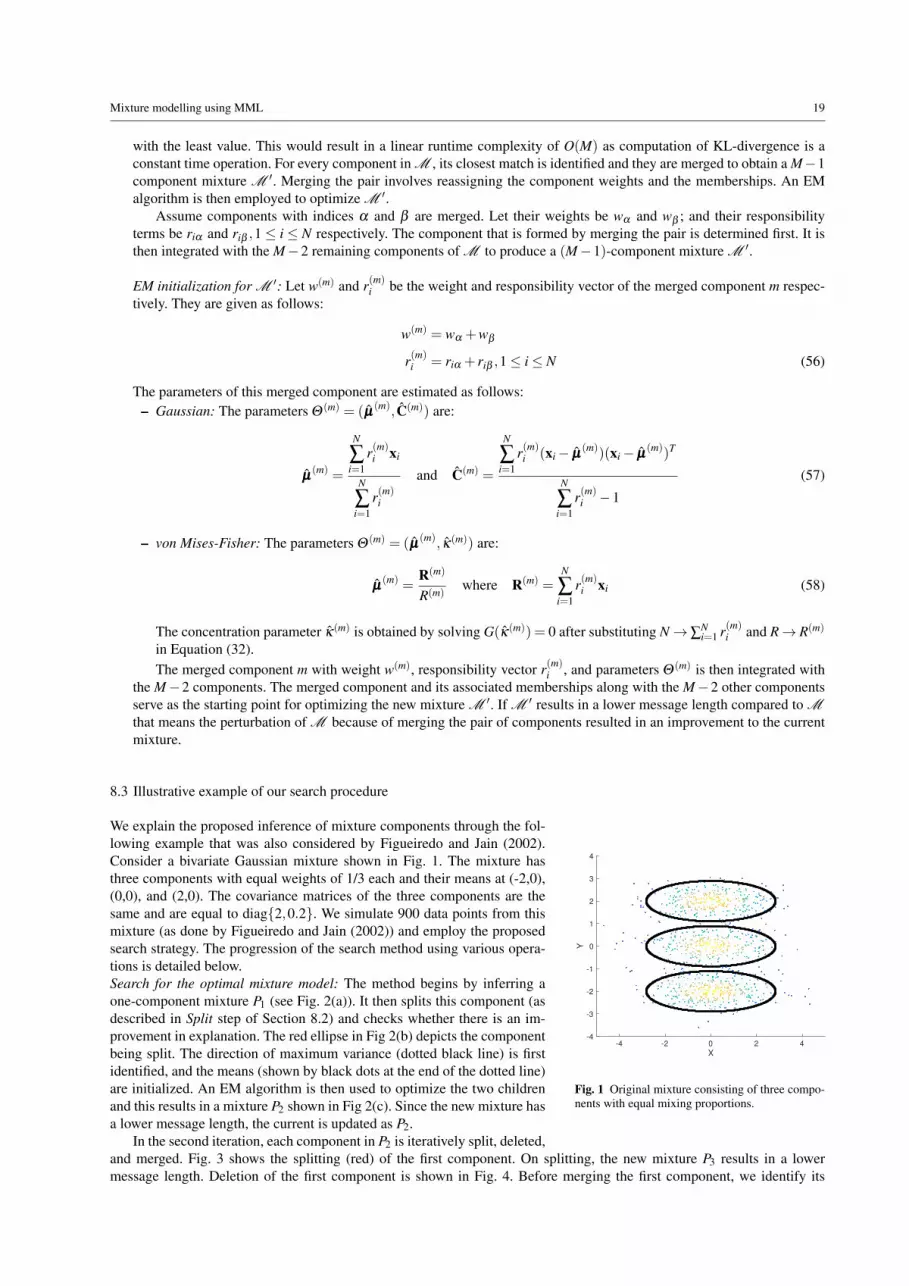
8.3 Illustrative example of our search procedure
X
-4 -2 0 2 4
Y
-4
-3
-2
-1
0
1
2
3
4
Fig. 1 Original mixture consisting of three compo-nents with equal mixing proportions.
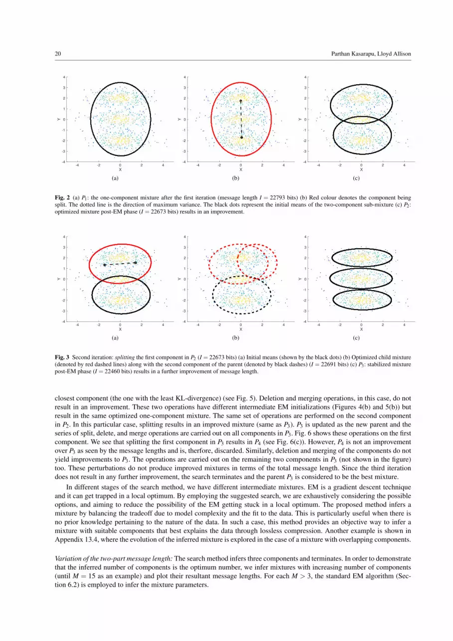
We explain the proposed inference of mixture components through the fol-lowing example that was also considered by Figueiredo and Jain (2002).Consider a bivariate Gaussian mixture shown in Fig. 1. The mixture hasthree components with equal weights of 1/3 each and their means at (-2,0),(0,0), and (2,0). The covariance matrices of the three components are thesame and are equal to diag{2,0.2}. We simulate 900 data points from thismixture (as done by Figueiredo and Jain (2002)) and employ the proposedsearch strategy. The progression of the search method using various opera-tions is detailed below.Search for the optimal mixture model: The method begins by inferring aone-component mixture P1 (see Fig. 2(a)). It then splits this component (asdescribed in Split step of Section 8.2) and checks whether there is an im-provement in explanation. The red ellipse in Fig 2(b) depicts the componentbeing split. The direction of maximum variance (dotted black line) is firstidentified, and the means (shown by black dots at the end of the dotted line)are initialized. An EM algorithm is then used to optimize the two childrenand this results in a mixture P2 shown in Fig 2(c). Since the new mixture hasa lower message length, the current is updated as P2.
In the second iteration, each component in P2 is iteratively split, deleted,and merged. Fig. 3 shows the splitting (red) of the first component. On splitting, the new mixture P3 results in a lowermessage length. Deletion of the first component is shown in Fig. 4. Before merging the first component, we identify its
20 Parthan Kasarapu, Lloyd Allison
X
-4 -2 0 2 4
Y
-4
-3
-2
-1
0
1
2
3
4
(a)X
-4 -2 0 2 4
Y
-4
-3
-2
-1
0
1
2
3
4
(b)X
-4 -2 0 2 4
Y
-4
-3
-2
-1
0
1
2
3
4
(c)
Fig. 2 (a) P1: the one-component mixture after the first iteration (message length I = 22793 bits) (b) Red colour denotes the component beingsplit. The dotted line is the direction of maximum variance. The black dots represent the initial means of the two-component sub-mixture (c) P2:optimized mixture post-EM phase (I = 22673 bits) results in an improvement.
X
-4 -2 0 2 4
Y
-4
-3
-2
-1
0
1
2
3
4
(a)X
-4 -2 0 2 4
Y
-4
-3
-2
-1
0
1
2
3
4
(b)X
-4 -2 0 2 4
Y
-4
-3
-2
-1
0
1
2
3
4
(c)
Fig. 3 Second iteration: splitting the first component in P2 (I = 22673 bits) (a) Initial means (shown by the black dots) (b) Optimized child mixture(denoted by red dashed lines) along with the second component of the parent (denoted by black dashes) (I = 22691 bits) (c) P3: stabilized mixturepost-EM phase (I = 22460 bits) results in a further improvement of message length.
closest component (the one with the least KL-divergence) (see Fig. 5). Deletion and merging operations, in this case, do notresult in an improvement. These two operations have different intermediate EM initializations (Figures 4(b) and 5(b)) butresult in the same optimized one-component mixture. The same set of operations are performed on the second componentin P2. In this particular case, splitting results in an improved mixture (same as P3). P3 is updated as the new parent and theseries of split, delete, and merge operations are carried out on all components in P3. Fig. 6 shows these operations on the firstcomponent. We see that splitting the first component in P3 results in P4 (see Fig. 6(c)). However, P4 is not an improvementover P3 as seen by the message lengths and is, therfore, discarded. Similarly, deletion and merging of the components do notyield improvements to P3. The operations are carried out on the remaining two components in P3 (not shown in the figure)too. These perturbations do not produce improved mixtures in terms of the total message length. Since the third iterationdoes not result in any further improvement, the search terminates and the parent P3 is considered to be the best mixture.
In different stages of the search method, we have different intermediate mixtures. EM is a gradient descent techniqueand it can get trapped in a local optimum. By employing the suggested search, we are exhaustively considering the possibleoptions, and aiming to reduce the possibility of the EM getting stuck in a local optimum. The proposed method infers amixture by balancing the tradeoff due to model complexity and the fit to the data. This is particularly useful when there isno prior knowledge pertaining to the nature of the data. In such a case, this method provides an objective way to infer amixture with suitable components that best explains the data through lossless compression. Another example is shown inAppendix 13.4, where the evolution of the inferred mixture is explored in the case of a mixture with overlapping components.
Variation of the two-part message length: The search method infers three components and terminates. In order to demonstratethat the inferred number of components is the optimum number, we infer mixtures with increasing number of components(until M = 15 as an example) and plot their resultant message lengths. For each M > 3, the standard EM algorithm (Sec-tion 6.2) is employed to infer the mixture parameters.

Mixture modelling using MML 21
X
-4 -2 0 2 4
Y
-4
-3
-2
-1
0
1
2
3
4
(a)X
-4 -2 0 2 4
Y
-4
-3
-2
-1
0
1
2
3
4
(b)X
-4 -2 0 2 4
Y
-4
-3
-2
-1
0
1
2
3
4
(c)
Fig. 4 Second iteration: deleting the first component in P2 (a) Green ellipse denotes the component being deleted (b) EM initialization with theremaining component (I = 25599 bits) (c) Resultant mixture after deletion and post EM (I = 22793 bits) – no improvement.
X
-4 -2 0 2 4
Y
-4
-3
-2
-1
0
1
2
3
4
(a)X
-4 -2 0 2 4
Y
-4
-3
-2
-1
0
1
2
3
4
(b)X
-4 -2 0 2 4
Y
-4
-3
-2
-1
0
1
2
3
4
(c)
Fig. 5 Second iteration: merging the two components in P2 (a) Blue ellipses denote the components currently being merged (b) EM initializationwith one merged component along with its parameters (c) Optimized mixture after merging (I = 22793 bits) – no improvement
22.35
22.40
22.45
22.50
22.55
22.60
22.65
22.70
22.75
22.80
2 4 6 8 10 12 140.02
0.04
0.06
0.08
0.10
0.12
0.14
0.16
0.18
0.20
0.22
Mes
sage
length
(in
thousa
nds
of
bit
s)
Number of components
first partsecond part
total
Fig. 7 Variation of the individual parts of the total message length with in-creasing number of components (note the two Y-axes have different scales– the first part follows the right side Y-axis; the second part and total mes-sage lengths follow the left side Y-axis)
Fig. 7 shows the total message lengths to which theEM algorithm converges for varying number of compo-nents M. As expected, the total message length (greencurve) drastically decreases initially until M = 3 compo-nents are inferred. Starting from M = 4, the total mes-sage length gradually increases, clearly suggesting thatthe inferred models are over-fitting the data with increas-ing statement cost to encode the additional parametersof these (more complex) models. We further elaborateon the reason for the initial decrease and subsequent in-crease in the total message length. As per MML eval-uation criterion, the message length comprises of twoparts – statement cost for the parameters and the cost forstating the data using those parameters. The model com-plexity (which corresponds to the mixture parameters) in-creases with increasing M. Therefore, the first part of themessage to encode parameters increases with an increasein the number of parameters. This behaviour is illustratedby the red curve in Fig. 7. The first part message lengthsare shown in red on the right side Y-axis in the figure. Asthe mixture model becomes increasingly more complex,the error of fitting the data decreases. This corresponds to the second part of the message in the MML encoding framework.This behaviour is consistent with what is observed in Fig. 7 (blue curve). There is a sharp fall until M = 3; then onwardsincreasing the model complexity does not lower the error significantly. The error saturates and there is minimal gain with

22 Parthan Kasarapu, Lloyd Allison
X
-4 -2 0 2 4
Y
-4
-3
-2
-1
0
1
2
3
4
(a) P3: parent (I = 22460 bits)X
-4 -2 0 2 4
Y
-4
-3
-2
-1
0
1
2
3
4
(b) Optimized children (I = 22480 bits)X
-4 -2 0 2 4
Y
-4
-3
-2
-1
0
1
2
3
4
(c) P4: mixture post-EM (I = 22474 bits)
X
-4 -2 0 2 4
Y
-4
-3
-2
-1
0
1
2
3
4
(d)X
-4 -2 0 2 4
Y
-4
-3
-2
-1
0
1
2
3
4
(e) Before optimizing (I = 25767 bits)X
-4 -2 0 2 4
Y
-4
-3
-2
-1
0
1
2
3
4
(f) Post-EM (I = 22610 bits)
X
-4 -2 0 2 4
Y
-4
-3
-2
-1
0
1
2
3
4
(g)X
-4 -2 0 2 4
Y
-4
-3
-2
-1
0
1
2
3
4
(h) Before optimizing (I = 22617 bits)X
-4 -2 0 2 4
Y
-4
-3
-2
-1
0
1
2
3
4
(i) Post-EM (I = 22610 bits)
Fig. 6 Third iteration: Operations involving the first component (a)-(c) denote the splitting process, (d)-(f) denote the deletion process, and (g)-(i)shows the merging of the first component with its closest component.
regards to encoding the data (the case of overfitting). However, the model complexity dominates after M = 3. The optimalbalance is achieved when M = 3. In summary, the message length at M = 3 components was rightly observed to be theoptimum for this example. We note that for a fixed number of mixture components, the EM algorithm for the MML metric ismonotonically decreasing. However, while searching for the number of components, MML continues to decrease until someoptimum is found and then steadily increases as illustrated through this example.
9 Experiments with Gaussian mixtures
We compare our proposed inference methodology against the widely cited method of Figueiredo and Jain (2002). The per-formance of their method is compared against that of Bayesian Information Criterion (BIC), Integrated Complete Likelihood(ICL), and approximate Bayesian (LEC) methods (discussed in Section 7). It was shown that the method of Figueiredo andJain (2002) was far superior than BIC, ICL and LEC (using Gaussian mixtures). In the following sections, we demonstratethrough a series of experiments that our proposed approach to infer mixtures fares better when compared to that of Figueiredoand Jain (2002). The experimental setup is as follows: we use a Gaussian mixture M t (true distribution), generate a random
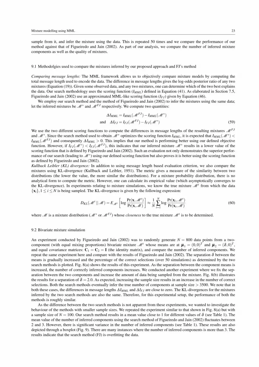
Mixture modelling using MML 23
sample from it, and infer the mixture using the data. This is repeated 50 times and we compare the performance of ourmethod against that of Figueiredo and Jain (2002). As part of our analysis, we compare the number of inferred mixturecomponents as well as the quality of mixtures.
9.1 Methodolgies used to compare the mixtures inferred by our proposed approach and FJ’s method
Comparing message lengths: The MML framework allows us to objectively compare mixture models by computing thetotal message length used to encode the data. The difference in message lengths gives the log-odds posterior ratio of any twomixtures (Equation (19)). Given some observed data, and any two mixtures, one can determine which of the two best explainsthe data. Our search methodology uses the scoring function (IMML) defined in Equation (41). As elaborated in Section 7.5,Figueiredo and Jain (2002) use an approximated MML-like scoring function (IFJ) given by Equation (46).
We employ our search method and the method of Figueiredo and Jain (2002) to infer the mixtures using the same data;let the inferred mixtures be M ∗ and M FJ respectively. We compute two quantities:
∆ IMML = IMML(MFJ)− IMML(M
∗)
and ∆ IFJ = IFJ(MFJ)− IFJ(M
∗) (59)
We use the two different scoring functions to compute the differences in message lengths of the resulting mixtures M FJ
and M ∗. Since the search method used to obtain M ∗ optimizes the scoring function IMML, it is expected that IMML(M ∗)<IMML(M FJ) and consequently ∆ IMML > 0. This implies that our method is performing better using our defined objectivefunction. However, if IFJ(M ∗) < IFJ(M FJ), this indicates that our inferred mixture M ∗ results in a lower value of thescoring function that is defined by Figueiredo and Jain (2002). Such an evaluation not only demonstrates the superior perfor-mance of our search (leading to M ∗) using our defined scoring function but also proves it is better using the scoring functionas defined by Figueiredo and Jain (2002).Kullback Leibler (KL) divergence: In addition to using message length based evaluation criterion, we also compare themixtures using KL-divergence (Kullback and Leibler, 1951). The metric gives a measure of the similarity between twodistributions (the lower the value, the more similar the distributions). For a mixture probability distribution, there is noanalytical form to compute the metric. However, one can calculate its empirical value (which asymptotically converges tothe KL-divergence). In experiments relating to mixture simulations, we know the true mixture M t from which the data{xi},1≤ i≤ N is being sampled. The KL-divergence is given by the following expression:
DKL(Mt ||M ) = EM t
[log
Pr(x,M t)
Pr(x,M )
]≈ 1
N
N
∑i=1
logPr(xi,M t)
Pr(xi,M )(60)
where M is a mixture distribution (M ∗ or M FJ) whose closeness to the true mixture M t is to be determined.
9.2 Bivariate mixture simulation
An experiment conducted by Figueiredo and Jain (2002) was to randomly generate N = 800 data points from a two-component (with equal mixing proportions) bivariate mixture M t whose means are at µµµ1 = (0,0)T and µµµ2 = (δ ,0)T ,and equal covariance matrices: C1 = C2 = I (the identity matrix), and compare the number of inferred components. Werepeat the same experiment here and compare with the results of Figueiredo and Jain (2002). The separation δ between themeans is gradually increased and the percentage of the correct selections (over 50 simulations) as determined by the twosearch methods is plotted. Fig. 8(a) shows the results of this experiment. As the separation between the component means isincreased, the number of correctly inferred components increases. We conducted another experiment where we fix the sep-aration between the two components and increase the amount of data being sampled from the mixture. Fig. 8(b) illustratesthe results for a separation of δ = 2.0. As expected, increasing the sample size results in an increase in the number of correctselections. Both the search methods eventually infer the true number of components at sample size > 3500. We note that inboth these cases, the differences in message lengths ∆ IMML and ∆ IFJ are close to zero. The KL-divergences for the mixturesinferred by the two search methods are also the same. Therefore, for this experimental setup, the performance of both themethods is roughly similar.
As the difference between the two search methods is not apparent from these experiments, we wanted to investigate thebehaviour of the methods with smaller sample sizes. We repeated the experiment similar to that shown in Fig. 8(a) but witha sample size of N = 100. Our search method results in a mean value close to 1 for different values of δ (see Table 1). Themean value of the number of inferred components using the search method of Figueiredo and Jain (2002) fluctuates between2 and 3. However, there is significant variance in the number of inferred components (see Table 1). These results are alsodepicted through a boxplot (Fig. 9). There are many instances where the number of inferred components is more than 3. Theresults indicate that the search method (FJ) is overfitting the data.

24 Parthan Kasarapu, Lloyd Allison
0
10
20
30
40
50
60
70
80
90
100
1.8 1.9 2 2.1 2.2 2.3 2.4 2.5 2.6
Corr
ect
sele
ctio
ns
(%)
Separation δ
ProposedFJ
(a)
1
1.2
1.4
1.6
1.8
2
2.2
500 1000 1500 2000 2500 3000 3500 4000
Aver
age
num
ber
of
infe
rred
com
ponen
ts
Number of data points
ProposedFJ
(b)
Fig. 8 2-dimensional mixture (a) Percentage of correct selections with varying separation for a fixed sample size of N = 800 (b) Average numberof inferred mixture components with different sample sizes and a fixed separation of δ = 2.0 between component means.
1
2
3
4
5
6
7
8
9
10
1.8 1.9 2.0 2.1 2.2 2.3 2.4 2.5 2.6
Nu
mb
er o
f in
ferr
ed c
om
po
nen
ts
Separation δ
ProposedFJ
Fig. 9 Box-whisker plot showing the variability in the number of in-ferred components (N = 100 and over 50 simulations).
Table 1 The mean and variance of the number of inferredcomponents for each δ value (N = 100 and over 50 simula-tions).
Separation Proposed FJδ Mean Variance Mean Variance
1.8 1.02 0.020 1.98 2.6731.9 1.00 0.000 2.26 2.4822.0 1.00 0.000 2.04 2.3252.1 1.02 0.020 2.20 3.5102.2 1.04 0.039 2.20 2.2852.3 1.06 0.057 2.44 3.6392.4 1.06 0.098 2.54 3.9672.5 1.04 0.039 2.98 3.2032.6 1.10 0.092 2.42 2.942
-60
-40
-20
0
20
40
1.8 1.9 2.0 2.1 2.2 2.3 2.4 2.5 2.6
Dif
fere
nce
in m
essa
ge
length
s
Separation δ
Proposed (∆IMML)
MML-like (∆IFJ)
Fig. 10 Bivariate mixture (N = 100): difference in message lengths com-puted using the two different scoring functions (see Equation (59)).
Further, we evaluate the correctness of the mix-tures inferred by the two search methods by compar-isons using the message length formulations and KL-divergence.Fig. 10 shows the boxplot of the difference inmessage lengths of the mixtures M ∗ inferred using ourproposed search method and the mixtures M FJ inferredusing that of Figueiredo and Jain (2002). ∆ IMML > 0across all values of δ for the 50 simulations. As per Equa-tion (59), we have IMML(M ∗) < IMML(M FJ). This im-plies that M ∗ has a lower message length compared toM FJ when evaluated using our scoring function. Simi-larly, we have ∆ IFJ < 0, i.e., IFJ(M ∗)> IFJ(M FJ). Thisimplies that M FJ has a lower message length comparedto M ∗ when evaluated using FJ’s scoring function. Theseresults are not surprising as M ∗ and M FJ are obtainedusing the search methods which optimize the respectiveMML and MML-like scoring functions.
We then analyzed the KL-divergence of M ∗ andM FJ with respect to the true bivariate mixture M t overall 50 simulations and across all values of δ . Ideally, theKL-divergence should be close to zero. Fig. 11(a) shows the KL-divergence of the mixtures inferred using the two search

Mixture modelling using MML 25
methods with respect to M t when the separation is δ = 2.0. The proposed search method infers mixtures whose KL-divergence (denoted by red lines) is close to zero, and more importantly less than the KL-divergence of mixtures inferred bythe search method of Figueiredo and Jain (2002) (denoted by blue lines). The same type of behaviour is noticed with othervalues of δ . Fig. 11(b) compares the KL-divergence for varying values of δ . The median value of the KL-divergence dueto the proposed search method is close to zero with not much variation. The search method of Figueiredo and Jain (2002)always result in KL-divergence higher than that of ours. The results suggest that, in this case, mixtures M FJ inferred byemploying the search method of Figueiredo and Jain (2002) deviate significantly from the true mixture distribution M t . Thiscan also be explained by the fact that there is a wide spectrum of the number of inferred components (Fig. 9). This suggeststhat the MML-like scoring function is failing to control the tradeoff between complexity and quality of fit, and hence, isselecting overly complex mixture models.
0
0.05
0.1
0.15
0.2
0.25
0.3
0.35
0.4
5 10 15 20 25 30 35 40 45 50
Em
pir
ical
KL
-div
ergen
ce
Iterations
ProposedFJ
(a)
0
0.1
0.2
0.3
0.4
0.5
0.6
1.8 1.9 2.0 2.1 2.2 2.3 2.4 2.5 2.6
Em
pir
ical
KL
-div
ergen
ce
Separation δ
Proposed
FJ
(b)
Fig. 11 Comparison of inferred mixtures using KL-divergence (bivariate example with N = 100 and 50 simulations) (a) Particular case of δ = 2.0(b) For all values of δ ∈ {1.8, . . . ,2.6}.
9.3 Simulation of 10-dimensional mixtures
Along the lines of the previous experiment, Figueiredo and Jain (2002) conducted another experiment for a 10-variate two-component mixture M t with equal mixing proportions. The means are at µµµ1 = (0, . . . ,0)T and µµµ2 = (δ , . . . ,δ )T , so that theEuclidean distance between them is δ
√10. The covariances of the two components are C1 = C2 = I (the identity matrix).
Random samples of size N = 800 were generated from the mixture and the number of inferred components are plotted. Theexperiment is repeated for different values of δ and over 50 simulations. Fig. 12(a) shows the number of inferred componentsusing the two search methods. At lower values of δ , the components are close to each other, and hence, it is relatively moredifficult to correctly infer the true number of components. We observe that our proposed method performs clearly betterthan that of Figueiredo and Jain (2002) across all values of δ . We also compared the quality of these inferred mixtures bycalculating the difference in message lengths using the two scoring functions and the KL-divergence with respect to M t
. For all values of δ , ∆ IMML > 0, i.e., our inferred mixtures M ∗ have a lower message length compared to M FJ whenevaluated using our scoring function. More interestingly, we also note that ∆ IFJ > 0 (see Fig. 13(a)). This reflects that M ∗
have a lower message length compared to M FJ when evaluated using the scoring function of Figueiredo and Jain (2002).This suggests that their search method results in a sub-optimal mixture M FJ and fails to infer the better M ∗.
In addition to the message lengths, we analyze the mixtures using KL-divergence. Similar to the bivariate example inFig. 11(a), the KL-divergence of our inferred mixtures M ∗ is lower than M FJ , the mixtures inferred by Figueiredo andJain (2002). Fig. 13(b) shows the boxplot of KL-divergence of the inferred mixtures M ∗ and M FJ . At higher values ofδ >= 1.45, the median value of KL-divergence is close to zero, as the number of correctly inferred components (Fig. 12(a))is more than 90%. However, our method always infers mixtures M ∗ with lower KL-divergence compared to M FJ . Theseexperimental results demonstrate the superior performance of our proposed search method.
Another experiment was carried out where the δ = 1.20 was held constant (extremely close components), graduallyincreased the sample size N, and plotted the average number of inferred components by running 50 simulations for eachN. Fig. 12(b) shows the results for the average number of inferred components as the amount of data increases. Our searchmethod, on average, infers the true mixture when the sample size is ∼ 1000. However, the search method of Figueiredo and
26 Parthan Kasarapu, Lloyd Allison
0
20
40
60
80
100
1.05 1.1 1.15 1.2 1.25 1.3 1.35 1.4 1.45 1.5 1.55 1.6
Corr
ect
sele
ctio
ns
(%)
Separation δ
ProposedFJ
(a)
1
1.2
1.4
1.6
1.8
2
2.2
600 800 1000 1200 1400 1600 1800 2000
Aver
age
num
ber
of
infe
rred
com
ponen
ts
Number of data points
ProposedFJ
(b)
Fig. 12 10-dimensional mixture: (a) Percentage of correct selections with varying δ for a fixed sample size of N = 800 (separation between themeans is δ
√10) (b) Average number of inferred mixture components with different sample sizes and δ = 1.20 between component means.
0
50
100
150
200
250
1.10 1.15 1.20 1.25 1.30 1.35 1.40 1.45 1.50 1.55 1.60
Dif
fere
nce
in m
essa
ge
length
s
Separation δ
Proposed (∆IMML)
MML-like (∆IFJ)
(a)
0.05
0.1
0.15
0.2
0.25
0.3
0.35
0.4
0.45
0.5
1.10 1.15 1.20 1.25 1.30 1.35 1.40 1.45 1.50 1.55 1.60
Em
pir
ical
KL
-div
ergen
ce
Separation δ
Proposed
FJ
(b)
Fig. 13 Comparison of mixtures with respect to the 10-variate true mixture and N = 800 (a) Difference in message lengths computed using the twoscoring functions (b) Box-whisker plot of KL-divergence
Jain (2002) requires larger amounts of data; even with a sample size of 2000, the average number of inferred components is∼ 1.9. In Fig. 12(b), the red curve reaches the true number of 2 and saturates more rapidly than the blue curve.
9.4 The impact of weight updates as formulated by Figueiredo and Jain (2002)
One of the drawbacks associated with the search method of Figueiredo and Jain (2002) is due to the form of the updatingexpression for the component weights (Equation (47)). As discussed in Section 7.5.2, a particular instance of wrong inferenceis bound to happen when the net membership of a (valid) component is less than Np/2, where Np is the number of freeparameters per component. In such a case, the component weight is updated as zero, and it is eliminated, effectively reducingthe mixture size by one.
We conducted the following experiment to demonstrate this behaviour: we considered the two-component 10-variatemixture M t as before and randomly generate samples of size 50 from the mixture. Since the constituent components ofM t have equal weights, on average, each component has a membership of 25. We used δ = {10,100,1000}, so that thetwo components are well apart from each other. For each δ , we run 50 simulations and analyze the number of inferredcomponents. As expected, the search method of Figueiredo and Jain (2002) always infer a mixture with one componentregardless of the separation δ . Our method always infers the correct number of components. In order to test the validity ofmixtures inferred by our proposed method, we analyze the resultant mixtures by comparing the message lengths as discussed

Mixture modelling using MML 27
in Section 9.1. Fig. 14(a) shows the difference in message lengths ∆ IMML given in Equation (59). We observe that ∆ IMML > 0
100
150
200
250
300
350
400
450
500
5 10 15 20 25 30 35 40 45 50
Dif
fere
nce
in
mes
sag
e le
ng
ths
Iterations
δ = 10δ = 100
δ = 1000
(a) ∆ IMML
100
150
200
250
300
350
400
450
500
550
5 10 15 20 25 30 35 40 45 50
Dif
fere
nce
in
mes
sag
e le
ng
ths
Iterations
δ = 10δ = 100
δ = 1000
(b) ∆ IFJ
Fig. 14 Evaluation of the quality of inferred mixtures by comparing the difference in message lengths as computed using the two scoring functions.Positive difference indicates that the mixtures inferred by our search method have lower message lengths (see Equation (59)).
for all δ . This demonstrates that our search based mixtures M ∗ have lower message lengths compared to mixtures M FJ
using our scoring function. The same phenomenon is observed when using the MML-like scoring function of Figueiredoand Jain (2002). In Fig. 14(b), we observe that ∆ IFJ > 0, which means our search based mixtures M ∗ have lower messagelengths compared to mixtures M FJ when evaluated using their scoring function.
2
4
6
8
10
12
10 100 1000
Em
pir
ical
KL
-div
erg
ence
Separation δ
Proposed
FJ
Fig. 15 Box-whisker plot of KL-divergence of mixtures inferredby the two search methods. A random sample of size N = 50 isgenerated for each δ and this is repeated 50 times.
This demonstrates that M ∗ is a better mixture as com-pared to M FJ and their search method is unable to infer it. Wealso note that the differences in message lengths increases withincreasing δ . This is because for the one-component inferredmixture M FJ , the second part of the message (Equation (46))which corresponds to the negative log-likelihood term increasesbecause of poorer fit to the data. The two modes in the data be-come increasingly pronounced as the separation between con-stituent components of the true mixture increases, and hence,modelling such a distribution using a one-component mixtureresults in a poorer fit. This is clearly an incorrect inference.
We further strengthen our case by comparing the KL-divergence of the inferred mixtures M ∗ and M FJ with re-spect to the true mixture. Fig. 15 illustrates the results. As δ in-creases, the blue coloured plots shift higher. These correspondto mixtures M FJ inferred by Figueiredo and Jain (2002). Oursearch method, however, infers mixtures M ∗ which have lowerKL-divergence. The figure indicates that the inferred mixturesM ∗ are more similar to the true distribution as compared tomixtures M FJ .
These experiments demonstrate the ability of our search method to perform better than the widely used method ofFigueiredo and Jain (2002). We compared the resulting mixtures using our proposed MML formulation and the MML-likeformulation of Figueiredo and Jain (2002), showing the advantages of the former over the latter. We also used a neutralmetric, KL-divergence, to establish the closeness of our inferred mixtures to the true distributions. We will now illustrate thebehaviour of our search method on two real world datasets.
9.5 Analysis of the computational cost
At any intermediate stage of the search procedure, a current mixture with M components requires M number of split, delete,and merge operations before it is updated. Each of the perturbations involve performing an EM to optimize the correspondingmixture parameters. To determine the convergence of EM, we used a threshold of 10−5 which was the same as used by
28 Parthan Kasarapu, Lloyd Allison
Figueiredo and Jain (2002). FJ’s method also requires to start from an initial large number of components. We used 25 asan initial number based on what was suggested in Figueiredo and Jain (2002). We investigate the number of times the EMroutine is called and compare it with that of Figueiredo and Jain (2002). We examine with respect to the simulations thatwere carried out previously. For the bivariate mixture discussed in Section 9.2, the number of resulting EM iterations whenthe sample sizes are N = 800 and N = 100 are compared in Fig. 16(a), (b) respectively.
0
50
100
150
200
250
1.8 1.9 2 2.1 2.2 2.3 2.4 2.5 2.6
EM
ite
rati
on
s
Separation δ
ProposedFJ
(a) Bivariate mixture (N = 800)
0
20
40
60
80
100
120
140
1.8 1.9 2 2.1 2.2 2.3 2.4 2.5 2.6
EM
ite
rati
on
s
Separation δ
ProposedFJ
(b) Bivariate mixture (N = 100)
10
15
20
25
30
35
40
45
50
55
1.1 1.2 1.3 1.4 1.5 1.6
EM
ite
rati
on
s
Separation δ
ProposedFJ
(c) 10-variate mixture (N = 800)
Fig. 16 Number of EM iterations performed during the mixture simulations discussed in Sections 9.2 and 9.3.
As per the discussion in Section 9.2, at N = 800, the average number of components inferred by the two methods areabout the same (Fig. 8(a)). However, the number of EM iterations required by FJ’s method is greater than 200 across allvalues of δ (Fig. 16(a)). In contrast, the proposed method, on average, requires fewer than 50 iterations. In this case, bothmethods produce a similar result with FJ’s method requiring more number of EM iterations. When the bivariate mixturesimulation is carried out using N = 100, the number of EM iterations required by FJ’s method, on average, is greater than100, while the proposed method requires fewer than 40 iterations (Fig. 16(b)). In this case, the proposed method not onlyinfers better mixtures (as discussed in Section 9.2) but is also conservative with respect to computational cost.
For the simulation results corresponding to the 10-variate mixtures in Section 9.3, the proposed method requires close to50 iterations on average, while FJ’s method requires about 20 (Fig. 16(c)). However, the mixtures inferred by the proposedmethod fare better when compared to that of FJ (Figs. 12, 13). Furthermore, for the simulation results explained in Sec-tion 9.4, FJ’s method stops after 3 EM iterations. This is because their program does not accommodate components when thememberships are less than Np/2. The proposed method requires 18 EM iterations on average and infers the correct mixturecomponents. In these two cases, our method infers better quality mixtures, with no significant overhead with regard to thecomputational cost.
9.6 Acidity data set (Richardson and Green, 1997; McLachlan and Peel, 1997)
The first example is the univariate acidity data set which contains 155 points. Our proposed search method infers a mixtureM ∗ with 2 components whereas the search method of Figueiredo and Jain (2002) infers a mixture M FJ with 3 components.The inferred mixtures are shown in Fig. 17 and their corresponding parameter estimates are given in Table 2. In order tocompare the mixtures inferred by the two search methods, we compute the message lengths of the inferred mixtures usingour complete MML and the approximated MML-like scoring functions.
When evaluated using our MML scoring function, our inferred mixture results in a gain of ∼ 4 bits (see Table 3). Basedon the MML framework, our two-component mixture M ∗ is 24 times more likely than the three-component mixture M FJ
(as per Equation (19)). Furthermore, when the inferred mixtures are evaluated as per the MML-like scoring function, M ∗
is still considered better (∼ 298 bits) than M FJ (∼ 320 bits). Thus, using both forms of scoring function, M ∗ is the bettermixture model of this data set.

Mixture modelling using MML 29
0
0.5
1
1.5
2
2.5 3 3.5 4 4.5 5 5.5 6 6.5 7 7.5 8
mixturecomponents
(a) Mixture M ∗ inferred using our proposed search method.
0
0.5
1
1.5
2
2.5 3 3.5 4 4.5 5 5.5 6 6.5 7 7.5 8
mixturecomponents
(b) Mixture M FJ inferred using FJ’s search method.
Fig. 17 Mixtures inferred by the two search methods using the acidity data set. See Table 2 for the corresponding parameter estimates.
Component Weight Parametersindex (µ,σ2)
1 0.41 6.24, 0.282 0.59 4.33, 0.14
(a) Proposed
Component Weight Parametersindex (µ,σ2)
1 0.34 6.39, 0.172 0.35 4.21, 0.053 0.31 4.71, 0.36
(b) FJ
Table 2 The parameters of the inferred mixtures shown in Fig. 17
Inferred mixturesScoring Proposed FJ
functions (M ∗) (M FJ)MML 1837.61 1841.69
MML-like 298.68 320.02
Table 3 Message lengths (measured in bits) of themixtures (in Fig. 17) as evaluated using the MML andMML-like scoring functions.
9.7 Iris data set (Anderson, 1935; Fisher, 1936)
The second example is the popular Iris data set. The data is 4-dimensional and comes from three Iris species namely, Iris-setosa, Iris-versicolor, and Iris-virginica. The data size is 150 with each class (species) comprising of 50 representativeelements. Our search method infers a 4 component mixture M ∗ and the search method of Figueiredo and Jain (2002) infersa 3 component mixture M FJ (see Fig. 18). Table 4 shows the memberships of the 150 elements in each of the componentsin the inferred mixtures. We notice an additional component M4 in M ∗ which has a net membership of 9.51, that is ∼ 6%of the entire data set. It appears that the component M2 in M FJ (Table 4(b)) is split into two components M2 and M4 inM ∗ (Table 4(a)). The quality of the inferred mixtures is determined by comparing their message lengths using the MMLand MML-like scoring functions. Table 5 shows the values obtained using the two formulations. When evaluated using ourcomplete MML formulation, our inferred mixture M ∗ results in extra compression of∼ 1 bit, which makes it twice as likelyas M FJ – it is a closely competing model compared to ours. When evaluated using the MML-like scoring function, ourinferred mixture still has a lower message length compared to M FJ . In both the cases, the mixture M ∗ inferred by oursearch method is preferred.
Species M1 M2 M3 M4setosa 50 0 0 0
versicolor 0 5.64 44.36 0virginica 0 40.29 0.20 9.51
(a) Data distribution using 4 components
Species M1 M2 M3setosa 50 0 0
versicolor 0 5.55 44.45virginica 0 49.78 0.22
(b) Data distribution using 3 components
Table 4 Memberships of Iris data as using the inferred mixtures in Fig. 18 (a) Distribution ofdata using M ∗ (b) Distribution of data using M FJ
Inferred mixturesScoring Proposed FJ
functions (M ∗) (M FJ)MML 6373.01 6374.27
MML-like 323.31 342.57
Table 5 Message lengths (measured in bits)of the mixtures (in Fig. 18) as evaluated us-ing the MML and MML-like scoring func-tions.

30 Parthan Kasarapu, Lloyd Allison
Principal component 1-4 -3 -2 -1 0 1 2 3 4 5
Prin
cip
al co
mp
on
en
t 2
-2
-1.5
-1
-0.5
0
0.5
1
1.5
setosaversicolorvirginica
(a) Mixture M ∗ inferred using our proposed search method.
Principal component 1-4 -3 -2 -1 0 1 2 3 4 5
Prin
cip
al co
mp
on
en
t 2
-2
-1.5
-1
-0.5
0
0.5
1
1.5
setosaversicolorvirginica
(b) Mixture M FJ inferred using FJ’s search method.
Fig. 18 Mixtures inferred by the two search methods using the Iris data set. The data is projected onto the two principal components.
10 Experiments with von Mises-Fisher distributions
We compare our MML-based parameter inference with the current state of the art vMF estimators (discussed in Section 3).Tests include the analysis of the MML estimates of the concentration parameter: κMN is the approximation of MML estimateusing Newton’s method and κMH is the approximation using Halley’s method (see Equations (33) and (34)) against thetraditionally used approximations. Estimation of the vMF mean direction is the same across all these methods. Estimation ofκ , however, differs and hence, the corresponding results are presented. Through these experiments, we demonstrate that theMML estimates perform better than its competitors. These are followed by experiments demonstrating how these estimatesaid in the inference of vMF mixtures. These experiments illustrate the application of the proposed search method to infervMF mixtures using empirical studies and on real world datasets.
10.1 MML-based parameter estimation for a vMF distribution
For different values of dimensionality d and concentration parameter κ , data of sample size N are randomly generated froma vMF distribution using the algorithm proposed by Wood (1994). The parameters of a vMF distribution are estimated usingthe previously mentioned approximations. Let κ = {κT ,κN ,κH ,κMN ,κMH} denote the estimate of κ due to the respectivemethods.
Errors in κ estimation: We first report the errors in κ estimation by calculating the absolute error |κ −κ| and the squarederror (κ −κ)2 averaged over 1000 simulations. The relative error |κ−κ|
κcan be used to measure the percentage error in κ
estimation. The following observations are made based on the results shown in Table 6.
– For N = 10,d = 10,κ = 10, the average relative error of κT ,κN ,κH is ∼ 25%; for κMN ,κMH , it is ∼ 20%. When Nis increased to 100, the average relative error of κT is 5.09%, κN ,κH is 5.05%, and κMN ,κMH is 4.9%. We note thatincreasing N while holding d and κ reduces the error rate across all estimation methods and for all tested combinationsof d,κ . This is expected because as more data becomes available, the inference becomes more accurate. The plots shownin Figure 19 reflect this behaviour. The mean error at lower values of N = 5,10,20,30 is noticeable. However, as N isincreased to 1000, there is a drastic drop in the error. We note that this behaviour is consistent across all the differentestimation methods.
– For fixed N and d, increasing κ increases the mean absolute error. However, the average relative error decreases. As anexample, for N = 100,d = 100,κ = 10, the average relative error of κT ,κN ,κH is ∼ 42%; for κMN ,κMH , it is 36.7% and34% respectively. When κ is increased to 100, the error rate for κT ,κN ,κH drops to 2.18% and for κMN ,κMH , it drops to1.68%. Further increasing κ by an order of magnitude to 1000 results in average relative errors of 1.4% for κT ,κN ,κHand 1.1% for κMN ,κMH . This indicates that as the data becomes more concentrated, the errors in parameter estimationdecrease.
– There does not appear to be a clear pattern of the variation in error rates when d is changed keeping N and κ fixed.However, in any case, MML-based approximations have the least mean absolute and mean squared error.
KL-divergence and message lengths of the estimates: The quality of parameter inference is further determined by computingthe KL-divergence and the message lengths associated with the parameter estimates. The analytical expression to calculate
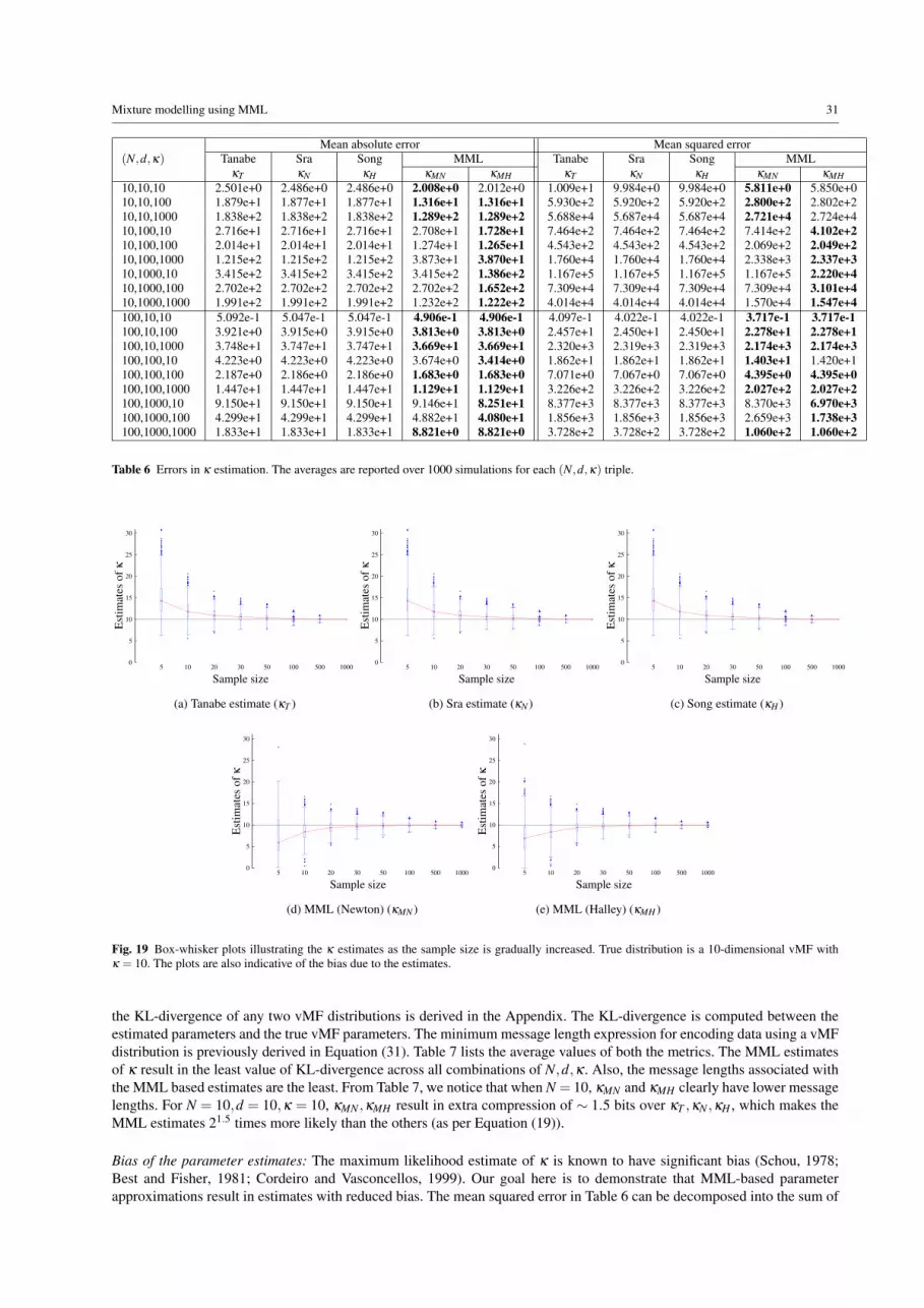
Mixture modelling using MML 31
(N,d,κ)Mean absolute error Mean squared error
Tanabe Sra Song MML Tanabe Sra Song MMLκT κN κH κMN κMH κT κN κH κMN κMH
10,10,10 2.501e+0 2.486e+0 2.486e+0 2.008e+0 2.012e+0 1.009e+1 9.984e+0 9.984e+0 5.811e+0 5.850e+010,10,100 1.879e+1 1.877e+1 1.877e+1 1.316e+1 1.316e+1 5.930e+2 5.920e+2 5.920e+2 2.800e+2 2.802e+210,10,1000 1.838e+2 1.838e+2 1.838e+2 1.289e+2 1.289e+2 5.688e+4 5.687e+4 5.687e+4 2.721e+4 2.724e+410,100,10 2.716e+1 2.716e+1 2.716e+1 2.708e+1 1.728e+1 7.464e+2 7.464e+2 7.464e+2 7.414e+2 4.102e+210,100,100 2.014e+1 2.014e+1 2.014e+1 1.274e+1 1.265e+1 4.543e+2 4.543e+2 4.543e+2 2.069e+2 2.049e+210,100,1000 1.215e+2 1.215e+2 1.215e+2 3.873e+1 3.870e+1 1.760e+4 1.760e+4 1.760e+4 2.338e+3 2.337e+310,1000,10 3.415e+2 3.415e+2 3.415e+2 3.415e+2 1.386e+2 1.167e+5 1.167e+5 1.167e+5 1.167e+5 2.220e+410,1000,100 2.702e+2 2.702e+2 2.702e+2 2.702e+2 1.652e+2 7.309e+4 7.309e+4 7.309e+4 7.309e+4 3.101e+410,1000,1000 1.991e+2 1.991e+2 1.991e+2 1.232e+2 1.222e+2 4.014e+4 4.014e+4 4.014e+4 1.570e+4 1.547e+4100,10,10 5.092e-1 5.047e-1 5.047e-1 4.906e-1 4.906e-1 4.097e-1 4.022e-1 4.022e-1 3.717e-1 3.717e-1100,10,100 3.921e+0 3.915e+0 3.915e+0 3.813e+0 3.813e+0 2.457e+1 2.450e+1 2.450e+1 2.278e+1 2.278e+1100,10,1000 3.748e+1 3.747e+1 3.747e+1 3.669e+1 3.669e+1 2.320e+3 2.319e+3 2.319e+3 2.174e+3 2.174e+3100,100,10 4.223e+0 4.223e+0 4.223e+0 3.674e+0 3.414e+0 1.862e+1 1.862e+1 1.862e+1 1.403e+1 1.420e+1100,100,100 2.187e+0 2.186e+0 2.186e+0 1.683e+0 1.683e+0 7.071e+0 7.067e+0 7.067e+0 4.395e+0 4.395e+0100,100,1000 1.447e+1 1.447e+1 1.447e+1 1.129e+1 1.129e+1 3.226e+2 3.226e+2 3.226e+2 2.027e+2 2.027e+2100,1000,10 9.150e+1 9.150e+1 9.150e+1 9.146e+1 8.251e+1 8.377e+3 8.377e+3 8.377e+3 8.370e+3 6.970e+3100,1000,100 4.299e+1 4.299e+1 4.299e+1 4.882e+1 4.080e+1 1.856e+3 1.856e+3 1.856e+3 2.659e+3 1.738e+3100,1000,1000 1.833e+1 1.833e+1 1.833e+1 8.821e+0 8.821e+0 3.728e+2 3.728e+2 3.728e+2 1.060e+2 1.060e+2
Table 6 Errors in κ estimation. The averages are reported over 1000 simulations for each (N,d,κ) triple.
0
5
10
15
20
25
30
5 10 20 30 50 100 500 1000
Est
imat
es o
f κ
Sample size
(a) Tanabe estimate (κT )
0
5
10
15
20
25
30
5 10 20 30 50 100 500 1000
Est
imat
es o
f κ
Sample size
(b) Sra estimate (κN )
0
5
10
15
20
25
30
5 10 20 30 50 100 500 1000
Est
imat
es o
f κ
Sample size
(c) Song estimate (κH )
0
5
10
15
20
25
30
5 10 20 30 50 100 500 1000
Est
imat
es o
f κ
Sample size
(d) MML (Newton) (κMN )
0
5
10
15
20
25
30
5 10 20 30 50 100 500 1000
Est
imat
es o
f κ
Sample size
(e) MML (Halley) (κMH )
Fig. 19 Box-whisker plots illustrating the κ estimates as the sample size is gradually increased. True distribution is a 10-dimensional vMF withκ = 10. The plots are also indicative of the bias due to the estimates.
the KL-divergence of any two vMF distributions is derived in the Appendix. The KL-divergence is computed between theestimated parameters and the true vMF parameters. The minimum message length expression for encoding data using a vMFdistribution is previously derived in Equation (31). Table 7 lists the average values of both the metrics. The MML estimatesof κ result in the least value of KL-divergence across all combinations of N,d,κ . Also, the message lengths associated withthe MML based estimates are the least. From Table 7, we notice that when N = 10, κMN and κMH clearly have lower messagelengths. For N = 10,d = 10,κ = 10, κMN ,κMH result in extra compression of ∼ 1.5 bits over κT ,κN ,κH , which makes theMML estimates 21.5 times more likely than the others (as per Equation (19)).
Bias of the parameter estimates: The maximum likelihood estimate of κ is known to have significant bias (Schou, 1978;Best and Fisher, 1981; Cordeiro and Vasconcellos, 1999). Our goal here is to demonstrate that MML-based parameterapproximations result in estimates with reduced bias. The mean squared error in Table 6 can be decomposed into the sum of

32 Parthan Kasarapu, Lloyd Allison
(N,d,κ)Average KL-divergence Average message length
Tanabe Sra Song MML Tanabe Sra Song MMLκT κN κH κMN κMH κT κN κH κMN κMH
10,10,10 8.777e-1 8.750e-1 8.750e-1 6.428e-1 6.445e-1 9.285e+2 9.285e+2 9.285e+2 9.269e+2 9.269e+210,10,100 8.803e-1 8.798e-1 8.798e-1 7.196e-1 7.199e-1 8.214e+2 8.214e+2 8.214e+2 8.208e+2 8.208e+210,10,1000 9.006e-1 9.005e-1 9.005e-1 7.443e-1 7.446e-1 6.925e+2 6.925e+2 6.925e+2 6.919e+2 6.919e+210,100,10 8.517e+0 8.517e+0 8.517e+0 8.479e+0 5.321e+0 8.633e+3 8.633e+3 8.633e+3 8.633e+3 8.585e+310,100,100 8.444e+0 8.444e+0 8.444e+0 6.007e+0 6.009e+0 8.428e+3 8.428e+3 8.428e+3 8.414e+3 8.414e+310,100,1000 8.472e+0 8.472e+0 8.472e+0 7.118e+0 7.120e+0 7.274e+3 7.274e+3 7.274e+3 7.269e+3 7.269e+310,1000,10 8.433e+1 8.433e+1 8.433e+1 8.433e+1 1.777e+1 7.030e+4 7.030e+4 7.030e+4 7.030e+4 6.925e+410,1000,100 8.430e+1 8.430e+1 8.430e+1 8.430e+1 4.697e+1 7.030e+4 7.030e+4 7.030e+4 7.030e+4 6.989e+410,1000,1000 8.451e+1 8.451e+1 8.451e+1 5.976e+1 5.977e+1 6.825e+4 6.825e+4 6.825e+4 6.811e+4 6.811e+4100,10,10 7.409e-2 7.385e-2 7.385e-2 7.173e-2 7.173e-2 9.115e+3 9.115e+3 9.115e+3 9.115e+3 9.115e+3100,10,100 7.539e-2 7.535e-2 7.535e-2 7.411e-2 7.411e-2 7.858e+3 7.858e+3 7.858e+3 7.858e+3 7.858e+3100 10,1000 7.271e-2 7.271e-2 7.271e-2 7.161e-2 7.161e-2 6.403e+3 6.403e+3 6.403e+3 6.403e+3 6.403e+3100,100,10 7.270e-1 7.270e-1 7.270e-1 6.146e-1 6.208e-1 8.615e+4 8.615e+4 8.615e+4 8.614e+4 8.614e+4100,100,100 7.357e-1 7.357e-1 7.357e-1 7.117e-1 7.117e-1 8.299e+4 8.299e+4 8.299e+4 8.299e+4 8.299e+4100,100,1000 7.330e-1 7.330e-1 7.330e-1 7.210e-1 7.210e-1 6.976e+4 6.976e+4 6.976e+4 6.976e+4 6.976e+4100,1000,10 7.324e+0 7.324e+0 7.324e+0 7.318e+0 6.201e+0 7.024e+5 7.024e+5 7.024e+5 7.024e+5 7.023e+5100,1000,100 7.302e+0 7.302e+0 7.302e+0 7.045e+0 7.106e+0 7.022e+5 7.022e+5 7.022e+5 7.019e+5 7.022e+5100,1000,1000 7.340e+0 7.340e+0 7.340e+0 7.097e+0 7.097e+0 6.707e+5 6.707e+5 6.707e+5 6.707e+5 6.707e+5
Table 7 Comparison of the κ estimates using KL-divergence and message length formulation (both metrics are measured in bits).
bias and variance terms as shown below (Taboga, 2012).
mean squared error = E[(κ−κ)2] = (E[κ]−κ)2︸ ︷︷ ︸Bias2(κ)
+E[(κ−E[κ])2]︸ ︷︷ ︸Variance(κ)
where E[.] denotes the expectation of the related quantity. Table 8 shows the bias-variance of the estimated concentrationparameter κ in the above simulations. The bias of κMN and κMH is lower compared to the other estimates. The variance ofthe MML estimates, however, is not always the least, as observed in Table 8. The combination of bias and variance, which isthe mean squared error, is empirically demonstrated to be the least for the MML estimates.
(N,d,κ)Bias (squared) Variance
Tanabe Sra Song MML Tanabe Sra Song MMLκT κN κH κMN κMH κT κN κH κMN κMH
10,10,10 5.609e+0 5.520e+0 5.520e+0 1.299e+0 1.269e+0 4.476e+0 4.464e+0 4.464e+0 4.512e+0 4.581e+010,10,100 2.298e+2 2.288e+2 2.288e+2 4.986e-3 2.577e-4 3.632e+2 3.632e+2 3.632e+2 2.800e+2 2.802e+210,10,1000 2.157e+4 2.156e+4 2.156e+4 2.764e+1 3.193e+1 3.531e+4 3.531e+4 3.531e+4 2.718e+4 2.720e+410,100,10 7.378e+2 7.378e+2 7.378e+2 7.333e+2 2.875e+2 8.660e+0 8.660e+0 8.660e+0 8.066e+0 1.226e+210,100,100 4.054e+2 4.053e+2 4.053e+2 1.546e+2 1.522e+2 4.894e+1 4.894e+1 4.894e+1 5.231e+1 5.273e+110,100,1000 1.473e+4 1.473e+4 1.473e+4 2.207e+1 1.994e+1 2.870e+3 2.870e+3 2.870e+3 2.316e+3 2.317e+310,1000,10 1.166e+5 1.166e+5 1.166e+5 1.166e+5 1.921e+4 8.090e+1 8.090e+1 8.090e+1 8.090e+1 2.983e+310,1000,100 7.301e+4 7.301e+4 7.301e+4 7.300e+4 2.728e+4 8.685e+1 8.685e+1 8.685e+1 8.635e+1 3.735e+310,1000,1000 3.964e+4 3.964e+4 3.964e+4 1.517e+4 1.493e+4 4.969e+2 4.969e+2 4.969e+2 5.306e+2 5.342e+2100,10,10 4.129e-2 3.528e-2 3.528e-2 8.132e-3 8.129e-3 3.684e-1 3.669e-1 3.669e-1 3.636e-1 3.636e-1100,10,100 1.280e+0 1.206e+0 1.206e+0 5.505e-2 5.504e-2 2.329e+1 2.329e+1 2.329e+1 2.273e+1 2.273e+1100,10,1000 9.796e+1 9.728e+1 9.728e+1 6.620e+0 6.619e+0 2.222e+3 2.222e+3 2.222e+3 2.168e+3 2.168e+3100,100,10 1.783e+1 1.783e+1 1.783e+1 4.661e+0 6.202e+0 7.807e-1 7.807e-1 7.807e-1 9.369e+0 8.003e+0100,100,100 3.371e+0 3.367e+0 3.367e+0 7.147e-1 7.146e-1 3.700e+0 3.700e+0 3.700e+0 3.681e+0 3.681e+0100,100,1000 1.161e+2 1.161e+2 1.161e+2 3.504e-1 3.504e-1 2.065e+2 2.065e+2 2.065e+2 2.023e+2 2.023e+2100,1000,10 8.372e+3 8.372e+3 8.372e+3 8.364e+3 6.809e+3 5.385e+0 5.385e+0 5.385e+0 5.200e+0 1.614e+2100,1000,100 1.848e+3 1.848e+3 1.848e+3 5.143e+2 1.628e+3 7.656e+0 7.656e+0 7.656e+0 2.145e+3 1.099e+2100,1000,1000 3.359e+2 3.359e+2 3.359e+2 6.926e+1 6.925e+1 3.692e+1 3.692e+1 3.692e+1 3.674e+1 3.674e+1
Table 8 Bias-variance decomposition of the squared error (κ−κ)2.
Statistical hypothesis testing: There have been several goodness-of-fit methods proposed in the literature to test the nullhypothesis of a vMF distribution against some alternative hypothesis (Kent, 1982; Mardia et al., 1984; Mardia and Jupp,2000). Recently, Figueiredo (2012) suggested tests for the specific case of concentrated vMF distributions. Here, we examinethe behaviour of κ estimates for generic vMF distributions as proposed by Mardia et al. (1984). They derived a likelihoodratio test for the null hypothesis of a vMF distribution (H0) against the alternative of a Fisher-Bingham distribution (Ha). Theasymptotically equivalent Rao’s score statistic (Rao, 1973) was used to test the hypothesis.

Mixture modelling using MML 33
The score statistic W , in this case, is a function of the concentration parameter. It has an asymptotic χ2(p) distribution(with degrees of freedom p = 1
2 d(d + 1)− 1) under H0 as the sample size N → ∞. For d = {10,100,1000}, the criticalvalues at 5% significance level are given in Table 9. If the computed test statistic exceeds the critical value, then the nullhypothesis of a vMF distribution is rejected. We conduct a simulation study where we generate random samples of size N = 1million from a vMF distribution with known mean and κ = {10,100,1000}. For each inferred estimate κ , we compute the teststatistic and compare it with the corresponding critical value. The results are shown in Table 9. For d = 10, the approximationκT has a significant effect as its test statistic exceeds the critical value and consequently the p-value is close to zero. Thisimplies that the null hypothesis of a vMF distribution is rejected by using the estimate κT . However, this is incorrect as thedata was generated from a vMF distribution. The p-values due to the estimates κN ,κH ,κMN ,κMH are all greater than 0.05 (thesignificance level) which implies that the null hypothesis is accepted. For d = {100,1000}, the p-values corresponding to thedifferent estimates are greater than 0.05. In these cases, the use of all the estimates lead to the same conclusion of acceptingthe null hypothesis of a vMF distribution. As the amount of data increases, the error due to all the estimates decreases. Thisis further exemplified below.
(d,κ)Critical Test statistic p-value of the testvalue Tanabe Sra Song MML Tanabe Sra Song MMLχ2(p) κT κN κH κMN κMH κT κN κH κMN κMH
10,10 7.215e+1 1.850e+2 5.353e+1 5.353e+1 5.353e+1 5.353e+1 0.000e+0 5.258e-1 5.258e-1 5.260e-1 5.260e-110,100 7.215e+1 1.698e+3 4.949e+1 4.949e+1 4.945e+1 4.945e+1 0.000e+0 6.247e-1 6.247e-1 6.267e-1 6.267e-110,1000 7.215e+1 1.950e+3 4.811e+1 4.811e+1 5.060e+1 5.060e+1 0.000e+0 6.571e-1 6.571e-1 5.724e-1 5.724e-1100,10 5.215e+3 5.090e+3 5.090e+3 5.090e+3 5.090e+3 5.090e+3 3.739e-1 3.739e-1 3.739e-1 3.741e-1 3.741e-1100,100 5.215e+3 5.010e+3 5.010e+3 5.010e+3 5.010e+3 5.010e+3 6.103e-1 6.127e-1 6.127e-1 6.125e-1 6.125e-1100,1000 5.215e+3 5.025e+3 5.018e+3 5.018e+3 5.022e+3 5.022e+3 5.427e-1 5.597e-1 5.597e-1 5.517e-1 5.517e-11000,10 5.021e+5 5.006e+5 5.006e+5 5.006e+5 5.006e+5 5.006e+5 4.682e-1 4.682e-1 4.682e-1 4.687e-1 4.687e-11000,100 5.021e+5 5.005e+5 5.005e+5 5.005e+5 5.005e+5 5.005e+5 5.050e-1 5.050e-1 5.050e-1 5.057e-1 5.057e-11000,1000 5.021e+5 5.007e+5 5.007e+5 5.007e+5 5.007e+5 5.007e+5 4.283e-1 4.283e-1 4.283e-1 4.196e-1 4.196e-1
Table 9 Goodness-of-fit tests for the null hypothesis H0 : vMF distribution and the alternate hypothesis Ha : Fisher-Bingham distribution. Criticalvalues of the test statistic correspond to a significance of 5%.
Asymptotic behaviour of MML estimates: Based on the empirical tests, we have so far seen that MML estimates fare betterwhen compared to the other approximations. We now discuss the behaviour of the MML estimates in the limiting case. Forlarge sample sizes (N→ ∞), we plot the errors in κ estimation. Song et al. (2012) demonstrated that their approximation κHresults in the lowest error in the limiting case. We compute the variation in error in two scenarios with fixed d = 1000 and:
1. increasing κ: Fig. 20(a) illustrates the behaviour of the absolute error with increasing κ . The first observation is thatirrespective of the estimation procedure, the error continues to increase with increasing κ values (which corroborates ourobservations in the empirical tests) and then saturates. According to Song et al. (2012), their estimate κH produces thelowest error which we can see in the figure. Further, our MML Newton approximation κMN actually performs worse thanSong’s approximation κH . However, we note that the errors due to MML Halley’s approximation κMH are identical tothose produced by κH . This suggests that asymptotically, the approximations achieved by κH and κMH are more accurate(note that the errors in the limiting case are extremely low).
2. increasing R: The maximum likelihood estimate of κ aims to achieve F(κ) ≡ Ad(κ)− R = 0 (Equation 10). Hence,log |Ad(κ)− R| gives a measure of the error corresponding to an estimate of κ . Figure 20(b) depicts the variation of thiserror with increasing R . We observe that κH and κMH produce the least error. We also note that the error produced dueto κMN is greater than that produced by κMH . However, we highlight the fact that MML-based parameter inference aimsto achieve G(κ) ≡ 0 (Equation 32), a fundamentally different objective function compared to the maximum likelihoodbased one.
The asymptotic results are shown here by assuming a value of N = 10200 (note the corresponding extremely low errorrates). In the limiting case, the MML estimate κMH coincides with the ML estimate κH . However, κH ’s performance isbetter compared to the MML Newton’s approximation κMN . The same behaviour is observed for when κ is fixed and thedimensionality is increased. For enormous amount of data, the ML approximations converge to the MML ones.
10.2 MML-based inference of mixtures of vMF distributions
An empirical study is carried out where the proposed search method is employed to infer a mixture using data sampled from aknown mixture distribution. The amount of data is gradually increased; for each sample size N, the simulation is repeated 50times and the number of inferred components is plotted (we used MML Halley’s approximation in all the discussed results).The various case studies are discussed below.
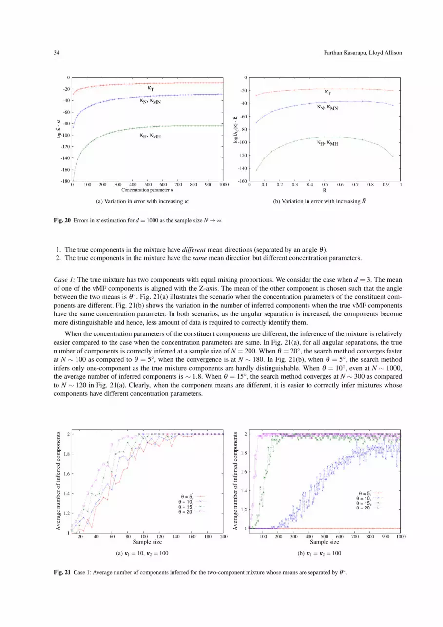
34 Parthan Kasarapu, Lloyd Allison
-180
-160
-140
-120
-100
-80
-60
-40
-20
0
0 100 200 300 400 500 600 700 800 900 1000
log
|κ -
κ|
Concentration parameter κ
κT
κN, κMN
κH, κMH
(a) Variation in error with increasing κ
-160
-140
-120
-100
-80
-60
-40
-20
0
0 0.1 0.2 0.3 0.4 0.5 0.6 0.7 0.8 0.9 1
log
|Ad(κ
) -
− R|
−R
κT
κN, κMN
κH, κMH
(b) Variation in error with increasing R
Fig. 20 Errors in κ estimation for d = 1000 as the sample size N→ ∞.
1. The true components in the mixture have different mean directions (separated by an angle θ ).2. The true components in the mixture have the same mean direction but different concentration parameters.
Case 1: The true mixture has two components with equal mixing proportions. We consider the case when d = 3. The meanof one of the vMF components is aligned with the Z-axis. The mean of the other component is chosen such that the anglebetween the two means is θ ◦. Fig. 21(a) illustrates the scenario when the concentration parameters of the constituent com-ponents are different. Fig. 21(b) shows the variation in the number of inferred components when the true vMF componentshave the same concentration parameter. In both scenarios, as the angular separation is increased, the components becomemore distinguishable and hence, less amount of data is required to correctly identify them.
When the concentration parameters of the constituent components are different, the inference of the mixture is relativelyeasier compared to the case when the concentration parameters are same. In Fig. 21(a), for all angular separations, the truenumber of components is correctly inferred at a sample size of N = 200. When θ = 20◦, the search method converges fasterat N ∼ 100 as compared to θ = 5◦, when the convergence is at N ∼ 180. In Fig. 21(b), when θ = 5◦, the search methodinfers only one-component as the true mixture components are hardly distinguishable. When θ = 10◦, even at N ∼ 1000,the average number of inferred components is ∼ 1.8. When θ = 15◦, the search method converges at N ∼ 300 as comparedto N ∼ 120 in Fig. 21(a). Clearly, when the component means are different, it is easier to correctly infer mixtures whosecomponents have different concentration parameters.
1
1.2
1.4
1.6
1.8
2
20 40 60 80 100 120 140 160 180 200
Aver
age
num
ber
of
infe
rred
com
ponen
ts
Sample size
θ = 5°
θ = 10°
θ = 15°
θ = 20°
(a) κ1 = 10, κ2 = 100
1
1.2
1.4
1.6
1.8
2
100 200 300 400 500 600 700 800 900 1000
Aver
age
num
ber
of
infe
rred
com
ponen
ts
Sample size
θ = 5°
θ = 10°
θ = 15°
θ = 20°
(b) κ1 = κ2 = 100
Fig. 21 Case 1: Average number of components inferred for the two-component mixture whose means are separated by θ ◦.

Mixture modelling using MML 35
Case 2: In this case, multivariate (d = {2,3,10}) vMF mixtures with equal mixing proportions and same component meansare considered. The simulation results of true mixtures with two and three components are presented here.
Fig. 22(a) shows the average number of components inferred for a two-component mixture whose concentration param-eters are κ1 = 10 and κ2 = 100. For each value of d, as the sample size increases, the average number of inferred componentsgradually increases until it saturates and reaches the true value (2 in this case). Increasing the sample size beyond this doesnot impact the number of inferred mixture components. The results for a 3-component mixture with identical means andconcentration parameters κ1 = 10,κ2 = 100, and κ3 = 1000 are shown in Fig. 22(b). As expected, the average number ofinferred components increases in light of greater evidence. However, we note that it requires greater amount of data to cor-rectly infer the three mixture components as compared to the two-component case. In the two-component case (Fig. 22(a)),at around N = 450, all the three curves converge to the right number of components. For the three-component mixture inFig. 22(b), up until N = 500, there is no convergence for d = 2,3. For d = 10, the average number of inferred componentsconverges quickly (at N ∼ 25) for the 2-component mixture when compared with N ∼ 100 for the 3-component mixture.This is expected as correctly distinguishing three components (with same means) requires far more data.
1
1.2
1.4
1.6
1.8
2
50 100 150 200 250 300 350 400 450 500
Aver
age
num
ber
of
infe
rred
com
ponen
ts
Sample size
d = 2
d = 3
d = 10
(a) 2-component mixture
1
1.5
2
2.5
3
50 100 150 200 250 300 350 400 450 500
Aver
age
num
ber
of
infe
rred
com
ponen
ts
Sample size
d = 2
d = 3
d = 10
(b) 3-component mixture
Fig. 22 Case 2: Average number of components inferred when the true mixture has components with the same mean directions but differentconcentration parameters. (a) 2-component mixture (κ1 = 10,κ2 = 100) (b) 3-component mixture (κ1 = 10,κ2 = 100,κ3 = 1000)
It is also interesting to note that for d = 2 in Fig. 22(b), the average number of inferred components saturates at 2, whilethe actual number of mixture components is 3. However, as the amount of available data increases, the (almost) horizontalline shows signs of gradual increase in its slope. Fig. 23 shows the increase in the average number for d = 2,3 as the data isincreased beyond N = 500. The blue curve representing d = 3 stabilizes at N ∼ 2500. However, the red curve (d = 2) slowlystarts to move up but the average is still well below the true number. This demonstrates the relative difficulty in estimatingthe true mixture when the means coincide especially at lower dimensions.
2
2.2
2.4
2.6
2.8
3
500 1000 1500 2000 2500
Av
erag
e n
um
ber
of
infe
rred
co
mp
on
ents
Sample size
d = 2
d = 3
Fig. 23 Gradual increase in the average inferred components forthe 3-component mixture in Fig. 22(b).
One can imagine that when the means coincide, it wouldrequire greater amount of data to accurately infer the true mix-ture components. However, the amount of data required alsodepends on the dimensionality in consideration. It appears thatas the dimensionality increases, we need smaller amounts ofdata (as can be seen for the d = 10 case). In d-dimensionalspace, each datum comprises of d real values with the con-straint that it should lie on the unit hypersphere. So the esti-mation of the mean direction requires the estimation of (d−1)values and one value for κ . When there is N data, we actu-ally have nd = N× (d− 1) values available for estimating thed free parameters. For instance, given a sample of size N, ford = 2,n2 = N and for d = 10,n10 = 9N. We conjecture that thiscould be a possible reason for faster convergence in high di-mensional space. Through these experiments, we have demon-strated the ability of our search method to infer appropriatemixtures in situations with varying difficulty levels.

36 Parthan Kasarapu, Lloyd Allison
11 Applications of vMF mixtures
11.1 Application to text clustering
The use of vMF mixtures in modelling high dimensional textdata has been investigated by Banerjee et al. (2005). To compute the similarity between text documents requires their rep-resentation in some vector form. The elements of the vectors are typically a function of the word and document frequenciesin a given collection. These vector representations are commonly used in clustering textual data with cosine based similaritymetrics being central to such analyses (Strehl et al., 2000). There is a strong argument for transforming the vectors intopoints on a unit hypersphere (Salton and McGill, 1986; Salton and Buckley, 1988). Such a normalized representation of textdata (which compensates for different document lengths) motivates their modelling using vMF mixture distributions.
Banerjee et al. (2005) used their proposed approximation (Equation (12)) to estimate the parameters of a mixture withknown number of components. They did not, however, propose a method to search for the optimal number of mixturecomponents. We not only derived MML estimates which fare better compared to the previous approximations but alsoapply them to devise a search method to infer the optimal mixtures. Ideally, the search is continued until there is no furtherimprovement in the message length (Algorithm 1). For practial purposes, the search is terminated when the improvement dueto the intermediate split, delete and merge operations during the search process is less than 0.01%. Our proposed method toinfer mixtures was employed on the datasets that were used in the analysis by Banerjee et al. (2005). The parameters of theintermediate mixtures are estimated using the MML Halley’s estimates (Equation (34)) for the component vMF distributions.Banerjee et al. (2005) use mutual information (MI) to assess the quality of clustering. For given cluster assignments X and
the (known) class labels Y , MI is defined as: E[
logPr(X ,Y )
Pr(X)Pr(Y )
]. Along with the message lengths, we use MI as one other
evaluation criterion in our analysis. We also compute the average F-measure when the number of clusters is same as thenumber of actual classes.
For each of the datasets, in the preprocessing step, we generate feature vectors using the most frequently occuring wordsand generating a TF-IDF score for each feature (word) based on Okapi BM25 score (Robertson and Zaragoza, 2009). Thesefeature vectors are then normalized to generate unit vectors in some d-dimensional space. Using this as directional data on ahypersphere, a suitable mixture model was inferred using the greedy search proposed in Section 8.
11.1.1 Classic3 dataset
The dataset2 contains documents from three distinct categories: 1398 Cranfield (aeronautical related), 1033 Medline (medicaljournals) and 1460 Cisi (information retrieval related) documents. The processed data has d = 4358 features.Optimal number of clusters: In this example, it is known that there are three distinct categories. However, this informationis not usually known in real world setting (and we do not know if they are from three vMF distributions). Assuming noknowledge of the nature of the data, the search method infers a mixture with 16 components. The corresponding assignmentsare shown in Table 10. A closer look at the generated assignments illustrate that each category of documents is represented bymore than one component. The three categories are split to possibly represent specialized sub-categories. The Cisi categoryis distributed among 6 main components (M4 – M9). The Cranfield documents are distributed among M6, M10 – M15components and the Medline category is split into M0 – M3, and M6 components. We observe that all but three componentsare non-overlapping; only M6 has representative documents from all three categories.
M0 M1 M2 M3 M4 M5 M6 M7 M8 M9 M10 M11 M12 M13 M14 M15cisi 0 0 4 0 288 133 28 555 197 255 0 0 0 0 0 0cran 0 0 0 0 2 0 362 1 0 0 58 144 135 175 223 298med 9 249 376 138 2 0 9 0 0 0 0 0 0 0 0 0
Table 10 Confusion matrix for 16-component assignment (MML Halley).
The 16-component mixture inferred by the search method is a finer segregation of the data when compared to modellingusing a 3-component mixture. The parameters of the 3-component mixture are estimated using an EM algorithm (Sec-tion 6.2). Table 11 shows the confusion matrices obtained for the cluster assignments using the various estimation methods.We see that all the estimates perform comparably with each other; there is not much difference in the assignments of data tothe individual mixture components.
The collection is comprised of documents that belong to dissimilar categories and hence, the clusters obtained are wideapart. This can be seen from the extremely high F-measure scores (Table 12). For the 3-component mixture, all the fivedifferent estimates result in high F-measure values with Song being the best with an average F-measure of 0.978 and a MI
2 http://www.dataminingresearch.com/index.php/2010/09/classic3-classic4-datasets/

Mixture modelling using MML 37
cisi cran medcisi 1441 0 19cran 22 1293 83med 8 0 1025
(a) Banerjee
cisi cran medcisi 1449 0 11cran 24 1331 43med 13 0 1020
(b) Tanabe
cisi cran medcisi 1450 0 10cran 24 1339 35med 14 0 1019
(c) Song
cisi cran medcisi 1450 0 10cran 24 1331 43med 13 0 1020
(d) MML (Halley)
Table 11 Confusion matrices for 3-cluster assignment. (Sra’s confusion matrix is omitted as it is same as that of Tanabe)
of 0.982. MML (Halley’s) estimate are close with an average F-measure of 0.976 and a MI of 0.976. However, based on themessage length criterion, the MML estimate results in the least message length (∼ 190 bits less than Song’s). The mutualinformation score using MML estimate is 1.04 (for 16 components) compared to 0.976 for 3 components. Also, the messagelength is lower for the 16 component case. However, Song’s estimator results in a MI score of 1.043, very close to the scoreof 1.040 obtained using MML estimates.
Number of clusters Evaluation metric Banerjee Tanabe Sra Song MML (Halley)
3Message length 100678069 100677085 100677087 100677080 100676891Avg. F-measure 0.9644 0.9758 0.9758 0.9780 0.9761
Mutual Information 0.944 0.975 0.975 0.982 0.976
16 Message length 100458153 100452893 100439983 100444649 100427178Mutual Information 1.029 1.036 0.978 1.043 1.040
Table 12 Clustering performance on Classic3 dataset.
For the Classic3 dataset, Banerjee et al. (2005) analyzed mixtures with greater numbers of components than the “natural”number of clusters. They report that a 3-component mixture is not necessarily a good model and more number of clustersmay be preferred for this example. As part of their observations, they suggest to “generate greater number of clusters andcombine them appropriately”. However, this is subjective and requires some background information about the likely numberof clusters. Our search method in conjunction with the inference framework is able to resolve this dilemma and determinethe optimal number of mixture components in a completely unsupervised setting.
11.1.2 CMU Newsgroup
The dataset3 contains documents from 20 different news categories each containing 1000 documents. Preprocessing ofthe data, as discussed above, resulted in feature vectors of dimensionality d = 6448. The data is first modelled using amixture containing 20 components. The evaluation metrics are shown in Table 13. The average F-measure is 0.509 for MML-based estimation, slightly better than Banerjee’s score of 0.502. The low F-measure values are indicative of the difficulty inaccurately distinguishing the news categories. The mutual information score for MML case is 1.379 which is lower than thatof Sra’s. However, the total message length is lower for MML mixture compared to that of others.
Number of clusters Evaluation metric Banerjee Tanabe Sra Song MML (Halley)
20Message length 728666702 728545471 728585441 728536451 728523254Avg. F-measure 0.502 0.470 0.487 0.435 0.509
Mutual Information 1.391 1.383 1.417 1.244 1.379
21 Message length 728497453 728498076 728432625 728374429 728273820Mutual Information 1.313 1.229 1.396 1.377 1.375
Table 13 Clustering performance on CMU Newsgroup dataset.
Optimal number of clusters: The proposed search method when applied to this dataset infers a mixture with 21 components.This is close to the “true” number of 20 (although there is no strong reason to believe that each category corresponds to avMF component). The mutual information for the 21-cluster assignment is highest for Sra’s mixture with a score of 1.396and for MML mixture, it is 1.375 (Table 13). However, the total message length is the least for the MML-based mixture.
The analysis of vMF mixtures by Banerjee et al. (2005) for both the datasets considered here shows a continued increasein the MI scores even beyond the true number of clusters. As such, using the MI evaluation metric for different number ofmixture components does not aid in the inference of an optimal mixture model. Our search method balances the tradeoff
3 http://archive.ics.uci.edu/ml/datasets/Twenty+Newsgroups

38 Parthan Kasarapu, Lloyd Allison
between using a certain mixture and its ability to explain the observed data, and thus, objectively aids in inferring mixturesto model the normalized vector representations of a given collection of text documents.
A mixture modelling problem of this kind where there is some information available regarding the nature of the data canbe studied by altering the proposed search method. We provide some alternate strategies where the mixture modelling canbe done in a semi-supervised setting.
– The priors on the number of components and their parameters can be modelled based on the background knowledge.– If the true number of clusters are known, only splits may be carried out until we near the true number (each split being
the best one given the current mixture). As the mixture size approaches the true number, all the three operations (split,delete, and merge) can be resumed until convergence. This increases the chance that the inferred mixture would haveabout the same number of components as the true model.
– Another variant could be to start from a number close to the true number and prefer delete/merge operations over thesplits. We cannot ignore splits completely because a component after splitting may be merged at a later iteration if therewould be an improvement to the message length.
– Another strategy could be to employ the EM algorithm and infer a mixture with the true number of components. Thismixture can then be perturbed using split, delete, and merge operations until convergence.
11.2 Mixture modelling of protein coordinate data
The following application concerns the vMF mixture modelling of directional data arising from the orientation of main chaincarbon atoms in protein structures. The structures that proteins adopt are largely dictated by the interactions between the con-stituent atoms. These chemical interactions impose constraints on the orientation of atoms with respect to one another. Thedirectional nature of the protein data and the (almost constant) bond length between the main chain carbon atoms motivatethe modelling using vMF mixtures. Further, structural modelling tasks such as generating random protein chain confor-mations, three-dimensional protein structure alignment, secondary structure assignment, and representing protein foldingpatterns using concise protein fragments require efficient encoding of protein data (Konagurthu et al., 2012, 2013; Collieret al., 2014). As part of our results, we demonstrate that vMF mixtures offer a better means of encoding and can potentiallyserve as strong candidate models to be used in such varied tasks.
The dataset considered here is a collection of 8453 non-redundant experimentally determined protein structures from thepublicly available ASTRAL SCOP-40 (version 1.75) database (Murzin et al., 1995). For each protein structure, the coordi-nates of the central carbon, Cα , of successive residues (amino acids) are considered. Protein coordinate data is transformedinto directional data and each direction vector is characterized by (θ ,φ) = (co-latitude, longitude), where θ ∈ [0,180◦] andφ ∈ [0,360◦]. Note that these (θ ,φ) values have to be measured in a consistent, canonical manner.
Fig. 24 Canonical orientation used to determine the directionaldata corresponding to protein coordinates.
To compute (θ ,φ) corresponding to the point Pi+1 associ-ated to residue i+ 1, we consider this point in the context of3 preceding points, forming a 4-mer comprising of the pointsPi−2,Pi−1,Pi, and Pi+1. This 4-mer is orthogonally transformedinto a canonical orientation (Fig. 24) in the following steps:
– translate the 4-mer such that Pi is at the origin.– rotate the resultant 4-mer so that Pi−1 lies on the negative
X-axis.– rotate further so that Pi−2 lies in the XY plane such that
the angle between the vector Pi−2−Pi−1 and the positiveY-axis is acute.
The transformation yields a canonical orientation for Pi+1 withrespect to its previous 3 coordinates. Using the transformed co-ordinates of Pi+1, the direction (θ ,φ) of Pi+1 is computed. Werepeat this transformation for every successive set of 4-mersin the protein chain, over all possible source structures in ourcollection. The data collected in this way resulted in a totalof ∼ 1.3 million (θ ,φ) pairs for all the 8453 structures in thedatabase.
Protein data is an example where the number of mixture components are not known a priori. Hence, we use the methodoutlined in Section 8 to infer suitable mixture models. The original dataset comprises of 7 different categories of proteins.The proposed search method using MML (Halley’s) estimates infers a mixture containing 13 vMF components. Further,each protein category can be individually modelled using a mixture. As an example, for the “β class” proteins which con-tains 1802 protein structures and 251,346 corresponding (θ ,φ) pairs, our search method terminates after inferring 11 vMFcomponents. We compare the MML-based mixtures with those inferred by the standalone EM algorithm (Section 6.2) using

Mixture modelling using MML 39
other estimates. These values are presented in Table 14. We observe that the mixtures inferred using the MML estimatesresult in a message length lower than that obtained using the other estimates.
Fig. 25(a) shows the empirical distribution of directional data of Cα coordinates belonging to β class. The (θ ,φ) valueswith their corresponding frequencies are plotted in Fig. 25(a). Fig. 25(b) is a plot illustrating the 11-component vMF mixturedensity as inferred for this class of proteins. Notice that the two major modes in the figure correspond to commonly observedlocal secondary structural bias of residues towards, helices and strands of sheet. Also notice the empty region in the middlewhich corresponds to physically unrealizable directions in the local chain, excluded in the observed samples due to sterichindrance of the atoms in proteins. If we were to model such data using truncated distributions, the regions of zero probabilitywill be modelled using an infinite code length. As an example, at (θ ,φ) = (100◦,200◦), the truncated distribution would havezero probability and consequently an infinite code length. However, when the same point is explained using the 11-componentmixture, it would have a probability of Pr = 3.36× 10⁻¹² and a corresponding code length of − log2 Pr = 38.11 bits. Forprotein data, it is possible to have such (rare exceptional) observations, due to reasons such as experimental error, noise, orthe conformation of the protein itself. Hence, although the empirical distribution has distinct modes, it is better off modelledas a vMF mixture distribution, rather than by truncated distributions.
(a) (b)
Fig. 25 Distribution of directional data of β class Cα atoms (a) Empirical distribution (b) Mixture density corresponding to the 11 inferred vMFcomponents
Compressibility of protein structures: The explanatory framework of MML allows for testing competing hypotheses. Re-cently, Konagurthu et al. (2012) developed a null model description of protein coordinate data as part of the statisticalinference of protein secondary structure. A null model gives a baseline for transmitting the raw coordinate data. Each Cα
atom is described using the distance and orientation with respect to the preceding Cα atoms. Because the distance betweensuccessive Cα atoms is highly constrained, compression can only be gained in describing the orientation of a Cα atom withrespect to its previous one.
Konagurthu et al. (2012) describe their null hypothesis by discretizing the surface of a 3D-sphere into chunks of equalareas (of ε2, where ε is the accuracy of measurement of coordinate data). This results in 4πr2/ε2 cells distributed uniformlyon the surface of the sphere of radius r (the distance between successive Cα coordinates). The cells are uniquely numbered.To encode Ci+1
α with respect to Ciα , the location of Ci+1
α on the surface is identified and the corresponding cell index isencoded. Using this description, the stated null model results in a message length expression Konagurthu et al. (2012) givenby
Uniform Null =− log2
(ε2
4πr2
)= log2(4π)−2log2
(ε
r
)bits. (61)
The null model of Konagurthu et al. (2012) assumes a uniform distribution of orientation angles on the surface of thesphere. However, this is a crude assumption and one can leverage the directional properties of protein coordinates to buildan efficient null model. To this effect, we explore the use of vMF mixtures as null model descriptors for protein structures.Using vMF mixtures, we encode the co-latitude (θ ) and longitude (φ ) angles (described in Section 11.2). The message lengthexpression to encode the orientation angles (using Equation 1) is then given by
vMF Null =− log2
(M
∑j=1
w j f j(x;Θ j)
)−2log2
(ε
r
)bits. (62)

40 Parthan Kasarapu, Lloyd Allison
where x corresponds to a unit vector described by (θ ,φ) on the surface of the sphere. Equations (61) and (62) are twocompeting null models. These are used to encode the directional data corresponding to the 8453 protein structures in theASTRAL SCOP-40 database. The results are shown in Table 15.
Category Tanabe Sra Song MML (Halley)β 5514800 5518679 5520073 5513507
All 27818524 27833704 27839802 27803427
Table 14 Message lengths (in bits) computed for the inferred protein mix-tures using various methods (‘All’ refers to all the 7 protein categories).
Null model Total message length (in bits) Bits per residueUniform 36119900 27.437
vMF 32869700 24.968
Table 15 Comparison of the uniform and vMF null model encod-ing schemes.
The per residue statistic is calculated by dividing the total message length by the sample size (the number of (θ ,φ) pairs).This statistic shows that close to 2.5 bits can be saved (on average) if the protein data is encoded using the vMF null model.The vMF null model thus supercedes the naive model of encoding. This can potentially improve the accuracy of statisticalinference that is central to the various protein modelling tasks briefly introduced above.
12 Conclusion
We presented a statistically robust approach for inferring mixtures of (i) multivariate Gaussian distributions, and (ii) vonMises-Fisher distributions for d-dimensional directional data. It is based on the general information-theoretic frameworkof minimum message length inference. This provides an objective tradeoff between the hypothesis complexity and thequality of fit to the data. An associated search procedure for an optimal mixture model of given data chooses the number ofcomponent distributions, M, by minimizing the total message length. We established the better performance of the proposedsearch algorithm by comparing with a popularly used search method (Figueiredo and Jain, 2002). We demonstrated theeffectiveness of our approach through extensive experimentation and validation of our results. We also applied our methodto real-world high dimensonal text data and to directional data that arises from protein chain conformations. The experimentalresults demonstrate that our proposed method fares better when compared with the current state of the art techniques.
Acknowledgements The authors would like to thank Arun Konagurthu for discussions pertaining to protein data clustering, and Maria Garcia dela Banda for stimulating discussions and providing interesting insights. The authors would also like to acknowledge Wray Buntine’s inputs withregard to text clustering.
Bibliography
Agusta Y, Dowe DL (2003) Unsupervised learning of correlated multivariate Gaussian mixture models using MML. In: AI2003: Advances in Artificial Intelligence, Springer, Berlin, Heidelberg, pp 477–489
Akaike H (1974) A new look at the statistical model identification. IEEE Transactions on Automatic Control, 19(6):716–723Anderson E (1935) The Irises of the Gaspe Peninsula. Bulletin of the American Iris Society 59:2–5Banerjee A, Dhillon I, Ghosh J, Sra S (2003) Generative model-based clustering of directional data. In: Proceedings of the
9th International Conference on Knowledge Discovery and Data Mining, ACM, New York, pp 19–28Banerjee A, Dhillon IS, Ghosh J, Sra S (2005) Clustering on the unit hypersphere using von Mises-Fisher distributions.
Journal of Machine Learning Research 6:1345–1382Barton DE (1961) Unbiased estimation of a set of probabilities. Biometrika 48(1-2):227–229Basu AP (1964) Estimates of reliability for some distributions useful in life testing. Technometrics 6(2):215–219Best D, Fisher N (1981) The bias of the maximum likelihood estimators of the von Mises-Fisher concentration parameters.
Communications in Statistics-Simulation and Computation 10(5):493–502Biernacki C, Celeux G, Govaert G (2000) Assessing a mixture model for clustering with the integrated completed likelihood.
IEEE Transactions on Pattern Analysis and Machine Intelligence 22(7):719–725Bishop CM (2006) Pattern recognition and machine learning, vol 1. Springer, New YorkBoulton D, Wallace C (1969) The information content of a multistate distribution. Journal of Theoretical Biology 23:269–
278Bozdogan H (1983) Determining the number of component clusters in the standard multivariate normal mixture model using
model-selection criteria. Tech. rep., DTIC DocumentBozdogan H (1990) On the information-based measure of covariance complexity and its application to the evaluation of
multivariate linear models. Communications in Statistics-Theory and Methods 19(1):221–278

Mixture modelling using MML 41
Bozdogan H (1993) Choosing the number of component clusters in the mixture-model using a new informational complexitycriterion of the inverse-Fisher information matrix. Springer, Berlin, Heidelberg
Burnham KP, Anderson DR (2002) Model selection and multimodel inference: a practical information-theoretic approach.Springer, New York
Collier JH, Allison L, Lesk AM, de la Banda MG, Konagurthu AS (2014) A new statistical framework to assess structuralalignment quality using information compression. Bioinformatics 30(17):i512–i518
Conway JH, Sloane NJA (1984) On the Voronoi regions of certain lattices. SIAM Journal on Algebraic and Discrete Methods5:294–305
Cordeiro GM, Vasconcellos KL (1999) Theory & Methods: Second-order biases of the maximum likelihood estimates invon Mises regression models. Australian & New Zealand Journal of Statistics 41(2):189–198
Dempster AP, Laird NM, Rubin DB (1977) Maximum likelihood from incomplete data via the EM algorithm. Journal of theRoyal Statistical Society: Series B (Methodological) 39(1):1–38
Dowe DL, Allison L, Dix TI, Hunter L, Wallace CS, Edgoose T (1996a) Circular clustering of protein dihedral angles byminimum message length. In: Pacific Symposium on Biocomputing, vol 96, pp 242–255
Dowe DL, Oliver JJ, Baxter RA, Wallace CS (1996b) Bayesian estimation of the von Mises concentration parameter. In:Maximum Entropy and Bayesian Methods, Springer, Netherlands, pp 51–60
Dowe DL, Oliver JJ, Wallace CS (1996c) MML estimation of the parameters of the spherical Fisher distribution. In: Algo-rithmic Learning Theory, Springer, Berlin, Heidelberg, pp 213–227
Drton M, Sturmfels B, Sullivant S (2009) Lectures on algebraic statistics. In: Oberwolfach Seminars (39), Birkhauser, BaselDwyer PS (1967) Some applications of matrix derivatives in multivariate analysis. Journal of the American Statistical Asso-
ciation 62(318):607–625Eaton ML, Morris CN (1970) The application of invariance to unbiased estimation. The Annals of Mathematical Statistics
41(5):1708–1716Figueiredo AMS (2012) Goodness-of-fit for a concentrated von Mises-Fisher distribution. Computational Statistics
27(1):69–82Figueiredo MA, Jain AK (2002) Unsupervised learning of finite mixture models. IEEE Transactions on Pattern Analysis and
Machine Intelligence 24(3):381–396Fisher NI (1993) Statistical analysis of spherical data. Cambridge University Press, CambridgeFisher R (1953) Dispersion on a sphere. Proceedings of the Royal Society of London: Series A (Mathematical and Physical
Sciences) 217(1130):295–305Fisher RA (1936) The use of multiple measurements in taxonomic problems. Annals of Eugenics 7(2):179–188Gauvain J, Lee CH (1994) Maximum a posteriori estimation for multivariate Gaussian mixture observations of Markov
chains. IEEE Transactions on Speech and Audio Processing 2(2):291–298Gray G (1994) Bias in misspecified mixtures. Biometrics 50(2):457–470Hornik K, Grun B (2013) movMF: An R package for fitting mixtures of von Mises-Fisher distributions. R package version
01-2Jain AK, Dubes RC (1988) Algorithms for clustering data. Prentice-Hall, Inc., Upper Saddle River, NJ, USAJain AK, Duin RPW, Mao J (2000) Statistical pattern recognition: A review. IEEE Transactions on Pattern Analysis and
Machine Intelligence 22(1):4–37Jeffreys H (1946) An invariant form for the prior probability in estimation problems. Proceedings of the Royal Society of
London: Series A (Mathematical and Physical Sciences) 186(1007):453–461Jones P, McLachlan G (1990) Laplace-normal mixtures fitted to wind shear data. Journal of Applied Statistics 17(2):271–276Jorgensen MA, McLachlan GJ (2008) Wallace’s approach to unsupervised learning: the Snob program. The Computer Jour-
nal 51(5):571–578Kent JT (1982) The Fisher-Bingham distribution on the sphere. Journal of the Royal Statistical Society: Series B (Method-
ological) 44(1):71–80Konagurthu AS, Lesk AM, Allison L (2012) Minimum message length inference of secondary structure from protein coor-
dinate data. Bioinformatics 28(12):i97–i105Konagurthu AS, Allison L, Abramson D, Stuckey PJ, Lesk AM (2013) Statistical inference of protein “LEGO bricks”. In:
2013 IEEE 13th International Conference on Data Mining (ICDM), IEEE, pp 1091–1096Krishnan T, McLachlan G (1997) The EM algorithm and extensions. Wiley, New YorkKullback S, Leibler RA (1951) On information and sufficiency. The Annals of Mathematical Statistics pp 79–86Lee P (1997) Bayesian statistics: An introduction. Arnold, London.Lo Y (2011) Bias from misspecification of the component variances in a normal mixture. Computational Statistics and Data
Anaysis 55(9):2739–2747Magnus JR, Neudecker H (1988) Matrix differential calculus with applications in statistics and econometrics. Wiley, New
YorkMardia K, Jupp P (2000) Directional statistics. Wiley, Hoboken, NJ, USA

42 Parthan Kasarapu, Lloyd Allison
Mardia K, Holmes D, Kent J (1984) A goodness-of-fit test for the von Mises-Fisher distribution. Journal of the RoyalStatistical Society: Series B (Methodological) 46(1):72–78
Mardia KV, Kent JT, Bibby JM (1979) Multivariate analysis. Academic Press, LondonMardia KV, Taylor CC, Subramaniam GK (2007) Protein bioinformatics and mixtures of bivariate von Mises distributions
for angular data. Biometrics 63(2):505–512McLachlan G, Peel D (1997) Contribution to the discussion of paper by S. Richardson and P.J. Green. Journal of the Royal
Statistical Society B 59:779–780McLachlan G, Peel D (2000) Finite mixture models. Wiley, New YorkMcLachlan GJ, Basford KE (1988) Mixture models: Inference and applications to clustering (Statistics: Textbooks and
Monographs). Dekker, New YorkMurzin A, Brenner S, Hubbard T, Chothia C, et al. (1995) SCOP: a structural classification of proteins database for the
investigation of sequences and structures. Journal of Molecular Biology 247(4):536–540Oliver J, Baxter R (1994) MML and Bayesianism: similarities and differences. Dept Comput Sci Monash Univ, Clayton,
Victoria, Australia, Tech Rep 206Oliver JJ, Baxter RA, Wallace CS (1996) Unsupervised learning using MML. In: Machine Learning: Proceedings of the 13th
International Conference, pp 364–372Patra K, Dey DK (1999) A multivariate mixture of Weibull distributions in reliability modeling. Statistics & Probability
letters 45(3):225–235Peel D, McLachlan GJ (2000) Robust mixture modelling using the t-distribution. Statistics and Computing 10(4):339–348Peel D, Whiten WJ, McLachlan GJ (2001) Fitting mixtures of Kent distributions to aid in joint set identification. Journal of
the American Statistical Association 96(453):56–63Rao CR (1973) Linear statistical inference and its applications. Wiley, New YorkRichardson S, Green PJ (1997) On Bayesian analysis of mixtures with an unknown number of components. Journal of the
Royal Statistical Society: Series B (Methodological) 59(4):731–792Rissanen J (1978) Modeling by shortest data description. Automatica 14(5):465–471Rissanen J (1989) Stochastic complexity in statistical inquiry theory. World Scientific Publishing Co., Inc., River Edge, NJ,
USARoberts S, Husmeier D, Rezek I, Penny W (1998) Bayesian approaches to Gaussian mixture modeling. IEEE Transactions
on Pattern Analysis and Machine Intelligence 20(11):1133–1142Robertson S, Zaragoza H (2009) The probabilistic relevance framework: BM25 and beyond. Now Publishers Inc., Hanover,
MA, USASalton G, Buckley C (1988) Term-weighting approaches in automatic text retrieval. Information Processing & Management
24(5):513–523Salton G, McGill MJ (1986) Introduction to modern information retrieval. McGraw-Hill, Inc., New York, NY, USASchou G (1978) Estimation of the concentration parameter in von Mises–Fisher distributions. Biometrika 65(2):369–377Schwarz G, et al. (1978) Estimating the dimension of a model. The annals of statistics 6(2):461–464Seidel W, Mosler K, Alker M (2000) A cautionary note on likelihood ratio tests in mixture models. Annals of the Institute
of Statistical Mathematics 52(3):481–487Shannon CE (1948) A mathematical theory of communication. The Bell System Technical Journal 27:379–423Song H, Liu J, Wang G (2012) High-order parameter approximation for von Mises–Fisher distributions. Applied Mathemat-
ics and Computation 218(24):11,880–11,890Sra S (2012) A short note on parameter approximation for von Mises-Fisher distributions: and a fast implementation of Is(x).
Computational Statistics 27(1):177–190Strehl A, Ghosh J, Mooney R (2000) Impact of similarity measures on web-page clustering. In: Workshop on Artificial
Intelligence for Web Search (AAAI 2000), pp 58–64Taboga M (2012) Lectures on probability theory and mathematical statistics. CreateSpace Independent Pub.Tanabe A, Fukumizu K, Oba S, Takenouchi T, Ishii S (2007) Parameter estimation for von Mises–Fisher distributions.
Computational Statistics 22(1):145–157Titterington DM, Smith AF, Makov UE, et al. (1985) Statistical analysis of finite mixture distributions. Wiley, New YorkWallace C (1986) An improved program for classification. In: Proceedings of the 9th Australian Computer Science Confer-
ence, pp 357–366Wallace C (1990) Classification by minimum-message-length inference. Lecture Notes in Computer Science, vol 468,
Springer Berlin Heidelberg, pp 72–81Wallace C, Dowe D (1994) Estimation of the von Mises concentration parameter using minimum message length. In: Pro-
ceedings of the 12th Australian Statistical Society Conference, Monash University, AustraliaWallace CS (2005) Statistical and inductive inference using minimum message length. Information Science and Statistics,
Springer-Verlag, Secaucus, NJ, USAWallace CS, Boulton DM (1968) An information measure for classification. Computer Journal 11(2):185–194Wallace CS, Dowe DL (1999) Minimum message length and Kolmogorov complexity. Computer Journal 42:270–283
Mixture modelling using MML 43
Wallace CS, Freeman PR (1987) Estimation and inference by compact coding. Journal of the Royal Statistical Society: SeriesB (Methodological) 49(3):240–265
Wang P, Puterman ML, Cockburn I, Le N (1996) Mixed Poisson regression models with covariate dependent rates. Biomet-rics 52(2):381–400
Watson G, Williams E (1956) On the construction of significance tests on the circle and the sphere. Biometrika 43(3-4):344–352
Wedel M, DeSarbo WS, Bult JR, Ramaswamy V (1993) A latent class Poisson regression model for heterogeneous countdata. Journal of Applied Econometrics 8(4):397–411
White H (1982) Maximum likelihood estimation of misspecified models. Econometrica 50(1):1–25Wood AT (1994) Simulation of the von Mises Fisher distribution. Communications in Statistics-Simulation and Computation
23(1):157–164Xu L, Jordan MI (1996) On convergence properties of the EM algorithm for Gaussian mixtures. Neural Computation
8(1):129–151Zhong S, Ghosh J (2003) A comparative study of generative models for document clustering. In: Proceedings of the workshop
on Clustering High Dimensional Data and Its Applications in SIAM Data Mining Conference
13 Appendix
13.1 Supporting derivations required for evaluating κMN and κMH
For brevity, we represent Ad(κ),A′d(κ),A′′d(κ), and A′′′d (κ) as A,A′,A′′, and A′′′ respectively. Expressions to evaluate A,A′,
and A′′ are given in Equations (11), (15), and (17) respectively. We require A′′′ for its use in the remainder of the derivationand we provide its expression below:
A′′′
A′=−2AA′′
A′−2A′− (d−1)
κ
A′′
A′− 2(d−1)
κ3AA′
+2(d−1)
κ2 (63)
Now we discuss the derivation of G′(κ) and G′′(κ) that are required for computing the MML estimate κM (Equations(33) and (34)). Differentiating Equation 32, we have
G′(κ) =(d−1)
2κ2 +(d +1)(1−κ2)
(1+κ2)2 +(d−1)
2∂
∂κ
(A′
A
)+
12
∂
∂κ
(A′′
A′
)+nA′ (64)
and G′′(κ) =− (d−1)κ3 +(d +1)
2κ(κ2−3)(1+κ2)3 +
(d−1)2
∂ 2
∂κ2
(A′
A
)+
12
∂ 2
∂κ2
(A′′
A′
)+nA′′ (65)
Using Equations (11) and (15), we have
A′
A=
1A−A− (d−1)
κ
∂
∂κ
(A′
A
)=− A′
A2 −A′+(d−1)
κ2
∂ 2
∂κ2
(A′
A
)= 2
(A′)2
A3 −A′′
A2 −A′′− 2(d−1)κ3 (66)
Using Equations (11), (15), (17), and (63) we have
A′′
A′=−2A− (d−1)
κ+
(d−1)κ2
AA′
∂
∂κ
(A′′
A′
)=−2A′+
2(d−1)κ2 − (d−1)
κ3AA′
(κA′′
A′+2)
∂ 2
∂κ2
(A′′
A′
)=−2A′′− 4(d−1)
κ3 − (d−1)∂
∂κ
(AA′′
κ2A′2
)−2(d−1)
∂
∂κ
(A
κ3A′
)(67)
where∂
∂κ
(AA′′
κ2A′2
)=
κAA′A′′′+κA′2A′′−2κAA′′2−2AA′A′′
κ3A′3
and∂
∂κ
(A
κ3A′
)=
1κ3 −
Aκ4A′2
(κA′′+3A′)
Equations (66) and (67) can be used to evaluate G′(κ) and G′′(κ) which can then be used to approximate the MMLestimates κMN and κMH (Equations (33) and (34) respectively).

44 Parthan Kasarapu, Lloyd Allison
13.2 Derivation of the weight estimates in MML mixture modelling
As per Equation (41), we have I(ΦΦΦ ,D) =−12
M
∑j=1
w j−N
∑i=1
logM
∑j=1
w j f j(xi;Θ j)+ terms independent of w j
To obtain the optimal weights under the constraint ∑Mj=1 w j = 1, the above equation is optimized using the Lagrangian
objective function defined below using some Lagrangian multiplier λ .
L(ΦΦΦ ,D,λ ) = I(ΦΦΦ ,D)+λ
(M
∑j=1
w j−1
)
For some k ∈ {1,M}, the equation resulting from computing the partial derivative of L with respect to wk and equating it tozero gives the optimal weight wk.
∂L∂wk
= 0 =⇒ λ =1
2wk+
N
∑i=1
fk(xi;Θk)
∑Mj=1 w j f j(xi;Θ j)
(68)
We haveN
∑i=1
fk(xi;Θk)
∑Mj=1 w j f j(xi;Θ j)
=1
wk
N
∑i=1
wk fk(xi;Θk)
∑Mj=1 w j f j(xi;Θ j)
=1
wk
N
∑i=1
rik =nk
wk
where rik and nk are the responsibility and effective membership terms given as per Equations (36) and (37) respectively.Substituting the above value in Equation (68), we have
λ =1
2wk+
nk
wk=⇒ λwk = nk +
12
(69)
There are M equations similar to Equation (69) for values of k ∈ {1,M}. Adding all these equations together, we get
λ
M
∑j=1
w j =M
∑j=1
n j +M2
=⇒ λ = N +M2
Substituting the above value of λ in Equation (69), we get wk =nk +
12
N + M2
13.3 Derivation of the Kullback-Leibler (KL) distance between two von Mises-Fisher distributions
The closed form expression to calculate the KL divergence between two vMF distributions is presented below. Let f (x) =Cd(κ1)eκ1µµµT
111 x and g(x)=Cd(κ2)eκ2µµµT222 x be two von Mises-Fisher distributions with mean directions µµµ111,µµµ222 and concentration
parameters κ1,κ2. The KL distance between any two distributions is given by
DKL( f ||g) =∫
xf (x) log
f (x)g(x)
dx = E f
[log
f (x)g(x)
](70)
where E f [.] is the expectation of the quantity [.] using the probability density function f .
logf (x)g(x)
= logCd(κ1)
Cd(κ2)+(κ1µµµ111−κ2µµµ222)
T x
Using the fact that E f [x] = Ad(κ1)µµµ111 (Mardia et al., 1984; Fisher, 1993), we have the following expression:
E f
[log
f (x)g(x)
]= log
Cd(κ1)
Cd(κ2)+(κ1µµµ111−κ2µµµ222)
T Ad(κ1)µµµ111
DKL( f ||g) = logCd(κ1)
Cd(κ2)+Ad(κ1)(κ1−κ2µµµ
T111 µµµ222) (71)

Mixture modelling using MML 45
13.4 An example showing the evolution of the mixture model
X
-10 -5 0 5
Y
-12
-10
-8
-6
-4
-2
0
2
4
6
Fig. 26 Original mixture consisting of overlappingcomponents.
We consider an example of a mixture with overlapping components andemploy the proposed search method to determine the number of mixturecomponents. Figueiredo and Jain (2002) considered the mixture shown inFig. 26 which is described as follows: let wi,µµµ i,Ci, i ∈ {1,4} be the weight,mean, and covariance matrix of the ith component respectively. Then, themixture parameters are given as
w1 = w2 = w3 = 0.3,w4 = 0.1
µµµ1 = µµµ2 = (−4,−4)T , µµµ3 = (2,2)T , µµµ4 = (−1,−6)T
C1 =
[1 0.5
0.5 1
],C2 =
[6 −2
−2 6
], C3 =
[2 −1
−1 2
], C4 =
[0.125 0
0 0.125
]We generate a random sample of size 1000 (similar to Figueiredo and
Jain (2002)) and infer mixtures using the proposed heuristic. Below are di-agrams which portray the splitting of the individual components. We showa selection of operations which result in improved mixtures.
X
-10 -5 0 5
Y
-12
-10
-8
-6
-4
-2
0
2
4
6
(a) P1: one-component mixtureX
-10 -5 0 5
Y
-12
-10
-8
-6
-4
-2
0
2
4
6
(b) Prior to splitting: initialization of meansX
-10 -5 0 5
Y
-12
-10
-8
-6
-4
-2
0
2
4
6
(c) P2: after EM optimization
Fig. 27 First iteration (a) P1: the one-component mixture (I = 27199 bits) (b) Red colour denotes the component being split. The dotted line is thedirection of maximum variance. The black dots represent the initial means of the two-component sub-mixture (c) P2: optimized mixture post-EM(I = 26479 bits) results in an improvement.
X
-10 -5 0 5
Y
-12
-10
-8
-6
-4
-2
0
2
4
6
(a) Splitting a component in P2
X
-10 -5 0 5
Y
-12
-10
-8
-6
-4
-2
0
2
4
6
(b) Optimized child sub-mixtureX
-10 -5 0 5
Y
-12
-10
-8
-6
-4
-2
0
2
4
6
(c) P3: post-EM improved mixture
Fig. 28 Second iteration: splitting the (red) component in parent P2 (I = 26479 bits) results in an improvement (a) Initial means of the childcomponents (b) Optimized child mixture (denoted by red dashed lines) along with the second component of P2 (denoted by black dashes) (I = 26467bits) (c) P3: stabilized mixture post-EM (I = 26418 bits) results in an improvement.
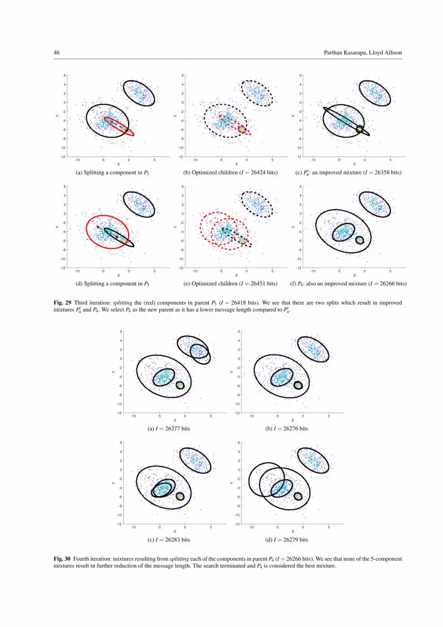
46 Parthan Kasarapu, Lloyd Allison
X
-10 -5 0 5
Y
-12
-10
-8
-6
-4
-2
0
2
4
6
(a) Splitting a component in P3
X
-10 -5 0 5
Y
-12
-10
-8
-6
-4
-2
0
2
4
6
(b) Optimized children (I = 26424 bits)X
-10 -5 0 5
Y
-12
-10
-8
-6
-4
-2
0
2
4
6
(c) P′4: an improved mixture (I = 26358 bits)
X
-10 -5 0 5
Y
-12
-10
-8
-6
-4
-2
0
2
4
6
(d) Splitting a component in P3
X
-10 -5 0 5
Y
-12
-10
-8
-6
-4
-2
0
2
4
6
(e) Optimized children (I = 26451 bits)X
-10 -5 0 5
Y
-12
-10
-8
-6
-4
-2
0
2
4
6
(f) P4: also an improved mixture (I = 26266 bits)
Fig. 29 Third iteration: splitting the (red) components in parent P3 (I = 26418 bits). We see that there are two splits which result in improvedmixtures P′4 and P4. We select P4 as the new parent as it has a lower message length compared to P′4.
X
-10 -5 0 5
Y
-12
-10
-8
-6
-4
-2
0
2
4
6
(a) I = 26277 bitsX
-10 -5 0 5
Y
-12
-10
-8
-6
-4
-2
0
2
4
6
(b) I = 26276 bits
X
-10 -5 0 5
Y
-12
-10
-8
-6
-4
-2
0
2
4
6
(c) I = 26283 bitsX
-10 -5 0 5
Y
-12
-10
-8
-6
-4
-2
0
2
4
6
(d) I = 26279 bits
Fig. 30 Fourth iteration: mixtures resulting from splitting each of the components in parent P4 (I = 26266 bits). We see that none of the 5-componentmixtures result in further reduction of the message length. The search terminated and P4 is considered the best mixture.