’’

The Journal of Problem Solving • volume 3, no. 2 (Winter 2010)1

’’

The Journal of Problem Solving • volume 4, no. 1 (Winter 2012)1

Clustering, Randomness, and Regularity: Spatial Distributions and Human Performance on the Traveling Salesperson Problem and

Minimum Spanning Tree Problem

Matthew J. Dry1, Kym Preiss2, and Johan Wagemans3

Author Note

This research was partly completed while M. Dry was a visiting research fellow at the University of Leuven and was partly supported by a grant from the University Research Council (IDO/02/004) at the University of Leuven, and from the Methusalem grant by the Flemish Government awarded to J. Wagemans (METH/08/02).

Address correspondence to: Dr Matthew J Dry, School of Psychology, University of Adelaide, Adelaide, AUSTRALIA 5005. Telephone: +618 8303 3856, Facsimile: +618 8303 3770, Email: matthew.dry@adelaide.edu.au

Abstract

We investigated human performance on the Euclidean Traveling Salesperson Problem (TSP) and Euclidean Minimum Spanning Tree Problem (MST-P) in regards to a factor that has previously received little attention within the literature: the spatial distributions of TSP and MST-P stimuli. First, we describe a method for quantifying the relative degree of clustering, randomness or regularity within point distributions. We then review evidence suggesting this factor might influence human performance on the two problem types. Following this we report an experiment in which the participants were asked to solve TSP and MST-P test stimuli that had been generated to be either highly clustered, random, or highly regular. The results indicate that for both the TSP and MST-P the participants tended to produce better quality solutions when the stimuli were highly clustered compared to random, and similarly, better quality solutions for random compared to highly regular stimuli. It is suggested that these results provide support for the ideas that human solv-ers attend to salient clusters of nodes when solving these problems, and that a similar process (or series of processes) may underlie human performance on these two tasks.

Keywords

problem solving, optimization, visual perception

1University of Adelaide; 2University of South Aulstralia;3University of Leuven

The Journal of Problem Solving •

2 Matthew J. Dry, Kym Preiss, and Johan Wagemans

It goes without saying that the human brain is an amazingly powerful data processor. At each moment it is bombarded with an astonishing array of information which it is able to analyze and interpret to generate a meaningful representation of the world, make plausible inferences and decisions, and solve a myriad of different problems, from the highly simple to the highly complex. The elegance and flexibility of this data processor is brought into acute focus by the fact that it is able to produce (seemingly effortlessly) close-to optimal solutions to problems that are computationally difficult or even intractable. One such example is the Traveling Salesman Problem.

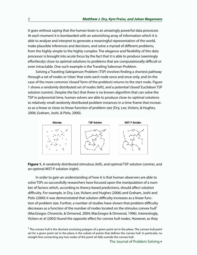
Solving a Traveling Salesperson Problem (TSP) involves finding a shortest pathway through a set of nodes or ‘cities’ that visits each node once and once only, and (in the case of the more common ‘closed’ form of the problem) returns to the start node. Figure 1 shows a randomly distributed set of nodes (left), and a potential ‘closed’ Euclidean TSP solution (centre). Despite the fact that there is no known algorithm that can solve the TSP in polynomial time, human solvers are able to produce close-to-optimal solutions to relatively small randomly distributed problem instances in a time-frame that increas-es as a linear or close-to linear function of problem size (Dry, Lee, Vickers, & Hughes, 2006; Graham, Joshi, & Pizlo, 2000).

In order to gain an understanding of how it is that human observers are able to solve TSPs so successfully researchers have focused upon the manipulation of a num-ber of factors which, according to theory-based predictions, should affect solution difficulty. For example, in Dry, Lee, Vickers and Hughes (2006) and Graham, Joshi and Pizlo (2000) it was demonstrated that solution difficulty increases as a linear func-tion of problem size. Further, a number of studies have shown that problem difficulty decreases as a function of the number of nodes located on the stimulus convex hull1 (MacGregor, Chronicle, & Ormerod, 2004; MacGregor & Ormerod, 1996). Interestingly, Vickers et al (2003) found the opposite effect for convex hull nodes. However, as they

Figure 1. A randomly distributed stimulous (left), and optimal TSP solution (centre), and an optimal MST-P solution (right).

1 The convex hull is the shortest enclosing polygon of a given point set in the plane. The convex hull point set for a given point set in the plane is the subset of points that defines the convex hull. In particular, no straight line connecting any two nodes of the point set falls outside the convex hull.

Human Performance on the Traveling Salesman and Related Problems 3

• volume 3, no. 2 (Winter 2010)

Clustering, Randomness, and Regularity 3

• volume 4, no. 1 (Winter 2012)

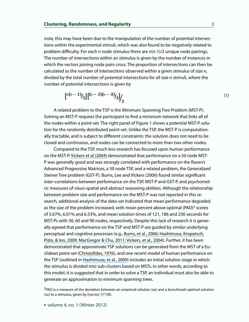
note, this may have been due to the manipulation of the number of potential intersec-tions within the experimental stimuli, which was also found to be negatively related to problem difficulty. For each n node stimulus there are n(n-1)/2 unique node pairings. The number of intersections within an stimulus is given by the number of instances in which the vectors joining node pairs cross. The proportion of intersections can then be calculated as the number of intersections observed within a given stimulus of size n, divided by the total number of potential intersections for all size n stimuli, where the number of potential intersections is given by

A related problem to the TSP is the Minimum Spanning Tree Problem (MST-P). Solving an MST-P requires the participant to find a minimum network that links all of the nodes within a point-set. The right panel of Figure 1 shows a potential MST-P solu-tion for the randomly distributed point-set. Unlike the TSP, the MST-P is computation-ally tractable, and is subject to different constraints: the solution does not need to be closed and continuous, and nodes can be connected to more than two other nodes.

Compared to the TSP, much less research has focused upon human performance on the MST-P. Vickers et al (2004) demonstrated that performance on a 50 node MST-P was generally good and was strongly correlated with performance on the Raven’s Advanced Progressive Matrices, a 50 node TSP, and a related problem, the Generalized Steiner Tree problem (GST-P). Burns, Lee and Vickers (2006) found similar significant inter-correlations between performance on the TSP, MST-P and GST-P, and psychomet-ric measures of visuo-spatial and abstract reasoning abilities. Although the relationship between problem size and performance on the MST-P was not reported in this re-search, additional analysis of the data-set indicated that mean performance degraded as the size of the problem increased, with mean percent above optimal (PAO)2 scores of 5.67%, 6.01% and 6.53%, and mean solution times of 121, 186 and 230 seconds for MST-Ps with 30, 60 and 90 nodes, respectively. Despite this lack of research it is gener-ally agreed that performance on the TSP and MST-P are guided by similar underlying perceptual and cognitive processes (e.g., Burns, et al., 2006; Haxhimusa, Kropatsch, Pizlo, & Ion, 2009; MacGregor & Chu, 2011; Vickers, et al., 2004). Further, it has been demonstrated that approximate TSP solutions can be generated from the MST of a Eu-clidean point-set (Christofides, 1976), and one recent model of human performance on the TSP (outlined in Haxhimusa, et al., 2009) includes an initial solution stage in which the stimulus is divided into sub-clusters based on MSTs. In other words, according to this model, it is suggested that in order to solve a TSP, an individual must also be able to generate an approximation to minimum spanning trees.

(1)

2PAO is a measure of the deviation between an empirical solution (se) and a benchmark optimal solution (so) to a stimulus, given by [(se/so)-1]*100.

The Journal of Problem Solving •

4 Matthew J. Dry, Kym Preiss, and Johan Wagemans

Overview

Given the general lack of research focusing upon human solutions to the MST-P, and the putative similarity of the TSP and MST-P tasks, we thought it might be useful to perform an experiment in which both tasks were performed upon a single stimulus set comprising node distributions that had been manipulated in a systematic fashion. If performance upon the two tasks were affected by the manipulation in a similar fashion, then we might be more confident that a similar process (or series of processes) under-lies these tasks.

While it would certainly be interesting to focus MST-P research upon the factors that have previously been shown to affect TSP performance, in the present study we chose to investigate a factor that has only been briefly explored in the literature: the spatial distribution of TSP and MST-P stimuli. In the following we describe a method of quantifying the degree to which stimulus nodes are alternately either distributed in clusters, are randomly distributed, or are regularly distributed. We then review theory and evidence suggesting that these alternative forms of spatial organization should affect TSP and MST-P solution difficulty. Finally we present an experiment in which we directly manipulate this factor and compare the performance of the human observers with a number of current models of human performance on TSPs and MST-Ps.

The Cluster-Random-Regular Continuum

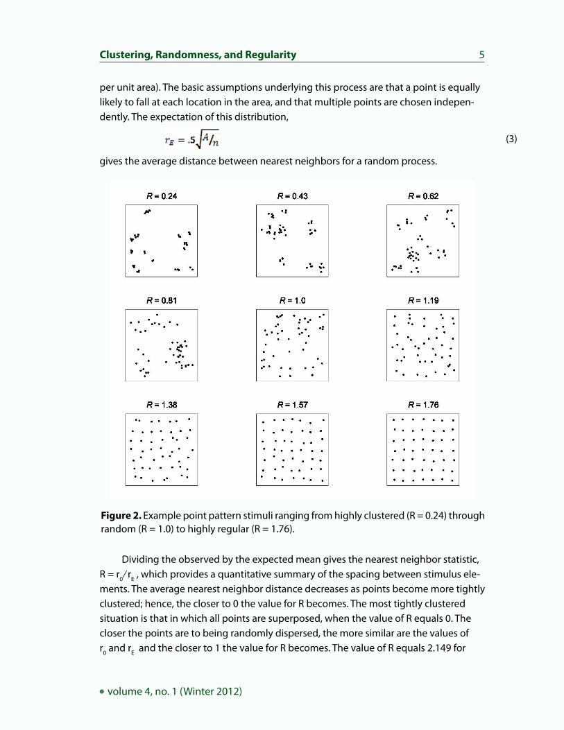
The quantification of the spatial distribution of discrete objects plays an important role in a wide range of research fields ranging from geophysics through ecology to astronomy, and numerous analytical methods have been developed towards this end (e.g., Ahuja, 1982; Aurenhammer, 1991; Boots & Getis, 1988; Clark & Evans, 1954; Gabriel & Sokal, 1969; Hertz, 1909; Ripley, 1981; Smith, 1975; Toussaint, 1980; Walford, 1951). One statistical approach that is of particular interest to the current study concerns the degree to which a given point distribution deviates from complete spatial randomness towards either clustering or regularity. Under this approach (derived independently by Clark & Evans, 1954, and Hertz, 1909), clustering, randomness and regularity are con-ceptualized as laying along a continuum, as demonstrated in Figure 2.

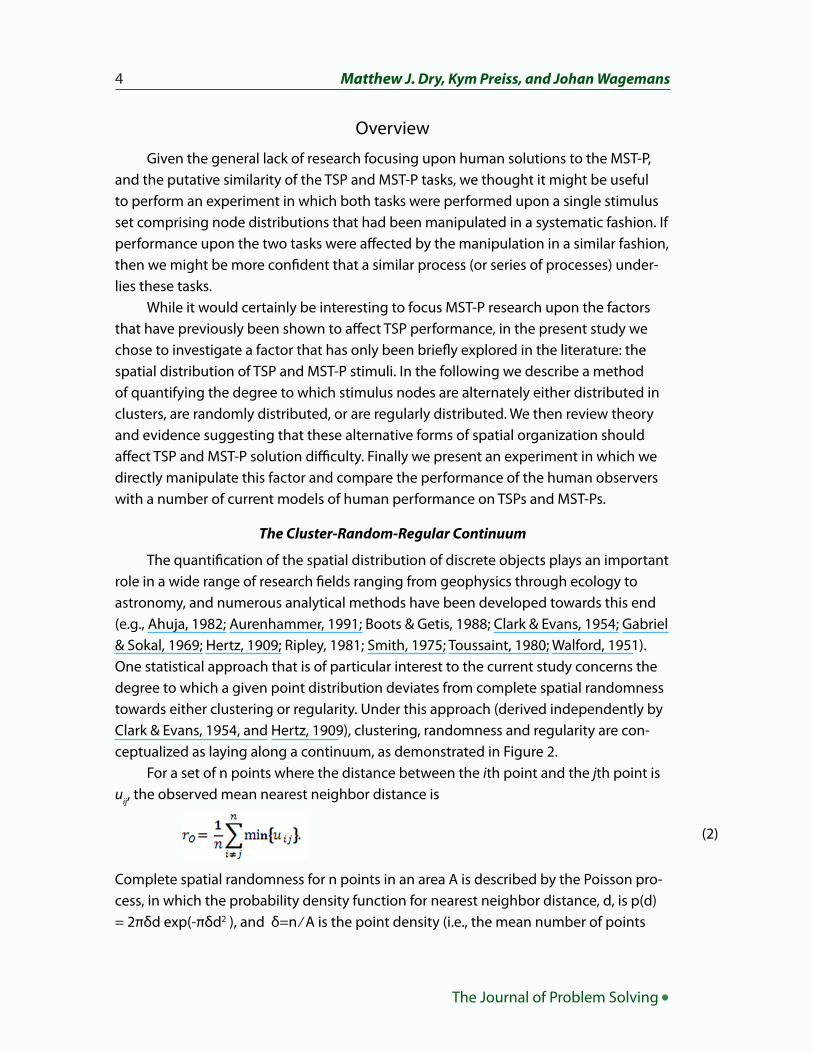
For a set of n points where the distance between the ith point and the jth point is uij, the observed mean nearest neighbor distance is

Complete spatial randomness for n points in an area A is described by the Poisson pro-cess, in which the probability density function for nearest neighbor distance, d, is p(d) = 2πδd exp(-πδd2 ), and δ=n ⁄ A is the point density (i.e., the mean number of points

(2)

Clustering, Randomness, and Regularity 5

• volume 4, no. 1 (Winter 2012)

per unit area). The basic assumptions underlying this process are that a point is equally likely to fall at each location in the area, and that multiple points are chosen indepen-dently. The expectation of this distribution,

gives the average distance between nearest neighbors for a random process.

Dividing the observed by the expected mean gives the nearest neighbor statistic, R = r0 ⁄ rE , which provides a quantitative summary of the spacing between stimulus ele-ments. The average nearest neighbor distance decreases as points become more tightly clustered; hence, the closer to 0 the value for R becomes. The most tightly clustered situation is that in which all points are superposed, when the value of R equals 0. The closer the points are to being randomly dispersed, the more similar are the values of r0 and rE and the closer to 1 the value for R becomes. The value of R equals 2.149 for

Figure 2. Example point pattern stimuli ranging from highly clustered (R = 0.24) through random (R = 1.0) to highly regular (R = 1.76).

(3)

The Journal of Problem Solving •

6 James N. MacGregor and Yun Chu

points that are spaced with perfect uniformity, as in a triangular lattice arrangement. Hence, the closer to 2.149 the value for R becomes, the more uniformly spaced are the-points. (For points located on the intersections of a square grid R = 2.)

Importantly, from a psychological point of view, research has shown that human observers are sensitive to changes in R. For example, Preiss (2006) presented 16 partici-pants with point stimuli ranging from tightly clustered (R = 0.05) to highly regular (R = 2.00) in eleven approximately equal steps. The participants were asked to rate the stim-uli on an 11 point scale ranging from “most clustered” to “most regular”, with “random” located at the midpoint of the scale. The relationship between the empirical ratings and the stimulus R was well described by a straight line, with an intercept close to zero and a slope approaching unity. Further evidence of human observers’ perceptual sensitiv-ity to changes in the relative clustering or regularity of point patterns can be found in Ginsburg and Goldstein (1987), and Allik and Tuulmets (1991).

Empirical and Theoretical Evidence

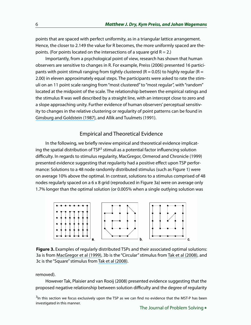
In the following, we briefly review empirical and theoretical evidence implicat-ing the spatial distribution of TSP3 stimuli as a potential factor influencing solution difficulty. In regards to stimulus regularity, MacGregor, Ormerod and Chronicle (1999) presented evidence suggesting that regularity had a positive effect upon TSP perfor-mance: Solutions to a 48 node randomly distributed stimulus (such as Figure 1) were on average 10% above the optimal. In contrast, solutions to a stimulus comprised of 48 nodes regularly spaced on a 6 x 8 grid (reproduced in Figure 3a) were on average only 1.7% longer than the optimal solution (or 0.005% when a single outlying solution was

removed).However Tak, Plaisier and van Rooij (2008) presented evidence suggesting that the

proposed negative relationship between solution difficulty and the degree of regularity

Figure 3. Examples of regularly distributed TSPs and their associated optimal solutions: 3a is from MacGregor et al (1999), 3b is the “Circular” stimulus from Tak et al (2008), and 3c is the “Square” stimulus from Tak et al (2008).

3In this section we focus exclusively upon the TSP as we can find no evidence that the MST-P has been investigated in this manner.

The Journal of Problem Solving •

6 Matthew J. Dry, Kym Preiss, and Johan Wagemans

Clustering, Randomness, and Regularity 7

• volume 4, no. 1 (Winter 2012)

in the distribution of stimulus nodes may be attenuated by the degree of regularity and symmetry in the optimal solution. They presented participants with regularly distrib-uted stimuli for which the optimal solution was asymmetrical. For the 21 node ‘Circular’ stimulus (reproduced in Figure 3b) the average deviation from optimal was 6.53%, well above the 2.51% we could expect for randomly distributed 20 node point-sets (Dry et al., 2006). For the ‘Square’ stimulus (reproduced in Figure 3c) the average deviation from optimal was 4.29% which is within the range of the expected value of 4.11% for 25 node point-sets (obtained by linearly extrapolating between the mean scores for 20 and 30 node problems in Dry, et al., 2006). In other words, it would appear that stimulus regularity does not necessarily lead to an improvement in TSP performance.

In regards to stimulus clustering, we are aware of only a single study involving TSPs (Hirtle & Gärling, 1992) in which this factor has been specifically manipulated. In this study the participants were presented with stimuli that were comprised of either clusters of nodes or randomly distributed nodes, with the general pattern of results in-dicating that clustering enhanced the quality of the empirical solutions. As MacGregor and Chu (2011) note such an outcome is consistent with the idea that the human visual system may be employing some form of clustering heuristic when generating TSP solu-tions. The potential importance of the perception of salient clusters when generating solutions to TSPs was suggested as early as (what is generally regarded as) the first study examining human performance on TSPs (Polianova, 1974), and has been a feature of numerous theoretical and computational accounts of human performance in subse-quent studies. For example, Vickers, Lee Dry and Hughes (2003) proposed a potential model of human performance on TSPs, the Hierarchical Nearest Neighbor (HNN) model. According to this model observers solve TSPs by initially forming sub-clusters of stimu-lus nodes based on nearest neighbor distances, which are then sequentially linked to form a tour. Similarly, the Hierarchical Pyramid (HP) model (Graham, et al., 2000; Hax-himusa, et al., 2009; Pizlo et al., 2006) operates by forming initial sub-clusters of nodes, and clusters of sub-clusters in an iterative fashion until there are only three or four clusters represented in the problem space. The model then generates a tour by working down through the cluster hierarchy, thereby creating increasingly finer-grained tours, until the pathway is located at the level of the stimulus nodes. The model outlined in Kong, Schunn and Waalstrom (2007) also employs a coarse-to-fine method of tour gen-eration based on an initial representation comprised of node clusters generated via a k-means clustering algorithm.

In the case of both the TSP and MST-P it is reasonable to assume that stimuli which contain salient sub-clusters should precipitate the formation of the initial represen-tational space. Conversely, highly regular (but not perfectly regular and symmetrical) stimuli (in which there few salient sub-clusters) should theoretically be more difficult to solve. Further, if the observers are able to form a cluster-based representation, then

The Journal of Problem Solving •

8 James N. MacGregor and Yun Chu

a TSP or MST-P of size N becomes (in effect) a problem of size k (where N is the number of nodes and k is the number of clusters). We should therefore expect that the degree of clustering in a stimulus should also affect the amount of time taken to solve the two classes of problem.

In the following we present an experiment in which the test stimuli comprised point distributions ranging from highly clustered, through random, to highly regular. The participants were asked to solve the stimuli as either TSPs, or MST-Ps.

Method

Participants

There were 58 participants, with a mean age of 24. All of the participants were currently studying at the University of Adelaide. They were paid the equivalent of $15 AUS for participating in the experiment. Ethics approval was obtained from the University of Adelaide School of Psychology human ethics subcommittee.

Stimuli

All of the stimuli were presented on a uniform white background within a 19cm x 19cm square located at the centre of the screen on a 1280 by 1028 pixel color computer mon-itor with a refresh rate of 85 Hz. The nodes were black circles with a 3 mm diameter, and were constrained to be at least 3mm apart.

In order to test a range of stimulus spatial organization levels we chose target R-values of 0.62, 1.00 and 1.38 (corresponding to clustered, random and regular stimuli, respectively). Examples of test stimuli with these R-values are shown along the top-right to bottom-left diagonal in Figure 2. For each target R-value we generated a pool of 10,000 stimuli with 49 nodes. For the clustered stimuli we initially generated clus-ters containing 2 to 5 nodes. The initial clusters were randomly distributed across the stimulus, but all of the nodes within a cluster were (to begin with) located at the same spatial location. For the regular stimuli we initially generated stimuli in which the nodes were uniformly distributed in a 7x7 grid. For each of these two stimulus classes we then added random spatial ‘jitter’ to the nodes until the desired R-value was reached. For the random stimuli the spatial location of the nodes was determined via a standard ran-dom number generator. All of the stimuli were within a tolerance range of +/- 0.001 of the target R-value.

As described earlier, two factors that have been shown have a significant impact on performance upon TSPs are the number of potential intersections within a stimulus and the number of nodes located on the convex hull. In regards to the first factor the data indicated that the number of potential intersections increased as a function of R,

8 Matthew J. Dry, Kym Preiss, and Johan Wagemans

The Journal of Problem Solving •

Clustering,Randomness, and Regularity 9

• volume 4, no. 1 (Winter 2012)

with a mean of 0.228, 0.232 and 0.233 for the clustered, random and regular stimuli, re-spectively. In order to control for this we discarded any stimuli with a number of poten-tial intersections outside of the range .232 +/- 0.0001. From the remaining stimuli we chose 5 stimuli from each of the 3 stimulus classes such that the number of nodes on the convex hull was close to equal. The mean number of nodes on the convex hull was 11, 11, and 11.2 for the clustered, random and regular stimuli, respectively.

Procedure

The participants were randomly assigned to one of three conditions: a TSP condition, a MST-P condition and a tracing condition.

The TSP and MST-P conditions were each completed by 25 participants. Partici-pants in the TSP condition solved the stimuli as TSPs only and vice versa for the MST-P condition. The participants were presented with the same stimulus set regardless of whether they were in the TSP or MST-P condition. The only procedural difference be-tween the two conditions related to the instructions given for producing solutions to the TSP or MST-P.

The participants could create solutions by using the mouse to click on pairs of nodes, resulting in a red line joining the node-pair. At any stage the participants could remove any link by clicking on the associated node-pair. The participants were instruct-ed that they were free to start at any node, to connect the nodes in any order, and to work on separate clusters on nodes at the same time. No time limit was placed upon the time taken to complete a solution.

Each participant completed all 15 stimuli, and the stimuli were presented in a dif-ferent random order for each participant. Immediately prior to the experiment the par-ticipants completed a single practice stimulus.

The remaining 8 participants took part in the tracing condition. As noted in Dry et al (2006) the time taken for a participant to complete a TSP (or MST-P) comprises both cognitive and motor components. By subtracting the motor component from the overall solution time we are able to obtain a measure of the time taken to perform the cognitive decision-making component of the task. Such an approach is potentially important for two reasons. First, the experimental manipulation of the stimulus point distributions may lead to differences in the time taken to physically complete the solu-tions. Specifically, the inter-node distances of the regularly distributed stimuli will be, on average, greater than those of the other stimuli classes. This may cause an increase in overall solution time that is due to the motor component of the task rather than the, arguably more interesting, cognitive component. Second, the different requirements of the TSP and MST-P tasks may also lead to differences in overall solution time caused by the time taken to physically complete the tasks, making it difficult to make compari-

The Journal of Problem Solving •

10 James N. MacGregor and Yun Chu

sons across the two tasks with regard to relative cognitive complexity.The stimuli employed in the tracing condition were the same as those in the other

two conditions, with the exception that the nodes were overlaid with either an MST-P or TSP solution. The overlaid solutions were drawn from the empirical solutions gener-ated by the participants in the TSP and MST-P conditions, and were, in each case, the empirical solution that was closest to the mean PAO for each stimulus.

The participants in the tracing condition were instructed to trace the solution displayed on the screen as quickly as possible, without taking a break until the entire solution was traced. The participants traced the solutions using the same procedure as in the TSP and MST-P conditions, i.e., by using the mouse to click on pairs of nodes and create a link between them. The participants were presented with all 15 stimuli in a ran-domized order. Half of the participants followed the TSP solutions first followed by the MST-P solutions. The remaining participants completed the task in the opposite order.

Results

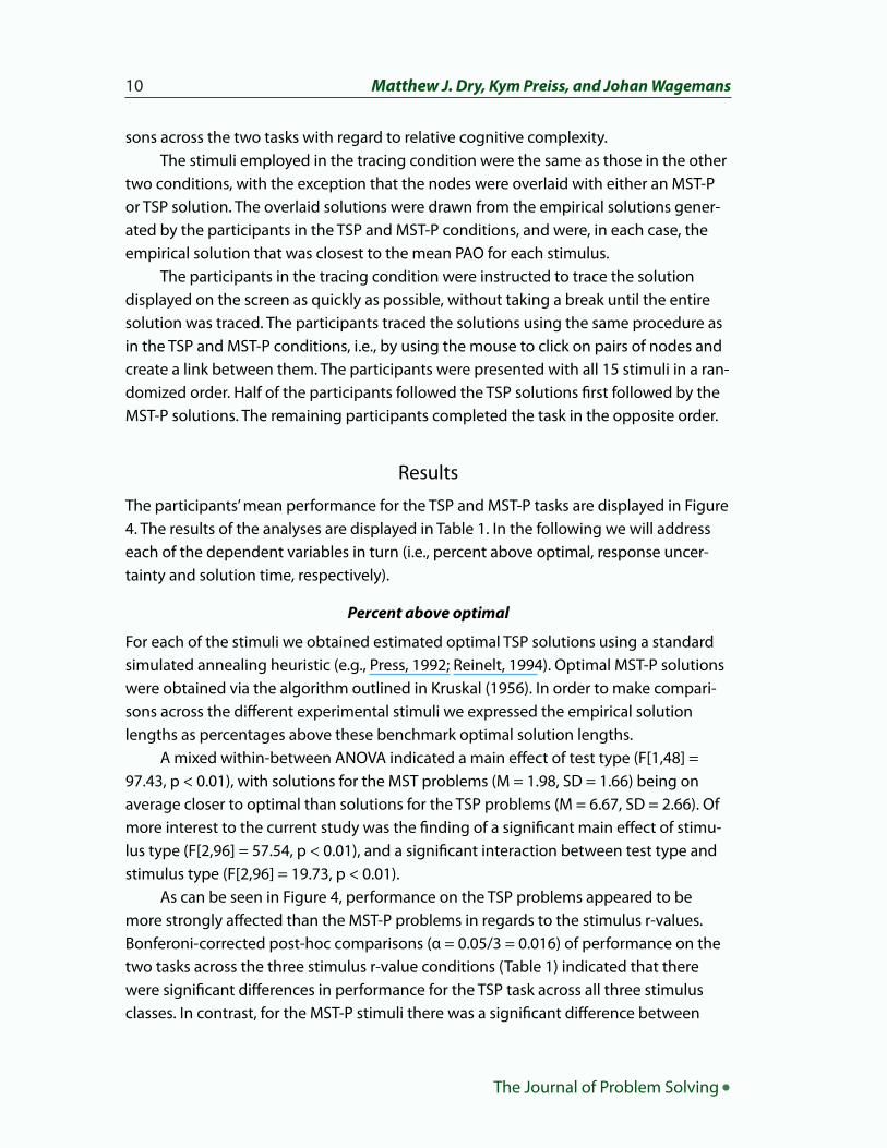
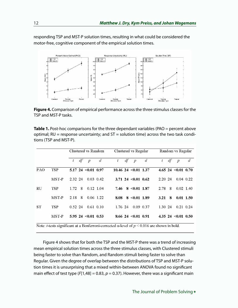
The participants’ mean performance for the TSP and MST-P tasks are displayed in Figure 4. The results of the analyses are displayed in Table 1. In the following we will address each of the dependent variables in turn (i.e., percent above optimal, response uncer-tainty and solution time, respectively).

Percent above optimal

For each of the stimuli we obtained estimated optimal TSP solutions using a standard simulated annealing heuristic (e.g., Press, 1992; Reinelt, 1994). Optimal MST-P solutions were obtained via the algorithm outlined in Kruskal (1956). In order to make compari-sons across the different experimental stimuli we expressed the empirical solution lengths as percentages above these benchmark optimal solution lengths.

A mixed within-between ANOVA indicated a main effect of test type (F[1,48] = 97.43, p < 0.01), with solutions for the MST problems (M = 1.98, SD = 1.66) being on average closer to optimal than solutions for the TSP problems (M = 6.67, SD = 2.66). Of more interest to the current study was the finding of a significant main effect of stimu-lus type (F[2,96] = 57.54, p < 0.01), and a significant interaction between test type and stimulus type (F[2,96] = 19.73, p < 0.01).

As can be seen in Figure 4, performance on the TSP problems appeared to be more strongly affected than the MST-P problems in regards to the stimulus r-values. Bonferoni-corrected post-hoc comparisons (α = 0.05/3 = 0.016) of performance on the two tasks across the three stimulus r-value conditions (Table 1) indicated that there were significant differences in performance for the TSP task across all three stimulus classes. In contrast, for the MST-P stimuli there was a significant difference between

10 Matthew J. Dry, Kym Preiss, and Johan Wagemans

The Journal of Problem Solving •

Clustering, Randomness, and Regularity 11

• volume 4, no. 1 (Winter 2012)

performance on the Clustered and Regular stimuli, but not the Clustered and Random, or Random and Regular stimuli.

Response Uncertainty

Response uncertainty (RU) is a measure of the degree of agreement in the solutions constructed by the participants for each of the stimuli. We calculated response uncer-tainty using Shannon’s (1949) standard information theory formula

where pi indicates the probability of a given inter-node link i being chosen by the par-ticipants.

Independent samples ANOVA indicated a main effect of test type (F[1,24] = 375.64, p < 0.01) and a main effect of stimulus type (F[2,24] = 28.66, p < 0.01), but no significant interaction (F[2,24] = 0.60, p =0.56). As can be seen in Figure 4, performance on both the TSP and MST-P appeared to be strongly affected by the stimulus R-values, with the degree of agreement in the participants’ solutions decreasing as a function of increasing R. Despite this, Bonferroni-corrected post-hoc comparisons (Table 1) indi-cated that for the TSP task there was a significant difference between the clustered and regular stimuli, but not the clustered and random stimuli, or the random and regular stimuli. For the MST-P task there was a significant difference between the clustered and regular stimuli, and the random and regular stimuli, but not the clustered and random stimuli (Table 1). It should be noted that if we employed a less conservative α-level (e.g., 0.05 rather than 0.016) the pattern of significant differences indicated by the post-hoc comparisons would be identical for the TSP and MST-P tasks, thereby explaining the lack of a significant interaction effect in the ANOVA.

It should also be noted that for both the TSP and MST-P the associated effect sizes (Cohen’s d; see Table 1) indicate that the distributions of RU values are at least 1.03stan-dard deviations apart, regardless of the significance of the post-hoc comparisons. Hence, it is reasonable to assume that if we had included a greater number of stimuli in the test-set then each of these comparisons would have been significant at the Bonfer-roni-corrected α-level of 0.016.

Solution Time

In order to obtain a motor-free measure of solution time we first averaged across the empirical tracing times obtained in the solution tracing condition, resulting in values of 48.03, 52.82, and 50.89 seconds for the clustered, random and regular TSP solutions respectively, and 56.91, 58.92, and 66.37 seconds for the clustered, random and regular MST-P solutions respectively. We then subtracted these values from the cor-

(4)

The Journal of Problem Solving •

12 James N. MacGregor and Yun Chu

responding TSP and MST-P solution times, resulting in what could be considered the motor-free, cognitive component of the empirical solution times.

Figure 4 shows that for both the TSP and the MST-P there was a trend of increasing mean empirical solution times across the three stimulus classes, with Clustered stimuli being faster to solve than Random, and Random stimuli being faster to solve than Regular. Given the degree of overlap between the distributions of TSP and MST-P solu-tion times it is unsurprising that a mixed within-between ANOVA found no significant main effect of test type (F[1,48] = 0.83, p = 0.37). However, there was a significant main

Figure 4. Comparison of empirical performance across the three stimulus classes for the TSP and MST-P tasks.

Table 1. Post-hoc comparisons for the three dependant variables (PAO = percent above optimal; RU = response uncertainty; and ST = solution time) across the two task condi-tions (TSP and MST-P).

12 Matthew J. Dry, Kym Preiss, and Johan Wagemans

The Journal of Problem Solving •

Clustering, Randomness, and Regularity 13

• volume 4, no. 1 (Winter 2012

effect of stimulus class (F[2,96] = 19.76, p < 0.01), and a significant interaction between test type and stimulus class (F[2,96] = 4.76, p = 0.01). Post-hoc comparisons (Table 1) indicated that there were no significant differences between the TSP solution times across the three stimulus classes, but the MST-P solution times for the clustered stimuli were significantly shorter than those for the random and regular stimuli, and the solu-tion times for the random stimuli were significantly shorter than those for the regular stimuli.

In order to determine if the results of the solution time data analyses arose as a re-sult of the removal of the tracing times from the overall solution times we ran addition-al analyses based on the raw solution time data. In the case of both the TSP and MST-P solutions times the overall pattern of results was identical to those reported above.

Discussion

The results of the experiment indicate that human solutions to the TSP and MST-P are affected by the spatial distribution of the stimuli in a qualitatively similar fashion, with performance progressively degrading as the stimulus R-values shift from highly clus-tered, through random, to highly regular. It would appear that for both problem types the presence of salient sub-clusters within a stimulus leads to better solutions, less variability across the participants’ solutions, and reduced solution times, providing em-pirical support for the suggestion that human solvers may be employing some form of clustering heuristic when producing solutions to these problems.

While the overall effect of manipulating the spatial distributions of the stimuli was similar for both tasks, the results also point to some interesting differences between them. As was indicated in the results section, the participants in the TSP condition pro-duced solutions that deviated further from the optimal solution compared to the par-ticipants in the MST-P condition, and there was a higher degree of variability in the TSP solutions (as measured by RU) compared to the MST-P solutions. Such a result is broad-ly consistent with the difference between the two tasks in regards to computational complexity: Unlike the TSP, the MST-P can be solved algorithmically in polynomial time. Hence, it is unsurprising that the TSP should be a more difficult task than the MST-P.

Given these apparent differences in computational complexity, it is somewhat surprising that the results indicate that there was no significant difference in the time taken by the participants to solve the two tasks. One potential explanation may be that the solution time data is inherently ‘noisy’ as evinced by the relative widths of the error-bars in Figure 4. In light of this it is reasonable to assume that any difference between the two tasks, if there was indeed a difference to be found, would be harder to find in the solution time data compared to the other dependent variables. Nonetheless, while it is relatively easy to imagine that the addition of further data-points may reduce the

The Journal of Problem Solving •

14 James N. MacGregor and Yun Chu

variance in the distributions, the notion that this process might also lead to a swapping of the order of the distributions (such that the TSP takes longer to solve than the MST-P) seems less likely.

Further, it is not clear why there should be a significant effect of stimulus class upon solution times for the MST-P but not for the TSP. Again, we can only speculate in regards to this matter, but it could be that this is due to differences in the task demands of the two problem types. For example, let us assume that participants form an initial solution state for either task by segmenting the stimulus into salient clusters of nodes. For the MST-P a solution could then be generated by simply joining these clusters up into a single spanning tree. It is reasonable to assume that the choice of appropriate inter-cluster links would be easier in the case of the clustered stimuli compared to the regular stimuli, leading to longer solution times for the latter class of stimuli. In regards to the TSP, moving from the initial clustering state to a finished solution is an arguably more complex process, requiring the clusters to be joined into a single, continuous loop. It is possible that this added complexity leads to something of a ceiling effect that swamps any potential effect of differences in the spatial distributions of the stimuli.

Speculation aside, the results of this experiment are potentially informative for any models of human performance on these tasks. Specifically, they suggest that any plau-sible model should take into account the effects of the spatial distributions of the stim-uli, and reflect the same ordering of solution difficulty as given by the empirical data. While a formal comparison of extant models is beyond the scope of this paper, it would be interesting to determine whether models such as the hierarchical pyramid model (e.g., Graham, et al., 2000; Haxhimusa et al., 2011; Haxhimusa, et al., 2009; Pizlo, et al., 2006) and the k-means model (Kong & Schunn, 2007), which include a specific cluster-ing stage in the solution process, are able to provide a better account of the empirical data than models such as the sequential convex hull model (MacGregor, Ormerod, & Chronicle, 2000), which do not.

Finally, it is worthwhile noting that some of the participants appeared to be ac-tively aware of the relative difference in difficulty between the stimulus classes despite the fact that they were not given any feedback regarding their performance during the course of the experiment. Once they had completed the experiment a number of the participants made un-prompted comments regarding the task, noting that certain stimuli felt easier to solve than others. When asked if they could pinpoint any particular factor that could differentiate the ‘hard’ and ‘easy’ stimuli many noted that the problems comprised of nodes ‘bunched’ or ‘grouped together’ were easier to solve than the stim-uli that were ‘spread out’. Of course this information is anecdotal, but it adds support to the findings of Preiss (2006) that observers are sensitive to differences in the spatial dis-tributions of the point-patterns. It would be interesting to determine if the participants made the association between relative difficulty and stimulus class once they had com-

14 Matthew J. Dry, Kym Preiss, and Johan Wagemans

The Journal of Problem Solving •

Clustering,Randomness, and Regularity 15

• volume 4, no. 1 (Winter 2012)

pleted some or all of the problems, or whether these associations arose spontaneously and instinctively upon first viewing each of the problems.

In summary, the results of the current experiment have added to our understand-ing of the factors which affect human performance on the TSP, and a related problem, the MST-P. Along with problem size, number of nodes on the convex hull and number of potential intersections, the relative difficulty of solving these tasks is also affected by the spatial distributions of the stimuli. Specifically, the more clustered a stimulus is, the easier it is to solve. Furthermore, the similarity of the effects of manipulating this factor upon the two tasks provides empirical support for the suggestion that human solutions to the TSP and MST-P are generated by a related process or series of processes. Finally, it seems reasonable to suggest that any plausible model of human performance on these tasks should reflect the same sensitivity to the manipulation of this factor as that shown by the empirical data.

ReferencesAhuja, N. (1982). Dot pattern processing using Voronoi neighborhoods. IEEE Transactions

on Pattern Analysis and Machine Intelligence, 4(3), 336-343.

Allik, J., & Tuulmets, T. (1991). Occupancy model of perceived numerosity. Perception & Psychophysics, 49, 303-314.

Aurenhammer, F. (1991). Voronoi diagrams - A survey of a fundamental geometric data structure. ACM Computing Surveys, 23(3), 345-405.

Boots, B. N., & Getis, A. (Eds.). (1988). Point pattern analysis Volume 8: Sage Publications.

Burns, N. R., Lee, M. D., & Vickers, D. (2006). Are individual differences in performance on perceptual and cognitive optimization problems determined by general intelligence? The Journal of Problem Solving, 1(5-19).

Christofides, N. (1976). Worst-case analysis of a new heuristic for the travelling salesman problem: Report 388, Graduate School of Industrial Administration, CMU.

Clark, P. J., & Evans, F. C. (1954). Distance to nearest neighbor as a measure of spatial rela-tionships in populations. Ecology, 35, 445-453.

Dry, M. J., Lee, M. D., Vickers, D., & Hughes, P. (2006). Human performance on visually pre-sented traveling salesperson problems with varying numbers of nodes. The Journal of Problem Solving, 1, 20-32.

Gabriel, K. R., & Sokal, R. R. (1969). A new statistical approach to geographic variation analysis. Systematic Zoology, 18, 259-278.

Ginsburg, N., & Goldstein, S. R. (1987). Measurement of visual cluster. American Journal Of Psychology, 100, 193-203.

Graham, S. M., Joshi, A., & Pizlo, Z. (2000). The traveling salesman problem: A hierarchical model. Memory & Cognition, 28(7), 1191-1204.

The Journal of Problem Solving •

16 James N. MacGregor and Yun Chu

Haxhimusa, Y., Carpenter, E., Catrambone, J., Foldes, D., Stefanov, E., Arns, L., et al. (2011). 2D and 3D traveling salesman problem. The Journal of Problem Solving, 3, 167-193.

Haxhimusa, Y., Kropatsch, W. G., Pizlo, Z., & Ion, A. (2009). Approximate graph pyramid solution of the E-TSP. Image and Vision Computing, 27, 887-896.

Hertz, P. (1909). Uber den geigenseitigen durchschnittlichen Abstand von Punkten, die mit bekannter mittlerer Dichte im Raume angeordnet sind. Mathematische Annalen, 67, 387-398.

Hirtle, D. C., & Gärling, T. (1992). Heuristic rules for sequential spatial decision makers. Geoforum, 23, 227-238.

Kong, X., & Schunn, C. D. (2007). Global vs. local information processing in visual/spatial problem solving: The case of the traveling salesman problem. Cognitive Systems Research, 8, 192-207.

Kruskal, J. B. (1956). On the shortest spanning subtree of a graph and the traveling sales-man problem. Proceedings of the American Mathematical Society, 7, 48-50.

MacGregor, J. N., Chronicle, E. P., & Ormerod, T. C. (2004). Convex hull or crossing avoid-ance? Solution heuristics in the traveling salesperson problem. Memory & Cognition, 32, 260-270.

MacGregor, J. N., & Chu, Y. (2011). Human performance on the traveling salesman and related problems: A review. The Journal of Problem Solving, 3, 1-29.

MacGregor, J. N., & Ormerod, T. C. (1996). Human performance on the traveling salesman problem. Perception & Psychophysics, 58, 527-539.

MacGregor, J. N., Ormerod, T. C., & Chronicle, E. P. (1999). Spatial and contextual factors in human performance on the travelling salesperson problem. Perception, 28, 1417-1427.

MacGregor, J. N., Ormerod, T. C., & Chronicle, E. P. (2000). A model of human performance on the traveling salesperson problem. Memory & Cognition, 28, 1183-1190.

Ormerod, T. C., & Chronicle, E. P. (1999). Global perceptual processing in problem solving: The case of the traveling salesperson. Perception & Psychophysics, 61, 1227-1238.

Pizlo, Z., Stefanov, E., Saalweachter, J., Li, Z., Haxhimusa, Y., & Kropatsch, W. G. (2006). Traveling salesperson problem: A foveating pyramid model. The Journal of Problem Solving, 1, 83-101.

Polianova, N. I. (1974). On some functional and structural features of the visual-intuitive components of a problem-solving process. Voprosy Psikhologii, 4, 41-51.

Preiss, K. (2006). A theoretical and computational investigation into aspects of human visual perception: Proximity and transformations in pattern detection and discrimination. Un-published Ph.D, University of Adelaide, Adelaide.

Press, W. H. (1992). Numerical recipes in FORTRAN: The art of scientific computing. (2nd ed.). Cambridge: Cambridge University Press.

Reinelt, G. (1994). The travelling salesman: Computational solutions for TSP applications Lecture notes in computer science (Vol. 840). Berlin: Springer-Verlag.

16 Matthew J. Dry, Kym Preiss, and Johan Wagemans

The Journal of Problem Solving •

Clustering, Randomness, and Regularity 17

• volume 4, no. 1 (Winter 2012)

Ripley, B. D. (1981). Spatial statistics. New York: John Wiley & Sons.

Shannon, C. E., & Weaver, W. (1949). The mathematical theory of communication. Urbana, IL: University of Illinois Press.

Smith, D. M. (1975). Patterns in human geography: An introduction to numerical methods. New York: Crane, Russak & Company.

Tak, S., Plaiser, M., & van Rooij, I. (2008). Some tours are more equal than others: The con-vex hull model revisited with lessons for testing models of the traveling salesperson problem. The Journal of Problem Solving, 2, 4-28.

Toussaint, G. T. (1980). The relative neighborhood graph of a finite planar set. Pattern Recognition, 12(4), 261-268.

Vickers, D., Lee, M. D., Dry, M. J., & Hughes, P. (2003). The roles of the convex hull and the number of potential intersections in performance on visually presented traveling salesperson problems. Memory & Cognition, 31, 1094-1104.

Vickers, D., Mayo, T., Heitmann, M., Lee, M., & Hughes, P. (2004). Intelligence and individual differences in performance on three types of visually presented optimisation prob-lems. Personality and Individual Differences, 36, 1059-1071.

Walford, N. (1951). Geographical data analysis. Chichester, New York: John Wiley & Sons.