boussinesq modeling of surface waves due to underwater landslides

arX

iv:1

112.

5083

v1 [

phys

ics.

clas

s-ph

] 2

1 D

ec 2

011

BOUSSINESQ MODELING OF SURFACE WAVES DUE TO

UNDERWATER LANDSLIDES

DENYS DUTYKH AND HENRIK KALISCH∗

Abstract. Consideration is given to the influence of an underwater landslide

on waves at the surface of a shallow body of fluid. The equations of motion

which govern the evolution of the barycenter of the landslide mass include var-

ious dissipative effects due to bottom friction, internal energy dissipation, and

viscous drag. The surface waves are studied in the Boussinesq scaling, with

time-dependent bathymetry. A numerical model for the Boussinesq equations

is introduced which is able to handle time-dependent bottom topography, and

the equations of motion for the landslide and surface waves are solved simulta-

neously.

The numerical solver for the Boussinesq equations can also be restricted to

implement a shallow-water solver, and the shallow-water and Boussinesq con-

figurations are compared. A particular bathymetry is chosen to illustrate the

general method, and it is found that the Boussinesq system predicts larger wave

run-up than the shallow-water theory in the example treated in this paper. It

also found that the finite fluid domain has a significant impact on the behaviour

of the wave run-up.

PACS classification: 45.20.D,47.11.Df, 47.35.Bb, 47.35.Fg, 47.85.Dh.

Contents

1. Introduction 22. The landslide model 43. The Boussinesq model 84. Solitary waves 105. The numerical scheme 125.1. High-order reconstruction 145.2. Treatment of the dispersive terms 155.3. Time stepping 165.4. Validation 176. Numerical results and discussion 177. Conclusion 24Acknowledgements 24References 24

Key words and phrases. Surface waves; Boussinesq model; submarine landslides; wave run-up;

tsunami.∗ Corresponding author.

1

http://arxiv.org/abs/1112.5083v1

2 D. DUTYKH AND H. KALISCH

1. Introduction

Surface waves originating from sudden perturbations of the bottom topographyare often termed tsunamis. Two distinct generation mechanisms of a tsunami areunderwater earthquakes, and submarine mass failures. Among the broad class ofsubmarine mass failures, landslides can be characterized as translational failureswhich travel considerable distances along the bottom profile [27, 41]. In the past,the role of landslides and rock falls in the excitation of tsunamis may have beenunderestimated, as most known occurrences of tsunamis were accredited to seismicactivity. However, it is now more accepted that submarine mass failures alsocontribute to a large portion of tsunamis [47]. Recent years have seen a multitudeof works devoted to the study of such underwater landslides and the resulting effecton surface waves. A sample of results which are available can be found in [2, 11,13, 19, 26, 27, 35, 36, 40, 47]. Of course this list is far from exhaustive. It shouldalso be mentioned that it is possible for underwater landslides and earthquakes toact in tandem, producing very large surface waves [21].

A natural question to ask is whether the effect on surface waves can be suchthat they may pose a danger for civil engineering structures located near the shore.Consequently, one important issue is the wave action and in particular the run-upand draw-down at beaches in the vicinity of the landslide. While the draw-downitself may not pose a threat, one consequence of a large draw-down can be theamplification of the run-up of the following positive wave crest [16, 45].

There have been many numerical and a few experimental studies devoted to thissubject, but it is generally difficult to include many of the complex parametersand dependencies of a realistic landslide into a physical model. Therefore, mostworkers attempt to distill the problem to a model setup where many effects suchas turbulence and sedimentation are disregarded.

For example, Grilli and Watts study tsunami sensitivity to several landslideparameters in the case of a landslide in a coastal area of an open ocean [27]. Inparticular, dependence on the landslide shape and the initial depth of the landslidelocation are studied, and it is found that the landslide with the smallest lengthproduced the largest waveheight and run-up, and that the wave run-up at an adja-cent beach is inversely proportional to the initial depth. The work in [27] relies onintegrating the full water-wave equations using an irrotational boundary-elementcode, and using an open boundary with transmission conditions [25, 24]. Whilemost works have considered a given dynamics for the landslide, the bottom motionin [27] is described by an ordinary differential equation similar to the one used here.Thus the motion of the landslide is computed using a differential equation derivedfrom first principles using Newtonian mechanics. However to expedite comparisonwith experiments, the landslide in [27] is considered moving on a straight inclinedbottom with constant slope.

More recently, Khakimzyanov and Shokina [32], and Chubarov et. al. [11] havealso used a differential equation to find the bottom motion. One major novelty in

MODELING OF SURFACE WAVES DUE TO UNDERWATER LANDSLIDES 3

their work is that the landslide motion is computed on a bottom with an arbitraryshape. The time-dependent bathymetry is then used to drive a numerical solver ofthe shallow-water equations. An advantage of this approach when compared to [27]is the reduced computation time. On the other hand, the description of the wavemotion in the shallow-water theory is only approximate, and in particular, oneimportant effect of surface waves, namely the influence of dispersion is neglected.

The main aim of the current work is to introduce the effect of dispersion intothe description of the wave motion at the surface of the fluid while keeping thesimplicity of the shallow-water approach. To this end, we utilize the so-calledPeregrine system which is a particular case of a general class of model systemswhich arise in the Boussinesq scaling [9]. A common feature of all Boussinesq-type systems is that they allow a simplified study of surface waves in which bothnonlinear and dispersive effects are taken into account. In the present case, weneed to use a Boussinesq system which can handle complex and time-dependentbottom topography. Such a system was derived by Wu [52], and can be used inconnection with the dynamic bathymetry.

We conduct two main experiments. First, a comparison with the shallow-watertheory is carried out. Second, the dependence of the tsunami characteristics on theinitial depth of the landslide is investigated. The main findings of the present workare that the predictions of the shallow-water and Boussinesq theory are divergentfor the cases treated in this paper, and that the effect of a finite fluid domain,such as a river, lake or fjord [40] can lead to significantly different behaviour whencompared to tsunamis on an open ocean.

The Boussinesq model in this paper is based on the assumption of an inviscidfluid, and irrotational flow. These are standard assumptions in the study of surfacewaves, and generally give good results, unless there are strong background currentsin the fluid. Another effect which is not taken account of here is the wave resistanceon the landslide due to waves created by the motion of the landslide. However,as observed in [29], this effect is negligible for most realistic cases of underwaterlandslides. Viscosity is included in the dynamic model for the landslide as willbe shown in the next section. In order to capture the effect of slide deformationduring the evolution, a damping term in the equation of motion is included tomodel the internal friction in the landslide mass.

The paper is organized in the following way. In Section 2, the equation of motionfor the landslide is developed. Then in Section 3, the Boussinesq model is recalled.In Section 4, solitary-wave solutions of the Peregrine system are found numerically.In Section 5, the numerical scheme for the Boussinesq system is explained andthe numerical method is tested using the exact solutions of Section 4. Section 6contains results of numerical runs for a few specific cases of bottom bathymetry,a parameter study of wave run-up in relation to the initial depth of the landslide,and a comparison with the shallow-water theory.


0 20 40 60 80 100 120−20

−15

−10

−5

0

x

z

Bathymetry and landslide position at t = 50 s

LandslideSolid bottom

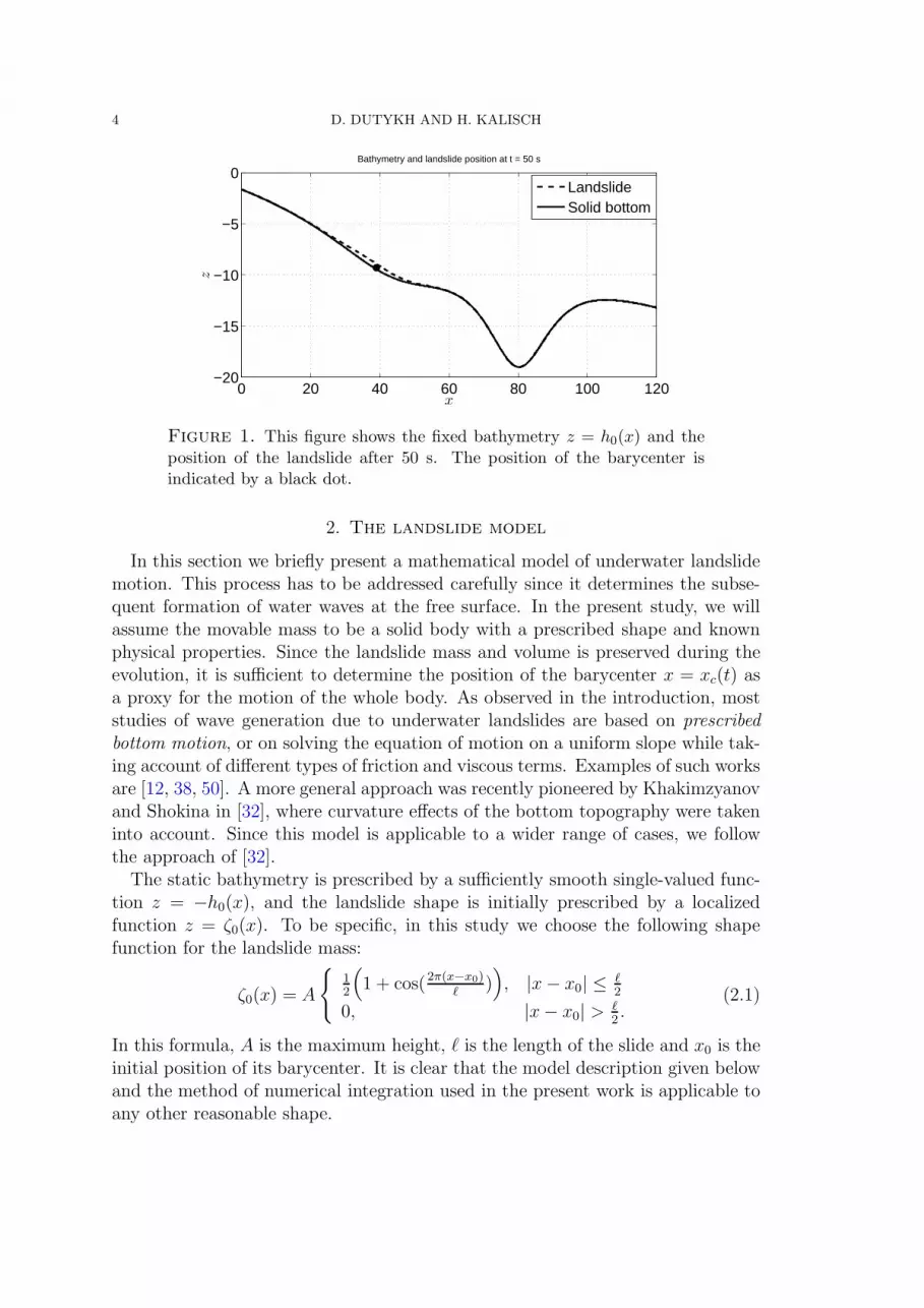
Figure 1. This figure shows the fixed bathymetry z = h0(x) and the

position of the landslide after 50 s. The position of the barycenter isindicated by a black dot.

2. The landslide model

In this section we briefly present a mathematical model of underwater landslidemotion. This process has to be addressed carefully since it determines the subse-quent formation of water waves at the free surface. In the present study, we willassume the movable mass to be a solid body with a prescribed shape and knownphysical properties. Since the landslide mass and volume is preserved during theevolution, it is sufficient to determine the position of the barycenter x = xc(t) asa proxy for the motion of the whole body. As observed in the introduction, moststudies of wave generation due to underwater landslides are based on prescribed

bottom motion, or on solving the equation of motion on a uniform slope while tak-ing account of different types of friction and viscous terms. Examples of such worksare [12, 38, 50]. A more general approach was recently pioneered by Khakimzyanovand Shokina in [32], where curvature effects of the bottom topography were takeninto account. Since this model is applicable to a wider range of cases, we followthe approach of [32].

The static bathymetry is prescribed by a sufficiently smooth single-valued func-tion z = −h0(x), and the landslide shape is initially prescribed by a localizedfunction z = ζ0(x). To be specific, in this study we choose the following shapefunction for the landslide mass:

ζ0(x) = A

{

12

(

1 + cos(2π(x−x0)ℓ

))

, |x− x0| ≤ ℓ2

0, |x− x0| > ℓ2.

(2.1)

In this formula, A is the maximum height, ℓ is the length of the slide and x0 is theinitial position of its barycenter. It is clear that the model description given belowand the method of numerical integration used in the present work is applicable toany other reasonable shape.


Since the landslide motion is translational, its shape at time t is given by thefunction z = ζ(x, t) = ζ0(x−xc(t)). Recall that the landslide center is located at apoint with abscissa x = xc(t). Then, the impermeable bottom for the water waveproblem can be easily determined at any time by simply superposing the staticand dynamic components. Thus the bottom boundary conditions for the fluid areto be imposed at

z = −h(x, t) = −h0(x) + ζ(x, t).

To simplify the subsequent presentation, we introduce the classical arc-lengthparametrization, where the parameter s = s(x) is given by the formula

s = L(x) =

∫ x

x0

√

1 + (h′0(ξ))

2 dξ. (2.2)

The function L(x) is monotone and can be efficiently inverted to yield the originalCartesian abscissa x = L−1(s). Within the parametrization (2.2), the landslide isinitially located at point with the curvilinear coordinate s = 0. The local tangentialdirection is denoted by τ and the normal by n.

A straightforward application of Newton’s second law reveals that the landslidemotion is governed by the differential equation

md2s

dt2= Fτ (t),

where m is the landslide mass and Fτ (t) is the tangential component of the sumof forces acting on the moving submerged body. In order to project the forcesonto the axes of the local coordinate system, the angle θ(x) between τ and Ox isneeded. This angle is determined by

θ(x) = arctan(

h′

0(x))

.

Let us denote by ρw and ρℓ the densities of the water and landslide materialcorrespondingly. If V is the volume of the slide, then the total mass m is given bythe expression

m := (ρℓ + cwρw)V, (2.3)

where cw is the added mass coefficient. As explained in [5], a portion of the watermass has to be added to the mass of the landslide since it is entrained by theunderwater body motion. For a cylinder, the coefficient cw is equal exactly to one,but in the present case, the coefficient has to be estimated. The volume of thesliding material is given by V = W · S, where W is the landslide width in thetransverse direction, and S can be computed by

S =

∫

R

ζ0(x) dx.

The last integral can be computed exactly for the particular choice (2.1) of thelandslide shape to give

V =1

2ℓAW.


The total projected force Fτ acting on the landslide can be conventionally repre-sented as a sum of the two forces Fg representing the joint action of gravity andbuoyancy, and the total contribution of various dissipative forces, denoted by Fd.Thus we have

Fτ = Fg + sign

(

ds

dt

)

Fd,

where the coefficient sign(

dsdt

)

is needed to dissipate the landslide kinetic energyindependently of its direction of motion.

The gravity and buoyancy forces act in opposite directions and their horizontalprojection Fg can be easily computed by

Fg(t) = (ρℓ − ρw)Wg

∫

R

ζ(x, t) sin(

θ(x))

dx.

Now, let us specify the dissipative forces. The water resistance to the motion of thelandslide Fr due to viscous dissipation is proportional to the maximal transversesection of the moving body and to the square of its velocity:

Fr = −1

2cdρwAW

(ds

dt

)2

.

Here cd is the resistance coefficient of the water. The friction force Ff is propor-tional to the normal force exerted on the body due to the weight:

Ff = −cfN(x, t).

The normal force N(x, t) is composed of the normal components of gravity andbuoyancy forces, but also of the centripetal force due to the variation of the bottomslope:

N(x, t) = ρℓgW

∫

R

ζ(x, t) cos(

θ(x))

dx + (ρℓ − ρw)W

∫

R

ζ(x, t)κ(x)(ds

dt

)2

dx.

Here κ(x) is the signed curvature of the bottom which can be computed using theformula

κ(x) =h′′0(x)

(

1 + (h′0(x))

2)

3

2

.

We note that the last term vanishes for a plane bottom since κ(x) ≡ 0 in thisparticular case. Energy loss inside the sliding material due to internal friction ismodeled by

Fi = −cvρℓWSds

dt,

where cv is an internal friction coefficient. Finally, dissipation in the boundarylayer between the landslide and the solid bottom is taken account of by the term

Fb = −cbρwWℓds

dt

∣

∣

∣

∣

ds

dt

∣

∣

∣

∣

,

where cb is the usual form of a Chezy coefficient.


0 50 100 150 200 250 3000

20

40

60

80

100

120

t

xc(t)

Landslide trajectory

tan(1)tan(2)tan(3)

0 50 100 150 200 250 300−2

−1

0

1

2

t

v c(t)

Landslide speed

tan(1)tan(2)tan(3)

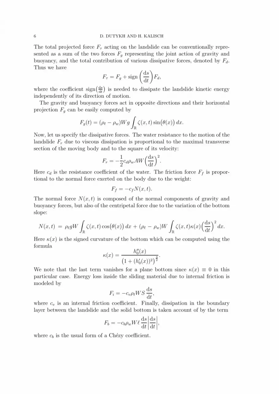
Figure 2. This figure shows velocity and acceleration of the barycenterof the landslide as functions of dimensional time for three different values

of the friction coefficient cf .

Finally, if we sum up the contributions of all the forces described above, weobtain the following second order differential equation:

(γ + cw)Sd2s

dt2= (γ − 1)g

(

I1(t)− cfσ(t)I2(t))

− σ(t)(

cfγI3(t) +1

2cdA)(ds

dt

)2

− cvγSds

dt− cbℓ

ds

dt

∣

∣

∣

∣

ds

dt

∣

∣

∣

∣

, (2.4)

where γ := ρℓρw

> 1 is the ratio of densities, σ(t) := sign(

dsdt

)

and the integrals

I1,2,3(t) are defined by

I1(t) =

∫

R

ζ(x, t) sin(

θ(x))

dx,

I2(t) =

∫

R

ζ(x, t) cos(

θ(x))

dx,

I3(t) =

∫

R

ζ(x, t)κ(x) dx.

Note also that equation (2.4) was simplified by dividing the both sides by the widthW . In order to obtain a well-posed initial value problem, equation (2.4) has to besupplemented with initial conditions for s(0) and s′(0). In the remainder we alwaystake homogeneous initial conditions, and consider the motion driven only by the


0 50 100 150 200−1

0

1

2

t

vc(t

)

Landslide speed

0 50 100 150 200−0.1

−0.05

0

0.05

0.1

t

ac(t

)

Landslide acceleration

Figure 3. This figure shows the velocity and acceleration of thebarycenter of the landslide as a function of dimensional time. The friction

coefficient is cf = tan(3◦). The discontinuities in the acceleration are due

to the coefficient sign(

dsdt

)

in the definition of the friction force.

gravitational acceleration of the landslide. However, different boundary conditionsmight also be reasonable from a modeling point of view.

In order to approximate solutions of equation (2.4), we employ the Bogacki-Shampine third-order Runge-Kutta scheme. The integrals I1,2,3(t) are computedusing the trapezoidal rule, and once the landslide trajectory s = s(t) is found, weuse equation (2.2) to find its motion x = x(t) in the initial Cartesian coordinatesystem. This yields the bottom motion that drives the fluid solver.

3. The Boussinesq model

Once the motion of the landslide is determined, and therefore the time-dependentbathymetry h(x, t) = h0(x) − ζ(x, t) is given, the next step is to consider thecoupling between the bathymetry variations and the evolution of surface waves.The main assumptions on the fluid are that it is inviscid and incompressible, andthat the flow is irrotational. Under these assumptions, the potential-flow freesurface problem governs the motion of the fluid. However, in the present case,the fluid is shallow, and the waves at the surface are of small amplitude whencompared to the depth of the fluid. In that case, the potential-flow problem maybe simplified, and the model used in this paper is a variant of the so-called classicalBoussinesq system derived by Boussinesq [9].


Let us first consider the case of an even bottom, and a constant fluid depthd0. Denote a typical wave amplitude by a, and a typical wavelength by λ. Theparameter α = a

d0then describes the relative amplitude of the waves, and the

parameter β =d20

λ2 measures the ’shallowness’ of the fluid in comparison to thewavelength. In the case when both α and β are small and approximately of thesame order of magnitude, the system

ηt + d0ux + (ηu)x = 0,

ut + gηx + uux −d203uxxt = 0

(3.1)

may be used as an approximate model for the description of the evolution of thesurface waves and the fluid flow in the case of In (3.1), η denotes the deflection ofthe free surface from its rest position, and u denotes the horizontal fluid velocityat a height z = d0(−1 +

√

1/3) in the fluid column if z is measured from the restposition of the free surface. The same equation appears if the velocity is taken tobe the average of the horizontal velocity over the flow depth.

The system (3.1) was first derived by Peregrine in [39], and falls into a generalclass of Boussinesq systems, as shown in the systematic studies [8, 34]. As opposedto the shallow-water approximation, the pressure is not assumed to be hydrostatic,and the horizontal velocity varies with depth. In fact, the horizontal velocity profileis a quadratic function of z [51].

The derivation of (3.1) given in [39] also featured and extension to non-constantbut time-independent bathymetry. However, the present case of a dynamic bottomprofile calls for a system which allows for time-dependent bathymetry, and such asystem was derived in [52]. Given a bottom topography described by z = −h(x, t),the system takes the form

ηt + hux + (ηu)x + ht = 0,

ut + gηx + uux =h2

6uxxt +

1

2h (ht + (hu)x)xt .

(3.2)

In order for this system to be asymptotically valid, we need α ∼ β as before.Moreover, concerning the unsteady bottom profile, we make the assumptions thathx ≤ O(αβ1/2), and ht ≤ O(αβ1/2).

Since this article will also feature a comparison with the shallow-water theory,we mention that the shallow-water system takes the form

ηt + h0ux + (ηu)x = −ht,

ut + gηx + uux = 0(3.3)

in the case of time-dependent bathymetry.In comparison to the shallow-water equations with a time-dependent bottom

topography, the system which is studied here has additional terms in the secondequation of (3.2). The effect of these terms is that dispersion is accounted for.One practical aspect of this modification is that wave breaking can be completely


avoided as long as the amplitude of the waves is small enough. Wave breakingis also possible in evolution systems of Boussinesq type [6], but the amplitudesoccurring in the present problem are far from the breaking limit. One may arguethat the dispersion in (3.2) is too strong in comparison with dispersion in realis-tic water waves. However, the linear dispersion relation of (3.2) with fixed evenbottom is closer to the dispersion relation of the original water-wave problem thanthe KdV equation, or most other types of Boussinesq equations [6].

4. Solitary waves

Before the numerical method for approximating solutions of (3.2) is presented,we digress for a moment, and explain how to find exact solutions of the system(3.1). These exact solutions will later be used to test the implementation of thenumerical procedure.

One exact solution of (3.1) is the traveling wave given by the formula

η(x, t) = −1, u(x, t) = 3 sech

(√3

2ξ

)

, ξ := x− cst.

However, this solution may not be very relevant for the study of surface wavesbecause it represents a constant depression of the surface by −1 which does notappear to be physically possible.

On the other hand, many systems such as (3.1) also have solitary wave solutions,which feature decay of both η and u to zero as x → ∞. Assuming the special form

η(x, t) = η(ξ), u(x, t) = u(ξ), ξ := x− cst,

and substituting this representation into the governing equations (3.1), there ap-pears

−csη′ +(

(d+ η)u)′

= 0,

−csu′ +

1

2(u2)′ + gη′ + cs

d2

3u′′′ = 0.

Integration of the mass conservation equation from −∞ to ξ gives the followingrelation between η and u:

u =csη

d+ η, η =

d · ucs − u

. (4.1)

The momentum balance equation can now be integrated to yield

− cs

(

u− d2

3u′′

)

+1

2u2 + gη = 0. (4.2)

Finally, in order to obtain a closed form equation in terms of the velocity u, wesubstitute the expression (4.1) for η into (4.2). The resulting differential equationcan be written in operator notation as

Lu = N (u),


−10 −5 0 5 10

0

0.05

0.1

0.15

0.2

0.25

0.3

0.35

0.4

0.45

0.5

Free surface elevation

x

η(x

)

Peregrine systemGrimshaw solution

c = 1.05

c = 1.15

c = 1.1

c = 1.2

−10 −5 0 5 10

0

0.05

0.1

0.15

0.2

0.25Depth−averaged horizontal velocity

x

u(x

)

Peregrine systemGrimshaw solution

c = 1.025

c = 1.05

c = 1.1

c = 1.12

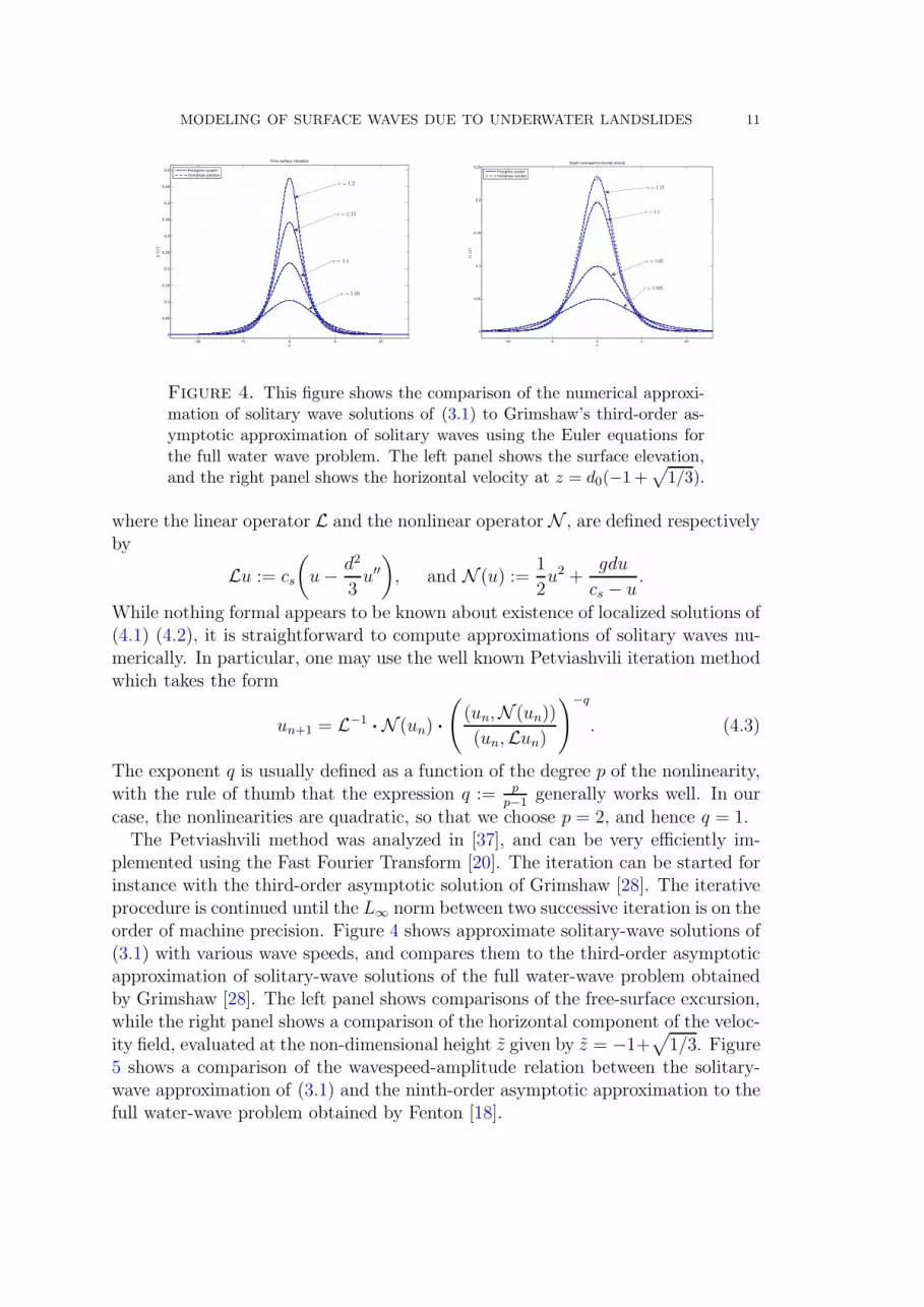
Figure 4. This figure shows the comparison of the numerical approxi-mation of solitary wave solutions of (3.1) to Grimshaw’s third-order as-ymptotic approximation of solitary waves using the Euler equations for

the full water wave problem. The left panel shows the surface elevation,and the right panel shows the horizontal velocity at z = d0(−1 +

√

1/3).

where the linear operator L and the nonlinear operator N , are defined respectivelyby

Lu := cs

(

u− d2

3u′′

)

, and N (u) :=1

2u2 +

gdu

cs − u.

While nothing formal appears to be known about existence of localized solutions of(4.1) (4.2), it is straightforward to compute approximations of solitary waves nu-merically. In particular, one may use the well known Petviashvili iteration methodwhich takes the form

un+1 = L−1·N (un) ·

(

(un,N (un))

(un,Lun)

)−q

. (4.3)

The exponent q is usually defined as a function of the degree p of the nonlinearity,with the rule of thumb that the expression q := p

p−1generally works well. In our

case, the nonlinearities are quadratic, so that we choose p = 2, and hence q = 1.The Petviashvili method was analyzed in [37], and can be very efficiently im-

plemented using the Fast Fourier Transform [20]. The iteration can be started forinstance with the third-order asymptotic solution of Grimshaw [28]. The iterativeprocedure is continued until the L∞ norm between two successive iteration is on theorder of machine precision. Figure 4 shows approximate solitary-wave solutions of(3.1) with various wave speeds, and compares them to the third-order asymptoticapproximation of solitary-wave solutions of the full water-wave problem obtainedby Grimshaw [28]. The left panel shows comparisons of the free-surface excursion,while the right panel shows a comparison of the horizontal component of the veloc-ity field, evaluated at the non-dimensional height z given by z = −1+

√

1/3. Figure5 shows a comparison of the wavespeed-amplitude relation between the solitary-wave approximation of (3.1) and the ninth-order asymptotic approximation to thefull water-wave problem obtained by Fenton [18].


0 0.05 0.1 0.15 0.2 0.25 0.3 0.351

1.02

1.04

1.06

1.08

1.1

1.12

1.14

1.16

Amplitude − Wave speed diagram

a0/d

c s/(gd

)1/2

Fenton solutionClassical Peregrine

Figure 5. This figure shows the amplitude-speed relation of solitarywave solutions of (3.1) and of Fenton’s ninth-order asymptotic approxi-mation of solitary waves using the Euler equations for the full water waveproblem.

5. The numerical scheme

For the numerical discretization, a finite-volume discretization procedure similarto the one used in [3, 4] is employed. Let us take as a unit of length the undisturbeddepth d0 of the fluid above the barycenter of the landslide, and as a unit of time

the ratio√

d0g. Then the Peregrine system (3.2) is rewritten in terms of the total

water depth H as

Ht + [Hu]x = 0, (5.1)

ut +[

12u2 + (H − h)

]

x=

1

2hhxtt +

1

2h(hu)xxt −

1

6h2uxxt, (5.2)

The system (5.1),(5.2) can be formally rewritten in the form

Vt + [F(V) ]x = Sb + M(V), (5.3)

where the density V and the advective flux F(V) are defined by

V ≡(

hu

)

, F(V) ≡(

H u12u2 + (H − h)

)

.

The source term is defined by

Sb ≡(

012hhxtt

)

,

and the dispersive term is defined by

M(V) ≡(

012h(hu)xtt − 1

6h2uxxt

)

.


We begin our presentation by a discretization of the hyperbolic part of the equa-tions which are simply the classical nonlinear shallow-water equations (3.3), andthen discuss the treatment of dispersive terms. The Jacobian of the advective fluxF(V) is easily computed to be

A(V) =∂ F(V)

∂V=

(

u H1 u

)

,

and it is clear that A(V) has the two distinct eigenvalues

λ± = u ± cs, cs ≡√H.

The corresponding right and left eigenvectors are the columns of the matrices

R =

(

H −Hcs cs

)

, L = R−1 =1

2

(

H−1 c−1s

−H−1 c−1s

)

.

We consider a partition of the real line R into cells (or finite volumes) Ci =[xi− 1

2

, xi+ 1

2

] with cell centers xi = 12(xi− 1

2

+ xi+ 1

2

) (i ∈ Z). Let ∆xi denote the

length of the cell Ci. In the sequel we will consider only uniform partitions with∆xi = ∆x, ∀i ∈ Z. We would like to approximate the solution V(x, t) by discretevalues. In order to do so, we introduce the cell average of V on the cell Ci (denotedwith an overbar), i.e.,

Vi(t) ≡(

H i(t) , ui(t))

=1

∆x

∫

Ci

V(x, t) dx.

A simple integration of (5.3) over the cell Ci leads to the exact relation

dV

dt+

1

∆x

[

F(V(xi+ 1

2

, t)) − F(V(xi− 1

2

, t))]

=1

∆x

∫

Ci

Sb(V) dx ≡ Si.

Since the discrete solution is discontinuous at cell interfaces xi+ 1

2

(i ∈ Z), we

replace the flux at the cell faces by the so-called numerical flux function

F(V(xi± 1

2

, t)) ≈ Fi± 1

2

(VLi± 1

2

, VRi± 1

2

),

where VL,R

i± 1

2

denotes the reconstructions of the conservative variables V from left

and right sides of each cell interface (the reconstruction procedure employed in thepresent study will be described below). Consequently, the semi-discrete schemetakes the form

dVi

dt+

1

∆x

[

Fi+ 1

2

− Fi− 1

2

]

= Si. (5.4)

In order to discretize the advective flux F(V), we follow the method of [22, 23]and use the following FVCF scheme

F(V,W) =F(V) + F(W)

2− U(V,W) ·

F(W) − F(V)

2.

The first part of the numerical flux is centered, the second part is the upwindingintroduced through the Jacobian sign-matrix U(V,W) defined by

U(V,W) = sign[

A(12(V +W))

]

, sign(A) = R · diag(s+, s−) · L,


where s± ≡ sign(λ±). After some simple algebraic computations, one can find

U =1

2

(

s+ + s− (H/cs) (s+ − s−)

(cs/H) (s+ − s−) s+ + s−

)

,

the sign-matrix U being evaluated at the average state of left and right values.Finally the source term Sb(x, t) = (0, 1

2hhxtt), which is due to the moving bottom,

is discretized by evaluating the bathymetry function and its derivatives at cellcenters:

1

∆x

∫

Ci

Sb(x, t) dx ≈(

0, 12h(xi, t) hxtt(xi, t)

)

.

Recall that the bathymetry is composed of the static part and of the landslidesubject to a translational motion:

h(x, t) = h0(x)− ζ(x, t) = h0(x)− ζ0(

x− xc(t))

.

The derivative hxtt can be readily obtained from the formula

hxtt(x, t) =d2xc

dt2d2ζ0dx2

(x− xc(t))−(dxc

dt

)2d3ζ0dx3

(x− xc(t)).

5.1. High-order reconstruction. In order to obtain a higher-order scheme inspace, we need to replace the piecewise constant data by a piecewise polynomialrepresentation. This goal is achieved by various so-called reconstruction proceduressuch as MUSCL TVD [33, 48, 49], UNO [31], ENO [30], WENO [53] and manyothers. In one of recent studies on Boussinesq-type equations [17], the UNO2scheme showed a good performance with small dissipation in realistic propagationand run-up simulations. Consequently, we retain this scheme for the discretizationof the advective flux of the Peregrine system (5.1), (5.2).

The main idea of the UNO2 scheme is to construct a non-oscillatory piecewise-parabolic interpolant Q(x) to a piecewise smooth function V(x) (see [31] for moredetails). On each segment containing the face xi+ 1

2

∈ [xi, xi+1], the function

Q(x) = qi+ 1

2

(x) is locally a quadratic polynomial and wherever v(x) is smooth

we have

Q(x) − V(x) = 0 + O(∆x3),dQ

dx(x± 0) − dV

dx= 0 + O(∆x2).

Also, Q(x) should be non-oscillatory in the sense that the number of its localextrema does not exceed that ofV(x). Since qi+ 1

2

(xi) = Vi and qi+ 1

2

(xi+1) = Vi+1,

it can be written in the form

qi+ 1

2

(x) = Vi + di+ 1

2

{V} × x− xi

∆x+ 1

2Di+ 1

2

{V} × (x− xi)(x− xi+1)

∆x2,

where di+ 1

2

{V} ≡ Vi+1− Vi and Di+ 1

2

V is closely related to the second derivative

of the interpolant since Di+ 1

2

{V} = ∆x2 q′′

i+ 1

2

(x). The polynomial qi+ 1

2

(x) is

chosen to be the least oscillatory between two candidates interpolating V(x) at


(xi−1, xi, xi+1) and (xi, xi+1, xi+2). This requirement leads to the following choiceof Di+ 1

2

{V} ≡ minmod(

Di{V},Di+1{V})

with

Di{V} = Vi+1 − 2 Vi + Vi−1, Di+1{V} = Vi+2 − 2 Vi+1 + Vi,

and where minmod(x, y) is the usual minmod function defined as

minmod(x, y) ≡ 12[ sign(x) + sign(y) ]×min(|x|, |y|).

To achieve the second order O(∆x2) accuracy, it is sufficient to consider piece-wise linear reconstructions in each cell. Let L(x) denote this approximately recon-structed function which can be written in this form

L(x) = Vi + Si ·x− xi

∆x, x ∈ [xi− 1

2

, xi+ 1

2

].

In order to L(x) be a non-oscillatory approximation, we use the parabolic interpo-lation Q(x) constructed below to estimate the slopes Si within each cell

Si = ∆x×minmod(dQ

dx(xi − 0),

dQ

dx(xi + 0)

)

.

In other words, the solution is reconstructed on the cells while the solution gradientis estimated on the dual mesh as it is often performed in more modern schemes[3, 4]. A brief summary of the UNO2 reconstruction can be also found in [17].

5.2. Treatment of the dispersive terms. In this section, we explain how wetreat numerically the dispersive terms of the Peregrine system (5.1), (5.2) whichare present only in the momentum conservation equation (5.2). We propose thefollowing approximation for the second component of M(V) of M(V).

Mi(V) =1

2hihi+1(ut)i+1 − 2hi(ut)i + hi−1(ut)i−1

∆x2− 1

6h2i

(ut)i+1 − 2(ut)i + (ut)i−1

∆x2

=hi

2∆x2

(

hi−1 −1

3hi

)

(ut)i−1 +(

1 +2

3∆x2h2i

)

(ut)i +hi

2∆x2

(

hi+1 −1

3hi

)

(ut)i−1.

Note that this spatial discretization is of the second order O(∆x2) so as to beconsistent with the UNO2 advective flux discretization presented above. If wedenote by I the identity matrix, we can now rewrite the semi-discrete scheme inthe form

dH

dt+

1

∆x

[

F(1)+ (V) − F

(1)− (V)

]

= 0,

(I−M) · dudt

+1

∆x

[

F(2)+ (V) − F

(2)− (V)

]

= S(2)b ,

where F(1,2)± (V) are the two components of the advective numerical flux vector F at

the right (+) and left (−) faces correspondingly, and S(2)b denotes the discretization

of the second component of Sb.


5.3. Time stepping. We assume that the linear system of equations is alreadyinverted and we have the following system of ODEs:

Vt = N (V, t), V(0) = V0.

In order to solve numerically the last system of equations, we apply the Bogacki-Shampine method proposed by Przemyslaw Bogacki and Lawrence F. Shampine in1989 [7]. It is a Runge-Kutta scheme of the third order with four stages. It has anembedded second order method which is used to estimate the local error and thus,to adapt the time step size. Moreover, the Bogacki-Shampine method enjoys theFirst Same As Last (FSAL) property so that it needs approximately three functionevaluations per step. This method is also implemented in the ode23 function inMatlab [42]. The one step of the Bogacki-Shampine method is given by:

k1 = N (V(n), tn),

k2 = N (V(n) + 12∆tnk1, tn +

12∆t),

k3 = N (V(n)) + 34∆tnk2, tn +

34∆t),

V(n+1) = V(n) +∆tn(

29k1 +

13k2 +

49k3)

,

k4 = N (V(n+1), tn +∆tn),

V(n+1)2 = V(n) +∆tn

(

424k1 +

14k2 +

13k3 +

18k4)

.

Here V(n) ≈ V(tn), ∆t is the time step and V(n+1)2 is a second order approximation

to the solution V(tn+1), so the difference between V(n+1) and V(n+1)2 gives an

estimation of the local error. The FSAL property consists in the fact that k4 isequal to k1 in the next time step, thus saving one function evaluation.

If the new time step ∆tn+1 is given by ∆tn+1 = ρn∆tn, then according to theH211b digital filter approach [43, 44], the proportionality factor ρn is given by

ρn =( δ

ǫn

)β1( δ

ǫn−1

)β2

ρ−αn−1, (5.5)

where ǫn is a local error estimation at time step tn, and the constants β1, β2 andα are defined by

α =1

4, β1 =

1

4p, β2 =

1

4p.

The parameter p gives the order of the scheme, and p = 3 in our case.

Remark 1. The adaptive strategy (5.5) can be further improved if we smooth the

factor ρn before computing the next time step ∆tn+1:

∆tn+1 = ρn∆tn, ρn = ω(ρn).

The function ω(ρ) is called the time step limiter and should be smooth, monoton-

ically increasing and should satisfy the following conditions:

ω(0) < 1, ω(+∞) > 1, ω(1) = 1, ω′(1) = 1.


10−1

100

10−5

10−4

10−3

10−2

10−1

100

∆x

ε

Convergence rate in L∞ norm

FV scheme, slope = 1.9952nd order

10−1

100

10−5

10−4

10−3

10−2

10−1

100

∆x

ε

Convergence rate in L2 norm

FV scheme, slope = 2.4462nd order

Figure 6. This figure shows the convergence rate of the finite-volumescheme in the L∞-norm (left panel) and the L2-norm (right panel). The

numerical integration of a solitary wave as shown in Figure 4 is comparedto a translated profile. It appears that the second-order convergence is

achieved.

One possible choice was suggested in [44]:

ω(ρ) = 1 + κ arctan(ρ− 1

κ

)

.

In our computations the parameter κ is set to 1.

5.4. Validation. The scheme described in this section is implemented in MAT-LAB, and runs on a workstation. To check whether the implementation is correct,we use the approximate solitary waves of (3.1), computed in the last section. Theseare used as initial data in the fully discrete scheme, and integrated forward in time.The computed solutions are then compared to the same solitary waves, but shiftedforward in space by ct0, where c is the wave speed, and t0 is the final time. Thisprocedure is repeated a number of times with different spatial gridsizes. As a re-sult, it is possible to find the spatial convergence rate of the scheme. As is visiblein Figure 6, the convergence achieved by the practical implementation of the dis-cretization is very close to the theoretical convergence rate. Since the temporaldiscretization is adaptive, we do not present a convergence study in terms of thetimestep.

6. Numerical results and discussion

Let us consider a one-dimensional computational domain I = [a, b] = [0, 220]composed of two regions: the generation region and a sloping beach on the right.More specifically, the static bathymetry function h0(x) is given by a smoothed outprofile generated from the expression

h0(x) =

{

d0 + tan δ · (x− a) + p(x), a ≤ x ≤ m,d0 + tan δ · (m− a)− tan δ · (x−m), x > m,


Symbol Parameter Units Values

g gravitational acceleration m/s2 9.81d0 water depth at x = a m 1.0− 2.0

tan(δ) bottom slope 0.1A landslide amplitude m 0.55l landslide length m 52.4cw added mass coefficient 1.0cd water drag coefficient 1.0cf friction coefficient tan(3◦)γ density ratio water/landslide 1.8cb friction coefficient with bottom 7.63e−4cv viscous friction coefficient 1.27e−3

Table 1. Values of various parameters used in numerical computations.

where the function p(x) is defined as

p(x) = A1sech (k1(x− x1)) + A2sech (k2(x− x2)),

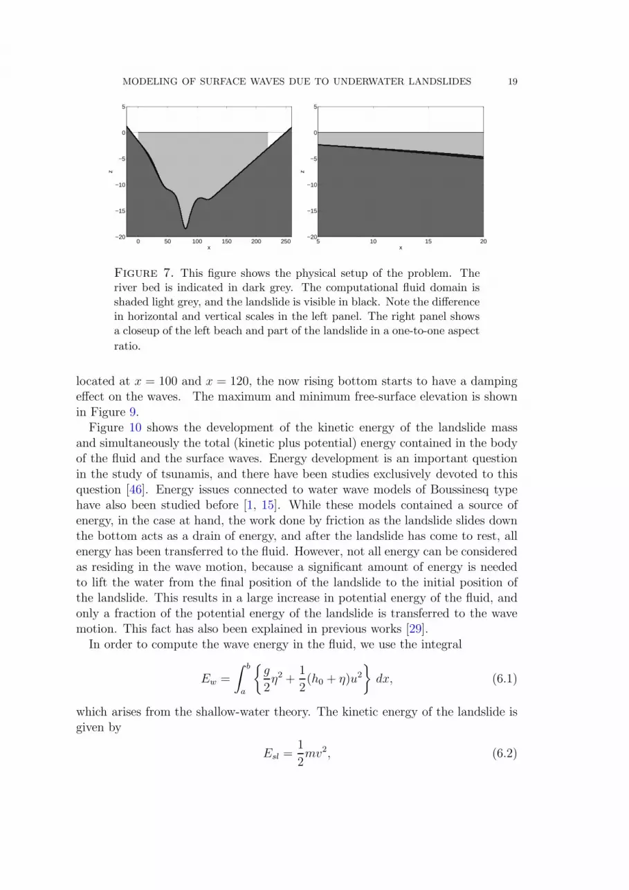
In essence, this function represents a perturbation of the sloping bottom by twounderwater bumps. We made this nontrivial choice in order to illustrate the ad-vantages of our landslide model, which was designed to handle general non-flatbathymmetries. The parameters can be chosen in order to fit a given bathymetry,but the particular values used here are A1 = 4.75, A2 = 8.85, k1 = 0.06, k2 = 0.13,x1 = 45, x2 = 80, and m = 120. The bottom profile for these parameters is de-picted in Figure 7. Of course, in general, if the bottom topography is known, thena numerical bathymetry map could also be used.

We now present some results of the solution of the surface wave problem usingthe model in Section 3, integrated numerically with the method of Section 5. Alandslide is introduced on the left side of the bathymetry, and using the methodof Section 2, its path along the bottom is determined by following the barycen-ter. Simultaneously, the system (3.2) is solved with the time-dependent bottomtopography given from the solution of the landslide problem. The problem is in-tegrated up to a final time T . Figure 8 shows wave records at six virtual wavegauges for both the dispersive system (3.2) and the shallow-water system (3.3).It appears from this figure that the shallow-water system underpredicts the de-velopment of free-surface oscillations. In particular, the wave gauges located atx = 40 and x = 60 show similar waveheights for both the shallow-water, and thedispersive system, but a qualitative divergence, as small oscillations are alreadydeveloping which are not captured by the shallow-water system. Once the waveshave propagated to the wave gauges located at x = 80, the dispersive oscillationshave amplified, so that the waveheight is larger by a factor of 2 to 3 than the wave-height predicted by the shallow-water system. Going further to the wave gauges


x

z

0 50 100 150 200 250−20

−15

−10

−5

0

5

x

z

5 10 15 20−20

−15

−10

−5

0

5

Figure 7. This figure shows the physical setup of the problem. Theriver bed is indicated in dark grey. The computational fluid domain isshaded light grey, and the landslide is visible in black. Note the difference

in horizontal and vertical scales in the left panel. The right panel showsa closeup of the left beach and part of the landslide in a one-to-one aspect

ratio.

located at x = 100 and x = 120, the now rising bottom starts to have a dampingeffect on the waves. The maximum and minimum free-surface elevation is shownin Figure 9.

Figure 10 shows the development of the kinetic energy of the landslide massand simultaneously the total (kinetic plus potential) energy contained in the bodyof the fluid and the surface waves. Energy development is an important questionin the study of tsunamis, and there have been studies exclusively devoted to thisquestion [46]. Energy issues connected to water wave models of Boussinesq typehave also been studied before [1, 15]. While these models contained a source ofenergy, in the case at hand, the work done by friction as the landslide slides downthe bottom acts as a drain of energy, and after the landslide has come to rest, allenergy has been transferred to the fluid. However, not all energy can be consideredas residing in the wave motion, because a significant amount of energy is neededto lift the water from the final position of the landslide to the initial position ofthe landslide. This results in a large increase in potential energy of the fluid, andonly a fraction of the potential energy of the landslide is transferred to the wavemotion. This fact has also been explained in previous works [29].

In order to compute the wave energy in the fluid, we use the integral

Ew =

∫ b

a

{

g

2η2 +

1

2(h0 + η)u2

}

dx, (6.1)

which arises from the shallow-water theory. The kinetic energy of the landslide isgiven by

Esl =1

2mv2, (6.2)


0 50 100 150 200 250−0.4

−0.2

0

0.2

0.4

η(t)/A

x = 40

PeregrineNSWE

0 50 100 150 200 250

−0.4

−0.2

0

0.2

η(t)/A

x = 60.0

PeregrineNSWE

0 50 100 150 200 250

−0.5

0

0.5

η(t)/A

x = 80.0

PeregrineNSWE

0 50 100 150 200 250

−0.2

0

0.2

η(t)/A

x = 100.0

PeregrineNSWE

0 50 100 150 200 250−0.4

−0.2

0

0.2

0.4

t

η(t)/A

x = 120.0

PeregrineNSWE

Figure 8. This figure shows time series of the surface elevation at wavegauges located at x = 40, x = 60, x = 80, x = 100 and x = 120. Thesolid (blue) curve depicts the wave elevation computed with the dispersive

system (3.2), and the dashed curve represents results obtained from theshallow-water system (3.3). All variables are non-dimensional.

with the generalized mass m given by (2.3), and v = dsdt

as defined in Section 2.Figure 10 shows the development of the wave energy and kinetic energy of thelandslide. The upper panel shows the energy according to the shallow-water anddispersive model. The lower panel shows the kinetic energy of the landslide. Wehave also computed the Froude number Fr = v√

gh(xc)during the evolution. Here

v is the x-component of the velocity of the barycenter of the landslide, xc is theposition of the barycenter, and h(xc) is the corresponding local water depth. This


0 50 100 150 200 250

−0.4

−0.2

0

0.2

0.4

0.6

t

η(t)/A

Maximum and minimum free surface elevations

Max. free surface (Peregrine)Min. free surface (Pereregrine)Max. free surface (NSWE)Min. free surface (NSWE)

0 50 100 150 200 250

0

0.05

0.1

t

|u(t)|

Maximum absolute value of the horizontal velocity

PeregrineNSWE

Figure 9. This figure shows the maximum and minimum of the surfaceexcursion, and the horizontal velocity as a function of (non-dimensional)

time.

0 10 20 30 40 50 60 70 80 90 1000

0.5

1

1.5

t

E(t)/(ρgd2 0)

Water wave energy evolution

Total energy (Peregrine)Total energy (NSWE)

0 10 20 30 40 50 60 70 80 90 1000

10

20

30

40

t

K(t)

Landslide kinetic energy evolution

Figure 10. This figure shows the development of the wave energy, andthe kinetic energy of the landslide as a function of (non-dimensional) time.

Note that the kinetic energy of the landslide starts from 0 (all energy ispotential) and also ends at 0 (all energy has been dissipated or transferredto the fluid).


0 50 100 150 200 250 300−1

−0.5

0

0.5

1

t

Ra(t)/A

Run−up on the left beach

PeregrineNSWE

0 50 100 150 200 250 300−1

−0.5

0

0.5

1

t

Rb(t)/A

Run−up on the right beach

PeregrineNSWE

Figure 11. This figure shows the run-up on the left and right beach

using (6.4), computed with the dispersive system (solid curve) and thenonlinear shallow-water system (dashed curve) as a function of (non-dimensional) time.

number was always found to be much less than 1 in all numerical experiments.The maximum value was generally about 0.5. To compute the wave run-up anddraw-down, we use exact representations given by Choi et. al. [10] (a similarformula was also derived in [14]). On the right beach, the undisturbed waterdepth at the edge of the computational domain is h = 3, and the distance fromthe computational domain to the shore line is L = 30. Using the shallow-waterwave speed, the travel time of a wave from the edge of the computational domainto the shore is computed as

T =2L√gh

= 2

√

L

gα. (6.3)

Then the formula for the wave run-up R at the shore reads

R =

∫ t−T

0

t− τ

(t− τ)2 − T 2

dη

dτ(x, τ) dτ (6.4)

with x = 220. At the left beach, the undisturbed water depth is h = 1.642, and thedistance to the beach is L = 11.2814. A similar formula can be then be computedfor x = 0.

Figure 11 shows the run-up on the left and right beaches both in the Boussinesqscaling and in the shallow-water theory. While the agreement is fair on the left


0.5 1 1.5 20.5

0.55

0.6

0.65

d0

max(η)/A

Maximal amplitude

0.5 1 1.5 2−0.65

−0.6

−0.55

−0.5

d0

min(η)/A

Minimal amplitude

0.5 1 1.5 20.35

0.4

0.45

0.5

0.55

0.6

d0

max(R

a)/A

Maximal run−up on the left

0.5 1 1.5 20.65

0.7

0.75

d0

max(R

b)/A

Maximal run−up on the right

Figure 12. This figure shows the maximal and minimal wave ampli-

tude, and the maximum run-up on the left and right beaches as a functionof the initial depth of the center of the landslide d0.

beach, it appears immediately that the Boussinesq theory predicts a wave run-up on the right beach which is much larger (roughly by a factor of two) than thewave run-up according to the shallow-water theory. A possible explanation for thisdivergence is the nature of the numerical solver when applied to the shallow-watersystem. In this case, there is continuous numerical dissipation through the handlingof hyperbolic wave breaking. Since the waves do not break in the Boussinesqscaling, the dissipation is not present, or at least much smaller. The difference canalso read off from the comparison of the wave energy in the Boussinesq and shallow-water system provided in Figure 10. It can be seen there that the wave energyin the shallow-water model starts to diverge from the Boussinesq model at non-dimensional time t = 50. The difference between the two increases continuously,until at the final time, the Boussinesq energy is about 50% larger than the shallow-water energy. Note that significant run-up in Figure 11 does not happen untilnon-dimensional time t = 75, at which time the energy in the Boussinesq systemis already much larger than in the shallow-water system. In Figure 12, we haveplotted the maximum wave amplitude, the minimum wave amplitude, and themaximum wave run-up on the left and right beaches. In comparison to previousstudies, such as [27], where an open domain was used, it appears that in our case,


the maximal amplitude, as well as the run-up have a minimum at d0 between 1and 1.5. In [27], it was found that maximum wave amplitude and run-up (on theleft beach) were strictly decreasing functions of d0. The phenomenon of risingamplitude and run-up may be accredited to resonant effects which are absent onan open domain (such as an ocean beach), but cannot be neglected for tsunamisgenerated by landslides in rivers and lakes.

7. Conclusion

The influence of an underwater landslide on surface waves in a closed basin havebeen studied. The key features of the study have been that the motion of theunderwater landslide have been determined by integrating a second-order ordinarydifferential equation derived from first principles of Newtonian mechanics, and thatthe wave motion has been studied in the Boussinesq scaling which allows for bothnonlinear and dispersive effects. The dynamics of the motion of the bottom havebeen developed following recent work in [32]. The Boussinesq model which hasbeen utilized here allows for a dynamic bathymetry, and was derived in [52]. Thenumerical method used in this paper is an extension of the method put forwardin [3, 4]. The results presented in Section 6 clearly show that dispersion mayhave a strong effect on the run-up and draw-down at the beaches. Of course,this difference could be more or less pronounced depending on the particular caseunder study. For example, the divergence between the shallow-water theory andthe dispersive model is stronger at the right beach than at the left beach. Theresults also show that a finite domain exhibits different behaviour than a half-opendomain (such as used in [27]) with respect to the dependence of the wave run-up onthe initial depth of the landslide. While the run-up is a strictly decreasing functionof the initial depth in an open domain, a closed domain appears to exhibit resonanteffects, which make the dependence more complex.

Acknowledgements

The first author would like to thank the University of Bergen for support and hos-pitality during the preparation of this manuscript. Support from the Agence Na-tionale de la Recherche under project number ANR-08-BLAN-0301-01 (MathOcean)is also gratefully acknowledged.

References

[1] A. Ali and H. Kalisch. Energy balance for undular bores. Comptes Rendus Mecanique,

338:67–70, 2010. 19

[2] J.-P. Bardet, C. E. Synolakis, H. L. Davies, F. Imamura, and E. A. Okal. Land-

slide Tsunamis: Recent Findings and Research Directions. Pure and Applied Geophysics,

160:1793–1809, 2003. 2

[3] T. J. Barth. Aspects of unstructured grids and finite-volume solvers for the Euler and Navier-

Stokes equations. Lecture series - van Karman Institute for Fluid Dynamics, 5:1–140, 1994.

12, 15, 24


[4] T. J. Barth and M. Ohlberger. Encyclopedia of Computational Mechanics, Volume 1, Fun-

damentals, chapter Finite Vol. John Wiley and Sons, Ltd, 2004. 12, 15, 24

[5] G. K. Batchelor. An introduction to fluid dynamics, volume 61 of Cambridge mathematical

library. Cambridge University Press, 2000. 5

[6] M. Bjørkavag and H. Kalisch. Wave breaking in Boussinesq models for undular bores. Physics

Letters A, 375:1570–1578, 2011. 10

[7] P. Bogacki and L. F. Shampine. A 3(2) pair of Runge-Kutta formulas. Applied Mathematics

Letters, 2(4):321–325, 1989. 16

[8] J. L. Bona, M. Chen, and J.-C. Saut. Boussinesq equations and other systems for small-

amplitude long waves in nonlinear dispersive media. I: Derivation and linear theory. Journal

of Nonlinear Science, 12:283–318, 2002. 9

[9] J. Boussinesq. Theorie de l’intumescence liquide appelee onde solitaire ou de translation se

propageant dans un canal rectangulaire. Comptes Rendus de l’Academie des Sciences Ser.

A-B, 72:755–759, 1871. 3, 8

[10] B. H. Choi, V. Kaistrenko, K. O. Kim, B. I. Min, and E. Pelinovsky. Rapid forecasting of

tsunami runup heights from 2-D numerical simulations. Natural Hazards and Earth System

Sciences, 11:707–714, 2011. 22

[11] L. B. Chubarov, G. S. Khakimzyanov, and N. Yu. Shokina. Numerical modelling of surface

water waves arising due to movement of underwater landslide on irregular bottom slope. In

Notes on Numerical Fluid Mechanics and Multidisciplinary Design: Computational Science

and High Performance Computing IV, pages 75–91. Springer-Verlag, Berlin, Heidelberg, vol.

115 edition, 2011. 2

[12] M. Di Risio, G. Bellotti, A. Panizzo, and P. De Girolamo. Three-dimensional experiments

on landslide generated waves at a sloping coast. Coastal Engineering, 56(5-6):659–671, 2009.

4

[13] I. Didenkulova, I. Nikolkina, E. Pelinovsky, and N. Zahibo. Tsunami waves generated by

submarine landslides of variable volume: analytical solutions for a basin of variable depth.

Natural Hazards and Earth System Science, 10:2407–2419, 2010. 2

[14] I. Didenkulova and E. Pelinovsky. Run-up of long waves on a beach: the influence of the

incident wave form. Oceanology, 48(1):1–6, 2008. 22

[15] D. Dutykh and F. Dias. Energy of tsunami waves generated by bottom motion. Proceedings

of the Royal Society A, 465:725–744, 2009. 19

[16] D. Dutykh, T. Katsaounis, and D. Mitsotakis. Dispersive wave runup on non-uniform shores.

In J. et al. Fort, editor, Finite Volumes for Complex Applications VI - Problems & Perspec-

tives, pages 389–397, Prague, 2011. Springer Berlin Heidelberg. 2

[17] D. Dutykh, Th. Katsaounis, and D. Mitsotakis. Finite volume schemes for dispersive wave

propagation and runup. Journal of Computational Physics, 230:3035–3061, 2011. 14, 15

[18] J. Fenton. A ninth-order solution for the solitary wave. Journal of Fluid Mechanics,

53(2):257–271, 1972. 11

[19] E. D. Fernandez-Nieto, F. Bouchut, D. Bresch, M. J. Castro-Diaz, and A. Mangeney. A

new Savage-Hutter type model for submarine avalanches and generated tsunami. Journal of

Computational Physics, 227(16):7720–7754, 2008. 2

[20] M. Frigo and S. G. Johnson. The Design and Implementation of FFTW3. Proceedings of the

IEEE, 93(2):216–231, 2005. 11

[21] H. M. Fritz, W. Kongko, A. Moore, B. McAdoo, J. Goff, C. Harbitz, B. Uslu, N. Kalligeris,

D. Suteja, K. Kalsum, V. V. Titov, A. Gusman, H. Latief, E. Santoso, S. Sujoko, D. Djulka-

rnaen, H. Sunendar, and C. Synolakis. Extreme runup from the 17 July 2006 Java tsunami.

Geophysical Research Letters, 34:L12602, 2007. 2


[22] J.-M. Ghidaglia, A. Kumbaro, and G. Le Coq. Une methode volumes-finis a flux car-

acteristiques pour la resolution numerique des systemes hyperboliques de lois de conser-

vation. Comptes Rendus de l’Academie des Sciences I, 322:981–988, 1996. 13

[23] J.-M. Ghidaglia, A. Kumbaro, and G. Le Coq. On the numerical solution to two fluid models

via cell centered finite volume method. European Journal of Mechanics B / Fluids, 20:841–

867, 2001. 13

[24] S. T. Grilli, F. Dias, P. Guyenne, C. Fochesato, and F. Enet. Progress in fully nonlinear

potential flow modeling of 3D extreme ocean waves. In Q.W. Ma, editor, Advances in Nu-

merical Simulation of Nonlinear Water Waves, pages 75–128. World Scientific Publishing,

2010. 2

[25] S. T. Grilli, P. Guyenne and F. Dias. A fully nonlinear model for three-dimensional overturn-

ing waves over an arbitrary bottom. International Journal of Numerical Methods in Fluids

35:829–867, 2001. 2

[26] S. T. Grilli and P. Watts. Modeling of waves generated by a moving submerged body. Appli-

cations to underwater landslides. Engineering Analysis with boundary elements, 23:645–656,

1999. 2

[27] S. T. Grilli and P. Watts. Tsunami Generation by Submarine Mass Failure. I: Modeling,

Experimental Validation, and Sensitivity Analyses. Journal of Waterway Port Coastal and

Ocean Engineering, 131(6):283, 2005. 2, 3, 23, 24

[28] R. Grimshaw. The solitary wave in water of variable depth. Part 2. Journal of Fluid Me-

chanics, 46:611–622, 1971. 11

[29] C. B. Harbitz, F. Lovholt, G. Pedersen, S. Glimsdal, and D. G. Masson. Mechanisms of

tsunami generation by submarine landslides - a short review. Norwegian Journal of Geology,

86(3):255–264, 2006. 3, 19

[30] A. Harten. ENO schemes with subcell resolution. Journal of Computational Physics, 83:148–

184, 1989. 14

[31] A. Harten and S. Osher. Uniformly high-order accurate nonoscillatory schemes, I. SIAM

Journal of Numerical Analysis, 24:279–309, 1987. 14

[32] G. S. Khakimzyanov and N. Y. Shokina. Numerical modelling of surface water waves arising

due to a movement of the underwater landslide on an irregular bottom. Computational

technologies, 15(1):105–119, 2010. 2, 4, 24

[33] N. E. Kolgan. Finite-difference schemes for computation of three dimensional solutions of

gas dynamics and calculation of a flow over a body under an angle of attack. Uchenye Zapiski

TsaGI [Sci. Notes Central Inst. Aerodyn], 6(2):1–6, 1975. 14

[34] O. Nwogu. Alternative form of Boussinesq equations for nearshore wave propagation. Journal

of Waterway, Port, Coastal and Ocean Engineering, 119:618–638, 1993. 9

[35] E. A. Okal. Normal mode energetics for far-field tsunamis generated by dislocations and

landslides. Pure and Applied Geophysics, 160:2189–2221, 2003. 2

[36] E. A. Okal and C. E. Synolakis. A theoretical comparison of tsunamis from dislocations and

landslides. Pure and Applied Geophysics, 160:2177–2188, 2003. 2

[37] D. E. Pelinovsky and Y. A. Stepanyants. Convergence of Petviashvili’s iteration method for

numerical approximation of stationary solutions of nonlinear wave equations. SIAM Journal

of Numerical Analysis, 42:1110–1127, 2004. 11

[38] E. Pelinovsky and A. Poplavsky. Simplified model of tsunami generation by submarine land-

slides. Physics and Chemistry of the Earth, 21(12):13–17, 1996. 4

[39] D. H. Peregrine. Long waves on a beach. Journal of Fluid Mechanics, 27:815–827, 1967. 9

[40] R. Poncet, C. Campbell, F. Dias, J. Locat, and D. Mosher. A study of the tsunami effects of

two landslides in the St. Lawrence estuary. In D. C. et al. Mosher, editor, Submarine Mass

Movements and Their Consequences, pages 755–764. Springer Verlag, 2010. 2, 3


[41] D. B. Prior and J. M. Coleman. Submarine landslides: geometry and nomenclature.

Zeitschrift fur Geomorphologie, 23:415–426, 1979. 2

[42] L. F. Shampine and M. W. Reichelt. The MATLAB ODE Suite. SIAM Journal on Scientific

Computing, 18:1–22, 1997. 16

[43] G. Soderlind. Digital filters in adaptive time-stepping. ACM Transaction on Mathematical

Software, 29:1–26, 2003. 16

[44] G. Soderlind and L. Wang. Adaptive time-stepping and computational stability. Journal of

Computational and Applied Mathematics, 185(2):225–243, 2006. 16, 17

[45] S. Tadepalli and Synolakis C. E. Model for the leading waves of tsunamis. Physical Review

Letters., 77:2141–2144, 1996. 2

[46] S. Tinti and E. Bortolucci. Energy of Water Waves Induced by Submarine Landslides. Pure

and Applied Geophysics, 157:281–318, 2000. 19

[47] S. Tinti, E. Bortolucci, and C. Chiavettieri. Tsunami Excitation by Submarine Slides in

Shallow-water Approximation. Pure and Applied Geophysics, 158:759–797, 2001. 2

[48] B. van Leer. Towards the ultimate conservative difference scheme V: a second order sequel

to Godunov’ method. Journal of Computational Physics, 32:101–136, 1979. 14

[49] B. van Leer. Upwind and High-Resolution Methods for Compressible Flow: From Donor Cell

to Residual-Distribution Schemes. Communications in Computational Physics, 1:192–206,

2006. 14

[50] P. Watts, F. Imamura, and S. T. Grilli. Comparing model simulations of three benchmark

tsunami generation cases. Science of Tsunami Hazards, 18(2):107–123, 2000. 4

[51] G. B. Whitham. Linear and nonlinear waves. John Wiley & Sons Inc., New York, 1999. 9

[52] T. Y. T. Wu. Generation of upstream advancing solitons by moving disturbances. Journal

of Fluid Mechanics, 184:75–99, 1987. 3, 9, 24

[53] Y. Xing and C.-W. Shu. High order finite difference WENO schemes with the exact conser-

vation property for the shallow water equations. Journal of Computational Physics, 208:206–

227, 2005. 14

LAMA, UMR 5127 CNRS, Universite de Savoie, Campus Scientifique, 73376 Le

Bourget-du-Lac Cedex, France

E-mail address : [email protected]

URL: http://www.lama.univ-savoie.fr/~dutykh/

Department of Mathematics, University of Bergen, Postbox 7800, 5020 Bergen,

Norway

E-mail address : [email protected]

URL: http://folk.uib.no/hka002/

boussinesq modeling of surface waves due to underwater landslides

Documents