calculation of solitary wave shoaling on plane beaches by extended boussinesq equations

Engineering Applications of Computational Fluid Mechanics Vol. 6, No. 1, pp. 25–38 (2012)

Received: 16 Jan. 2011; Revised: 23 Jul. 2011; Accepted: 9 Aug. 2011

25

CALCULATION OF SOLITARY WAVE SHOALING ON PLANE

BEACHES BY EXTENDED BOUSSINESQ EQUATIONS

Parviz Ghadimi *, Mohammad Hadi Jabbari and Arsham Reisinezhad

Department of Marine technology, Amirkabir University of Technology, Teheran, Iran

* E-Mail: [email protected] (Corresponding Author)

ABSTRACT: In this study, shoaling phenomenon is analyzed using Galerkin finite element approach. This

numerical scheme is applied to the extended Boussinesq equations derived by Beji and Nadaoka (1996) for

simulation of shoaling on plane beaches. For spatial discretization, quadratic elements with three-station Lagrange

interpolation polynomials are used for horizontal velocity and the water surface elevation. However, for time

discretization, two different numerical schemes are used. The first method is a combination of semi-implicit schemes

with low-order backward finite difference for time integration and the second method is high-order Adam-

Bashforth-Moulton predictor-corrector strategy. Based on this numerical approach, shoaling phenomenon caused by

propagation of a solitary wave on sloped beaches is modeled and the results are compared with the available results

from the fully nonlinear potential flow model. Considering the fact that the extended Boussinesq equations are

affected by nonlinear effects, a non-dimensional parameter called “Asymmetric Parameter” is introduced. This

parameter expresses the effects of the travelled distance of the solitary wave as well as the relative wave height on

the resulting wave asymmetry. Finally, using this parameter, shoaling coefficient has been computed in an

appropriate range.

Keywords: shoaling coefficient, solitary waves, extended boussinesq equation, finite element approximation,

asymmetric parameter

1. INTRODUCTION

Boussinesq equations have been commonly used

to describe weakly nonlinear and weakly

dispersive properties of wave propagation in

shallow waters. These equations include the low-

order effect of frequency dispersion and

nonlinearity. Nonlinear effect is denoted by the

ratio of wave amplitude to the water depth

(δ=𝜂0/h0) and frequency dispersion is defined by

the square of the ratio of water depth to

wavelength, i.e. μ2= (h0/L0)

2. In Boussinesq

equations, the dependent variables can be

identified in different ways and typical velocity

variables include the surface velocity, the bottom

velocity, the depth-averaged velocity, the velocity

at an arbitrary depth, and the depth-integrated

velocity, as expressed by Madsen and Sorensen

(1992).

Standard Boussinesq equations for variable water

depth derived by peregrine (1967) are based on

the assumptions of δ<< 1 and μ<< 1 and has good

linear accuracy up to 𝑘𝑕 ≈ 0.75 (k is the wave

number). Linearized dispersion property of the

standard Boussinesq equations has been

drastically improved and can even be applied to

relatively deep water, i.e. for the range of 𝑘𝑕 ≤ 3,

in which case, they are known as extended

Boussinesq equations. Extended form of

Boussinesq equations with improved dispersive

properties of the equations have been derived by

Madsen et al. (1991), Nwogu (1993), and Beji

and Nadaoka (1996). Madsen et al. (1991)

introduced some higher-order terms in the

momentum equations which were conventionally

neglected in the process of deriving the

Boussinesq equations. Nwogu (1993) derived an

alternative form of the Boussinesq equations from

the continuity equation and Euler’s equations of

motion. He used the velocity at a certain depth as

a dependent variable. Beji and Nadaoka (1996),

by a simple algebraic manipulation of the

Peregrine’s original equation, designed a

particular form of extended Boussinesq equations.

Ouahsine et al. (2008) also presented an extended

Boussinesq model based on the spectral approach

of the finite element method to improve the

dispersion relationship of the wave propagation in

deeper water.

Until now, there does not appear to be any case

where the dispersion and asymmetry of the

solitary wave propagation over sloped beaches

have been considered or addressed by any type of

Boussinesq equations. For this reason, in the

current study, Beji and Nadaoka (1996)

Boussinesq equations are applied for the

Engineering Applications of Computational Fluid Mechanics Vol. 6, No. 1 (2012)

26

simulation of wave shoaling on slopes where

nonlinearity increases for waves near the breaking

point. However, unlike the fully nonlinear and

dispersive models (Wei et al., 1995; Gobbi et al.,

2000; Madsen et al., 2002; Lynett and Liu, 2004;

Li, 2008; Karambas and Memos, 2009), the

extended Boussinesq equations does not model

the extreme nonlinearity effects near the wave

breaking region, thus determination of a suitable

or reliable range for application of these equations

becomes imperative. Accordingly, in the current

study, using the extended Boussinesq equations,

the propagation of solitary waves over sloped

beaches (gentle (<1:35) and steep (≤1:8) slopes)

are simulated until their breaking points.

Subsequently, by applying different numerical

methods and introducing different wave

geometric parameters, which will be later

identified as asymmetric parameter, an effort will

be made to determine the applicability range of

these equations. As pointed out earlier, due to the

type of depth averaging performed to derive the

Boussinesq equations, these equations are not

capable of modeling wave breaking. Therefore,

much effort has been devoted to develop the

Boussinesq equations. Schäffer et al. (1993)

incorporated a simple description of water wave

breaking in shallow water into the Boussinesq

equations by using the concept of surface roller.

The effect of the roller was included in the

vertical distribution of the horizontal velocity,

which leads to an additional convective

momentum term. The initiation or cessation of

breaking is governed by the maximum surface

slope at each wave front. Kennedy et al. (2000)

used a momentum-conserving eddy viscosity

technique to model the breaking by the

Boussinesq equations. They performed shoaling

and breaking tests involving regular waves. Eddy

viscosity formulation may have some difficulties

in simultaneously providing reliable predictions

of wave heights and horizontal asymmetries in the

inner surf zone. Hirayama and Hara (2003)

presented a wave breaking model that does not

depend on the bottom slope and introduced a

judging function. As part of their model, vertical

water pressure gradient decreases at the wave

breaking point. This model, however, cannot

reproduce the wave breaking on a gentle slope.

Tonelli and Petti (2009) provided coupled

solution of Boussinesq equations and nonlinear

sallow water equations (NSWE) under waves’

physical behavior effects when they move into

shallow water areas and where dispersive terms

become negligible compared to nonlinear terms.

They conducted numerical investigation on

regular wave breaking on a gently sloping beach.

Cienfuegos et al. (2010) developed a new wave-

breaking model for Boussinesq type equations.

They included roller effects in the mass

conservation equation to model the breaking

wave. Their model was also applied to the solitary

wave breaking on a beach.

The above presented methods have also, in recent

years, been applied to other cases to some extent

and among them are the work done by

Orszaghova et al. (2010) and Tonelli and Petti

(2011). In the present numerical study, two

coupled finite element schemes have been utilized

to predict the height of solitary wave propagation

over sloped beaches in a way that the presence of

diffusion terms in the Boussinesq equations is

avoided. Also, in addition to introducing an

asymmetric parameter, the wave geometrical

profile has been used to determine the critical

region of wave breaking.

In recent years, Boussinesq equations have been

solved using finite element schemes by many

researchers; Taylor-Galerkin method by Ambrosi

and Quartapelle (1998), Galerkin technique using

linear elements by Kawahara and Cheng (1994),

Langtangen and Pedersen (1996), Li et al. (1999),

Walkley and Berzins (1999 and 2002), Sørensen

et al. (2004), Zaho et al. (2004) and Ghadimi et al.

(2011), Galerkin technique using high-order

elements by Antunes Do Carmo et al. (1993) and

Langtangen and Pedersen (1998), Petrov-Galerkin

scheme by Woo and Liu (2001) and Avilez-

Valente and Seabra-Santos (2008), and

discontinuous Galerkin method by Engsig-Karup

et al. (2006) are among the most significant works

that can be cited. In this paper, a standard

Galerkin finite element method is applied for

modeling the shoaling phenomena of a solitary

wave.

Similar to the existing numerical methods for

discretization of the spatial terms in Boussinesq

equations, there are several schemes for

discretization of the temporal terms in these

equations. During the developing period of the

Boussinesq equations, various numerical

techniques have been used for time discretizaion

along with spatial discretization. Implementation

of different methods of time discretization have

been done primarily for the purpose of achieving

numerical stability over time as such that the

simulation stays stable for a longer period. Thus,

based on the method of discretization of spatial

terms, the discretization technique of time terms

becomes important, too. Research shows that over

the developing period of Boussinesq equations,

usage of lower order time schemes can cause non-


27

physical dispersion. For instance, Kawahara and

Cheng (1994) used a simple explicit

approximation in time along with their finite

element scheme. Langtangen and Pedersen (1996)

used a staggered time integration scheme which

allowed them to solve each Boussinesq equation

sequentially rather than in a coupled form.

However, in a subsequent paper (Langtangen and

Pederson, 1998) correction terms to increase the

time accuracy were included to eliminate any

non-physical dispersion.

Wei and Kirby (1995), using a finite difference

technique to model the Nwogu equations, showed

that the application of a fourth order Adams-

Bashforth can substantially reduce the error

associated with non-physical dispersion. Since

then, this approach to integration of the

discretized terms of Boussinesq equations over

time took more notice by researchers. Examples

of this can be seen in the works done by

researchers (Li et al., 1999; Bellotti and

Brocchini, 2001; Hsu et al., 2002, Zhao et al.,

2004; Lin and Man, 2007).

In this paper, one dimensional quadratic elements

with three-station Lagrange interpolation

polynomials are used for spatial discretization of

horizontal velocity and the water surface

elevation. However, for time discretization, two

different numerical schemes are used. The first

method is a combination of semi-implicit schemes

with low-order backward finite difference for

time integration while the second method is a

high-order Adam-Bashforth-Moulton predictor-

corrector strategy.

Results of the computations performed by the

developed code are compared against the

numerical findings of Grilli et al. (1989) which is

based on the fully nonlinear potential flow model

(FNPF(. This model has been extensively tested

against the laboratory data for the case of shoaling

and breaking of the solitary waves by Grilli et al.

(1994) that strikingly has close agreement with

the measured data and thus can be considered as a

reliable source for comparison.

Even though using a time integration method can

cause a reducation in wave height during its

propagation, but in this particular case study (i.e.

determination of shoaling coefficient of the

solitary waves propagating over sloped beaches)

in which propagation time is not too large,

combining this scheme with other high order

terms of time has produced interesting results

which are discussed later in the paper.

2. GOVERNING EQUATIONS

Depth averaged Boussinesq equations with

improved dispersive effects are derived by Beji

and Nadaoka (1996) and are as follows

𝜂𝑡 + ∇. 𝑕 + 𝜂 𝒖 = 0 (1)

𝑢𝑡 + 𝑢𝜕𝑢

𝜕𝑥+ 𝑣

𝜕𝑢

𝜕𝑦+ 𝑔

𝜕𝜂

𝜕𝑥

= 1 + 𝛽 𝑕2

3

𝜕2𝑢𝑡

𝜕𝑥2+

𝑕2

3

𝜕2𝑣𝑡

𝜕𝑥𝜕𝑦+ 𝑕

𝜕𝑕

𝜕𝑥

𝜕𝑢𝑡

𝜕𝑥

+𝑕

2

𝜕𝑕

𝜕𝑦

𝜕𝑣𝑡

𝜕𝑥+

𝑕

2

𝜕𝑕

𝜕𝑥

𝜕𝑣𝑡

𝜕𝑦

+ 𝛽𝑔 𝑕2

3

𝜕3𝜂

𝜕𝑥3+

𝑕2

3

𝜕3𝜂

𝜕𝑥𝜕2𝑦+ 𝑕

𝜕𝑕

𝜕𝑥

𝜕2𝜂

𝜕𝑥2

+𝑕

2

𝜕𝑕

𝜕𝑦

𝜕2𝜂

𝜕𝑥𝜕𝑦+

𝑕

2

𝜕𝑕

𝜕𝑥

𝜕2𝜂

𝜕𝑦2

(2a)

𝑣𝑡 + 𝑢𝜕𝑣

𝜕𝑥+ 𝑣

𝜕𝑣

𝜕𝑦+ 𝑔

𝜕𝜂

𝜕𝑦

= 1 + 𝛽 𝑕2

3

𝜕2𝑢𝑡

𝜕𝑥𝜕𝑦+

𝑕2

3

𝜕2𝑣𝑡

𝜕𝑦2+ 𝑕

𝜕𝑕

𝜕𝑦

𝜕𝑣𝑡

𝜕𝑦

+𝑕

2

𝜕𝑕

𝜕𝑥

𝜕𝑢𝑡

𝜕𝑦+

𝑕

2

𝜕𝑕

𝜕𝑦

𝜕𝑢𝑡

𝜕𝑥

+ 𝛽𝑔 𝑕2

3

𝜕2𝜂

𝜕𝑥2𝜕𝑦+

𝑕2

3

𝜕3𝜂

𝜕𝑦3+ 𝑕

𝜕𝑕

𝜕𝑦

𝜕2𝜂

𝜕𝑦2

+𝑕

2

𝜕𝑕

𝜕𝑥

𝜕2𝜂

𝜕𝑥𝜕𝑦+

𝑕

2

𝜕𝑕

𝜕𝑦

𝜕2𝜂

𝜕𝑥2

(2b)

In these equations, u(u,v) is the two-dimensional

depth averaged velocity vector, η is the water

surface elevation, h(x,y) is the water depth as

measured from the still water level, and g is the

gravitational acceleration. The subscript, t,

denotes partial differentiation with respect to

time.

The dispersion relation for these equations after

linearization for uniform water depth is

𝑐2 =ω2

𝑘2=

𝑔𝑕(1 + β𝑘2𝑕2 3)

1 + (1 + β)𝑘2𝑕2 3 (3)

where c is the wave celerity; ω is the wave

circular frequency and k is the wave number. β is

equal to 1/5 and can be determined by best

matching Eq. (3) with the second order Padé

approximant of the full linear dispersion relation

𝜔2/𝑔𝑘 = 𝑡𝑎𝑛𝑕 𝑘𝑕.

3. NUMERICAL MODEL

3.1 Finite element method

Governing equations (1) and (2) are solved by a

numerical finite element method as follows:


28

Two numerical methods are used to discretize the

equations. In the first method (Method A), spatial

derivatives are discretized by Galerkin finite

element approximation while semi implicit

method is used to discretize the derivatives in

time. In the second method (Method B), spatial

derivatives are discretized in the same way as in

(Method A), but explicit Adams–Bashforth–

Moulton (ABM) method with predictor–corrector

scheme similar to that used by Wei and Kirby

(1995) is applied to discretize derivatives in time.

These two methods which have different

accuracies are applied to discretize the one-

dimensional simplified form of Eqs. (1) and (2),

as outlined below. The one-dimensional form of

equations (1) and (2) is as follows:

𝜂𝑡 +𝜕

𝜕𝑥 𝐻𝑢 = 0 (4)

𝑢𝑡 + 𝑢𝜕𝑢

𝜕𝑥+ 𝑔

𝜕𝜂

𝜕𝑥

= 1 + 𝛽 𝑕 𝑕

3

𝜕2𝑢𝑡

𝜕𝑥2+

𝜕𝑕

𝜕𝑥

𝜕𝑢𝑡

𝜕𝑥

+ 𝛽𝑔𝑕[𝑕

3

𝜕3𝜂

𝜕𝑥3+

𝜕𝑕

𝜕𝑥

𝜕2𝜂

𝜕𝑥2]

(5)

where H = η+ h.

By subdividing computational domain Ω into N

elements, N+1nodes are generated. The

corresponding dependent variables at each point

are approximated within the elements as follows:

𝑓 ≈ 𝑁𝑖𝑓𝑖

𝑛𝑑

𝑖=1

(6)

where 𝑓𝑖 is the value of any dependent variable at

the nodal point(𝑢, 𝜂), nd is the number of nodes

and 𝑁𝑖 is the interpolation function. Due to the

presence of third-spatial derivatives in Eq. (5),

three-station Lagrange interpolation polynomials

are used for 𝑁𝑖 and subsequently integrated.

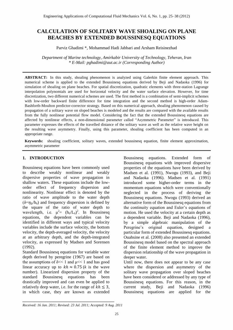
When spatial domain is uniformly discretized

with N linear finite elements, N-1 quadratic

overlapping elements are generated, as shown in

Fig.1. Computational domain of each overlapping

element is denoted by 𝛺𝑒 .

Galerkin method is applied to Eqs. (4) and (5) and

by substituting the depending variables from Eq.

(6), the element matrix equation is found to be:

𝑀𝑘𝑖 𝜂 𝑖

= −𝑄𝑘𝑖𝑗 𝐻 𝑖 𝑢 𝑗 − 𝑄𝑘𝑖𝑗 𝑢 𝑖 𝐻 𝑗 (7)

Fig. 1 1-D system of overlapped elements for

numerical calculation.

𝑀𝑘𝑖 𝑢 𝑖 + 𝑄𝑘𝑖𝑗 𝑢 𝑖 𝑢 𝑗 + 𝑔𝑇𝑘𝑖 𝜂 𝑖

= 1 + 𝛽 𝑕 𝑕

3𝐸𝑘𝑖 +

𝜕𝑕

𝜕𝑥𝑇𝑘𝑖 𝑢 𝑖

+ 𝛽𝑔𝑕 𝑕

3 𝑆𝑘𝑖 − 𝑁𝑘

𝜕2𝑁𝑖

𝜕𝑥2

𝛤𝑒

𝑛𝑥𝑑𝑠

+𝜕𝑕

𝜕𝑥𝐸𝑘𝑖 𝜂 𝑖

(8)

where

𝑀𝑘𝑖 = 𝑁𝑘𝑁𝑖𝑑𝛺

𝛺

𝑘, 𝑖 = 1, 2, 3

(9a)

𝑄𝑘𝑖𝑗 = 𝑁𝑘𝑁𝑖

𝜕𝑁𝑗

𝜕𝑥𝛺

𝑑𝛺

𝑘, 𝑖 = 1, 2, 3

(9b)

𝑇𝑘𝑖 = 𝑁𝑘

𝜕𝑁𝑖

𝜕𝑥𝛺

𝑑𝛺

𝑘, 𝑖 = 1, 2, 3

(9c)

𝐸𝑘𝑖 = 𝑁𝑘

𝜕2𝑁𝑖

𝜕𝑥2

𝛺

𝑑𝛺

𝑘, 𝑖 = 1, 2, 3

(9d)

𝑆𝑘𝑖 = 𝜕𝑁𝑘

𝜕𝑥

𝜕2𝑁𝑖

𝜕𝑥2

𝛺

𝑑𝛺

𝑘, 𝑖 = 1, 2, 3

(9e)


29

3.2 Time integration methods

The time derivatives are discretized using two

different schemes which are explained below:

a) Semi-implicit method: The discretized form of

the nodal values are written as

𝑓 𝑖 = 𝜃 𝑓 𝑖𝑛𝑡 + (1 − 𝜃) 𝑓 𝑖

𝑛𝑡+1 or

𝑓∗ 𝑖 𝑓 𝑗= 𝑓∗ 𝑖

𝑛𝑡 (𝜃 𝑓 𝑗𝑛𝑡 + 1 − 𝜃 𝑓 𝑗

𝑛𝑡+1) (10)

where θ is called the “relaxation coefficient”

ranging from 0 to 1 while 𝑓∗ and 𝑓 are the

dependent nodal variables.

The first terms of equations (7) and (8) are

discretized by backward finite difference as

𝑓𝑡 𝑖 =( 𝑓 𝑖

𝑛𝑡 +1− 𝑓 𝑖𝑛𝑡 )

∆𝑡+ О(∆𝑡) (11)

Upon generation of element matrices and

assemblage of them, global matrix is formed and

solved by a modified SOR solver.

b) Predictor-corrector method: The assembled

global equations corresponding to Eqs. (7) or

(8) can be written in matrix form as

𝑀 𝑓 = 𝑬 (12)

where M is the coefficient matrix and E is a

vector calculated from the known values of

𝜂 𝑜𝑟 𝑢. 𝑓(𝜂, 𝑢) is a vector depending on 𝜂 and

𝑢 variables.

In order for Eq. (8) to become analogous with Eq.

(12), Eq. (8) has been transformed to the

following two equations:

𝑀𝑘𝑖 𝑢 𝑖 = −𝑄𝑘𝑖𝑗 𝑢 𝑖 𝑢 𝑗 − 𝑔𝑇𝑘𝑖 𝜂 𝑖

+ 𝛽𝑔𝑕 𝑕

3 𝑆𝑘𝑖 − 𝑁𝑘

𝜕2𝑁𝑖

𝜕𝑥2

𝛤𝑒

𝑛𝑥𝑑𝑠

+𝜕𝑕

𝜕𝑥𝐸𝑘𝑖 𝜂 𝑖

(13)

𝑀𝑘𝑖 𝑢 𝑖

= 1 + 𝛽 𝑕 𝑕

3 𝐸𝑘𝑖 +

𝜕𝑕

𝜕𝑥 𝑇𝑘𝑖 𝑢 𝑖

+ 𝑀𝑘𝑖 𝑢 𝑖

(14)

If initial conditions are specified, i.e. if the values

of η and u at the time levels of 𝑛 − 2, 𝑛 − 1, and

𝑛 are available, then the solution at the

subsequent time level 𝑛 + 1 can be obtained by

virtue of the following procedure:

1) Evaluation of the right-hand sides of

equations (7) and (13) at time level 𝑛, 𝑛 −1, 𝑛 − 2;

2) Time Integration of equations (7) and (13) by

means of the predictor stage of the ABM

scheme:

𝑀 𝑓 𝑛+1

= 𝑀 𝑓 𝑛

+∆𝑡

12 23 𝐸 𝑛 − 16 𝐸 𝑛−1 + 5 𝐸 𝑛−2

+ 𝑂(∆𝑡3)

(15)

3) Evaluation of 𝑢 from 𝑢 ;

4) Evaluation of right-hand sides of Eqs. (7) and

(13) at time level 𝑛 + 1;

5) Time Integration of equations (7) and (13) by

means of the corrector stage of the ABM

scheme:

𝑀 𝑓 𝑛+1

= 𝑀 𝑓 𝑛

+∆𝑡

24 9 𝐸 𝑛+1 + 19 𝐸 𝑛 − 5 𝐸 𝑛−1

+ 5 𝐸 𝑛−2 + 𝑂(∆𝑡3)

(16)

6) Evaluation of 𝑢 from 𝑢 ;

Steps 4 through 6 are repeated until convergence

is reached, as suggested by Bellotti and Brocchini

(2001).

4. APPLICATION AND RESULTS

4.1 Shoaling of solitary waves on plane

beaches

In this case study, the suggested model is applied

to the shoaling of solitary waves on different

slopes in the hope of offering a new method for

determining the shoaling coefficient of solitary

waves over sloped beaches. The methods of

generating solitary wave are different based on

the type of governing equations involved (Hafsia

et al., 2009). However, the best method for

solving the Boussinesq equations seems to be the

use of the initial water profile which is found

from the exact solution of the weakened type of

the governing equation (Peregrine, 1967).

Accordingly, two solitary waves with different

initial heights, i.e. 𝛿 =𝜂0

𝑕0, propagating over four

different slopes, i.e. S, ranging from gentle

(1:100) to steep (1:8) are considered.


30

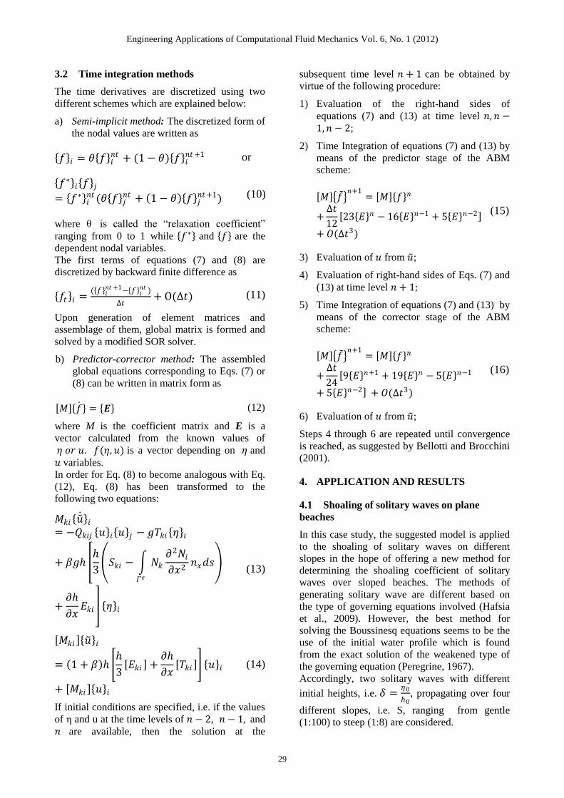
Fig. 2 Schematic of computational domain.

Subsequently, in order to validate the findings,

the obtained results are compared with the

available results of fully nonlinear potential flow

model (FNPF) by Grilli et al. (1994).

The computational domain is illustrated in Fig.2

where 𝑕0, being the constant depth, is considered

to be 0.44 𝑚 in the current study as in the work

denote classical dimensionless variables of long

wave theory; 𝑥′ =𝑥

𝑕0, 𝑡′ = 𝑡/ 𝑕0 𝑔 . To make

the comparison easier, results of computations

were presented at 𝑡′ = 0 at which time the wave

crest is located at 𝑥′ = 0 where the slope starts.

Wave profiles by the present model have been

obtained by two methods, i.e. the semi-implicit

low-order scheme (Method A) and the predictor-

corrector high-order scheme (Method B). Results

of the mentioned schemes are compared with the

available results of FNPF method in Fig.3.

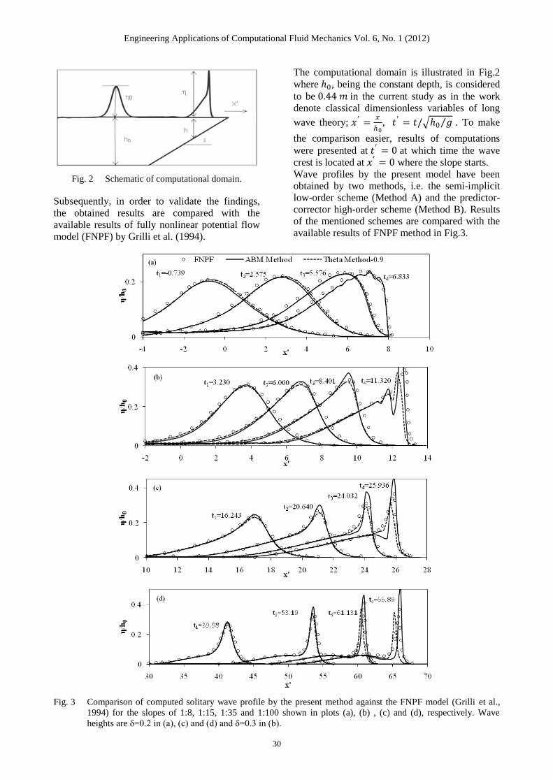
Fig. 3 Comparison of computed solitary wave profile by the present method against the FNPF model (Grilli et al.,

1994) for the slopes of 1:8, 1:15, 1:35 and 1:100 shown in plots (a), (b) , (c) and (d), respectively. Wave

heights are δ=0.2 in (a), (c) and (d) and δ=0.3 in (b).


31

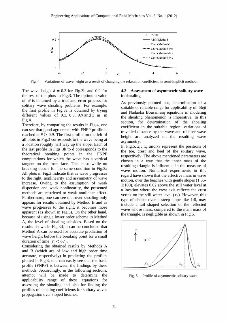
Fig. 4 Variations of wave height as a result of changing the relaxation coefficient in semi-implicit method.

The wave height 𝛿 = 0.3 for Fig.3b and 0.2 for

the rest of the plots in Fig.3. The optimum value

of 𝜃 is obtained by a trial and error process for

solitary wave shoaling problems. For example,

the first profile in Fig.3a is obtained by trying

different values of 0.1, 0.5, 0.9 and 1 as in

Fig.4.

Therefore, by comparing the results in Fig.4, one

can see that good agreement with FNFP profile is

reached at 𝜃 ≥ 0.9. The first profile on the left of

all plots in Fig.3 corresponds to the wave being at

a location roughly half way up the slope. Each of

the last profile in Figs 3b to d corresponds to the

theoretical breaking points in the FNPF

computations for which the wave has a vertical

tangent on the front face. This is so while no

breaking occurs for the same condition in Fig.3a

All plots in Fig.3 indicate that as wave progresses

to the right, nonlinearity and asymmetry of wave

increase. Owing to the assumption of weak

dispersion and weak nonlinearity, the presented

methods are restricted to weak nonlinear effect.

Furthermore, one can see that over shoaling only

appears for results obtained by Method B and as

wave progresses to the right, it becomes more

apparent (as shown in Fig.3). On the other hand,

because of using a lower order scheme in Method

A, the level of shoaling subsides. Based on the

results shown in Fig.3d, it can be concluded that

Method A can be used for accurate prediction of

wave height before the breaking point for a small

duration of time (𝑡 , < 67).

Considering the obtained results by Methods A

and B (which are of low and high order time

accurate, respectively) in predicting the profiles

plotted in Fig.3, one can easily see that the basis

profile (FNPF) is between the findings by these

methods. Accordingly, in the following sections,

attempt will be made to determine the

applicability range of these equations for

assessing the shoaling and also for finding the

profiles of shoaling coefficients for solitary waves

propagation over sloped beaches.

4.2 Assessment of asymmetric solitary wave

in shoaling

As previously pointed out, determination of a

suitable or reliable range for applicability of Beji

and Nadaoka Boussinesq equations in modeling

the shoaling phenomenon is imperative. In this

section, for determination of the shoaling

coefficient in the suitable region, variations of

travelled distance by the wave and relative wave

height are analyzed on the resulting wave

asymmetry.

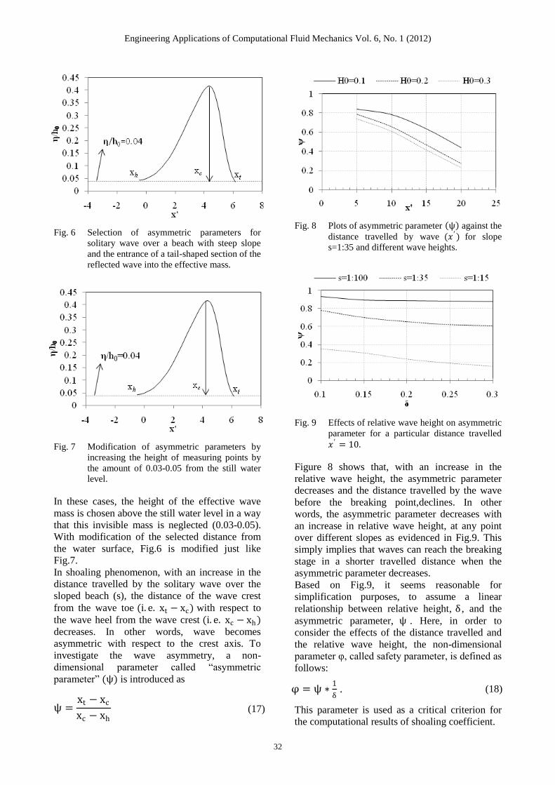
In Fig.5, 𝑥𝑡 , 𝑥𝑐 and 𝑥𝑕 represent the positions of

the toe, crest and heel of the solitary wave,

respectively. The above mentioned parameters are

chosen in a way that the inner mass of the

resulting triangle is influential in the measure of

wave motion. Numerical experiments in this

regard have shown that the effective mass in wave

motion, over the beaches with gentle slopes (1:35-

1:100), elevates 0.02 above the still water level at

a location where the crest axis reflects the crest

vertex on the still water level (𝑥𝑐). However, this

type of choice over a steep slope like 1:8, may

include a tail shaped selection of the reflected

wave whose mass, compared to the main mass of

the triangle, is negligible as shown in Fig.6.

Fig. 5 Profile of asymmetric solitary wave.


32

Fig. 6 Selection of asymmetric parameters for

solitary wave over a beach with steep slope

and the entrance of a tail-shaped section of the

reflected wave into the effective mass.

Fig. 7 Modification of asymmetric parameters by

increasing the height of measuring points by

the amount of 0.03-0.05 from the still water

level.

In these cases, the height of the effective wave

mass is chosen above the still water level in a way

that this invisible mass is neglected (0.03-0.05).

With modification of the selected distance from

the water surface, Fig.6 is modified just like

Fig.7.

In shoaling phenomenon, with an increase in the

distance travelled by the solitary wave over the

sloped beach (s), the distance of the wave crest

from the wave toe (i. e. xt − xc) with respect to

the wave heel from the wave crest (i. e. xc − xh )

decreases. In other words, wave becomes

asymmetric with respect to the crest axis. To

investigate the wave asymmetry, a non-

dimensional parameter called “asymmetric

parameter” (ψ) is introduced as

ψ =xt − xc

xc − xh (17)

Fig. 8 Plots of asymmetric parameter ψ against the

distance travelled by wave (𝑥 ′) for slope

s=1:35 and different wave heights.

Fig. 9 Effects of relative wave height on asymmetric

parameter for a particular distance travelled

𝑥 ′ = 10.

Figure 8 shows that, with an increase in the

relative wave height, the asymmetric parameter

decreases and the distance travelled by the wave

before the breaking point,declines. In other

words, the asymmetric parameter decreases with

an increase in relative wave height, at any point

over different slopes as evidenced in Fig.9. This

simply implies that waves can reach the breaking

stage in a shorter travelled distance when the

asymmetric parameter decreases.

Based on Fig.9, it seems reasonable for

simplification purposes, to assume a linear

relationship between relative height, δ , and the

asymmetric parameter, ψ . Here, in order to

consider the effects of the distance travelled and

the relative wave height, the non-dimensional

parameter φ, called safety parameter, is defined as

follows:

φ = ψ ∗1

δ . (18)

This parameter is used as a critical criterion for

the computational results of shoaling coefficient.


33

4.3 Measurement of the safety parameter

In the proposed modeling of the solitary wave

propagation over sloped beaches, the safety

parameter is measured in two different ways: (1)

using the temporal profile and (2) using the

spatial profile. These two methods are different

from the standpoint of computational accuracy

which will be explained below.

4.3.1 Determination of safety parameter using

temporal profile

In this method, successive gauges are

longitudinally placed in the numerical channel in

the direction of wave propagation over the sloped

beaches. These gauges monitor the water surface

profile from the beginning to the end of the

computational time. These findings are stored in

separate files. These data show the wave motion

from the time of entry to the gauge and complete

exit in terms of the time steps. In this method,

parameters associated with the heel 𝑥𝑕 , toe 𝑥𝑡 ,

and crest xc of the wave for determining the

asymmetric parameter corresponding to their

values (heel, toe, and crest), are placed on the

time axis. This is due to the fact that because of

the linear assumption of the wave velocity, the

location of wave is proportional to time.

4.3.2 Determination of safety parameter using

the spatial profile

In this method, different snap shots (like

photographs) are taken from the water surface

profile at different times of wave propagation

over the sloped beaches. Therefore, a profile of

water surface at different times is obtained which

is placed on the spatial coordinate. It is clear that

the coordinate of each wave corresponding to the

location of the wave crest is situated on the spatial

coordinate.

Each of the proposed methods for determining the

safety parameter has its own strength and

weakness which depends on the length of

computational time and the type of the slope used

in the numerical modeling of the wave

propagation. Data which are obtained from the

temporal profile, because of the small time step

during a time interval, are more numerous and

thus better accuracy is obtained by the data

processing in this case. In comparison, accuracy

of data in the case of using a spatial profile is less

because of the increase in the consumed time for

complete processing of wave propagation over the

sloped beach, the reduction of the size of

elements as much as the time steps is not

economically feasible. Therefore, there are data

limitations in using the spatial profile and

interpolation may become necessary.

On the other hand, using the temporal profile for

beaches with steep slopes is not possible because

the propagated wave would not have sufficient

time for complete passing over the gauges placed

on the sloped beach. In this case, data are

incomplete and thus not usable for determining

the safety factor. Overall, the temporal profile is

recommended to be used for processing data over

the beaches with gentle and mild slopes while the

spatial profile is suggested for beaches with steep

slopes.

For calculating the safety parameter associated

with each profile, a table similar to Tables 1 and 2

must be established. In constructing these tables,

if a temporal profile is used, the wave height is

non-dimensionalized. However, if a spatial profile

is utilized, then the wave height as well as spatial

coordinate are non-dimensionalized.

4.4 Determination of safety parameter for

wave profiles

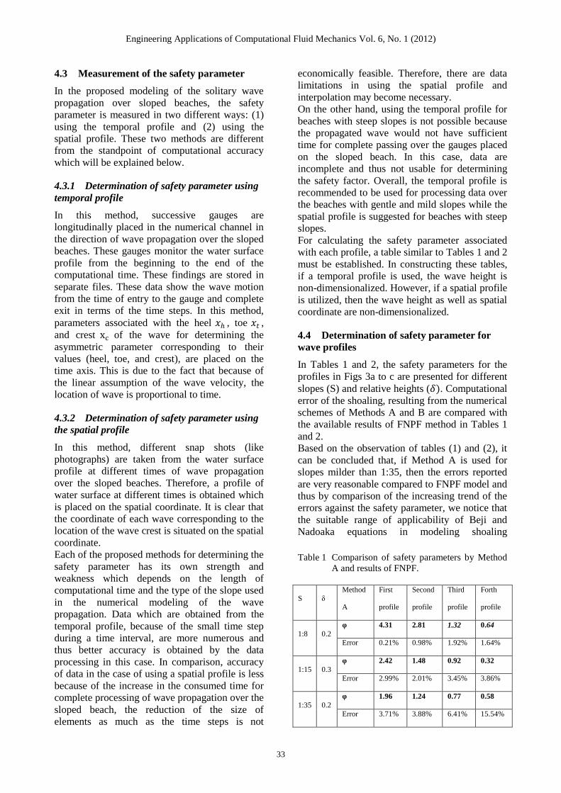
In Tables 1 and 2, the safety parameters for the

profiles in Figs 3a to c are presented for different

slopes (S) and relative heights (𝛿). Computational

error of the shoaling, resulting from the numerical

schemes of Methods A and B are compared with

the available results of FNPF method in Tables 1

and 2.

Based on the observation of tables (1) and (2), it

can be concluded that, if Method A is used for

slopes milder than 1:35, then the errors reported

are very reasonable compared to FNPF model and

thus by comparison of the increasing trend of the

errors against the safety parameter, we notice that

the suitable range of applicability of Beji and

Nadoaka equations in modeling shoaling

Table 1 Comparison of safety parameters by Method

A and results of FNPF.

S δ

Method

A

First

profile

Second

profile

Third

profile

Forth

profile

1:8 0.2

φ 4.31 2.81 1.32 0.64

Error 0.21% 0.98% 1.92% 1.64%

1:15 0.3

φ 2.42 1.48 0.92 0.32

Error 2.99% 2.01% 3.45% 3.86%

1:35 0.2

φ 1.96 1.24 0.77 0.58

Error 3.71% 3.88% 6.41% 15.54%


34

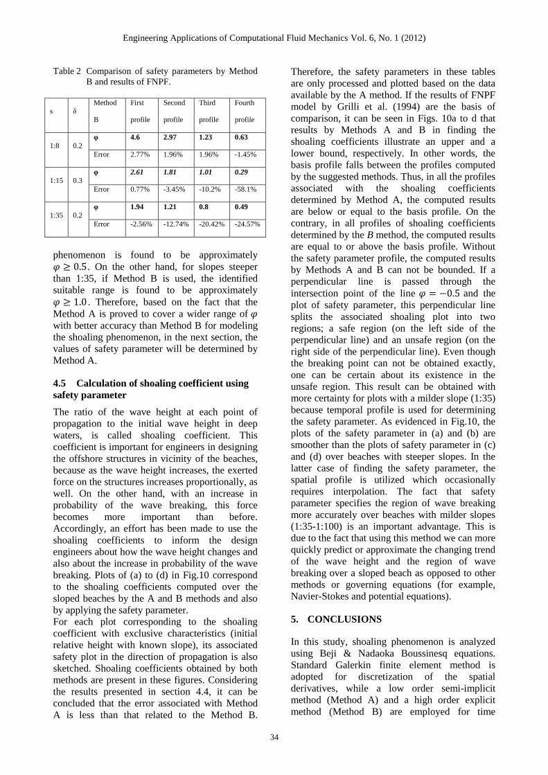
Table 2 Comparison of safety parameters by Method

B and results of FNPF.

s δ Method

B

First

profile

Second

profile

Third

profile

Fourth

profile

1:8 0.2

φ 4.6 2.97 1.23 0.63

Error 2.77% 1.96% 1.96% -1.45%

1:15 0.3

φ 2.61 1.81 1.01 0.29

Error 0.77% -3.45% -10.2% -58.1%

1:35 0.2

φ 1.94 1.21 0.8 0.49

Error -2.56% -12.74% -20.42% -24.57%

phenomenon is found to be approximately

𝜑 ≥ 0.5. On the other hand, for slopes steeper

than 1:35, if Method B is used, the identified

suitable range is found to be approximately

𝜑 ≥ 1.0 . Therefore, based on the fact that the

Method A is proved to cover a wider range of 𝜑

with better accuracy than Method B for modeling

the shoaling phenomenon, in the next section, the

values of safety parameter will be determined by

Method A.

4.5 Calculation of shoaling coefficient using

safety parameter

The ratio of the wave height at each point of

propagation to the initial wave height in deep

waters, is called shoaling coefficient. This

coefficient is important for engineers in designing

the offshore structures in vicinity of the beaches,

because as the wave height increases, the exerted

force on the structures increases proportionally, as

well. On the other hand, with an increase in

probability of the wave breaking, this force

becomes more important than before.

Accordingly, an effort has been made to use the

shoaling coefficients to inform the design

engineers about how the wave height changes and

also about the increase in probability of the wave

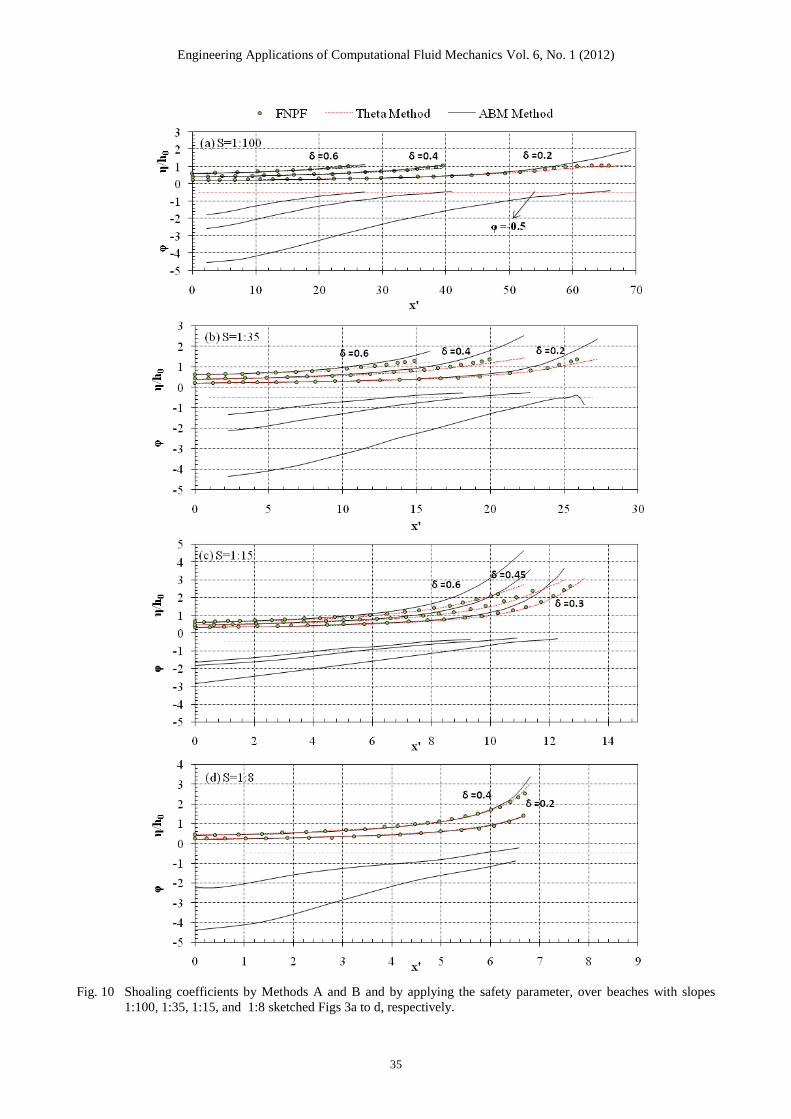
breaking. Plots of (a) to (d) in Fig.10 correspond

to the shoaling coefficients computed over the

sloped beaches by the A and B methods and also

by applying the safety parameter.

For each plot corresponding to the shoaling

coefficient with exclusive characteristics (initial

relative height with known slope), its associated

safety plot in the direction of propagation is also

sketched. Shoaling coefficients obtained by both

methods are present in these figures. Considering

the results presented in section 4.4, it can be

concluded that the error associated with Method

A is less than that related to the Method B.

Therefore, the safety parameters in these tables

are only processed and plotted based on the data

available by the A method. If the results of FNPF

model by Grilli et al. (1994) are the basis of

comparison, it can be seen in Figs. 10a to d that

results by Methods A and B in finding the

shoaling coefficients illustrate an upper and a

lower bound, respectively. In other words, the

basis profile falls between the profiles computed

by the suggested methods. Thus, in all the profiles

associated with the shoaling coefficients

determined by Method A, the computed results

are below or equal to the basis profile. On the

contrary, in all profiles of shoaling coefficients

determined by the B method, the computed results

are equal to or above the basis profile. Without

the safety parameter profile, the computed results

by Methods A and B can not be bounded. If a

perpendicular line is passed through the

intersection point of the line 𝜑 = −0.5 and the

plot of safety parameter, this perpendicular line

splits the associated shoaling plot into two

regions; a safe region (on the left side of the

perpendicular line) and an unsafe region (on the

right side of the perpendicular line). Even though

the breaking point can not be obtained exactly,

one can be certain about its existence in the

unsafe region. This result can be obtained with

more certainty for plots with a milder slope (1:35)

because temporal profile is used for determining

the safety parameter. As evidenced in Fig.10, the

plots of the safety parameter in (a) and (b) are

smoother than the plots of safety parameter in (c)

and (d) over beaches with steeper slopes. In the

latter case of finding the safety parameter, the

spatial profile is utilized which occasionally

requires interpolation. The fact that safety

parameter specifies the region of wave breaking

more accurately over beaches with milder slopes

(1:35-1:100) is an important advantage. This is

due to the fact that using this method we can more

quickly predict or approximate the changing trend

of the wave height and the region of wave

breaking over a sloped beach as opposed to other

methods or governing equations (for example,

Navier-Stokes and potential equations).

5. CONCLUSIONS

In this study, shoaling phenomenon is analyzed

using Beji & Nadaoka Boussinesq equations.

Standard Galerkin finite element method is

adopted for discretization of the spatial

derivatives, while a low order semi-implicit

method (Method A) and a high order explicit

method (Method B) are employed for time


35

Fig. 10 Shoaling coefficients by Methods A and B and by applying the safety parameter, over beaches with slopes

1:100, 1:35, 1:15, and 1:8 sketched Figs 3a to d, respectively.


36

integration. By comparison of the obtained results

from modeling the free surface profiles over the

sloped beach with those of FNPF model, it is

clear that the FNPF results fall between the

profiles produced Methods A and B, albeit the

result of Method A is closer to the FNPF profile.

It is further noted that plots of shoaling

coefficients by FNPF model are bounded below

by the result of Method A and above by the result

of Method B. In order to determine the upper and

lower bounds of this range, the variation of wave

geometry in propagation over the sloped beach

was studied. This study showed that the wave

geometry during the propagation over the sloped

beach becomes asymmetric in a way that the

distance of the wave crest from the wave toe with

respect to the distance of the wave heel from the

wave crest would reduce. This reduction causes

instability in the wave and ultimately brings about

wave breaking. The ratio of the mentioned

distances was initially called asymmetric

parameter. However, since waves with higher

relative height break earlier, this ratio was

redefined as safety parameter which is inversely

proportional to the relative height of the wave.

Furthermore, shoaling coefficients over sloped

beaches were computed using the Methods A and

B. Shoaling coefficients along with their

associated safety parameters were plotted. The

intersection point of the plot of safety parameter

and the horizontal line 𝜑 = −0.5 on the plot of

shoaling coefficient indicates the start of the

unsafe region and the probability of wave

breaking in that region. This analysis was more

carefully pursued for beaches with slopes 1:35-

1:100, since using temporal profiles instead of

spatial profiles was possible.

Overall, it can be concluded that, contrary to the

Navier-Stokes and potential equations, using the

one-dimensional extended Boussinesq equations

for calculating the shoaling coefficients over

beaches with slopes 1:35-1:100, from the

standpoint of computational time, is more

economically feasible.

Another conclusion that can be drawn is the fact

that, in modeling the shoaling phenomenon by

solitary wave propagation over sloped beaches,

the application of a low order time scheme seems

to be more appropriate.

REFERENCES

1. Ambrosi D, Quartapelle L )1998(. A Taylor–

Galerkin method for simulation nonlinear-

dispersive water waves. Journal of

Computational Physics 146:546–569.

2. Antunes do Carmo JS, Seabra Santos FJ,

Barthélemy E (1993). Surface waves

propagation in shallow water: A finite

element model. International Journal for

Numerical Methods in Fluids 16:447–459.

3. Avilez-Valente P, Seabra-Santos FJ (2008). A

high-order Petrov–Galerkin finite element

method for the classical Boussinesq wave

model. International Journal for Numerical

Methods in Fluids 59(9):969–1010.

4. Beji S and Nadaoka K (1996). A formal

derivation and numerical modeling of the

improved Boussinesq equations for varying

depth. Ocean Engineering 23:691–704.

5. Bellotti G, Brocchini M (2001). On the

shoreline boundary conditions for

Boussimesq-type models. International

Journal for Numerical Methods in Fluids

37:479–500.

6. Cienfuegos R, Barthélemy E, Bonneton P

(2010). Wave-breaking model for

Boussinesq-type equations including roller

effects in the mass conservation equation.

ASCE Journal of Waterway, Port, Coastal,

and Ocean Engineering 136(1):10–26.

7. Engsig-Karup AP, Hesthaven JS, Bingham

HB, Madsen PA (2006). Nodal DG-FEM

solution of high-order Boussinesq-type

equations. Journal Engineering Math 56:351–

370.

8. Ghadimi P, Jabbari MH, Reisinezhad A

(2011). Finite element modeling of one-

dimesional Boussinesq equations.

International Journal of Modeling Simulation

and Scientific Computing 2(2):1–29.

9. Gobbi MF, Kirby JT, Wei GA (2000). Fully

nonlinear Boussinesq model for surface

waves. Part 2: Extension to 𝑂(𝑘𝑕)4. Journal

of Fluid Mechanics 405:181–210.

10. Grilli ST, Skourup J, Svendsein IA (1989).

An efficient boundary element method for

nonlinear water waves. Engng Anal. with

Boundary Elements 6:97–107.

11. Grilli ST, Skourup J, Svendsein IA,

Veeramony J (1994). Shoaling of solitary

waves on plane beaches. ASCE Journal of

Waterway, Port, Coastal, and Ocean

Engineering 120:609–628.

12. Hafsia Z, Haj MB, Lamloumi H, Maalel K

(2009). Comparison between moving paddle

and mass source methods for solitary wave

generation and propagation over a steep

sloping beach. Engineering Applications of


37

Computational Fluid Mechanics 3(3):355–

368.

13. Hirayama K, Hara N (2003). A simple wave

breaking model with quasi-bore model in

time domain. Report of the Port and Airport

Research Institute 42(2):28–45.

14. Hsu TW, Yang BD, Tsai JY, Chou SE

(2002). A Boussinesq model of nonlinear

wave transformations. Proc. of 12th Intl.

Offshore and Polar Engg. Conf., Kitakyushu,

Japan, May 26–31.

15. Karambas TV and Memos CD (2009).

Boussinesq model for weakly nonlinear fully

dispersive water waves. ASCE Journal of

Waterway, Port, Coastal, and Ocean

Engineering 135(5):187–199.

16. Kawahara M, Cheng JY (1994). Finite

element method for Boussinesq wave

analysis. International Journal of

Computational Fluid Dynamics 2:1–17.

17. Kennedy AB, Chen Q, Kirby JT, Dalrymple

RA (2000). Boussinesq modeling of wave

transformation, breaking, and runup. I: 1D.

ASCE Journal of Waterway, Port, Coastal,

and Ocean Engineering 126(1):39–47.

18. Langtangen HP, Pedersen G (1996). Finite

elements for the Boussinesq wave equations.

In Waves and Nonlinear Processes in

Hydrodynamics. Ed. Grue J, Gjeviki B,

Weber JE. Kluwer Academic, 1–10.

19. Langtangen HP, Pedersen G (1998).

Computational methods for weakly dispersive

and nonlinear water waves. Computer

Methods in Applied Mechanics and


20. Li YS, Liu SX, Yu YX, Lai GZ (1999).

Numerical modeling of Boussinesq equations

by finite element method. Coastal


21. Li B (2008). Equations for regular and

irregular water wave propagation. ASCE

Journal of Waterway, Port, Coastal, and

Ocean Engineering 134(2):121–142.

22. Lin P, Man C (2007). A staggered-grid

numerical algorithm for the extended

Boussinesq equations. Applied Mathematical

Modelling 31:349–368.

23. Lynett PJ, Liu PLF (2004). Linear analysis of

the multi-layer model. Coastal Engineering

51: 439–454.

24. Madsen PA, Bingham HB, Liu HA (2002).

New Boussinesq method for fully nonlinear

waves from shallow water to deep water.

Journal of Fluid Mechanics 462:1–30.

25. Madsen PA, Murray R, Sorensen OR (1991).

A new form of the Boussinesq equations with

improved linear dispersion characteristics.

Coastal Engineering 15:371–388.

26. Madsen PA, Sorensen OR (1992). A new

form of the Boussinesq equations with

improved linear dispersion characteristics.

Part 2. A slowly-varying bathymetry. Coastal

Engineering, 18:183–204.

27. Nwogu O (1993). Alternative form of

Boussinesq equations for nearshore wave

propagation. ASCE Journal of Waterway,

Port, Coastal, Ocean Engineering 119:618–

638.

28. Orszaghova J, Borthwick AGL, Taylor PH

(2010). Boussinesq modeling of solitary wave

propagation, Breaking, runup and

overtopping. Proc. of 32nd Conf. on Coastal

Engineering, Shanghai, China, 32:1–9.

29. Ouahsine A, Sergent P, Hadji S (2008).

Modeling of non-linear waves by an extended

boussinesq model. Engineering Applications

of Computational Fluid Mechanics 2(1):11-

21.

30. Peregrine DH (1967). Long waves on a

beach. Journal of Fluid Mechanics 27:815–

827.

31. Schäffer HA, Madsen PA, Deigaard R (1993).

A Boussonesq model for waves breaking in

shallow water. Costal Engineering 20:185–

202.

32. Sørensen OR, Schäffer HA, Sørensen LS

(2004). Boussinesq type modeling using an

unstructured finite element technique. Coastal

Engineering 50:181-198.

33. Tonelli M, Petti M (2009). Hybrid finite

volume – finite difference scheme for 2DH

improved Boussinesq equations. Costal


34. Tonelli M, Petti M (2011). Simulation of

wave breaking over complex bathymetries

by a Boussinesq model. Journal of

Hydraulic Research, 49(4):473–486. 35. Walkley M, Berzins M (1999). A finite

element method for the one-dimensional

extended Boussinesq equations. International


29:143–157.

36. Walkley M, Berzins M (2002). A finite

element method for the two-dimensional

extended Boussinesq equations. International


39:865–885.

37. Wei G, Kirby JT (1995). Time-dependent

numerical code for extended Boussinesq

equations. ASCE Journal of Waterway, Port,

Coastal, Ocean Engineering 121:251–261.


38

38. Wei G, Kirby JT, Grilli ST, Subramanya RA

(1995). Fully nonlinear Boussinesq model for

surface waves. Part 1: Highly nonlinear

unsteady waves. Journal of Fluid Mechanics

294:71–92.

39. Woo SB, Liu PLF (2001). A Petrov–Galerkin

finite element model for one-dimensional

fully nonlinear and weakly dispersive wave

propagation. International Journal for

Numerical Methods in Fluids 37:541–575.

40. Zhao M, Teng B, Cheng L (2004). A new

form of generalized Boussinesq equations for

varying water depth. Ocean Engineering

31:2047–2072.

calculation of solitary wave shoaling on plane beaches by extended boussinesq equations

Documents