modelling storm impacts on beaches, dunes and barrier islands

Coastal Engineering 56 (2009) 1133–1152

Contents lists available at ScienceDirect

Coastal Engineering

j ourna l homepage: www.e lsev ie r.com/ locate /coasta leng

Modelling storm impacts on beaches, dunes and barrier islands

Dano Roelvink a,b,c,⁎, Ad Reniers c,d, Ap van Dongeren b, Jaap van Thiel de Vries b,c,Robert McCall b,c, Jamie Lescinski b

a UNESCO-IHE Institute for Water Education, P.O. BOX 3015, 2601 DA Delft, The Netherlandsb Deltares, The Netherlandsc Delft University of Technology, The Netherlandsd Rosenstiel School of Marine and Atmospheric Science, Univ. of Miami, United States

⁎ Corresponding author. UNESCO-IHE Institute for W2601 DA Delft, The Netherlands. Tel.: +31 15 2151838.

E-mail address: [email protected] (D. Roelv

0378-3839/$ – see front matter © 2009 Elsevier B.V. Aldoi:10.1016/j.coastaleng.2009.08.006

a b s t r a c t
a r t i c l e i n f o
Article history:Received 15 December 2008Received in revised form 12 July 2009Accepted 18 August 2009Available online 15 September 2009

Keywords:SwashLow-frequency wavesDune erosionOvertoppingOverwashingBreachingMorphologyModellingXBeach

A new nearshore numerical model approach to assess the natural coastal response during time-varyingstorm and hurricane conditions, including dune erosion, overwash and breaching, is validated with a seriesof analytical, laboratory and field test cases. Innovations include a non-stationary wave driver withdirectional spreading to account for wave-group generated surf and swash motions and an avalanchingmechanism providing a smooth and robust solution for slumping of sand during dune erosion. The modelperforms well in different situations including dune erosion, overwash and breaching with specific emphasison swash dynamics, avalanching and 2DH effects; these situations are all modelled using a standard set ofparameter settings. The results show the importance of infragravity waves in extending the reach of theresolved processes to the dune front. The simple approach to account for slumping of the dune face byavalanching makes the model easily applicable in two dimensions and applying the same settings goodresults are obtained both for dune erosion and breaching.

© 2009 Elsevier B.V. All rights reserved.

1. Introduction

The devastating effects of hurricanes on low-lying sandy coasts,especially during the 2004 and 2005 seasons have pointed at anurgent need to be able to assess the vulnerability of coastal areas and(re-)design coastal protection for future events, and also to evaluatethe performance of existing coastal protection projects compared to‘do-nothing’ scenarios. In view of this the Morphos-3D project wasinitiated by USACE-ERDC, bringing together models, modelers anddata on hurricane winds, storm surges, wave generation andnearshore processes. As part of this initiative an open-source program,XBeach for eXtreme Beach behaviour, has been developed to modelthe nearshore response to hurricane impacts. The model includeswave breaking, surf and swash zone processes, dune erosion,overwashing and breaching.

Existing tools to assess dune erosion under extreme stormconditions assume alongshore uniform conditions and have beenapplied successfully along relatively undisturbed coasts (Vellinga,1986, Steetzel, 1993, Nishi and Kraus, 1996, Larson et al., 2004), butare inadequate to assess the more complex situation where the coast

ater Education, P.O. BOX 3015,

ink).

l rights reserved.

has significant alongshore variability. This variability may result fromanthropogenic causes, such as the presence of artificial inlets, seawalls, and revetments, but also from natural causes, such as thevariation in dune height along the coast or the presence of ripchannels and shoals on the shoreface (Thornton et al., 2007). Aparticularly complex situation is found when barrier islands protectstorm impact on the main land coast. In that case the elevation, widthand length of the barrier island, as well as the hydrodynamicconditions (surge level) of the back bay should be taken into accountto assess the coastal response. Therefore, the assessment of stormimpact in these more complex situations requires a two-dimensionalprocess-based prediction tool, which contains the essential physics ofdune erosion and overwash, avalanching, swash motions, infragravitywaves and wave groups.

With regard to dune erosion, the development of a scarp andepisodic slumping after undercutting is a dominant process (van Gentet al., 2008). This supplies sand to the swash and surf zone that istransported seaward by the backwash motion and by the undertow;without it the upper beach scours down and the dune erosion processslows down considerably. One-dimensional (cross-shore) modelssuch as DUROSTA (Steetzel, 1993) focus on the underwater offshoretransport and obtain the supply of sand by extrapolating thesetransports to the dry dune. Overton and Fisher (1988), Nishi andKraus (1996) focus on the supply of sand by the dune based on the

mailto:[email protected]

http://dx.doi.org/10.1016/j.coastaleng.2009.08.006

http://www.sciencedirect.com/science/journal/03783839

1134 D. Roelvink et al. / Coastal Engineering 56 (2009) 1133–1152

concept of wave impact. Both approaches rely on heuristic estimatesof the runup and are well suited for 1D application but difficult toapply in a horizontally 2D setting. Hence, a more comprehensivemodelling of the swash motions is called for.

Swash motions are up to a large degree a result from wave-groupforcing of infragravity waves (Tucker, 1954). Depending on the beachconfiguration and directional properties of the incident wavespectrum both leaky and trapped infragravity waves contribute tothe swash spectrum (Huntley et al., 1981). Raubenheimer and Guza(1996) show that incident band swash is saturated, infragravity swashis not, therefore infragravity swash is dominant in storm conditions.Models range from empirical formulations (e.g. Stockdon et al., 2006)through analytical approaches (Schaeffer, 1994, Erikson et al., 2005)to numerical models in 1D (e.g. List, 1992, Roelvink, 1993b) and 2DH(e.g. van Dongeren et al., 2003, Reniers et al., 2004a, 2006). 2DHwave-group resolving models are well capable of describing low-frequencymotions. However, for such a model to be applied for swash, a robustdrying/flooding formulation is required.

The objective of this paper is to introduce a model, which includesthe above-mentioned physics-based processes and provides a robustand flexible environment in which to test morphological modellingconcepts for the case of dune erosion, overwashing and breaching.

In the following we will first discuss the model approach toaccount for the regimes of dune erosion, overwashing and breachingin Section 2. Section 3 describes the model formulations. This isfollowed in Section 4 by a series of tests to demonstrate the validityand short-comings of the model with specific emphasis on swashdynamics, avalanching and 2D effects. Discussion and conclusions arepresented in Sections 5 respectively.

2. Model approach

Our aim is to model processes in different regimes as described bySallenger (2000).Hedefines an Impact Level todenote different regimesof impact on barrier islands by hurricanes, which are the 1) swashregime, 2) collision regime, 3) overwash regime and 4) inundationregime. The approachwe follow tomodel theprocesses in these regimesis described below.

To resolve the swash dynamics the model employs a novel 2DHdescription of the wave groups and accompanying infragravity wavesover an arbitrary bathymetry (thus including bound, free andrefractively trapped infragravity waves). The wave-group forcing isderived from the time-varying wave-action balance e.g. Phillips(1977) with a dissipation model for use in combination with wavegroups (Roelvink, 1993a). A roller model (Svendsen, 1984; Nairnet al., 1990; Stive and de Vriend, 1994) is used to representmomentum stored in surface rollers which leads to a shorewardshift in wave forcing.

The wave-group forcing drives infragravity motions and bothlongshore and cross-shore currents. Wave-current interaction withinthe wave boundary layer results in an increased wave-averaged bedshear stress acting on the infragravity waves and currents (e.g.Soulsby et al., 1993 and references therein). To account for therandomness of the incident waves the description by Feddersen et al.(2000) is applied which showed good skill for longshore currentpredictions using a constant drag coefficient (Ruessink et al., 2001).

During the swash and collision regime the mass flux carried by thewaves and rollers returns offshore as a return flow or a rip-current.These offshore directed flows keep the erosion process going byremoving sand from the slumping dune face. Various models havebeen proposed for the vertical profile of these currents (see Renierset al., 2004b for a review). However, the vertical variation is not verystrong during extreme conditions and has been neglected for themoment.

Surf and swash zone sediment transport processes are verycomplex, with sediment stirring by a combination of short-wave

and long-wave orbital motion, currents and breaker-induced turbu-lence. However, intra-wave sediment transports due to waveasymmetry and wave skewness are expected to be relatively minorcompared to long-wave andmean current contributions (van Thiel deVries et al., 2008). This allows for a relatively simple and transparentformulation according to Soulsby–Van Rijn (Soulsby, 1997) in a short-wave averaged but wave-group resolving model of surf zoneprocesses. This formulation has been applied successfully in describ-ing the generation of rip channels (Damgaard et al., 2002 Renierset al., 2004a) and barrier breaching (Roelvink et al., 2003).

In the collision regime, the transport of sediment from the drydune face to the wet swash, i.e. slumping or avalanching, is modelledwith an avalanchingmodel accounting for the fact that saturated sandmoves more easily than dry sand, by introducing both a critical wetslope and dry slope. As a result slumping is predominantly triggeredby a combination of infragravity swash runup on the previously drydune face and the (smaller) critical wet slope.

During the overwash regime the flow is dominated by low-frequency motions on the time scale of wave groups, carrying waterover the dunes. This onshore flux of water is an important landwardtransport process where dune sand is being deposited on the islandandwithin the shallow inshore bay as overwash fans (e.g. Leathermanet al., 1977; Wang and Horwitz, 2007). To account for this landwardtransport some heuristic approaches exist in 1D, e.g. in the SBeachoverwash module (Larson et al., 2004) which cannot be readilyapplied in 2D. Here, the overwash morphodynamics are taken intoaccount with the wave-group forcing of low-frequency motions incombination with a robust momentum-conserving drying/floodingformulation (Stelling and Duinmeijer, 2003) and concurrent sedimenttransport and bed-elevation changes.

Breaching of barrier islands occurs during the inundation regime,where a new channel is formed cutting through the island. Visser(1998) presents a semi-empirical approach for breach evolutionbased on a schematic uniform cross-section. Here a generic descrip-tion is used where the evolution of the channel is calculated from thesediment transports induced by the dynamic channel flow incombination with avalanche-triggered bank erosion.

3. Model formulations

The model solves coupled 2D horizontal equations for wavepropagation, flow, sediment transport and bottom changes, forvarying (spectral) wave and flow boundary conditions. Because themodel takes into account the variation in wave height in time (longknown to surfers) it resolves the long-wave motions created by thisvariation. This so-called ‘surf beat’ is responsible for most of the swashwaves that actually hit the dune front or overtop it. With thisinnovation the XBeachmodel is better able to model the developmentof the dune erosion profile, to predict when a dune or barrier islandwill start overwashing and breaching and to model the developmentsthroughout these phases.

3.1. Coordinate system and grid

XBeach uses a coordinate systemwhere the computational x-axis isalways oriented towards the coast, approximately perpendicular to thecoastline, and the y-axis is alongshore. This coordinate system is definedrelative to world coordinates (xw,yw) through the origin (xori,yori) andthe orientation alfa, defined counter-clockwise w.r.t. the xw-axis (East)(Fig. 1).

The grid applied is a rectilinear, non-equidistant, staggered grid,where the bed levels, water levels, water depths and concentrationsare defined in cell centers, and velocities and sediment transports aredefined in u- and v-points, viz. at the cell interfaces. In the waveenergy balance, the energy, roller energy and radiation stress are

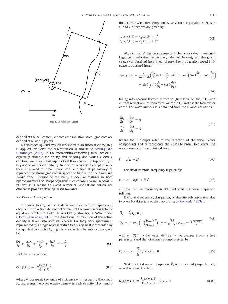
Fig. 1. Coordinate system.

1135D. Roelvink et al. / Coastal Engineering 56 (2009) 1133–1152

defined at the cell centers, whereas the radiation stress gradients aredefined at u- and v-points.

A first-order upwind explicit scheme with an automatic time stepis applied for flow; the discretization is similar to Stelling andDuinmeijer (2003), in the momentum-conserving form, which isespecially suitable for drying and flooding and which allows acombination of sub- and supercritical flows. Since the top priority isto provide numerical stability, first-order accuracy is accepted sincethere is a need for small space steps and time steps anyway, torepresent the strong gradients in space and time in the nearshore andswash zone. Because of the many shock-like features in bothhydrodynamics and morphodynamics we choose upwind schemati-zations as a means to avoid numerical oscillations which areotherwise prone to develop in shallow areas.

3.2. Wave-action equation

The wave forcing in the shallow water momentum equation isobtained from a time dependent version of the wave-action balanceequation. Similar to Delft University's (stationary) HISWA model(Holthuijsen et al., 1989), the directional distribution of the actiondensity is taken into account whereas the frequency spectrum isrepresented by a single representative frequency, best represented bythe spectral parameter fm,−1,0. The wave-action balance is then givenby:

∂A∂t +

∂cxA∂x +

∂cyA∂y +

∂cθA∂θ = −Dw

σð0:1Þ

with the wave action:

Aðx; y; t; θÞ = Swðx; y; t; θÞσðx; y; tÞ ð0:2Þ

where θ represents the angle of incidence with respect to the x-axis,Sw represents the wave energy density in each directional bin and σ

the intrinsic wave frequency. The wave-action propagation speeds inx- and y-directions are given by:

cxðx; y; t; θÞ = cg cosðθÞ + uL

cyðx; y; t; θÞ = cg sinðθÞ + vLð0:3Þ

With uL and vL the cross-shore and alongshore depth-averagedLagrangian velocities respectively (defined below), and the groupvelocity cg obtained from linear theory. The propagation speed in θ-space is obtained from:

cθðx; y; t; θÞ =σ

sinh 2kh∂h∂x sin θ−∂h

∂y cos θ� �

+ cosθ sin θ∂u∂x− cos θ

∂u∂y

� �

+ sinθ sin θ∂v∂x− cos θ

∂v∂y

� �ð0:4Þ

taking into account bottom refraction (first term on the RHS) andcurrent refraction (last two terms on the RHS) and h is the total waterdepth. The wave number k is obtained from the eikonal equations:

∂kx∂t +

∂ω∂x = 0

∂ky∂t +

∂ω∂y = 0

ð0:5Þ

where the subscripts refer to the direction of the wave vectorcomponents and ω represents the absolute radial frequency. Thewave number is then obtained from:

k =ffiffiffiffiffiffiffiffiffiffiffiffiffiffiffiffiffik2x + k2y

qð0:6Þ

The absolute radial frequency is given by:

ω = σ + kxuL + kyv

L ð0:7Þ

and the intrinsic frequency is obtained from the linear dispersionrelation.

The total wave energy dissipation, i.e. directionally integrated, dueto wave breaking is modelled according to Roelvink (1993a);

Dw =απQbσEw

Qb = 1− exp − Hrms

Hmax

� �n� �; H =

ffiffiffiffiffiffiffiffiffi8Ewρg

s; Hmax = γ tanhkh

k

ð0:8Þ

with α=O(1), ρ the water density, γ the breaker index (a freeparameter) and the total wave energy is given by:

Ewðx; y; tÞ = ∫2π

0

Swðx; y; t; θÞdθ: ð0:9Þ

Next the total wave dissipation, D , is distributed proportionallyover the wave directions:

Dwðx; y; t; θÞ =Swðx; y; t; θÞEwðx; y; tÞ

Dwðx; y; tÞ ð0:10Þ


This closes the set of equations for the wave-action balance. Giventhe spatial distribution of the wave action and therefore wave energythe radiation stresses can be evaluated (using linear wave theory):

Sxx;wðx; y; tÞ = ∫cgcð1 + cos2 θÞ−1

2

� �Swdθ

Sxy;wðx; y; tÞ = Syx;w = ∫ sinθ cosθcgcSw

� �dθ

Syy;wðx; y; tÞ = ∫cgcð1 + sin2 θÞ−1

2

� �Swdθ

ð0:11Þ

3.3. Roller energy balance

The roller energy balance is coupled to the wave-action/energybalance where dissipation of wave energy serves as a source term forthe roller energy balance. Similar to the wave action the directionaldistribution of the roller energy is taken into account whereas thefrequency spectrum is represented by a single mean frequency. Theroller energy balance is then given by:

∂Sr∂t +

∂cxSr∂x +

∂cySr∂y +

∂cθSr∂θ = −Dr + Dw ð0:12Þ

with the roller energy in each directional bin represented by Sr(x,y,t,θ).The roller energy propagation speeds in x- andy-directions are given by:

cxðx; y; t; θÞ = c cosðθÞ + uL

cyðx; y; t; θÞ = c sinðθÞ + vLð0:13Þ

The propagation speed in θ-space is identical to the expressionused for the wave energy density propagation (Eq. (0.4)), thusassuming that waves and rollers propagate in the same direction. Thephase velocity is obtained from linear wave theory:

c =σk

ð0:14Þ

The total roller energy dissipation is given by (Reniers et al., 2004a):

Dr =2gβrEr

cð0:15Þ

which combines concepts by Deigaard (1993) and Svendsen (1984).Next the total roller dissipation, D r, is distributed proportionally

over the wave directions:

Drðx; y; t; θÞ =Srðx; y; t; θÞErðx; y; tÞ

Drðx; y; tÞ ð0:16Þ

This closes the set of equations for the roller energy balance.The roller contribution to radiation stress is given by:

Sxx;rðx; y; tÞ = ∫ cos2θSrdθ

Sxy;rðx; y; tÞ = Syx;rðx; y; tÞ = ∫ sinθ cosθSrdθ

Syy;rðx; y; tÞ = ∫ sin2θSrdθ:

ð0:17Þ

These roller radiation stress contributions are added to the wave-induced radiation stresses (Eq. (0.11)) to calculate the wave forcingutilizing the radiation stress tensor:

Fxðx; y; tÞ = −∂Sxx;w + Sxx;r

∂x +∂Sxy;w + Sxy;r

∂y

!

Fyðx; y; tÞ = −∂Sxy;w + Sxy;r

∂x +∂Syy;w + Syy;r

∂y

!:

ð0:18Þ

3.4. Shallow water equations

For the low-frequency and mean flows we use the shallow waterequations. To account for the wave-induced mass flux and thesubsequent (return) flow these are cast into a depth-averagedGeneralized Lagrangian Mean (GLM) formulation (Andrews andMcIntyre, 1978, Walstra et al., 2000). In such a framework, themomentum and continuity equations are formulated in terms of theLagrangian velocity, uL, which is defined as the distance a waterparticle travels in one wave period, divided by that period. Thisvelocity is related to the Eulerian velocity (the short-wave-averagedvelocity observed at a fixed point) by:

uL = uE + uS and vL = vE + vS: ð0:19Þ

Here uS, vS represent the Stokes drift in x- and y-directionsrespectively (Phillips, 1977):

uS =Ew cosθρhc

and vS =Ew sinθρhc

ð0:20Þ

where the wave-group varying short-wave energy and direction areobtained from the wave-action balance (Eq. (0.1)). The resultingGLM-momentum equations are given by:

∂uL

∂t + uL ∂uL

∂x + vL∂uL

∂y −fvL−νh∂2uL

∂x2+

∂2uL

∂y2

!

=τsxρh

−τE

bx

ρh−g

∂η∂x +

Fxρh

ð0:21Þ

∂vL

∂t + uL ∂vL

∂x + vL∂vL

∂y + fuL−νh∂2vL

∂x2+

∂2vL

∂y2

!

= +τsyρh

−τE

by

ρh−g

∂η∂y +

Fyρh

ð0:22Þ

∂η∂t +

∂huL

∂x +∂hvL

∂y = 0: ð0:23Þ

Here τbx, τby are the bed shear stresses, η is the water level, Fx, Fyare the wave-induced stresses, νt is the horizontal viscosity and f isthe Coriolis coefficient. The bottom shear stress terms are calculatedwith the Eulerian velocities as experienced by the bed:

uE = uL−uS and vE = vL−vS ð0:24Þ

and not with the GLM velocities. Also, the boundary condition for theflow computations is expressed in functions of (uL, vL) and not (uE, vE).

3.5. Sediment transport

The sediment transport is modelled with a depth-averagedadvection diffusion equation (Galappatti and Vreugdenhil, 1985):

∂hC∂t +

∂hCuE

∂x +∂hCvE

∂y +∂∂x Dhh

∂C∂x

� �+

∂∂y Dhh

∂C∂y

� �=

hCeq−hCTsð0:25Þ

where C represents the depth-averaged sediment concentrationwhich varies on the wave-group time scale, and Dh is the sedimentdiffusion coefficient. The entrainment of the sediment is represented


by an adaptation time Ts, given by a simple approximation based onthe local water depth, h, and sediment fall velocity ws:

Ts = max 0:05hws

;0:2� �

s ð0:26Þ

where a small value of Ts corresponds to nearly instantaneoussediment response. The entrainment or deposition of sediment isdetermined by the mismatch between the actual sediment concen-tration, C, and the equilibrium concentration, Ceq, thus representingthe source term in the sediment transport equation.

The bed-updating is discussed next. Based on the gradients in thesediment transport the bed level changes according to:

∂zb∂t +

fmor

ð1−pÞ∂qx∂x +

∂qy∂y

!= 0 ð0:27Þ

where p is the porosity, fmor is a morphological acceleration factor of O(1–10) (e.g. Reniers et al., 2004a) and qx and qy represent thesediment transport rates in x- and y-directions respectively, given by:

qxðx; y; tÞ =∂hCuE

∂x

" #+

∂∂x Dhh

∂C∂x

� �� ð0:28Þ

and

qyðx; y; tÞ =∂hCvE

∂y

" #+

∂∂y Dhh

∂C∂y

� �� : ð0:29Þ

3.6. Transport formulations

The equilibrium sediment concentration can be calculated withvarious sediment transport formulae. At the moment the sedimenttransport formulation of Soulsby–van Rijn (Soulsby, 1997) has beenimplemented. The Ceq is then given by:

Ceq =Asb + Ass

hjuE j2 + 0:018

u2rms

Cd

!0:5

−ucr

!2:4

ð1−αbmÞ ð0:30Þ

where sediment is stirred by the Eulerian mean and infragravityvelocity in combination with the near bed short-wave orbital velocity,urms, obtained from the wave-group varying wave energy using linearwave theory. The combined mean/infragravity and orbital velocityhave to exceed a threshold value, ucr, before sediment is set in motion.The drag coefficient, Cd, is due to flow velocity only (ignoring short-wave effects). To account for bed-slope effects on the equilibriumsediment concentration a bed-slope correction factor is introduced,where the bed slope is denoted by m and αb represents a calibrationfactor. The bed load coefficients Asb and the suspended load coefficientAss are functions of the sediment grain size, relative density of thesediment and the local water depth (see Soulsby, 1997 for details).

3.7. Avalanching

To account for the slumping of sandy material during storm-induced dune erosion avalanching is introduced to update the bedevolution. Avalanching is introduced when a critical bed slope isexceeded:

j ∂zb∂x j > mcr ð0:31Þ

with a similar expression for the y-direction. Here we consider thatinundated areas are much more prone to slumping and therefore weapply separate critical slopes for dry andwet points; default values are

1 and 0.3, respectively. The former value is consistent with theequilibrium profile according to Vellinga (1986); it is higher than theangle of natural repose andmust be seen as an average slope observedafter dune erosion, where some stretches may exhibit vertical slopesand other, drier parts may have slumped further. The underwatercritical slope is much lower, and our estimate is based on themaximum underwater slopes we have observed in experiments, e.g.the Zwin test (see below) and tests carried out at Oregon StateUniversity with initially rather steep profiles.

When the critical slope between two adjacent grid cells isexceeded, sediment is exchanged between these cells to the amountneeded to bring the slope back to the critical slope. This exchange rateis limited by a user-specified maximum avalanching transport rate,which for sandy environments is usually set so high as to have noinfluence on the outcome, while ensuring numerical stability.

In our model simulations, the avalanching mechanism is typicallytriggered when a high infragravity wave reaches the dune front andpartly inundates it. The critical underwater slope is suddenlyexceeded and the two grid cells at the dune foot are adjusted duringthe first timestep when this happens. In subsequent timesteps a chainreaction may take place both in points landward, where now thecritical dry slope may be exceeded because of the lowering of the lastwet point, and in points seaward, where now the critical wet slopemay be exceeded. As a result, sediment is brought from the dry duneinto the wet profile, where it is transported further seaward byundertow and infragravity backwash. An essential difference withsimilar procedures in other dune erosion models is the fact thatavalanching is only applied between adjacent grid cells, rather thanextrapolating profile behaviour well beyond the wet domain. This ismade possible by explicitly resolving the long-wave swash motions.Another big advantage with respect to existing procedures is that thesimple avalanching algorithm is readily applied in two dimensions.

3.8. Wave boundary conditions

For the waves the wave energy density at the offshore boundary isprescribed as a function of y, θ and time. This can be generated forgiven spectral parameters or using directional spectrum information.Themethod is based on the theory of Hasselmann (1962) (c.f. Herberset al., 1994), previously implemented and used by Van Dongeren et al.(2003) to model infragravity waves in the nearshore. At the lateralboundaries, for wave components entering the domain, the along-shore or along-crest gradient is set to zero, effectively eliminating thenotorious ‘shadow zones’ found in many wave models.

3.9. Flow boundary conditions

At the seaward and landward (in case of a bay) boundary radiatingboundary conditions are prescribed, taking into account the incomingbound long waves, following Van Dongeren and Svendsen (1997a).

For the lateral boundaries so-called Neumann boundaries are used,where the longshorewater level gradient is prescribed, in this case setto zero. This type of boundary conditions has been shown to workquite well with (quasi-)stationary situations, where the coast can beassumed to be uniform alongshore outside the model domain. So farwe have found that also in case of obliquely incident wave groups thiskind of boundary conditions appears to give no large disturbances,although it takes some alongshore distance for edge waves and shearwaves to be fully developed.

4. Model verification cases

To verify the implementation and validate the model approachdescribed in Section 3 a number of test cases have been carried out,both in 1D and in 2DH mode. The first series of tests focuses on thedescription of the wave-group induced hydrodynamics, swash


dynamics, sediment transports and concurrent bed evolution in a one-dimensional setting. Tests include both laboratory and field cases toexamine the general validity of the modelling with emphasis on bothswash dynamics and avalanching. Next a number of tests areperformed including the alongshore dimension. These 2D modetests include analytical and field cases with alongshore variability inthe forcing and/or the bathymetry. All tests have been performedwitha standard set of parameter settings (see Appendix A) unless statedotherwise. In addition, for all tests the model performance wasquantified by determining error parameters for the modelledhydrodynamics and morphodynamics, which are listed in Table 1.

The model validation commences with 1D large-scale duneerosion test (Arcilla et al., 1994), validating short-wave and long-wave motions as well as the sediment transport and profile evolutionin well-controlled conditions. Next a more recent test with combineddune erosion and overtopping is examined (van Gent et al., 2008)showing again that inner surf hydrodynamics, sediment transportsand profile evolution are well represented. This is followed by a seriesof field-scale tests of dune erosion and overwashing on differentprofiles that are compared with observations reported by Jiménezet al. (2006) after Assateague Island was hit by two northeasters in1998. Next a number of tests are performed including the alongshoredimension. Starting with a two-dimensional case of long-wave runup(Zelt, 1986), followed by comparisons with field measurements atDuck, NC during the Delilah field experiment to show the ability of themodel to capture two-dimensional hydrodynamic processes on a realbeach. Finally the process of breaching is tested against a prototypefield experiment reported by Visser (1998).

4.1. LIP11D delta flume 1993—test 2E

This model test, described in Arcilla et al. (1994), concernsextreme conditions with a raised water level at 4.58 m above theflume bottom, a significant wave height, Hm0, of 1.4 m and peakperiod, Tp, of 5s. Bed material consisted of sand with a D50 ofapproximately 0.2 mm. During the test substantial dune erosion tookplace.

Based on the integral wave parameters Hm0 and Tp and a standardJonswap spectral shape, time series of wave energy were generatedand imposed as boundary condition. Since the flume tests werecarried out with first-order wave generation (no imposed super-harmonics and sub-harmonics), the hindcast runs were carried outwith the incoming bound long waves set to zero (‘first-order wavegeneration’). Active wave reflection compensation was applied in thephysical model, which has a result similar to the weakly reflectiveboundary condition in XBeach, namely to prevent re-reflecting ofoutgoing waves at the wave paddle (offshore boundary).

A grid resolution of 1 m was applied and the sediment transportsettings were set at default values, see Appendix A. For themorphodynamic testing the model was run for 0.8 h of hydrodynamictime with a morphological factor of 10, effectively representing amorphological simulation time of 8 h.

Table 1Definition of error parameters.

Parameter Formula (m=measured, c=computed) Remarks

Correlation coefficient R2 Covðm; cÞσmσc

R2=1 means no sc

Scatter index SCI rms c−m

maxðrmsm ; j<m> j ÞThis is a relative memaximum of the rmresults for data wit

Relative bias< c−m >

maxðrmsm; j < m > j Þ This is a relative me

Brier Skill Score BSS 1−Varðc−mÞVarðmÞ

This parameter reladata. BSS=1 meanscenario. We consid

Test results are given for the root mean square wave height, Hrms,and the root mean square orbital velocity, Urms, separated in high-frequency (frequencies above fp/2 corresponding to incident waves)and low-frequency parts (corresponding to infragravity waves). InXBeach model terms, these parameters are defined as follows:

Hrms;HI =ffiffiffiffiffiffiffiffiffiffiffiffiffiffiffiffi< H2 >

pð0:32Þ

urms;HI =ffiffiffiffiffiffiffiffiffiffiffiffiffiffiffiffiffiffiffiffi< u2

rms >

q; urms =

1ffiffiffi2

p πHTp sinhðkhÞ

ð0:33Þ

Hrms;LO =ffiffiffiffiffiffiffiffiffiffiffiffiffiffiffiffiffiffiffiffiffiffiffiffiffiffiffiffiffiffiffiffiffiffiffiffiffiffiffiffiffiffi8 < ðη− < η >Þ2 >

qð0:34Þ

urms;LO =ffiffiffiffiffiffiffiffiffiffiffiffiffiffiffiffiffiffiffiffiffiffiffiffiffiffiffiffiffiffiffiffiffiffiffiffiffiffiffiffiffiffi< ðuL− < uL >Þ2 >

q: ð0:35Þ

In Fig. 2 the results are shown both for first-order wave generation(as in the flume tests) and for second-order wave generation(including incoming bound long waves). The model is clearly capableof capturing both the HF and LF wave heights and orbital velocities; italso shows the effect of second-order wave generation on the LFwaves. For this test, the agreement is indeed better if incoming boundlong waves are omitted from the flow boundary condition (as theywere in the laboratory test).

In Fig. 3 the horizontal distribution of sedimentation and erosionafter 8 h is shown, and the evolution in time of the erosion volumeand the dune retreat, again both for first-order wave generation (as inthe physical test) and for second-order steering. For the correctsteering, we see a good agreement for all three parameters.Noteworthy is the episodic behaviour of the dune erosion, both inmeasurements and model, although the almost exact (deterministic)reproduction of the (stochastic) dune retreat must be a coincidence.An important conclusion for physical model tests is that for duneerosion it does make a difference whether first-order or second-orderwave steering is applied.

A key element in the modelling is the avalanching algorithm; eventhough surfbeat waves running up and down the upper beach are fullyresolved by the model, without a mechanism to transport sand fromthe dry dune face to the beach the dune face erosion rate issubstantially underestimated. The relatively simple avalanchingalgorithm described above, whereby an underwater critical slope of0.3 and a critical slope above water of 1.0 are applied, proves to bequite successful in representing the retreat of the upper beach anddune face. In Fig. 4 the measured and modelled bed evolution areshown, which looks quite good in the upper region. In contrast, Fig. 5shows the results of two simulations where either the avalanchingmechanism (left panel) or the infragravity wave motion (right panel)were left out. Both cases show significant underprediction of the duneerosion, which demonstrates the need to have both processesincluded in the model.

Error statistics for the standard run are collected in Table 5, andgenerally show a scatter index and relative bias of less than 10% for

atter, tendency may still be wrong

asure of the scatter between model and data. The error is normalized with thes of the data and the absolute value of the mean of the data; this avoids strange

h small mean and large variabilityasure of the bias, normalized in the same way as the Scatter Index.

tes the variance of the difference between data and model to the variance of thes perfect skill, BSS=0 means no skill, BSS<0 means model is worse than ‘no change’er this parameter mainly to judge the skill of the sedimentation/erosion patterns

Fig. 2. Computed and observed hydrodynamic parameters for test 2E of the LIP11D experiment. Top left: bed level and mean water level. Top right: measured (dots) and computedmean water level with first-order steering (drawn line) and second-order steering (dashed line) as a function of the cross-shore distance. Middle left: same for HF wave height;middle right: same for LF wave height; bottom left: same for HF orbital velocity; bottom right: same for LF orbital velocity.


the hydrodynamic parameters and overall erosion volumes and duneretreat. An exception is themean velocity, for which the higher scatterand bias can be attributed to the (neglected) 3D structure of thisparameter. The horizontal distribution of the sedimentation anderosion at the end of the test shows a higher scatter, determined inpart by the areas with small changes; the Brier Skill Score shows avalue of 0.72, which for morphodynamic models is considered good(Van Rijn et al., 2003).

Fig. 3. Computed and observed sedimentation and erosion after 8 hrs (top panel); erosion vtime for test 2E of the LIP11D experiment, (Arcilla et al., 1994). All results with first-order

4.2. Deltaflume 2006

We continue with a more recent test of a more complex profile(van Gent et al., 2008, test T4) in which a small dune in front of a largevolume dune is breached (see Fig. 6). In addition, a sand mining pit ispresent in the profile at x=65 m, which is believed to have littleinfluence on the nearshore dynamics and the amount of dune erosion.This test is the best controlled case with dune overwash known to us.

olume as function of time (bottom left) and dune retreat (bottom right) as function ofsteering (drawn line) and second-order steering (dashed line).

Fig. 4. Measured and modelled bed level after 1, 2, 4 and 8 h of wave action, for a water level of 4.56 m above the flume bottom.


The test duration is 6 h and profile measurements were obtained after0.l, 0.3, 1.0, 2.0 and 6.0 h. Also detailed measurements of wavetransformation, near dune flows and sediment concentrations areavailable for comparing with model results. In the physical model testthe still water level was set at 4.5 m above the flume's floor andimposed wave conditions correspond to a Pierson–Moskowitzspectrum with Hm0=1.5 m and Tp=4.90 s. The wave paddle wasoperated with active wave reflection and second-order steering.Further details may be found in Van Gent et al., 2008 and Van Thiel deVries et al., 2008.

The simulation is performed for 6 h on a uniform grid in which thegrid size Δx is set at 1 m. In order to make a detailed comparisonbetween measured and simulated hydrodynamics over the develop-ing profile, the simulation is carried out with a morphological factor of1. The offshore model boundary is located at 41 m from the waveboard and we use measured water surface elevations and flowvelocities at this location to obtain time series of the incident waveenergy and the incoming bound long-wave water surface elevations.Other model settings are the same as for test 2E of the LIP11Dexperiment and are listed in Appendix A.

Fig. 6 compares the modelled and observed profile evolution. Bothmodel and data first show a scarping of the profile, a brief period ofoverwashing followed by a smoothing out of the remainder of the

Fig. 5. Measured (drawn line) and modelled (dashed line) profile after 8 h o

berm and a renewed attack on the actual dune face, which is slow asmost of the wave energy dissipates on the shallow upper profile leftby the berm. The modelled profile evolution appears to be slightlyslower than observed and also at the end of the test the modelledupper profile is slightly too low, which could be due to lack of onshoresediment transports.

Test averaged hydrodynamic parameters are compared in Fig. 7 andreveal a good agreement betweenmeasured and simulatedwave heighttransformation for both incident and long waves (upper left panel), thewave orbital flows for both incident and longwaves (upper right panel)and the time and depth-averaged return flow (lower right panel). It isremarked that the measured time and depth-averaged flows just infront of the dune (at x=205 m) should be interpretedwith care since inthe physical model only limited observation points over depth areavailable (Van Thiel de Vries et al., 2008).

Error statistics are collected in Table 5, and generally show ascatter index and relative bias of less than 10% for the hydrodynamicparameters and overall erosion volumes and dune retreat. Anexception is the mean velocity, for which the higher scatter and biascan be attributed to the (neglected) 3D structure of this parameter.The horizontal distribution of the sedimentation and erosion at theend of the test shows a bit higher scatter, determined in part by theareas with small changes; the Brier Skill Score shows a value of 0.98.

f wave action, left panel: no avalanching; right panel: no wave groups.

Fig. 6. Deltaflume 2006 test T04. Measured (drawn lines) and modelled (dashed lines) profile after 0, 0.1, 0.3, 1, 2 and 6 h of wave action.


Amore detailed analysis of the hydrodynamics is given in Figs. 8 and9 which compare measured and simulated wave spectra and watersurface elevation time series respectively. It is remarked that themeasured wave spectra and water surface elevations include both theincident waves and long waves whereas the simulation results areassociated with (wave-group generated) long waves only. Consideringthe wave spectra first, it is seen that themeasured wave spectra show ashift in variance towards lower frequencies as the waves propagate tothe dune face. At the offshore model boundary most of the measured

Fig. 7. Deltaflume 2006 test T04. Upper left panel: measured (markers) and simulated (linestotal (squares/solid line) wave height. Upper right panel: measured (markers) and simulatedline) time and depth-averaged flow velocity.

wavevariance is associatedwith incidentwaves and the simulated long-wave spectrum explains a marginal part of the measured wavespectrum. However, getting close to the dune face the incident wavevariance reduces due to depth induced breakingwhereas the long-wavevariance increases due to shoaling (Battjes et al., 2004). At the mostshoreward pressure sensor (about 10 m from the dune face)most of themeasuredwave variance is associatedwith longwaves and is favourablysimulated with the surfbeat model. The same phenomenon can beobserved in Fig. 9, which shows a reasonably good correlation

) LF (downward triangles/dashed–dotted line), HF (upward triangles/dashed line) and(lines) orbital flow velocity. Lower left panel: measured (squares) and simulated (solid

Fig. 8. Measured wave spectra including both incident waves and long waves (thin line) compared with simulated long-wave spectra (thick line) at different cross-shore positions(see upper left corner of sub-panels). Measured and simulated spectra are computed over the whole test duration.

Fig. 9. Measured water surface elevations including both incident and long waves (thin line) compared with simulated long-wave water surface elevations (thick line) at differentcross-shore positions (see lower left corner of sub-panels) after 4.17 wave hours.



(R2=0.32) between measured and simulated water surface elevationsclose to the dune face (lower right panel). Also the time series showsteep long-wave fronts indicating breaking as was shown in thebichromatic wave case by Van Dongeren et al. (2007).

A comparison given between the observed andmodelled sedimentconcentrations and sediment transports (Fig. 10) shows that themodel clearly underestimates the concentration near the dune face,whereas the sediment transport is somewhat overestimated. Theexplanation for this could be found in an overestimation of the neardune time and depth-averaged undertow which compensates forunderestimating the near dune sediment concentrations. Throughoutthe flume, the sediment transport is too much seaward, as no onshoreprocesses are included yet; work to improve this is currentlyunderway but beyond the scope of this paper. Simulated sedimenttransport gradients are favourably predicted by the model, whichresults in a response of the coastal profile that compares reasonablywell to the measurements.

4.3. Dune erosion and overwash field tests

Besides well-controlled laboratory cases, the model is also appliedto the field. The first example concerns the morphodynamic responseof sandy dunes to extreme storm impacts at Assateague Island,Maryland, USA, which was analyzed before by Jiménez et al. (2006).Two consecutive northeasters attacked the barrier island during lateJanuary and early February, 1998. The bathymetry was measuredusing LIDAR in September 1997 and again February 9th and 10th,1998 after the two storms had subsided.

Three types of dunes were identified by Jiménez et al. (2006),shown in Fig. 11. Profile A (upper left panel) is initially characterizedby a steep faced dune, where the maximum runup exceeded the dunecrest height and the mildly sloped back of the dune. The morpholog-ical response is characterized by profile lowering, decrease of thebeach face slope and landward barrier displacement, while retainingbarrier width.

Profile type B is a double-peaked dune profile and has twodifferent shapes. Profile B1 (upper right panel) is initially character-ized by a primary and secondary dune, both of which are lower than

Fig. 10. Deltaflume 2006. Test T04. Top panel: observed depth-averaged concentrations (sqevolution (drawn line) vs. model result (dashed line).

the maximum runup height and which are separated by a valley.Profile B2 (bottom left panel) initially has two peaks of which theseaward one is lower. The backside of the barrier of either type istherefore either characterized by a secondary dune line (profile B1) ora taller crest of the dune (profile B2) which prevents the eroded sandfrom being transported to the backside of the dune. The mainmorphological response for these profile types is a decrease of thebeach face slope, outer shoreline retreat and narrowing of the barrier.

The height of the dune crest of profile C (lower right panel)exceeds the maximum runup height and so little overwash isobserved. The morphological response of this type of profile is crestlowering due to slumping, decrease of the beach face slope and retreatof the outer shoreline. The width of the barrier is seen to decrease.

The storm impact of the two North Easters on Assateague Islandwas modelled with XBeach for the four profiles described by Jiménezet al. (2006). The profiles were extendedwith a shallow foreshore anda 1:100 slope in seaward direction till a water depth of 9 m belowNAVD88. As XBeach has not been shown to accurately simulatemorphological change during very long storm durations, the simula-tions were run for a total of 20 h. The measured wave and surgeconditions were parameterized for each storm by a constant surgelevel and a constant wave height and wave period (see Table 2). Thisapproach assumes that two 72 hour storms with varying surge andwave conditions can be approximated by two 10 hour simulationswith constant maximum surge and wave conditions following asimilar approach as Vellinga (1986). This approach also facilitatesfurther sensitivity studies into the effect of varying hydraulic forcingconditions. The calculation grid size varies from 18 m at the offshoreboundary to 2 m on the islands. A morphological acceleration factor of5 is applied. The final simulated bed profiles are shown in Fig. 11.

The profile changes calculated by XBeach are largely consistentwith the description of dune evolution given by Jiménez et al. (2006).Jiménez et al. observed that profile A became flatter, with largequantities of eroded sediment deposited on the back side of thebarrier island, due to the consistent wave overtopping. The modelreplicates this behaviour, except that the island is lowered more thanin the measurements and that the seaward face of the island does notroll back as it does in the measurements.

uares) vs. model result. Bottom panel: total sediment transport observed from profile

Fig. 11. Pre-storm profiles (black dotted line), measured post-storm profiles (black solid line) and modelled post-storm profiles (red solid line). Upper left panel: profile A. Upperright panel: profile B1. Lower left panel: profile B2. Lower right panel: profile C. The seaward side is on the left of all panels. Note that the measured post-storm profiles contain onlythe sea surface and emerged topography and no submerged topography.


The observed response of profile B1 was dune face retreat,overwash deposition in the dune valley between the primary andsecondary dunes and narrowing of the island, Jiménez et al. (2006)also noted decrease of the beach face slope. It can be seen in Fig. 11that the morphological development of the island is well representedby the model. The simulated dune crest retreat corresponds closely tothe measured retreat. Overwash takes place in the model andsediment is deposited in the valley between the primary andsecondary dunes, although the magnitude of deposition is less thanin the measurements.

The XBeach model of profile B2 shows a slope reduction on theseaward side and lowering of the seaward dune. The second dunecrest retains its crest level as described in the work of Jiménez et al.(2006). The beach slope decrease in the XBeach model is in line withthe description given by Jiménez et al. (2006), but differs from theirmeasured profile. It is unclear why themeasured profile shows almostno erosion of the beach face.

Jiménez et al. (2006) observed, in general, profile C to lower inheight, the seaward dune slope to become smaller, and seaside retreatof the shoreline resulting in barrier narrowing. The XBeach modelshows retreat of the upper dune face and a reduction of the seawarddune slope. The model overpredicts the sedimentation at the base ofthe dune and underpredicts the crest lowering.

Though the model reasonably predicts post-storm beach and dunetopography the results are obtained from a model that is based on

Table 2Hydrodynamic boundary conditions XBeach simulations.

Storm 1 Storm 2

Surge level [m]+NAVD 0.75 1.0Hs [m] 4.1 3.9Tp [s] 8.5 8.5Spectrum Pierson–Moskowitz Pierson–Moskowitz

several simplifications according to surge and wave conditions. Inaddition the underwater profile is unknown at the seaside and isschematized with a 1:100 slope. A quantitative comparison ofmodelled and measured profile evolution therefore has limitedvalidity; however we can conclude that the model has qualitativeskill in predicting overwash morphology.

In order to obtain more insight in the effect of these simplificationsand assumptions on the morphological response during the storms,additional simulations were performed with varying surge levels,wave conditions and foreshore slopes as listed in Table 3.

The sensitivity studies show that the variation in the morpholog-ical response of the profiles to the incident wave parameters andsurge level is dependent on the initial shape of the profile. Thissensitivity is most prominent in profile A (Fig. 12), in which overwashoccurs for much of the storm duration, and least in profile C (Fig. 13),in which only dune erosion takes place. This shows that more accuratehydraulic boundary conditions are required in order to correctlysimulate field cases with overwash than cases with dune erosion. Theparameterization of the hydraulic boundary conditions in this studyfollows an approach designed for dune erosion cases (Vellinga, 1986).The sensitivity cases suggest that this approach may not be applicableto overwash cases. Further research into storm schematisation foroverwash conditions is needed before the model can be consideredmore than qualitatively correct for overwash.

4.4. Zelt analytical 2DH runup case

All the verification cases so far considered solely the cross-shoredimension and assumed a longshore uniform coast. In the followingcases the potential of the model to predict coastal and dune erosion insituations that include the 2 horizontal dimensions is furtherexamined. A first step towards a 2DH response is to verify that the2DH forcing by surge runup and rundown is accurately modelled. Thisaccuracy is controlled by the flooding and drying criterion. Thiscriterion is tested against a numerical solution for the runup of a

Table 3Sensitivity cases.

Base S1 S2 S3 S4 S5 S6 S7 S8

Surge level [m]+NAVD (%) 100 125 75 100 100 100 100 100 100Hs [m] (%) 100 100 100 125 75 100 100 100 100Tp [s] (%) 100 100 100 100 100 125 75 100 100Foreshore slope 0.01 0.01 0.01 0.01 0.01 0.01 0.01 0.02 0.005

Fig. 12. Sensitivity of profile A to the incident wave height (top left panel), wave period (top right panel), surge level (bottom left panel) and foreshore slope (bottom right panel).The initial (dotted line) and final profile (solid line) of the base simulation are shown in all four panels. The difference between the final profile of the sensitivity simulation and thebase simulation is shown in light grey (for cases S2, S4, S6 and S8) or dark grey (for cases S1, S3, S5 and S7).

Fig. 13. Sensitivity of profile C to the incident wave height (top left panel), wave period (top right panel), surge level (bottom left panel) and foreshore slope (bottom right panel).The initial (dotted line) and final profile (solid line) of the base simulation are shown in all four panels. The difference between the final profile of the sensitivity simulation and thebase simulation is shown in light grey (for cases S2, S4, S6 and S8) or dark grey (for cases S1, S3, S5 and S7).


Fig. 14. Definition sketch of the concave beach bathymetry (courtesy of H.T. Őzkan-Haller).


solitary wave on a concave bay with a sloping bottom (Fig. 12) thatwas obtained by Őzkan-Haller and Kirby (1997), who used a Fourier–Chebyshev Collocationmodel of the nonlinear non-dispersive shallowwater equations. This solution is used rather than the originalsimulation by Zelt (1986), who used a fully Lagrangian finite elementmodel of the shallow water equations, which included somedissipative and dispersive terms which presently cannot be modelledin XBeach. The XBeach model is run without friction, short-waveforcing or diffusion.

Fig. 14 shows the definition sketch of the concave beachbathymetry in the present coordinate system, converted from theoriginal system by Zelt (1986). The bathymetry consists of a flatbottom part and a beach part with a sinusoidally varying slope. For

Fig. 15. Comparison of present model (solid) to Őzkan-Haller and Kirby (1997) (dashed): (respectively, and (b) maximum runup and rundown.

Zelt's (1986) fixed parameter choice of hs/Ly=4/(10π), the bathym-etry is given by

h =

hs ;x≤Ls

hs−0:4ðx−LsÞ

3−cosπyLy

! ;x > Ls

8>>>><>>>>:

ð0:36Þ

where hs is the shelf depth, Ls is the length of the shelf in themodelleddomain and Ly is the length scale of the longshore variation of thebeach. This results in a beach slope hx=0.1 in the center of the bayand of hx=0.2 normal to the “headlands”. In the following we choseLy=8 m, which determines hs=1.0182 m. We set Ls= Ly anddifferent values for Ls only cause phase shifts in the results, but noqualitative difference, so this parameter is not important in thisproblem. Also indicated in the figure are the five stations where thevertical runup (the surface elevation at the shoreline) will bemeasured.

At the offshore x=0 boundary we specify an incoming solitarywave, which in dimensional form reads

zs = αhs sech2

ffiffiffiffiffiffiffiffiffiffiffiffiffiffiffiffiffiffiffiffiffiffiffiffiffiffiffiffiffiffi3g4hs

αð1 + αÞs

ðt−t0Þ !

ð0:37Þ

which is similar to Zelt's (1986) Eq. (5.3.7) except that we neglect thearbitrary phase shift. The phase shift t0 is chosen such that the surfaceelevation of the solitary wave at t=0 is 1% of the maximumamplitude. The only parameter yet to be chosen is α. We will compareour model to Zelt's case of α = H

hs= 0:02 where H is the offshore

wave height. Zelt found that the wave broke for a value of α=0.03, sothe present test should involve no breaking, but has a large enoughnonlinearity to exhibit a pronounce two-dimensional runup.

Any outgoing waves will be absorbed at the offshore boundary bythe absorbing–generating boundary condition. At the lateral bound-aries y=0 and y=2 Ls we specify a no-flux (wall) boundary condition

a) time series of runup in 5 stations from top to bottom y/Ly=1, 0.75, 0.5, 0.25 and 0


following Zelt. The numerical parameters are Δx=Δy=0.125 mwitha Courant number of 0.7.

Fig. 15a shows the vertical runup ζ normalized with the offshorewave height H as a function of time, which is normalized byT =

ffiffiffiffiffiffiffighs

p= Ly at the 5 cross-sections indicated in Fig. 14. The solid

lines represent the present model results while the dashed linesdenote Őzkan-Haller and Kirby's (1997) numerical results. We seethat the agreement is generally good, except that the present modeldoes not capture the second peak in the time series at y/Ly=1 verywell. This secondary peak or “ringing” is due to the wave energy thatis trapped along the coast and propagates towards themidpoint of thebay (Zelt, 1986). It is suspected that this focusing mechanism is notproperly captured, because the present method approximates theshoreline as a staircase pattern, which in effect lengthens theshoreline. Also, the spatial derivatives are not evaluated parallel andperpendicular to the actual shoreline but in the fixed x and ydirections. The agreement at locations y/Ly=0.25, y/Ly=0 0.5 and y/Ly=0.75 is generally good despite the large gradient of the localshoreline relative to our grid. The statistical overall score for the timeseries is R2=0.986, SCI=0.170 and the relative bias=0.009.

Note that Őzkan-Haller and Kirby (1997) use a moving, adaptinggrid with a fixed Δy (which is equal to the present model's Δy in thiscomparison) but with a spatially and temporally varying Δx so thatthe grid spacing near the shoreline is very small. In the present modelΔx is set equal to Δy, which means that we can expect to have lessresolution at the shoreline than Őzkan-Haller and Kirby (1997).

Fig. 15b shows the maximum vertical runup and rundown,normalized by H, versus the alongshore coordinate y. It is seen thatthe maximum runup agrees well with Őzkan-Haller and Kirby (1997)but that the maximum rundown is not represented well in the centerof the domain. The ‘wiggles’ in the solid line are evidence of thestaircasing of the shoreline: since the shoreline is not treated as acontinuous but rather as a discrete function, so is the runup in the

Fig. 16. Delilah field experiment 1990. Top panel: plan view of the model location and meameasurement gauge array (circles) and measurement gauge names.

individual nodes. The statistical score for the maximum runup isR2=0.98, SCI=0.04 and the relative bias=−0.03.

The above results are consistent with the results obtained with theSHORECIRCmodel which is based on similar hydrodynamic equations,see Van Dongeren and Svendsen (1997b), and show that also thecurrent model is capable of representing runup and rundown.

4.5. Delilah

In order to verify the 2DH hydrodynamics of XBeach forced bydirectionally-spread shortwaves a simulation is set up to comparemodelresults to fieldmeasurements. In this case the Delilah field experiment atDuck,NorthCarolina is selected as a suitable test location. Theperiod thatis modelled is October 13th 1990, which was a stormy day, between16:00 and 17:00 h. The significant wave height at 8 m water depth was1.81 m, with a peak period of 10.8 s and a mean angle of incidence of−16° relative to the shoreward normal. This period is selected becausethe wave conditions are energetic enough to generate a significantinfragravity wave component and the incident wave spectrum issufficiently narrow-banded to justify the assumptions in the modelboundary conditions. The model is forced with the wave spectrummeasured at 8 mwater depth (Birkemeier et al., 1997). Ameasured tidalsignal is imposed on the model boundaries of which the mean level is0.69 m above datum. The slope of the wave front in the roller model β isset to the default value of 0.10. A constant grid size of 5 m in cross-shoreand 10 m in longshore direction is used. The resolution of the wavemodel in directional space is 15°. The model is set to generate output atthe location of the primary cross-shore measurement array, gaugenumbers 10, 20, 30, 40, 50, 60, 70, 80 and 90 (Fig. 16).

The modelled time-averaged wave heights of the short waves arecompared to the time-averagedwave heights measured at the gauges.These results are shown in the first panel of Fig. 17. Unfortunately, nodata exist for gauge number 60.

surement gauge array (circles). Bottom panel: cross-shore profile at the location of the

Fig. 17. Delilah 1990: First panel: time-averaged measured (squares) and modelled (line) RMS-wave height of the short waves. Second panel: time-averaged measured (squares)and modelled (line) RMS-wave height of the infragravity waves. Third panel: time-averaged measured (squares) and modelled (line) longshore velocity. Fourth panel: cross-shoreprofile at the location of the measurement gauge array with the positions of the gauges (crosses).


The infragravity wave height is calculated as follows (van Dongerenet al., 2003):

Hrms;low =

ffiffiffiffiffiffiffiffiffiffiffiffiffiffiffiffiffiffiffiffiffiffiffiffi8 ∫

0:05Hz

0:005Hz

Sdf

vuut ð0:38Þ

Fig. 18. Delilah 1990: Measured (solid line) and modelled (dashed line) surface elevation sp

As can be seen in the second panel of Fig. 17, the XBeach modelunderestimates the infragravity wave height, but does follow themeasured cross-shore trend well.

The measured and modelled time-averaged longshore current isshown in the third panel of Fig. 17. It can be seen that the modelstrongly underpredicts the longshore current in the trench between

ectra for nine locations in the primary cross-shore array. Gauge 90 is the most seaward.


measurement gauge 60 and the shore. Further calibration of the shortwave and roller parameters is required in order to improve thesimulated longshore current in this trough. The correlation coefficient,scatter index, relative bias and Brier Skill Score for the simulation areshown in Table 5. Results are somewhat sensitive to the choice ofroller parameter β.

The modelled and measured sea surface elevation spectra at allnine gauge locations are shown in Fig. 18. Note that similar to Fig. 8the modelled surface elevation spectra only contain low-frequencycomponents associated with wave groups. The figure shows amigration of energy from high to low frequencies in shorewarddirection in the measured spectra. The simulated spectra reproducewell the trend of increasing energy in the low-frequency band inshoreward direction, but the amount of energy in the simulated low-frequency band is less than in the measurements. In conclusion it canbe stated that the model reproduces to a high degree of accuracy theshort-wave transformation in the shoaling and breaker zone. Thetransfer of energy from high to low frequencies in the model hasqualitative skill. The longshore velocity in the nearshore requiresadditional calibration of the short wave and roller parameters.

Fig. 19. Sequence of 3D visualizations of the breach during the Zwin test (Visser, 1998). Be

4.6. ZWIN breaching test (Visser, 1998)

Having examined two-dimensional hydrodynamics, we move to2D morphodynamics. The next test carried out is that on the Zwinbreach growth experiment, as reported by Visser (1998). In themouthof the Zwin, a tidal inlet located at the border between theNetherlands and Belgium, an artificial dam was constructed with acrest height of 3.3 m+N.A.P. (Dutch datum, approx. MSL), crest width8 m, inner slope 1:3 outer slope 1:1.6 and length 250 m. An initialdepression of 0.8 m was made in the middle of the dam having awidth of 1 m and a side-slope of 1:1.6 to ensure that the breachinitiated at this location. The level of the surrounding sea bed wasabout 0.7 m+N.A.P. The mean tidal prism of the Zwin is about350,000 m3. The polder area Ap as a function of the water level behindthe dam zs is given by:

Ap = ð170;000mÞzs−100;000m2;0:60m < zs < 2:3m + N:A:P:

Ap = ð2;100;000mÞzs−4;540;000m2; zs≥2:3m + N:A:P:

ð0:39Þ

d level, water level and development of breach width (dots: observation, line: model).

Table 4Error statistics for breach width development during the Sensitivity runs of the Zwintest.

Run Description R2 SCI Rel. bias

r00 Default settings 0.94 0.09 −0.06r01 No bed-slope effect 0.88 0.44 −0.39r02 Chezy=50 √m/s instead of 65 √m/s 0.94 0.19 −0.16r03 Dryslp=0.6 instead of 1 0.93 0.19 −0.17r04 Wetslp=0.15 instead of 0.3 0.92 0.86 0.81r05 D50=0.2 mm instead of 0.3 mm 0.94 0.10 0.01r06 Adaptation timescale=0.2 s instead of 0.1 s 0.94 0.28 −0.23


At t=0, about 10 min prior to high water, the water level at theseaside was NAP+2.72 m. At t=10 min a water level of 2.75 m+N.A.P. was reached. For the remainder of the test, which had a totalduration of 1 h, the water level marginally decreased. After 1 thebreach growth became nil, as the water level of the polder area behindthe breached equaled the sea level. The wave height near the damwasnegligible during the experiment. The wind speed was about 2 m/s.

Until t=6.5 min the breach depth grewwhereas the breach widthremained constant. At t=6.5 min the original dike structure hadnearly completely disappeared over the initial depression width of1 m. Near t=6.5 min the onset of lateral breach growthwas observed.The scour hole developed further down to a depth of 1.6 m–N.A.P.(4.9 m below the original dam crest level). The rate of lateral breachgrowth was about 2 cm/s. After approximately 40 min the processslowed down considerably and after approximately 1 h the waterlevels at both sides were equal.

A schematized representation of theZwin testwas created inXBeach,with at the sea side a uniform bed level at 0.7 m+NAP, and inside thebasin a prismatic profile with the deepest point at 0.7 m+NAP andsloping sides, such that the polder area as a function of the water levelwas in accordance with Eq. (0.39). The grid is non-equidistant with gridsizes gradually varying from 0.5 m near the breach to approx. 50 m faraway from it. Themedian grain diameterD50 of the bedmaterial was setto 0.3 mm in accordance with the prototype test conditions for theartificial dam. The applied critical slopes for avalanching are the same asin other tests and standard settings were applied for the transportformulations (see Appendix A for default model settings). Waves werenegligible in the test andwere set to zero. Themodel was runwith a CFLof 0.5 and remained smooth and stable despite the steep slopes andsupercritical flows.

In Fig. 19 a sequence of 3D images is shown depicting the variousstages in the breaching process: the initial overflowing, the cuttingback of the breach, the deepening and finally the widening of thebreach. Qualitatively and quantitatively the results are in agreementwith the experiment by Visser (1998), although details may bedifferent due to the schematized initial bathymetry.

In Fig. 20 a comparison is given between measured and simulatedwater levels, flow velocities and development of the breach width intime. Observation point MS2 is 30 m upstream of the center point of

Fig. 20. Zwin test (Visser, 1998). Observed (drawn lines) and modelled (dashed lines) time sof breach width, observations (dots) vs. model (drawn line).

the breach and MS4 is 30 m downstream of it. In MS4 there was someambiguity in the measured initial water level, which explains theinitial discrepancy between measurements and simulations. Theslight reduction in water level at the end of the measurement inMS2 is due to a rather narrow channel that was present in reality butnot in the model, which causes higher velocities than in our modeland a reduction of the mean water surface. In spite of thesedifferences, the overall agreement for the development of the velocityin MS4 and for the breach widening is quite satisfactory. Measuredand simulated flow velocities compare reasonably well in MS4.

A number of sensitivity runs were carried out to see if thepresented simulation fits within a range of sensible model outcomes.The breach width development and statistical errors are shown inFig. 20 and Table 4 respectively. Qualitatively, the evolution is similarin all cases; the main differences are in the rate of breaching and (forreduced wet critical slope) the final slopes. The breaching process issomewhat faster for a reduced D50, and much too fast for a reducedcritical wet slope of 0.15, leading to a large positive bias. Excluding thebed-slope effect, increasing the roughness (reducing Chezy) andincreasing the adaptation timescale for suspended sediment all lead toa moderate reduction in the speed of the breaching process, asexpected. Somewhat counter-intuitively, a reduction in dry criticalslope leads to a (modest) reduction in the breach widening rate; thiscan be explained by the fact that early on in the process the breach isclogged up by sediment from the dry part of the dike. The overallconclusion of the sensitivity tests is that the model performs robustlyand is not overly sensitive to changes in input parameters.

eries of water level (top panel and velocity (middle panel). Bottom panel: development

Parameter Description Default value


5. Summary and conclusions

A robust and physics-based public-domain model has beendeveloped with which the various stages in hurricane impacts onbarrier coasts can be modelled seamlessly. The potential of the modelstrategy has been shown in a number of analytical, lab and field cases.These cases cover a range of functionalities and are shown to berepresented quite well with a standard set of model parameters. Thestatistical scores for each of the test cases, according to the definitionsof the scores in Table 1 are given below (Table 5).

In the LIP11D-2E test case, it was shown that the model can simu-late dune erosion from both avalanching and infragravity motionswithout extensive extrapolations from the wet domain to the dunetop. Also it was shown that in physical model tests, the type of wavegeneration (first order or second order) can have a significant effect oninfragravity waves throughout the flume and thereby on the rate ofdune erosion, in the specific case leading to an overestimation oferosion volumes by 10–15%.

The more recent test case of Deltaflume 2006 shows the model'scapability to deal with more complex profiles and second-order wavegeneration, and clearly illustrates the dominance of infragravity wavemotions in the swashzone, ofwhichspectra andeven time series arewellreproduced by themodel. Time-averaged hydrodynamic parameters aregenerally predicted with a scatter index and a relative bias of less than10%, with the exception of the depth- and time-averaged current.

In a field case, a qualitative comparison was carried out for ahurricane at Assateague Island and generally showed the correcttrends for profiles that responded quite differently, ranging from duneerosion to overwashing.

The long-wave runup was tested against 1D and 2DH analyticalcases; since the 2DH case requires a correct behaviour for 1D, only the2DH case is described in detail here. The model exhibits the correctbehaviour and reproduces the analytical solutions within the accuracythat can be expected for the applied grid resolution.

Validation of the hydrodynamics of the model against Delilahmeasurements shows that both incident and infragravity band wavesare modelled accurately in a realistic field case, especially in the innersurf zone. The prediction of longshore velocity is sensitive to thechoice of roller parameter β, with β=0.05 giving slightly betterresults for this case than the default case of β=0.10.

Table 5Summary of error statistics.

Test case Parameter R2 SCI Rel. bias BSS

Lip11d-2E Hrms,HI 0.88 0.07 −0.03Hrms,LO 0.82 0.08 0.02Urms,HI 0.44 0.11 0.08Urms,LO 0.88 0.08 0.02Umean 0.34 0.44 −0.28Sed/Ero 0.85 0.55 −0.14 0.72Erosion volume 0.87 0.06 −0.03Dune retreat 0.83 0.08 −0.05

Deltaflume_2005_T04 Hrms,HI 0.88 0.04 −0.003Hrms,LO 0.84 0.07 0.015Urms,HI −0.51 0.144 −0.022Urms,LO 0.82 0.09 −0.033Umean 0.75 0.26 0.036Sed/Ero 0.97 0.162 −0.08 0.98

Zelt Time series 0.98 0.17 0.01Max runup 0.98 0.04 −0.03

Delilah Hrms,HI 0.852 0.093 −0.002Hrms,LO 0.570 0.296 0.287V (β=0.10)(β=0.05)

0.3660.578

0.4290.401

0.3200.319

Zwin Breach width 0.94 0.09 −0.06Max. velocity 0.76 0.36 0.16

The Zwin test case shows that the model can qualitatively andquantitatively reproduce the breaching process in a sand dike, andthat the model reacts to changes in key input parameters and settingsin a predictable way.

The model presented in this paper can easily be coupled to large-scale surge and wave models such are being developed in theframework of Morphos-3D and elsewhere. All code and documenta-tion is freely available at www.xbeach.org and is being used by arapidly increasing user groupworldwide (currently over 90 registeredmembers). A number of studies are ongoing, among others onparallelization, on the effect of sediment sorting, on including onshoreprocesses (e.g. skewness, asymmetry), on modelling hurricaneimpacts over larger 2D areas, on predicting infragravity motions oncoral reefs, onmodelling short-wavemotions and onmodelling gravelbeaches.

Acknowledgements

The Research reported in this document has been made possiblethrough the support and sponsorship of the U.S. Government throughits European Research Office of the U.S. Army, under Contract no.N62558-06-C-2006, and the Office of Naval Research, in the frameworkof the NOPP Community Sediment Transport Model project ONR BAA05-026, through the European Community's Seventh FrameworkProgram under grant agreement no. 202798 (MICORE Project) andDeltares internal research fund under Strategic Research project1200266. Permission to use data provided by the Field Research Facilityof the U.S. Army Engineer Waterways Experiment Station's CoastalEngineering Research Center is appreciated.

The anonymous reviewers are thanked for their thoughtful anddetailed comments.

Appendix A. Default parameter settings

Gamma Breaker parameter in Roelvink (1993a,b)dissipation model

0.55

Alpha Dissipation parameter in Roelvink (1993a,b)dissipation model

1.0

n Power in breaking probability function 10wci Switch (0/1) to turn on wave-current

interaction0

Beta Slope of breaking wave front in roller model 0.1Scheme Option to use upwind (1) or second-order

Lax–Wendroff scheme (2) for short-waveenergy propagation

2

hmin Minimum depth for computation of undertowvelocity

0.05 m

gammax Maximum ratio wave height/water depth 2hswitch Minimum water depth considered as 0.1Order First-order (1) or second-order (2) wave

generationDepends on testfacility or fieldsituation

C Chezy roughness value 65 m1/2/snuh Background horizontal viscosity 0.1 m2/snuhfac Calibration coefficient in Battjes model of

horizontal viscosity1.0

eps Cut-off water depth for inundation 0.001 mdico Horizontal dispersion coefficient 1.0 m2/sfacsl Slope factor in sediment transport formula 1.6Tsfac Coefficient in adaptation time suspended

sediment0.1

wetslp Underwater critical bed slope for avalanching 0.3dryslp Dry critical bed slope for avalanching 1.0CFL CFL number used in computation of automatic

timestep0.9

http://www.xbeach.org


References

Andrews, D.G., McIntyre, M.E., 1978. An exact theory of nonlinear waves on aLagrangian-mean flow. J. Fluid Mech. 89 (4), 609–646.

Arcilla, A.S., Roelvink, J.A., O'Connor, B.A., Reniers, A., Jimenez, J.A., 1994. The Deltaflume '93 experiment. In: Arcilla, A.S., Kraus, N.C., Marcel, S.J.F. (Eds.), CoastalDynamics '94: Am. Soc. of Civ. Eng., Reston, Va, pp. 488–502.

Battjes, J.A., Bakkenes,H.J., Janssen, T.T., VanDongeren, A.R., 2004. Shoalingof subharmonicgravity waves. J. Geophys. Res. 109 (C2), C02009. doi:10.1029/2003JC001863.

Birkemeier, W.A., Donoghue, C., Long, C. E., Hathaway, K.K. and Baron, C.F. (1997) 1990DELILAH nearshore experiment: summary report, Tech. Rep. CHL-97-4-24, FieldRes. Facil., U.S. Army Corps of Eng., Waterways Exper. Stn., Vicksburg., Miss.

Damgaard, J., Dodd, N., Hall, L., Chesher, T., 2002. Morphodynamic modelling of ripchannel growth. Coast. Eng. 45, 199–221.

Deigaard, R., 1993. A note on the three dimensional shear stress distribution in a surfzone. Coast. Eng. 20, 157–171.

Erikson, L., Larson, M., Hanson, H., 2005. Prediction of swash motion and run-upincluding the effects of swash interaction. Coast. Eng. 52, 285–302.

Feddersen, F., Guza, R.T., Elgar, S., Herbers, T.C., 2000. Velocity moments in alongshorebottom shear stress parameterizations. J. Geophys. Res. 105, 8673–8688.

Galappatti, R., Vreugdenhil, C.B., 1985. A depth integrated model for suspendedtransport. J. Hydraul. Res. 23 (4), 359–377.

Gallagher, E.L., Elgar, S., Guza, R.T., 1998. Observations of sand bar evolution on a naturalbeach. J. Geophys. Res. 90, 3203–3215.

Hasselmann, K., 1962. On the non-linear energy transfer in a gravity-wave spectrum: I.General theory. J. Fluid Mech. 12, 481–500.

Herbers, T.H.C., Elgar, S., Guza, R.T., 1994. Infragravity-frequency (0.005–0.05 Hz)motions on the shelf. Part I: forced waves. J. Phys. Oceanogr. 24 (5), 917–927.

Holthuijsen, L.H., Booij, N., Herbers, T.H.C., 1989. A prediction model for stationaryshort-crested waves in shallowwater with ambient currents. Coast. Eng. 13, 23–54.

Huntley, D.A., Guza, R.T., Thornton, E.B., 1981. Field observations of surf beats, 1,progressive edge waves. J. Geophys. Res. 86, 6451–6466.

Jiménez, J.A., Sallenger, A.H., Fauver, L., 2006. Sediment Transport and Barrier IslandChanges During Massive Overwash Events. ICCE 2006, San Diego.

Larson, M., Erikson, L., Hanson, H., 2004. An analytical model to predict dune erosiondue to wave impact. Coast. Eng. 51, 675–696.

Leatherman, S.P., Williams, A.T., Fisher, J.S., 1977. Overwash sedimentation associatedwith a large-scale northeaster. Mar. Geol. 24, 109–121.

List, J.H., 1992. A model for two-dimensional surfbeat. J. Geophys. Res. 97, 5623–5635.McCall, R.T. (2008), The longshore dimension in dune overwash modelling.

Development, verification and validation of XBeach. MSc-thesis Delft Universityof Technology, the Netherlands.

Nairn, R.B., Roelvink, J.A., Southgate, H.N., 1990. Transition zone width and implicationsfor modelling surfzone hydrodynamics. In: Edge, B.L. (Ed.), Coastal EngineeringConference, 1990: Proceedings of the International Conference: Am. Soc. Of Civ.Eng., Reston, Va, pp. 68–81.

Nishi, R., Kraus, N.C., 1996. Mechanism and calculation of sand dune erosion by storms.Proceedings of the 25th Coastal Engineering Conference. ASCE, pp. 3034–3047.

Overton, M.F., Fisher, J.S., 1988. Laboratory investigation of dune erosion. J. Waterw.Port Coast. Ocean Eng. 114 (3), 367–373.

Őzkan-Haller, H.T., Kirby, J.T., 1997. A Fourier–Chebyshev collocation method for theshallow water equations including shoreline runup. Appl. Ocean Res. 19, 21–34.

Phillips, O.M., 1977. The Dynamics of the Upper Ocean2nd ed. Cambridge Univ. Press,New York. 336 pp.

Raubenheimer, B., Guza, R.T., 1996. Observations and predictions of run-up. J. Geophys.Res. 101 (C10), 25,575–25,587 Nov. 15.

Reniers, A.J.H.M., Roelvink, J.A., Thornton, E.B., 2004a. Morphodynamic modelling of anembayed beach under wave group forcing. J. Geophys. Res. 109, C01030.doi:10.1029/2002JC001586.

Reniers, A.J.H.M., Thornton, E.B., Stanton, T., Roelvink, J.A., 2004b. Vertical flow structureduring Sandy Duck: observations and modeling. Coast. Eng. 51 (3), 237–260 May.

Reniers, A.J.H.M., MacMahan, J., Thornton, E.B., Stanton, T.P., 2006. Modellinginfragravity motions on a rip-channel beach. Coast. Eng. 53, 209–222.

Roelvink, J.A., 1993a. Dissipation in random wave groups incident on a beach. Coast.Eng. 19, 127–150.

Roelvink, J.A. (1993b), Surf beat and its effect on cross-shore profiles. Ph.D. thesis.150 pp., Delft Univ. of Technology., Delft, Netherlands.

Roelvink, J.A., van Kessel, T., Alfageme, S., Canizares, R., 2003. Modelling of barrier islandresponse to storms. Proc. Coastal Sediments '03, Clearwater, Florida.

Ruessink, B.G., Miles, J.R., Feddersen, F., Guza, R.T., Elgar, S., 2001. Modeling thealongshore current on barred beaches. J. Geophys. Res. 106, 22451–22463.

Sallenger, A., 2000. Storm impact scale for barrier islands. J. Coast. Res. 16 (3), 890–895.Schaeffer, H.A., 1994. Edge waves forced by short-wave groups. J. Fluid Mech. 259,

125–148.Soulsby, R.L., 1997. Dynamics of Marine Sands. Thomas Telford, London.Soulsby, R.L., Hamm, L., Klopman, G., Myrhaug, D., Simons, R.R., Thomas, G.P., 1993.

Wave–current interaction within and outside the bottom boundary layer. Coast.Eng. 21, 41–69.

Steetzel, H.J., 1993. Cross-shore transport during storm surges. PhD thesis TechnicalUniversity Delft. ISBN 90-9006345-5, CASPARIE publishers, Zwolle.

Stelling, G.S., Duinmeijer, S.P.A., 2003. A staggered conservative scheme for everyFroude number in rapidly varied shallow water flows. Int. J. Numer. Methods Fluids43, 1329–1354.

Stive, M.J.F., de Vriend, H.J., 1994. Shear stresses and mean flow in shoaling andbreaking waves. In: Edge, B.L. (Ed.), Proceedings of the Twenty-Fourth Interna-tional Conference: Am. Soc. Of Civ. Eng., Reston, Va, pp. 594–608.

Stockdon, H.F., Holman, R.A., Howd, P.A., Sallenger, A.H., 2006. Empirical parameter-ization of setup, swash, and runup. Coast. Eng. 53, 573–588.

Svendsen, I.A., 1984. Wave heights and set-up in a surf-zone. Coast. Eng. 8, 303–329.Thornton, E.B., MacMahan, J.H., Sallenger Jr., A.H., 2007. Rip currents, mega cusps and

eroding dunes. Mar. Geol. 240, 151–167.Tucker, M.J., 1954. Surfbeats: sea waves of 1 to 5minutes' period. Proc. R. Soc. London,

Ser. A 202, 565–573.Van Dongeren, A.R. and Svendsenm, I.A. (1997b). Quasi 3-D modelling of nearshore

hydrodynamics. Ph.D. dissertation. University of Delaware. Also: report CACR-97-04. 237 p.

Van Dongeren, A.R., Svendsen, I.A., 1997a. An absorbing–generating boundarycondition for shallow water models. J. Waterw. Port Coast. Ocean Eng. 123 (6),303–313.

Van Dongeren, A., Reniers, A., Battjes, J., Svendsen, I., 2003. Numerical modeling ofinfragravity wave response during DELILAH. J. Geophys. Res. 108 (C9), 3288.doi:10.1029/2002JC001332.

Van Dongeren, A., Battjes, J., Janssen, T., van Noorloos, J., Steenhauer, K., Steenbergen, G.,Reniers, A., 2007. Shoaling and shoreline dissipation of low-frequency waves.J. Geophys. Res. 112, C02011. doi:10.1029/2006JC003701.

Van Gent, M.R.A., Thiel, Van, de Vries, J.S.M., Coeveld, E.M., De Vroeg, J.H., Van de Graaff,J., 2008. Large scale dune erosion tests to study the influence of the wave periods.Coast. Eng. 55 (12), 1041–1051.

Van Rijn, L.C., Walstra, D.J.R., Grasmeijer, B., Sutherland, J., Pan, S., Sierra, J.P., 2003. Thepredictability of cross-shore bed evolution of sandy beaches at the time scale ofstorms and seasons using process-based Profile models. Coast. Eng. (ISSN: 0378-3839) 47 (3), 295–327. doi:10.1016/S0378-3839(02)00120-5 January.

Van Thiel de Vries, J.S.M., van Gent, M.R.A., Walstra, D.J.R., Reniers, A.J.H.M., 2008.Analysis of dune erosion processes in large-scale flume experiments. Coast. Eng. 55(12).

Vellinga, P., 1986. Beach and dune erosion during storm surges. PhD Thesis, DelftUniversity of Technology.

Visser, P.J. 1998. Breach growth in sand dikes. Ph.D.-thesis Delft University ofTechnology, the Netherlands.

Walstra, D.J., Roelvink, J.A., Groeneweg, J., 2000. 3D calculation of wave-driven cross-shore currents. Proceedings 27th International Conference on Coastal Engineering,July 16-21, 2000, Sydney.

Wang, P., Horwitz, M.H., 2007. Erosional and depositional characteristics of regionaloverwash deposits caused by multiple hurricanes. Sedimentology 54, 545–564.

Zelt, J.A. (1986). “Tsunamis: the response of harbours with sloping boundaries to longwave excitation.” Doctoral dissertation, Rep. No. KH-R-47, W.M. Keck Laboratory ofHydraulics and Water Resources, Division of Engineering and Applied Science,California Institute of Technology, Pasadena, CA, 318 pp.

modelling storm impacts on beaches, dunes and barrier islands

Documents