antenna design for underwater applications - repositório
TRANSCRIPT
FACULDADE DE ENGENHARIA DA UNIVERSIDADE DOPORTO
Antenna Design for UnderwaterApplications
Oluyomi Aboderin
Doctoral Program in Telecommunications
Supervisor: Prof. H. M. Salgado
Second Supervisor: Dr. L. M. Pessoa
July 29, 2019

c© Oluyomi Aboderin, 2019
Antenna Design for Underwater Applications
Oluyomi Aboderin
Doctoral Program in Telecommunications
July 29, 2019

Resumo
A investigação no campo das comunicações subaquáticas continua a gerar bastanteinteresse em todo o mundo, devido à ampla gama de aplicações que esta tecnologia cobre,que incluem: monitorização de campos de petróleo e gás no mar, proteção e vigilânciacosteira, recolha de dados oceanográficos que necessitam de troca de dados entre doisou mais Veículos Submarinos Autónomos (AUVs) e observação ambiental subaquáticapara exploração. A este respeito, a tecnologia de ondas de rádio subaquáticas é propostacomo um meio de fornecer comunicações de alta velocidade a uma curta distânciaentre dois corpos subaquáticos. Isto será de grande importância para mergulhadores,fotógrafos subaquáticos ou cinegrafistas, mergulhadores científicos e outros exploradoressubaquáticos. No entanto, esta tecnologia sofre bastante com a atenuação em ambientessubaquáticos. Consequentemente, neste trabalho foram consideradas principalmentefrequências mais baixas na banda de alta frequência onde o efeito da atenuação é mínimo.
Logo, com base em cálculos matemáticos e considerações para a condutividade epermitividade do meio, foram desenvolvidas antenas subaquáticas para uso em ambientesaquosos. As antenas desenvolvidas podem ser agrupadas em relação à sua largurade banda e às suas características de radiação. Nestas incluem-se antenas de bandaestreita, banda dupla e de banda larga, bem como aquelas com características de radiaçãoomnidirecional, bidirecional e direcional. Finalmente, os ganhos obtidos com as antenassubaquáticas para sistemas de comunicações subaquáticas são também apresentados.
Este trabalho de investigação pode ser resumidamente dividido em quatro categorias,que são: investigação de análises teóricas relevantes de propagação de ondas derádio em meios com perdas, extensa simulação computacional usando o software desimulação eletromagnética FEKO, fabrico de antenas com resultados positivos e validaçãoexperimental do trabalho realizado, que inclui a medição das características de radiaçãodas antenas no meio.
Assim, a fabricação das antenas projetadas com bons resultados foi realizada nasinstalações do INESC TEC. Além disso, as antenas fabricadas foram caracterizadas como auxílio do analisador de quadripolos recorrendo a uma tanque de água doce localizadano INESC TEC, com as antenas a uma profundidade de 2.5 m da superfície e colocadasno centro do tanque (que tem dimensões de 10 m x 6 m x 5.5 m e a condutividade da águafoi de 0.0487 S/m a 25oC).
i

ii
Abstract
Research in the field of underwater communications continues to generate a lot of interestworldwide, due to a wide range of applications that this technology covers, which include:offshore oil and gas field monitoring, coastline protection and surveillance, oceanographicdata collection which will require data exchange between two or more AutonomousUnderwater Vehicles (AUVs) and underwater environmental observation for exploration.In this regard, underwater radio waves technology is proposed as a means to deliverhigh-speed communications at a short range between two underwater bodies. This will beof great importance to scuba divers, underwater photographers or videographers, scientificdivers and other underwater explorers. Though this technology suffers greatly fromattenuation in the underwater environment. Consequently this work has been consideredmainly in lower frequencies in the high-frequency band where the attenuation effect isminimal.
Therefore, based on mathematical calculations and considerations for the conductivityand permittivity of the medium, underwater antennas were developed in this work forusage in aqueous environments. The developed antennas can be grouped into two withrespect to bandwidth and their radiation characteristics. These includes narrow, dual andwideband antennas as well as those with omnidirectional, bi-directional and directionalradiation characteristics. Finally, realized gains of underwater antennas for underwatercommunication systems are as well presented.
This research work can be summarily divided into four categories, which are:investigation of relevant theoretical analyses of radio waves propagation in lossy medium,extensive computer simulation using FEKO electromagnetic simulation software,fabrication of antennas and experimental validation of the work done, which includemeasurement of radiation characteristics of the antennas in the medium.
Hence, fabrication of the designs with good results was performed in the INESC TECfacilities. Also the manufactured antennas were measured with the aid of Vector NetworkAnalyzer (VNA) and these were carried out in a freshwater tank located at INESC TEC,with the antennas at a depth of 2.5 m from the surface and placed on the centre of thetank (which has dimensions of 10 m × 6 m × 5.5 m and the conductivity of water was0.0487 S/m at 25C).
iii

iv
Acknowledgments
My foremost gratitude goes to the Almighty God, the creator of Heaven and Earth, for thegift of life and the grace I receive from him prior to the start of the research work till date.I am also very grateful to my supervisor Prof. Henrique Salgado and my co-supervisor Dr.Luís Pessoa for their combined effort, support, guidance and time spent on my researchwork and in every means that they have assisted me during my program. I am also deeplyindebted to Dr. Mario Pereira for his untiring effort to assist all through when we weretogether in our laboratory. Not forgetting everyone in our -1 floor (Hugo, Joana, Erickand Ricardo), who have assisted in one way or the other and staff of the Robotic units inFEUP and INESC TEC building in ISEP.
I am extremely grateful to the Director General and Chief Executive and theManagement Staff of the National Space Research and Development Agency (NASRDA)for granting the study leave that enabled my participation in the MAP-tele doctoral degreeprogram. I am also not ungrateful to friends that were very helpful at the various junctionin the course of my studies in Portugal. I will specifically mention; Dr. AbayomiOtebolaku and his family, Dr. Isiaka Alimi and his family, a friend more than a brother.Not forgetting fellow NASRDA colleagues and the entire Nigerian friends that madePortugal be home away from home.
This page will be incomplete without appreciating the members of my family. I amgrateful to my parents, Rev. Dr. Ezekiel Olajide Aboderin and Mrs. Esther OlufunmilayoAboderin, who provided the platform for my educational journey and set me on the rightpath, I need to say without you guys, there won’t be me. I am as well very grateful tomy second Mummy, Mrs. Busola Akinbaani for her unflinching support and prayer allthrough my journey here. I am also thankful to all my siblings and their family membersfor their efforts and encouragement throughout my academic pursuit till date. I will liketo specifically mention Oluwaseun and Samuel the children of my late sister.
v

vi
Finally, I am grateful to my best friend, my wife, my "Real Mummy" and my "girl",Ololade Omolola Aboderin for her patience and support both when she was alone withthe kids in Nigeria and many time she was alone with them here in Porto. I am alsoindebted to my "Super Heroes" Inioluwa and Olaoluwa who could not understand whyDaddy cannot enjoy weekends, holidays and even anniversaries with them at home inNigeria and even here in Porto. I salute you guys!! Not forgetting Morayooluwa Olivia, a"master cum Ph.D. graduate", who joined the family during the period that my wife and Iwere both students in FEUP.
Lastly, to every other individual that have been of assistance in one way or the otherduring this program, I say THANK YOU.
Oluyomi Aboderin

“I can do all things through Christ which strengthen me.Philippians 4: 13”
vii

viii

Contents
1 Introduction 11.1 Motivation . . . . . . . . . . . . . . . . . . . . . . . . . . . . . . . . . . 21.2 Aims and Objectives . . . . . . . . . . . . . . . . . . . . . . . . . . . . 2
1.2.1 Objectives . . . . . . . . . . . . . . . . . . . . . . . . . . . . . . 31.3 Thesis Organization . . . . . . . . . . . . . . . . . . . . . . . . . . . . . 31.4 Contributions . . . . . . . . . . . . . . . . . . . . . . . . . . . . . . . . 41.5 Publications . . . . . . . . . . . . . . . . . . . . . . . . . . . . . . . . . 4
2 Review of Underwater Antennas: Designs, Developments and Usage 72.1 Introduction . . . . . . . . . . . . . . . . . . . . . . . . . . . . . . . . . 72.2 Antenna in Communication Systems . . . . . . . . . . . . . . . . . . . . 8
2.2.1 Brief History of Antennas . . . . . . . . . . . . . . . . . . . . . 92.2.2 Antenna Sizes . . . . . . . . . . . . . . . . . . . . . . . . . . . . 102.2.3 Frequency Bands . . . . . . . . . . . . . . . . . . . . . . . . . . 11
2.3 Types of Antennas . . . . . . . . . . . . . . . . . . . . . . . . . . . . . 112.3.1 Wire Antennas . . . . . . . . . . . . . . . . . . . . . . . . . . . 132.3.2 Aperture Antennas . . . . . . . . . . . . . . . . . . . . . . . . . 132.3.3 Microstrip Antennas . . . . . . . . . . . . . . . . . . . . . . . . 142.3.4 Antenna Arrays . . . . . . . . . . . . . . . . . . . . . . . . . . . 142.3.5 Reflector Antennas . . . . . . . . . . . . . . . . . . . . . . . . . 152.3.6 Lens Antennas . . . . . . . . . . . . . . . . . . . . . . . . . . . 15
2.4 Underwater Technologies . . . . . . . . . . . . . . . . . . . . . . . . . . 172.4.1 Underwater Acoustic Communications . . . . . . . . . . . . . . 182.4.2 Underwater Optical Communications . . . . . . . . . . . . . . . 182.4.3 Underwater Radio Frequency Communications . . . . . . . . . . 19
2.5 Underwater Antennas: Design, Development and Usage in Literatures . . 212.5.1 Antenna Developments for Usage in Sea Water . . . . . . . . . . 212.5.2 Antenna Developments for Usage in Fresh Water . . . . . . . . . 46
2.6 Conclusion . . . . . . . . . . . . . . . . . . . . . . . . . . . . . . . . . 54
3 Propagation of Electromagnetic Waves in Lossless and Lossy Media 553.1 Introduction . . . . . . . . . . . . . . . . . . . . . . . . . . . . . . . . . 553.2 Maxwell Equations . . . . . . . . . . . . . . . . . . . . . . . . . . . . . 56
3.2.1 Wave Equations . . . . . . . . . . . . . . . . . . . . . . . . . . . 573.2.2 Plane Waves in Lossless (Non-Conducting) Media . . . . . . . . 593.2.3 Plane Waves in Lossy (Conducting) Media . . . . . . . . . . . . 60
ix
x CONTENTS
3.3 Impairments of Lossy Media on Wave Propagation . . . . . . . . . . . . 623.3.1 Water properties . . . . . . . . . . . . . . . . . . . . . . . . . . 623.3.2 Attenuation . . . . . . . . . . . . . . . . . . . . . . . . . . . . . 623.3.3 Skin depth . . . . . . . . . . . . . . . . . . . . . . . . . . . . . 653.3.4 Refraction or Interface Losses . . . . . . . . . . . . . . . . . . . 663.3.5 Intrinsic Impedance . . . . . . . . . . . . . . . . . . . . . . . . . 66
3.4 Radiation Theory . . . . . . . . . . . . . . . . . . . . . . . . . . . . . . 683.5 Field Region of an Antenna . . . . . . . . . . . . . . . . . . . . . . . . . 72
3.5.1 Reactive Near Fields . . . . . . . . . . . . . . . . . . . . . . . . 733.5.2 Radiative Near Fields or Fresnel Region . . . . . . . . . . . . . . 743.5.3 Farfields or Fraunhofer Region . . . . . . . . . . . . . . . . . . . 74
3.6 Conclusion . . . . . . . . . . . . . . . . . . . . . . . . . . . . . . . . . 76
4 Design and Analyses of Narrow band Underwater Antennas 774.1 Introduction . . . . . . . . . . . . . . . . . . . . . . . . . . . . . . . . . 774.2 Simulation Software . . . . . . . . . . . . . . . . . . . . . . . . . . . . 77
4.2.1 HFSS . . . . . . . . . . . . . . . . . . . . . . . . . . . . . . . . 784.2.2 FEKO . . . . . . . . . . . . . . . . . . . . . . . . . . . . . . . . 78
4.3 Analyses of Underwater Antennas . . . . . . . . . . . . . . . . . . . . . 784.3.1 Brief Introduction of the Antennas . . . . . . . . . . . . . . . . . 794.3.2 Designing Antenna Models . . . . . . . . . . . . . . . . . . . . . 81
4.4 Bandwidth and Directivity of Underwater Antennas . . . . . . . . . . . . 904.4.1 Performance Evaluation of the Dipole, Folded Dipole and Loop
Antennas . . . . . . . . . . . . . . . . . . . . . . . . . . . . . . 904.4.2 J-pole Antenna Configurations . . . . . . . . . . . . . . . . . . . 94
4.5 Modified Antennas for Installation on the Body of an AUV . . . . . . . . 1054.6 Conclusion . . . . . . . . . . . . . . . . . . . . . . . . . . . . . . . . . 114
5 Dual band and Wide band Underwater Antennas 1155.1 Introduction . . . . . . . . . . . . . . . . . . . . . . . . . . . . . . . . . 1155.2 Dual band Dipole and J-pole Antennas . . . . . . . . . . . . . . . . . . . 1155.3 Analyses Dual band Dipole . . . . . . . . . . . . . . . . . . . . . . . . . 117
5.3.1 Simulation and Experimental Results . . . . . . . . . . . . . . . 1185.4 Dipole antenna with parasitic element . . . . . . . . . . . . . . . . . . . 120
5.4.1 Simulation Results . . . . . . . . . . . . . . . . . . . . . . . . . 1235.4.2 Experimental Results . . . . . . . . . . . . . . . . . . . . . . . . 127
5.5 Loop Antenna with Ground Reflector . . . . . . . . . . . . . . . . . . . 1285.5.1 Simulation Results . . . . . . . . . . . . . . . . . . . . . . . . . 1335.5.2 Experimental Results . . . . . . . . . . . . . . . . . . . . . . . . 137
5.6 ¡VAMOS! Project . . . . . . . . . . . . . . . . . . . . . . . . . . . . . . 1435.6.1 Antennas for ¡VAMOS! Project . . . . . . . . . . . . . . . . . . 1435.6.2 Design Methods of the Antennas . . . . . . . . . . . . . . . . . . 1445.6.3 Confirmation of the Achievable Data Rates of ¡VAMOS! Antennas 150
5.7 Friis Equation for Underwater Antennas . . . . . . . . . . . . . . . . . . 1515.7.1 Realized Gains of Underwater Antennas . . . . . . . . . . . . . . 152
5.8 Conclusion . . . . . . . . . . . . . . . . . . . . . . . . . . . . . . . . . 155

CONTENTS xi
6 Conclusions and Future Works 1576.1 Introduction . . . . . . . . . . . . . . . . . . . . . . . . . . . . . . . . . 1576.2 Conclusion . . . . . . . . . . . . . . . . . . . . . . . . . . . . . . . . . 1576.3 Future Work . . . . . . . . . . . . . . . . . . . . . . . . . . . . . . . . . 158
6.3.1 Miniaturized Underwater Antenna . . . . . . . . . . . . . . . . . 1586.3.2 Highly Directional Antenna . . . . . . . . . . . . . . . . . . . . 158
A BALUN 161A.1 Definition . . . . . . . . . . . . . . . . . . . . . . . . . . . . . . . . . . 161A.2 Balun in Underwater Antennas . . . . . . . . . . . . . . . . . . . . . . . 161
References 163

xii CONTENTS

List of Figures
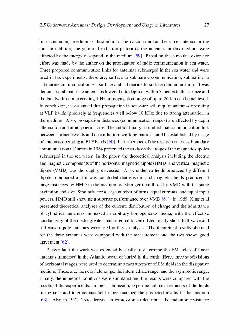
2.1 Antenna operation between the transmitter and the receiver [13] . . . . . 82.2 Hertz experiment of 1887 [17] . . . . . . . . . . . . . . . . . . . . . . . 102.3 Examples of wire antennas . . . . . . . . . . . . . . . . . . . . . . . . . 132.4 Different sizes of horn antennas [22] . . . . . . . . . . . . . . . . . . . . 142.5 Four-element microstrip antenna array operating at 15 GHz band . . . . . 152.6 Nigerian Communication Satellite ground receiving antennas [24] . . . . 162.7 Configurations of lens antennas [13] . . . . . . . . . . . . . . . . . . . . 172.8 Insulated wired antenna on Submarine [37] . . . . . . . . . . . . . . . . 222.9 Antenna inside iron pipe on Submarine [37] . . . . . . . . . . . . . . . . 232.10 Long wire antenna trailing Submarine [37] . . . . . . . . . . . . . . . . . 232.11 Loop antenna fixed on Submarine [38, 39] . . . . . . . . . . . . . . . . . 242.12 Refraction of radio wave at the surface of water [39, 49] . . . . . . . . . 252.13 Polyfoam rafts supporting antennas with electronics systems as developed
and used by the authors [66] . . . . . . . . . . . . . . . . . . . . . . . . 292.14 General overview of Project Sanguine [70] . . . . . . . . . . . . . . . . . 302.15 The proposed project Sanguine by U.S. Navy [39] . . . . . . . . . . . . . 302.16 BCA antennas [71] . . . . . . . . . . . . . . . . . . . . . . . . . . . . . 322.17 Air-Water Interface transmission in fresh water at 1.8 MHz through two
submerged antennas [83] . . . . . . . . . . . . . . . . . . . . . . . . . . 352.18 Communication between submarine and Nevada site [92] . . . . . . . . . 372.19 Standalone transmitting and receiving loop antenna [94] . . . . . . . . . 382.20 HI-Q antenna [95] . . . . . . . . . . . . . . . . . . . . . . . . . . . . . . 392.21 Connectivity between BCAA and submarine through fiber optic [101] . . 412.22 Proposed buoyant cable antenna array [101] . . . . . . . . . . . . . . . . 422.23 Proposed transmitting and receiving wire antennas [106] . . . . . . . . . 432.24 Attenuation measurements in fresh water at VHF band [112] . . . . . . . 482.25 Apparatus for Smith’s experiments [115] . . . . . . . . . . . . . . . . . . 492.26 Side view of Dielectric Resonator antenna [118] . . . . . . . . . . . . . . 502.27 Angle-view of proposed Bow-tie patch antenna [124] . . . . . . . . . . . 512.28 Underwater Small loop antenna in a water container [127] . . . . . . . . 52
3.1 Behavior of σ /ωε as a function of frequency in fresh and sea water [139] 633.2 Attenuation coefficient of an electromagnetic wave propagating in water
with different conductivity . . . . . . . . . . . . . . . . . . . . . . . . . 643.3 Skin depth as a function of frequency for tap, fresh and sea water . . . . . 653.4 Refraction losses as a function of frequency for tap, fresh and sea water . 67
xiii

xiv LIST OF FIGURES
3.5 Intrinsic impedance as a function of conductivity . . . . . . . . . . . . . 683.6 Block diagram for solving antenna radiation [13, 39, 143] . . . . . . . . . 693.7 Geometrical arrangement showing the associated fields of an Hertzian
dipole [8] . . . . . . . . . . . . . . . . . . . . . . . . . . . . . . . . . . 713.8 Antenna’s Field Regions [13, 143] . . . . . . . . . . . . . . . . . . . . . 733.9 Near-Field (reactive near field and radiative near field) and Far-Field of
an antenna[13, 144] . . . . . . . . . . . . . . . . . . . . . . . . . . . . . 75
4.1 Antenna geometry . . . . . . . . . . . . . . . . . . . . . . . . . . . . . . 804.2 Feko model of the antennas . . . . . . . . . . . . . . . . . . . . . . . . . 824.3 Simulations results for change in antenna materials . . . . . . . . . . . . 844.4 Resonance frequency as a function of conductivity . . . . . . . . . . . . 854.5 Input impedance as a function of conductivity . . . . . . . . . . . . . . . 864.6 Resonance frequency as a function of coating thickness . . . . . . . . . . 874.7 Real part input impedance as a function of coating thickness . . . . . . . 874.8 Antenna inside air-filled casing . . . . . . . . . . . . . . . . . . . . . . . 884.9 Resonating frequency and input impedance as a function of casing size . . 894.10 Reflection coefficient as a function frequency for the three antennas in
fresh water . . . . . . . . . . . . . . . . . . . . . . . . . . . . . . . . . 914.11 3D radiation pattern of the antennas in fresh water . . . . . . . . . . . . . 924.12 2D radiation pattern for the three antennas . . . . . . . . . . . . . . . . . 934.13 Reflection coefficient as a function frequency for the three antennas in sea
water . . . . . . . . . . . . . . . . . . . . . . . . . . . . . . . . . . . . 944.14 3D radiation pattern of the antennas in sea water . . . . . . . . . . . . . . 944.15 (a) J-pole (b) Super J-pole (c) Collinear J-pole antennas . . . . . . . . . . 954.16 (a) J-pole (b) Super J-pole (c) Collinear J-pole antennas . . . . . . . . . . 964.17 Reflection coefficient against frequency for the three antennas operating
in freshwater . . . . . . . . . . . . . . . . . . . . . . . . . . . . . . . . 974.18 Modified Reflection coefficient against frequency for the antennas in fresh
water . . . . . . . . . . . . . . . . . . . . . . . . . . . . . . . . . . . . 984.19 Circuits showing capacitors added to cancel inductive load for the antennas 994.20 Reflection coefficient for the J-pole antenna configurations in seawater . 1004.21 Matching circuit for the antennas in sea water . . . . . . . . . . . . . . . 1014.22 Radiation pattern of the antennas in sea water . . . . . . . . . . . . . . . 1024.23 Protractor used in measurement of radiation pattern in freshwater . . . . . 1034.24 Fabricated J-pole and super J-pole antennas . . . . . . . . . . . . . . . . 1044.25 Measurement setup showing the antennas inside the pool . . . . . . . . . 1044.26 Reflection coefficient for the J-pole antenna . . . . . . . . . . . . . . . . 1054.27 Reflection coefficient for the super J-pole antenna . . . . . . . . . . . . . 1064.28 Radiation pattern for the Jpole antenna . . . . . . . . . . . . . . . . . . . 1074.29 Radiation pattern for the super J-pole antenna . . . . . . . . . . . . . . . 1084.30 Prototype of MARES Autonomous Underwater Vehicle [153] . . . . . . 1094.31 Prototype of TriMARES Autonomous Underwater Vehicle [154] . . . . . 1094.32 Model of Autonomous Underwater Vehicle . . . . . . . . . . . . . . . . 1104.33 Antennas placed outside the body of AUV model . . . . . . . . . . . . . 1114.34 Reflection coefficient as a function of frequency for the antennas . . . . . 112
LIST OF FIGURES xv
4.35 Radiation pattern for the antennas with AUV model . . . . . . . . . . . . 113
5.1 Dual band dipole antenna . . . . . . . . . . . . . . . . . . . . . . . . . . 1165.2 Dual band J-pole antenna . . . . . . . . . . . . . . . . . . . . . . . . . . 1165.3 Dual band Dipole and J-pole antenna . . . . . . . . . . . . . . . . . . . . 1175.4 Input impedance as a function of spacing between antenna arms . . . . . 1185.5 Mismatch loss as a function of spacing between antenna arms . . . . . . . 1195.6 Measurement set-up for dual band dipole antenna . . . . . . . . . . . . . 1195.7 Fabricated dual band dipole antenna . . . . . . . . . . . . . . . . . . . . 1205.8 Reflection coefficient against resonance frequency for dual band dipole
antenna . . . . . . . . . . . . . . . . . . . . . . . . . . . . . . . . . . . 1205.9 2D radiation pattern for dual band dipole antenna at 30 MHz . . . . . . . 1215.10 2D radiation pattern for dual band dipole antenna at 60 MHz . . . . . . . 1225.11 Dipole antennas with parasitic elements . . . . . . . . . . . . . . . . . . 1245.12 Reflection coefficient against frequency for the two antennas . . . . . . . 1255.13 Radiation pattern of the antennas in E-plane at 25 MHz . . . . . . . . . . 1255.14 Radiation pattern of the antennas in E-plane at 40 MHz . . . . . . . . . . 1265.15 Radiation pattern of the antennas in H-plane at 25 MHz . . . . . . . . . . 1265.16 Radiation pattern of the antennas in H-plane at 40 MHz . . . . . . . . . . 1275.17 S21 as a function the distance between two antennas for both DipP and DipH1285.18 Photographs of the DipP antenna after fabrication and during measurement 1295.19 Simulation versus measurement for the DipP Antenna . . . . . . . . . . . 1305.20 Simulation versus measurement of the 2-D radiation pattern at 25 MHz . 1315.21 Simulation versus measurement of the 2-D radiation pattern at 40 MHz . 1325.22 The antennas placed horizontally to circular ground planes . . . . . . . . 1335.23 The antennas placed horizontally to square ground planes . . . . . . . . . 1335.24 Reflection coefficient against frequency for the antennas on circular
ground plane . . . . . . . . . . . . . . . . . . . . . . . . . . . . . . . . 1355.25 Reflection coefficient against frequency for the antennas on square ground
plane . . . . . . . . . . . . . . . . . . . . . . . . . . . . . . . . . . . . . 1355.26 Directivity against frequency for the antennas . . . . . . . . . . . . . . . 1365.27 3D radiation pattern of the antenna at 50 MHz, 60 MHz, and 70 MHz
respectively . . . . . . . . . . . . . . . . . . . . . . . . . . . . . . . . . 1365.28 Manufactured square loop antenna with square ground plane . . . . . . . 1375.29 Set up for the measurements . . . . . . . . . . . . . . . . . . . . . . . . 1385.30 Simulation versus Measurement Square Loop Antenna with Reflector . . 1395.31 Radiation pattern of the antenna at 50 MHz (a) E-plane, (b) H-plane . . . 1405.32 Radiation pattern of the antenna at 60 MHz (a) E-plane, (b) H-plane . . . 1415.33 Radiation pattern of the antenna at 70 MHz (a) E-plane, (b) H-plane . . . 1425.34 Prototype of communication unit for ¡VAMOS! project . . . . . . . . . . 1435.35 Isometric view of double helical antenna . . . . . . . . . . . . . . . . . . 1445.36 Antennas inside frame with ground reflector without epoxy . . . . . . . . 1465.37 Antennas covered by epoxy inside frame with ground reflector . . . . . . 1465.38 Reflection coefficient against frequency for the antennas without epoxy . 1475.39 Reflection coefficient against frequency for the antennas with epoxy . . . 1485.40 Radiation pattern of the antennas in E-plane . . . . . . . . . . . . . . . . 148

xvi LIST OF FIGURES
5.41 Radiation pattern of the antennas in H-plane . . . . . . . . . . . . . . . . 1495.42 Fabricated dipole antenna for the project . . . . . . . . . . . . . . . . . . 1495.43 Fabricated loop antenna for the project . . . . . . . . . . . . . . . . . . . 1505.44 Gain against frequency for dipole antenna . . . . . . . . . . . . . . . . . 1535.45 Gain against frequency for dipole antenna with parasitic element . . . . . 1545.46 Gain against frequency for J-pole antenna . . . . . . . . . . . . . . . . . 1555.47 Gain against frequency for collinear J-pole antenna . . . . . . . . . . . . 155
6.1 Two iterations snowflake fractal antenna . . . . . . . . . . . . . . . . . . 159
List of Tables
2.1 ITU’s table of frequency bands [18, 21] . . . . . . . . . . . . . . . . . . 122.2 Comparison between three underwater technologies . . . . . . . . . . . . 202.3 Antennas for underwater communications in sea water . . . . . . . . . . 442.4 Antennas for underwater communications in fresh water . . . . . . . . . 53
3.1 Field Quantities . . . . . . . . . . . . . . . . . . . . . . . . . . . . . . . 553.2 Universal constants . . . . . . . . . . . . . . . . . . . . . . . . . . . . . 553.3 Attenuation values at different frequencies for tap, fresh and sea water . . 653.4 Field regions of half-wave dipole antenna in fresh water . . . . . . . . . . 76
4.1 Typical values of the major water properties @ 25C . . . . . . . . . . . 794.2 Dimension of the antennas . . . . . . . . . . . . . . . . . . . . . . . . . 834.3 Simulation results of the antennas in fresh Water . . . . . . . . . . . . . . 904.4 Simulation Results of the Antennas in sea Water . . . . . . . . . . . . . . 924.5 Dimension of the J-pole antenna configurations in freshwater . . . . . . . 974.6 Simulation results of the antennas in fresh water . . . . . . . . . . . . . . 984.7 Dimension of the J-pole antenna configurations in seawater . . . . . . . . 1004.8 Simulation results of the J-pole antenna configurations in Sea Water . . . 1014.9 MARES main characteristics [153] . . . . . . . . . . . . . . . . . . . . . 1064.10 Simulation Results for the modified Antennas with AUV models . . . . . 110
5.1 Dimension of the Antennas . . . . . . . . . . . . . . . . . . . . . . . . . 1235.2 Dimension of loop antenna with ground reflector . . . . . . . . . . . . . 1305.3 Directivities of the antennas versus operating frequencies . . . . . . . . . 134
xvii

xviii LIST OF TABLES

Abbreviations and Symbols
AUV Autonomous underwater vehiclesBCA Buoyant cable antennaCDMA Code Division Multiple AccessCSA Cavity-backed Slot AntennaDARPA Defence Advanced Research Projects AgencyDRA Dielectric Resonator AntennaEHF Extremely High FrequencyEFL Electric Field LineELF Extremely Low FrequencyEM ElectromagneticFEUP Faculty of Engineering University of PortoGPS Global Positioning SystemsGO Geometrical OpticsGSM Global System for mobile communicationsGTD Geometrical Theory of DiffractionH2020 Horizon 2020HDPE High-density polyethyleneHF High FrequencyHED Horizontal Electric DipoleHMD Horizontal Magnetic DipoleIEEE Institute of Electrical and Electronics EngineersINESCTEC Institute for Systems and Computer Engineering, Technology and ScienceIOT Internet of ThingsISI Inter Symbol InterferenceLEO Low Earth OrbitLF Low FrequencyLORAN-C long range navigation-CLOS line-of-sightLTE Long term EvolutionMF Medium FrequencyMFL Magnetic Field LoopMMIC Monolithic Microwaves Integrated CircuitOC Optical CommunicationPEC Perfect Electric ConductorPCS Personal Communication Service
xix
xx ABBREVIATIONS AND SYMBOLS
RADAR Radio Detection and RangingRF Radio FrequencyRFID Radio Frequency IdentificationROV Remotely Operated VehiclesRR Radio RegulationsSEAFARER Surface ELF Antenna For Addressing REmotely-deployed ReceiversSI International StandardSINR Signal to Interference plus Noise RatioSLF Super Low FrequencySNR Signal to noise ratioSQUID Superconducting Quantum Interference DeviceSHF Super High FrequencyTHF Terahertz High FrequencyTWA Traveling Wave AntennaUHF Ultra High FrequencyULF Ultra Low FrequencyUMTS Universal Mobile Telecommunications SystemURFC Underwater Radio Frequency CommunicationUTD Uniform Theory of DiffractionUWB UltrawidebandVAMOS Viable Alternative Mine Operating SystemVED Vertical Electric DipoleVEIN velocity induced electrode noiseVHF Very High FrequencyVLF Very Low FrequencyVMD Vertical Magnetic DipoleWI-FI Wireless FidelityWiMAX Worldwide Interoperability for Microwave AccessWLAN Wireless Local Area NetworkWRC World radiocommunication ConferenceWWW World Wide Web
Chapter 1
Introduction
Transmission and reception of signals in aqueous environments require intense studyand understanding of various parameters that can cause impairments or degradationthereby altering the propagation phenomenon of signals and devices immersed in it.There has also been an increasing demand for high-speed wireless communicationlinks for underwater applications, which include: oceanographic data collection whichwill require data exchange between two or more Autonomous Underwater Vehicles(AUVs) and other underwater sensors, coastline protection and surveillance, underwaterenvironmental observation for exploration and off-shore oil and gas field monitoring. Inthese applications, communications require downloading of mission data from the AUV tothe docking station, successful docking of the AUV at the station for recharging throughwireless power transfer [1], exchange of data between AUVs and underwater wirelesssensor nodes.
In underwater communication there are three established technologies through whichunderwater communications have been considered, they are; acoustics and ultrasonicsignals, optical signals, and radio frequency (RF) signal [2]. Due to the variousadvantages of the technologies, each of these is most appropriate for different underwaterapplications. For instance, when long-range propagation (up to tens of kilometers) infresh or sea water is of paramount concern, as seen in the case of submarines, whichare submerged in hundreds of meters below the water surface and communicating witha location on the earth surface, acoustic and ultrasonic systems are the most appropriatetechnology [3, 4, 5]. Similarly, when the distance is considerably long and high data-rateswith low latency is expected, optical communication systems remain the best technology[4, 5, 6]. On the other hand, for a short-range and relatively high-speed communication,which is important for real-time voice, video and data exchange, EM signals will ensuresmooth communication in this regards [2]. Despite these advantages, each of the
1
2 Introduction
technologies still has its disadvantages. The acoustic and ultrasonic signal is unfit forreal-time and broadband underwater wireless sensor networks because of poor immunityto noise, low data-rates, and high channel latency. In like manner, optical communicationrequires very good alignment and are as well affected by suspended particles in water andmarine fouling. The major disadvantage of EM signals is attenuation, which imposeslimits on its usage for underwater communications, as it increases with increasingoperating frequency [7, 8]. Thus, the main concern of this thesis is to present the design,simulation, construction and measurements of underwater antennas, which will be utmostuseful in various underwater applications by scuba divers, oceanographers, underwaterphotographers, and underwater miners. The performance of these antennas is accessedin fresh water for maximum directivity which is important for propagation distance andbandwidths for the data rates at this distance.
1.1 Motivation
The motivation for this work is to improve short-range communications which mayexist between transmitting/receiving devices on scuba divers on one hand and withunderwater elements (AUV, ROV (Remotely Operated Vehicles), sensor nodes) on theother hand or between an AUV and docking station, through the usage of underwaterradio frequency communications. Robotic based activities in the underwater environmentrequired sufficient bandwidth, improved propagation distance, and minimal attenuation,for real-time transmission and reception of signals in the medium. Hence, whatmeasure(s) can be taken to ensure that the system suffers minimal attenuation? How alsocan propagation distance be improved for the underwater antennas in the environment?Also, to provide a better alternative to the usage of acoustic communication in theunderwater scenario and for the possibility of combining this technology with eitheracoustic or optical communications in a hybrid underwater network for improvedlong-range communications in deep water scenario.
1.2 Aims and Objectives
To improve communications between underwater users and equipment throughunderwater radio frequency communications (URFC), the objective of this work is thedesign of antennas for underwater communications, followed by fabrication of theseantennas, test and measurement.
1.3 Thesis Organization 3
1.2.1 Objectives
• To develop portable underwater antennas suitable for installation on AUV foronward communication with underwater sensor nodes and docking station;
• To develop underwater antennas useful for scuba divers for data harvesting in theshallow water scenario;
• To develop an analytical method that can be used to determine the gain of theseantennas, which will assist in analyzing their performance in a lossy medium;
• To validate these analytical methods through practical measurements of theunderwater antennas;
1.3 Thesis Organization
Beside this introductory chapter, four other chapters and the concluding remarks wereadded thereafter.
Chapter 2 addresses the review of underwater antennas with respect to designs,developments, and usage. This chapter comprises:
• definitions of antennas, brief history, and types.
• Underwater technologies with a table showing similarities and differences of thetechnologies;
• Extensive review of the state of the art with respect to antenna design and EMpropagation in underwater environments, spanning around a century.
In chapter 3, the propagation of electromagnetic waves in lossless and lossy mediais presented. This includes theoretical information regarding propagation in water,determination of the radiation characteristics of antennas submerged in lossy mediumand also factors that affect RF propagation in the medium.
In chapter 4, full analyses of underwater antennas regarding the effect of the changein materials of the wire, the coating of the wire of the designed antennas, change inconductivity of the medium and when the antennas are placed in an air-filled casing werepresented. In the second part, the performance of designed narrow band antennas wasalso presented.
In chapter 5, the performance of antennas with dual and wideband capabilities areassessed with respect to their radiation characteristics and bandwidth. Also presented in

4 Introduction
this chapter are the antennas designed in a European project that our team partnered with.Though these antennas were originally designed as wideband, in order to ensure that theantennas were secured against water waves in the medium, addition of materials withdifferent permittivities and their final performance is further investigated. Final in thischapter, realized gain and link budget of underwater antennas is presented.
Chapter 6 is the final chapter of this thesis, where final conclusion is drawn and thefuture works were also presented.
1.4 Contributions
The main contributions of this research are summarized below
• Model approach to the usage of wire antennas for narrow, dual and widebandcommunication in the underwater environment;
• Designing of underwater antennas at a specified resonating frequency;
• Modeling of directional underwater antennas for improved propagation distance;
• Underwater antenna modeling around the body of Autonomous Underwatervehicles;
• Experimental measurements of the radiation pattern of underwater antennas;
• Determination of realized gains of underwater antennas;
1.5 Publications
The following publications are the results of these contributions:
1. S. I. Inacio, M. R. Pereira, H. M. Santos, L. M. Pessoa, F. B. Teixeira, M. J.Lopes, O. Aboderin and H. M. Salgado, "Antenna design for underwater radiocommunications" OCEANS, Shanghai China, 2016;
2. S. I. Inacio, M. R. Pereira, H. M. Santos, L. M. Pessoa, F. B. Teixeira, M. J.Lopes, O. Aboderin and H. M. Salgado, "Dipole Antenna for Underwater RadioCommunication" Underwater Communications Network (UComms), Lerici Italy,2016;
3. L. M. Pessoa, M. R. Pereira, O. Aboderin, H. M. Salgado, and S. I. Inácio, “Antennafor underwater radio communications,” patent ep 3 291 364A1;

1.5 Publications 5
4. O. Aboderin, S. I. Inacio, H. M. Santos, M. R. Pereira, L. M. Pessoa andH. M. Salgado, "Analysis of J-Pole Antenna Configurations for UnderwaterCommunications" OCEAN, Monterey California, United States of America, 2016;
5. O. Aboderin and L. M. Pessoa and H. M. Salgado, "Performance evaluation ofantennas for underwater applications" Wireless Days 2017, Porto Portugal;
6. O. Aboderin, L. M. Pessoa and H. M. Salgado, "Analysis of loop antennawith ground plane for underwater communications," OCEANS 2017 - Aberdeen,Aberdeen, 2017;
7. O. Aboderin, L. M. Pessoa and H. M. Salgado, "Wideband dipole antennas withparasitic elements for underwater communications" OCEANS 2017 - Aberdeen,Aberdeen, 2017;
8. O. Aboderin and L. M. Pessoa and H. M. Salgado, "Analysis of Antennas Designedfor Fresh Water Applications" to be submitted to IEEE Access;
9. O. Aboderin and L. M. Pessoa and H. M. Salgado, "A Survey of UnderwaterAntennas: Designs, Developments and Applications" To be submitted to IEEECommunications Surveys & Tutorials.

6 Introduction
Chapter 2
Review of Underwater Antennas:Designs, Developments and Usage
2.1 Introduction
The much breakthrough in modern-day scientific research and technology can beattributed to the military exploits mostly around the first and second world wars. Someof the technologies that benefited from military activities include the antenna designsand development, satellite communication, Internet network, underwater communicationsamong others [9]. Antenna, therefore, has proven to be an integral part of othertechnologies as the reliant on its usage cuts across different applications in spacescience, terrestrial networks, and underwater communications. In space science, antennaremains one of the most important equipment that ensures respective transmission andreception of telecommand and telemetry data, to and from satellites launched into orbitsthat is thousands of kilometers away from the earth’s surface. Similarly, terrestrialnetworks has witnessed evolution from; wired to wireless, copper wire to fiber opticwhere long-distance transmission and interference which are limited to the former arewell resolved in the latter, analog to digital, which include metamorphosing from firstgeneration (1G) to the most recent fifth generation (5G) networks, whilst still lookingahead to the sixth generation (6G) [10, 11]. The need for high-speed, short-rangecommunication for relevant applications in the context of underwater exploration andmining makes the development of various antennas that are capable of meeting theserequirements of great importance to scuba divers, underwater miners, and other users.Therefore, this chapter begins discussing antenna as a whole with respect to its definition,history and types. Also, major technologies that ensure smooth communications in theunderwater environment are compared and extensive review of designing, developing and
7
8 Review of Underwater Antennas: Designs, Developments and Usage
usage of underwater antennas over many decades and for many services is finally given.
2.2 Antenna in Communication Systems
One of the most critical components importantly needed in the communication systems(mobile, wired and wireless) in any medium is an antenna. The increasing need ofimproving communication mechanism; in household equipment (including televisionantennas (loop or Yagi), multi-functional cell phones, hand-held portable devices,long-range communications, electronic chips (including Radio Frequency Identification(RFIDs)) and most recently Internet of Things (IoT) has made the entire globe to dependon antennas for day-to-day activities. In actual fact, antennas in their millions are soubiquitous worldwide.
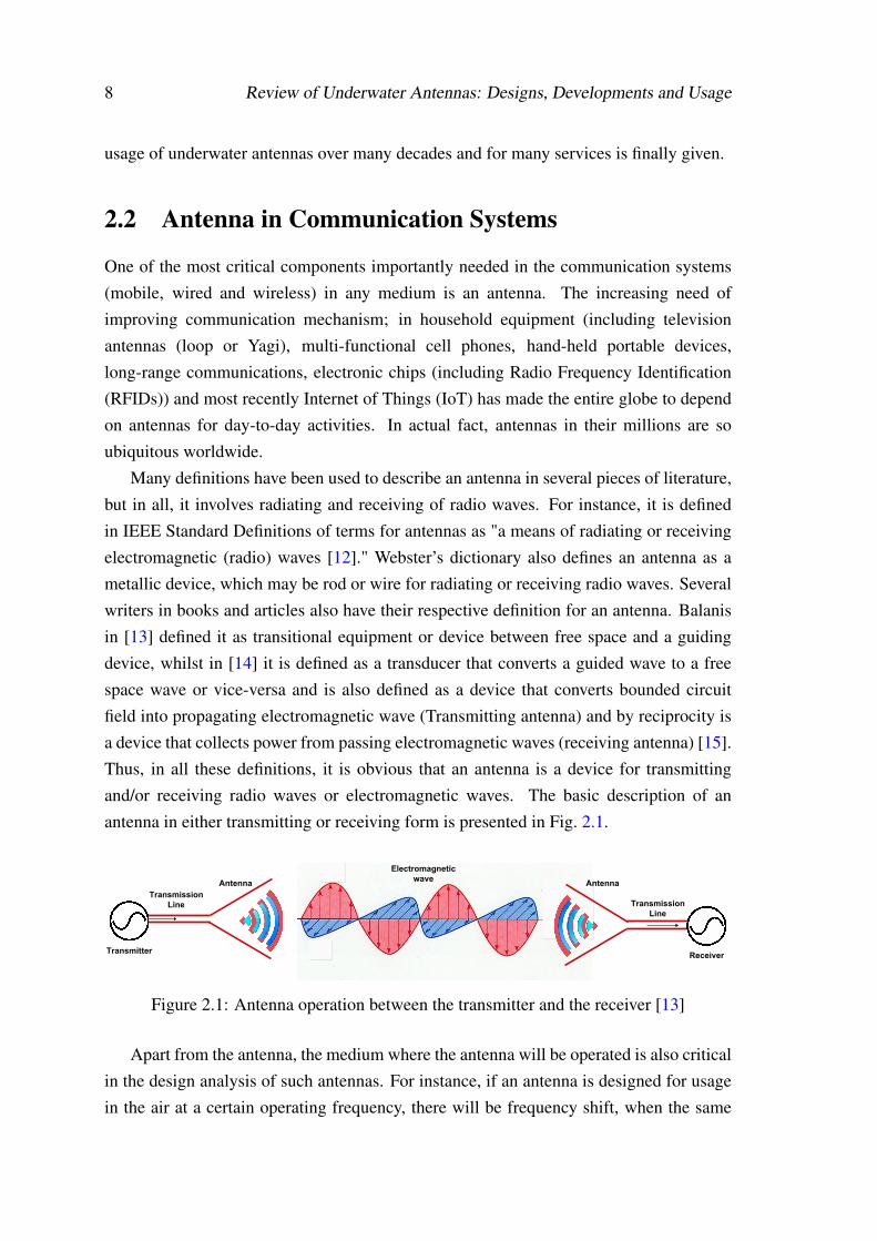
Many definitions have been used to describe an antenna in several pieces of literature,but in all, it involves radiating and receiving of radio waves. For instance, it is definedin IEEE Standard Definitions of terms for antennas as "a means of radiating or receivingelectromagnetic (radio) waves [12]." Webster’s dictionary also defines an antenna as ametallic device, which may be rod or wire for radiating or receiving radio waves. Severalwriters in books and articles also have their respective definition for an antenna. Balanisin [13] defined it as transitional equipment or device between free space and a guidingdevice, whilst in [14] it is defined as a transducer that converts a guided wave to a freespace wave or vice-versa and is also defined as a device that converts bounded circuitfield into propagating electromagnetic wave (Transmitting antenna) and by reciprocity isa device that collects power from passing electromagnetic waves (receiving antenna) [15].Thus, in all these definitions, it is obvious that an antenna is a device for transmittingand/or receiving radio waves or electromagnetic waves. The basic description of anantenna in either transmitting or receiving form is presented in Fig. 2.1.
Electromagnetic waveAntenna
Transmitter
Transmission Line
Antenna
Receiver
Transmission Line
Figure 2.1: Antenna operation between the transmitter and the receiver [13]
Apart from the antenna, the medium where the antenna will be operated is also criticalin the design analysis of such antennas. For instance, if an antenna is designed for usagein the air at a certain operating frequency, there will be frequency shift, when the same
2.2 Antenna in Communication Systems 9
antenna is encased in a glass or plastic box, due to change in its surrounding medium.There will be further shifting in the operating frequency when the antenna is immersedin water, which is also depending on whether it is fresh or sea water. All these frequencyshifts depend on change in the permittivity and conductivity of the surrounding mediumof the antenna.
2.2.1 Brief History of Antennas
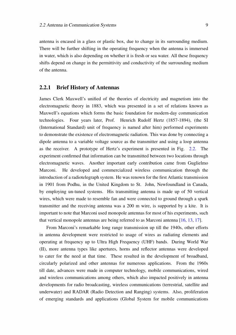
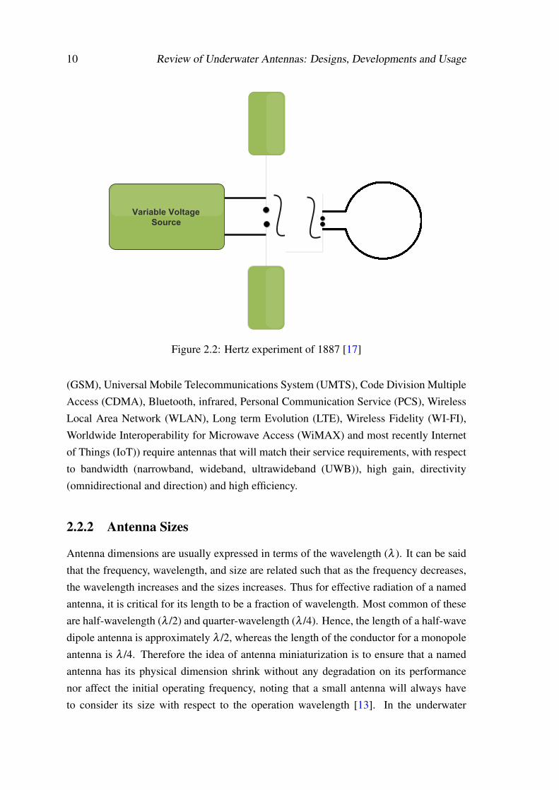
James Clerk Maxwell’s unified of the theories of electricity and magnetism into theelectromagnetic theory in 1883, which was presented in a set of relations known asMaxwell’s equations which forms the basic foundation for modern-day communicationtechnologies. Four years later, Prof. Henrich Rudolf Hertz (1857-1894), (the SI(International Standard) unit of frequency is named after him) performed experimentsto demonstrate the existence of electromagnetic radiation. This was done by connecting adipole antenna to a variable voltage source as the transmitter and using a loop antennaas the receiver. A prototype of Hertz’s experiment is presented in Fig. 2.2. Theexperiment confirmed that information can be transmitted between two locations throughelectromagnetic waves. Another important early contribution came from GuglielmoMarconi. He developed and commercialized wireless communication through theintroduction of a radiotelegraph system. He was renown for the first Atlantic transmissionin 1901 from Podhu, in the United Kingdom to St. John, Newfoundland in Canada,by employing un-tuned systems. His transmitting antenna is made up of 50 verticalwires, which were made to resemble fan and were connected to ground through a sparktransmitter and the receiving antenna was a 200 m wire, is supported by a kite. It isimportant to note that Marconi used monopole antennas for most of his experiments, suchthat vertical monopole antennas are being referred to as Marconi antenna [16, 13, 17].
From Marconi’s remarkable long range transmission up till the 1940s, other effortsin antenna development were restricted to usage of wires as radiating elements andoperating at frequency up to Ultra High Frequency (UHF) bands. During World War(II), more antenna types like apertures, horns and reflector antennas were developedto cater for the need at that time. These resulted in the development of broadband,circularly polarized and other antennas for numerous applications. From the 1960still date, advances were made in computer technology, mobile communications, wiredand wireless communications among others, which also impacted positively in antennadevelopments for radio broadcasting, wireless communications (terrestrial, satellite andunderwater) and RADAR (Radio Detection and Ranging) systems. Also, proliferationof emerging standards and applications (Global System for mobile communications
10 Review of Underwater Antennas: Designs, Developments and Usage
Variable Voltage Source
Figure 2.2: Hertz experiment of 1887 [17]
(GSM), Universal Mobile Telecommunications System (UMTS), Code Division MultipleAccess (CDMA), Bluetooth, infrared, Personal Communication Service (PCS), WirelessLocal Area Network (WLAN), Long term Evolution (LTE), Wireless Fidelity (WI-FI),Worldwide Interoperability for Microwave Access (WiMAX) and most recently Internetof Things (IoT)) require antennas that will match their service requirements, with respectto bandwidth (narrowband, wideband, ultrawideband (UWB)), high gain, directivity(omnidirectional and direction) and high efficiency.
2.2.2 Antenna Sizes
Antenna dimensions are usually expressed in terms of the wavelength (λ ). It can be saidthat the frequency, wavelength, and size are related such that as the frequency decreases,the wavelength increases and the sizes increases. Thus for effective radiation of a namedantenna, it is critical for its length to be a fraction of wavelength. Most common of theseare half-wavelength (λ /2) and quarter-wavelength (λ /4). Hence, the length of a half-wavedipole antenna is approximately λ /2, whereas the length of the conductor for a monopoleantenna is λ /4. Therefore the idea of antenna miniaturization is to ensure that a namedantenna has its physical dimension shrink without any degradation on its performancenor affect the initial operating frequency, noting that a small antenna will always haveto consider its size with respect to the operation wavelength [13]. In the underwater
2.3 Types of Antennas 11
environment, it is important to design an antenna that operates in the frequency bandwhere attenuation effect is minimal, which should be below 400 MHz, as discussed laterin section 3.3. Though it is expected that such an antenna might have a large physicaldimension given the operation frequency (λ = v
f in air) and the wavelength in free spaceequals 0.75 m. But in the underwater environment, the wavelength changes, which is dueto the effect of permittivity (water relative permittivity is 81) and conductivity (0.005 S/min fresh water and 4 S/m in sea water) in this medium and subsequently the dimension ofthe antenna. For instance, if a dipole antenna is designed to operate at 300 MHz; in theair, the wavelength is 1 m, whereas, at the same frequency, the wavelength is 0.124 m and0.077m in fresh and sea water respectively.
2.2.3 Frequency Bands
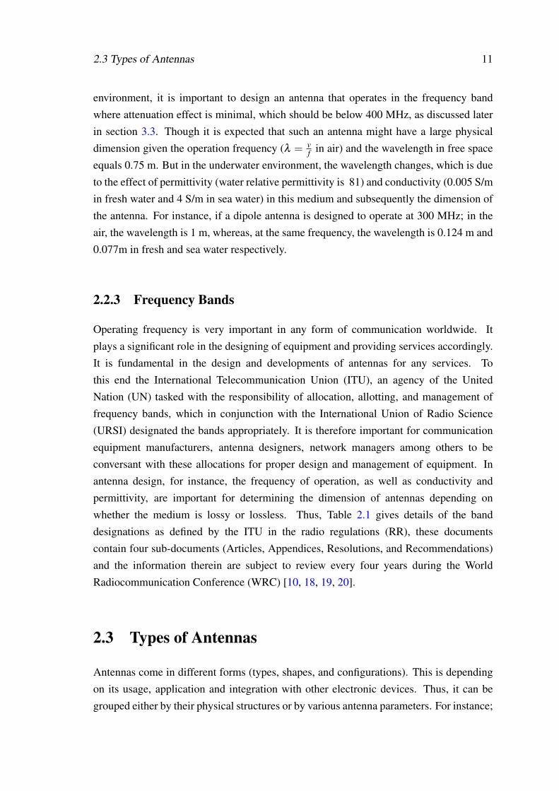
Operating frequency is very important in any form of communication worldwide. Itplays a significant role in the designing of equipment and providing services accordingly.It is fundamental in the design and developments of antennas for any services. Tothis end the International Telecommunication Union (ITU), an agency of the UnitedNation (UN) tasked with the responsibility of allocation, allotting, and management offrequency bands, which in conjunction with the International Union of Radio Science(URSI) designated the bands appropriately. It is therefore important for communicationequipment manufacturers, antenna designers, network managers among others to beconversant with these allocations for proper design and management of equipment. Inantenna design, for instance, the frequency of operation, as well as conductivity andpermittivity, are important for determining the dimension of antennas depending onwhether the medium is lossy or lossless. Thus, Table 2.1 gives details of the banddesignations as defined by the ITU in the radio regulations (RR), these documentscontain four sub-documents (Articles, Appendices, Resolutions, and Recommendations)and the information therein are subject to review every four years during the WorldRadiocommunication Conference (WRC) [10, 18, 19, 20].
2.3 Types of Antennas
Antennas come in different forms (types, shapes, and configurations). This is dependingon its usage, application and integration with other electronic devices. Thus, it can begrouped either by their physical structures or by various antenna parameters. For instance;
12 Review of Underwater Antennas: Designs, Developments and Usage
Table 2.1: ITU’s table of frequency bands [18, 21]
BandNumber Band Name Symbols Frequency
rangeMetricsubdivision
1Extremely LowFrequency ELF 3 - 30 Hz
2Super LowFrequency SLF 30 - 300 Hz
3Ultra LowFrequency ULF 300 - 3000 Hz
4Very LowFrequency VLF 3 - 30 kHz
Myriametricwaves
5LowFrequency LF 30 -300 kHz
Kilometricwaves
6MediumFrequency MF 300 -3000 kHz
Hectometricwaves
7HighFrequency HF 3 - 30 MHz
Decametricwaves
8Very HighFrequency VHF 30 - 300 MHz
Metricwaves
9Ultra HighFrequency UHF 300 - 3000 MHz
Decimetricwaves
10Super HighFrequency SHF 3 - 30 GHz
Centimetricwaves
11Extremely HighFrequency EHF 30 - 300 GHz
Millimetricwaves
12Terahertz HighFrequency THF 300 - 3000 GHz
Decimillimetricwaves
• if grouped with respect to bandwidth, they can be either narrowband or broadband(wideband, ultra-wideband (UWB));
• if organized with respect to their polarization, they can be circular, linearly(horizontal and vertical) or elliptically polarized;
• if divided with respect to their resonance, they can be traveling wave or resonantantennas;
• if classified with respect to the number of elements, they can be element antennasor antenna arrays.
Hence, physical structures have been used to classified antennas into 6 different groups.
2.3 Types of Antennas 13
2.3.1 Wire Antennas
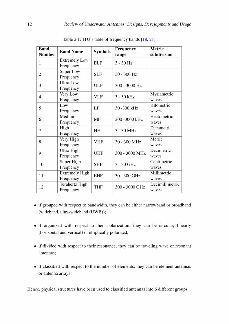
Wire antennas are ubiquitous and seem to be more common than other antenna typesand it is very familiar to a layman as they can be seen virtually everywhere. Theyare low cost, easy to construct and made from conducting wires. These antennasare used in automobiles, personal communications/applications, spacecraft, ships, andbuildings. Various shapes of these antenna types include; Dipole, loop, Helix, J-pole,and spiral. Each of these may take different shapes, through which their performancecan be optimized [17, 13]. Example of wire antennas are presented in Fig. 2.3. Theseantennas have been explored in the context of this thesis for underwater applications andare discussed in chapter 4. It is important to note that wire antennas are more suitableto use in the underwater environment, as it can go directly into the medium, without theneed protect the antennas from water, unlike printed antennas that will require sprayingof Epoxy resin on its either side, which will, therefore, alter the design frequency.
(a) Loop antenna (b) Dipole antenna(c) J-poleantenna
Figure 2.3: Examples of wire antennas
2.3.2 Aperture Antennas
These are antenna types with a physical opening that allows transmission and receptionof electromagnetic waves. Aperture antennas can be flush-mounted, which made themsuitable for use in spacecraft and aircraft. Example of antennas in this category includes;
14 Review of Underwater Antennas: Designs, Developments and Usage
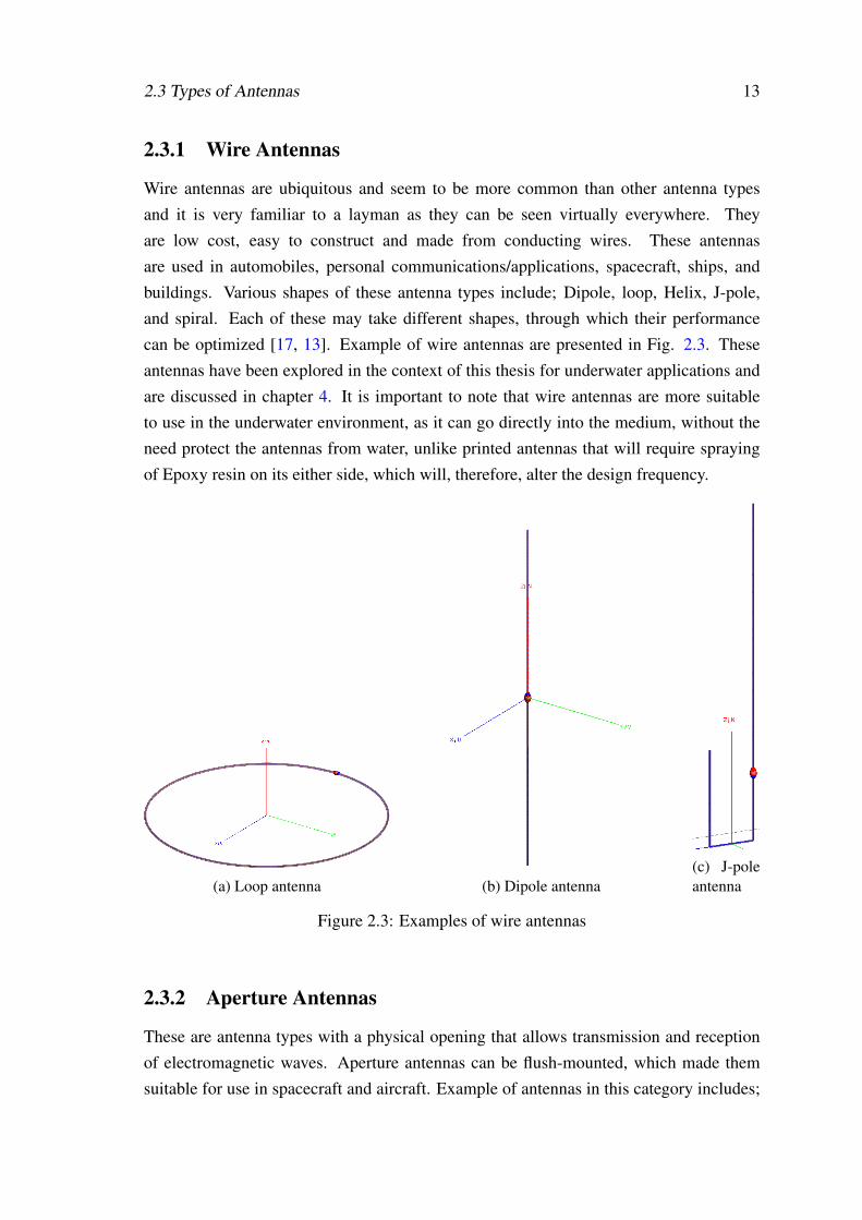
horn antenna, a slot antenna, inverted-F antenna, and slotted waveguide antenna. Hornsantennas are presented in Fig.2.4 comprises of pyramidal (rectangular) and conical(circular) shapes.
Figure 2.4: Different sizes of horn antennas [22]
2.3.3 Microstrip Antennas
Microstrip antennas consist of a metallic patch which can come in different shapes(circular, square, triangular), the substrate and the metallic ground plane. They arebasically conformable to planar and non planar surfaces, low profile, simple or easy todesign, low cost, when mounted on rigid surface they are mechanically robust, compatiblewith Monolithic Microwaves Integrated Circuit (MMIC) and as well very versatile withrespect to their polarization, pattern, resonant frequency and impedance.
2.3.4 Antenna Arrays
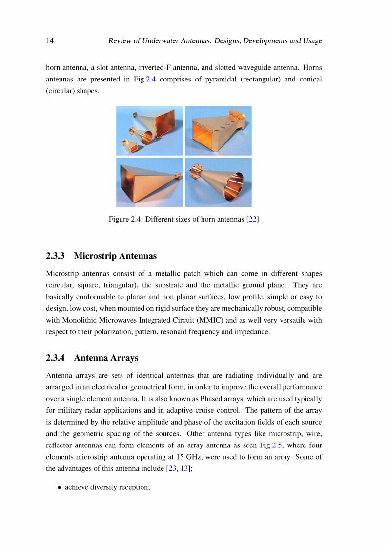
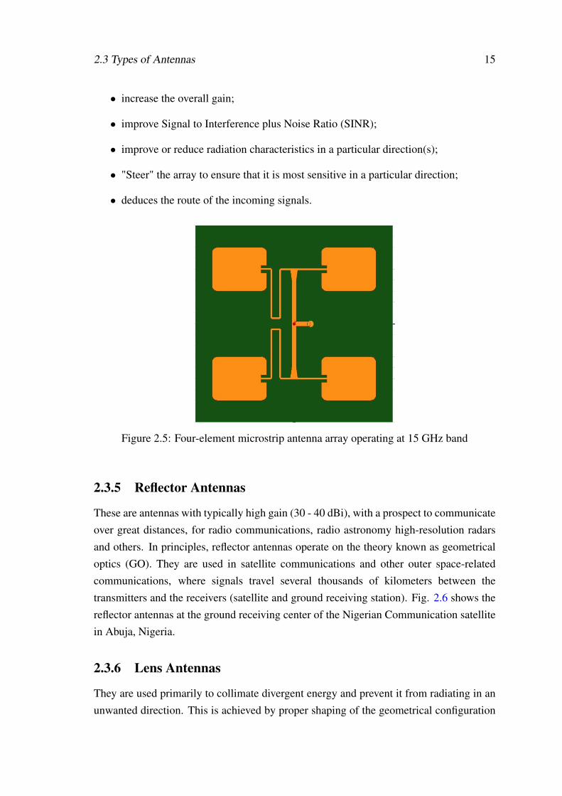
Antenna arrays are sets of identical antennas that are radiating individually and arearranged in an electrical or geometrical form, in order to improve the overall performanceover a single element antenna. It is also known as Phased arrays, which are used typicallyfor military radar applications and in adaptive cruise control. The pattern of the arrayis determined by the relative amplitude and phase of the excitation fields of each sourceand the geometric spacing of the sources. Other antenna types like microstrip, wire,reflector antennas can form elements of an array antenna as seen Fig.2.5, where fourelements microstrip antenna operating at 15 GHz, were used to form an array. Some ofthe advantages of this antenna include [23, 13];
• achieve diversity reception;
2.3 Types of Antennas 15
• increase the overall gain;
• improve Signal to Interference plus Noise Ratio (SINR);
• improve or reduce radiation characteristics in a particular direction(s);
• "Steer" the array to ensure that it is most sensitive in a particular direction;
• deduces the route of the incoming signals.
Figure 2.5: Four-element microstrip antenna array operating at 15 GHz band
2.3.5 Reflector Antennas
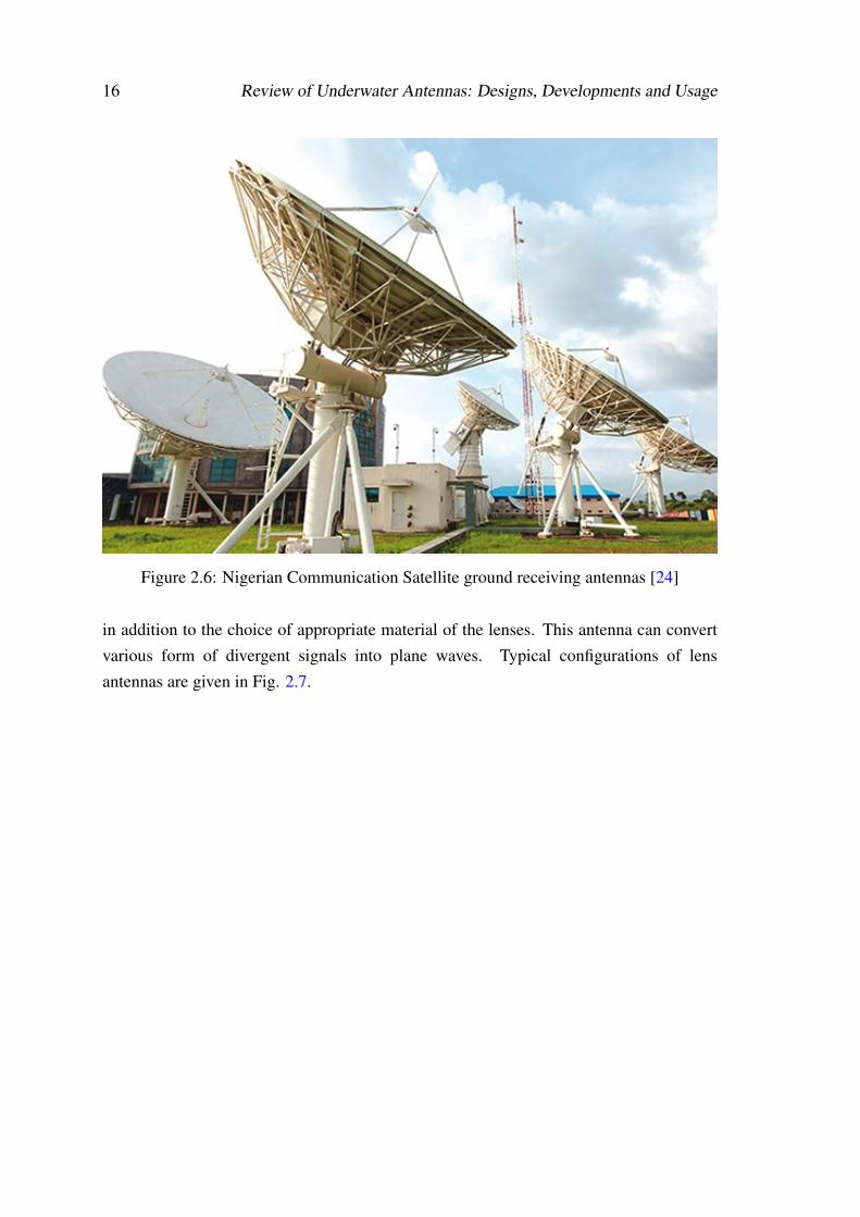
These are antennas with typically high gain (30 - 40 dBi), with a prospect to communicateover great distances, for radio communications, radio astronomy high-resolution radarsand others. In principles, reflector antennas operate on the theory known as geometricaloptics (GO). They are used in satellite communications and other outer space-relatedcommunications, where signals travel several thousands of kilometers between thetransmitters and the receivers (satellite and ground receiving station). Fig. 2.6 shows thereflector antennas at the ground receiving center of the Nigerian Communication satellitein Abuja, Nigeria.
2.3.6 Lens Antennas
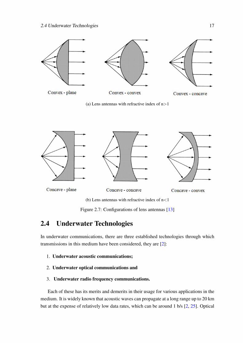
They are used primarily to collimate divergent energy and prevent it from radiating in anunwanted direction. This is achieved by proper shaping of the geometrical configuration
16 Review of Underwater Antennas: Designs, Developments and Usage
Figure 2.6: Nigerian Communication Satellite ground receiving antennas [24]
in addition to the choice of appropriate material of the lenses. This antenna can convertvarious form of divergent signals into plane waves. Typical configurations of lensantennas are given in Fig. 2.7.
2.4 Underwater Technologies 17
(a) Lens antennas with refractive index of n>1
(b) Lens antennas with refractive index of n<1
Figure 2.7: Configurations of lens antennas [13]
2.4 Underwater Technologies
In underwater communications, there are three established technologies through whichtransmissions in this medium have been considered, they are [2]:
1. Underwater acoustic communications;
2. Underwater optical communications and
3. Underwater radio frequency communications.
Each of these has its merits and demerits in their usage for various applications in themedium. It is widely known that acoustic waves can propagate at a long range up to 20 kmbut at the expense of relatively low data rates, which can be around 1 b/s [2, 25]. Optical
18 Review of Underwater Antennas: Designs, Developments and Usage
communications, on the other hand, provide high data rates up to 1 Gbps, at seeminglypropagation distance of about 100 m. On the other hand, wireless propagation of, theradio waves can achieve up to 1 km range with 100 b/s, but the data rates continue todecrease as the propagation distance increases. These three technologies are examinedextensively and are presented as follows.
2.4.1 Underwater Acoustic Communications
Acoustic waves technology has been widely embraced worldwide as a viable solutionfor underwater communication because of its ability to establish long-distance links (upto tens of kilometers). Also, it is characterized by having low attenuation and can evenoperate in the absence of line-of-sight (LOS) between the terminals and in deep water[26, 27]. Despite these advantages, there are many disadvantages such as low datarates (propagates up to 20 Km at almost 1 b/s), high channel round trip delay (channellatency), poor immunity to noise and a high cost of nodes that have led to continuousresearch in alternative technologies. They are also not robust since they are easilyaffected by temperature, ambient noise, turbidity, and pressure gradients. Furthermore,they are dangerous to marine life and the ecosystem. Also, they offer poor propagationin shallow water due to interference [28]. The acoustic signals can also experienceInter-Symbol Interference (ISI), due to the multipath propagation effect [28]. In addition,this technology has low propagation velocity, when compared with other technologies,consequently, it suffers greatly from Doppler effects [29]. Thus, acoustic receivers oftenemploy adaptive equalization [28, 30]. The ambient noise in acoustic communicationsis frequency dependent, which can be traced to a number of sources. For instance, atfrequencies below 100 Hz, the noise is mainly due to marine traffic, whereas wind andrain are significantly responsible for noise at higher frequencies around 100 kHz, the noiselevel is dependent on the intensity of rain and wind. At frequencies beyond this, thermalnoise, whose spectral density increases with frequency, is involved [28]. Despite thesedisadvantages, the technology is still being used around the world but other technologiesare also gaining acceptance because of their advantages over acoustic systems.
2.4.2 Underwater Optical Communications
Apart from acoustic communications, another technology that has been widely used inthe underwater environment is Optical Communication (OC). OC is as an alternativetechnology that provides ultra-high data rates up to the Gigabit per second (Gbps) andabout 10-150 Mbps over moderate propagation distances (10-100 meters) [31]. It is
2.4 Underwater Technologies 19
also immune to transmission round-trip delay, which is an advantage over acousticcommunications. Likewise, it offers guaranteed signal fidelity (secured link) and lowpower consumption, among other things. However, this technology can only be used forshort-range communications because of the strong backscatter from suspended particlesand severe water absorption at the optical frequency band [32]. It also requires goodalignment or line of sight for its propagation. Apart from these, optical waves are difficultto use for cross communications from seawater to air and vice versa, and they are alsoaffected by scattering and absorption. They can also propagate at moderate link range (upto tens of meters) [31].
2.4.3 Underwater Radio Frequency Communications
The third technology, which can also be used for underwater communications is basedon Electromagnetic (EM) waves in the radio frequency (RF) range. Usage of RF inthe underwater environment began as a dream in the middle of the twentieth century,but further experiments have shown that when RF signal is coupled with digital signalcompression, it has greater advantages than other technologies in the underwater scenario[25]. Apart from these, radio signals allow flexibility in the deployment of a wirelesssensor network for coastal monitoring applications. This is nearly impossible with othertechnologies because of the high level of aeration and sediments present in coastal water.In water, EM waves propagate at a velocity that is about 4 times faster than that ofthe acoustic waves. This implies that Doppler shift and propagation delay or latencyare significantly reduced and subsequently this technology is suitable for real-time datatransfer [3, 26, 4, 5, 33].
Besides, it has also been proven that RF waves are less sensitive to reflection andrefraction in shallow waters than the acoustic waves. This helps in reducing the multipatheffect. In addition, the nature of water (dirty or clean) and suspended particles havevery little or no impact on the RF waves. Also, it has no known effects on marinelives [34]. Furthermore, using the same technology, AUVs and ROVs can be chargedat underwater docking station through wireless power transfer [1]. In terms of alignment,RF waves do not require strong alignment or LOS for propagating in any medium andare immune to acoustic noise. It also has the capability for cross-boundary transmission,that is water-to-air transmission or vice versa. This ensures long-range communicationfor the RF wave. In addition, out of the aforementioned technologies, it is the leastaffected by tidal waves or water turbulence [35, 25]. Moreover, RF waves do not requiremechanical tunning, which is required with the acoustic communications and neither doesit require surface repeaters especially when interfacing the water-air boundary [25, 6].
20 Review of Underwater Antennas: Designs, Developments and Usage
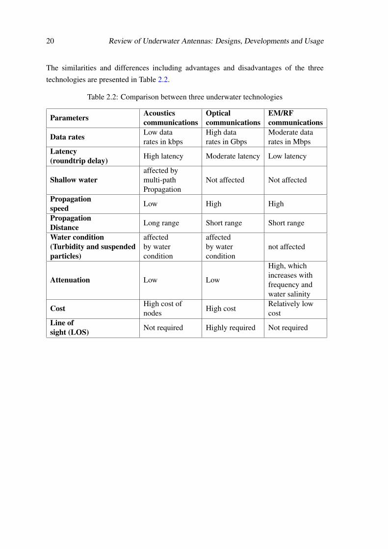
The similarities and differences including advantages and disadvantages of the threetechnologies are presented in Table 2.2.
Table 2.2: Comparison between three underwater technologies
Parameters Acousticscommunications
Opticalcommunications
EM/RFcommunications
Data rates Low datarates in kbps
High datarates in Gbps
Moderate datarates in Mbps
Latency(roundtrip delay) High latency Moderate latency Low latency
Shallow wateraffected bymulti-pathPropagation
Not affected Not affected
Propagationspeed Low High High
PropagationDistance Long range Short range Short range
Water condition(Turbidity and suspendedparticles)
affectedby watercondition
affectedby watercondition
not affected
Attenuation Low Low
High, whichincreases withfrequency andwater salinity
Cost High cost ofnodes High cost
Relatively lowcost
Line ofsight (LOS) Not required Highly required Not required
2.5 Underwater Antennas: Design, Development and Usage in Literatures 21
2.5 Underwater Antennas: Design, Development andUsage in Literatures
Antenna developments for underwater applications have been in the literature for morethan a century. These developments have been considered in fresh and sea waters, withrespect to the operations and usages in each medium. To this end, antenna design,developments and usage in sea water and fresh water are as presented in the subsections.
2.5.1 Antenna Developments for Usage in Sea Water
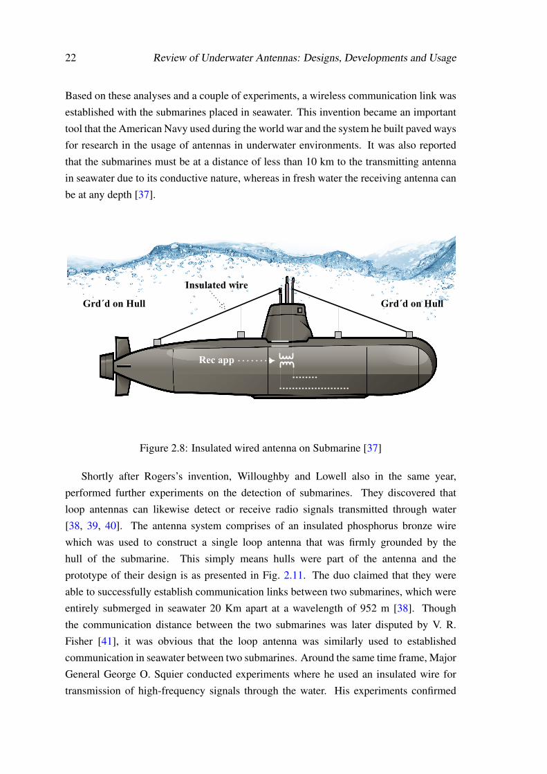
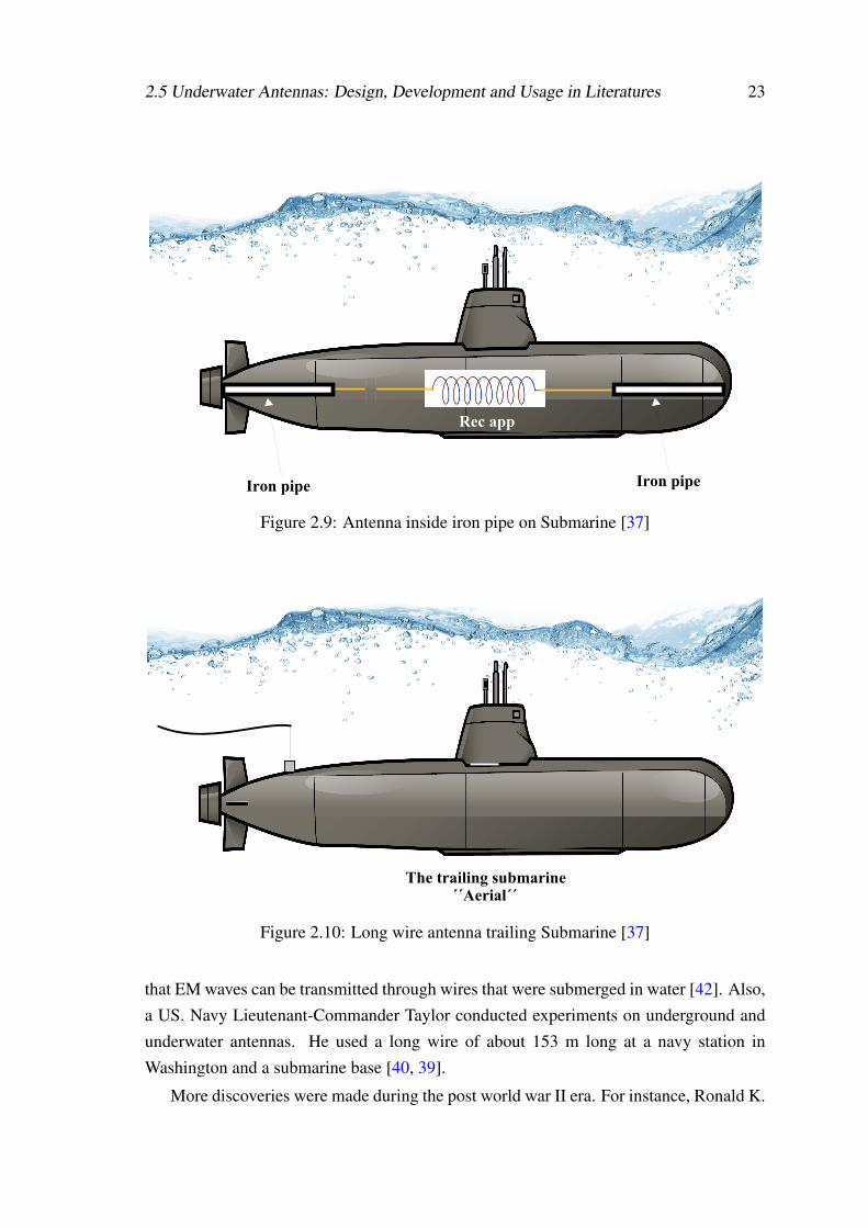
One of the earliest published work in an underwater antenna was by G. H. Clark in1909. His experiment consisted of, two wires of 9.2 m long which were connected tothe transmitting apparatus located at the Navy Yard Norfolk and also two insulated wiresof 5.2 m long submerged below the surface of water at the depth of 1.2 m located at theNavy Yard Washington were connected to the receiving apparatus through a condenserof capacity 0.003 microfarad. Signals were received by the receiver, which was around19 km away from the transmitter [36]. In furtherance of the work, experiments werealso conducted on a boat located near Norfolk. Here, copper plates were attached to theinsulated wires; while one plate was suspended over the stern into the water, the other wassuspended over the bow into the water. Signals transmitted from the Navy Yard in Norfolkwere received on this boat at a distance of up to 24 km. Despite the crude nature by whichthese experiments were conducted, it nonetheless became a remarkable achievement inthe history of underwater antenna communication [36]. J. H. Rogers similarly transmittedfrom boat with underwater wires to a station in his home in 1916 [36]. About threeyears after, Rogers produced what can be tagged resounding breakthrough in the usageof antennas for underwater application, which was written by H. W. Secor and titled"American Greatest War Invention". The inventor based his idea on what should be alogical relationship between wireless transmission and reception of radio signals in thesurface to those in the underwater environment. He believed that, since an antenna cantransmit signal from a high altitude platform (mast) to a receiving antenna at a designateddistance, then the same signal is transmitted appropriately through water, can be receivedby a receiving antenna submerged in underwater. In his work, he first used a heavilyinsulated stranded cable, stretched from stem to stern and attached to the submarines as areceiving antenna as presented in Fig. 2.8. This was later replaced by an insulated antennaplaced in iron pipes located inside the submarines, probably to protect the antenna fromthe effect of the medium as shown in Fig. 2.9. The third is a long wire antenna attachedto the last compartment of the submarine, thereby trailing it as presented in Fig. 2.10.
22 Review of Underwater Antennas: Designs, Developments and Usage
Based on these analyses and a couple of experiments, a wireless communication link wasestablished with the submarines placed in seawater. This invention became an importanttool that the American Navy used during the world war and the system he built paved waysfor research in the usage of antennas in underwater environments. It was also reportedthat the submarines must be at a distance of less than 10 km to the transmitting antennain seawater due to its conductive nature, whereas in fresh water the receiving antenna canbe at any depth [37].
Rec app
Insulated wire
Rec app
Grd´d on Hull Grd´d on Hull
Figure 2.8: Insulated wired antenna on Submarine [37]
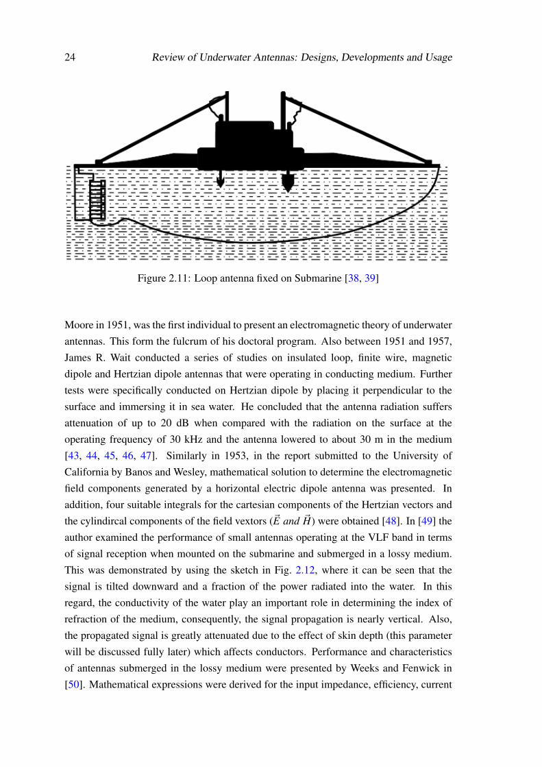
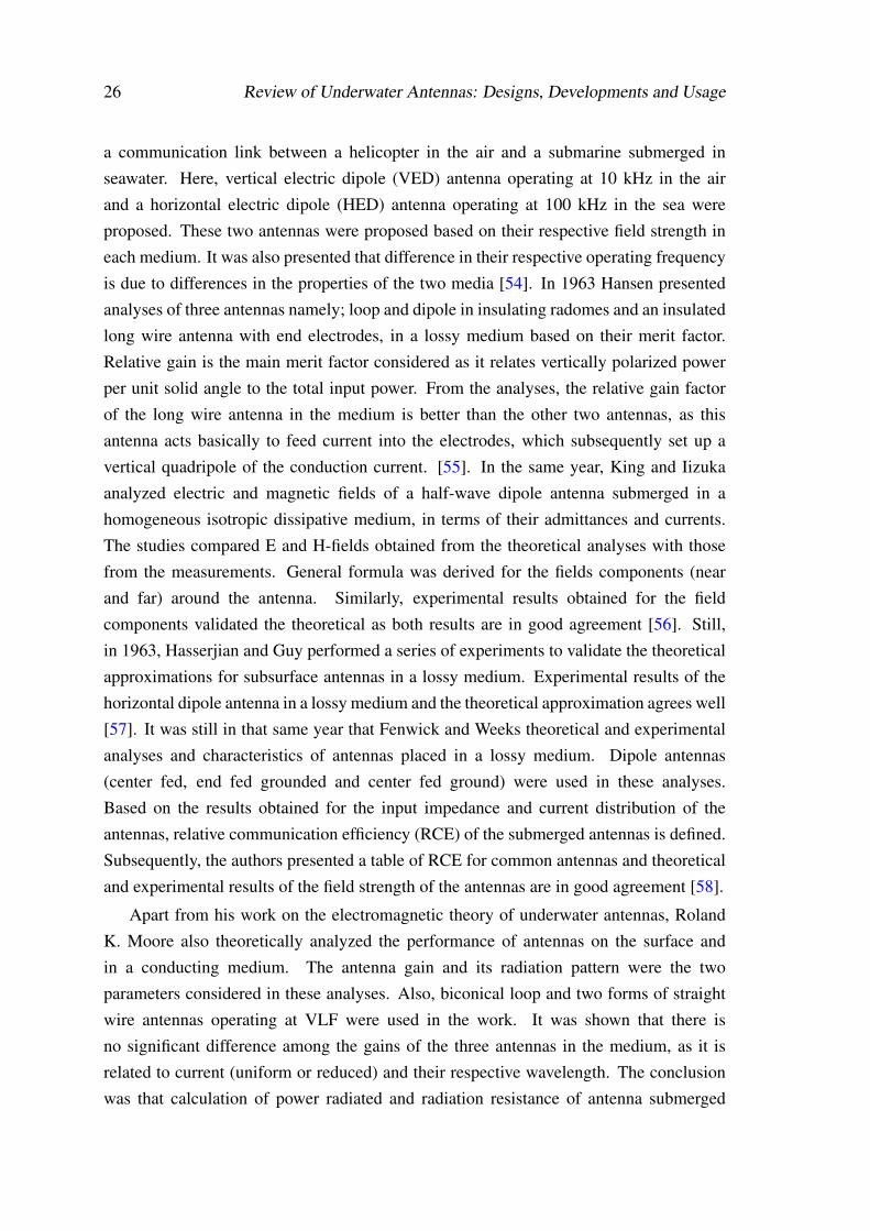
Shortly after Rogers’s invention, Willoughby and Lowell also in the same year,performed further experiments on the detection of submarines. They discovered thatloop antennas can likewise detect or receive radio signals transmitted through water[38, 39, 40]. The antenna system comprises of an insulated phosphorus bronze wirewhich was used to construct a single loop antenna that was firmly grounded by thehull of the submarine. This simply means hulls were part of the antenna and theprototype of their design is as presented in Fig. 2.11. The duo claimed that they wereable to successfully establish communication links between two submarines, which wereentirely submerged in seawater 20 Km apart at a wavelength of 952 m [38]. Thoughthe communication distance between the two submarines was later disputed by V. R.Fisher [41], it was obvious that the loop antenna was similarly used to establishedcommunication in seawater between two submarines. Around the same time frame, MajorGeneral George O. Squier conducted experiments where he used an insulated wire fortransmission of high-frequency signals through the water. His experiments confirmed
2.5 Underwater Antennas: Design, Development and Usage in Literatures 23
Iron pipe Iron pipe
Rec app
Figure 2.9: Antenna inside iron pipe on Submarine [37]
The trailing submarine ´´Aerial´´
Figure 2.10: Long wire antenna trailing Submarine [37]
that EM waves can be transmitted through wires that were submerged in water [42]. Also,a US. Navy Lieutenant-Commander Taylor conducted experiments on underground andunderwater antennas. He used a long wire of about 153 m long at a navy station inWashington and a submarine base [40, 39].
More discoveries were made during the post world war II era. For instance, Ronald K.
24 Review of Underwater Antennas: Designs, Developments and Usage
Figure 2.11: Loop antenna fixed on Submarine [38, 39]
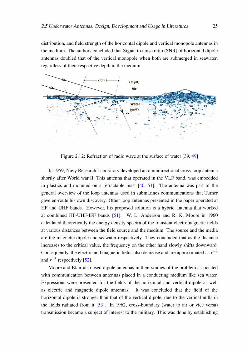
Moore in 1951, was the first individual to present an electromagnetic theory of underwaterantennas. This form the fulcrum of his doctoral program. Also between 1951 and 1957,James R. Wait conducted a series of studies on insulated loop, finite wire, magneticdipole and Hertzian dipole antennas that were operating in conducting medium. Furthertests were specifically conducted on Hertzian dipole by placing it perpendicular to thesurface and immersing it in sea water. He concluded that the antenna radiation suffersattenuation of up to 20 dB when compared with the radiation on the surface at theoperating frequency of 30 kHz and the antenna lowered to about 30 m in the medium[43, 44, 45, 46, 47]. Similarly in 1953, in the report submitted to the University ofCalifornia by Banos and Wesley, mathematical solution to determine the electromagneticfield components generated by a horizontal electric dipole antenna was presented. Inaddition, four suitable integrals for the cartesian components of the Hertzian vectors andthe cylindircal components of the field vextors (~E and ~H) were obtained [48]. In [49] theauthor examined the performance of small antennas operating at the VLF band in termsof signal reception when mounted on the submarine and submerged in a lossy medium.This was demonstrated by using the sketch in Fig. 2.12, where it can be seen that thesignal is tilted downward and a fraction of the power radiated into the water. In thisregard, the conductivity of the water play an important role in determining the index ofrefraction of the medium, consequently, the signal propagation is nearly vertical. Also,the propagated signal is greatly attenuated due to the effect of skin depth (this parameterwill be discussed fully later) which affects conductors. Performance and characteristicsof antennas submerged in the lossy medium were presented by Weeks and Fenwick in[50]. Mathematical expressions were derived for the input impedance, efficiency, current
2.5 Underwater Antennas: Design, Development and Usage in Literatures 25
distribution, and field strength of the horizontal dipole and vertical monopole antennas inthe medium. The authors concluded that Signal to noise ratio (SNR) of horizontal dipoleantennas doubled that of the vertical monopole when both are submerged in seawater,regardless of their respective depth in the medium.
Water
Air
l/(2p) (e0m0)
(sm0)d
Figure 2.12: Refraction of radio wave at the surface of water [39, 49]
In 1959, Navy Research Laboratory developed an omnidirectional cross-loop antennashortly after World war II. This antenna that operated in the VLF band, was embeddedin plastics and mounted on a retractable mast [40, 51]. The antenna was part of thegeneral overview of the loop antennas used in submarines communications that Turnergave en-route his own discovery. Other loop antennas presented in the paper operated atHF and UHF bands. However, his proposed solution is a hybrid antenna that workedat combined HF-UHF-IFF bands [51]. W. L. Anderson and R. K. Moore in 1960calculated theoretically the energy density spectra of the transient electromagnetic fieldsat various distances between the field source and the medium. The source and the mediaare the magnetic dipole and seawater respectively. They concluded that as the distanceincreases to the critical value, the frequency on the other hand slowly shifts downward.Consequently, the electric and magnetic fields also decrease and are approximated as r−2
and r−3 respectively [52].
Moore and Blair also used dipole antennas in their studies of the problem associatedwith communication between antennas placed in a conducting medium like sea water.Expressions were presented for the fields of the horizontal and vertical dipole as wellas electric and magnetic dipole antennas. It was concluded that the field of thehorizontal dipole is stronger than that of the vertical dipole, due to the vertical nulls inthe fields radiated from it [53]. In 1962, cross-boundary (water to air or vice versa)transmission became a subject of interest to the military. This was done by establishing
26 Review of Underwater Antennas: Designs, Developments and Usage
a communication link between a helicopter in the air and a submarine submerged inseawater. Here, vertical electric dipole (VED) antenna operating at 10 kHz in the airand a horizontal electric dipole (HED) antenna operating at 100 kHz in the sea wereproposed. These two antennas were proposed based on their respective field strength ineach medium. It was also presented that difference in their respective operating frequencyis due to differences in the properties of the two media [54]. In 1963 Hansen presentedanalyses of three antennas namely; loop and dipole in insulating radomes and an insulatedlong wire antenna with end electrodes, in a lossy medium based on their merit factor.Relative gain is the main merit factor considered as it relates vertically polarized powerper unit solid angle to the total input power. From the analyses, the relative gain factorof the long wire antenna in the medium is better than the other two antennas, as thisantenna acts basically to feed current into the electrodes, which subsequently set up avertical quadripole of the conduction current. [55]. In the same year, King and Iizukaanalyzed electric and magnetic fields of a half-wave dipole antenna submerged in ahomogeneous isotropic dissipative medium, in terms of their admittances and currents.The studies compared E and H-fields obtained from the theoretical analyses with thosefrom the measurements. General formula was derived for the fields components (nearand far) around the antenna. Similarly, experimental results obtained for the fieldcomponents validated the theoretical as both results are in good agreement [56]. Still,in 1963, Hasserjian and Guy performed a series of experiments to validate the theoreticalapproximations for subsurface antennas in a lossy medium. Experimental results of thehorizontal dipole antenna in a lossy medium and the theoretical approximation agrees well[57]. It was still in that same year that Fenwick and Weeks theoretical and experimentalanalyses and characteristics of antennas placed in a lossy medium. Dipole antennas(center fed, end fed grounded and center fed ground) were used in these analyses.Based on the results obtained for the input impedance and current distribution of theantennas, relative communication efficiency (RCE) of the submerged antennas is defined.Subsequently, the authors presented a table of RCE for common antennas and theoreticaland experimental results of the field strength of the antennas are in good agreement [58].
Apart from his work on the electromagnetic theory of underwater antennas, RolandK. Moore also theoretically analyzed the performance of antennas on the surface andin a conducting medium. The antenna gain and its radiation pattern were the twoparameters considered in these analyses. Also, biconical loop and two forms of straightwire antennas operating at VLF were used in the work. It was shown that there isno significant difference among the gains of the three antennas in the medium, as it isrelated to current (uniform or reduced) and their respective wavelength. The conclusionwas that calculation of power radiated and radiation resistance of antenna submerged
2.5 Underwater Antennas: Design, Development and Usage in Literatures 27
in a conducting medium is dissimilar to the calculation for the same antenna in theair. In addition, the gain and radiation pattern of the antennas in this medium wereaffected by the energy dissipated in the medium [59]. Based on these results, extensiveeffort was made by the author on the propagation of radio communication in sea water.Three proposed communication links for antennas submerged in the sea water and wereused in his experiments, these are; surface to submarine communication, submarine tosubmarine communication via surface and submarine to surface communication. It wasdemonstrated that if the antenna is lowered into depth of within 5 meters to the surface andthe bandwidth not exceeding 1 Hz, a propagation range of up to 20 km can be achieved.In conclusion, it was stated that propagation in seawater will require antennas operatingat VLF bands (precisely at frequencies well below 10 kHz) due to strong attenuation inthe medium. Also, propagation distances (communication ranges) are affected by depthattenuation and atmospheric noise. The author finally submitted that communication linkbetween surface vessels and ocean-bottom working parties could be established by usageof antennas operating at ELF bands [60]. In furtherance of the research on cross-boundarycommunications, Durrani in 1964 presented the study on the usage of the magnetic dipolessubmerged in the sea water. In the paper, the theoretical analysis including the electricand magnetic components of the horizontal magnetic dipole (HMD) and vertical magneticdipole (VMD) was thoroughly discussed. Also, undersea fields produced by differentdipoles compared and it was concluded that electric and magnetic fields produced atlarge distances by HMD in the medium are stronger than those by VMD with the sameexcitation and size. Similarly, for a large number of turns, equal currents, and equal inputpowers, HMD still showing a superior performance over VMD [61]. In 1969, King et alpresented theoretical analyses of the current, distribution of charge and the admittanceof cylindrical antennas immersed in arbitrary homogeneous media, with the effectiveconductivity of the media greater than or equal to zero. Electrically short, half-wave andfull wave dipole antennas were used in these analyses. The theoretical results obtainedfor the three antennas were compared with the measurement and the two shows goodagreement [62].
A year later the work was extended basically to determine the EM fields of linearantennas immersed in the Atlantic ocean or buried in the earth. Here, three subdivisionsof horizontal ranges were used to determine a measurement of EM fields in the dissipativemedium. These are; the near field range, the intermediate range, and the asymptotic range.Finally, the numerical solutions were simulated and the results were compared with theresults of the experiments. In their submission, experimental measurements of the fieldsin the near and intermediate field range matched the predicted results in the medium[63]. Also in 1971, Tsao derived an expression to determine the radiation resistance
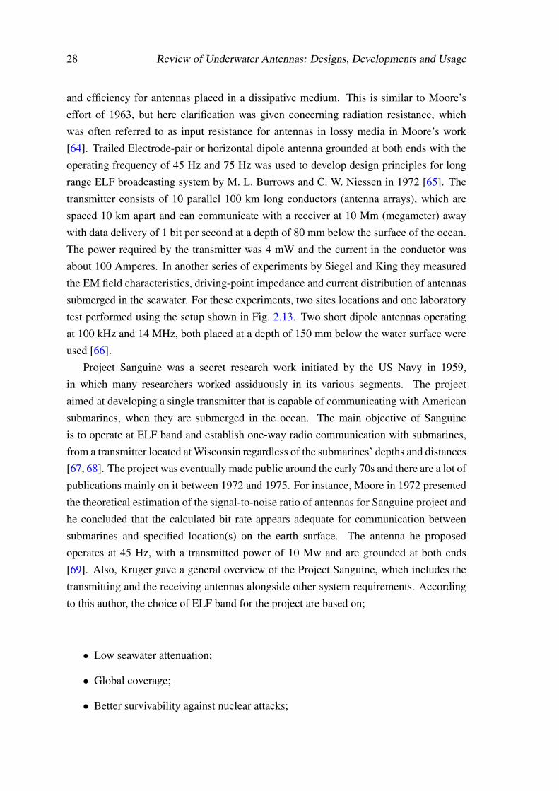
28 Review of Underwater Antennas: Designs, Developments and Usage
and efficiency for antennas placed in a dissipative medium. This is similar to Moore’seffort of 1963, but here clarification was given concerning radiation resistance, whichwas often referred to as input resistance for antennas in lossy media in Moore’s work[64]. Trailed Electrode-pair or horizontal dipole antenna grounded at both ends with theoperating frequency of 45 Hz and 75 Hz was used to develop design principles for longrange ELF broadcasting system by M. L. Burrows and C. W. Niessen in 1972 [65]. Thetransmitter consists of 10 parallel 100 km long conductors (antenna arrays), which arespaced 10 km apart and can communicate with a receiver at 10 Mm (megameter) awaywith data delivery of 1 bit per second at a depth of 80 mm below the surface of the ocean.The power required by the transmitter was 4 mW and the current in the conductor wasabout 100 Amperes. In another series of experiments by Siegel and King they measuredthe EM field characteristics, driving-point impedance and current distribution of antennassubmerged in the seawater. For these experiments, two sites locations and one laboratorytest performed using the setup shown in Fig. 2.13. Two short dipole antennas operatingat 100 kHz and 14 MHz, both placed at a depth of 150 mm below the water surface wereused [66].
Project Sanguine was a secret research work initiated by the US Navy in 1959,in which many researchers worked assiduously in its various segments. The projectaimed at developing a single transmitter that is capable of communicating with Americansubmarines, when they are submerged in the ocean. The main objective of Sanguineis to operate at ELF band and establish one-way radio communication with submarines,from a transmitter located at Wisconsin regardless of the submarines’ depths and distances[67, 68]. The project was eventually made public around the early 70s and there are a lot ofpublications mainly on it between 1972 and 1975. For instance, Moore in 1972 presentedthe theoretical estimation of the signal-to-noise ratio of antennas for Sanguine project andhe concluded that the calculated bit rate appears adequate for communication betweensubmarines and specified location(s) on the earth surface. The antenna he proposedoperates at 45 Hz, with a transmitted power of 10 Mw and are grounded at both ends[69]. Also, Kruger gave a general overview of the Project Sanguine, which includes thetransmitting and the receiving antennas alongside other system requirements. Accordingto this author, the choice of ELF band for the project are based on;
• Low seawater attenuation;
• Global coverage;
• Better survivability against nuclear attacks;
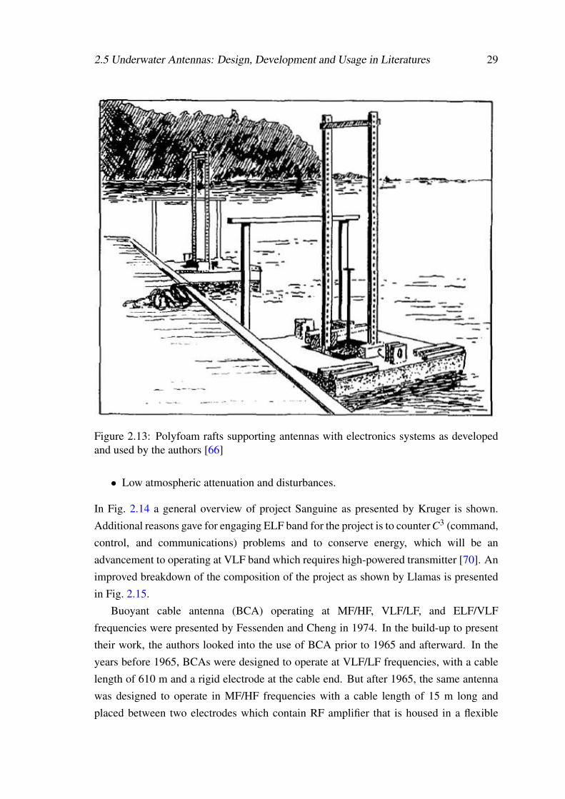
2.5 Underwater Antennas: Design, Development and Usage in Literatures 29
Figure 2.13: Polyfoam rafts supporting antennas with electronics systems as developedand used by the authors [66]
• Low atmospheric attenuation and disturbances.
In Fig. 2.14 a general overview of project Sanguine as presented by Kruger is shown.Additional reasons gave for engaging ELF band for the project is to counter C3 (command,control, and communications) problems and to conserve energy, which will be anadvancement to operating at VLF band which requires high-powered transmitter [70]. Animproved breakdown of the composition of the project as shown by Llamas is presentedin Fig. 2.15.
Buoyant cable antenna (BCA) operating at MF/HF, VLF/LF, and ELF/VLFfrequencies were presented by Fessenden and Cheng in 1974. In the build-up to presenttheir work, the authors looked into the use of BCA prior to 1965 and afterward. In theyears before 1965, BCAs were designed to operate at VLF/LF frequencies, with a cablelength of 610 m and a rigid electrode at the cable end. But after 1965, the same antennawas designed to operate in MF/HF frequencies with a cable length of 15 m long andplaced between two electrodes which contain RF amplifier that is housed in a flexible
30 Review of Underwater Antennas: Designs, Developments and Usage
Figure 2.14: General overview of Project Sanguine [70]
Figure 2.15: The proposed project Sanguine by U.S. Navy [39]
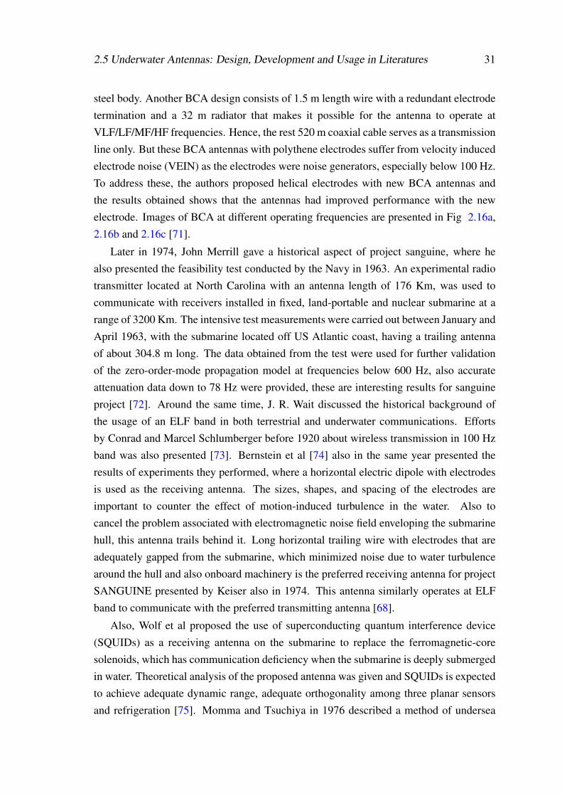
2.5 Underwater Antennas: Design, Development and Usage in Literatures 31
steel body. Another BCA design consists of 1.5 m length wire with a redundant electrodetermination and a 32 m radiator that makes it possible for the antenna to operate atVLF/LF/MF/HF frequencies. Hence, the rest 520 m coaxial cable serves as a transmissionline only. But these BCA antennas with polythene electrodes suffer from velocity inducedelectrode noise (VEIN) as the electrodes were noise generators, especially below 100 Hz.To address these, the authors proposed helical electrodes with new BCA antennas andthe results obtained shows that the antennas had improved performance with the newelectrode. Images of BCA at different operating frequencies are presented in Fig 2.16a,2.16b and 2.16c [71].
Later in 1974, John Merrill gave a historical aspect of project sanguine, where healso presented the feasibility test conducted by the Navy in 1963. An experimental radiotransmitter located at North Carolina with an antenna length of 176 Km, was used tocommunicate with receivers installed in fixed, land-portable and nuclear submarine at arange of 3200 Km. The intensive test measurements were carried out between January andApril 1963, with the submarine located off US Atlantic coast, having a trailing antennaof about 304.8 m long. The data obtained from the test were used for further validationof the zero-order-mode propagation model at frequencies below 600 Hz, also accurateattenuation data down to 78 Hz were provided, these are interesting results for sanguineproject [72]. Around the same time, J. R. Wait discussed the historical background ofthe usage of an ELF band in both terrestrial and underwater communications. Effortsby Conrad and Marcel Schlumberger before 1920 about wireless transmission in 100 Hzband was also presented [73]. Bernstein et al [74] also in the same year presented theresults of experiments they performed, where a horizontal electric dipole with electrodesis used as the receiving antenna. The sizes, shapes, and spacing of the electrodes areimportant to counter the effect of motion-induced turbulence in the water. Also tocancel the problem associated with electromagnetic noise field enveloping the submarinehull, this antenna trails behind it. Long horizontal trailing wire with electrodes that areadequately gapped from the submarine, which minimized noise due to water turbulencearound the hull and also onboard machinery is the preferred receiving antenna for projectSANGUINE presented by Keiser also in 1974. This antenna similarly operates at ELFband to communicate with the preferred transmitting antenna [68].
Also, Wolf et al proposed the use of superconducting quantum interference device(SQUIDs) as a receiving antenna on the submarine to replace the ferromagnetic-coresolenoids, which has communication deficiency when the submarine is deeply submergedin water. Theoretical analysis of the proposed antenna was given and SQUIDs is expectedto achieve adequate dynamic range, adequate orthogonality among three planar sensorsand refrigeration [75]. Momma and Tsuchiya in 1976 described a method of undersea
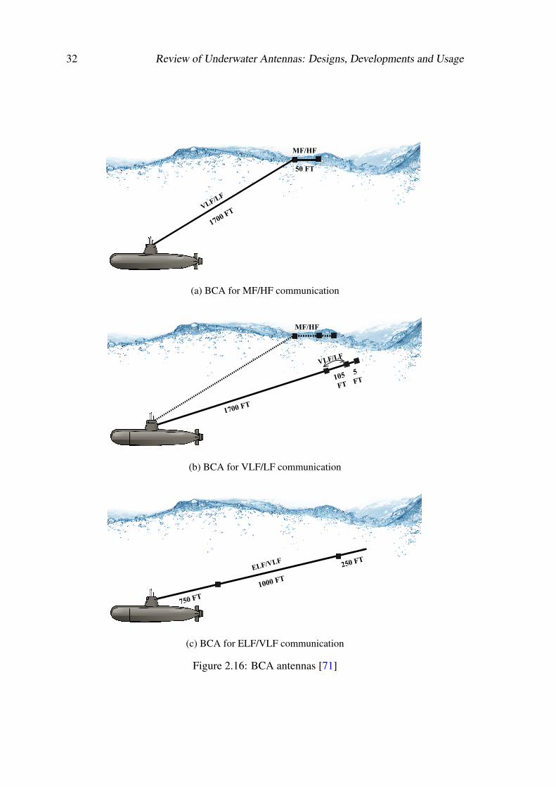
32 Review of Underwater Antennas: Designs, Developments and Usage
VLF/LF
1700 FT
MF/HF
50 FT
(a) BCA for MF/HF communication
MF/HF
1700 FT
105
FT
5 FT
VLF/LF
(b) BCA for VLF/LF communication
ELF/VLF
1000 FT
750 FT
250 FT
(c) BCA for ELF/VLF communication
Figure 2.16: BCA antennas [71]
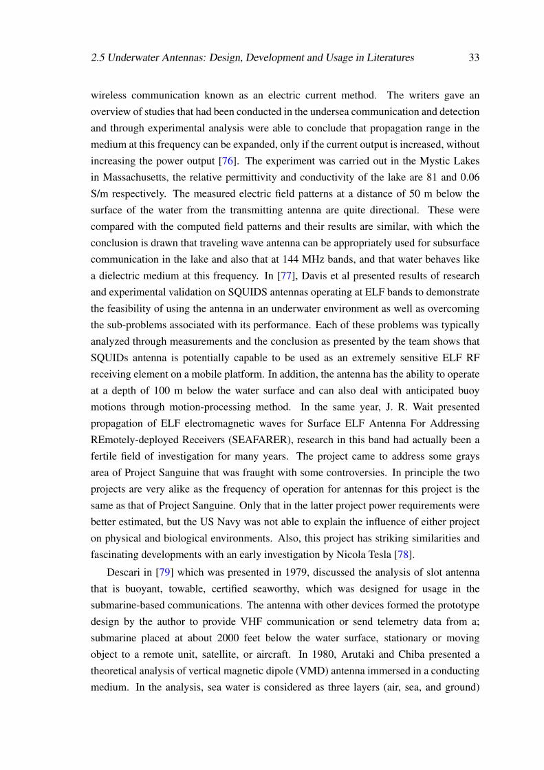
2.5 Underwater Antennas: Design, Development and Usage in Literatures 33
wireless communication known as an electric current method. The writers gave anoverview of studies that had been conducted in the undersea communication and detectionand through experimental analysis were able to conclude that propagation range in themedium at this frequency can be expanded, only if the current output is increased, withoutincreasing the power output [76]. The experiment was carried out in the Mystic Lakesin Massachusetts, the relative permittivity and conductivity of the lake are 81 and 0.06S/m respectively. The measured electric field patterns at a distance of 50 m below thesurface of the water from the transmitting antenna are quite directional. These werecompared with the computed field patterns and their results are similar, with which theconclusion is drawn that traveling wave antenna can be appropriately used for subsurfacecommunication in the lake and also that at 144 MHz bands, and that water behaves likea dielectric medium at this frequency. In [77], Davis et al presented results of researchand experimental validation on SQUIDS antennas operating at ELF bands to demonstratethe feasibility of using the antenna in an underwater environment as well as overcomingthe sub-problems associated with its performance. Each of these problems was typicallyanalyzed through measurements and the conclusion as presented by the team shows thatSQUIDs antenna is potentially capable to be used as an extremely sensitive ELF RFreceiving element on a mobile platform. In addition, the antenna has the ability to operateat a depth of 100 m below the water surface and can also deal with anticipated buoymotions through motion-processing method. In the same year, J. R. Wait presentedpropagation of ELF electromagnetic waves for Surface ELF Antenna For AddressingREmotely-deployed Receivers (SEAFARER), research in this band had actually been afertile field of investigation for many years. The project came to address some graysarea of Project Sanguine that was fraught with some controversies. In principle the twoprojects are very alike as the frequency of operation for antennas for this project is thesame as that of Project Sanguine. Only that in the latter project power requirements werebetter estimated, but the US Navy was not able to explain the influence of either projecton physical and biological environments. Also, this project has striking similarities andfascinating developments with an early investigation by Nicola Tesla [78].
Descari in [79] which was presented in 1979, discussed the analysis of slot antennathat is buoyant, towable, certified seaworthy, which was designed for usage in thesubmarine-based communications. The antenna with other devices formed the prototypedesign by the author to provide VHF communication or send telemetry data from a;submarine placed at about 2000 feet below the water surface, stationary or movingobject to a remote unit, satellite, or aircraft. In 1980, Arutaki and Chiba presented atheoretical analysis of vertical magnetic dipole (VMD) antenna immersed in a conductingmedium. In the analysis, sea water is considered as three layers (air, sea, and ground)
34 Review of Underwater Antennas: Designs, Developments and Usage
media with which communication was established between the antenna and object inair, sea, and ground (seabed). The dominant term in their results agrees with Moore’sresults and they concluded that the VMD antenna is more advantageous for this typeof communication than horizontal loop antenna [80]. Michael B. Callaham in 1981described the transmission and reception of signals by submarines were mainly beendone through UHF and VHF frequencies [81]. But the author also quick to point out thattransmitting and receiving at these frequencies will require either deployment of smallmast antenna that will remain above water surface or the entire submarine coming nearthe surface. In either case, it may be risky for the operation of the underwater bodiesas it will mean exposing them to detection by enemies. Thus, for total concealment ofthe location of submarines from enemy’s view, the author proved that communicating inELF and ULF bands as well as through optical transmission will guarantee the signalpenetrating deeply into the water. Thereby ensuring full protection of the submarinesfrom any attacks.
In revealing the interest of British government to build a transmitter operating at ELFband and communicating with submarines, D. L. Jones recapped the developments insubmarine communications over three decades which include; the danger of using VLFfrequencies in communicating with submarines, different antennas that were designedto operate at required operating frequencies for deep-sea submarine communicationsand eventual breakthrough through ELF band, which made transmission and receptionpossible in tens of kilometers below the sea surface. References were made particularlyto various stages of involvement of Project Sanguine, which was later upgraded toSeafarer [82]. Lloyd Butler in 1987 showed the importance of underwater communicationto amateur radio by posing the following questions; How far can we communicateunderwater in the sea or in a lake [83]. How large is the signal attenuation and whatFrequency can be used? Could we use 1.8 MHz? These questions were answered throughboth theoretical and experimental results that were presented in his work. It was thereforeaffirmed that attenuation increases with increasing operating frequency, which is about46 dB at 1.8 MHz in sea water and 27 dB in fresh water. It was also revealed thatcross-boundary interface transmission will be very difficult in this band, as the attenuationin the outbound signal (water to air) and the inbound (air to water) add up to 54 dB in freshwater as shown in Fig. 2.17.
Dunbar gave two broad classes of antennas that can be used for subseacommunications. These are the magnetic field loop (MFL) and electric field line (EFL)antennas. These were also known as passive reciprocal devices (can be used as eithertransmitting or receiving antennas). This is in contrast with SQUID, fluxgate and halleffect antennas that are only suited for receiving applications. examples of these antennas
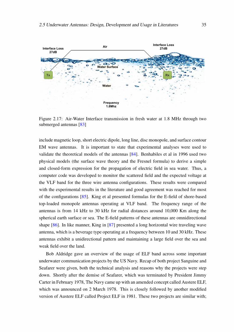
2.5 Underwater Antennas: Design, Development and Usage in Literatures 35
Water
Water Surface
Air
Frequency 1.8Mhz
Tx Rx
Interface Loss 27dBInterface Loss
27dB
Figure 2.17: Air-Water Interface transmission in fresh water at 1.8 MHz through twosubmerged antennas [83]
include magnetic loop, short electric dipole, long line, disc monopole, and surface contourEM wave antennas. It is important to state that experimental analyses were used tovalidate the theoretical models of the antennas [84]. Benhabiles et al in 1996 used twophysical models (the surface wave theory and the Fresnel formula) to derive a simpleand closed-form expression for the propagation of electric field in sea water. Thus, acomputer code was developed to monitor the scattered field and the expected voltage atthe VLF band for the three wire antenna configurations. These results were comparedwith the experimental results in the literature and good agreement was reached for mostof the configurations [85]. King et al presented formulas for the E-field of shore-basedtop-loaded monopole antennas operating at VLF band. The frequency range of theantennas is from 14 kHz to 30 kHz for radial distances around 10,000 Km along thespherical earth surface or sea. The E-field patterns of these antennas are omnidirectionalshape [86]. In like manner, King in [87] presented a long horizontal wire traveling waveantenna, which is a beverage type operating at a frequency between 10 and 30 kHz. Theseantennas exhibit a unidirectional pattern and maintaining a large field over the sea andweak field over the land.
Bob Aldridge gave an overview of the usage of ELF band across some importantunderwater communication projects by the US Navy. Recap of both project Sanguine andSeafarer were given, both the technical analysis and reasons why the projects were stepdown. Shortly after the demise of Seafarer, which was terminated by President JimmyCarter in February 1978, The Navy came up with an amended concept called Austere ELF,which was announced on 2 March 1978. This is closely followed by another modifiedversion of Austere ELF called Project ELF in 1981. These two projects are similar with;
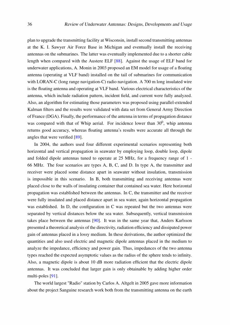
36 Review of Underwater Antennas: Designs, Developments and Usage
plan to upgrade the transmitting facility at Wisconsin, install second transmitting antennasat the K. I. Sawyer Air Force Base in Michigan and eventually install the receivingantennas on the submarines. The latter was eventually implemented due to a shorter cablelength when compared with the Austere ELF [88]. Against the usage of ELF band forunderwater applications, A. Monin in 2003 proposed an EM model for usage of a floatingantenna (operating at VLF band) installed on the tail of submarines for communicationwith LORAN-C (long range navigation-C) radio navigation. A 700 m long insulated wireis the floating antenna and operating at VLF band. Various electrical characteristics of theantenna, which include radiation pattern, incident field, and current were fully analyzed.Also, an algorithm for estimating those parameters was proposed using parallel-extendedKalman filters and the results were validated with data set from General Army Directionof France (DGA). Finally, the performance of the antenna in terms of propagation distancewas compared with that of Whip aerial. For incidence lower than 300, whip antennareturns good accuracy, whereas floating antenna’s results were accurate all through theangles that were verified [89].
In 2004, the authors used four different experimental scenarios representing bothhorizontal and vertical propagation in seawater by employing loop, double loop, dipoleand folded dipole antennas tuned to operate at 25 MHz, for a frequency range of 1 -66 MHz. The four scenarios are types A, B, C, and D. In type A, the transmitter andreceiver were placed some distance apart in seawater without insulation, transmissionis impossible in this scenario. In B, both transmitting and receiving antennas wereplaced close to the walls of insulating container that contained sea water. Here horizontalpropagation was established between the antennas. In C, the transmitter and the receiverwere fully insulated and placed distance apart in sea water, again horizontal propagationwas established. In D, the configuration in C was repeated but the two antennas wereseparated by vertical distances below the sea water. Subsequently, vertical transmissiontakes place between the antennas [90]. It was in the same year that, Anders Karlssonpresented a theoretical analysis of the directivity, radiation efficiency and dissipated powergain of antennas placed in a lossy medium. In these derivations, the author optimized thequantities and also used electric and magnetic dipole antennas placed in the medium toanalyze the impedance, efficiency and power gain. Thus, impedances of the two antennatypes reached the expected asymptotic values as the radius of the sphere tends to infinity.Also, a magnetic dipole is about 10 dB more radiation efficient that the electric dipoleantennas. It was concluded that larger gain is only obtainable by adding higher ordermulti-poles [91].
The world largest "Radio" station by Carlos A. Altgelt in 2005 gave more informationabout the project Sanguine research work both from the transmitting antenna on the earth
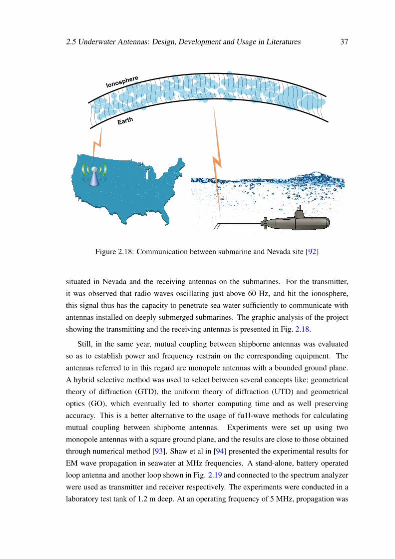
2.5 Underwater Antennas: Design, Development and Usage in Literatures 37
Earth
Ionospher
e
Figure 2.18: Communication between submarine and Nevada site [92]
situated in Nevada and the receiving antennas on the submarines. For the transmitter,it was observed that radio waves oscillating just above 60 Hz, and hit the ionosphere,this signal thus has the capacity to penetrate sea water sufficiently to communicate withantennas installed on deeply submerged submarines. The graphic analysis of the projectshowing the transmitting and the receiving antennas is presented in Fig. 2.18.
Still, in the same year, mutual coupling between shipborne antennas was evaluatedso as to establish power and frequency restrain on the corresponding equipment. Theantennas referred to in this regard are monopole antennas with a bounded ground plane.A hybrid selective method was used to select between several concepts like; geometricaltheory of diffraction (GTD), the uniform theory of diffraction (UTD) and geometricaloptics (GO), which eventually led to shorter computing time and as well preservingaccuracy. This is a better alternative to the usage of fu1l-wave methods for calculatingmutual coupling between shipborne antennas. Experiments were set up using twomonopole antennas with a square ground plane, and the results are close to those obtainedthrough numerical method [93]. Shaw et al in [94] presented the experimental results forEM wave propagation in seawater at MHz frequencies. A stand-alone, battery operatedloop antenna and another loop shown in Fig. 2.19 and connected to the spectrum analyzerwere used as transmitter and receiver respectively. The experiments were conducted in alaboratory test tank of 1.2 m deep. At an operating frequency of 5 MHz, propagation was
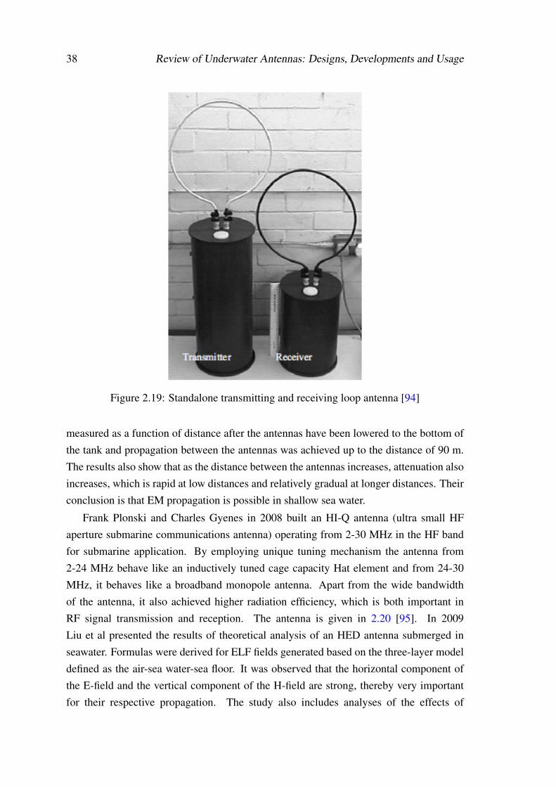
38 Review of Underwater Antennas: Designs, Developments and Usage
Figure 2.19: Standalone transmitting and receiving loop antenna [94]
measured as a function of distance after the antennas have been lowered to the bottom ofthe tank and propagation between the antennas was achieved up to the distance of 90 m.The results also show that as the distance between the antennas increases, attenuation alsoincreases, which is rapid at low distances and relatively gradual at longer distances. Theirconclusion is that EM propagation is possible in shallow sea water.
Frank Plonski and Charles Gyenes in 2008 built an HI-Q antenna (ultra small HFaperture submarine communications antenna) operating from 2-30 MHz in the HF bandfor submarine application. By employing unique tuning mechanism the antenna from2-24 MHz behave like an inductively tuned cage capacity Hat element and from 24-30MHz, it behaves like a broadband monopole antenna. Apart from the wide bandwidthof the antenna, it also achieved higher radiation efficiency, which is both important inRF signal transmission and reception. The antenna is given in 2.20 [95]. In 2009Liu et al presented the results of theoretical analysis of an HED antenna submerged inseawater. Formulas were derived for ELF fields generated based on the three-layer modeldefined as the air-sea water-sea floor. It was observed that the horizontal component ofthe E-field and the vertical component of the H-field are strong, thereby very importantfor their respective propagation. The study also includes analyses of the effects of
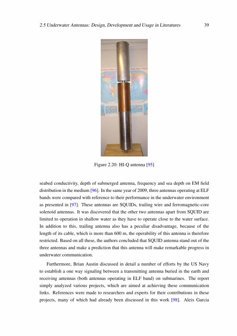
2.5 Underwater Antennas: Design, Development and Usage in Literatures 39
Figure 2.20: HI-Q antenna [95]
seabed conductivity, depth of submerged antenna, frequency and sea depth on EM fielddistribution in the medium [96]. In the same year of 2009, three antennas operating at ELFbands were compared with reference to their performance in the underwater environmentas presented in [97]. These antennas are SQUIDs, trailing wire and ferromagnetic-coresolenoid antennas. It was discovered that the other two antennas apart from SQUID arelimited to operation in shallow water as they have to operate close to the water surface.In addition to this, trailing antenna also has a peculiar disadvantage, because of thelength of its cable, which is more than 600 m, the operability of this antenna is thereforerestricted. Based on all these, the authors concluded that SQUID antenna stand out of thethree antennas and make a prediction that this antenna will make remarkable progress inunderwater communication.
Furthermore, Brian Austin discussed in detail a number of efforts by the US Navyto establish a one way signaling between a transmitting antenna buried in the earth andreceiving antennas (both antennas operating in ELF band) on submarines. The reportsimply analyzed various projects, which are aimed at achieving these communicationlinks. References were made to researchers and experts for their contributions in theseprojects, many of which had already been discussed in this work [98]. Aleix Garcia
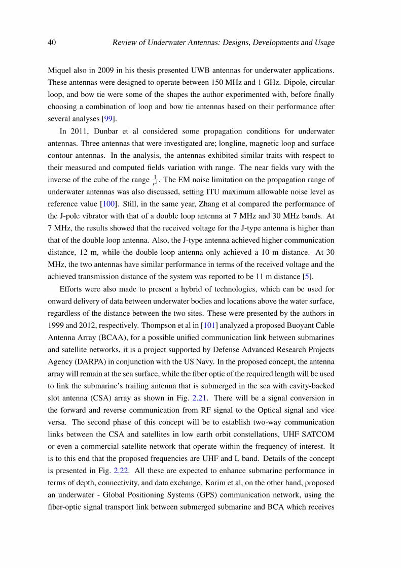
40 Review of Underwater Antennas: Designs, Developments and Usage
Miquel also in 2009 in his thesis presented UWB antennas for underwater applications.These antennas were designed to operate between 150 MHz and 1 GHz. Dipole, circularloop, and bow tie were some of the shapes the author experimented with, before finallychoosing a combination of loop and bow tie antennas based on their performance afterseveral analyses [99].
In 2011, Dunbar et al considered some propagation conditions for underwaterantennas. Three antennas that were investigated are; longline, magnetic loop and surfacecontour antennas. In the analysis, the antennas exhibited similar traits with respect totheir measured and computed fields variation with range. The near fields vary with theinverse of the cube of the range 1
r3 . The EM noise limitation on the propagation range ofunderwater antennas was also discussed, setting ITU maximum allowable noise level asreference value [100]. Still, in the same year, Zhang et al compared the performance ofthe J-pole vibrator with that of a double loop antenna at 7 MHz and 30 MHz bands. At7 MHz, the results showed that the received voltage for the J-type antenna is higher thanthat of the double loop antenna. Also, the J-type antenna achieved higher communicationdistance, 12 m, while the double loop antenna only achieved a 10 m distance. At 30MHz, the two antennas have similar performance in terms of the received voltage and theachieved transmission distance of the system was reported to be 11 m distance [5].
Efforts were also made to present a hybrid of technologies, which can be used foronward delivery of data between underwater bodies and locations above the water surface,regardless of the distance between the two sites. These were presented by the authors in1999 and 2012, respectively. Thompson et al in [101] analyzed a proposed Buoyant CableAntenna Array (BCAA), for a possible unified communication link between submarinesand satellite networks, it is a project supported by Defense Advanced Research ProjectsAgency (DARPA) in conjunction with the US Navy. In the proposed concept, the antennaarray will remain at the sea surface, while the fiber optic of the required length will be usedto link the submarine’s trailing antenna that is submerged in the sea with cavity-backedslot antenna (CSA) array as shown in Fig. 2.21. There will be a signal conversion inthe forward and reverse communication from RF signal to the Optical signal and viceversa. The second phase of this concept will be to establish two-way communicationlinks between the CSA and satellites in low earth orbit constellations, UHF SATCOMor even a commercial satellite network that operate within the frequency of interest. Itis to this end that the proposed frequencies are UHF and L band. Details of the conceptis presented in Fig. 2.22. All these are expected to enhance submarine performance interms of depth, connectivity, and data exchange. Karim et al, on the other hand, proposedan underwater - Global Positioning Systems (GPS) communication network, using thefiber-optic signal transport link between submerged submarine and BCA which receives
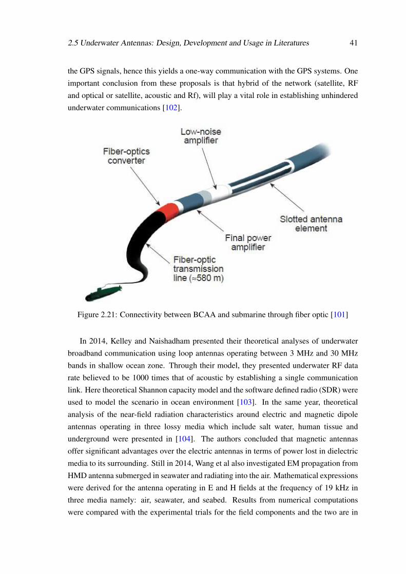
2.5 Underwater Antennas: Design, Development and Usage in Literatures 41
the GPS signals, hence this yields a one-way communication with the GPS systems. Oneimportant conclusion from these proposals is that hybrid of the network (satellite, RFand optical or satellite, acoustic and Rf), will play a vital role in establishing unhinderedunderwater communications [102].
Figure 2.21: Connectivity between BCAA and submarine through fiber optic [101]
In 2014, Kelley and Naishadham presented their theoretical analyses of underwaterbroadband communication using loop antennas operating between 3 MHz and 30 MHzbands in shallow ocean zone. Through their model, they presented underwater RF datarate believed to be 1000 times that of acoustic by establishing a single communicationlink. Here theoretical Shannon capacity model and the software defined radio (SDR) wereused to model the scenario in ocean environment [103]. In the same year, theoreticalanalysis of the near-field radiation characteristics around electric and magnetic dipoleantennas operating in three lossy media which include salt water, human tissue andunderground were presented in [104]. The authors concluded that magnetic antennasoffer significant advantages over the electric antennas in terms of power lost in dielectricmedia to its surrounding. Still in 2014, Wang et al also investigated EM propagation fromHMD antenna submerged in seawater and radiating into the air. Mathematical expressionswere derived for the antenna operating in E and H fields at the frequency of 19 kHz inthree media namely: air, seawater, and seabed. Results from numerical computationswere compared with the experimental trials for the field components and the two are in
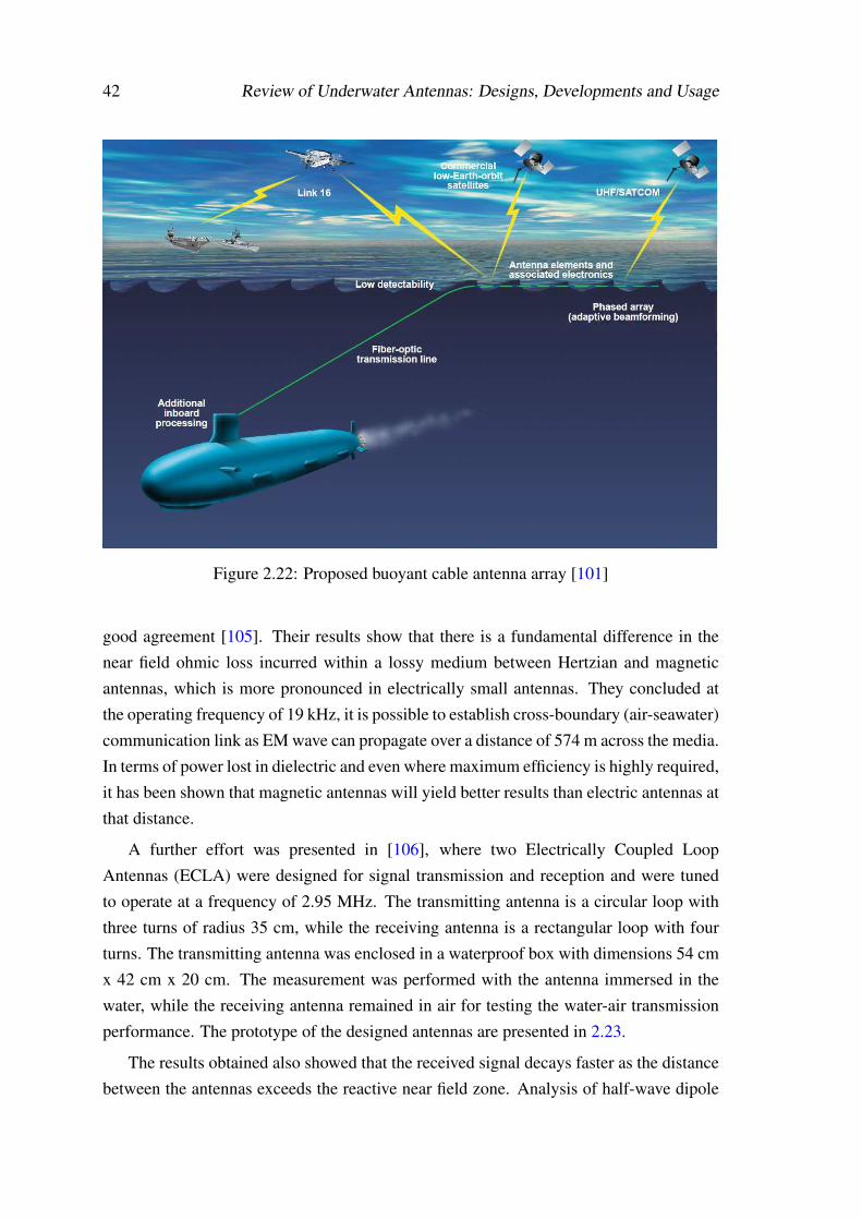
42 Review of Underwater Antennas: Designs, Developments and Usage
Figure 2.22: Proposed buoyant cable antenna array [101]
good agreement [105]. Their results show that there is a fundamental difference in thenear field ohmic loss incurred within a lossy medium between Hertzian and magneticantennas, which is more pronounced in electrically small antennas. They concluded atthe operating frequency of 19 kHz, it is possible to establish cross-boundary (air-seawater)communication link as EM wave can propagate over a distance of 574 m across the media.In terms of power lost in dielectric and even where maximum efficiency is highly required,it has been shown that magnetic antennas will yield better results than electric antennas atthat distance.
A further effort was presented in [106], where two Electrically Coupled LoopAntennas (ECLA) were designed for signal transmission and reception and were tunedto operate at a frequency of 2.95 MHz. The transmitting antenna is a circular loop withthree turns of radius 35 cm, while the receiving antenna is a rectangular loop with fourturns. The transmitting antenna was enclosed in a waterproof box with dimensions 54 cmx 42 cm x 20 cm. The measurement was performed with the antenna immersed in thewater, while the receiving antenna remained in air for testing the water-air transmissionperformance. The prototype of the designed antennas are presented in 2.23.
The results obtained also showed that the received signal decays faster as the distancebetween the antennas exceeds the reactive near field zone. Analysis of half-wave dipole
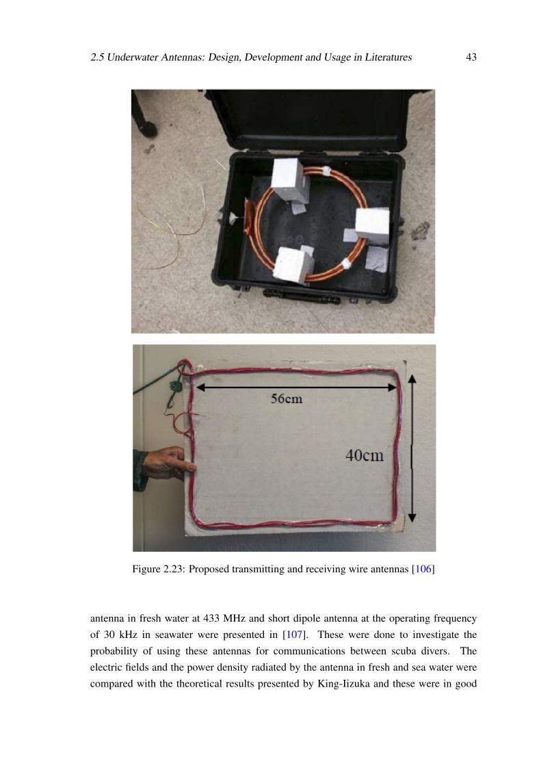
2.5 Underwater Antennas: Design, Development and Usage in Literatures 43
Figure 2.23: Proposed transmitting and receiving wire antennas [106]
antenna in fresh water at 433 MHz and short dipole antenna at the operating frequencyof 30 kHz in seawater were presented in [107]. These were done to investigate theprobability of using these antennas for communications between scuba divers. Theelectric fields and the power density radiated by the antenna in fresh and sea water werecompared with the theoretical results presented by King-Iizuka and these were in good
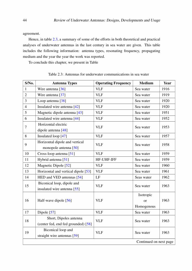
44 Review of Underwater Antennas: Designs, Developments and Usage
agreement.Hence, in table 2.3, a summary of some of the efforts in both theoretical and practical
analyses of underwater antennas in the last century in sea water are given. This tableincludes the following information: antenna types, resonating frequency, propagatingmedium and the year the year the work was reported.
To conclude this chapter, we present in Table
Table 2.3: Antennas for underwater communications in sea water
S/No. Antenna Types Operating Frequency Medium Year1 Wire antenna [36] VLF Sea water 1916
2 Wire antenna [37] VLF Sea water 1919
3 Loop antenna [38] VLF Sea water 1920
4 Insulated wire antenna [42] VLF Sea water 1920
5 Magnetic dipole antenna [43] VLF Sea water 1951
6 Insulated wire antenna [44] VLF Sea water 1952
7Horizontal electricdipole antenna [48]
VLF Sea water 1953
8 Insulated loop [47] VLF Sea water 1957
9Horizontal dipole and vertical
monopole antenna [50]VLF Sea water 1958
10 Cross-loop antenna [51] VLF Sea water 1959
11 Hybrid antenna [51] HF-UHF-IFF Sea water 1959
12 Magnetic Dipole [52] VLF Sea water 1960
13 Horizontal and vertical dipole [53] VLF Sea water 1961
14 HED and VED antennas [54] LF Seas water 1962
15Biconical loop, dipole andinsulated wire antenna [55]
VLF Sea water 1963
16 Half-wave dipole [56] VLFIsotropic
orHomogenous
1963
17 Dipole [57] VLF Sea water 1963
18Short, Dipoles antenna
(center fed, end fed grounded) [58]VLF Sea water 1963
19Biconical loop and
straight wire antennas [59]VLF Sea water 1963
Continued on next page
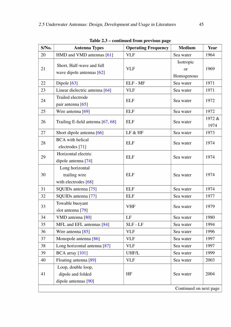
2.5 Underwater Antennas: Design, Development and Usage in Literatures 45
Table 2.3 – continued from previous pageS/No. Antenna Types Operating Frequency Medium Year20 HMD and VMD antennas [61] VLF Sea water 1964
21Short, Half-wave and fullwave dipole antennas [62]
VLFIsotropic
orHomogenous
1969
22 Dipole [63] ELF - MF Sea water 1971
23 Linear dielectric antenna [64] VLF Sea water 1971
24Trailed electrodepair antenna [65]
ELF Sea water 1972
25 Wire antenna [69] ELF Sea water 1972
26 Trailing E-field antenna [67, 68] ELF Sea water1972 &
1974
27 Short dipole antenna [66] LF & HF Sea water 1973
28BCA with helical
electrodes [71]ELF Sea water 1974
29Horizontal electricdipole antenna [74]
ELF Sea water 1974
30Long horizontal
trailing wirewith electrodes [68]
ELF Sea water 1974
31 SQUIDs antenna [75] ELF Sea water 1974
32 SQUIDs antenna [77] ELF Sea water 1977
33Towable buoyantslot antenna [79]
VHF Sea water 1979
34 VMD antenna [80] LF Sea water 1980
35 MFL and EFL antennas [84] SLF - LF Sea water 1994
36 Wire antenna [85] VLF Sea water 1996
37 Monopole antenna [86] VLF Sea water 1997
38 Long horizontal antenna [87] VLF Sea water 1997
39 BCA array [101] UHF/L Sea water 1999
40 Floating antenna [89] VLF Sea water 2003
41Loop, double loop,dipole and folded
dipole antennas [90]
HF Sea water 2004
Continued on next page
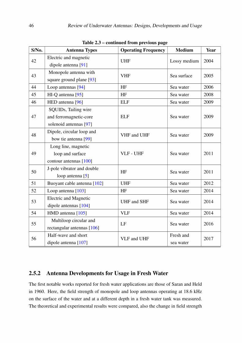
46 Review of Underwater Antennas: Designs, Developments and Usage
Table 2.3 – continued from previous pageS/No. Antenna Types Operating Frequency Medium Year
42Electric and magneticdipole antenna [91]
UHF Lossy medium 2004
43Monopole antenna with
square ground plane [93]VHF Sea surface 2005
44 Loop antennas [94] HF Sea water 2006
45 HI-Q antenna [95] HF Sea water 2008
46 HED antenna [96] ELF Sea water 2009
47SQUIDs, Tailing wire
and ferromagnetic-coresolenoid antennas [97]
ELF Sea water 2009
48Dipole, circular loop and
bow tie antenna [99]VHF and UHF Sea water 2009
49Long line, magnetic
loop and surfacecontour antennas [100]
VLF - UHF Sea water 2011
50J-pole vibrator and double
loop antenna [5]HF Sea water 2011
51 Buoyant cable antenna [102] UHF Sea water 2012
52 Loop antenna [103] HF Sea water 2014
53Electric and Magneticdipole antennas [104]
UHF and SHF Sea water 2014
54 HMD antenna [105] VLF Sea water 2014
55Multiloop circular and
rectangular antennas [106]LF Sea water 2016
56Half-wave and shortdipole antenna [107]
VLF and UHFFresh andsea water
2017
2.5.2 Antenna Developments for Usage in Fresh Water
The first notable works reported for fresh water applications are those of Saran and Heldin 1960. Here, the field strength of monopole and loop antennas operating at 18.6 kHzon the surface of the water and at a different depth in a fresh water tank was measured.The theoretical and experimental results were compared, also the change in field strength
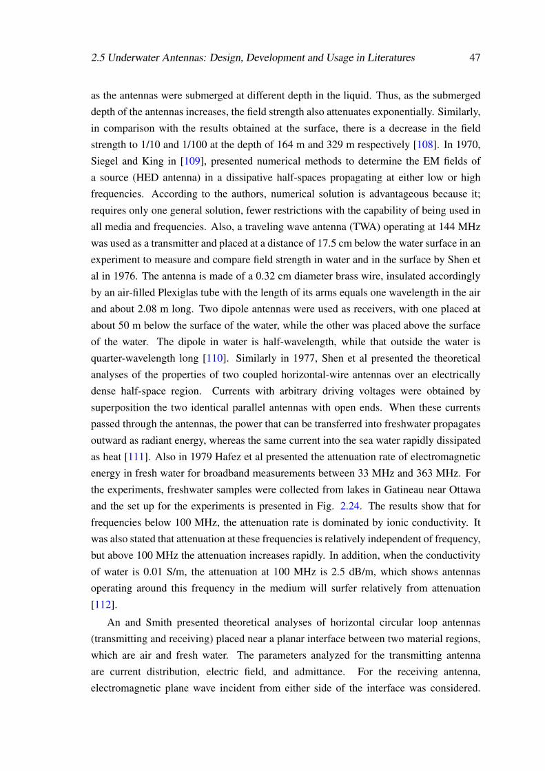
2.5 Underwater Antennas: Design, Development and Usage in Literatures 47
as the antennas were submerged at different depth in the liquid. Thus, as the submergeddepth of the antennas increases, the field strength also attenuates exponentially. Similarly,in comparison with the results obtained at the surface, there is a decrease in the fieldstrength to 1/10 and 1/100 at the depth of 164 m and 329 m respectively [108]. In 1970,Siegel and King in [109], presented numerical methods to determine the EM fields ofa source (HED antenna) in a dissipative half-spaces propagating at either low or highfrequencies. According to the authors, numerical solution is advantageous because it;requires only one general solution, fewer restrictions with the capability of being used inall media and frequencies. Also, a traveling wave antenna (TWA) operating at 144 MHzwas used as a transmitter and placed at a distance of 17.5 cm below the water surface in anexperiment to measure and compare field strength in water and in the surface by Shen etal in 1976. The antenna is made of a 0.32 cm diameter brass wire, insulated accordinglyby an air-filled Plexiglas tube with the length of its arms equals one wavelength in the airand about 2.08 m long. Two dipole antennas were used as receivers, with one placed atabout 50 m below the surface of the water, while the other was placed above the surfaceof the water. The dipole in water is half-wavelength, while that outside the water isquarter-wavelength long [110]. Similarly in 1977, Shen et al presented the theoreticalanalyses of the properties of two coupled horizontal-wire antennas over an electricallydense half-space region. Currents with arbitrary driving voltages were obtained bysuperposition the two identical parallel antennas with open ends. When these currentspassed through the antennas, the power that can be transferred into freshwater propagatesoutward as radiant energy, whereas the same current into the sea water rapidly dissipatedas heat [111]. Also in 1979 Hafez et al presented the attenuation rate of electromagneticenergy in fresh water for broadband measurements between 33 MHz and 363 MHz. Forthe experiments, freshwater samples were collected from lakes in Gatineau near Ottawaand the set up for the experiments is presented in Fig. 2.24. The results show that forfrequencies below 100 MHz, the attenuation rate is dominated by ionic conductivity. Itwas also stated that attenuation at these frequencies is relatively independent of frequency,but above 100 MHz the attenuation increases rapidly. In addition, when the conductivityof water is 0.01 S/m, the attenuation at 100 MHz is 2.5 dB/m, which shows antennasoperating around this frequency in the medium will surfer relatively from attenuation[112].
An and Smith presented theoretical analyses of horizontal circular loop antennas(transmitting and receiving) placed near a planar interface between two material regions,which are air and fresh water. The parameters analyzed for the transmitting antennaare current distribution, electric field, and admittance. For the receiving antenna,electromagnetic plane wave incident from either side of the interface was considered.
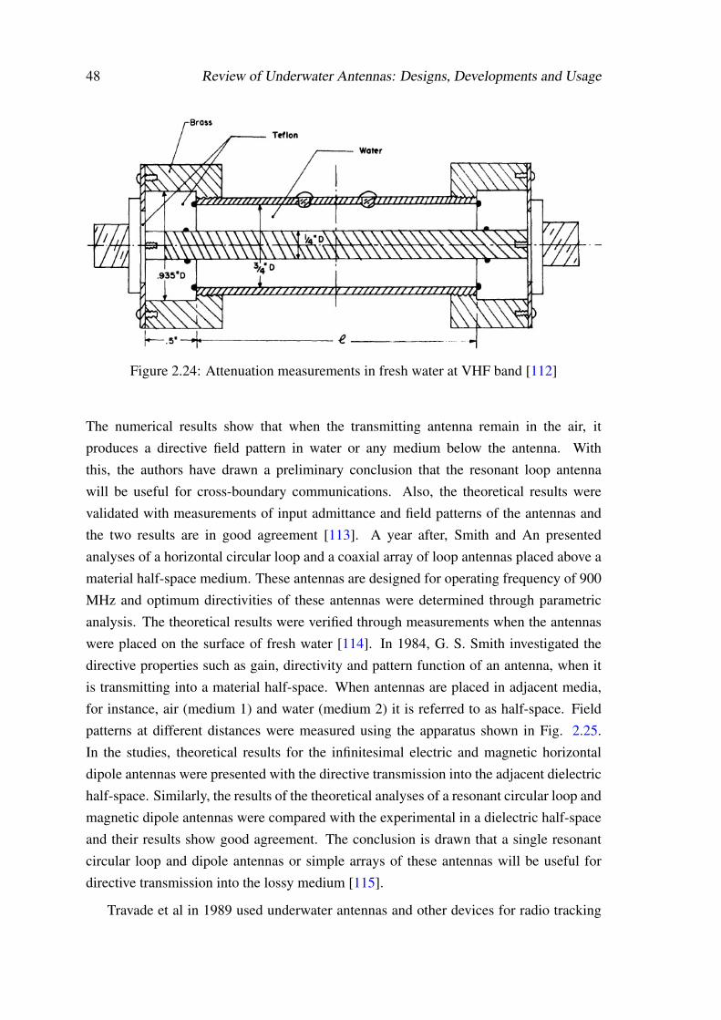
48 Review of Underwater Antennas: Designs, Developments and Usage
Figure 2.24: Attenuation measurements in fresh water at VHF band [112]
The numerical results show that when the transmitting antenna remain in the air, itproduces a directive field pattern in water or any medium below the antenna. Withthis, the authors have drawn a preliminary conclusion that the resonant loop antennawill be useful for cross-boundary communications. Also, the theoretical results werevalidated with measurements of input admittance and field patterns of the antennas andthe two results are in good agreement [113]. A year after, Smith and An presentedanalyses of a horizontal circular loop and a coaxial array of loop antennas placed above amaterial half-space medium. These antennas are designed for operating frequency of 900MHz and optimum directivities of these antennas were determined through parametricanalysis. The theoretical results were verified through measurements when the antennaswere placed on the surface of fresh water [114]. In 1984, G. S. Smith investigated thedirective properties such as gain, directivity and pattern function of an antenna, when itis transmitting into a material half-space. When antennas are placed in adjacent media,for instance, air (medium 1) and water (medium 2) it is referred to as half-space. Fieldpatterns at different distances were measured using the apparatus shown in Fig. 2.25.In the studies, theoretical results for the infinitesimal electric and magnetic horizontaldipole antennas were presented with the directive transmission into the adjacent dielectrichalf-space. Similarly, the results of the theoretical analyses of a resonant circular loop andmagnetic dipole antennas were compared with the experimental in a dielectric half-spaceand their results show good agreement. The conclusion is drawn that a single resonantcircular loop and dipole antennas or simple arrays of these antennas will be useful fordirective transmission into the lossy medium [115].
Travade et al in 1989 used underwater antennas and other devices for radio tracking
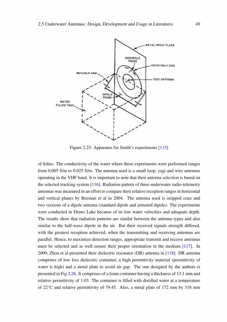
2.5 Underwater Antennas: Design, Development and Usage in Literatures 49
Figure 2.25: Apparatus for Smith’s experiments [115]
of fishes. The conductivity of the water where these experiments were performed rangesfrom 0.005 S/m to 0.025 S/m. The antenna used is a small loop, yagi and wire antennasoperating in the VHF band. It is important to note that their antenna selection is based onthe selected tracking system [116]. Radiation pattern of three underwater radio-telemetryantennas was measured in an effort to compare their relative reception ranges in horizontaland vertical planes by Beeman et al in 2004. The antenna used is stripped coax andtwo versions of a dipole antenna (standard dipole and armored dipole). The experimentswere conducted in Drano Lake because of its low water velocities and adequate depth.The results show that radiation patterns are similar between the antenna types and alsosimilar to the half-wave dipole in the air. But their received signals strength differed,with the greatest reception achieved, when the transmitting and receiving antennas areparallel. Hence, to maximize detection ranges, appropriate transmit and receive antennasmust be selected and as well ensure their proper orientation in the medium [117]. In2009, Zhou et al presented their dielectric resonator (DR) antenna in [118]. DR antennacomprises of low loss dielectric container, a high permittivity material (permittivity ofwater is high) and a metal plate to avoid air gap. The one designed by the authors ispresented in Fig 2.26. It comprises of a foam container having a thickness of 13.1 mm andrelative permittivity of 1.03. The container is filled with distilled water at a temperatureof 22C and relative permittivity of 79.45. Also, a metal plate of 172 mm by 318 mm
50 Review of Underwater Antennas: Designs, Developments and Usage
Figure 2.26: Side view of Dielectric Resonator antenna [118]
is placed on top of the container and an SMA connector is connected through the plate.Though the simulated and the measured reflection coefficient of the DR antenna are ingood agreement, but the antennas were only able to achieve a bandwidth of about 10MHz. Still in the same year, Connesa and Joisel designed an active wideband antennafor underwater tomography. The antenna is a short dipole with a frequency range from100 MHz to 1 GHz [119]. Though this work opens path to new development, when anunderwater antenna is designed for operating frequency above 400 MHz, it suffers fromattenuation greatly.
In [120], three antennas namely dipole, loop and folded dipole operating at 433 MHzwere investigated in a freshwater scenario. This piece of work focuses on measuring thetransmitted and the received power of the antennas with and without insulating materials.The results showed that the performance of the antennas with coating materials performbetter than those without coatings. In 2011, Mendez et al [121] presented a tin-canUHF radio antenna that is compatible with a deep underwater transmission. The centerfrequency of the designed antenna is 2.4 GHz, exhibiting a bandwidth of 100 MHz and areflection coefficient below -10 dB in fresh and sea water. When the surface of the antennawas covered with glass, the bandwidth reduced to 70%, in seawater. The propagationdistance of the antenna recorded in the paper was 200 mm which is too short and willeventually require more of these antenna elements for effective communication. In [122],RF waves propagation in water was investigated for the three ISM bands. The conclusionwas that propagation at 6.7 MHz will yield positive results for a wireless sensor networkfor environmental monitoring. Similarly, in [123] ultrawideband (UWB) bow-tie antennaswere designed for underwater communications. In that work, three modified types of the
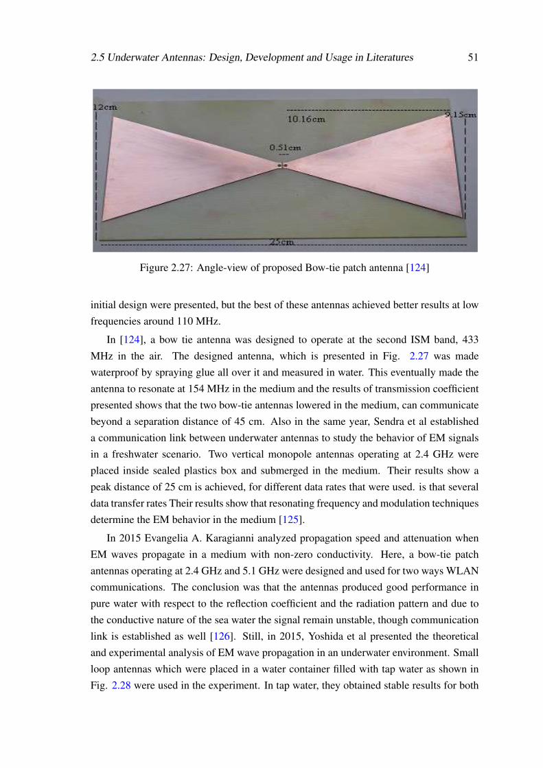
2.5 Underwater Antennas: Design, Development and Usage in Literatures 51
Figure 2.27: Angle-view of proposed Bow-tie patch antenna [124]
initial design were presented, but the best of these antennas achieved better results at lowfrequencies around 110 MHz.
In [124], a bow tie antenna was designed to operate at the second ISM band, 433MHz in the air. The designed antenna, which is presented in Fig. 2.27 was madewaterproof by spraying glue all over it and measured in water. This eventually made theantenna to resonate at 154 MHz in the medium and the results of transmission coefficientpresented shows that the two bow-tie antennas lowered in the medium, can communicatebeyond a separation distance of 45 cm. Also in the same year, Sendra et al establisheda communication link between underwater antennas to study the behavior of EM signalsin a freshwater scenario. Two vertical monopole antennas operating at 2.4 GHz wereplaced inside sealed plastics box and submerged in the medium. Their results show apeak distance of 25 cm is achieved, for different data rates that were used. is that severaldata transfer rates Their results show that resonating frequency and modulation techniquesdetermine the EM behavior in the medium [125].
In 2015 Evangelia A. Karagianni analyzed propagation speed and attenuation whenEM waves propagate in a medium with non-zero conductivity. Here, a bow-tie patchantennas operating at 2.4 GHz and 5.1 GHz were designed and used for two ways WLANcommunications. The conclusion was that the antennas produced good performance inpure water with respect to the reflection coefficient and the radiation pattern and due tothe conductive nature of the sea water the signal remain unstable, though communicationlink is established as well [126]. Still, in 2015, Yoshida et al presented the theoreticaland experimental analysis of EM wave propagation in an underwater environment. Smallloop antennas which were placed in a water container filled with tap water as shown inFig. 2.28 were used in the experiment. In tap water, they obtained stable results for both
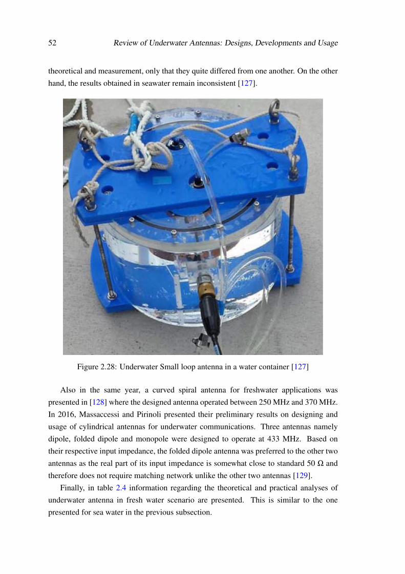
52 Review of Underwater Antennas: Designs, Developments and Usage
theoretical and measurement, only that they quite differed from one another. On the otherhand, the results obtained in seawater remain inconsistent [127].
Figure 2.28: Underwater Small loop antenna in a water container [127]
Also in the same year, a curved spiral antenna for freshwater applications waspresented in [128] where the designed antenna operated between 250 MHz and 370 MHz.In 2016, Massaccessi and Pirinoli presented their preliminary results on designing andusage of cylindrical antennas for underwater communications. Three antennas namelydipole, folded dipole and monopole were designed to operate at 433 MHz. Based ontheir respective input impedance, the folded dipole antenna was preferred to the other twoantennas as the real part of its input impedance is somewhat close to standard 50 Ω andtherefore does not require matching network unlike the other two antennas [129].
Finally, in table 2.4 information regarding the theoretical and practical analyses ofunderwater antenna in fresh water scenario are presented. This is similar to the onepresented for sea water in the previous subsection.
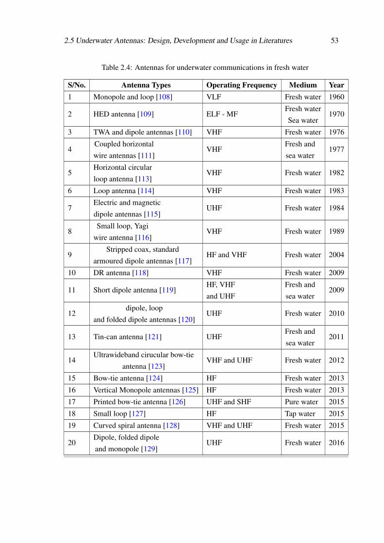
2.5 Underwater Antennas: Design, Development and Usage in Literatures 53
Table 2.4: Antennas for underwater communications in fresh water
S/No. Antenna Types Operating Frequency Medium Year1 Monopole and loop [108] VLF Fresh water 1960
2 HED antenna [109] ELF - MFFresh waterSea water
1970
3 TWA and dipole antennas [110] VHF Fresh water 1976
4Coupled horizontalwire antennas [111]
VHFFresh andsea water
1977
5Horizontal circularloop antenna [113]
VHF Fresh water 1982
6 Loop antenna [114] VHF Fresh water 1983
7Electric and magneticdipole antennas [115]
UHF Fresh water 1984
8Small loop, Yagi
wire antenna [116]VHF Fresh water 1989
9Stripped coax, standard
armoured dipole antennas [117]HF and VHF Fresh water 2004
10 DR antenna [118] VHF Fresh water 2009
11 Short dipole antenna [119]HF, VHFand UHF
Fresh andsea water
2009
12dipole, loop
and folded dipole antennas [120]UHF Fresh water 2010
13 Tin-can antenna [121] UHFFresh andsea water
2011
14Ultrawideband cirucular bow-tie
antenna [123]VHF and UHF Fresh water 2012
15 Bow-tie antenna [124] HF Fresh water 2013
16 Vertical Monopole antennas [125] HF Fresh water 2013
17 Printed bow-tie antenna [126] UHF and SHF Pure water 2015
18 Small loop [127] HF Tap water 2015
19 Curved spiral antenna [128] VHF and UHF Fresh water 2015
20Dipole, folded dipoleand monopole [129]
UHF Fresh water 2016
54 Review of Underwater Antennas: Designs, Developments and Usage
2.6 Conclusion
In this chapter antenna definitions, types and usage in any known media (air, underwater,space) have been duly presented alongside with the three technologies employs in theunderwater environment for operations in the medium. The advantages and disadvantagesof these technologies were also given and it can be said that this research work onlyconsiders the use of electromagnetic waves in underwater environments. Based on this, acomprehensive review of underwater antenna development in the sea and fresh water inthe last 100 years was as well presented. It is therefore important to note that more of theworks published and presented till date have been in the seawater environment, but thisresearch work which will be presented in the later chapters of this thesis are considered inboth fresh and sea water for adequate comparison of propagation in waters with differentconductivities. Lastly, it is important to note that antenna developments for usage in seawater have been considered mainly in the ELF, VLF and LF bands, whereas those of freshwater were considered in the HF, VHF and UHF bands.
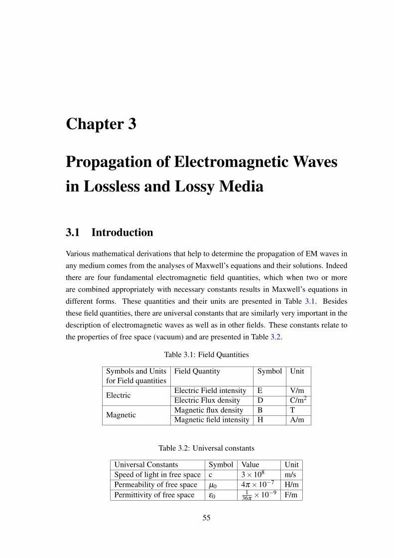
Chapter 3
Propagation of Electromagnetic Wavesin Lossless and Lossy Media
3.1 Introduction
Various mathematical derivations that help to determine the propagation of EM waves inany medium comes from the analyses of Maxwell’s equations and their solutions. Indeedthere are four fundamental electromagnetic field quantities, which when two or moreare combined appropriately with necessary constants results in Maxwell’s equations indifferent forms. These quantities and their units are presented in Table 3.1. Besidesthese field quantities, there are universal constants that are similarly very important in thedescription of electromagnetic waves as well as in other fields. These constants relate tothe properties of free space (vacuum) and are presented in Table 3.2.
Table 3.1: Field Quantities
Symbols and Units Field Quantity Symbol Unitfor Field quantities
ElectricElectric Field intensity E V/mElectric Flux density D C/m2
MagneticMagnetic flux density B TMagnetic field intensity H A/m
Table 3.2: Universal constants
Universal Constants Symbol Value UnitSpeed of light in free space c 3×10⁸ m/sPermeability of free space µ0 4π×10−7 H/mPermittivity of free space ε0
136π×10−9 F/m
55
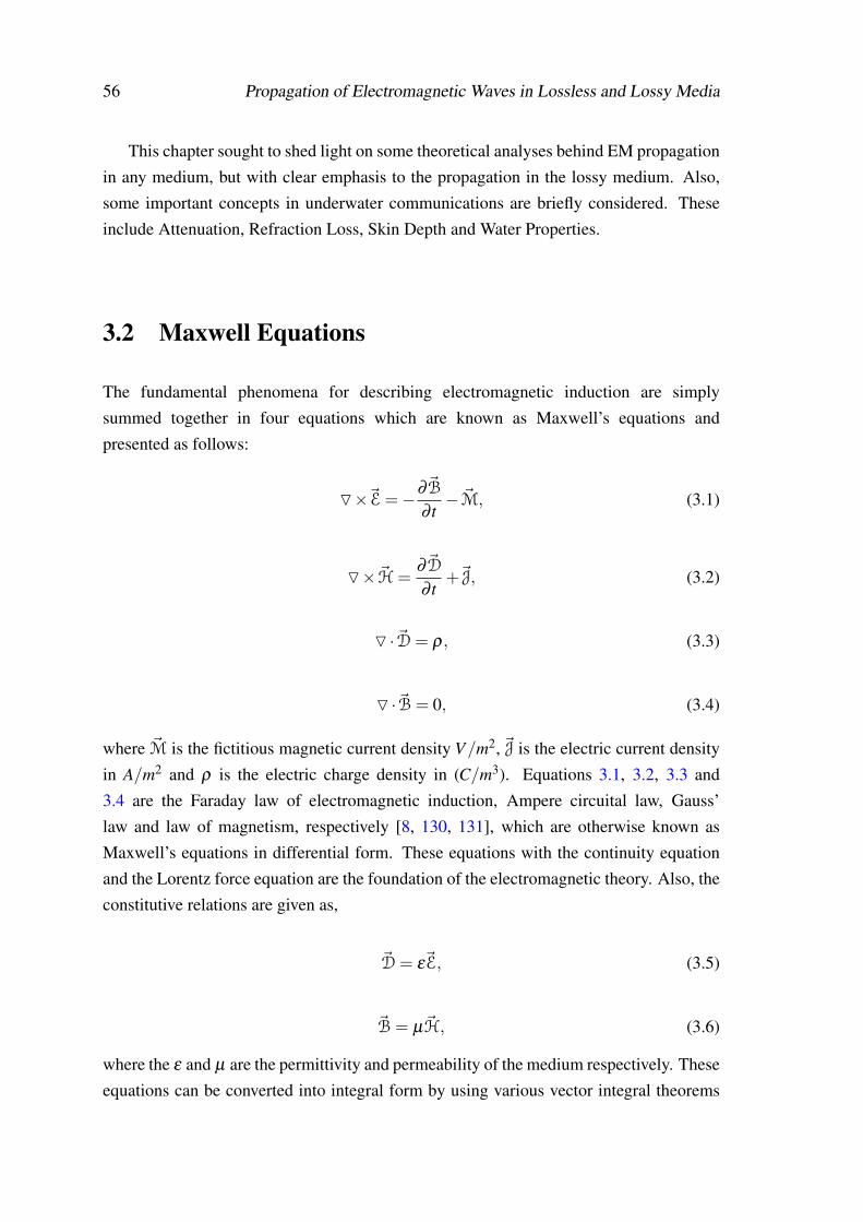
56 Propagation of Electromagnetic Waves in Lossless and Lossy Media
This chapter sought to shed light on some theoretical analyses behind EM propagationin any medium, but with clear emphasis to the propagation in the lossy medium. Also,some important concepts in underwater communications are briefly considered. Theseinclude Attenuation, Refraction Loss, Skin Depth and Water Properties.
3.2 Maxwell Equations
The fundamental phenomena for describing electromagnetic induction are simplysummed together in four equations which are known as Maxwell’s equations andpresented as follows:
O×~E=−∂~B
∂ t− ~M, (3.1)
O× ~H =∂~D
∂ t+~J, (3.2)
O ·~D= ρ, (3.3)
O ·~B= 0, (3.4)
where ~M is the fictitious magnetic current density V/m2, ~J is the electric current densityin A/m2 and ρ is the electric charge density in (C/m3). Equations 3.1, 3.2, 3.3 and3.4 are the Faraday law of electromagnetic induction, Ampere circuital law, Gauss’law and law of magnetism, respectively [8, 130, 131], which are otherwise known asMaxwell’s equations in differential form. These equations with the continuity equationand the Lorentz force equation are the foundation of the electromagnetic theory. Also, theconstitutive relations are given as,
~D= ε~E, (3.5)
~B= µ~H, (3.6)
where the ε and µ are the permittivity and permeability of the medium respectively. Theseequations can be converted into integral form by using various vector integral theorems
3.2 Maxwell Equations 57
yielding:
∮C~E.~dl =− ∂
∂ t
∫S~B.~ds−
∫S~M.~ds, (3.7)
∮C~H.~dl =
∂
∂ t
∫S~D.~ds+
∫S~J.~ds, (3.8)
∫S~B.~ds = 0; (3.9)
∫S~D.~ds =
∫V
ρdv = Q, (3.10)
where Q is the total charge in the close volume V. In a steady state sinusoidal timedependence,~E and ~H will transform as:
~E(x,y,z, t) = E(x,y,z)e jωt , (3.11)
~H(x,y,z, t) = H(x,y,z)e jωt , (3.12)
where ω is the angular frequency in radians/second. Assuming linear and isotropic mediaand taking into consideration an e jωt time dependence, time derivatives in 3.1 to 3.4 canbe replaced by jω . The output of these are Maxwell’s equations in phasor form given as:
O×E =− jωB, (3.13)
O×H = J+ jωD, (3.14)
O ·D =ρ
ε, (3.15)
O ·B = 0. (3.16)
3.2.1 Wave Equations
To solve the problems of wave propagation, the concern is the behavior of an EM wave ina source-free region and also when there are no external current sources, which means ρ
58 Propagation of Electromagnetic Waves in Lossless and Lossy Media
and ~J are both zero. Hence, Maxwell’s curl equations in phasor form are written as:
O×E =− jωµH, (3.17)
O×H = jωεE, (3.18)
O ·E = 0, (3.19)
O ·H = 0. (3.20)
Considering that only equations 3.17 and 3.18 has two unknowns E and H, these can besolved either for one or the other. Thus, further analysis of these equations will involvetaking the curl of these equations and combine them separately for an equation in eachfield. Hence, in the E field the resultant equation is:
O×O×E =− jωµO×H = ω2µεE. (3.21)
Vector identities of the form O×O×P = O(O.P)−O2P was employed to simplify theresult yielding:
O(O.E)−O2E = ω2µεE. (3.22)
Substituting equation 3.19 and rearrange properly 3.22 becomes:
O2E+ω2µεE = 0. (3.23)
Similarly by employing the same mathematical derivatives on the H field componentyield:
O2H+ω2µεH = 0. (3.24)
These two equations, 3.23 and 3.24 are known as Helmholtz equation or wave equationin E and H field respectively.
Further analyses of these equations yield the velocity of propagation of the wave in themedium which is 1√
µε. But:
µ = µ0µr, (3.25)
andε = ε0εr, (3.26)
3.2 Maxwell Equations 59
where µ0 and ε0 and the magnetic permeability and electrical permittivity of free spacedefined among the universal constants given in Table 3.2. Also µr εr are the relativemagnetic permeability and electrical permittivity of the medium. In free space, µr = εr =1and the resultant parameter is the third element among the universal constant, which is thespeed of light. The propagation constant or wave number is another important parameterthat can be derived from 3.23 and 3.24, and is defined as k = ω
√µε .
Thus, the two equations are re-written as:
O2E+ k2E = 0. (3.27)
O2H+ k2H = 0. (3.28)
Hence, by squaring this propagation constant, the resulting element satisfies thecomponent of ~E in equation 3.23.
3.2.2 Plane Waves in Lossless (Non-Conducting) Media
If the wave equation in 3.23 is considered in Cartesian coordinate, it will yield three scalarHelmholtz’s equation, Ex, Ey and Ez and these components are written for Ex directiononly we have:
(∂ 2
∂x2 +∂ 2
∂y2 +∂ 2
∂ z2 + k20
)Ex = 0. (3.29)
Thus, for an electric field with only x component and no variation in x and y, then ∂E∂x
= ∂E∂y =0, then wave equation reduces to:
∂ 2Ex
∂ z2 + k20Ex = 0, (3.30)
equation 3.30 is an ordinary differential equation, where Ex depends only on z. Thus,solution to this equation can be readily obtained in the form:
Ex (z) = E+e− jkz +E−e− jkz, (3.31)
where E+ and E− are arbitrary constant values representing the amplitudes of the forwardand backward propagating waves, respectively. Also when equation 3.23 is applied to the
60 Propagation of Electromagnetic Waves in Lossless and Lossy Media
electric field in the last equation, the resultant solution is the magnetic field counterpart:
Hx (z) = 0, (3.32)
Hz (z) = 0, (3.33)
Hy (z) =1η
[E+e− jkz−E−e− jkz
], (3.34)
where η is the wave impedance, which can be expressed as η = ωµ/k =√
µ/ε and isknown as ratio of E and H fields. In planes waves, the wave impedance is equal to theintrinsic impedance. Thus, in free-space, the intrinsic impedance η0 =
√µ0/ε0 = 377Ω.
Full mathematical analysis of this derivation is not covered here, but can be found in[8, 132, 130]
3.2.3 Plane Waves in Lossy (Conducting) Media
This aspect is very important in this work because further research reported is practicallybased on wave propagation in this environment. The derivation for plane waves in alossless medium can be modified to apply to wave propagation in a lossy medium. Thisis achieved by replacing k in equation 3.27 with kc and the equation becomes:
O2E+ k2cE = 0. (3.35)
In this case kc is a complex quantity, defined as:
kc = ω√
µεc, (3.36)
where εc is a complex electrical permittivity.
Based on the analysis presented in the Cole-Cole equation [133, 134] and Debye model[3, 135], complex permittivity in a conductive medium has been described mathematically[136] and can be presented as:
εc = ε− jσ
ω= F/m, (3.37)
where σ is the conductivity measured in Siemens per meter, j is the imaginary unit(=√−1), and ε is already defined in 3.26.
3.2 Maxwell Equations 61
This equation can be further expressed in line with Debye model, such that thecomplex relative permittivity is dependent on factors like frequency, temperature, andsalinity. This is presented as:
εc = ε0
ε∞ +
εs− ε∞
1+(
j ffrel
)− jσ
ω, (3.38)
where εs and ε∞ are the real part of the relative permittivity at low and high frequenciesrespectively, frel is the relaxation frequency and f is the operating frequency measured inHertz.
Based on equation 3.37, equation 3.35 is re-written as:
O2E+ω2µε(1− j
σ
ωε)E = 0 (3.39)
and the conjugate in H plane is written as:
O2H+ω2µε(1− j
σ
ωε)H = 0 (3.40)
But the complex propagation constant, γ , can be written as:
γ = jkc = jω√
µεc, (3.41)
which is the same component ω2µε(1− j σ
ωε) in equation 3.39 and 3.40, and be can
re-arranged as [3, 137] √jωµ( jωε +σ) = α + jβ , (3.42)
where α and β are respectively the real and the imaginary parts of γ and are also knownas the attenuation constant in Neper per meter and the phase constant in radians per unitlength respectively.
62 Propagation of Electromagnetic Waves in Lossless and Lossy Media
3.3 Impairments of Lossy Media on Wave Propagation
3.3.1 Water properties
In [8] the author classified propagating media into two different types which are: dielectricand conducting media. A medium is referred to as a dielectric or insulator lossy mediumif σ /ωε «1. This means that the displacement current is much greater than the conductivecurrent. Conversely, when σ /ωε »1, the media is considered to be a good conductor,meaning the conductive current is much greater than the displacement current. It is basedon these analyses that the dependence of σ /ωε as a function of operating frequency forfresh and sea water is presented in Fig. 3.1, which was obtained from the previousanalysis, specifically from equation 3.37. From the plots, the horizontal line indicatesthe medium where σ /ωε = 1, but also serves as a demarcation between the conductingmedium (region above the line) and the dielectric medium (the region below the line). Itcan also be seen that for frequencies below 10 MHz, freshwater behaves as a conductor,it thereafter behaves as a dielectric medium, whereas the change from conducting todielectric occurs at 888 MHz in seawater [138]. This simply means it is only at lowerfrequencies that sea water behaves as a good conductor. Thus, the frequency at whichfresh and seawater change from conducting to dielectric medium is known as transitionfrequency.
3.3.2 Attenuation
Attenuation in relation to underwater technology is defined as a gradual loss of signalintensity which is the resultant effect of scattering from the water, dissolved impurities(including organic and inorganic substance) and the intrinsic absorption by water [140].Thus, it is important to note the full breakdown of the expression in the right hand sideof equation 3.42 for α and β are given as equation 3.43 and 3.44 respectively [3], whichare:
α = ω√
µε
√√√√12
(√1+(
σ
ωε
)2−1
)(3.43)
β = ω√
µε
√√√√12
(√1+(
σ
ωε
)2+1
)(3.44)
where α is the attenuation coefficient and β the propagation constant. These twoequations are vital for understanding the attenuation at various operating frequencies,which will be used in determining the best operating frequency of the underwater
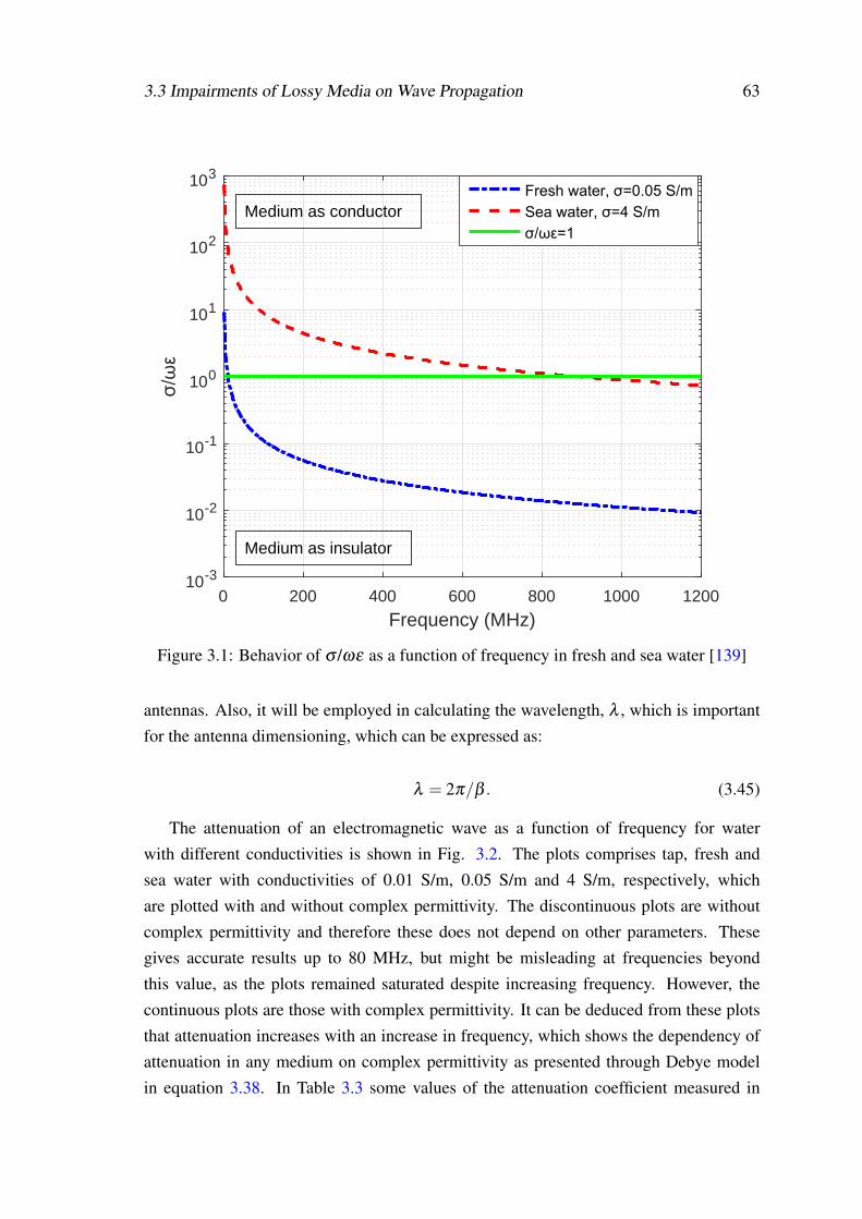
3.3 Impairments of Lossy Media on Wave Propagation 63
0 200 400 600 800 1000 1200
Frequency (MHz)
10-3
10-2
10-1
100
101
102
103
Medium as insulator
Medium as conductor
Figure 3.1: Behavior of σ /ωε as a function of frequency in fresh and sea water [139]
antennas. Also, it will be employed in calculating the wavelength, λ , which is importantfor the antenna dimensioning, which can be expressed as:
λ = 2π/β . (3.45)
The attenuation of an electromagnetic wave as a function of frequency for waterwith different conductivities is shown in Fig. 3.2. The plots comprises tap, fresh andsea water with conductivities of 0.01 S/m, 0.05 S/m and 4 S/m, respectively, whichare plotted with and without complex permittivity. The discontinuous plots are withoutcomplex permittivity and therefore these does not depend on other parameters. Thesegives accurate results up to 80 MHz, but might be misleading at frequencies beyondthis value, as the plots remained saturated despite increasing frequency. However, thecontinuous plots are those with complex permittivity. It can be deduced from these plotsthat attenuation increases with an increase in frequency, which shows the dependency ofattenuation in any medium on complex permittivity as presented through Debye modelin equation 3.38. In Table 3.3 some values of the attenuation coefficient measured in
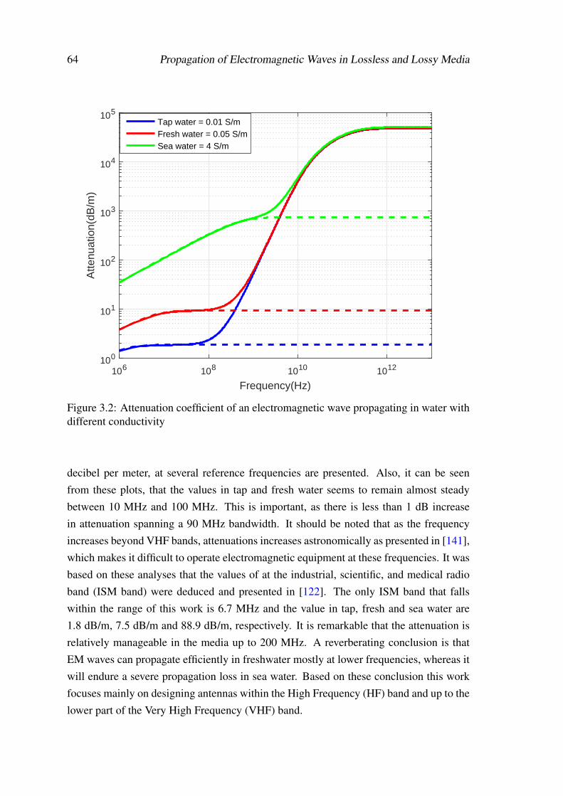
64 Propagation of Electromagnetic Waves in Lossless and Lossy Media
106 108 1010 1012
Frequency(Hz)
100
101
102
103
104
105
Atte
nuat
ion(
dB/m
)
Tap water = 0.01 S/mFresh water = 0.05 S/mSea water = 4 S/m
Figure 3.2: Attenuation coefficient of an electromagnetic wave propagating in water withdifferent conductivity
decibel per meter, at several reference frequencies are presented. Also, it can be seenfrom these plots, that the values in tap and fresh water seems to remain almost steadybetween 10 MHz and 100 MHz. This is important, as there is less than 1 dB increasein attenuation spanning a 90 MHz bandwidth. It should be noted that as the frequencyincreases beyond VHF bands, attenuations increases astronomically as presented in [141],which makes it difficult to operate electromagnetic equipment at these frequencies. It wasbased on these analyses that the values of at the industrial, scientific, and medical radioband (ISM band) were deduced and presented in [122]. The only ISM band that fallswithin the range of this work is 6.7 MHz and the value in tap, fresh and sea water are1.8 dB/m, 7.5 dB/m and 88.9 dB/m, respectively. It is remarkable that the attenuation isrelatively manageable in the media up to 200 MHz. A reverberating conclusion is thatEM waves can propagate efficiently in freshwater mostly at lower frequencies, whereas itwill endure a severe propagation loss in sea water. Based on these conclusion this workfocuses mainly on designing antennas within the High Frequency (HF) band and up to thelower part of the Very High Frequency (VHF) band.
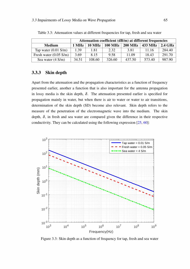
3.3 Impairments of Lossy Media on Wave Propagation 65
Table 3.3: Attenuation values at different frequencies for tap, fresh and sea water
Attenuation coefficient (dB/m) at different frequenciesMedium 1 MHz 10 MHz 100 MHz 200 MHz 433 MHz 2.4 GHz
Tap water (0.01 S/m) 1.39 1.81 2.32 3.81 11.16 284.40Fresh water (0.05 S/m) 3.69 8.15 9.58 11.09 18.43 291.70
Sea water (4 S/m) 34.51 108.60 326.60 437.50 573.40 987.90
3.3.3 Skin depth
Apart from the attenuation and the propagation characteristics as a function of frequencypresented earlier, another a function that is also important for the antenna propagationin lossy media is the skin depth, δ . The attenuation presented earlier is specified forpropagation mainly in water, but when there is air to water or water to air transitions,determination of the skin depth (SD) become also relevant. Skin depth refers to themeasure of the penetration of the electromagnetic wave into the medium. The skindepth, δ , in fresh and sea water are compared given the difference in their respectiveconductivity. They can be calculated using the following expression [25, 60]:
103 104 105 106 107 108 109
Frequency(Hz)
10-3
10-2
10-1
100
101
102
103
Ski
n de
pth
(mm
)
Tap water = 0.01 S/mFresh water = 0.05 S/mSea water = 4 S/m
Figure 3.3: Skin depth as a function of frequency for tap, fresh and sea water
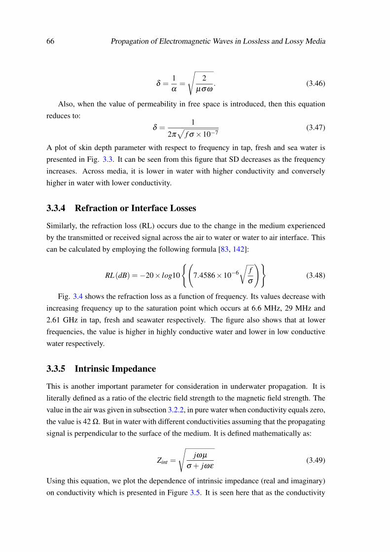
66 Propagation of Electromagnetic Waves in Lossless and Lossy Media
δ =1α
=
√2
µσω. (3.46)
Also, when the value of permeability in free space is introduced, then this equationreduces to:
δ =1
2π√
f σ ×10−7(3.47)
A plot of skin depth parameter with respect to frequency in tap, fresh and sea water ispresented in Fig. 3.3. It can be seen from this figure that SD decreases as the frequencyincreases. Across media, it is lower in water with higher conductivity and converselyhigher in water with lower conductivity.
3.3.4 Refraction or Interface Losses
Similarly, the refraction loss (RL) occurs due to the change in the medium experiencedby the transmitted or received signal across the air to water or water to air interface. Thiscan be calculated by employing the following formula [83, 142]:
RL(dB) =−20× log10
(7.4586×10⁻⁶
√fσ
)(3.48)
Fig. 3.4 shows the refraction loss as a function of frequency. Its values decrease withincreasing frequency up to the saturation point which occurs at 6.6 MHz, 29 MHz and2.61 GHz in tap, fresh and seawater respectively. The figure also shows that at lowerfrequencies, the value is higher in highly conductive water and lower in low conductivewater respectively.
3.3.5 Intrinsic Impedance
This is another important parameter for consideration in underwater propagation. It isliterally defined as a ratio of the electric field strength to the magnetic field strength. Thevalue in the air was given in subsection 3.2.2, in pure water when conductivity equals zero,the value is 42 Ω. But in water with different conductivities assuming that the propagatingsignal is perpendicular to the surface of the medium. It is defined mathematically as:
Zint =
√jωµ
σ + jωε(3.49)
Using this equation, we plot the dependence of intrinsic impedance (real and imaginary)on conductivity which is presented in Figure 3.5. It is seen here that as the conductivity
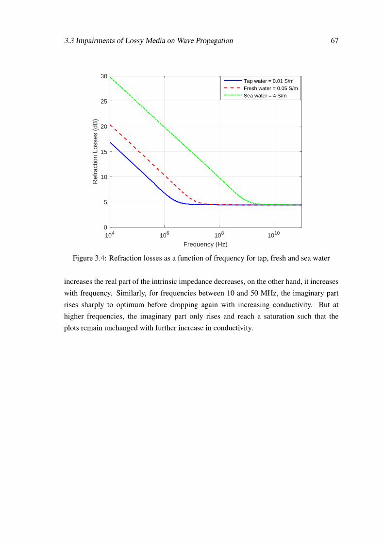
3.3 Impairments of Lossy Media on Wave Propagation 67
104 106 108 1010
Frequency (Hz)
0
5
10
15
20
25
30
Ref
ract
ion
Loss
es (
dB)
Tap water = 0.01 S/mFresh water = 0.05 S/mSea water = 4 S/m
Figure 3.4: Refraction losses as a function of frequency for tap, fresh and sea water
increases the real part of the intrinsic impedance decreases, on the other hand, it increaseswith frequency. Similarly, for frequencies between 10 and 50 MHz, the imaginary partrises sharply to optimum before dropping again with increasing conductivity. But athigher frequencies, the imaginary part only rises and reach a saturation such that theplots remain unchanged with further increase in conductivity.
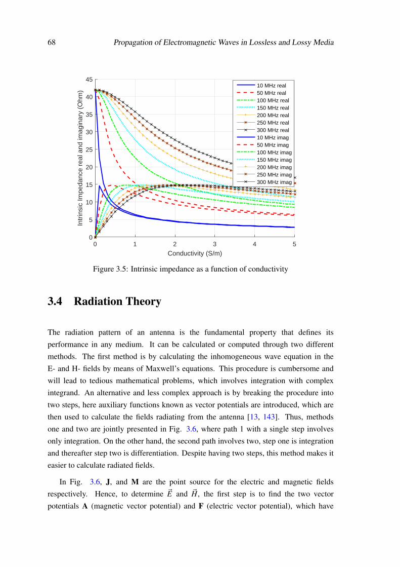
68 Propagation of Electromagnetic Waves in Lossless and Lossy Media
0 1 2 3 4 5
Conductivity (S/m)
0
5
10
15
20
25
30
35
40
45In
trin
sic
Impe
danc
e re
al a
nd im
agin
ary
(Ohm
)10 MHz real50 MHz real100 MHz real150 MHz real200 MHz real250 MHz real300 MHz real10 MHz imag50 MHz imag100 MHz imag150 MHz imag200 MHz imag250 MHz imag300 MHz imag
Figure 3.5: Intrinsic impedance as a function of conductivity
3.4 Radiation Theory
The radiation pattern of an antenna is the fundamental property that defines itsperformance in any medium. It can be calculated or computed through two differentmethods. The first method is by calculating the inhomogeneous wave equation in theE- and H- fields by means of Maxwell’s equations. This procedure is cumbersome andwill lead to tedious mathematical problems, which involves integration with complexintegrand. An alternative and less complex approach is by breaking the procedure intotwo steps, here auxiliary functions known as vector potentials are introduced, which arethen used to calculate the fields radiating from the antenna [13, 143]. Thus, methodsone and two are jointly presented in Fig. 3.6, where path 1 with a single step involvesonly integration. On the other hand, the second path involves two, step one is integrationand thereafter step two is differentiation. Despite having two steps, this method makes iteasier to calculate radiated fields.
In Fig. 3.6, J, and M are the point source for the electric and magnetic fieldsrespectively. Hence, to determine ~E and ~H, the first step is to find the two vectorpotentials A (magnetic vector potential) and F (electric vector potential), which have
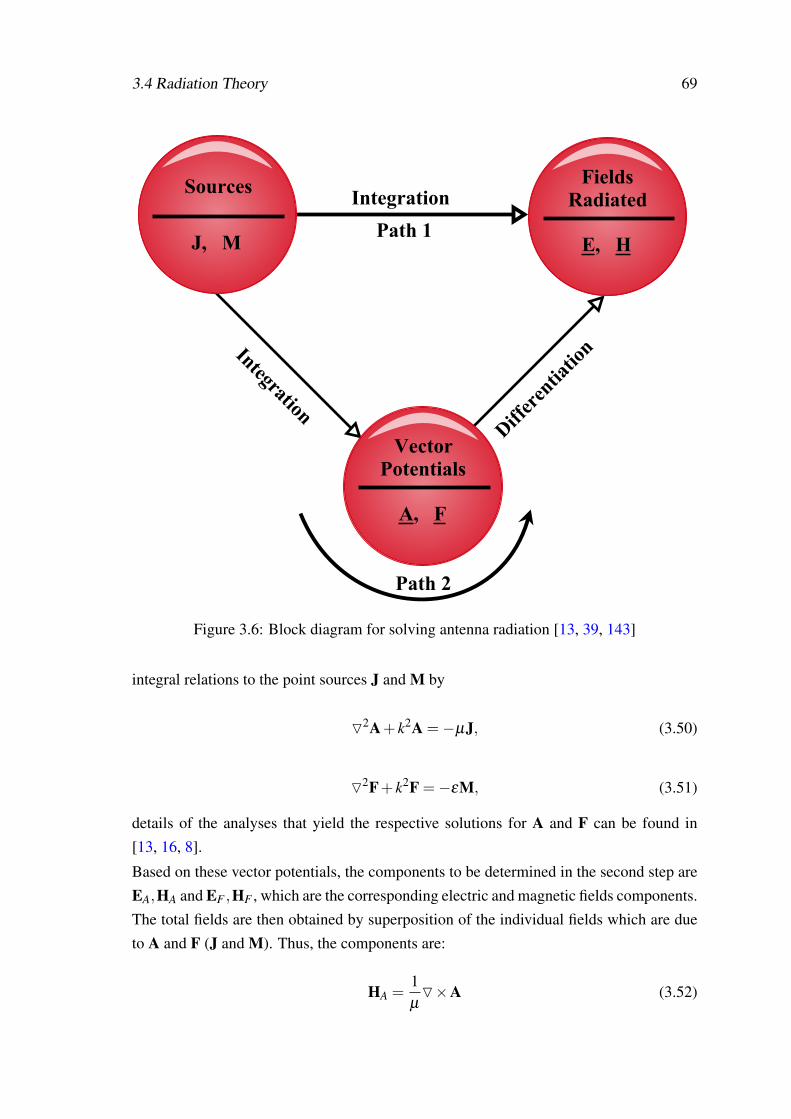
3.4 Radiation Theory 69
Vector Potentials
A, F
Fields Radiated
E, H
Sources
J, M
Integration
Path 1
Integration
Differ
entia
tion
Path 2
Figure 3.6: Block diagram for solving antenna radiation [13, 39, 143]
integral relations to the point sources J and M by
O2A+ k2A =−µJ, (3.50)
O2F+ k2F =−εM, (3.51)
details of the analyses that yield the respective solutions for A and F can be found in[13, 16, 8].
Based on these vector potentials, the components to be determined in the second step areEA,HA and EF ,HF , which are the corresponding electric and magnetic fields components.The total fields are then obtained by superposition of the individual fields which are dueto A and F (J and M). Thus, the components are:
HA =1µO×A (3.52)
70 Propagation of Electromagnetic Waves in Lossless and Lossy Media
EA =− jωA− j1
ωµεO(O.A) (3.53)
EF =−1εO×F (3.54)
HF =− jωF− jωµε
O(O.F) (3.55)
In summary, the following steps are employed to determine the fields components fromthe point sources through the vector potentials:
• Specify the sources for the electric current density, J and the magnetic currentdensity, M respectively;
• Using the Integral method, determine A (due to J) and F (due to M);
• and then the differential method to find HA and EA as well as EF and HF ;
• Finally determines the total fields which are the sum of the electric and magneticcomponents.
When current densities are distributed over a thin wire of a very short length as shown inFig. 3.7, the line integral of the vector potentials of 3.50 and 3.51 are presented as:
A =µ
4π
∫C
Ie
(x′,y′,z′)
e− jkR
R dl′, (3.56)
F =ε
4π
∫C
Im
(x′,y′,z′)
e− jkR
R dl′, (3.57)
but if the wire carries only electric current Ie, it means the magnetic current Im equalsto zero thereby, the vector potential F also equal to zero, the vector potential A, whichoriented from the source along the z axis such that Ie
(z′)= azIe is presented as:
A =µ
4π
∫C
azIee− jkR
R dl′, (3.58)
these equations in phasor form can be presented as:
A = azµ0Idl
4π
(e− jkR
R
)(3.59)
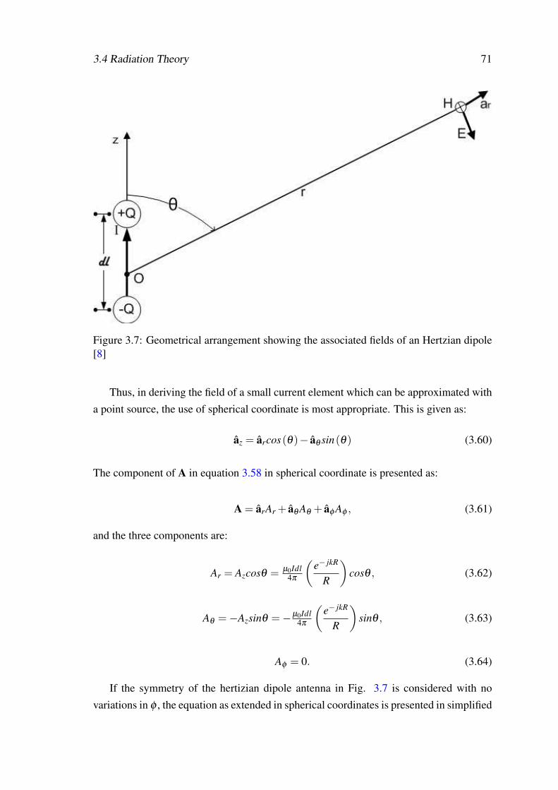
3.4 Radiation Theory 71
Figure 3.7: Geometrical arrangement showing the associated fields of an Hertzian dipole[8]
Thus, in deriving the field of a small current element which can be approximated witha point source, the use of spherical coordinate is most appropriate. This is given as:
az = arcos(θ)− aθ sin(θ) (3.60)
The component of A in equation 3.58 in spherical coordinate is presented as:
A = arAr + aθ Aθ + aφ Aφ , (3.61)
and the three components are:
Ar = Azcosθ = µ0Idl4π
(e− jkR
R
)cosθ , (3.62)
Aθ =−Azsinθ =−µ0Idl4π
(e− jkR
R
)sinθ , (3.63)
Aφ = 0. (3.64)
If the symmetry of the hertizian dipole antenna in Fig. 3.7 is considered with novariations in φ , the equation as extended in spherical coordinates is presented in simplified
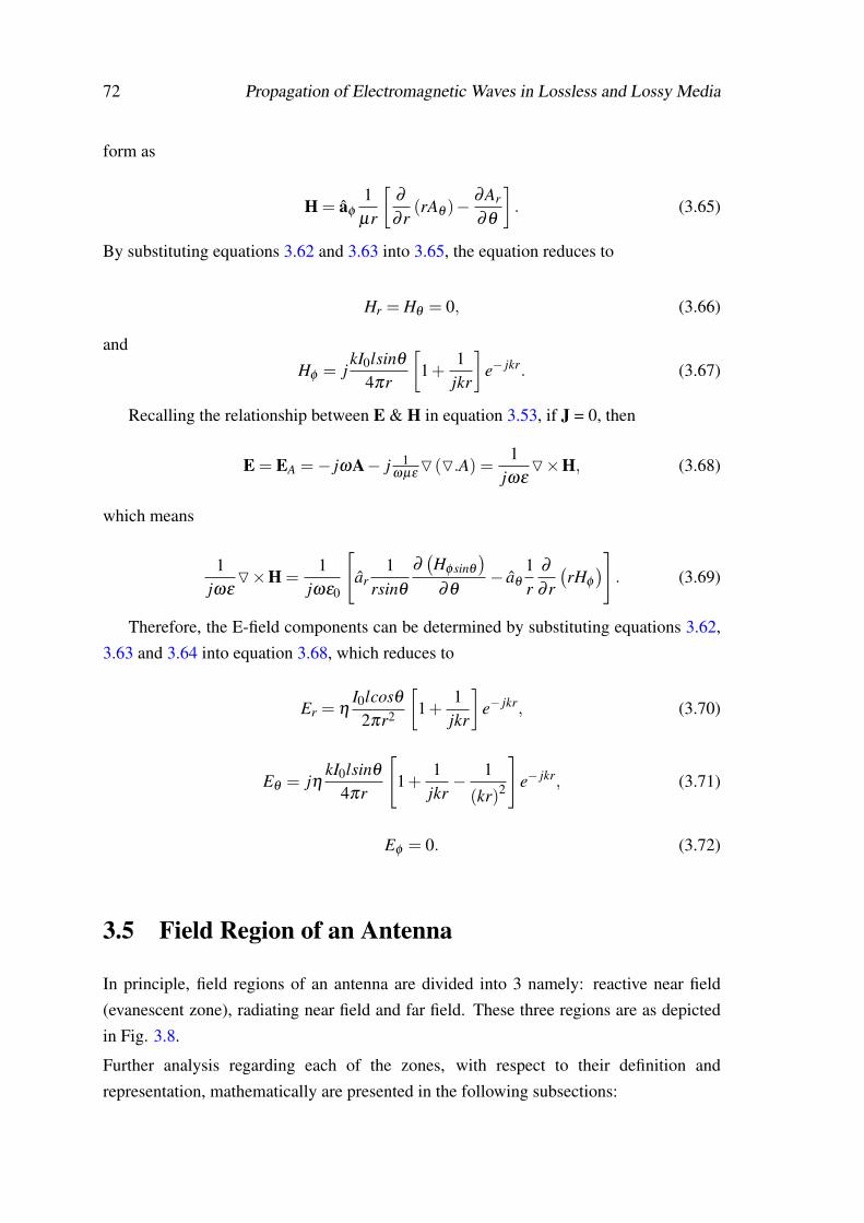
72 Propagation of Electromagnetic Waves in Lossless and Lossy Media
form as
H = aφ
1µr
[∂
∂ r(rAθ )−
∂Ar
∂θ
]. (3.65)
By substituting equations 3.62 and 3.63 into 3.65, the equation reduces to
Hr = Hθ = 0, (3.66)
andHφ = j
kI0lsinθ
4πr
[1+
1jkr
]e− jkr. (3.67)
Recalling the relationship between E & H in equation 3.53, if J = 0, then
E = EA =− jωA− j 1ωµε
O(O.A) =1
jωεO×H, (3.68)
which means
1jωε
O×H =1
jωε0
[ar
1rsinθ
∂(Hφsinθ
)∂θ
− aθ
1r
∂
∂ r
(rHφ
)]. (3.69)
Therefore, the E-field components can be determined by substituting equations 3.62,3.63 and 3.64 into equation 3.68, which reduces to
Er = ηI0lcosθ
2πr2
[1+
1jkr
]e− jkr, (3.70)
Eθ = jηkI0lsinθ
4πr
[1+
1jkr− 1
(kr)2
]e− jkr, (3.71)
Eφ = 0. (3.72)
3.5 Field Region of an Antenna
In principle, field regions of an antenna are divided into 3 namely: reactive near field(evanescent zone), radiating near field and far field. These three regions are as depictedin Fig. 3.8.
Further analysis regarding each of the zones, with respect to their definition andrepresentation, mathematically are presented in the following subsections:
3.5 Field Region of an Antenna 73
Figure 3.8: Antenna’s Field Regions [13, 143]
3.5.1 Reactive Near Fields
This is the immediate area/environment of an antenna. The region is dominated byreactive fields. In other words, it means E-field and H-field are out of phase by 90 toeach other. Mathematically, the boundary of the region is given as:
0.62
√l3
λ> r > 0, (3.73)
where l is the length of a wire antenna which is equivalent to the largest dimension of theantenna, D. To present this in spherical coordinates, the conditions that must be satisfiedare kr << 1 and when kr << λ or r << λ/2π , the components of E-field and H-field
74 Propagation of Electromagnetic Waves in Lossless and Lossy Media
are:
Er =− jηI0le− jkr
2πkr3 cosθ , (3.74)
Eθ =− jηI0le− jkr
4πkr3 sinθ , (3.75)
Eφ = Hr = Hθ = 0, (3.76)
Hφ =I0le− jkr
4πr2 sinθ . (3.77)
3.5.2 Radiative Near Fields or Fresnel Region
This is the region sandwiched between the reactive near-field and the far-field. Here theradiation fields predominate and the angular field distribution depends largely upon thedistance from the antenna. But in the case of antennas where D « λ the region may notexist. Thus, radiative near field region is presented as
2l2
λ> r > 0.62
√l3
λ(3.78)
This region is also called intermediate region, where the values of kr begin to increase andgreater than unity. It is often called Fresnel region and the radiating near field parameterswhere kr > 1 can be presented in spherical coordinates as:
Er = ηI0le− jkr
2πkr2 cosθ , (3.79)
Eθ = jηkI0le− jkr
4πrsinθ , (3.80)
Eφ = Hr = Hθ = 0, (3.81)
Hφ =kI0le− jkr
4πrsinθ . (3.82)
3.5.3 Farfields or Fraunhofer Region
This is the region that is farthest away from the antenna where the angular fielddistribution does not depend on the distance from the antenna (propagating waves). Hencethe region is given mathematically as:
∞ > r >2l2
λ(3.83)
In this region, kr >> 1 and also r > λ . Hence, Er is inversely proportional to r2 and willbe smaller than Eθ . Similarly, Eθ is inversely proportional to r and their field components
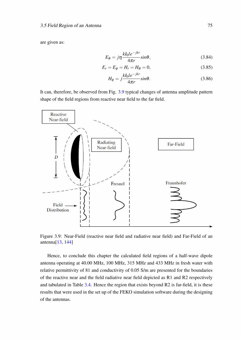
3.5 Field Region of an Antenna 75
are given as:
Eθ = jηkI0le− jkr
4πrsinθ , (3.84)
Er = Eφ = Hr = Hθ = 0, (3.85)
Hφ = jkI0le− jkr
4πrsinθ . (3.86)
It can, therefore, be observed from Fig. 3.9 typical changes of antenna amplitude patternshape of the field regions from reactive near field to the far field.
Figure 3.9: Near-Field (reactive near field and radiative near field) and Far-Field of anantenna[13, 144]
Hence, to conclude this chapter the calculated field regions of a half-wave dipoleantenna operating at 40.00 MHz, 100 MHz, 315 MHz and 433 MHz in fresh water withrelative permittivity of 81 and conductivity of 0.05 S/m are presented for the boundariesof the reactive near and the field radiative near field depicted as R1 and R2 respectivelyand tabulated in Table 3.4. Hence the region that exists beyond R2 is far-field, it is theseresults that were used in the set up of the FEKO simulation software during the designingof the antennas.
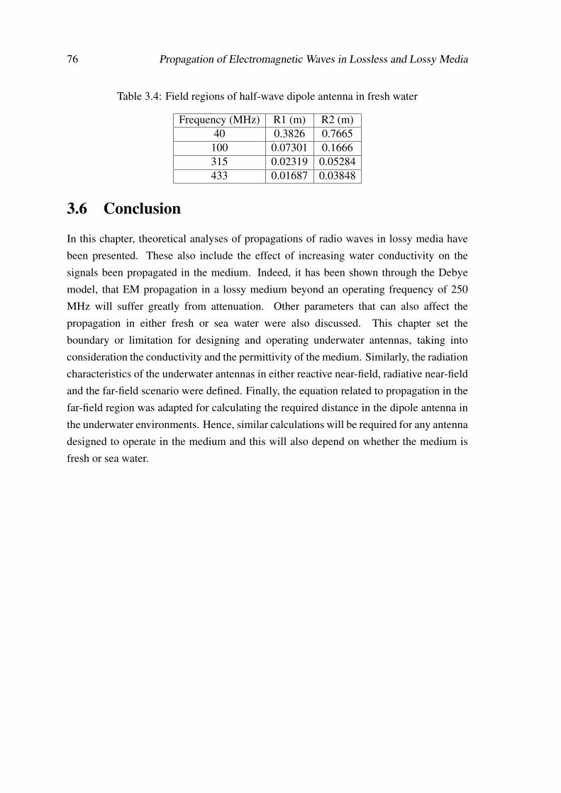
76 Propagation of Electromagnetic Waves in Lossless and Lossy Media
Table 3.4: Field regions of half-wave dipole antenna in fresh water
Frequency (MHz) R1 (m) R2 (m)40 0.3826 0.7665
100 0.07301 0.1666315 0.02319 0.05284433 0.01687 0.03848
3.6 Conclusion
In this chapter, theoretical analyses of propagations of radio waves in lossy media havebeen presented. These also include the effect of increasing water conductivity on thesignals been propagated in the medium. Indeed, it has been shown through the Debyemodel, that EM propagation in a lossy medium beyond an operating frequency of 250MHz will suffer greatly from attenuation. Other parameters that can also affect thepropagation in either fresh or sea water were also discussed. This chapter set theboundary or limitation for designing and operating underwater antennas, taking intoconsideration the conductivity and the permittivity of the medium. Similarly, the radiationcharacteristics of the underwater antennas in either reactive near-field, radiative near-fieldand the far-field scenario were defined. Finally, the equation related to propagation in thefar-field region was adapted for calculating the required distance in the dipole antenna inthe underwater environments. Hence, similar calculations will be required for any antennadesigned to operate in the medium and this will also depend on whether the medium isfresh or sea water.
Chapter 4
Design and Analyses of Narrow bandUnderwater Antennas
4.1 Introduction
This chapter can be summarily divided into two sections, while the first part focuseson full analyses of underwater antennas with respect to the type of materials, changein conductivity, the coating of the wires, as well as when the antennas are placed in anair-filled casing. The second part is about design, construction, and testing of some namednarrowband antennas that can be deployed with an AUV for data harvesting and alsoguiding the AUV to a docking station for recharging through wireless power transfer.These antennas are accessed in terms of their achievable bandwidth and directivity whenthey are submerged in both fresh and sea water. It is worth noting that these are narrowband antennas with bandwidth not exceeding 40 MHz.
4.2 Simulation Software
There are many simulation software used for antenna design and analysis. Thetop five are; High-Frequency Structure Simulator (HFSS), FEKO (it is acronym ofGerman words translated into English as "field calculations involving bodies of arbitraryshape"), Computer Simulation Technology (CST), Antenna Magus, and Integral EquationThree-Dimensional (IE3D). In our laboratory, we only use HFSS and FEKO software.These differ in modeling, operation and solution set-up.
77
78 Design and Analyses of Narrow band Underwater Antennas
4.2.1 HFSS
It is known as Ansoft HFSS, a 3D electromagnetic (EM) simulation software fordesigning and simulating high-frequency electronic products. The simulator uses onlyone solver known as Finite Element Method (FEM) [145].
4.2.2 FEKO
FEKO is a computational electromagnetics software product developed by AltairEngineering [146]. This software uses a hybrid of solvers which include:
1. Method of Moment (MoM)
2. Finite Element Method (FEM)
3. Finite Difference Time Domain (FDTD)
4. Multilevel Fast Multipole Method (MLFMM)
5. Adaptive Cross Approximation (ACA)
6. Domain Green’s Function Method (DGFM)
It is observed that HFSS simulations take longer time than FEKO to complete, for anunderwater antenna setup. Typical simulation times for a dipole antenna are 15 minutesand 48 hours, for HFSS and FEKO, respectively. This is attributed to the hybrid solversused by FEKO software, the convergence time being absolutely shorter than that of HFSSand therefore preferable for the simulation done in this work.
4.3 Analyses of Underwater Antennas
Two important parameters that make designing of antennas for underwater applicationcompletely different from those designed to operate in the air are conductivity andpermittivity. Thus, the relative permittivity is important in determining the dimensionof the designed antenna based on the operating frequency. The relative dielectric constantin either fresh or sea water is 81, which also has a significant effect on the angle ofrefraction at the air/water interface. However, conductivity is important in determiningthe attenuation at the desired frequency, its value ranging from 0.005 S/m to 0.05 S/min freshwater and is about 4 S/m for typical seawater to 8 S/m in hot and saline red sea[4, 5, 147]. The third element is magnetic permeability, which is known as the degree of
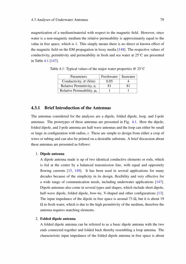
4.3 Analyses of Underwater Antennas 79
magnetization of a medium/material with respect to the magnetic field. However, sincewater is a non-magnetic medium the relative permeability is approximately equal to thevalue in free space, which is 1. This simply means there is no direct or known effect ofthe magnetic field on the EM propagation in lossy media [148]. The respective values ofconductivity, permittivity and permeability in fresh and sea water at 25C are presentedin Table 4.1 [147].
Table 4.1: Typical values of the major water properties @ 25C
Parameters Freshwater SeawaterConductivity, σ (S/m) 0.05 4
Relative Permittivity, εr 81 81Relative Permeability, µr 1 1
4.3.1 Brief Introduction of the Antennas
The antennas considered for the analyses are a dipole, folded dipole, loop, and J-poleantennas. The prototypes of these antennas are presented in Fig. 4.1. Here the dipole,folded dipole, and J-pole antenna are half wave antennas and the loop can either be smallor large in configuration with radius, r. These are simple to design from either a crop ofwires or tubing and can also be printed on a desirable substrate. A brief discussion aboutthese antennas are presented as follows:
1. Dipole antennaA dipole antenna made is up of two identical conductive elements or rods, whichis fed at the center by a balanced transmission line, with equal and oppositelyflowing currents [15, 149]. It has been used in several applications for manydecades because of the simplicity in its design, flexibility and very effective fora wide range of communication needs, including underwater applications [147].Dipole antennas also come in several types and shapes, which include short dipole,half-wave dipole, folded dipole, bow-tie, V-shaped and other configurations [13].The input impedance of the dipole in free space is around 73 Ω, but it is about 19Ω in fresh water, which is due to the high permittivity of the medium, therefore theantenna requires matching elements.
2. Folded dipole antennaA folded dipole antenna can be referred to as a basic dipole antenna with the twoends connected together and folded back thereby resembling a loop antenna. Thecharacteristic input impedance of the folded dipole antenna in free space is about
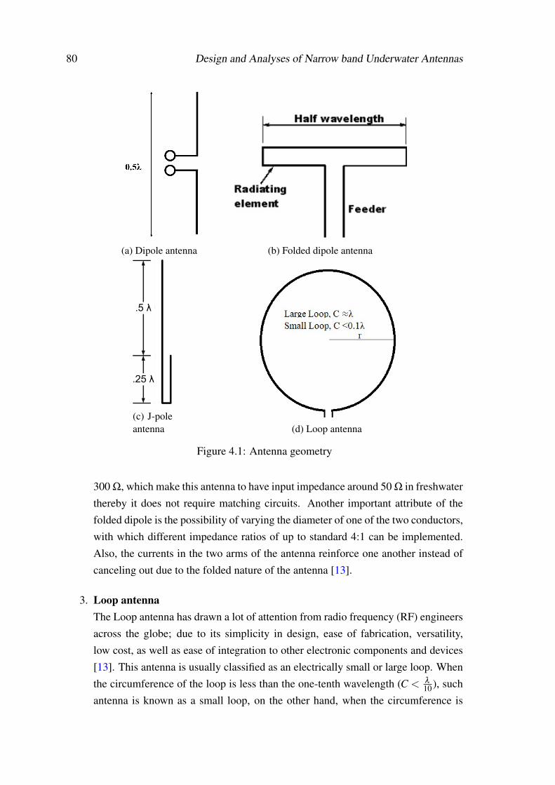
80 Design and Analyses of Narrow band Underwater Antennas
(a) Dipole antenna (b) Folded dipole antenna
(c) J-poleantenna (d) Loop antenna
Figure 4.1: Antenna geometry
300 Ω, which make this antenna to have input impedance around 50 Ω in freshwaterthereby it does not require matching circuits. Another important attribute of thefolded dipole is the possibility of varying the diameter of one of the two conductors,with which different impedance ratios of up to standard 4:1 can be implemented.Also, the currents in the two arms of the antenna reinforce one another instead ofcanceling out due to the folded nature of the antenna [13].
3. Loop antennaThe Loop antenna has drawn a lot of attention from radio frequency (RF) engineersacross the globe; due to its simplicity in design, ease of fabrication, versatility,low cost, as well as ease of integration to other electronic components and devices[13]. This antenna is usually classified as an electrically small or large loop. Whenthe circumference of the loop is less than the one-tenth wavelength (C < λ
10 ), suchantenna is known as a small loop, on the other hand, when the circumference is
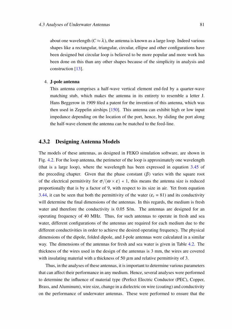
4.3 Analyses of Underwater Antennas 81
about one wavelength (C≈ λ ), the antenna is known as a large loop. Indeed variousshapes like a rectangular, triangular, circular, ellipse and other configurations havebeen designed but circular loop is believed to be more popular and more work hasbeen done on this than any other shapes because of the simplicity in analysis andconstruction [13].
4. J-pole antennaThis antenna comprises a half-wave vertical element end-fed by a quarter-wavematching stub, which makes the antenna in its entirety to resemble a letter J.Hans Beggerow in 1909 filed a patent for the invention of this antenna, which wasthen used in Zeppelin airships [150]. This antenna can exhibit high or low inputimpedance depending on the location of the port, hence, by sliding the port alongthe half-wave element the antenna can be matched to the feed-line.
4.3.2 Designing Antenna Models
The models of these antennas, as designed in FEKO simulation software, are shown inFig. 4.2. For the loop antenna, the perimeter of the loop is approximately one wavelength(that is a large loop), where the wavelength has been expressed in equation 3.45 ofthe preceding chapter. Given that the phase constant (β ) varies with the square rootof the electrical permitivity for σ/(ω × ε) « 1, this means the antenna size is reducedproportionally that is by a factor of 9, with respect to its size in air. Yet from equation3.44, it can be seen that both the permittivity of the water (εr = 81) and its conductivitywill determine the final dimensions of the antennas. In this regards, the medium is freshwater and therefore the conductivity is 0.05 S/m. The antennas are designed for anoperating frequency of 40 MHz. Thus, for such antennas to operate in fresh and seawater, different configurations of the antennas are required for each medium due to thedifferent conductivities in order to achieve the desired operating frequency. The physicaldimensions of the dipole, folded dipole, and J-pole antennas were calculated in a similarway. The dimensions of the antennas for fresh and sea water is given in Table 4.2. Thethickness of the wires used in the design of the antennas is 3 mm, the wires are coveredwith insulating material with a thickness of 50 µm and relative permittivity of 3.
Thus, in the analyses of these antennas, it is important to determine various parametersthat can affect their performance in any medium. Hence, several analyses were performedto determine the influence of material type (Perfect Electric Conductor (PEC), Copper,Brass, and Aluminum), wire size, change in a dielectric on wire (coating) and conductivityon the performance of underwater antennas. These were performed to ensure that the
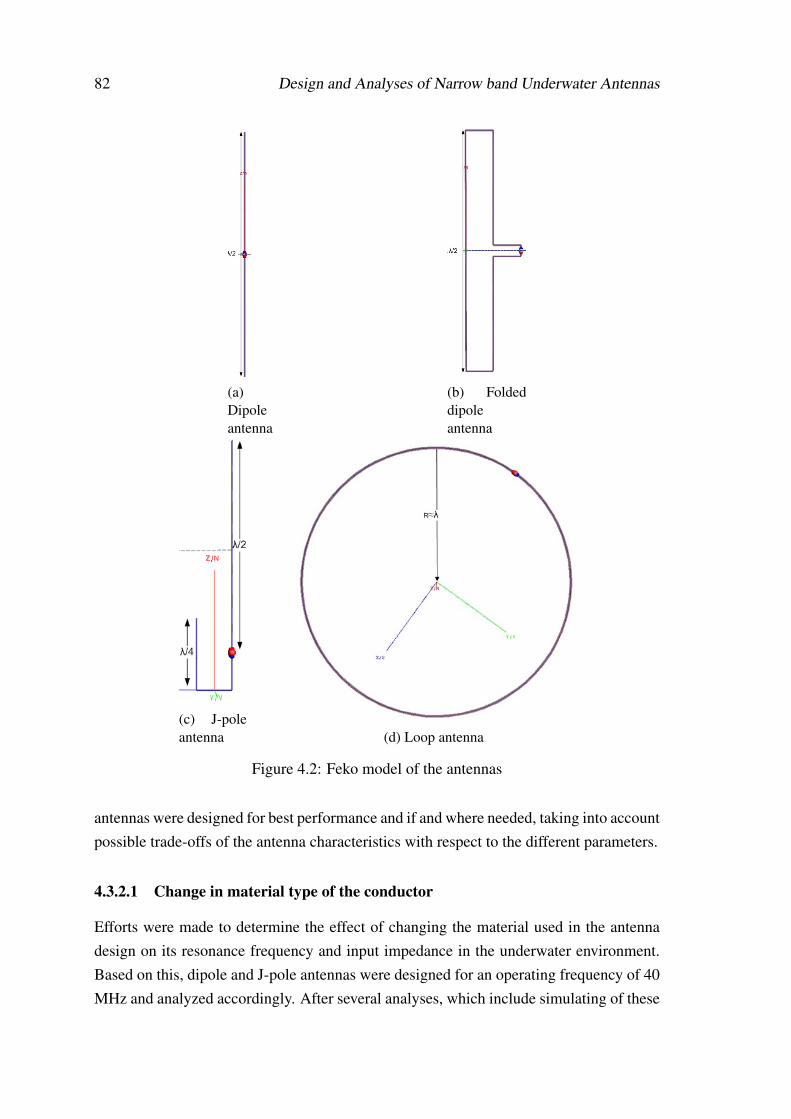
82 Design and Analyses of Narrow band Underwater Antennas
(a)Dipoleantenna
(b) Foldeddipoleantenna
(c) J-poleantenna (d) Loop antenna
Figure 4.2: Feko model of the antennas
antennas were designed for best performance and if and where needed, taking into accountpossible trade-offs of the antenna characteristics with respect to the different parameters.
4.3.2.1 Change in material type of the conductor
Efforts were made to determine the effect of changing the material used in the antennadesign on its resonance frequency and input impedance in the underwater environment.Based on this, dipole and J-pole antennas were designed for an operating frequency of 40MHz and analyzed accordingly. After several analyses, which include simulating of these
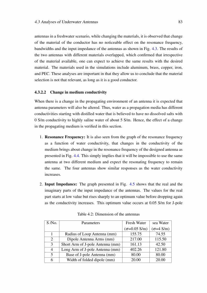
4.3 Analyses of Underwater Antennas 83
antennas in a freshwater scenario, while changing the materials, it is observed that changeof the material of the conductor has no noticeable effect on the resonance frequency,bandwidths and the input impedance of the antennas as shown in Fig. 4.3. The results ofthe two antennas with different materials overlapped, which confirmed that irrespectiveof the material available, one can expect to achieve the same results with the desiredmaterial. The materials used in the simulations include aluminum, brass, copper, iron,and PEC. These analyses are important in that they allow us to conclude that the materialselection is not that relevant, as long as it is a good conductor.
4.3.2.2 Change in medium conductivity
When there is a change in the propagating environment of an antenna it is expected thatantenna parameters will also be altered. Thus, water as a propagation media has differentconductivities starting with distilled water that is believed to have no dissolved salts with0 S/m conductivity to highly saline water of about 5 S/m. Hence, the effect of a changein the propagating medium is verified in this section.
1. Resonance Frequency: It is also seen from the graph of the resonance frequencyas a function of water conductivity, that changes in the conductivity of themedium brings about change in the resonance frequency of the designed antenna aspresented in Fig. 4.4. This simply implies that it will be impossible to use the sameantenna at two different medium and expect the resonating frequency to remainthe same. The four antennas show similar responses as the water conductivityincreases.
2. Input Impedance: The graph presented in Fig. 4.5 shows that the real and theimaginary parts of the input impedance of the antennas. The values for the realpart starts at low value but rises sharply to an optimum value before dropping againas the conductivity increases. This optimum value occurs at 0.05 S/m for J-pole
Table 4.2: Dimension of the antennas
S /No. Parameters Fresh Water sea Water(σ=0.05 S/m) (σ=4 S/m)
1 Radius of Loop Antenna (mm) 155.75 74.552 Dipole Antenna Arms (mm) 217.00 115.503 Short Arm of J-pole Antenna (mm) 161.13 42.504 Long Arm of J-pole Antenna (mm) 402.26 121.805 Base of J-pole Antenna (mm) 80.00 80.006 Width of folded dipole (mm) 20.00 20.00
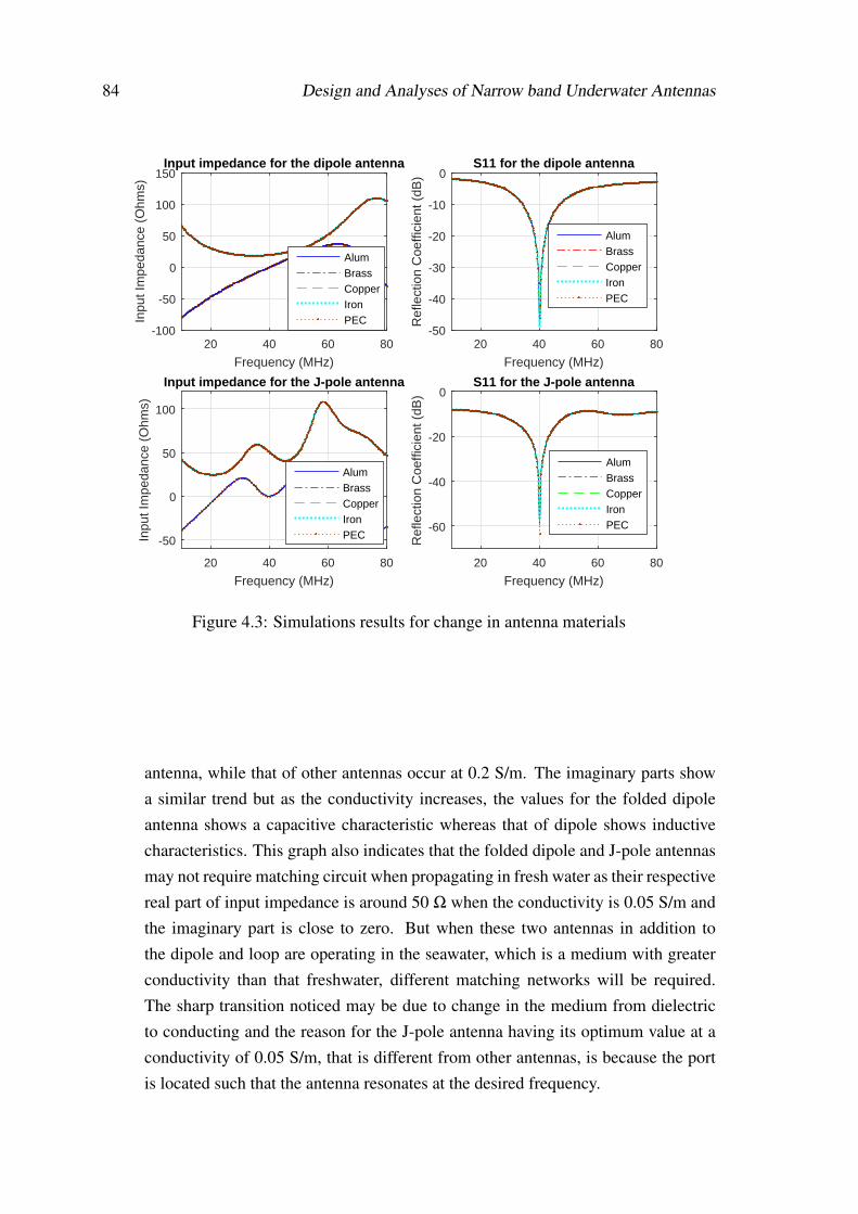
84 Design and Analyses of Narrow band Underwater Antennas
20 40 60 80
Frequency (MHz)
-100
-50
0
50
100
150
Inpu
t Im
peda
nce
(Ohm
s)
Input impedance for the dipole antenna
AlumBrassCopperIronPEC
20 40 60 80
Frequency (MHz)
-50
0
50
100
Inpu
t Im
peda
nce
(Ohm
s)
Input impedance for the J-pole antenna
AlumBrassCopperIronPEC
20 40 60 80
Frequency (MHz)
-50
-40
-30
-20
-10
0
Ref
lect
ion
Coe
ffici
ent (
dB)
S11 for the dipole antenna
AlumBrassCopperIronPEC
20 40 60 80
Frequency (MHz)
-60
-40
-20
0
Ref
lect
ion
Coe
ffici
ent (
dB)
S11 for the J-pole antenna
AlumBrassCopperIronPEC
Figure 4.3: Simulations results for change in antenna materials
antenna, while that of other antennas occur at 0.2 S/m. The imaginary parts showa similar trend but as the conductivity increases, the values for the folded dipoleantenna shows a capacitive characteristic whereas that of dipole shows inductivecharacteristics. This graph also indicates that the folded dipole and J-pole antennasmay not require matching circuit when propagating in fresh water as their respectivereal part of input impedance is around 50 Ω when the conductivity is 0.05 S/m andthe imaginary part is close to zero. But when these two antennas in addition tothe dipole and loop are operating in the seawater, which is a medium with greaterconductivity than that freshwater, different matching networks will be required.The sharp transition noticed may be due to change in the medium from dielectricto conducting and the reason for the J-pole antenna having its optimum value at aconductivity of 0.05 S/m, that is different from other antennas, is because the portis located such that the antenna resonates at the desired frequency.
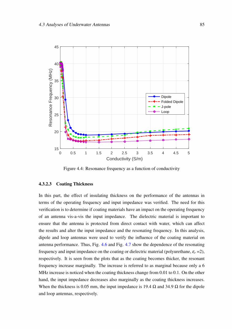
4.3 Analyses of Underwater Antennas 85
0 0.5 1 1.5 2 2.5 3 3.5 4 4.5 5
Conductivity (S/m)
15
20
25
30
35
40
45R
eson
ance
Fre
quen
cy (
MH
z)
DipoleFolded DipoleJ-poleLoop
Figure 4.4: Resonance frequency as a function of conductivity
4.3.2.3 Coating Thickness
In this part, the effect of insulating thickness on the performance of the antennas interms of the operating frequency and input impedance was verified. The need for thisverification is to determine if coating materials have an impact on the operating frequencyof an antenna vis-a-vis the input impedance. The dielectric material is important toensure that the antenna is protected from direct contact with water, which can affectthe results and alter the input impedance and the resonating frequency. In this analysis,dipole and loop antennas were used to verify the influence of the coating material onantenna performance. Thus, Fig. 4.6 and Fig. 4.7 show the dependence of the resonatingfrequency and input impedance on the coating or dielectric material (polyurethane, εr =2),respectively. It is seen from the plots that as the coating becomes thicker, the resonantfrequency increase marginally. The increase is referred to as marginal because only a 6MHz increase is noticed when the coating thickness change from 0.01 to 0.1. On the otherhand, the input impedance decreases also marginally as the coating thickness increases.When the thickness is 0.05 mm, the input impedance is 19.4 Ω and 34.9 Ω for the dipoleand loop antennas, respectively.
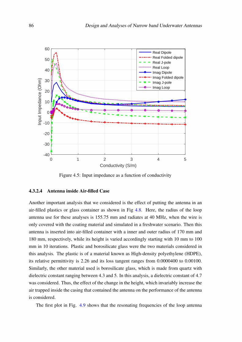
86 Design and Analyses of Narrow band Underwater Antennas
0 1 2 3 4 5
Conductivity (S/m)
-40
-30
-20
-10
0
10
20
30
40
50
60
Inpu
t Im
peda
nce
(Ohm
)
Real DipoleReal Folded dipoleReal J-poleReal LoopImag DipoleImag Folded dipoleImag J-poleImag Loop
Figure 4.5: Input impedance as a function of conductivity
4.3.2.4 Antenna inside Air-filled Case
Another important analysis that we considered is the effect of putting the antenna in anair-filled plastics or glass container as shown in Fig 4.8. Here, the radius of the loopantenna use for these analyses is 155.75 mm and radiates at 40 MHz, when the wire isonly covered with the coating material and simulated in a freshwater scenario. Then thisantenna is inserted into air-filled container with a inner and outer radius of 170 mm and180 mm, respectively, while its height is varied accordingly starting with 10 mm to 100mm in 10 iterations. Plastic and borosilicate glass were the two materials considered inthis analysis. The plastic is of a material known as High-density polyethylene (HDPE),its relative permittivity is 2.26 and its loss tangent ranges from 0.0000400 to 0.00100.Similarly, the other material used is borosilicate glass, which is made from quartz withdielectric constant ranging between 4.3 and 5. In this analysis, a dielectric constant of 4.7was considered. Thus, the effect of the change in the height, which invariably increase theair trapped inside the casing that contained the antenna on the performance of the antennais considered.
The first plot in Fig. 4.9 shows that the resonating frequencies of the loop antenna
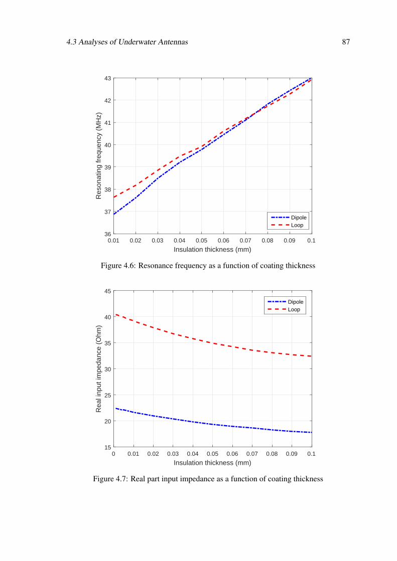
4.3 Analyses of Underwater Antennas 87
0.01 0.02 0.03 0.04 0.05 0.06 0.07 0.08 0.09 0.1
Insulation thickness (mm)
36
37
38
39
40
41
42
43
Res
onat
ing
freq
uenc
y (M
Hz)
DipoleLoop
Figure 4.6: Resonance frequency as a function of coating thickness
0 0.01 0.02 0.03 0.04 0.05 0.06 0.07 0.08 0.09 0.1
Insulation thickness (mm)
15
20
25
30
35
40
45
Rea
l inp
ut im
peda
nce
(Ohm
)
DipoleLoop
Figure 4.7: Real part input impedance as a function of coating thickness
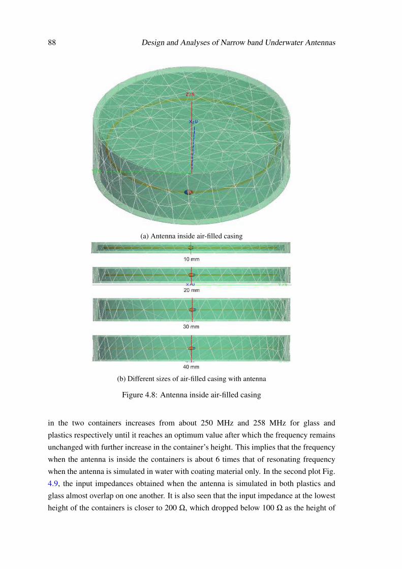
88 Design and Analyses of Narrow band Underwater Antennas
(a) Antenna inside air-filled casing
(b) Different sizes of air-filled casing with antenna
Figure 4.8: Antenna inside air-filled casing
in the two containers increases from about 250 MHz and 258 MHz for glass andplastics respectively until it reaches an optimum value after which the frequency remainsunchanged with further increase in the container’s height. This implies that the frequencywhen the antenna is inside the containers is about 6 times that of resonating frequencywhen the antenna is simulated in water with coating material only. In the second plot Fig.4.9, the input impedances obtained when the antenna is simulated in both plastics andglass almost overlap on one another. It is also seen that the input impedance at the lowestheight of the containers is closer to 200 Ω, which dropped below 100 Ω as the height of
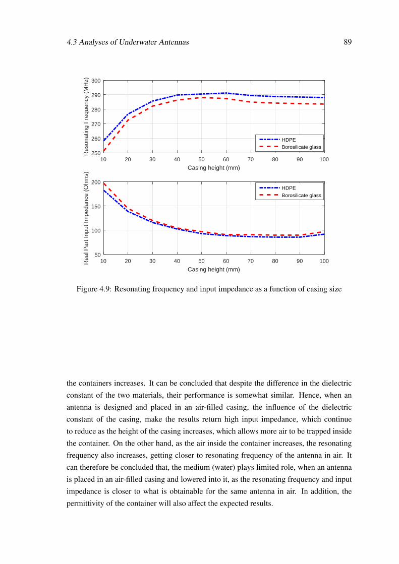
4.3 Analyses of Underwater Antennas 89
10 20 30 40 50 60 70 80 90 100
Casing height (mm)
250
260
270
280
290
300R
eson
atin
g F
requ
ency
(M
Hz)
HDPEBorosilicate glass
10 20 30 40 50 60 70 80 90 100
Casing height (mm)
50
100
150
200
Rea
l Par
t Inp
ut Im
peda
nce
(Ohm
s)
HDPE
Borosilicate glass
Figure 4.9: Resonating frequency and input impedance as a function of casing size
the containers increases. It can be concluded that despite the difference in the dielectricconstant of the two materials, their performance is somewhat similar. Hence, when anantenna is designed and placed in an air-filled casing, the influence of the dielectricconstant of the casing, make the results return high input impedance, which continueto reduce as the height of the casing increases, which allows more air to be trapped insidethe container. On the other hand, as the air inside the container increases, the resonatingfrequency also increases, getting closer to resonating frequency of the antenna in air. Itcan therefore be concluded that, the medium (water) plays limited role, when an antennais placed in an air-filled casing and lowered into it, as the resonating frequency and inputimpedance is closer to what is obtainable for the same antenna in air. In addition, thepermittivity of the container will also affect the expected results.
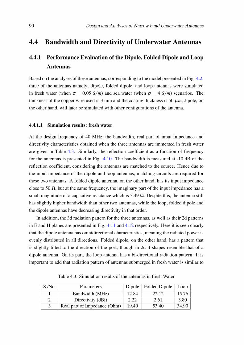
90 Design and Analyses of Narrow band Underwater Antennas
4.4 Bandwidth and Directivity of Underwater Antennas
4.4.1 Performance Evaluation of the Dipole, Folded Dipole and LoopAntennas
Based on the analyses of these antennas, corresponding to the model presented in Fig. 4.2,three of the antennas namely; dipole, folded dipole, and loop antennas were simulatedin fresh water (when σ = 0.05 S/m) and sea water (when σ = 4 S/m) scenarios. Thethickness of the copper wire used is 3 mm and the coating thickness is 50 µm, J-pole, onthe other hand, will later be simulated with other configurations of the antenna.
4.4.1.1 Simulation results: fresh water
At the design frequency of 40 MHz, the bandwidth, real part of input impedance anddirectivity characteristics obtained when the three antennas are immersed in fresh waterare given in Table 4.3. Similarly, the reflection coefficient as a function of frequencyfor the antennas is presented in Fig. 4.10. The bandwidth is measured at -10 dB of thereflection coefficient, considering the antennas are matched to the source. Hence due tothe input impedance of the dipole and loop antennas, matching circuits are required forthese two antennas. A folded dipole antenna, on the other hand, has its input impedanceclose to 50 Ω, but at the same frequency, the imaginary part of the input impedance has asmall magnitude of a capacitive reactance which is 3.49 Ω. Despite this, the antenna stillhas slightly higher bandwidth than other two antennas, while the loop, folded dipole andthe dipole antennas have decreasing directivity in that order.
In addition, the 3d radiation pattern for the three antennas, as well as their 2d patternsin E and H planes are presented in Fig. 4.11 and 4.12 respectively. Here it is seen clearlythat the dipole antenna has omnidirectional characteristics, meaning the radiated power isevenly distributed in all directions. Folded dipole, on the other hand, has a pattern thatis slightly tilted to the direction of the port, though in 2d it shapes resemble that of adipole antenna. On its part, the loop antenna has a bi-directional radiation pattern. It isimportant to add that radiation pattern of antennas submerged in fresh water is similar to
Table 4.3: Simulation results of the antennas in fresh Water
S /No. Parameters Dipole Folded Dipole Loop1 Bandwidth (MHz) 12.84 22.12 15.762 Directivity (dBi) 2.22 2.61 3.803 Real part of Impedance (Ohm) 19.40 53.40 34.90
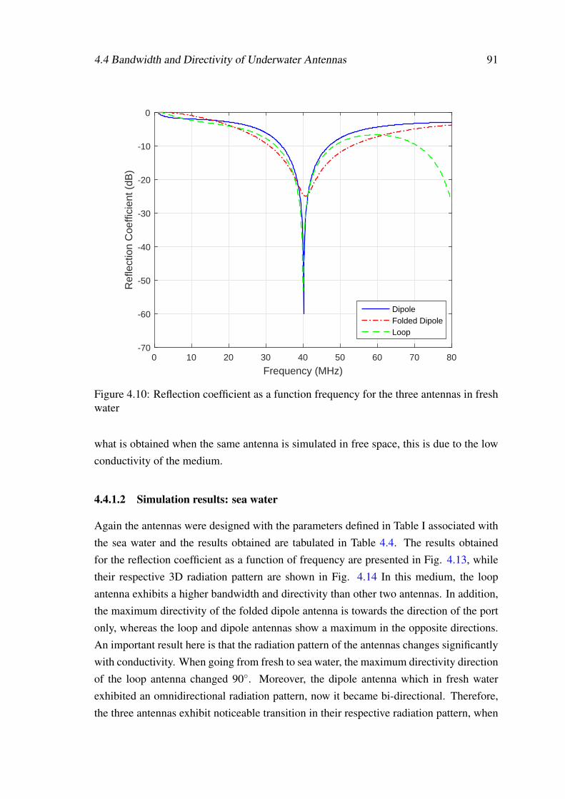
4.4 Bandwidth and Directivity of Underwater Antennas 91
0 10 20 30 40 50 60 70 80
Frequency (MHz)
-70
-60
-50
-40
-30
-20
-10
0
Ref
lect
ion
Coe
ffici
ent (
dB)
DipoleFolded DipoleLoop
Figure 4.10: Reflection coefficient as a function frequency for the three antennas in freshwater
what is obtained when the same antenna is simulated in free space, this is due to the lowconductivity of the medium.
4.4.1.2 Simulation results: sea water
Again the antennas were designed with the parameters defined in Table I associated withthe sea water and the results obtained are tabulated in Table 4.4. The results obtainedfor the reflection coefficient as a function of frequency are presented in Fig. 4.13, whiletheir respective 3D radiation pattern are shown in Fig. 4.14 In this medium, the loopantenna exhibits a higher bandwidth and directivity than other two antennas. In addition,the maximum directivity of the folded dipole antenna is towards the direction of the portonly, whereas the loop and dipole antennas show a maximum in the opposite directions.An important result here is that the radiation pattern of the antennas changes significantlywith conductivity. When going from fresh to sea water, the maximum directivity directionof the loop antenna changed 90. Moreover, the dipole antenna which in fresh waterexhibited an omnidirectional radiation pattern, now it became bi-directional. Therefore,the three antennas exhibit noticeable transition in their respective radiation pattern, when
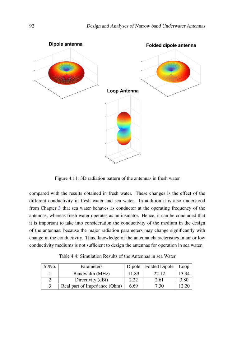
92 Design and Analyses of Narrow band Underwater Antennas
Dipole antenna Folded dipole antenna
Loop Antenna
Figure 4.11: 3D radiation pattern of the antennas in fresh water
compared with the results obtained in fresh water. These changes is the effect of thedifferent conductivity in fresh water and sea water. In addition it is also understoodfrom Chapter 3 that sea water behaves as conductor at the operating frequency of theantennas, whereas fresh water operates as an insulator. Hence, it can be concluded thatit is important to take into consideration the conductivity of the medium in the designof the antennas, because the major radiation parameters may change significantly withchange in the conductivity. Thus, knowledge of the antenna characteristics in air or lowconductivity mediums is not sufficient to design the antennas for operation in sea water.
Table 4.4: Simulation Results of the Antennas in sea Water
S /No. Parameters Dipole Folded Dipole Loop1 Bandwidth (MHz) 11.89 22.12 13.942 Directivity (dBi) 2.22 2.61 3.803 Real part of Impedance (Ohm) 6.69 7.30 12.20
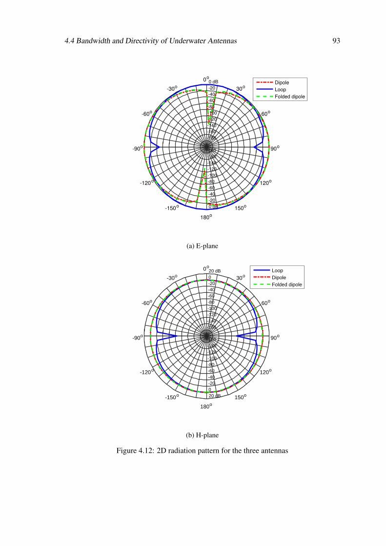
4.4 Bandwidth and Directivity of Underwater Antennas 93
-180
-180
-160
-160
-140
-140
-120
-120
-100
-100
-80
-80
-60
-60
-40
-40
-20
-20
0 dB
0 dB
90o
60o
30o
0o
-30o
-60o
-90o
-120o
-150o
180o
150o
120o
Dipole
Loop
Folded dipole
(a) E-plane
-160
-160
-140
-140
-120
-120
-100
-100
-80
-80
-60
-60
-40
-40
-20
-20
0
0
20 dB
20 dB
90o
60o
30o
0o
-30o
-60o
-90o
-120o
-150o
180o
150o
120o
LoopDipoleFolded dipole
(b) H-plane
Figure 4.12: 2D radiation pattern for the three antennas
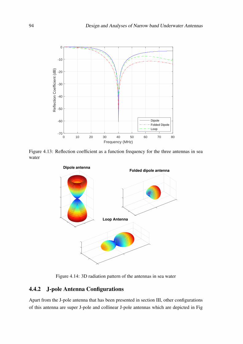
94 Design and Analyses of Narrow band Underwater Antennas
0 10 20 30 40 50 60 70 80
Frequency (MHz)
-70
-60
-50
-40
-30
-20
-10
0
Ref
lect
ion
Coe
ffici
ent (
dB)
DipoleFolded DipoleLoop
Figure 4.13: Reflection coefficient as a function frequency for the three antennas in seawater
Dipole antenna Folded dipole antenna
Loop Antenna
Figure 4.14: 3D radiation pattern of the antennas in sea water
4.4.2 J-pole Antenna Configurations
Apart from the J-pole antenna that has been presented in section III, other configurationsof this antenna are super J-pole and collinear J-pole antennas which are depicted in Fig
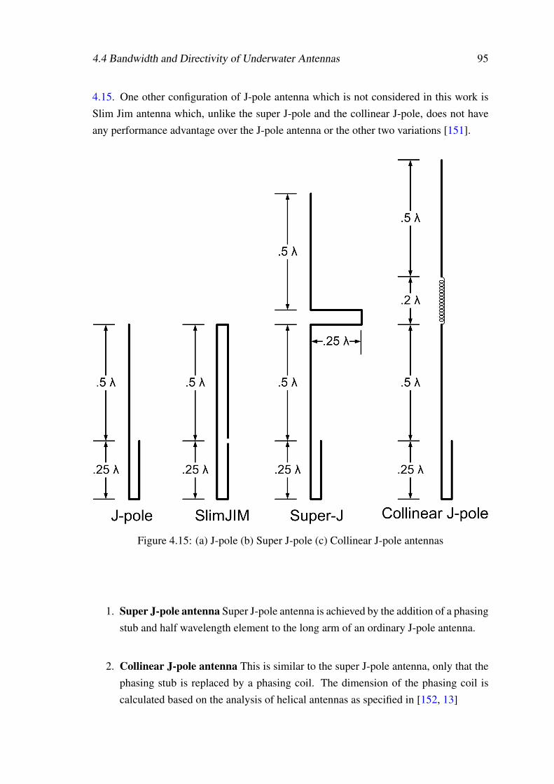
4.4 Bandwidth and Directivity of Underwater Antennas 95
4.15. One other configuration of J-pole antenna which is not considered in this work isSlim Jim antenna which, unlike the super J-pole and the collinear J-pole, does not haveany performance advantage over the J-pole antenna or the other two variations [151].
Figure 4.15: (a) J-pole (b) Super J-pole (c) Collinear J-pole antennas
1. Super J-pole antenna Super J-pole antenna is achieved by the addition of a phasingstub and half wavelength element to the long arm of an ordinary J-pole antenna.
2. Collinear J-pole antenna This is similar to the super J-pole antenna, only that thephasing stub is replaced by a phasing coil. The dimension of the phasing coil iscalculated based on the analysis of helical antennas as specified in [152, 13]
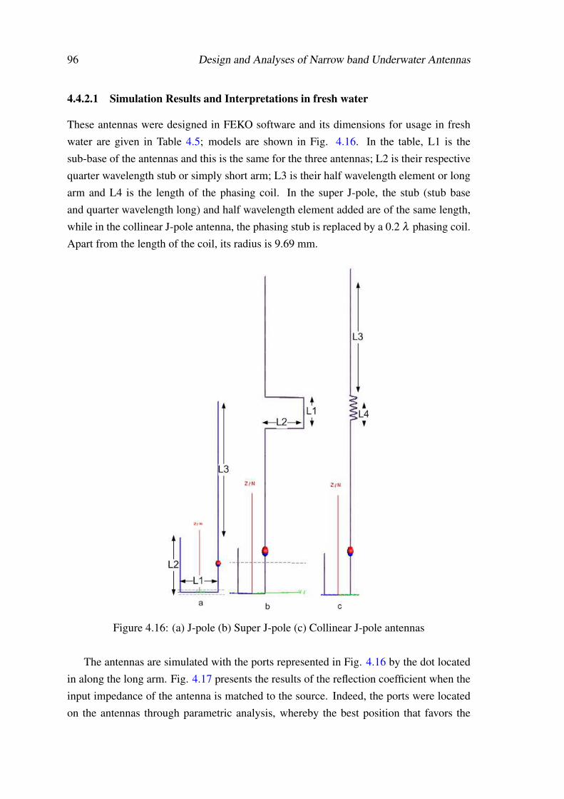
96 Design and Analyses of Narrow band Underwater Antennas
4.4.2.1 Simulation Results and Interpretations in fresh water
These antennas were designed in FEKO software and its dimensions for usage in freshwater are given in Table 4.5; models are shown in Fig. 4.16. In the table, L1 is thesub-base of the antennas and this is the same for the three antennas; L2 is their respectivequarter wavelength stub or simply short arm; L3 is their half wavelength element or longarm and L4 is the length of the phasing coil. In the super J-pole, the stub (stub baseand quarter wavelength long) and half wavelength element added are of the same length,while in the collinear J-pole antenna, the phasing stub is replaced by a 0.2 λ phasing coil.Apart from the length of the coil, its radius is 9.69 mm.
Figure 4.16: (a) J-pole (b) Super J-pole (c) Collinear J-pole antennas
The antennas are simulated with the ports represented in Fig. 4.16 by the dot locatedin along the long arm. Fig. 4.17 presents the results of the reflection coefficient when theinput impedance of the antenna is matched to the source. Indeed, the ports were locatedon the antennas through parametric analysis, whereby the best position that favors the
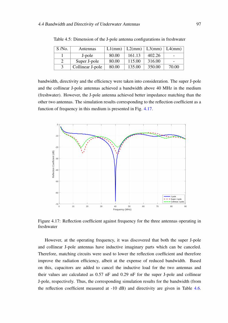
4.4 Bandwidth and Directivity of Underwater Antennas 97
Table 4.5: Dimension of the J-pole antenna configurations in freshwater
S /No. Antennas L1(mm) L2(mm) L3(mm) L4(mm)1 J-pole 80.00 161.13 402.26 -2 Super J-pole 80.00 115.00 316.00 -3 Collinear J-pole 80.00 135.00 350.00 70.00
bandwidth, directivity and the efficiency were taken into consideration. The super J-poleand the collinear J-pole antennas achieved a bandwidth above 40 MHz in the medium(freshwater). However, the J-pole antenna achieved better impedance matching than theother two antennas. The simulation results corresponding to the reflection coefficient as afunction of frequency in this medium is presented in Fig. 4.17.
0 10 20 30 40 50 60 70 80 90
Frequency (MHz)
-70
-60
-50
-40
-30
-20
-10
0
Ref
lect
ion
Coe
ffici
ent (
dB)
J-poleSuper J-poleCollinear J-pole
Figure 4.17: Reflection coefficient against frequency for the three antennas operating infreshwater
However, at the operating frequency, it was discovered that both the super J-poleand collinear J-pole antennas have inductive imaginary parts which can be canceled.Therefore, matching circuits were used to lower the reflection coefficient and thereforeimprove the radiation efficiency, albeit at the expense of reduced bandwidth. Basedon this, capacitors are added to cancel the inductive load for the two antennas andtheir values are calculated as 0.57 nF and 0.29 nF for the super J-pole and collinearJ-pole, respectively. Thus, the corresponding simulation results for the bandwidth (fromthe reflection coefficient measured at -10 dB) and directivity are given in Table 4.6.
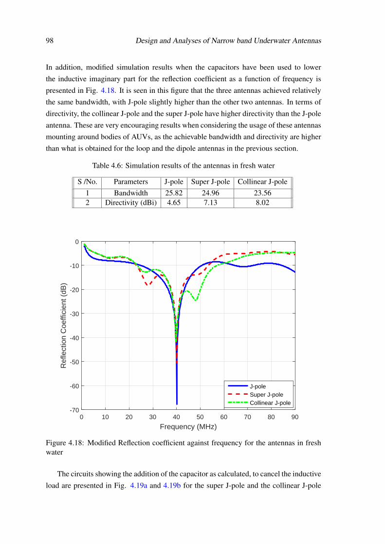
98 Design and Analyses of Narrow band Underwater Antennas
In addition, modified simulation results when the capacitors have been used to lowerthe inductive imaginary part for the reflection coefficient as a function of frequency ispresented in Fig. 4.18. It is seen in this figure that the three antennas achieved relativelythe same bandwidth, with J-pole slightly higher than the other two antennas. In terms ofdirectivity, the collinear J-pole and the super J-pole have higher directivity than the J-poleantenna. These are very encouraging results when considering the usage of these antennasmounting around bodies of AUVs, as the achievable bandwidth and directivity are higherthan what is obtained for the loop and the dipole antennas in the previous section.
Table 4.6: Simulation results of the antennas in fresh water
S /No. Parameters J-pole Super J-pole Collinear J-pole1 Bandwidth 25.82 24.96 23.562 Directivity (dBi) 4.65 7.13 8.02
0 10 20 30 40 50 60 70 80 90
Frequency (MHz)
-70
-60
-50
-40
-30
-20
-10
0
Ref
lect
ion
Coe
ffici
ent (
dB)
J-poleSuper J-poleCollinear J-pole
Figure 4.18: Modified Reflection coefficient against frequency for the antennas in freshwater
The circuits showing the addition of the capacitor as calculated, to cancel the inductiveload are presented in Fig. 4.19a and 4.19b for the super J-pole and the collinear J-pole
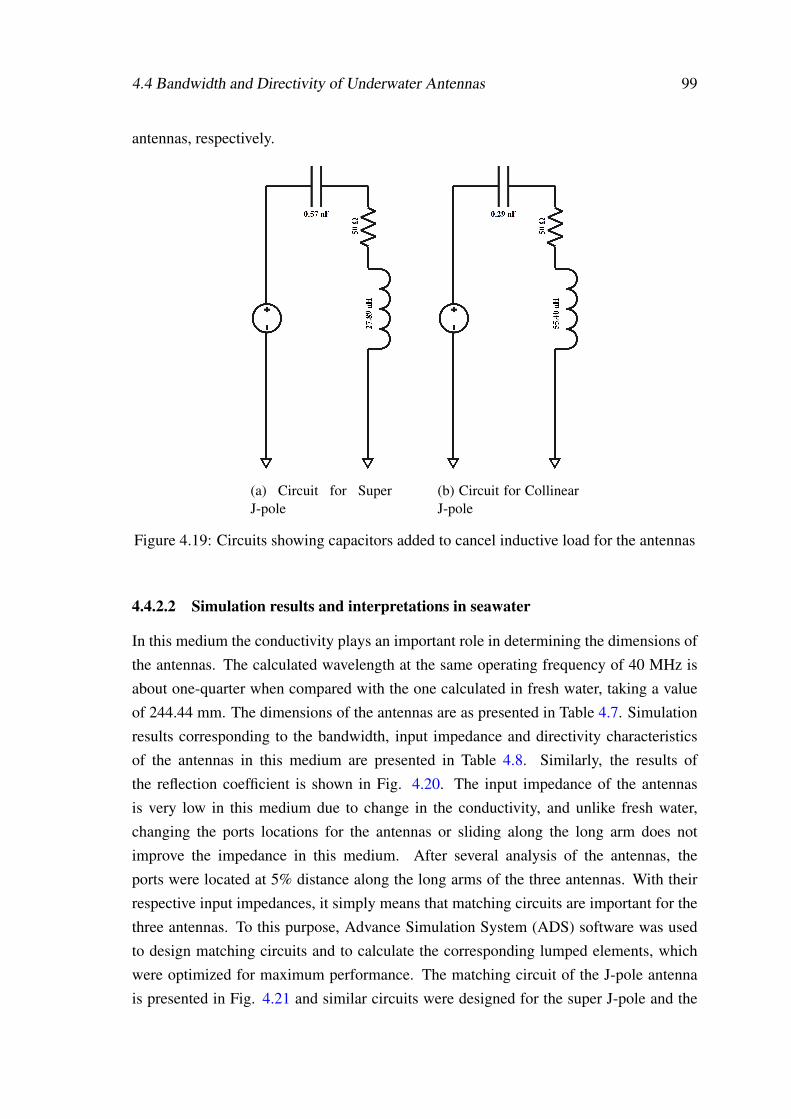
4.4 Bandwidth and Directivity of Underwater Antennas 99
antennas, respectively.
(a) Circuit for SuperJ-pole
(b) Circuit for CollinearJ-pole
Figure 4.19: Circuits showing capacitors added to cancel inductive load for the antennas
4.4.2.2 Simulation results and interpretations in seawater
In this medium the conductivity plays an important role in determining the dimensions ofthe antennas. The calculated wavelength at the same operating frequency of 40 MHz isabout one-quarter when compared with the one calculated in fresh water, taking a valueof 244.44 mm. The dimensions of the antennas are as presented in Table 4.7. Simulationresults corresponding to the bandwidth, input impedance and directivity characteristicsof the antennas in this medium are presented in Table 4.8. Similarly, the results ofthe reflection coefficient is shown in Fig. 4.20. The input impedance of the antennasis very low in this medium due to change in the conductivity, and unlike fresh water,changing the ports locations for the antennas or sliding along the long arm does notimprove the impedance in this medium. After several analysis of the antennas, theports were located at 5% distance along the long arms of the three antennas. With theirrespective input impedances, it simply means that matching circuits are important for thethree antennas. To this purpose, Advance Simulation System (ADS) software was usedto design matching circuits and to calculate the corresponding lumped elements, whichwere optimized for maximum performance. The matching circuit of the J-pole antennais presented in Fig. 4.21 and similar circuits were designed for the super J-pole and the
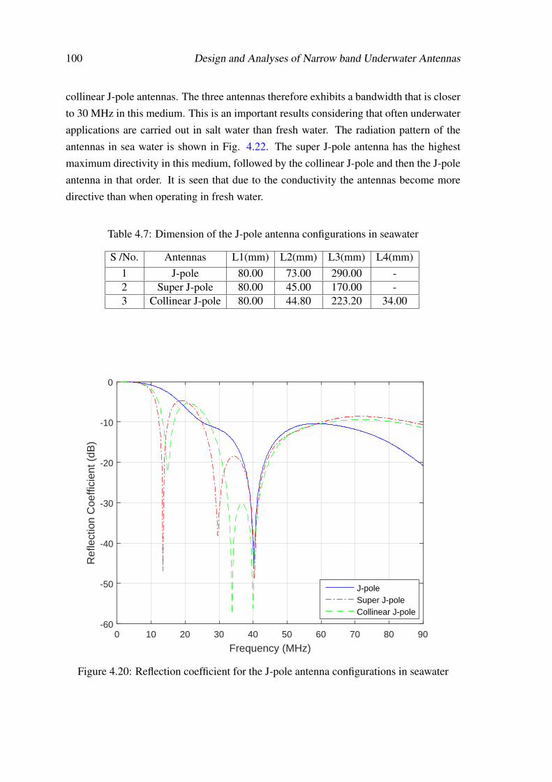
100 Design and Analyses of Narrow band Underwater Antennas
collinear J-pole antennas. The three antennas therefore exhibits a bandwidth that is closerto 30 MHz in this medium. This is an important results considering that often underwaterapplications are carried out in salt water than fresh water. The radiation pattern of theantennas in sea water is shown in Fig. 4.22. The super J-pole antenna has the highestmaximum directivity in this medium, followed by the collinear J-pole and then the J-poleantenna in that order. It is seen that due to the conductivity the antennas become moredirective than when operating in fresh water.
Table 4.7: Dimension of the J-pole antenna configurations in seawater
S /No. Antennas L1(mm) L2(mm) L3(mm) L4(mm)1 J-pole 80.00 73.00 290.00 -2 Super J-pole 80.00 45.00 170.00 -3 Collinear J-pole 80.00 44.80 223.20 34.00
0 10 20 30 40 50 60 70 80 90
Frequency (MHz)
-60
-50
-40
-30
-20
-10
0
Ref
lect
ion
Coe
ffici
ent (
dB)
J-poleSuper J-poleCollinear J-pole
Figure 4.20: Reflection coefficient for the J-pole antenna configurations in seawater
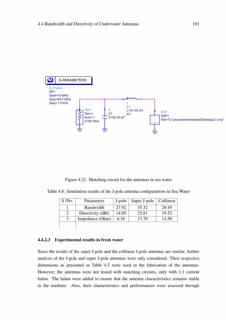
4.4 Bandwidth and Directivity of Underwater Antennas 101
Ref
1
S-PARAMETERS
Term
S_Param
C
L
S1PTerm1
SP1
C1
L1
SNP1
Z=50 OhmNum=1
Step=1.0 kHzStop=80.0 MHzStart=10 MHz
C=52.40 pFR=L=91.59 nH
File="C:\Users\Administrator\Desktop\L1.s1p"
Figure 4.21: Matching circuit for the antennas in sea water
Table 4.8: Simulation results of the J-pole antenna configurations in Sea Water
S /No. Parameters J-pole Super J-pole Collinear1 Bandwidth 27.92 35.32 28.452 Directivity (dBi) 14.05 25.81 19.523 Impedance (Ohm) 6.36 13.70 14.50
4.4.2.3 Experimental results in fresh water
Since the results of the super J-pole and the collinear J-pole antennas are similar, furtheranalysis of the J-pole and super J-pole antennas were only considered. Their respectivedimensions as presented in Table 4.5 were used in the fabrication of the antennas.However, the antennas were not tested with matching circuits, only with 1:1 currentbalun. The balun were added to ensure that the antenna characteristics remains stablein the medium. Also, their characteristics and performances were assessed through
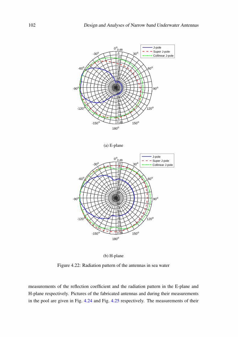
102 Design and Analyses of Narrow band Underwater Antennas
-45
-45
-40
-40
-35
-35
-30
-30
-25
-25
-20
-20
-15
-15
-10
-10
-5
-5
0 dB
0 dB
90o
60o
30o
0o
-30o
-60o
-90o
-120o
-150o
180o
150o
120o
J-poleSuper J-poleCollinear J-pole
(a) E-plane
-90
-90
-80
-80
-70
-70
-60
-60
-50
-50
-40
-40
-30
-30
-20
-20
-10
-10
0 dB
0 dB
90o
60o
30o
0o
-30o
-60o
-90o
-120o
-150o
180o
150o
120o
J-poleSuper J-poleCollinear J-pole
(b) H-plane
Figure 4.22: Radiation pattern of the antennas in sea water
measurements of the reflection coefficient and the radiation pattern in the E-plane andH-plane respectively. Pictures of the fabricated antennas and during their measurementsin the pool are given in Fig. 4.24 and Fig. 4.25 respectively. The measurements of their
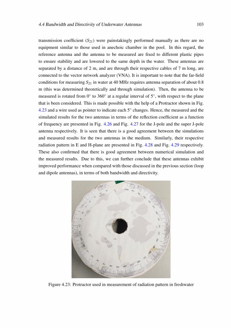
4.4 Bandwidth and Directivity of Underwater Antennas 103
transmission coefficient (S21) were painstakingly performed manually as there are noequipment similar to those used in anechoic chamber in the pool. In this regard, thereference antenna and the antenna to be measured are fixed to different plastic pipesto ensure stability and are lowered to the same depth in the water. These antennas areseparated by a distance of 2 m, and are through their respective cables of 7 m long, areconnected to the vector network analyzer (VNA). It is important to note that the far-fieldconditions for measuring S21 in water at 40 MHz requires antenna separation of about 0.8m (this was determined theoretically and through simulation). Then, the antenna to bemeasured is rotated from 0 to 360 at a regular interval of 5, with respect to the planethat is been considered. This is made possible with the help of a Protractor shown in Fig.4.23 and a wire used as pointer to indicate each 5 changes. Hence, the measured and thesimulated results for the two antennas in terms of the reflection coefficient as a functionof frequency are presented in Fig. 4.26 and Fig. 4.27 for the J-pole and the super J-poleantenna respectively. It is seen that there is a good agreement between the simulationsand measured results for the two antennas in the medium. Similarly, their respectiveradiation pattern in E and H-plane are presented in Fig. 4.28 and Fig. 4.29 respectively.These also confirmed that there is good agreement between numerical simulation andthe measured results. Due to this, we can further conclude that these antennas exhibitimproved performance when compared with those discussed in the previous section (loopand dipole antennas), in terms of both bandwidth and directivity.
Figure 4.23: Protractor used in measurement of radiation pattern in freshwater
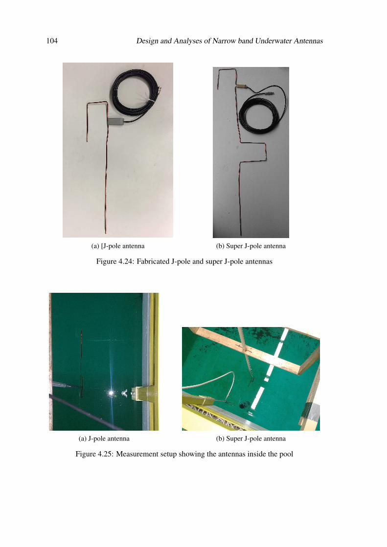
104 Design and Analyses of Narrow band Underwater Antennas
(a) [J-pole antenna (b) Super J-pole antenna
Figure 4.24: Fabricated J-pole and super J-pole antennas
(a) J-pole antenna (b) Super J-pole antenna
Figure 4.25: Measurement setup showing the antennas inside the pool
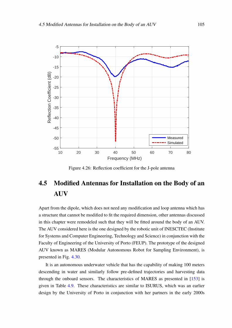
4.5 Modified Antennas for Installation on the Body of an AUV 105
10 20 30 40 50 60 70 80
Frequency (MHz)
-55
-50
-45
-40
-35
-30
-25
-20
-15
-10
-5R
efle
ctio
n C
oeffi
cien
t (dB
)
MeasuredSimulated
Figure 4.26: Reflection coefficient for the J-pole antenna
4.5 Modified Antennas for Installation on the Body of anAUV
Apart from the dipole, which does not need any modification and loop antenna which hasa structure that cannot be modified to fit the required dimension, other antennas discussedin this chapter were remodeled such that they will be fitted around the body of an AUV.The AUV considered here is the one designed by the robotic unit of INESCTEC (Institutefor Systems and Computer Engineering, Technology and Science) in conjunction with theFaculty of Engineering of the University of Porto (FEUP). The prototype of the designedAUV known as MARES (Modular Autonomous Robot for Sampling Environment), ispresented in Fig. 4.30.
It is an autonomous underwater vehicle that has the capability of making 100 metersdescending in water and similarly follow pre-defined trajectories and harvesting datathrough the onboard sensors. The characteristics of MARES as presented in [153] isgiven in Table 4.9. These characteristics are similar to ISURUS, which was an earlierdesign by the University of Porto in conjunction with her partners in the early 2000s
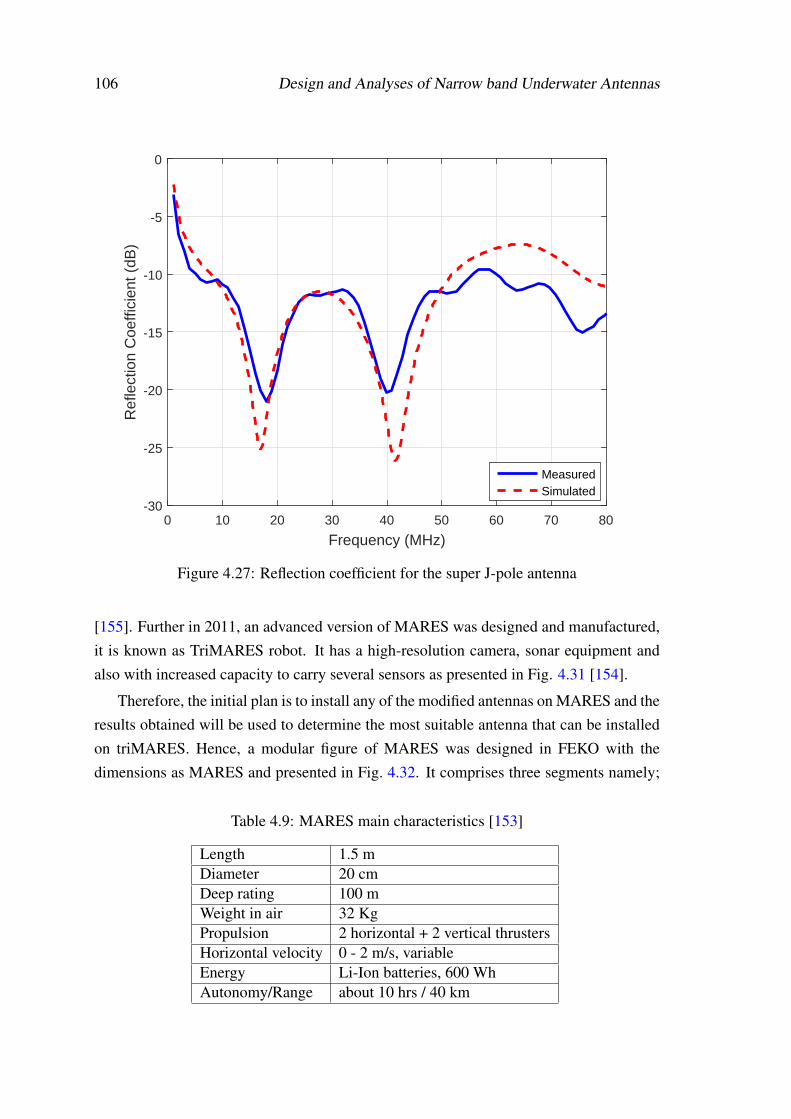
106 Design and Analyses of Narrow band Underwater Antennas
0 10 20 30 40 50 60 70 80
Frequency (MHz)
-30
-25
-20
-15
-10
-5
0
Ref
lect
ion
Coe
ffici
ent (
dB)
MeasuredSimulated
Figure 4.27: Reflection coefficient for the super J-pole antenna
[155]. Further in 2011, an advanced version of MARES was designed and manufactured,it is known as TriMARES robot. It has a high-resolution camera, sonar equipment andalso with increased capacity to carry several sensors as presented in Fig. 4.31 [154].
Therefore, the initial plan is to install any of the modified antennas on MARES and theresults obtained will be used to determine the most suitable antenna that can be installedon triMARES. Hence, a modular figure of MARES was designed in FEKO with thedimensions as MARES and presented in Fig. 4.32. It comprises three segments namely;
Table 4.9: MARES main characteristics [153]
Length 1.5 mDiameter 20 cmDeep rating 100 mWeight in air 32 KgPropulsion 2 horizontal + 2 vertical thrustersHorizontal velocity 0 - 2 m/s, variableEnergy Li-Ion batteries, 600 WhAutonomy/Range about 10 hrs / 40 km
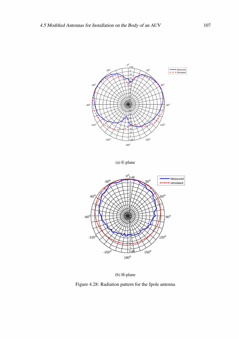
4.5 Modified Antennas for Installation on the Body of an AUV 107
-45
-45
-40
-40
-35
-35
-30
-30
-25
-25
-20
-20
-15
-15
-10
-10
-5
-5
0 dB
0 dB
90o
60o
30o
0o
-30o
-60o
-90o
-120o
-150o
180o
150o
120o
MeasuredSimulated
(a) E-plane
-9
-9
-8
-8
-7
-7
-6
-6
-5
-5
-4
-4
-3
-3
-2
-2
-1
-1
0 dB
0 dB
90o
60o
30o
0o
-30o
-60o
-90o
-120o
-150o
180o
150o
120o
Measuredsimulated
(b) H-plane
Figure 4.28: Radiation pattern for the Jpole antenna
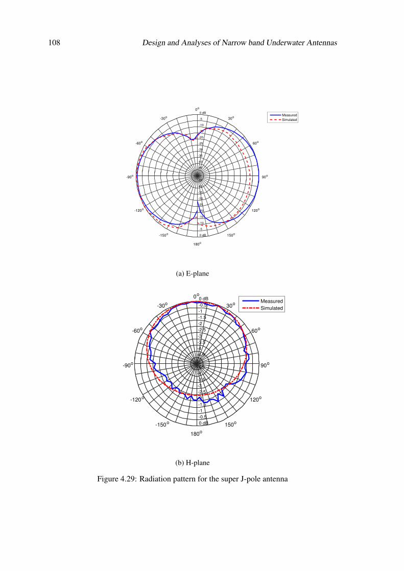
108 Design and Analyses of Narrow band Underwater Antennas
-45
-45
-40
-40
-35
-35
-30
-30
-25
-25
-20
-20
-15
-15
-10
-10
-5
-5
0 dB
0 dB
90o
60o
30o
0o
-30o
-60o
-90o
-120o
-150o
180o
150o
120o
Measured
Simulated
(a) E-plane
-4.5
-4.5
-4
-4
-3.5
-3.5
-3
-3
-2.5
-2.5
-2
-2
-1.5
-1.5
-1
-1
-0.5
-0.5
0 dB
0 dB
90o
60o
30o
0o
-30o
-60o
-90o
-120o
-150o
180o
150o
120o
Measured
Simulated
(b) H-plane
Figure 4.29: Radiation pattern for the super J-pole antenna
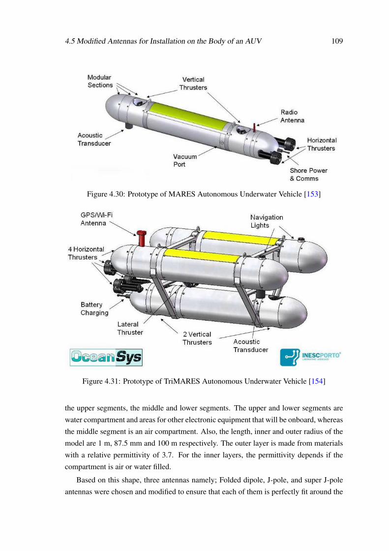
4.5 Modified Antennas for Installation on the Body of an AUV 109
Figure 4.30: Prototype of MARES Autonomous Underwater Vehicle [153]
Figure 4.31: Prototype of TriMARES Autonomous Underwater Vehicle [154]
the upper segments, the middle and lower segments. The upper and lower segments arewater compartment and areas for other electronic equipment that will be onboard, whereasthe middle segment is an air compartment. Also, the length, inner and outer radius of themodel are 1 m, 87.5 mm and 100 m respectively. The outer layer is made from materialswith a relative permittivity of 3.7. For the inner layers, the permittivity depends if thecompartment is air or water filled.
Based on this shape, three antennas namely; Folded dipole, J-pole, and super J-poleantennas were chosen and modified to ensure that each of them is perfectly fit around the
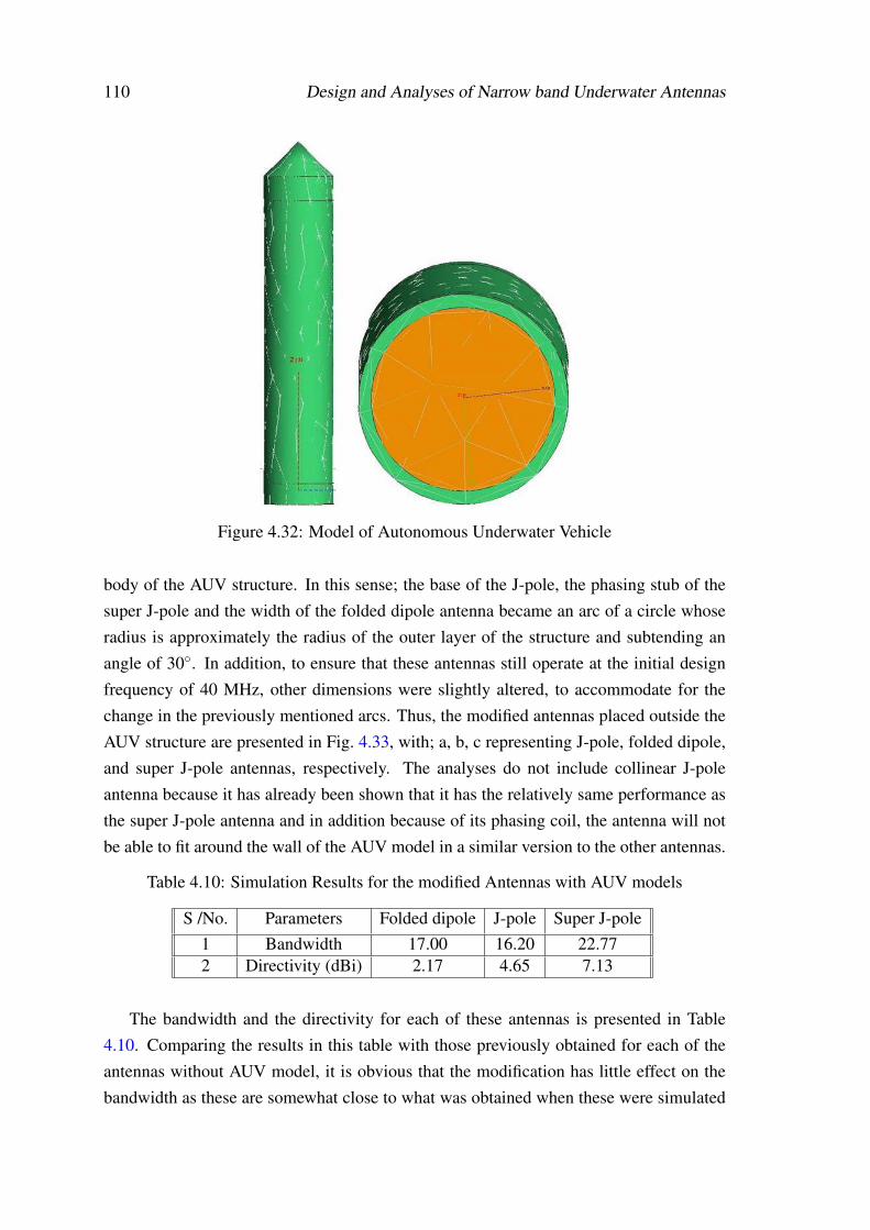
110 Design and Analyses of Narrow band Underwater Antennas
Figure 4.32: Model of Autonomous Underwater Vehicle
body of the AUV structure. In this sense; the base of the J-pole, the phasing stub of thesuper J-pole and the width of the folded dipole antenna became an arc of a circle whoseradius is approximately the radius of the outer layer of the structure and subtending anangle of 30. In addition, to ensure that these antennas still operate at the initial designfrequency of 40 MHz, other dimensions were slightly altered, to accommodate for thechange in the previously mentioned arcs. Thus, the modified antennas placed outside theAUV structure are presented in Fig. 4.33, with; a, b, c representing J-pole, folded dipole,and super J-pole antennas, respectively. The analyses do not include collinear J-poleantenna because it has already been shown that it has the relatively same performance asthe super J-pole antenna and in addition because of its phasing coil, the antenna will notbe able to fit around the wall of the AUV model in a similar version to the other antennas.
Table 4.10: Simulation Results for the modified Antennas with AUV models
S /No. Parameters Folded dipole J-pole Super J-pole1 Bandwidth 17.00 16.20 22.772 Directivity (dBi) 2.17 4.65 7.13
The bandwidth and the directivity for each of these antennas is presented in Table4.10. Comparing the results in this table with those previously obtained for each of theantennas without AUV model, it is obvious that the modification has little effect on thebandwidth as these are somewhat close to what was obtained when these were simulated
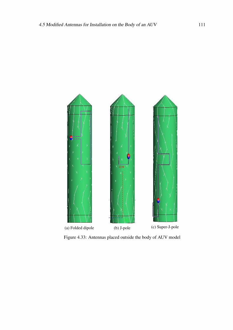
4.5 Modified Antennas for Installation on the Body of an AUV 111
(a) Folded dipole (b) J-pole (c) Super-J-pole
Figure 4.33: Antennas placed outside the body of AUV model
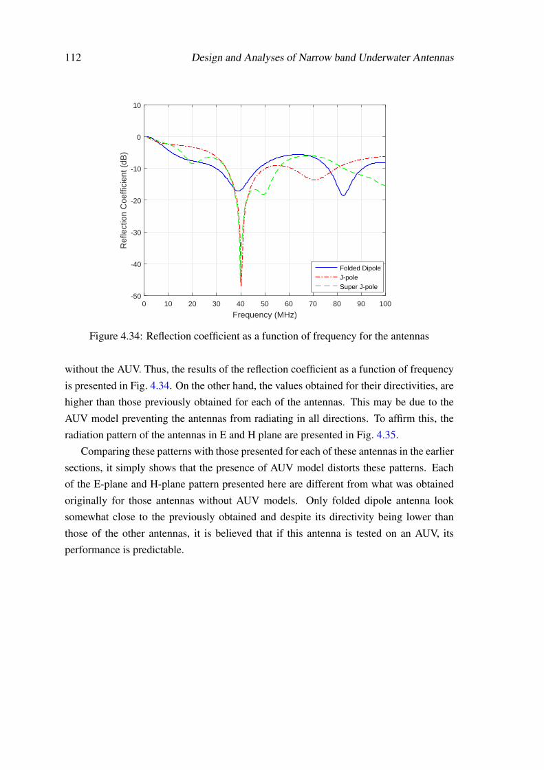
112 Design and Analyses of Narrow band Underwater Antennas
0 10 20 30 40 50 60 70 80 90 100
Frequency (MHz)
-50
-40
-30
-20
-10
0
10
Ref
lect
ion
Coe
ffici
ent (
dB)
Folded DipoleJ-poleSuper J-pole
Figure 4.34: Reflection coefficient as a function of frequency for the antennas
without the AUV. Thus, the results of the reflection coefficient as a function of frequencyis presented in Fig. 4.34. On the other hand, the values obtained for their directivities, arehigher than those previously obtained for each of the antennas. This may be due to theAUV model preventing the antennas from radiating in all directions. To affirm this, theradiation pattern of the antennas in E and H plane are presented in Fig. 4.35.
Comparing these patterns with those presented for each of these antennas in the earliersections, it simply shows that the presence of AUV model distorts these patterns. Eachof the E-plane and H-plane pattern presented here are different from what was obtainedoriginally for those antennas without AUV models. Only folded dipole antenna looksomewhat close to the previously obtained and despite its directivity being lower thanthose of the other antennas, it is believed that if this antenna is tested on an AUV, itsperformance is predictable.
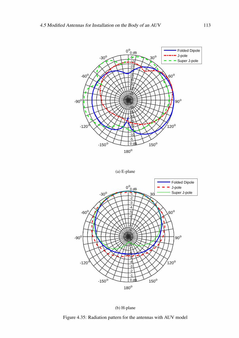
4.5 Modified Antennas for Installation on the Body of an AUV 113
-45
-45
-40
-40
-35
-35
-30
-30
-25
-25
-20
-20
-15
-15
-10
-10
-5
-5
0 dB
0 dB
90o
60o
30o
0o
-30o
-60o
-90o
-120o
-150o
180o
150o
120o
Folded DipoleJ-poleSuper J-pole
(a) E-plane
-9
-9
-8
-8
-7
-7
-6
-6
-5
-5
-4
-4
-3
-3
-2
-2
-1
-1
0 dB
0 dB
90o
60o
30o
0o
-30o
-60o
-90o
-120o
-150o
180o
150o
120o
Folded DipoleJ-poleSuper J-pole
(b) H-plane
Figure 4.35: Radiation pattern for the antennas with AUV model
114 Design and Analyses of Narrow band Underwater Antennas
4.6 Conclusion
In this chapter, analyses of various parameters that can affect the design and developmentof underwater antennas were given. In addition, the performance of narrowband antennaswith respect to the bandwidth and directivity has thus been presented. It is seen thatsuper J-pole and collinear J-pole antennas have higher bandwidth and directivity whencompared with other antennas presented in this chapter. Experimental results havebeen obtained of the reflection coefficient and radiation patterns, that match closely thenumerical simulation.
The conclusion drawn is that due to the physical structure of some of the antennaspresented in this chapter, it will be easier to fix such antenna around the body of an AUVmodel for onward data harvesting or communication with other underwater bodies. Butfixing two antennas of the same type may enhance performance due to the noticeableeffect of the AUV model on the radiation pattern of the antennas.
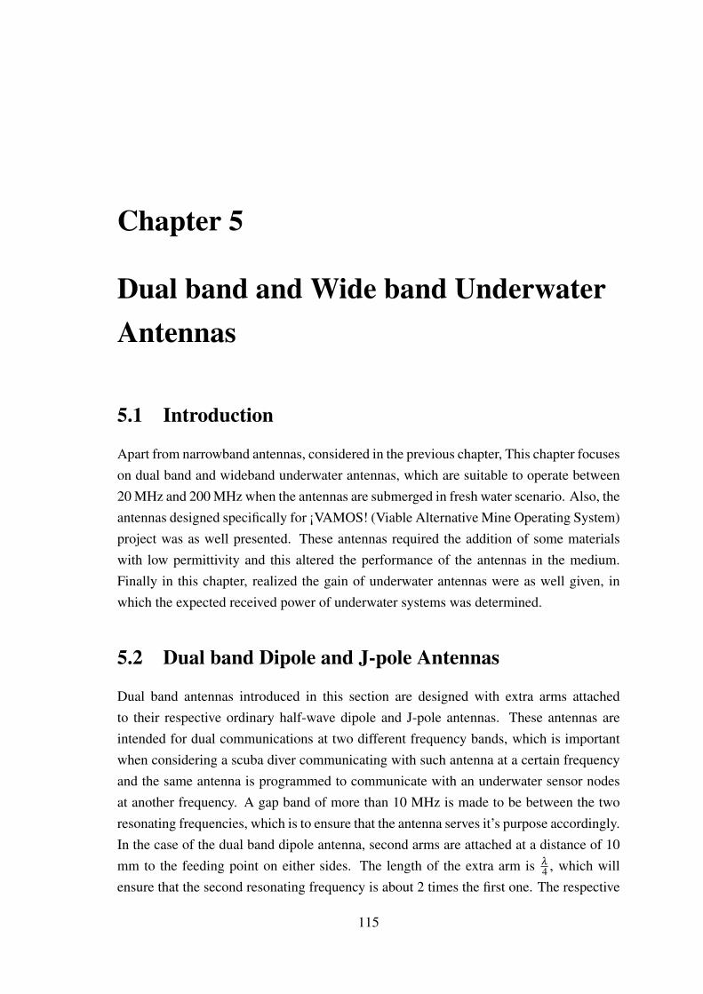
Chapter 5
Dual band and Wide band UnderwaterAntennas
5.1 Introduction
Apart from narrowband antennas, considered in the previous chapter, This chapter focuseson dual band and wideband underwater antennas, which are suitable to operate between20 MHz and 200 MHz when the antennas are submerged in fresh water scenario. Also, theantennas designed specifically for ¡VAMOS! (Viable Alternative Mine Operating System)project was as well presented. These antennas required the addition of some materialswith low permittivity and this altered the performance of the antennas in the medium.Finally in this chapter, realized the gain of underwater antennas were as well given, inwhich the expected received power of underwater systems was determined.
5.2 Dual band Dipole and J-pole Antennas
Dual band antennas introduced in this section are designed with extra arms attachedto their respective ordinary half-wave dipole and J-pole antennas. These antennas areintended for dual communications at two different frequency bands, which is importantwhen considering a scuba diver communicating with such antenna at a certain frequencyand the same antenna is programmed to communicate with an underwater sensor nodesat another frequency. A gap band of more than 10 MHz is made to be between the tworesonating frequencies, which is to ensure that the antenna serves it’s purpose accordingly.In the case of the dual band dipole antenna, second arms are attached at a distance of 10mm to the feeding point on either sides. The length of the extra arm is λ
4 , which willensure that the second resonating frequency is about 2 times the first one. The respective
115
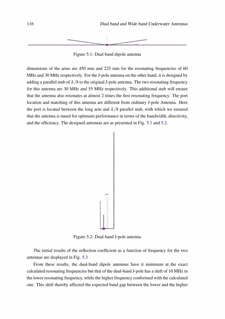
116 Dual band and Wide band Underwater Antennas
Figure 5.1: Dual band dipole antenna
dimensions of the arms are 450 mm and 225 mm for the resonating frequencies of 60MHz and 30 MHz respectively. For the J-pole antenna on the other hand, it is designed byadding a parallel stub of λ/8 to the original J-pole antenna. The two resonating frequencyfor this antenna are 30 MHz and 55 MHz respectively. This additional stub will ensurethat the antenna also resonates at almost 2 times the first resonating frequency. The portlocation and matching of this antenna are different from ordinary J-pole Antenna. Herethe port is located between the long arm and λ/8 parallel stub, with which we ensuredthat the antenna is tuned for optimum performance in terms of the bandwidth, directivity,and the efficiency. The designed antennas are as presented in Fig. 5.1 and 5.2.
Figure 5.2: Dual band J-pole antenna
The initial results of the reflection coefficient as a function of frequency for the twoantennas are displayed in Fig. 5.3
From these results, the dual-band dipole antennas have it minimum at the exactcalculated resonating frequencies but that of the dual-band J-pole has a shift of 10 MHz inthe lower resonating frequency, while the higher frequency conformed with the calculatedone. This shift thereby affected the expected band gap between the lower and the higher
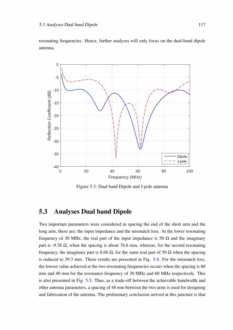
5.3 Analyses Dual band Dipole 117
resonating frequencies. Hence, further analyses will only focus on the dual-band dipoleantenna.
0 20 40 60 80 100
Frequency (MHz)
-40
-35
-30
-25
-20
-15
-10
-5
0
Ref
lect
ion
Coe
ffici
ent (
dB)
DipoleJ-pole
Figure 5.3: Dual band Dipole and J-pole antenna
5.3 Analyses Dual band Dipole
Two important parameters were considered in spacing the end of the short arm and thelong arm, these are; the input impedance and the mismatch loss. At the lower resonatingfrequency of 30 MHz, the real part of the input impedance is 50 Ω and the imaginarypart is -9.38 Ω, when the spacing is about 76.6 mm, whereas, for the second resonatingfrequency, the imaginary part is 8.68 Ω, for the same real part of 50 Ω when the spacingis reduced to 39.3 mm. These results are presented in Fig. 5.4. For the mismatch loss,the lowest value achieved at the two resonating frequencies occurs when the spacing is 60mm and 40 mm for the resonance frequency of 30 MHz and 60 MHz respectively. Thisis also presented in Fig. 5.5. Thus, as a trade-off between the achievable bandwidth andother antenna parameters, a spacing of 48 mm between the two arms is used for designingand fabrication of the antenna. The preliminary conclusion arrived at this juncture is that
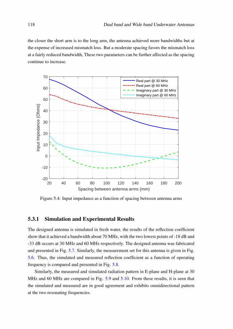
118 Dual band and Wide band Underwater Antennas
the closer the short arm is to the long arm, the antenna achieved more bandwidths but atthe expense of increased mismatch loss. But a moderate spacing favors the mismatch lossat a fairly reduced bandwidth, These two parameters can be further affected as the spacingcontinue to increase.
20 40 60 80 100 120 140 160 180 200
Spacing between antenna arms (mm)
-20
-10
0
10
20
30
40
50
60
70
Inpu
t Im
peda
nce
(Ohm
s)
Real part @ 30 MHzReal part @ 60 MHzImaginary part @ 30 MHzImaginary part @ 60 MHz
Figure 5.4: Input impedance as a function of spacing between antenna arms
5.3.1 Simulation and Experimental Results
The designed antenna is simulated in fresh water, the results of the reflection coefficientshow that it achieved a bandwidth about 70 MHz, with the two lowest points of -18 dB and-33 dB occurs at 30 MHz and 60 MHz respectively. The designed antenna was fabricatedand presented in Fig. 5.7. Similarly, the measurement set for this antenna is given in Fig.5.6. Thus, the simulated and measured reflection coefficient as a function of operatingfrequency is compared and presented in Fig. 5.8.
Similarly, the measured and simulated radiation pattern in E-plane and H-plane at 30MHz and 60 MHz are compared in Fig. 5.9 and 5.10. From these results, it is seen thatthe simulated and measured are in good agreement and exhibits omnidirectional patternat the two resonating frequencies.
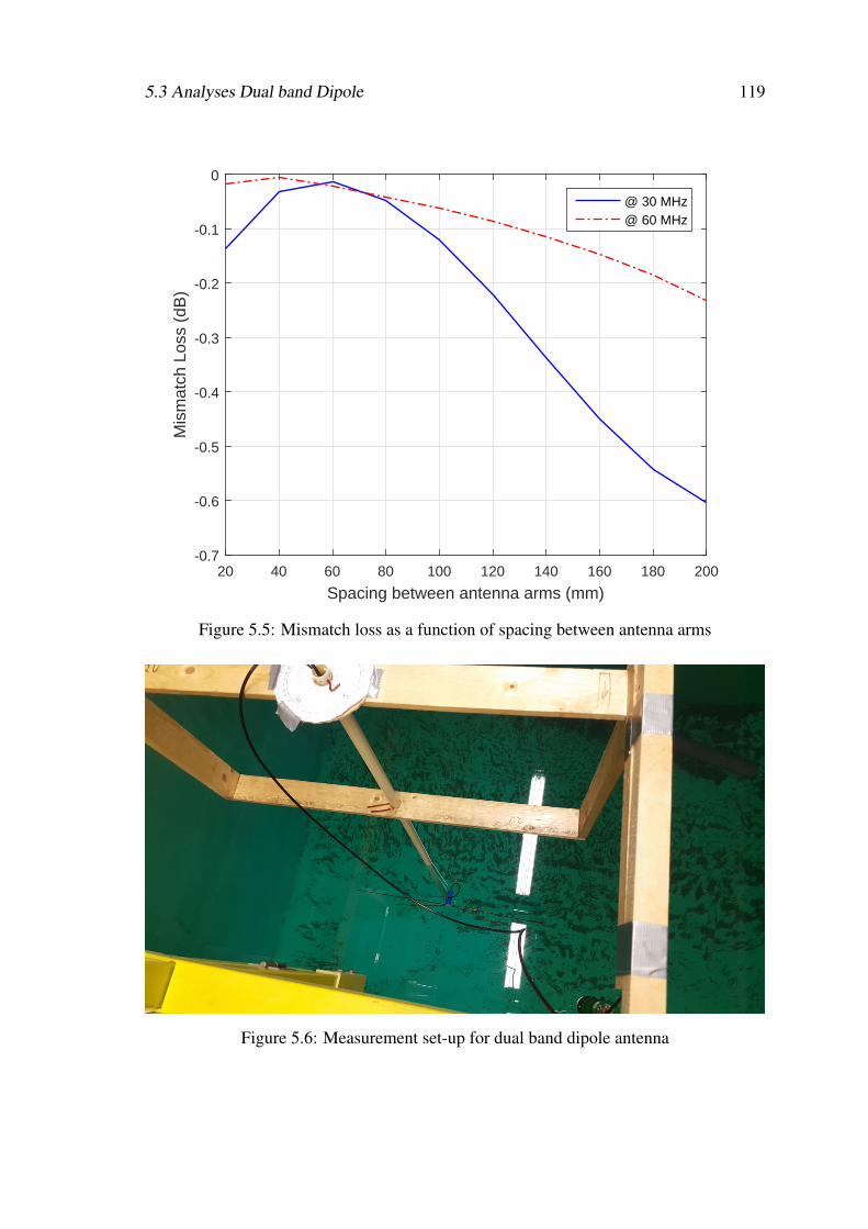
5.3 Analyses Dual band Dipole 119
20 40 60 80 100 120 140 160 180 200
Spacing between antenna arms (mm)
-0.7
-0.6
-0.5
-0.4
-0.3
-0.2
-0.1
0M
ism
atch
Los
s (d
B)
@ 30 MHz@ 60 MHz
Figure 5.5: Mismatch loss as a function of spacing between antenna arms
Figure 5.6: Measurement set-up for dual band dipole antenna
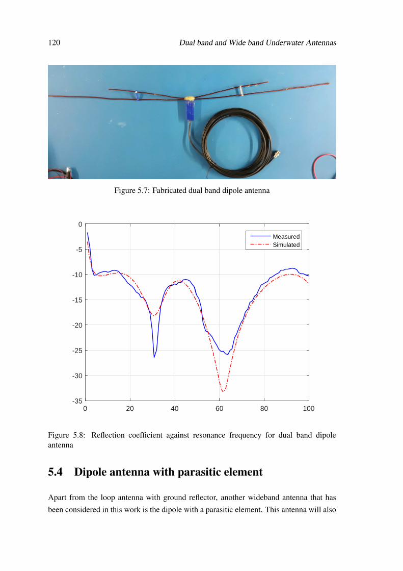
120 Dual band and Wide band Underwater Antennas
Figure 5.7: Fabricated dual band dipole antenna
0 20 40 60 80 100-35
-30
-25
-20
-15
-10
-5
0
MeasuredSimulated
Figure 5.8: Reflection coefficient against resonance frequency for dual band dipoleantenna
5.4 Dipole antenna with parasitic element
Apart from the loop antenna with ground reflector, another wideband antenna that hasbeen considered in this work is the dipole with a parasitic element. This antenna will also
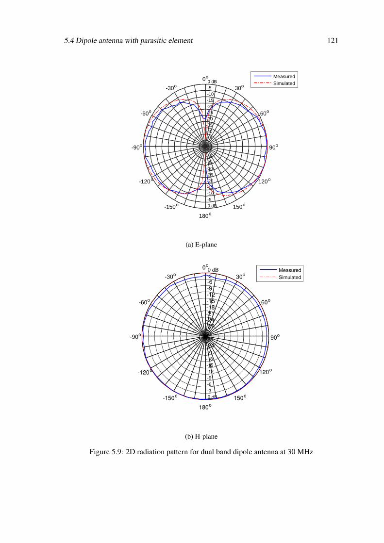
5.4 Dipole antenna with parasitic element 121
-45
-45
-40
-40
-35
-35
-30
-30
-25
-25
-20
-20
-15
-15
-10
-10
-5
-5
0 dB
0 dB
90o
60o
30o0o
-30o
-60o
-90o
-120o
-150o
180o150o
120o
MeasuredSimulated
(a) E-plane
-27
-27
-24
-24
-21
-21
-18
-18
-15
-15
-12
-12
-9
-9
-6
-6
-3
-3
0 dB
0 dB
90o
60o
30o
0o
-30o
-60o
-90o
-120o
-150o
180o
150o
120o
Measured
Simulated
(b) H-plane
Figure 5.9: 2D radiation pattern for dual band dipole antenna at 30 MHz
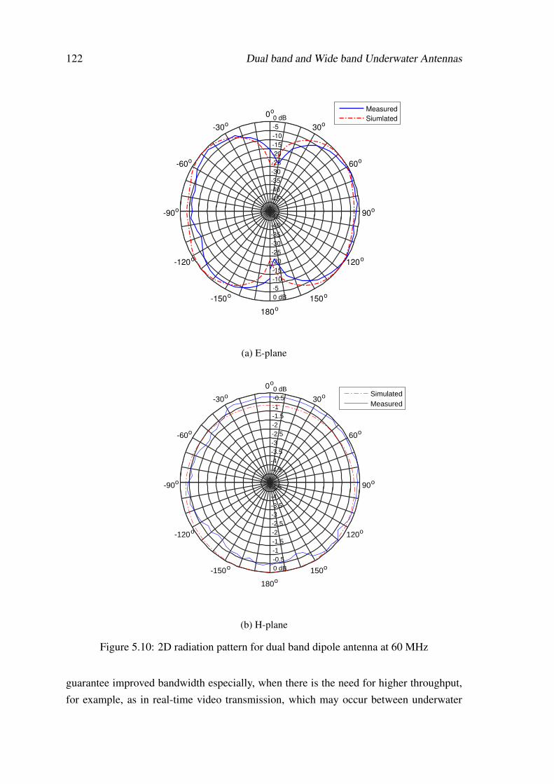
122 Dual band and Wide band Underwater Antennas
-45
-45
-40
-40
-35
-35
-30
-30
-25
-25
-20
-20
-15
-15
-10
-10
-5
-5
0 dB
0 dB
90o
60o
30o
0o
-30o
-60o
-90o
-120o
-150o
180o
150o
120o
Measured
Siumlated
(a) E-plane
-4.5
-4.5
-4
-4
-3.5
-3.5
-3
-3
-2.5
-2.5
-2
-2
-1.5
-1.5
-1
-1
-0.5
-0.5
0 dB
0 dB
90o
60o
30o
0o
-30o
-60o
-90o
-120o
-150o
180o
150o
120o
SimulatedMeasured
(b) H-plane
Figure 5.10: 2D radiation pattern for dual band dipole antenna at 60 MHz
guarantee improved bandwidth especially, when there is the need for higher throughput,for example, as in real-time video transmission, which may occur between underwater
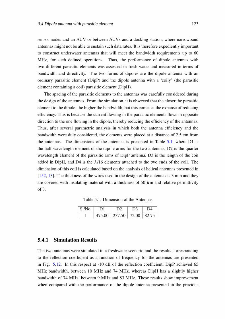
5.4 Dipole antenna with parasitic element 123
sensor nodes and an AUV or between AUVs and a docking station, where narrowbandantennas might not be able to sustain such data rates. It is therefore expediently importantto construct underwater antennas that will meet the bandwidth requirements up to 60MHz, for such defined operations. Thus, the performance of dipole antennas withtwo different parasitic elements was assessed in fresh water and measured in terms ofbandwidth and directivity. The two forms of dipoles are the dipole antenna with anordinary parasitic element (DipP) and the dipole antenna with a ‘coily’ (the parasiticelement containing a coil) parasitic element (DipH).
The spacing of the parasitic elements to the antennas was carefully considered duringthe design of the antennas. From the simulation, it is observed that the closer the parasiticelement to the dipole, the higher the bandwidth, but this comes at the expense of reducingefficiency. This is because the current flowing in the parasitic elements flows in oppositedirection to the one flowing in the dipole, thereby reducing the efficiency of the antennas.Thus, after several parametric analysis in which both the antenna efficiency and thebandwidth were duly considered, the elements were placed at a distance of 2.5 cm fromthe antennas. The dimensions of the antennas is presented in Table 5.1, where D1 isthe half wavelength element of the dipole arms for the two antennas, D2 is the quarterwavelength element of the parasitic arms of DipP antenna, D3 is the length of the coiladded in DipH, and D4 is the λ /16 elements attached to the two ends of the coil. Thedimension of this coil is calculated based on the analysis of helical antennas presented in[152, 13]. The thickness of the wires used in the design of the antennas is 3 mm and theyare covered with insulating material with a thickness of 50 µm and relative permittivityof 3.
Table 5.1: Dimension of the Antennas
S /No. D1 D2 D3 D41 475.00 237.50 72.00 82.75
5.4.1 Simulation Results
The two antennas were simulated in a freshwater scenario and the results correspondingto the reflection coefficient as a function of frequency for the antennas are presentedin Fig. 5.12. In this respect at -10 dB of the reflection coefficient, DipP achieved 65MHz bandwidth, between 10 MHz and 74 MHz, whereas DipH has a slightly higherbandwidth of 74 MHz, between 9 MHz and 83 MHz. These results show improvementwhen compared with the performance of the dipole antenna presented in the previous
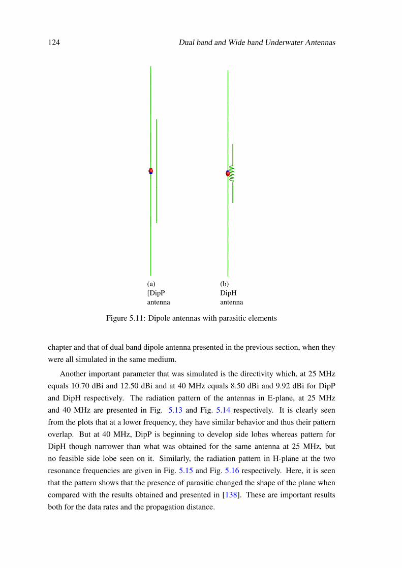
124 Dual band and Wide band Underwater Antennas
(a)[DipPantenna
(b)DipHantenna
Figure 5.11: Dipole antennas with parasitic elements
chapter and that of dual band dipole antenna presented in the previous section, when theywere all simulated in the same medium.
Another important parameter that was simulated is the directivity which, at 25 MHzequals 10.70 dBi and 12.50 dBi and at 40 MHz equals 8.50 dBi and 9.92 dBi for DipPand DipH respectively. The radiation pattern of the antennas in E-plane, at 25 MHzand 40 MHz are presented in Fig. 5.13 and Fig. 5.14 respectively. It is clearly seenfrom the plots that at a lower frequency, they have similar behavior and thus their patternoverlap. But at 40 MHz, DipP is beginning to develop side lobes whereas pattern forDipH though narrower than what was obtained for the same antenna at 25 MHz, butno feasible side lobe seen on it. Similarly, the radiation pattern in H-plane at the tworesonance frequencies are given in Fig. 5.15 and Fig. 5.16 respectively. Here, it is seenthat the pattern shows that the presence of parasitic changed the shape of the plane whencompared with the results obtained and presented in [138]. These are important resultsboth for the data rates and the propagation distance.
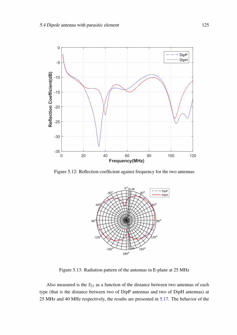
5.4 Dipole antenna with parasitic element 125
0 20 40 60 80 100 120
Frequency(MHz)
-35
-30
-25
-20
-15
-10
-5
0R
efl
ecti
on
Co
eff
icie
nt(
dB
)DipP
DipH
Figure 5.12: Reflection coefficient against frequency for the two antennas
-90
-90
-85
-85
-80
-80
-75
-75
-70
-70
-65
-65
-60
-60
-55
-55
-50
-50
-45 dB
-45 dB
90o
60o
30o0o
-30o
-60o
-90o
-120o
-150o
180o150o
120o
DipPDipH
Figure 5.13: Radiation pattern of the antennas in E-plane at 25 MHz
Also measured is the S21 as a function of the distance between two antennas of eachtype (that is the distance between two of DipP antennas and two of DipH antennas) at25 MHz and 40 MHz respectively, the results are presented in 5.17. The behavior of the
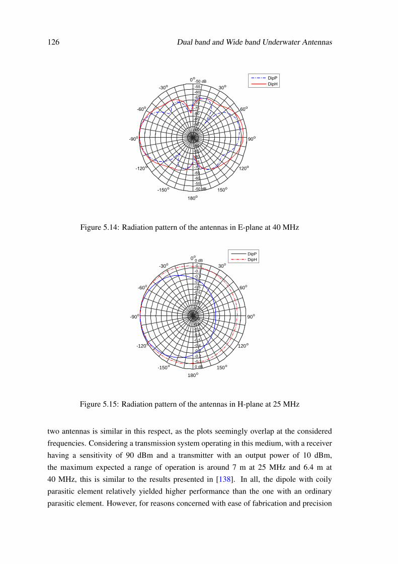
126 Dual band and Wide band Underwater Antennas
-95
-95
-90
-90
-85
-85
-80
-80
-75
-75
-70
-70
-65
-65
-60
-60
-55
-55
-50 dB
-50 dB
90o
60o
30o
0o
-30o
-60o
-90o
-120o
-150o
180o
150o
120o
DipP
DipH
Figure 5.14: Radiation pattern of the antennas in E-plane at 40 MHz
-0.9
-0.9
-0.8
-0.8
-0.7
-0.7
-0.6
-0.6
-0.5
-0.5
-0.4
-0.4
-0.3
-0.3
-0.2
-0.2
-0.1
-0.1
0 dB
0 dB
90o
60o
30o0o
-30o
-60o
-90o
-120o
-150o
180o150o
120o
DipPDipH
Figure 5.15: Radiation pattern of the antennas in H-plane at 25 MHz
two antennas is similar in this respect, as the plots seemingly overlap at the consideredfrequencies. Considering a transmission system operating in this medium, with a receiverhaving a sensitivity of 90 dBm and a transmitter with an output power of 10 dBm,the maximum expected a range of operation is around 7 m at 25 MHz and 6.4 m at40 MHz, this is similar to the results presented in [138]. In all, the dipole with coilyparasitic element relatively yielded higher performance than the one with an ordinaryparasitic element. However, for reasons concerned with ease of fabrication and precision
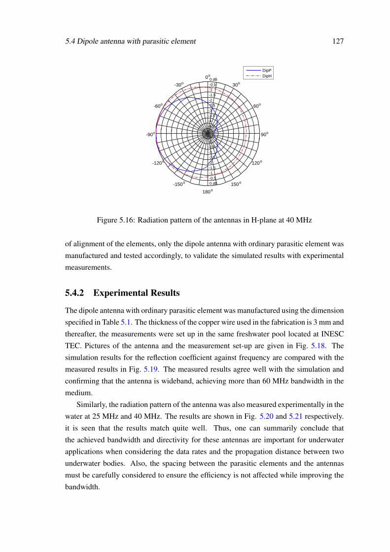
5.4 Dipole antenna with parasitic element 127
-4.5
-4.5
-4
-4
-3.5
-3.5
-3
-3
-2.5
-2.5
-2
-2
-1.5
-1.5
-1
-1
-0.5
-0.5
0 dB
0 dB
90o
60o
30o0o
-30o
-60o
-90o
-120o
-150o
180o150o
120o
DipPDipH
Figure 5.16: Radiation pattern of the antennas in H-plane at 40 MHz
of alignment of the elements, only the dipole antenna with ordinary parasitic element wasmanufactured and tested accordingly, to validate the simulated results with experimentalmeasurements.
5.4.2 Experimental Results
The dipole antenna with ordinary parasitic element was manufactured using the dimensionspecified in Table 5.1. The thickness of the copper wire used in the fabrication is 3 mm andthereafter, the measurements were set up in the same freshwater pool located at INESCTEC. Pictures of the antenna and the measurement set-up are given in Fig. 5.18. Thesimulation results for the reflection coefficient against frequency are compared with themeasured results in Fig. 5.19. The measured results agree well with the simulation andconfirming that the antenna is wideband, achieving more than 60 MHz bandwidth in themedium.
Similarly, the radiation pattern of the antenna was also measured experimentally in thewater at 25 MHz and 40 MHz. The results are shown in Fig. 5.20 and 5.21 respectively.it is seen that the results match quite well. Thus, one can summarily conclude thatthe achieved bandwidth and directivity for these antennas are important for underwaterapplications when considering the data rates and the propagation distance between twounderwater bodies. Also, the spacing between the parasitic elements and the antennasmust be carefully considered to ensure the efficiency is not affected while improving thebandwidth.
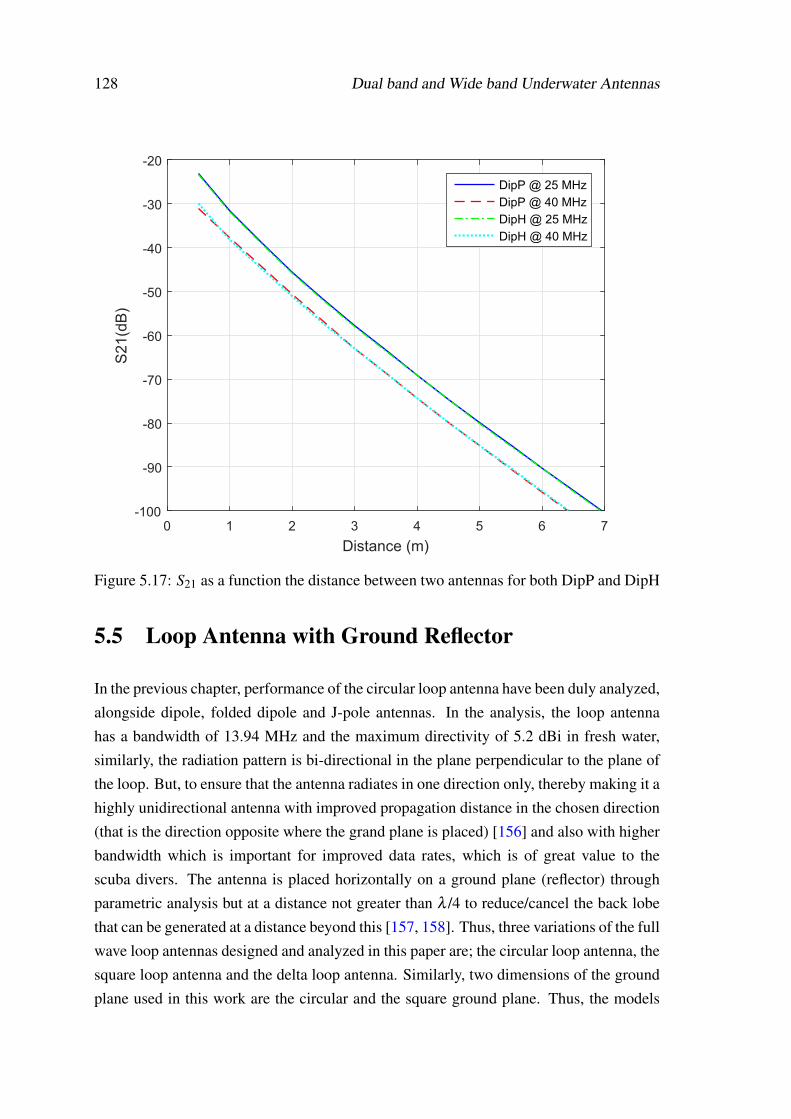
128 Dual band and Wide band Underwater Antennas
0 1 2 3 4 5 6 7
Distance (m)
-100
-90
-80
-70
-60
-50
-40
-30
-20
S21(d
B)
DipP @ 25 MHz
DipP @ 40 MHz
DipH @ 25 MHz
DipH @ 40 MHz
Figure 5.17: S21 as a function the distance between two antennas for both DipP and DipH
5.5 Loop Antenna with Ground Reflector
In the previous chapter, performance of the circular loop antenna have been duly analyzed,alongside dipole, folded dipole and J-pole antennas. In the analysis, the loop antennahas a bandwidth of 13.94 MHz and the maximum directivity of 5.2 dBi in fresh water,similarly, the radiation pattern is bi-directional in the plane perpendicular to the plane ofthe loop. But, to ensure that the antenna radiates in one direction only, thereby making it ahighly unidirectional antenna with improved propagation distance in the chosen direction(that is the direction opposite where the grand plane is placed) [156] and also with higherbandwidth which is important for improved data rates, which is of great value to thescuba divers. The antenna is placed horizontally on a ground plane (reflector) throughparametric analysis but at a distance not greater than λ /4 to reduce/cancel the back lobethat can be generated at a distance beyond this [157, 158]. Thus, three variations of the fullwave loop antennas designed and analyzed in this paper are; the circular loop antenna, thesquare loop antenna and the delta loop antenna. Similarly, two dimensions of the groundplane used in this work are the circular and the square ground plane. Thus, the models
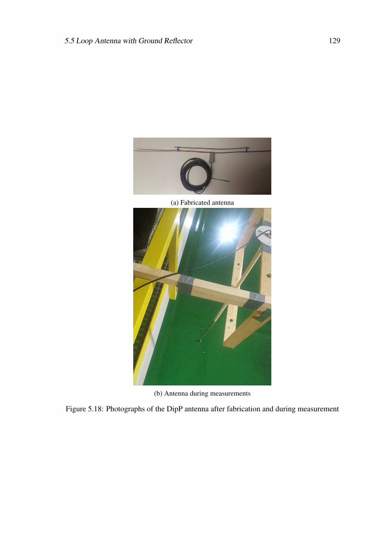
5.5 Loop Antenna with Ground Reflector 129
(a) Fabricated antenna
(b) Antenna during measurements
Figure 5.18: Photographs of the DipP antenna after fabrication and during measurement
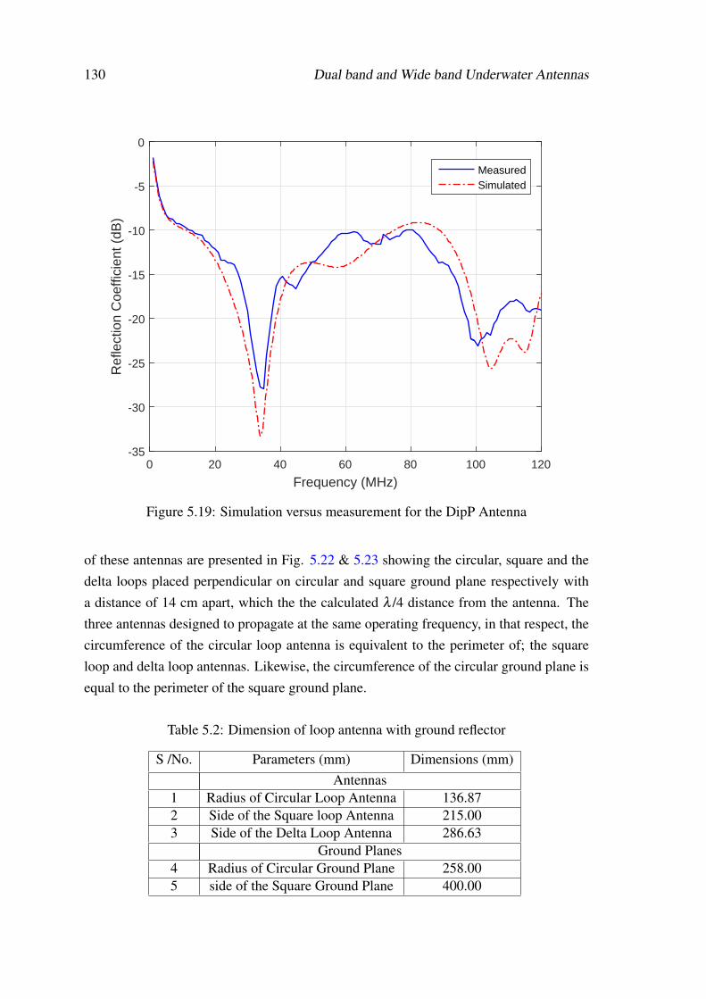
130 Dual band and Wide band Underwater Antennas
0 20 40 60 80 100 120
Frequency (MHz)
-35
-30
-25
-20
-15
-10
-5
0
Ref
lect
ion
Coe
ffici
ent (
dB)
MeasuredSimulated
Figure 5.19: Simulation versus measurement for the DipP Antenna
of these antennas are presented in Fig. 5.22 & 5.23 showing the circular, square and thedelta loops placed perpendicular on circular and square ground plane respectively witha distance of 14 cm apart, which the the calculated λ /4 distance from the antenna. Thethree antennas designed to propagate at the same operating frequency, in that respect, thecircumference of the circular loop antenna is equivalent to the perimeter of; the squareloop and delta loop antennas. Likewise, the circumference of the circular ground plane isequal to the perimeter of the square ground plane.
Table 5.2: Dimension of loop antenna with ground reflector
S /No. Parameters (mm) Dimensions (mm)Antennas
1 Radius of Circular Loop Antenna 136.872 Side of the Square loop Antenna 215.003 Side of the Delta Loop Antenna 286.63
Ground Planes4 Radius of Circular Ground Plane 258.005 side of the Square Ground Plane 400.00
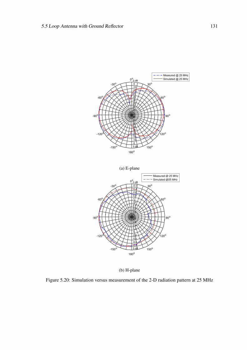
5.5 Loop Antenna with Ground Reflector 131
-45
-45
-40
-40
-35
-35
-30
-30
-25
-25
-20
-20
-15
-15
-10
-10
-5
-5
0 dB
0 dB
90o
60o
30o
0o
-30o
-60o
-90o
-120o
-150o
180o
150o
120o
Measured @ 25 MHz
Simulated @ 25 MHz
(a) E-plane
-1.8
-1.8
-1.6
-1.6
-1.4
-1.4
-1.2
-1.2
-1
-1
-0.8
-0.8
-0.6
-0.6
-0.4
-0.4
-0.2
-0.2
0 dB
0 dB
90o
60o
30o
0o
-30o
-60o
-90o
-120o
-150o
180o
150o
120o
Measured @ 25 MHz
Simulated @25 MHz
(b) H-plane
Figure 5.20: Simulation versus measurement of the 2-D radiation pattern at 25 MHz
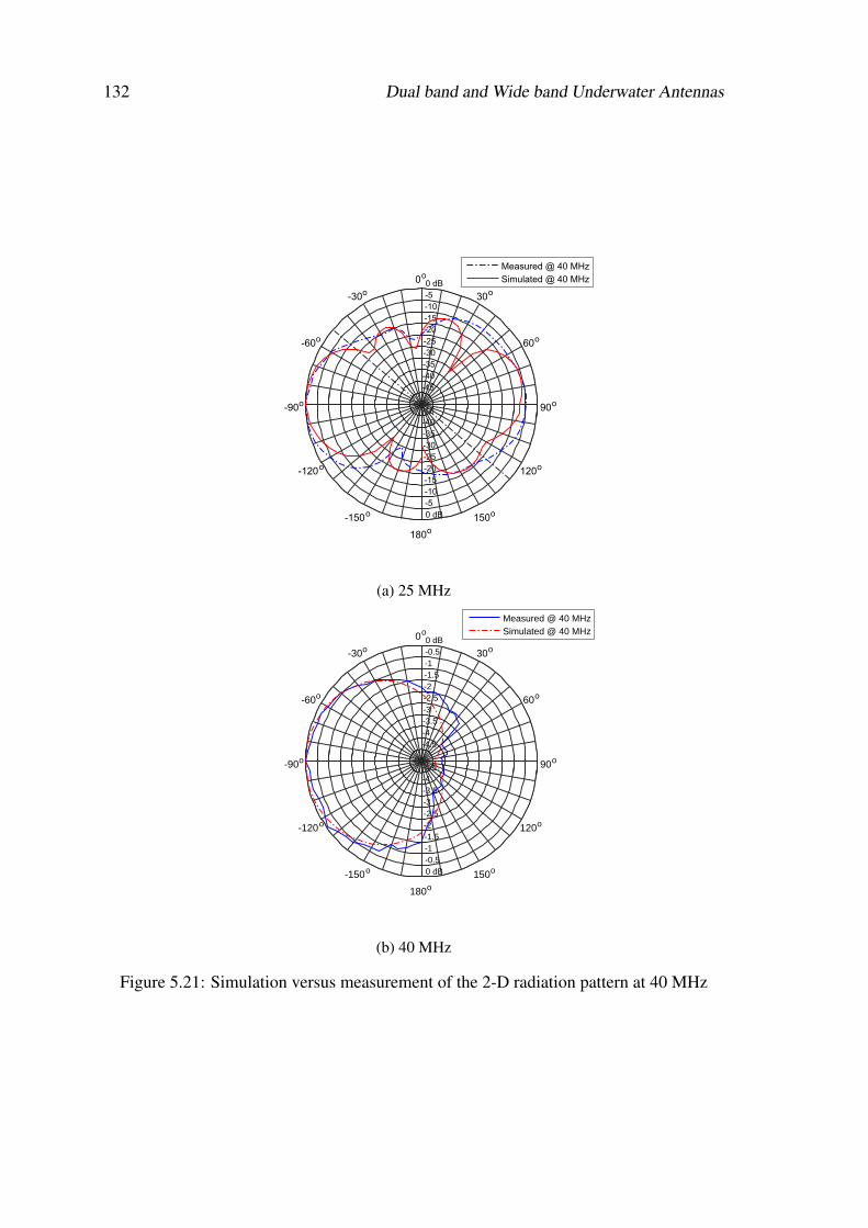
132 Dual band and Wide band Underwater Antennas
-45
-45
-40
-40
-35
-35
-30
-30
-25
-25
-20
-20
-15
-15
-10
-10
-5
-5
0 dB
0 dB
90o
60o
30o
0o
-30o
-60o
-90o
-120o
-150o
180o
150o
120o
Measured @ 40 MHz
Simulated @ 40 MHz
(a) 25 MHz
-4.5
-4.5
-4
-4
-3.5
-3.5
-3
-3
-2.5
-2.5
-2
-2
-1.5
-1.5
-1
-1
-0.5
-0.5
0 dB
0 dB
90o
60o
30o
0o
-30o
-60o
-90o
-120o
-150o
180o
150o
120o
Measured @ 40 MHzSimulated @ 40 MHz
(b) 40 MHz
Figure 5.21: Simulation versus measurement of the 2-D radiation pattern at 40 MHz
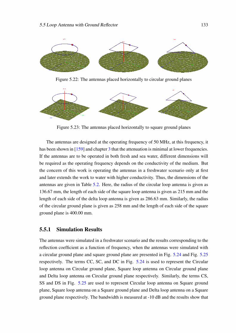
5.5 Loop Antenna with Ground Reflector 133
Figure 5.22: The antennas placed horizontally to circular ground planes
Figure 5.23: The antennas placed horizontally to square ground planes
The antennas are designed at the operating frequency of 50 MHz, at this frequency, ithas been shown in [159] and chapter 3 that the attenuation is minimal at lower frequencies.If the antennas are to be operated in both fresh and sea water, different dimensions willbe required as the operating frequency depends on the conductivity of the medium. Butthe concern of this work is operating the antennas in a freshwater scenario only at firstand later extends the work to water with higher conductivity. Thus, the dimensions of theantennas are given in Table 5.2. Here, the radius of the circular loop antenna is given as136.67 mm, the length of each side of the square loop antenna is given as 215 mm and thelength of each side of the delta loop antenna is given as 286.63 mm. Similarly, the radiusof the circular ground plane is given as 258 mm and the length of each side of the squareground plane is 400.00 mm.
5.5.1 Simulation Results
The antennas were simulated in a freshwater scenario and the results corresponding to thereflection coefficient as a function of frequency, when the antennas were simulated witha circular ground plane and square ground plane are presented in Fig. 5.24 and Fig. 5.25respectively. The terms CC, SC, and DC in Fig. 5.24 is used to represent the Circularloop antenna on Circular ground plane, Square loop antenna on Circular ground planeand Delta loop antenna on Circular ground plane respectively. Similarly, the terms CS,SS and DS in Fig. 5.25 are used to represent Circular loop antenna on Square groundplane, Square loop antenna on a Square ground plane and Delta loop antenna on a Squareground plane respectively. The bandwidth is measured at -10 dB and the results show that
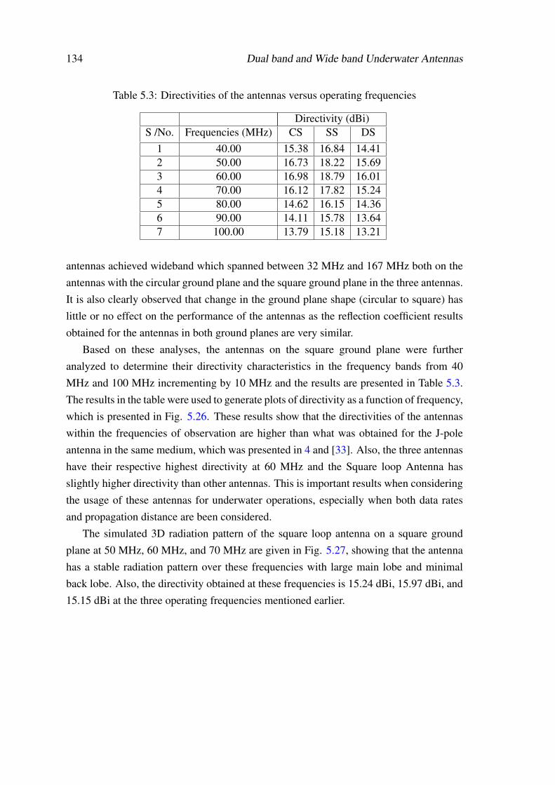
134 Dual band and Wide band Underwater Antennas
Table 5.3: Directivities of the antennas versus operating frequencies
Directivity (dBi)S /No. Frequencies (MHz) CS SS DS
1 40.00 15.38 16.84 14.412 50.00 16.73 18.22 15.693 60.00 16.98 18.79 16.014 70.00 16.12 17.82 15.245 80.00 14.62 16.15 14.366 90.00 14.11 15.78 13.647 100.00 13.79 15.18 13.21
antennas achieved wideband which spanned between 32 MHz and 167 MHz both on theantennas with the circular ground plane and the square ground plane in the three antennas.It is also clearly observed that change in the ground plane shape (circular to square) haslittle or no effect on the performance of the antennas as the reflection coefficient resultsobtained for the antennas in both ground planes are very similar.
Based on these analyses, the antennas on the square ground plane were furtheranalyzed to determine their directivity characteristics in the frequency bands from 40MHz and 100 MHz incrementing by 10 MHz and the results are presented in Table 5.3.The results in the table were used to generate plots of directivity as a function of frequency,which is presented in Fig. 5.26. These results show that the directivities of the antennaswithin the frequencies of observation are higher than what was obtained for the J-poleantenna in the same medium, which was presented in 4 and [33]. Also, the three antennashave their respective highest directivity at 60 MHz and the Square loop Antenna hasslightly higher directivity than other antennas. This is important results when consideringthe usage of these antennas for underwater operations, especially when both data ratesand propagation distance are been considered.
The simulated 3D radiation pattern of the square loop antenna on a square groundplane at 50 MHz, 60 MHz, and 70 MHz are given in Fig. 5.27, showing that the antennahas a stable radiation pattern over these frequencies with large main lobe and minimalback lobe. Also, the directivity obtained at these frequencies is 15.24 dBi, 15.97 dBi, and15.15 dBi at the three operating frequencies mentioned earlier.
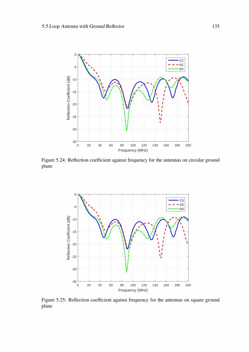
5.5 Loop Antenna with Ground Reflector 135
0 20 40 60 80 100 120 140 160 180 200
Frequency (MHz)
-35
-30
-25
-20
-15
-10
-5
0
Ref
lect
ion
Coe
ffici
ent (
dB)
CCSCDC
Figure 5.24: Reflection coefficient against frequency for the antennas on circular groundplane
0 20 40 60 80 100 120 140 160 180 200
Frequency (MHz)
-35
-30
-25
-20
-15
-10
-5
0
Ref
lect
ion
Coe
ffici
ent (
dB)
CSSSDS
Figure 5.25: Reflection coefficient against frequency for the antennas on square groundplane
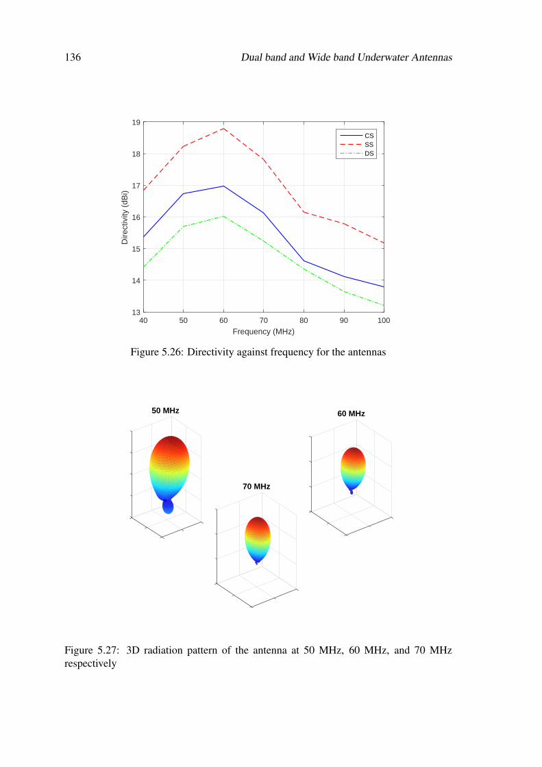
136 Dual band and Wide band Underwater Antennas
40 50 60 70 80 90 100
Frequency (MHz)
13
14
15
16
17
18
19D
irect
ivity
(dB
i)
CSSSDS
Figure 5.26: Directivity against frequency for the antennas
50 MHz 60 MHz
70 MHz
Figure 5.27: 3D radiation pattern of the antenna at 50 MHz, 60 MHz, and 70 MHzrespectively
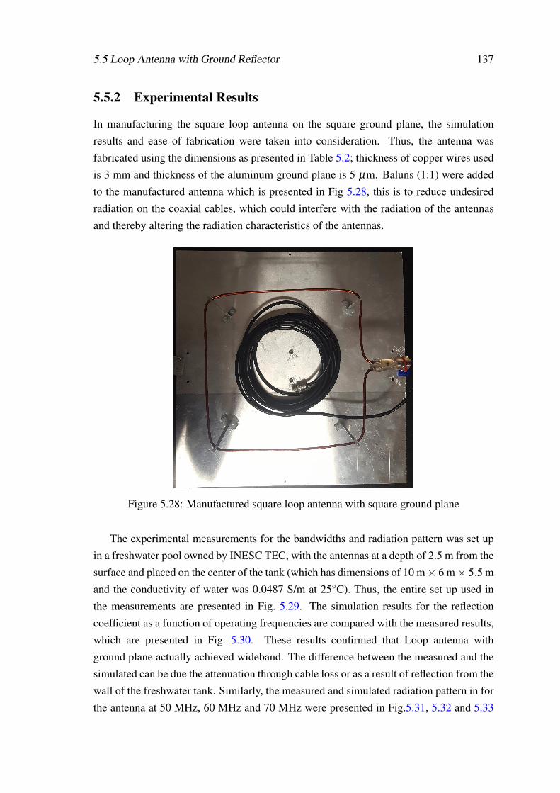
5.5 Loop Antenna with Ground Reflector 137
5.5.2 Experimental Results
In manufacturing the square loop antenna on the square ground plane, the simulationresults and ease of fabrication were taken into consideration. Thus, the antenna wasfabricated using the dimensions as presented in Table 5.2; thickness of copper wires usedis 3 mm and thickness of the aluminum ground plane is 5 µm. Baluns (1:1) were addedto the manufactured antenna which is presented in Fig 5.28, this is to reduce undesiredradiation on the coaxial cables, which could interfere with the radiation of the antennasand thereby altering the radiation characteristics of the antennas.
Figure 5.28: Manufactured square loop antenna with square ground plane
The experimental measurements for the bandwidths and radiation pattern was set upin a freshwater pool owned by INESC TEC, with the antennas at a depth of 2.5 m from thesurface and placed on the center of the tank (which has dimensions of 10 m× 6 m× 5.5 mand the conductivity of water was 0.0487 S/m at 25C). Thus, the entire set up used inthe measurements are presented in Fig. 5.29. The simulation results for the reflectioncoefficient as a function of operating frequencies are compared with the measured results,which are presented in Fig. 5.30. These results confirmed that Loop antenna withground plane actually achieved wideband. The difference between the measured and thesimulated can be due the attenuation through cable loss or as a result of reflection from thewall of the freshwater tank. Similarly, the measured and simulated radiation pattern in forthe antenna at 50 MHz, 60 MHz and 70 MHz were presented in Fig.5.31, 5.32 and 5.33
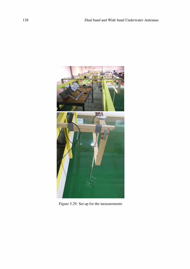
138 Dual band and Wide band Underwater Antennas
Figure 5.29: Set up for the measurements
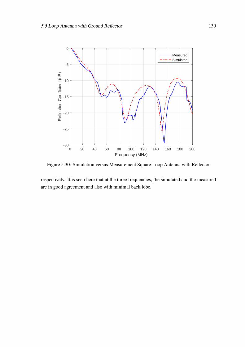
5.5 Loop Antenna with Ground Reflector 139
0 20 40 60 80 100 120 140 160 180 200
Frequency (MHz)
-30
-25
-20
-15
-10
-5
0
Ref
lect
ion
Coe
ffici
ent (
dB)
MeasuredSimulated
Figure 5.30: Simulation versus Measurement Square Loop Antenna with Reflector
respectively. It is seen here that at the three frequencies, the simulated and the measuredare in good agreement and also with minimal back lobe.
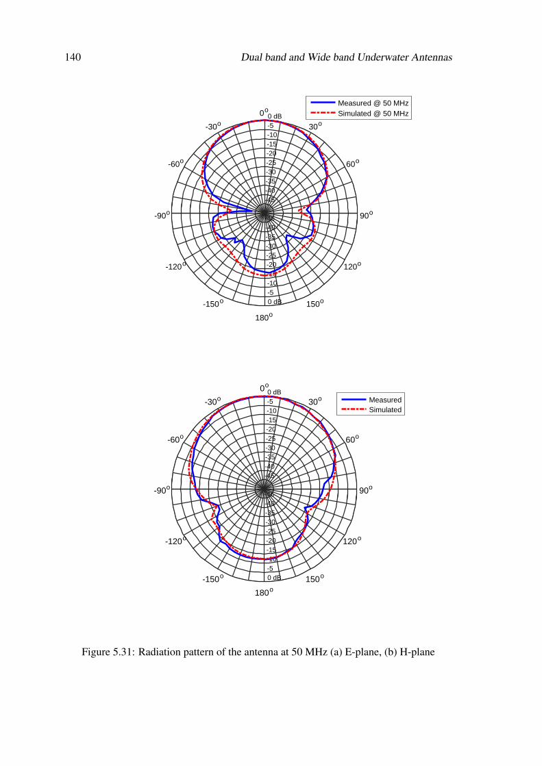
140 Dual band and Wide band Underwater Antennas
-45
-45
-40
-40
-35
-35
-30
-30
-25
-25
-20
-20
-15
-15
-10
-10
-5
-5
0 dB
0 dB
90o
60o
30o
0o
-30o
-60o
-90o
-120o
-150o
180o
150o
120o
Measured @ 50 MHzSimulated @ 50 MHz
-45
-45
-40
-40
-35
-35
-30
-30
-25
-25
-20
-20
-15
-15
-10
-10
-5
-5
0 dB
0 dB
90o
60o
30o0o
-30o
-60o
-90o
-120o
-150o
180o150o
120o
MeasuredSimulated
Figure 5.31: Radiation pattern of the antenna at 50 MHz (a) E-plane, (b) H-plane
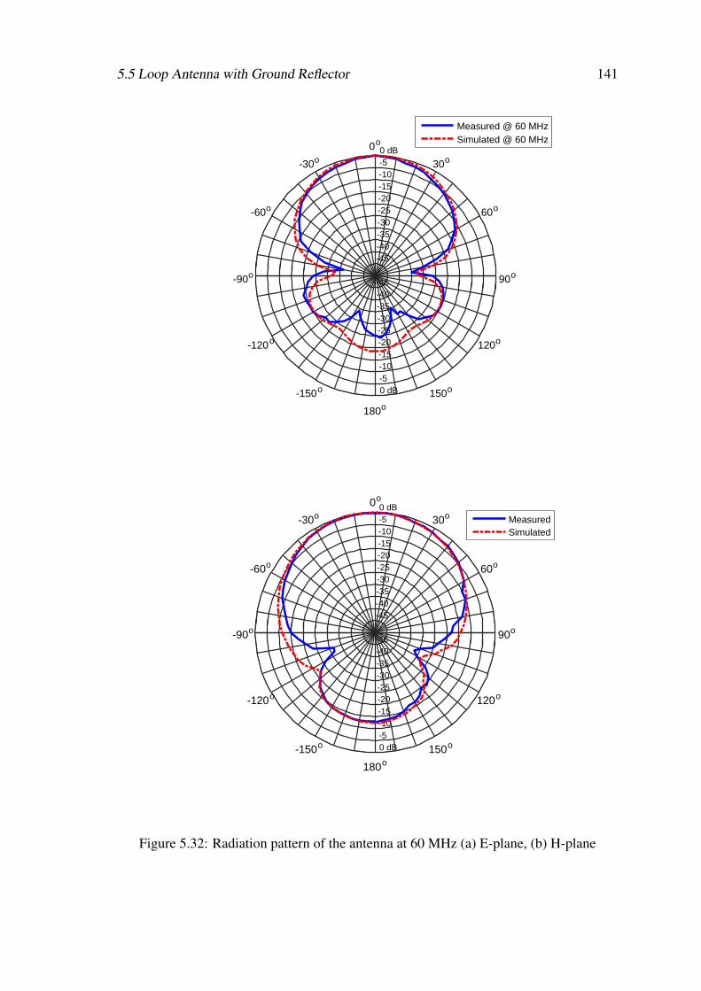
5.5 Loop Antenna with Ground Reflector 141
-45
-45
-40
-40
-35
-35
-30
-30
-25
-25
-20
-20
-15
-15
-10
-10
-5
-5
0 dB
0 dB
90o
60o
30o
0o
-30o
-60o
-90o
-120o
-150o
180o
150o
120o
Measured @ 60 MHzSimulated @ 60 MHz
-45
-45
-40
-40
-35
-35
-30
-30
-25
-25
-20
-20
-15
-15
-10
-10
-5
-5
0 dB
0 dB
90o
60o
30o0o
-30o
-60o
-90o
-120o
-150o
180o150o
120o
MeasuredSimulated
Figure 5.32: Radiation pattern of the antenna at 60 MHz (a) E-plane, (b) H-plane
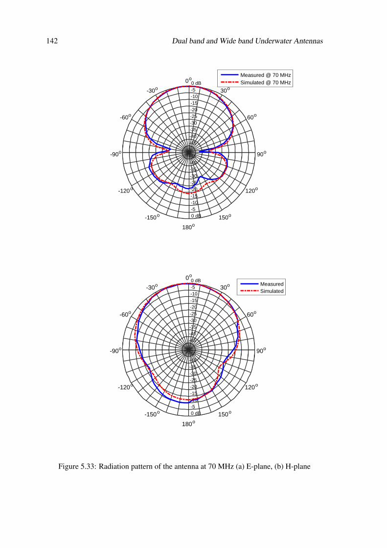
142 Dual band and Wide band Underwater Antennas
-45
-45
-40
-40
-35
-35
-30
-30
-25
-25
-20
-20
-15
-15
-10
-10
-5
-5
0 dB
0 dB
90o
60o
30o
0o
-30o
-60o
-90o
-120o
-150o
180o
150o
120o
Measured @ 70 MHzSimulated @ 70 MHz
-45
-45
-40
-40
-35
-35
-30
-30
-25
-25
-20
-20
-15
-15
-10
-10
-5
-5
0 dB
0 dB
90o
60o
30o0o
-30o
-60o
-90o
-120o
-150o
180o150o
120o
MeasuredSimulated
Figure 5.33: Radiation pattern of the antenna at 70 MHz (a) E-plane, (b) H-plane
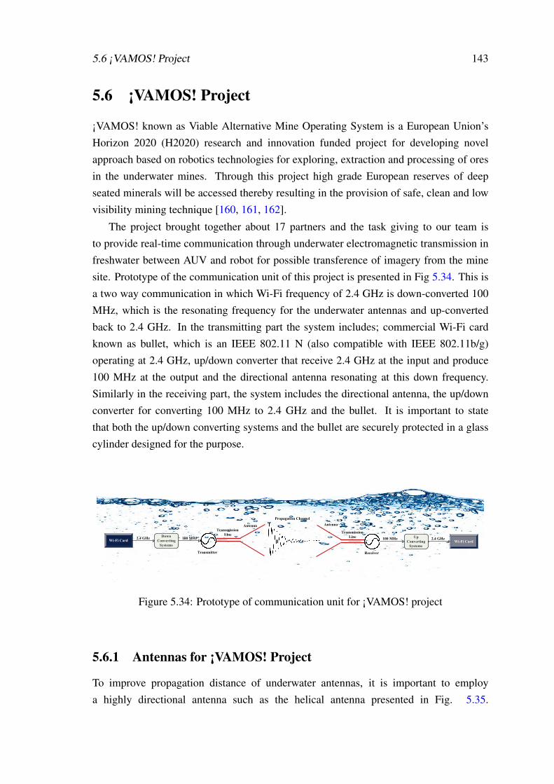
5.6 ¡VAMOS! Project 143
5.6 ¡VAMOS! Project
¡VAMOS! known as Viable Alternative Mine Operating System is a European Union’sHorizon 2020 (H2020) research and innovation funded project for developing novelapproach based on robotics technologies for exploring, extraction and processing of oresin the underwater mines. Through this project high grade European reserves of deepseated minerals will be accessed thereby resulting in the provision of safe, clean and lowvisibility mining technique [160, 161, 162].
The project brought together about 17 partners and the task giving to our team isto provide real-time communication through underwater electromagnetic transmission infreshwater between AUV and robot for possible transference of imagery from the minesite. Prototype of the communication unit of this project is presented in Fig 5.34. This isa two way communication in which Wi-Fi frequency of 2.4 GHz is down-converted 100MHz, which is the resonating frequency for the underwater antennas and up-convertedback to 2.4 GHz. In the transmitting part the system includes; commercial Wi-Fi cardknown as bullet, which is an IEEE 802.11 N (also compatible with IEEE 802.11b/g)operating at 2.4 GHz, up/down converter that receive 2.4 GHz at the input and produce100 MHz at the output and the directional antenna resonating at this down frequency.Similarly in the receiving part, the system includes the directional antenna, the up/downconverter for converting 100 MHz to 2.4 GHz and the bullet. It is important to statethat both the up/down converting systems and the bullet are securely protected in a glasscylinder designed for the purpose.
Propagation Channel
Antenna
Transmitter
Transmission Line
Antenna
Receiver
Transmission Line
Wi-Fi Card2.4 GHz Down
Converting Systems
100 MHzWi-Fi Card
2.4 GHzUp Converting
Systems
100 MHz
Figure 5.34: Prototype of communication unit for ¡VAMOS! project
5.6.1 Antennas for ¡VAMOS! Project
To improve propagation distance of underwater antennas, it is important to employa highly directional antenna such as the helical antenna presented in Fig. 5.35.
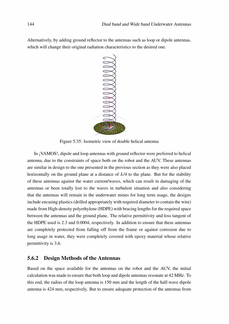
144 Dual band and Wide band Underwater Antennas
Alternatively, by adding ground reflector to the antennas such as loop or dipole antennas,which will change their original radiation characteristics to the desired one.
Figure 5.35: Isometric view of double helical antenna
In ¡VAMOS!, dipole and loop antennas with ground reflector were preferred to helicalantenna, due to the constraints of space both on the robot and the AUV. These antennasare similar in design to the one presented in the previous section as they were also placedhorizontally on the ground plane at a distance of λ /4 to the plane. But for the stabilityof these antennas against the water current/waves, which can result in damaging of theantennas or been totally lost to the waves in turbulent situation and also consideringthat the antennas will remain in the underwater mines for long term usage, the designsinclude encasing plastics (drilled appropriately with required diameter to contain the wire)made from High-density polyethylene (HDPE) with bracing lengths for the required spacebetween the antennas and the ground plane. The relative permittivity and loss tangent ofthe HDPE used is 2.3 and 0.0004, respectively. In addition to ensure that these antennasare completely protected from falling off from the frame or against corrosion due tolong usage in water, they were completely covered with epoxy material whose relativepermittivity is 3.6.
5.6.2 Design Methods of the Antennas
Based on the space available for the antennas on the robot and the AUV, the initialcalculation was made to ensure that both loop and dipole antennas resonate at 42 MHz. Tothis end, the radius of the loop antenna is 150 mm and the length of the half-wave dipoleantenna is 424 mm, respectively. But to ensure adequate protection of the antennas from
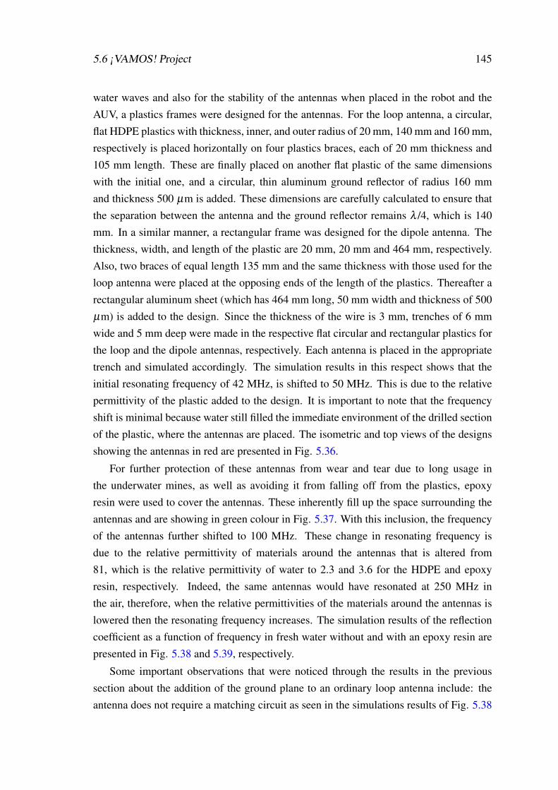
5.6 ¡VAMOS! Project 145
water waves and also for the stability of the antennas when placed in the robot and theAUV, a plastics frames were designed for the antennas. For the loop antenna, a circular,flat HDPE plastics with thickness, inner, and outer radius of 20 mm, 140 mm and 160 mm,respectively is placed horizontally on four plastics braces, each of 20 mm thickness and105 mm length. These are finally placed on another flat plastic of the same dimensionswith the initial one, and a circular, thin aluminum ground reflector of radius 160 mmand thickness 500 µm is added. These dimensions are carefully calculated to ensure thatthe separation between the antenna and the ground reflector remains λ /4, which is 140mm. In a similar manner, a rectangular frame was designed for the dipole antenna. Thethickness, width, and length of the plastic are 20 mm, 20 mm and 464 mm, respectively.Also, two braces of equal length 135 mm and the same thickness with those used for theloop antenna were placed at the opposing ends of the length of the plastics. Thereafter arectangular aluminum sheet (which has 464 mm long, 50 mm width and thickness of 500µm) is added to the design. Since the thickness of the wire is 3 mm, trenches of 6 mmwide and 5 mm deep were made in the respective flat circular and rectangular plastics forthe loop and the dipole antennas, respectively. Each antenna is placed in the appropriatetrench and simulated accordingly. The simulation results in this respect shows that theinitial resonating frequency of 42 MHz, is shifted to 50 MHz. This is due to the relativepermittivity of the plastic added to the design. It is important to note that the frequencyshift is minimal because water still filled the immediate environment of the drilled sectionof the plastic, where the antennas are placed. The isometric and top views of the designsshowing the antennas in red are presented in Fig. 5.36.
For further protection of these antennas from wear and tear due to long usage inthe underwater mines, as well as avoiding it from falling off from the plastics, epoxyresin were used to cover the antennas. These inherently fill up the space surrounding theantennas and are showing in green colour in Fig. 5.37. With this inclusion, the frequencyof the antennas further shifted to 100 MHz. These change in resonating frequency isdue to the relative permittivity of materials around the antennas that is altered from81, which is the relative permittivity of water to 2.3 and 3.6 for the HDPE and epoxyresin, respectively. Indeed, the same antennas would have resonated at 250 MHz inthe air, therefore, when the relative permittivities of the materials around the antennas islowered then the resonating frequency increases. The simulation results of the reflectioncoefficient as a function of frequency in fresh water without and with an epoxy resin arepresented in Fig. 5.38 and 5.39, respectively.
Some important observations that were noticed through the results in the previoussection about the addition of the ground plane to an ordinary loop antenna include: theantenna does not require a matching circuit as seen in the simulations results of Fig. 5.38
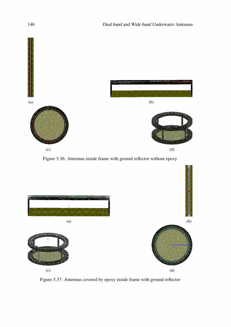
146 Dual band and Wide band Underwater Antennas
(a) (b)
(c) (d)
Figure 5.36: Antennas inside frame with ground reflector without epoxy
(a) (b)
(c) (d)
Figure 5.37: Antennas covered by epoxy inside frame with ground reflector
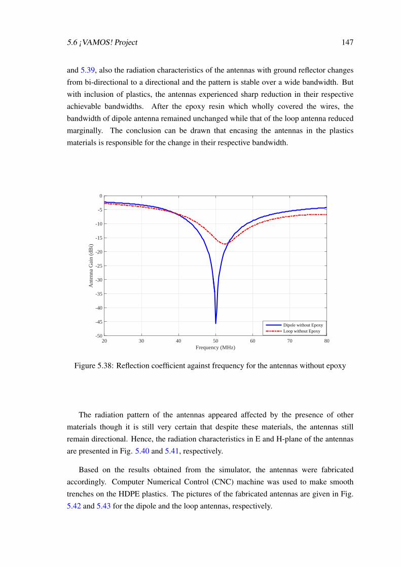
5.6 ¡VAMOS! Project 147
and 5.39, also the radiation characteristics of the antennas with ground reflector changesfrom bi-directional to a directional and the pattern is stable over a wide bandwidth. Butwith inclusion of plastics, the antennas experienced sharp reduction in their respectiveachievable bandwidths. After the epoxy resin which wholly covered the wires, thebandwidth of dipole antenna remained unchanged while that of the loop antenna reducedmarginally. The conclusion can be drawn that encasing the antennas in the plasticsmaterials is responsible for the change in their respective bandwidth.
20 30 40 50 60 70 80Frequency (MHz)
-50
-45
-40
-35
-30
-25
-20
-15
-10
-5
0
Ant
enna
Gai
n (d
Bi)
Dipole without EpoxyLoop without Epoxy
Figure 5.38: Reflection coefficient against frequency for the antennas without epoxy
The radiation pattern of the antennas appeared affected by the presence of othermaterials though it is still very certain that despite these materials, the antennas stillremain directional. Hence, the radiation characteristics in E and H-plane of the antennasare presented in Fig. 5.40 and 5.41, respectively.
Based on the results obtained from the simulator, the antennas were fabricatedaccordingly. Computer Numerical Control (CNC) machine was used to make smoothtrenches on the HDPE plastics. The pictures of the fabricated antennas are given in Fig.5.42 and 5.43 for the dipole and the loop antennas, respectively.
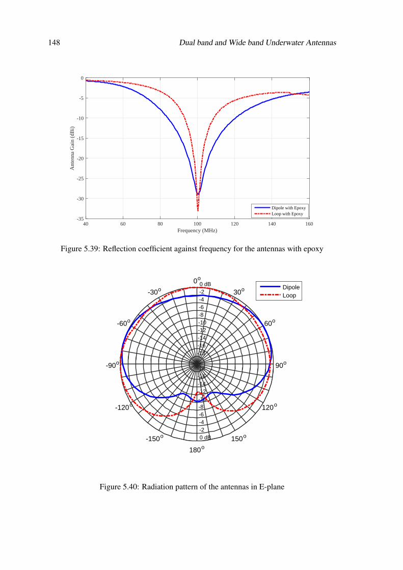
148 Dual band and Wide band Underwater Antennas
40 60 80 100 120 140 160Frequency (MHz)
-35
-30
-25
-20
-15
-10
-5
0A
nten
na G
ain
(dB
i)
Dipole with EpoxyLoop with Epoxy
Figure 5.39: Reflection coefficient against frequency for the antennas with epoxy
-18
-18
-16
-16
-14
-14
-12
-12
-10
-10
-8
-8
-6
-6
-4
-4
-2
-2
0 dB
0 dB
90o
60o
30o0o
-30o
-60o
-90o
-120o
-150o
180o150o
120o
DipoleLoop
Figure 5.40: Radiation pattern of the antennas in E-plane
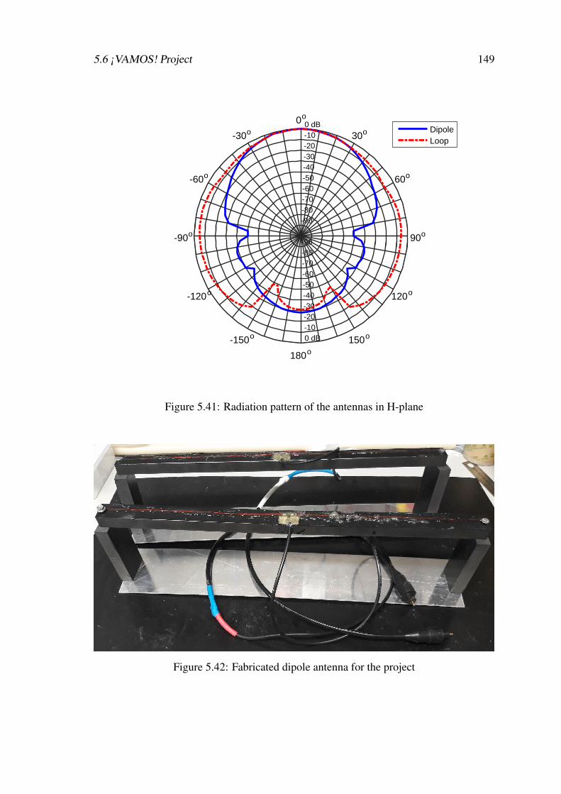
5.6 ¡VAMOS! Project 149
-90
-90
-80
-80
-70
-70
-60
-60
-50
-50
-40
-40
-30
-30
-20
-20
-10
-10
0 dB
0 dB
90o
60o
30o0o
-30o
-60o
-90o
-120o
-150o
180o150o
120o
DipoleLoop
Figure 5.41: Radiation pattern of the antennas in H-plane
Figure 5.42: Fabricated dipole antenna for the project
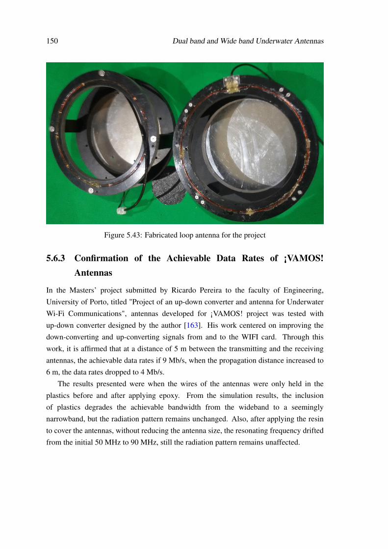
150 Dual band and Wide band Underwater Antennas
Figure 5.43: Fabricated loop antenna for the project
5.6.3 Confirmation of the Achievable Data Rates of ¡VAMOS!Antennas
In the Masters’ project submitted by Ricardo Pereira to the faculty of Engineering,University of Porto, titled "Project of an up-down converter and antenna for UnderwaterWi-Fi Communications", antennas developed for ¡VAMOS! project was tested withup-down converter designed by the author [163]. His work centered on improving thedown-converting and up-converting signals from and to the WIFI card. Through thiswork, it is affirmed that at a distance of 5 m between the transmitting and the receivingantennas, the achievable data rates if 9 Mb/s, when the propagation distance increased to6 m, the data rates dropped to 4 Mb/s.
The results presented were when the wires of the antennas were only held in theplastics before and after applying epoxy. From the simulation results, the inclusionof plastics degrades the achievable bandwidth from the wideband to a seeminglynarrowband, but the radiation pattern remains unchanged. Also, after applying the resinto cover the antennas, without reducing the antenna size, the resonating frequency driftedfrom the initial 50 MHz to 90 MHz, still the radiation pattern remains unaffected.
5.7 Friis Equation for Underwater Antennas 151
5.7 Friis Equation for Underwater Antennas
One of the fundamental equation in antenna technology is the Friis equation (Friisformula), which is used to calculate the received power when two antennas are separatedby a distance R > 2D2
λ. Once the gain of the antennas are known, then the received power
(Pr) can be calculated as presented in [10]:
Pr =PtGtGrλ
2
(4πd)2 , (5.1)
where Pt is the transmitted power, Gt is the gain of the transmitting antenna, Gr is thegain of the received antenna, and R = d is the distance between the transmitting and thereceiving antennas. The term ( λ
4πd )−2 is known as the free-space loss (FSL), which takes
into consideration losses due to spherical spreading of the energy by the antenna [13].This is written as:
FSL =
(4πd
λ
)2
. (5.2)
In free-space, this parameter is dependent on the wavelength and the distance betweenthe transmitting and the receiving antennas. However, in water electromagnetic spreadingis through a medium with conductivity and high permittivity, hence losses in water aredependent on the distance between the transmitter and the receiver, water itself and itsconductive level, which increases with the resonating frequency.
To that purpose the previous equation is modified, by replacing the wavelength λ with2π
βand the equation becomes:
FSL = (2dβ )2. (5.3)
In decibel, FSL is given as:
FSL = 20log10(2dβ ). (5.4)
For antennas that are wholly submerged in fresh or sea water, the path loss, Lp, equals theloss through the medium (water) which can be determined by considering equation 3.42in terms of its cosine functions as:
γ = ω
√µε ′ (1− cosδe)
2cosδe+ jω
√µε ′ (1+ cosδe)
2cosδem, (5.5)
152 Dual band and Wide band Underwater Antennas
Given that the attenuation constant is the real part of this equation, then path loss isgiven as:
Lp = 20. log10
(eαd)= 8.68αd. (5.6)
in linear form, this is given as
Lp = 10(8.68αd/10). (5.7)
Consequently, the Friis equation for underwater antenna communication with theinclusion of the attenuation through the medium is presented as:
Pr = PtGtGrLpFSL. (5.8)
Therefore, equation 5.8 will be used to determine the "gains" of underwater antennasand can also be the link budget for underwater communication systems, but this is notincluded in this thesis.
5.7.1 Realized Gains of Underwater Antennas
To determine the realized gain of underwater antennas from equation 5.8, the followingequivalents were used from the S-parameters
• Transmitted power Pt relative to the incident is measured by the mismatch lossthrough the system, hence
Pt = |1−S11|2; (5.9)
• Received power Pr is the modulus of transmission coefficient given as
Pr = |S21|2. (5.10)
Also, if the transmitting and the receiving antennas are of the same type (for instancetwo dipole antennas) and operating at the same frequency, then their respective gains arealso equal and equation 5.8 becomes
|S21|2 = |1−S11|2G2LpFSL, (5.11)
this can be rearranged to determine the realized gains as:
G =
√|S21|2
|1−S11|2.
1LP.FSL
, (5.12)
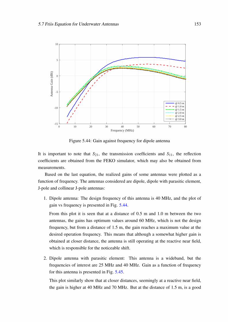
5.7 Friis Equation for Underwater Antennas 153
0 10 20 30 40 50 60 70 80
Frequency (MHz)
-15
-10
-5
0
5
10
Ant
enna
Gai
n (d
Bi)
@ 0.5 m@ 1.0 m@ 1.5 m@ 2.0 m@ 2.5 m@ 3.0 m
Figure 5.44: Gain against frequency for dipole antenna
It is important to note that S21, the transmission coefficients and S11, the reflectioncoefficients are obtained from the FEKO simulator, which may also be obtained frommeasurements.
Based on the last equation, the realized gains of some antennas were plotted as afunction of frequency. The antennas considered are dipole, dipole with parasitic element,J-pole and collinear J-pole antennas:
1. Dipole antenna: The design frequency of this antenna is 40 MHz, and the plot ofgain vs frequency is presented in Fig. 5.44.
From this plot it is seen that at a distance of 0.5 m and 1.0 m between the twoantennas, the gains has optimum values around 60 MHz, which is not the designfrequency, but from a distance of 1.5 m, the gain reaches a maximum value at thedesired operation frequency. This means that although a somewhat higher gain isobtained at closer distance, the antenna is still operating at the reactive near field,which is responsible for the noticeable shift.
2. Dipole antenna with parasitic element: This antenna is a wideband, but thefrequencies of interest are 25 MHz and 40 MHz. Gain as a function of frequencyfor this antenna is presented in Fig. 5.45.
This plot similarly show that at closer distances, seemingly at a reactive near field,the gain is higher at 40 MHz and 70 MHz. But at the distance of 1.5 m, is a good
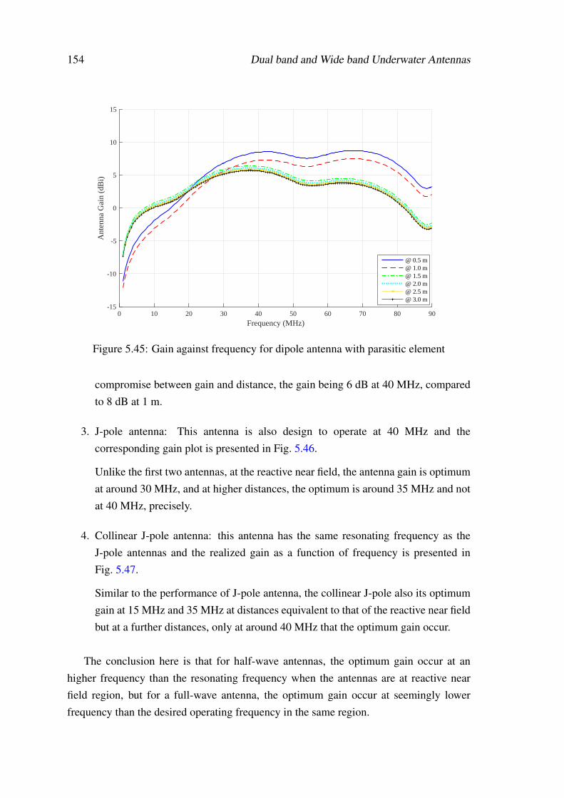
154 Dual band and Wide band Underwater Antennas
0 10 20 30 40 50 60 70 80 90
Frequency (MHz)
-15
-10
-5
0
5
10
15A
nten
na G
ain
(dB
i)
@ 0.5 m@ 1.0 m@ 1.5 m@ 2.0 m@ 2.5 m@ 3.0 m
Figure 5.45: Gain against frequency for dipole antenna with parasitic element
compromise between gain and distance, the gain being 6 dB at 40 MHz, comparedto 8 dB at 1 m.
3. J-pole antenna: This antenna is also design to operate at 40 MHz and thecorresponding gain plot is presented in Fig. 5.46.
Unlike the first two antennas, at the reactive near field, the antenna gain is optimumat around 30 MHz, and at higher distances, the optimum is around 35 MHz and notat 40 MHz, precisely.
4. Collinear J-pole antenna: this antenna has the same resonating frequency as theJ-pole antennas and the realized gain as a function of frequency is presented inFig. 5.47.
Similar to the performance of J-pole antenna, the collinear J-pole also its optimumgain at 15 MHz and 35 MHz at distances equivalent to that of the reactive near fieldbut at a further distances, only at around 40 MHz that the optimum gain occur.
The conclusion here is that for half-wave antennas, the optimum gain occur at anhigher frequency than the resonating frequency when the antennas are at reactive nearfield region, but for a full-wave antenna, the optimum gain occur at seemingly lowerfrequency than the desired operating frequency in the same region.
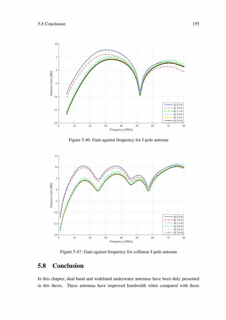
5.8 Conclusion 155
0 10 20 30 40 50 60 70 80
Frequency (MHz)
-20
-15
-10
-5
0
5
10
Ant
enna
Gai
n (d
Bi)
@ 0.5 m@ 1.0 m@ 1.5 m@ 2.0 m@ 2.5 m@ 3.0 m
Figure 5.46: Gain against frequency for J-pole antenna
0 10 20 30 40 50 60 70 80
Frequency (MHz)
-20
-15
-10
-5
0
5
10
15
Ant
enna
Gai
n (d
Bi)
@ 0.5 m@ 1.0 m@ 1.5 m@ 2.0 m@ 2.5 m@ 3.0 m
Figure 5.47: Gain against frequency for collinear J-pole antenna
5.8 Conclusion
In this chapter, dual band and wideband underwater antennas have been duly presentedin this thesis. These antennas have improved bandwidth when compared with those

156 Dual band and Wide band Underwater Antennas
presented in the previous chapter. In addition, to achieve improved propagation distancein the medium, ground reflectors were calculated and placed horizontally at a specifieddistance from the antennas, which helped to improved radiation characteristics in thechosen direction only. When other materials like plastics and epoxy resin were usedto place the antennas in containers which are materials with low permittivity, theperformance of the antennas were altered entirely. Finally in this chapter, Friis equationwas modified to fit usage in underwater environments. Through this equation, realizedgain were eventually calculated and presented.
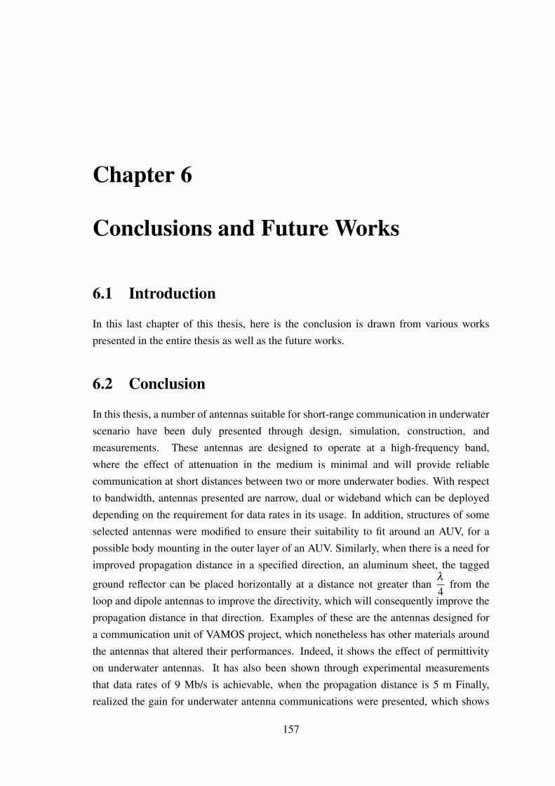
Chapter 6
Conclusions and Future Works
6.1 Introduction
In this last chapter of this thesis, here is the conclusion is drawn from various workspresented in the entire thesis as well as the future works.
6.2 Conclusion
In this thesis, a number of antennas suitable for short-range communication in underwaterscenario have been duly presented through design, simulation, construction, andmeasurements. These antennas are designed to operate at a high-frequency band,where the effect of attenuation in the medium is minimal and will provide reliablecommunication at short distances between two or more underwater bodies. With respectto bandwidth, antennas presented are narrow, dual or wideband which can be deployeddepending on the requirement for data rates in its usage. In addition, structures of someselected antennas were modified to ensure their suitability to fit around an AUV, for apossible body mounting in the outer layer of an AUV. Similarly, when there is a need forimproved propagation distance in a specified direction, an aluminum sheet, the tagged
ground reflector can be placed horizontally at a distance not greater thanλ
4from the
loop and dipole antennas to improve the directivity, which will consequently improve thepropagation distance in that direction. Examples of these are the antennas designed fora communication unit of VAMOS project, which nonetheless has other materials aroundthe antennas that altered their performances. Indeed, it shows the effect of permittivityon underwater antennas. It has also been shown through experimental measurementsthat data rates of 9 Mb/s is achievable, when the propagation distance is 5 m Finally,realized the gain for underwater antenna communications were presented, which shows
157
158 Conclusions and Future Works
that transmission and reception of signals in the underwater environment through radiowaves is possible at short propagation distance.
6.3 Future Work
For the furtherance of the work in underwater environments where submarines willhave diverse communications with satellite networks and terrestrial facilities, underwaterrobots will on one hand harvest data from sensor nodes and instantaneously transmit suchto locations above the water surface. Also, scuba divers will able to have real-time video,data and voice communications exchange with High Altitude Platform Stations (HAPS),all these will require a hybrid network of at least two of the underwater technologies.Thus, if radio waves communication is deployed as part of the hybrid network, thereforesome antennas are been proposed to be used in the network.
6.3.1 Miniaturized Underwater Antenna
A compact sized, self-similar antenna been proposed is fractal antennas. These can becategorized as deterministic or random types [13]. A particular type of deterministicfractal antenna been suggested for this application is known as snowflake fractal antenna.From an ordinary square loop (generator) to the 1st iteration, where outer lengths areabout 1.5 of the inner lengths, such that 8 outer lengths are equivalent to 12 inner lengths.Hence, 1st iteration has a total of 24 inner lengths if all the lengths are expressed in termsof inner lengths. A similar relationship exists between the lengths at the 4 edges and theinner lengths in the 4 wings of the 2nd iteration. Hence, generator, 1st iteration and 2nditeration as designed using FEKO software are presented in Fig. 6.1. It is worth notingthat 2nd iteration will occupy about 15.4% of the cross-sectional area of the generatorand details of the analyses of the lengths of these antennas are as presented in [164].Additionally, with the inclusion of ground reflector to this antenna, it can be made a highlydirectional in the medium, which will, therefore, improve the achievable propagationdistance.
6.3.2 Highly Directional Antenna
The double helical antenna presented in Fig. 5.35 of chapter 5 is a highly directionalantenna, which has exhibits high gain in the air. It is believed that the use of thistype of antenna in the underwater environment can enhance air-water cross-boundarycommunication. Indeed, the system will suffer from interface loss, which is dependent
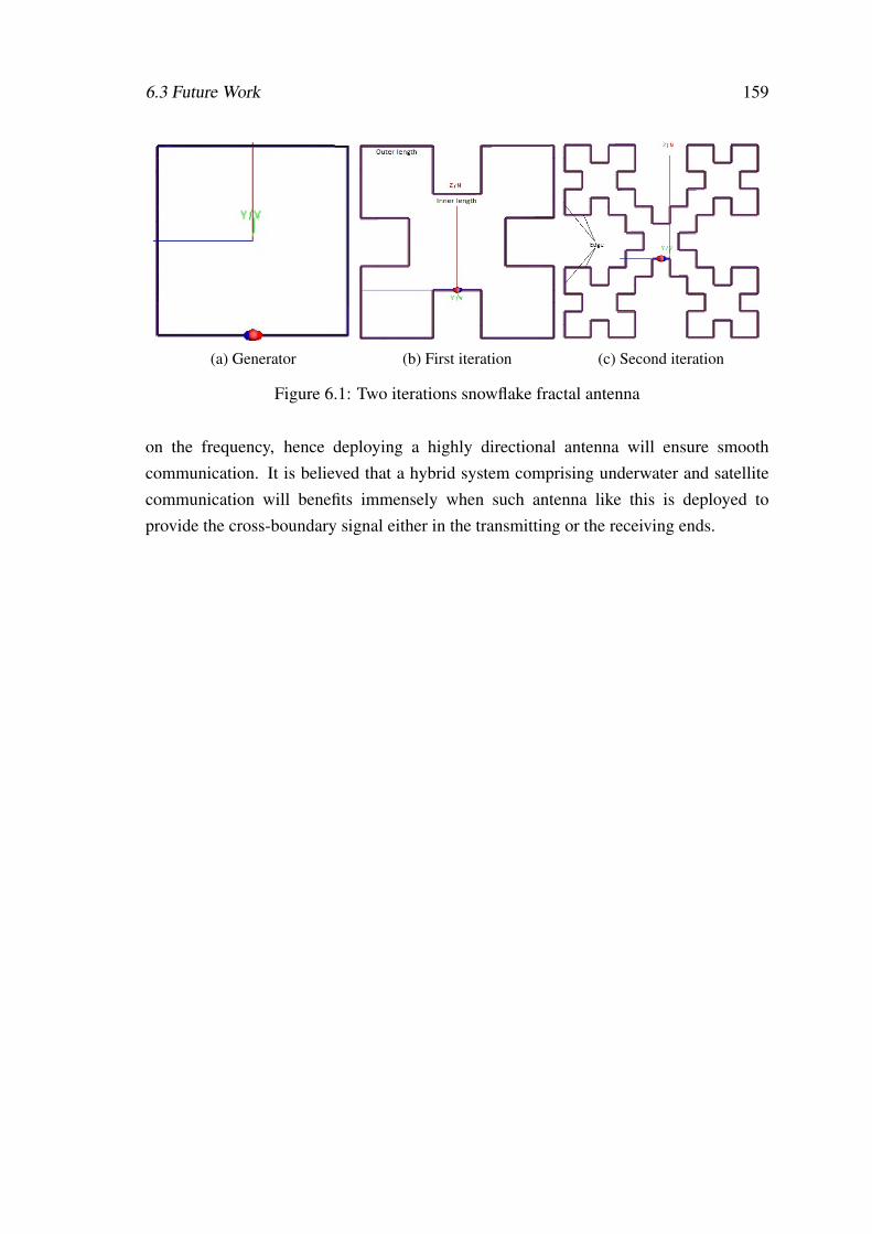
6.3 Future Work 159
(a) Generator (b) First iteration (c) Second iteration
Figure 6.1: Two iterations snowflake fractal antenna
on the frequency, hence deploying a highly directional antenna will ensure smoothcommunication. It is believed that a hybrid system comprising underwater and satellitecommunication will benefits immensely when such antenna like this is deployed toprovide the cross-boundary signal either in the transmitting or the receiving ends.

160 Conclusions and Future Works
Appendix A
BALUN
A.1 Definition
Balun is the codename for balance to unbalance. It is an electrical transformer or devicethat converts a balanced signal to unbalanced signal. It is also defined as a three-portpower splitter, which is similar to resistive power divider or Wilkinson. It has two output,which is equal in magnitude but has a 180 deg phase shift. In other words, it means thevoltages in the balance line are equal but with opposite signs. Balun is a reciprocal device,which implies that it can be used in the bidirectionally. Depending on the configuration,outputs of a balun may or may not have the same impedance as the input. For instance,a 1:1 balun is expected to have an input impedance the same with the outputs, whereas a4:1 balun sill have outputs impedances that are different from the input.
A.2 Balun in Underwater Antennas
In the designing of underwater antennas, a balun is used in two different ways. The first isto ensure matching of the input impedance to the desired 50 Ω source. But in some cases,due to the effect of the high permittivity of water, the input impedance is almost matched,a balun is still very important in the design to reduce the undesired radiation on the coaxialcable that could change some of the characteristics of the antennas by interfering with themeasured parameters. Thus, current baluns were used
161

References 162
References
[1] L. M. Pessoa, M. R. Pereira, H. M. Santos, and H. M. Salgado, “Simulation andexperimental evaluation of a resonant magnetic wireless power transfer system forseawater operation,” in OCEANS 2016 - Shanghai, April 2016, pp. 1–5.
[2] J. Lloret, S. Sendra, M. Ardid, and J. J. Rodrigues, “Underwater wireless sensorcommunications in the 2.4 ghz ism frequency band,” Sensors, vol. 12, no. 4, pp.4237–4264, 2012.
[3] S. Jiang and S. Georgakopoulos, “Electromagnetic wave propagation into freshwater,” Journal of Electromagnetic Analysis and Applications, vol. 3, no. 07, p.261, 2011.
[4] J. Goh, A. Shaw, and A. Al-Shamma’a, “Underwater wireless communicationsystem,” in Journal of Physics: Conference Series, vol. 178, no. 1. IOPPublishing, 2009, p. 012029.
[5] Z. Hao, G. Dawei, Z. Guoping, and T. A. Gulliver, “The impact of antennadesign and frequency on underwater wireless communications,” in Proceedingsof 2011 IEEE Pacific Rim Conference on Communications, Computers and SignalProcessing, Aug 2011, pp. 868–872.
[6] X. Che, I. Wells, G. Dickers, and P. Kear, “Tdma frame design for a prototypeunderwater rf communication network,” Ad Hoc Networks, vol. 10, no. 3, pp.317–327, 2012.
[7] S. Cerwin, Mobile and Maritime Antennas - The Super-J Maritime Antenna ,21st ed., D. Straw R, Ed. ARRL Amateur Radio, 2007.
[8] D. K. Cheng et al., Field and wave electromagnetics. Pearson Education India,1989.
[9] B. C. Hacker, “The machines of war: western military technology 1850–2000,”History and Technology, vol. 21, no. 3, pp. 255–300, 2005.
[10] R. E. Sheriff and Y. F. Hu, Mobile satellite communication networks. John Wiley& Sons, 2003.
[11] P. Sharma, “Evolution of mobile wireless communication networks-1g to 5g as wellas future prospective of next generation communication network,” International
163
References 164
Journal of Computer Science and Mobile Computing, vol. 2, no. 8, pp. 47–53,2013.
[12] “Ieee standard for definitions of terms for antennas,” IEEE Std 145-2013 (Revisionof IEEE Std 145-1993), pp. 1–50, March 2014.
[13] C. A. Balanis, “Antenna theory: analysis and design,” third edition, John wiley &sons, 2005.
[14] W. L. Stutzman and G. A. Thiele, Antenna theory and design. John Wiley & Sons,2012.
[15] T. A. Milligan, Modern antenna design. John Wiley & Sons, 2005.
[16] J. D. Kraus, Antennas. McGraw-Hill Education, 1988.
[17] Y. Huang and K. Boyle, Antennas: from theory to practice. John Wiley & Sons,2008.
[18] “Radio spectrum,” https://en.wikipedia.org/wiki/Radio_spectrum, accessed:2010-09-07.
[19] D. Roddy, Satellite Communications, (Professional Engineering). McGraw-HillProfessional: New York, 2006.
[20] H. Griffiths, L. Cohen, S. Watts, E. Mokole, C. Baker, M. Wicks, and S. Blunt,“Radar spectrum engineering and management: Technical and regulatory issues,”Proceedings of the IEEE, vol. 103, no. 1, pp. 85–102, 2015.
[21] R. Regulations, “International telecommunication union,” RadiocommunicationSector. ITU-R. Geneva, 2016.
[22] “QWH Series: Standard Gain Horn Antennas, howpublished =https://www.rfglobalnet.com/doc/qwh-series-standard-gain-horn-antennas-0002,”accessed: 2018-05-30.
[23] V. Midasala and P. Siddaiah, “Microstrip patch antenna array design to improvebetter gains,” Procedia Computer Science, vol. 85, pp. 401–409, 2016.
[24] E. Ebeleke, “’how nigcomsat will help achieve 30posted07-March-2018. [Online]. Available: https://www.vanguardngr.com/2018/03/nigcomsat-will-help-achieve-30-broadband-target/
[25] X. Che, I. Wells, G. Dickers, P. Kear, and X. Gong, “Re-evaluationof rf electromagnetic communication in underwater sensor networks,” IEEECommunications Magazine, vol. 48, no. 12, pp. 143–151, 2010.
[26] A. Gkikopouli, G. Nikolakopoulos, and S. Manesis, “A survey on underwaterwireless sensor networks and applications,” in Control & Automation (MED), 201220th Mediterranean Conference on. IEEE, 2012, pp. 1147–1154.
References 165
[27] C. Gussen, P. Diniz, M. Campos, W. A. Martins, F. M. Costa, and J. N. Gois, “Asurvey of underwater wireless communication technologies,” J. Commun. Inf. Sys.,vol. 31, no. 1, pp. 242–255, 2016.
[28] M. R. Frater, M. J. Ryan, and R. M. Dunbar, “Electromagnetic communicationswithin swarms of autonomous underwater vehicles,” in Proceedings of the 1st ACMinternational workshop on Underwater networks. ACM, 2006, pp. 64–70.
[29] Z. Xiao, H. Xiao, Y. Jingwei, and S. Xueli, “Study on doppler effects estimatein underwater acoustic communication,” The Journal of the Acoustical Society ofAmerica, vol. 133, no. 5, pp. 3463–3463, 2013.
[30] X. Guo, M. R. Frater, and M. J. Ryan, “A propagation-delay-tolerant collisionavoidance protocol for underwater acoustic sensor networks,” in OCEANS 2006- Asia Pacific, May 2006, pp. 1–6.
[31] Z. Zeng, S. Fu, H. Zhang, Y. Dong, and J. Cheng, “A survey of underwater opticalwireless communications,” IEEE Communications Surveys Tutorials, vol. 19, no. 1,pp. 204–238, Firstquarter 2017.
[32] L. Lanbo, Z. Shengli, and C. Jun-Hong, “Prospects and problems of wirelesscommunication for underwater sensor networks,” Wireless Communications andMobile Computing, vol. 8, no. 8, pp. 977–994, 2008.
[33] O. Aboderin, L. M. Pessoa, and H. M. Salgado, “Performance evaluation ofantennas for underwater applications,” in 2017 Wireless Days, March 2017, pp.194–197.
[34] A. Palmeiro, M. Martín, I. Crowther, and M. Rhodes, “Underwater radio frequencycommunications,” in OCEANS 2011 IEEE - Spain, June 2011, pp. 1–8.
[35] U. Chakraborty, T. Tewary, and R. Chatterjee, “Exploiting the loss-frequencyrelationship using rf communication in underwater communication networks,”in Computers and Devices for Communication, 2009. CODEC 2009. 4thInternational Conference on. IEEE, 2009, pp. 1–4.
[36] A. H. Taylor, “Short wave reception and transmission on ground wires(subterranean and submarine),” Proceedings of the Institute of Radio Engineers,vol. 7, no. 4, pp. 337–361, Aug 1919.
[37] W. H. Secor, “American greatest war invention,” Electrical Experimenter, vol. 6,no. 11, p. 5, 1919.
[38] R. Batcher, “Loop antenna for submarines,” Wireless age, vol. 7, p. 28, 1920.
[39] R. Llamas, Curved spiral antennas for underwater biological applications. TheUniversity of Iowa, 2015.
References 166
[40] K. C. Rao, P. M. Rao, and A. S. S. Rao, “Submarine based communicationover years: A review,” International Journal of Innovative Research in Science,Engineering and Technology, vol. 5, no. 12, pp. 20 983–20 995, 2016.
[41] V. R. Fisher, “The submerged receiving aerials,” The wireless Age, vol. 7, no. 6,p. 2, March 1920.
[42] G. O. Squier, “Transmission of high frequency waves over bare wires in water,”The wireless Age, vol. 7, no. 10, p. 2, July 1920.
[43] J. R. Wait, “The magnetic dipole over the horizontally stratified earth,” CanadianJournal of Physics, vol. 29, no. 6, pp. 577–592, 1951.
[44] J. R. Wait, “Current-Carrying Wire Loops in a Simple Inhomogeneous Region,”Journal of Applied Physics, vol. 23, no. 4, pp. 497–498, 1952.
[45] J. Wait, “Electromagnetic Fields of Current-Carrying Wires in a ConductingMedium,” Canadian Journal of Physics, vol. 30, pp. 512–523, Sep. 1952.
[46] J. R. Wait and L. L. Campbell, “The fields of an electric dipole in a semi-infiniteconducting medium,” Journal of Geophysical Research, vol. 58, no. 1, pp. 21–28,1953. [Online]. Available: <GotoISI>://WOS:A1953XX13300002
[47] J. R. Wait, “Insulated loop antenna immersed in a conducting medium,” Journal ofResearch of the National Bureau of Standards, vol. 59, no. 2, 1957.
[48] A. Banos Jr and J. P. Wesley, “The horizontal electric dipole in a conductinghalf-space,” Universi.ty of California, Tech. Rep., 1953.
[49] H. Wheeler, “Fundamental limitaions of a small vlf antenna for submarines,” IRETransactions on Antennas and Propagation, vol. 6, no. 1, pp. 123–125, January1958.
[50] W. Weeks and R. Fenwick, “Submerged antenna performance,” in 1958 IREInternational Convention Record, vol. 10, March 1962, pp. 108–135.
[51] R. W. Turner, “Submarine communication antenna systems,” Proceedings of theIRE, vol. 47, no. 5, pp. 735–739, May 1959.
[52] W. Anderson and R. Moore, “Frequency spectra of transient electromagnetic pulsesin a conducting medium,” IRE Transactions on Antennas and Propagation, vol. 8,no. 6, pp. 603–607, November 1960.
[53] R. Moore and W. Blair, “Dipole radiation in a conducting half-space,” J. Res. NBS,vol. 65, no. 6, pp. 547–563, 1961.
[54] S. Durrani, “Air-to-undersea communication with electric dipoles,” IRETransactions on Antennas and Propagation, vol. 10, no. 5, pp. 524–528, September1962.
References 167
[55] R. Hansen, “Radiation and reception with buried and submerged antennas,” IEEETransactions on Antennas and Propagation, vol. 11, no. 3, pp. 207–216, May 1963.
[56] R. King and K. Iizuka, “The complete electromagnetic field of a half-wave dipole ina dissipative medium,” IEEE Transactions on Antennas and Propagation, vol. 11,no. 3, pp. 275–285, May 1963.
[57] G. Hasserjian and A. Guy, “Low-frequency subsurface antennas,” IEEETransactions on Antennas and Propagation, vol. 11, no. 3, pp. 225–231, May 1963.
[58] R. Fenwick and W. Weeks, “Sumberged antenna characteristics,” IEEETransactions on Antennas and Propagation, vol. 11, no. 3, pp. 296–305, May 1963.
[59] R. Moore, “Effects of a surrounding conducting medium on antenna analysis,”IEEE Transactions on Antennas and Propagation, vol. 11, no. 3, pp. 216–225,May 1963.
[60] R. K. Moore, “Radio communication in the sea,” IEEE Spectrum, vol. 4, no. 11,pp. 42–51, Nov 1967.
[61] S. Durrani, “Air to undersea communication with magnetic dipoles,” IEEETransactions on Antennas and Propagation, vol. 12, no. 4, pp. 464–470, July 1964.
[62] R. King, B. Sandler, and T. Wu, “Cylindrical antennas immersed in arbitraryhomogeneous isotropic media,” Journal of Applied Physics, vol. 40, no. 13, pp.5049–5065, 1969.
[63] M. Siegel and R. King, “Radiation from linear antennas in a dissipative half-space,”IEEE Transactions on Antennas and Propagation, vol. 19, no. 4, pp. 477–485, Jul1971.
[64] C. Tsao, “Radiation resistance of antennas in lossy media,” IEEE Transactions onAntennas and Propagation, vol. 19, no. 3, pp. 443–444, May 1971.
[65] M. Burrows and C. Niessen, “Elf communication system design,” in Ocean 72 -IEEE International Conference on Engineering in the Ocean Environment, Sept1972, pp. 95–109.
[66] M. Siegel and R. King, “Electromagnetic propagation between antennassubmerged in the ocean,” IEEE Transactions on Antennas and Propagation,vol. 21, no. 4, pp. 507–513, Jul 1973.
[67] J. R. Wait, “Project sanguine,” Science, vol. 178, no. 4058, pp. 272–275, 1972.
[68] B. Keiser, “Early development of the project sanguine radiating system,” IEEETransactions on Communications, vol. 22, no. 4, pp. 364–371, April 1974.
[69] R. Moore, “A simplified estimate of sanguine performance,” in Ocean 72 - IEEEInternational Conference on Engineering in the Ocean Environment, Sept 1972,pp. 136–143.
References 168
[70] B. Kruger, “Sanguine system overview,” in Ocean 72 - IEEE InternationalConference on Engineering in the Ocean Environment, Sept 1972, pp. 91–94.
[71] C. Fessenden and D. Cheng, “Development of a trailing-wire e-field submarineantenna for extremely low frequency (elf) reception,” IEEE Transactions onCommunications, vol. 22, no. 4, pp. 428–437, Apr 1974.
[72] J. Merrill, “Some early historical aspects of project sanguine,” IEEE Transactionson Communications, vol. 22, no. 4, pp. 359–363, Apr 1974.
[73] J. Wait, “Historical background and introduction to the special issue on extremelylow frequency (elf) communications,” IEEE Transactions on Communications,vol. 22, no. 4, pp. 353–354, April 1974.
[74] S. L. Bernstein, M. L. Burrows, J. E. Evans, A. S. Griffiths, D. A. McNeill, C. W.Niessen, I. Richer, D. P. White, and D. K. Willim, “Long-range communications atextremely low frequencies,” Proceedings of the IEEE, vol. 62, no. 3, pp. 292–312,March 1974.
[75] S. Wolf, J. Davis, and M. Nisenoff, “Superconducting extremely low frequency(elf) magnetic field sensors for submarine communications,” IEEE Transactionson Communications, vol. 22, no. 4, pp. 549–554, Apr 1974.
[76] H. Momma and T. Tsuchiya, “Underwater communication by electric current,” inOCEANS ’76, Sept 1976, pp. 631–636.
[77] J. Davis, R. Dinger, and J. Goldstein, “Development of a superconducting elfreceiving antenna,” IEEE Transactions on Antennas and Propagation, vol. 25,no. 2, pp. 223–231, March 1977.
[78] J. Wait, “Propagation of elf electromagnetic waves and project sanguine/seafarer,”IEEE Journal of Oceanic Engineering, vol. 2, no. 2, pp. 161–172, Apr 1977.
[79] R. Decesari, “Buoyant module vhf antenna design for submerged systems/aircraftcommunications,” in OCEANS ’79, Sept 1979, pp. 366–372.
[80] A. Arutaki and J. Chiba, “Communication in a three-layered conducting mediawith a vertical magnetic dipole,” IEEE Transactions on Antennas and Propagation,vol. 28, no. 4, pp. 551–556, Jul 1980.
[81] M. Callaham, “Submarine communications,” IEEE Communications Magazine,vol. 19, no. 6, pp. 16–25, November 1981.
[82] D. L. Jones, “Sending signals to submarines,” New Scientist, vol. 106, no. 1463,pp. 37–41, 1985.
[83] L. B. VK5BR, “Underwater radio communication,” Originally published inAmateur Radio, 1987.
References 169
[84] R. M. Dunbar, “A surface-contour electromagnetic wave antenna for short-rangesubsea communications,” in Sixth International Conference on ElectronicEngineering in Oceanography, 1994., Jul 1994, pp. 117–123.
[85] B. Benhabiles, P. Lacour, M. Pellet, C. Pichot, and A. Papiernik, “A study of vlfantennas immersed in sea water: theoretical, numerical, and experimental results,”IEEE Antennas and Propagation Magazine, vol. 38, no. 5, pp. 19–29, Oct 1996.
[86] R. W. P. King, C. W. Harrison, and V. A. Houdzoumis, “Electromagnetic field inthe sea due to an omnidirectional vlf antenna,” Radio Science, vol. 32, no. 1, pp.103–112, Jan 1997.
[87] R. W. P. King, “Directional vlf antenna for communicating with submarines,”Radio Science, vol. 32, no. 1, pp. 113–125, Jan 1997.
[88] B. Aldridge, “Elf history: extremely low frequency communication,” PLRCPacificLife Research Center, Tech. Rep. PLRC-941005B, 2001.
[89] A. Monin, “Submarine floating antenna model for loran-c signal processing,” IEEETransactions on Aerospace and Electronic Systems, vol. 39, no. 4, pp. 1304–1315,Oct 2003.
[90] A. I. Al-Shamma’a, A. Shaw, and S. Saman, “Propagation of electromagneticwaves at mhz frequencies through seawater,” IEEE Transactions on Antennas andPropagation, vol. 52, no. 11, pp. 2843–2849, Nov 2004.
[91] A. Karlsson, “Physical limitations of antennas in a lossy medium,” IEEETransactions on Antennas and Propagation, vol. 52, no. 8, pp. 2027–2033, Aug2004.
[92] C. A. Altgelt, “The world’s largest "radio" station,” accessed from internet, 2005.
[93] R. Tamas, “Evaluation of the mutual coupling between shipborne antennas,” inEurope Oceans 2005, vol. 2, June 2005, pp. 1343–1346 Vol. 2.
[94] A. Shaw, A. i. Al-Shamma’a, S. R. Wylie, and D. Toal, “Experimentalinvestigations of electromagnetic wave propagation in seawater,” in 2006 EuropeanMicrowave Conference, Sept 2006, pp. 572–575.
[95] F. Plonski and C. M. Gyenes, “Efficient hf submarine antennas,” in 2008 IEEEAntennas and Propagation Society International Symposium, July 2008, pp. 1–4.
[96] C. Liu, L.-G. Zheng, and Y.-P. Li, “Study of elf electromagnetic fields froma submerged horizontal electric dipole positioned in a sea of finite depth,”in Microwave, Antenna, Propagation and EMC Technologies for WirelessCommunications, 2009 3rd IEEE International Symposium on. IEEE, 2009, pp.152–157.

References 170
[97] Y. Cai and R. Ding, “Application of superconductor in elf communication,” in2009 International Conference on Applied Superconductivity and ElectromagneticDevices, Sept 2009, pp. 77–80.
[98] B. Austin, “Signalling to submarines at extremely low frequencies,” RadioBygones, no. 118, pp. 10–17, 2009.
[99] A. Garcia Miquel, “Uwb antenna design for underwater communications,” Ph.D.dissertation, Universitat Politecnica de Catalunya, 2009.
[100] R. M. Dunbar, M. R. Frater, M. J. Ryan, and G. N. Milford, “Underseaelectromagnetic networking,” in 2011 Military Communications and InformationSystems Conference, Nov 2011, pp. 1–9.
[101] G. Thompson, H. Widmer, K. Rice, R. Ball, and J. Sweeney, “Buoyant cableantenna technology for enhancing submarine communications atspeed and depth,”Johns Hopkins APL technical digest, vol. 20, no. 3, pp. 285–296, 1999.
[102] A. M. Karim, S. J. Stafford, and R. Benjamin Baker, “Global positioning systemover fiber for buoyant cable antennas,” Johns Hopkins APL Technical Digest,vol. 30, no. 4, pp. 309–320, 2012.
[103] B. Kelley and K. Naishadham, “High data rate undersea broadband radio-frequencycommunications,” in 2014 IEEE Antennas and Propagation Society InternationalSymposium (APSURSI), July 2014, pp. 695–696.
[104] M. Manteghi and A. A. Y. Ibraheem, “On the study of the near-fields of electricand magnetic small antennas in lossy media,” IEEE Transactions on Antennas andPropagation, vol. 62, no. 12, pp. 6491–6495, Dec 2014.
[105] H. Wang, K. Zheng, K. Yang, and Y. Ma, “Electromagnetic field in air producedby a horizontal magnetic dipole immersed in sea: Theoretical analysis andexperimental results,” IEEE Transactions on Antennas and Propagation, vol. 62,no. 9, pp. 4647–4655, Sept 2014.
[106] M. Manteghi, “An electrically small antenna for underwater applications,” in 2016IEEE International Symposium on Antennas and Propagation (APSURSI), June2016, pp. 1745–1746.
[107] A. Massaccesi and P. Pirinoli, “Analysis of antennas for underwater applications,”in 2017 11th European Conference on Antennas and Propagation (EUCAP), March2017, pp. 1907–1910.
[108] G. S. Saran and G. Held, “Field strength mesurements in fresh water,” Journal ofResearch of the National Bureau of Standards D, vol. 52, pp. 435–437, 1960.
[109] M. Siegel and R. W. King, “Electromagnetic fields in a dissipative half-space: Anumerical approach,” Journal of Applied Physics, vol. 41, no. 6, pp. 2415–2423,1970.
References 171
[110] L. Shen, R. W. King, and R. Sorbello, “Measured field of a directional antennasubmerged in a lake,” IEEE Transactions on Antennas and Propagation, vol. 24,no. 6, pp. 891–894, Nov 1976.
[111] L. C. Shen, K. M. Lee, and R. W. P. King, “Coupled horizontal-wire antennas overa conducting or dielectric half space,” Radio Science, vol. 12, no. 5, pp. 687–698,Sept 1977.
[112] H. M. Hafez, W. J. Chudobiak, and J. S. Wight, “The attenuation rate in fresh waterat vhf frequencies,” IEEE Transactions on Instrumentation and Measurement,vol. 28, no. 1, pp. 71–74, March 1979.
[113] L. N. An and G. S. Smith, “The horizontal circular loop antenna near a planarinterface,” Radio Science, vol. 17, no. 03, pp. 483–502, May 1982.
[114] G. S. Smith and L. N. An, “Loop antennas for directive transmission into a materialhalf space,” Radio Science, vol. 18, no. 05, pp. 664–674, Sept 1983.
[115] G. Smith, “Directive properties of antennas for transmission into a materialhalf-space,” IEEE Transactions on Antennas and Propagation, vol. 32, no. 3, pp.232–246, March 1984.
[116] F. Travade, P. Bomassi, J. Bach, C. Brugel, P. Stein-bach, J. Luquet, andG. Pustelnik, “Use of radiotracking in france for recent studies concerning the edffishways program,” Hydroécologie Appliquée, vol. 1, pp. 33–51, 1989.
[117] J. W. Beeman, C. Grant, and P. V. Haner, “Comparison of three underwaterantennas for use in radiotelemetry,” North American Journal of FisheriesManagement, vol. 24, no. 1, pp. 275–281, 2004.
[118] R. Zhou, H. Zhang, and H. Xin, “A compact water based dielectric resonatorantenna,” in 2009 IEEE Antennas and Propagation Society InternationalSymposium, June 2009, pp. 1–4.
[119] C. Conessa and A. Joisel, “Active wideband antenna for underwater tomography(1 ghz),” Electronics Letters, vol. 45, no. 4, pp. 193–194, February 2009.
[120] K. P. Hunt, J. J. Niemeier, and A. Kruger, “Short paper: Antennas for mussel-basedunderwater biological sensor networks in rivers,” WUWNET, ACM, 2010.
[121] H. F. G. Mendez, C. Gac, F. L. Pennec, and C. Person, “High performanceunderwater uhf radio antenna development,” in OCEANS 2011 IEEE - Spain, June2011, pp. 1–5.
[122] A. A. Abdou, A. Shaw, A. Mason, A. Al-Shamma’a, J. Cullen, and S. Wylie,“Electromagnetic (em) wave propagation for the development of an underwaterwireless sensor network (wsn),” in 2011 IEEE SENSORS Proceedings, Oct 2011,pp. 1571–1574.
References 172
[123] S. Kumar, “Design and comparison of modified circular bow-tie antenna for underwater radio communication by optimized parameters,” International Journal ofInnovative Research in Technology & Science (IJIRTS), 2012.
[124] A. Abdou, A. Shaw, A. Mason, A. Al-Shamma’a, J. Cullen, S. Wylie, andM. Diallo, “A matched bow-tie antenna at 433mhz for use in underwater wirelesssensor networks,” in Journal of Physics: Conference Series, vol. 450, no. 1. IOPPublishing, 2013, pp. 1–7.
[125] S. Sendra, J. Lloret, J. J. P. C. Rodrigues, and J. M. Aguiar, “Underwater wirelesscommunications in freshwater at 2.4 ghz,” IEEE Communications Letters, vol. 17,no. 9, pp. 1794–1797, September 2013.
[126] E. A. Karagianni, “Electromagnetic waves under sea: bow-tie antennas designfor wi-fi underwater communications,” Progress In Electromagnetics Research,vol. 41, pp. 189–198, 2015.
[127] H. Yoshida, N. Iwakiri, T. Fukuda, M. Deguchi, and S. Onogi, “Measurementsof underwater electromagnetic wave propagation,” in 2015 IEEE UnderwaterTechnology (UT), Feb 2015, pp. 1–5.
[128] R. A. Llamas, J. J. Niemeier, and A. Kruger, “Curved spiral antennas for freshwaterapplications,” in 2015 IEEE Radio and Wireless Symposium (RWS), Jan 2015, pp.53–55.
[129] A. Massaccesi and P. Pirinoli, “Preliminary results on cylindrical antennas forunderwater communication,” in 2016 IEEE International Symposium on Antennasand Propagation (APSURSI), June 2016, pp. 1895–1896.
[130] D. M. Pozar, Microwave Engineering. John Wiley & Sons, 2011.
[131] M. R. S. Pereira, Inverse Scattering Techniques for the Synthesis of MicrowaveStructures. Universidade do Porto, 2014.
[132] R. E. Collin, Foundations for Microwave Engineering. John Wiley & Sons, 2007.
[133] K. S. Cole and R. H. Cole, “Dispersion and absorption in dielectrics i. alternatingcurrent characteristics,” The Journal of chemical physics, vol. 9, no. 4, pp.341–351, 1941.
[134] F. Franks, The physics and physical chemistry of water. Springer Science &Business Media, 2012, vol. 1.
[135] R. Somaraju and J. Trumpf, “Frequency, temperature and salinity variation ofthe permittivity of seawater,” IEEE Transactions on Antennas and Propagation,vol. 54, no. 11, pp. 3441–3448, Nov 2006.
[136] F. T. Ulaby, U. Ravaioli, and E. Michielssen, Fundamentals of appliedelectromagnetics. Prentice Hall, 2014.
References 173
[137] L. Klein and C. Swift, “An improved model for the dielectric constant of sea waterat microwave frequencies,” IEEE Journal of Oceanic Engineering, vol. 2, no. 1,pp. 104–111, 1977.
[138] S. I. Inácio, M. R. Pereira, H. M. Santos, L. M. Pessoa, F. B. Teixeira, M. J.Lopes, O. Aboderin, and H. M. Salgado, “Antenna design for underwater radiocommunications,” in OCEANS 2016 - Shanghai, April 2016, pp. 1–6.
[139] L. M. Pessoa, M. R. Pereira, O. Aboderin, H. M. Salgado, and S. I. Inácio,“Antenna for underwater radio communications,” patentep 3 291 364A1.
[140] P. A. Mendez and R. James, “A comparative study of underwater wireless opticalcommunication for three different communication links,” Journal of Electronicsand Communication Engineering, vol. 10, no. 3, pp. 40–48, 2015.
[141] F. Teixeira, P. Freitas, L. Pessoa, R. Campos, and M. Ricardo, “Evaluation ofieee 802.11 underwater networks operating at 700 mhz, 2.4 ghz and 5 ghz,” inProceedings of the International Conference on Underwater Networks & Systems.ACM, 2014, p. 11.
[142] A. Netchaev, J. Klein, C. Thurmer, B. Carver, and J. Evans, “Medium rangeunderwater communication development system,” in 2016 IEEE SENSORS, Oct2016, pp. 1–3.
[143] C. A. Balanis, “Antenna theory: a review,” Proceedings of the IEEE, vol. 80, no. 1,pp. 7–23, Jan 1992.
[144] Y. Rahmat-Samii, L. I. Williams, and R. G. Yaccarino, “The ucla bi-polarplanar-near-field antenna-measurement and diagnostics range,” IEEE Antennasand Propagation Magazine, vol. 37, no. 6, pp. 16–35, Dec 1995.
[145] A. H. F. S. Simulator, “Version 10.0,” Ansoft Corporation, 2005.
[146] A. Boyer, “Getting started with feko software,” National Institute of AppliedSciences Toulouse, 2008.
[147] S. I. Inácio, M. R. Pereira, H. M. Santos, L. M. Pessoa, F. B. Teixeira,M. J. Lopes, O. Aboderin, and H. M. Salgado, “Dipole antenna for underwaterradio communications,” in 2016 IEEE Third Underwater Communications andNetworking Conference (UComms), Aug 2016, pp. 1–5.
[148] M. Rhodes, “Underwater electromagnetic propagation: re-evaluating wirelesscapabilities,” Hydro International, vol. 10, no. 10, pp. 28–31, 2006.
[149] V. Bhavsar, N. Blas, H. Nguyen, and A. Balandin, “Measurement of antennaradiation patterns laboratory manual,” EE117 Laboratory Manual, UC-Riverside,Retrieved on April, vol. 20, no. 2010, pp. 1–42, 2000.
[150] H. Beggerow, “Zeppelin antenna,” 1909.

[151] J. S. Huggins, “Improving the super j-pole antenna,” 2012.
[152] A. R. Djordjevic, A. G. Zajic, M. M. Ilic, and G. L. Stüber, “Optimization of helicalantennas,” IEEE Antennas and Propagation Magazine, vol. 48, no. 6, pp. 107–115,2006.
[153] N. A. Cruz and A. C. Matos, “The mares auv, a modular autonomous robot forenvironment sampling,” in OCEANS 2008, Sept 2008, pp. 1–6.
[154] N. A. Cruz, A. C. Matos, R. M. Almeida, B. M. Ferreira, and N. Abreu, “Trimares-ahybrid auv/rov for dam inspection,” in OCEANS 2011. IEEE, 2011, pp. 1–7.
[155] A. Matos, N. Cruz, and F. L. Pereira, “Post mission trajectory smoothing for theisurus auv,” in Oceans 2003. Celebrating the Past ... Teaming Toward the Future(IEEE Cat. No.03CH37492), vol. 2, Sept 2003, pp. 683–687 Vol.2.
[156] A. Ayorinde, S. Adekola, A. I. Mowete, and W. Island, “Performancecharacteristics of loop antennas above a ground plane of finite extent,” in PIERSProceedings, 2013, pp. 769–744.
[157] D. Jefferies, “Experiments on loops above ground,” antenneX Online, no. 106, p. 8,2006.
[158] J. Iwashige, “Analysis of loop antenna with circular reflector and its properties,”Electronics and Communications in Japan (Part I: Communications), vol. 63,no. 11, pp. 44–50, 1980.
[159] O. Aboderin, S. I. Inacio, H. M. Santos, M. R. Pereira, L. M. Pessoa,and H. M. Salgado, “Analysis of j-pole antenna configurations for underwatercommunications,” in OCEANS 2016 MTS/IEEE Monterey, Sept 2016, pp. 1–5.
[160] J. Almeida, A. Ferreira, B. Matias, A. Dias, A. Martins, F. Silva, J. Oliveira,P. Sousa, M. Moreira, T. Miranda et al., “Air and underwater survey of waterenclosed spaces for vamos! project,” in OCEANS 2016 MTS/IEEE Monterey.IEEE, 2016, pp. 1–5.
[161] C. Sword, B. Bodo, S. Kapusniak, F. Bosman, J. Rainbird, and E. Silva, “¡ vamos!(viable alternative mine operating system) - a ’horizon 2020’ project,” in EGUGeneral Assembly Conference Abstracts, vol. 19, 2017, p. 348.
[162] M. Bleier, A. Dias, A. Ferreira, J. Pidgeon, J. Almeida, E. Silva, K. Schilling,and A. Nüchter, “Real-time 3d Mine Modelling in the ¡vamos! Project,” pp. 1–12,2017.
[163] J. R. Pereira, “Projeto de up-down converter e antena para comunicações wi-fisub-aquáticas,” 2018.
[164] F. Hughes, “Fractal type antennas,” http://www.vk6fh.com/vk6fh/fractal.htm, 2013,accessed: 2018-07-15.