an initial value problem arising in mechanics
TRANSCRIPT

arX
iv:1
208.
4860
v2 [
mat
h-ph
] 1
7 D
ec 2
012
On a initial value problem arising in mechanics
Teodor M. Atanackovic∗, Stevan Pilipovic† and Dusan Zorica‡
December 23, 2013
Abstract
We study initial value problem for a system consisting of an integer order and distributed-
order fractional differential equation describing forced oscillations of a body attached to a
free end of a light viscoelastic rod. Explicit form of a solution for a class of linear viscoelastic
solids is given in terms of a convolution integral. Restrictions on storage and loss moduli
following from the Second Law of Thermodynamics play the crucial role in establishing the
form of the solution. Some previous results are shown to be special cases of the present
analysis.
Keywords: distributed-order fractional differential equation, fractional viscoelastic mate-
rial, forced oscillations of a body
1 Introduction
We study the initial value problem given by
∫ 1
0
φσ (γ) 0Dγt σ (t) dγ =
∫ 1
0
φε (γ) 0Dγt ε (t) dγ, t > 0, (1)
−σ (t) + F (t) =d2
dt2ε (t) , t > 0, (2)
σ (0) = 0, ε (0) = 0,d
dtε (0) = 0. (3)
In (1) - (3) we use σ to denote stress, ε denotes strain and F denotes the force acting at the freeend of a rod. The left Riemann-Liouville fractional derivative of order γ ∈ (0, 1) is defined by
0Dγt y (t) :=
d
dt
(
t−γ
Γ (1− γ)∗ y (t)
)
, t > 0,
see [7]. The Euler gamma function is denoted by Γ and ∗ denotes the convolution: (f ∗ g) (t) :=∫ t
0f (τ ) g (t− τ ) dτ , t ∈ R, if f, g ∈ L1
loc (R) and supp f, g ⊂ [0,∞). The displacement of anarbitrary point of a rod that is at the initial moment at the position x is
u (x, t) = xε (t) , t > 0, x ∈ [0, 1] ,
∗Department of Mechanics, Faculty of Technical Sciences, University of Novi Sad, Trg D. Obradovica 6, 21000
Novi Sad, Serbia, [email protected]†Department of Mathematics, Faculty of Natural Sciences and Mathematics, University of Novi Sad, Trg D.
Obradovica 4, 21000 Novi Sad, Serbia, [email protected]‡Mathematical Institute, Serbian Academy of Arts and Sciences, Kneza Mihaila 36, 11000 Beograd, Serbia,
dusan [email protected]
1

see [1].Equation (1) represents a constitutive equation of a viscoelastic rod, (2) is equation of motion
of a body attached to a free end of a rod and (3) represent the initial conditions. For the studyof waves in viscoelastic materials of fractional type see [6].
The derivation of the system (1) - (3) is given in [1], where the special case of (1) is consideredwhen the constitutive functions φσ and φε have the form
φσ (γ) = aγ and φε (γ) = c δ (γ) + bγ , 0 < a ≤ b, c > 0,
where δ is the Dirac delta distribution. In the present work we allow constitutive functions(or distributions) φσ and φε to be arbitrary satisfying Condition 1 and Assumption 4. To bephysically admissible (1) must satisfy two conditions: one being mathematical, the other beingphysical. The first condition that is essential on the level of generality treated in the workrequires that to real forcing (σ is a real-valued function of real variable) there corresponds a realresponse ε (ε is a real-valued function of real variable). This mathematical condition, that webelieve is new, is precisely formulated as (i) of Condition 1. The second condition is physicaland requires that in any closed deformation cycle there is a dissipation of energy. This is theformulation of the Second Law of Thermodynamics for isothermal processes. This condition isstated in its equivalent form as (ii) of Condition 1.
2 Analysis of the problem
In the following we use the Laplace transform method. The Laplace transform is defined by
f (s) = L [f (t)] (s) :=
∫ ∞
0
f (t) e−stdt, Re s > k,
where f ∈ L1loc (R) , f ≡ 0 in (−∞, 0] and |f (t)| ≤ cekt, t > 0, for some k > 0. We denote by
S ′ (R) the space of tempered distributions on R, while S ′+ is its subspace consisting of tempered
distributions with support [0,∞) . We refer to [8] for the properties of this space as well as forthe Laplace transform within it. We also use C
(
[0, 1] ,S ′+
)
to denote the space of continuousfunctions on [0, 1] with the values in S ′
+.
Applying formally the Laplace transform to (1) - (3) we get
σ (s)
∫ 1
0
φσ (γ) sγdγ = ε (s)
∫ 1
0
φε (γ) sγdγ, s ∈ D, (4)
σ (s) + s2ε (s) = F (s) , s ∈ D. (5)
By (4) we have
σ (x, s) =1
M2 (s)ε (x, s) , s ∈ D, (6)
where
M (s) :=
√
√
√
√
∫ 1
0φσ (γ) s
γdγ∫ 1
0 φε (γ) sγdγ
, s ∈ D ⊂ C. (7)
Note that for s = iω we obtain the complex modulus (see [4])
E (ω) = E′ (ω) + iE′′ (ω) :=1
M2 (iω)=
∫ 1
0φε (γ) (iω)
γ dγ∫ 1
0 φσ (γ) (iω)γdγ
, ω ∈ (0,∞) . (8)
2

Functions E′ and E′′ are real-valued and represent the storage and loss modulus, respectively.By (5) and (6) we have
ε (s) = F (s) P (s) , σ (s) = F (s) Q (s) , s ∈ D, (9)
where
P (s) :=M2 (s)
1 + (sM (s))2 , Q (s) :=
1
1 + (sM (s))2 , s ∈ D, (10)
and M is given by (7).Formally, by inverting the Laplace transform in (9), we obtain
ε (t) = F (t) ∗ P (t) , σ (t) = F (t) ∗Q (t) , t > 0. (11)
We discuss the restrictions that φσ and φε must satisfy. The first restriction follows from thefact that P and Q must be real-valued functions, so that strain ε and stress σ, given by (11), arereal. The second condition imposes the Second Law of Thermodynamics, which requires that (inisothermal case) the dissipation work must be positive. Mathematically, these conditions readas follows.
Condition 1
(i) There exists x0 ∈ R such that
M (x) =
√
√
√
√
∫ 1
0φσ (γ)x
γdγ∫ 1
0 φε (γ)xγdγ
∈ R, for all x > x0.
(ii) For all ω ∈ (0,∞) we haveE′ (ω) ≥ 0, E′′ (ω) ≥ 0,
where E′ and E′′ are storage and loss moduli, respectively, given by (8), see [4].
The motivation for (i) of Condition 1 follows from the following theorem of Doetsch.
Theorem 2 ([5, p. 293, Satz 2]) Let f(s) = L[F ](s), Re s > x0 ∈ R, be real-valued on thereal half-line s ∈ (x0,∞) . Then function F is real-valued almost everywhere.
Alternatively, if f is real-valued at a sequence of equidistant points on the real axis, thenfunction F is real-valued almost everywhere.
If φσ and φε are such that (i) of Condition 1 is satisfied, Theorem 2 ensures that inversions of(9) with (10), given by (11), are real. As it is well-known, [4], (ii) of Condition 1 guarantees thatthe Second Law of Thermodynamics for the isothermal process is satisfied. We shall see fromProposition 5 below that Condition 1 along with an additional assumption on the asymptotics ofM (Assumption 4 below) guarantees that the poles of the solution kernel in the Laplace domain(10) belong to the left complex half-plane. In this case the amplitude of the solution decreaseswith the time; this is a characteristic behavior for a dissipative process.
Remark 3
3

(i) Condition 1 is satisfied for the fractional Zener model
(1 + a 0Dαt )σ (t) = (1 + b 0D
αt ) ε (t) (12)
and for the distributed-order model
∫ 1
0
aγ 0Dγt σ (t) dγ =
∫ 1
0
bγ 0Dγt ε (t) dγ, (13)
In those case the function M takes the following forms
M (s) =
√
1 + asα
1 + bsα, s ∈ C\ (−∞, 0] , 0 < a ≤ b, α ∈ (0, 1) , (14)
M (s) =
√
ln (bs)
ln (as)
as− 1
bs− 1, s ∈ C\ (−∞, 0] , 0 < a ≤ b, (15)
respectively. Putting s = x ∈ R in the previous expressions we see that (i) of Condition 1is satisfied with x0 = 0, while 0 < a ≤ b ensures that (ii) of Condition 1 is satisfied, see[2, 4].
(ii) In general, stress σ as a function of a real-valued strain ε may not be real-valued. In [3] wehave such a situation, because (i) of Condition 1 is not satisfied. This shows the importanceof (i) of Condition 1.
3 Inversion of the Laplace transforms
In order to obtain ε and σ, by (9) we have to determine functions P and Q, i.e., to invert theLaplace transform in (10). We need an additional assumption on the function M, given by (7).
Assumption 4 Let M be of the form
M (s) = r (s) + ih (s) , as |s| → ∞,
and suppose that
lim|s|→∞
r (s) = c∞ > 0, lim|s|→∞
h (s) = 0, lim|s|→0
M (s) = c0,
for some constants c∞, c0 > 0.
Assumption 4 is motivated by the fractional Zener (12) and distributed-order model (13).We note that both of these models describe the viscoelastic solid-like body. For the both modelsmentioned above we have c∞ =
√
ab, and c0 = 1.
Proposition 5 Let M satisfy Condition 1 with x0 = 0 and Assumption 4. Let
f (s) := 1 + (sM (s))2, s ∈ C. (16)
Then f has two different zeros: s0 and its complex conjugate s0, located in the left complexhalf-plane (Re s < 0). The multiplicity of each zero is one.
4
Re s
Im s
gR3 g
R2
gR1
gL3
gL2
gL1
gR4
gL4
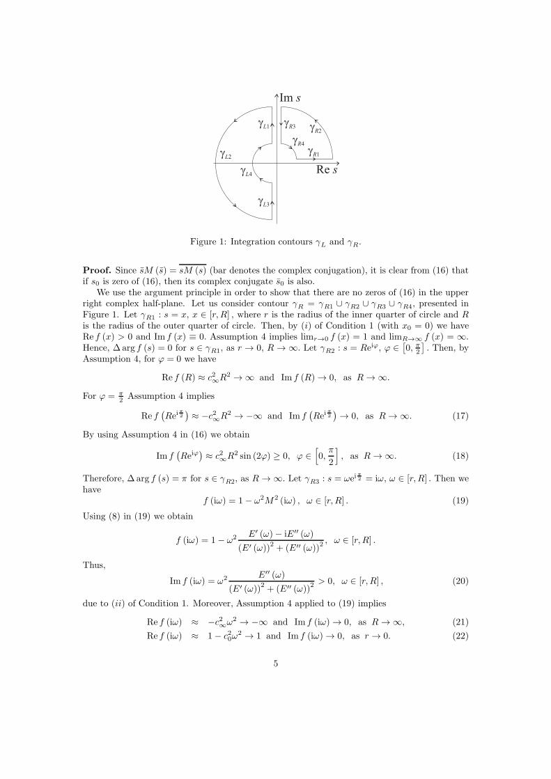
Figure 1: Integration contours γL and γR.
Proof. Since sM (s) = sM (s) (bar denotes the complex conjugation), it is clear from (16) thatif s0 is zero of (16), then its complex conjugate s0 is also.
We use the argument principle in order to show that there are no zeros of (16) in the upperright complex half-plane. Let us consider contour γR = γR1 ∪ γR2 ∪ γR3 ∪ γR4, presented inFigure 1. Let γR1 : s = x, x ∈ [r, R] , where r is the radius of the inner quarter of circle and R
is the radius of the outer quarter of circle. Then, by (i) of Condition 1 (with x0 = 0) we haveRe f (x) > 0 and Im f (x) ≡ 0. Assumption 4 implies limr→0 f (x) = 1 and limR→∞ f (x) = ∞.
Hence, ∆ arg f (s) = 0 for s ∈ γR1, as r → 0, R → ∞. Let γR2 : s = Reiϕ, ϕ ∈[
0, π2
]
. Then, byAssumption 4, for ϕ = 0 we have
Re f (R) ≈ c2∞R2 → ∞ and Im f (R) → 0, as R → ∞.
For ϕ = π2 Assumption 4 implies
Re f(
Reiπ2
)
≈ −c2∞R2 → −∞ and Im f(
Reiπ2
)
→ 0, as R → ∞. (17)
By using Assumption 4 in (16) we obtain
Im f(
Reiϕ)
≈ c2∞R2 sin (2ϕ) ≥ 0, ϕ ∈[
0,π
2
]
, as R → ∞. (18)
Therefore, ∆ arg f (s) = π for s ∈ γR2, as R → ∞. Let γR3 : s = ωeiπ2 = iω, ω ∈ [r, R] . Then we
havef (iω) = 1− ω2M2 (iω) , ω ∈ [r, R] . (19)
Using (8) in (19) we obtain
f (iω) = 1− ω2 E′ (ω)− iE′′ (ω)
(E′ (ω))2 + (E′′ (ω))2, ω ∈ [r, R] .
Thus,
Im f (iω) = ω2 E′′ (ω)
(E′ (ω))2+ (E′′ (ω))
2 > 0, ω ∈ [r, R] , (20)
due to (ii) of Condition 1. Moreover, Assumption 4 applied to (19) implies
Re f (iω) ≈ −c2∞ω2 → −∞ and Im f (iω) → 0, as R → ∞, (21)
Re f (iω) ≈ 1− c20ω2 → 1 and Im f (iω) → 0, as r → 0. (22)
5

We conclude that ∆arg f (s) = −π for s ∈ γR3, as r → 0, R → ∞. Let γR4 : s = reiϕ, ϕ ∈[
0, π2]
.
Assumption 4, for ϕ = 0 and ϕ = π2 implies
Re f (r) ≈ 1 + c20r2 → 1 and Im f (r) → 0, as r → 0,
Re f(
reiπ2
)
≈ 1− c20r2 → 1 and Im f
(
reiπ2
)
→ 0, as r → 0, (23)
as well as
Re f(
reiϕ)
≈ 1 + c20r2 cos (2ϕ) → 1 and Im f
(
reiϕ)
≈ c20r2 sin (2ϕ) → 0, (24)
for ϕ ∈[
0, π2]
, as r → 0. We see that ∆arg f (s) = 0 for s ∈ γR4, as r → 0. Thus, we concludethat
∆arg f (s) = 0 for s ∈ γR, as r → 0, R → ∞.
By the argument principle and that fact that the zeros are complex conjugated we conclude thatf has no zeros in the right complex half-plane.
We shall again use the argument principle and show that there are two zeros of (16) in theleft complex half-plane. Let us consider contour γL = γL1 ∪γL2 ∪γL3 ∪γL4, presented in Figure1. Let γL1 : s = ωei
π2 = iω, ω ∈ [r, R] . Then (20), (21) and (22) hold. Thus, ∆ arg f (s) = π for
s ∈ γL1, as r → 0, R → ∞. Let γL2 : s = Reiϕ, ϕ ∈[
π2 ,
3π2
]
. Then, for ϕ = π2 we have that (17)
holds. For ϕ = π Assumption 4 implies
Re f(
Reiπ)
≈ c2∞R2 → ∞ and Im f(
Reiπ)
→ 0, as R → ∞,
while for ϕ = 3π2 it implies
Re f(
Rei3π2
)
≈ −c2∞R2 → −∞ and Im f(
Rei3π2
)
→ 0, as R → ∞.
By (18), we have
Im f(
Reiϕ)
≈ c2∞R2 sin (2ϕ) ≤ 0, ϕ ∈[π
2, π)
, as R → ∞,
Im f(
Reiϕ)
≈ c2∞R2 sin (2ϕ) ≥ 0, ϕ ∈
(
π,3π
2
]
, as R → ∞.
We conclude that ∆arg f (s) = 2π for s ∈ γL2, as R → ∞. Let γL3 : s = ωei3π2 = −iω, ω ∈ [r, R] .
By (16) we havef (−iω) = 1− ω2M2 (iω), ω ∈ [r, R] , (25)
since M (s) = M (s). Using (8) in (25) we obtain
f (−iω) = 1− ω2 E′ (ω) + iE′′ (ω)
(E′ (ω))2 + (E′′ (ω))2, ω ∈ [r, R] .
Thus,
Im f (−iω) = −ω2 E′′ (ω)
(E′ (ω))2 + (E′′ (ω))2< 0, ω ∈ [r, R] ,
due to (ii) of Condition 1. Note that Assumption 4 applied to (25) implies
Re f (−iω) ≈ −c2∞ω2 → −∞ and Im f (iω) → 0, as R → ∞,
Re f (−iω) ≈ 1− c20ω2 → 1 and Im f (iω) → 0, as r → 0.
6

We conclude that ∆arg f (s) = π for s ∈ γL3, as r → 0, R → ∞. Let γL4 : s = reiϕ, ϕ ∈[
π2 ,
3π2
]
.
Then, for ϕ = π2 we have that (23) holds. For ϕ = 3π
2 Assumption 4 implies
Re f(
rei3π2
)
≈ 1− c20r2 → 1 and Im f
(
rei3π2
)
→ 0, as r → 0.
We have that also (24) holds for ϕ ∈[
π2 ,
3π2
]
, as r → 0, so that ∆arg f (s) = 0 for s ∈ γL4, asr → 0. Thus, the conclusion is that
∆arg f (s) = 4π for s ∈ γL, as r → 0, R → ∞.
This implies that f has two zeros in the left complex half-plane.The following theorem is related to the existence of solutions to system (1) - (3).
Theorem 6 Let M satisfy Condition 1 with x0 = 0 and Assumption 4. Let F ∈ S ′+.
(i) The displacement u as a part of the solution to (1) - (3), is given by
u (x, t) = xε (t) , where ε (t) = F (t) ∗ P (t) , x ∈ [0, 1] , t > 0, (26)
and
P (t) =1
π
∫ ∞
0
Im
(
M2(
qe−iπ)
1 + (qM (qe−iπ))2
)
e−qtdq + 2Re(
Res(
P (s) est, s0
))
, t > 0,
(27)
P (t) = 0, t < 0.
The residue term in (27) is given by
Res(
P (s) est, s0
)
=
[
M2 (s)ddsf (s)
est
]
s=s0
, t > 0, (28)
where f is given by (16) and s0 is the zero of f. Function P is real-valued, continuous on[0,∞) and u ∈ C
(
[0, 1] ,S ′+
)
. Moreover, if F is locally integrable on R (and equals zero on(−∞, 0]) then u ∈ C ([0, 1]× [0,∞)) .
(ii) The stress σ as a part of the solution to (1) - (3) is given by
σ (t) = F (t) ∗Q (t) , x ∈ [0, 1] , t > 0,
where
Q (t) =1
π
∫ ∞
0
Im
(
1
1 + (qM (qe−iπ))2
)
e−qtdq + 2Re(
Res(
Q (s) est, s0
))
, t > 0,
(29)
Q (t) = 0, t < 0.
The residue term in (29) is given by
Res(
Q (s) est, s0
)
=
[
1ddsf (s)
est
]
s=s0
, t > 0, (30)
where f is given by (16) and s0 is the zero of f. Function Q is real-valued, continuouson [0,∞) . Moreover, if F is locally integrable on R (and equals zero on (−∞, 0]) thenσ ∈ C ([0,∞)) .
7

Figure 2: Integration contour Γ
Proof. We prove (i) of Theorem. Function P is real-valued by (i) of Condition 1. We calculateP (t) , t ∈ R, by the integration over the contour given in Figure 2. The Cauchy residues theoremyields
∮
Γ
P (s) estds = 2πi(
Res(
P (s) est, s0
)
+Res(
P (s) est, s0
))
, (31)
where Γ = Γ1 ∪ Γ2 ∪ Γ3 ∪ Γ4 ∪ Γ5 ∪ Γ6 ∪ Γ7 ∪ γ0, so that poles of P , given by (10), lie inside thecontour Γ. Proposition 5 implies that the pole s0, and its complex conjugate s0, of P are simple.Then the residues in (31) can be calculated using (28).
Now, we calculate the integral over Γ in (31). First, we consider the integral along contourΓ1 = {s = p+ iR | p ∈ [0, s0] , R > 0} , where R is such that the poles s0 and s0 lie inside thecontour Γ. By (10) and Assumption 4 we have
∣
∣
∣P (s)
∣
∣
∣≤
C
|s|2 , |s| → ∞. (32)
Using (32), we calculate the integral over Γ1 as
limR→∞
∣
∣
∣
∣
∫
Γ1
P (s) estds
∣
∣
∣
∣
≤ limR→∞
∫ s0
0
∣
∣
∣P (p+ iR)
∣
∣
∣
∣
∣
∣e(p+iR)t
∣
∣
∣dp
≤ C limR→∞
∫ s0
0
1
R2eptdp = 0, t > 0.
Similar arguments are valid for the integral along contour Γ7:
limR→∞
∣
∣
∣
∣
∫
Γ7
P (s) estds
∣
∣
∣
∣
= 0, t > 0.
Next, we consider the integral along contour Γ2. By (32) we obtain
limR→∞
∣
∣
∣
∣
∫
Γ2
P (s) estds
∣
∣
∣
∣
≤ limR→∞
∫ π
π2
∣
∣
∣P(
Reiφ)
∣
∣
∣
∣
∣
∣eRteiφ
∣
∣
∣
∣
∣iReiφ∣
∣dφ
≤ C limR→∞
∫ π
π2
1
ReRt cosφdφ = 0, t > 0,
8

since cosφ ≤ 0 for φ ∈[
π2 , π
]
. Similarly, we have
limR→∞
∣
∣
∣
∣
∫
Γ6
P (s) estds
∣
∣
∣
∣
= 0, t > 0.
Consider the integral along Γ4. Let |s| → 0. Then, by Assumption 4, M (s) → c0 andsM (s) → 0. Hence, from (10) we have
∣
∣
∣P (s)
∣
∣
∣≈ |M (s)|
2≈ c20, as |s| → 0. (33)
The integration along contour Γ4 gives
limr→0
∣
∣
∣
∣
∫
Γ4
P (s) estds
∣
∣
∣
∣
≤ limr→0
∫ π
−π
∣
∣
∣P(
reiφ)
∣
∣
∣
∣
∣
∣erte
iφ∣
∣
∣
∣
∣ireiφ∣
∣ dφ
≤ c20 limr→0
∫ π
−π
rert cosφdφ = 0, t > 0,
where we used (33).Integrals along Γ3, Γ5 and γ0 give (t > 0)
limR→∞r→0
∫
Γ3
P (s) estds =
∫ ∞
0
M2(
qeiπ)
1 + (qM (qeiπ))2 e
−qtdq, (34)
limR→∞r→0
∫
Γ5
P (s) estds = −
∫ ∞
0
M2(
qe−iπ)
1 + (qM (qe−iπ))2 e
−qtdq, (35)
limR→∞
∫
γ0
P (s) estds = 2πiP (t) . (36)
We note that (36) is valid if the inversion of the Laplace transform exists, which is true sinceall the singularities of P are left from the line γ0 and the estimates on P over γ0 imply theconvergence of the integral. Summing up (34), (35) and (36) we obtain the left hand side of (31)and finally P in the form given by (27). Analyzing separately
1
π
∫ ∞
0
Im
(
M2(
qe−iπ)
1 + (qM (qe−iπ))2
)
e−qtdq, 2
∞∑
n=1
Re(
Res(
P (s) est, s0
))
,
we conclude that both terms appearing in (27) are continuous functions on t ∈ [0,∞) . Thisimplies that u is a continuous function on [0, 1] × [0,∞) . From the uniqueness of the Laplacetransform it follows that u is unique. Since F belongs to S ′
+, it follows that
u (x, ·) = x (F (·) ∗ P (·)) ∈ S ′+,
for every x ∈ [0, 1] and u ∈ C(
[0, 1] ,S ′+
)
.Moreover, if F ∈ L1loc ([0,∞)) , then u ∈ C ([0, 1]× [0,∞)) ,
since P is continuous.Now we prove (ii) of Theorem. Again, (i) of Condition 1 ensures that Q is a real-valued
function. We calculate Q (t) , t ∈ R, by the integration over the same contour from Figure 2.The Cauchy residues theorem yields
∮
Γ
Q (s) estds = 2πi(
Res(
Q (s) est, s0
)
+Res(
Q (s) est, s0
))
, (37)
9

so that poles of Q lie inside the contour Γ. The poles s0 and s0 of Q, given by (10) are the sameas for the function P . Since the poles s0 and s0 are simple, the residues in (37) can be calculatedusing (30).
Let us calculate the integral over Γ in (37). Consider the integral along contour
Γ1 = {s = p+ iR | p ∈ [0, s0] , R > 0} .
By (10) and Assumption 4, we have
Q (s) ≤C
|s|2, |s| → ∞. (38)
Using (38) we calculate the integral over Γ1 as
limR→∞
∣
∣
∣
∣
∫
Γ1
Q (s) estds
∣
∣
∣
∣
≤ limR→∞
∫ s0
0
∣
∣
∣Q (p+ iR)
∣
∣
∣
∣
∣
∣e(p+iR)t
∣
∣
∣dp
≤ C limR→∞
∫ s0
0
1
R2eptdp = 0, t > 0,
Similar arguments are valid for the integral along Γ7. Thus, we have
limR→∞
∣
∣
∣
∣
∫
Γ7
Q (s) estds
∣
∣
∣
∣
= 0, t > 0.
With (38) we have that the integral over Γ2 becomes
limR→∞
∣
∣
∣
∣
∫
Γ2
Q (s) estds
∣
∣
∣
∣
≤ limR→∞
∫ π
π2
∣
∣
∣Q(
Reiφ)
∣
∣
∣
∣
∣
∣eRteiφ
∣
∣
∣
∣
∣iReiφ∣
∣ dφ
≤ C limR→∞
∫ π
π2
1
ReRt cosφdφ = 0, t > 0,
since cosφ ≤ 0 for φ ∈[
π2 , π
]
. Similar arguments are valid for the integral along Γ6:
limR→∞
∣
∣
∣
∣
∫
Γ6
Q (s) estds
∣
∣
∣
∣
= 0, t > 0.
Since M (s) → c0 and sM (s) → 0 as |s| → 0, (10) implies Q (s) ≈ 1, as |s| → 0, so that theintegration along contour Γ4 gives
limr→0
∣
∣
∣
∣
∫
Γ4
Q (s) estds
∣
∣
∣
∣
≤ limr→0
∫ π
−π
∣
∣
∣Q(
reiφ)
∣
∣
∣
∣
∣
∣erte
iφ∣
∣
∣
∣
∣ireiφ∣
∣ dφ
≤ limr→0
∫ π
−π
rert cosφdφ = 0, t > 0.
Integrals along Γ3, Γ5 and γ0 give (t > 0)
limR→∞r→0
∫
Γ3
Q (s) estds =
∫ ∞
0
1
1 + (qM (qeiπ))2 e
−qtdq, (39)
limR→∞r→0
∫
Γ5
Q (s) estds = −
∫ ∞
0
1
1 + (qM (qe−iπ))2 e
−qtdq, (40)
limR→∞
∫
γ0
Q (s) estds = 2πiQ (t) . (41)
10

By the same arguments as in the proof of (i) we have that (41) is valid if the inversion of theLaplace transform exists. This is true since all the singularities of Q are left from the line γ0
and appropriate estimates on Q are satisfied. Adding (39), (40) and (41) we obtain the left handside of (37) and finally Q in the form given by (29).
Since
1
π
∫ ∞
0
Im
(
1
1 + (qM (qe−iπ))2
)
e−qtdq, 2Res(
Q (s) est, s0
)
, t > 0,
are continuous, it follows that Q is continuous on [0,∞) .
4 Example
Suppose that F is harmonic, i.e., F (t) = F0 cos (ωt) , and that
φσ (γ) = δ (γ) + a δ (α− γ) , φε (γ) = δ (γ) + b δ (α− γ) (42)
in (1). This choice of φσ and φε corresponds to the fractional Zener model (12). Then ε and σ,
given by (9), become
ε (s) = F0s
s2 + ω2
1+asα
1+bsα
1 + s2 1+asα
1+bsα
, σ (s) = F0s
s2 + ω2
1
1 + s2 1+asα
1+bsα
, s ∈ D.
In the special case a = b, which corresponds to an elastic body, we obtain
ε (s) = F0s
s2 + ω2
1
1 + s2, σ (s) = F0
s
s2 + ω2
1
1 + s2.
After inverting the Laplace transforms, we have
ε (t) =F0
ω2 − 1cos (ωt) ∗ sin t, σ (t) =
F0
ω2 − 1cos (ωt) ∗ sin t, (43)
ε (t) =2F0
ω2 − 1sin
(ω + 1) t
2sin
(ω − 1) t
2, σ (t) =
2F0
ω2 − 1sin
(ω + 1) t
2sin
(ω − 1) t
2.
For ω → 1 we obtain a resonance. In this case (43) become
ε (t) =1
2t sin t, σ (t) =
1
2t sin t,
Also, in the case when ω ≈ 1 one observes the pulsation.We shall present several plots of ε, whose explicit form is obtained in Theorem 6, (26), in
the case of the fractional Zener model of the viscoelastic body (42). We fix the parameters ofthe model: a = 0.2, b = 0.6 and in following figures we present plots of ε in the cases when theforcing term is given as F = δ, F = H (H is the Heaviside function) and F (t) = cos (ωt) .
Let F = δ. We see from Figure 3 that the oscillations of the body are damped, since the rod isviscoelastic. The curve resembles to the curve of the damped oscillations of the linear harmonicoscillator. We also see that the change of α ∈ {0.1, 0.25, 0.5, 0.75, 0.9} makes the amplitudes ofthe curves to decrease slower with the time, as α becomes smaller. This is due the the fact thatα = 1 corresponds to the standard linear viscoelastic body and α = 0 corresponds to the elasticbody. In the case of the forcing term given as the Heaviside function, from Figures 4 and 5 we
11

Figure 3: Strain ε(t) in the case F = δ as a function of time t ∈ (0, 38).
Figure 4: Strain ε(t) in the case F = H as afunction of time t ∈ (0, 45).
Figure 5: Strain ε(t) in the case F = H as afunction of time t ∈ (0, 140).
12

observe that the body creeps to the finite value of the displacement regardless of the value ofα ∈ {0.1, 0.25, 0.5, 0.75, 0.9} . Creeping to the finite value of the displacement is due to the factthat the fractional Zener model describes the solid-like viscoelastic material. If the viscoelasticproperties of the material are dominant (the value of α is closer to one) then the time required forbody to reach the limiting value of strain is smaller, see Figure 4, compared to time in the casewhen elastic properties of the material are dominant, see Figure 5. Figure 6 shows the expectedbehavior of the body in the case of the harmonic forcing term. Namely, the oscillations of thebody die out and the body oscillates in the phase with the harmonic function. For this plot wetook: α = 0.45 and ω = 1.1.
Now, we examine the case when the values of the coefficients a and b are close to each other.We fix them to be a = 0.58 and b = 0.6. In this case the elastic properties of the material prevail,since in the limiting case a = b the fractional Zener model (12) becomes the Hooke law for thearbitrary value of α ∈ (0, 1) . We present in Figure 7 the plot of ε in the case when α = 0.45 andω = 1.1. In the elastic case, as it can be seen from (43), the frequency of the free oscillations ofthe body is ωf = 1. Since the frequency of the forcing function (ω = 1.1) is close to the frequencyof the free oscillations, we shall have the pulsation, as it can be observed from Figure 7. Sincethere is still some damping left (a 6= b) the amplitude of the wave-package decreases in time, asshown in Figure 8
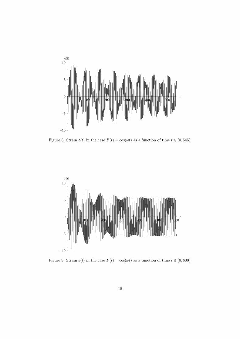
We increase the damping effect by choosing a = 0.55, b = 0.6. The rest of the parametersare: α = 0.45, ω = 1.1. The curve of ε, presented in Figure 9 for smaller times resembles to thecurve of the pulsation (the elastic properties of the material prevail), while later it resembles tothe curve of the forcing function (the viscous properties of the material prevail).
Acknowledgement 7 This research is supported by the Serbian Ministry of Education andScience projects 174005 (TMA and DZ) and 174024 (SP), as well as by the Secretariat forScience of Vojvodina project 114− 451− 2167 (DZ).
References
[1] T. M. Atanackovic, M. Budincevic, and S. Pilipovic. On a fractional distributed-order oscil-lator. Journal of Physics A: Mathematical and General, 38:6703–6713, 2005.
[2] T. M. Atanackovic, S. Konjik, Lj. Oparnica, and D. Zorica. Thermodynamical restrictionsand wave propagation for a class of fractional order viscoelastic rods. Abstract and AppliedAnalysis, 2011:ID975694, 32 pp, 2011.
[3] T. M. Atanackovic, S. Konjik, and S. Pilipovic. Variational problems with fractional deriva-tives: Euler-Lagrange equations. Journal of Physics A: Mathematical and Theoretical,41:095201–095213, 2008.
[4] R. L. Bagley and P. J. Torvik. On the fractional calculus model of viscoelastic behavior.Journal of Rheology, 30:133–155, 1986.
[5] G. Doetsch. Handbuch der Laplace-Transformationen I. Birkhauser, Basel, 1950.
[6] F. Mainardi. Fractional Calculus and Waves in Linear Viscoelasticity. Imperial College Press,London, 2010.
[7] S. G. Samko, A. A. Kilbas, and O. I. Marichev. Fractional Integrals and Derivatives. Gordonand Breach, Amsterdam, 1993.
[8] V. S. Vladimirov. Equations of Mathematical Physics. Mir Publishers, Moscow, 1984.
13

20 40 60 80 100t
-4
-2
0
2
4
ΕHtL
Figure 6: Strain ε(t) in the case F (t) = cos(ωt) as a function of time t ∈ (0, 100).
20 40 60 80 100 120t
-10
-5
0
5
10ΕHtL
Figure 7: Strain ε(t) in the case F (t) = cos(ωt) as a function of time t ∈ (0, 139).
14
100 200 300 400 500t
-10
-5
0
5
10ΕHtL
Figure 8: Strain ε(t) in the case F (t) = cos(ωt) as a function of time t ∈ (0, 545).
100 200 300 400 500 600t
-10
-5
0
5
10ΕHtL
Figure 9: Strain ε(t) in the case F (t) = cos(ωt) as a function of time t ∈ (0, 600).
15