Desaknation, 75 (1989) 15-24 Elsevier Science Publishers B.V., Amsterdam - Printed in The Netherlands

15

AN APPROXIMATE ANALTYICAL SOLUTION FOR THE PERFORMANCE OF REVERSE OSMOSIS PLANTS

A.E.S. Al-Zahrani, M.A. Soliman and I.S. Al-Mutaz

Chemical Engineering Department, King Saud University, P.O.Box 800, Riyadh 11421, Saudi Arabia.

ABSTRACT

Recent developments in membrane technology and appropriate construction

material made reverse osmosis plant attractive for large desalting capacity.

Reserve osmosis showed a growing demand specially in sea water desalting. It

can be considered the optimum process in areas where sufficient electric power

is available at low cost. Due to these reasons, mathematical modeling of

reverse osmosis plants became an important task in the design procedure.

In this paper, the partial differential equations representing the material

and momentum balances inside a hollow fine fiber reverse osmosis model are

discretized by the method of orthogonal collocation. The approximate analyti-

cal solution is obtained by applying the one point collocation method in the

radial and axial direction. This leads to simple expressions for the recovery

and product concentration.

The obtained expressions are compared by the more exact results obtained by

using higher order collocation method. The applicability of these results to

the design and operation of reserve osmosis plants will be disucssed.

PREVIOUS WORK

Dandavati et al(I) presented a model that assumes plug flow of the liquid

in the the shell side in the radial direction. Experiments carried out by

Soltanieh and Gill(2) suggested that the flow could be of the complete mixing

type. The issue is settled by recent experiments of Gill et al who studied the

dynamics of flow in radial flow hollow fiber membranes(2~31. Their study indi-

cate with no doubt that the flow is mixed to a large extent. Since most of the

previous analysis was based on Dandavatiet al work, we give special emphasis in

this work on the effect of the mixing on the steady state behaviour of hollow

fiber membranes and present approximate expressions for the recovery and pro-

duct salt concentration.

oull-9164/89/$03.50 0 Elsevier Science Publishers B.V.

16

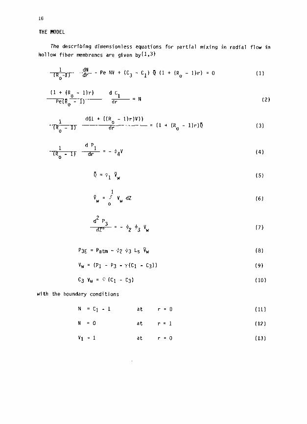
THE MODEL

The describing dimensionless equations for partial mixing in radial flow in

hollow fiber membranes are given by(1,3)

-TR$-)- --$- - Pe NV + (C, - Cl) 4 (1 + (R. - 1)r) = 0 (1)

(1 + (R. - 1)r) d c1

Pe(R, - 1) r=N (2)

(R; - 1)

d((l + ((R. - 1)r)V)) __---_

dr = (1 + (R 0

- l)r)n (3)

d p1 $7 --aF--=-@4V (4)

1 VW = / VW dZ

0

d2 P -a$- = - $2 +3 VW

(6)

(7)

P3E = Patm - $2 $3 Ls 8, (8)

VW = (Pl - P3 - V(Cl - C3)) (9)

c3 vw = 0 (Cl - C3) (10)

with the boundary conditions

N =Cl-1 at r=O (11)

N =0 at r=l (12)

Vl = 1 at r=O (13)

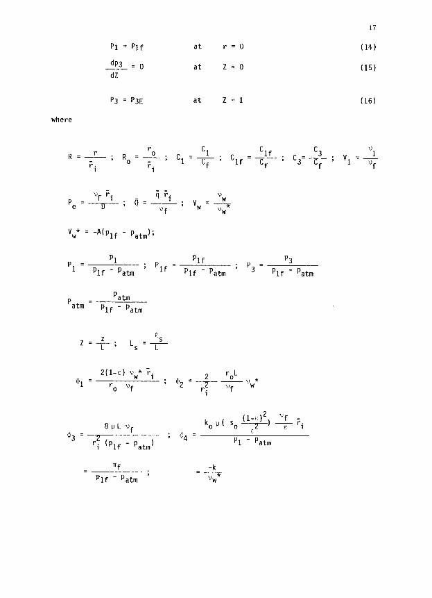
p3 = P3E at 2 =l

where

Pl = Plf at r=O

dP3 = 0

dZ at z=o

r R=&

i: ; Rod!-

i r i

5 ; cl=- Clf c3

Cf ; Clf Cf = ~ ; c3= -

Cf

"f 'i 4 ri Pe=---l)---; q=F

V * = -A(plf - pat”,); W

PI = p1 plf

; Plf = plf - patm ; p3 = plf p3

Plf - Patm - Patm

P P _> =

atm arm

Plf - Patm

61 = 2(1-c) VW* Fi

?lL r

0 "f ; $=+- ___ VW*

ri "f

2 "f -

@3= 2 8ULVf

kop( so +, F 'i

; bq= F

ri 'plf - Patm) p1 - Patm

17

(14)

(15)

(16)

"1 ; vl=T f

nf -k

= Plf - Patm ; =-x

“W

18

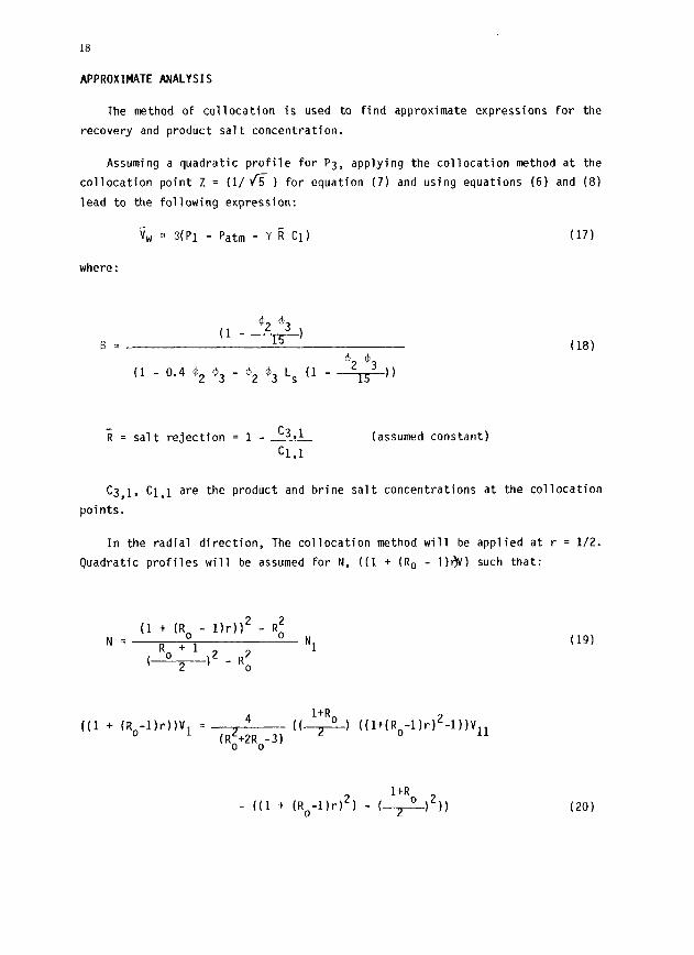
APPROXIMATE ANALYSIS

The method of collocation is used to find approximate expressions for the

recovery and product salt concentration.

Assuming a quadratic profile for P3, applying the collocation method at the

collocation point Z = (I/ 6) for equation (7) and using equations (6) and (8)

lead to the following expression:

Vw = HP1 - Patm - Y R C1)

where:

% $3 B=

(l---l-+

(1 - 0.4 9* e3

R = salt rejection

C3,1, C1,i are the

points.

$2 $3

(18)

- Qi* 93 Ls (1 - --f5-H

= 1 _ C3,1

Cl,1

(assumed constant)

product and brine salt concentrations at the collocation

ied at r = l/2. In the radial direction, The collocation method will be appl

Quadratic profiles will be assumed for N, ((1 + (R, - 11r)y) such that:

N= (’ + (R. - l)r112 - RE

R. + 1 ( 2 12-R;

Nl

((1 + (Ro-l)r))Vl = 2 4 l+R,

(Ro+2Ro-3) (b-1 ((l+(Ro-l)r)2-l))V,l

ltRo 2 - ((1 + (Ro-llrl*) - (-2-----) 11

(171

(19)

(20)

19

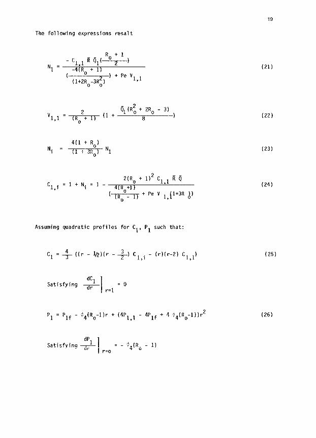
The following expressions resalt

N1 =

R. + 1 - Cl,1 R 01'-7j----'

( -4(Ro + 1)

(1+2Ro-3R;) ) + Pe vlyl

2 __

'l,i = 1 + Ni = l-

2(R, + 1) Cl,1 R 9

4(Ro+l)

( (R. _ 1) + PI? ” l,j1+3R A)

2 $(R; + ZR, - 3)

"1,l = (R. + 1) (' + 8 )

Ni = 4(1 + Ro)

(1+3Ro) N1

Assuming quadratic profiles for Cl, Pl such that:

Cl = + ((r - l/il)(r - -+-I Cl i - (r)(r-2) Cl 1) , ,

Satisfying dC1

F I r=l = 0

p1 = Plf - @4(Ro-l)r + (4P1,l - 4Plf + 4 $4(Ro-l))r 2

(21)

(22)

(23)

(24)

(25)

(26)

dP1 Satisfying F I r=o

= - a4(Ro - 1)

20

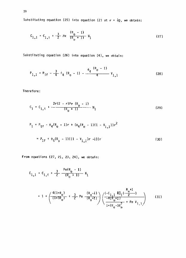
Substituting equation (25) into equation (2) at r = 1/2, we obtain:

Cl,1 = ‘1.i + -+- Pe :i” i :; Nl

0

Substituting equation (26) into equation (4), we obtain:

p1,1 = b4 (Ro - 1)

Plf - _b @4 (R. - 1) - -4 '$1

Therefore:

Cl = Cl i + 2r(2 - r)Pe (R. - 1)

I IRo + l) Y

p1 = Qf - @4(Ro - 1)r + (04(Ro - I)(1 - Vl l))r2 ,

= Plf + @4(Ro - l)((l - v 1 1))” -1))r ,

From equations (27, 21, 23, 24), we obtain:

Cl,1 3

= cl,i + 2 Pe(Ro - 1)

(R. + 1) Nl

(27)

(28)

(29)

(30)

(31)

Therefore:

c1,1 1 =

(Ro-1)

0)

R 01 (Ro+l)

2 1+ - +

( 0’

( 1+2Ro _ 3Rz) + Pe “Ll

21

(32)

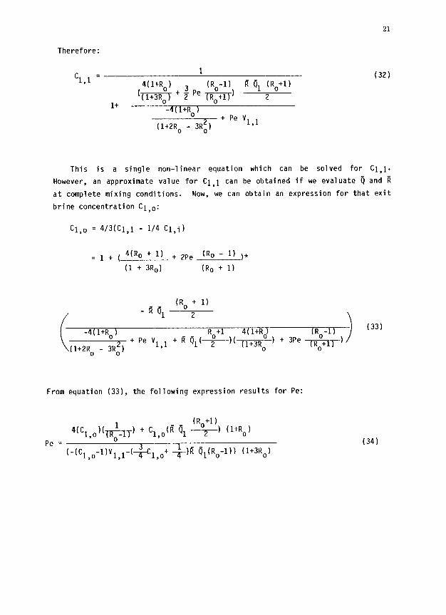
This is a single non-linear equation which can be solved for Cl,l.

However, an approximate value for Cl,1 can be obtained if we evaluate q and R

at complete mixing conditions. Now, we can obtain an expression for that exit

brine concentration CI,~:

Cl,0 = 4/3(Cl,l - l/4 Cl,i)

= 1 + ( 4(Ro + 11 + 2Pe (Ro - 1’ ,A

(1 + 3Ro) (R. + 1)

l=i 0, (R. + 1’

2

-4(1+Ro) Ro+l 4( l+Ro) ( (33)

(l+2Ro _ 3Ri) + Pe “1.1 + Ii VT--)((liRo) + 3Pe .-&-)

From equation (33), the following expression results for Pe:

Pe =

4(Cl,o)(& + Cl,o(R 01 0) (l+Ro)

(-(Cl,o-l)“l,l-(-&o+ +)R $(R,-1)) (1+3Ro) (34)

22

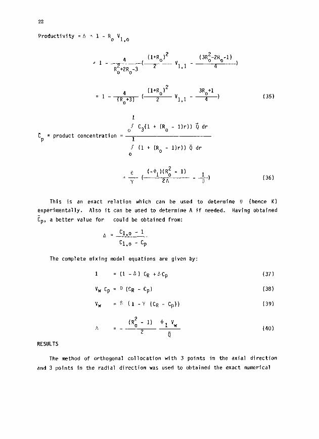
Productivity = A = 1 - R. VI o ,

=I_ 4 (1+Ro12 (3Rz-2Ro-1)

R;+2Ro-3 +F---- vl,l --4-)

(1+Ro12

=1--g+ 2

3R,+l

Yl,l - -7-l (351

1

0 I C3(l + (R. - 1)r1) q dr

cp = product concentration = 1

/ (1 + (R. - 1)r)) q dr 0

(36)

This is an exact relation which can be used to determine f3 (hence K)

experimentally. Also it can be used to determine A if needed. Having obtained

cp, a better value for could be obtained from:

* = Cl,0 - 1

Cl,0 - cp

The complete mixing model equations are given by:

1 = (1 -A) CR +ACp

v, Cp = o (CR - Cp)

VW = 6 (1 -y (CR - Cp))

A =_ (R; - 1) 41 VW

2 0

RESULTS

The method of orthogonal collocation with 3 points in the axial direction

and 3 points in the radial direction was used to obtained the exact numerical

(37)

(38)

(39)

(40)

23

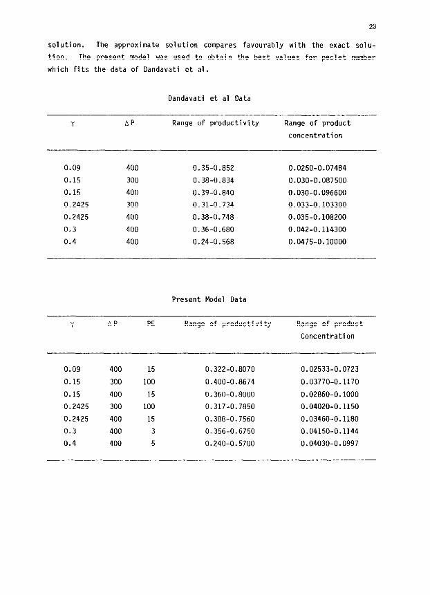
solution. The approximate solution compares favourably with the exact solu-

tion. The present model was used to obtain the best values for peclet number

which fits the data of Oandavati et al.

Oandavati et al Data

Y AP Range of productivity Range of product

concentration

0.09 400 0.35-0.852 0.0250-0.07484

0.15 300 0.38-0.834 0.030-0.087500

0.15 400 0.39-0.840 0.030-0.096600

0.2425 300 0.31-0.734 0.033-0.103300

0.2425 400 0.38-0.748 0.035-0.108200

0.3 400 0.36-0.680 0.042-0.114300

0.4 400 0.24-0.568 0.0475-0.10000

Present Model Data

Y AP PE Range of productivity Range of product

Concentration

0.09 400 15 0.322-0.8070 0.02533-0.0723

0.15 300 100 0.400-0.8674 0.03770-0.1170

0.15 400 15 0.360-0.8000 0.02860-0.1000

0.2425 300 100 0.317-0.7850 0.04020-0.1150

0.2425 400 15 0.388-0.7560 0.03460-0.1180

0.3 400 3 0.356-0.6750 0.04150-0.1144

0.4 400 5 0.240-0.5700 0.04030-0.0997

24

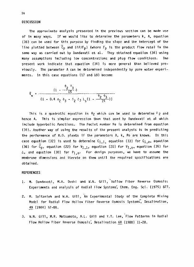
DISCUSSION

The approximate analysis presented in the previous section can be made use

of in many ways. If we would like to determine the parameters k, A, equation

(36) can be used for this purpose by finding the slope and the intercept of the

line plotted between C, and (AP/Fp) (where Fp is the product flow rate) in the

same way as carried out by Dandavati et al. They obtained equation (34) using

many assumptions including low concentrations and plug flow conditions. The

present work indicate that equation (34) is more general than believed pre-

viously. The parameter A can be determined independently by pure water experi-

ments. In this case equations (17 and 18) become

b2 $3

VW = (l----i+

(1 - 0.4 b2 @3 - $2 a3 L&l - $2 93

--K-”

This is a quadratic equation in $2 which can be used to determine $2 and

hence A. This is simpler expression than that used by Dandavati et al which

include hyperbolic functions. The Peclet number Pe is determined from equation

(34). Another way of using the results of the present analysis is in predicting

the performance of R.O. plants if the parameters A, k, Pe are known. In this

case equation (32) is used to determine Cl,l, equation (33) for CI,~, equation

(36) for cp, equation (22) for V1,1, equation (20) for VI,~. equation (35)

A, and equation (30) for PI,~. For design purposes, we have to assume

membrane dimensions and iterate on them until the required specifications

obtained.

for

the

are

REFERENCES

1. M. Dandavati, M.R. Doshi and W.N. Gill, *Hollow Fiber Reverse Osmosis:

Experiments and analysis of Radial Flow Systems'; Chem. Eng. Sci. (1975) 877.

2. M. Soltanieh and W.N. Gill, 'An Experimental Study of the Complete Mixing

Model for Radial Flow Hollow Fiber Reverse Osmosis System;, Desalination,

49 (1984) 57-88. -

3. W.N. Gill, M.R. Matsumoto, A.L. Gill and Y.T. Lee,'Flow Patterns in Radia

Flow Hollow Fiber Reverse Osmosis’: Desalination 68 (1988) 11-28. -