a large gem detector prototype

Universita degli Studi di SienaFACOLTA DI SCIENZE MATEMATICHE, FISICHE E NATURALI

Corso di Laurea Triennale in Fisica e Tecnologie Avanzate

Tesi di Laurea

18 Aprile 2011

A Large GEM detector prototype

Test-beam results and analysis

Candidato:Elena Graverini

Relatore:Prof. Nicola Turini

Anno Accademico 2009–2010

Contents

Abstract . . . . . . . . . . . . . . . . . . . . . . . . . . . . . . . . . 5

Sommario . . . . . . . . . . . . . . . . . . . . . . . . . . . . . . . . 7

Acknowledgements . . . . . . . . . . . . . . . . . . . . . . . . . . . 9

1 The prototype: a large GEM 11

1.1 GEM detectors . . . . . . . . . . . . . . . . . . . . . . . . . . 11

1.2 Choice of the gas . . . . . . . . . . . . . . . . . . . . . . . . . 14

1.3 A large triple GEM detector . . . . . . . . . . . . . . . . . . . 19

1.3.1 Gain curve . . . . . . . . . . . . . . . . . . . . . . . . . 22

2 Readout electronics 25

2.1 VFAT2 readout chip . . . . . . . . . . . . . . . . . . . . . . . 25

2.2 Turbo readout card . . . . . . . . . . . . . . . . . . . . . . . . 29

2.3 O-beam threshold scan . . . . . . . . . . . . . . . . . . . . . 30

3 Experimental setup 33

3.1 The test-beam facility . . . . . . . . . . . . . . . . . . . . . . 33

3.2 The telescope . . . . . . . . . . . . . . . . . . . . . . . . . . . 34

3.3 Data analysis system . . . . . . . . . . . . . . . . . . . . . . . 35

3.3.1 Hits, clusters and tracks . . . . . . . . . . . . . . . . . 35

3.3.2 Reconstructing the beam prole . . . . . . . . . . . . . 37

4 On-beam tests 41

4.1 Eciency of the tracker . . . . . . . . . . . . . . . . . . . . . 41

3

4 CONTENTS

4.2 High voltage scan . . . . . . . . . . . . . . . . . . . . . . . . . 42

4.3 Threshold scan . . . . . . . . . . . . . . . . . . . . . . . . . . 46

4.4 Timing scan . . . . . . . . . . . . . . . . . . . . . . . . . . . . 51

4.5 Behaviour with hadron beam . . . . . . . . . . . . . . . . . . 56

5 Remarks 59

5.1 (In)homogeneity of the prototype . . . . . . . . . . . . . . . . 59

5.1.1 Critical chamber zones . . . . . . . . . . . . . . . . . . 59

5.1.2 Eects of the dierent pad dimensions . . . . . . . . . 63

5.2 Eciency radius lenght: noise checks . . . . . . . . . . . . . . 66

5.3 Analysis algorithms: cuts . . . . . . . . . . . . . . . . . . . . . 70

6 Conclusions 73

6.1 Quality of the large GEM prototype . . . . . . . . . . . . . . . 73

6.2 Large GEMs for TOTEM and CMS . . . . . . . . . . . . . . . 74

Appendix A ROOT analysis routines 77

A.1 Data reconstructing algorithms . . . . . . . . . . . . . . . . . 77

A.2 Scan-specic algorithms . . . . . . . . . . . . . . . . . . . . . 85

List of Figures 107

List of Tables 111

Listings 113

Bibliography 115

Abstract

My thesis presents the tests performed on a new Gas Electron Multiplier

detector, capable of revealing electromagnetic-interacting particles. It is a

large area prototype, developed using innovative techniques that allow for

the splicing of several small GEM foils together to obtain a single large foil.

A single-mask etching technique was used to overcome alignment problems.

The tests were performed at the CERN laboratories in Genève, in order to

verify the prototype eciency. It was also necessary to test the compatibility

of a high-capacitance readout plane with the front-end electronics now used

by the TOTEM experiment at LHC. The prototype was indeed conceived

as a possible future replacement for the CSCs (Cathode Strip Chambers)

TOTEM has been employing so far.

In this thesis, I will report on the manufacture of the detector in detail,

as well as on the preliminary gain and noise tests. The readout electronics

and the test beam setup will also be described. I will then give a thorough

account of the test beam results in order to provide a complete character-

ization of the prototype. Finally, I will go through some of the algorithms

exploited in the data analysis process. The pieces of code I wrote myself are

collected in an Appendix.

The results we achieved will be then compared with those expected by

previous generation GEM detectors. I will suggest some opportunities for

further improvements, especially with regard to the better time resolution

which will be needed, in the near future, in order to meet the expected LHC

higher working rate.

5

Sommario

La mia tesi presenta la serie di test eseguiti su un nuovo rivelatore di parti-

celle di tipo Gas Electron Multiplier, in grado di rivelare fotoni e particelle

cariche. Si tratta di un prototipo di grande area, realizzato con tecniche in-

novative che permettono di unire più fogli GEM di dimensioni minori in un

solo piano e di evitare problemi di allineamento in fase di foratura.

I test sono stati eseguiti nei laboratori CERN di Ginevra allo scopo di

vericare le prestazioni del prototipo. Inoltre, era necessario testare la com-

patibilità di un piano di readout ad alta capacità con l'elettronica attualmen-

te in uso nell'esperimento TOTEM presso LHC: il prototipo è stato infatti

concepito nell'ottica di una futura sostituzione delle attuali camere CSC (Ca-

thode Strip Chamber) di TOTEM con rivelatori a GEM di grande area.

Esporrò in dettaglio il processo di costruzione del prototipo, i test pre-

liminari di guadagno e l'analisi del rumore; verrà descritta l'elettronica di

readout, per poi passare all'allestimento dei test su fascio di particelle. Esa-

minerò quindi i risultati ottenuti in questa fase, nell'ottica di un'integrale

caratterizzazione del rivelatore. Spiegherò inoltre il funzionamento di alcuni

degli algoritmi utilizzati per l'analisi dei dati raccolti durante il test beam.

In appendice ho raccolto, in particolare, quelli che io stessa ho elaborato.

I risultati ottenuti verranno inne confrontati con le prestazioni attese dai

rivelatori GEM di precedente generazione, e suggerirò le ulteriori migliorie che

possono essere apportate in futuro, soprattutto per aumentarne la risoluzione

temporale in vista del previsto incremento della frequenza di lavoro di LHC.

7

Aknowledgements

This thesis could not have been written if I had not received a grant, from

the Siena Department of Physics, TOTEM and the INFN, to spend two

months at CERN, where I met researchers who introduced me to experimen-

tal physics and actively involved me in their work: Eraldo Oliveri, Mirko

Berretti, Stefano Lami and Nicola Turini, from TOTEM. In particular, I

wish to thank Eraldo for all the precious help he gave me, both during the

lab tests and while I was writing down my thesis. I was also directly involved

in the RD51 research group, led by Leszek Ropelewski, where I had the luck

to meet Matteo Alfonsi and Gabriele Croci. My deepest gratitude therefore

goes to all of them. Not only did they teach me how to contribute to a scien-

tic research, but they also made my stay at CERN entertaining and friendly.

I am also deeply grateful to prof. Emilio d'Emilio and prof. Maria Imma-

colata Loredo. It is because of their intriguing teaching that, after all this

exciting lab work, I am still doubtful whether I should pursue experimental

or theoretical physics.

During my studies in Siena, the neverending enthusiasm of Alessandro

Marchini and prof. Vincenzo Millucci made me realize how stimulating and

even amusing is to devote one's free time to scientic activities. They intro-

duced me to astronomy, and infected me with their passion for transmitting

love for science to younger people and prospective university students. They

demonstrated to me that university life should consist of both curricular and

extra-curricular activites, and that often the best incentives to learn come

from the latter ones.

Last but not least, a heartfelt thanks to the people who have been so

close to me during these years - Salvo, Arianna, and all the other friends.

9

Chapter 1The prototype: a large GEM

1.1 GEM detectors

High-energy physics studies the kinetic features of particles and their inter-

actions by using detectors which reveal, for example, the product of collisions

in accelerators, or detect cosmic rays. Dierent kinds of detectors are used

to reveal dierent properties of the particles themselves: kinetic energy, mo-

mentum, charge, mass and even their internal structure.

Gas ionization detectors can reveal high-rate electromagnetic-interacting

particles. If the incident photon or charged massive particle has enough en-

ergy to ionize one atom of gas inside the detector, the ux of ion-electron

pairs will be amplied; this will generate a current pulse for each event. Each

signal can be revealed by a copper anode and can then be sent to electronic

data acquisition (DAQ) systems.

Gaseous detectors can produce an avalanche multiplication of the signal

by accelerating (through an electric eld) the rst electrons produced by the

incident particle, so that they release more pairs. Gas electron multipliers

(GEMs) work according to such principle. GEM foils consist of two thin

copper layers, with a kapton foil between them. Small holes are made in a

regular pattern through these foils, via chemical processes such as photoli-

11

12 CHAPTER 1. THE PROTOTYPE: A LARGE GEM

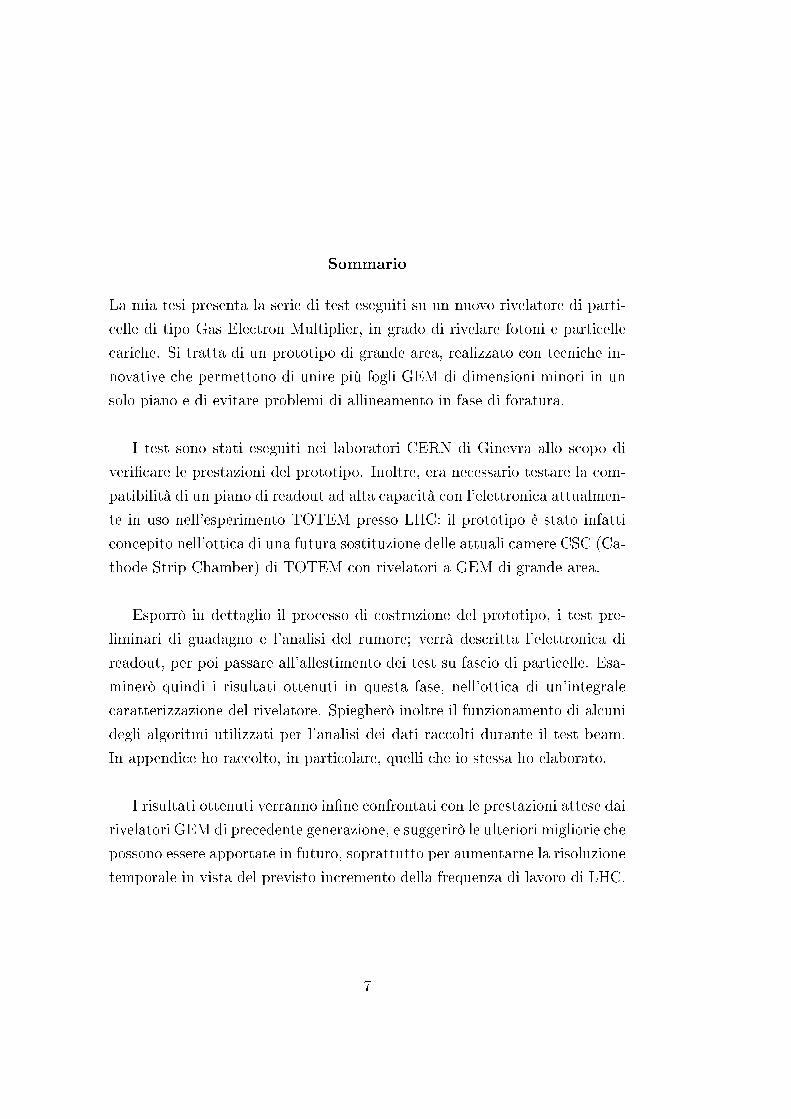
(a) Draft of a single-GEM detector (b) Hole pattern

Figure 1.1: Schematic outline of a single-GEM detector and, on the right, view of thehole pattern in a GEM foil

tography and acid etching (Figure 1.1(b)).

A potential is then applied between the two copper layers (anode and

cathode) in order to put the GEM foil into operation; this will create a high

electric eld through the holes:

E =V

d

where E is the electric eld, V is the voltage and d is the distance between

the anode and the cathode. Since the kapton foil is very thin (around 25µm),

but it can resist high electric elds1, the potential between GEM electrodes

can be as high as 500÷ 600V .

A GEM-based detector consists of one or more GEM foils laid, as shown

in Figure 1.1(a), between a copper foil (cathode) and a readout plane (anode).

A drift eld is applied to drive electrons from the cathode drift foil to

the GEM. An amplication voltage between the copper layers of every GEM

foil accelerates the electrons, producing avalanche multiplication. Finally, an

1Kapton is a plastic polyimide created by DuPont, whose molecular structure remainsstable in a wide range of temperatures. It was dicovered to be very radiation-hard, and iscommonly used for its good insulating power [9].

1.1. GEM DETECTORS 13

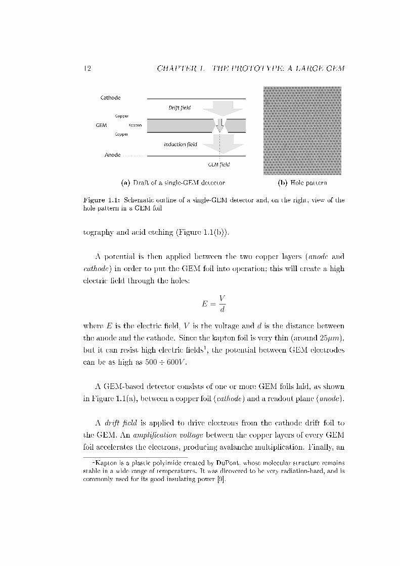
Figure 1.2: Draft cross-section of a triple GEM detector [7]

induction eld leads them from the GEM bottom layer to the readout plane.

In the case of a multiple GEM detector, transfer elds drive electrons from

a GEM foil to the next.

More GEM foils can be inserted as a cascade in a single detector. This

allows to reduce the discharge probability, as we can set quite a low multipli-

cation potential between the electrodes of each foil. The discharge probability

is indeed a function of charge density inside the GEM holes. In this congura-

tion, the typical gains of each GEM are around G ' 15÷30; for a triple-GEM

detector this leads to a total gain of the order of magnitude of several thou-

sands (for example, for TOTEM T2 telescope chambers G ' 8, 000).

Figure 1.2 shows the usual cross section of a triple GEM chamber. Ed,

Et and Ei stand for the drift, transfer and induction elds, respectively. Gap

depths gd, gt and gi are customizable. In particular, stretching the drift gap

allows to increase the number of primary ionizations, but on the other hand

it decreases the time performance. Specic application requirements deter-

mine the most tting chamber geometry.

The detector being analyzed in this thesis is a triple GEM chamber,

whose gaps were set as in Table 1.1 on the next page; Table 4.1 on page 42


Drift gap Transfer gap 1 Transfer gap 2 Induction gap

gd = 3mm gt1 = 2mm gt2 = 2mm gi = 2mm

EMINd = 2.7kV

cmEMINt1

= 4.0kVcm

EMINt2

= 4.0kVcm

EMINi = 4.0kV

cm

EMAXd = 3.0kV

cmEMAXt1

= 4.4kVcm

EMAXt2

= 4.4kVcm

EMAXi = 4.4kV

cm

Table 1.1: Large GEM gap depths and electric elds

shows instead the gain values we reached during the tests conducted on this

chamber. Table 1.1 also shows the range of electric elds we applied to each

gap during the test-beam.

1.2 Choice of the gas

Interaction of incident charged particles or photons with matter is the basis

on which Gas Electron Multiplier detectors work. A gas mixture ows in-

side the detector, or is sealed in it; its components are chosen according to

their ionization potential, ion transport characteristics and ageing properties.

In most cases, only the electromagnetic (Coulomb) interaction is used for

detection purposes. Strong and weak interactions are by far less probable,

and in any case they cannot be revealed in a GEM. Coulomb interactions

result in excitation and ionization of the gas molecules, and in negligible

part in bremsstrahlung, erenkov and transition emission of radiation. In

particular, noble gases do not present many energy dissipation modes: they

can only be excited through photon absorption (and consequent emission).

The absence of the many non-ionizing dissipation modes, which are typical

of polyatomic molecules, is then the reason for which noble gases are chosen

as main component in any gaseous detector. Ionization is indeed the main

mode of interaction occurring in noble gases, so electron avalanche multipli-

cation is eased. On the other hand, specic experimental requirements often

oblige the use of compounds containing polyatomic molecules.

1.2. CHOICE OF THE GAS 15

As already said, excited noble gases can only return to the ground state

through emission of a photon. Argon, for example, releases photons with

energy Eγ ≥ 11.6eV , that are themselves able to ionize copper atoms of the

GEM anodes (whose ionization potential equalsWi = 7.7eV ). Argon positive

ions drift instead towards the cathode, where they recombine extracting an

electron and causing secondary photons or electrons to be emitted as energy

balancement. Both these processes result in spurious avalanches; even with

a moderate gain, detectors may therefore experience frequent discharges. In

addition, spurious signals such those would aect the space and time resolu-

tion.

We thus need to add a percentage of so-called quenchers to the gas

mixture. Hydrocarbons, alcohols and freons are examples of the most used

quenchers. Their complex molecules feature a large number of non-radiative

excitation modes and allow photon absorption in the range of energy of those

emitted by argon. Elastic collisions and quencher dissociation into simpler

molecules dissipate the energy in excess, ensuring stability of operation of

the detector. Despite this, attention must be paid to the process through

which polyatomic ionized molecules neutralize. In fact, if radicals use to

combine together to form larger polymers, precipitate and accumulate inside

the chamber, that might speed up its ageing process.

The expression obtained by Bethe and Bloch for the average dierential

energy loss due to Coulomb interactions is:

dE

dx= −2πNz2e4

mc2Z

A

ρ

β2

(ln

2mc2β2EMI2 (1− β2)

− 2β2

)where N is the Avogadro number, Z, A, ρ and I are the atomic number,

atomic mass, density and average ionization potential of the medium, z and

β are the atomic number and speed in units of c of the projectile [14]. EMrepresents the maximum transferable energy. Figure 1.3(a) on page 17 shows,

as an example, the contributions of various processes to the total energy loss


of muons µ+ in copper.

Above a kinetic energy of the order of magnitude of a few hundred

MeV every particle lies in the minimum ionization region of the curve (Fig-

ure 1.3(b) on the next page) and release on average 2MeV · cm2

g. At those

energy levels, which is the most common situation in high-energy physics,

the particles are called MIPs.

A number of ionization clusters are created on the passage of a MIP

through the drift gap of the detector. Drift and transfer elds drive the

ejected electrons through the GEM foils, where they are accelerated and

cause more ionizations. The induction eld attracts the electron avalanche

on the anode, where each drifting electron turns into a current signal of in-

tensity I =e

∆tdriftand duration ∆tdrift =

livdrift

, where li is the thickness of

the induction gap and vdrift is the drift velocity of electrons (vdrift depends

on the voltage applied to the gaps).

The total signal induced by an incident particle is given by the superpo-

sition of the signals produced by the primary ionization electrons (the ones

extracted directly by the MIP crossing the drift region) multiplied by the

total gain factor. The signals coming from dierent primary electrons will be

detected at dierent times, because the spacial distribution of the ionization

clusters can be as wide as the drift gap. The time resolution of the detector

is determined by the space distribution of each ionization cluster, which fol-

low the Poisson law, with a sigma σ(t) ∝ 1

n · vdrift(where n is the average

number of primary ionization clusters) [7].

In order to optimise the time resolution of a detector it is therefore neces-

sary to maximize the drift velocity, and the number of primary clusters, using

gas mixtures with a large average atomic number. The gas inside the detec-

tor should allow a compromise between these two features and the minimum

possible loss of eciency as compared to a noble gas. A higher drift velocity

1.2. CHOICE OF THE GAS 17

(a) An example of −dEdx

of projectiles in a medium according to the Bethe-

Bloch formula, from [1]. Energy loss is plotted as a function of βγ =p

Mc

(b) Energy loss in air for dierent particlesas a function of their energy, from [14]

Figure 1.3: Energy loss due to Coulomb interaction of particles in media


Figure 1.4: Drift velocity of electrons in several argon-isobutane mixtures

may be obtained by either increasing the drift, transfer and induction elds

or adding a percentage of polyatomic molecules (a full explanation of this

topic can be found in [14]).

The measurements presented in this text were performed using two gas

mixtures: Ar/CO2 70/30 and Ar/CO2/CF4 60/20/20, with CO2 and CF4

as quenchers. The choice of CF4 for the last set of tests was driven by its

good timing characteristics, already veried by the authors of [7]; moreover,

with respect to methane and other hydrocarbons, it is safer. CF4 is indeed

non-ammable, non-toxic and non-corrosive either for metal or plastic ma-

terials. It might only be harmful if it comes into contact with hydrogen, as

this would allow for the formation of hydrouoric acid HF. Ar/CO2 70/30 is

instead the standard gas mixture in use at TOTEM and other experiments.

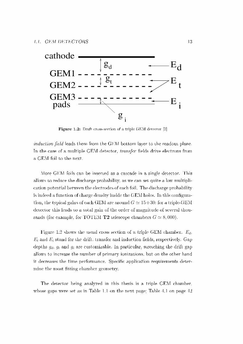
Figure 1.5 on the facing page shows the dierences between Ar/CO2 70/30

and Ar/CO2/CF4 60/20/20 as found in literature; our measurements will

be presented in Chapter 4.2 on page 42 for what concerns the relationship

between GEM elds and gain, and in Chapter 4.4 on page 51 I will show and

discuss the timing tests we performed.

1.3. A LARGE TRIPLE GEM DETECTOR 19

(a) Electron drift velocity (b) Triple GEM gain

Figure 1.5: Properties of dierent gas mixtures. The measurements were done for atriple GEM detector with elds Ed = Et = 3kV

cm [7]

1.3 A large triple GEM detector

At CERN, a prototype triple GEM detector (Large GEM, abbreviated LG)

was built2 with an active area of about 2000cm2 using 66 · 66cm2 kapton

copper-clad foils [13]. Two innovative techniques were used to manufacture

this detector: single-mask etching and GEM foils splicing.

GEM foils are manufactured through the same photolitographic processes

used to produce common printed circuit boards. Tipically, small GEMs are

etched on both sides to obtain symmetric holes. However, it can very un-

comfortable to align masks when the GEM foil dimensions grow. Due to

the very large area of this prototype, it was necessary to renew a single-

mask etching technique. As shown in Figure 1.6 on the next page, after the

top copper layer is etched, a basic mixture containing potassium hydroxide

(KOH, which etches isotropically) and ethylene diamine (C2H4(NH2)2, which

etches anisotropically) was used to make the holes in the polymide material

(Kapton). An anisotropic etcher was needed to keep the holes aspect ratio

large, dened asdepth

width.

2Design by S. D. Pinto, CERN, on behalf of RD51 group.


Figure 1.6: Comparison of the standard double-mask and the new single-mask GEMetching procedures [13]

The bottom copper layer was then etched on both sides, using the holes

in the kapton as masks, dipping the whole foil in an acidic etchant mixture

in order to nalize the holes and to reduce the thickness of the electrodes.

When the detector was built, suppliers of the GEM foils base material

could only oer 50÷70cm wide rolls. A 66x66cm2 foil was cut crosswise, and

the two halves were spliced together by covering the junction with a 25µm

Kapton adhesive substrate. The glue polymerized by baking.

Rate capability tests demonstrated that the chamber performance re-

mains unaected except for the 2mm wide seam zone [12]. In addition, a

3.5mm wide plastic spacer was placed, in the triple GEM detector we tested,

exactly over the foils junction areas, covering them totally. This made it

impossible to recognize the loss of eciency due to the seam.

Foreseeing the possibility of discharges, the cathode electrodes are seg-

mented and connected to the power supply via 10MΩ resistors in order to

reduce their energy storage. A compact divider board supplies high voltage,


(a) View of the prototype (b) Layout of the GEM foils sectors

Figure 1.7: A photo and a scheme of the large area triple GEM prototype

(a) Divider board (b) Readout plane, made of pads

Figure 1.8: A view of the compact divider board, and a sketch of the pad-based readoutshowing the beam-tested regions


in order to make it easier to debug the circuit if needed. Since the board

was not designed to handle such high voltages, groups of pins were connected

together and alternated with groups of oating strips (see Figure 1.8(a) on

the preceding page).

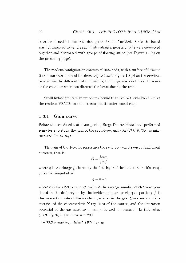
The readout conguration consists of 1024 pads, with a surface of 0.25cm2

(in the narrowest part of the detector) to 6cm2. Figure 1.8(b) on the previous

page shows the dierent pad dimensions; the image also evidences the zones

of the chamber where we directed the beam during the tests.

Small hybrid printed circuit boards bound to the chips themselves connect

the readout VFAT2s to the detector, on its outer round edge.

1.3.1 Gain curve

Before the scheduled test beam period, Serge Duarte Pinto3 had performed

some tests to study the gain of the prototype, using Ar/CO2 70/30 gas mix-

ture and Cu X-Rays.

The gain of the detector represents the ratio between its output and input

currents, that is:

G =IOUTq ∗ f

where q is the charge gathered by the rst layer of the detector. In this setup

q can be computed as:

q = n ∗ e

where e is the electron charge and n is the average number of electrons pro-

duced in the drift region by the incident photon or charged particle; f is

the interaction rate of the incident particles in the gas. Since we know the

energies of the characteristic X-ray lines of the source, and the ionization

potential of the gas mixture in use, n is well determined. In this setup

(Ar/CO2 70/30) we have n ' 290.

3CERN researcher, on behalf of RD51 group


Divider HV [kV]3.6 3.8 4.0 4.2 4.4

LG

Gai

n

310

410

510

LG left sideLG right side [nA-meter wrong offset]Exponential fit (left)

Divider current [uA]660 680 700 720 740 760 780 800 820

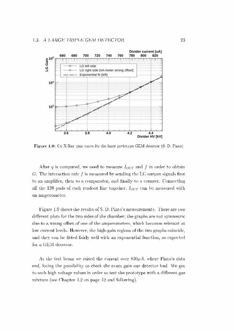
Figure 1.9: Cu X-Ray gain curve for the large prototype GEM detector (S. D. Pinto)

After q is computed, we need to measure IOUT and f in order to obtain

G. The interaction rate f is measured by sending the LG output signals rst

to an amplier, then to a comparator, and nally to a counter. Connecting

all the 128 pads of each readout line together, IOUT can be measured with

an amperometer.

Figure 1.9 shows the results of S. D. Pinto's measurements. There are two

dierent plots for the two sides of the chamber; the graphs are not symmetric

due to a wrong oset of one of the amperometers, which becomes relevant at

low current levels. However, the high-gain regions of the two graphs coincide,

and they can be tted fairly well with an exponential function, as expected

for a GEM detector.

At the test beam we raised the current over 830µA, where Pinto's data

end, losing the possibility to check the exact gain our detector had. We got

to such high voltage values in order to test the prototype with a dierent gas

mixture (see Chapter 4.2 on page 42 and following).


For this and other reasons, a new gain curve is required, which will touch

high divider current values and will check the uniformity of the detector

within its left and right sides.

Chapter 2Readout electronics

2.1 VFAT2 readout chip

VFAT2 is the front-end electronics developed for the TOTEM experiment

at the LHC. This ASIC (Application Specic Integrated Circuit) converts

the signals from the detectors into digital data through an amplier-shaper-

comparator chain.

The readout chips used during the test-beam were VFAT2 chips as well,

since one of the aims of the test was a compatibility check between large ca-

pacitance pad-based readout systems and the TOTEM front-end electronics.

VFAT2 features a transimpedance preamplication step (VOUT ∝ IIN),

whose output is sent to a shaper, and then compared to a customizable

threshold potential. The latter is programmable in terms of VFAT2 DAC

step bins1. A feature named TrimDAC allows us to set dierent thresholds

for each channels, optimizing therefore the process of data acquisition even

in noisy environments; however, we did not use this feature during the tests.

The monostable block then synchronizes the output of the comparator,

1Each VFAT2 DAC step bin corresponds to 3.3mV , that is an input charge of about0, 045fC ≈ 281e−.

25

26 CHAPTER 2. READOUT ELECTRONICS

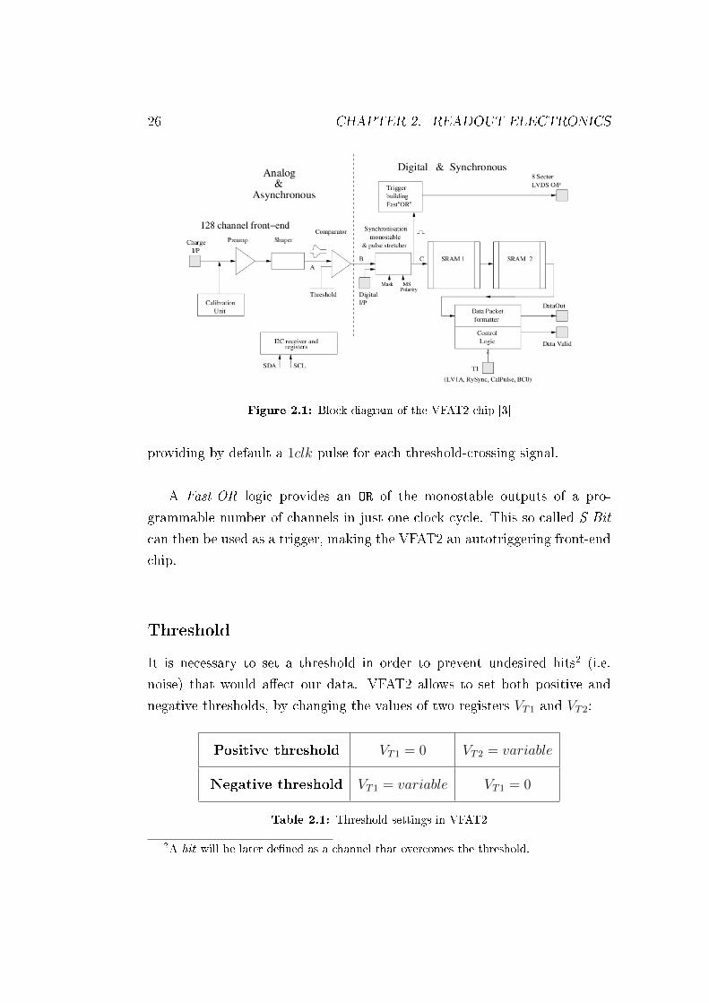
Figure 2.1: Block diagram of the VFAT2 chip [3]

providing by default a 1clk pulse for each threshold-crossing signal.

A Fast-OR logic provides an OR of the monostable outputs of a pro-

grammable number of channels in just one clock cycle. This so-called S-Bit

can then be used as a trigger, making the VFAT2 an autotriggering front-end

chip.

Threshold

It is necessary to set a threshold in order to prevent undesired hits2 (i.e.

noise) that would aect our data. VFAT2 allows to set both positive and

negative thresholds, by changing the values of two registers VT1 and VT2:

Positive threshold VT1 = 0 VT2 = variable

Negative threshold VT1 = variable VT1 = 0

Table 2.1: Threshold settings in VFAT2

2A hit will be later dened as a channel that overcomes the threshold.

2.1. VFAT2 READOUT CHIP 27

(a) Fast-OR logic combining the monostable outputs to provide a trigger signalwithin one clock cycle [2]

(b) Signal shaping for MSPL = 1clk [5]

Figure 2.2: Fast trigger and shaping features of VFAT2 chips


The threshold is then computed as VTH = VT2 − VT1.

Most of our scans were run at th = −60ds (where ds stands for VFAT2

DAC step bin). Threshold scans were performed as well, to see at what level

the noise starts to become signicant: see Chapter 4.3 on page 46.

Latency

Given a trigger signal, we dene latency the number of SRAM locations the

chip has to go back in order to read the digital output of the event corre-

sponding to that trigger. It is measured in clock periods, as it represents the

elapsed time between the arrival of the trigger and the preceding storage of

the corresponding event in the VFAT2 SRAM.

The latency of our setup was found to be lat = 17clk when working with

Ar/CO2 70/30, and lat = 18clk when working with Ar/CO2/CF4 60/20/20.

Monostable settings

A signal can have either a thin or a large time distribution of charge (jitter

eect); the preamplier stage preserves itsamplitude

widthratio. The monostable

block allows to stretch its output pulse, which can be programmed to be as

long as 1 to 8 clock periods. Stretching the monostable pulse generally de-

creases the time performance, as a subsequent signal may cross the threshold

while the monostable output is still high. This would result in a single pulse

instead of two, which would stay high for n more clock cycles after the last

threshold crossing, 1 ≤ n ≤ 8.

However, stretching the monostable pulse allows us to nd out whether

two or more pulses are to be recognized as originated by the same event. Two

undesired eects may happen indeed, which are countered by stretching the

monostable output:

2.2. TURBO READOUT CARD 29

• Timewalk: adjacent channels may be hit with dierent intensity (e.g.

an electron avalanche falls over two adjacent pads): in this case, the

channels which gather less charge may cross the threshold later than

the other ones;

• Jitter: primary ionization clusters may be produced anywhere in the

drift region, which has a signicant thickness. Electrons released by

the same incident particle at dierent heights in the drift region will

thus reach the anode at dierent times; for a 3mm thick gap, and elds

like those of Table 1.1 on page 14, the arrival time spread of drifting

electrons can reach 60ns.

By stretching the monostable we can then synchronize several detectors

being crossed by the same particle. In addition, a single latency value would

allow us to retrieve the signals produced by all the tracks, despite possible

timewalk-jitter delays.

2.2 Turbo readout card

We used two turbo cards to control the VFAT2 chips during the tests.

Developed on the basis of the TOTEM Test Platform TTP3, turbo is a

stand-alone portable control and DAQ platform for front-end VFAT2 chips.

It was designed by Dr. Roberto Cecchi and Dr. Maria Grazia Bagliesi4; an

outline of the card is shown in Figure 2.3 on the following page.

Each turbo hosts an ALTERA Stratix II FPGA, which can interface with

up to 8 VFAT2 chips via I2C lines; congurations allowing to control more

chips are currently under development. The card also features a Bitwise Sys-

tems Quick-USB interface, so that it can be controlled via PC.

3TTPs are platforms aimed at checking the functioning of VFAT chips and hybrids, inuse at TOTEM.

4University of Siena


Figure 2.3: Draft of the turbo card

LabVIEW softwares were programmed to automate standard scans such

as threshold, latency and calibration pulse scans; data acquisition and qual-

ity monitor programs can also be run through a PC connected to the card.

2.3 O-beam threshold scan

Preliminary noise measurements were performed in the laboratory through a

threshold scan, sending commands to a turbo card to control VFAT2 chips.

This means that the number of hits was measured as a function of VFAT2

threshold, collecting 10, 000 triggers for each threshold bin. A LabVIEW tool

was programmed for this purpose.

The detector was totally shielded by a kapton copper-clad foil. A ground

plane was spread close to the hybrids in order to achieve a noise level com-

patible with the expected signals.

2.3. OFF-BEAM THRESHOLD SCAN 31

Figure 2.4: An o-beam threshold scan for VFAT2 channels


Threshold scans were performed for all channels of the VFAT2 chips con-

nected to the large GEM detector. We found some disconnected channels

and some noisy ones; however, the ground layer enclosing the chips generally

reduced the noise fairly well. Indeed most of the channels showed noise levels

similar to those visible in Figure 2.4 on the previous page. This means that

a threshold th ≥ 35 VFAT2 DAC step bins should cut o all of the noise.

Yet, subsequent on-beam results still had low noise levels at threshold 40ds.

The reason for few noise hits still showing up at that threshold level during

the test beam, but not in the lab tests, might be that, during the test beam,

the high voltage was turned on.

A more thorough analysis of the noise level was done by acquiring S-

Curves, using the internal calibration pulse of the chips: see more on this

in Chapter 5.1.2 on page 63.

Chapter 3Experimental setup

3.1 The test-beam facility

CERN provides researchers with test beam facilities to test detectors be-

fore letting them down into the LHC cavern. Our trial period was scheduled

between 12th and 22nd August 2010, and it took place at the H4 beam line

in the CERN site of Prévessin.

Bunches of protons are accelerated in the SPS, a circular particle accel-

erator, up to a momentum of about 450GeV/c. In order to feed more than

one test beam facility at the same time, the beam extracted from the SPS

is then branched into several channels, each of them terminating in a target

where the incident protons create secondary particles. In our case, the target

(T2) produced pions π−, with a momentum of 150GeV/c.

Both hadron and lepton beams are provided, so that all the possible

test requests made by users are covered. Pions have a mean lifetime τ =

(2, 6033± 0, 0005) ∗ 10−8s; their primary decay branch (with branching ratio

Γi/Γ = (99, 98770± 0, 00004)% [1]) is leptonic:

π− −→ µ− + νµ

33

34 CHAPTER 3. EXPERIMENTAL SETUP

H4 beam consists of both pions and their decay products, muons. It is pos-

sible to switch to a pure lepton beam by closing the beam collimators: at

this energy muons are minimum ionizing particles (MIPs) and pass through

the collimators, while pions are stopped.

We tested the large prototype GEM detector on:

• a 0, 8kHz µ− beam;

• a 38kHz π− beam;

• several π− beams at intermediate intensities (in order to check if it is

possible to experience charging up eects).

3.2 The telescope

The test-beam experimental setup was conceived so to make use of the RD51-

GDD1 tracker. The tracker is made of:

• 3 scintillators, used as a trigger;

• 3 10 · 10cm2 GEM detectors, used as a track detecting system;

• a metallic frame to support the tracker together with the detector pro-

totypes that were to be tested.

The GEM chambers of the tracker feature a strip-based readout plane,

made of two layers (one for x and one for y direction). The strip pitch

is 391µm, which represents the distance between the axes of two adjacent

strips. The distribution of gaps between the hit channels of dierent tracker

chambers is Gaussian; its sigma denes the spacial resolution of the tracker:

∆x =σ(G1−G2)√

2= 0.0915mm

where G1 and G2 stand for the position of hit clusters in the rst and in the

second GEM chamber, respectively.

1Abbreviations stand for the CERN Research and Development group no. 51, and theGas Detector Development group.

3.3. DATA ANALYSIS SYSTEM 35

Our measurements gave a resolution of 0.0915mm, compatible within the

error with that expected by such strip pitch (pitch√

12= 0.113mm).

All the cables, the dividers and the cards were also xed to the metallic

frame, which was aligned so that the detectors were perpendicular to the

beam line. Figure 3.1 on the next page shows the nal setup. The signals

from the scintillators were sent to three comparators connected to an AND

port, the output signal of which was used as trigger. The trigger signal was

sent to the turbo0 card, which acted as master and forwarded that signal to

itself (into another input pin) and to the slave card turbo1. The two turbo

cards controlled and received inputs from the VFAT2 chips (both those on

the tracking GEM detectors and those on the LG prototype).

3.3 Data analysis system

3.3.1 Hits, clusters and tracks

A hit on a detector occurs when one of its readout channels collects enough

charge to exceed the threshold set in the readout chip. This happens when

an electron cloud crosses the last GEM foil. This occurs usually after a par-

ticle has started an avalanche in the multiplication volume, but noise and

cross-talk between adjacent readout channels can also produce a moderate

number of hits.

We dene cluster a set of adjacent hit channels along the x or y axis. A

one-channel wide gap is allowed within the set.

During the test-beam, we needed to select a sbset of the data we collected,

in order to speed up the analysis process. Therefore we reconstructed the

tracks of the incident particles only if the following conditions were both

satised:

• all the chambers of the tracker presented exactly one hit cluster along


(a) Tracker system setup (b) Large GEM prototype setup

(c) View of the telescope

Figure 3.1: The test-beam experimental setup: a telescope made of scintillators and ofsmall GEM tracking chambers, and the Large GEM prototype


the x axis, and one along the y axis;

• the hit number in each chamber of the tracker (that is the cluster size,

since we requested a single cluster) was ≤ 120.

The track reconstructing algorithm exploits ROOT's class TGraphErrors.

The algorithm structure is:

1. the previously measured distance along the z axis between the tracker

chambers is used as a constant;

2. the x position of clusters is plotted versus z in a TGraphErrors object;

3. the plot is tted with a rst order polynomial via the ROOT Fit()

function.

This way, the t function itself and its parameters (χ2, residuals, q and m)

become available i the x−track object itself. The same procedure is used to

dene y−track objects.

If we dene nact as the actual number of hits collected by the LG, and

nexp as the number of expected hits, then

nactnexp

represents the Large GEM's eciency. Every time the distance between

the position rHIT of the hit on the LG and the projection rTRK on the LG of

the corresponding track is minor than a given eciency radius effrad, we

say that the chamber has been ecient (and thus we increment nact by 1):

|rHIT − rTRK | ≤ effrad =⇒ nact = nact + 1

3.3.2 Reconstructing the beam prole

First of all, we checked the prototype mapping and the track reconstruc-

tion algorithm used for data analisys. To achieve this, we reconstructed the

beam prole, which was known, using the data acquired by tracker and LG.

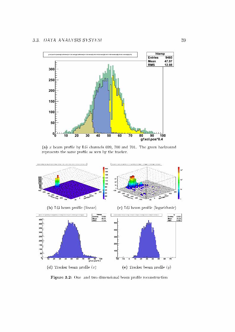
Figure 3.2(a) on page 39 shows our rst attempt, which proceeded as follows:


1. we dened a subset of the data, selecting the entries with χ2 < 10

for every track, in both x and y directions, and low residuals for the

hits positions on the traker chambers (∆x < 10channels and ∆y <

10channels);

2. we plotted the position of the x clusters detected by the rst tracker

chamber (with respect to a system where axes originate at the lower left

corner of the tracker GEM detectors). Since the strip pitch is ∼ 0.4mm,

we compute the position as 0.4 · posCL, where posCL is the position of

the cluster expressed as channel number;

3. we plotted the hits on the LG channels, to nd the most irradiated

ones;

4. we plotted again the distribution of the x clusters detected by the rst

tracker chamber;

5. nally, we selected only the entries containing a hit on one of the most

irradiated LG channels, and we plotted them over the graph produced

at the previous step.

This way we made a sort of puzzle whose pieces represent the beam por-

tion seen by each LG channel. It is like projecting the shadow of the LG pad

corresponding to that channel on the reconstruction of the beam prole by

the tracker.

Figure 3.2(a) on the next page shows that the adopted LG mapping is

correct. Indeed the superposition of signals seen by its pads traces fairly well

out the beam prole drawn by the tracker. The dierent height of the two

proles (the one from the tracker and the one from the LG) is due to the

fact that we did not include some of the adjacent LG channels in the plot,

which indeed caught a little part of the beam.

A two-dimensional plot can be done as well. A GetX() and a GetY()

functions were dened to extract x and y pad position information given the

number of the corresponding channel. Figure 3.2 on the facing page shows

the two-dimensional distribution of the hits detected by the prototype, in


(a) x beam prole by LG channels 699, 700 and 701. The green backroundrepresents the same prole as seen by the tracker.

(b) LG beam prole (linear) (c) LG beam prole (logarithmic)

(d) Tracker beam prole (x) (e) Tracker beam prole (y)

Figure 3.2: One- and two-dimensional beam prole reconstruction


linear (3.2(b)) and logarithmic (3.2(c)) scales, as well as the tracker proles

for comparison (3.2(d) and 3.2(e)).

The beam shown in Figure 3.2 on the previous page is a muon beam,

and thus it is quite large in both directions. Pion beams were more tightly

focused, and almost all the charge was concentrated on no more than four

adjacent pads.

The beam prole reconstruction algorithm proved to work well, and so

did the track reconstruction one.

Figure 3.2(c) on the preceding page gives an idea of the noise aecting

the prototype: some channels are hit even though the beam is focused on

another area. However, the scale of the plot is logarithmic, and in this case

the noise intensity is really negligible with respect of the intensity of the

beam.

Chapter 4On-beam tests

During the test beam we worked at gain values higher than those S. D. Pinto

found, presented in Chapter 1.3.1 on page 22. Table 4.1 on the following

page shows the extrapolated gain values for our working points (with Ar/CO2

70/30), using Pinto's exponential t of his X-Rays gain curve:

G = 2 · 10−6 e0.026·I

The expected current values refer to both the detector sides; actually,

the two sides presented slightly dierent amperage due to small dierences

between the two divider circuits, in the range of Ileft = (Iright + ξ)µA, where

0 ≤ ξ ≤ 4.3.

The gas mixture inside the detector was Ar/CO2 in 70/30 proportions,

where not specied otherwise.

4.1 Eciency of the tracker

When we started using the test beam, we performed an high voltage scan

in order to nd the tracker chambers working point. At rst we computed

its eciency without checking whether the clusters corresponded to actual

41

42 CHAPTER 4. ON-BEAM TESTS

Divider HV (V ) Expected I (µA) Expected Gain

−4, 600 −764.8 1, 930−4, 700 −781.5 3, 021−4, 800 −798.2 4, 767−4, 900 −815.1 7, 403−5, 000 −831.3 11, 684−5, 050 −840.1 15, 100−5, 100 −847.9 18, 439−5, 150 −856.7 22, 947−5, 200 −865.1 29, 737−5, 250 −873.4 37, 206−5, 300 −881.4 45, 599−5, 350 −890.2 57, 104

Table 4.1: Extrapolated gain values for I > 750µA, using Ar/CO2 70/30

tracks, since we already knew from previous tests that the tracker was reli-

able.

We veried the relationships between eciency and threshold, and be-

tween the average size of hit clusters and the threshold; these measurements

were carried out after nding the right latency. Figure 4.1 on the next page

shows the results.

4.2 High voltage scan

The prototype eciency was rst computed as a function of the High-Voltage

(subsequently referred to as HV) applied to the divider poles. These scans

were performed focussing the muon beam on two regions of the chamber (P

and A, whose readout plane areas are covered respectively with large and

small pads). We did it in order to check the behaviour of our detector with

VFAT2 front-ends in the two extreme pad sizes. Slightly dierent results

were obtained.

4.2. HIGH VOLTAGE SCAN 43

(a) Eciency VS threshold (b) Cluster size VS threshold

(c) Eciency VS latency

Figure 4.1: Preliminary tracker tests


Divider HV [kV]4.6 4.7 4.8 4.9 5 5.1 5.2

LG

eff

icie

ncy

0.0

0.1

0.2

0.3

0.4

0.5

0.6

0.7

0.8

0.9

1.0

High Voltage scan (point A)

th -100 DAC steps | MSPL 4clk








Divider current [uA]770 780 790 800 810 820 830 840 850 860 870

(a) Zone A: beam on small pads

Divider HV [kV]4.6 4.7 4.8 4.9 5 5.1 5.2

LG

eff

icie

ncy

0.0

0.1

0.2

0.3

0.4

0.5

0.6

0.7

0.8

0.9

1.0

High Voltage scan (point P)

Threshold -100 DAC steps




Divider current [uA]770 780 790 800 810 820 830 840 850 860 870

(b) Zone P : beam on large pads (MSPL = 4clk)

Figure 4.2: High voltage scans performed with a muon beam focussed on zones A and P

4.2. HIGH VOLTAGE SCAN 45

Four dierent thresholds were applied, in order to have a complete set of

data to be used as reference for future comparison: −40 DAC steps (subse-

quently called ds), −60ds, −80ds and −100ds. The lenght of the monostable

pulse (subsequently referred to as MSPL) was set at 4 clock cycles (clk); in

point A we also repeated the scan with MSPL = 3clk.

Figure 4.2(a) on the facing page shows the results of the HV scan per-

formed when the beam was centered on A, while Figure 4.2(b) shows the

results for P.

The two gures show a higher eciency at lower HV values on the region

made of smaller pads. At rst we supposed that this eect might be due to

the capacitance of the pads themselves, which aects the signal where the

pads are large. We studied this phenomenon, but the results (presented in

Chapter 5.1.2 on page 63) demonstrated that there should be another reason

for this eciency gap.

In zone A we reached about 95% or higher eciency (ε) at thresh-

olds −40ds and −60ds, already with a divider current ID = 817µA. At

ID = 850µA we got ε ' 98% for all the four threshold values. MSPL = 3clk

graphs do not diverge signicantly from MSPL = 4clk ones. Instead, in

zone P the LG prototype approached full eciency for all thresholds only

at ID ≥ 866µA, with ε > 95% at ID = 850µA only for th = −40ds and

th = −60ds data sets.

We also ran an HV scan after changing the gas mixture inside the detector,

as described in Chapter 4.4 on page 51. We added tetrauoromethane (CF4),

obtaining a lower gain. Figure 4.3 on the next page shows a comparison of

the prototype eciency with its standard gas mixture (Ar/CO2 70/30) and

with CF4 (Ar/CO2/CF4 60/20/20). I will come back on the purpose of this

scan in Chapter 4.4 on page 51. The loss of eciency at lower current levels

may be reduced by optimizing the divider in order to make the detector work

with CF4 with appropriate internal electric elds.


Divider HV [kV]4.6 4.7 4.8 4.9 5.0 5.1 5.2 5.3

LG

eff

icie

ncy

0.0

0.1

0.2

0.3

0.4

0.5

0.6

0.7

0.8

0.9

1.0

Gas Mixture comparison

Ar-CO2 70/30

Ar-CO2-CF4 60/20/20

Divider current [uA]770 780 790 800 810 820 830 840 850 860 870 880

Figure 4.3: High voltage scan performed using an Ar/CO2/CF4 60/20/20 gas mixture(same internal voltages and elds as for Ar/CO2)

4.3 Threshold scan

We ran an eciency scan as a function of the VFAT2 threshold level for two

dierent regions of the chamber (A and P). This is particularly useful to

understand how much the threshold can be raised (for example, in order to

work in noisy environments) while avoiding a signicant loss of eciency. To

make the test simpler, we set the same threshold for all the channels at a

time, even if their noise levels were quite dierent. However, a channel by

channel adjustment is available, if needed, through VFAT2 TrimDAC fea-

ture.

Figure 4.4 on the next page shows the results of the test. The response

of the chamber is satisfying: when working at high gain (referring to the

sets of data taken at divider current I ≥ 850µA) we can arbitrarily raise

the threshold to th = 90ds without virtually experiencing any eciency loss.

However, zone P looks again less ecient than zone A.

4.3. THRESHOLD SCAN 47

Negative threshold [VFAT2 DAC steps = 3.3mV = 0.045fC]20 40 60 80 100 120 140 160 180 200 220 240

LG

eff

icie

ncy

0.0

0.1

0.2

0.3

0.4

0.5

0.6

0.7

0.8

0.9

1.0

[MSPL 4clk, lat 14clk]Threshold scan (point A)

A)µHV -5.15kV (859

A)µHV -5.10kV (851

A)µHV -5.05kV (841

A)µHV -5.00kV (834

(a) Point A


LG

eff

icie

ncy

0.60

0.65

0.70

0.75

0.80

0.85

0.90

0.95

1.00

[MSPL 4clk, lat 14clk]Threshold scan (point A)

A)µHV -5.15kV (859

A)µHV -5.10kV (851

A)µHV -5.05kV (841

A)µHV -5.00kV (834

(b) Point A (zoom)


LG

eff

icie

ncy

0.0

0.1

0.2

0.3

0.4

0.5

0.6

0.7

0.8

0.9

1.0

[MSPL 4clk, lat 14clk]Threshold scan (point P)

HV -5.15kV (859uA)

HV -5.10kV (851uA)

HV -5.05kV (841uA)

HV -5.00kV (834uA)

(c) Point P


LG

eff

icie

ncy

0.60

0.65

0.70

0.75

0.80

0.85

0.90

0.95

1.00

[MSPL 4clk, lat 14clk]Threshold scan (point P)

HV -5.15kV (859uA)

HV -5.10kV (851uA)

HV -5.05kV (841uA)

HV -5.00kV (834uA)

(d) Point P (zoom)

Figure 4.4: Threshold scan results for zone A and zone P


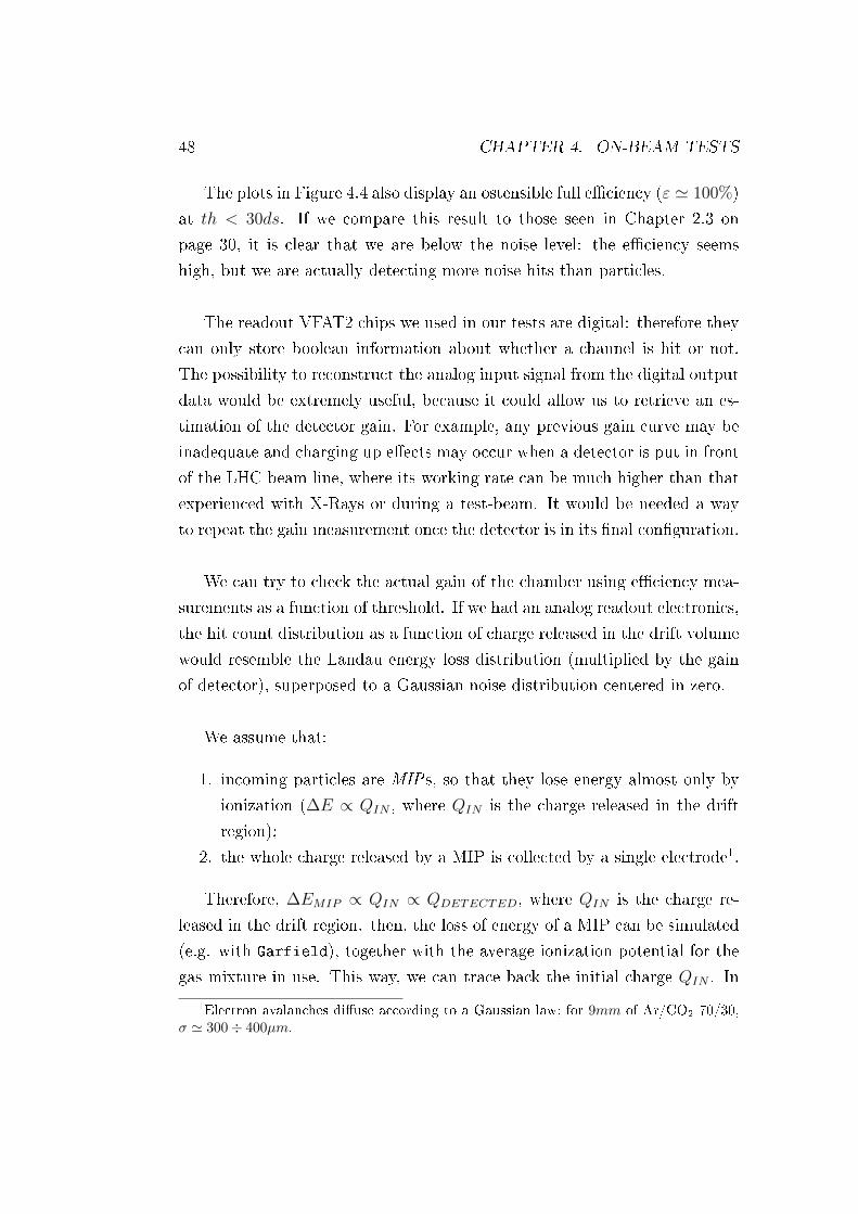
The plots in Figure 4.4 also display an ostensible full eciency (ε ' 100%)

at th < 30ds. If we compare this result to those seen in Chapter 2.3 on

page 30, it is clear that we are below the noise level: the eciency seems

high, but we are actually detecting more noise hits than particles.

The readout VFAT2 chips we used in our tests are digital: therefore they

can only store boolean information about whether a channel is hit or not.

The possibility to reconstruct the analog input signal from the digital output

data would be extremely useful, because it could allow us to retrieve an es-

timation of the detector gain. For example, any previous gain curve may be

inadequate and charging up eects may occur when a detector is put in front

of the LHC beam line, where its working rate can be much higher than that

experienced with X-Rays or during a test-beam. It would be needed a way

to repeat the gain measurement once the detector is in its nal conguration.

We can try to check the actual gain of the chamber using eciency mea-

surements as a function of threshold. If we had an analog readout electronics,

the hit count distribution as a function of charge released in the drift volume

would resemble the Landau energy loss distribution (multiplied by the gain

of detector), superposed to a Gaussian noise distribution centered in zero.

We assume that:

1. incoming particles are MIPs, so that they lose energy almost only by

ionization (∆E ∝ QIN , where QIN is the charge released in the drift

region);

2. the whole charge released by a MIP is collected by a single electrode1.

Therefore, ∆EMIP ∝ QIN ∝ QDETECTED, where QIN is the charge re-

leased in the drift region. then, the loss of energy of a MIP can be simulated

(e.g. with Garfield), together with the average ionization potential for the

gas mixture in use. This way, we can trace back the initial charge QIN . In

1Electron avalanches diuse according to a Gaussian law; for 9mm of Ar/CO2 70/30,σ ' 300÷ 400µm.

4.3. THRESHOLD SCAN 49

3mm of Ar/CO2 70/30 we have QIN ' 28 e−.

The energy loss distribution, when few interactions cause the whole ∆E,

is given by:

f (λ) =1√2π

e−12(λ+e−λ) , λ =

∆E −∆EMP

K ZA

ρβ2X

where ∆EMP is the most probable energy loss (the peak of the Landau dis-

tribution, see for example Figure 4.5 on the next page) and λ represents the

normalized deviation from ∆EMP [14].

We can now t the eciency versus threshold histogram we obtained,

using the reverse integral of the simulated Landau distribution:

F (VTH) = G ·∫ ∞VTH

f (λ) dλ

We use G, the gain of the chamber, as a parameter to be found minimizing

the χ2.

By minimizing the χ2, we can also x another interesting parameter:

the number ne− of electrons whose total charge equals the amplitude of

a threshold bin. Given this value, the conversion from VFAT2 DAC step

bins to charge, expressed as number of electrons, is allowed. We found

that 550 ≤ ne− ≤ 1050 produces a coherent t, which is indeed reason-

able: in principle, for fast signals such as those of GEM detectors, it should

be ∆QBIN ' 0, 045fC ' 280 e−, which is of the same order of magnitude.

Figure 4.6 on the following page shows the results of this study. The

Landau integral t covers only a subset of threshold values: an upper bound

is needed since the ADC may lose linearity above nMAXsteps − 10% ' 230ds2,

while a lower bound allows us to cut the noise Gaussian out of the set of data

2nMAXsteps = 256


Figure 4.5: Simulation of MIPs energy loss distribution in the detector (Gareld)

Threshold [VFAT2 DAC step Bin]0 50 100 150 200 250

Effi

cien

cy

0.70

0.75

0.80

0.85

0.90

0.95

1.00

/ ndf 2χ 1.668 / 9Prob 0.9957p0 0.00215± 0.9902 p1 0± 1050 p2 2274± 3.998e+04 p3 0± 120

/ ndf 2χ 1.668 / 9Prob 0.9957p0 0.00215± 0.9902 p1 0± 1050 p2 2274± 3.998e+04 p3 0± 120

Efficiency vs Threshold

/ ndf 2χ 4.742 / 9Prob 0.8562p0 0.002489± 0.9908 p1 0± 1050 p2 1228± 3.386e+04 p3 0± 120

/ ndf 2χ 4.742 / 9Prob 0.8562p0 0.002489± 0.9908 p1 0± 1050 p2 1228± 3.386e+04 p3 0± 120

/ ndf 2χ 4.742 / 9Prob 0.8562p0 0.002489± 0.9908 p1 0± 1050 p2 1228± 3.386e+04 p3 0± 120

/ ndf 2χ 2.119 / 9

Prob 0.9894p0 0.003086± 0.995 p1 0± 1050 p2 716.7± 2.826e+04 p3 0± 120

/ ndf 2χ 2.119 / 9

Prob 0.9894p0 0.003086± 0.995 p1 0± 1050 p2 716.7± 2.826e+04 p3 0± 120

/ ndf 2χ 2.119 / 9

Prob 0.9894p0 0.003086± 0.995 p1 0± 1050 p2 716.7± 2.826e+04 p3 0± 120

/ ndf 2χ 2.945 / 9

Prob 0.9664p0 0.003474± 0.9987 p1 0± 1050 p2 573.3± 2.579e+04 p3 0± 120

/ ndf 2χ 2.945 / 9

Prob 0.9664p0 0.003474± 0.9987 p1 0± 1050 p2 573.3± 2.579e+04 p3 0± 120

/ ndf 2χ 2.945 / 9

Prob 0.9664p0 0.003474± 0.9987 p1 0± 1050 p2 573.3± 2.579e+04 p3 0± 120

HV = -5.15 kV

HV = -5.10 kV

HV = -5.05 kV

HV = -5.00 kV

Figure 4.6: Eciency versus threshold scan tted by the integral of a Landau energyloss distribution

4.4. TIMING SCAN 51

to be tted. The lower threshold bound was set at −50ds, which was found

to be enough to exclude the noise.

This was a very preliminary analysis, which should be rened in order to

prove the validity of this method, aimed at checking the gain of proportional

chambers in their nal setup and at reconstructing analog inputs from digital

data.

4.4 Timing scan

We worked on some time-performance scans as well, to check how fast the

prototype response was, and what could be done to improve it. First we

estimated the latency via the LabVIEW software that we used to interact

with the VFAT2 chips, and we found it to be around 17 clock cycles. Then

we investigated all the latencies in the [10clk, 19clk] interval by means of a

set of acquisitions at dierent thresholds and MSP lengths.

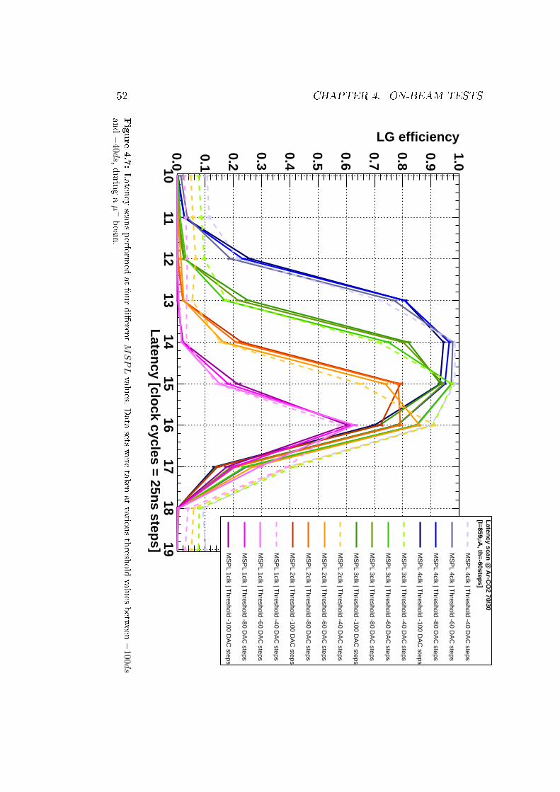
Figure 4.7 on the next page shows all the data sets. Eciency is plotted

versus latency; indeed, the signal starts at 17clk, and the eciency reaches

90% only at low thresholds or atMSPL ≥ 3clk. This is due to the threshold-

crossing time spread, that is longer than a single clock cycle when the detector

is lled with Ar/CO2 (it can reach ∼ 60ns, as pointed out in Chapter 2.1 on

page 29, while a clock cycle lasts 25ns).

We can select two ecient working points:

1. MSPL = 4clk, with any threshold value such that 40ds < th < 100ds;

2. MSPL = 3clk, with threshold 40ds ≤ th ≤ 60ds.

During these tests, the rate of incoming particles was of the order of mag-

nitude of kHz. In LHC, where the rate is much higher, a monostable pulse

lenght > 1clk may cause superposition of events and loss of time resolution.

In that case, we would want to stretch the MSPL as little as possible.


Laten

cy [clock cycles = 25n

s steps]

1011

1213

1415

1617

1819

LG efficiency

0.0

0.1

0.2

0.3

0.4

0.5

0.6

0.7

0.8

0.9

1.0

A, th

=-60steps]

µ[I=859L

atency scan

@ A

r-CO

2 70/30

MS

PL 4clk | T

hreshold -40 DA

C steps

MS

PL 4clk | T

hreshold -60 DA

C steps

MS

PL 4clk | T

hreshold -80 DA

C steps

MS

PL 4clk | T

hreshold -100 DA

C steps

MS

PL 3clk | T

hreshold -40 DA

C steps

MS

PL 3clk | T

hreshold -60 DA

C steps

MS

PL 3clk | T

hreshold -80 DA

C steps

MS

PL 3clk | T

hreshold -100 DA

C steps

MS

PL 2clk | T

hreshold -40 DA

C steps

MS

PL 2clk | T

hreshold -60 DA

C steps

MS

PL 2clk | T

hreshold -80 DA

C steps

MS

PL 2clk | T

hreshold -100 DA

C steps

MS

PL 1clk | T

hreshold -40 DA

C steps

MS

PL 1clk | T

hreshold -60 DA

C steps

MS

PL 1clk | T

hreshold -80 DA

C steps

MS

PL 1clk | T

hreshold -100 DA

C steps

Figure

4.7:Laten

cysca

nsperfo

rmed

atfourdieren

tMSPLvalues.

Data

setswere

taken

atvario

usthresh

old

values

betw

een−100d

sand−40ds,durin

gaµ−beam.

4.4. TIMING SCAN 53

Latency [clock cycles = 25ns steps]10 11 12 13 14 15 16 17 18 19

LG

eff

icie

ncy

0.0

0.1

0.2

0.3

0.4

0.5

0.6

0.7

0.8

0.9

1.0A, th=-60steps]µ[I=859

Latency scan @ Ar-CO2 70/30

MSPL 4clk | Threshold -100 DAC steps








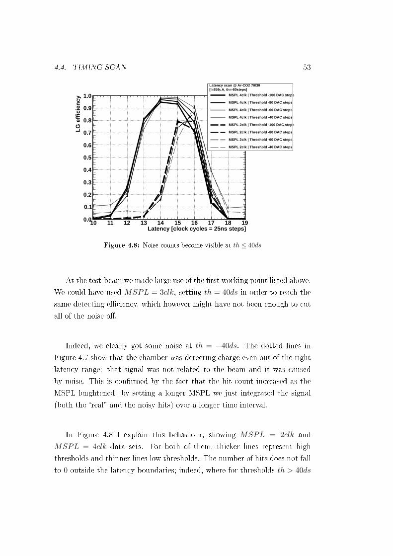
Figure 4.8: Noise counts become visible at th ≤ 40ds

At the test-beam we made large use of the rst working point listed above.

We could have used MSPL = 3clk, setting th = 40ds in order to reach the

same detecting eciency, which however might have not been enough to cut

all of the noise o.

Indeed, we clearly got some noise at th = −40ds. The dotted lines in

Figure 4.7 show that the chamber was detecting charge even out of the right

latency range: that signal was not related to the beam and it was caused

by noise. This is conrmed by the fact that the hit count increased as the

MSPL lenghtened: by setting a longer MSPL we just integrated the signal

(both the real and the noisy hits) over a longer time interval.

In Figure 4.8 I explain this behaviour, showing MSPL = 2clk and

MSPL = 4clk data sets. For both of them, thicker lines represent high

thresholds and thinner lines low thresholds. The number of hits does not fall

to 0 outside the latency boundaries; indeed, where for thresholds th > 40ds


Entries 6389

Mean 0.1473± 383.1

RMS 0.1042± 11.76

Time [ns]320 340 360 380 400 420

Co

un

ts

0

20

40

60

80

100

120

140

160

180

200

220Entries 6389

Mean 0.1473± 383.1

RMS 0.1042± 11.76

TDC_Ch5LargeGEM: TDC MeasurementGas Mixture: Ar/CO2 70/30. H.V.=-5.25kV, 875uA

Pad Type: Larger Size, VFAT2 MSPL=4clk, Threshold=-40 DAC step

Figure 4.9: Distribution of elapsed time between scintillators and VFAT2 S-Bits

the eciencies are null, we see that:

E th=40dsMSPL=4clk ' 2 ∗ E th=40ds

MSPL=2clk (lat ≤ 11clk ∨ lat ≥ 18clk)

With MSPL = 4clk, noise hits are indeed counted for twice as much time

as with MSPL = 2clk.

A histogram3 of the time intervals occurring between the scintillators

trigger and the VFAT2 Fast-OR signal provides further information about

the time resolution of the whole DAQ system4. The narrower this distribution

is, the higher is the time resolution, which indeed is the RMS of the plot in

Figure 4.9.

3Study performed during the previous test beam period (June 2010).4DAQ stands for Data Acquisition. In this case the DAQ system consists of a large

GEM detector with pad readout, and VFAT2 front-end chips.

4.4. TIMING SCAN 55

The same Figure 4.9 also shows that:

< TDC >

1clk (25ns)= ∆t(SCtrigger→FastORtrigger) ' 15clk

which is only relevant if we are unable to set the right DAQ latency, for which

∆t can be used as an upper bound (lat ≤ ∆t).

Increasing detectors time performance is a priority. The LHC machine is

expected to start working at very high frequency and intensity by the end of

2011, with a bunch crossing every 25ns and a luminosity L ≥ 1031 1

cm2 · s.

TOTEM GEM-based detectors (T2) cover a region of very high pseudorapid-

ity5, and therefore they run through extreme radiation conditions. We ran

a test trying to nd a new gas mixture for those TOTEM detectors, which

would allow for a faster detector response without modifying the divider.

A percentage of CF4 was added to the gas mixture inside the LG, getting

to an Ar/CO2/CF4 60/20/20 conguration. After the High-Voltage scan

described in Chapter 4.2 on page 42 we repeated some of the latency scans,

whose results are compared to those we got with the previous gas mixture in

Figure 4.10 on the following page.

We focussed on MSPL = 2clk tests, since a lenght of 2clk would be

suitable for the future TOTEM runs. Figure 4.10(b) on the next page

clearly shows that CF4 improves the response speed of this kind of detec-

tors: the new gas mixture allows to approach full eciency at th = −60ds

and MSPL = 2clk. On the other hand, we needed to supply a little more

current on the divider. We did not observe any discharge, but we could run

only a few tests with this gas mixture. It must be pointed out that we do not

know what the exact gain value of the chamber was when we worked with

CF4. However, previous tests performed by the authors of [7] suggest that

5Being θ the angle between the momentum −→p of the incoming particle and the beam

direction, we dene pseudorapidity η = − ln

(tan

θ

2

). Therefore, as the angle decreases,

η −→∞.



LG

eff

icie

ncy

0.0

0.1

0.2

0.3

0.4

0.5

0.6

0.7

0.8

0.9

1.0A, th=-60steps]µ[I=859

Latency scan @ Ar-CO2 70/30

MSPL 4clk

MSPL 3clk

MSPL 2clk

MSPL 1clk

(a) Standard gas mixture results


LG

eff

icie

ncy

0.0

0.1

0.2

0.3

0.4

0.5

0.6

0.7

0.8

0.9

1.0 [MSPL 2clk, th -60steps]Latency scan

AµI = 859 Ar-CO2 70/30

AµI = 892 Ar-CO2-CF4 60/20/20

(b) Gas mixtures comparison at MSPL =2clk

Figure 4.10: Data taken adding CF4 to the standard Ar/CO2 70/30 gas mixture (sameinternal voltages and elds as for Ar/CO2)

at our working point the gain of Ar/CO2/CF4 60/20/20 mixture was even

lower, by a factor of ve, than that of Ar/CO2 70/30.

The detector was designed to work with Ar/CO2 70/30. It is now clear

that redesigning its divider to work with this new gas mixture should improve

the detector time resolution. In addition, a high eciency should be reached

with a lower gain, which would result in a lower probability of discharge.

4.5 Behaviour with hadron beam

We were given the possibility to test the behaviour of the prototype with

hadron (π−) beams. Particle rates went from 1.25kHz up to 38kHz. Unlike

muon beams, pion beams were sharp: the particle ux covered an area of

approximately 10 · 5mm2.

Figure 4.11(a) on the facing page shows an HV scan performed for dier-

ent intensities of the π− beam. However, for some intensity-threshold com-

binations we only got a few data. The plot shows beam intensities measured

in counts per spill; each spill lasted 10s. Figure 4.12 represents a comparison

between pion beam and muon beam HV scans. It only shows data collected

at threshold −60ds, so to compare two scans with the same settings.

4.5. BEHAVIOUR WITH HADRON BEAM 57

Divider voltage [kV]4.5 4.6 4.7 4.8 4.9 5

LG

eff

icie

ncy

0.0

0.1

0.2

0.3

0.4

0.5

0.6

0.7

0.8

0.9

1.0

Variable intensity hadronsI ~380k c/spill | th -40 DAC steps

I ~380k c/spill | th -60 DAC steps



I ~12.5k c/spill | th -40 DAC steps


(a) HV scan

Divider voltage [kV]4.5 4.6 4.7 4.8 4.9 5

LG

eff

icie

ncy

0.86

0.88

0.90

0.92

0.94

0.96

0.98

1.00

Variable intensity hadronsI ~380k c/spill | th -40 DAC steps






(b) Zoom

Figure 4.11: High-voltage scan under a beam of pions

Divider HV [kV]4.5 4.6 4.7 4.8 4.9 5.0 5.1 5.2

LG

eff

icie

ncy

0.0

0.1

0.2

0.3

0.4

0.5

0.6

0.7

0.8

0.9

1.0

beam comparisonµ - π

beam [~38kHz]π150GeV/c

beam [~0.8kHz]µ150GeV/c

Divider current [uA]750 760 770 780 790 800 810 820 830 840 850 860 870

Figure 4.12: Detector behaviour: comparison between pions exposition and muons ex-position


We may infer from Figure 4.12 that the prototype presents higher ef-

ciency when detecting hadrons. However, due to the large rate dierence

between muon beam (0.8kHz) and hadron beam (Figure 4.12 plots the set of

data collected when the beam intensity was 38kHz), we can not state clearly

whether the increase in eciency is caused by the presence of hadrons. An

eect of charging upmay have indeed occured in this case: as a result of the

higher interaction rate inside the detector, some of the electrons produced in

the avalanche may have accumulated on the insulator surface by the GEM

holes (which are not perfectly straight). As a consequnce, the electric eld in-

side the holes would have been strenghtened, raising the GEM foil gain with

no need of increasing the external voltage. The visible eect of this kind of

charging up should be a raise of eciency at constant divider current, as we

may recognize in Figure 4.12 on the previous page. Figure 4.11(b) on the

preceding page focusses on the slightly dierent behaviours of the detector

when working at dierent rates. To verify this, we shall perform further

laboratory tests, with dierent intensities X-Rays, or maybe organize future

test-beam sessions aimed at solving this question.

Chapter 5Remarks

5.1 (In)homogeneity of the prototype

5.1.1 Critical chamber zones

The availability of such a good tracking system allowed us to highlight some

spatial defects of the prototype. When we direct a ux of charged particles

over a detector, for some reasons the response may vary according to which

region of the chamber is irradiated. For instance, it happened that a pad

was disconnected from the corresponding pin on its VFAT2 chip; or that

we focused the beam over a region of the detector containing a piece of the

spacer frame.

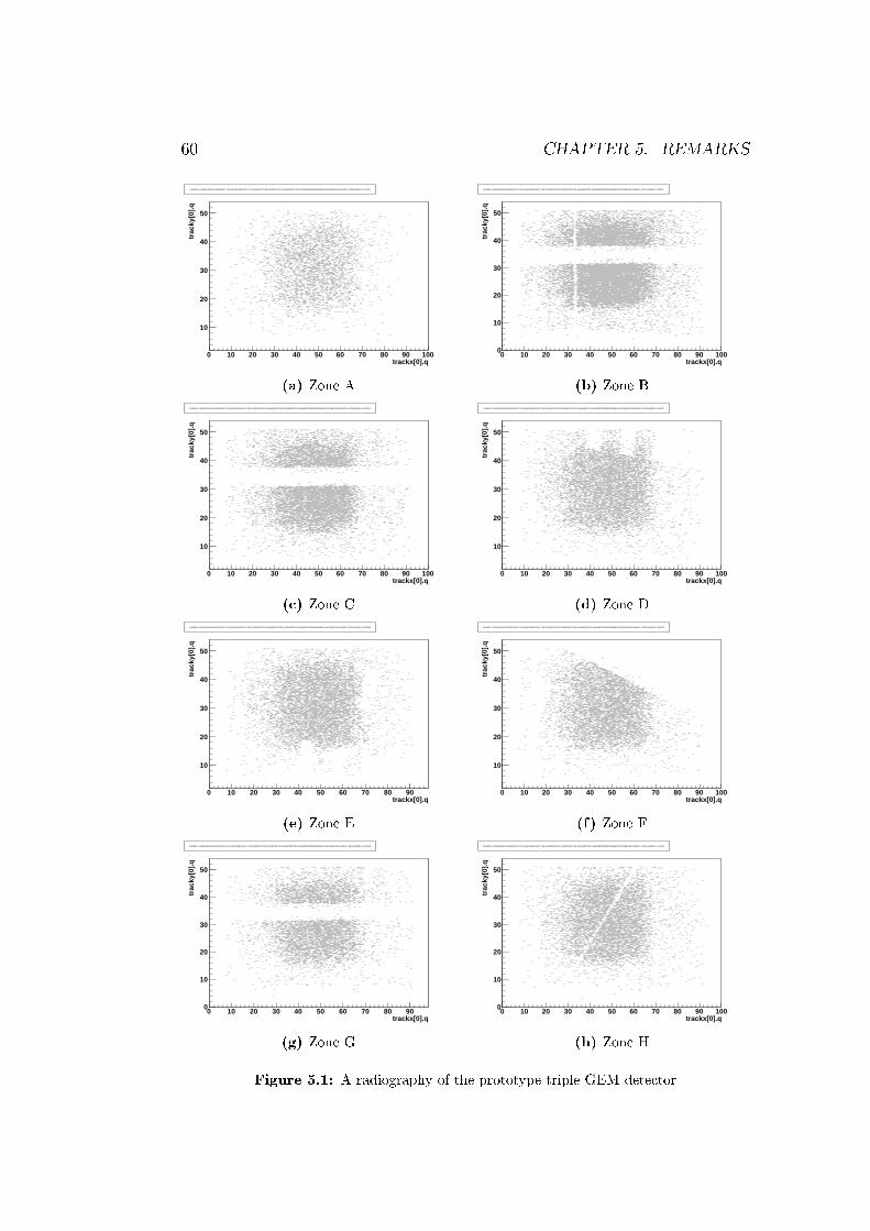
Figures 5.1 on the next page and 5.2 on page 61 display a radiography

of the LG prototype, made by moving the detector around in order to check

the response of several areas (see Figure 1.8(b) on page 21). The graphs

plot the two-dimensional beam prole as it was detected by the tracker, with

the condition that for every track there were corresponding hits on the LG

channels.

We spotted:

• dead (disconnected) pads: see Figures 5.1(d), 5.1(e) and 5.2(c);

59

60 CHAPTER 5. REMARKS

trackx[0].q0 10 20 30 40 50 60 70 80 90 100

trac

ky[0

].q

10

20

30

40

50

tracky[0].q : trackx[0].q ([email protected]()==1 && [email protected]()==1 && trackx[0].chi2<10 && tracky[0].chi2<10 && residualx[0]<10 && residualy[0]<10)&&(dist(GetX(bgch.ch),GetY(bgch.ch),trackx[0]->q - 240.8,tracky[0]->q + 6.3)<6)

(a) Zone A

trackx[0].q0 10 20 30 40 50 60 70 80 90 100

trac

ky[0

].q

0

10

20

30

40

50

tracky[0].q : trackx[0].q ([email protected]()==1 && [email protected]()==1 && trackx[0].chi2<10 && tracky[0].chi2<10 && residualx[0]<10 && residualy[0]<10)&&(dist(GetX(bgch.ch),GetY(bgch.ch),trackx[0]->q - 303.2,tracky[0]->q - 34.4)<7)

(b) Zone B

trackx[0].q0 10 20 30 40 50 60 70 80 90 100

trac

ky[0

].q

10

20

30

40

50

tracky[0].q : trackx[0].q ([email protected]()==1 && [email protected]()==1 && trackx[0].chi2<10 && tracky[0].chi2<10 && residualx[0]<10 && residualy[0]<10)&&(dist(GetX(bgch.ch),GetY(bgch.ch),trackx[0]->q - 362.9,tracky[0]->q - 34)<8.5)

(c) Zone C

trackx[0].q0 10 20 30 40 50 60 70 80 90 100

trac

ky[0

].q

10

20

30

40

50


(d) Zone D

trackx[0].q0 10 20 30 40 50 60 70 80 90

trac

ky[0

].q

10

20

30

40

50


(e) Zone E

trackx[0].q0 10 20 30 40 50 60 70 80 90 100

trac

ky[0

].q

10

20

30

40

50


(f) Zone F

trackx[0].q0 10 20 30 40 50 60 70 80 90

trac

ky[0

].q

0

10

20

30

40

50

tracky[0].q : trackx[0].q ([email protected]()==1 && [email protected]()==1 && trackx[0].chi2<10 && tracky[0].chi2<10 && residualx[0]<10 && residualy[0]<10)&&(dist(GetX(bgch.ch),GetY(bgch.ch),trackx[0]->q - 482.6,tracky[0]->q - 34.1)<12)

(g) Zone G

trackx[0].q0 10 20 30 40 50 60 70 80 90 100

trac

ky[0

].q

0

10

20

30

40

50


(h) Zone H

Figure 5.1: A radiography of the prototype triple GEM detector

5.1. (IN)HOMOGENEITY OF THE PROTOTYPE 61

trackx[0].q0 10 20 30 40 50 60 70 80 90 100

trac

ky[0

].q

0

10

20

30

40

50


(a) Zone I

trackx[0].q0 10 20 30 40 50 60 70 80 90 100

trac

ky[0

].q

10

20

30

40

50

tracky[0].q : trackx[0].q ([email protected]()==1 && [email protected]()==1 && trackx[0].chi2<10 && tracky[0].chi2<10 && residualx[0]<10 && residualy[0]<10)&&(dist(GetX(bgch.ch),GetY(bgch.ch),trackx[0]->q - 663.4,tracky[0]->q - 1.1)<23.5)

(b) Zone L

trackx[0].q0 10 20 30 40 50 60 70 80 90 100

trac

ky[0

].q

10

20

30

40

50

tracky[0].q : trackx[0].q ([email protected]()==1 && [email protected]()==1 && trackx[0].chi2<10 && tracky[0].chi2<10 && residualx[0]<10 && residualy[0]<10)&&(dist(GetX(bgch.ch),GetY(bgch.ch),trackx[0]->q - 664.9,tracky[0]->q + 108)<30)

(c) Zone M

trackx[0].q0 10 20 30 40 50 60 70 80 90

trac

ky[0

].q

10

20

30

40

50


(d) Zone N

trackx[0].q0 10 20 30 40 50 60 70 80 90 100

trac

ky[0

].q

10

20

30

40

50


(e) Zone O

trackx[0].q0 10 20 30 40 50 60 70 80 90 100

trac

ky[0

].q

0

10

20

30

40

50


(f) Zone P

Figure 5.2: A radiography of the prototype triple GEM detector


Chamber zones (from A to P)

LG

eff

icie

ncy

(%

)

0

10

20

30

40

50

60

70

80

90

100

Homogeneity scan

(a) LG eciency (b) Spacer frame view

Figure 5.3: Eciency scan over various critical chamber regions. On the right, a brokenGEM layer and its spacer frame (same model as those inserted in the prototype undertest)

• thin spacers: see Figures 5.1(b), 5.1(h), 5.2(b), 5.2(c), 5.2(d) and 5.2(f).

In particular, Figure 5.2(c) shows a misalignment between a spacer and

the edge of a cathode sector;

• segments of the thick central spacer covering the seam between the

GEM foils: see Figures 5.1(b), 5.1(c) and 5.1(g);

• the edge of the chamber: see Figures 5.1(f) and 5.2(d).

Figure 5.3(a) and Table 5.1 on page 69 show the computed average e-

ciency for all these regions, and some more information that will be discussed

below.

A deeper study of the response of the detector in the junction area (Fig-

ure 5.4(a) on the facing page) shows the steepness of the slope in the curve

of eciency as a function of y, which in that plot varies perpendicularly to

the spacer that covers the seam. We can see that the low-eciency area

around the spacer is narrow, as required. No collateral malfunctionings were

observed in spacer, border and junction areas.

However, Figure 5.4(a) on the next page also shows an unexpected prob-

lem, which we became aware of only long after the end of the test beam: the


Y [mm]15 20 25 30 35 40 45

LG

eff

icie

ncy

0.0

0.1

0.2

0.3

0.4

0.5

0.6

0.7

0.8

0.9

1.0

LG efficiency over GEM foils junction - point C

(a) Eciency versus y (b) Spacer and inactivearea width

Figure 5.4: Loss of eciency at the GEM foils junction

side of the detector which was not directly involved in the tests appears to

be less ecient. This eect may be too high to be explained in terms of lack

of charging-up, and it is visible in all the three junction zones we analized.

It is not due to visible asymmetries between the two voltage distribution

boards either, whose input impedances were both measured to be equal to

5.40MΩ. The set of data we gathered so far is not enough to allow a proper

explanation of this phenomenon.

As already said, we came across this problem after the test beam period

nished, and thus we were not able to set up another irradiation test to

investigate it. A new gain curve is needed and will be worked out as soon as

possible with Cu X-Rays, to compare it with the absolute gain calibration

made by S. D. Pinto [13].

5.1.2 Eects of the dierent pad dimensions

It is expected that larger copper pads have bigger capacitance. Comparing

the two Figures 4.2(a) and 4.2(b) on page 44, we may conjecture that the

loss of eciency in zone P is due to the bigger pads capacitance, which could

cause noise and channel coupling.


Figure 5.5: How a calibration pulse scan works

Being noise proportional to the electrode capacitance [6], we decided to

run a noise measurement for each channel. This way we could collect infor-

mation about the capacitance of each readout pad.

An o-beam analysis was thus performed, injecting calibration charge

pulses of increasing amplitude to all of the pads via the VFAT2 chips, and

tting the S-Curves of each channel with an erf function.

The erf function, also known as Gaussian error function, is dened

as:

erf(x) =2√π

∫ x

0

e−t2

dt

After we dene a threshold for the VFAT2 chips, and we start injecting

charge, as long as the injected potential (Q = CV ) is under threshold

(∆V < th) the output of the comparator is low. Then, like an heaviside

step function, it should go high as soon as the pulse amplitude overcomes

the threshold. Actually, if we take the contribution of the noise to the shapes

of the calibration pulses into account (see Figure 5.5), we can only predict


VCal [VFAT2 DAC step Bins]40 60 80 100 120 140 160 180 200

Co

un

ts

0

0.1

0.2

0.3

0.4

0.5

0.6

0.7

0.8

0.9

1

VFAT3 S-Curve

(a) S-Curve

Pad distance from chamber's vertex [mm]200 300 400 500 600 700

No

ise

amp

litu

de

[VFA

T2

DA

C s

tep

s]

2

4

6

8

10

12

14

16

18

20S-Curve sigma distribution

VFAT0VFAT1VFAT2VFAT3VFAT4VFAT5VFAT6

(b) S-Curve sigma vs pad largeness

Figure 5.6: An S-Curve tted by an erf function. On the right, the standard deviation(sigma) of the pad's S-Curve is plotted as a function of the radial position of the pad inthe detector, and thus as a function of its increasing largeness.

that the output of the comparator goes high at a certain input charge value

with a Gaussian probability, centered around the given threshold value.

An S-Curve is a histogram of hits for a given threshold, counted while

varying the injected charge [5]; it corresponds to the shape of the erf func-

tion. Indeed, the same plot can be obtained by integrating the Gaussian

distribution of the noise for any VFAT2 channel. Once an S-Curve is tted

with an erf function, the noise distribution sigma is the same as that of the

erf function, and the mean value corresponds to the threshold potential1.

Figure 5.6(b) allows us to state that the lack of eciency of zone P is

not caused by parasitic capacitance of its pads: the larger pads (those at the

right side of the plot) do not show a signicant increase of noise.

According to VFAT2 specications in [6], each channel should have

QEQnoise = 400e− + 50

e−

pF

1ROOT stores the t functions as objects, and makes their parameters (mean, RMS,sigma, and so on) available via calls to the objects themselves. To compute the sigmas ofFigure 5.6(b), we tted the S-Curve of each channel with erf functions and plotted theirsigma parameters.


where QEQnoise is the equivalent charge due to the noise, and the picofarads

refer to the channel input capacitance. Assuming 300 ÷ 400 electrons per

VFAT2 DAC step bin, with an S-Curve sigma σ ' 7 for all channels we can

estimate an average input capacitance of about 48pF .

Another reason for the dierence in response between point P and point

A is to be found. More tests will be performed as soon as possible.

5.2 Eciency radius lenght: noise checks

In Chapter 3.3.1 on page 35 I explained how we compute eciency. If a hit

occurs in the Large GEM within a given radius (eciency radius) from the

projection of the track of the particle, then we say that the chamber has been

ecient. If there are no hits within the eciency radius, the chamber has

been inecient.

What happens if we set a wrong eciency radius? There are two scenar-

ios:

1. the radius is too short. In a large-pads area we may not include a whole

pad within the radius, and the eciency-computing algorithm might

miss some hits.

2. the radius is too long. Some noise hits on adjacent pads may be mis-

taken as ecient hits.

Figure 5.7 on the next page shows, for every zone we tested, the uctu-

ation of the computed eciency for increasing eciency radius values. It is

clear then that 20mm ≤ effrad ≤ 30mm would be appropriate for every

purpose.

Actually, all the results discussed here were computed trying to minimize

the eciency radius for each zone of the chamber, in order to include as few

noise hits as possible. For each zone, the eciency radius was set to the

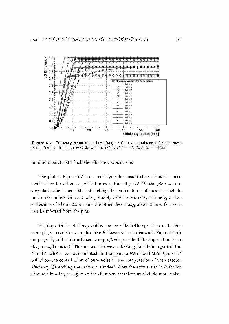
5.2. EFFICIENCY RADIUS LENGHT: NOISE CHECKS 67

Efficiency radius [mm]0 10 20 30 40 50 60

LG

Eff

icie

ncy

0.0

0.1

0.2

0.3

0.4

0.5

0.6

0.7

0.8

0.9

1.0

LG efficiency versus efficiency radiusPoint APoint BPoint CPoint DPoint EPoint FPoint GPoint HPoint IPoint LPoint MPoint NPoint OPoint P

Figure 5.7: Eciency radius scan: how changing the radius inuences the eciency-computing algorithm. Large GEM working point: HV = −5.15kV , th = −40ds

minimum length at which the eciency stops rising.

The plot of Figure 5.7 is also satisfying because it shows that the noise

level is low for all zones, with the exception of point M : the plateaus are

very at, which means that stretching the radius does not mean to include

much more noise. Zone M was probably close to two noisy channels, one at

a distance of about 20mm and the other, less noisy, about 35mm far, as it

can be inferred from the plot.

Playing with the eciency radius may provide further precise results. For

example, we can take a couple of the HV scan data sets shown in Figure 4.2(a)

on page 44, and arbitrarily set wrong osets (see the following section for a

deeper explanation). This means that we are looking for hits in a part of the

chamber which was not irradiated. In that part, a scan like that of Figure 5.7

will show the contribution of pure noise to the computation of the detector

eciency. Stretching the radius, we indeed allow the software to look for hit

channels in a larger region of the chamber, therefore we include more noise.



LG

Eff

icie

ncy

(w

ron

g o

ffse

ts)

-310

-210

-110

1

Noise contribution

HV -4.60kV; TH -40ds



LG out-beam efficiency versus efficiency radius

(a) Zone A


LG

Eff

icie

ncy

(w

ron

g o

ffse

ts)

-410

-310

-210

Noise contribution




LG out-beam efficiency versus efficiency radius

(b) Zone P

Figure 5.8: O-beam eciency computation: evaluating the contribution of noise

Table 5.1 on the next page shows, for each scanned zone:

• the best eciency radius, according to Figure 5.7;

• the level of eciency of that chamber sector, computed with the chosen

best eciency radius;

• the contribution of noise to the computation of eciency, at the same

eciency radius. The noise values are plotted like in Figure 5.82, which

show the eciency of a non-irradiated sector as a function of the e-

ciency radius.

The errors in the eciency column are statistical:

∆ε =ε(1− ε)√

n

where n is the number of events collected and ε is the computed eciency.

These errors must be added to those of the following column.

Table 5.1 therefore shows how noise must be computed to determine which

errors aect the eciency values. If we made this scan on-beam, these eects

would be negligible, because the charge released by incoming particles would

dominate.2Figure 5.8(a) shows that zone A is close to some noisy channels. Indeed, with an

eciency radius of 60mm the eciency grows to signicant values; however, effrad =6mm excludes virtually all noise from the scans.

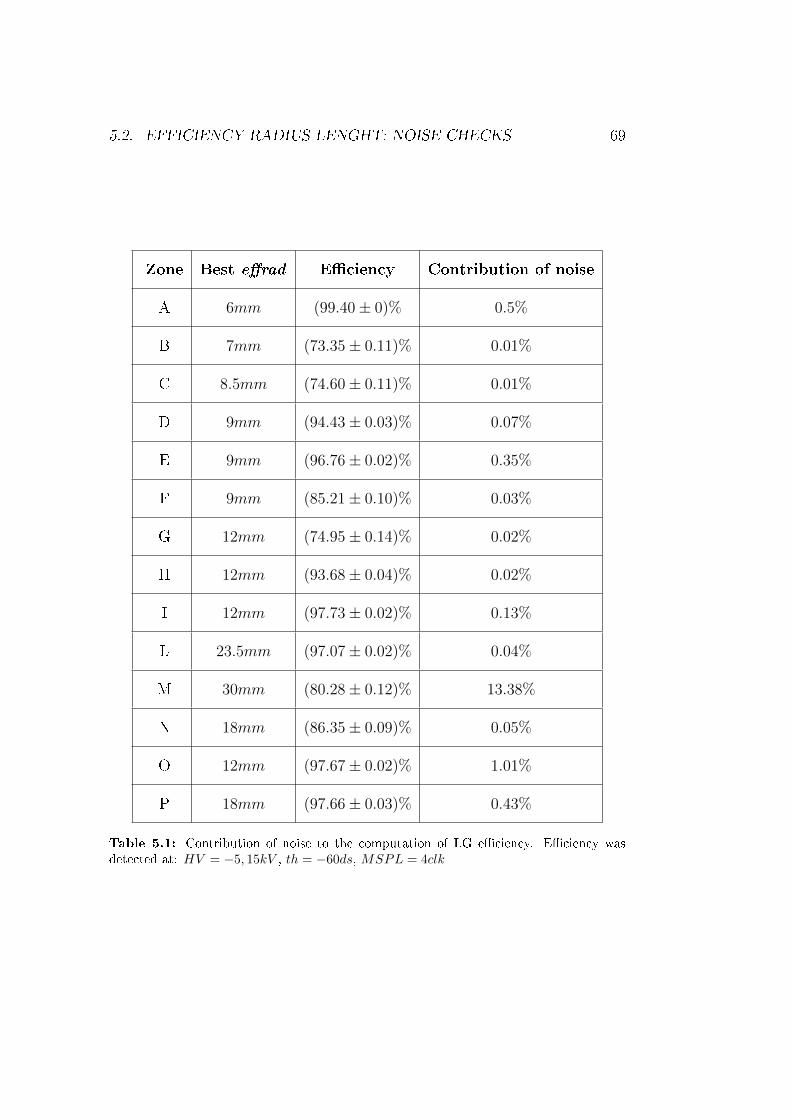
5.2. EFFICIENCY RADIUS LENGHT: NOISE CHECKS 69

Zone Best erad Eciency Contribution of noise

A 6mm (99.40± 0)% 0.5%

B 7mm (73.35± 0.11)% 0.01%

C 8.5mm (74.60± 0.11)% 0.01%

D 9mm (94.43± 0.03)% 0.07%

E 9mm (96.76± 0.02)% 0.35%

F 9mm (85.21± 0.10)% 0.03%

G 12mm (74.95± 0.14)% 0.02%

H 12mm (93.68± 0.04)% 0.02%

I 12mm (97.73± 0.02)% 0.13%

L 23.5mm (97.07± 0.02)% 0.04%

M 30mm (80.28± 0.12)% 13.38%

N 18mm (86.35± 0.09)% 0.05%

O 12mm (97.67± 0.02)% 1.01%

P 18mm (97.66± 0.03)% 0.43%

Table 5.1: Contribution of noise to the computation of LG eciency. Eciency wasdetected at: HV = −5, 15kV , th = −60ds, MSPL = 4clk


5.3 Analysis algorithms: cuts

Chapter 3.3.1 on page 35 points out that tracks are reconstructed only in

some simple cases. In addition, during the analysis process we only used the

tracks satisfying the following conditions:

1. there is exactly one x-track and one y-track per event;

2. χ2 < 10 for both the x-track and the y-track ;

3. the distance between the hits on the tracker chambers and their rst

order polinomial t dening the track is < 10mm for every hit.

Inside a ROOT framework, this means to declare a TCut object that will be

used as a mandatory option while selecting the data to process:

TCut goodtr ( " goodtr " , " trackx@ . GetEntr ies ( )==1 && tracky@ . GetEntr ies ( )==1 && trackx [ 0 ] .

chi2 <10 && tracky [ 0 ] . chi2 <10 && re s i dua l x [0] <10 && re s i dua l y [0] <10" )

Most of the analysis processes exploit the ROOT Draw() command, that

accepts TCut objects as options. For the data sets we have seen so far, whose

acquisition needed the chamber to be shifted 14 times, we had to declare the

(x, y) osets of the chamber with respect to the center of the beam each time.

We achieved that again via TCut objects, which also contained a denition

of eciency radius. The following declarations were used:

TCut Aef f ( "Aef f " , " d i s t (GetX( bgch . ch ) ,GetY( bgch . ch ) , t rackx [0]−>q − 240 .8 , t racky [0]−>q +

6 . 3 )<6" )

TCut Be f f ( " Be f f " , " d i s t (GetX( bgch . ch ) ,GetY( bgch . ch ) , t rackx [0]−>q − 303 .2 , t racky [0]−>q −34 . 4 )<7" )

TCut Cef f ( "Cef f " , " d i s t (GetX( bgch . ch ) ,GetY( bgch . ch ) , t rackx [0]−>q − 362 .9 , t racky [0]−>q −34) <8.5" )

TCut Def f ( "Def f " , " d i s t (GetX( bgch . ch ) ,GetY( bgch . ch ) , t rackx [0]−>q − 362 .9 , t racky [0]−>q +

5 . 6 )<9" )

TCut Ee f f ( " Ee f f " , " d i s t (GetX( bgch . ch ) ,GetY( bgch . ch ) , t rackx [0]−>q − 362 .7 , t racky [0]−>q +

46 .9 )<9" )

TCut Fe f f ( " Fe f f " , " d i s t (GetX( bgch . ch ) ,GetY( bgch . ch ) , t rackx [0]−>q − 362 .8 , t racky [0]−>q +

86 .2 )<9" )

TCut Gef f ( "Gef f " , " d i s t (GetX( bgch . ch ) ,GetY( bgch . ch ) , t rackx [0]−>q − 482 .6 , t racky [0]−>q −34 . 1 )<12" )

TCut Hef f ( "Hef f " , " d i s t (GetX( bgch . ch ) ,GetY( bgch . ch ) , t rackx [0]−>q − 482 .6 , t racky [0]−>q +

6 . 7 )<12" )

TCut I e f f ( " I e f f " , " d i s t (GetX( bgch . ch ) ,GetY( bgch . ch ) , t rackx [0]−>q − 482 .7 , t racky [0]−>q +

86 .3 )<12" )

TCut Le f f ( " Le f f " , " d i s t (GetX( bgch . ch ) ,GetY( bgch . ch ) , t rackx [0]−>q − 663 .4 , t racky [0]−>q −1 . 1 ) <23.5" )

TCut Meff ( "Meff " , " d i s t (GetX( bgch . ch ) ,GetY( bgch . ch ) , trackx [0]−>q − 664 .9 , t racky [0]−>q +

108)<30" )

TCut Nef f ( "Nef f " , " d i s t (GetX( bgch . ch ) ,GetY( bgch . ch ) , t rackx [0]−>q − 662 .5 , t racky [0]−>q +

207 .3 )<18" )

5.3. ANALYSIS ALGORITHMS: CUTS 71

TCut Oef f ( "Oef f " , " d i s t (GetX( bgch . ch ) ,GetY( bgch . ch ) , trackx [0]−>q − 483 .8 , t racky [0]−>q +

46 .7 )<12" )

TCut Pe f f ( " Pe f f " , " d i s t (GetX( bgch . ch ) ,GetY( bgch . ch ) , t rackx [0]−>q − 695 .2 , t racky [0]−>q +

49 .3 )<18" )

where the rst two numbers in each string represent the (x, y) position of the

chamber for the specic data set, and the last one is the best tting eciency

radius.

This approach worked ne. The software did not run across any problems

when variables were declared this way, and selecting tracks according to strict

rules did not aect the analysis process, as the amount of data acquired

during the test-beam period was huge.

Chapter 6Conclusions

6.1 Quality of the large GEM prototype

The performances of the detector were within the expectations. We did not

encounter any problems during the test beam DAQ sessions: the prototype

resisted and detected both muon and pion beams of various intensities.

As expected, the use of CF4 improves the time response of the detector,

even if its elds and internal structure1 are left unchanged. In order to get

even better performances, a revision is needed of the detector design (includ-

ing its high voltage divider). This might be achieved by joining our eorts

with the CMS experiment and the group of A. Sharma, whose recent studies

were in the same direction as ours.

According to the manufacturers, the diculties encountered during the

assembly do not justify the advantage of splicing GEM foils together in order

to cover larger areas and thus to reduce the number of detectors. For exam-

ple, there are currently no proper machines for stretching large foils with an

irregular shape.

As we will discuss in Chapter 6.2, we needed to test if the detector, with its

1Most of all, the height of the internal gaps.

73

74 CHAPTER 6. CONCLUSIONS

Figure 6.1: An arrangement to replace the current T1 CSC telescope of TOTEM [12]

large capacitance readout electrodes, could work eciently with the TOTEM

readout system. The initial intense noise was removed by improving the chip

grounding on the detector. Additional VFAT2 features, such as TrimDAC,

may be used in order to improve the global SNR ratio.

As a nal remark, it should be mentioned that these deep investigations

were made possible thanks to the RD51-GDD tracker telescope, which could

largely improve the resolution and comprehension of the data we collected.

6.2 Large GEMs for TOTEM and CMS

The GDD group, and ours, conceived the Large GEM as a replacement for

the current T1 forward telescope of the TOTEM experiment at the LHC,

which is now made of Cathode Strip Chamber detectors. T1 consists of two

arms, each of them precisely tting in a gap around the beam pipe and in-

side the inner surface of the CMS detectors, in symmetric positions around

Interaction Point 5. It covers the pseudorapidity region 3, 1 ≤ |η| ≤ 4, 7.

A renovation is needed for T1, as its CSC chambers may start ageing fast

when the LHC machine will start to run at luminosity L ≥ 1031 1

cm2 · s. In

particular, it is expected that if luminosity overcomes that level by two orders

of magnitude, the CSCs would age in a few months [10]. However, according

6.2. LARGE GEMS FOR TOTEM AND CMS 75

Figure 6.2: Two readout board options for a large triple GEM detector

to informal reports of ongoing T1 data acquisition sessions, discharges are

already being observed at a luminosity L ' 1030 1

cm2 · s.

The same structure can be built with large GEM chambers, arranging

six discs for each arm, where a disc is made of two planes of 5 chambers

in a back-to-back arrangement (Figure 6.1 on the preceding page). Overlap

regions would ensure a 360 coverage and allow to adjust the radius of the

six discs on demand [13].

As an alternative [10], each disc may be made of six detectors on a sin-

gle plane; they could be alternated in back-to-back conguration, each disc

oset by 30 from the adjacent ones, to allow overlay. Four such sets would

be enough to equip an arm of the future T1.

As in Figure 6.2, readout boards would be pad based, like in the proto-

type, featuring 16 · 64 = 1024 pads of various dimensions.

76 CHAPTER 6. CONCLUSIONS

With respect to CSC, GEM chambers oer high rate tolerance, limited

discharge probability (less than 10−12 at gain G ' 104), high time resolution.

For the prototype analized in this thesis, RMS ' 11.8ns (see Figure 4.9 on

page 54), and it may be improved by adding CF4.

In conclusion, T1 had been designed for a bunch crossing rate f ≥ 75ns

and luminosity L ≤ 1031, while in principle a GEM based substitute could

survive for years at L = 1033 and would be suitable for faster bunch crossing

by just adding a percentage of CF4 to the internal gases [10].

The CMS experiment is also developing similar large GEM prototypes,

with a compatible readout, foreseeing a project for muon detecting in the

forward region. 50cm wide GEM foils are being produced with no need for

splicing.

At the same time, the INFN section in Bari is working on LASER ablation

of GEM foils, a technique that could make automation of mass-manufacturing

easier, and possibly increase hole precision and density.

A new generation of GEM detectors has denitely been started. The

large active surface and quite simple readout system of these new detectors

will prove useful to better reveal high energy particles both from accelerators

and cosmic rays. They might also bear signicant improvements in dierent

research elds, such as low-energy or medical physics, and path a way to

possible new applications.

Appendix AROOT analysis routines

Two young researchers1 from RD51 built the low-level macros used to con-

vert the binary output of the detectors to much more physicist-friendly

ROOT n-tuples.

My personal work consisted in writing down some routines in order to

extract eciency values from specic n-tuples, and make the data accessible

via plots. The following pages collect the most signicant pieces of code I

wrote. In order to meet dierent data sets, raw data le names and break

conditions should be modied.

A.1 Data reconstructing algorithms

Listing A.1: Builder.C

#include <st r ing>

#include <iostream>

#include <TTree . h>

#include <TFile . h>

int EventBuilderVFAT( const char∗ rawfi lename ,

const char∗ root f i l ename ,

const int readmaxevent ) ;

using namespace std ;

1Matteo Alfonsi (CERN) and Gabriele Croci (PhD student at the University of Siena)

77

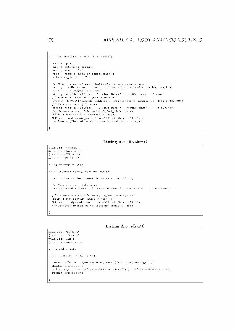
78 APPENDIX A. ROOT ANALYSIS ROUTINES

void Bui lder ( s t r i n g rawf i l e_addres s )

s i ze_t spos ;

s i ze_t substr ing_lenght ;

s t r i n g s l a sh = "/" ;

spos = rawf i l e_addres s . r f i n d ( s l a sh ) ;

substr ing_lenght = 7 ;

// Extracts the s tr ing "Run####" from the rawf i l e name

s t r i n g rawfile_name = rawf i l e_addres s . subs t r ( spos+5, substr ing_lenght ) ;

// Sets the output f i l e name

s t r i n g r o o t f i l e_add r e s s = " . . / RootData/" + rawfile_name + " . root " ;

// Builds a . root f i l e from a rawf i l e

EventBuilderVFAT( rawf i l e_addres s . c_str ( ) , r o o t f i l e_add r e s s . c_str ( ) ,100000000) ;

// Sets the reco f i l e name

s t r i n g r e c o f i l e_add r e s s = " . . / RootData/" + rawfile_name + "_reco . root " ;

// Creates a reco f i l e using Offset_Settings . t x t

TFile f i l e 0 ( r o o t f i l e_add r e s s . c_str ( ) ) ;

TTree∗ t = dynamic_cast<TTree∗>( f i l e 0 . Get ( " rd51tb " ) ) ;

t−>Process ( "Reco2d_ps .C+" , r e c o f i l e_add r e s s . c_str ( ) ) ;

Listing A.2: Recoizer.C

#include <st r ing>

#include <iostream>




void Reco izer ( s t r i n g root f i l e_name )

s t r i n g run_number = rootf i l e_name . subs t r (15 ,4 ) ;

// Sets the reco f i l e name

s t r i n g recof i le_name = " . . / RootData/Run" + run_number + "_reco . root " ;

// Creates a reco f i l e using Offset_Settings . t x t

TFile f i l e 0 ( root f i l e_name . c_str ( ) ) ;


t−>Process ( "Reco2d_ps .C+" , recof i le_name . c_str ( ) ) ;

Listing A.3: eex2.C

#include "TFile . h"

#include "TTree . h"

#include "TH1. h"

#include <iostream>

using std : : cout ;

double e f f e x 2 ( TFile& f i l e 0 )

TH1F∗ he f fbgch = dynamic_cast<TH1F∗>( f i l e 0 . Get ( " he f fbgch " ) ) ;

double e f f i c i e n c y ;

e f f i c i e n c y = 1 − hef fbgch−>GetBinContent (1) / hef fbgch−>GetEntr ies ( ) ;

return e f f i c i e n c y ;

A.1. DATA RECONSTRUCTING ALGORITHMS 79

Listing A.4: eerrors.cc

#include <st r ing>

#include <iostream>

#include <sstream>



#include <cstd io>

#include <TH1. h>

#include <TVectorT . h>


double e f f e x 2 ( TFile& f i l e 0 ) ;

// Gives a fa s t print of e f f i c i ency and

// corresponding s t a t i s t i c a l errors

void e f f e r r o r s ( long int run_number , long int last_run )

Int_t s i z e = last_run − run_number + 1 ;

TVectorD nRun ( s i z e ) ;

TVectorD run_eff ( s i z e ) ;

TVectorD e r r o r s ( s i z e ) ;

Int_t count = 0 ;

long int j = run_number ;

for ( long int i=j ; i<last_run+1; i++)

s t r i n g s ;

char run_n [ 3 ] ;

s p r i n t f ( run_n , "%ld " , i ) ;

s = s t r i n g ( run_n) ;

s t r i n g root f i l e_name = " . . / RootData/Run0" + s + " . root " ;

s t r i n g recof i le_name = " . . / RootData/Run0" + s + "_reco . root " ;

TFile f i l e 0 ( recof i le_name . c_str ( ) ) ;

double e f f = e f f e x 2 ( f i l e 0 ) ;

run_eff [ count ] = e f f ;

nRun [ count ] = i ;

TH1F∗ he f fbgch = dynamic_cast<TH1F∗>( f i l e 0 . Get ( " he f fbgch " ) ) ;

double n = hef fbgch−>GetEntr ies ( ) ;

double s t a t e r r o r = e f f ∗ (1 − e f f ) / sq r t ( n ) ;

e r r o r s [ count ] = s t a t e r r o r ;

count = count + 1 ;

f i l e 0 . Close ( ) ;

Listing A.5: GetOsets.cpp

// Given user−measured o f f s e t s , t h i s

// computes and prints the exact o f f s e t s

// ( the coordinates of the irradiated zones )

TCut goodtr ( " goodtr " , " trackx@ . GetEntr ies ( )==1 && tracky@ . GetEntr ies ( )==1 &&

trackx [ 0 ] . chi2 <10 && tracky [ 0 ] . chi2 <10 && re s i dua l x [0] <10 && re s i dua l y [0] <10" ) ;

// Uncomment the desired zone

// where to compute o f f s e t s

TCut Aef f ( "Aef f " , " d i s t (GetX( bgch . ch ) ,GetY( bgch . ch ) , t rackx [0]−>q − 263 , tracky

[0]−>q + 13 .5 )<30" ) ;

// TCut Beff ("Beff " ," d i s t (GetX(bgch . ch) ,GetY(bgch . ch) , trackx [0]−>q − 323 , tracky

[0]−>q − 26.5)<30") ;

// TCut Ceff ("Ceff " ," d i s t (GetX(bgch . ch) ,GetY(bgch . ch) , trackx [0]−>q − 383 , tracky

[0]−>q − 26.5)<30") ;


// TCut Deff ("Deff " ," d i s t (GetX(bgch . ch) ,GetY(bgch . ch) , trackx [0]−>q − 383 , tracky

[0]−>q + 13.5)<30") ;

// TCut Eeff ("Eeff " ," d i s t (GetX(bgch . ch) ,GetY(bgch . ch) , trackx [0]−>q − 383 , tracky

[0]−>q + 53.5)<30") ;

// TCut Feff (" Feff " ," d i s t (GetX(bgch . ch) ,GetY(bgch . ch) , trackx [0]−>q − 383 , tracky

[0]−>q + 93.5)<30") ;

// TCut Geff ("Geff " ," d i s t (GetX(bgch . ch) ,GetY(bgch . ch) , trackx [0]−>q − 503 , tracky

[0]−>q − 26.5)<30") ;

// TCut Heff ("Heff " ," d i s t (GetX(bgch . ch) ,GetY(bgch . ch) , trackx [0]−>q − 503 , tracky

[0]−>q + 13.5)<30") ;

// TCut I e f f (" I e f f " ," d i s t (GetX(bgch . ch) ,GetY(bgch . ch) , trackx [0]−>q − 503 , tracky

[0]−>q + 93.5)<30") ;

// TCut Leff (" Leff " ," d i s t (GetX(bgch . ch) ,GetY(bgch . ch) , trackx [0]−>q − 683 , tracky

[0]−>q − 13.5)<30") ;

// TCut Meff ("Meff" ," d i s t (GetX(bgch . ch) ,GetY(bgch . ch) , trackx [0]−>q − 683 , tracky

[0]−>q + 113.5)<30") ;

// TCut Neff ("Neff " ," d i s t (GetX(bgch . ch) ,GetY(bgch . ch) , trackx [0]−>q − 683 , tracky

[0]−>q + 213.5)<30") ;

// TCut Oeff ("Oeff " ," d i s t (GetX(bgch . ch) ,GetY(bgch . ch) , trackx [0]−>q − 503 , tracky

[0]−>q + 53.5)<30") ;

// TCut Peff ("Peff " ," d i s t (GetX(bgch . ch) ,GetY(bgch . ch) , trackx [0]−>q − 715 , tracky

[0]−>q + 53.5)<30") ;

// Replace "Aeff" with the uncommented TCut

rd51tb−>Draw( "GetY( bgch . ch ) " , goodtr && Aef f ) ;

double bgY = htemp−>GetMean ( ) ;

rd51tb−>Draw( " tracky [ 0 ] . q" , goodtr && Aef f ) ;

double trkY = htemp−>GetMean ( ) ;

double o f f s e t y = bgY − trkY ;

rd51tb−>Draw( "GetX( bgch . ch ) " , goodtr && Aef f ) ;

double bgX = htemp−>GetMean ( ) ;

rd51tb−>Draw( " trackx [ 0 ] . q" , goodtr && Aef f ) ;

double trkX = htemp−>GetMean ( ) ;

double o f f s e t x = bgX − trkX ;

std : : cout << " o f f s e tX ; o f f s e tY " << std : : endl << o f f s e t x << " ; " << o f f s e t y <<

std : : endl ;

Listing A.6: Macro-CalibrationScanAndFit.C

#include "TROOT. h"

#include "Riostream . h"

#include "TF1 . h"

#include "TH1. h"

#include "TMath . h"

#include "TFile . h"

#include "TNtuple . h"

#include "TGraph . h"

#include "TCanvas . h"

void CalPul seAna l i ze r ( TString i n p u t f i l e="CPScan . dat" , TString ou t pu t f i l e="CPscan . root " ,

const Int_t n l i n e s =0, Int_t vfatnumber=0)

// Preparing evironment and new roo t f i l e

gROOT−>Reset ( ) ;TFile ∗ f = new TFile ( ou tpu t f i l e , "RECREATE" ) ;

// Reading the input data f i l e

i f s t r e am in ;

in . open ( i n p u t f i l e ) ;

// Creating ntuple . . .

Double_t VCal [ n l i n e s ] , VFAT0Counts [ n l i n e s ] , VFAT1Counts [ n l i n e s ] , VFAT2Counts [ n l i n e s

] , VFAT3Counts [ n l i n e s ] , VFAT4Counts [ n l i n e s ] , VFAT5Counts [ n l i n e s ] , VFAT6Counts [ n l i n e s ] ,


VFAT7Counts [ n l i n e s ] ;

TNtuple ∗CalPulse = new TNtuple ( "CalPulse " , "data from a s c i i f i l e " , "VCal :

VFAT0Counts : VFAT1Counts : VFAT2Counts : VFAT3Counts : VFAT4Counts : VFAT5Counts : VFAT6Counts :

VFAT7Counts" ) ;

// In i t i a l i z i n g ranges

Double_t MaxRangeVFAT0 = 255 ;








Double_t MinRangeVFAT0 = 0 ;








// Sett ing f l a g s

Bool_t MaxRange0=0;

Bool_t MaxRange1=0;

Bool_t MaxRange2=0;

Bool_t MaxRange3=0;

Bool_t MaxRange4=0;

Bool_t MaxRange5=0;

Bool_t MaxRange6=0;

Bool_t MaxRange7=0;

Bool_t MinRange0=0;

Bool_t MinRange1=0;

Bool_t MinRange2=0;

Bool_t MinRange3=0;

Bool_t MinRange4=0;

Bool_t MinRange5=0;

Bool_t MinRange6=0;

Bool_t MinRange7=0;

Double_t MinPercent =0.15;

Int_t Steps=0;

for ( Int_t i = 0 ; i < n l i n e s ; i++)

in >> VCal [ i ] >> VFAT0Counts [ i ] >> VFAT1Counts [ i ] >> VFAT2Counts [ i ] >>

VFAT3Counts [ i ] >> VFAT4Counts [ i ] >> VFAT5Counts [ i ] >> VFAT6Counts [ i ] >> VFAT7Counts [

i ] ;

// Sett ing the range for the f i t around the mean value

i f ( ! MinRange0 && VFAT0Counts [ i ]>=MinPercent )

MinRangeVFAT0 = VCal [ i ] ;

MinRange0 = 1 ;



MinRange1 = 1 ;




MinRange2 = 1 ;



MinRange3 = 1 ;



MinRange4 = 1 ;



MinRange5 = 1 ;



MinRange6 = 1 ;



MinRange7 = 1 ;

i f ( ! MaxRange0 && VFAT0Counts [ i ]>=0.95)

MaxRangeVFAT0 = VCal [ i ] ;

MaxRange0 = 1 ;



MaxRange1 = 1 ;



MaxRange2 = 1 ;



MaxRange3 = 1 ;



MaxRange4 = 1 ;



MaxRange5 = 1 ;



MaxRange6 = 1 ;




MaxRange7 = 1 ;

i f ( ! in . good ( ) ) break ;

// F i l l i n g ntuple

CalPulse−>F i l l (VCal [ i ] , VFAT0Counts [ i ] , VFAT1Counts [ i ] , VFAT2Counts [ i ] ,

VFAT3Counts [ i ] , VFAT4Counts [ i ] , VFAT5Counts [ i ] , VFAT6Counts [ i ] , VFAT7Counts [ i ] ) ;

Steps = i ;

// Uncomment to print number of VCal steps found

// pr in t f (" found %d points\n" , Steps ) ;

in . c l o s e ( ) ;

TCanvas ∗c1 = new TCanvas ( "c1" , "S−Curve Fit " ) ;

// Plot t ing VFAT0 counts VS VCal steps

TGraph ∗gr0 = new TGraph( Steps , VCal , VFAT0Counts) ;

gr0−>SetT i t l e ( "VFAT0 S−Curve" ) ;gr0−>GetXaxis ( )−>SetT i t l e ( "VCal [VFAT2 DAC step Bin ] " ) ;

gr0−>GetYaxis ( )−>SetT i t l e ( "Counts" ) ;






























// Defining f i t function (= error function )

TF1 ∗ s igmoid = new TF1( " sigmoid " , " [ 0 ] ∗ (1 + TMath : : Erf ( ( x − [ 1 ] )

/ [ 2 ] /1 . 41421356 ) ) / 2" ) ;

sigmoid−>SetParNames ( "Amplitude" , "Mean" , "Sigma" ) ;

// Normalizing the sigmoid

sigmoid−>FixParameter (0 , 1) ;

// Sett ing f i t parameters ' ranges and i n i t i a l values

sigmoid−>SetParameter (1 , 100) ;

sigmoid−>SetParError (1 , 0 . 1 ) ;

sigmoid−>SetParameter (2 , 5) ;

sigmoid−>SetParError (2 , 0 . 01 ) ;

sigmoid−>SetParLimits (2 , 2 , 20) ;

// Fit t ing the spec i f i ed S−Curve with the sigmoid in a spec i f i ed range

switch ( vfatnumber )

case (0 ) :

// Uncomment a Draw command to check the spec i f i ed f i t

// gr0−>Draw("AP") ;sigmoid−>SetParLimits (1 , MinRangeVFAT0 , MaxRangeVFAT0) ;

gr0−>Fit ( sigmoid , "Q" , "" ,MinRangeVFAT0 ,150 ) ;

gr0−>GetFunction ( " sigmoid " )−>Write ( ) ;

gr0−>Write ( ) ;

break ;

case (1 ) :




gr1−>Write ( ) ;

break ;

case (2 ) :




gr2−>Write ( ) ;

break ;

case (3 ) :




gr3−>Write ( ) ;

break ;

case (4 ) :




gr4−>Write ( ) ;

break ;

case (5 ) :




gr5−>Write ( ) ;

break ;

case (6 ) :




gr6−>Write ( ) ;

A.2. SCAN-SPECIFIC ALGORITHMS 85

break ;

case (7 ) :




gr7−>Write ( ) ;

break ;

// Uncomment to print f i t parameters found

// pr in t f ("\n\n Amplitude=%f ,\ t Mean=%f ,\ t Sigma=%f\n\n" ,Amplitude ,Mean,

Sigma) ;

// Saves the objec ts created in the current r o o t f i l e

CalPulse−>Write ( ) ;

f−>Write ( ) ;

f−>Close ( ) ;

A.2 Scan-specic algorithms

Listing A.7: ERadius.cc

#include <s t d l i b . h>

#include <st r ing>

#include "TVectorT . h"

#include <iostream>

#include <sstream>



#include <TH1F. h>

#include <TGraph . h>

#include <TAxis . h>

#include <TCut . h>

#include <std i o . h>

#include <cstd io>

#include "TotemMap . hpp"


TVectorD EffRadius ( long int run_number , double xoffsetmm , double yoffsetmm , long int

minrad , Int_t nsteps )

TVectorD rad_ef f ( nsteps+1) ;

s t r i n g run ; //Run number to be converted to s tr ing

char run_n [ 3 0 ] ;

s t r i n g o f f s e t x ; //Offsets to be converted to s t r ings

s t r i n g o f f s e t y ;

s p r i n t f ( run_n , "%ld " , run_number ) ; //Converting run number to a s tr ing

run = s t r i n g ( run_n) ;

//Converting x o f f s e t to s tr ing

os t r ings t r eam xx ;

xx << xoffsetmm ;

o f f s e t x = xx . s t r ( ) ;

//Converting y o f f s e t to s tr ing

os t r ings t r eam yy ;


yy << yoffsetmm ;

o f f s e t y = yy . s t r ( ) ;

/∗End converting numbers to s t r ings ∗∗∗∗∗∗∗∗∗∗∗∗∗∗∗∗∗∗∗∗∗∗∗∗∗∗∗∗∗∗∗∗∗∗∗∗∗∗∗∗∗∗∗/

s t r i n g root f i le_name ;

s t r i n g recof i le_name ;

i f ( run_number < 10)

root f i l e_name = " . . / RootData/Run000" + run + " . root " ;

recof i le_name = " . . / RootData/Run000" + run + "_reco . root " ;

else

i f ( run_number < 100)



else



TFile f i l e 0 ( root f i l e_name . c_str ( ) ) ;


t−>AddFriend ( " r e c o t r e e " , recof i le_name . c_str ( ) ) ;

//Select ing high qua l i t y tracks and events



Int_t count = 0 ;

//Scans radius from mirad to maxrad every 5 mil l imeters

for ( long int i = minrad ; i < 2∗ nsteps + 1 ; i = i + 2)

s t r i n g i r ad ; //Converts current radius to s tr ing

os t r ings t r eam rad ;

rad << i ;

i r ad = rad . s t r ( ) ;

s t r i n g draw_string = "Sum$( ( d i s t (GetX( bgch . ch ) ,GetY( bgch . ch ) , ( trackx [0]−>q

− trackx [0]−>m∗400" + o f f s e t x + " ) , ( tracky [0]−>q −tracky [0]−>m∗400 + " + o f f s e t y +

" ) ) )<" + i rad + " ) >>h (5 ,0 , 5 ) " ;

t−>Draw( draw_string . c_str ( ) , goodtr ) ;

TH1F ∗h = (TH1F∗) gDirectory−>Get ( "h" ) ;

Double_t i e f f = 1 . − h−>GetBinContent (1) /h−>GetEntr ies ( ) ;

rad_ef f [ count ] = i e f f ;

count++;

return rad_ef f ;

Listing A.8: EOverJunction.cpp


// Plots an e f f i c i ency scan over the f o i l s seam

// Change the run number to change data set

#include "TGraphErrors . h"

TFile f ( " . . / RootData/Run0703 . root " ) ;

rd51tb−>AddFriend ( " r e c o t r e e " , " . . / RootData/Run0703_reco . root " ) ;TCut Be f f ( " Be f f " , " d i s t (GetX( bgch . ch ) ,GetY( bgch . ch ) , t rackx [0]−>q − 303 .2 , t racky

[0]−>q − 34 . 4 )<7" ) ;



rd51tb−>Draw( " tracky−>q >>h2 (60 ,0 ,60) " , goodtr ) ;

rd51tb−>Draw( " tracky−>q >>h1 (60 ,0 ,60) " , goodtr && Bef f ) ;

TH1F ∗h2 = (TH1F∗) gDirectory−>Get ( "h2" ) ;TH1F ∗h1 = (TH1F∗) gDirectory−>Get ( "h1" ) ;Double_t e f f i c i e n c y [ 6 0 ] ;

Double_t x [ 6 0 ] ;

Double_t e r r o r s [ 6 0 ] ;

Double_t e r r o r s x [ 6 0 ] ;

for ( Int_t i = 1 ; i < 60 + 1 ; i++)

i f (h2−>GetBinContent ( i ) != 0)

e f f i c i e n c y [ i −1] = h1−>GetBinContent ( i ) / h2−>GetBinContent ( i ) ;

else e f f i c i e n c y [ i −1] = 0 ;

e r r o r s [ i −1] = ( e f f i c i e n c y [ i −1] ∗ (1 − e f f i c i e n c y [ i −1]) ) / sq r t (h2−>GetBinContent ( i ) ) ;

e r r o r s x [ i −1] = 0 ;

x [ i −1] = i − 1 ;

TGraphErrors e f f g raph (60 , x , e f f i c i e n c y , e r ro r sx , e r r o r s ) ;

e f f g r aph . GetYaxis ( )−>SetRangeUser (0 , 1 ) ;e f f g raph . GetYaxis ( )−>SetDecimals ( ) ;

e f f g r aph . S e tT i t l e ( "LG e f f i c i e n c y over GEM f o i l s junc t i on " ) ;

e f f g raph . GetXaxis ( )−>SetT i t l e ( "Y [mm] " ) ;

e f f g raph . GetYaxis ( )−>SetT i t l e ( "LG e f f i c i e n c y " ) ;

e f f g raph . GetXaxis ( )−>SetRangeUser (15 ,49) ;e f f g raph . SetMarkerStyle (7 ) ;

e f f g raph .Draw( "ALP" ) ;

Listing A.9: EradNoise.C

#include <st r ing>

#include <iostream>

#include <sstream>



#include <TH1F. h>

#include <TCut . h>

#include <cstd io>

#include "TMultiGraph . h"

#include "TAxis . h"

#include "TGraph . h"

#include "TLegend . h"

#include "TVectorD . h"

#include "TCanvas . h"

TVectorD EffRadius ( long int run_number , double xoffsetmm , double yoffsetmm , long int

minrad , Int_t nsteps ) ;

void Ef f radNoi se (double of f se tX , double o f f s e tY )


// I make a multigraph with a l l the e f f i c i ency VS radius graphs for the points around

the LG.

// Change o f f s e t s to move around the LG

Int_t s t ep s = 30 ;

long int begin = 0 ;

TCanvas∗ c1 ;

long int run1 = 550 ;



// Declaring e f f i c i ency arrays

// 2 data se t s should be enough

TVectorD run550 ( s t ep s+1) ; // HV −4.60 th 40



// Declaring and i n i t i a l i z i n g l i s t of e f f i c i ency radiuses

TVectorD rads ( s t ep s+1) ;

for ( int i = 0 ; i<=steps ; i++) rads [ i ]=2∗ i ; ;

// F i l l i n g e f f i c i ency arrays

run550 = EffRadius ( run1 , o f f se tX , o f f se tY , begin , s t ep s ) ;



TGraph ∗graph550 = new TGraph ( rads , run550 ) ;

graph550−>Se tT i t l e ( "HV −4.60kV ; TH −40ds" ) ;graph550−>SetMarkerColor ( kBlack ) ;

graph550−>SetMarkerStyle (24) ;

graph550−>SetLineColor ( kBlack ) ;TGraph ∗graph380 = new TGraph ( rads , run380 ) ;



graph380−>SetLineColor ( kBlack ) ;TGraph ∗graph371 = new TGraph ( rads , run371 ) ;



graph371−>SetLineColor ( kBlack ) ;

TMultiGraph ∗multigraph = new TMultiGraph ( ) ;

multigraph−>Add( graph550 ) ;multigraph−>Add( graph380 ) ;multigraph−>Add( graph371 ) ;

multigraph−>Draw( "ACP" ) ;

multigraph−>GetXaxis ( )−>SetT i t l e ( " E f f i c i e n c y rad ius [mm] " ) ;

multigraph−>GetYaxis ( )−>SetT i t l e ( "LG E f f i c i e n c y (wrong o f f s e t s ) " ) ;

multigraph−>GetYaxis ( )−>SetDecimals ( ) ;

multigraph−>GetXaxis ( )−>SetRangeUser (0 ,60) ;multigraph−>Se tT i t l e ( "LG out−beam e f f i c i e n c y ver sus e f f i c i e n c y rad ius " ) ;

TLegend ∗ l egend = new TLegend ( 0 . 1 , 0 . 4 , 0 . 4 , 0 . 9 ) ;

legend−>SetHeader ( "Noise con t r i bu t i on " ) ;

legend−>AddEntry ( graph550 , graph550−>GetTit le ( ) , " lp " ) ;



legend−>Draw( ) ;

c1−>Update ( ) ;c1−>SetGridx ( ) ;

c1−>SetGridy ( ) ;

c1−>Update ( ) ;


Listing A.10: HVscanPmacro.C


#include <TGraphErrors . h>

#include <TCanvas . h>



#include <cstd io>



#include <iostream>




#include <algorithm>

TVectorD nevents ( long int run_number , long int last_run ) ;

TVectorD e f f i c i e n c y ( long int run_number , long int last_run ) ;

// HV scan for point p ranges from run 0021 to run 0108

void HVscanPmacro ( long int f i r s t_run = 21 , long int last_run = 108)

Int_t s i z e = last_run − f i r s t_run + 1 ;

Int_t t h s i z e = 7 ;

TVectorD e f f i c i e n c i e s ( s i z e ) ;

TVectorD n_events ( s i z e ) ;

TVectorD Th40 ( t h s i z e ) ; // Data arrays

TVectorD Th60 ( t h s i z e ) ;



TVectorD Th40ey ( t h s i z e ) ; // Error arrays

TVectorD Th60ey ( t h s i z e ) ;



TVectorD ex ( t h s i z e ) ;

TVectorD HV ( th s i z e ) ;

HV[ 0 ] = 4 . 6 0 ;

HV[ 1 ] = 4 . 8 0 ;

HV[ 2 ] = 5 . 0 0 ;

HV[ 3 ] = 5 . 1 0 ;

HV[ 4 ] = 5 . 1 5 ;

HV[ 5 ] = 5 . 2 0 ;

HV[ 6 ] = 5 . 2 5 ;

for ( Int_t i = 0 ; i < th s i z e ; i++)

ex [ i ] = 0 ;

std : : cout << "Number o f runs : " << s i z e << std : : endl ;

e f f i c i e n c i e s = e f f i c i e n c y ( f i r s t_run , last_run ) ;

n_events = nevents ( f i r s t_run , last_run ) ;

// F i l l i n g e f f i c i ency arrays for d i f f e r en t thresholds

Int_t count40 = 0 ;

Int_t count60 = 0 ;

Int_t count80 = 0 ;

Int_t count100 = 0 ;


for ( Int_t i = 0 ; i < s i z e − 4 ; i = i + 12)

Th100 [ count100 ] = max( max( e f f i c i e n c i e s [ i ] , e f f i c i e n c i e s [ i +1]) , e f f i c i e n c i e s [ i +2]

) ;

Int_t j ;

i f ( e f f i c i e n c i e s [ i ] > e f f i c i e n c i e s [ i +1]) j = i ;

else j = i + 1 ; ;

i f ( e f f i c i e n c i e s [ i +2] > e f f i c i e n c i e s [ j ] ) j = i + 2 ; ;

Th100ey [ count100 ] = sq r t ( Th100 [ count100 ] ∗ (1 − Th100 [ count100 ] ) / n_events [ j ] ) ;

count100++;


Th80 [ count80 ] = max( max( e f f i c i e n c i e s [ i ] , e f f i c i e n c i e s [ i +1]) , e f f i c i e n c i e s [ i +2] ) ;

Int_t j ;


else j = i + 1 ; ;



count80++;



Int_t j ;


else j = i + 1 ; ;



count60++;



Int_t j ;


else j = i + 1 ; ;



count40++;

Int_t j = 0 ;

Th100 [ count100 − 1 ] = max( e f f i c i e n c i e s [ s i z e − 4 ] , Th100 [ count100 − 1 ] ) ;

i f ( e f f i c i e n c i e s [ s i z e − 4 ] > Th100 [ count100 − 1 ] ) j = s i z e − 4 ;

else j = ( count100 − 1) ∗ 1 2 ; ;

Th100ey [ count100 − 1 ] = sq r t ( Th100 [ count100 − 1 ] ∗ (1 − Th100 [ count100 − 1 ] ) /

n_events [ j ] ) ;

j = 0 ;



else j = ( count80 − 1) ∗ 12 + 3 ; ;

Th80ey [ count80 − 1 ] = sq r t ( Th80 [ count80 − 1 ] ∗ (1 − Th80 [ count100 − 1 ] ) / n_events [ j ]

) ;

j = 0 ;



else j = ( count60 − 1) ∗ 12 + 6 ; ;


) ;


j = 0 ;



else j = ( count40 − 1) ∗ 12 + 9 ; ;


) ;

j = 0 ;

// Plot t ing HV scan

TCanvas∗ c1 = new TCanvas ( "c1" , "Point P high vo l tage scan" ) ;

TGraphErrors ∗HVScan100 = new TGraphErrors (HV, Th100 , ex , Th100ey ) ;

HVScan100−>SetT i t l e ( "Threshold −100 DAC steps " ) ;

HVScan100−>SetMarkerColor (21) ;

HVScan100−>SetLineColor (21) ;TGraphErrors ∗HVScan80 = new TGraphErrors (HV, Th80 , ex , Th80ey ) ;

HVScan80−>Se tT i t l e ( "Threshold −80 DAC steps " ) ;

HVScan80−>SetMarkerColor (2 ) ;

HVScan80−>SetLineColor (2 ) ;TGraphErrors ∗HVScan60 = new TGraphErrors (HV, Th60 , ex , Th60ey ) ;



HVScan60−>SetLineColor (3 ) ;TGraphErrors ∗HVScan40 = new TGraphErrors (HV, Th40 , ex , Th40ey ) ;



HVScan40−>SetLineColor (4 ) ;

TMultiGraph ∗HVScan = new TMultiGraph ( ) ;

HVScan−>Add(HVScan100 ) ;HVScan−>Add(HVScan80) ;HVScan−>Add(HVScan60) ;HVScan−>Add(HVScan40) ;

HVScan−>Draw( "ALP" ) ;c1−>SetGridx ( ) ;


c1−>SetTickx ( ) ;c1−>SetTicky ( ) ;HVScan−>GetYaxis ( )−>SetRangeUser (0 , 1 ) ;HVScan−>GetXaxis ( )−>SetRangeUser ( 4 . 6 , 5 . 2 5 ) ;HVScan−>GetYaxis ( )−>SetDecimals ( ) ;

HVScan−>Se tT i t l e ( "Point P high vo l tage scan" ) ;

HVScan−>GetXaxis ( )−>SetT i t l e ( "Div ider HV [kV ] " ) ;

HVScan−>GetYaxis ( )−>SetT i t l e ( "LG e f f i c i e n c y " ) ;


legend−>SetHeader ( "High Voltage scan ( po int P) " ) ;

legend−>AddEntry (HVScan100 , HVScan100−>GetTit le ( ) , " lp " ) ;




legend−>Draw( ) ;

TF1 ∗ f 1 = new TF1 ( " f1 " , "x" ,767 ,875) ;

f1−>Update ( ) ;

TGaxis ∗ cur rent = new TGaxis ( 4 . 6 , 1 , 5 . 25 , 1 , " f1 " , 1020 , "−" ) ;current−>SetLabe lOf f s e t ( 0 . 005 ) ;

current−>SetLabe lS i ze ( 0 . 0 4 ) ;current−>SetTickS ize ( 0 . 0 3 ) ;current−>SetGridLength (0) ;

current−>Se tT i t l eO f f s e t ( 1 . 1 ) ;

current−>Se tT i t l e S i z e ( 0 . 0 4 ) ;

current−>SetT i t l eCo lo r (1 ) ;


current−>SetTit l eFont (62) ;current−>SetT i t l e ( "Div ider cur rent [uA] " ) ;

current−>Draw( ) ;

c1−>Update ( ) ;

Listing A.11: MSPLscanPmacro.C






#include <cstd io>



#include <iostream>







// MSPL scan for point P ranges from run 0109 to run 0268

TVectorD MSPLscanPmacro ( long int f i r s t_run = 109 , long int last_run = 268)





TVectorD Th40mspl4 ( t h s i z e ) ; // Data arrays

TVectorD Th60mspl4 ( t h s i z e ) ;



TVectorD Th40mspl4ey ( t h s i z e ) ; // Errors arrays

TVectorD Th60mspl4ey ( t h s i z e ) ;





























TVectorD l a t ( t h s i z e ) ; // X−axis contains la tenc ies from 10 to 19

for ( Int_t i = 10 ; i < 20 ; i++)

l a t [ i −10] = i ;

for ( Int_t i = 0 ; i < th s i z e ; i++) // No X errors

ex [ i ] = 0 ;



// F i l l i n g e f f i c i ency arrays for d i f f e r en t monostable pulse lenghts and thresholds

for ( Int_t i = 0 ; i < 10 ; i++)

Int_t count404 = i ; // MSPL = 4c lk

Int_t count604 = i + 10 ;


Int_t count1004 = i + 30 ;

Int_t count403 = i + 40 ; // MSPL = 3c lk



Int_t count1003 = i + 70 ;



Int_t count802 = i + 100 ;

Int_t count1002 = i + 110 ;


Int_t count601 = i + 130 ;

Int_t count801 = i + 140 ;

Int_t count1001 = i + 150 ;

Th40mspl4 [ i ] = e f f i c i e n c i e s [ count404 ] ;

Th40mspl4ey [ i ] = sq r t ( e f f i c i e n c i e s [ count404 ] ∗ (1 − e f f i c i e n c i e s [ count404 ] ) /

n_events [ count404 ] ) ;















































// Plot t ing MSPL scan

TCanvas∗ c1 = new TCanvas ( "c1" , "Point P MSPL/Latency scan" ) ;

//MSPL = 4c lk

TGraphErrors ∗mspl4th100 = new TGraphErrors ( la t , Th100mspl4 , ex , Th100mspl4ey ) ;

mspl4th100−>Se tT i t l e ( "MSPL 4 c lk | Threshold −100 DAC steps " ) ;

mspl4th100−>SetMarkerColor ( kBlue+3) ;

mspl4th100−>SetLineColor ( kBlue+3) ;mspl4th100−>SetLineWidth (2) ;


mspl4th80−>SetT i t l e ( "MSPL 4 c lk | Threshold −80 DAC steps " ) ;

mspl4th80−>SetMarkerColor ( kBlue ) ;

mspl4th80−>SetLineColor ( kBlue ) ;mspl4th80−>SetLineWidth (2) ;



mspl4th60−>SetMarkerColor ( kBlue−5) ;

mspl4th60−>SetLineColor ( kBlue−5) ;

mspl4th60−>SetLineWidth (2) ;




mspl4th40−>SetMarkerColor ( kBlue−10) ;

mspl4th40−>SetLineColor ( kBlue−10) ;


mspl4th40−>SetL ineSty l e (7 ) ;

//MSPL = 3c lk



mspl3th100−>SetMarkerColor ( kSpring−6) ;

mspl3th100−>SetLineColor ( kSpring−6) ;




mspl3th80−>SetMarkerColor ( kSpring+4) ;

mspl3th80−>SetLineColor ( kSpring+4) ;mspl3th80−>SetLineWidth (2) ;



mspl3th60−>SetMarkerColor ( kSpring−1) ;

mspl3th60−>SetLineColor ( kSpring−1) ;




mspl3th40−>SetMarkerColor ( kSpring+7) ;

mspl3th40−>SetLineColor ( kSpring+7) ;mspl3th40−>SetLineWidth (2) ;


//MSPL = 2c lk



mspl2th100−>SetMarkerColor ( kOrange+9) ;

mspl2th100−>SetLineColor ( kOrange+9) ;mspl2th100−>SetLineWidth (2) ;



mspl2th80−>SetMarkerColor ( kOrange+7) ;

mspl2th80−>SetLineColor ( kOrange+7) ;mspl2th80−>SetLineWidth (2) ;



mspl2th60−>SetMarkerColor ( kOrange−3) ;

mspl2th60−>SetLineColor ( kOrange−3) ;




mspl2th40−>SetMarkerColor ( kOrange−2) ;

mspl2th40−>SetLineColor ( kOrange−2) ;



//MSPL = 1c lk



mspl1th100−>SetMarkerColor ( kMagenta+2) ;

mspl1th100−>SetLineColor ( kMagenta+2) ;




mspl1th80−>SetMarkerColor ( kMagenta ) ;


mspl1th80−>SetLineColor ( kMagenta ) ;




mspl1th60−>SetMarkerColor ( kMagenta−7) ;

mspl1th60−>SetLineColor ( kMagenta−7) ;




mspl1th40−>SetMarkerColor ( kMagenta−9) ;

mspl1th40−>SetLineColor ( kMagenta−9) ;



TMultiGraph ∗MSPLscan = new TMultiGraph ( ) ;

MSPLscan−>Add(mspl4th100 ) ;
















MSPLscan−>Draw( "ALP" ) ;c1−>SetGridx ( ) ;


c1−>SetTickx ( ) ;c1−>SetTicky ( ) ;MSPLscan−>GetYaxis ( )−>SetRangeUser (0 , 1 ) ;MSPLscan−>GetXaxis ( )−>SetRangeUser (10 ,19) ;MSPLscan−>GetYaxis ( )−>SetDecimals ( ) ;

MSPLscan−>Se tT i t l e ( "Point P s i g n a l t iming scan" ) ;

MSPLscan−>GetXaxis ( )−>SetT i t l e ( "Latency [ c l o ck c y c l e s = 25ns s t ep s ] " ) ;

MSPLscan−>GetYaxis ( )−>SetT i t l e ( "LG e f f i c i e n c y " ) ;

c1−>Update ( ) ;TLegend ∗ l egend = new TLegend ( 0 . 1 , 0 . 4 , 0 . 4 , 0 . 9 ) ;

legend−>SetHeader ( "#s p l i t l i n e Latency scan @ Ar−CO2 70/30[ I=859#muA, th=−60s t ep s ] " );

legend−>AddEntry (mspl4th40 , mspl4th40−>GetTit le ( ) , " lp " ) ;

















legend−>Draw( ) ;

c1−>Update ( ) ;

return Th60mspl2 ;

// MSPL scan for point p ranges from run 0109 to run 0268

TVectorD MSPLscanPmacroey ( long int f i r s t_run = 109 , long int last_run = 268)






































TVectorD l a t ( t h s i z e ) ; // X−axis contains la tenc ies from 10 to 19

for ( Int_t i = 10 ; i < 20 ; i++)

l a t [ i −10] = i ;


ex [ i ] = 0 ;




// F i l l i n g e f f i c i ency arrays for d i f f e r en t monostable pulse lenghts and thresholds

for ( Int_t i = 0 ; i < 10 ; i++)

Int_t count404 = i ; // MSPL = 4c lk



Int_t count1004 = i + 30 ;




Int_t count1003 = i + 70 ;



Int_t count802 = i + 100 ;

Int_t count1002 = i + 110 ;


Int_t count601 = i + 130 ;

Int_t count801 = i + 140 ;

Int_t count1001 = i + 150 ;


















































return Th60mspl2ey ;

Listing A.12: THscanPmacro.C






#include <cstd io>



#include <iostream>






void THscanPmacro ( long int f i r s t_run = 269 , long int last_run = 336)





TVectorD hv5p15 ( t h s i z e ) ; // Data arrays

TVectorD hv5p10 ( t h s i z e ) ;



TVectorD hv5p15ey ( t h s i z e ) ; // Data arrays

TVectorD hv5p10ey ( t h s i z e ) ;





TVectorD th ( t h s i z e ) ;

th [ 0 ] = 10 ;

th [ 1 ] = 20 ;

th [ 2 ] = 30 ;

th [ 3 ] = 40 ;

th [ 4 ] = 50 ;

th [ 5 ] = 60 ;

th [ 6 ] = 70 ;

th [ 7 ] = 80 ;

th [ 8 ] = 90 ;

th [ 9 ] = 100 ;

th [ 1 0 ] = 120 ;

th [ 1 1 ] = 140 ;

th [ 1 2 ] = 160 ;

th [ 1 3 ] = 180 ;

th [ 1 4 ] = 200 ;

th [ 1 5 ] = 225 ;

th [ 1 6 ] = 250 ;


ex [ i ] = 0 ;

std : : cout << "Number o f runs : " << s i z e << std : : endl ;



for ( Int_t i = 0 ; i < th s i z e ; i++)

Int_t hv515 = i ;

Int_t hv510 = i + 17 ;

Int_t hv505 = i + 34 ;

Int_t hv500 = i + 51 ;

hv5p15 [ i ] = e f f i c i e n c i e s [ hv515 ] ;

hv5p15ey [ i ] = sq r t ( e f f i c i e n c i e s [ hv515 ] ∗ (1 − e f f i c i e n c i e s [ hv515 ] ) / n_events [

hv515 ] ) ;



hv510 ] ) ;



hv505 ] ) ;



hv500 ] ) ;

// Plot t ing MSPL scan

TCanvas∗ c1 = new TCanvas ( "c1" , "Point P MSPL/Latency scan" ) ;

//MSPL = 4c lk

TGraphErrors ∗ thscan5p15 = new TGraphErrors ( th , hv5p15 , ex , hv5p15ey ) ;

thscan5p15−>Se tT i t l e ( "HV −5.15kV (859uA) " ) ;

thscan5p15−>SetMarkerColor ( kBlue ) ;

thscan5p15−>SetLineColor ( kBlue ) ;thscan5p15−>SetLineWidth (2) ;




thscan5p10−>SetMarkerColor ( kSpring ) ;

thscan5p10−>SetLineColor ( kSpring ) ;thscan5p10−>SetLineWidth (2) ;



thscan5p05−>SetMarkerColor ( kOrange ) ;

thscan5p05−>SetLineColor ( kOrange ) ;thscan5p05−>SetLineWidth (2) ;



thscan5p00−>SetMarkerColor ( kMagenta+2) ;

thscan5p00−>SetLineColor ( kMagenta+2) ;

thscan5p00−>SetLineWidth (2) ;

TMultiGraph ∗THScanPlot = new TMultiGraph ( ) ;

THScanPlot−>Add( thscan5p15 ) ;THScanPlot−>Add( thscan5p10 ) ;THScanPlot−>Add( thscan5p05 ) ;THScanPlot−>Add( thscan5p00 ) ;

THScanPlot−>Draw( "ALP" ) ;THScanPlot−>GetXaxis ( )−>SetRangeUser (10 ,250) ;THScanPlot−>GetYaxis ( )−>SetRangeUser (0 , 1 ) ;THScanPlot−>GetYaxis ( )−>SetDecimals ( ) ;

THScanPlot−>GetXaxis ( )−>SetT i t l e ( "Negative thre sho ld [VFAT2 DAC steps = 3 .3mV = 0.045

fC ] " ) ;

THScanPlot−>GetYaxis ( )−>SetT i t l e ( "LG e f f i c i e n c y " ) ;

c1−>Update ( ) ;c1−>SetGridx ( ) ;


c1−>SetTickx ( ) ;c1−>SetTicky ( ) ;TLegend ∗ l egend = new TLegend ( 0 . 1 , 0 . 4 , 0 . 4 , 0 . 9 ) ;

legend−>SetHeader ( "#s p l i t l i n e Threshold scan ( po int P) [MSPL 4 clk , l a t 14 c lk ] " ) ;

legend−>AddEntry ( thscan5p15 , thscan5p15−>GetTit le ( ) , " lp " ) ;




legend−>Draw( ) ;

c1−>Update ( ) ;

Listing A.13: CPScan.cc

#include <st r ing>



#include <cstd io>


#include <TMultiGraph . h>


#include <TF1 . h>



#include "TotemMap . cpp"

#include <TVectorT . h>



// This f i l e contains routines for ca l i bra t ion pulse scans


void CalPul seAna l i ze r ( TString i n pu t f i l e , TString ou tpu t f i l e , const Int_t n l ine s , Int_t

vfatnumber ) ;

double GetX( int channel ) ;

double GetY( int channel ) ;

double d i s t (double x0 , double y0 , double x1 , double y1 ) ;

Double_t GetR( int channel )

Double_t channelX = GetX( channel ) ;

Double_t channelY = GetY( channel ) ;

Double_t rad ius ;

rad ius = d i s t ( channelX , channelY , 0 , 0) ;

return rad iu s ;

TVectorD CPScan( long int f i r s tPad = 2 , long int lastPad = 128 , Int_t nF i l e s = 64 , Int_t

nVFAT = 0)

// Defining vectors

TVectorD nPad ( nF i l e s ) ;

TVectorD nRadius ( nF i l e s ) ;

TVectorD nSigma ( nF i l e s ) ;

TVectorD nMean ( nF i l e s ) ;

// In i t i a l i z i n g values

Double_t Sigma = 0 ;

Double_t Mean = 0 ;

// Defining filename s tr ings

s t r i n g rawfile_name ;

s t r i n g root f i l e_name ;

// Cycling over the channels indicated

long int count=0;

for ( long int i=f i r s tPad ; i<lastPad+1; i=i +2)

nRadius [ count ] = GetR( i ) ;

// Converting i to a s tr ing to open the i−th f i l e

s t r i n g s ;

char Pad_n [ 3 0 ] ;

s p r i n t f (Pad_n , "%ld " , i ) ;

s = s t r i n g (Pad_n) ;

i f ( i <10)

root f i l e_name = "CP−RootData/CPscan−00" + s + " . root " ;

rawfile_name = "CP−RawData/00" + s + " . dat" ;

else

i f ( i >=10 && i <100)



else

root f i l e_name = "CP−RootData/CPscan−" + s + " . root " ;

rawfile_name = "CP−RawData/" + s + " . dat" ;

nPad [ count ] = i ;

Ca lPul seAna l i ze r ( rawfile_name , rootf i le_name ,151 ,nVFAT) ;

TFile ∗ r o o t f i l e = new TFile ( root f i l e_name . c_str ( ) ) ;


TGraph∗ tempG = dynamic_cast<TGraph∗>( r o o t f i l e −>Get ( "Graph" ) ) ;Sigma = tempG−>GetFunction ( " sigmoid " )−>GetParameter (2 ) ;

nSigma [ count ] = Sigma ;

Mean = tempG−>GetFunction ( " sigmoid " )−>GetParameter (1 ) ;

nMean [ count ] = Mean ;

count++;

delete tempG ;

r o o t f i l e −>Close ( ) ;

return nSigma ;

TVectorD CPScanRadius ( long int f i r s tPad = 2 , long int lastPad = 128 , Int_t nF i l e s = 64 ,

Int_t nVFAT = 0)

TVectorD nPad ( nF i l e s ) ;


TVectorD nSigma ( nF i l e s ) ;

TVectorD nMean ( nF i l e s ) ;

// In i t i a l i z i n g values

Double_t Sigma = 0 ;

Double_t Mean = 0 ;

// Defining filename s tr ings

s t r i n g rawfile_name ;

s t r i n g root f i l e_name ;

// Cycling over the channels indicated

long int count=0;

for ( long int i=f i r s tPad ; i<lastPad+1; i=i +2)

nRadius [ count ] = GetR( i ) ;

// Converting i to a s tr ing to open the i−th f i l e

s t r i n g s ;

char Pad_n [ 3 0 ] ;

s p r i n t f (Pad_n , "%ld " , i ) ;

s = s t r i n g (Pad_n) ;

i f ( i <10)



else

i f ( i >=10 && i <100)



else

root f i l e_name = "CP−RootData/CPscan−" + s + " . root " ;

rawfile_name = "CP−RawData/" + s + " . dat" ;

nPad [ count ] = i ;

Ca lPul seAna l i ze r ( rawfile_name , rootf i le_name ,151 ,nVFAT) ;

TFile ∗ r o o t f i l e = new TFile ( root f i l e_name . c_str ( ) ) ;

TGraph∗ tempG = dynamic_cast<TGraph∗>( r o o t f i l e −>Get ( "Graph" ) ) ;Sigma = tempG−>GetFunction ( " sigmoid " )−>GetParameter (2 ) ;

nSigma [ count ] = Sigma ;

Mean = tempG−>GetFunction ( " sigmoid " )−>GetParameter (1 ) ;


nMean [ count ] = Mean ;

count++;

delete tempG ;

r o o t f i l e −>Close ( ) ;

return nRadius ;

void MakeSPlot ( Int_t nF i l e s = 64)

TVectorD nSigma0 ( nF i l e s ) ;









nSigma0 = CPScan (2 ,128 ,64 ,0 ) ;

nSigma1 = CPScan (2 ,128 ,64 ,1 ) ;

nSigma2 = CPScan (2 ,128 ,64 ,2 ) ;

nSigma3 = CPScan (2 ,128 ,64 ,3 ) ;

nSigma4 = CPScan (2 ,128 ,64 ,4 ) ;

nSigma5 = CPScan (2 ,128 ,64 ,5 ) ;

nSigma6 = CPScan (2 ,128 ,64 ,6 ) ;

nSigma7 = CPScan (2 ,128 ,64 ,7 ) ;

nRadius = CPScanRadius (2 ,128 ,64 ,0 ) ;

TCanvas∗ c1 = new TCanvas ( "c1" , "S−Curve sigma f o r d i f f e r e n t readout pads" ) ;

TGraph ∗ p lot0 = new TGraph( nRadius , nSigma0 ) ;

plot0−>SetMarkerColor (42) ;

plot0−>SetT i t l e ( "VFAT0" ) ;

plot0−>SetMarkerStyle (3 ) ;




plot1−>SetMarkerStyle (4 ) ;




plot2−>SetMarkerStyle (25) ;



















plot7−>SetLineColor (12) ;plot7−>SetMarkerColor (12) ;

plot7−>SetT i t l e ( "VFAT7 channe ls [DISCONNECTED] " ) ;

TMultiGraph ∗mult ip l o t = new TMultiGraph ;

mult ip lot−>Add( p lo t0 ) ;mult ip lot−>Add( p lo t1 ) ;mult ip lot−>Add( p lo t2 ) ;mult ip lot−>Add( p lo t3 ) ;mult ip lot−>Add( p lo t4 ) ;mult ip lot−>Add( p lo t5 ) ;mult ip lot−>Add( p lo t6 ) ;

mult ip lot−>Draw( "AP" ) ;mult ip lot−>GetXaxis ( )−>SetRangeUser (155 ,725) ;mult ip lot−>GetXaxis ( )−>SetT i t l e ( "Pad d i s t ance from chamber ' s ver tex [mm] " ) ;

mult ip lot−>GetYaxis ( )−>SetT i t l e ( "Noise amplitude [VFAT2 DAC steps ] " ) ;

c1−>SetGridx ( ) ;


c1−>SetTickx ( ) ;c1−>SetTicky ( ) ;c1−>Update ( ) ;


legend−>SetHeader ( "S−Curve Sigma" ) ;

legend−>AddEntry ( plot0 , plot0−>GetTit le ( ) , "p" ) ;







legend−>Draw( ) ;

c1−>Update ( ) ;

List of Figures

1.1 Schematic outline of a single-GEM detector and, on the right,

view of the hole pattern in a GEM foil . . . . . . . . . . . . . 12

1.2 Draft cross-section of a triple GEM detector [7] . . . . . . . . 13

1.3 Energy loss due to Coulomb interaction of particles in media . 17

1.4 Drift velocity of electrons in several argon-isobutane mixtures 18

1.5 Properties of dierent gas mixtures. The measurements were

done for a triple GEM detector with elds Ed = Et = 3kVcm

[7] . 19

1.6 Comparison of the standard double-mask and the new single-

mask GEM etching procedures [13] . . . . . . . . . . . . . . . 20

1.7 A photo and a scheme of the large area triple GEM prototype 21

1.8 A view of the compact divider board, and a sketch of the pad-

based readout showing the beam-tested regions . . . . . . . . 21

1.9 Cu X-Ray gain curve for the large prototype GEM detector

(S. D. Pinto) . . . . . . . . . . . . . . . . . . . . . . . . . . . 23

2.1 Block diagram of the VFAT2 chip [3] . . . . . . . . . . . . . . 26

2.2 Fast trigger and shaping features of VFAT2 chips . . . . . . . 27

2.3 Draft of the turbo card . . . . . . . . . . . . . . . . . . . . . . 30

2.4 An o-beam threshold scan for VFAT2 channels . . . . . . . . 31

3.1 The test-beam experimental setup: a telescope made of scin-

tillators and of small GEM tracking chambers, and the Large

GEM prototype . . . . . . . . . . . . . . . . . . . . . . . . . . 36

107

108 LIST OF FIGURES

3.2 One- and two-dimensional beam prole reconstruction . . . . . 39

4.1 Preliminary tracker tests . . . . . . . . . . . . . . . . . . . . . 43

4.2 High voltage scans performed with a muon beam focussed on

zones A and P . . . . . . . . . . . . . . . . . . . . . . . . . . 44

4.3 High voltage scan performed using an Ar/CO2/CF4 60/20/20

gas mixture (same internal voltages and elds as for Ar/CO2) 46

4.4 Threshold scan results for zone A and zone P . . . . . . . . . 47

4.5 Simulation of MIPs energy loss distribution in the detector

(Gareld) . . . . . . . . . . . . . . . . . . . . . . . . . . . . . 50

4.6 Eciency versus threshold scan tted by the integral of a Lan-

dau energy loss distribution . . . . . . . . . . . . . . . . . . . 50

4.7 Latency scans performed at four dierentMSPL values. Data

sets were taken at various threshold values between −100ds

and −40ds, during a µ− beam. . . . . . . . . . . . . . . . . . . 52

4.8 Noise counts become visible at th ≤ 40ds . . . . . . . . . . . . 53

4.9 Distribution of elapsed time between scintillators and VFAT2

S-Bits . . . . . . . . . . . . . . . . . . . . . . . . . . . . . . . 54

4.10 Data taken adding CF4 to the standard Ar/CO2 70/30 gas

mixture (same internal voltages and elds as for Ar/CO2) . . . 56

4.11 High-voltage scan under a beam of pions . . . . . . . . . . . . 57

4.12 Detector behaviour: comparison between pions exposition and

muons exposition . . . . . . . . . . . . . . . . . . . . . . . . . 57

5.1 A radiography of the prototype triple GEM detector . . . . . 60

5.2 A radiography of the prototype triple GEM detector . . . . . 61

5.3 Eciency scan over various critical chamber regions. On the

right, a broken GEM layer and its spacer frame (same model

as those inserted in the prototype under test) . . . . . . . . . 62

5.4 Loss of eciency at the GEM foils junction . . . . . . . . . . . 63

5.5 How a calibration pulse scan works . . . . . . . . . . . . . . . 64

LIST OF FIGURES 109

5.6 An S-Curve tted by an erf function. On the right, the stan-

dard deviation (sigma) of the pad's S-Curve is plotted as a

function of the radial position of the pad in the detector, and

thus as a function of its increasing largeness. . . . . . . . . . . 65

5.7 Eciency radius scan: how changing the radius inuences the

eciency-computing algorithm. Large GEM working point:

HV = −5.15kV , th = −40ds . . . . . . . . . . . . . . . . . . . 67

5.8 O-beam eciency computation: evaluating the contribution

of noise . . . . . . . . . . . . . . . . . . . . . . . . . . . . . . 68

6.1 An arrangement to replace the current T1 CSC telescope of

TOTEM [12] . . . . . . . . . . . . . . . . . . . . . . . . . . . 74

6.2 Two readout board options for a large triple GEM detector . . 75

List of Tables

1.1 Large GEM gap depths and electric elds . . . . . . . . . . . . 14

2.1 Threshold settings in VFAT2 . . . . . . . . . . . . . . . . . . . 26

4.1 Extrapolated gain values for I > 750µA, using Ar/CO2 70/30 42

5.1 Contribution of noise to the computation of LG eciency.

Eciency was detected at: HV = −5, 15kV , th = −60ds,

MSPL = 4clk . . . . . . . . . . . . . . . . . . . . . . . . . . . 69

111

Listings

A.1 Builder.C . . . . . . . . . . . . . . . . . . . . . . . . . . . . . 77

A.2 Recoizer.C . . . . . . . . . . . . . . . . . . . . . . . . . . . . . 78

A.3 eex2.C . . . . . . . . . . . . . . . . . . . . . . . . . . . . . . 78

A.4 eerrors.cc . . . . . . . . . . . . . . . . . . . . . . . . . . . . . 79

A.5 GetOsets.cpp . . . . . . . . . . . . . . . . . . . . . . . . . . . 79

A.6 Macro-CalibrationScanAndFit.C . . . . . . . . . . . . . . . . . 80

A.7 ERadius.cc . . . . . . . . . . . . . . . . . . . . . . . . . . . . 85

A.8 EOverJunction.cpp . . . . . . . . . . . . . . . . . . . . . . . 86

A.9 EradNoise.C . . . . . . . . . . . . . . . . . . . . . . . . . . . 87

A.10 HVscanPmacro.C . . . . . . . . . . . . . . . . . . . . . . . . . 89

A.11 MSPLscanPmacro.C . . . . . . . . . . . . . . . . . . . . . . . 92

A.12 THscanPmacro.C . . . . . . . . . . . . . . . . . . . . . . . . . 99

A.13 CPScan.cc . . . . . . . . . . . . . . . . . . . . . . . . . . . . . 101

113

Bibliography

[1] Review of particle physics, 2008. Particle Data Group.

[2] TOTEM technical design report, January 2008. CERN-LHCC-2004-002.

[3] The TOTEM experiment at the CERN large hadron collider. In A. Bre-

skin and R. Voss, editors, The CERN Large Hadron Collider: Accelera-

tor and Experiments. CERN, 2009. 2008 JINST 3 S08007.

[4] M. Alfonsi, G. Bencivenni, P. De Simone, F. Murtas, M. Poli Lerner,

D. Pinci, W. Bonivento, A. Cardini, C. Deplano, D. Raspino, B. Saitta,

and S. Baccaro. Operation of triple-GEM detectors with fast gas mix-

tures, October 2003.

[5] P. Aspell. VFAT2 - Operating Manual, October 2008.

[6] P. Aspell. VFAT. In CMS high-η MPGD workshop, September 2010.

[7] G. Bencivenni, G. Felici, F. Murtas, P. Valente, W. Bonivento, A. Car-

dini, A. Lai, D. Pinci, B. Saitta, and C. Bosio. A triple-GEM detector

with pad readout for high rate charged particle triggering. Nuclear In-

strumentation and Methods, A 488(493), 2002.

[8] R. Bouclier, M. Capeáns, W. Dominik, M. Hoch, J. C. Labbé, G. Million,

L. Ropelewski, F. Sauli, and A. Sharma. The gas electron multiplier

(GEM).

115

116 BIBLIOGRAPHY

[9] DuPont. Kapton polyimide lm: general specications. Bulletin GS-96-

7.

[10] S. Lami. Preliminary study for a possible T1 upgrade with large GEMs.

In CMS high-η MPGD workshop, September 2010.

[11] E. Oliveri and E. Graverini. Large GEM detector: August TB results.

In 6th RD51 Collaboration meeting, October 2010.

[12] S. D. Pinto. A large area GEM detector: manufacturing of rst large

prototype. In CMS high-η MPGD workshop, September 2010.

[13] S. D. Pinto, M. Alfonsi, I. Brock, G. Croci, E. David, R. de Oliveira,

B.-E. Pinchasik, L. Ropelewski, F. Sauli, and M. van Stenis. A large

area GEM detector. In IEEE Nuclear Science Symposium Conference,

2008.

[14] F. Sauli. Principles of operation of multiwire proportional and drift

chambers. Academic training programme lectures, CERN, 1977.

[15] A. Sharma. Properties of some gas mixtures used in tracking detectors.

a large gem detector prototype

Documents