prototype rules from svm

Prototype rules from SVM

Marcin Blachnik1 and Włodzisław Duch2

1 Division of Computer Methods, Department of Electrotechnology, The Silesian Universityof Technology, ul. Krasinskiego 8, 40-019 Katowice, Poland; Email:[email protected]

2 Department of Informatics, Nicolaus Copernicus University, Grudziadzka 5, Torun,Poland; Email Google: Duch

1 Why prototype-based rules?

Propositional logical rules may not be the best way to understand the class struc-ture of data describing some objects or states of nature. The best explanation maydiffer depending on the problem, the type of questions and the type of explanationsthat are commonly accepted in a given field. Although most research has focused onpropositional logical rules [14, 19] their expressive powers have serious limitations.For example, a simple majority voting can be expressed using the “majority is forit" concept that is easy to formulate using M-of-N threshold rules. Given n binaryxi = 0, 1 answers the rule

∑ni=1 xi > 0.5n is an elegant expression of such concept

and is impossible to state directly in propositional form, leading to(

nn/2

)terms. This

type of rules may be regarded as a particular form of similarity or prototype-basedrules. In the voting example the similarity to the “all for it" prototype A, that is avector with all ai = 1, has to be greater than n/2 in the Hamming distance sense,||A−X|| < n/2. Cognitive psychology experiments proved that human categoriza-tion of natural objects and states of nature is based on memorization of numerousexamples and creation of prototypes that are abstractions of these examples [34].Propositional logical rules are prevalent in abstract sciences but in real life they arerarely useful, their use being restricted to enumeration of small number of nominalvalues, or one or two continuous features with corresponding thresholds. In real life“intuitive understanding" is used more often, reflecting experience, i.e. memorizedexamples of patterns combined with various similarity measures that allow for theircomparison and evaluation.

Decision borders between different categories produced by propositional rulesare simple hyperboxes. Univariate decision trees provide even simpler borders basedon hierarchical reduction of decision regions to half-spaces and hyperboxes. Usingsimilarity to prototypes quite complex decision regions may be created, includinghyperboxes and fuzzy decision regions. Some of these decisions may be difficult todescribe using linguistic statements and thus may server as a model of intuition. Onemay argue that comprehensibility of rules is lost in this way, but if similarity func-

2 Marcin Blachnik and Włodzisław Duch

tions are sufficiently simple interpretation may in fact be quite easy. For example,interpretation of the ||A −X|| < n/2 rule is quite obvious. Other voting rules mayeasily be expressed in the same way, including polarization of opinions around sev-eral different issues. Weighting evidence before decision is made requires non-trivialaggregation function to combine all available evidence, and similarity or dissimilar-ity functions are the most natural way to do it. Despite these arguments the study ofprototype-based rules has been much less popular than of the other forms of rules.

Similarity-Based Methods (SBM) [8, 13] are quite popular in pattern recognitionand data mining. The framework for construction of such methods enables integra-tion of many methods for data analysis, including neural networks [12], probabilisticand fuzzy methods [15], kernel approaches and many other methods [32]. One of themost exciting possibility that such framework offers is to build the simplest accu-rate method on demand, in a meta-learning scheme, searching for the best model inthe space of all similarity-based methods [18]. This family of methods includes alsoprototype-based rules (P-rules) [17] that are more general than fuzzy rules (F-rules),crisp propositional rules (C-rules) and M-of-N rules, including them as special cases.All methods covered by the SBM framework represent knowledge as a set of proto-types or reference vectors, adding appropriate similarity metrics and the aggregationprocedures that combine information from different prototypes giving the final out-put. Several similarity-based transformations may be done in succession, creatinghigher-order SBM models. Prototype based rules are based on the SBM framework,but their aim is to represent the knowledge hidden in the data in the most compre-hensible way. This goal is obtained by reducing the number of prototype vectors(prototype selection), minimizing the number of features used to create final modeland using simple similarity metrics.

One of the most important advantages of P-rules is their universality. They enableintegration of different type of rules, depending on the similarity function associatedwith each prototype: classical crisp rules result form Chebychev distance, fuzzy rules(F-rules) from any separable similarity metrics [16]. P-rules can also represent M-of-N rules in a natural way using prototype threshold rules [21, 2], adding the distance toa prototype as one of the coordinates. Such rules often give very simple interpretationof data, for example a single prototype threshold rule gives over 97.5% accuracy on awell known Wisconsin Breast Cancer dataset [21]. Thus P-rules provide most generalform of knowledge representation.

Two general types of P-rules are possible, the Nearest Neighbor Rules (PN-rules), and the prototype threshold rules (PT-rules), introduced in the next section.In the third section the use of support vectors as prototypes is discussed. Reductionof the number of support vectors (SVs) and methods of searching for informativeprototypes are described in section 4 and 5, while numerical examples are presentedin section 6. Perspectives on the use of support vector machines for P-rule extractionconclude this paper.

Prototype rules from SVM 3

2 P-rules and their interpretation

Prototype rules are based on analysis of similarity between objects and prototypesthat are used as a reference. In its most general form [13, 32] objects (cases) {Oi},i = 1..n do not need to be represented by numerical features, a kernel (or a setof different kernels that provide “receptive fields” that stress different perspectives)estimating (dis)similarity is sufficient Kij = K(Oi,Oj) to characterize such ob-jects. Selecting some of these objects as prototypes an object O is represented byn-dimensional vector p(O) = Kp. Alternatively, each object is represented by Nfeature values. In the first case features come from evaluation of similarity and maybe created for quite complex and diverse objects (such as proteins or whole organ-isms), for which a common set of features is hard to define. Below it is assumed thatall objects are described by vectors in some feature space.

A single prototype p with associated similarity function S(·,p) defines for agiven threshold θ a subspace Sp of vectors x for which S(x,p) < θ. This subspace iscentered at the position of the prototype p and may have different shapes, dependingon the similarity function. Such interpretation defines a crisp logical rule for the newfeature xp = S(x,p). In this case the antecedent part of a P-rule uses similarity toa single prototype and the class label of that prototype (in classification tasks) is theconsequence part.

If S(x;p) > θ Then C(x) = C(p) (1)

The similarity value may be used to estimate confidence factor for such rule. Therescaled difference µp(x) = S(x,p) − θ may obviously be interpreted as a fuzzymembership function defining the degree to which vector x belongs to the fuzzysubspace Sp. Many similarity functions are separable in respect to all features:

S(x;p, σ) =∏

i

S(xi, pi; σi) (2)

where x = [x1, x2, . . . , xn]T and p = [p1, p2, . . . , pn]T are n-dimensional vectors,and S(·) is similarity function.

Threshold P-rules with separable similarity functions can be interpreted as fuzzyrules (F-rules) with a product as a fuzzy and aggregation operator. Linguistic inter-pretation of F-rules relies on semantics of linguistic values assigned to each linguis-tic variable as adjectives describing the membership functions. Such representationis sensitive to context. Good example of this context dependence is an adjective highthat may describe objects of different types, for example a person, but even in thiscase different kinds of people: kids, women or basketball players will require differ-ent membership function representing variable “high". Thus indirectly fuzzy ruleshave to rely on prototypes of objects or concepts to define the context, but since infuzzy rules this context is not explicitly represented confusion is quite likely. P-rulesmake this reliance explicit always pointing to prototypes of particular concepts, al-lowing each concept to be decomposed into independent features that may be treatedas linguistic values in the fuzzy sense.


2.1 Types of P-rules

Two distinct types of P-rules are:

• Prototype Threshold Rules (PT-rules), where each prototype pi has an associatedthreshold θi value and i-th rule is written as:

If S(x,pi) > θi Then C(x) = C(pi) (3)

where C(·) is a function returning class labels or some other information associ-ated with the prototype.

• Nearest Neighbor Rule (PN-rules), where the most similar prototype is selected:

If k = arg maxi

S(x,pi) Then C(x) = C(pk) (4)

so the output value depends on the internal relations between prototypes.

More general form of PN-rules is used by the Generalized Nearest PrototypeClassifier [25]. From the rule-based perspective it is defined as: If x is similar to pi

then it is of the same class with some support wi:

If wi = S(x,pi) Then C(x) = C(pi) with support wi (5)

where P = [p1,p2, . . . ,pv]T is set of v prototype vectors, and wi is support for theconclusion of the i-th rule. The final decision of the set of such rules is obtained as:

C(x) = A(wi, C(pi)) (6)

where A(·) is an aggregation operator, which joins conclusions of individual P-rules.

2.2 Support vectors as prototypes

The SVM model defines a hyperplane for linear discrimination in the feature space:

Ψ =m∑

i=1

γiφ(xi) (7)

where φ(x) is function that maps vectors from n dimensional input space to somefeature space z. Since scalar products are sufficient to define linear models in the φ-transformed space kernels are used to represent these products in the original featurespace. Decision function is in this case defined as:

f(x) =m∑

i=1

γiyiK(x,xi) + b (8)

where m is the number of support vectors xi with non-zero γi coefficients (La-grangian multipliers), K(x,xi) is the kernel function, and yi = C(xi) = ±1 arethe class labels.


This model may be expressed as a set of PN-rules with weighted aggregationA(·) (Eq. (5)) as a sum from i = 1 to m, replacing the kernel with a similarity func-tion S(·, ·) and defining support for a rule as wi = αiS(x,pi; α). Similar ideas havealso been considered from the fuzzy perspective by Chen and Wang [5] who interpretSVM model as a fuzzy rule based system. In their paper they introduced Positive-Definite Fuzzy Classifiers using the Takagi Sugeno (TS) fuzzy inference system [37],adopting this model to extract fuzzy rules from support vector machines. However, intheir solution comprehensibility and model transparency, the most important proper-ties of any rule bases system, are lost. As stated in [19], logical rules are useful onlyif they are simple and accurate, otherwise there is no point in extracting rules fromblack box systems that works well because no additional understanding is gainedby creation of many complex rules. The goal of comprehensibility and transparencycan be achieved only when small number of support vectors (SV) can be defined,or when SVM decisions can be replicated with another simpler rule-based model.These two strategies have been studied by many research groups. The first leads tomethods aimed at reduction of the number of support vectors through removing ap-proximately linearly dependent kernels in the SV set. The second one leads to the“Reduced Set" methods aimed at reconstruction of the SVM hyperplane defined inthe kernel feature space with smaller number of kernel functions.

The initial idea behind the kernel reduction methods was to speed up the decisionprocess, but these methods can obviously be also used to understand data using smallnumber of P-rules. These two approaches differ in the way support vectors are used.SVs are vectors that define or lie within the margin, that is they are close to the deci-sion hyperplane. Those SVs that are outside of the margin on the wrong side shouldbe removed, as they are cases that cannot be correctly classified and should not beused to create rules. Reducing linear dependencies removes some of the original SVsbut will leave other SVs intact. In the “Reduced Set" approach new support vectorsare not selected from the training examples but may be defined anywhere in the inputspace.

2.3 Removing linear dependencies among support vectors

Many numerical methods of removing linear dependencies from the kernel matrixK(xi,xj) may be defined. For smooth kernels the problem may also be analyzed inthe feature space, because it is created by vectors that are too similar to each other.Therefore clusterization techniques may be used to select representative vectors thatare sufficiently distinct to avoid problems with linear dependencies. In some appli-cations cluster centers may replace original vectors.

SVM approach based on quadratic programming has a unique solution, avoidingthe problem of local minima and initialization of parameters that neural networkalgorithms have to face. Still there are some differences in SVM implementationsthat use different quadratic programming solvers. Solutions obtained with SMO [33],SVM Light [24], SVMTorch [6] or other SVM methods slightly differ from eachother. On the other hand even if identical decision function are obtained differentsupport vectors may be selected during the optimization procedure. Such situation


is bound to happen when SVs are linearly dependent. This observation leads to areduction of the number of support vectors, as studied by Downs et al. in [7] in thealgorithm referred below using RLSV acronym (removed linearly-dependent supportvectors). Linear dependence in the kernel space Φ can be written as:

φ(xk) =vx∑

i=1i6=k

qiφ(xi) (9)

where qi are scalar coefficients. If such vector xk exist (up to predefined precision)the decision hyperplane (7) can be rewritten as:

Ψ =m∑

i=1i 6=k

γiyiφ(xi) + γkyk

m∑

i=1i 6=k

qiφ(xi) + b (10)

Using the kernel equation (10) is written as:

f(x) =m∑

i=1i6=k

γiyiK(x,xi) + γkyk

m∑

i=1i6=k

qiK(x,xi) + b (11)

This may be finally rewritten as:

f(x) =m∑

i=1i6=k

γ′iyiK(x,xi) + b (12)

whereγ′i = γi + γkqiyk/yi (13)

The form of the decision function is thus unchanged, but the coefficients are rede-fined to account for the removed component.

2.4 Reducing the number of support vectors

The methodology of reduced set methods was proposed by Burges in [4]. Whensupport vectors are removed the dimensionality of the transformed space is decreasedand this is reflected in the change of the original decision hyperplane Ψ in the inputspace to Ψ′ plane. The distance between the two hyperplanes

d = min ||Ψ−Ψ′||2 (14)

should be as small as possible, and the approximation Ψ′


Ψ′ =m′∑

i=1

βiφ(xi) (15)

for the P-rules should satisfy m′ ¿ m, with scalar coefficients βi. The inequalitym′ ¿ m should be considered very carefully because the number of SV cannot betoo small [27].

Now there are two possible solution to the problem stated in this way. First,both the coefficients βi and the position of vectors xi in the input space may be opti-mized, and second, only the coefficients are optimized while support vectors are keptselected from the input vectors xi. Both approaches has some advantages and dis-advantages. Optimization of SV positions allows for better approximation and thusstronger reduction of the number of support vectors, but may lead to vectors that aredifficult to interpret from the P-rule perspective. For example, in medical applica-tions unrestricted optimization of support vector positions may create cases that arequite different from real patient’s data, including intermediate values of binary fea-tures (such as sex). A compromise in which optimization of SVs is performed onlyin selected dimensions may be the best solution from both accuracy and comprehen-sibility point of view.

Optimizing support vectors zi requires minimization of (14) over β and z:

minβ,z

(d) =∑m

i,j=1 γiγjK(xi,xj) +m′∑

i,j=1

βiβjK(zi, zj)

−2m∑

i=1

m′∑j=1

βjγiK(xi, zj)(16)

Directly minimization [4] requires evaluation of derivatives:

∂

∂βa

∥∥∥∥∥∥Ψ−

m′∑

i=1

βiφ(zi)

∥∥∥∥∥∥

2

= 2φ(za)

Ψ−

m′∑

i=1

βiφ(zi)

(17)

Setting this derivative to zero and replacing Ψ with (7) one obtains:

m∑

j=1

γjφ(xj) =m′∑

i=1

βiφ(zi) (18)

In the kernel matrix notation Kzxγ = Kzzβ where γ = [γ1, γ2, . . . , γm]T ,β = [β1, β2, . . . , βm′ ]T , and Kzx is matrix of the m′ × m dimensions containingK(zi,xj) values. The solution may be written in a number of ways, for example:

β = (Kzz)−1Kzxγ (19)

or using psuedoinverse matrices etc. Selection of the support vectors zi from theinitial pool of SVM-selected input vectors can be done using systematic search tech-niques, or using some stochastic selection procedures.


An interesting procedure for approximation Ψ have been proposed in [35], wherethe problem has been analyzed as clustering in the feature space. First notice thatinstead of direct distance (17) minimization the distance between Ψ and orthogonalprojection of Ψ on the space generated by Span(φ(z)) may be used. Considering asingle vector z and equation (16) the value of β is calculated from (19) as:

β =m∑

i=1

γiK(xi, z)

/K(z, z) (20)

and then z may be optimized minimizing:

minz

∥∥∥∥Ψ · φ(z)φ(z)φ(z)

φ(z)−Ψ∥∥∥∥

2

= ‖Ψ‖2 − (Ψ · φ(z))2

φ(z)φ(z)(21)

This is equivalent to maximization of:

maxz

((Ψ · φ(z))2

φ(z)φ(z)

)(22)

In case of similarity-based kernels K(z, z) = 1 and maximization in (22) can besimplified just to maximization of the numerator using fixed-point iterative meth-ods. Calculating derivatives it is not hard to show that first approximation to z1 iscalculated as [35]:

z1 =

m∑i=1

γiK(||xi − z||2)xi

m∑i=1

γiK(||xi − z||2)(23)

and iterations improve this estimation:

zn+1 =

m∑i=1

γiK(||xi − zn||2)xi

m∑i=1

γiK(||xi − zn||2)(24)

Stability of this process is not guaranteed, and results strongly depend on the initial-ization of z and may require multiple restarts to find good solution. This is one ofmany possible approaches. Another interesting method has been proposed by Kwokand Tsang [26], using Multidimensional Scaling (MDS) algorithm to represent im-ages of the feature space vectors back in the input space.

2.5 Finding optimal number of support vectors

Analysis of numerical experiments performed by Downs et al. [7] shows that RLSVmethod is not sufficient for rule generation. Elimination of linear dependencies


among SVs leads to a small reduction of their number, although quality of resultsis usually quite good. One exception is reduction of over 80% of the original numberof SVs for the Heberman dataset [7], where quadratic kernel with SMO optimizationfound 87 SVs, while RLSV algorithm reduced it to just 10 vectors. Stronger reduc-tion may be achieved relaxing numerical accuracy for linear dependency tests, butthis will probably degrade also the quality of results. The effects of such reductionremains to be investigated.

Quality of this method depends on the type of kernel function, the C-value andthe complexity of the decision border created by the SVM algorithm. Parameter Cdefining the size of SVM margins has important influence on the number of SVs. Insoft margin SVM harder margins (lower C value) leads to a higher number of SVsthat have more linear dependencies and thus higher reduction rate is obtained. Gen-erally best results of RLSV algorithm are obtained for linear kernel, as in principletwo support vectors are sufficient to define a decision hyperplane.

RS-SVM approach allows for significant reduction of the number of SVs, leadingto more comprehensible models. To find optimal number of SVs any search methodcan be used with typical cost function driven by minimization of the distance betweenseparating hyperplanes ((14)):

E1(m′) = ‖Ψ−Ψ′‖ = (25)

m∑

i,j=1

γiγjK(xi,xj) +m′∑

i,j=1

βiβjK(zi, zj)− 2m∑

i=1

m′∑

j=1

βjγiK(xi, zj)

2

An additional term αm′/m defining model complexity as a fraction of reduced num-ber of SVs (m′) to the original number of SVs (m) multiplied by some constant αmay be added to the difference of distances between hyperplanes. Because the dis-tance ‖Ψ − Ψ′‖ may take very high values α may be rescaled by 1/‖Ψ−Ψ′

1‖,where Ψ′

1 is Ψ′ defined with just one SV.An alternative function that measures changes in classification accuracy may be

defined as:E2(m′) = acc(SVM)− acc(RSSVM(m’)) (26)

where acc() is classification accuracy measured using some loss function; in this casealso the penalty for complexity may be added. Because acc(SV M) doesn’t changeduring optimization the number of SV, we can simplify the function (26) omittingthe first component, optimizing:

E3(m′) = acc(RSSVM(m’)) (27)

To compare the approach based on minimization of distance and accuracy few testshave been done using Gaussian SVM on two datasets, Pima Indians Diabetes, andCleveland Heart Disease [28]. In the first step all datasets were normalized to the[0, 1] range. The best C value for the SVM was selected using 5-fold cross validation(CV) greedy search procedure in the C = 21 to C = 28 range, while σ = 1, and


100

101

102

103

0

50

100

150

200

250

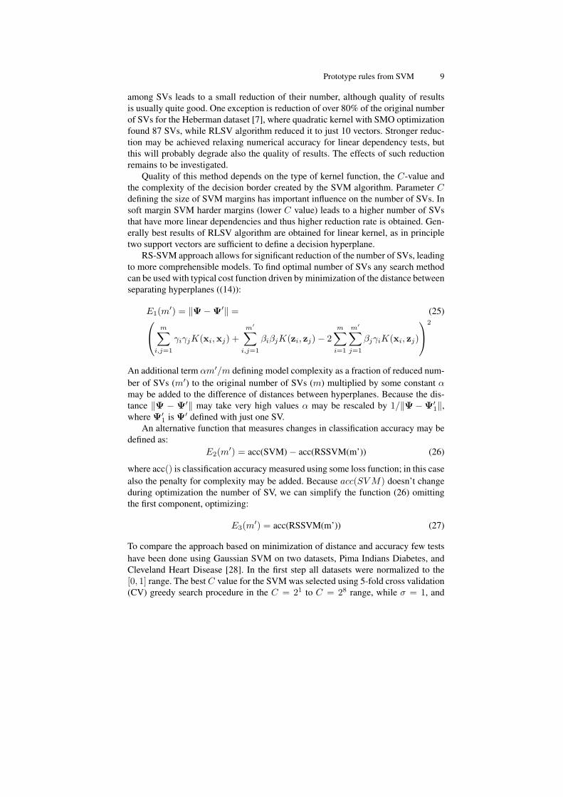
(a) Dependence of the cost function E1 on the logarithm ofthe number of SVs

100

101

102

103

0.55

0.6

0.65

0.7

0.75

0.8

(b) Dependence of the mean accuracy (cost function E3) onthe logarithm of the number of SVs. Dashed line representsmean accuracy of the original SVM

Fig. 1. Comparison of the distance (Eq. (26)) and accuracy (Eq. (27)) based cost functions forPima Indians diabetes data.

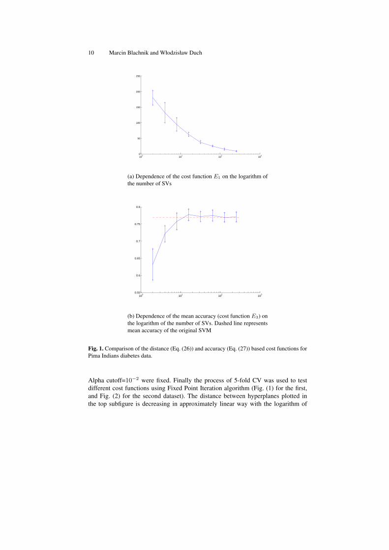
Alpha cutoff=10−2 were fixed. Finally the process of 5-fold CV was used to testdifferent cost functions using Fixed Point Iteration algorithm (Fig. (1) for the first,and Fig. (2) for the second dataset). The distance between hyperplanes plotted inthe top subfigure is decreasing in approximately linear way with the logarithm of


the number of SVs. On the other hand the classification accuracy (Eq. (27)) growsrapidly reaching the accuracy of SVM with just a few SVs.

100

101

102

103

0

50

100

150

200

250

300

(a) Dependence of the cost function E1 on the logarithm ofthe number of SVs

100

101

102

103

0.65

0.7

0.75

0.8

0.85

(b) Dependence of the mean accuracy (cost function E3) onthe logarithm of the number of SVs. Dashed line representsmean accuracy of the original SVM

Fig. 2. Comparison of the distance (Eq. (26)) and accuracy (Eq. (27)) based cost functions forCleveland Heart disease data.


Although increasing the number of SVs leads to decision border that are equiva-lent to the one found by SVM algorithm without restrictions on the number of SVsresults are not correlated with increasing accuracy of the models. Large differencesbetween hyperplanes in the region far from data are not important, but the distance-based approach does not distinguish between different regions, trying to decreasethe overall distance. This problem will be especially acute for Gaussian or othernon-linear kernels that place SV far from decision borders in the feature space. Fortwo overlapping distributions SVM with Gaussian kernels will use support vectorsthat are all around both distributions, even though only those that are close to thesupport vectors from the opposite class are really useful. It should be possible to usethe distance between closest support vectors from the opposite classes to rank can-didates for removal in the SV selection process. This can simplify the search in theaccuracy-based approach.

2.6 Problems with interpretation

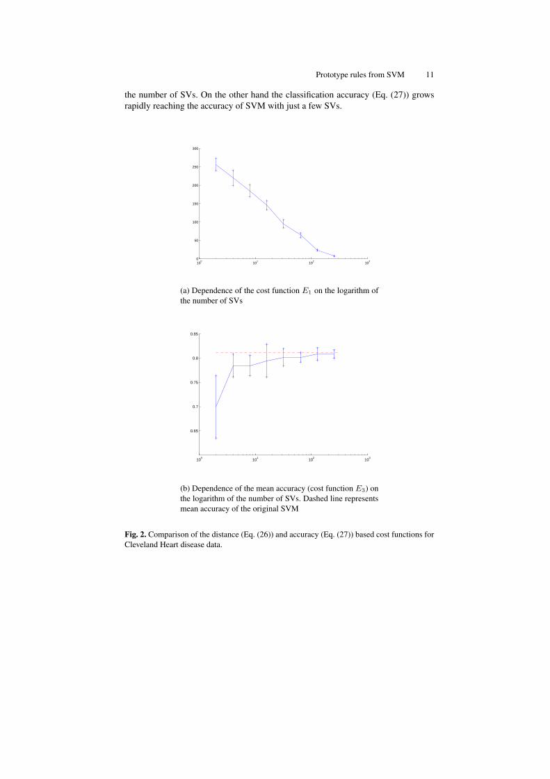
Even if a simple and transparent model that mimics SVM’s decision borders couldbe created the question “what can be learned from it” still remains. Similar prob-lems face most rule extraction approaches, including fuzzy and rough rule basedsystems, with the exception of simple crisp rule sets that sometimes have straightfor-ward interpretation [14, 19]. Prototype-based rules demand not only a small numberof prototypes but also a meaningful position of these prototypes among other inputvectors.

−1 −0.8 −0.6 −0.4 −0.2 0 0.2 0.4 0.6 0.8 1−1

−0.8

−0.6

−0.4

−0.2

0

0.2

0.4

0.6

0.8

1

(a) Contour plot of SVM classifier decision borders

None of the support vector reduction methods considered here gives prototypeswhich have simple interpretation, as they are never placed at the centers of clusters


−1 −0.8 −0.6 −0.4 −0.2 0 0.2 0.4 0.6 0.8 1−1

−0.8

−0.6

−0.4

−0.2

0

0.2

0.4

0.6

0.8

1

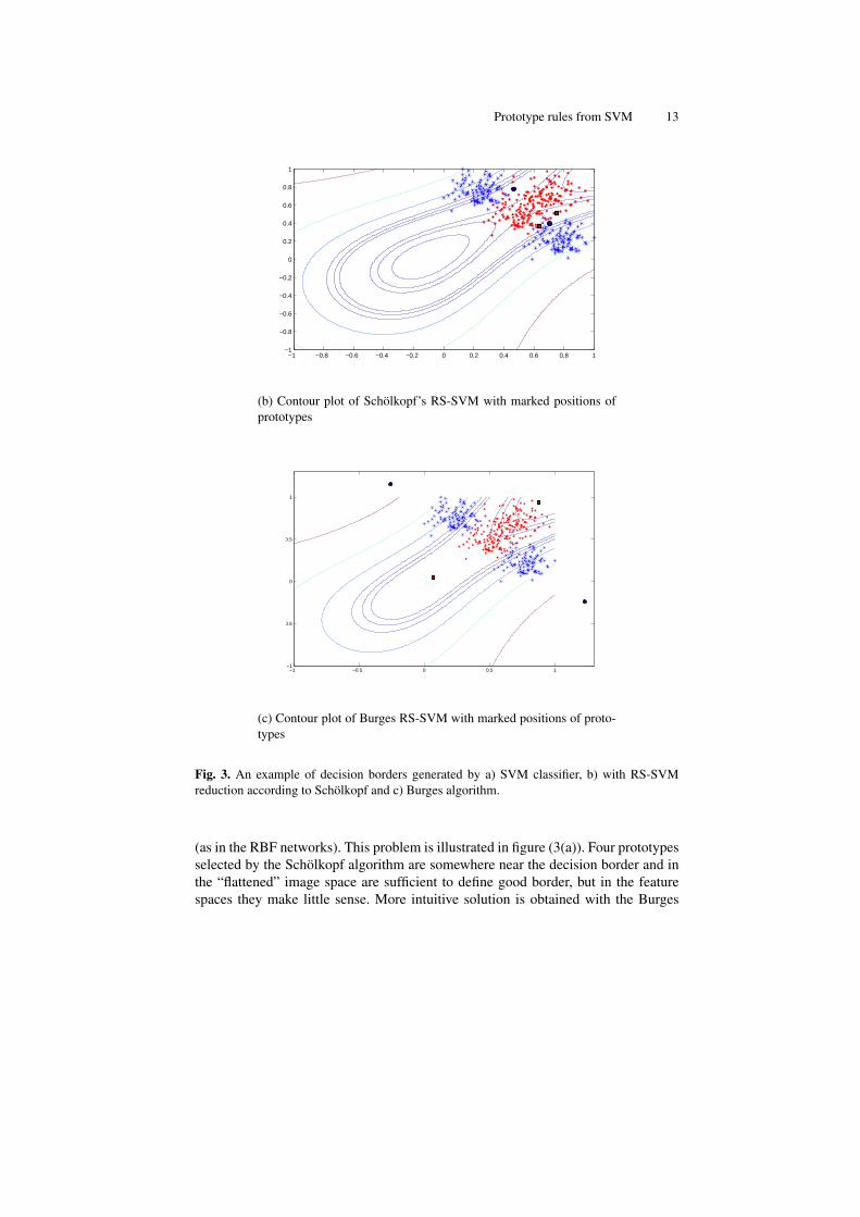
(b) Contour plot of Schölkopf’s RS-SVM with marked positions ofprototypes

−1 −0.5 0 0.5 1−1

−0.5

0

0.5

1

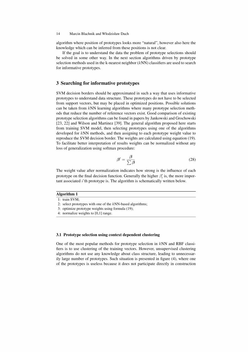
(c) Contour plot of Burges RS-SVM with marked positions of proto-types

Fig. 3. An example of decision borders generated by a) SVM classifier, b) with RS-SVMreduction according to Schölkopf and c) Burges algorithm.

(as in the RBF networks). This problem is illustrated in figure (3(a)). Four prototypesselected by the Schölkopf algorithm are somewhere near the decision border and inthe “flattened” image space are sufficient to define good border, but in the featurespaces they make little sense. More intuitive solution is obtained with the Burges


algorithm where position of prototypes looks more “natural”, however also here theknowledge which can be inferred from these positions is not clear.

If the goal is to understand the data the problem of prototype selections shouldbe solved in some other way. In the next section algorithms driven by prototypeselection methods used in the k-nearest neighbor (kNN) classifiers are used to searchfor informative prototypes.

3 Searching for informative prototypes

SVM decision borders should be approximated in such a way that uses informativeprototypes to understand data structure. These prototypes do not have to be selectedfrom support vectors, but may be placed in optimized positions. Possible solutionscan be taken from kNN learning algorithms where many prototype selection meth-ods that reduce the number of reference vectors exist. Good comparison of existingprototype selection algorithms can be found in papers by Jankowski and Grochowski[23, 22] and Wilson and Martinez [39]. The general algorithm proposed here startsfrom training SVM model, then selecting prototypes using one of the algorithmsdeveloped for kNN methods, and then assigning to each prototype weight value toreproduce the SVM decision border. The weights are calculated using equation (19).To facilitate better interpretation of results weights can be normalized without anyloss of generalization using softmax procedure:

β′ =β∑β

(28)

The weight value after normalization indicates how strong is the influence of eachprototype on the final decision function. Generally the higher β′i is, the more impor-tant associated i’th prototype is. The algorithm is schematically written below.

Algorithm 11: train SVM;2: select prototypes with one of the kNN-based algorithms;3: optimize prototype weights using formula (19);4: normalize weights to [0,1] range.

3.1 Prototype selection using context dependent clustering

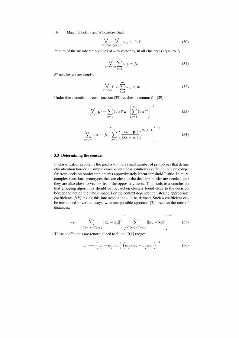
One of the most popular methods for prototype selection in kNN and RBF classi-fiers is to use clustering of the training vectors. However, unsupervised clusteringalgorithms do not use any knowledge about class structure, leading to unnecessar-ily large number of prototypes. Such situation is presented in figure (4), where oneof the prototypes is useless because it does not participate directly in construction


of the decision border. This problem may be solved with semi-supervised cluster-ing. A clustering approach which uses additional knowledge to reduce the number

0 0.1 0.2 0.3 0.4 0.5 0.6 0.7 0.8 0.9 10

0.1

0.2

0.3

0.4

0.5

0.6

0.7

0.8

0.9

1

x1 [−]

x 2 [−]

(a) Prototype selection using classi-cal clustering method (FCM)

0 0.1 0.2 0.3 0.4 0.5 0.6 0.7 0.8 0.9 10

0.1

0.2

0.3

0.4

0.5

0.6

0.7

0.8

0.9

1

x1 [−]

x 2 [−]

(b) Prototype selection using contextclustering (CFCM)

Fig. 4. Comparison of prototype selection methods using two types of clustering methods,FCM and CFCM

of prototypes was proposed by Blachnik et al. [3]. In this approach context depen-dent clustering was used to train the kNN prototypes. Context dependent clusteringis a family of grouping algorithms which use external, user defined variable (foreach input vector) describing the strengths of association between the input vectorand external parameter. Context clustering was studied by Pedrycz [31, 29], Łeski[36, 20] and others, and has been applied with very good results in training of theRBF networks [30, 1].

3.2 The conditional fuzzy clustering algorithm

One of methods that belong to the context dependent clustering family of algorithmsis Conditional Fuzzy C-Means (CFCM). It is based on minimizing cost functiondefined as:

Jm(U,P) =c∑

i=1

m∑

k=1

(uik)δ ‖xk − pi‖2A (29)

where c is the number of clusters centered at pi, m is the number of vectors, δ > 1 isa parameter describing fuzziness, and U = (uik) is a c×m dimensional membershipmatrix with elements uik ∈ [0, 1] defining the degree of membership of the k-thvector in the i-th cluster. The matrix U has to fulfill three conditions:1o each vector xk belongs to the i-th cluster to some degree:


∀1≤i≤c

∀1≤k≤m

uik ∈ [0, 1] (30)

2o sum of the membership values of k-th vector xk in all clusters is equal to fk

∀1≤k≤m

c∑

i=1

uik = fk (31)

3o no clusters are empty.

∀1≤i≤c

0 <

m∑

k=1

uik < m (32)

Under these conditions cost function (29) reaches minimum for [29], :

∀1≤i≤c

pi =m∑

k=1

(uik)δxk

[m∑

k=1

(uik)δ

]−1

(33)

∀1≤i≤c1≤k≤m

uik = fk

c∑

j=1

( ‖xk − pi‖‖xk − pj‖

)2/(δ−1)−1

(34)

3.3 Determining the context

In classification problems the goal is to find a small number of prototypes that defineclassification border. In simple cases when linear solution is sufficient one prototypefar from decision border implements approximately linear threshold P-rule. In morecomplex situations prototypes that are close to the decision border are needed, andthey are also close to vectors from the opposite classes. This leads to a conclusionthat grouping algorithms should be focused on clusters found close to the decisionborder and not on the whole space. For the context dependent clustering appropriatecoefficients f(k) taking this into account should be defined. Such a coefficient canbe introduced in various ways, with one possible approach [3] based on the ratio ofdistances:

wk =∑

j,C(xj)=C(xk)

‖xk − xj‖2 ∑

l,C(xl)6=C(xk)

‖xk − xl‖2−1

(35)

These coefficients are renormalized to fit the [0,1] range:

wk ←−(wk −min

iwi

)(max

iwi −min

iwi

)−1

(36)


Normalized wk coefficients reach values close to 0 for vectors inside large ho-mogeneous clusters, and close to 1 if the vector xk is near the vectors of the oppositeclasses and far from other vectors from the same class (for example if it is an out-lier). These normalized weights determine the external variable which then is usedto assign appropriate context or condition in the CFCM clustering process.

fk = exp(−η(wk − µ)2

)(37)

with the best parameters in the range of µ = 0.6−0.8 and η = 1−3, determined em-pirically for a wide range of datasets. The µ parameter controls where the prototypeswill be placed; for small µ they are closer to the center of the cluster and for larger µcloser to the decision borders. The range in which they are sought is determined bythe η parameter.

3.4 Numerical illustration of the CFCM approach

Conditional clustering proposed above does not use SVM to place prototypes di-rectly, but the adjustment of weights is based on the SVM decision function. Toverify this approach some simple numerical experiments were performed. Becausein the CFCM method the number of prototypes for each class has to be determinedindependently the total number of desired SVs has been divided equally among theclasses.

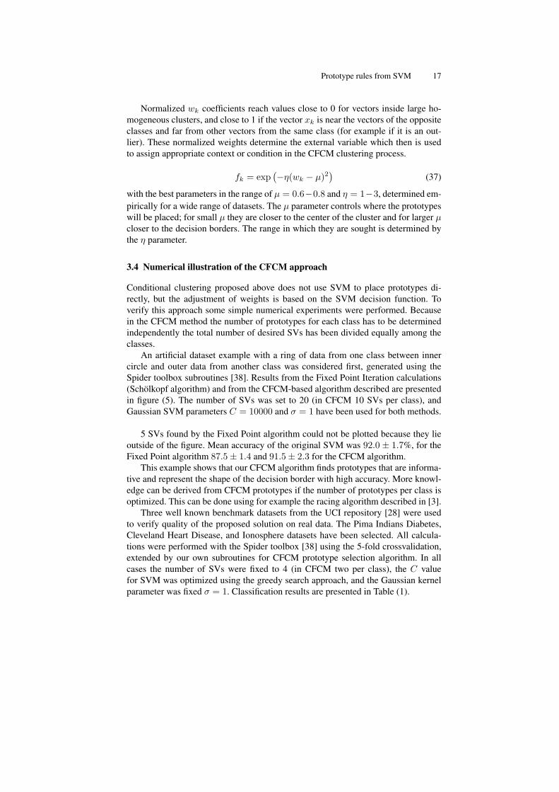
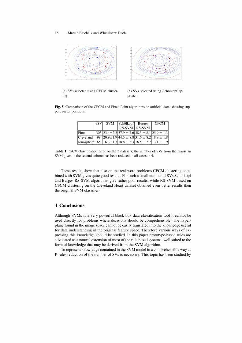
An artificial dataset example with a ring of data from one class between innercircle and outer data from another class was considered first, generated using theSpider toolbox subroutines [38]. Results from the Fixed Point Iteration calculations(Schölkopf algorithm) and from the CFCM-based algorithm described are presentedin figure (5). The number of SVs was set to 20 (in CFCM 10 SVs per class), andGaussian SVM parameters C = 10000 and σ = 1 have been used for both methods.

5 SVs found by the Fixed Point algorithm could not be plotted because they lieoutside of the figure. Mean accuracy of the original SVM was 92.0 ± 1.7%, for theFixed Point algorithm 87.5± 1.4 and 91.5± 2.3 for the CFCM algorithm.

This example shows that our CFCM algorithm finds prototypes that are informa-tive and represent the shape of the decision border with high accuracy. More knowl-edge can be derived from CFCM prototypes if the number of prototypes per class isoptimized. This can be done using for example the racing algorithm described in [3].

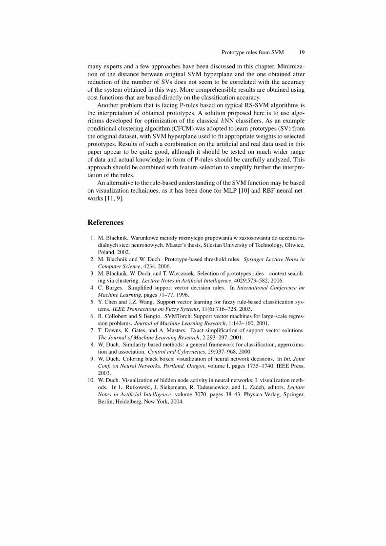
Three well known benchmark datasets from the UCI repository [28] were usedto verify quality of the proposed solution on real data. The Pima Indians Diabetes,Cleveland Heart Disease, and Ionosphere datasets have been selected. All calcula-tions were performed with the Spider toolbox [38] using the 5-fold crossvalidation,extended by our own subroutines for CFCM prototype selection algorithm. In allcases the number of SVs were fixed to 4 (in CFCM two per class), the C valuefor SVM was optimized using the greedy search approach, and the Gaussian kernelparameter was fixed σ = 1. Classification results are presented in Table (1).


−1 −0.8 −0.6 −0.4 −0.2 0 0.2 0.4 0.6 0.8 1−1

−0.8

−0.6

−0.4

−0.2

0

0.2

0.4

0.6

0.8

1

(a) SVs selected using CFCM cluster-ing

−1 −0.8 −0.6 −0.4 −0.2 0 0.2 0.4 0.6 0.8 1−1

−0.8

−0.6

−0.4

−0.2

0

0.2

0.4

0.6

0.8

1

(b) SVs selected using Schölkopf ap-proach

Fig. 5. Comparison of the CFCM and Fixed Point algorithms on artificial data, showing sup-port vector positions.

#SV SVM Schölkopf Burges CFCMRS-SVM RS-SVM

Pima 305 23.4±2.3 37.9 ± 7.6 38.3 ± 8.1 25.9 ± 1.3Cleveland 99 20.9±1.9 44.5 ± 8.8 31.6 ± 8.2 18.9 ± 1.8Ionosphere 65 6.3±1.3 18.8 ± 3.3 16.5 ± 2.7 13.1 ± 1.9

Table 1. 5xCV classification error on the 3 datasets; the number of SVs from the GaussianSVM given in the second column has been reduced in all cases to 4.

These results show that also on the real-word problems CFCM clustering com-bined with SVM gives quite good results. For such a small number of SVs Schölkopfand Burges RS-SVM algorithms give rather poor results, while RS-SVM based onCFCM clustering on the Cleveland Heart dataset obtained even better results thenthe original SVM classifier.

4 Conclusions

Although SVMs is a very powerful black box data classification tool it cannot beused directly for problems where decisions should be comprehensible. The hyper-plane found in the image space cannot be easily translated into the knowledge usefulfor data understanding in the original feature space. Therefore various ways of ex-pressing this knowledge should be studied. In this paper prototype-based rules areadvocated as a natural extension of most of the rule based systems, well suited to theform of knowledge that may be derived from the SVM algorithm.

To represent knowledge contained in the SVM model in a comprehensible way asP-rules reduction of the number of SVs is necessary. This topic has been studied by


many experts and a few approaches have been discussed in this chapter. Minimiza-tion of the distance between original SVM hyperplane and the one obtained afterreduction of the number of SVs does not seem to be correlated with the accuracyof the system obtained in this way. More comprehensible results are obtained usingcost functions that are based directly on the classification accuracy.

Another problem that is facing P-rules based on typical RS-SVM algorithms isthe interpretation of obtained prototypes. A solution proposed here is to use algo-rithms developed for optimization of the classical kNN classifiers. As an exampleconditional clustering algorithm (CFCM) was adopted to learn prototypes (SV) fromthe original dataset, with SVM hyperplane used to fit appropriate weights to selectedprototypes. Results of such a combination on the artificial and real data used in thispaper appear to be quite good, although it should be tested on much wider rangeof data and actual knowledge in form of P-rules should be carefully analyzed. Thisapproach should be combined with feature selection to simplify further the interpre-tation of the rules.

An alternative to the rule-based understanding of the SVM function may be basedon visualization techniques, as it has been done for MLP [10] and RBF neural net-works [11, 9].

References

1. M. Blachnik. Warunkowe metody rozmytego grupowania w zastosowaniu do uczenia ra-dialnych sieci neuronowych. Master’s thesis, Silesian University of Technology, Gliwice,Poland, 2002.

2. M. Blachnik and W. Duch. Prototype-based threshold rules. Springer Lecture Notes inComputer Science, 4234, 2006.

3. M. Blachnik, W. Duch, and T. Wieczorek. Selection of prototypes rules – context search-ing via clustering. Lecture Notes in Artificial Intelligence, 4029:573–582, 2006.

4. C. Burges. Simplified support vector decision rules. In International Conference onMachine Learning, pages 71–77, 1996.

5. Y. Chen and J.Z. Wang. Support vector learning for fuzzy rule-based classification sys-tems. IEEE Transactions on Fuzzy Systems, 11(6):716–728, 2003.

6. R. Collobert and S Bengio. SVMTorch: Support vector machines for large-scale regres-sion problems. Journal of Machine Learning Research, 1:143–160, 2001.

7. T. Downs, K. Gates, and A. Masters. Exact simplification of support vector solutions.The Journal of Machine Learning Research, 2:293–297, 2001.

8. W. Duch. Similarity based methods: a general framework for classification, approxima-tion and association. Control and Cybernetics, 29:937–968, 2000.

9. W. Duch. Coloring black boxes: visualization of neural network decisions. In Int. JointConf. on Neural Networks, Portland, Oregon, volume I, pages 1735–1740. IEEE Press,2003.

10. W. Duch. Visualization of hidden node activity in neural networks: I. visualization meth-ods. In L. Rutkowski, J. Siekemann, R. Tadeusiewicz, and L. Zadeh, editors, LectureNotes in Artificial Intelligence, volume 3070, pages 38–43. Physica Verlag, Springer,Berlin, Heidelberg, New York, 2004.


11. W. Duch. Visualization of hidden node activity in neural networks: Ii. application to rbfnetworks. In L. Rutkowski, J. Siekemann, R. Tadeusiewicz, and L. Zadeh, editors, Lec-ture Notes in Artificial Intelligence, volume 3070, pages 44–49. Physica Verlag, Springer,Berlin, Heidelberg, New York, 2004.

12. W. Duch, R. Adamczak, and G. H. F. Diercksen. Distance-based multilayer perceptrons.In M. Mohammadian, editor, International Conference on Computational Intelligence forModelling Control and Automation, pages 75–80, Amsterdam, The Netherlands, 1999.IOS Press.

13. W. Duch, R. Adamczak, and G.H.F. Diercksen. Classification, association and patterncompletion using neural similarity based methods. Applied Mathemathics and ComputerScience, 10:101–120, 2000.

14. W. Duch, R. Adamczak, and K. Grabczewski. A new methodology of extraction, opti-mization and application of crisp and fuzzy logical rules. IEEE Transactions on NeuralNetworks, 12:277–306, 2001.

15. W. Duch and M. Blachnik. Fuzzy rule-based systems derived from similarity to proto-types. In N.R. Pal, N. Kasabov, R.K. Mudi, S. Pal, and S.K. Parui, editors, Lecture Notesin Computer Science, volume 3316, pages 912–917. Physica Verlag, Springer, New York,2004.

16. W. Duch and G. H. F. Diercksen. Feature space mapping as a universal adaptive system.Computer Physics Communications, 87:341–371, 1995.

17. W. Duch and K. Grudzinski. Prototype based rules - new way to understand the data. InIEEE International Joint Conference on Neural Networks, pages 1858–1863, WashingtonD.C, 2001. IEEE Press.

18. W. Duch and K. Grudzinski. Meta-learning via search combined with parameter opti-mization. In L. Rutkowski and J. Kacprzyk, editors, Advances in Soft Computing, pages13–22. Physica Verlag, Springer, New York, 2002.

19. W. Duch, R. Setiono, and J. Zurada. Computational intelligence methods for understand-ing of data. Proceedings of the IEEE, 92(5):771–805, 2004.

20. J. Łeski. Ordered weighted generalized conditional possibilistic clustering. In J. Chojcanand J. Łeki, editors, Zbiory rozmyte i ich zastosowania, pages 469–479. WydawnictwaPolitechniki Slaskiej, Gliwice, 2001.

21. K. Grabczewski and W. Duch. Heterogeneous forests of decision trees. Springer LectureNotes in Computer Science, 2415:504–509, 2002.

22. M. Grochowski and N. Jankowski. Comparison of instance selection algorithms. ii. resultsand comments. Lecture Notes in Computer Science, 3070:580–585, 2004.

23. N. Jankowski and M. Grochowski. Comparison of instance selection algorithms. i. algo-rithms survey. Lecture Notes in Computer Science, 3070:598–603, 2004.

24. T. Joachims. Learning to Classify Text Using Support Vector Machines. Kluwer AcademicPublisher, 2002.

25. L.I. Kuncheva and J.C. Bezdek. An integrated framework for generalized nearest proto-type classifier design. International Journal of Uncertainty, 6(5):437–457, 1998.

26. J.T. Kwok and I.W. Tsang. The pre-image problem in kernel methods. IEEE Transactionson Neural Networks, 15:408–415, 2003.

27. K. Lin and C. Lin. A study on reduced support vector machines. IEEE Transactions onNeural Networks, 14(6):1449–1459, 2003.

28. C.J. Merz and P.M. Murphy. UCI repository of machine learning databases, 1998-2004.http://www.ics.uci.edu/∼mlearn/MLRepository.html.

29. W. Pedrycz. Conditional fuzzy c-means. Pattern Recognition Letters, 17:625–632, 1996.30. W. Pedrycz. Conditional fuzzy clustering in the design of radial basis function neural

networks. IEEE Transactions on Neural Networks, 9(4), 1998.


31. W. Pedrycz. Fuzzy set technology in knowledge discover. Fuzzy Sets and Systems,98(3):279–290, 1998.

32. E. Pekalska and R.P.W. Duin. The dissimilarity representation for pattern recognition:foundations and applications. New Jersey; London: World Scientific, 2005.

33. J. Platt. Using sparseness and analytic qp to speed training of support vector machines.Advances in Neural Information Processing Systems, 11, 1999.

34. I. Roth and V. Bruce. Perception and Representation. Open University Press, 1995. 2nded.

35. B. Schölkopf, P. Knirsch, A. Smola, and C. Burges. Fast approximation of support vectorkernel expansions. Informatik Aktuell, Mustererkennung, 1998.

36. J. Łeski. A new generalized weighted conditional fuzzy clustering. BUSEFAL, 81:8–16,2000.

37. T. Takagi and M. Sugeno. Fuzzy identification of systems and its applications to modeling and control. IEEE Transactions on Systems, Man, Cybernetics, 15:116–132, 1985.

38. J. Weston, A. Elisseeff, G. BakIr, and F. Sinz. The spider.http://www.kyb.tuebingen.mpg.de/bs/people/spider/.

39. D.R. Wilson and T.R. Martinez. Reduction techniques for instance-based learning algo-rithms. Machine Learning, 38:257–268, 2000.

prototype rules from svm

Documents