validation of wet gas surge phenomena - ntnu open
TRANSCRIPT
Validation of Wet Gas Surge Phenomena
Lars Andreas Øvrum Sørvik
Master of Energy and Environmental Engineering
Supervisor: Lars Erik Bakken, EPTCo-supervisor: Trond Gruner, EPT
Øyvind Hundseid, EPT
Department of Energy and Process Engineering
Submission date: June 2012
Norwegian University of Science and Technology


Preface and Acknowledgments
I
Preface and Acknowledgments
This master's thesis concludes my NTNU Master of Science degree program at the
department of energy and process engineering.
I would like to thank my supervisor Lars Erik Bakken for all the help in connection with my
master thesis with excellent guidance and for a very interesting year. I would also like to
thank my fellow students at the office 501 for social cohesion and technical discussions that
have stimulated to a good learning environment. PhD Øyvind Hundseid for guidance and Lars
Konrad for the implementation of the measuring devices in the test rig. Last but not least, I
want to thank PhD and researcher Trond Gammelsæter Grüner who has been of invaluable
help during the project work. You have all been of great importance for me and my master’s
thesis.
_______________________________________
Lars Andreas Øvrum Sørvik
Trondheim, June 13, 2012

Preface and Acknowledgments
II
Abstract
III
Abstract
In order to utilize the fossil resources on the Norwegian continental shelf, technology and
expertise have proven to be of great importance and hence, essential for further exploration
and development of new resources. A key element in this matter is the subsea wet gas
compression technology which enables the transport of well stream directly to a land based
treatment system, or more remote processing facilities offshore. Compression of gas at the
seabed is a significant technology advance no one has previously made. The technology of
subsea gas compression is one of the most important measures to deliver increased volumes
from existing gas fields as well as developing resources in more remote and vulnerable areas.
Due to the need of expertise and development of subsea installations, in order to meet the
demand for fossil fuels and be competitive in a constantly increasing market, the Norwegian
University of Science and Technology (NTNU) has built an experimental rig to test a wet gas
compressor. The rig is unique and important to analyze the basic mechanisms and occurrence
of instabilities related to wet gas compression. Both the literature review and the experimental
work presented here are performed in order to visualize and document instabilities related to
the phenomena surge and stall. Experimental data in this master thesis are obtained from a
one- stage wet gas centrifugal compressor with an axial direct inlet. The stage involves a
shrouded impeller, a vaneless diffuser and a volute. The compressor is a part of an open loop
facility that is located at NTNU in Trondheim. The test rig is designed to operate with
different amounts of liquid in the gas with gas volume fractions (GVF) and gas mass fractions
(GMF) down to correspondingly 0.95 and 0.5. Applications in LabView were made and
designed to analyze the raw data from the pressure sensors and pitot tubes in order to post-
process and represent the data in a graphical manner. Log files from a total of seven scientific
experiments with dry- and wet gas were documented and analyzed to identify the impeller
outlet angle and achieving a more precise identification of wet gas surge initiation and
instability precursor.
The steady state flow angle experiments revealed a stringent increase in flow angle with
decreasing volume flow, for both the dry gas test of 10000 and 9000 rpm, with maximum
corresponding flow angles of 81.5 and 86 degrees. A sudden rise in flow angle gradient was
found to occur at a volume flow of 0.95 m3/s and 0.8 m
3/s for 10000 rpm and 9000 rpm,
respectively, due to the volute causing a shift change from deceleration to acceleration
performance, at the respective volume flows. Flow angle measurements of dry gas were
further validated and compared with Matlab and CFD simulation revealing coincident trends.
The performed wet gas tests were associated with a greater uncertainty than dry gas, due to
the influence of liquid. However, the wet gas curves showed distinct trends with lower
discharge angles across the spectrum compared to the case for dry gas measurements.
The transient surge identification test was conducted on 7500 rpm with alternating GMF in
the range from 0.6 to 0.42. The pressure characteristic revealed the first sign of intermittent
behavior at a volume flow of 0.26 m3/s prevailing sudden stringent static pressure
fluctuations. The corresponding frequency spectrum for dynamic pressure sensors shows that
the critical disturbance occurs, and is enhanced at low frequencies causing the initiation of
surge at a volume flow of 0.27 m3/s. A pitot tube set-up for identification of surge onset was
evaluated and compared to the measurements conducted by a static pressure-, a differential
pressure- and a high responsive dynamic pressure sensor. The detection tube indicated a
possible precursor to surge by prevailing change and high fluctuations in the stagnation
pressure.

Abstract
IV
Observation through the impeller inlet showed that an annular backflow ring was formed with
decreasing volume flow. The first observation of the ring shape was done for a volume flow
of 0.3 m3/s, followed by larger developments and a chaotic flow path with complete backflow
for volume flow lower than 0.25 m3/s.
Sammendrag
V
Sammendrag
For å utnytte fossile ressursene på norsk kontinentalsokkel, har teknologi og kompetanse vist
seg å være av stor betydning og viktig for videre utforskning samt utvikling av nye ressurser.
Et sentralt element i dette er havbunns våtgass kompresjon teknologi som muliggjør transport
av brønnstrøm direkte til et landbasert prosess anlegg, eller mer fjerntliggende prosessanlegg
til havs. Kompresjon av gass på havbunnen er en viktig teknologi ingen tidligere har gjort.
Teknologien ved undervanns gasskompresjon er en av de viktigste tiltakene for å levere økt
volum fra eksisterende gassfelt, samt utvikle ressurser i mer fjerntliggende og sårbare
områder.
På grunn av behovet for kompetanse og utvikling av havbunns installasjoner, for å møte
etterspørselen etter fossilt brennstoff og være konkurransedyktig i et stadig økende marked;
har NTNU bygget en eksperimentell rigg for å teste en våt gass kompressor. Riggen er unik
og et viktig verktøy for å analysere de grunnleggende mekanismer og forekomst av ustabilitet
knyttet til våtgass kompresjon. Både litteratur og eksperimentelt arbeid presenteres her og er
utført for å visualisere og dokumentere ustabiliteter knyttet til fenomener «surge» og «stall».
Eksperimentelle data i denne masteroppgaven er hentet fra en ett-trinns våtgass sentrifugal
kompressor med en aksial direkte inntak. Kompressor trinnet består av en shrouded impeller,
en vaneless diffusor og en volute. Kompressoren er konstruert for å operere med ulike
mengder væske i gassen med gass volum fraksjoner (GVF) og gass masse fraksjoner (GMF)
ned til korresponderende 0,95 og 0,5. LabView programmer ble benyttet og designet for å
analysere rådata fra trykksensorer og pitot-rør for å kunne behandle og representere dataene
på en grafisk måte. Loggfiler fra sju vitenskapelige eksperimenter med tørr- og våtgass ble
dokumentert og analysert for å identifisere impeller utløps vinkel og oppnå en mer presis
identifisering av våtgass «surge» initiering og forløper til denne ustabiliteten.
Steady state strømningsvinkel eksperimenter viste en stringent økning i strømningsvinkel med
avtagende volum strøm, for tørrgass testen med 10000 og 9000 rpm, med maksimale
korresponderende strømningsvinkler på 81,5 og 86 grader. En plutselig økning i
strømningsvinkel gradient ble funnet å skje ved en volumstrøm på 0,95 m3 / s og 0,8 m3 / s
for henholdsvis10000- og 9000 rpm, på grunn av at voluten forårsaker en endring fra
nedbremsing til akselerasjon ytelse, ved de respektive volum strømmene. Strømningsvinkel
målinger av tørr gass ble ytterligere validert og sammenlignet med Matlab og CFD simulering
som viste sammenfallende trender. De utførte våtgass tester var assosiert med en større
usikkerhet enn tørr gass, på grunn av innflytelsen av væske. Imidlertid viste våtgass kurvene
tydelige trender med lavere vinkler over hele spekteret i forhold til tørrgass målinger.
En transient surge test ble utført på 7500 rpm med vekslende GMF i området fra 0,6 til 0,42.
Trykk karakteristikken avslørte det første tegnet på ujevn atferd på en volumstrøm på 0,26
m3/s med plutselige statiske trykksvingninger. Det tilsvarende frekvensspekteret for
dynamiske trykksensorer viste at kritiske forstyrrelse oppstår, og forsterkes ved lave
frekvenser som forårsaker initiering av surge ved en volumstrøm på 0,27 m3
/ s. Et pitotrør for
identifisering av surge ble evaluert og sammenlignet med målingene utført av en statisk trykk-
, en differansetrykk-og en høy responsiv dynamisk trykksensor. Påvisning fra pitot røret
indikerte en mulig forløper til surge med gjeldende endring og høye svingninger i stagnasjon
trykket. Observasjon gjennom impeller innløpet viste at en ringformet tilbakestrøm ble dannet
med avtagende volum flyt. Den første observasjonen av ring formen ble gjort for en

Sammendrag
VI
volumstrøm på 0,3 m3
/ s, etterfulgt av større ringdannelser og komplett tilbakestrøm for
volumstrøm lavere enn 0,25 m3
/ s.
Table of Contents
VII
Table of Contents
Preface and Acknowledgments ................................................................................................... I
Abstract .................................................................................................................................... III
Sammendrag .............................................................................................................................. V
Table of Contents ....................................................................................................................... 7
List of Figures ............................................................................................................................ 9
List of Tables ............................................................................................................................ 10
Nomenclature ........................................................................................................................... 11
1 Introduction ........................................................................................................................ 1
1.1 Background .................................................................................................................. 1
1.2 Multiphase compression concepts ............................................................................... 2
1.3 Project scope ................................................................................................................ 3
1.4 Report structure ........................................................................................................... 3
2 Test rig facility ................................................................................................................... 5
2.1 Main facility data ......................................................................................................... 5
2.2 Compressor data .......................................................................................................... 6
2.3 Instrumentation ............................................................................................................ 7
2.4 Chapter summary and conclusion ................................................................................ 8
3 Multiphase flow .................................................................................................................. 9
3.1 Multiphase fundamentals ............................................................................................. 9
3.2 Multiphase effects on the boundary layer .................................................................. 13
3.3 Chapter summary and conclusion .............................................................................. 14
4 Aerodynamic in centrifugal compressor .......................................................................... 15
4.1 Shrouded impeller ...................................................................................................... 15
4.1.1 Impeller flow patterns ........................................................................................ 17
4.2 Impeller and diffuser interactions .............................................................................. 19
4.3 Vaneless diffuser ....................................................................................................... 22
4.3.1 Diffuser flow patterns ......................................................................................... 22
4.4 Wet gas implementation ............................................................................................ 27
5 Aerodynamic instabilities for dry gas .............................................................................. 29
5.1 Compressor instability for dry gas ............................................................................. 29
5.2 Rotating stall .............................................................................................................. 32
5.3 Boundary Layer development and separation ........................................................... 32
5.4 Impeller rotating stall ................................................................................................. 36
5.5 Vaneless diffuser rotating stall .................................................................................. 37
Table of Contents
VIII
5.6 Surge .......................................................................................................................... 40
5.7 Chapter summary and conclusion .............................................................................. 43
6 The influence of wet gas for compressor stability ........................................................... 45
6.1 Fogging and heavy rain ingestion for axial compressors .......................................... 45
6.2 Wet gas centrifugal compressor stability ................................................................... 46
7 Flow visualization techniques .......................................................................................... 49
7.1 Pitot probe investigation ............................................................................................ 50
7.1.1 Pitot tube fundamentals and measurement principles ........................................ 50
7.1.2 Pitot tube for turbo machinery applications ....................................................... 53
7.1.3 Pitot probes for wet gas measurements in the NTNU impeller rig. ................... 55
7.2 Pitot- based measuring devices .................................................................................. 55
7.2.1 Fast- Response Aerodynamic Probe measurement system ................................ 55
7.2.2 Multi hole probe technology .............................................................................. 57
7.3 Chapter summary and conclusion .............................................................................. 59
8 Description of experimental setup and procedure ............................................................ 61
8.1 Summary previous work ............................................................................................ 61
8.2 Focus of experiment .................................................................................................. 61
8.3 Installation of Pitot –static probe in diffuser wall ..................................................... 62
8.4 Installation of the surge detection tube ...................................................................... 64
8.5 Chapter summary and conclusion .............................................................................. 65
9 Experimental results and discussion ................................................................................ 67
9.1 Diffuser pattern investigation .................................................................................... 67
9.1.1 Dry gas flow angle ............................................................................................. 67
9.1.2 Comparison between Laboratory measurements and Matlab simulations ......... 71
9.1.3 Comparison between Laboratory measurements and CFD simulations ............ 73
9.1.4 Wet gas flow angle ............................................................................................. 75
9.1.5 Comparison between wet and dry gas ................................................................ 76
9.2 Impeller surge detection ............................................................................................ 77
9.2.1 Transient wet gas performance characteristic .................................................... 77
9.2.2 Pressure surge detection and identification measurements ................................ 81
9.2.3 Visual observation of surge ................................................................................ 83
10 Discussion ........................................................................................................................ 85
Flow angle investigation ...................................................................................................... 85
Wet gas surge detection ........................................................................................................ 85
11 Recommendations for further work ................................................................................. 87
Flow angle investigation ...................................................................................................... 87
Table of Contents
IX
Wet gas surge detection ........................................................................................................ 87
References ................................................................................................................................ 89
Appendix A: Supplementary experimental graphs and figures................................................ 93
Appendix A.1 Frequency spectrums at 7500 rpm for wet gas ............................................. 93
Appendix A.2 Identification of Surge .................................................................................. 95
Appendix A.3 Visual Surge detection .................................................................................. 97
Appendix B: Technical drawings of the impeller rig ............................................................... 98
Appendix C: Instrumentation data sheets ............................................................................... 100
Appendix D: Risk assessment report ..................................................................................... 102
Appendix E: Gantt chart ......................................................................................................... 104
List of Figures
Figure 2-1: Compressor test rig facility ..................................................................................... 5 Figure 2-2: Liquid injection module with transparent inlet section and diffuser plexiglas. ...... 6
Figure 2-3: Basic schematic of the impeller rig ......................................................................... 7 Figure 2-4: Positioning of PCB sensors. .................................................................................... 7
Figure 3-1: Multiphase relative speed of sound in air-water at 1 bar (Wood’s model) [5]...... 10 Figure 3-2: Flow regimes for different gas and liquid velocities [6]. ...................................... 11
Figure 3-3: Sketch of annular flow. ......................................................................................... 12 Figure 3-4: Boundary development of an airfoil ...................................................................... 13 Figure 4-1: Centrifugal compressor (NTNU Impeller test rig). ............................................... 15
Figure 4-2: Impeller with backswept vanes. ............................................................................ 16 Figure 4-3: Flow map of impeller plane (blade to blade) [13]. ................................................ 17
Figure 4-4: Flow map as seen in meridional plene( hub to shroud ) [13] ................................ 18 Figure 4-5: Boundary-layer development ................................................................................ 19
Figure 4-6: Effects on velocity triangles by various parameters[13]. ...................................... 20 Figure 4-7: Jet-wake distribution from an impeller [13] .......................................................... 21
Figure 4-8: Tangential and radial direction in diffuser flow .................................................... 24 Figure 4-9: Diffuser performance with good performance. ..................................................... 25 Figure 4-10 : Actual measured boundary layer separation and poor performance. ................. 25 Figure 4-11:Cross section view of the diffuser and volute for 0.85m
3/s at 9000 rpm [19] ...... 26
Figure 4-12:Computional Fluid Dynamic (CFD) velocity and pressure simulation of the
diffuser and volute[19]. ............................................................................................................ 26 Figure 4-13: Computional Fluid Dynamic (CFD) velocity simulation of the diffuser [5]. ..... 27 Figure 4-14: Particle simulation on the impeller rig for 0.96 m
3/s at 9000 rpm[19, 20]......... 28
Figure 5-1: Progressiv throttling on a compressor test rig [22]. .............................................. 30 Figure 5-2: Centrifugal compressor characteristic. .................................................................. 31
Figure 5-3: Separation of the boundary layer and vortex formation at a circular cylinder[8] . 33 Figure 5-4: Boundary layer flow close to the separation point S [8] ....................................... 33
Figure 5-5: Diffuser flow with good performance. .................................................................. 34 Figure 5-6 : Actual measured boundary layer separation with poor performance. .................. 34 Figure 5-7: Separation over a wing profile with increasing attack angles [8]. ........................ 35 Figure 5-8: Laminar versus turbulent boundary layer [8]. ....................................................... 35
Table of Contents
X
Figure 5-9: Stall affects adjacent blades[12]. ........................................................................... 36 Figure 5-10: Effect of inlet Mach number on critical flow angle [28]. .................................... 38 Figure 5-11: Vaneless diffuser stability [30]. ........................................................................... 39 Figure 5-12: Surge cycle .......................................................................................................... 40
Figure 5-13: Flow trajectory in the diffuser. ............................................................................ 41 Figure 5-14: Basic compression system[23]. ........................................................................... 42 Figure 7-1: Pitot static probe. ................................................................................................... 51 Figure 7-2: Pitot tube ................................................................................................................ 51 Figure 7-3: Pitot tube rake geometry [49]. ............................................................................... 52
Figure 7-4: Averaging Pitot tube [49]. ..................................................................................... 53 Figure 7-5: FRAP probe configurations ................................................................................... 57 Figure 7-6: FRAP probe configurations ................................................................................... 57
Figure 7-7: Position I ................................................................................................................ 57 Figure 7-8: Three- hole probe in a incoming flow field ........................................................... 58 Figure 8-1: Mounting and localization of the pitot tube. ......................................................... 62 Figure 8-2: Sketch of the pitot- probe positioning ................................................................... 63
Figure 8-3: Protractor set-up and signal generator ................................................................... 64 Figure 8-4: Section of a CAD drawing given from Appendix B2. .......................................... 64 Figure 9-1: Flow angles at 10000 rpm dry gas ......................................................................... 68 Figure 9-2: Impeller and diffuser characteristic for 10000 and 9000 rpm [62] ....................... 69
Figure 9-3: Flow angles at 9000 rpm dry gas ........................................................................... 70 Figure 9-4: Flow angles for 10000 and 9000 rpm .................................................................... 71 Figure 9-5: Matlab and lab flow angle comparison at 10000 rpm. .......................................... 72
Figure 9-6: Simulation domain where the pitot measurements are conducted [20] ................. 73
Figure 9-7: CFD and Lab flow angle comparison at 9000 rpm ............................................... 74 Figure 9-8: CFD and Lab flow angle comparison at 10000 rpm ............................................. 74 Figure 9-9: Wet gas flow angle measurements ........................................................................ 76
Figure 9-10: Flow angle comparison between Dry and wet gas .............................................. 77 Figure 9-11: Pressure characteristic for wet gas at 7500 rpm .................................................. 78
Figure 9-12: Volume flow characteristic for wet gas at 7500 rpm .......................................... 79 Figure 9-13: Transient GMF change for wet gas at 7500 rpm ................................................. 79 Figure 9-14: Frequency spectrum for wet gas at 7500 rpm for sensor channel 20 .................. 80
Figure 9-15: Frequency spectrum for wet gas at 7500 rpm for sensor channel 22 .................. 81 Figure 9-16: Pressure characteristic into surge, channel 27 ..................................................... 82
Figure 9-17: Comparison of pressure characteristics into surge for various channels ............. 82 Figure 9-18: Visual observation of annulus ring of reversed flow .......................................... 83
List of Tables
Table 2-1: Compressor parameters. ........................................................................................... 6 Table 2-2: Maximum uncertainty. .............................................................................................. 8
Table 9-1: Test matrix steady state dry gas .............................................................................. 67 Table 9-2: Flow angle devation between CFD and laboratory measurements......................... 75 Table 9-3: Test matrix steady state wet gas ............................................................................. 75
Table 9-4: Test matrix for transient wet gas............................................................................. 78
Table of Contents
XI
Nomenclature
Abbreviations and acronyms
CFD Computional Fluid Dynamics
ETH Eidgenössische Technische Hochschule
FA Film Anemometry
FFT Fast Fourier Transform
GE General Electric
GMF Gas Mass Fraction
GVF Gas Volume Fraction
HV High Voltage
HWA Hot-Wire Anemometry
LDV Laser Doppler Velocimetry
MAE Mean Absolute Error
MHP Multi-Hole probe
FRAP Fast Responsive Aerodynamic Probe
L2F Laser two-focused Velocimetry
MHP Multi Hole Probe
NTNU Norwegian University of Science and
Technology
PCB PicoCoulomB
PIV Particle Image Velocimetry
PSP Pressure Sensitive Paint
PXI PCI Extensions for Instrumentation
RPM Rotations Per Minute
UPS Uninterruptible Power Supply
VDC Volts of Direct Current
Greek letters
α Flow angle [degree]
α' Measured flow angle [degree]
β Flow angle [degree]
β' Angle between center radius to pitot
position
[degree]
tpP The total dynamic head (droplet) []
T PP The total dynamic head []
T PMP The total homogenous dynamic head []
Density [kg/m3]
* Density ratio [-]
Slip factor [-]
Shear stress [kg/ms2]
Table of Contents
XII
Roman letters and expression
a Speed of sound [m/s]
B Greitzer parameter [-]
b Width [mm]
C Actual flow velocity [m/s]
*C Calibration constant [-]
2C Tangential absolute velocity with
finite number of blades
[m/s]
2C Tangential component with infinite
number of blades
[m/s]
H Hold-up [-]
L Length [mm]
N Number of blades [-]
Mass flow [kg/s ]
Ma Mach number [-]
Q Volume flow [m3/s
]
r Radius [mm]
R Length between impeller center and
pitot tube center
[mm]
Re Reynolds number [-]
r Length of pitot “foot” [mm]
U Impeller tip velocity [m/s]
v Volume [m2]
VSG Superficial gas velocity [m/s]
VSL Superficial liquid velocity [m/s]
x Distance [mm]
X Laminar turbulent transition point [-]
Subscripts
1 Impeller inlet
2 Impeller outlet/diffuser inlet
3 Diffuser outlet
C Compressor
c Critical
CR Cross- section
d Droplet
DP Dynamic pressure
L logarithmic
Liquid
F Film
Gas
h Consistent density
H Hub
HR Helmholtz resonator
S Shroud
p Plenum
t Throttle

Table of Contents
XIII
r Ratio
m Mixture
w Wall

Table of Contents
XIV
Introduction
1
1 Introduction
1.1 Background
Norway is the seventh largest oil exporter in the world and the second largest exporter of
natural gas to Europe. Despite the fact that oil production has declined since its peak in 2001
the total production is still high due to increased gas production. Historically new production
capacity has come from the development of large oil/gas fields. Over the last five years a
significant portion of new production capacity has come from few large projects. In the future
a change towards more but smaller fields is expected. However, the recent Skrugaard/Havis
discovery in the Barents Sea and the Johan Sverdrup discovery in the North Sea represent
significant new opportunities. Together with the potential for improved recovery from
existing fields the new discoveries are important for the long term perspective with substantial
production on the Norwegian continental shelf [1].
In order to utilize the fossil resources on the Norwegian continental shelf, technology and
expertise have proven to be of great importance and hence, essential for further exploration
and development of new resources. A continued focus on research, development and
implementation of new technology are therefore regarded critical to future value creation.
Recent attention has shifted towards smaller and more remote fields with limited
infrastructure. As a consequence development and operation of such fields requires new cost
effective technology [1].
A key element in this matter is the subsea wet gas compression technology which enables the
transport of well stream directly to a land based treatment system, or more remote processing
facilities offshore. The technology may in some cases eliminate the need for offshore
processing facilities, which can contribute to a remarkable cost reduction. Most suppliers of
turbo machinery are thereby investing in the development of sea-floor-based wet gas
compressors. Subsea compression is a ground-breaking technology representing a paradigm
shift for the oil and gas industry [1].
Statoils ultimate vision is a complete subsea factory on the sea floor within 2020 which could
be a potential game changer in future arctic field development under ice far from shore. In
that context subsea compression is extremely important. The slogan “ longer, deeper and
colder “ is used by Statoil to emphasize on longer from shore, deeper waters and colder
environment [2].
Due to the need of expertise and development of subsea installations, in order to meet the
demand of fossil fuels and be competitive in a constantly increasing market, NTNU has built
an experimental rig to test a wet gas compressor. The rig is unique and important to analyze
the basic mechanisms and occurrence of instabilities related to wet gas compression. This is
what the master thesis is about.
Introduction
2
1.2 Multiphase compression concepts
Compression of gas at the seabed is a significant technology advance no one has previously
developed. The technology of subsea gas compression is one of the most important measures
to deliver increased volumes from existing gas fields as well as developing resources in more
remote and vulnerable areas. When the pressure in the reservoirs declines the flow become
unstable and the drive mechanisms i.e. well pressure becomes too weak to transport the gas.
The closer the compressor is to the wellhead the higher the efficiency, production rates and
total recovery become.
On the Norwegian Continental shelf there are currently 4 subsea gas compression projects
going on with different maturity. Åsgard subsea gas compression, Gullfaks subsea wet gas
compression, the Ormen Lange compression pilot and Snøhvit phase 2.
The Åsgard wet gas compression is under execution and the subsea module are 71 m long, 40
m wide and 20 m high and includes pumps , gas scrubbers ,coolers and 2 x 10 MW MAN
compressors. It will be installed at the seabed and tied to the templates for Mikkel and
Midgard reservoirs and the pipeline system to the Åsgard B platform 40 km away. Åsgard
subsea compression increases recovery from 60% to 86 % on Mikkel and from 60 % to 69 %
on Midgard. The well stream from the reservoirs contains some condensate which is separated
before the gas stream enters the gas compressor. Initially two compressor trains will be
operated in parallel but change to a series configuration at the end of the fields’ lifetime.
Åsgard wet gas compression will start operation in 2015 [2].
The Gullfaks wet gas compression project is an increased gas recovery project for the
Gullfaks South Brent reservoirs, and comprises the installation of a subsea compressor
solution in the vicinity of existing templates in order to prolong the gas production plateau at
the Gullfaks C platform; and increase the recoverable reserves from the Gullfaks South Brent
reservoir. The subsea solution includes a subsea station with 2 x 5 MW FRAMO compressors
with power supply from Gullfaks C. The Gullfaks wet gas compressors have a higher
tolerance for liquid and are not dependent on a scrubber like on Åsgard. The project is
expected to start up late 2015 [2].
Ormen lange subsea gas compression system is currently considered for further developing of
the Ormen lange field as an alternative to a floater. This will be a major leap for subsea
processing systems as both the required step-out distance for power is about 120 km and the
total installed power will probably be around 50 MW. The installation will include four
compression trains each with a capacity of 12.5 MW, variable speed drive (VSD), 11000 rpm
compressor, one 400 kW VSD pump, UPS and High voltage (HV) switchgear. The
Compression Pilot which consists of one complete train, is now installed in a pit on Nyhavna
for full integration testing prior to a possible sanction of the project in late 2012/2013 [2].
Snøhvit phase 2 is in the concept selection phase. Whether Snøhvit phase two will comprise a
gas pipe line or a LNG export solution, most probably two subsea stations will be located
offshore on sea floor.
Introduction
3
1.3 Project scope
Based on literature written by some of the most experienced people within the field and experimental
work conducted by the author himself and previous students in the wet gas compression rig located at
NTNU it is a goal to visualize and document phenomena related to wet gas surge. Especially
emphasize the use of pitot measurements in order to validate the flow pattern and instability.
In order to best possible achieve the main goals of this thesis it is chosen to proceed, and hence keep
the main focus on the following tasks:
1) Document the relevant literature regarding the use of pitot measurements to detect the flow
pattern and instability.
2) Validate the flow pattern at the end of the impeller by using pitot measurements in
existing rig.
3) Identification of wet gas surge using wet gas pitot probes.
1.4 Report structure
The pre project “Aerodynamic instabilities in a centrifugal compressor” conducted by the
same author, was written as a preparation to this master’s thesis. For the reader’s convenience
the most important findings will be listed here, however, for the full investigation the reader is
encouraged to fully review the pre project. The listing below gives a brief overview of the
content in the chapters present in this work.
Chapter 2 serve as an introductory review of the NTNU rig test facility
Chapter 3 describes the multiphase flow fundamentals with wet gas compression
Chapter 4 presents an introduction of the flow pattern principles of the centrifugal
compressor
Chapter 5 gives an insight into the theory behind the aerodynamic instabilities that can occur
for a centrifugal compressor exposed to dry gas.
Chapter 6 provides a comprehensive literature review related to stability of a centrifugal
compressor based on recent research on the subject of wet gas.
Chapter 7 presents the theory behind the analysis techniques applied to the experimental
testing, together with a review of comparable visualization methods.
Chapter 8 documents the experimental set-up of the rig.
Chapter 9 presents the results from the two main experimental investigations.
Chapter 10 concludes the work that has been presented
Chapter 11 provides a discussion related to the recommendation for further work

Introduction
4
Test rig facility
5
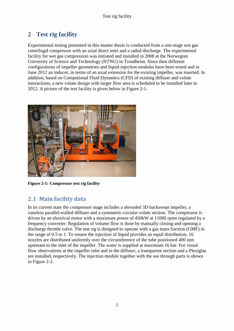
2 Test rig facility
Experimental testing presented in this master thesis is conducted from a one-stage wet gas
centrifugal compressor with an axial direct inlet and a radial discharge. The experimental
facility for wet gas compression was initiated and installed in 2008 at the Norwegian
University of Science and Technology (NTNU) in Trondheim. Since then different
configurations of impeller geometries and liquid injection modules have been tested and in
June 2012 an inducer, in terms of an axial extension for the existing impeller, was inserted. In
addition, based on Computional Fluid Dynamics (CFD) of existing diffuser and volute
interactions, a new volute design with larger flow area is scheduled to be installed later in
2012. A picture of the test facility is given below in Figure 2-1.
Figure 2-1: Compressor test rig facility
2.1 Main facility data
In its current state the compressor stage includes a shrouded 3D backswept impeller, a
vaneless parallel-walled diffuser and a symmetric-circular volute section. The compressor is
driven by an electrical motor with a maximum power of 450kW at 11000 rpms regulated by a
frequency converter. Regulation of volume flow is done by manually closing and opening a
discharge throttle valve. The test rig is designed to operate with a gas mass fraction (GMF) in
the range of 0.5 to 1. To ensure the injection of liquid provides an equal distribution, 16
nozzles are distributed uniformly over the circumference of the tube positioned 400 mm
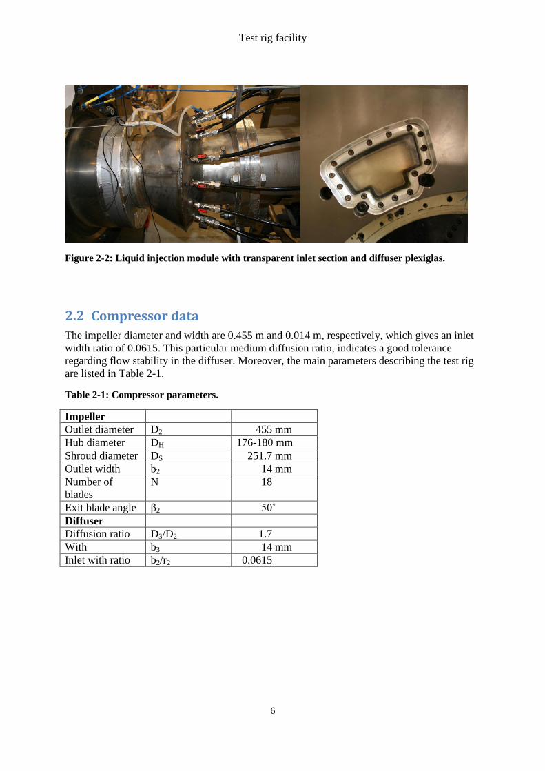
upstream to the inlet of the impeller. The water is supplied at maximum 16 bar. For visual
flow observations at the impeller inlet and in the diffuser, a transparent section and a Plexiglas
are installed, respectively. The injection module together with the see through parts is shown
in Figure 2-2.
Test rig facility
6
Figure 2-2: Liquid injection module with transparent inlet section and diffuser plexiglas.
2.2 Compressor data
The impeller diameter and width are 0.455 m and 0.014 m, respectively, which gives an inlet
width ratio of 0.0615. This particular medium diffusion ratio, indicates a good tolerance
regarding flow stability in the diffuser. Moreover, the main parameters describing the test rig
are listed in Table 2-1.
Table 2-1: Compressor parameters.
Impeller
Outlet diameter D2 455 mm
Hub diameter DH 176-180 mm
Shroud diameter DS 251.7 mm
Outlet width b2 14 mm
Number of
blades
N 18
Exit blade angle β2 50˚
Diffuser
Diffusion ratio D3/D2 1.7
With b3 14 mm
Inlet with ratio b2/r2 0.0615
Test rig facility
7
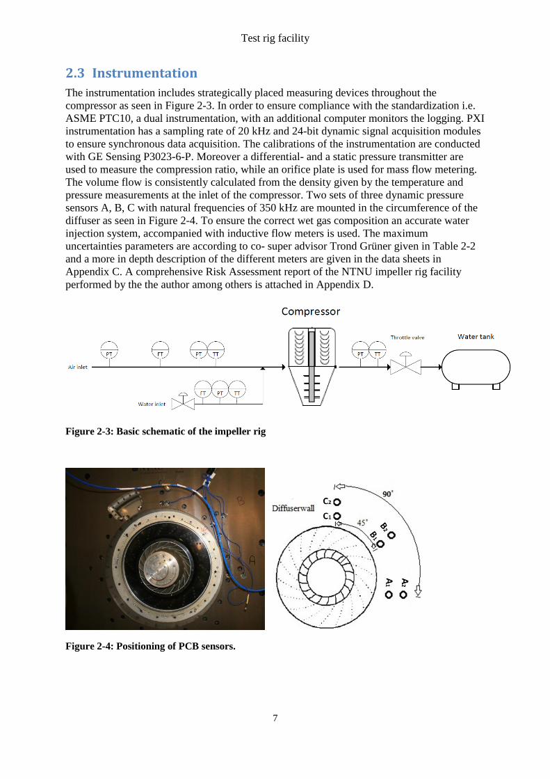
2.3 Instrumentation
The instrumentation includes strategically placed measuring devices throughout the
compressor as seen in Figure 2-3. In order to ensure compliance with the standardization i.e.
ASME PTC10, a dual instrumentation, with an additional computer monitors the logging. PXI
instrumentation has a sampling rate of 20 kHz and 24-bit dynamic signal acquisition modules
to ensure synchronous data acquisition. The calibrations of the instrumentation are conducted
with GE Sensing P3023-6-P. Moreover a differential- and a static pressure transmitter are
used to measure the compression ratio, while an orifice plate is used for mass flow metering.
The volume flow is consistently calculated from the density given by the temperature and
pressure measurements at the inlet of the compressor. Two sets of three dynamic pressure
sensors A, B, C with natural frequencies of 350 kHz are mounted in the circumference of the
diffuser as seen in Figure 2-4. To ensure the correct wet gas composition an accurate water
injection system, accompanied with inductive flow meters is used. The maximum
uncertainties parameters are according to co- super advisor Trond Grüner given in Table 2-2
and a more in depth description of the different meters are given in the data sheets in
Appendix C. A comprehensive Risk Assessment report of the NTNU impeller rig facility
performed by the the author among others is attached in Appendix D.
Figure 2-3: Basic schematic of the impeller rig
Figure 2-4: Positioning of PCB sensors.
Test rig facility
8
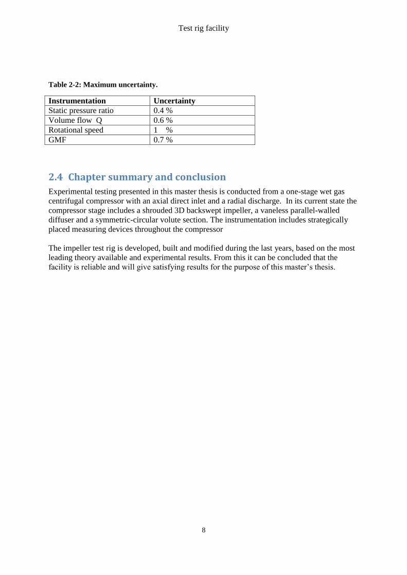
Table 2-2: Maximum uncertainty.
Instrumentation Uncertainty
Static pressure ratio 0.4 %
Volume flow Q 0.6 %
Rotational speed 1 %
GMF 0.7 %
2.4 Chapter summary and conclusion
Experimental testing presented in this master thesis is conducted from a one-stage wet gas
centrifugal compressor with an axial direct inlet and a radial discharge. In its current state the
compressor stage includes a shrouded 3D backswept impeller, a vaneless parallel-walled
diffuser and a symmetric-circular volute section. The instrumentation includes strategically
placed measuring devices throughout the compressor
The impeller test rig is developed, built and modified during the last years, based on the most
leading theory available and experimental results. From this it can be concluded that the
facility is reliable and will give satisfying results for the purpose of this master’s thesis.
Multiphase flow
9
3 Multiphase flow
Explanations and equations in this chapter have different relevancy to the master thesis, but
will give a more thorough fundament for understanding the multiphase effects on the flow.
3.1 Multiphase fundamentals
Multiphase flow for wet gas compression is defined from an industrial point of view as a gas
containing maximum 5% liquid on volume basis, i.e. gas volume fraction (GVF) between
0.95 and 1. However, the gas mass fraction (GMF) can at the same time be less than 0.5 for
low pressure ratios verified by Grüner and Bakken [3] among others through experiments.
Unfortunately most available work is based on gas containing less than 0.95 on a gas volume
fraction (GVF), which makes it somewhat difficult to compare previous work with this master
thesis. However, in lack of better experiments, they will, to some extent, be used for
comparison. Equations for GVF and GMF are:
g
g l
QGVF
Q Q
Equation 3-1
g
g l
mGMF
m m
Equation 3-2
Normally the GVF parameter is the most preferred one for wet gas fluid mechanics
comparison because its properties reflecting geometrics of the fluid mechanic conditions.
Nonetheless, the GMF parameter is preferred in application in thermo-analysis as it has
proven to be the best parameter in terms of wet gas at low pressure conditions.
The ability of liquid droplets to respond to the gas flow i.e. indicates the possibilities for
phase separation depends on the ratio given by Equation 3-3.
* g
l
Equation 3-3
This simplifies the complex multiphase model into single phase behavior with a consistent
density given by:
(1 )h g l
Equation 3-4
Furthermore, the velocity regarding the multiphase components are denoted VSG and VSL i.e.
superficial velocity meaning the single- phase velocity based on mass flow and channel cross-
section area. The superficial velocities given in Equation 3-5 and Equation 3-6 are particularly
important parameters in order to determine in which flow regime a current flow is categorized
as.
g
SG
g CR
mV
A
Equation 3-5
Multiphase flow
10
lSL
l CR
mV
A
Equation 3-6
With that in hand a new expression for GMF is obtained, showing how the gas mass fraction
term incorporates the phase density difference by the use of Equation 3-2 and Equation 3-6.
*
*
SG
SG SL
VGMF
V V
Equation 3-7
which can also be written
*/
g
g l
QGVF
Q Q
Equation 3-8
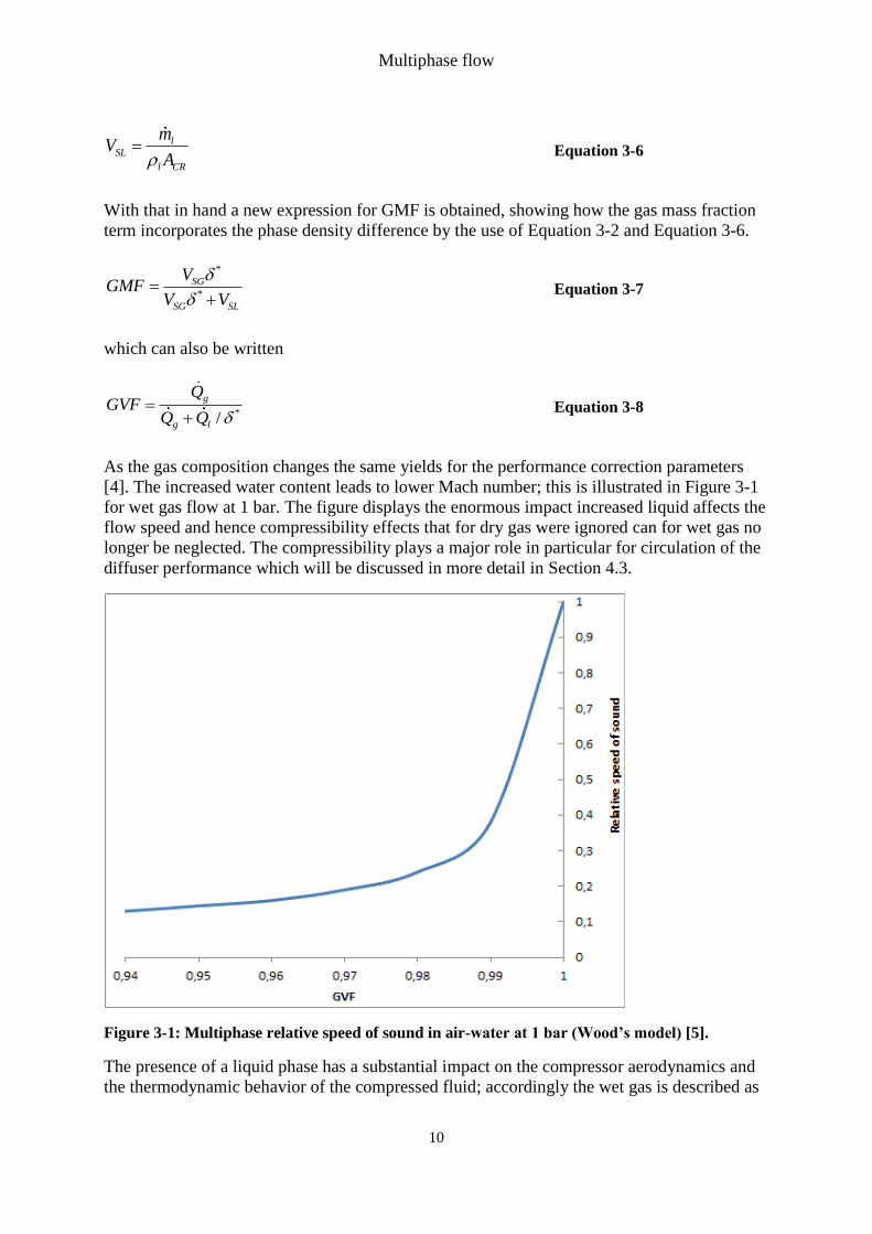
As the gas composition changes the same yields for the performance correction parameters
[4]. The increased water content leads to lower Mach number; this is illustrated in Figure 3-1
for wet gas flow at 1 bar. The figure displays the enormous impact increased liquid affects the
flow speed and hence compressibility effects that for dry gas were ignored can for wet gas no
longer be neglected. The compressibility plays a major role in particular for circulation of the
diffuser performance which will be discussed in more detail in Section 4.3.
Figure 3-1: Multiphase relative speed of sound in air-water at 1 bar (Wood’s model) [5].
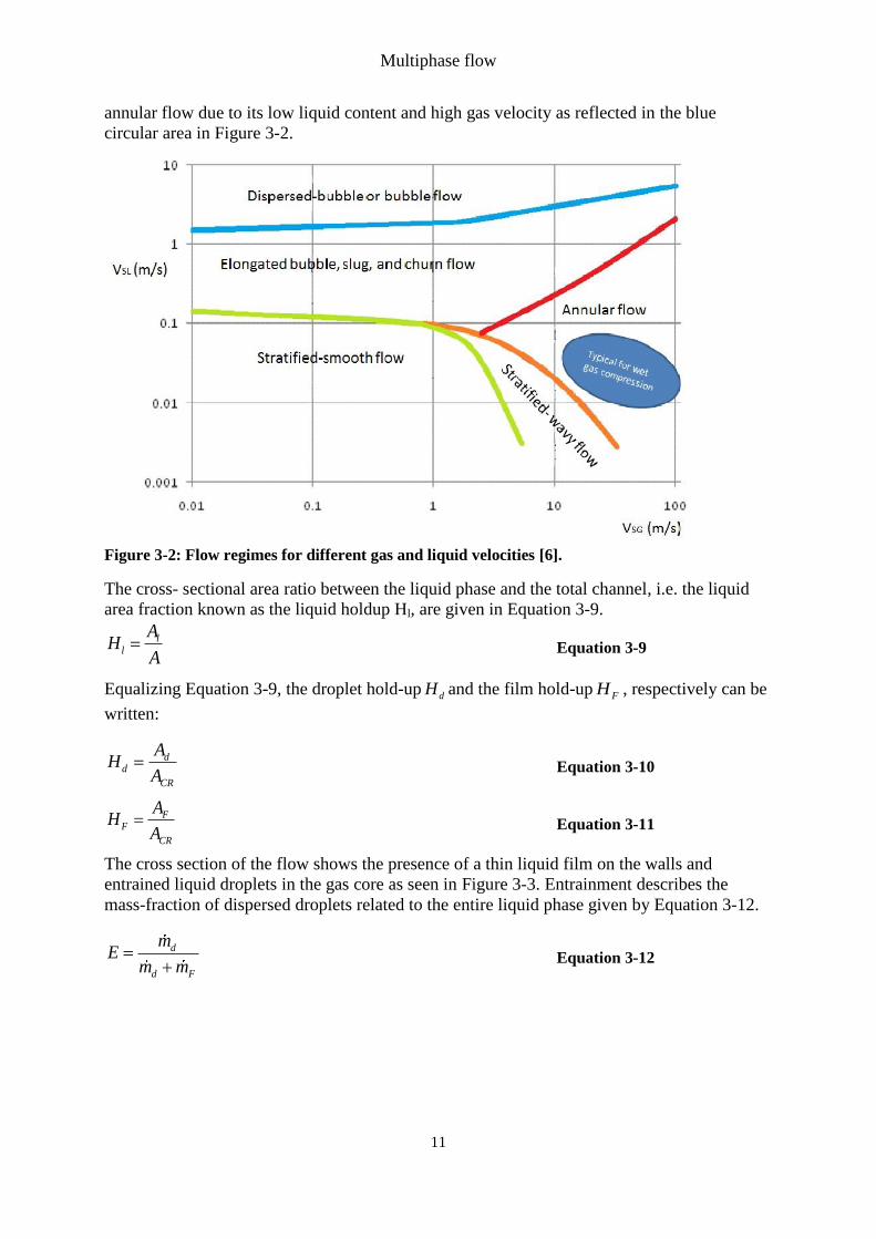
The presence of a liquid phase has a substantial impact on the compressor aerodynamics and
the thermodynamic behavior of the compressed fluid; accordingly the wet gas is described as
Multiphase flow
11
annular flow due to its low liquid content and high gas velocity as reflected in the blue
circular area in Figure 3-2.
Figure 3-2: Flow regimes for different gas and liquid velocities [6].
The cross- sectional area ratio between the liquid phase and the total channel, i.e. the liquid
area fraction known as the liquid holdup Hl, are given in Equation 3-9.
ll
AH
A
Equation 3-9
Equalizing Equation 3-9, the droplet hold-up dH and the film hold-up FH , respectively can be
written:
dd
CR
AH
A
Equation 3-10
FF
CR
AH
A
Equation 3-11
The cross section of the flow shows the presence of a thin liquid film on the walls and
entrained liquid droplets in the gas core as seen in Figure 3-3. Entrainment describes the
mass-fraction of dispersed droplets related to the entire liquid phase given by Equation 3-12.
d
d F
mE
m m
Equation 3-12

Multiphase flow
12
Figure 3-3: Sketch of annular flow.
Regarding gas compression, wet gas that passes the impeller inlet is characterized by
dispersed droplets in the core and as dense droplet spray in the core that furthermore prevails
through the impeller and the diffuser. The interaction between the phases contributes to
multiphase effects not present in single phase flow and it is therefore of high value to identify
the liquid distribution in the flow. The interfacial effects between the two phases results in
energy, mass and momentum transfer which alter the flow characteristics significantly from
single phase flow. Consequently wet gas flow have complicated characteristics given by the
interactions and relative movement between the phases[4].
The liquid film in an annular flow will not be symmetrical. Due to gravity the liquid film will
always be in the lower part of a tube channel to be thicker than the upper section. The average
film thickness around the pipe can be expressed as[7]:
2
4
top side bottom
Equation 3-13
Hence, an approximation to a film thickness correlation is given as:
3
412,5 RegasD
Equation 3-14
where the liquid flow is completely ignored, regardless it gives an good accuracy according to
Schubring [7] within a Mean Absolute Error (MAE) of 11%. The MAE relation is given in
Equation 3-15.
, exp,
1 exp,
1100%
ncorr i i
i i
x xMAE
n x
Equation 3-15
Furthermore Schubring findings suggest that the base film thickness is inversely related to gas
flow and increases with increasing liquid flow, due to increased shear stress. At high gas flow
rates, the dependence of liquid flow becomes small. Asymmetry shows similar gross trends as
Multiphase flow
13
average base film thickness, with an dominant inverse gas flow rate effect and small liquid
flow rate effect that is most significant both increase with increasing diameter, but the
dependencies are less than linear [7].
3.2 Multiphase effects on the boundary layer
This section gives a brief introduction to the development of boundary layer and the
multiphase effects. The latter are important in order to, among other things, explain the
occurrence of compressor instabilities that is caused by boundary layer separation. However,
aerodynamic instabilities and boundary layer separation are treated in more detail in Chapter5.
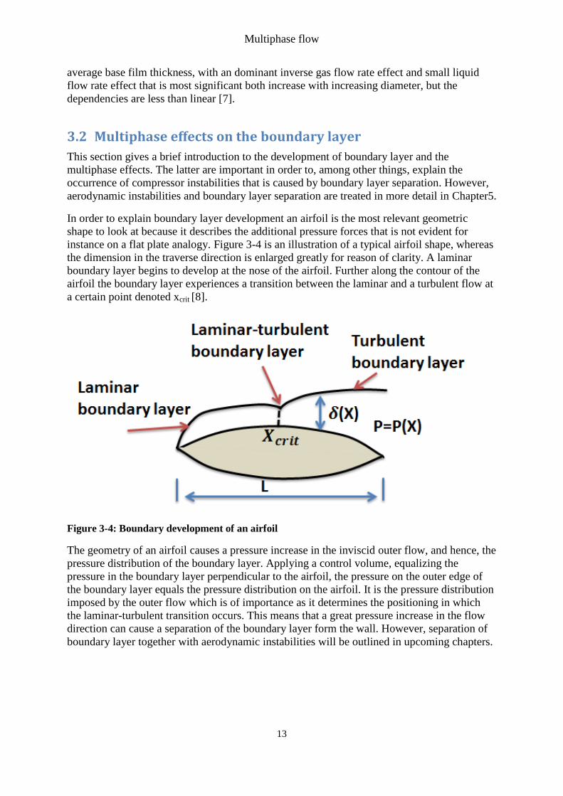
In order to explain boundary layer development an airfoil is the most relevant geometric
shape to look at because it describes the additional pressure forces that is not evident for
instance on a flat plate analogy. Figure 3-4 is an illustration of a typical airfoil shape, whereas
the dimension in the traverse direction is enlarged greatly for reason of clarity. A laminar
boundary layer begins to develop at the nose of the airfoil. Further along the contour of the
airfoil the boundary layer experiences a transition between the laminar and a turbulent flow at
a certain point denoted xcrit [8].
Figure 3-4: Boundary development of an airfoil
The geometry of an airfoil causes a pressure increase in the inviscid outer flow, and hence, the
pressure distribution of the boundary layer. Applying a control volume, equalizing the
pressure in the boundary layer perpendicular to the airfoil, the pressure on the outer edge of
the boundary layer equals the pressure distribution on the airfoil. It is the pressure distribution
imposed by the outer flow which is of importance as it determines the positioning in which
the laminar-turbulent transition occurs. This means that a great pressure increase in the flow
direction can cause a separation of the boundary layer form the wall. However, separation of
boundary layer together with aerodynamic instabilities will be outlined in upcoming chapters.

Multiphase flow
14
3.3 Chapter summary and conclusion
Multiphase flow for wet gas compression contains maximum 5% liquid on volume basis, i.e.
gas volume fraction (GVF) between 0.95 and 1. However, the gas mass fraction (GMF) can
be less than 0.5.The presence of a liquid phase has a substantial impact on the compressor
aerodynamics and the thermodynamic behavior of the compressed fluid; accordingly the wet
gas is described as annular flow due to its low liquid content and high gas velocity. Wet gas
that passes the impeller inlet is characterized by dispersed droplets in the core and as dense
droplet spray in the core that furthermore prevails through the impeller and the diffuser.
Aerodynamic in centrifugal compressor
15
4 Aerodynamic in centrifugal compressor
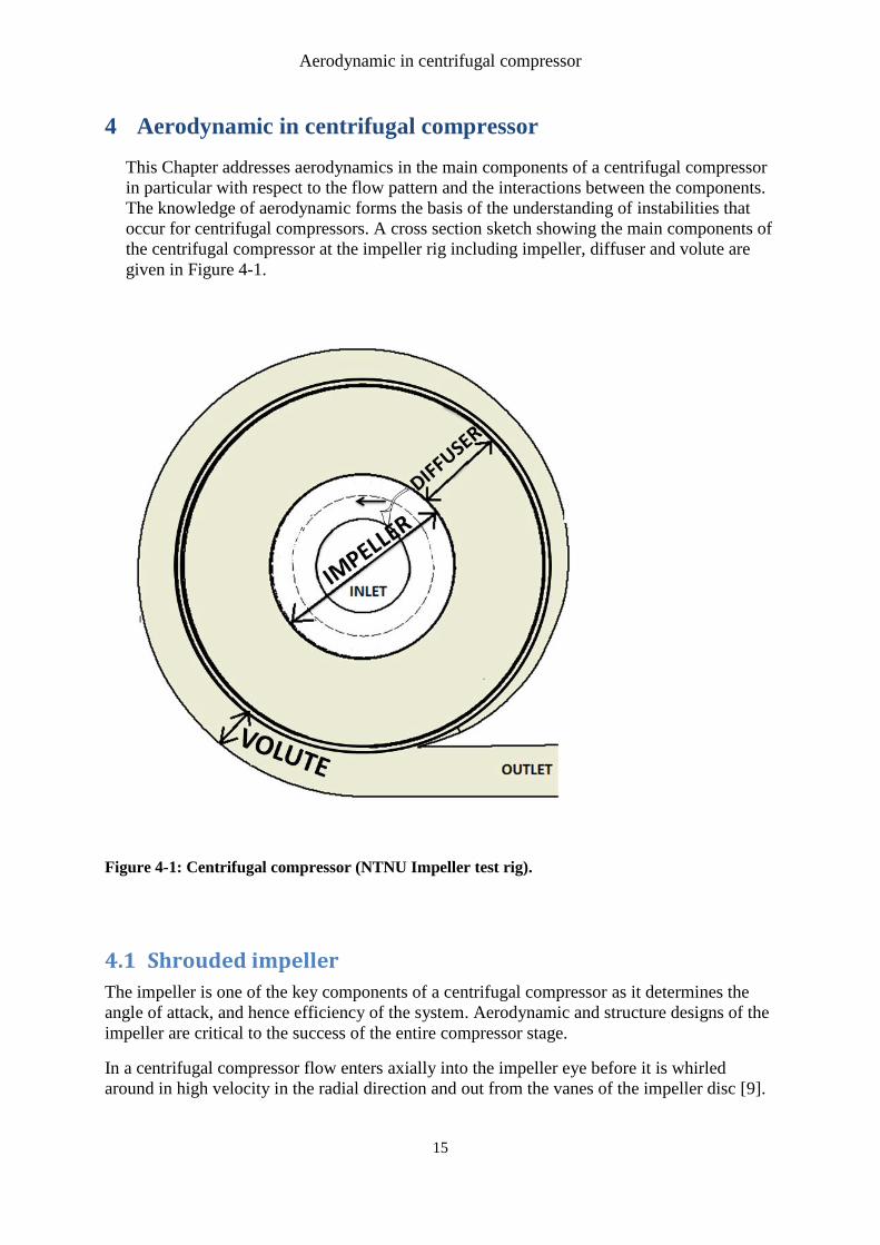
This Chapter addresses aerodynamics in the main components of a centrifugal compressor
in particular with respect to the flow pattern and the interactions between the components.
The knowledge of aerodynamic forms the basis of the understanding of instabilities that
occur for centrifugal compressors. A cross section sketch showing the main components of
the centrifugal compressor at the impeller rig including impeller, diffuser and volute are
given in Figure 4-1.
Figure 4-1: Centrifugal compressor (NTNU Impeller test rig).
4.1 Shrouded impeller
The impeller is one of the key components of a centrifugal compressor as it determines the
angle of attack, and hence efficiency of the system. Aerodynamic and structure designs of the
impeller are critical to the success of the entire compressor stage.
In a centrifugal compressor flow enters axially into the impeller eye before it is whirled
around in high velocity in the radial direction and out from the vanes of the impeller disc [9].
Aerodynamic in centrifugal compressor
16
The static pressure of the air increases from the eye to the tip of the impeller, in order to
accelerate the flow to obtain the necessary pressure head.
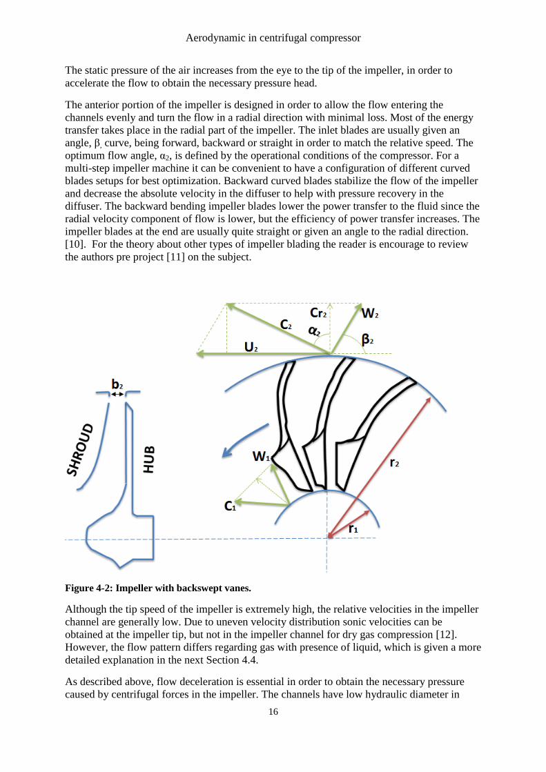
The anterior portion of the impeller is designed in order to allow the flow entering the
channels evenly and turn the flow in a radial direction with minimal loss. Most of the energy
transfer takes place in the radial part of the impeller. The inlet blades are usually given an
angle, β, curve, being forward, backward or straight in order to match the relative speed. The
optimum flow angle, α2, is defined by the operational conditions of the compressor. For a
multi-step impeller machine it can be convenient to have a configuration of different curved
blades setups for best optimization. Backward curved blades stabilize the flow of the impeller
and decrease the absolute velocity in the diffuser to help with pressure recovery in the
diffuser. The backward bending impeller blades lower the power transfer to the fluid since the
radial velocity component of flow is lower, but the efficiency of power transfer increases. The
impeller blades at the end are usually quite straight or given an angle to the radial direction.
[10]. For the theory about other types of impeller blading the reader is encourage to review
the authors pre project [11] on the subject.
Figure 4-2: Impeller with backswept vanes.
Although the tip speed of the impeller is extremely high, the relative velocities in the impeller
channel are generally low. Due to uneven velocity distribution sonic velocities can be
obtained at the impeller tip, but not in the impeller channel for dry gas compression [12].
However, the flow pattern differs regarding gas with presence of liquid, which is given a more
detailed explanation in the next Section 4.4.
As described above, flow deceleration is essential in order to obtain the necessary pressure
caused by centrifugal forces in the impeller. The channels have low hydraulic diameter in
Aerodynamic in centrifugal compressor
17
relation to axial compressors and are therefore subject to greater friction at the channel walls.
An uneven velocity distribution along the impellers causes an uneven pressure distribution
and, consequently a temporal variation in both pressure and velocity of the flow entering the
diffuser [12].
4.1.1 Impeller flow patterns
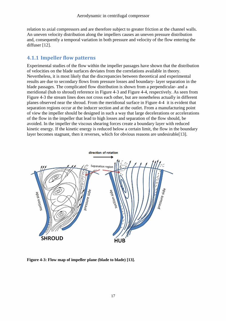
Experimental studies of the flow within the impeller passages have shown that the distribution
of velocities on the blade surfaces deviates from the correlations available in theory.
Nevertheless, it is most likely that the discrepancies between theoretical and experimental
results are due to secondary flows from pressure losses and boundary- layer separation in the
blade passages. The complicated flow distribution is shown from a perpendicular- and a
meridional (hub to shroud) reference in Figure 4-3 and Figure 4-4, respectively. As seen from
Figure 4-3 the stream lines does not cross each other, but are nonetheless actually in different
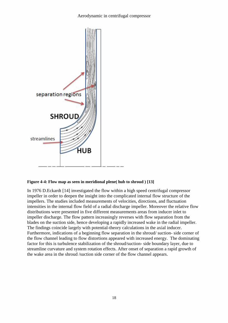
planes observed near the shroud. From the meridional surface in Figure 4-4 it is evident that
separation regions occur at the inducer section and at the outlet. From a manufacturing point
of view the impeller should be designed in such a way that large decelerations or accelerations
of the flow in the impeller that lead to high losses and separation of the flow should, be
avoided. In the impeller the viscous shearing forces create a boundary layer with reduced
kinetic energy. If the kinetic energy is reduced below a certain limit, the flow in the boundary
layer becomes stagnant, then it reverses, which for obvious reasons are undesirable[13].
Figure 4-3: Flow map of impeller plane (blade to blade) [13].
Aerodynamic in centrifugal compressor
18
Figure 4-4: Flow map as seen in meridional plene( hub to shroud ) [13]
In 1976 D.Eckardt [14] investigated the flow within a high speed centrifugal compressor
impeller in order to deepen the insight into the complicated internal flow structure of the
impellers. The studies included measurements of velocities, directions, and fluctuation
intensities in the internal flow field of a radial discharge impeller. Moreover the relative flow
distributions were presented in five different measurements areas from inducer inlet to
impeller discharge. The flow pattern increasingly reverses with flow separation from the
blades on the suction side, hence developing a rapidly increased wake in the radial impeller.
The findings coincide largely with potential-theory calculations in the axial inducer.
Furthermore, indications of a beginning flow separation in the shroud/ suction- side corner of
the flow channel leading to flow distortions appeared with increased energy. The dominating
factor for this is turbulence stabilization of the shroud/suction- side boundary layer, due to
streamline curvature and system rotation effects. After onset of separation a rapid growth of
the wake area in the shroud /suction side corner of the flow channel appears.
Aerodynamic in centrifugal compressor
19
4.2 Impeller and diffuser interactions
The flow on the outlet of the impeller is not completely guided by the blades. This section
will outline the theory describing factors affecting the outlet flow of the impeller as it is not
solely guided by the blades. In the case of an impeller with backswept blades the effective
fluid outlet angle does not equal the blade outlet angle. For this deviation the slip factor given
in Equation 4-1 is used.
2
2
C
C
Equation 4-1
Where CƟ2 is the tangential component of the absolute exit velocity with a finite number of
blades and and CƟ2∞ is the tangential component of the absolute exit velocity given infinite
number of blades.
A definite cause of the slip phenomena that occurs within an impeller is not known,
nevertheless the coriolis circulation, the theory with boundary layer development among other
factors contributes to underline the explanation of why the flow is changed. The combined
forces from pressure gradient between the walls of two adjacent blades, the Coriolis forces,
the centrifugal forces, and the fluid causes a fluid movement from one wall to the other and
vice versa. Consequently this movement sets up circulation within the passage resulting with
a net change in the exit angle at the impeller exit.
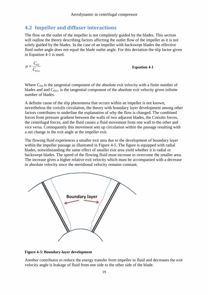
The flowing fluid experiences a smaller exit area due to the development of boundary layer
within the impeller passage as illustrated in Figure 4-5. The figure is equipped with radial
blades, notwithstanding the same effect of smaller exit area yield whether it is radial or
backswept blades. The speed of the flowing fluid must increase to overcome the smaller area.
The increase gives a higher relative exit velocity which must be accompanied with a decrease
in absolute velocity since the meridional velocity remains constant.
Figure 4-5: Boundary-layer development
Another contributor to reduce the energy transfer from impeller to fluid and decreases the exit
velocity angle is leakage of fluid from one side to the other side of the blade.
Aerodynamic in centrifugal compressor
20
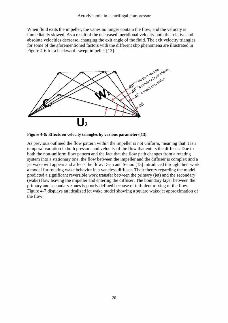
When fluid exits the impeller, the vanes no longer contain the flow, and the velocity is
immediately slowed. As a result of the decreased meridional velocity both the relative and
absolute velocities decrease, changing the exit angle of the fluid. The exit velocity triangles
for some of the aforementioned factors with the different slip phenomena are illustrated in
Figure 4-6 for a backward- swept impeller [13].
Figure 4-6: Effects on velocity triangles by various parameters[13].
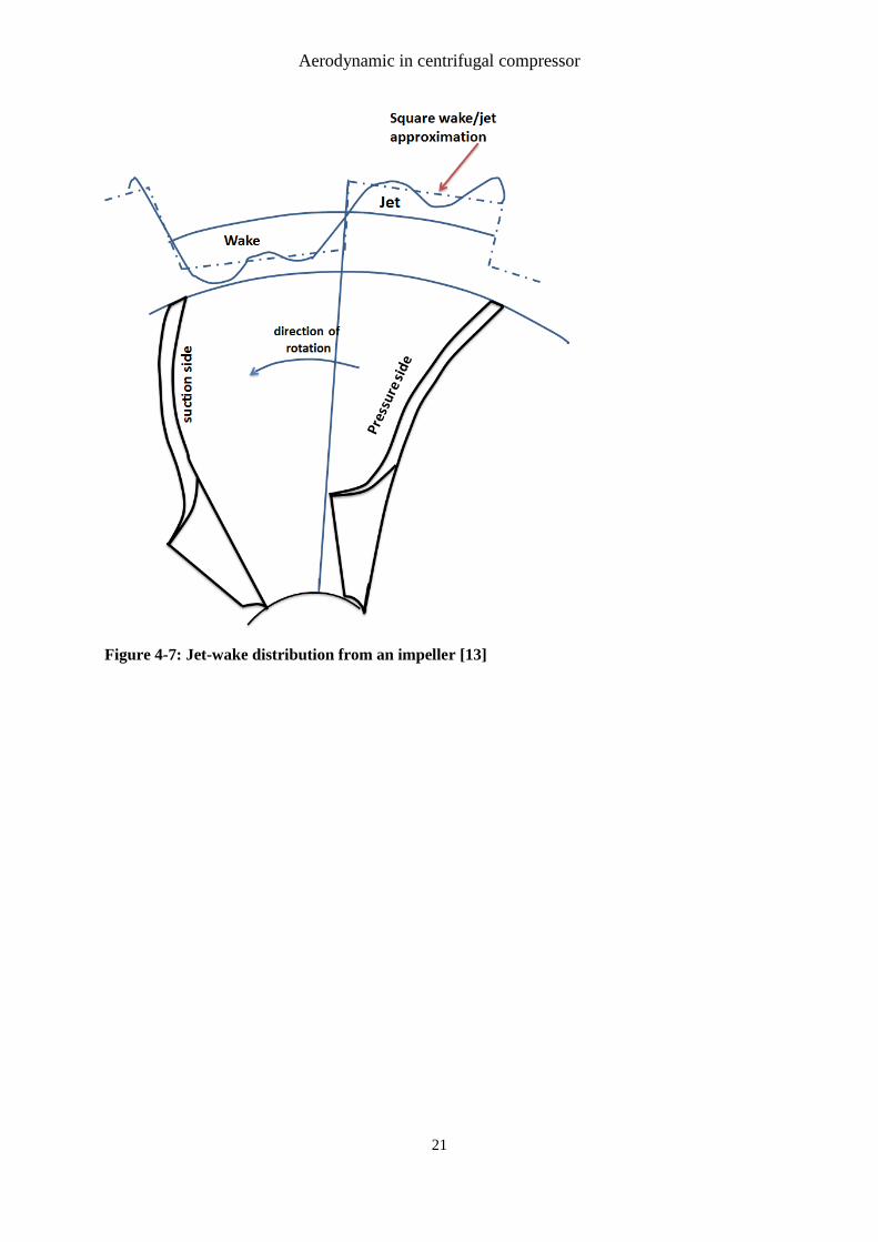
As previous outlined the flow pattern within the impeller is not uniform, meaning that it is a
temporal variation in both pressure and velocity of the flow that enters the diffuser. Due to
both the non-uniform flow pattern and the fact that the flow path changes from a rotating
system into a stationary one, the flow between the impeller and the diffuser is complex and a
jet wake will appear and affects the flow. Dean and Senoo [15] introduced through their work
a model for rotating wake behavior in a vaneless diffuser. Their theory regarding the model
predicted a significant reversible work transfer between the primary (jet) and the secondary
(wake) flow leaving the impeller and entering the diffuser. The boundary layer between the
primary and secondary zones is poorly defined because of turbulent mixing of the flow.
Figure 4-7 displays an idealized jet wake model showing a square wake/jet approximation of
the flow.
Aerodynamic in centrifugal compressor
21
Figure 4-7: Jet-wake distribution from an impeller [13]
Aerodynamic in centrifugal compressor
22
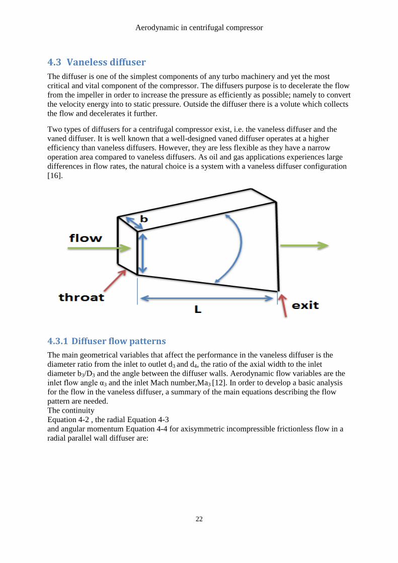
4.3 Vaneless diffuser
The diffuser is one of the simplest components of any turbo machinery and yet the most
critical and vital component of the compressor. The diffusers purpose is to decelerate the flow
from the impeller in order to increase the pressure as efficiently as possible; namely to convert
the velocity energy into to static pressure. Outside the diffuser there is a volute which collects
the flow and decelerates it further.
Two types of diffusers for a centrifugal compressor exist, i.e. the vaneless diffuser and the
vaned diffuser. It is well known that a well-designed vaned diffuser operates at a higher
efficiency than vaneless diffusers. However, they are less flexible as they have a narrow
operation area compared to vaneless diffusers. As oil and gas applications experiences large
differences in flow rates, the natural choice is a system with a vaneless diffuser configuration
[16].
4.3.1 Diffuser flow patterns
The main geometrical variables that affect the performance in the vaneless diffuser is the
diameter ratio from the inlet to outlet d3 and d4, the ratio of the axial width to the inlet
diameter b3/D3 and the angle between the diffuser walls. Aerodynamic flow variables are the
inlet flow angle α3 and the inlet Mach number,Ma3 [12]. In order to develop a basic analysis
for the flow in the vaneless diffuser, a summary of the main equations describing the flow
pattern are needed.
The continuity
Equation 4-2 , the radial Equation 4-3
and angular momentum Equation 4-4 for axisymmetric incompressible frictionless flow in a
radial parallel wall diffuser are:
Aerodynamic in centrifugal compressor
23
0
1( ) 0rp rv
r r
Equation 4-2
2
0
1rr
vv pv
r r r
Equation 4-3
0rr
v v vv
r r
Equation 4-4
Hence the flow is assumed to be steady for the simplified analysis and the tangential pressure
gradient is assumed to be zero. An integration of the continuity and the angular momentum
equation gives Equation 4-5 and Equation 4-6.
3 3r rrv r v
Equation 4-5
3 3rv r v
Equation 4-6
by combining Equation 4-4, Equation 4-5 and Equation 4-6 the equation becomes:
231
2
0 3
(1 ( ) )1
2
rp p
rv
2 2 2
3 3 3rv v v
Equation 4-7
In an incompressible flow, both the radial and the tangential velocity components decrease
with increased radius. Thus from continuity and conservation of angular momentum, both
velocity components are reduced in the vaneless diffuser due to the increase in the radius. A
streamline for an incompressible flow is given by Equation 4-8
1 rvdr
r d v
Equation 4-8
Assumed steady, frictionless, axisymmetric flow i.e. by using Equation 4-4 and Equation 4-5,
the equation becomes:
3
3
1 rvdr
r d v
Equation 4-9
Moreover, by integrating Equation 4-8 from the diffuser inlet yields:
3
3
( )ln
tan( )L
r
r
1 3
3
tan ( )L
r
v
v
Equation 4-10
which is an equation of a logarithmic spiral, which forms an angle, αL ,with any radial line,
where, αL, is termed the logarithmic spiral angle. Thus, the incompressible flow in a parallel
wall radial diffuser follows logarithmic spiral streamlines [17].
Aerodynamic in centrifugal compressor
24
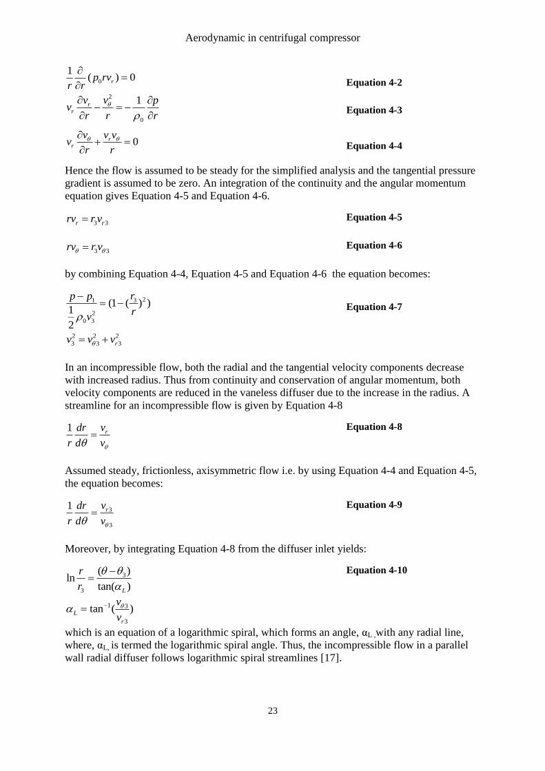
Regardless of the simple design of a vaneless diffuser the flow theory is rather complicated
which is due to the non-uniform flow discharged from the impeller. In addition to non-
uniform flow, the logarithmic flow lines, that is long flow paths through the diffuser, prevails
viscous shear forces between the fluid and the walls resulting in several secondary flows. In
order to decrease the tangential deflection, and hence the flow path through the diffuser, the
diffuser width can be reduced with increasing radius. This will cause a small decrease in
radial velocity compared to parallel walls, while the tangential velocity will decrease with
decreased diffuser width. A decrease in the axial diffuser width, will decrease the radial
velocity due to continuity, however, this will have little effect on the tangential speed [18].
Compressibility plays a major role in the calculation of the diffuser performance. Since the
retarded fluid through the diffuser increases the pressure and density. This increase in density
helps to slow the radial velocity further by increasing the radius. The tangential velocity is not
affected by this effect and thus has the real flow a greater tendency to bend in the tangential
direction than the radial [18]. The Figure 4-8 show a good flow path in the diffuser with the
radial, R and the tangential, T, component drawn in.
Figure 4-8: Tangential and radial direction in diffuser flow
Aerodynamic in centrifugal compressor
25
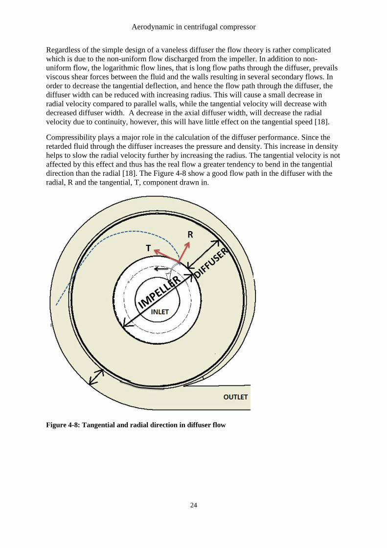
Figure 4-9: Diffuser performance with good performance.
Figure 4-10 : Actual measured boundary layer separation and poor performance.
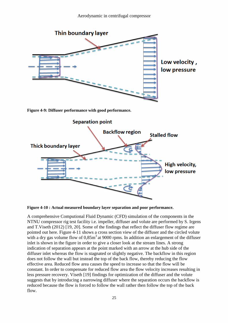
A comprehensive Computional Fluid Dynamic (CFD) simulation of the components in the
NTNU compressor rig test facility i.e. impeller, diffuser and volute are performed by S. Irgens
and T.Viseth (2012) [19, 20]. Some of the findings that reflect the diffuser flow regime are
pointed out here. Figure 4-11 shows a cross section view of the diffuser and the circled volute
with a dry gas volume flow of 0,85m3
at 9000 rpms. In addition an enlargement of the diffuser
inlet is shown in the figure in order to give a closer look at the stream lines. A strong
indication of separation appears at the point marked with an arrow at the hub side of the
diffuser inlet whereas the flow is stagnated or slightly negative. The backflow in this region
does not follow the wall but instead the top of the back flow, thereby reducing the flow
effective area. Reduced flow area causes the speed to increase so that the flow will be
constant. In order to compensate for reduced flow area the flow velocity increases resulting in
less pressure recovery. Viseth [19] findings for optimization of the diffuser and the volute
suggests that by introducing a narrowing diffuser where the separation occurs the backflow is
reduced because the flow is forced to follow the wall rather then follow the top of the back
flow.
Aerodynamic in centrifugal compressor
26
Figure 4-11:Cross section view of the diffuser and volute for 0.85m
3/s at 9000 rpm [19]
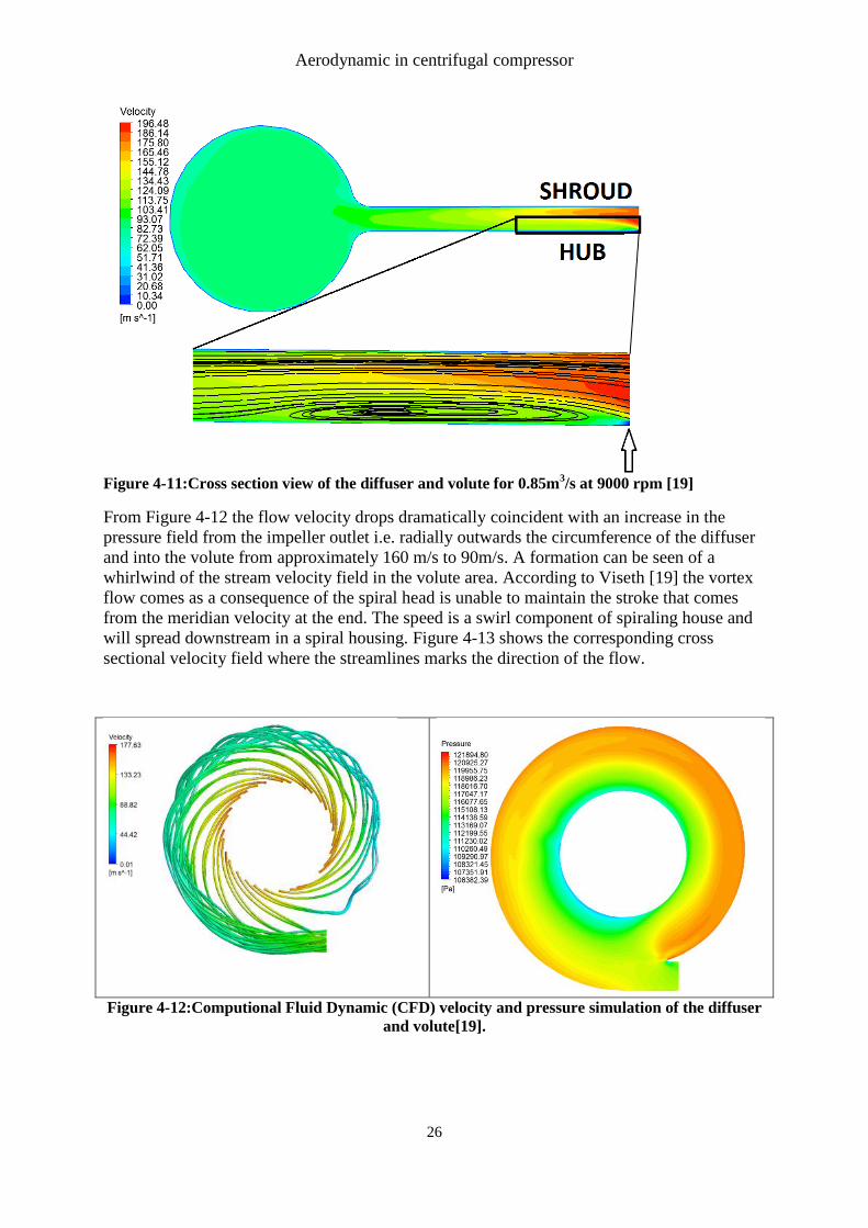
From Figure 4-12 the flow velocity drops dramatically coincident with an increase in the
pressure field from the impeller outlet i.e. radially outwards the circumference of the diffuser
and into the volute from approximately 160 m/s to 90m/s. A formation can be seen of a
whirlwind of the stream velocity field in the volute area. According to Viseth [19] the vortex
flow comes as a consequence of the spiral head is unable to maintain the stroke that comes
from the meridian velocity at the end. The speed is a swirl component of spiraling house and
will spread downstream in a spiral housing. Figure 4-13 shows the corresponding cross
sectional velocity field where the streamlines marks the direction of the flow.
Figure 4-12:Computional Fluid Dynamic (CFD) velocity and pressure simulation of the diffuser
and volute[19].
Aerodynamic in centrifugal compressor
27
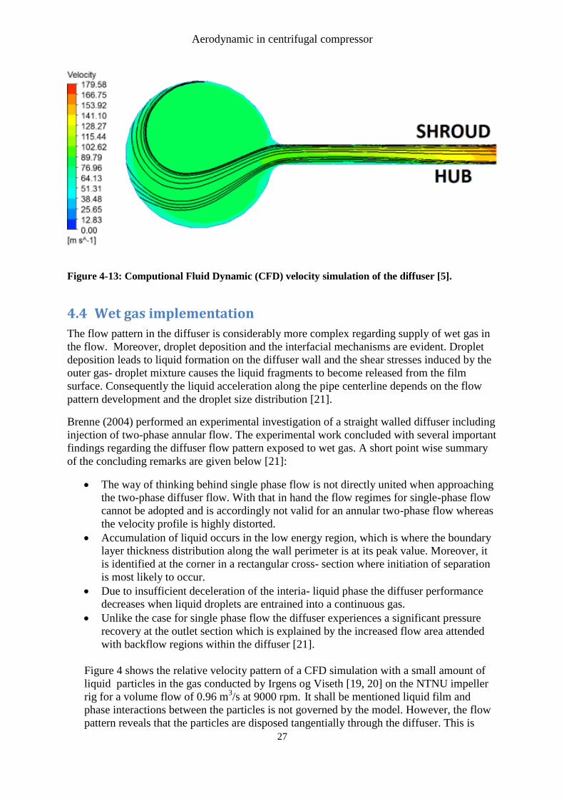
Figure 4-13: Computional Fluid Dynamic (CFD) velocity simulation of the diffuser [5].
4.4 Wet gas implementation
The flow pattern in the diffuser is considerably more complex regarding supply of wet gas in
the flow. Moreover, droplet deposition and the interfacial mechanisms are evident. Droplet
deposition leads to liquid formation on the diffuser wall and the shear stresses induced by the
outer gas- droplet mixture causes the liquid fragments to become released from the film
surface. Consequently the liquid acceleration along the pipe centerline depends on the flow
pattern development and the droplet size distribution [21].
Brenne (2004) performed an experimental investigation of a straight walled diffuser including
injection of two-phase annular flow. The experimental work concluded with several important
findings regarding the diffuser flow pattern exposed to wet gas. A short point wise summary
of the concluding remarks are given below [21]:
The way of thinking behind single phase flow is not directly united when approaching
the two-phase diffuser flow. With that in hand the flow regimes for single-phase flow
cannot be adopted and is accordingly not valid for an annular two-phase flow whereas
the velocity profile is highly distorted.
Accumulation of liquid occurs in the low energy region, which is where the boundary
layer thickness distribution along the wall perimeter is at its peak value. Moreover, it
is identified at the corner in a rectangular cross- section where initiation of separation
is most likely to occur.
Due to insufficient deceleration of the interia- liquid phase the diffuser performance
decreases when liquid droplets are entrained into a continuous gas.
Unlike the case for single phase flow the diffuser experiences a significant pressure
recovery at the outlet section which is explained by the increased flow area attended
with backflow regions within the diffuser [21].
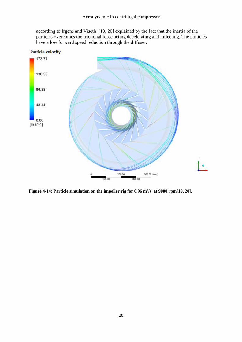
Figure 4 shows the relative velocity pattern of a CFD simulation with a small amount of
liquid particles in the gas conducted by Irgens og Viseth [19, 20] on the NTNU impeller
rig for a volume flow of 0.96 m3/s at 9000 rpm. It shall be mentioned liquid film and
phase interactions between the particles is not governed by the model. However, the flow
pattern reveals that the particles are disposed tangentially through the diffuser. This is
Aerodynamic in centrifugal compressor
28
according to Irgens and Viseth [19, 20] explained by the fact that the inertia of the
particles overcomes the frictional force acting decelerating and inflecting. The particles
have a low forward speed reduction through the diffuser.
Figure 4-14: Particle simulation on the impeller rig for 0.96 m3/s at 9000 rpm[19, 20].
Aerodynamic instabilities for dry gas
29
5 Aerodynamic instabilities for dry gas
Much of the text in this chapter are extracted and reproduced from the pre-project work by the
author [11] for practical considerations.
In compression systems, several types of instabilities can be present. Some of these are
combustion-, aero elastic -, and aerodynamic instabilities. The scope of this master thesis is
however limited to aerodynamic instabilities, with the respect of the surge phenomena for dry
and wet gas. As the theory of dry gas compression is well investigated and understood it is
chosen to limit the theory of aerodynamic instabilities in this chapter to dry gas. However, in
order to make it relevant for the investigation in this master thesis, it will be related to
compression of wet gas in Section 6.2. The section will also go into and discuss
implementation of wet gas in relation to dry gas.
5.1 Compressor instability for dry gas
According to Pampreen [22] the aerodynamic stability is in brief the compressors response to
disturbance that changes the operation point of the compressor. If the disturbance is
temporary which leads to a recurring operation point, the system is stable and otherwise it is
unstable. In other words, stability is the system’s ability to maintain or increase the outlet
pressure to a downstream reservoir, when decreasing the operation point of the compressor by
lowering the flow rate.
The performance of centrifugal compressors is highly influenced by aerodynamic instabilities
and it is important to distinguish between the different reasons to aerodynamic instabilities.
There are in general two types of instabilities that can be encountered in a compressor, known
as surge and stall. Surge and stall restricts the compressor performance (pressure rise) and
efficiency and can in outmost consequence cause great damage and possibly degradation of
the compressor. Surge and stall are therefore important instabilities to understand, whereas the
compressors performance is highly influenced by these mechanisms. While compressor
surging is in generally easy to understand, the concept of stall is more difficult to explain and
understand. Regardless of its complexity stall is an operation mode in which parts of the
compressor does not have an efficient energy transfer between the machine and fluid,
although the global compressor flow rate is mostly unaffected.
Instabilities are illustrated in Figure 5-1 which examines the case of a system consisting of a
compressor and a throttling valve downstream of the compressor. The figure can be used as a
tool to illustrate the unstable operating mode of a centrifugal compressor. The starting point is
at point A, which reflects the normal operation for the compressor. If the throttle valve is
closed, the volume flow through the compressor drops and the operating point moves from A
to B. The energy consumption will typically increase and losses are reduced resulting in a
higher pressure conditions. Somewhere between A and B the compressor will have a
maximum efficiency. The pressure ratio will still increase toward C by further choking
because power consumption increases more than the losses. Ultimately, power consumption
and losses will match and pressure ratio will reach its maximum. However, by closing the
valve further losses will exceed the power consumption and pressure ratio is reduced. In other
words, if you are at the operating point that yields the highest pressure conditions and throttle
the flow, the outlet pressure drop. The compressor will deliver a lower pressure compare to
the pressure which was delivered to the downstream reservoir at the previous operating point.
High pressure in the reservoir will lead to delays in the compressor; this is reflected in
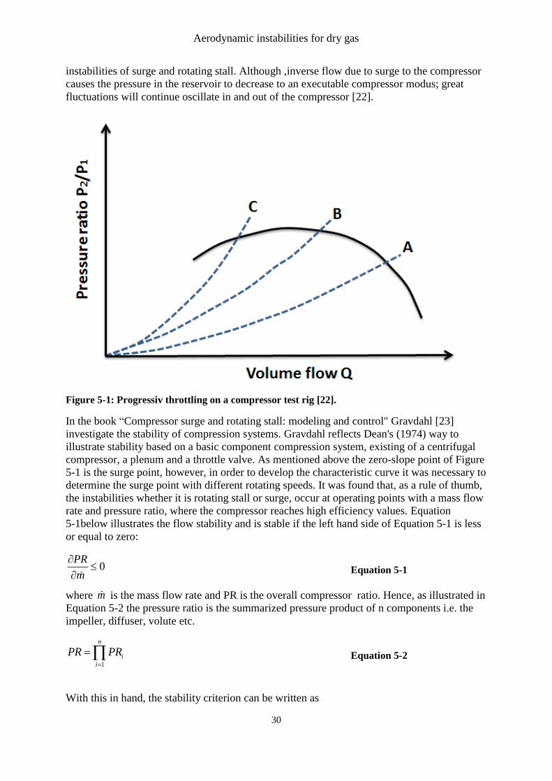
Aerodynamic instabilities for dry gas
30
instabilities of surge and rotating stall. Although ,inverse flow due to surge to the compressor
causes the pressure in the reservoir to decrease to an executable compressor modus; great
fluctuations will continue oscillate in and out of the compressor [22].
Figure 5-1: Progressiv throttling on a compressor test rig [22].
In the book “Compressor surge and rotating stall: modeling and control" Gravdahl [23]
investigate the stability of compression systems. Gravdahl reflects Dean's (1974) way to
illustrate stability based on a basic component compression system, existing of a centrifugal
compressor, a plenum and a throttle valve. As mentioned above the zero-slope point of Figure
5-1 is the surge point, however, in order to develop the characteristic curve it was necessary to
determine the surge point with different rotating speeds. It was found that, as a rule of thumb,
the instabilities whether it is rotating stall or surge, occur at operating points with a mass flow
rate and pressure ratio, where the compressor reaches high efficiency values. Equation
5-1below illustrates the flow stability and is stable if the left hand side of Equation 5-1 is less
or equal to zero:
0PR
m
Equation 5-1
where m is the mass flow rate and PR is the overall compressor ratio. Hence, as illustrated in
Equation 5-2 the pressure ratio is the summarized pressure product of n components i.e. the
impeller, diffuser, volute etc.
1
n
i
i
PR PR
Equation 5-2
With this in hand, the stability criterion can be written as
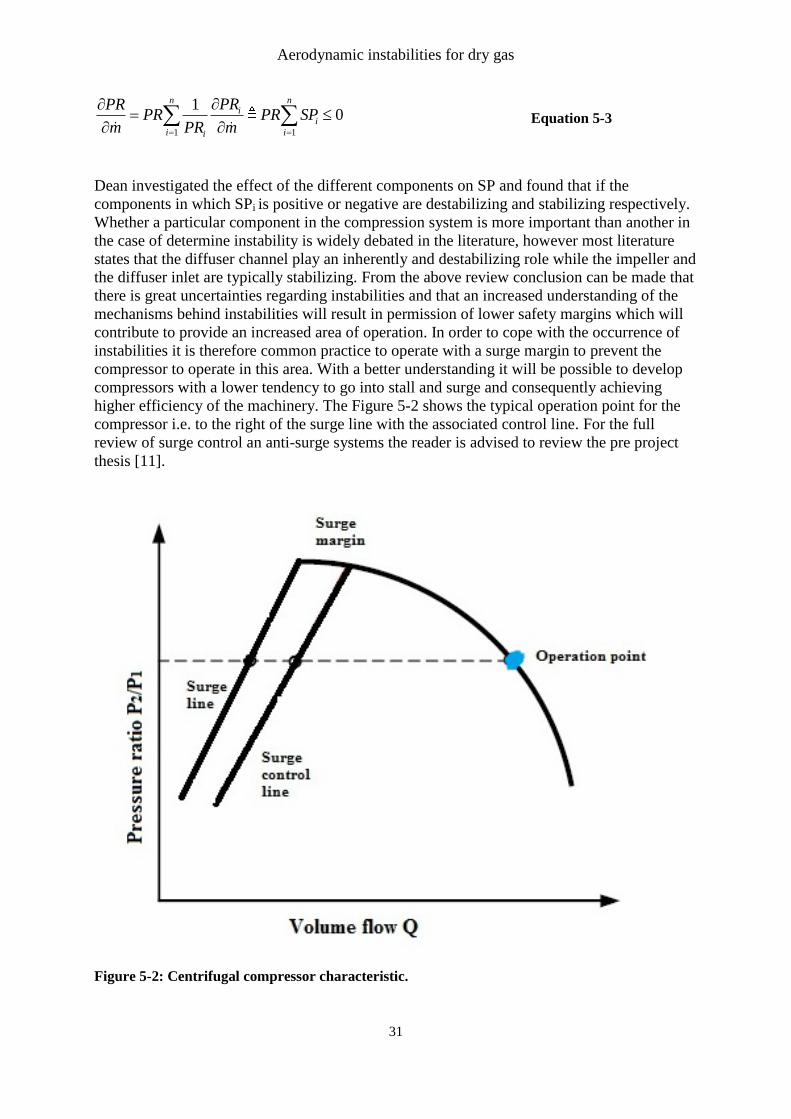
Aerodynamic instabilities for dry gas
31
1 1
10
n ni
i
i ii
PRPRPR PR SP
m PR m
Equation 5-3
Dean investigated the effect of the different components on SP and found that if the
components in which SPi is positive or negative are destabilizing and stabilizing respectively.
Whether a particular component in the compression system is more important than another in
the case of determine instability is widely debated in the literature, however most literature
states that the diffuser channel play an inherently and destabilizing role while the impeller and
the diffuser inlet are typically stabilizing. From the above review conclusion can be made that
there is great uncertainties regarding instabilities and that an increased understanding of the
mechanisms behind instabilities will result in permission of lower safety margins which will
contribute to provide an increased area of operation. In order to cope with the occurrence of
instabilities it is therefore common practice to operate with a surge margin to prevent the
compressor to operate in this area. With a better understanding it will be possible to develop
compressors with a lower tendency to go into stall and surge and consequently achieving
higher efficiency of the machinery. The Figure 5-2 shows the typical operation point for the
compressor i.e. to the right of the surge line with the associated control line. For the full
review of surge control an anti-surge systems the reader is advised to review the pre project
thesis [11].
Figure 5-2: Centrifugal compressor characteristic.
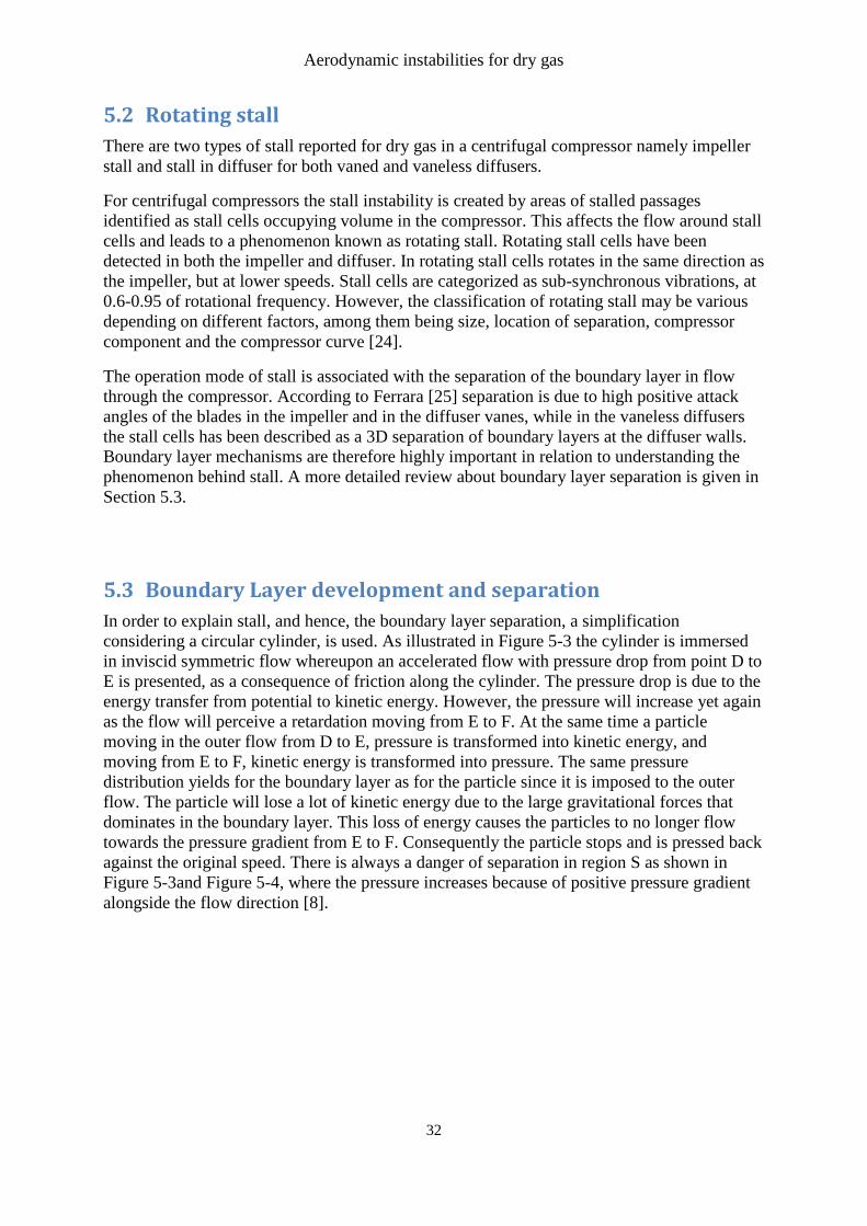
Aerodynamic instabilities for dry gas
32
5.2 Rotating stall
There are two types of stall reported for dry gas in a centrifugal compressor namely impeller
stall and stall in diffuser for both vaned and vaneless diffusers.
For centrifugal compressors the stall instability is created by areas of stalled passages
identified as stall cells occupying volume in the compressor. This affects the flow around stall
cells and leads to a phenomenon known as rotating stall. Rotating stall cells have been
detected in both the impeller and diffuser. In rotating stall cells rotates in the same direction as
the impeller, but at lower speeds. Stall cells are categorized as sub-synchronous vibrations, at
0.6-0.95 of rotational frequency. However, the classification of rotating stall may be various
depending on different factors, among them being size, location of separation, compressor
component and the compressor curve [24].
The operation mode of stall is associated with the separation of the boundary layer in flow
through the compressor. According to Ferrara [25] separation is due to high positive attack
angles of the blades in the impeller and in the diffuser vanes, while in the vaneless diffusers
the stall cells has been described as a 3D separation of boundary layers at the diffuser walls.
Boundary layer mechanisms are therefore highly important in relation to understanding the
phenomenon behind stall. A more detailed review about boundary layer separation is given in
Section 5.3.
5.3 Boundary Layer development and separation
In order to explain stall, and hence, the boundary layer separation, a simplification
considering a circular cylinder, is used. As illustrated in Figure 5-3 the cylinder is immersed
in inviscid symmetric flow whereupon an accelerated flow with pressure drop from point D to
E is presented, as a consequence of friction along the cylinder. The pressure drop is due to the
energy transfer from potential to kinetic energy. However, the pressure will increase yet again
as the flow will perceive a retardation moving from E to F. At the same time a particle
moving in the outer flow from D to E, pressure is transformed into kinetic energy, and
moving from E to F, kinetic energy is transformed into pressure. The same pressure
distribution yields for the boundary layer as for the particle since it is imposed to the outer
flow. The particle will lose a lot of kinetic energy due to the large gravitational forces that
dominates in the boundary layer. This loss of energy causes the particles to no longer flow
towards the pressure gradient from E to F. Consequently the particle stops and is pressed back
against the original speed. There is always a danger of separation in region S as shown in
Figure 5-3and Figure 5-4, where the pressure increases because of positive pressure gradient
alongside the flow direction [8].
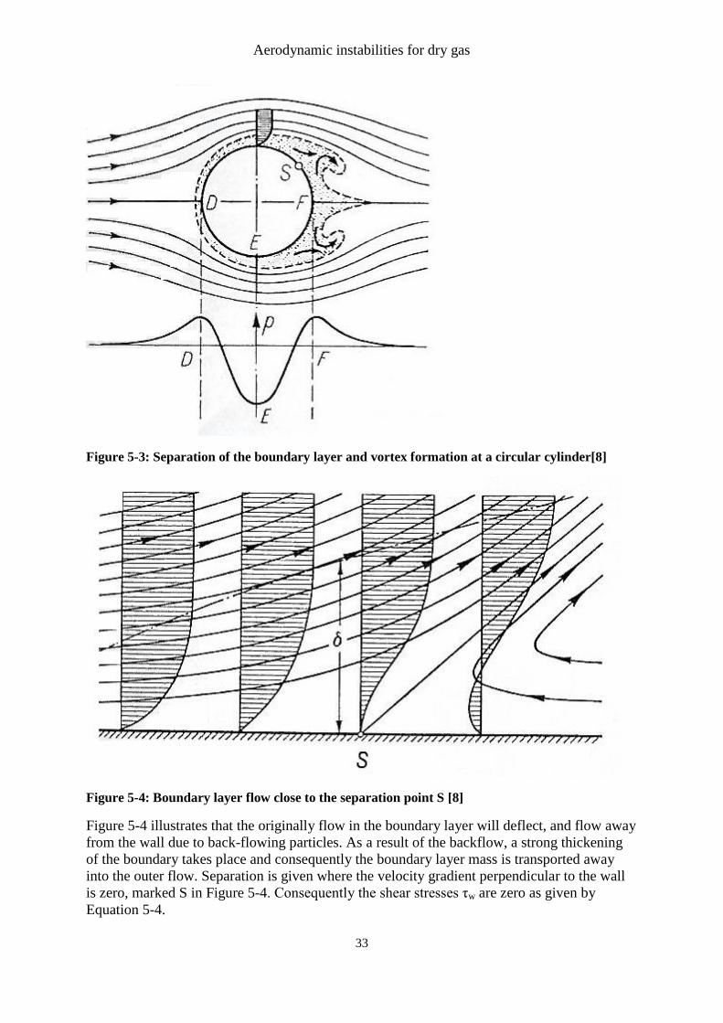
Aerodynamic instabilities for dry gas
33
Figure 5-3: Separation of the boundary layer and vortex formation at a circular cylinder[8]
Figure 5-4: Boundary layer flow close to the separation point S [8]
Figure 5-4 illustrates that the originally flow in the boundary layer will deflect, and flow away
from the wall due to back-flowing particles. As a result of the backflow, a strong thickening
of the boundary takes place and consequently the boundary layer mass is transported away
into the outer flow. Separation is given where the velocity gradient perpendicular to the wall
is zero, marked S in Figure 5-4. Consequently the shear stresses τw are zero as given by
Equation 5-4.
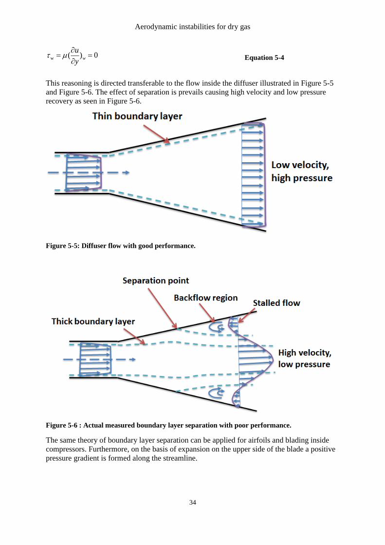
Aerodynamic instabilities for dry gas
34
w ( ) 0w
u
y
Equation 5-4
This reasoning is directed transferable to the flow inside the diffuser illustrated in Figure 5-5
and Figure 5-6. The effect of separation is prevails causing high velocity and low pressure
recovery as seen in Figure 5-6.
Figure 5-5: Diffuser flow with good performance.
Figure 5-6 : Actual measured boundary layer separation with poor performance.
The same theory of boundary layer separation can be applied for airfoils and blading inside
compressors. Furthermore, on the basis of expansion on the upper side of the blade a positive
pressure gradient is formed along the streamline.
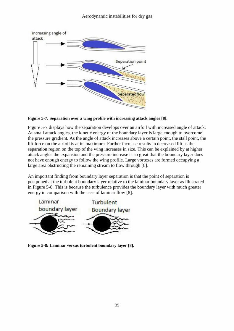
Aerodynamic instabilities for dry gas
35
Figure 5-7: Separation over a wing profile with increasing attack angles [8].
Figure 5-7 displays how the separation develops over an airfoil with increased angle of attack.
At small attack angles, the kinetic energy of the boundary layer is large enough to overcome
the pressure gradient. As the angle of attack increases above a certain point, the stall point, the
lift force on the airfoil is at its maximum. Further increase results in decreased lift as the
separation region on the top of the wing increases in size. This can be explained by at higher
attack angles the expansion and the pressure increase is so great that the boundary layer does
not have enough energy to follow the wing profile. Large vortexes are formed occupying a
large area obstructing the remaining stream to flow through [8].
An important finding from boundary layer separation is that the point of separation is
postponed at the turbulent boundary layer relative to the laminar boundary layer as illustrated
in Figure 5-8. This is because the turbulence provides the boundary layer with much greater
energy in comparison with the case of laminar flow [8].
Figure 5-8: Laminar versus turbulent boundary layer [8].
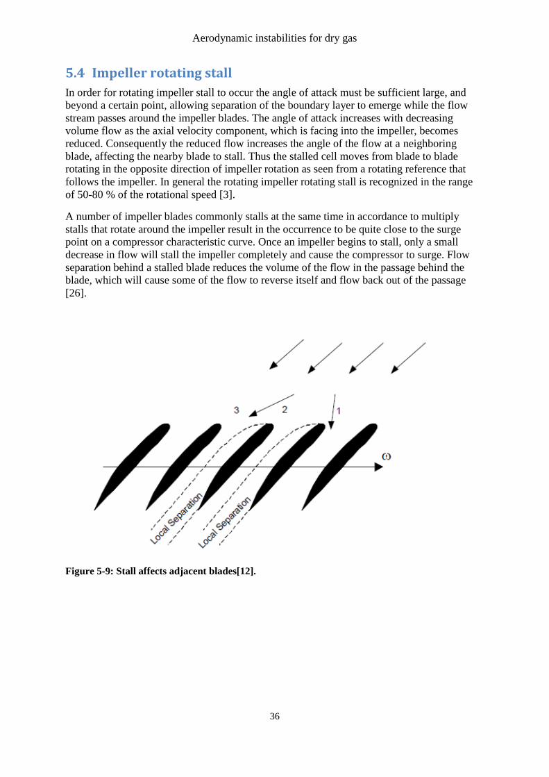
Aerodynamic instabilities for dry gas
36
5.4 Impeller rotating stall
In order for rotating impeller stall to occur the angle of attack must be sufficient large, and
beyond a certain point, allowing separation of the boundary layer to emerge while the flow
stream passes around the impeller blades. The angle of attack increases with decreasing
volume flow as the axial velocity component, which is facing into the impeller, becomes
reduced. Consequently the reduced flow increases the angle of the flow at a neighboring
blade, affecting the nearby blade to stall. Thus the stalled cell moves from blade to blade
rotating in the opposite direction of impeller rotation as seen from a rotating reference that
follows the impeller. In general the rotating impeller rotating stall is recognized in the range
of 50-80 % of the rotational speed [3].
A number of impeller blades commonly stalls at the same time in accordance to multiply
stalls that rotate around the impeller result in the occurrence to be quite close to the surge
point on a compressor characteristic curve. Once an impeller begins to stall, only a small
decrease in flow will stall the impeller completely and cause the compressor to surge. Flow
separation behind a stalled blade reduces the volume of the flow in the passage behind the
blade, which will cause some of the flow to reverse itself and flow back out of the passage
[26].
Figure 5-9: Stall affects adjacent blades[12].
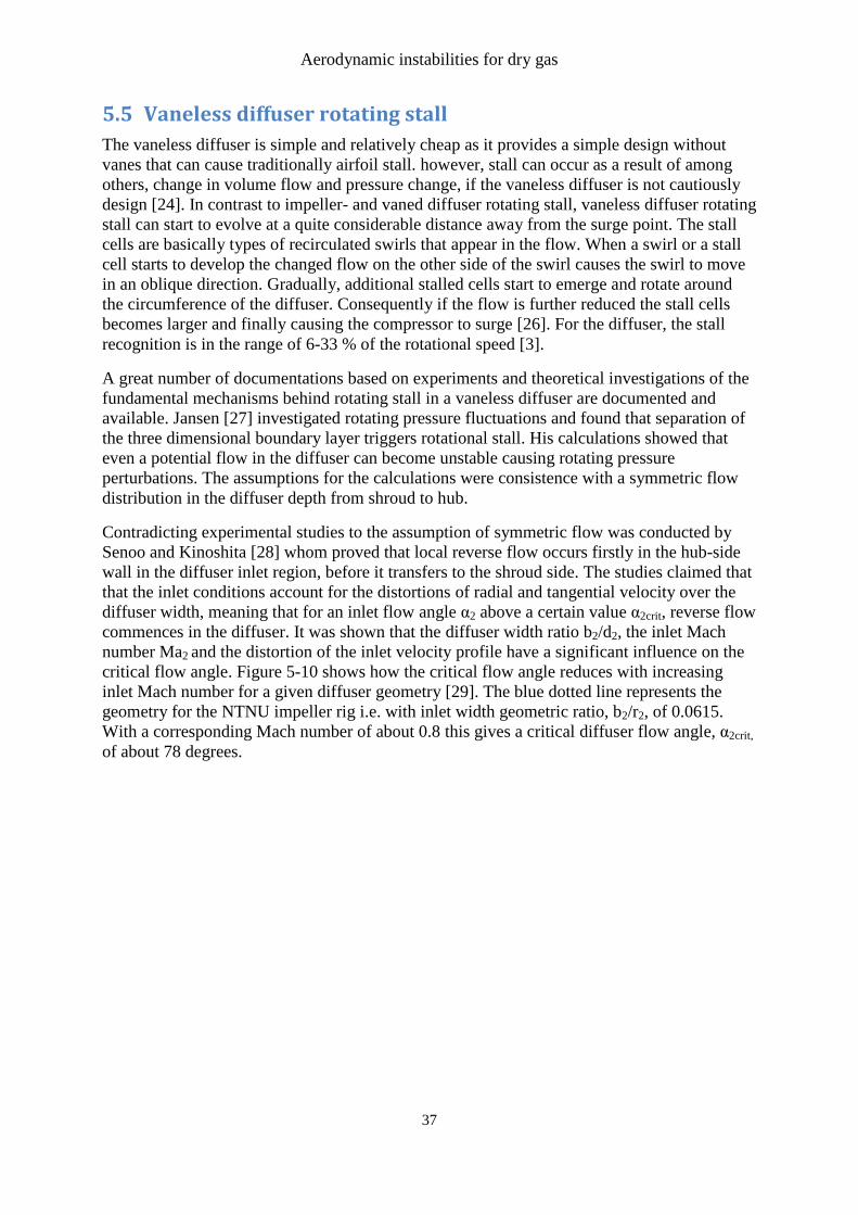
Aerodynamic instabilities for dry gas
37
5.5 Vaneless diffuser rotating stall
The vaneless diffuser is simple and relatively cheap as it provides a simple design without
vanes that can cause traditionally airfoil stall. however, stall can occur as a result of among
others, change in volume flow and pressure change, if the vaneless diffuser is not cautiously
design [24]. In contrast to impeller- and vaned diffuser rotating stall, vaneless diffuser rotating
stall can start to evolve at a quite considerable distance away from the surge point. The stall
cells are basically types of recirculated swirls that appear in the flow. When a swirl or a stall
cell starts to develop the changed flow on the other side of the swirl causes the swirl to move
in an oblique direction. Gradually, additional stalled cells start to emerge and rotate around
the circumference of the diffuser. Consequently if the flow is further reduced the stall cells
becomes larger and finally causing the compressor to surge [26]. For the diffuser, the stall
recognition is in the range of 6-33 % of the rotational speed [3].
A great number of documentations based on experiments and theoretical investigations of the
fundamental mechanisms behind rotating stall in a vaneless diffuser are documented and
available. Jansen [27] investigated rotating pressure fluctuations and found that separation of
the three dimensional boundary layer triggers rotational stall. His calculations showed that
even a potential flow in the diffuser can become unstable causing rotating pressure
perturbations. The assumptions for the calculations were consistence with a symmetric flow
distribution in the diffuser depth from shroud to hub.
Contradicting experimental studies to the assumption of symmetric flow was conducted by
Senoo and Kinoshita [28] whom proved that local reverse flow occurs firstly in the hub-side
wall in the diffuser inlet region, before it transfers to the shroud side. The studies claimed that
that the inlet conditions account for the distortions of radial and tangential velocity over the
diffuser width, meaning that for an inlet flow angle α2 above a certain value α2crit, reverse flow
commences in the diffuser. It was shown that the diffuser width ratio b2/d2, the inlet Mach
number Ma2 and the distortion of the inlet velocity profile have a significant influence on the
critical flow angle. Figure 5-10 shows how the critical flow angle reduces with increasing
inlet Mach number for a given diffuser geometry [29]. The blue dotted line represents the
geometry for the NTNU impeller rig i.e. with inlet width geometric ratio, b2/r2, of 0.0615.
With a corresponding Mach number of about 0.8 this gives a critical diffuser flow angle, α2crit,
of about 78 degrees.
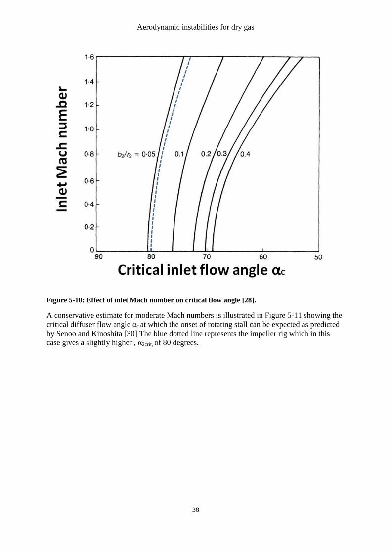
Aerodynamic instabilities for dry gas
38
Figure 5-10: Effect of inlet Mach number on critical flow angle [28].
A conservative estimate for moderate Mach numbers is illustrated in Figure 5-11 showing the
critical diffuser flow angle αc at which the onset of rotating stall can be expected as predicted
by Senoo and Kinoshita [30] The blue dotted line represents the impeller rig which in this
case gives a slightly higher , α2crit, of 80 degrees.
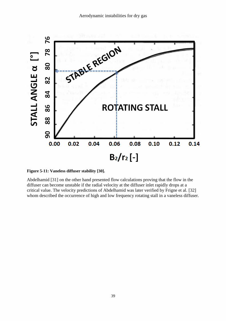
Aerodynamic instabilities for dry gas
39
Figure 5-11: Vaneless diffuser stability [30].
Abdelhamid [31] on the other hand presented flow calculations proving that the flow in the
diffuser can become unstable if the radial velocity at the diffuser inlet rapidly drops at a
critical value. The velocity predictions of Abdelhamid was later verified by Frigne et al. [32]
whom described the occurrence of high and low frequency rotating stall in a vaneless diffuser.
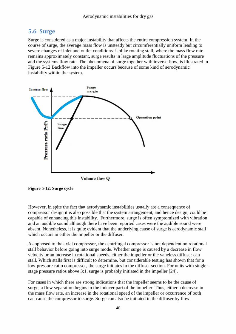
Aerodynamic instabilities for dry gas
40
5.6 Surge
Surge is considered as a major instability that affects the entire compression system. In the
course of surge, the average mass flow is unsteady but circumferentially uniform leading to
severe changes of inlet and outlet conditions. Unlike rotating stall, where the mass flow rate
remains approximately constant, surge results in large amplitude fluctuations of the pressure
and the systems flow rate. The phenomena of surge together with inverse flow, is illustrated in
Figure 5-12.Backflow into the impeller occurs because of some kind of aerodynamic
instability within the system.
Figure 5-12: Surge cycle
However, in spite the fact that aerodynamic instabilities usually are a consequence of
compressor design it is also possible that the system arrangement, and hence design, could be
capable of enhancing this instability. Furthermore, surge is often symptomized with vibration
and an audible sound although there have been reported cases were the audible sound were
absent. Nonetheless, it is quite evident that the underlying cause of surge is aerodynamic stall
which occurs in either the impeller or the diffuser.
As opposed to the axial compressor, the centrifugal compressor is not dependent on rotational
stall behavior before going into surge mode. Whether surge is caused by a decrease in flow
velocity or an increase in rotational speeds, either the impeller or the vaneless diffuser can
stall. Which stalls first is difficult to determine, but considerable testing has shown that for a
low-pressure-ratio compressor, the surge initiates in the diffuser section. For units with single-
stage pressure ratios above 3:1, surge is probably initiated in the impeller [24].
For cases in which there are strong indications that the impeller seems to be the cause of
surge, a flow separation begins in the inducer part of the impeller. Thus, either a decrease in
the mass flow rate, an increase in the rotational speed of the impeller or occurrence of both
can cause the compressor to surge. Surge can also be initiated in the diffuser by flow
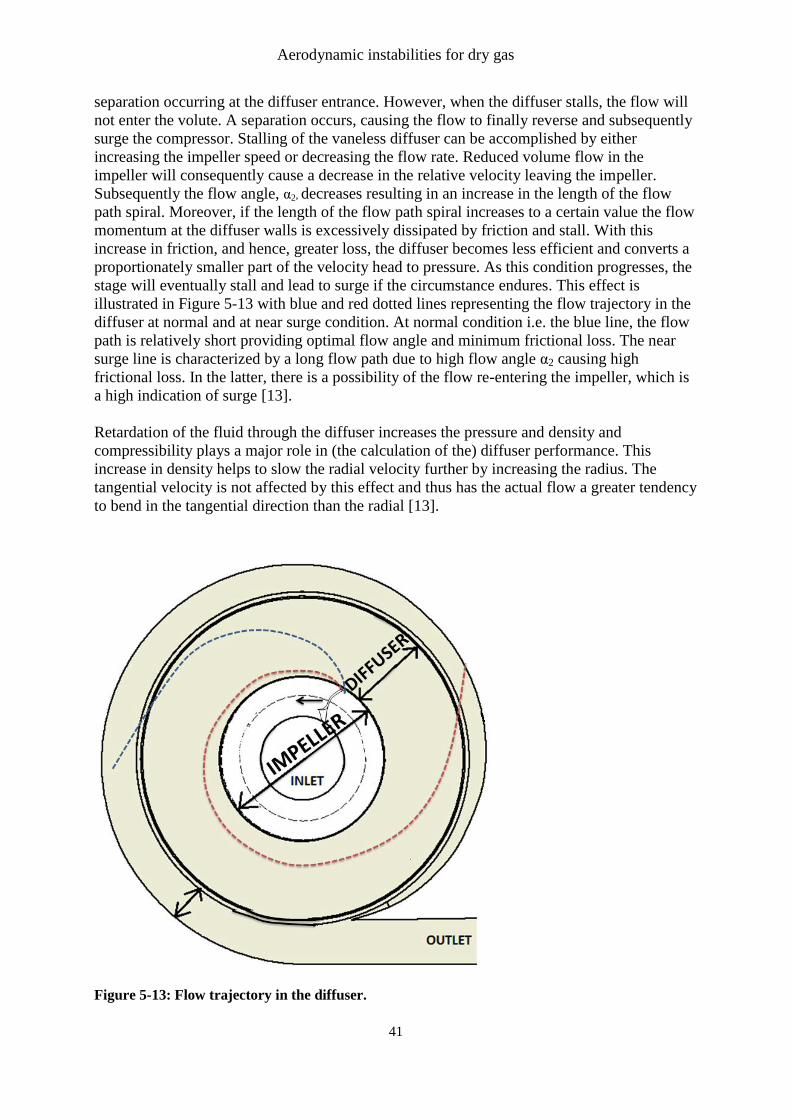
Aerodynamic instabilities for dry gas
41
separation occurring at the diffuser entrance. However, when the diffuser stalls, the flow will
not enter the volute. A separation occurs, causing the flow to finally reverse and subsequently
surge the compressor. Stalling of the vaneless diffuser can be accomplished by either
increasing the impeller speed or decreasing the flow rate. Reduced volume flow in the
impeller will consequently cause a decrease in the relative velocity leaving the impeller.
Subsequently the flow angle, α2, decreases resulting in an increase in the length of the flow
path spiral. Moreover, if the length of the flow path spiral increases to a certain value the flow
momentum at the diffuser walls is excessively dissipated by friction and stall. With this
increase in friction, and hence, greater loss, the diffuser becomes less efficient and converts a
proportionately smaller part of the velocity head to pressure. As this condition progresses, the
stage will eventually stall and lead to surge if the circumstance endures. This effect is
illustrated in Figure 5-13 with blue and red dotted lines representing the flow trajectory in the
diffuser at normal and at near surge condition. At normal condition i.e. the blue line, the flow
path is relatively short providing optimal flow angle and minimum frictional loss. The near
surge line is characterized by a long flow path due to high flow angle α2 causing high
frictional loss. In the latter, there is a possibility of the flow re-entering the impeller, which is
a high indication of surge [13].
Retardation of the fluid through the diffuser increases the pressure and density and
compressibility plays a major role in (the calculation of the) diffuser performance. This
increase in density helps to slow the radial velocity further by increasing the radius. The
tangential velocity is not affected by this effect and thus has the actual flow a greater tendency
to bend in the tangential direction than the radial [13].
Figure 5-13: Flow trajectory in the diffuser.
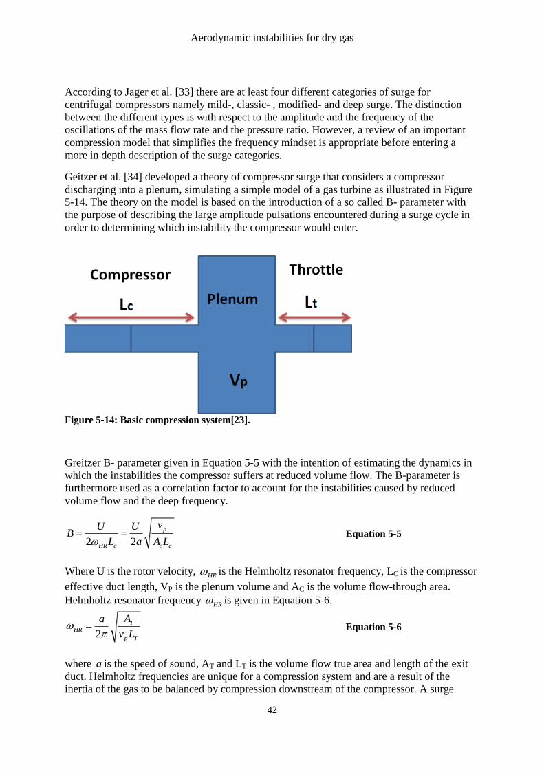
Aerodynamic instabilities for dry gas
42
According to Jager et al. [33] there are at least four different categories of surge for
centrifugal compressors namely mild-, classic- , modified- and deep surge. The distinction
between the different types is with respect to the amplitude and the frequency of the
oscillations of the mass flow rate and the pressure ratio. However, a review of an important
compression model that simplifies the frequency mindset is appropriate before entering a
more in depth description of the surge categories.
Geitzer et al. [34] developed a theory of compressor surge that considers a compressor
discharging into a plenum, simulating a simple model of a gas turbine as illustrated in Figure
5-14. The theory on the model is based on the introduction of a so called B- parameter with
the purpose of describing the large amplitude pulsations encountered during a surge cycle in
order to determining which instability the compressor would enter.
Figure 5-14: Basic compression system[23].
Greitzer B- parameter given in Equation 5-5 with the intention of estimating the dynamics in
which the instabilities the compressor suffers at reduced volume flow. The B-parameter is
furthermore used as a correlation factor to account for the instabilities caused by reduced
volume flow and the deep frequency.
2 2
p
HR c c c
vU UB
L a A L
Equation 5-5
Where U is the rotor velocity, HR is the Helmholtz resonator frequency, LC is the compressor
effective duct length, VP is the plenum volume and AC is the volume flow-through area.
Helmholtz resonator frequency HR is given in Equation 5-6.
2
THR
p T
Aa
v L
Equation 5-6
where a is the speed of sound, AT and LT is the volume flow true area and length of the exit
duct. Helmholtz frequencies are unique for a compression system and are a result of the
inertia of the gas to be balanced by compression downstream of the compressor. A surge
Aerodynamic instabilities for dry gas
43
occurrence with the absence of mass flow inversion, small pressure fluctuations together with
a periodicity governed by the Helmholtz resonance frequency is regarded as a mild surge.
The second version of surge is the classic surge which is on the other hand categorized with
higher amplitude and lower frequency than the mild surge. Nonetheless as with the mild
surge, the occurrence of backflow is not present in the classic surge.
In the modified surge the entire annulus fluctuates in the axial direction forcing the flow to
be unsteady and non-axisymmetric allowing a mix of classic surge and rotational stall to take
place.
Deep surge is the last and generally the most severe form of surge which is associated with
low frequent, large amplitude oscillation and the presence of backflow within the flow, i.e.
inverse flow as seen in Figure 5-12.The deep frequency is considerable lower than the
Helmholtz frequency so in order to determine the effect the Greitzer B-parameter is used to
estimate the dynamic in which the instabilities the compressor suffer at reduced volume flow.
The B-parameter is used as a correlation factor to account for the instabilities caused by
reduced volume flow and the deep frequency [35].
5.7 Chapter summary and conclusion
The aerodynamic stability is in brief the compressors response to disturbance that changes the
operation point of the compressor. The performance of centrifugal compressors is highly
influenced by aerodynamic instabilities and it is important to distinguish between the different
reasons to the aerodynamic instabilities, stall and surge. There are two types of stall reported
for dry gas in a centrifugal compressor namely impeller stall and stall in diffuser. For
centrifugal compressors the stall is created by areas of stalled passages identified as stall cells
occupying volume in the compressor. The operation mode of stall is associated with the
separation of the boundary layer in flow through the compressor. In order for rotating impeller
stall to occur, the angle of attack must be sufficient large, and beyond a certain point, allowing
separation of the boundary layer to emerge while the flow stream passes around the impeller
blades. In general the impeller rotating stall is recognized in the range of 50-80 % of the
rotational speed whereas the range is 6-33 % for the diffuser. Surge is considered as a major
instability that affects the entire compression system. In the course of surge, the average mass
flow is unsteady but circumferentially uniform leading to severe changes of inlet and outlet
conditions. Unlike rotating stall, where the mass flow rate remains approximately constant,
surge results in large amplitude fluctuations of the pressure and the systems flow rate.

Aerodynamic instabilities for dry gas
44
The influence of wet gas for compressor stability
45
6 The influence of wet gas for compressor stability
Surge and stall are two extremely difficult phenomena’s to understand in particular with the presence
of liquid in the flow. Theory and experiments based on injection of water into a dry gas system in
order to investigate instabilities exists, nonetheless especially for axial compressors. Most of the
experiments are brought out on inlet or inter-stage fogging and heavy rain ingestion which will be
outlined in Section 6.1 followed by a literature review associated of stability issues of recently
research on centrifugal compressor subjected to wet gas.
6.1 Fogging and heavy rain ingestion for axial compressors
Water injection in the axial compressor was initially intended for increasing the gas turbine outlet
power when the ambient temperature increases. Fogging and overspray has successfully been applied
in gas turbines worldwide due to its potential to maintain the operation stability of the compressor,
however the technology has not been fully understood.
A research on the influence of fogging on an axial compressor was conducted by Härtel and
Pfeiffer [36] ,it includes a broad coverage of the influence of droplet diameter, relative
humidity and gas volume fraction has on the compressor performance. The findings suggested
that influence of polytrophic efficiency on the gains of high fogging is addressed; meaning
also that operation stability of the machine was retained, hence more effective for
compressors of low efficiency. A Moore Greitzer based model for wet gas compression was
developed by Wang et al [37] simulating different steady state inlet conditions for a S1A-02
gas turbine. The simulations revealed that the pressure- ratio increased and the surge line
moved –up left relative to the dry gas surge line in the compressor map in Figure 5-12. In
other words, wet gas compression can, to a certain extent, eliminate stall and surge and hence
extend the range of stable operation. Similar experiments based on heavy rain ingestion in
terms of large droplets in a axial flow compressor was accompanied by Day et al. [38]
showing contradictory results in comparison to the work regarding inter- stage fogging. A
decrease in both the compressor efficiency and the stability was imminent. The explanation
lies in the fact that after the droplets collide with the first row blades and centrifuged towards
the casing where the normal air flow patterns in the vicinity of the rotor tips are disrupted
causing endwall blocking of the flow channel.
Some concluding remarks are appropriate due to the fact to the existence of consistency related to
centrifugal compression. When the compressor operates near stall, the suited particle diameter for
liquid injection has proven to increase the inlet flow rate and pressure ratio and extend the stable
operation. However, injection of water has also proven adverse effects that decrease the inlet flow rate
and pressure ratio runs at design point when the liquid extend a particular size.
The influence of wet gas for compressor stability
46
6.2 Wet gas centrifugal compressor stability
For wet gas compression in centrifugal compressors it is only during recent years that a
satisfactory amount of research has been accomplished. However, despite the numerous
recent works on this topic, the fundamental understanding of wet gas compression processes
remains challenging. Two of the reasons for this are undefined standards for testing and
performance, and lack of understanding of the basic physical phenomena. Some of the
contributions that have dealt with the wet gas injection in centrifugal compressors related to
instabilities will be discussed here.
Abdelwahab [39] performed calculations for wet gas compression by injection of water in an
industrial centrifugal compressor. The findings revealed that wet gas compression can be used
for centrifugal compression if the droplet size diameter is kept below 5µm. This is due to a
fact that small droplet diameters led to a much faster evaporation time compared to the fluid
particle travel time. The higher the injection rate, the higher the total pressure ratio the stage
could develop. This was due to colder compression temperatures allowing the work
transferred from the impeller to the flow and then converted into higher total pressures.
Brenne et al [40] performed an initial testing to verify multiphase boosting capabilities of a
centrifugal compressor. The testing consisted of performing dynamic pressure measurements
injecting liquid into the compressor. The tests showed that the compressor pressure ratio
increased with increasing gas volume fraction due to rising density of the flowing fluid i.e.
relative to the case of dry gas. Moreover data from the pressure transducers gave strong
indications that the pressure fluctuations within the flow were reduced by the presence of
liquid in the gas stream. In the case of high liquid in the flow the findings indicated that a
reduced blade -pass frequency amplitude emerged with subsequent acoustic reduction
triggering instabilities in the rotor. In experiments brought out by Hundseid et al. [4] a wet gas
compressor test with hydrocarbons were performed at high pressure i.e. ranging from 30-70
bar. The findings suggested that dry gas parameters are not directly applicable for wet gas
performance analysis, nonetheless, Wood’s two phase speed of sound correction model were
used in order to compensate for the different tests. The pressure ratio increased relative to dry
conditions when GVF was decreased. Furthermore, when liquid was present the degradation
linked to performance was noticeable.
Grüner et al. [41] performed experimental analysis on a single airfoil immersed in wet gas
flow and revealed an expanding premature boundary layer separation with reducing gas
volume fractions. At the point of separation a local film thickening followed by increased
liquid film fluctuations was observed. A continuity wave was initiated by deposited and
secondary droplets surrounding the airfoil as a U shape of increased liquid concentration. On
the basis of this it was concluded that the operation characteristics of a compressor changes as
a consequence of the premature separation of the boundary layer caused by liquid impact.
Increased blockage caused by wake formation reduces the effective flow area and increases
the losses whereas the continuity wave causes substantial changes to the inlet flow.
In the work conducted by Fabbrizzi et al. [42] a single stage compressor was used to
investigate the effects of wet gas compression based on variation in the gas mass fraction
GMF (1-0.5) the impeller speed, droplet size and the injection pattern of the liquid. The
results clearly demonstrate that wet gas strongly influences compressor performance,
considering adsorbed power, efficiency and compressor characteristics. The results also show
that, although the impeller design did not account for heavily wet streams, the overall
compression characteristics remain good and the machine was able to process the two-phase
mixture without failures, in some cases with improved pumping. In fact, the compression ratio
The influence of wet gas for compressor stability
47
initially increased for small amounts of injected liquid relative to dry gas and decreased when
the GMF was further decreased. Grüner and Bakken [3] demonstrated through experiments
involving aerodynamic instability investigation of an centrifugal compressor exposed to wet
gas that the compressor encountered a delayed instability inception due to the presence of the
liquid. The findings suggested that the liquid altered the frequency spectrum consisting of
low- frequent throughout the entire compressor characteristic. In addition the compressor
characteristic revealed increased pressure ratio rise to surge with decreasing GMF.
A two- stage wet gas compression campaign was conducted by Ransom et al. [43] in 2011
which focused on characterizing the mechanical performance of the compressor. The
compressor was tested with a various mixture of air and water within a range of GVF varying
from 95% to 100 % for different speed lines while the suction pressure was held at 19 and 20
bara. The pressure ratio increased during the injection of water suggesting that it is directly
related to the increasing Mach number at the stage discharge.
Experimental testing with respect to aerodynamic instabilities for wet gas within a centrifugal
compressor was conducted by the author of this master thesis [11] with guidance from Trond
Grüner. The findings revealed a delayed development of instabilities for wet gas relative to
tests on dry gas. The frequency spectrum analysis performed did not conceal any stall
frequencies which is typical for dry gas before entering surge, suggesting that the compressor
did not attend rotating stall prior to surge. The visual observation from the experiments
showed backflow at the impeller inlet and a deviating liquid flow path for the diffuser with
reduced GMF. However, the observed water backflow in the inlet of the impeller occurs
without pressure fluctuations recorded at the outlet, which may indicate an impeller stall with
zones of reversal flow near the inlet. In the latest work of Grüner and Bakken [44] formation
of an extending annulus ring of liquid was identified at the impeller inlet with reducing
volume flow prior to surge. Droplet entrainment from the ring was revealed with a disordered
flow reversal. Visual observations of the flow inside the diffuser showed a tangential liquid
film flow path suggesting that liquid may be forced to deposit on the pressure side of the
impeller blades due to inertia forces. The high energy in the fluid will affect the gas phase so
that the flow path through the diffuser is shortened with less friction.
Consequently the absolute core angle out of the impeller will be less tangential than the liquid
film flow.

The influence of wet gas for compressor stability
48
Flow visualization techniques
49
7 Flow visualization techniques
A comprehensive evaluation of different visualization techniques related to characterizing
stall and surge for turbo machinery was performed by Dahl [45]. The main purpose was to
determine whether the visualizations techniques could be adopted for the detection of stall and
surge in multiphase flow in the NTNU Impeller rig. The survey consisted of optical and non-
optical visualization measurement techniques. The optical methods includes Laser Doppler
Velocimetry (LDV), Particle Image Velocimetry (PIV), Laser two-focused Velocimetry
(L2F), Doppler Global Velocimetry (DGV) and Pressure Sensitive Paint (PSP). Common for
all of them is the ability to not cause any disturbance within the flow field when implementing
in rotating impeller or diffuser channels because the method uses particles that follow the
flow without the influence of buoyancy effects. The concept of LDV was tested by Dahl [45]
for dry gas purposes on the NTNU impeller rig facility where the measurement was
conducted through the diffuser plexiglas. The system was unfortunately not capable of
detecting the velocities due to glare and reflections from the plexiglas. It was obvious that the
problem would enhance in the case of wet gas implementing due to difficulties in detecting
the particles as they would be hidden because of liquid film development on the diffuser
walls. It was concluded that other optical measurements techniques also would have suffer
from the same problems when implementing wet gas [45].
The non-optical visualization techniques on the other hand, includes Hot-Wire Anemometry
(HWA), Film Anemometry (FA), Pitot static probes, High frequent dynamic- and Static-
pressure sensors. These methods are characterized by high complexity in the shape of the
actual measuring device regarding size and practicability. In addition, complex methods for
data analysis are needed in order to detect the instabilities that occur.
Some of these, non-optical measurement techniques namely high frequent dynamic and static
pressure sensors has showed good results in multiphase analysis of instabilities in the NTNU
impeller rig [45, 46]. High-response dynamic pressure sensors i.e. piezoelectric sensors (PCB)
flush mounted in the diffuser was implemented by Grüner [47] and used for instability
investigations for wet gas in the impeller rig. When wet gas was injected to the compressor,
the PCB sensors detected amplified low frequencies compared to the case of dry gas,
suggesting that dynamic film and droplet impact on the sensing element together with
interference between the phases leading to pressure fluctuations that will be identified in the
frequency analysis. In addition Grüner and Bakken[46] performed an attempt using a pitot
tube for wet gas surge detection for comparison with the PCB sensor arrangement. The pitot
probe was positioned in the opposite direction upstream from the injection module and the
impeller inlet, i.e. not in direct contact with the liquid. The findings from the pitot probe and
the PCB measurements gave synchronously surge indications.
Based on the findings from Grüner regarding pitot probe it was decided to conduct a more in
depth review of pitot probe based measurement devices as a method for wet gas
measurements of instabilities. A literature review of pitot –tube and pitot based measurement
techniques are given in Section 7.1
Flow visualization techniques
50
7.1 Pitot probe investigation
This section are intended for a literature review of the use of pitot tube for compressor dry
and wet gas measurements.
7.1.1 Pitot tube fundamentals and measurement principles
A pitot static tube is essentially a simple device that measures the flow stream velocity. Pitot
tubes are reliable, inexpensive and suited for a variety of environmental conditions, including
extremely high temperatures and a wide range of pressures. A calibrated, clean and properly
inserted pitot tube can provide ±1% of full scale flow accuracy over a low range of 3:1; and,
with some loss of accuracy, it can even measure over a range of 4:1, however a decrease in
the accuracy (up to 5%) is found if not carefully installed. Pitot tubes are generally used for
flow measurements of secondary importance where cost is a major concern, due to additional
limitations including errors from velocity profile changes or from plugging of the pressure
ports [48].
There are generally two types of pitot probe concepts i.e. the pitot static -probe and the simple
pitot probe. For the pitot static probes both the static- and the total impact- pressure are
measured by a small diameter open L-shaped tube facing in opposite and parallel direction of
the stream, illustrated in Figure 7-1. As seen from the figure it is generally two channels in the
tube, i.e. one port for static pressure opening oriented parallel to the flow and one port for the
total impact pressure oriented directed perpendicular to the flow. The static pressure, Pstatic is
the operating pressure upstream to the pitot tube and the total impact pressure Ptot , is the sum
of the static pressure and the total kinetic pressure for one phase measurements are given by
Equation 7-1 [49].
2
2
1
2tot staticP P PV
Equation 7-1
the fluid velocity, V2 are given from the Bernoulli Equation 7-2: 2 2
1 1 2 21 2
2 2
V P V PgZ gZ
Equation 7-2
given the fact that the fluid velocity V1 is at rest at port 1 i.e. equal to 0 and Z is negligible for
gases, V2 becomes:
2 *V C Equation 7-3
From equation 8-2 and 8-3 the pressure difference can be expressed as given by Equation 7-4
below
tot staticP P P Equation 7-4
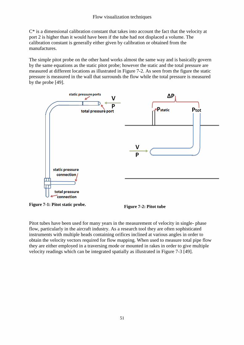
Flow visualization techniques
51
C* is a dimensional calibration constant that takes into account the fact that the velocity at
port 2 is higher than it would have been if the tube had not displaced a volume. The
calibration constant is generally either given by calibration or obtained from the
manufactures.
The simple pitot probe on the other hand works almost the same way and is basically govern
by the same equations as the static pitot probe; however the static and the total pressure are
measured at different locations as illustrated in Figure 7-2. As seen from the figure the static
pressure is measured in the wall that surrounds the flow while the total pressure is measured
by the probe [49].
Figure 7-1: Pitot static probe.
Figure 7-2: Pitot tube
Pitot tubes have been used for many years in the measurement of velocity in single- phase
flow, particularly in the aircraft industry. As a research tool they are often sophisticated
instruments with multiple heads containing orifices inclined at various angles in order to
obtain the velocity vectors required for flow mapping. When used to measure total pipe flow
they are either employed in a traversing mode or mounted in rakes in order to give multiple
velocity readings which can be integrated spatially as illustrated in Figure 7-3 [49].
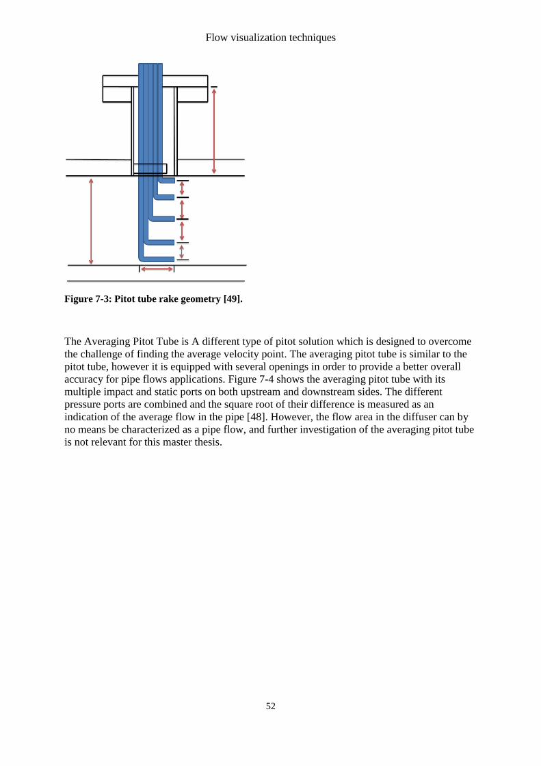
Flow visualization techniques
52
Figure 7-3: Pitot tube rake geometry [49].
The Averaging Pitot Tube is A different type of pitot solution which is designed to overcome
the challenge of finding the average velocity point. The averaging pitot tube is similar to the
pitot tube, however it is equipped with several openings in order to provide a better overall
accuracy for pipe flows applications. Figure 7-4 shows the averaging pitot tube with its
multiple impact and static ports on both upstream and downstream sides. The different
pressure ports are combined and the square root of their difference is measured as an
indication of the average flow in the pipe [48]. However, the flow area in the diffuser can by
no means be characterized as a pipe flow, and further investigation of the averaging pitot tube
is not relevant for this master thesis.
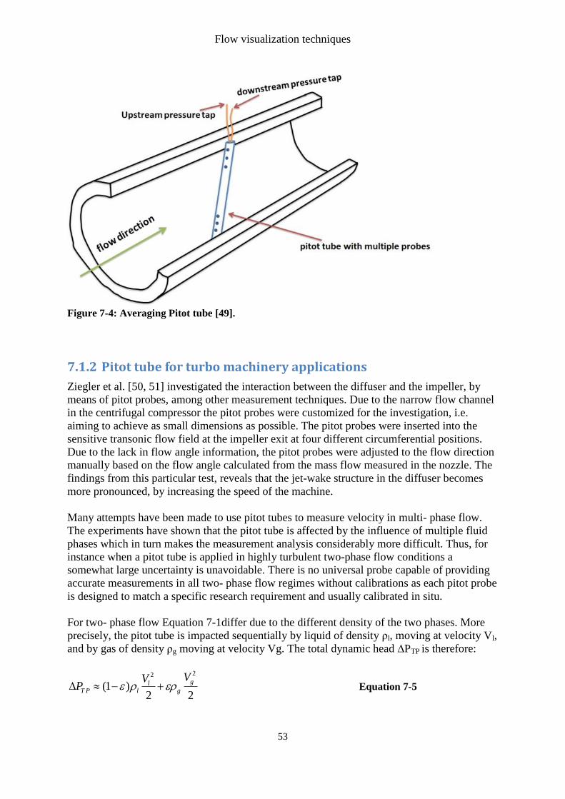
Flow visualization techniques
53
Figure 7-4: Averaging Pitot tube [49].
7.1.2 Pitot tube for turbo machinery applications
Ziegler et al. [50, 51] investigated the interaction between the diffuser and the impeller, by
means of pitot probes, among other measurement techniques. Due to the narrow flow channel
in the centrifugal compressor the pitot probes were customized for the investigation, i.e.
aiming to achieve as small dimensions as possible. The pitot probes were inserted into the
sensitive transonic flow field at the impeller exit at four different circumferential positions.
Due to the lack in flow angle information, the pitot probes were adjusted to the flow direction
manually based on the flow angle calculated from the mass flow measured in the nozzle. The
findings from this particular test, reveals that the jet-wake structure in the diffuser becomes
more pronounced, by increasing the speed of the machine.
Many attempts have been made to use pitot tubes to measure velocity in multi- phase flow.
The experiments have shown that the pitot tube is affected by the influence of multiple fluid
phases which in turn makes the measurement analysis considerably more difficult. Thus, for
instance when a pitot tube is applied in highly turbulent two-phase flow conditions a
somewhat large uncertainty is unavoidable. There is no universal probe capable of providing
accurate measurements in all two- phase flow regimes without calibrations as each pitot probe
is designed to match a specific research requirement and usually calibrated in situ.
For two- phase flow Equation 7-1differ due to the different density of the two phases. More
precisely, the pitot tube is impacted sequentially by liquid of density ρl, moving at velocity Vl,
and by gas of density ρg moving at velocity Vg. The total dynamic head ∆PTP is therefore:
22
2(1 )
2
glT P l g
VVP
Equation 7-5
Flow visualization techniques
54
where is the void fraction. For homogenous flow Vl= Vg=V. Hence 2
2(1 )
2
g mT PM l g
V VP
Equation 7-6
where ρm is the mixture density, provides the following Equation 7-7 for two-phase
homogenous flow:
2* TPM
m
PV C
Equation 7-7
The pitot tube can therefore be used to measure velocity given the mixture density ρm is
known. This simplification is widely used in order to determine the mass flow rate of e.g.
steam and water mixtures in pipes. However, for some flow regimes, the homogenous model
is not suitable. A study by Gill et al [52] concludes that a more generalized expression than
the homogeneous Equation 7-5 must be applied for applications with e.g. droplets in the gas
stream.
2 21(1 )
2tp l l g gP V V
Equation 7-8
In Equation 7-8 σ is 0.5 if the droplets follow the streamlines and if they impact the pitot tube.
However, in practice σ has an intermediate value in which may be dependent on relatively
phase velocities[49].
Despite the theoretical and practical interest in how the multiphase flow will affect the
measurements from the pitot tube, the existing literature on the subject is virtually non-
existent. However, some theory regarding interpreting of pitot pressure measurements in
multiphase flow has been performed on the aerodynamics of wet steam in large steam
turbines. Crane and Moore [45] presented calculations for the flow of wet stream around
purged and unpurged pitot tubes, by means of determining the vapor velocity field around the
tubes using incompressible, potential flow theory assuming that the same velocities field
applies for droplets as well. From momentum loss equations and droplet calculations the
contribution of the droplets to the total pressure rise could be found. Notwithstanding the
important calculations, they did not take into account the likely effect regarding mass transfer
between the liquid droplets and the vapor phase. White et al. [53] on the other hand based the
experimental testing of pitot tube for wet gas flow on the supposition that the flow structure in
a partly disperged shock wave is not very unlike the flow structure between a frozen shock
wave and the pitot head. Frozen meaning that the pitot tube records the pressure as if the
vapor phase alone was brought to rest from the same velocity, assuming that all interface
transfer process remains essentially stationary due to large droplets. The findings showed
good correspondence between total pressure measured downstream of a wet gas steam
cascade operating with condensation shocks, and that predicted by a two-dimensional scheme
for this particular case.
As long as the multiphase flow is thoroughly mixed, the use of pitot tube as measurement
device could be used in conjunction with other devices to measure total mass flow. However,
visualization and measurement of multiphase flow requires a probe that is robust against
liquid droplets, possess high frequency response and cause low impact on the actual flow.
Flow visualization techniques
55
Falcone [49] points out several factors that militate against using pitot tubes in subsea
applications. The book points out factors that include:
The need for a rake and suitable integration procedures
Pipe penetrations and possible probe damage
Intrusiveness: pitot tubes would prevent cleaning
Sensitivity to erosion, corrosion and blockage
The need for multiple connecting lines between the probes and the sensing
instruments.
7.1.3 Pitot probes for wet gas measurements in the NTNU impeller rig.
This sub section discusses the pitot as a measuring device at the NTNU impeller rig. Small
Pitot tube placed inside the diffuser can provide good measurements of the dry gas flow
without affecting the flow to a large extent. A pitot tube will also bypass the problem of liquid
film on the inside of diffusor walls. Equally important is the measurement of the diffuser inlet
angle i.e. an extremely important key parameter for determination of the occurrence of
instabilities in a vaneless diffuser.
Notwithstanding the bypass of the liquid film; the pitot probes are also sensitive to
contaminants in the flow, as these can clog the small holes in the probe. Regarding wet gas
flow, the water will in worst case either clog or penetrate the holes and potentially fill them.
Airplanes operate often in wet environments and uses Pitot tubes to calculate speed. They
solve this problem by heating the Pitot tube so that water and other contaminants vaporize, or
burn up. Similarly, the same method can be used in the diffuser, allowing the surrounding
flow to be heated, resulting in expanded flow and subsequently increased speed.
Instead, a flush system that periodically blow channels in the pitot tube clean will conceivably
work. Since the droplets in the flow are spread, it will take some time for the droplets to hit
the holes in the Pitot tube. In this time interval with dry pitot tubes, it is possible that the
velocities can be measured.
7.2 Pitot- based measuring devices
This Section discusses two other pitot based measuring techniques. A better understanding of
the unsteady flow phenomena such as secondary flow or rotor- stator interactions is a key to
further improvements in turbo machinery. In addition to complex CFD methods modern
measurements techniques with time resolving capabilities are necessary to determine the
instantaneous flow quantities.
7.2.1 Fast- Response Aerodynamic Probe measurement system
The Fast- Response Aerodynamic Probe measurement system (FRAP) are developed at the
Turbo machinery Lab of the Institute of Energy Technology (ETH) in Zurich. FRAP probes
are a promising alternative to other time resolved measurement techniques, such as hot-wire
anemometry or laser techniques that was mentioned at the beginning of Chapter 0). In
Flow visualization techniques
56
addition to the flow angles, Mach number, and velocity, FRAP can additionally measure both
time-resolved total and static pressures. All these flow quantities are determined from the
pressure levels and fluctuations at different points of the probe tip measured with miniature
piezoresistive pressure sensor chips. The FRAP probes provides a high-performance system
primarily dedicated to turbo machinery applications. The one sensor probe, operating as
pseudo-three sensor probes, have shown a high potential because it combines the simple
application and evaluation methods with detailed information about the time-resolved flow
patterns [54]. The current improvement of selected components make the FRAP system suited
for more complex applications, such as detailed-two- dimensional flow field measurements or
even three- dimensional with four sensor probes. The system has been successfully used for
measurement campaigns in different turbo machines at the ETH and in industrial test
facilities[54]. The FRAP probes are able to measure high frequency rotor- governed
systematic fluctuations (like blade to blade phenomena) alone or in combination with flow-
governed low- frequency fluctuations as rotating stall and mild surge. However, three sensor
probes would be needed to measure stochastic (turbulence-related) or other aperiodic velocity
transients [55].
As a consequence of increasing demand of customized probe measuring devices several
research groups worldwide have developed their own probes custom made to their
applications. Hence the FRAP probes has experienced regular improvements, particularly in
terms of diameter reduction since it was invented. Roduner et al. [55] measured time-
resolved flow quantities in a centrifugal compressor using a cylinder shape 3- sensor probe of
a diameter of 1.8 mm. A further reduction of the probe head to 0.84 mm was achieved by
Schlienenger et al. [56] in order to perform measurements of the cavity flow in labyrinth seals
of an axial compressor. In the recent work of Porecco et al. [57] a newly designed 2- sensor
FRAP probe was used in a virtual 4- sensor mode to yield measurements of non- isotropic
turbulence in a multi-stage axial turbine. Moreover a novel high temperature fast response
aerodynamic probe has been developed, built and tested which is based on the virtual 4-
sensor probe. The probe can be applied in flows with temperatures up to 533 K (806 °C) and
can measure three dimensional and unsteady flows up to the cut-off frequency of 25 kHz,
covering flow angles of ±24° in yaw and ±20° in pitch direction. Furthermore, the probe is
able to measure the steady flow temperature [58].
Roduner et al. [55] investigated the impeller exit and the vaned diffuser of a single- stage
high- subsonic centrifugal compressor by the use of FRAP probes in order to detect rotating
stall and surge at stable and unstable running conditions. The probes were mounted in eleven
different positions I to XI at the front wall of the diffuser as seen from Figure 7-5 and Figure
7-6. The position I is highlighted in Figure 7-7. Further the investigation concluded that even
the one sensor FRAP probe was a valuable tool for investigating time- dependent systematic
flow phenomena occurring in turbo machines. A highly detailed insight into blade passing,
mild surge and rotating stall can be achieved not only qualitatively but quantitatively with
high accuracy and resolution.
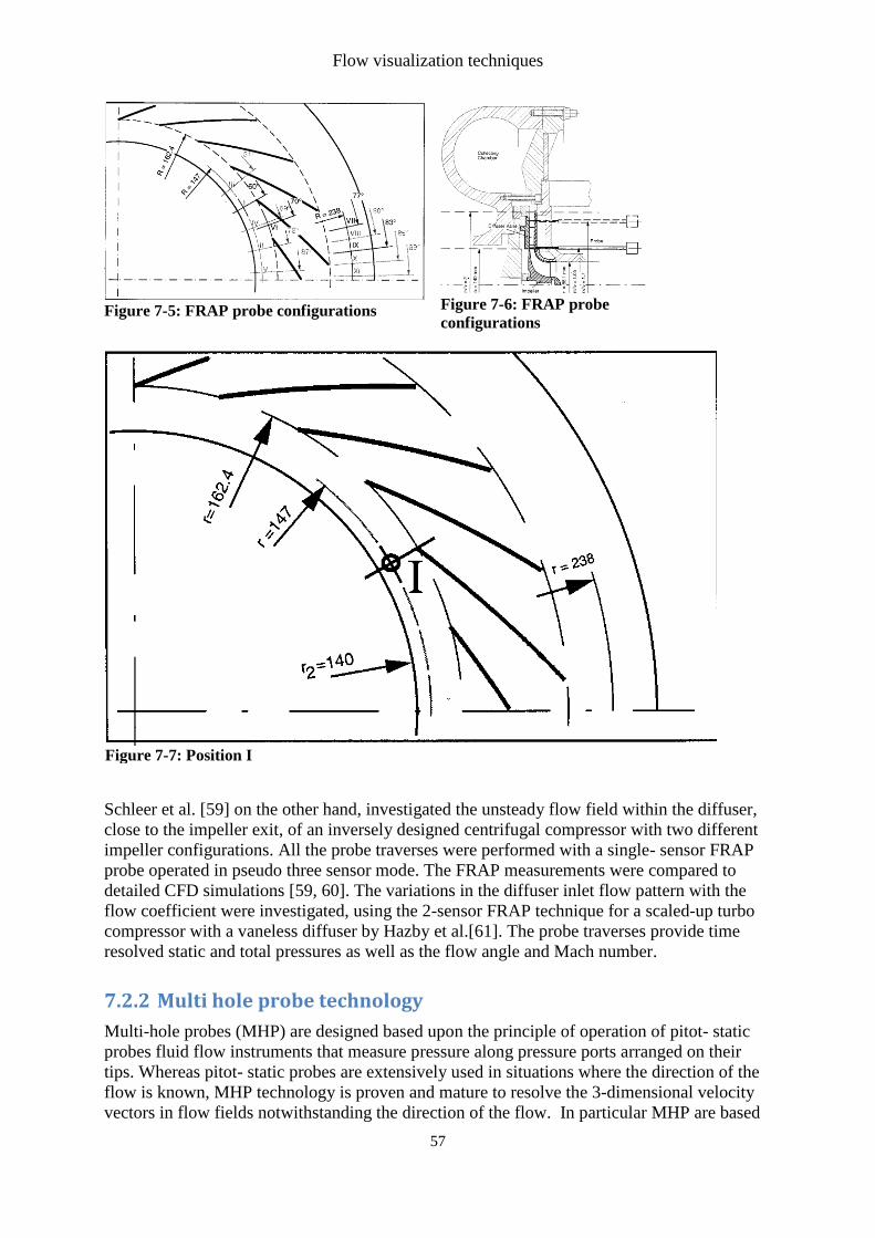
Flow visualization techniques
57
Figure 7-5: FRAP probe configurations
Figure 7-6: FRAP probe
configurations
Figure 7-7: Position I
Schleer et al. [59] on the other hand, investigated the unsteady flow field within the diffuser,
close to the impeller exit, of an inversely designed centrifugal compressor with two different
impeller configurations. All the probe traverses were performed with a single- sensor FRAP
probe operated in pseudo three sensor mode. The FRAP measurements were compared to
detailed CFD simulations [59, 60]. The variations in the diffuser inlet flow pattern with the
flow coefficient were investigated, using the 2-sensor FRAP technique for a scaled-up turbo
compressor with a vaneless diffuser by Hazby et al.[61]. The probe traverses provide time
resolved static and total pressures as well as the flow angle and Mach number.
7.2.2 Multi hole probe technology
Multi-hole probes (MHP) are designed based upon the principle of operation of pitot- static
probes fluid flow instruments that measure pressure along pressure ports arranged on their
tips. Whereas pitot- static probes are extensively used in situations where the direction of the
flow is known, MHP technology is proven and mature to resolve the 3-dimensional velocity
vectors in flow fields notwithstanding the direction of the flow. In particular MHP are based
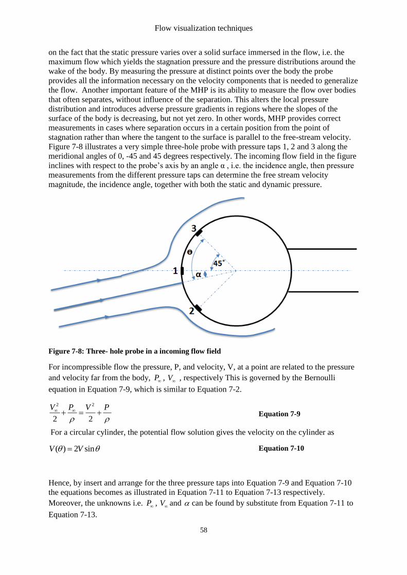
Flow visualization techniques
58
on the fact that the static pressure varies over a solid surface immersed in the flow, i.e. the
maximum flow which yields the stagnation pressure and the pressure distributions around the
wake of the body. By measuring the pressure at distinct points over the body the probe
provides all the information necessary on the velocity components that is needed to generalize
the flow. Another important feature of the MHP is its ability to measure the flow over bodies
that often separates, without influence of the separation. This alters the local pressure
distribution and introduces adverse pressure gradients in regions where the slopes of the
surface of the body is decreasing, but not yet zero. In other words, MHP provides correct
measurements in cases where separation occurs in a certain position from the point of
stagnation rather than where the tangent to the surface is parallel to the free-stream velocity.
Figure 7-8 illustrates a very simple three-hole probe with pressure taps 1, 2 and 3 along the
meridional angles of 0, -45 and 45 degrees respectively. The incoming flow field in the figure
inclines with respect to the probe’s axis by an angle α , i.e. the incidence angle, then pressure
measurements from the different pressure taps can determine the free stream velocity
magnitude, the incidence angle, together with both the static and dynamic pressure.
Figure 7-8: Three- hole probe in a incoming flow field
For incompressible flow the pressure, P, and velocity, V, at a point are related to the pressure
and velocity far from the body, P , V , respectively This is governed by the Bernoulli
equation in Equation 7-9, which is similar to Equation 7-2.
2 2
2 2
V P V P
Equation 7-9
For a circular cylinder, the potential flow solution gives the velocity on the cylinder as
( ) 2 sinV V Equation 7-10
Hence, by insert and arrange for the three pressure taps into Equation 7-9 and Equation 7-10
the equations becomes as illustrated in Equation 7-11 to Equation 7-13 respectively.
Moreover, the unknowns i.e. P , V and can be found by substitute from Equation 7-11 to
Equation 7-13.
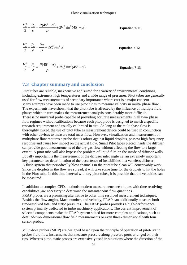
Flow visualization techniques
59
22
2(45 )2 45
2sin ( )
V P PV
Equation 7-11
22 2si
2n2
V P PV
Equation 7-12
22
2(45 )2 45
2sin ( )
V P PV
Equation 7-13
7.3 Chapter summary and conclusion
Pitot tubes are reliable, inexpensive and suited for a variety of environmental conditions,
including extremely high temperatures and a wide range of pressures. Pitot tubes are generally
used for flow measurements of secondary importance where cost is a major concern
Many attempts have been made to use pitot tubes to measure velocity in multi- phase flow.
The experiments have shown that the pitot tube is affected by the influence of multiple fluid
phases which in turn makes the measurement analysis considerably more difficult.
There is no universal probe capable of providing accurate measurements in all two- phase
flow regimes without calibrations because each pitot probe is designed to match a specific
research requirement and usually calibrated in situ. As long as the multiphase flow is
thoroughly mixed, the use of pitot tube as measurement device could be used in conjunction
with other devices to measure total mass flow. However, visualization and measurement of
multiphase flow requires a probe that is robust against liquid droplets, possess high frequency
response and cause low impact on the actual flow. Small Pitot tubes placed inside the diffuser
can provide good measurements of the dry gas flow without affecting the flow to a large
extent. A pitot tube will also bypass the problem of liquid film on the inside of diffusor walls.
Equally important is the measurement of the diffuser inlet angle i.e. an extremely important
key parameter for determination of the occurrence of instabilities in a vaneless diffuser.
A flush system that periodically blow channels in the pitot tube clean will conceivably work.
Since the droplets in the flow are spread, it will take some time for the droplets to hit the holes
in the Pitot tube. In this time interval with dry pitot tubes, it is possible that the velocities can
be measured.
In addition to complex CFD, methods modern measurements techniques with time resolving
capabilities ,are necessary to determine the instantaneous flow quantities.
FRAP probes are a promising alternative to other time resolved measurement techniques.
Besides the flow angles, Mach number, and velocity, FRAP can additionally measure both
time-resolved total and static pressures. The FRAP probes provides a high-performance
system primarily dedicated to turbo machinery applications. The current improvement of
selected components make the FRAP system suited for more complex applications, such as
detailed-two- dimensional flow field measurements or even three- dimensional with four
sensor probes.
Multi-hole probes (MHP) are designed based upon the principle of operation of pitot- static
probes fluid flow instruments that measure pressure along pressure ports arranged on their
tips. Whereas pitot- static probes are extensively used in situations where the direction of the

Flow visualization techniques
60
flow is known, MHP technology is proven and mature to resolve the 3-dimensional velocity
vectors in flow fields notwithstanding the direction of the flow.
Description of experimental setup and procedure
61
8 Description of experimental setup and procedure
This chapter presents the specifications and the changes conducted in the impeller rig
exclusively for this master thesis. The first section is reserved a conclusive summary of the
findings that form the basis for the focus of this master thesis that is given in Section 8.2. A
description of the arrangement of the measuring devices is included in Section 8.3 and 8.4.
8.1 Summary previous work
This Section is intended as a point wise representation of the key findings and observations
made from the pre project of this master thesis [11] regarding instabilities for dry and wet gas
compression. The experimental tests performed in the project thesis confirmed depiction of
recently research concerning instabilities. Other important findings was:
The frequency spectrum concealed a stall propagation that approached the
impeller frequency at reduced flow rate for dry gas, overlapped by the
development of sub-sequent stall frequency propagation.
The phase-lag analysis detected altered tendencies in the phase shift for dry gas,
i.e. deviation in the stall propagation around the circumference of the diffuser.
The compressor characteristic revealed increased pressure ratio rise prior to surge
for wet gas with decreasing gas mass fractions.
Tests showed a tendency of delayed development of instabilities for wet gas
compared to the case of dry gas.
The frequency spectrum for wet gas did not reveal any stall frequencies which is
typical for dry gas before entering surge. However, it gave an indication of the
impact of the reduced GMF had on the surge formation.
Visual observation showed backflow at the impeller inlet for wet gas and a
deviating liquid flow path in the diffuser [11].
8.2 Focus of experiment
Based on the findings described in Section 8.1, together with important findings by Grüner
and Bakken [46], there was an essential necessity to further document the phenomena related
to wet gas surge, especially regarding validation of flow pattern and instability. It was chosen
to conduct experiments on the identification of the impeller outlet angle in order to describe
the diffuser flow pattern. In addition it was chosen to perform experiments on achieving a
more precise identification of the wet gas surge initiation and instability precursors. The main
bullet points were thus to:
Validate the flow pattern at the outlet of the impeller by using pitot measurements.
Identify wet gas surge using wet gas pitot probes.
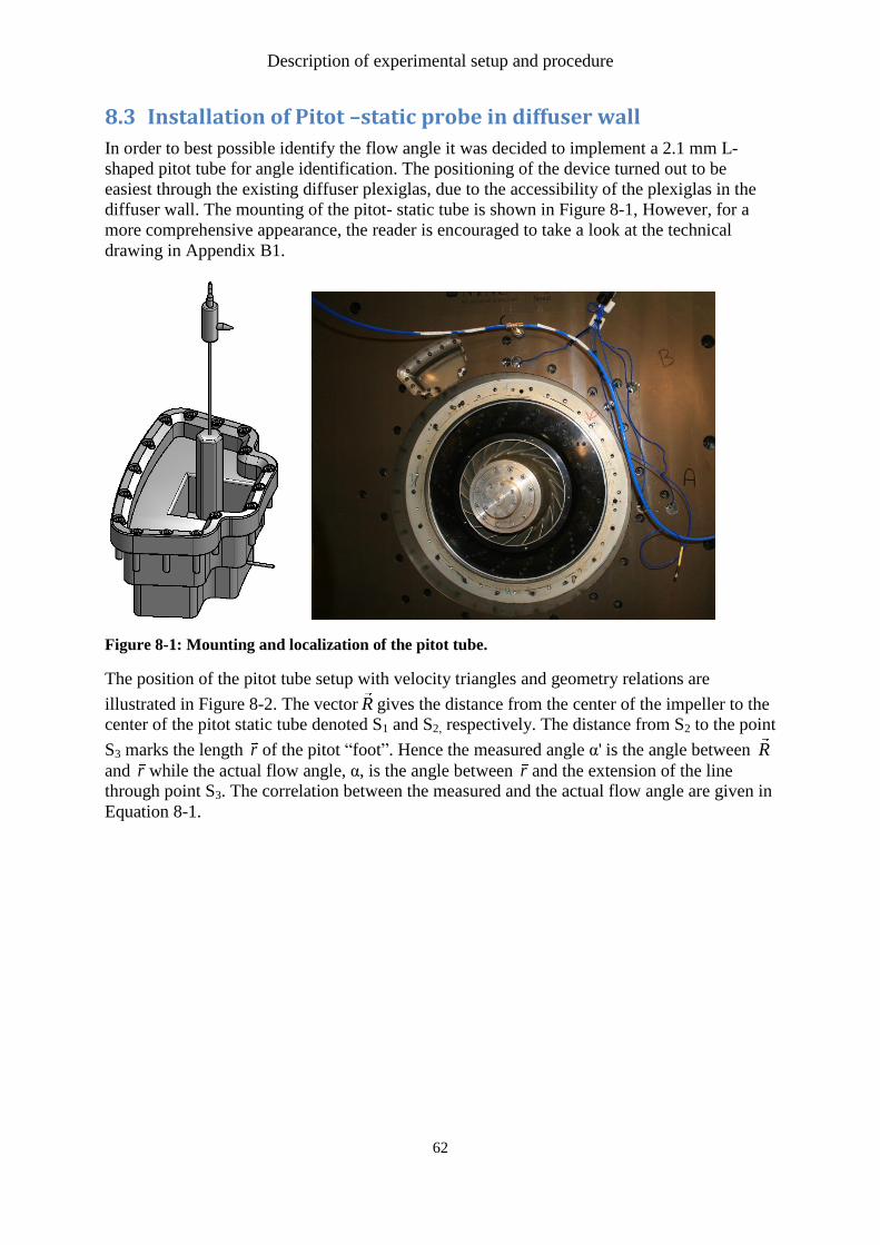
Description of experimental setup and procedure
62
8.3 Installation of Pitot –static probe in diffuser wall
In order to best possible identify the flow angle it was decided to implement a 2.1 mm L-
shaped pitot tube for angle identification. The positioning of the device turned out to be
easiest through the existing diffuser plexiglas, due to the accessibility of the plexiglas in the
diffuser wall. The mounting of the pitot- static tube is shown in Figure 8-1, However, for a
more comprehensive appearance, the reader is encouraged to take a look at the technical
drawing in Appendix B1.
Figure 8-1: Mounting and localization of the pitot tube.
The position of the pitot tube setup with velocity triangles and geometry relations are
illustrated in Figure 8-2. The vector R gives the distance from the center of the impeller to the
center of the pitot static tube denoted S1 and S2, respectively. The distance from S2 to the point
S3 marks the length r of the pitot “foot”. Hence the measured angle α' is the angle between R
and r while the actual flow angle, α, is the angle between r and the extension of the line
through point S3. The correlation between the measured and the actual flow angle are given in
Equation 8-1.
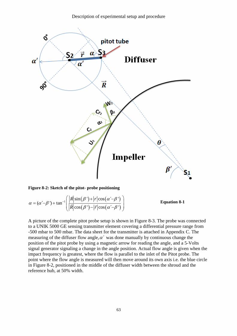
Description of experimental setup and procedure
63
Figure 8-2: Sketch of the pitot- probe positioning
1
sin ' cos ´ '( ´ ') tan
cos ' cos ´ '
R r
R r
Equation 8-1
A picture of the complete pitot probe setup is shown in Figure 8-3. The probe was connected
to a UNIK 5000 GE sensing transmitter element covering a differential pressure range from
-500 mbar to 500 mbar. The data sheet for the transmitter is attached in Appendix C. The
measuring of the diffuser flow angle, ´ was done manually by continuous change the
position of the pitot probe by using a magnetic arrow for reading the angle, and a 5-Volts
signal generator signaling a change in the angle position. Actual flow angle is given when the
impact frequency is greatest, where the flow is parallel to the inlet of the Pitot probe. The
point where the flow angle is measured will then move around its own axis i.e. the blue circle
in Figure 8-2, positioned in the middle of the diffuser width between the shroud and the
reference hub, at 50% width.
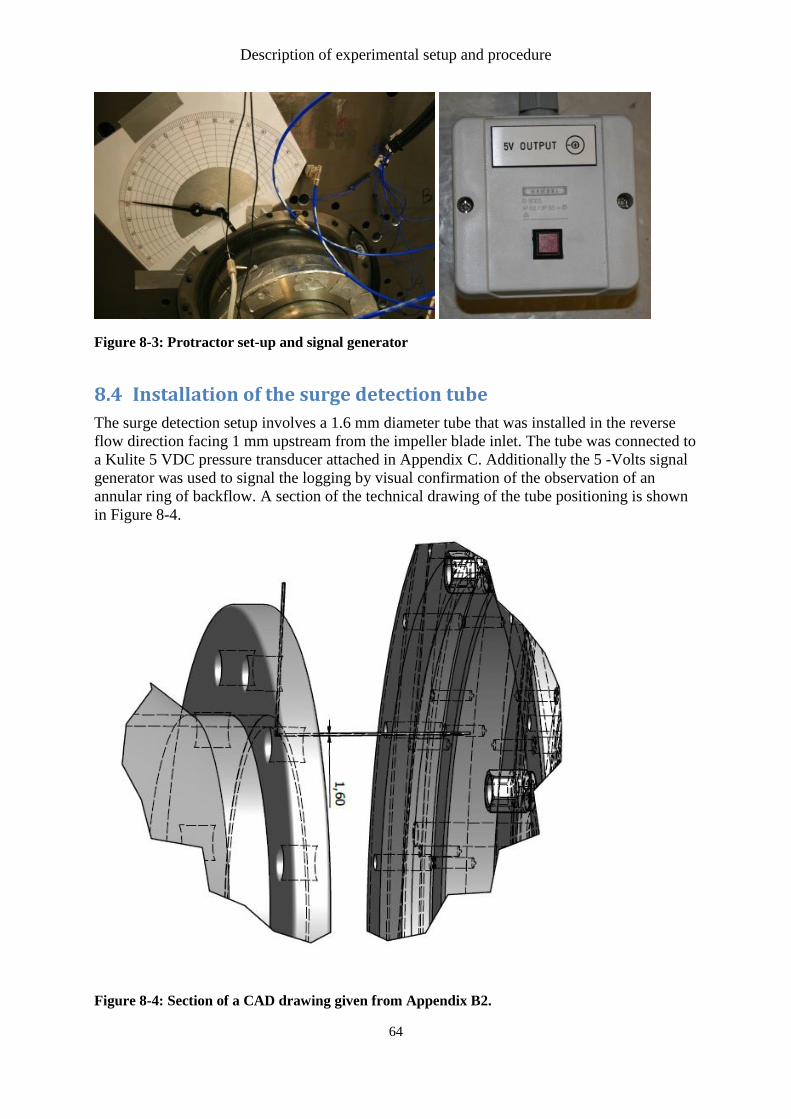
Description of experimental setup and procedure
64
Figure 8-3: Protractor set-up and signal generator
8.4 Installation of the surge detection tube
The surge detection setup involves a 1.6 mm diameter tube that was installed in the reverse
flow direction facing 1 mm upstream from the impeller blade inlet. The tube was connected to
a Kulite 5 VDC pressure transducer attached in Appendix C. Additionally the 5 -Volts signal
generator was used to signal the logging by visual confirmation of the observation of an
annular ring of backflow. A section of the technical drawing of the tube positioning is shown
in Figure 8-4.
Figure 8-4: Section of a CAD drawing given from Appendix B2.
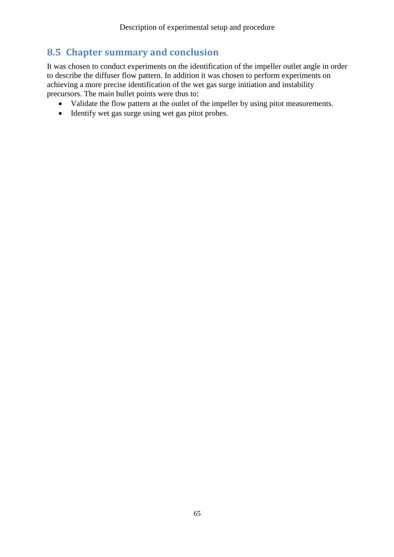
Description of experimental setup and procedure
65
8.5 Chapter summary and conclusion
It was chosen to conduct experiments on the identification of the impeller outlet angle in order
to describe the diffuser flow pattern. In addition it was chosen to perform experiments on
achieving a more precise identification of the wet gas surge initiation and instability
precursors. The main bullet points were thus to:
Validate the flow pattern at the outlet of the impeller by using pitot measurements.
Identify wet gas surge using wet gas pitot probes.

Description of experimental setup and procedure
66
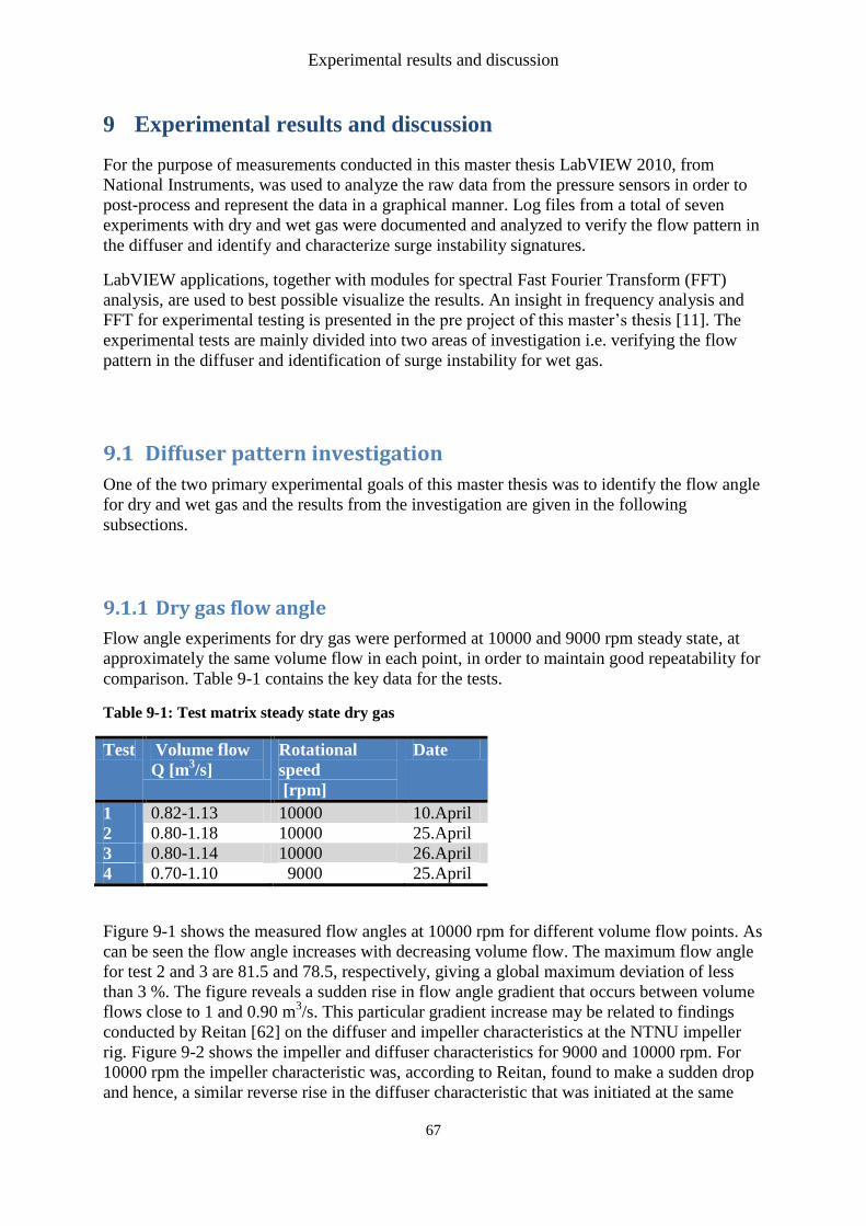
Experimental results and discussion
67
9 Experimental results and discussion
For the purpose of measurements conducted in this master thesis LabVIEW 2010, from
National Instruments, was used to analyze the raw data from the pressure sensors in order to
post-process and represent the data in a graphical manner. Log files from a total of seven
experiments with dry and wet gas were documented and analyzed to verify the flow pattern in
the diffuser and identify and characterize surge instability signatures.
LabVIEW applications, together with modules for spectral Fast Fourier Transform (FFT)
analysis, are used to best possible visualize the results. An insight in frequency analysis and
FFT for experimental testing is presented in the pre project of this master’s thesis [11]. The
experimental tests are mainly divided into two areas of investigation i.e. verifying the flow
pattern in the diffuser and identification of surge instability for wet gas.
9.1 Diffuser pattern investigation
One of the two primary experimental goals of this master thesis was to identify the flow angle
for dry and wet gas and the results from the investigation are given in the following
subsections.
9.1.1 Dry gas flow angle
Flow angle experiments for dry gas were performed at 10000 and 9000 rpm steady state, at
approximately the same volume flow in each point, in order to maintain good repeatability for
comparison. Table 9-1 contains the key data for the tests.
Table 9-1: Test matrix steady state dry gas
Test Volume flow
Q [m3/s]
Rotational
speed
[rpm]
Date
1 0.82-1.13 10000 10.April
2 0.80-1.18 10000 25.April
3 0.80-1.14 10000 26.April
4 0.70-1.10 9000 25.April
Figure 9-1 shows the measured flow angles at 10000 rpm for different volume flow points. As
can be seen the flow angle increases with decreasing volume flow. The maximum flow angle
for test 2 and 3 are 81.5 and 78.5, respectively, giving a global maximum deviation of less
than 3 %. The figure reveals a sudden rise in flow angle gradient that occurs between volume
flows close to 1 and 0.90 m3/s. This particular gradient increase may be related to findings
conducted by Reitan [62] on the diffuser and impeller characteristics at the NTNU impeller
rig. Figure 9-2 shows the impeller and diffuser characteristics for 9000 and 10000 rpm. For
10000 rpm the impeller characteristic was, according to Reitan, found to make a sudden drop
and hence, a similar reverse rise in the diffuser characteristic that was initiated at the same
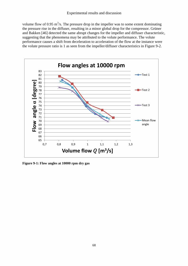
Experimental results and discussion
68
volume flow of 0.95 m3/s. The pressure drop in the impeller was to some extent dominating
the pressure rise in the diffuser, resulting in a minor global drop for the compressor. Grüner
and Bakken [46] detected the same abrupt changes for the impeller and diffuser characteristic,
suggesting that the phenomena may be attributed to the volute performance. The volute
performance causes a shift from deceleration to acceleration of the flow at the instance were
the volute pressure ratio is 1 as seen from the impeller/diffuser characteristics in Figure 9-2.
Figure 9-1: Flow angles at 10000 rpm dry gas
65666768697071727374757677787980818283
0,7 0,8 0,9 1 1,1 1,2 1,3
Flo
w a
ngl
e α
[d
egre
e]
Volume flow 𝑄 [m3/s]
Flow angles at 10000 rpm
Test 1
Test 2
Test 3
Mean flowangle
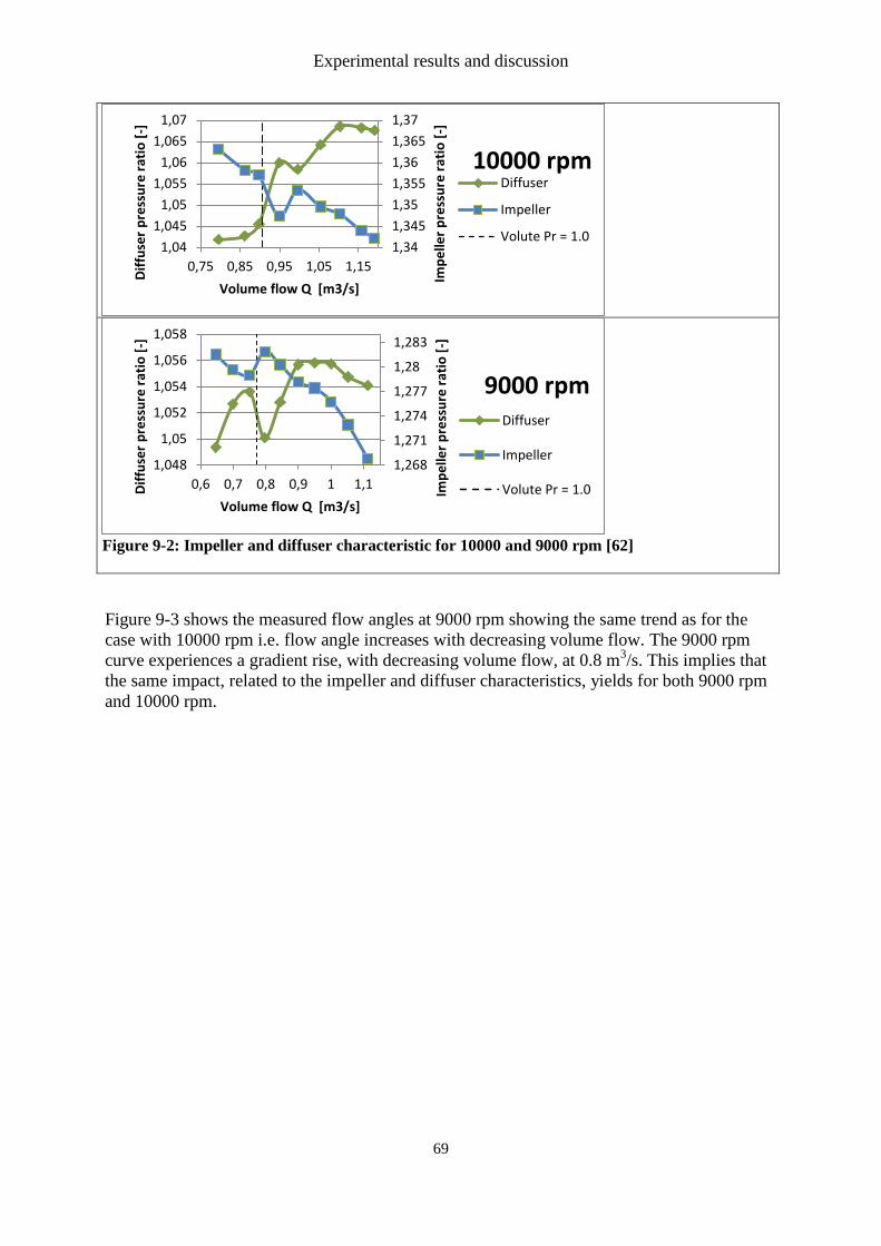
Experimental results and discussion
69
Figure 9-2: Impeller and diffuser characteristic for 10000 and 9000 rpm [62]
Figure 9-3 shows the measured flow angles at 9000 rpm showing the same trend as for the
case with 10000 rpm i.e. flow angle increases with decreasing volume flow. The 9000 rpm
curve experiences a gradient rise, with decreasing volume flow, at 0.8 m3/s. This implies that
the same impact, related to the impeller and diffuser characteristics, yields for both 9000 rpm
and 10000 rpm.
1,34
1,345
1,35
1,355
1,36
1,365
1,37
1,04
1,045
1,05
1,055
1,06
1,065
1,07
0,75 0,85 0,95 1,05 1,15
Imp
elle
r p
ress
ure
rat
io [
-]
Dif
fuse
r p
ress
ure
rat
io [
-]
Volume flow Q [m3/s]
10000 rpm Diffuser
Impeller
Volute Pr = 1.0
1,268
1,271
1,274
1,277
1,28
1,283
1,048
1,05
1,052
1,054
1,056
1,058
0,6 0,7 0,8 0,9 1 1,1
Imp
elle
r p
ress
ure
rat
io [
-]
Dif
fuse
r p
ress
ure
rat
io [
-]
Volume flow Q [m3/s]
9000 rpm Diffuser
Impeller
Volute Pr = 1.0
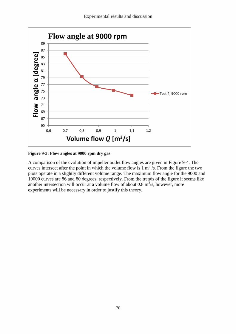
Experimental results and discussion
70
Figure 9-3: Flow angles at 9000 rpm dry gas
A comparison of the evolution of impeller outlet flow angles are given in Figure 9-4. The
curves intersect after the point in which the volume flow is 1 m3 /s. From the figure the two
plots operate in a slightly different volume range. The maximum flow angle for the 9000 and
10000 curves are 86 and 80 degrees, respectively. From the trends of the figure it seems like
another intersection will occur at a volume flow of about 0.8 m3/s, however, more
experiments will be necessary in order to justify this theory.
65
67
69
71
73
75
77
79
81
83
85
87
89
0,6 0,7 0,8 0,9 1 1,1 1,2
Flo
w a
ngl
e α
[d
egr
ee
]
Volume flow 𝑄 [m3/s]
Flow angle at 9000 rpm
Test 4, 9000 rpm
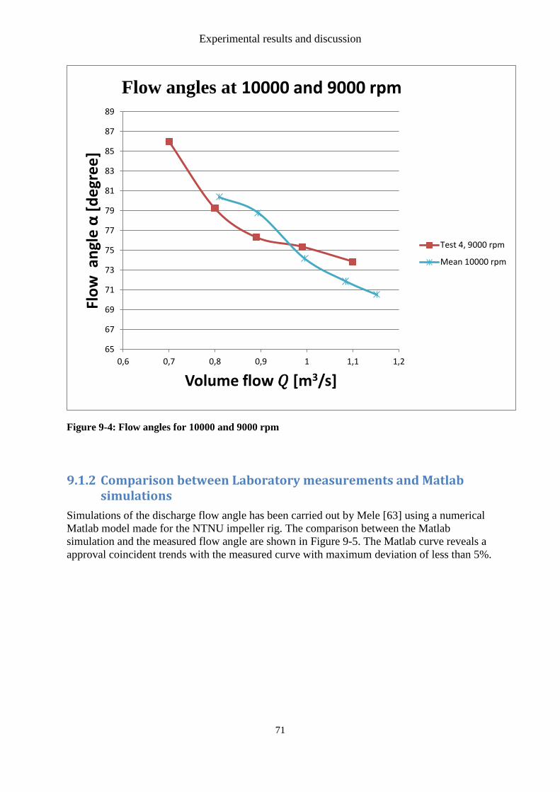
Experimental results and discussion
71
Figure 9-4: Flow angles for 10000 and 9000 rpm
9.1.2 Comparison between Laboratory measurements and Matlab simulations
Simulations of the discharge flow angle has been carried out by Mele [63] using a numerical
Matlab model made for the NTNU impeller rig. The comparison between the Matlab
simulation and the measured flow angle are shown in Figure 9-5. The Matlab curve reveals a
approval coincident trends with the measured curve with maximum deviation of less than 5%.
65
67
69
71
73
75
77
79
81
83
85
87
89
0,6 0,7 0,8 0,9 1 1,1 1,2
Flo
w a
ngl
e α
[d
egr
ee
]
Volume flow 𝑄 [m3/s]
Flow angles at 10000 and 9000 rpm
Test 4, 9000 rpm
Mean 10000 rpm
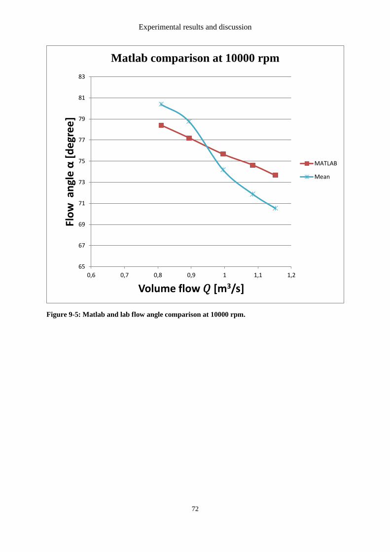
Experimental results and discussion
72
Figure 9-5: Matlab and lab flow angle comparison at 10000 rpm.
65
67
69
71
73
75
77
79
81
83
0,6 0,7 0,8 0,9 1 1,1 1,2
Flo
w a
ngl
e α
[d
egr
ee
]
Volume flow 𝑄 [m3/s]
Matlab comparison at 10000 rpm
MATLAB
Mean
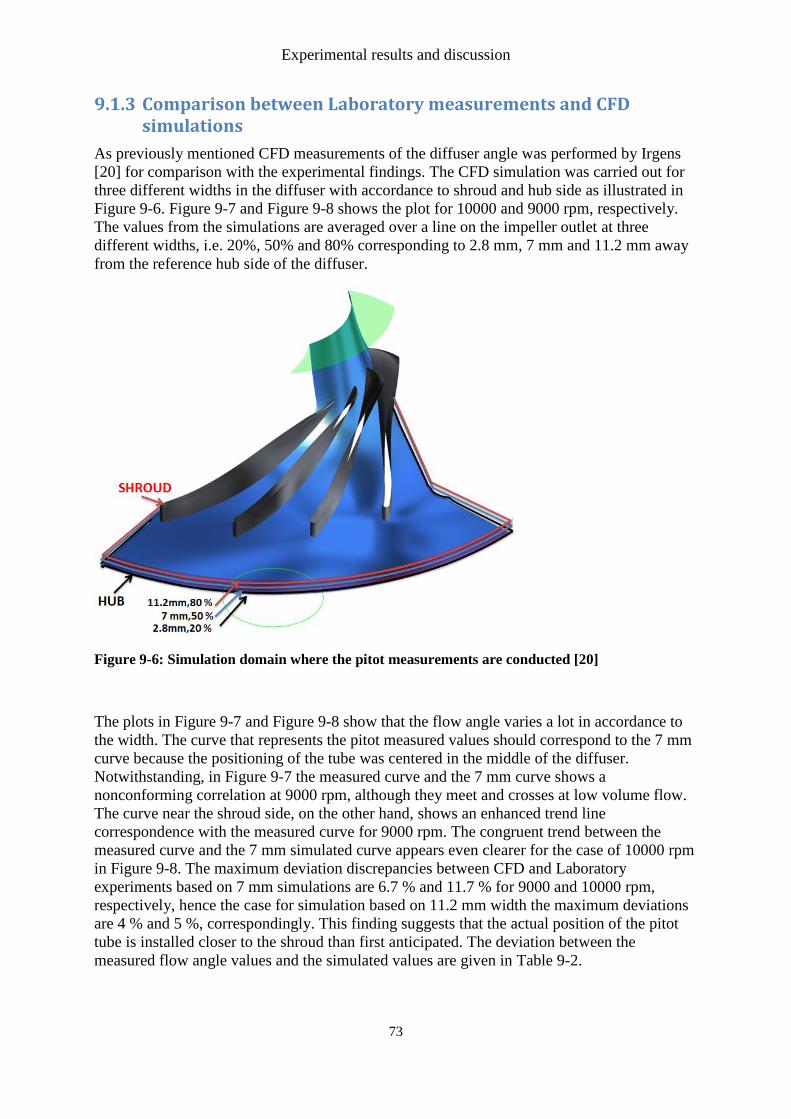
Experimental results and discussion
73
9.1.3 Comparison between Laboratory measurements and CFD simulations
As previously mentioned CFD measurements of the diffuser angle was performed by Irgens
[20] for comparison with the experimental findings. The CFD simulation was carried out for
three different widths in the diffuser with accordance to shroud and hub side as illustrated in
Figure 9-6. Figure 9-7 and Figure 9-8 shows the plot for 10000 and 9000 rpm, respectively.
The values from the simulations are averaged over a line on the impeller outlet at three
different widths, i.e. 20%, 50% and 80% corresponding to 2.8 mm, 7 mm and 11.2 mm away
from the reference hub side of the diffuser.
Figure 9-6: Simulation domain where the pitot measurements are conducted [20]
The plots in Figure 9-7 and Figure 9-8 show that the flow angle varies a lot in accordance to
the width. The curve that represents the pitot measured values should correspond to the 7 mm
curve because the positioning of the tube was centered in the middle of the diffuser.
Notwithstanding, in Figure 9-7 the measured curve and the 7 mm curve shows a
nonconforming correlation at 9000 rpm, although they meet and crosses at low volume flow.
The curve near the shroud side, on the other hand, shows an enhanced trend line
correspondence with the measured curve for 9000 rpm. The congruent trend between the
measured curve and the 7 mm simulated curve appears even clearer for the case of 10000 rpm
in Figure 9-8. The maximum deviation discrepancies between CFD and Laboratory
experiments based on 7 mm simulations are 6.7 % and 11.7 % for 9000 and 10000 rpm,
respectively, hence the case for simulation based on 11.2 mm width the maximum deviations
are 4 % and 5 %, correspondingly. This finding suggests that the actual position of the pitot
tube is installed closer to the shroud than first anticipated. The deviation between the
measured flow angle values and the simulated values are given in Table 9-2.
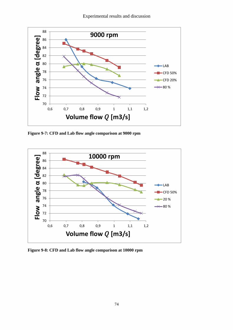
Experimental results and discussion
74
Figure 9-7: CFD and Lab flow angle comparison at 9000 rpm
Figure 9-8: CFD and Lab flow angle comparison at 10000 rpm
70
72
74
76
78
80
82
84
86
88
0,6 0,7 0,8 0,9 1 1,1 1,2
Flo
w a
ngl
e α
[d
egr
ee
]
Volume flow 𝑄 [m3/s]
9000 rpm
LAB
CFD 50%
CFD 20%
80 %
70
72
74
76
78
80
82
84
86
88
0,6 0,7 0,8 0,9 1 1,1 1,2
Flo
w a
ngl
e α
[d
egr
ee
]
Volume flow 𝑄 [m3/s]
10000 rpm
LAB
CFD 50%
20 %
80 %
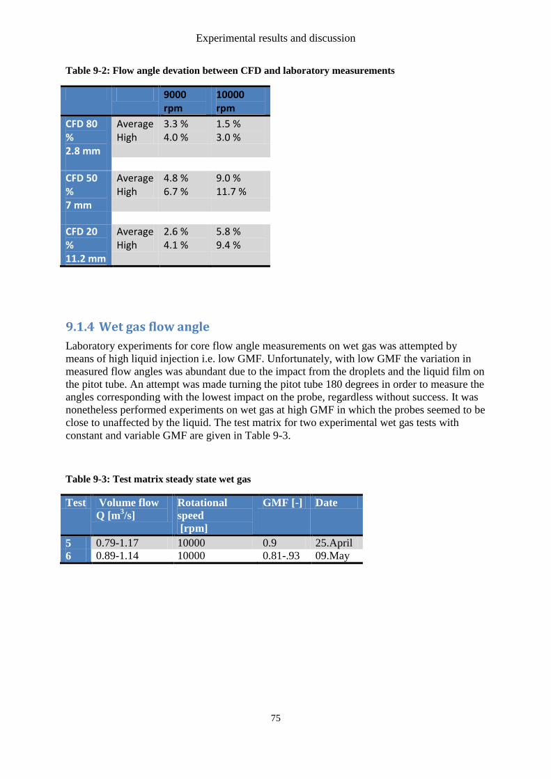
Experimental results and discussion
75
Table 9-2: Flow angle devation between CFD and laboratory measurements
9000 rpm
10000 rpm
CFD 80 % 2.8 mm
Average High
3.3 % 4.0 %
1.5 % 3.0 %
CFD 50 % 7 mm
Average High
4.8 % 6.7 %
9.0 % 11.7 %
CFD 20 % 11.2 mm
Average High
2.6 % 4.1 %
5.8 % 9.4 %
9.1.4 Wet gas flow angle
Laboratory experiments for core flow angle measurements on wet gas was attempted by
means of high liquid injection i.e. low GMF. Unfortunately, with low GMF the variation in
measured flow angles was abundant due to the impact from the droplets and the liquid film on
the pitot tube. An attempt was made turning the pitot tube 180 degrees in order to measure the
angles corresponding with the lowest impact on the probe, regardless without success. It was
nonetheless performed experiments on wet gas at high GMF in which the probes seemed to be
close to unaffected by the liquid. The test matrix for two experimental wet gas tests with
constant and variable GMF are given in Table 9-3.
Table 9-3: Test matrix steady state wet gas
Test Volume flow
Q [m3/s]
Rotational
speed
[rpm]
GMF [-] Date
5 0.79-1.17 10000 0.9 25.April
6 0.89-1.14 10000 0.81-.93 09.May
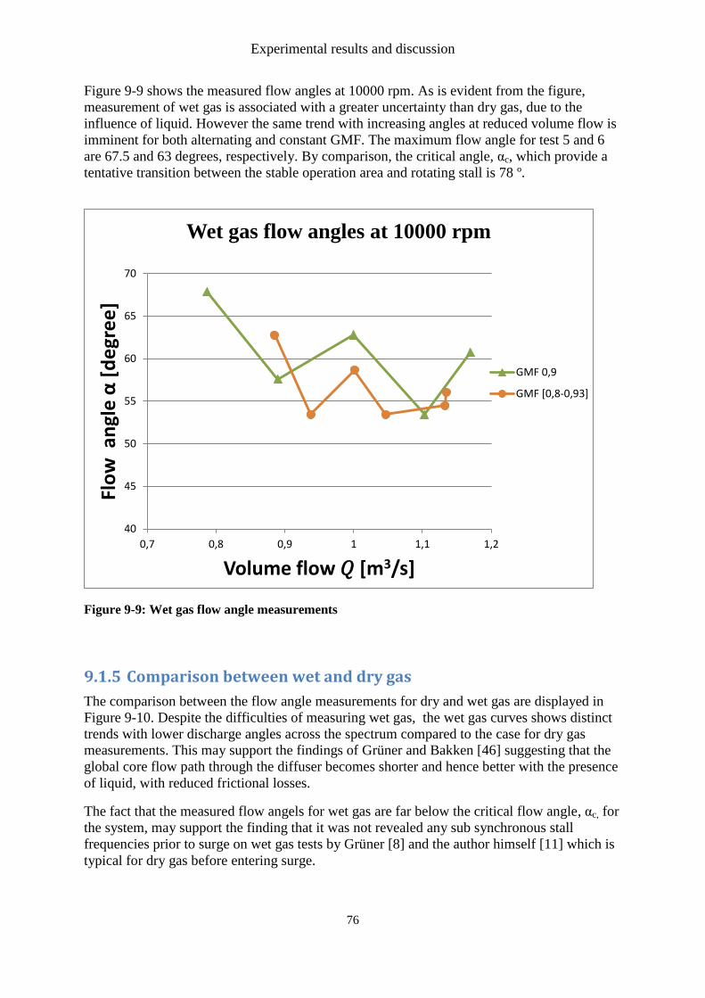
Experimental results and discussion
76
Figure 9-9 shows the measured flow angles at 10000 rpm. As is evident from the figure,
measurement of wet gas is associated with a greater uncertainty than dry gas, due to the
influence of liquid. However the same trend with increasing angles at reduced volume flow is
imminent for both alternating and constant GMF. The maximum flow angle for test 5 and 6
are 67.5 and 63 degrees, respectively. By comparison, the critical angle, αc, which provide a
tentative transition between the stable operation area and rotating stall is 78 º.
Figure 9-9: Wet gas flow angle measurements
9.1.5 Comparison between wet and dry gas
The comparison between the flow angle measurements for dry and wet gas are displayed in
Figure 9-10. Despite the difficulties of measuring wet gas, the wet gas curves shows distinct
trends with lower discharge angles across the spectrum compared to the case for dry gas
measurements. This may support the findings of Grüner and Bakken [46] suggesting that the
global core flow path through the diffuser becomes shorter and hence better with the presence
of liquid, with reduced frictional losses.
The fact that the measured flow angels for wet gas are far below the critical flow angle, αc, for
the system, may support the finding that it was not revealed any sub synchronous stall
frequencies prior to surge on wet gas tests by Grüner [8] and the author himself [11] which is
typical for dry gas before entering surge.
40
45
50
55
60
65
70
0,7 0,8 0,9 1 1,1 1,2
Flo
w a
ngl
e α
[d
egr
ee
]
Volume flow 𝑄 [m3/s]
Wet gas flow angles at 10000 rpm
GMF 0,9
GMF [0,8-0,93]
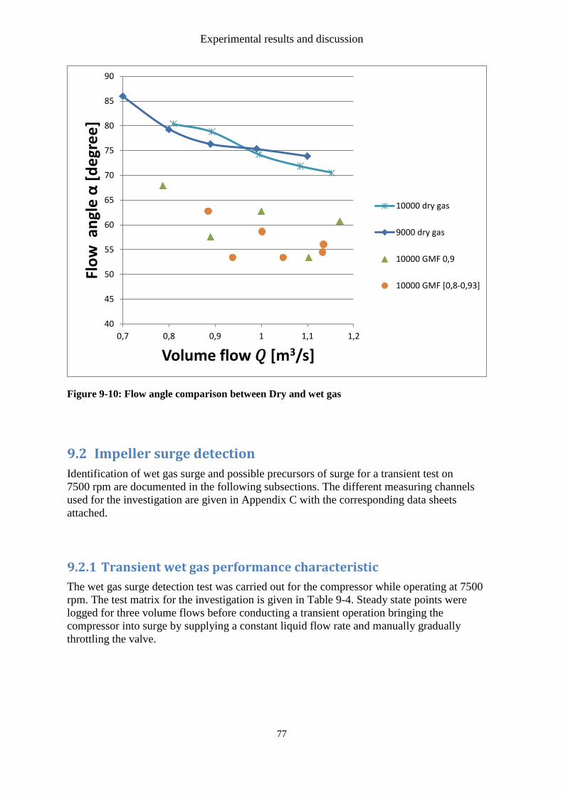
Experimental results and discussion
77
Figure 9-10: Flow angle comparison between Dry and wet gas
9.2 Impeller surge detection
Identification of wet gas surge and possible precursors of surge for a transient test on
7500 rpm are documented in the following subsections. The different measuring channels
used for the investigation are given in Appendix C with the corresponding data sheets
attached.
9.2.1 Transient wet gas performance characteristic
The wet gas surge detection test was carried out for the compressor while operating at 7500
rpm. The test matrix for the investigation is given in Table 9-4. Steady state points were
logged for three volume flows before conducting a transient operation bringing the
compressor into surge by supplying a constant liquid flow rate and manually gradually
throttling the valve.
40
45
50
55
60
65
70
75
80
85
90
0,7 0,8 0,9 1 1,1 1,2
Flo
w a
ngl
e α
[d
egr
ee
]
Volume flow 𝑄 [m3/s]
10000 dry gas
9000 dry gas
10000 GMF 0,9
10000 GMF [0,8-0,93]
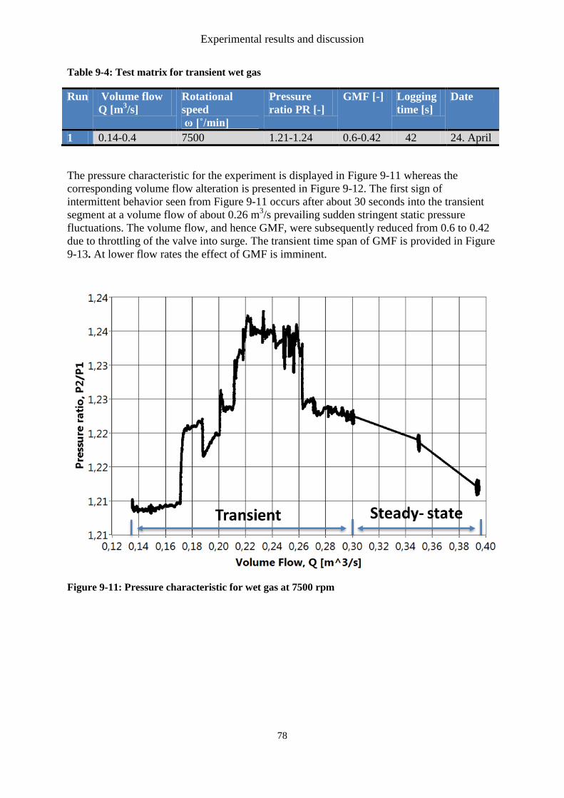
Experimental results and discussion
78
Table 9-4: Test matrix for transient wet gas
Run Volume flow
Q [m3/s]
Rotational
speed
ω [˚/min]
Pressure
ratio PR [-]
GMF [-] Logging
time [s]
Date
1 0.14-0.4 7500 1.21-1.24 0.6-0.42 42 24. April
The pressure characteristic for the experiment is displayed in Figure 9-11 whereas the
corresponding volume flow alteration is presented in Figure 9-12. The first sign of
intermittent behavior seen from Figure 9-11 occurs after about 30 seconds into the transient
segment at a volume flow of about 0.26 m3/s prevailing sudden stringent static pressure
fluctuations. The volume flow, and hence GMF, were subsequently reduced from 0.6 to 0.42
due to throttling of the valve into surge. The transient time span of GMF is provided in Figure
9-13. At lower flow rates the effect of GMF is imminent.
Figure 9-11: Pressure characteristic for wet gas at 7500 rpm
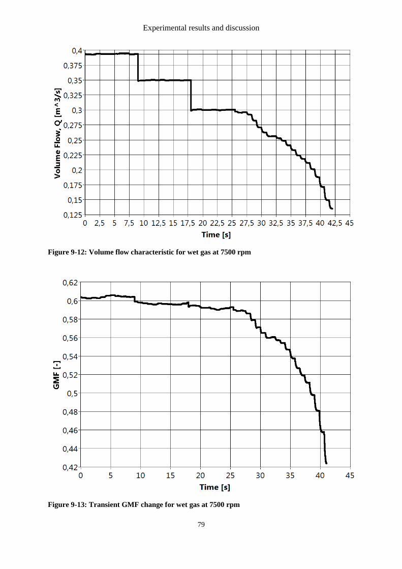
Experimental results and discussion
79
Figure 9-12: Volume flow characteristic for wet gas at 7500 rpm
Figure 9-13: Transient GMF change for wet gas at 7500 rpm
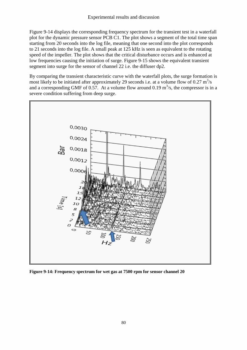
Experimental results and discussion
80
Figure 9-14 displays the corresponding frequency spectrum for the transient test in a waterfall
plot for the dynamic pressure sensor PCB C1. The plot shows a segment of the total time span
starting from 20 seconds into the log file, meaning that one second into the plot corresponds
to 21 seconds into the log file. A small peak at 125 kHz is seen as equivalent to the rotating
speed of the impeller. The plot shows that the critical disturbance occurs and is enhanced at
low frequencies causing the initiation of surge. Figure 9-15 shows the equivalent transient
segment into surge for the sensor of channel 22 i.e. the diffuser dp2.
By comparing the transient characteristic curve with the waterfall plots, the surge formation is
most likely to be initiated after approximately 29 seconds i.e. at a volume flow of 0.27 m3/s
and a corresponding GMF of 0.57. At a volume flow around 0.19 m3/s, the compressor is in a
severe condition suffering from deep surge.
Figure 9-14: Frequency spectrum for wet gas at 7500 rpm for sensor channel 20
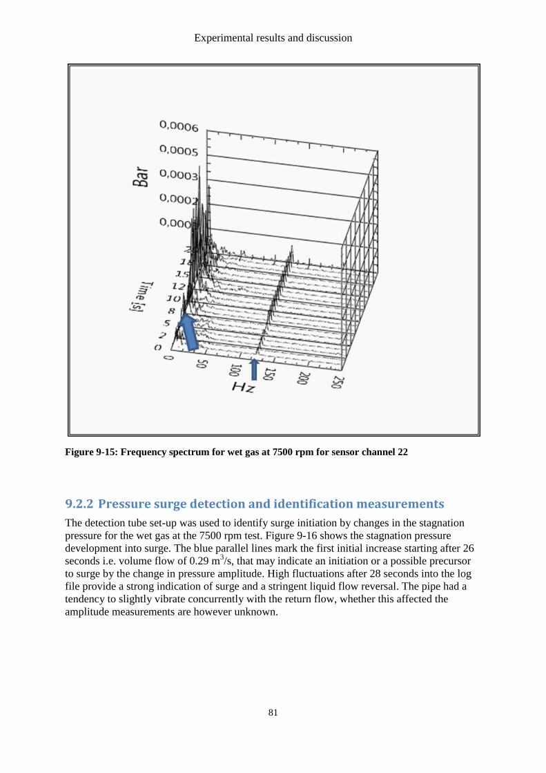
Experimental results and discussion
81
Figure 9-15: Frequency spectrum for wet gas at 7500 rpm for sensor channel 22
9.2.2 Pressure surge detection and identification measurements
The detection tube set-up was used to identify surge initiation by changes in the stagnation
pressure for the wet gas at the 7500 rpm test. Figure 9-16 shows the stagnation pressure
development into surge. The blue parallel lines mark the first initial increase starting after 26
seconds i.e. volume flow of 0.29 m3/s, that may indicate an initiation or a possible precursor
to surge by the change in pressure amplitude. High fluctuations after 28 seconds into the log
file provide a strong indication of surge and a stringent liquid flow reversal. The pipe had a
tendency to slightly vibrate concurrently with the return flow, whether this affected the
amplitude measurements are however unknown.
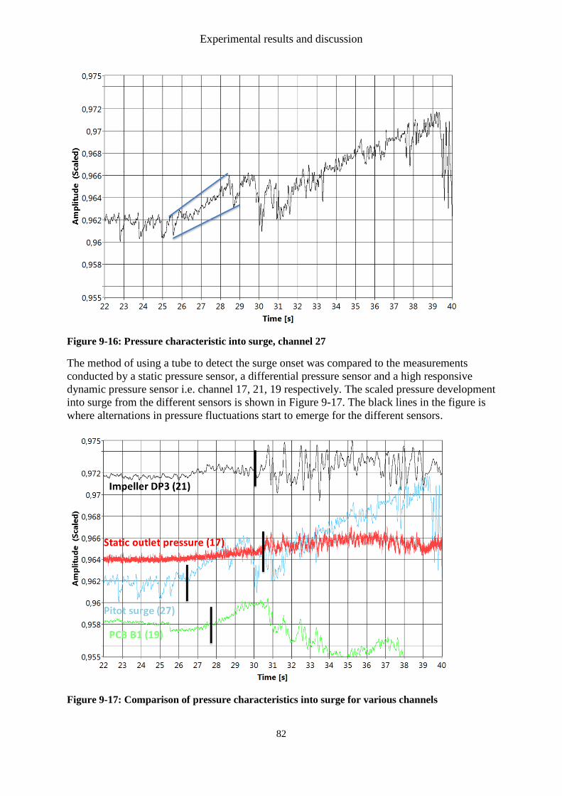
Experimental results and discussion
82
Figure 9-16: Pressure characteristic into surge, channel 27
The method of using a tube to detect the surge onset was compared to the measurements
conducted by a static pressure sensor, a differential pressure sensor and a high responsive
dynamic pressure sensor i.e. channel 17, 21, 19 respectively. The scaled pressure development
into surge from the different sensors is shown in Figure 9-17. The black lines in the figure is
where alternations in pressure fluctuations start to emerge for the different sensors.
Figure 9-17: Comparison of pressure characteristics into surge for various channels
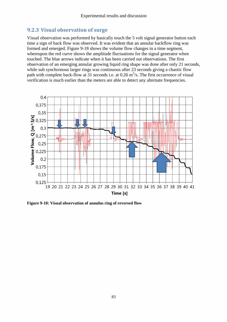
Experimental results and discussion
83
9.2.3 Visual observation of surge
Visual observation was performed by basically touch the 5 volt signal generator button each
time a sign of back flow was observed. It was evident that an annular backflow ring was
formed and emerged. Figure 9-18 shows the volume flow changes in a time segment,
whereupon the red curve shows the amplitude fluctuations for the signal generator when
touched. The blue arrows indicate when it has been carried out observations. The first
observation of an emerging annular growing liquid ring shape was done after only 21 seconds,
while sub synchronous larger rings was continuous after 23 seconds giving a chaotic flow
path with complete back-flow at 31 seconds i.e. at 0.26 m3/s. The first occurrence of visual
verification is much earlier than the meters are able to detect any alternate frequencies.
Figure 9-18: Visual observation of annulus ring of reversed flow

Experimental results and discussion
84
Discussion
85
10 Discussion
This chapter will serve as a discussion and conclusion for the results of the two main
experimental investigations performed in this master thesis.
Flow angle investigation
Flow angle experiments for dry gas were performed at 10000 and 9000 rpm steady state. The
flow angle increases with decreasing volume flow. The maximum flow angle conducted for
dry gas on 10000 rpm was 81.5 degrees. A sudden rise in flow angle gradient was found to
occur between volume flows close to 1 and 0.90 m3/s. As for 10000 rpm, the 9000 rpm curve
experiences a gradient rise, with decreasing volume flow, from 0.8 m3/s. This implies that the
same impact, related to the impeller and diffuser characteristics, yields for both 9000 rpm and
10000 rpm. Maximum flow angle 9000 rpm was found to be 86 degrees. The available
correlations used in the Matlab simulation gives a fairly accurate result with a deviation of
less than 5 %. Deviation between CFD and laboratory experiments based on 7 mm
simulations are 6.7 % and 11.7 % for 9000 and 10000 rpm, respectively, hence the case for
simulation based on 11.2 mm width the maximum deviations are 4 % and 5 %,
correspondingly.
This finding suggests that the actual position of the pitot tube is installed closer to the shroud
than first anticipated. Measurement of wet gas is associated with a greater uncertainty than
dry gas, due to the influence of liquid. However, the same trend with increasing angles at
reduced volume flow is imminent for both alternating and constant GMF. The maximum flow
angle for test 5 and 6 are 67.5 and 63 degrees, respectively. Despite the difficulties of
measuring wet gas, the wet gas curves shows distinct trends with lower discharge angles
across the spectrum compared to the case for dry gas measurements. This may support the
suggesting that the global core flow path through the diffuser becomes shorter and hence
better with the presence of liquid with reduced frictional losses.
Wet gas surge detection
The wet gas surge detection test was carried out for the compressor while operating at 7500
rpm. The first sign of intermittent behavior occurs after about 30 seconds into the transient
segment at a volume flow of about 0.26 m3/s prevailing sudden stringent static pressure
fluctuations. At lower flow rates the effect of GMF is imminent. By comparing the transient
characteristic curve with the waterfall plots the surge formation is most likely to be initiated
after approximately 29 seconds i.e. at a volume flow of 0.27 m3/s and a corresponding GMF
of 0.57. At a volume flow of roughly 0.19 m3/s, the compressor is in a severe condition
suffering from deep surge. A change in the stagnation pressure after 26 seconds might be a
possible indication of surge. The pipe had a tendency to slightly vibrate concurrently with the
return flow, whether this affected the amplitude measurements are however unknown. The
first observation of an emerging liquid ring shape was done after only 21 seconds, while sub
synchronous larger rings was continuous after 23 seconds giving a chaotic flow path with
complete back-flow at 31 seconds i.e. at 0.26 m3/s.

Discussion
86
1 Recommendations for further work
87
11 Recommendations for further work
This chapter will present advices for further work for the results of the two main experimental
investigations performed in this master thesis.
Flow angle investigation
The liquid may impact the flow velocity and direction by means of providing the flow with
momentum, and thereby change the global core flow path through the diffuser to a shorter and
hence better flow path with reduced frictional losses. Exact measuring of the wet gas flow
velocity angle is thereby of high importance providing higher insight into stability
considerations due to the presence of liquid.
The tests on dry gas flow angle measurements revealed higher angles with decreasing flow
rate with uncertainty based on the manual measurement method. More precise measurements
can be achieved by use of a configuration of multi-hole probes that provides a larger operation
area meaning that the tube does not need to be turned around in the measurement domain.
Flow test for wet gas turned out to be very uneven due to interference and blockage at
especially high GMF. By introduce a blow-out function or heating of the pitot tube one can
circumvent the problem of blocking. In addition other types of measurement methods should
be considered and examined. The development of sensors for wet gas flow may be required.
Identification of the liquid film flow will also be a major discovery for comparison. For both
the wet and dry gas tests is should be tested for a larger volume-flow range, preferably into
the very unstable area for different rpms. In addition since the the flow distribution is highly
uneven across the width of the diffuser, it is important to perform several measurements
across the full width to validate against for instance CFD simulation.
Wet gas surge detection
In the case of detection of surge it should be performed more repeatable tests at different
speeds and validate against the visually confirmation of back flow. Unfortunately the pipe that
was used for surge identification was not necessarily sufficient rigid. In addition the length of
the coupling tubing between the tube and the transmitter could have been shorter favor earlier
detection of the surge. It was conducted machining of two additional pipes with greater
diameter of 3mm and 6mm respectively. However, these were not tried out due to downtime
on the impeller rig because of inducer implementation on the impeller. The author
recommends that these tubes should be tested together with alternative methods to ensure
exact identification of instability inception. The author believes that the FRAP system with
built in detectors should be validated and tested for the purpose of identification of possibel
surge precursors.

1 Recommendations for further work

DiscussionReferences
References
1. Oljedirektoratet, PETROLEUMSRESSURSENE PÅ NORSK KONTINENTALSOKKEL. 2011. 2. STATOIL, 2011. 3. Bakken, T.G.G.a.L.E., AERODYNAMIC INSTABILITY INVESTIGATION OF A CENTRIFUGAL
COMPRESSOR EXPOSED TO WET GAS. Department of Energy and Process Engineering, Norwegian University of Science and Technology (NTNU), 2010: p. 12.
4. Hundseid, O., et al., Wet Gas Performance of a Single Stage Centrifugal Compressor. ASME Conference Proceedings, 2008(43178): p. 661-670.
5. Wood, A.B., A Textbook of Sound, ed. G.B.a.S. Ltd 1944, London. 6. Taitel Y., D.A.E., A Model For Predicting Flow Regime Transitions in Horizontal and
Near-Horizontal Gas-Liquid Flow. AIChE Journal, 1976. 22(1): p. 47-55. 7. Schubring, D. and T.A. Shedd, Critical friction factor modeling of horizontal annular
base film thickness. International Journal of Multiphase Flow, 2009. 35(4): p. 389-397.
8. Schlichting, H. and K. Gersten, Boundary-layer theory. 8th rev. and enl. ed 2000, Berlin ; New York: Springer. xxiii, 799 p.
9. C.Xu., R.S.A., The development of centrifugal compressor impeller. Proceedings of ASME Turbo Expo 2008:,.
10. Saravanamuttoo, H.I.H., Gas turbine theory. 6th ed2009, Harlow, England ; New York: Pearson Prentice Hall. xvi, 590 p.
11. Sørvik, L.A.Ø., Aerodynamic instabilities in a centrifugal compressor, in Department of Energy and Process Engineering2011, NTNU: Trondheim, Norway.
12. Cumpsty, N.A., Compressor aerodynamics1989, Harlow, Essex, England New York: Longman Scientific & Technical ; J. Wiley. 509 p.
13. Boyce, M.P., Gas turbine engineering handbook. 3rd ed2006, Boston: Gulf Professional Pub. xviii, 936 p.
14. Eckardt, D., Detailed Flow Investigations Within a High-Speed Centrifugal Compressor Impeller. Journal of Fluids Engineering, 1976. 98(3): p. 390-399.
15. Robert C. Dean, J. and Y. Senoo, Rotating Wakes in Vaneless Diffusers. Journal of Basic Engineering, 1960. 82(3): p. 563-570.
16. AhmadR.Ganji, A.J.W., Introduction to Engineering Experiments. Third Edition ed2010: Pearson.
17. Bryan, W.B., An investigation of unsteady impeller-diffuser interactions in a centrifugal compressor, in Mechanical engineering 1991, Purdue University: United States Indiana. p. 192.
18. Cumpsty, N.A., Compressor aerodynamics. 2nd ed 2004, Harlow, Essex, England New York: Krieger Pub Co.
19. O.Viseth, T., Optimalisering av våtgass diffusor og spiralhus, in Institutt for Energi- og Prosessteknikk 2012, NTNU: Trondheim, Norway.
20. J.Irgens, S., Optimailisering av løpehjul for våtgass, in Institutt for Energi- og Prosessteknikk 2012, NTNU: Trondheim, Norway.
21. Brenne, L., Straight -Walled Diffuser Performance: An experimental investigaion of the diffuser pressure recovery with single- phase airflow and two phase air- water annular flow, in Department of Energy and Prosess Engineering2004, The Norwegian University of Technology
22. C.Pampreen, R., Compressor Surge and Stall 1993.
DiscussionReferences
23. Gravdahl, J.T. and O. Egeland, Compressor surge and rotating stall : modelling and control. Advances in industrial control 1999, London ; New York: Springer. xix, 225 p.
24. Engeda, A., The unsteady performance of a centrifugal compressor with different diffusers. Proceedings of the Institution of Mechanical Engineers, Part A: Journal of Power and Energy, 2001. 215(5): p. 585-599.
25. G Ferrara , L.a.L.B., Rotating Stall in Centrifugal Compressor Vaneless Diffuser: Experimental Analysis of Geometrical Parameters Influence on Phenomenon Evolution. International Journal of Rotating Machinery, 2004. 10(6): p. 433–442.
26. Brillhart, J., Rotating stall in centrifugal compressors. 2009. 27. Jansen, W., Rotating stall in a radial vaneless diffuser. ASME, 1964. 28. Senoo, Y. and Y. Kinoshita, Influence of Inlet Flow Conditions and Geometries of
Centrifugal Vaneless Diffusers on Critical Flow Angle for Reverse Flow. Journal of Fluids Engineering, 1977. 99(1): p. 98-102.
29. Baines, A.W.a.N.C., Design of Radial Turbomachines, ed. P. Education1990, New York: Pearson Education Longman Scientific & Technical. 414.
30. Yasutoshi Senoo, Y.K., Limits in rotating stall and stall in vaneless diffusers of centrifugal compressors, in ASME paper 78-GT- 191978.
31. Abdelhamid, A.N., Analysis of rotating stall in vaneless diffusers of centrifugal compressors. ASME paper 80-GT- 184, 1980.
32. Frigne, P., Van Den Braembusche,R, Distinction between different types of impeller and diffuser rotating stall in a centrifugal compressor with vaneless diffuser. ASME paper 83-GT-61, 1983.
33. Jager, B.d., Rotating stall and surge control: A survey. Proceedings of the 34th Conference on Decision & Control, 1995.
34. Greitzer, E.M., Surge and Rotating Stall in Axial Flow Compressors---Part I: Theoretical Compression System Model. Journal of Engineering for Power, 1976. 98(2): p. 190-198.
35. Fink, D.A., N.A. Cumpsty, and E.M. Greitzer, Surge Dynamics in a Free-Spool Centrifugal Compressor System. Journal of Turbomachinery, 1992. 114(2): p. 321-332.
36. Hartel, C. and P. Pfeiffer, Model Analysis of High-Fogging Effects on the Work of Compression. ASME Conference Proceedings,. 2003(36851): p. 689-698.
37. Wang, Y., et al., Analysis of Effects on Wet Compression on Surge Margin of a Small Gas Turbine. ASME Conference Proceedings,. 2002(36177): p. 247-252.
38. Day, I., J. Williams, and C. Freeman, Rain Ingestion in Axial Flow Compressors at Part Speed. ASME Conference Proceedings,. 2005(47306): p. 223-235.
39. Abdelwahab, A., An Investigation of the Use of Wet Compression in Industrial Centrifugal Compressors. ASME Conference Proceedings,. 2006(42398): p. 741-750.
40. L. Brenne, T.B., Josè l.Gilarranz, Jay M. Koch and Harry Miller, Performance evaluation of a centrifugal compressor operating under wet gas conditions, in In Proceedings of the Thirty-Fourth Turbomachinery Symposium2005: Houston, Texas, USA. p. 10.
41. Gruner, T.G., et al., An Experimental Investigation of Airfoil Performance in Wet Gas Flow. ASME Conference Proceedings, 2008. 2008(43178): p. 575-584.
42. Fabbrizzi, M., et al., An Experimental Investigation of a Single Stage Wet Gas Centrifugal Compressor. ASME Conference Proceedings,. 2009(48869): p. 443-453.
43. Bigi, D.R.L.P.M.W.M.B.a.M., Mechanical Performance of a Two Stage Centrifugal Compressor under Wet Gas Conditions. Proceedings of the Fortieth Turbomachinery Symposium September 12-15, 2011, Houston, Texas, 2011.

DiscussionReferences
44. Bakken, T.G.G.a.L.E. INSTABILITY CHARACTERISTIC OF A SINGLE-STAGE CENTRIFFUGAL COMPRESSOR EXPOSED TO DRY AND WET GAS. in Proceedings of ASME Turbo Expo 2012: Power Land, Sea and Air June 11-15 2012. Copenhagen , Denmark.
45. Crane, R.I.M., M. J, Interpretation of pitot pressure in compressible two-phase flow. J. Mech. Engng Sci., 1972. 14: p. 128-133.
46. Grüner.T., a.B., L.E.,, Instability Characteristic of a Single-Stage Centrifugal Compressor Exposed to Dry and Wet gas. ASME Turbo Expo 2012: Power for Land, Sea And Air June 11-15 Copenhagen, Denmark, 2012(GT2012-69473).
47. Grüner, T.G., Wet Gas Compression: Experimental investigation of the aerodynamics within a centrifugal compressor exposed for wet gas, in Faculty of Engineering Science and Process Engineering Department of Energy and Process Engineering2012, NTNU Norwegian University of Science and Technology: Trondheim
48. C. Bertani, M.D.S., M. Malandrone, G. Monni and B. Panella, State-of-Art and selection of techniques in multiphase flow measurement, l.E.e.l.S.E.S. Agenzia Nazionale per le Nuove Tecnologie, Editor, POLITECNICO’ DI TORINO DIPARTIMENTO DI ENERGETICA: Torino, Luglio 2010.
49. Falcone, G.H., G.F and Alimonti, C, Multiphase flow metering :principles and applications. Developments in Petroleum science, ed. Elsevier. Vol. 54. 2010, Great Britain: Elsevier. 329.
50. Ziegler, K.U., H.E. Gallus, and R. Niehuis, A Study on Impeller-Diffuser Interaction---Part I: Influence on the Performance. Journal of Turbomachinery, 2003. 125(1): p. 173-182.
51. Ziegler, K.U., H.E. Gallus, and R. Niehuis, A Study on Impeller-Diffuser Interaction---Part II: Detailed Flow Analysis. Journal of Turbomachinery, 2003. 125(1): p. 183-192.
52. Gill, L.E., Sampling probe studies of the gas core in annular two-phase flow. Chem. Eng. Sci, 1963. 18(8): p. 525–535.
53. White, A.J., Young, J. B. & Walters, Experimental validation of condensing flow theory for a stationary cascade of steam turbine blades. Phil. Trans. R. Soc. Lond, 1996. A 354: p. 354.
54. Kupferschmied, P., et al., On the Development and Application of the Fast-Response Aerodynamic Probe System in Turbomachines---Part 1: The Measurement System. Journal of Turbomachinery, 2000. 122(3): p. 505-516.
55. Roduner, C., et al., On the Development and Application of the Fast-Response Aerodynamic Probe System in Turbomachines---Part 2: Flow, Surge, and Stall in a Centrifugal Compressor. Journal of Turbomachinery, 2000. 122(3): p. 517-526.
56. Schlienger, J., et al., Effects of Labyrinth Seal Variation on Multistage Axial Turbine Flow. ASME Conference Proceedings,. 2003(36894): p. 173-185.
57. Porreca, L., Hollenstein, M., Kalfas, A. I., and Abhari R. S.,, Turbulence Measurements and Analysis in a Multistage Axial Turbine. Journal of Propulsion and Power, 2007. 23(1): p. 227-234.
58. Christian, L., High Temperature Fast Response Aerodynamic Probe, 2010, ETH ZURICH: Zurich.
59. Schleer, M., et al., Investigation of an Inversely Designed Centrifugal Compressor Stage---Part II: Experimental Investigations. Journal of Turbomachinery, 2004. 126(1): p. 82-90.

DiscussionReferences
60. Zangeneh, M., et al., Investigation of an Inversely Designed Centrifugal Compressor Stage---Part I: Design and Numerical Verification. Journal of Turbomachinery, 2004. 126(1): p. 73-81.
61. Hazby, H.R., L. Xu, and M. Schleer, Study of the Flow in a Vaneless Diffuser at Part Speed Operating Conditions. ASME Conference Proceedings,. 2010(44021): p. 1913-1923.
62. Reitan, D.R., Validation of Wet Gas Performance, in Department of Energy and Process Engineering2012, NTNU: Trondheim, Norway.
63. Mele, E., Wet Gas Compressor Performance, in Department of Energy and Process Engineering2012, NTNU: Trondheim, Norway.
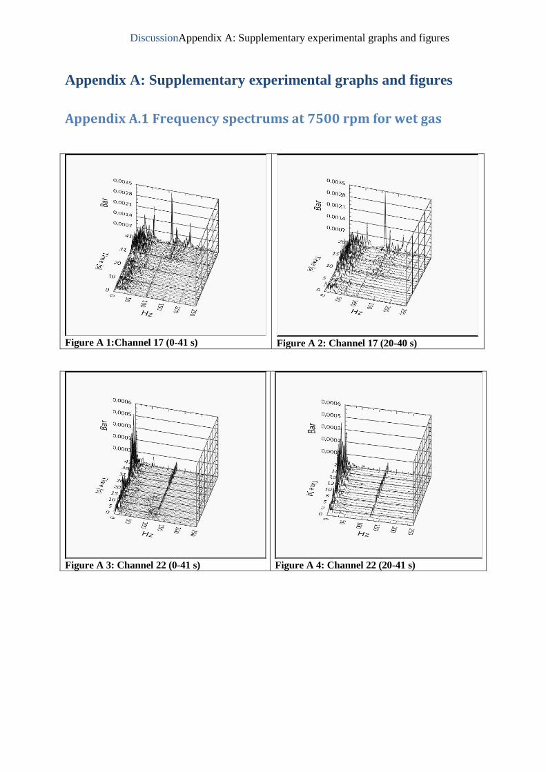
DiscussionAppendix A: Supplementary experimental graphs and figures
Appendix A: Supplementary experimental graphs and figures
Appendix A.1 Frequency spectrums at 7500 rpm for wet gas
Figure A 1:Channel 17 (0-41 s)
Figure A 2: Channel 17 (20-40 s)
Figure A 3: Channel 22 (0-41 s)
Figure A 4: Channel 22 (20-41 s)
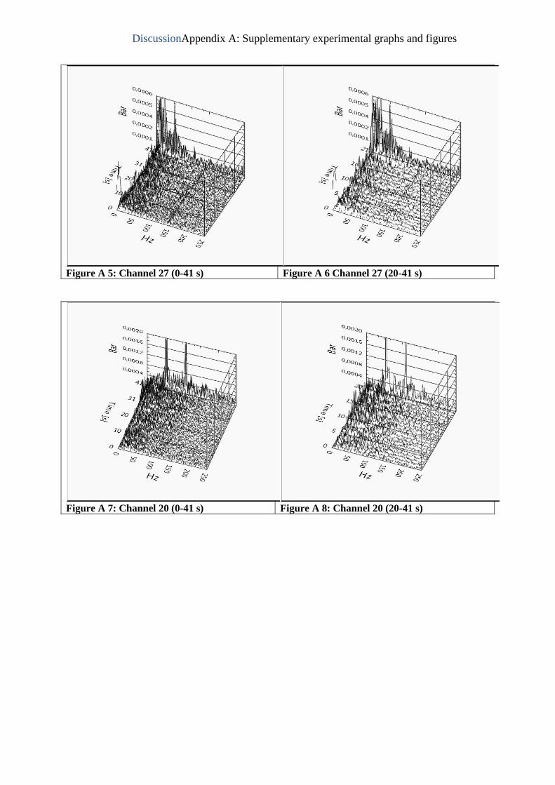
DiscussionAppendix A: Supplementary experimental graphs and figures
Figure A 5: Channel 27 (0-41 s)
Figure A 6 Channel 27 (20-41 s)
Figure A 7: Channel 20 (0-41 s)
Figure A 8: Channel 20 (20-41 s)
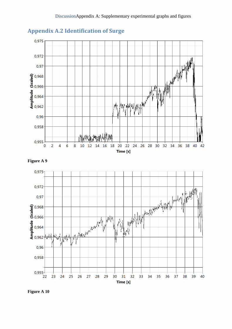
DiscussionAppendix A: Supplementary experimental graphs and figures
Appendix A.2 Identification of Surge
Figure A 9
Figure A 10
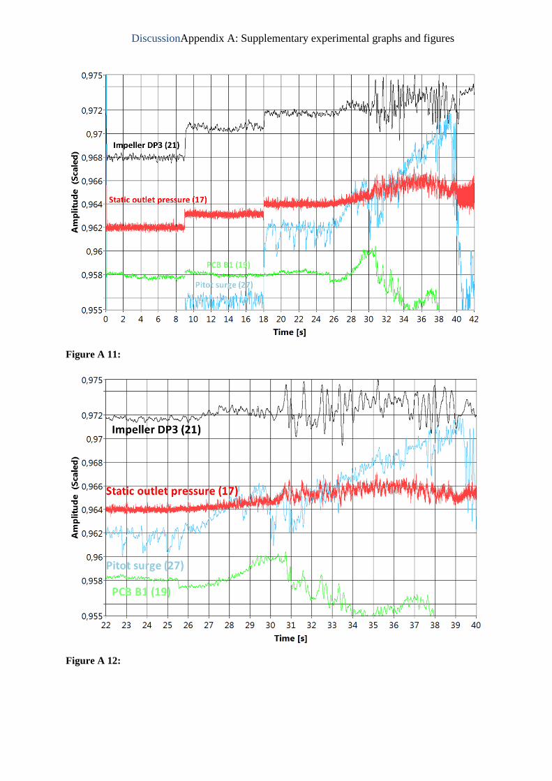
DiscussionAppendix A: Supplementary experimental graphs and figures
Figure A 11:
Figure A 12:
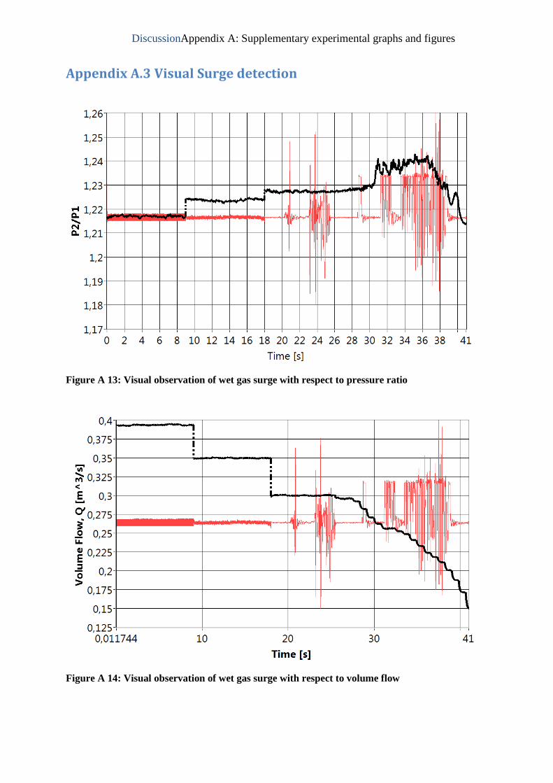
DiscussionAppendix A: Supplementary experimental graphs and figures
Appendix A.3 Visual Surge detection
Figure A 13: Visual observation of wet gas surge with respect to pressure ratio
Figure A 14: Visual observation of wet gas surge with respect to volume flow

Appendix B: Technical drawings of the impeller rig
Appendix B: Technical drawings of the impeller rig
Appendix B includes technical drawings made with the CAD software Autodesk Inventor
Professional describing the installation of pitot tubes inside the NTNU impeller rig. The
impeller is unfortunately not included in the drawing because the impeller contains
confidential geometries.
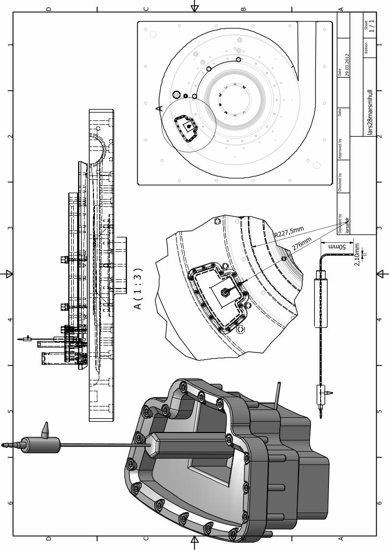
A ( 1 : 3 )
A
1 1
2 2
3 3
4 4
5 5
6 6
AA
BB
CC
DD
lars28m
arsm
hull
larsandr
29.03.2012
Designed by
Checked by
Approved by
Date
1 / 1
Edition
Sheet
Date
2,10m
m
50mm
2
7
6
m
m
R
2
2
7
,
5
m
m
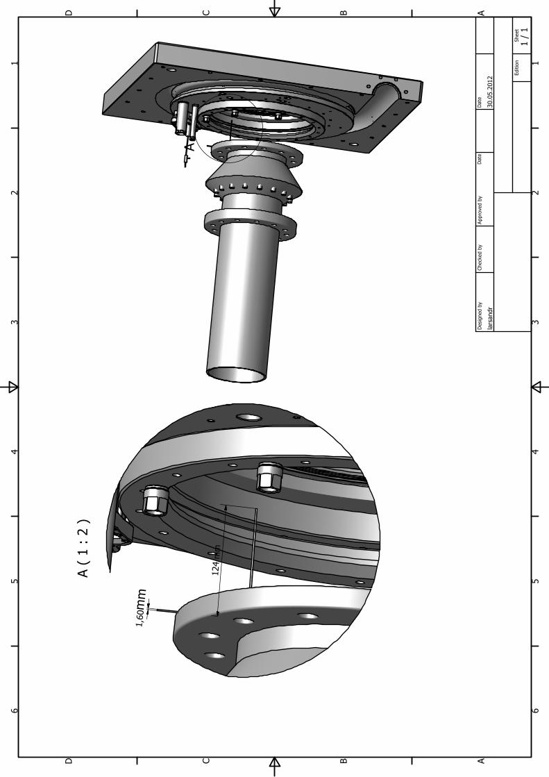
A ( 1 : 2 )
A
1 1
2 2
3 3
4 4
5 5
6 6
AA
BB
CC
DD
larsandr
30.05.2012
Designed by
Checked by
Approved by
Date
1 / 1
Edition
Sheet
Date
1
,6
0m
m
124 m
m

Appendix C: Instrumentation data sheets
Appendix C: Instrumentation data sheets
Appendix C is intended to give the reader an overview of the different measuring channels
that has been used for the execution of the tests. Data sheets of the main instrumentations
from the channel list below are included in Appendix C.2
Table C-1: NTNU Impeller channel list
Channel Description Unit
0 5 Volts signal generator bar
1 PCB B2 bar
5 P 3_1 dp volume flow mbar
6 P 10_1 Pressure inlet p1 bar
7 P 11_1 Compressor dp bar
8 T 5 1 Inlet Temperature T1 C
10 5 Volts signal generator Nm
12 Turbin Flow meter m3/s
13 P 3 3 Turbine pressure bar
16 P 3 4 static inlet pressure bar
17 P 3 5 static outlet pressure bar
18 PCB 32822 A bar
19 PCB 32845 B bar
20 PCB 32844 C bar
21 dp1 (Impeller) bar
22 dp2 (Diffuser) bar
23 dp3 (Volute) bar
24 DP4 (Pitot diffuser pitot tube ) mbar
27 P12-2 bar
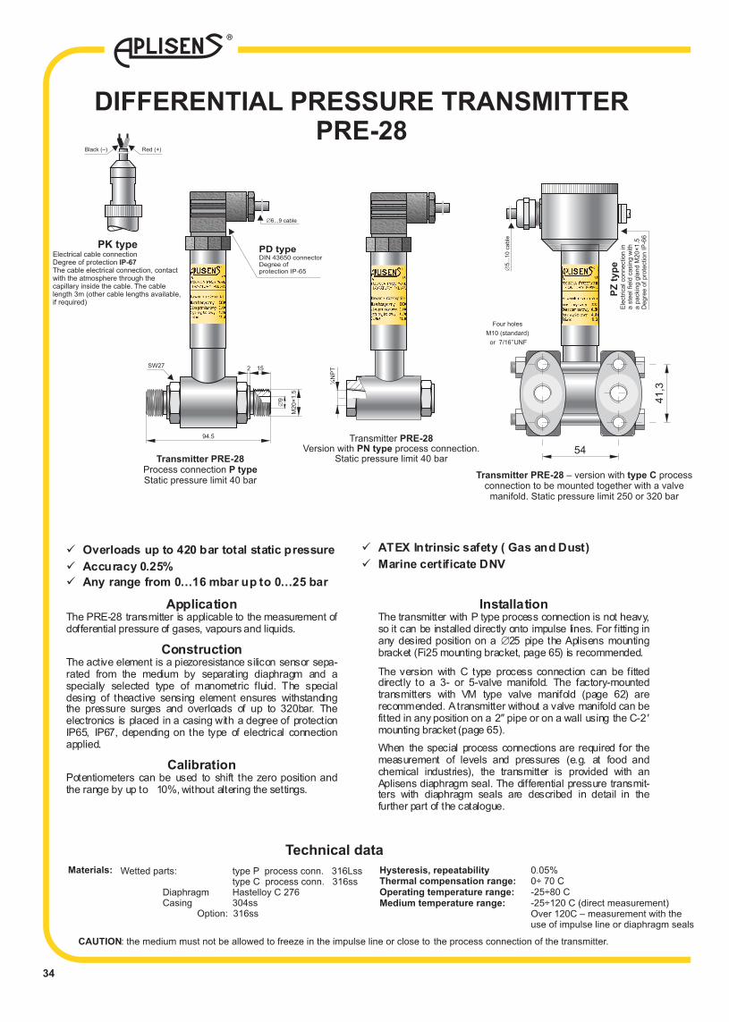
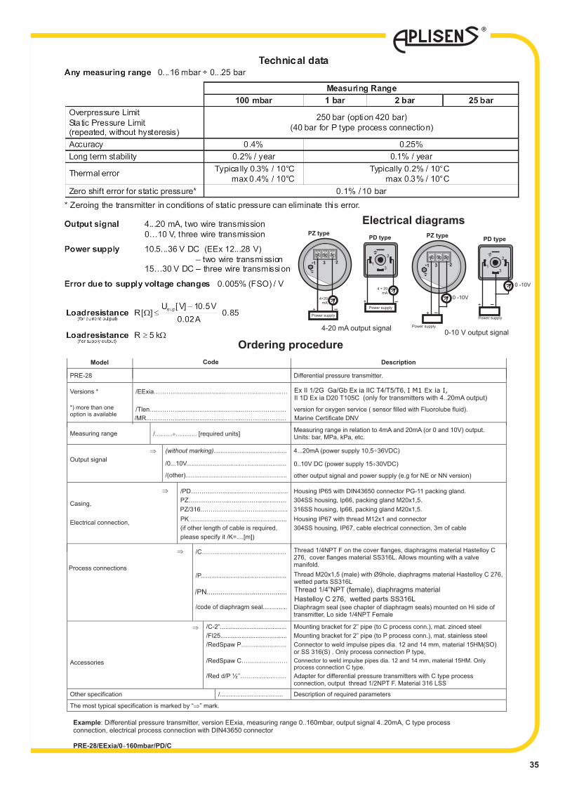
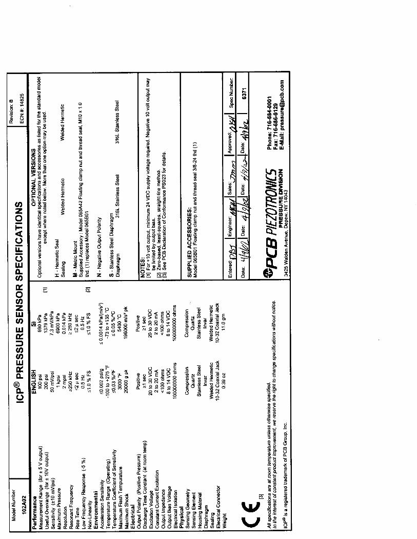
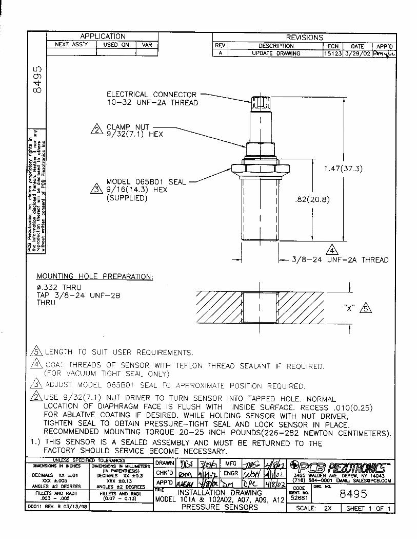

UNIK 5000
The UNIK 5000 is a high performance confi gurable solution to pressure measurement. The use of Druck silicon technology and analogue circuitry enables best in class performance for stability, low power and frequency response. The use of modular design and lean manufacturing techniques allow users to design the product required to their unique application requirements and for them to be delivered inside standard product lead times.
Features
• Ranges from 70 mbar (1.5 psi) to 700 bar (10,000 psi)
• Accuracy to ±0.04% Full Scale (FS) Best Straight Line (BSL)
• Stainless Steel construction
• Hazardous Area certifi cations (Pending)
• mV, mA, voltage and confi gurable voltage outputs.
• Multiple electrical connector options
Pressure Sensing Platform
GESensing & Inspection Technologies
• Multiple pressure connector options
• Operating temperature ranges to –55 to 125 °C
• Frequency response to 5 kHz
• High reliability
• High stability
• High over pressure capability
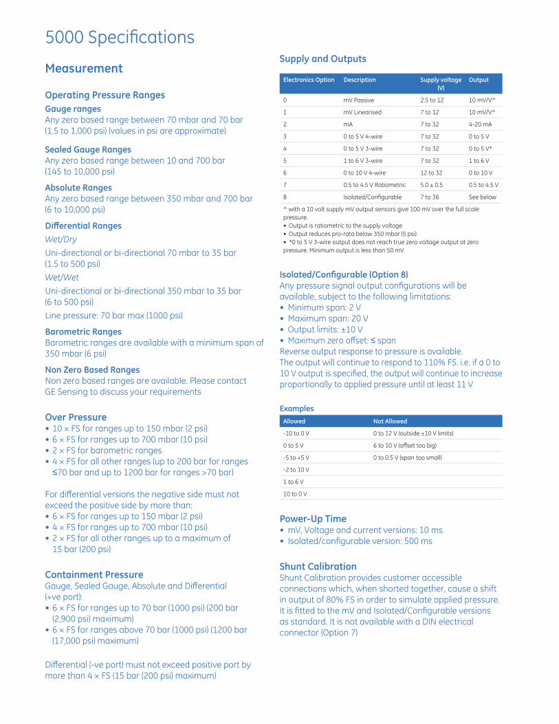
5000 Specifi cations
Measurement
Operating Pressure RangesGauge rangesAny zero based range between 70 mbar and 70 bar (1.5 to 1,000 psi) (values in psi are approximate)
Sealed Gauge RangesAny zero based range between 10 and 700 bar (145 to 10,000 psi)
Absolute RangesAny zero based range between 350 mbar and 700 bar (6 to 10,000 psi)
Diff erential RangesWet/Dry
Uni-directional or bi-directional 70 mbar to 35 bar (1.5 to 500 psi)Wet/Wet
Uni-directional or bi-directional 350 mbar to 35 bar (6 to 500 psi)Line pressure: 70 bar max (1000 psi)
Barometric RangesBarometric ranges are available with a minimum span of 350 mbar (6 psi)
Non Zero Based Ranges Non zero based ranges are available. Please contact GE Sensing to discuss your requirements
Over Pressure• 10 × FS for ranges up to 150 mbar (2 psi)• 6 × FS for ranges up to 700 mbar (10 psi)• 2 × FS for barometric ranges• 4 × FS for all other ranges (up to 200 bar for ranges ≤70 bar and up to 1200 bar for ranges >70 bar)
For diff erential versions the negative side must not exceed the positive side by more than:• 6 × FS for ranges up to 150 mbar (2 psi)• 4 × FS for ranges up to 700 mbar (10 psi)• 2 × FS for all other ranges up to a maximum of
15 bar (200 psi)
Containment PressureGauge, Sealed Gauge, Absolute and Diff erential (+ve port):• 6 × FS for ranges up to 70 bar (1000 psi) (200 bar
(2,900 psi) maximum)• 6 × FS for ranges above 70 bar (1000 psi) (1200 bar
(17,000 psi) maximum)
Diff erential (-ve port) must not exceed positive port by more than 4 × FS (15 bar (200 psi) maximum)
Supply and Outputs
Electronics Option Description Supply voltage(V)
Output
0 mV Passive 2.5 to 12 10 mV/V^
1 mV Linearised 7 to 12 10 mV/V^
2 mA 7 to 32 4-20 mA
3 0 to 5 V 4-wire 7 to 32 0 to 5 V
4 0 to 5 V 3-wire 7 to 32 0 to 5 V*
5 1 to 6 V 3-wire 7 to 32 1 to 6 V
6 0 to 10 V 4-wire 12 to 32 0 to 10 V
7 0.5 to 4.5 V Ratiometric 5.0 ± 0.5 0.5 to 4.5 V
8 Isolated/Confi gurable 7 to 36 See below
^ with a 10 volt supply mV output sensors give 100 mV over the full scale pressure. • Output is ratiometric to the supply voltage • Output reduces pro-rata below 350 mbar (5 psi)• *0 to 5 V 3-wire output does not reach true zero voltage output at zero pressure. Minimum output is less than 50 mV
Isolated/Confi gurable (Option 8)Any pressure signal output confi gurations will be available, subject to the following limitations:• Minimum span: 2 V• Maximum span: 20 V• Output limits: ±10 V• Maximum zero off set: ≤ spanReverse output response to pressure is available.The output will continue to respond to 110% FS. i.e. if a 0 to 10 V output is specifi ed, the output will continue to increase proportionally to applied pressure until at least 11 V
ExamplesAllowed Not Allowed
-10 to 0 V 0 to 12 V (outside ±10 V limits)
0 to 5 V 6 to 10 V (off set too big)
-5 to +5 V 0 to 0.5 V (span too small)
-2 to 10 V
1 to 6 V
10 to 0 V
Power-Up Time• mV, Voltage and current versions: 10 ms • Isolated/confi gurable version: 500 ms
Shunt CalibrationShunt Calibration provides customer accessible connections which, when shorted together, cause a shift in output of 80% FS in order to simulate applied pressure.It is fi tted to the mV and Isolated/Confi gurable versions as standard. It is not available with a DIN electrical connector (Option 7)
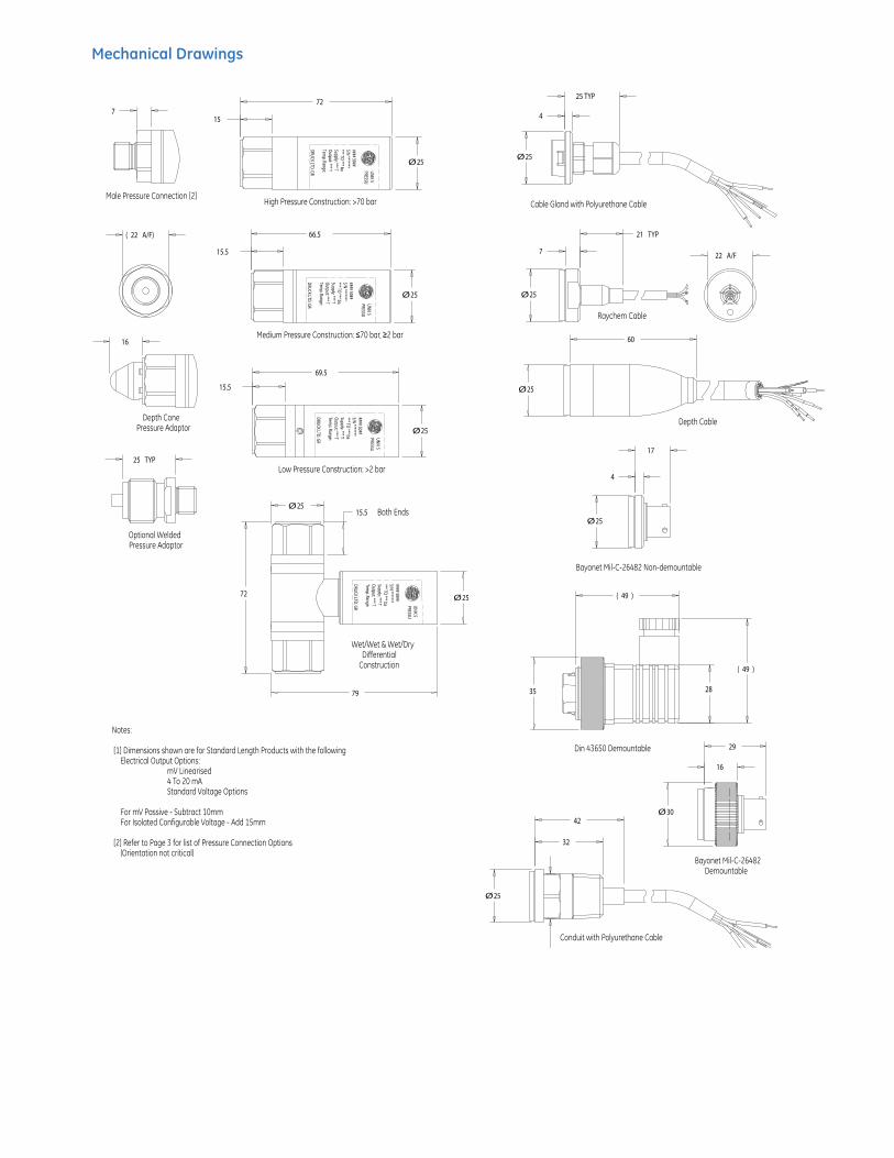
Mechanical Drawings
( A/F)22
7
TYP25
16
Notes:
[1] Dimensions shown are for Standard Length Products with the following Electrical Output Options: mV Linearised 4 To 20 mA Standard Voltage Options
For mV Passive - Subtract 10mm For Isolated Configurable Voltage - Add 15mm
[2] Refer to Page 3 for list of Pressure Connection Options (Orientation not critical)
Male Pressure Connection [2]
Optional WeldedPressure Adaptor
Depth ConePressure Adaptor
66.5
15.5
Ø25
UNIK 5 PRESSU
#### 50##S/N ********** TO
*** baSupply: *** TO
utput: *** TTem
p. Range:
DRUCK LTD. GR
69.5
15.5
Ø25
UNIK 5 PRESSU
#### 50##S/N ********** TO
*** baSupply: *** TO
utput: *** TTem
p. Range:
DRUCK LTD. GR
Ø25
72 Ø25
79
Both Ends15.5
Wet/Wet & Wet/DryDifferential
Construction
UNIK 5 PRESSU
#### 50##S/N ********** TO
*** baSupply: *** TO
utput: *** TTem
p. Range:
DRUCK LTD. GR
72
15
Ø25
High Pressure Construction: >70 bar
Low Pressure Construction: >2 bar
Medium Pressure Construction: ≤70 bar, ≥2 bar
UNIK 5 PRESSU
#### 50##S/N ********** TO
*** baSupply: *** TO
utput: *** TTem
p. Range:
DRUCK LTD. GR
25 TYP
Ø25
4
Cable Gland with Polyurethane Cable
7
Ø25
A/F22
TYP21
Raychem Cable
60
Ø25
Depth Cable
17
4
Ø25
Bayonet Mil-C-26482 Non-demountable
( )49
( )49
2835
Din 43650 Demountable 29
16
Ø30
Bayonet Mil-C-26482Demountable
32
42
Ø25
Conduit with Polyurethane Cable

ABILITYABILITY
HART®
I VE GOTI VE GOT,
FIELD COMMUNICATIONS PROTOCOL
SeriesSeriesSeries
• ± 0.04% High Accuracy
• ± 0.2% of URL Stability
Guarantee for 12 Years
• 120:1 Rangeability
• Non-volatile Flow Totalizer
• Tank Linearization
• 100 ms Total Response Time
• PID Control Capability
• Bi-directional Flow
Measurement
• Advanced Diagnostics
• Largest Library of Function
Block Execution Capacity
• Instantiable Function Blocks
• Supported by DD, EDDL
and FDT/DTM
• Three Technology Options
OCP-0007OCP-0007
R
MAXBBG Prüf- und Zertifizier GmbH
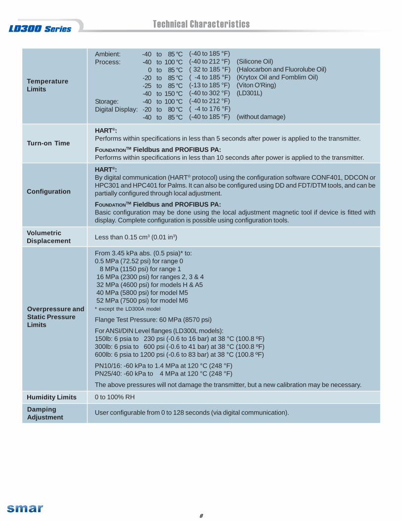
8
HART®:By digital communication (HART® protocol) using the configuration software CONF401, DDCON orHPC301 and HPC401 for Palms. It can also be configured using DD and FDT/DTM tools, and can bepartially configured through local adjustment.
FOUNDATIONTM Fieldbus and PROFIBUS PA:Basic configuration may be done using the local adjustment magnetic tool if device is fitted withdisplay. Complete configuration is possible using configuration tools.
VolumetricDisplacement Less than 0.15 cm3 (0.01 in3)
From 3.45 kPa abs. (0.5 psia)* to:0.5 MPa (72.52 psi) for range 0 8 MPa (1150 psi) for range 1 16 MPa (2300 psi) for ranges 2, 3 & 4 32 MPa (4600 psi) for models H & A5 40 MPa (5800 psi) for model M5 52 MPa (7500 psi) for model M6* except the LD300A model
Flange Test Pressure: 60 MPa (8570 psi)
For ANSI/DIN Level flanges (LD300L models):150lb: 6 psia to 230 psi (-0.6 to 16 bar) at 38 °C (100.8 ºF)300lb: 6 psia to 600 psi (-0.6 to 41 bar) at 38 °C (100.8 ºF)600lb: 6 psia to 1200 psi (-0.6 to 83 bar) at 38 °C (100.8 ºF)
PN10/16: -60 kPa to 1.4 MPa at 120 °C (248 °F)PN25/40: -60 kPa to 4 MPa at 120 °C (248 °F)
The above pressures will not damage the transmitter, but a new calibration may be necessary.
Technical Characteristics
Configuration
Humidity Limits 0 to 100% RH
Overpressure andStatic PressureLimits
User configurable from 0 to 128 seconds (via digital communication).DampingAdjustment
TemperatureLimits
Ambient:Process:
Storage:Digital Display:
-40-40
0-20-25-40-40-20-40
85100858585
1501008085
tototototototototo
(-40 to 185 °F)(-40 to 212 °F) (Silicone Oil)( 32 to 185 °F) (Halocarbon and Fluorolube Oil)( -4 to 185 °F) (Krytox Oil and Fomblim Oil)(-13 to 185 °F) (Viton O'Ring)(-40 to 302 °F) (LD301L)(-40 to 212 °F)( -4 to 176 °F)(-40 to 185 °F) (without damage)
°C°C°C°C°C°C°C°C°C
Turn-on Time
HART®:Performs within specifications in less than 5 seconds after power is applied to the transmitter.
FOUNDATIONTM Fieldbus and PROFIBUS PA:Performs within specifications in less than 10 seconds after power is applied to the transmitter.
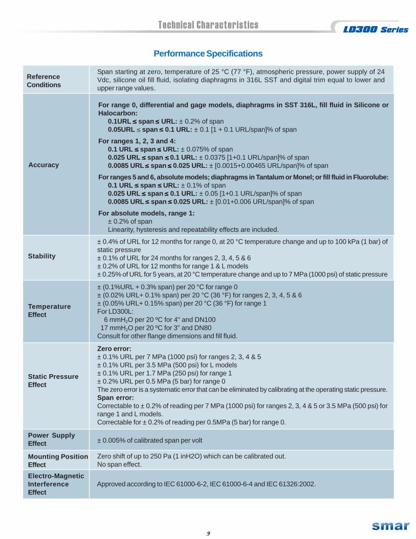
9
Performance Specifications
ReferenceConditions
Span starting at zero, temperature of 25 °C (77 °F), atmospheric pressure, power supply of 24Vdc, silicone oil fill fluid, isolating diaphragms in 316L SST and digital trim equal to lower andupper range values.
Zero error:± 0.1% URL per 7 MPa (1000 psi) for ranges 2, 3, 4 & 5± 0.1% URL per 3.5 MPa (500 psi) for L models± 0.1% URL per 1.7 MPa (250 psi) for range 1± 0.2% URL per 0.5 MPa (5 bar) for range 0The zero error is a systematic error that can be eliminated by calibrating at the operating static pressure.Span error:Correctable to ± 0.2% of reading per 7 MPa (1000 psi) for ranges 2, 3, 4 & 5 or 3.5 MPa (500 psi) forrange 1 and L models.Correctable for ± 0.2% of reading per 0.5MPa (5 bar) for range 0.
Power SupplyEffect ± 0.005% of calibrated span per volt
Static PressureEffect
TemperatureEffect
± (0.1%URL + 0.3% span) per 20 °C for range 0± (0.02% URL+ 0.1% span) per 20 °C (36 °F) for ranges 2, 3, 4, 5 & 6± (0.05% URL+ 0.15% span) per 20 °C (36 °F) for range 1For LD300L: 6 mmH2O per 20 ºC for 4" and DN100 17 mmH2O per 20 ºC for 3" and DN80Consult for other flange dimensions and fill fluid.
± 0.4% of URL for 12 months for range 0, at 20 °C temperature change and up to 100 kPa (1 bar) ofstatic pressure± 0.1% of URL for 24 months for ranges 2, 3, 4, 5 & 6± 0.2% of URL for 12 months for range 1 & L models± 0.25% of URL for 5 years, at 20 °C temperature change and up to 7 MPa (1000 psi) of static pressure
Stability
Zero shift of up to 250 Pa (1 inH2O) which can be calibrated out.No span effect.
Mounting PositionEffect
Electro-MagneticInterferenceEffect
Approved according to IEC 61000-6-2, IEC 61000-6-4 and IEC 61326:2002.
Technical Characteristics
For range 0, differential and gage models, diaphragms in SST 316L, fill fluid in Silicone orHalocarbon:
0.1URL span URL: ± 0.2% of span0.05URL span 0.1 URL: ± 0.1 [1 + 0.1 URL/span]% of span
For ranges 1, 2, 3 and 4:0.1 URL span URL: ± 0.075% of span0.025 URL span 0.1 URL: ± 0.0375 [1+0.1 URL/span]% of span0.0085 URL span 0.025 URL: ± [0.0015+0.00465 URL/span]% of span
For ranges 5 and 6, absolute models; diaphragms in Tantalum or Monel; or fill fluid in Fluorolube:0.1 URL span URL: ± 0.1% of span0.025 URL span 0.1 URL: ± 0.05 [1+0.1 URL/span]% of span0.0085 URL span 0.025 URL: ± [0.01+0.006 URL/span]% of span
For absolute models, range 1:± 0.2% of spanLinearity, hysteresis and repeatability effects are included.
≤≤≤≤≤≤ ≤≤≤≤≤
≤≤≤≤≤
Accuracy≤≤≤≤≤ ≤≤≤≤≤
≤≤≤≤≤
≤≤≤≤≤
≤≤≤≤≤ ≤≤≤≤≤≤≤≤≤≤ ≤≤≤≤≤≤≤≤≤≤ ≤≤≤≤≤
≤≤≤≤≤
≤≤≤≤≤
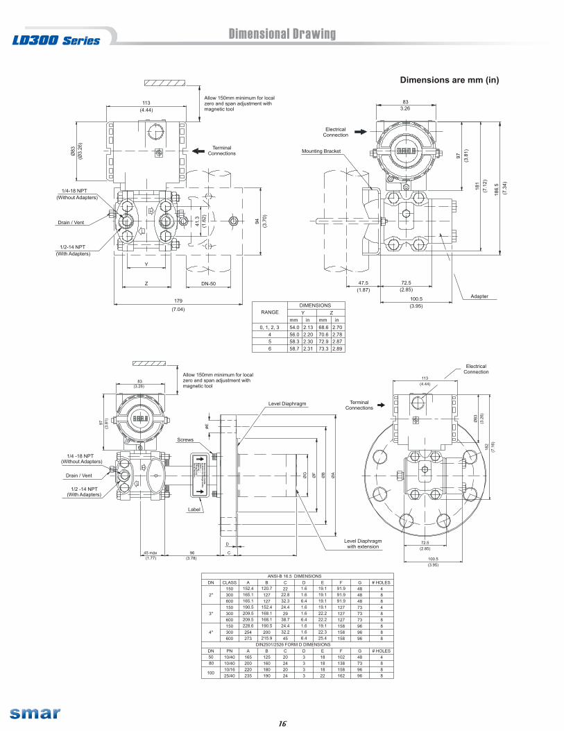
16
Dimensional Drawing

5 VDC OUTPUT IS® PRESSURE TRANSDUCER
OPTIONAL CONNECTOR VERSIONHERMETICALLY SEALED
ETM-375 (M) SERIES ETL-375 (M) SERIES• 5 VDC Output• Hybrid Microelectronic Regulator-Amplifier• Flush Diaphragm• All Welded Construction• Secondary Containment OnAbsolute And Sealed Units• Flight Qualified• 3/8-24 UNJF or M10 X 1 Thread• 4 Wire (ETM-375) 3 Wire (ETM-300-375)
these transducers without the screen. The ETL Series uses Kulite's PatentedLeadless Technology.
Incorporation of a Kulite proprietary electronics module within the main body ofthis product allows for operation from an unregulated power supply ranging from13 to 32 VDC. Standard output is a stable, low noise 0 to 5 VDC signal.
ETM-375 series transducers are miniature, threaded flush diaphragm instruments. Theyutilize a flush metal diaphragm as a force collector. Force is transferred to a solid statepiezoresistive sensing element via a thin intervening film of non-compressible siliconeoil. This sensing sub-assembly is protected from mechanical damage by a solid screenwhich has been shown to have minimal influence of the frequency response of thesensor. For applications where a true flush diaphragm is needed, Kulite will supply
PTIH-8-4PCONNECTOR
.50 MAX.
5/8 HEX(15.9)
.32 (8.1)NOM.
.625 DIA.(15.9)
4 COND. # 30 AWGSHIELDED CABLE30" (762) LONG
.56 DIA.(14.2)
HEX PROFILEAFTER CRIMPING
CABLE STRAIN RELIEF
"M" SCREEN
3/8–24 UNJF–3A(M 10 X 1)
O – RING.301 I.D. X .064 C.S.(7.6 I.D. X 1.6 C.S.)
LOCKWIRE HOLES.040 DIA. (1.0) (2) PLC'S
.42(10.8)
.16 (4.1) NOM.
.32(8.1)
.81 (20.6) NOM..17(4.3)
KULITE SEMICONDUCTOR PRODUCTS, INC. • One Willow Tree Road • Leonia, New Jersey 07605 • Tel: 201 461-0900 • Fax: 201 461-0990 • http://www.kulite.com
Note: Custom pressure ranges, accuracies and mechanical configurations available.Continuous development and refinement of our products may result in specification changes without notice - all dimensions nominal.
123
TUPNIegnaRerusserP
7.152
5.305
7001
71052
53005
070001
0710052
0530005
00700001
RAB0041ISP00002
edoMlanoitarepO egaGdelaeS,egaG,etulosbA
erusserPrevO5.305
7001
41002
53005
25057
5010051
0120003
5250057
050100051
RAB0012ISP00003
erusserPtsruB )RAB0042(ISP00053fo.xaMaoterusserPdetaRsemiT3
aideMerusserP gniR-OdetceleSdnaSS613roHP4-71htiWelbitapmoCsaGrodiuqiLynA
noitaticxElacirtcelEdetaR )redrOlaicepSnoelbaliavAstupnIrehtO(CDV23-31
tnerruClacirtcelEmumixaM am52
TUPTUOecnadepmItuptuO
).pyT(smhO002
)OSF(tuptuOelacSlluF %3±V5
)Bd3–(htdiwdnaB zHK5otCD
ecnalabnUlaudiseR )573-MTE(Vm001ot0 )573-003-MTE(Vm05±Vm002
siseretsyH,ytiraeniL-noNdenibmoCytilibataepeRdna LSFB).xaMSF%52.0±().pyT(LSFBSF%1.0±
siseretsyH ).pyT(OSF%1.0±
ytilibataepeR ).pyT(OSF%1.0±
noituloseR lamisetinifnI
).pyT()zHK(ycneuqerFlarutaN 021 012 582 524 055 027 019 0211 0531 0061
g/SF%ytivitisneSnoitareleccAralucidnepreP
esrevsnarT01x9.1 3-
01x9.1 5-01x0.1 3-
01x0.1 5-01x2.5 4-
01x2.5 7-01x2.2 4-
01x2.2 7-01x1.1 4-
01x1.1 7-01x2.6 5-
01x2.6 8-01x6.2 5-
01x6.2 8-01x5.1 5-
01x5.1 8-01x6.8 6-
01x6.8 9-01x2.5 6-
01x2.5 9-
ecnatsiseRnoitalusnI CDV05ta.niMmhogeM001
LATNEMNORIVNEegnaRerutarepmeTgnitarepO
)C°021+otC°55–(F°052+otF°56–
egnaRerutarepmeTdetasnepmoC tseuqeRnodetouQsegnaRrehtO)C°001+otC°81–(F°212+otF°0
tfihSoreZlamrehT ).pyT()C°55(F°001/OSF%1±
tfihSytivitisneSlamrehT ).pyT()C°55(F°001/OSF%1±
noitarbiVraeniL zH0005otpueniS,kaePg001
edutitlA detceffanU
ytidimuH ytidimuHevitaleR%001
kcohSlacinahceM .cesµ001g0005,.cesm11g001
LACISYHPnoitcennoClacirtcelE
gnoL)267("03elbaCdedleihSGWA03rotcudnoC4
thgieW elbaCgnidulcxE).xaM(smarG5.42
elpicnirPgnisneS nociliSnonociliSdetalosIyllacirtceleiDegdirBenotstaehWmrAruoFevitcAylluF
euqroTgnitnuoM ).xaM(sdnuoP-hcnI08
NIP NOITANGISEDA TUPNI+B TUPNI–C TUPTUO+D TUPTUO–
ROLOC NOITANGISEDDER TUPNI+
KCALB TUPNI–NEERG + TUO TUPETIHW TUPTUO–
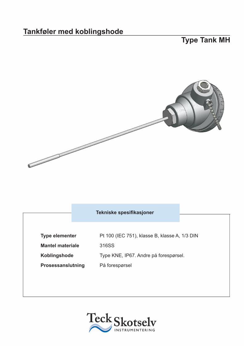
Tankføler med koblingshode
Tekniske spesifi kasjoner
Type elementer Pt 100 (IEC 751), klasse B, klasse A, 1/3 DIN Mantel materiale 316SS Koblingshode Type KNE, IP67. Andre på forespørsel. Prosessanslutning På forespørsel
Type Tank MH
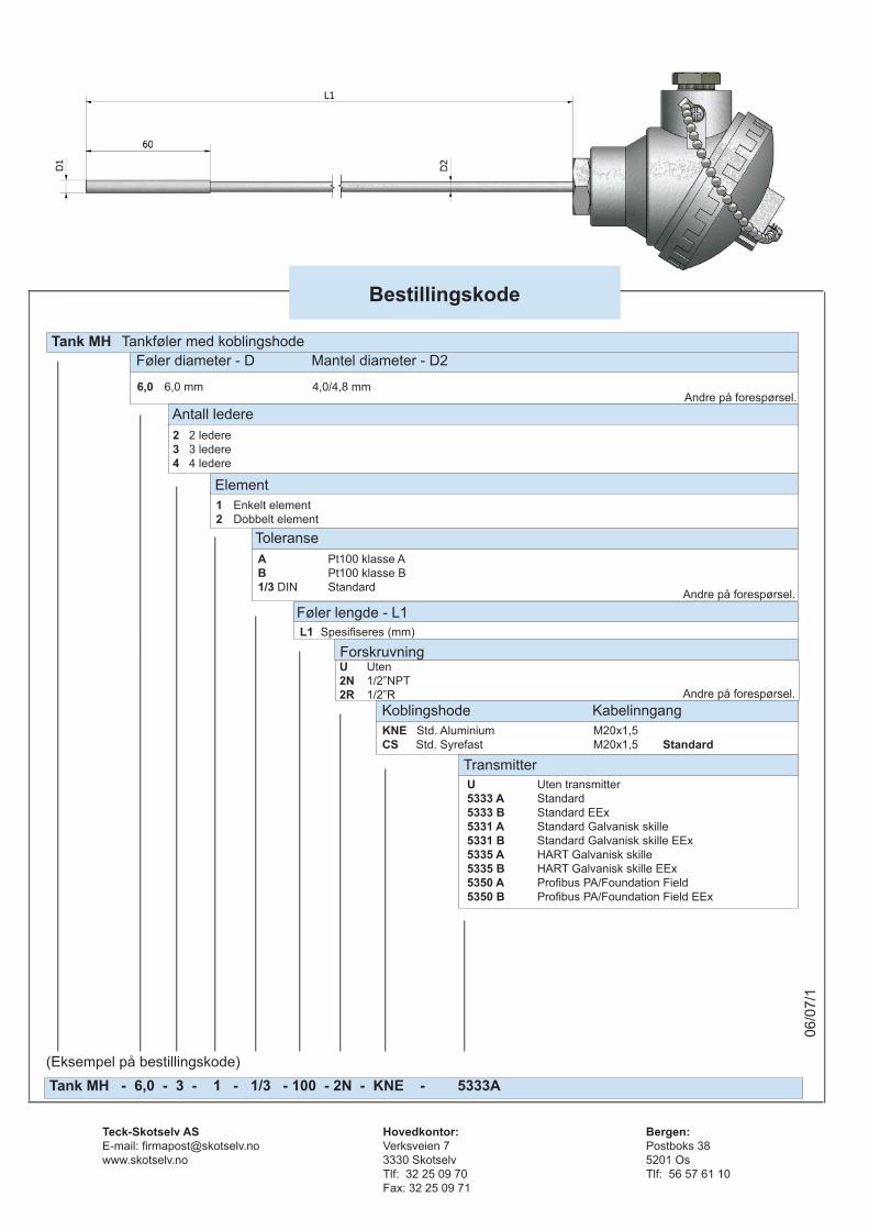
U Uten transmitter5333 A Standard5333 B Standard EEx5331 A Standard Galvanisk skille5331 B Standard Galvanisk skille EEx5335 A HART Galvanisk skille5335 B HART Galvanisk skille EEx5350 A Profi bus PA/Foundation Field5350 B Profi bus PA/Foundation Field EEx
Bestillingskode
1 Enkelt element2 Dobbelt element
L1 Spesifi seres (mm)
Føler diameter - D Mantel diameter - D2
6,0 6,0 mm 4,0/4,8 mm
Antall ledere
Element
ToleranseA Pt100 klasse AB Pt100 klasse B1/3 DIN Standard
Føler lengde - L1
Forskruvning
Tank MH Tankføler med koblingshode
Tank MH - 6,0 - 3 - 1 - 1/3 - 100 - 2N - KNE - 5333A (Eksempel på bestillingskode)
06/0
7/1
U Uten2N 1/2”NPT2R 1/2”R
Andre på forespørsel.
Andre på forespørsel.
Koblingshode KabelinngangKNE Std. Aluminium M20x1,5 CS Std. Syrefast M20x1,5 Standard
Andre på forespørsel.
Transmitter
2 2 ledere3 3 ledere4 4 ledere
Teck-Skotselv AS Hovedkontor: Bergen:E-mail: fi [email protected] Verksveien 7 Postboks 38www.skotselv.no 3330 Skotselv 5201 Os Tlf: 32 25 09 70 Tlf: 56 57 61 10 Fax: 32 25 09 71

AUTEK
0,0000
RF
SHEET: 1 OF 1
SPEC#: REV: 01
JOB # :
P.O. :
DATE : 14.04.2008 CHK:
BY : LKS APR:
Data sheet for
FLOW ELEMENTNO BY DATE
150#
304 SS
NTNU
FEOR-010
Calculation
NTNU
ELEMENT DATA
:
::
FE-003-Tilbud ::
:
: Orifice Plate-Standard: /::
304 SS0,4018
: 100,4458 mm: mm
SIZING CRITERIA : Exact Differential: ISO 5167-2003
PIPING DATA :::::
250,0000 mm
316 SS
/
COEFFICIENTS : 0,603 : 1,000: 0,988 :
: 140508,82 : 1,013: 349712,89 : 736110
PROCESS DATA Base Maximum Flow Normal Flow Property Method
: 0,50 kg/sec: 45,98 millibar::
37,761,00
millibarBar
:: 20,00 DEG C: 1,19 kg/m3 Redlich-Kwong:::
0,9990,02 cP User Input
: 1,4016 Redlich-Kwong Equation: Air / Gas::
UNCERTAINTY DATA :: ±0,50%: ±0,11%: ±0,05%::
±0,30%
:
Notes :
This report created by Flowel 4.0
Press. Tap Loc. / TypeElement Type
Element MaterialBeta Ratio(d/D)Element BoreThickness
Sizing ModeReference
FlangePipe Size & SCHPipe I.D.Flange MaterialPipe Material
Discharge Coeff.(C)Gas Expan. Coeff.(Y1)Reynolds No.(Pipe)Reynolds No.(Bore)
Flow RateDiff. PressurePressure LossStatic PressureBase PressureTemperatureDensitySpec. GravityZ-Compressibility FactorViscosityk-Factor (Cp/Cv)Fluid Name / Fluid StateLiquid DensityGas Quality
Uncertainty in Flow Ratein Discharge Coeff.in Expansion Factorin Primary Diameterin Pipe Diameterin Densityin Pressure
Velocity of Approach Factor (Ev)Reynolds No.(Pipe - Normal)
Murdock Wet Gas Factor (Fx)User Factor (Fuser)
Tag. No.Service
Manuf.
Eq./Line No.Flowsheet
Model No.
PRINTED:22.08.2008 08:42:51
Upstream Corner

KIMO offers a wide range of high-quality and accurate Pitot tubes, as per the AFNOR NFX 10-112 norm.These Pitot tubes, when being connected to a differential column / or needle / or electronical manometer, can measure the dynamic
3pressure of a moving fluid in a duct, and then can deduct its air velocity in m/s and its airflow in m /h.These Pitot tubes are used in HVAC field, vacuum cleaning and pneumatical transport. They are mainly dedicated to measure hot and particle-charged air, and also high air velocity.
Pitot tube with ellipsoidal head.An intake for total pressure and 6 holes for static pressure.Body made of stainless steel.
Pitot tubes Type L
Norm
Model
Coefficient
Accuracy
Quality
Operatingtemperature
AFNOR NFX10-112. Annex 4 dated 14.9.77.This norm meets the requirements of the International Norm ISO 3966.
NPL curved with ellipsoidal head
1,0015
More than 1 %, for a ± 10 ° alignment to the fluid flow.
Hard stainless steel 4/4, as per AFNOR / Z2.CDN.17.12.
From 0 to 600 °C in standard and up to 1000 °C in option (except Ø 3 mm).
Pitot tube with ellipsoidal head.An intake for total pressure and 6 holes for static pressure.Sheated thermocouple K probe integrated, with connection cable length 1,5 m.Body made of stainless steel.
Pitot tubes Type L with TC K
Type L Type L with TC K
The extent error of an air velocity or airflow measurement with a KIMO Pitot tube remains inferior to 2%, when being carried out as per the NFX10-112 norm.
It is recommended to carry out a calibration of the Pitot tube, in order to determine its exact coefficient.
Integrated Temperature probe
PITOT TUBEStype L
CONSTRUCTEUR
TECHNICAL DATA SHEET
Air velocity Pressure Humidity Air flow Temperature
weN weN weN
weN
!!
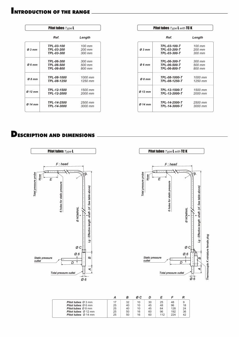
Ref. Length
TPL-03-100 100 mmTPL-03-200 200 mmTPL-03-300 300 mm
TPL-06-300 300 mmTPL-06-500 500 mmTPL-06-800 800 mm
TPL-08-1000 1000 mmTPL-08-1250 1250 mm
TPL-12-1500 1500 mmTPL-12-2000 2000 mm
TPL-14-2500 2500 mmTPL-14-3000 3000 mm
F : headF : head
RR
6 h
ole
s fo
r st
atic
pre
ssu
re6
ho
les
for
sta
tic p
ress
ure
Lg
: E
ffe
ctiv
e le
ng
th -
sha
ft-
(cf. S
ee
ta
ble
ab
ove
)L
g : E
ffe
ctiv
e le
ng
th -
sha
ft-
(cf. S
ee
ta
ble
ab
ove
)
Ø N
OM
INA
LØ
NO
MIN
AL
BB
Ø CØ C
Ø 6Ø 6
DD
AA
Ø 6Ø 6
Total pressure outletTotal pressure outlet
F : headF : head
EENo
seN
ose
RR
6 h
ole
s fo
r st
atic
pre
ssu
re6
ho
les
for
sta
tic p
ress
ure
Ø N
OM
INA
LØ
NO
MIN
AL
BB
Ø CØ C
Ø 6Ø 6
DD
AA
Th
erm
oco
up
le K
min
iatu
re fe
ma
le p
lug
Th
erm
oco
up
le K
min
iatu
re fe
ma
le p
lug
Ø 6Ø 6
A B Ø C D E F R
Ø 3 mm
Ø 6 mm
Ø 8 mm
Ø 12 mm
Ø 14 mm
Pitot tubes Ø 3 mm 17 32 10 30 25 48 9Pitot tubes Ø 6 mm 25 40 10 45 48 96 18Pitot tubes Ø 8 mm 25 40 10 45 64 128 24Pitot tubes Ø 12 mm 25 50 16 60 96 192 36Pitot tubes Ø 14 mm 25 50 16 60 112 224 42
To
tal p
ress
ure
pro
be
To
tal p
ress
ure
pro
be
Static pressureoutletStatic pressureoutlet
EENo
seN
ose
To
tal p
ress
ure
pro
be
To
tal p
ress
ure
pro
be
Pitot tubes Type L Pitot tubes Type L with TC K
Pitot tubes Type L Pitot tubes Type L with TC K
Ref. Length
TPL-03-100-T 100 mmTPL-03-200-T 200 mmTPL-03-300-T 300 mm
TPL-06-300-T 300 mmTPL-06-500-T 500 mmTPL-06-800-T 800 mm
TPL-08-1000-T 1000 mmTPL-08-1250-T 1250 mm
TPL-12-1500-T 1500 mmTPL-12-2000-T 2000 mm
TPL-14-2500-T 2500 mmTPL-14-3000-T 3000 mm
Ø 3 mm
Ø 6 mm
Ø 8 mm
Ø 12 mm
Ø 14 mm
Lg
: E
ffe
ctiv
e le
ng
th -
sha
ft-
(cf. S
ee
ta
ble
ab
ove
)L
g : E
ffe
ctiv
e le
ng
th -
sha
ft-
(cf. S
ee
ta
ble
ab
ove
)
Static pressureoutletStatic pressureoutlet
Total pressure outletTotal pressure outlet
INTRODUCTION OF THE RANGE
DESCRIPTION AND DIMENSIONS
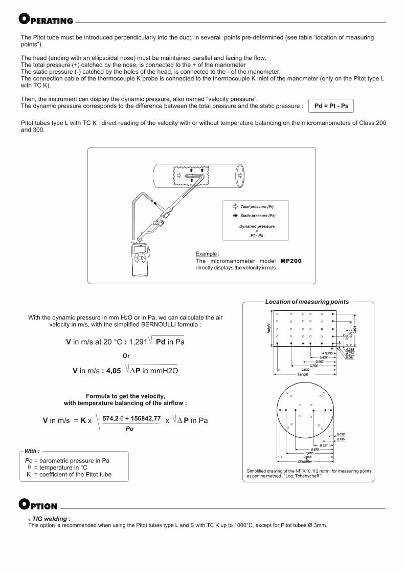
He
igh
tH
eig
ht
0,0610,061
0,0740,074
LengthLength
0,9390,939
0,7650,765
0,5630,563
0,4370,437
0,2350,2350
,92
60
,92
6
0,7
12
0,7
12
0,5
0,5
0,2880,288
0,1350,135
0,0320,032
0,9680,9680,8650,865
0,6790,679
0,3210,321
DiameterDiameter
The Pitot tube must be introduced perpendicularly into the duct, in several points pre-determined (see table “location of measuring points”).
The head (ending with an ellipsoidal nose) must be maintained parallel and facing the flow. The total pressure (+) catched by the nose, is connected to the + of the manometerThe static pressure (-) catched by the holes of the head, is connected to the - of the manometer.The connection cable of the thermocouple K probe is connected to the thermocouple K inlet of the manometer (only on the Pitot type L with TC K).
Then, the instrument can display the dynamic pressure, also named “velocity pressure”.The dynamic pressure corresponds to the difference between the total pressure and the static pressure : Pd = Pt - Ps
Location of measuring points
Pitot tubes type L with TC K : direct reading of the velocity with or without temperature balancing on the micromanometers of Class 200 and 300.
- +
Example :
The micromanometer model MP200 directly displays the velocity in m/s.
With the dynamic pressure in mm H2O or in Pa, we can calculate the air velocity in m/s, with the simplified BERNOULLI formula :
V in m/s at 20 °C : 1,291 Pd in Pa
Or
V in m/s : 4,05 P in mmH2O
Formula to get the velocity, with temperature balancing of the airflow :
V in m/s = K x x P in PaPo
Simplified drawing of the NF.X10.112 norm, for measuring points, as per the method “Log. Tchebycheff ”.
! TIG welding : This option is recommended when using the Pitot tubes type L and S with TC K up to 1000°C, except for Pitot tubes Ø 3mm.
Po = barometric pressure in Pa = temperature in °C K = coefficient of the Pitot tube
With :
Total pressure (Pt)
Static pressure (Ps)
Dynamic pressure=
Pt - Ps
E
OPERATING
OPTION
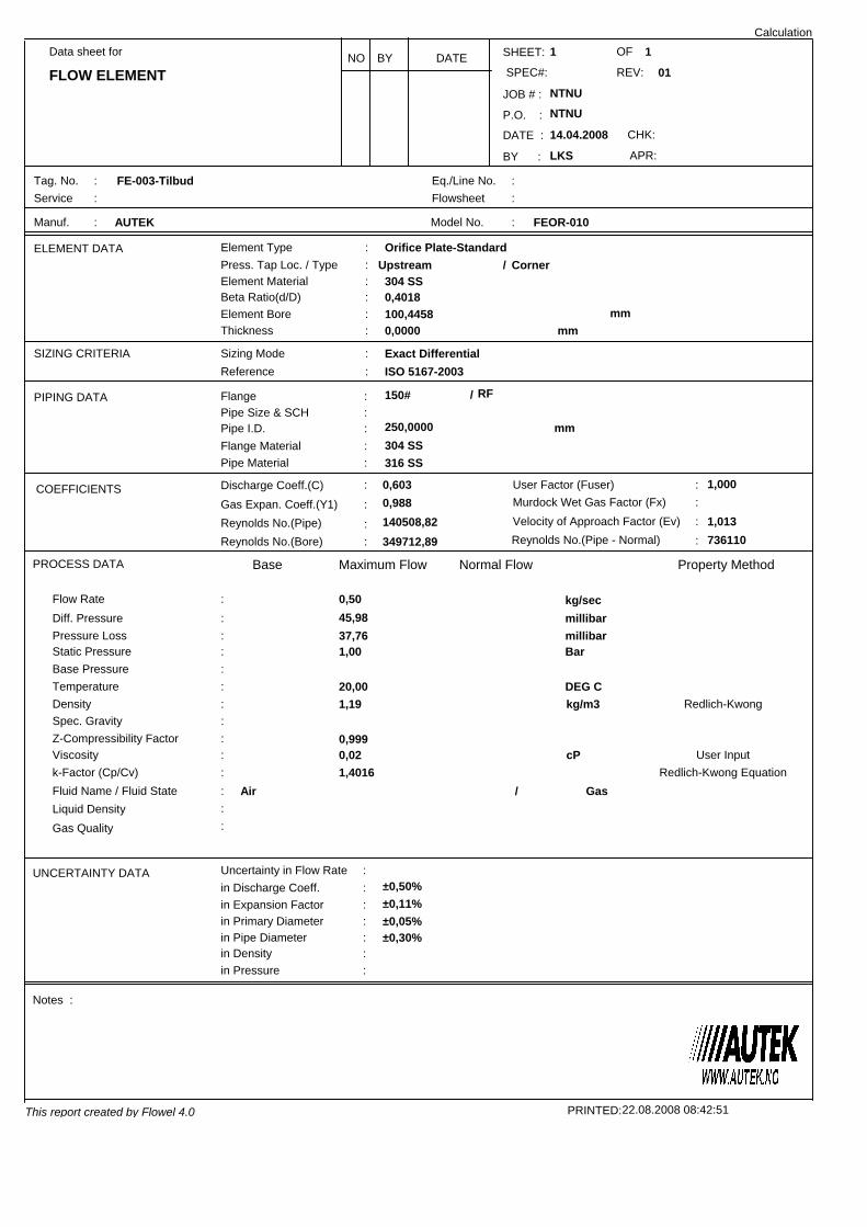
AUTEK
0,0000
RF
SHEET: 1 OF 1
SPEC#: REV: 01
JOB # :
P.O. :
DATE : 14.04.2008 CHK:
BY : LKS APR:
Data sheet for
FLOW ELEMENTNO BY DATE
150#
304 SS
NTNU
FEOR-010
Calculation
NTNU
ELEMENT DATA
:
::
FE-003-Tilbud ::
:
: Orifice Plate-Standard: /::
304 SS0,4018
: 100,4458 mm: mm
SIZING CRITERIA : Exact Differential: ISO 5167-2003
PIPING DATA :::::
250,0000 mm
316 SS
/
COEFFICIENTS : 0,603 : 1,000: 0,988 :
: 140508,82 : 1,013: 349712,89 : 736110
PROCESS DATA Base Maximum Flow Normal Flow Property Method
: 0,50 kg/sec: 45,98 millibar::
37,761,00
millibarBar
:: 20,00 DEG C: 1,19 kg/m3 Redlich-Kwong:::
0,9990,02 cP User Input
: 1,4016 Redlich-Kwong Equation: Air / Gas::
UNCERTAINTY DATA :: ±0,50%: ±0,11%: ±0,05%::
±0,30%
:
Notes :
This report created by Flowel 4.0
Press. Tap Loc. / TypeElement Type
Element MaterialBeta Ratio(d/D)Element BoreThickness
Sizing ModeReference
FlangePipe Size & SCHPipe I.D.Flange MaterialPipe Material
Discharge Coeff.(C)Gas Expan. Coeff.(Y1)Reynolds No.(Pipe)Reynolds No.(Bore)
Flow RateDiff. PressurePressure LossStatic PressureBase PressureTemperatureDensitySpec. GravityZ-Compressibility FactorViscosityk-Factor (Cp/Cv)Fluid Name / Fluid StateLiquid DensityGas Quality
Uncertainty in Flow Ratein Discharge Coeff.in Expansion Factorin Primary Diameterin Pipe Diameterin Densityin Pressure
Velocity of Approach Factor (Ev)Reynolds No.(Pipe - Normal)
Murdock Wet Gas Factor (Fx)User Factor (Fuser)
Tag. No.Service
Manuf.
Eq./Line No.Flowsheet
Model No.
PRINTED:22.08.2008 08:42:51
Upstream Corner

Appendix D: Risk assessment report
Appendix D: Risk assessment report
Risk Assessment Report
[Wet gas impeller test facility]
Prosjekttittel Prosjektleder Lars Erik Bakken Enhet NTNU HMS-koordinator Erik Langørgen Linjeleder Olav Bolland Plassering Romnummer Riggansvarlig [Trond Grüner] Risikovurdering utført av
Lars Andreas Øvrum Sørvik, Erik Mele, Dag Remi Reitan.
TABLE OF CONTENTS
1 INTRODUCTION ................................................................................................................ I
2 ORGANISATION ................................................................................................................ I
3 RISK MANAGEMENT IN THE PROJECT ............................................................................. II
4 DRAWINGS, PHOTOS, DESCRIPTIONS OF TEST SETUP .................................................... II
5 EVACUATION FROM THE EXPERIMENT AREA ................................................................ III
6 WARNING ....................................................................................................................... III
6.1 Before experiments ........................................................................................................ iii 6.2 Nonconformance ............................................................................................................ iii
7 VURDERING AV TEKNISK SIKKERHET .............................................................................. IV
7.1 Fareidentifikasjon, HAZOP.............................................................................................. iv 7.2 Flammable, reactive and pressurized substances and gas ............................................ iv 7.3 Pressurized equipment ................................................................................................... iv 7.4 Effects to environment (emissions to air water, noise, temperature, vibration, smell) v 7.5 Radiation ......................................................................................................................... v 7.6 Usage and handling of chemicals. ................................................................................... v 7.7 El safety (need to deviate from the current regulations and standards.) ...................... v
8 ASSESSMENT OF OPERATIONAL SAFETY ......................................................................... V
8.1 Prosedure HAZOP ............................................................................................................ v 8.2 Operation and emergency shutdown procedure............................................................ v 8.3 Training of operators ....................................................................................................... v 8.4 Technical modifications .................................................................................................. vi 8.5 Personal protective equipment ...................................................................................... vi
8.5.1 Generelt ............................................................. Error! Bookmark not defined. 8.6 Safety equipment ........................................................................................................... vi 8.7 Special actions. ............................................................................................................... vi
9 QUANTIFYING OF RISK - RISK MATRIX............................................................................ VI
10 CONCLUSJON ................................................................................................................. VII
11 LOVER FORSKRIFTER OG PÅLEGG SOM GJELDER .... ERROR! BOOKMARK NOT DEFINED.
12 DOCUMENTATION ........................................................................................................... X
13 VEILEDNING TIL RAPPORTMAL ................................ ERROR! BOOKMARK NOT DEFINED.
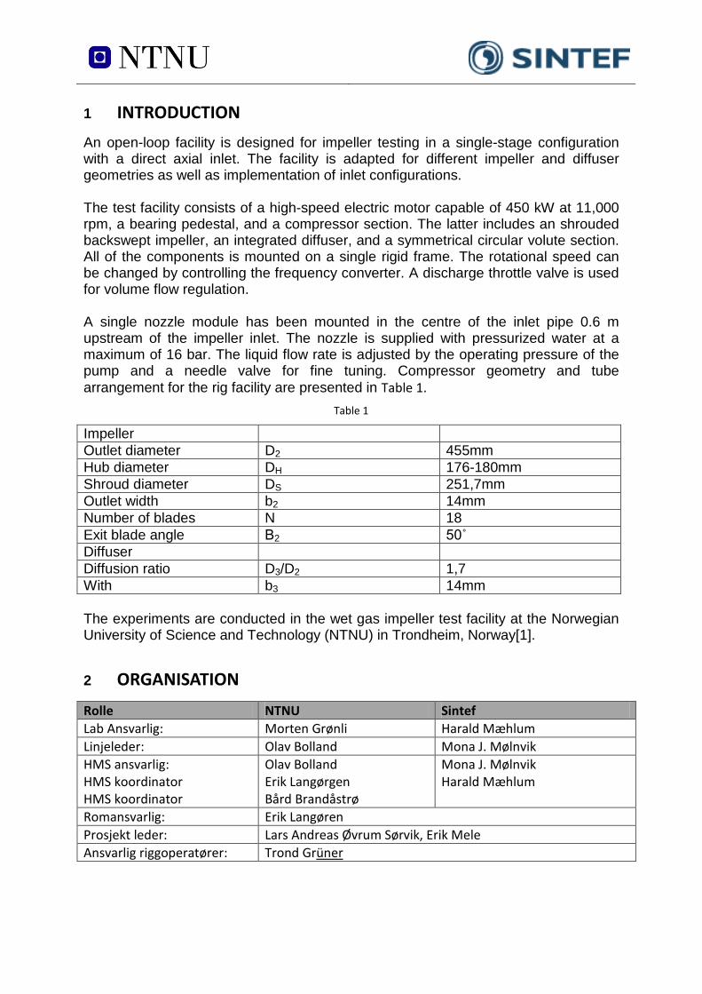
1 INTRODUCTION An open-loop facility is designed for impeller testing in a single-stage configuration with a direct axial inlet. The facility is adapted for different impeller and diffuser geometries as well as implementation of inlet configurations. The test facility consists of a high-speed electric motor capable of 450 kW at 11,000 rpm, a bearing pedestal, and a compressor section. The latter includes an shrouded backswept impeller, an integrated diffuser, and a symmetrical circular volute section. All of the components is mounted on a single rigid frame. The rotational speed can be changed by controlling the frequency converter. A discharge throttle valve is used for volume flow regulation. A single nozzle module has been mounted in the centre of the inlet pipe 0.6 m upstream of the impeller inlet. The nozzle is supplied with pressurized water at a maximum of 16 bar. The liquid flow rate is adjusted by the operating pressure of the pump and a needle valve for fine tuning. Compressor geometry and tube arrangement for the rig facility are presented in Table 1.
Table 1
Impeller Outlet diameter D2 455mm Hub diameter DH 176-180mm Shroud diameter DS 251,7mm Outlet width b2 14mm Number of blades N 18 Exit blade angle Β2 50˚ Diffuser Diffusion ratio D3/D2 1,7 With b3 14mm The experiments are conducted in the wet gas impeller test facility at the Norwegian University of Science and Technology (NTNU) in Trondheim, Norway[1].
2 ORGANISATION
Rolle NTNU Sintef Lab Ansvarlig: Morten Grønli Harald Mæhlum Linjeleder: Olav Bolland Mona J. Mølnvik HMS ansvarlig: HMS koordinator HMS koordinator
Olav Bolland Erik Langørgen Bård Brandåstrø
Mona J. Mølnvik Harald Mæhlum
Romansvarlig: Erik Langøren Prosjekt leder: Lars Andreas Øvrum Sørvik, Erik Mele Ansvarlig riggoperatører: Trond Grüner
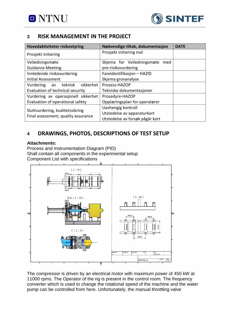
3 RISK MANAGEMENT IN THE PROJECT
Hovedaktiviteter risikostyring Nødvendige tiltak, dokumentasjon DATE
Prosjekt initiering Prosjekt initiering mal
Veiledningsmøte Guidance Meeting
Skjema for Veiledningsmøte med pre-risikovurdering
Innledende risikovurdering Initial Assessment
Fareidentifikasjon – HAZID Skjema grovanalyse
Vurdering av teknisk sikkerhet Evaluation of technical security
Prosess-HAZOP Tekniske dokumentasjoner
Vurdering av operasjonell sikkerhet Evaluation of operational safety
Prosedyre-HAZOP Opplæringsplan for operatører
Sluttvurdering, kvalitetssikring Final assessment, quality assurance
Uavhengig kontroll Utstedelse av apparaturkort Utstedelse av forsøk pågår kort
4 DRAWINGS, PHOTOS, DESCRIPTIONS OF TEST SETUP Attachments: Process and Instrumentation Diagram (PID) Shall contain all components in the experimental setup Component List with specifications
The compressor is driven by an electrical motor with maximum power of 450 kW at 11000 rpms. The Operator of the rig is present in the control room. The frequency converter which is used to change the rotational speed of the machine and the water pump can be controlled from here. Unfortunately, the manual throttling valve

downstream the compressor cannot be closed from the control room. Therefore, in order for attain transient conditions, the regulation of volume flow is done manually. To ensure that the injection of water provides an equal distribution, 16 nozzles is distributed uniformly over the circumference of the tube. The water pump is capable of flows up to 50kg/s at 16bar.
5 EVACUATION FROM THE EXPERIMENT AREA Evacuate at signal from the alarm system or local gas alarms with its own local alert with sound and light outside the room in question, see 6.2 Evacuation from the rigging area takes place through the marked emergency exits to the meetingpoint, (corner of Old Chemistry Kjelhuset or parking 1a-b.) Action on rig before evacuation: (Shut off the air and water supply. Power off the electrical supply.)
6 WARNING
6.1 Before experiments
E-mail with information about the test run duration, (hour) and the involved to HMS koordinator NTNU/SINTEF
[email protected] [email protected]
Project Managers on neighboring units alerted for clarification around the use of the exhaust system without fear or interference of any kind, see rig matrix. All experiments should be planned and put into the activity calendar for the lab. Experiment leader must get confirmation that the experiments are coordinated with other activity before start up.
6.2 Nonconformance
FIRE Fire you are not able to put out with locally available fire extinguishers, activate, the nearest fire alarm and evacuate area. Be then available for fire brigade and building caretaker to detect fire place. If possible, notifie: NTNU SINTEF Labsjef Morten Grønli, tlf: 918 97 515 Labsjef Harald Mæhlum tlf 930 149 86 HMS: Erik Langørgen, tlf: 91897160 Forskningssjef Mona J Mølnvik tlf 930 08 868 Instituttleder: Olav Bolland: 91897209 GASALARM At a gas alarm, close gas bottles immediately and ventilated the area. If the level of gas concentration not decrease within a reasonable time, activate the fire alarm and

evacuate the lab. Designated personnel or fire department checks the leak to determine whether it is possible to seal the leak and ventilate the area in a responsible manner. Alert Order in the above paragraph. PERSONAL INJURY • First aid kit in the fire / first aid stations • Shout for help • Start life-saving first aid• CALL 113 if there is any doubt whether there is a serious injury Other Nonconformance (AVVIK) NTNU: Reporting form for nonconformance at: http://www.ntnu.no/hms/2007_Nettsider/HMSRV0401_avvik.doc SINTEF: Synergi
7 ASSESSMENT OF TECHNICAL SAFETY
7.1 HAZOP
See Chapter 14 "Guide to the report template”. Explosive zones Zone 0 Always explosive area, for instance vessels with pressurized gas, or flamable liquid Zone 1 Occasionally explosive zone, for instance fuel stations Zone 2 Secondary emission discharge site, may be explosive due to accidents Attachments:, skjema: Hazop_mal Conclusion: The testrig is not classified as any of the descriptions above, it is not necessary to take EX precautions
7.2 Flammable, reactive and pressurized substances and gas
Contains the experiments Flammable, reactive and pressurized substances and gas
Attachments: Hazop template
7.3 Pressurized equipment
Contain the set up pressurized equipment? Yes Equipment have to undergo pressure testes in accordance with the norms and be
documented Attachements:
No

7.4 Effects on the environment (emissions, noise, temperature, vibration, smell)
Yes Conclusion: The experimens will generate large amounts of noise and vibrations. Therefore, experiments at high speeds are scheduled after normal work hours. An eventual oil leakage will be minor and will be handled locally.
7.5 Radiation
See Chapter 14 "Guide to the report template”. No
7.6 Usage and handling of chemicals.
See Chapter 14 "Guide to the report template”. No
7.7 El safety (need to deviate from the current regulations and standards.)
Yes Stay clear of perimeter during operational hours
8 ASSESSMENT OF OPERATIONAL SAFETY
Ensures that established procedures cover all identified risk factors that must be taken care of through procedures. Ensures that the operators and technical performance have sufficient expertise.
8.1 Prosedure HAZOP
See Chapter 14 "Guide to the report template”. The method is a procedure to identify causes and sources of danger to operational problems. Attachments:: HAZOP_MAL_Prosedyre Conclusion:
8.2 Operation and emergency shutdown procedure
See Chapter 14 "Guide to the report template”. The operating procedure is a checklist that must be filled out for each experiment. Emergency procedure should attempt to set the experiment set up in a harmless state by unforeseen events. Attachments: ”Procedure for running experiments Emergency shutdown procedure:
8.3 Training of operators
A Document showing training plan for operators
What are the requirements for the training of operators? • What it takes to be an independent operator • Job Description for operators Attachments:: Training program for operators

8.4 Technical modifications
• Technical modifications made by the Operator o (for example: Replacement of components, equal to equal)
• • Technical modifications that must be made by Technical staff: o (for example, modification of pressure equipment).
Conclusion:
8.5 Personal protective equipment
Mandatory use of eye protection in the rig zone Mandatory use of hearing protection.
Conclusion:.
8.5.1 General Safety • The area around the staging attempts shielded. • Gantry crane and truck driving should not take place close to the experiment. • Gas cylinders shall be placed in an approved carrier with shut-off valve within
easy reach. • Monitoring, can experiment run unattended, how should monitoring be?
Conclusion: Is Operator allowed to leave during the experiment?
8.6 Safety equipment
• Have portable gas detectors to be used during test execution? • Warning signs, see the Regulations on Safety signs and signaling in the workplace
8.7 Special actions.
For example: • Monitoring. • Safety preparedness. • Safe Job Analysis of modifications, (SJA) • Working at heights • Flammable / toxic gases or chemicals
9 QUANTIFYING OF RISK - RISK MATRIX See Chapter 14 "Guide to the report template”. The risk matrix will provide visualization and an overview of activity risks so that management and users get the most complete picture of risk factors. IDnr Aktivitet-hendelse Frekv-Sans Kons RV xx Rotating shaft, locked room 1 C1 C1 Much noise, people without protective gear enter
the rig site Barriers and running experiments outside working hours
1 B1 B1

Conclusion : Participants will make a comprehensive assessment to determine whether the remaining risks of the activity / process is acceptable. Barriers and driving outside working hours e.g.
10 CONCLUSJON The rig is built in good laboratory practice (GLP). What technical changes or changes in operating parameters will require new risk assessment? (Other media, pressure, mechanical intervention) Experiment unit card get a period of XX months Experiment in progress card get a period of XX months

11 REGULATIONS AND GUIDELINES Se http://www.arbeidstilsynet.no/regelverk/index.html • Lov om tilsyn med elektriske anlegg og elektrisk utstyr (1929) • Arbeidsmiljøloven • Forskrift om systematisk helse-, miljø- og sikkerhetsarbeid (HMS Internkontrollforskrift) • Forskrift om sikkerhet ved arbeid og drift av elektriske anlegg (FSE 2006) • Forskrift om elektriske forsyningsanlegg (FEF 2006) • Forskrift om utstyr og sikkerhetssystem til bruk i eksplosjonsfarlig område NEK 420 • Forskrift om håndtering av brannfarlig, reaksjonsfarlig og trykksatt stoff samt utstyr og
anlegg som benyttes ved håndteringen • Forskrift om Håndtering av eksplosjonsfarlig stoff • Forskrift om bruk av arbeidsutstyr. • Forskrift om Arbeidsplasser og arbeidslokaler • Forskrift om Bruk av personlig verneutstyr på arbeidsplassen • Forskrift om Helse og sikkerhet i eksplosjonsfarlige atmosfærer • Forskrift om Høytrykksspyling • Forskrift om Maskiner • Forskrift om Sikkerhetsskilting og signalgivning på arbeidsplassen • Forskrift om Stillaser, stiger og arbeid på tak m.m. • Forskrift om Sveising, termisk skjæring, termisk sprøyting, kullbuemeisling, lodding og
sliping (varmt arbeid) • Forskrift om Tekniske innretninger • Forskrift om Tungt og ensformig arbeid • Forskrift om Vern mot eksponering for kjemikalier på arbeidsplassen
(Kjemikalieforskriften) • Forskrift om Vern mot kunstig optisk stråling på arbeidsplassen • Forskrift om Vern mot mekaniske vibrasjoner • Forskrift om Vern mot støy på arbeidsplassen Veiledninger fra arbeidstilsynet se: http://www.arbeidstilsynet.no/regelverk/veiledninger.html


12 DOCUMENTATION
• Tegninger, foto, beskrivelser av forsøksoppsetningen • Hazop_mal • Sertifikat for trykkpåkjent utstyr • Håndtering avfall i NTNU • Sikker bruk av LASERE, retningslinje • HAZOP_MAL_Prosedyre • Forsøksprosedyre • Opplæringsplan for operatører • Skjema for sikker jobb analyse, (SJA) • Apparaturkortet • Forsøk pågår kort

13 GUIDANCE TO RISK ASSESSMENT TEMPLATE Kap 7 Assessment of technical safety. Ensure that the design of the experiment set up is optimized in terms of technical safety. Identifying risk factors related to the selected design, and possibly to initiate re-design to ensure that risk is eliminated as much as possible through technical security. This should describe what the experimental setup actually are able to manage and acceptance for emission. 7.1 HAZOP The experimental set up is divided into nodes (eg motor unit, pump unit, cooling unit.). By using guidewords to identify causes, consequences and safeguards, recommendations and conclusions are made according to if necessary safety is obtained. When actions are performed the HAZOP is completed. (e.g. "No flow", cause: the pipe is deformed, consequence: pump runs hot, precaution: measurement of flow with a link to the emergency or if the consequence is not critical used manual monitoring and are written into the operational procedure.) 7.2 Flammable, reactive and pressurized substances and gas. According to the Regulations for handling of flammable, reactive and pressurized substances and equipment and facilities used for this: Flammable material: Solid, liquid or gaseous substance, preparation, and substance with occurrence or combination of these conditions, by its flash point, contact with other substances, pressure, temperature or other chemical properties represent a danger of fire. Reactive substances: Solid, liquid, or gaseous substances, preparations and substances that occur in combinations of these conditions, which on contact with water, by its pressure, temperature or chemical conditions, represents a potentially dangerous reaction, explosion or release of hazardous gas, steam, dust or fog. Pressurized : Other solid, liquid or gaseous substance or mixes havinig fire or hazardous material response, when under pressure, and thus may represent a risk of uncontrolled emissions Further criteria for the classification of flammable, reactive and pressurized substances are set out in Annex 1 of the Guide to the Regulations "Flammable, reactive and pressurized substances" http://www.dsb.no/Global/Publikasjoner/2009/Veiledning/Generell%20veiledning.pdf http://www.dsb.no/Global/Publikasjoner/2010/Tema/Temaveiledning_bruk_av_farlig_stoff_Del_1.pdf Experiment setup area should be reviewed with respect to the assessment of Ex zone • Zone 0: Always explosive atmosphere, such as inside the tank with gas, flammable liquid. • Zone 1: Primary zone, sometimes explosive atmosphere such as a complete drain

point • Zone 2: secondary discharge could cause an explosive atmosphere by accident, such as flanges, valves and connection points 7.4 Effects on the environment With pollution means: bringing solids, liquid or gas to air, water or ground, noise and vibrations, influence of temperature that may cause damage or inconvenience effect to the environment. Regulations: http://www.lovdata.no/all/hl-19810313-006.html#6 NTNU guidance to handling of waste:http://www.ntnu.no/hms/retningslinjer/HMSR18B.pdf 7.5 Radiation Definition of radiation Ionizing radiation: Electromagnetic radiation (in radiation issues with wawelength <100 nm) or rapid atomic particles (e.g. alpha and beta particles) with the ability to stream ionized atoms or molecules. Non ionizing radiation: Electromagnetic radiation (wavelength >100 nm), og ultrasound1 with small or no capability to ionize. Radiation sources: All ionizing and powerful non-ionizing radiation sources. Ionizing radiation sources: Sources giving ionizing radiation e.g. all types of radiation sources, x-ray, and electron microscopes. Powerful non ionizing radiation sources: Sources giving powerful non ionizing radiation which can harm health and/or environment, e.g. class 3B and 4. MR2 systems, UVC3 sources, powerful IR sources4. 1Ultrasound is an acoustic radiation ("sound") over the audible frequency range (> 20 kHz). In radiation protection regulations are referred to ultrasound with electromagnetic non-ionizing radiation. 2MR (e.g. NMR) - nuclear magnetic resonance method that is used to "depict" inner structures of different materials. 3UVC is electromagnetic radiation in the wavelength range 100-280 nm. 4IR is electromagnetic radiation in the wavelength range 700 nm - 1 mm. For each laser there should be an information binder (HMSRV3404B) which shall include: • General information • Name of the instrument manager, deputy, and local radiation protection coordinator • Key data on the apparatus • Instrument-specific documentation • References to (or copies of) data sheets, radiation protection regulations, etc. • Assessments of risk factors • Instructions for users • Instructions for practical use, startup, operation, shutdown, safety precautions, logging, locking, or use of radiation sensor, etc. • Emergency procedures See NTNU for laser: http://www.ntnu.no/hms/retningslinjer/HMSR34B.pdf 7.6 Usage and handling of chemicals. In the meaning chemicals, a element that can pose a danger to employee safety and health See: http://www.lovdata.no/cgi-wift/ldles?doc=/sf/sf/sf-20010430-0443.html
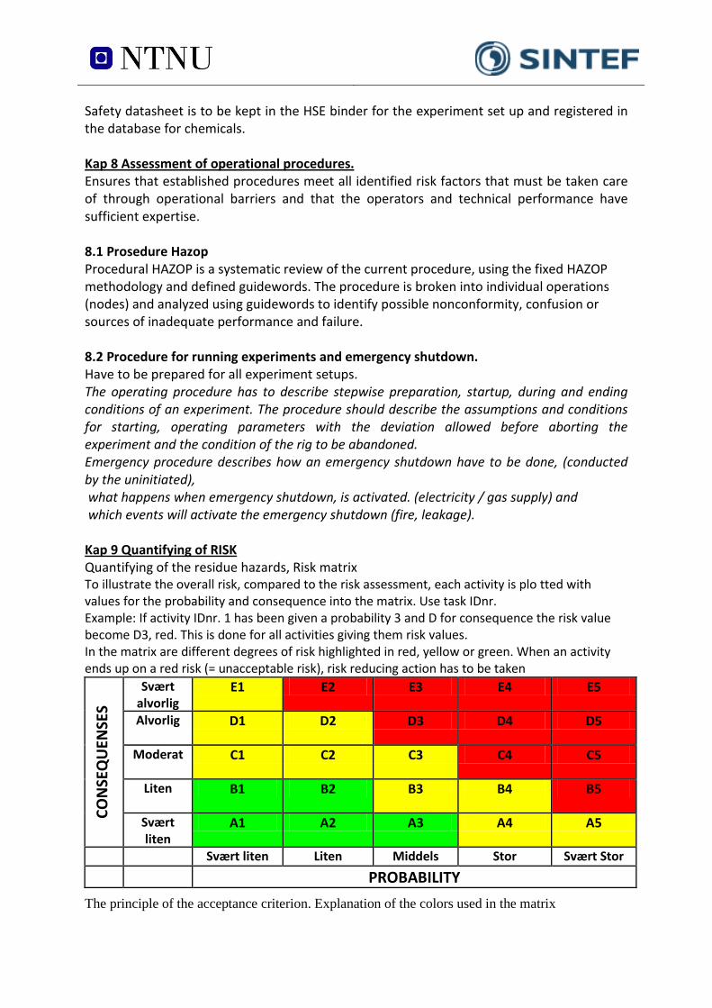
Safety datasheet is to be kept in the HSE binder for the experiment set up and registered in the database for chemicals. Kap 8 Assessment of operational procedures. Ensures that established procedures meet all identified risk factors that must be taken care of through operational barriers and that the operators and technical performance have sufficient expertise. 8.1 Prosedure Hazop Procedural HAZOP is a systematic review of the current procedure, using the fixed HAZOP methodology and defined guidewords. The procedure is broken into individual operations (nodes) and analyzed using guidewords to identify possible nonconformity, confusion or sources of inadequate performance and failure. 8.2 Procedure for running experiments and emergency shutdown. Have to be prepared for all experiment setups. The operating procedure has to describe stepwise preparation, startup, during and ending conditions of an experiment. The procedure should describe the assumptions and conditions for starting, operating parameters with the deviation allowed before aborting the experiment and the condition of the rig to be abandoned. Emergency procedure describes how an emergency shutdown have to be done, (conducted by the uninitiated), what happens when emergency shutdown, is activated. (electricity / gas supply) and which events will activate the emergency shutdown (fire, leakage). Kap 9 Quantifying of RISK Quantifying of the residue hazards, Risk matrix To illustrate the overall risk, compared to the risk assessment, each activity is plo tted with values for the probability and consequence into the matrix. Use task IDnr. Example: If activity IDnr. 1 has been given a probability 3 and D for consequence the risk value become D3, red. This is done for all activities giving them risk values. In the matrix are different degrees of risk highlighted in red, yellow or green. When an activity ends up on a red risk (= unacceptable risk), risk reducing action has to be taken
CON
SEQ
UEN
SES
Svært alvorlig
E1 E2 E3 E4 E5
Alvorlig D1 D2 D3 D4 D5
Moderat C1 C2 C3 C4 C5
Liten B1 B2 B3 B4 B5
Svært liten
A1 A2 A3 A4 A5
Svært liten Liten Middels Stor Svært Stor
PROBABILITY The principle of the acceptance criterion. Explanation of the colors used in the matrix

Farge Beskrivelse Rød Unacceptable risk Action has to be taken to reduce risk
Gul Assessment area. Actions has to be concidered Grønn Acceptable risk. Action can be taken based on other criteria
Attachment to Risk Assessment report
[Wet gas impeller test facility] Prosjekttittel Prosjektleder Lars Erik Bakken Enhet NTNU HMS-koordinator Erik Langørgen Linjeleder Olav Bolland Plassering Romnummer Riggansvarlig [Trond Grüner] Risikovurdering utført av
Lars Andreas Øvrum Sørvik, Erik Mele
TABLE OF CONTENTS
• ATTACHMENT A HAZOP MAL .......................................................................................... 1
• ATTACHMENT B PRØVESERTIFIKAT FOR LOKAL TRYKKTESTING ..................................... 1
• ATTACHMENT F HAZOP MAL PROSEDURE ..................................................................... 1
• ATTACHMENT G PROCEDURE FOR RUNNING EXPERIMENTS ......................................... 1
• ATTACHMENT H TRAINING OF OPERATORS ................................................................... 2
• ATTACHMENT I FORM FOR SAFE JOB ANALYSIS ............................................................. 3
• ATTACHMENT J APPARATURKORT UNITCARD ................................................................ 5
• ATTACHMENT K FORSØK PÅGÅR KORT ........................................................................... 6
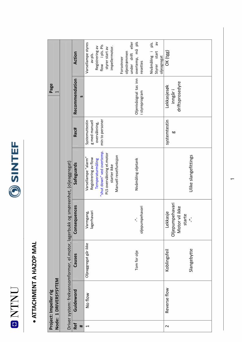
1
• ATT
ACHM
ENT
A HA
ZOP
MAL
Pr
ojec
t: Im
pelle
r rig
N
ode:
1 D
RIVE
RSYS
YTEM
Pa
ge
1 Dr
iver
syst
em: f
rekv
enso
mfo
rmer
, el.m
otor
, lag
erbu
kk o
g sm
øree
nhet
, (ol
jeag
greg
at)
Ref #
Gui
dew
ord
Caus
es
Cons
eque
nces
Sa
fegu
ards
Re
c#
Reco
mm
enda
tion
s Ac
tion
1 N
o flo
w
Olje
aggr
egat
går
ikke
Tom
for o
lje
Varm
gang
, la
gerh
avar
i -”-
olje
pum
peha
vari
Vars
ella
mpe
”al
arm
” Re
gist
rerin
g av
flow
Te
mpe
ratu
rmål
ing
”shu
t dow
n” v
ed o
vert
emp.
PL
S ov
ervå
knin
g el
.mot
or
star
ter i
kke
Man
uell
rese
tfun
ksjo
n
Niv
åmål
ing
olje
tank
Syst
emut
test
ing
med
man
uell
over
våkn
ing,
m
in to
per
sone
r
O
ljeni
våsig
nal t
as in
n i s
tyre
prog
ram
Vars
ella
mpe
styr
es
av p
ls.
Regi
stre
ring
av
flow
i pl
s. P
ls st
yrer
star
t av
impe
llerm
otor
.
Fors
vinn
er
olje
strø
mm
en
unde
r dr
ift
elle
r ov
erte
mp,
m
å pl
s re
sett
es
N
ivåm
ålin
g i
pls.
St
yrer
st
art
av
olje
agre
gat
2 Re
vers
e flo
w
Kobl
ings
feil
Sl
ange
bytt
e
Lekk
asje
O
ljepu
mpe
hava
ri M
otor
vil
ikke
st
arte
-”
-
U
like
slang
efitt
ings
syst
emte
stin
g Le
kkas
jesø
k in
ngår
i dr
iftsp
rose
dyre
OK
(tgg
)
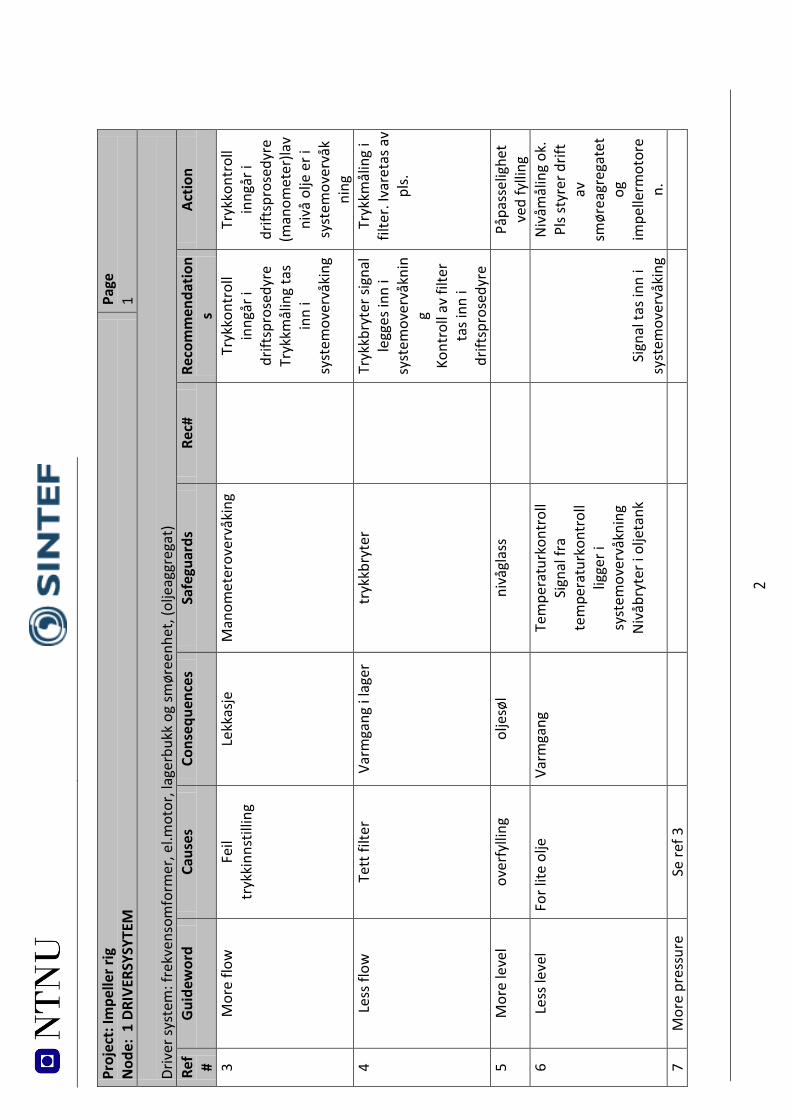
2 Pr
ojec
t: Im
pelle
r rig
N
ode:
1 D
RIVE
RSYS
YTEM
Pa
ge
1 Dr
iver
syst
em: f
rekv
enso
mfo
rmer
, el.m
otor
, lag
erbu
kk o
g sm
øree
nhet
, (ol
jeag
greg
at)
Ref #
Gui
dew
ord
Caus
es
Cons
eque
nces
Sa
fegu
ards
Re
c#
Reco
mm
enda
tion
s Ac
tion
3 M
ore
flow
Feil
tryk
kinn
still
ing
Lekk
asje
Man
omet
erov
ervå
king
Tryk
kont
roll
inng
år i
drift
spro
sedy
re
Tryk
kmål
ing
tas
inn
i sy
stem
over
våki
ng
Tryk
kont
roll
inng
år i
drift
spro
sedy
re
(man
omet
er)la
v ni
vå o
lje e
r i
syst
emov
ervå
kni
ng
4 Le
ss fl
ow
Tett
filte
r Va
rmga
ng i
lage
r tr
ykkb
ryte
r
Tryk
kbry
ter s
igna
l le
gges
inn
i sy
stem
over
våkn
ing
Kont
roll
av fi
lter
tas i
nn i
drift
spro
sedy
re
Tryk
kmål
ing
i fil
ter.
Ivar
etas
av
pls.
5 M
ore
leve
l
over
fylli
ng
olje
søl
nivå
glas
s
På
pass
elig
het
ved
fylli
ng
6 Le
ss le
vel
For l
ite o
lje
Varm
gang
Te
mpe
ratu
rkon
trol
l Si
gnal
fra
tem
pera
turk
ontr
oll
ligge
r i
syst
emov
ervå
knin
g N
ivåb
ryte
r i o
ljeta
nk
Sign
al ta
s inn
i sy
stem
over
våki
ng
Niv
åmål
ing
ok.
Pls s
tyre
r drif
t av
sm
ørea
greg
atet
og
im
pelle
rmot
ore
n.
7 M
ore
pres
sure
Se
ref 3
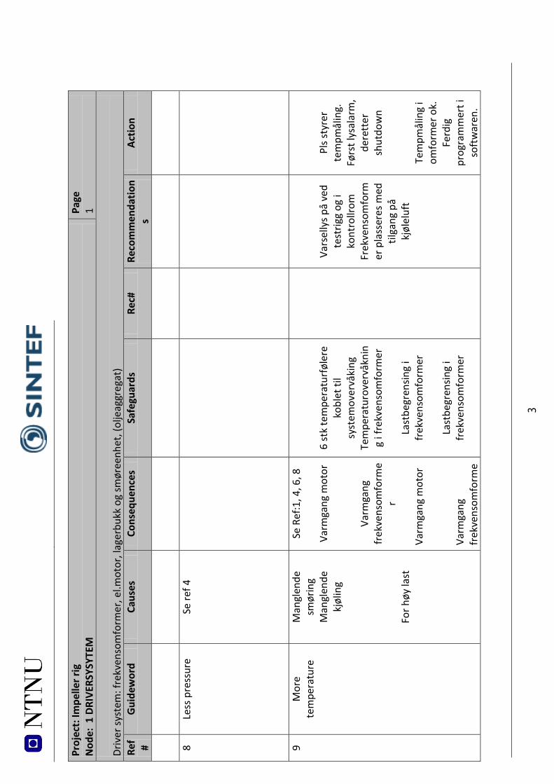
3 Pr
ojec
t: Im
pelle
r rig
N
ode:
1 D
RIVE
RSYS
YTEM
Pa
ge
1 Dr
iver
syst
em: f
rekv
enso
mfo
rmer
, el.m
otor
, lag
erbu
kk o
g sm
øree
nhet
, (ol
jeag
greg
at)
Ref #
Gui
dew
ord
Caus
es
Cons
eque
nces
Sa
fegu
ards
Re
c#
Reco
mm
enda
tion
s Ac
tion
8
Less
pre
ssur
e
Se re
f 4
9 M
ore
tem
pera
ture
Man
glen
de
smør
ing
Man
glen
de
kjøl
ing
Fo
r høy
last
Se R
ef:1
, 4, 6
, 8
Va
rmga
ng m
otor
Varm
gang
fr
ekve
nsom
form
er
Varm
gang
mot
or
Varm
gang
fr
ekve
nsom
form
e
6
stk
tem
pera
turf
øler
e ko
blet
til
syst
emov
ervå
king
Te
mpe
ratu
rove
rvåk
nin
g i f
rekv
enso
mfo
rmer
Last
begr
ensin
g i
frek
vens
omfo
rmer
Last
begr
ensin
g i
frek
vens
omfo
rmer
Vars
elly
s på
ved
test
rigg
og i
kont
rollr
om
Frek
vens
omfo
rmer
pla
sser
es m
ed
tilga
ng p
å kj
ølel
uft
Pl
s sty
rer
tem
pmål
ing.
Fø
rst l
ysal
arm
, de
rett
er
shut
dow
n
Tem
pmål
ing
i om
form
er o
k.
Ferd
ig
prog
ram
mer
t i
soft
war
en.
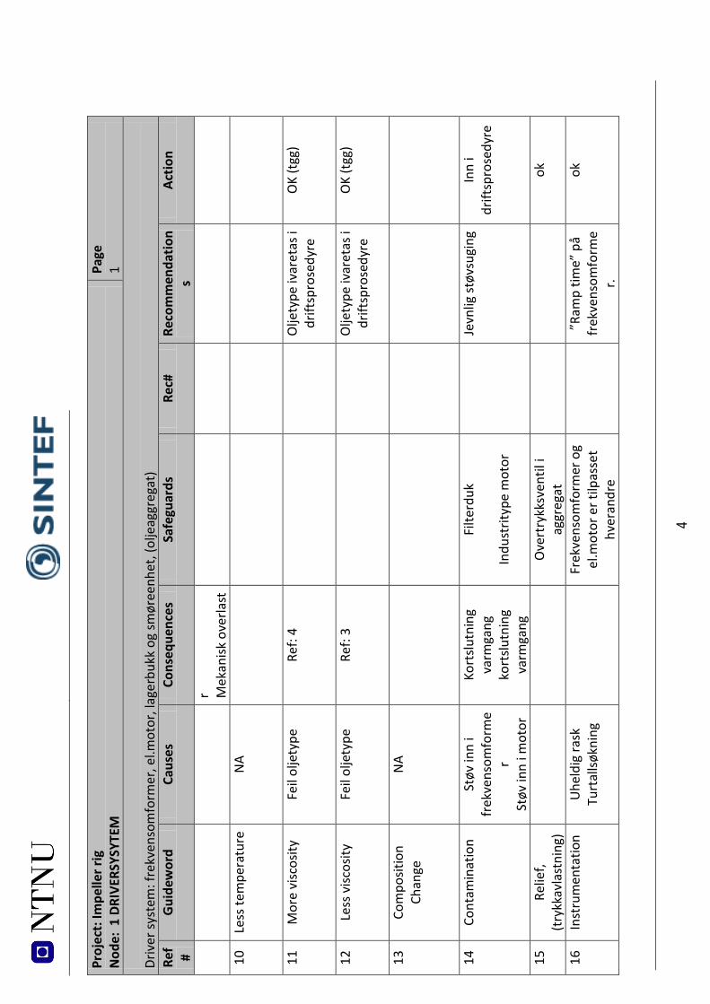
4 Pr
ojec
t: Im
pelle
r rig
N
ode:
1 D
RIVE
RSYS
YTEM
Pa
ge
1 Dr
iver
syst
em: f
rekv
enso
mfo
rmer
, el.m
otor
, lag
erbu
kk o
g sm
øree
nhet
, (ol
jeag
greg
at)
Ref #
Gui
dew
ord
Caus
es
Cons
eque
nces
Sa
fegu
ards
Re
c#
Reco
mm
enda
tion
s Ac
tion
r Mek
anisk
ove
rlast
10
Le
ss te
mpe
ratu
re
NA
11
Mor
e vi
scos
ity
Feil
olje
type
Re
f: 4
Olje
type
ivar
etas
i dr
iftsp
rose
dyre
O
K (t
gg)
12
Less
visc
osity
Feil
olje
type
Re
f: 3
Olje
type
ivar
etas
i dr
iftsp
rose
dyre
O
K (t
gg)
13
Com
posit
ion
Chan
ge
NA
14
Cont
amin
atio
n
Støv
inn
i fr
ekve
nsom
form
er
Støv
inn
i mot
or
Kort
slutn
ing
varm
gang
ko
rtslu
tnin
g va
rmga
ng
Filte
rduk
Indu
strit
ype
mot
or
Je
vnlig
støv
sugi
ng
Inn
i dr
iftsp
rose
dyre
15
Relie
f, (t
rykk
avla
stni
ng)
Ove
rtry
kksv
entil
i ag
greg
at
ok
16
Inst
rum
enta
tion
Uhe
ldig
rask
Tu
rtal
lsøkn
ing
Fr
ekve
nsom
form
er o
g el
.mot
or e
r tilp
asse
t hv
eran
dre
”R
amp
time”
på
frek
vens
omfo
rme
r.
ok
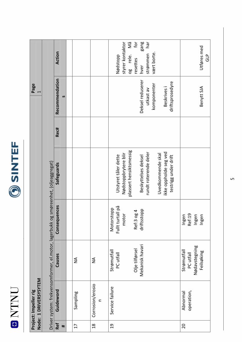
5 Pr
ojec
t: Im
pelle
r rig
N
ode:
1 D
RIVE
RSYS
YTEM
Pa
ge
1 Dr
iver
syst
em: f
rekv
enso
mfo
rmer
, el.m
otor
, lag
erbu
kk o
g sm
øree
nhet
, (ol
jeag
greg
at)
Ref #
Gui
dew
ord
Caus
es
Cons
eque
nces
Sa
fegu
ards
Re
c#
Reco
mm
enda
tion
s Ac
tion
17
Sa
mpl
ing
NA
18
Corr
osio
n/er
osio
n
NA
19
Serv
ice
failu
re
Strø
mut
fall
PC u
tfal
l
Olje
tilfø
rsel
M
ekan
isk h
avar
i
Mot
orst
opp
Fullt
turt
all p
å m
otor
Ref:3
og
4 dr
iftss
topp
U
tsty
ret t
åler
det
te
Nød
stop
pbry
tere
blir
pl
asse
rt h
ensik
tsm
essig
Besk
ytte
lses d
ekse
l ru
ndt r
oter
ende
del
er
U
vedk
omm
ende
skal
ik
ke o
ppho
lde
seg
ved
test
rigg
unde
r drif
t
Deks
el re
duse
rer
utka
st a
v ko
mpo
nent
er
Be
skriv
es i
drift
spro
sedy
re
N
ødst
opp
styr
er k
onta
ktor
og
re
le.
Må
rese
ttes
fo
r hv
er
gang
st
røm
men
ha
r væ
rt b
orte
.
20
Abno
rmal
op
erat
ion,
Strø
mut
fall
PC u
tfal
l N
ødav
steg
ning
Fe
ilsøk
ing
Inge
n Re
f:19
Inge
n In
gen
Be
nytt
SJA
U
tfør
es m
ed
GLP
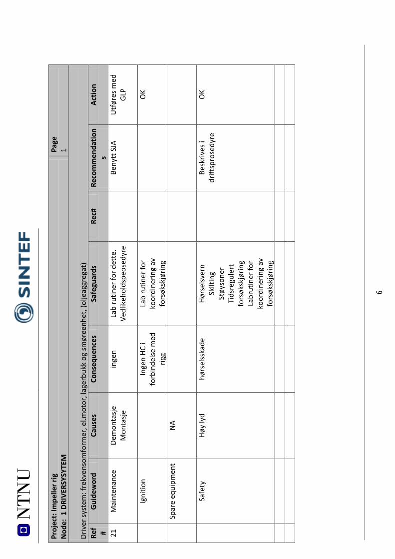
6 Pr
ojec
t: Im
pelle
r rig
N
ode:
1 D
RIVE
RSYS
YTEM
Pa
ge
1 Dr
iver
syst
em: f
rekv
enso
mfo
rmer
, el.m
otor
, lag
erbu
kk o
g sm
øree
nhet
, (ol
jeag
greg
at)
Ref #
Gui
dew
ord
Caus
es
Cons
eque
nces
Sa
fegu
ards
Re
c#
Reco
mm
enda
tion
s Ac
tion
21
Mai
nten
ance
Dem
onta
sje
Mon
tasje
in
gen
Lab
rutin
er fo
r det
te.
Vedl
ikeh
olds
peos
edyr
e
Beny
tt S
JA
Utf
øres
med
GL
P
Ig
nitio
n
In
gen
HC i
forb
inde
lse m
ed
rigg
Lab
rutin
er fo
r ko
ordi
nerin
g av
fo
rsøk
skjø
ring
OK
Sp
are
equi
pmen
t
NA
Sa
fety
Høy
lyd
hørs
elss
kade
Hø
rsel
sver
n Sk
iltin
g St
øyso
ner
Tids
regu
lert
fo
rsøk
skjø
ring
La
brut
iner
for
koor
dine
ring
av
fors
øksk
jørin
g
Be
skriv
es i
drift
spro
sedy
re
OK
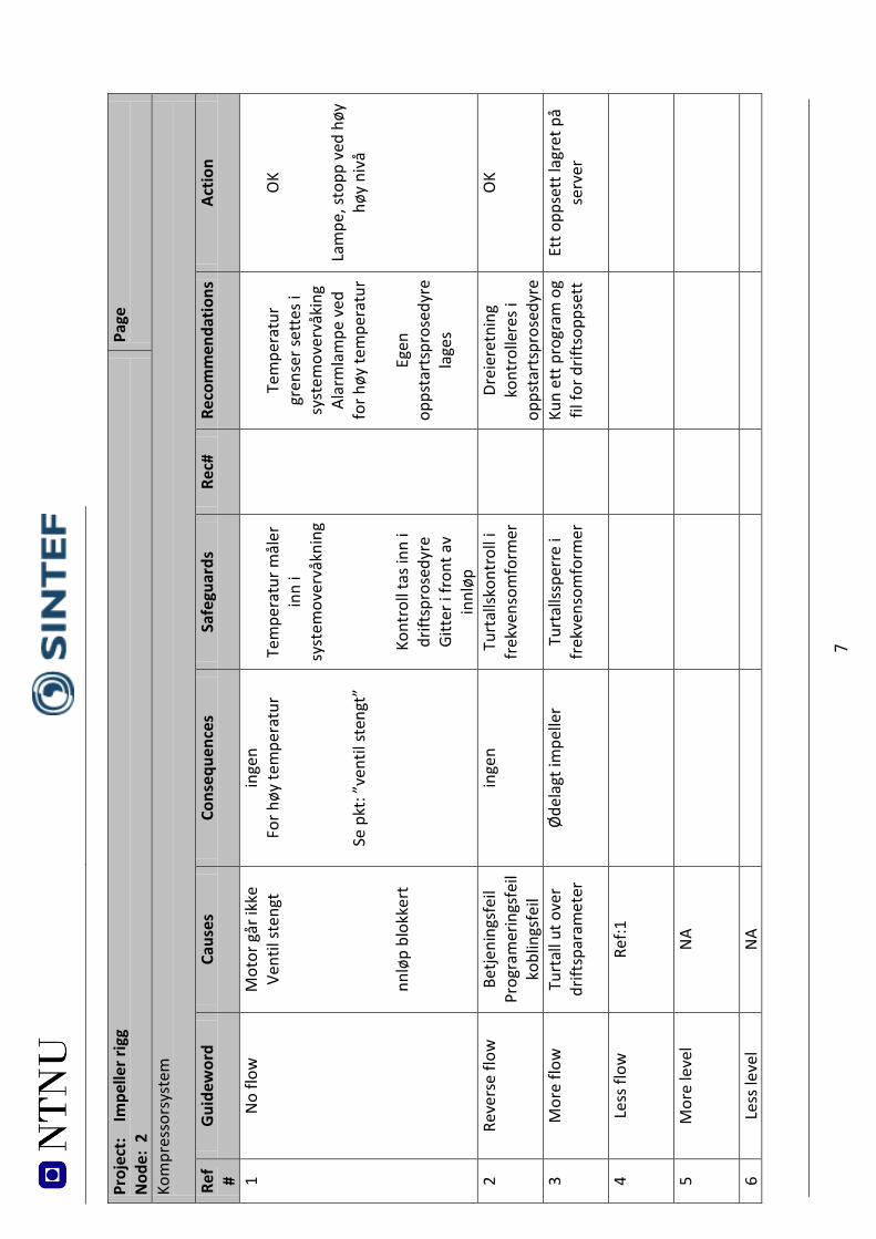
7 Pr
ojec
t:
Impe
ller r
igg
N
ode:
2
Page
Kom
pres
sors
yste
m
Ref #
Gui
dew
ord
Caus
es
Cons
eque
nces
Sa
fegu
ards
Re
c#
Reco
mm
enda
tions
Ac
tion
1 N
o flo
w
Mot
or g
år ik
ke
Vent
il st
engt
nnlø
p bl
okke
rt
inge
n Fo
r høy
tem
pera
tur
Se
pkt
: ”ve
ntil
sten
gt”
Te
mpe
ratu
r mål
er
inn
i sy
stem
over
våkn
ing
Ko
ntro
ll ta
s inn
i dr
iftsp
rose
dyre
Gi
tter
i fr
ont a
v in
nløp
Tem
pera
tur
gren
ser s
ette
s i
syst
emov
ervå
king
Al
arm
lam
pe v
ed
for h
øy te
mpe
ratu
r
Egen
op
psta
rtsp
rose
dyre
la
ges
OK
Lam
pe, s
topp
ved
høy
hø
y ni
vå
2 Re
vers
e flo
w
Betje
ning
sfei
l Pr
ogra
mer
ings
feil
kobl
ings
feil
inge
n Tu
rtal
lskon
trol
l i
frek
vens
omfo
rmer
Drei
eret
ning
ko
ntro
llere
s i
opps
tart
spro
sedy
re
OK
3 M
ore
flow
Turt
all u
t ove
r dr
iftsp
aram
eter
Ø
dela
gt im
pelle
r Tu
rtal
lsspe
rre
i fr
ekve
nsom
form
er
Ku
n et
t pro
gram
og
fil fo
r drif
tsop
pset
t Et
t opp
sett
lagr
et p
å se
rver
4 Le
ss fl
ow
Ref:1
5 M
ore
leve
l
NA
6 Le
ss le
vel
NA
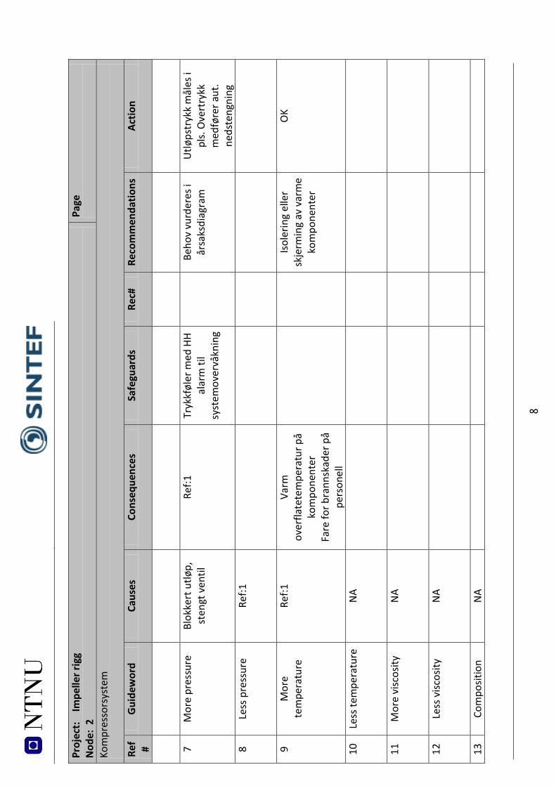
8 Pr
ojec
t:
Impe
ller r
igg
N
ode:
2
Page
Kom
pres
sors
yste
m
Ref #
Gui
dew
ord
Caus
es
Cons
eque
nces
Sa
fegu
ards
Re
c#
Reco
mm
enda
tions
Ac
tion
7
Mor
e pr
essu
re
Blok
kert
utlø
p,
sten
gt v
entil
Re
f:1
Tryk
kføl
er m
ed H
H al
arm
til
syst
emov
ervå
knin
g
Be
hov
vurd
eres
i år
saks
diag
ram
U
tløps
tryk
k m
åles
i pl
s. O
vert
rykk
m
edfø
rer a
ut.
neds
teng
ning
8
Less
pre
ssur
e
Ref:1
9 M
ore
tem
pera
ture
Ref:1
Va
rm
over
flate
tem
pera
tur p
å ko
mpo
nent
er
Fare
for b
rann
skad
er p
å pe
rson
ell
Isol
erin
g el
ler
skje
rmin
g av
var
me
kom
pone
nter
OK
10
Less
tem
pera
ture
NA
11
Mor
e vi
scos
ity
NA
12
Less
visc
osity
NA
13
Com
posit
ion
NA
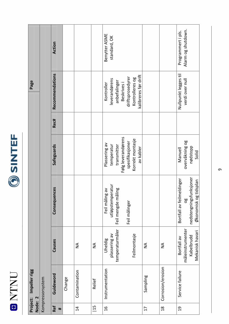
9 Pr
ojec
t:
Impe
ller r
igg
N
ode:
2
Page
Kom
pres
sors
yste
m
Ref #
Gui
dew
ord
Caus
es
Cons
eque
nces
Sa
fegu
ards
Re
c#
Reco
mm
enda
tions
Ac
tion
Chan
ge
14
Co
ntam
inat
ion
NA
|15
Relie
f
NA
16
Inst
rum
enta
tion
Uhe
ldig
pl
asse
ring
av
tem
pera
turm
åler
Feilm
onta
sje
Feil
mål
ing
av
utlø
pste
mpe
ratu
r Fe
il m
engd
e m
ålin
g
Feil
mål
inge
r
Plas
serin
g av
te
mpe
ratu
r tr
ansm
itter
Fø
lg le
vera
ndør
ens
spes
ifika
sjone
r Ko
rrek
t mon
tasje
av
kab
ler
Ko
ntro
ller
leve
rand
øren
s an
befa
linge
r Be
skriv
es i
drift
spro
sedy
rer
Kont
rolle
res o
g ka
libre
res f
ør d
rift
Beny
tter
ASM
E st
anda
rd, O
K
17
Sam
plin
g
NA
18
Corr
osio
n/er
osio
n
NA
19
Serv
ice
failu
re
Bort
fall
av
mål
eins
trum
ente
r Ka
belb
rudd
M
ekan
isk h
avar
i
Bort
fall
av fe
ilmel
ding
er
og
neds
teng
ning
sfun
ksjo
ner
Øko
nom
isk o
g tid
spla
n
Man
uell
over
våkn
ing
og
nøds
topp
So
lid
N
ullp
unkt
legg
es ti
l ve
rdi o
ver n
ull
Prog
ram
mer
t i p
ls.
Alar
m o
g sh
utdo
wn.
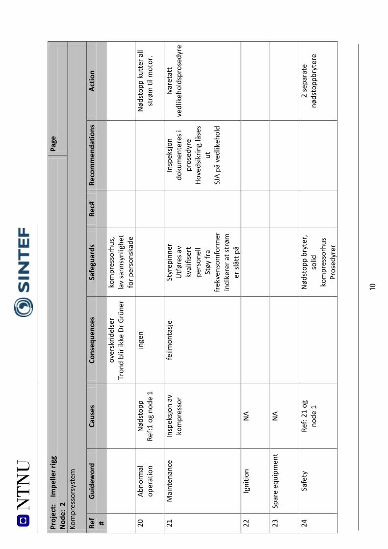
10
Proj
ect:
Im
pelle
r rig
g
Nod
e: 2
Pa
ge
Ko
mpr
esso
rsys
tem
Re
f # G
uide
wor
d Ca
uses
Co
nseq
uenc
es
Safe
guar
ds
Rec#
Re
com
men
datio
ns
Actio
n
over
skrid
else
r Tr
ond
blir
ikke
Dr G
rüne
r ko
mpr
esso
rhus
, la
v sa
nnsy
nlig
het
for p
erso
nska
de
20
Abno
rmal
op
erat
ion
Nød
stop
p Re
f:1 o
g no
de 1
in
gen
N
ødst
opp
kutt
er a
ll st
røm
til m
otor
.
21
Mai
nten
ance
Insp
eksjo
n av
ko
mpr
esso
r fe
ilmon
tasje
St
yrep
inne
r U
tfør
es a
v kv
alifi
sert
pe
rson
ell
Støy
fra
frek
vens
omfo
rmer
in
dike
rer a
t str
øm
er sl
ått p
å
In
spek
sjon
doku
men
tere
s i
pros
edyr
e Ho
veds
ikrin
g lå
ses
ut
SJA
på v
edlik
ehol
d
Ivar
etat
t ve
dlik
ehol
dspr
osed
yre
22
Igni
tion
NA
23
Spar
e eq
uipm
ent
NA
24
Safe
ty
Ref:
21 o
g
node
1
N
ødst
opp
bryt
er,
solid
ko
mpr
esso
rhus
Pr
osed
yrer
2 se
para
te
nøds
topp
bryt
ere
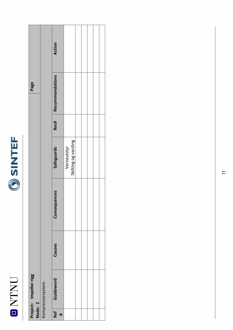
11
Proj
ect:
Im
pelle
r rig
g
Nod
e: 2
Pa
ge
Ko
mpr
esso
rsys
tem
Re
f # G
uide
wor
d Ca
uses
Co
nseq
uenc
es
Safe
guar
ds
Rec#
Re
com
men
datio
ns
Actio
n
Vern
euts
tyr
Skilt
ing
og v
arsli
ng

1
• ATTACHMENT B PRØVESERTIFIKAT FOR LOKAL TRYKKTESTING Trykktesten skal utføres I følge NS-EN 13445 del 5 (Inspeksjon og prøving). Se også prosedyre for trykktesting gjeldende for VATL lab Trykkpåkjent utstyr: ………………………. Benyttes i rigg: …………………………………………. Design trykk for utstyr: …………………..bara Maksimum tillatt trykk: …………………..bara (i.e. burst pressure om kjent) Maksimum driftstrykk i denne rigg: …………………..bara Prøvetrykket skal fastlegges i følge standarden og med hensyn til maksimum tillatt trykk. Prøvetrykk: ……………..bara (………. x maksimum driftstrykk) I følge standard Test medium: Temperatur: °C Start: Tid:
Trykk: bara Slutt: Tid: Trykk: bara Eventuelle repetisjoner fra atm. trykk til maksimum prøvetrykk:…………….
Test trykket, dato for testing og maksimum tillatt driftstrykk skal markers på (skilt eller innslått) Sted og dato Signatur
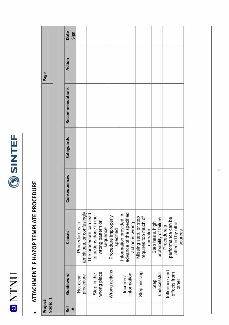
1 •
ATTA
CHM
ENT
F H
AZO
P TE
MPL
ATE
PRO
CEDU
RE
Proj
ect:
Nod
e: 1
Pa
ge
Re
f # G
uide
wor
d Ca
uses
Co
nseq
uenc
es
Safe
guar
ds
Reco
mm
enda
tions
Ac
tion
Date
Si
gn
N
ot c
lear
pr
oced
ure
Pro
cedu
re is
to
ambi
tious
, or c
onfu
sing
ly
S
tep
in th
e w
rong
pla
ce
The
proc
edur
e ca
n le
ad
to a
ctio
ns d
one
in th
e w
rong
pat
tern
or
sequ
ence
W
rong
act
ions
Pro
cedu
re im
prop
erly
sp
ecifi
ed
In
corre
ct
info
rmat
ion
Info
rmat
ion
prov
ided
in
adva
nce
of th
e sp
ecifi
ed
actio
n is
wro
ng
S
tep
mis
sing
Mis
sing
ste
p, o
r ste
p re
quire
s to
o m
uch
of
oper
ator
S
tep
unsu
cess
ful
Ste
p ha
s a
high
pr
obab
ility
of fa
ilure
In
fluen
ce a
nd
effe
cts
from
ot
her
Pro
cedu
re's
pe
rform
ance
can
be
affe
cted
by
othe
r so
urce
s
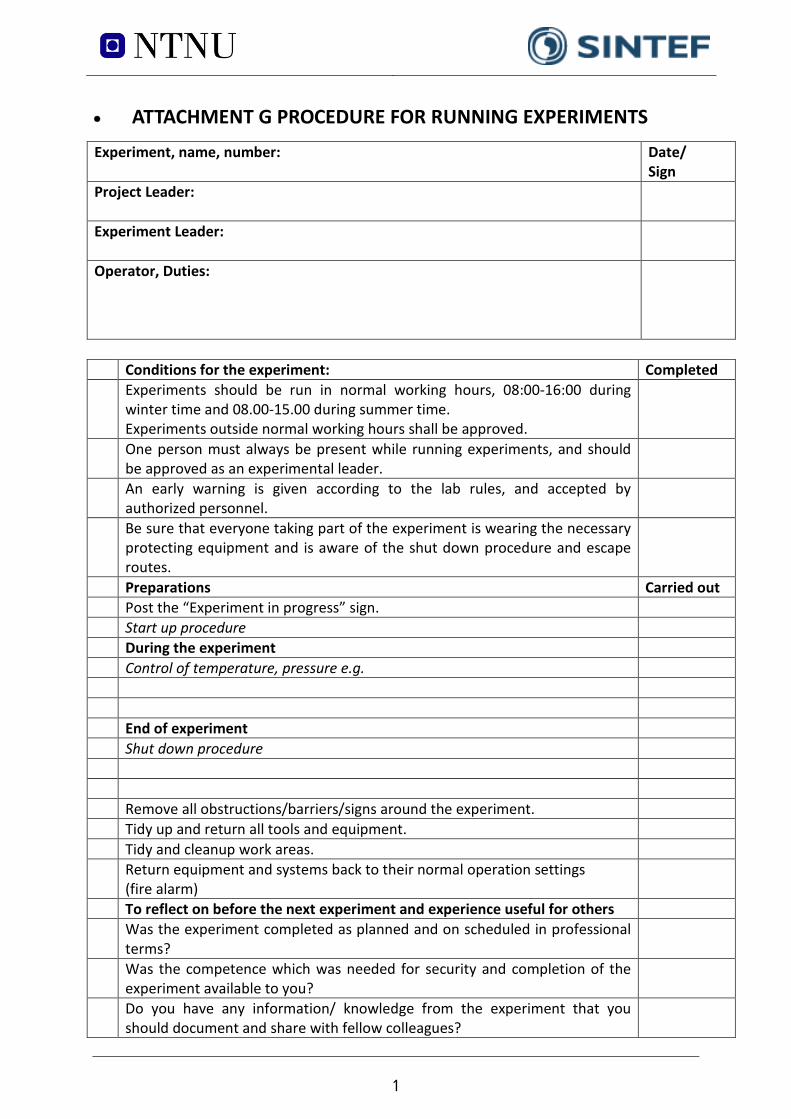
1
• ATTACHMENT G PROCEDURE FOR RUNNING EXPERIMENTS
Experiment, name, number:
Date/ Sign
Project Leader:
Experiment Leader:
Operator, Duties:
Conditions for the experiment: Completed Experiments should be run in normal working hours, 08:00-16:00 during
winter time and 08.00-15.00 during summer time. Experiments outside normal working hours shall be approved.
One person must always be present while running experiments, and should be approved as an experimental leader.
An early warning is given according to the lab rules, and accepted by authorized personnel.
Be sure that everyone taking part of the experiment is wearing the necessary protecting equipment and is aware of the shut down procedure and escape routes.
Preparations Carried out Post the “Experiment in progress” sign. Start up procedure During the experiment Control of temperature, pressure e.g. End of experiment Shut down procedure Remove all obstructions/barriers/signs around the experiment. Tidy up and return all tools and equipment. Tidy and cleanup work areas. Return equipment and systems back to their normal operation settings
(fire alarm)
To reflect on before the next experiment and experience useful for others Was the experiment completed as planned and on scheduled in professional
terms?
Was the competence which was needed for security and completion of the experiment available to you?
Do you have any information/ knowledge from the experiment that you should document and share with fellow colleagues?

2
• ATTACHMENT H TRAINING OF OPERATORS
Experiment, name, number:
Date/ Sign
Project Leader:
Experiment Leader:
Operator
Knowledge to EPT LAB in general Lab
- Access -routines and roules -working hour
Knowledge about the evacuation procedures. Activity calendar for the Lab Knowledge to the experiments Procedures for the experiments Emergency shutdown. Nearest fire and first aid station.
Operatør HMS responsible Dato Dato
Signert
Signert

3
14 ATTACHMENT I FORM FOR SAFE JOB ANALYSIS
SJA tittel: Dato: Sted: Kryss av for utfylt sjekkliste: Deltakere:
SJA-ansvarlig: Arbeidsbeskrivelse: (Hva og hvordan?)
Risiko forbundet med arbeidet:
Beskyttelse/sikring: (tiltaksplan, se neste side)
Konklusjon/kommentar:
Anbefaling/godkjenning: Dato/Signatur: Anbefaling/godkjenning: Dato/Signatur:
SJA-ansvarlig: Områdeansvarlig:
Ansvarlig for utføring: Annen (stilling):
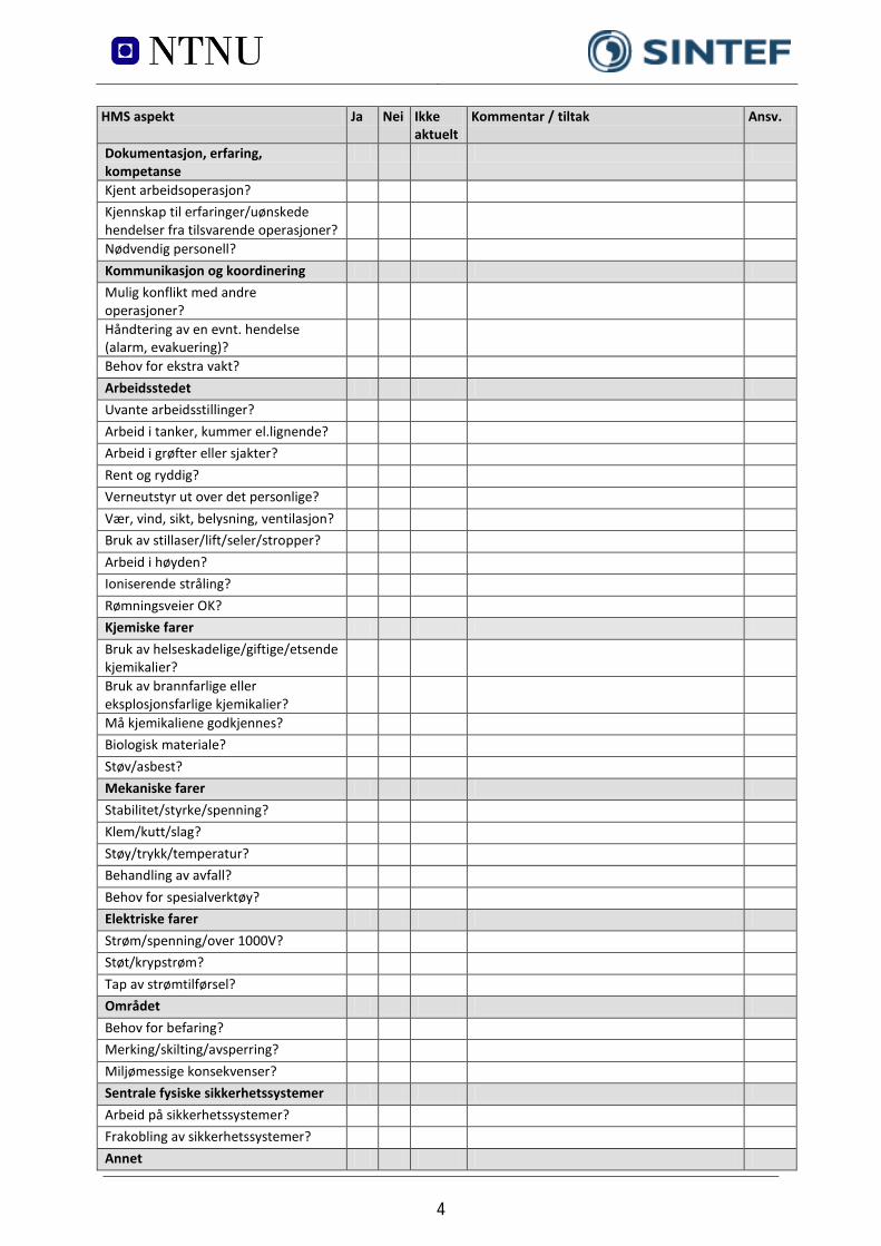
4
HMS aspekt Ja Nei Ikke aktuelt
Kommentar / tiltak Ansv.
Dokumentasjon, erfaring, kompetanse
Kjent arbeidsoperasjon? Kjennskap til erfaringer/uønskede hendelser fra tilsvarende operasjoner?
Nødvendig personell? Kommunikasjon og koordinering Mulig konflikt med andre operasjoner?
Håndtering av en evnt. hendelse (alarm, evakuering)?
Behov for ekstra vakt? Arbeidsstedet Uvante arbeidsstillinger? Arbeid i tanker, kummer el.lignende? Arbeid i grøfter eller sjakter? Rent og ryddig? Verneutstyr ut over det personlige? Vær, vind, sikt, belysning, ventilasjon? Bruk av stillaser/lift/seler/stropper? Arbeid i høyden? Ioniserende stråling? Rømningsveier OK? Kjemiske farer Bruk av helseskadelige/giftige/etsende kjemikalier?
Bruk av brannfarlige eller eksplosjonsfarlige kjemikalier?
Må kjemikaliene godkjennes? Biologisk materiale? Støv/asbest? Mekaniske farer Stabilitet/styrke/spenning? Klem/kutt/slag? Støy/trykk/temperatur? Behandling av avfall? Behov for spesialverktøy? Elektriske farer Strøm/spenning/over 1000V? Støt/krypstrøm? Tap av strømtilførsel? Området Behov for befaring? Merking/skilting/avsperring? Miljømessige konsekvenser? Sentrale fysiske sikkerhetssystemer Arbeid på sikkerhetssystemer? Frakobling av sikkerhetssystemer? Annet

5
15 ATTACHMENT J APPARATURKORT UNITCARD
Apparatur/unit
Dette kortet SKAL henges godt synlig på apparaturen!This card MUST be posted on a visible place on the unit! Faglig Ansvarlig (Scientific Responsible)
Telefon mobil/privat (Phone no. mobile/private)
Apparaturansvarlig (Unit Responsible)
Telefon mobil/privat (Phone no. mobile/private)
Sikkerhetsrisikoer (Safety hazards) Sikkerhetsregler Safety rules) Nødstopp prosedyre Emergency shutdown)
Her finner du (Here you will find):
Prosedyrer (Procedures) Bruksanvisning (Users manual)
Nærmeste (nearest)
Brannslukningsapparat (fire extinguisher) Førstehjelpsskap (first aid cabinet) NTNU Institutt for energi og prosessteknikk
SINTEF Energi Avdeling energiprosesser
Dato
Dato
Signert
Signert

6
16 ATTACHMENT K FORSØK PÅGÅR KORT
Forsøk pågår! Experiment in progress!
Dette kort skal settes opp før forsøk kan påbegynnes This card has to be posted before an experiment can start Ansvarlig / Responsible
Telefon jobb/mobil/hjemme
Operatører/Operators
Forsøksperiode/Experiment time(start – slutt)
Prosjektleder
Prosjekt
Kort beskrivelse av forsøket og relaterte farer Short description of the experiment and related hazards
NTNU Institutt for energi og prosessteknikk
SINTEF Energi Avdeling energiprosesser
Dato
Dato
Signert
Signert
1. Grüner, T.G.a.L.E.B., Aerodynamic instability investigation of a centrifugal compressor
exposed to wet gas. 2010.

7

8
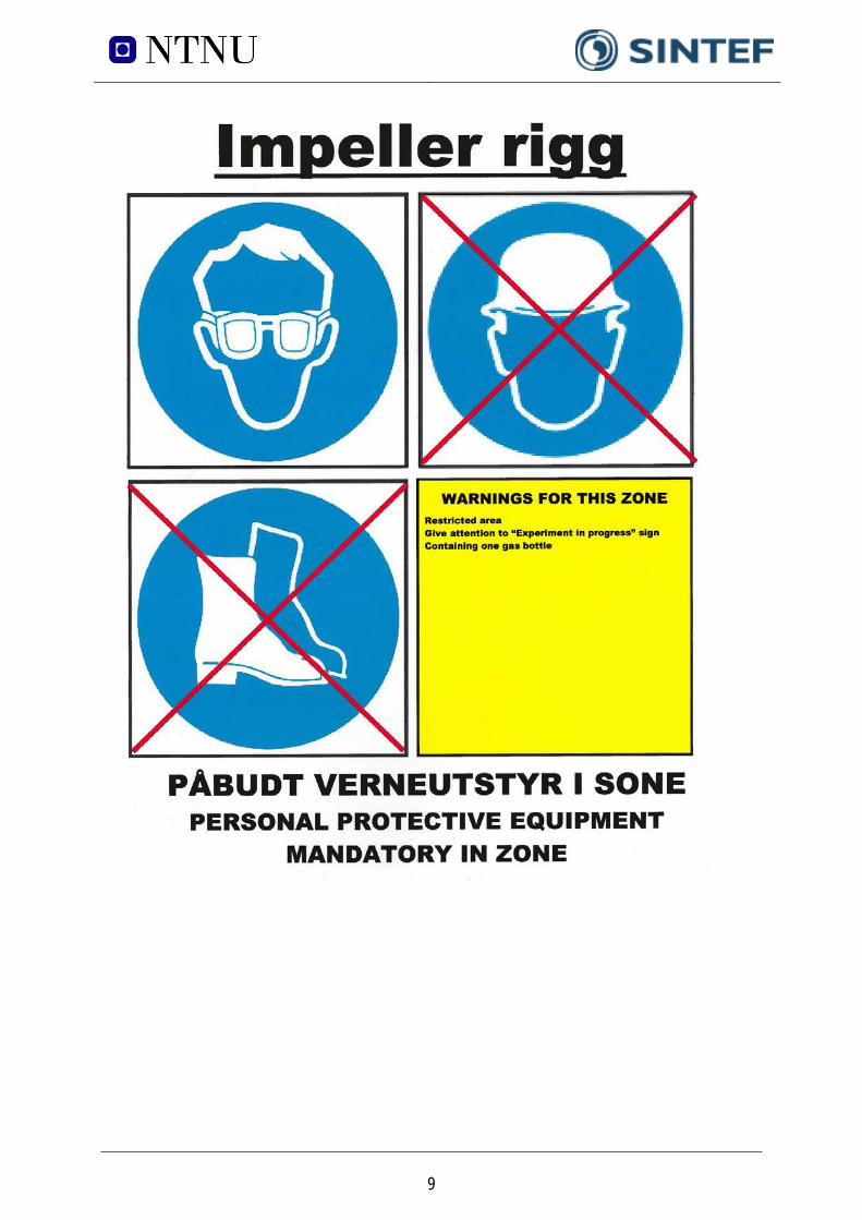
9
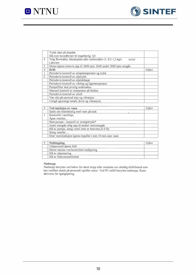
10

Appendix E: Gantt chart
Appendix E: Gantt chart
Appendix E provides an overview of the planned activities during the master thesis.
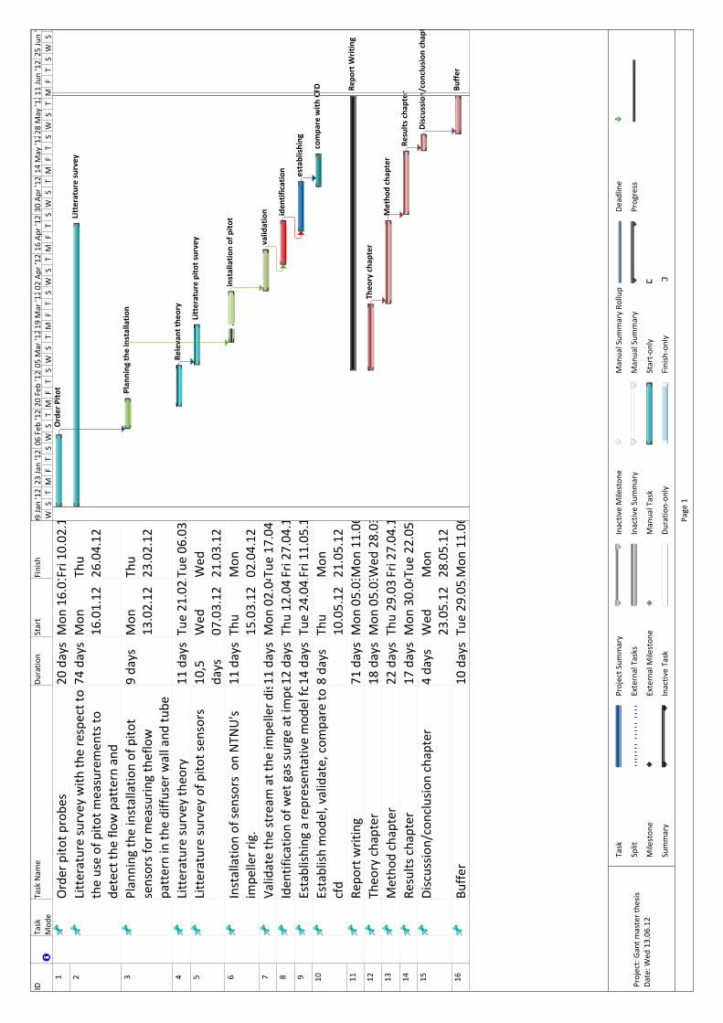
IDTask
Mod
eTask Nam
eDu
ratio
nStart
Finish
1Order pito
t probe
s20
daysMon
16.01Fri 10.02.1
2Litterature survey with
the respect to
the use of pito
t measuremen
ts to
de
tect th
e flo
w pattern and
74 daysMon
16.01.12
Thu
26.04.12
3Planning
the installatio
n of pito
t sensors for m
easurin
g theflow
pattern in th
e diffu
ser w
all and
tube
9 days
Mon
13.02.12
Thu
23.02.12
4Litterature survey th
eory
11 daysTue 21.02.Tue 06.03.
5Litterature survey of p
itot sen
sors
10,5
days
Wed
07.03.12
Wed
21.03.12
6Installatio
n of se
nsors on
NTN
U's
impe
ller rig.
11 daysThu
15.03.12
Mon
02.04.12
7Va
lidate the stream
at the
impe
ller d
is11 days
Mon
02.04Tue 17.04.
8Iden
tification of wet gas su
rge at im
pe12
daysThu 12.04Fri 27.04.1
9Establish
ing a represen
tativ
e mod
el fo
14 daysTue 24.04.Fri 11.05.1
10Establish
mod
el, validate, com
pare to
cfd
8 days
Thu
10.05.12
Mon
21.05.12
11Re
port writing
71 daysMon
05.03Mon
11.06
12Theo
ry chapter
18 daysMon
05.03Wed
28.03
13Metho
d chapter
22 daysThu 29.03Fri 27.04.1
14Re
sults chapter
17 daysMon
30.04Tue 22.05.
15Discussio
n/conclusio
n chapter
4 days
Wed
23.05.12
Mon
28.05.12
16Bu
ffer
10 daysTue 29.05.Mon
11.06
Order Pito
t
Litterature survey
Plan
ning
the installatio
n
Relevant th
eory
Litterature pitot survey
installatio
n of pito
t
valid
ation iden
tification establishing
compa
re with
CFD Re
port W
riting
Theo
ry cha
pter
Metho
d chap
ter
Results
cha
pter
Discussion/conclusion
cha
pt
Buffer
WS
TM
FT
SW
ST
MF
TS
WS
TM
FT
SW
ST
MF
TS
WS
TM
FT
SW
ST
MF
TS
WS
09 Ja
n '1223
Jan '1206
Feb
'1220
Feb
'1205
Mar '1219
Mar '1202
Apr '1216
Apr '1230
Apr '1214
May '122
8 May '121
1 Jun '1225
Jun '
Task
Split
Mileston
e
Summary
Project S
ummary
External Tasks
External M
ileston
e
Inactiv
e Task
Inactiv
e Mileston
e
Inactiv
e Summary
Manual Task
Duratio
n‐on
ly
Manual Sum
mary Ro
llup
Manual Sum
mary
Start‐on
ly
Finish‐only
Deadline
Progress
Page 1
Project: Gant m
aster the
sisDa
te: W
ed 13.06
.12